Embed Size (px)
Citation preview
Robust nonlinear control design for amissile using backstepping
Examensarbete utfort i Reglerteknikvid Tekniska Hogskolan i Linkoping
av
Johan Dahlgren
Reg nr: LiTH-ISY-EX-3300-2002

Robust nonlinear control design for amissile using backstepping
Examensarbete utfort i Reglerteknikvid Tekniska Hogskolan i Linkoping
av
Johan Dahlgren
Reg nr: LiTH-ISY-EX-3300-2002
Supervisor: Ola HarkegardHenrik Jonson
Examiner: Torkel Glad
Linkoping, 27th January 2003.

Avdelning, Institution Division, Department
Institutionen för Systemteknik 581 83 LINKÖPING
Datum Date 2002-12-19
Språk Language
Rapporttyp Report category
ISBN
Svenska/Swedish X Engelska/English
Licentiatavhandling X Examensarbete
ISRN LITH-ISY-EX-3300-2002
C-uppsats D-uppsats
Serietitel och serienummer Title of series, numbering
ISSN
Övrig rapport ____
URL för elektronisk version http://www.ep.liu.se/exjobb/isy/2002/3300/
Titel Title
Robust olinjär missilstyrning med hjälp av backstepping Robust nonlinear control design for a missile using backstepping
Författare Author
Johan Dahlgren
Sammanfattning Abstract This thesis has been performed at SAAB Bofors Dynamics. The purpose was to derive a robust control design for a nonlinear missile using backstepping. A particularly interesting matter was to see how different design choices affect the robustness. Backstepping is a relatively new design method for nonlinear systems which leads to globally stabilizing control laws. By making wise decisions in the design the resulting closed loop can receive significant robustness. The method also makes it possible to benefit from naturally stabilizing aerodynamic forces and momentums. It is based on Lyapunov theory and the control laws and a Lyapunov function are derived simultaneously. This Lyapunov function is used to guarantee stability. In this thesis the control laws for the missile are first derived by using backstepping. The missile dynamics are described with aerodynamic coeffcients with corresponding uncertainties. The robustness of the design w.r.t. the aerodynamic uncertainties is then studied further in detail. One way to analyze how the stability is affected by the errors in the coeffcients is presented. To improve the robustness and remove static errors, dynamics are introduced in the control laws by adding an integrator. One conclusion that has been reached is that it is hard to immediately determine how a certain design choice affects the robustness. Instead it is at the point when algebraic expressions for the closed loop system have been obtained, that it is possible to analyze the affects of a certain design choice. The designed control laws are evaluated by simulations which shows satisfactory results.
Nyckelord Keyword backstepping, nonlinear, robust, missile, integral action

Abstract
This thesis has been performed at SAAB Bofors Dynamics. The purpose wasto derive a robust control design for a nonlinear missile using backstepping. Aparticularly interesting matter was to see how different design choices affect therobustness. Backstepping is a relatively new design method for nonlinear systemswhich leads to globally stabilizing control laws. By making wise decisions in thedesign the resulting closed loop can receive significant robustness. The methodalso makes it possible to benefit from naturally stabilizing aerodynamic forces andmomentums. It is based on Lyapunov theory and the control laws and a Lyapunovfunction are derived simultaneously. This Lyapunov function is used to guaranteestability. In this thesis the control laws for the missile are first derived by usingbackstepping. The missile dynamics are described with aerodynamic coefficientswith corresponding uncertainties. The robustness of the design w.r.t. the aerody-namic uncertainties is then studied further in detail. One way to analyze how thestability is affected by the errors in the coefficients is presented. To improve therobustness and remove static errors, dynamics are introduced in the control lawsby adding an integrator. One conclusion that has been reached is that it is hard toimmediately determine how a certain design choice affects the robustness. Insteadit is at the point when algebraic expressions for the closed loop system have beenobtained, that it is possible to analyze the affects of a certain design choice. Thedesigned control laws are evaluated by simulations which shows satisfactory results.
Keywords: backstepping, nonlinear, robust, missile, integral action
i

ii
Acknowledgment
First of all a would like to thank my two supervisors, Henrik Jonsson at SAABBofors Dynamics and Ola Harkegard at Linkopings University. The have given megood support and advises. I would also like to thank Professor Torkel Glad, myexaminer.
Besides these key persons i also would like to thank: all the people at floor 5at SAAB Bofors Dynamics in Linkoping for their kind reception. Rebecca, Lindaand Torbjorn Crona for proof-reading the report and providing valuable comments.
iii

iv
Notation
Symbols
x, X boldface letters are used for vectors, matrices and sets.R the set of real numbersu,U control inputx1 . . . xn state variablesV (x) Lyapunov functionxref
1 reference value of x1
xdes1 desired value of x1
a estimated value of the variable a that is used in the control laws
Operators and functions
||x|| Euclidian normV = dV
dt time derivative of V∇V (x, y) =
(∂V (x)
∂x , ∂V (x)∂y
)gradient of V (x, y)
Vx(x) =(
∂V (x)∂x1
, . . . , ∂V (x)∂xn
)gradient of V (x)
F ′(z1) = dF (z1)dz1
derivative of F w.r.t. its only argument z1
Abbreviations
clf Control Lyapunov Function
v
Missile nomenclature
State variables
Symbol Unit Definitionα rad,degrees angle of attackβ rad,degrees sideslip anglep rad/s roll rateq rad/s pitch rater rad/s yaw rateV = (u, v, w) body-axes velocityu m/s longitudinal velocityv m/s lateral velocityw m/s normal velocityaz
ms2 accleration in the normal direction
ayms2 acceleration in the lateral direction
Fin deflections
Symbol Unit Definitionδa rad,degrees aileron deflectionδe rad,degrees elevator deflectionδr rad/s rudder deflection
Missile data
Symbol Unit Definitionm kg massS m2 aerodynamic reference aread m diameter
I =
Ixx 0 00 Iyy 00 0 Izz
kgm2 inertial matrix
vi
Contents
1 Introduction 11.1 Background . . . . . . . . . . . . . . . . . . . . . . . . . . . . . . . . 11.2 Purpose . . . . . . . . . . . . . . . . . . . . . . . . . . . . . . . . . . 11.3 Method . . . . . . . . . . . . . . . . . . . . . . . . . . . . . . . . . . 11.4 Limitations . . . . . . . . . . . . . . . . . . . . . . . . . . . . . . . . 21.5 Outline of the thesis . . . . . . . . . . . . . . . . . . . . . . . . . . . 2
2 Basic theory 32.1 General non-linear theory . . . . . . . . . . . . . . . . . . . . . . . . 32.2 Lyapunov theory . . . . . . . . . . . . . . . . . . . . . . . . . . . . . 4
2.2.1 A geometrical interpretation of the direct method of Lyapunov 52.3 Lyapunov theory and control design . . . . . . . . . . . . . . . . . . 7
3 Backstepping 93.1 Backstepping design procedure . . . . . . . . . . . . . . . . . . . . . 93.2 Aspects on backstepping . . . . . . . . . . . . . . . . . . . . . . . . . 10
3.2.1 Design choices . . . . . . . . . . . . . . . . . . . . . . . . . . 103.2.2 Which system can be handled . . . . . . . . . . . . . . . . . . 11
4 The missile 134.1 Introduction to the missile . . . . . . . . . . . . . . . . . . . . . . . . 13
4.1.1 Guidance, Navigation and Control system (GN&C) . . . . . . 144.1.2 Definitions . . . . . . . . . . . . . . . . . . . . . . . . . . . . 154.1.3 Maneuvering . . . . . . . . . . . . . . . . . . . . . . . . . . . 164.1.4 Actuator dynamics . . . . . . . . . . . . . . . . . . . . . . . . 17
4.2 Deriving a model of the missile . . . . . . . . . . . . . . . . . . . . . 174.2.1 Basic rigid body dynamics . . . . . . . . . . . . . . . . . . . . 174.2.2 Assumptions . . . . . . . . . . . . . . . . . . . . . . . . . . . 184.2.3 Equations . . . . . . . . . . . . . . . . . . . . . . . . . . . . . 194.2.4 State-space representation . . . . . . . . . . . . . . . . . . . . 214.2.5 Comments about the aerodynamic coefficients . . . . . . . . . 214.2.6 The simulation model . . . . . . . . . . . . . . . . . . . . . . 22
vii
viii Contents
5 Backstepping design for the missile 235.1 Control objectives . . . . . . . . . . . . . . . . . . . . . . . . . . . . 23
5.1.1 Conversion of the accelerations . . . . . . . . . . . . . . . . . 235.2 Backstepping design . . . . . . . . . . . . . . . . . . . . . . . . . . . 25
5.2.1 Controlling the pitch-dynamics . . . . . . . . . . . . . . . . . 255.2.2 Controlling the yaw -dynamics . . . . . . . . . . . . . . . . . . 285.2.3 Controlling the roll-dynamics . . . . . . . . . . . . . . . . . . 305.2.4 Combining the control inputs . . . . . . . . . . . . . . . . . . 30
5.3 Aspects on the design . . . . . . . . . . . . . . . . . . . . . . . . . . 315.3.1 Cascaded control structure . . . . . . . . . . . . . . . . . . . 315.3.2 Tuning of the design parameters . . . . . . . . . . . . . . . . 315.3.3 Robustness of the design . . . . . . . . . . . . . . . . . . . . . 335.3.4 Exploring some design flexibilities . . . . . . . . . . . . . . . 35
5.4 Simulation . . . . . . . . . . . . . . . . . . . . . . . . . . . . . . . . . 375.4.1 Conditions . . . . . . . . . . . . . . . . . . . . . . . . . . . . 375.4.2 Controller parameters . . . . . . . . . . . . . . . . . . . . . . 375.4.3 Simulation results . . . . . . . . . . . . . . . . . . . . . . . . 37
5.5 Summary . . . . . . . . . . . . . . . . . . . . . . . . . . . . . . . . . 385.6 Simulation plots . . . . . . . . . . . . . . . . . . . . . . . . . . . . . 39
6 Dealing with uncertainties 416.1 Extended robustness discussion . . . . . . . . . . . . . . . . . . . . . 41
6.1.1 Problem review . . . . . . . . . . . . . . . . . . . . . . . . . . 416.1.2 Using level curves for stability analysis . . . . . . . . . . . . . 426.1.3 Identifying the ∆Ez2 -terms and ∆Ez1z2 -terms . . . . . . . . . 456.1.4 Simulations . . . . . . . . . . . . . . . . . . . . . . . . . . . . 46
6.2 Adding dynamics to the controller . . . . . . . . . . . . . . . . . . . 496.2.1 Introduction . . . . . . . . . . . . . . . . . . . . . . . . . . . 496.2.2 Theoretical background . . . . . . . . . . . . . . . . . . . . . 496.2.3 Adding the integrator to the previous design . . . . . . . . . 506.2.4 Simulation results . . . . . . . . . . . . . . . . . . . . . . . . 51
6.3 Increasing the gain in the backstepping loop . . . . . . . . . . . . . . 546.3.1 A level curve discussion . . . . . . . . . . . . . . . . . . . . . 55
6.4 Summary . . . . . . . . . . . . . . . . . . . . . . . . . . . . . . . . . 566.5 Simulation plots . . . . . . . . . . . . . . . . . . . . . . . . . . . . . 57
7 Conclusions and future work 637.1 Conclusions . . . . . . . . . . . . . . . . . . . . . . . . . . . . . . . . 637.2 Future work . . . . . . . . . . . . . . . . . . . . . . . . . . . . . . . . 63
A Missile data 67
B Aerodynamic coefficients 69
Chapter 1
Introduction
1.1 Background
Over the last two decades there has been a development in design methods forcontrol of nonlinear dynamic systems. Several new methods have been inventedand one of the more recent method is backstepping. At SAAB Bofors Dynamicsthere is an interest to follow how this development is proceeding.
1.2 Purpose
The main purpose of this thesis is to present a controller for a missile designed withbackstepping for SAAB. From the results reached in this report, SAAB can decidewhether backstepping is a design method of interest for their applications. Themissile dynamics are described with aerodynamic coefficients with correspondinguncertainties. Focus is therefore drawn to make the design robust against theseuncertainties in the aerodynamic coefficients. One goal is to determine how differentdesign choices affect the robustness. Since backstepping leads to static feedback,another goal is to investigate how dynamics can be added to the controller.
1.3 Method
Several books and papers on backstepping, control theory and other relevant areashave been studied. A model of the missile is derived and the control laws aredesigned using backstepping. Then the robustness of the design is studied and thedynamic part (the integrator) is added. To verify the controller, simulations areperformed.
1
2 Introduction
1.4 Limitations
This thesis does not discuss how the derived controller handles disturbances,i.e sensitivity. In the simulations the angular velocities of the fins are not limited.
1.5 Outline of the thesis
Chapter 2: Presents general nonlinear theory and Lyapunov theory. This chaptergives the theoretical background needed in order to understand the backstep-ping design.
Chapter 3: Here the backstepping design procedure is presented. Some aspectson the design such as different design choices and which systems that can behandled are also covered.
Chapter 4: Describes some basic facts about the missile and a model describingthe missile dynamics is derived.
Chapter 5: In this chapter the backstepping control laws are derived. Some as-pects of the design, including a robustness discussion, are outlined. Simula-tion results are also presented.
Chapter 6: This chapter includes a robustness analysis using phase diagrams.The dynamic part is added to the backstepping control laws and simulationsare performed.
Chapter 7: Concludes the thesis by compiling the main results that have beenreached. Also includes some proposals for future work.
Chapter 2
Basic theory
In this chapter a short general discussion on nonlinear theory is given, see [3].Then the theory which backstepping is based upon is presented, including someimportant definitions and theorems.
2.1 General non-linear theory
A standard description of a nonlinear system is
x =f(x)y =h(x)
(2.1)
When all the state variables are constant the system is said to be in equilibriumor at an equilibrium point. Nonlinear systems can have many different equilibriumpoints. The following definition defines the stability of a certain equilibrium point.
Definition 2.1 Given the system (2.1), assume that xe is an equilibrium point,x(0) represents the initial state. Then the equilibrium point is said to be
• stable, if there for each ε > 0 exists δ(ε) > 0 such that
||x(0) − xe|| < δ ⇒ ||x(t) − xe|| < ε for all t ≥ 0 (2.2)
• unstable, if not stable
• asymptotically stable, if stable and there exists a r > 0 such that
||x(0) − xe|| < r ⇒ x(t) → xe as t → ∞ (2.3)
• globally asymptotically stable if it is asymptotically stable for all initial states
This definition is often referred to as Lyapunov stability. A global asymptoticallystable equilibrium point means that all solutions, regardless of starting point, willconverge to the point. Clearly, this is in most cases a desirable property of a controlsystem.
3
4 Basic theory
2.2 Lyapunov theory
In order to show which type of stability a certain equilibrium point correspondto, equation (2.1) must be solved to find x(t). This is not, in general, possibleto do analytically. Stability can however be proved by using the direct method ofLyapunov. This method determines the stability properties from the propertiesof f(x(t)) and its relation to a so called Lyapunov function V (x). The Lyapunovfunction can be interpreted as a generalized measurement of how far from the equi-librium the system is. If this measurement decreases then the system moves towardsthe equilibrium point. Before this is concluded in a theorem some definitions aremade.
Definition 2.2 A function V (x) is said to be
• positive definite if V (0) = 0 and V (x) > 0, x �= 0
• positive semidefinite if V (0) = 0 and V (x) ≥ 0, x �= 0
• negative (semi-)definite if −V (x) is positive (semi-)definite
• radially unbounded if V (x) → ∞ as x → ∞Theorem 2.1 (LaSalle-Yoshizawa) Let x=0 be an equilibrium point for (2.1).Let V(x) be a scalar, continuously differentiable function of the state x such that
• V(x) is positive definite
• V(x) is radially unbounded
• V (x) = Vx(x)f(x) ≤ −W (x) where W(x) is positive semidefinite and Vx(x)represents the row vector
(∂V∂x1
, . . . , ∂V∂xn
)
Then all solutions satisfy limt→∞ W (x(t)) = 0. In addition if W(x) is positivedefinite then the equilibrium x=0 is globally asymptotically stable.
Proof. See [7]. �
When V (x) is negative semidefinite the following theorem can be used to provestability.
Theorem 2.2 Let x=0 be an equilibrium point for (2.1). Let V(x) be a scalar,continuously differentiable function of the state x such that
• V(x) is positive definite
• V(x) is radially unbounded
• V (x) is negative semidefinite
Let E = {x : V (x) = 0} and suppose that no other solution than x(t) ≡ 0 can stayforever in E. Then x=0 is globally asymptotically stable.
2.2 Lyapunov theory 5
Proof. See [7] �
Using Lyapunov functions is a very powerful tool when determine the stability orinstability of an equilibrium point. No knowledge of the solution to the system ofdifferential equations is necessary. Many other methods to determine the stabilityare local theories, whereas the Lyapunov theory presents a more global result. Forexample, it is possible to get an estimate of the extent of the basin of attractionof an equilibrium point. The basin of attraction is known as the domain such thatall solutions starting within the domain approach the equilibrium point, see [1]. Atheorem for “deciding” this domain is presented below. It is taken from [3].
Theorem 2.3 (Basin of attraction) Assume that for the system (2.1) there ex-ists a function V and a number d > 0 that satisfies the conditions for Theorem 2.2in the set
Md = {x : V (x) < d} (2.4)
Then all solutions starting in the interior of Md remains there. If, in addition,no other solutions but the equilibrium point, x0, remain in the subset of Md whereV (x) = 0, then all solutions starting in the interior of Md will converge to x0.
Proof. see [3]. �
This theorem is useful in cases when the properties in Theorem 2.2 are not validin the whole state-space.
2.2.1 A geometrical interpretation of the direct method ofLyapunov
The following section is taken from [1]. Assume that V (x, y) is a valid Lyapunovfunction of two state variables, x and y, for the system (x, y) = f(x, y). ThenV (x, y) can be written as
V (x, y) = ∇V (x, y) ◦ (x, y) = ∇V (x, y) ◦ f(x, y) (2.5)
where ∇V (x, y) is the gradient of V (x, y) and f(x, y) can be thought of as thetangent of the trajectory for the system. In the following discussion keep in mindthat ∇V (x, y) and f(x, y) are vectors. In order for V = 0, one of the followingconditions must be met
• ∇V (x, y) = 0
• f(x, y) = 0
• ∇V (x, y) and f(x, y) are orthogonal
The second condition corresponds to that the system is in equilibrium. The thirdmeaning that there are situations when V = 0 but the system is not in equilibrium.
6 Basic theory
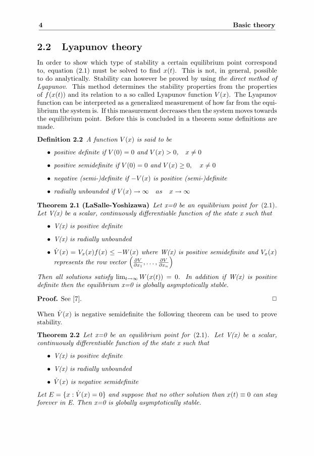
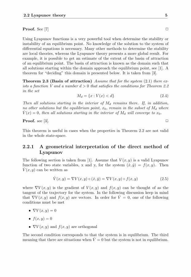
The function V (x, y) can be plotted as curves in the xy-plane. These curves areknown as level curves. Figure 2.1 shows two level curves for the Lyapunov function.One for V (x, y) = c1 and one for V (x, y) = c2 where c2 > c1 > 0. The gradient∇V (x, y), f(x, y) and the angle, θ, between them are also shown together with thetrajectory of the system. The following discussion is based on this figure.
Assume the origin to be the goal state, i.e. the equilibrium point. A correctlydesigned Lyapunov function will then have a gradient which is pointing away fromthe origin as shown in figure 2.1. Equation (2.5) is a scalar product and it followsfrom the definition of scalar products that in order for V (x, y) ≤ 0, the angle θbetween f(x, y) and the gradient must be in the range [π/2, 3π/2]. This means thatf(x, y) must be pointing inwards with respect to V (x, y) = c1 or at worst tangentto this curve. Since f(x, y) represents the direction of motion of the system, itmoves inwards. It will then meet another level curve and if V (x, y) < 0 the systemcontinues to move inwards. This is repeated until it reaches the origin. From thisdiscussion it follows that a trajectory starting inside c2 will never cross the curveV (x, y) = c2 and thus c2 makes up the outer limit for the basin of attraction forthis trajectory.
∇ V ( x,y)
f ( x,y)
V ( x,y) =c2
V ( x,y) =c1
x
y
θ
Figure 2.1. Geometrical interpretation of the Lyapunov functions. The figure shows thegradient, f(x, y) and the angle θ between them. The shaded curve is the trajectory of thesystem.
2.3 Lyapunov theory and control design 7
2.3 Lyapunov theory and control design
In the previous section it was shown that if a Lyapunov function is found so that itstime derivative is negative definite within an area, all trajectories starting withinthat area will converge to same equilibrium point. How can closed loop systems bedesigned so that they have this property?
Consider the systemx = f(x, u) (2.6)
We would like to find a control law u = k(x) which makes some desired state of theclosed loop system asymptotically stable. By picking a Lyapunov function, V (x),and choosing k(x) so that
V = Vxf(x, k(x)) = −W (x) (2.7)
(where W (x) is positive definite) closed loop stability is given by Theorem 2.1. It isnot obvious how V (x) and W (x) should be chosen. To make it easier the followingdefinition is of interest.
Definition 2.3 (Control Lyapunov Function) A smooth, positive definite, ra-dially unbounded function V (x) is called a control Lyapunov function(clf) for (2.6)if for all x �= 0,
V = Vxf(x, u) < 0 for some u (2.8)
A theorem known as Artstein’s theorem has been developed to make the clf mean-ingful. The theorem says that the existence of a clf is equivalent to the existenceof a control law which will make the desired state global asymptotically stable, see[4].

8 Basic theory
Chapter 3
Backstepping
In the previous chapter the theory which backstepping is based upon was presen-ted. There, the need of a control lyapunov function (clf) was shown. It was statedthat if a clf exists, a control law which make the system globally asymptoticallystable can be found. However, no clue to how to find a clf or the control law wasgiven. Backstepping is a procedure which finds both a clf and a control law simul-taneously and is the topic of this chapter.
First, a description of the backstepping design procedure is given. Then differ-ent aspects of the design, such as different design choices and which type of systemthat can be handled, is considered.
3.1 Backstepping design procedure
To show how to find a clf and a control law, a short design example is considered.It is a variant of a design example presented in [7]. The system that is to becontrolled is given below
x =f(x) + g(x)ξ
ξ =a(x, ξ) + b(x, ξ)u(3.1)
where x ∈ Rn and ξ ∈ R are state variables and u ∈ R is the control input.
First ξ is regarded as a control input for the x-subsystem. ξ can be chosen inany way to make the x-subsystem globally asymptotically stable. The choice is de-noted ξdes(x) and is called a virtual control law. For the x-subsystem a clf, V1(x),can be chosen so that with the virtual control law inserted its time derivativebecomes negative definite.
V1(x) = V1xx = V1x(x)(f(x) + g(x)ξdes(x)
)< 0, x �= 0 (3.2)
9
10 Backstepping
A new state is introduced which represents the residual ξ = ξ−ξdes(x). The system(3.1) is then written in terms of these new variables, resulting in
x =f(x) + g(x)(ξ + ξdes(x))
˙ξ =a(x, ξ + ξdes(x)) + b(x, ξ + ξdes(x))u − ∂ξdes(x)
∂x
(f(x) + g(x)(ξ + ξdes(x))
)
(3.3)
For the system (3.3) a clf is constructed from V1(x) by adding a quadratic termwhich penalizes the residual ξ, V2(x, ξ) = V1(x) + 1
2 ξ2. Differentiating V2(x, ξ)w.r.t. time yields
V2(x, ξ) =V1x(x)(f(x) + g(x)ξdes(x) + g(x)ξ
)+ ξ
(a(x, ξ + ξdes(x))
)+
ξ
(b(x, ξ + ξdes(x))u − ∂ξdes(x)
∂x
(f(x) + g(x)(ξ + ξdes(x))
)) (3.4)
Equation (3.4) can be rewritten in the following way if the variables that thefunctions depend on are omitted.
V2 =V1x(f + gξdes)+
ξ
(V1xg + a + bu − ∂ξdes
∂x
(f + g(ξ + ξdes)
)) (3.5)
To guarantee stability V2 has to be negative definite. This can be achieved bychoosing the control input, u in (3.5) as
u =1b
(∂ξdes
∂x
(f + g(ξ + ξdes)
)− a − V1g − kξ
), k > 0 (3.6)
Then V2 becomesV2 = V (f + gξdes) − kξ2 ≤ 0 (3.7)
If u is not the actual control input but a virtual control law consisting of statevariables, then the system can be further expand by starting over again. Hence thebackstepping design procedure is recursive.
3.2 Aspects on backstepping
3.2.1 Design choices
When deriving a control law using backstepping many variations can be done.Among other opportunities this enables the designer to benefit from useful non-linearities. With useful means that the nonlinear terms naturally stabilizes thesystem. This is done by choosing the virtual control laws properly. For examplessee [4].
3.2 Aspects on backstepping 11
Another design choice is using a non-quadratic clf. To render equation (3.4) neg-ative definite, u was chosen so that it canceled some dynamics,
∂ξdes
∂x
(f + g(ξ + ξdes)
), a, V1xg
and replaced them with linear dynamics (−kξ). Some of these terms may insteadbe canceled by choosing V1x(x) properly. This is done by not deciding what V1x(x)should look like until the expression corresponding to V2 has been derived. Whichdynamics that V1x(x) can cancel and still be a valid clf for the x-subsystem is theninvestigated. This design choice usually results in improved robustness and is usedlater in Chapter 5.
3.2.2 Which system can be handled
To be able to apply backstepping to a system, it must have a so called lowertriangular form. Pure-feedback form systems (3.8) is one example of this form.
x =f(x, ξ1)
ξ1 =g1(x, ξ1, ξ2)...
ξi =gi(x, ξ1, . . . , ξi, ξi+1)...
ξm =gm(x, ξ1, . . . , ξm, u)
(3.8)
Also systems which can be written on strict-feedback form (3.9) can be handled.
x =f(x) + g(x)ξ1
ξ1 =f1(x, ξ1) + g1(x, ξ1)ξ2
...
ξi =fi(x, ξ1, . . . , ξi) + gi(x, ξ1, . . . , ξi)ξi+1
...
ξm =fm(x, ξ1, . . . , ξm) + gm(x, ξ1, . . . , ξm)u
(3.9)
Many physical systems can not be written on a lower triangular form. However, byneglecting some physical properties when modeling the system, it can be written onthis form. Then it is possible to apply the backstepping technique. Of course someform of analysis or simulation have to be carried out to verify that the neglectedphysical property does not affect the stability of the closed loop system.

12 Backstepping
Chapter 4
The missile
To be able to derive a controller, it is necessary to have a model of the systemwhich is to be controlled. The better the model is, the bigger the chances are thatthe closed loop system will have some desired properties. On the other hand, avery detailed model will be complex and it can be hard to find a controller.
In this chapter a model describing the missile dynamics is derived in section 4.2.A short presentation of the missile is first given in section 4.1, including someimportant definitions.
4.1 Introduction to the missile
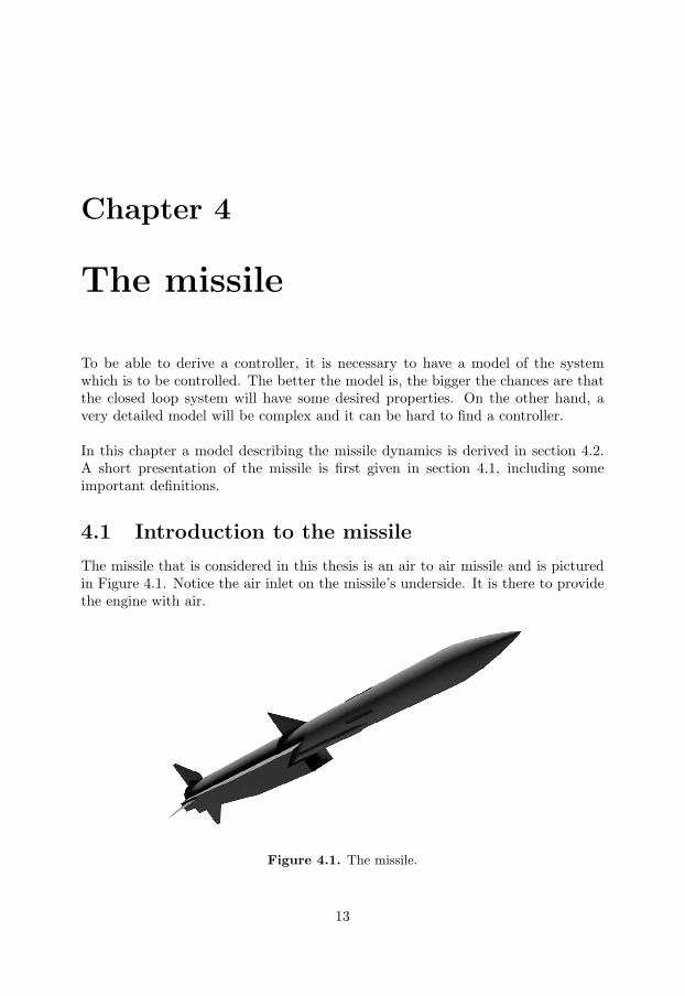
The missile that is considered in this thesis is an air to air missile and is picturedin Figure 4.1. Notice the air inlet on the missile’s underside. It is there to providethe engine with air.
Figure 4.1. The missile.
13
14 The missile
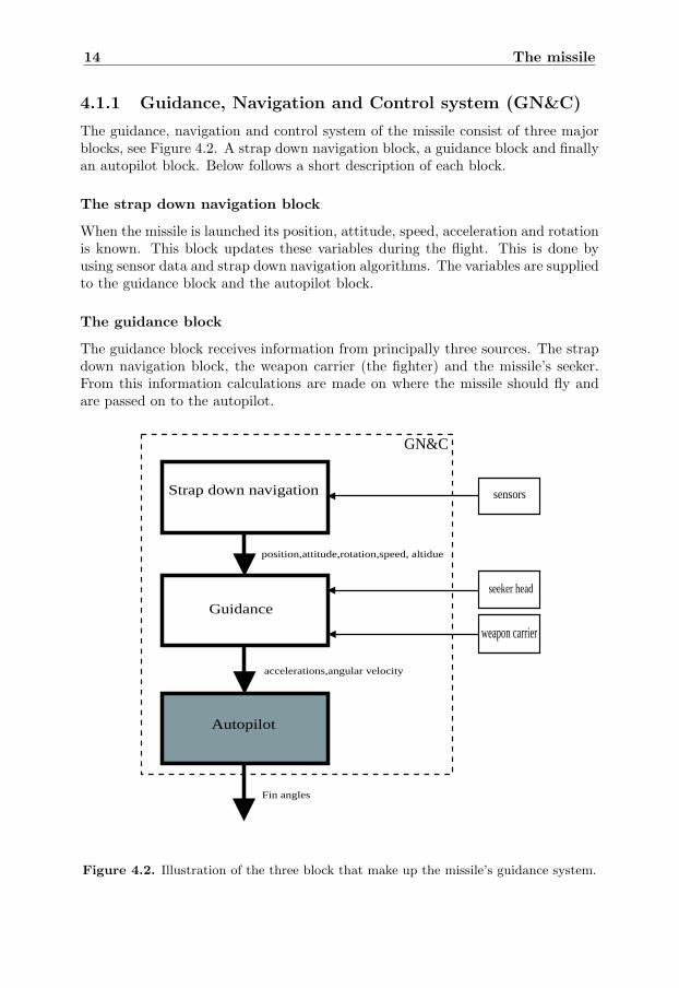
4.1.1 Guidance, Navigation and Control system (GN&C)
The guidance, navigation and control system of the missile consist of three majorblocks, see Figure 4.2. A strap down navigation block, a guidance block and finallyan autopilot block. Below follows a short description of each block.
The strap down navigation block
When the missile is launched its position, attitude, speed, acceleration and rotationis known. This block updates these variables during the flight. This is done byusing sensor data and strap down navigation algorithms. The variables are suppliedto the guidance block and the autopilot block.
The guidance block
The guidance block receives information from principally three sources. The strapdown navigation block, the weapon carrier (the fighter) and the missile’s seeker.From this information calculations are made on where the missile should fly andare passed on to the autopilot.
Strap down navigation
Guidance
Autopilot
position,attitude,rotation,speed, altidue
accelerations,angular velocity
Fin angles
sensors
seeker head
weapon carrier
GN&C
Figure 4.2. Illustration of the three block that make up the missile’s guidance system.
4.1 Introduction to the missile 15
The autopilot
The autopilot receives information from the guidance block on where the missileshould fly. This information is expressed in terms of demanded directional acceler-ations and angular velocities . The task of the autopilot is to fulfill that the missilereceives the wanted accelerations and angular velocities. It also receives measuredaccelerations and angular velocities from the strap down navigation block that areused for feed-back when calculating the fins deflections. This thesis treats how thisis done.
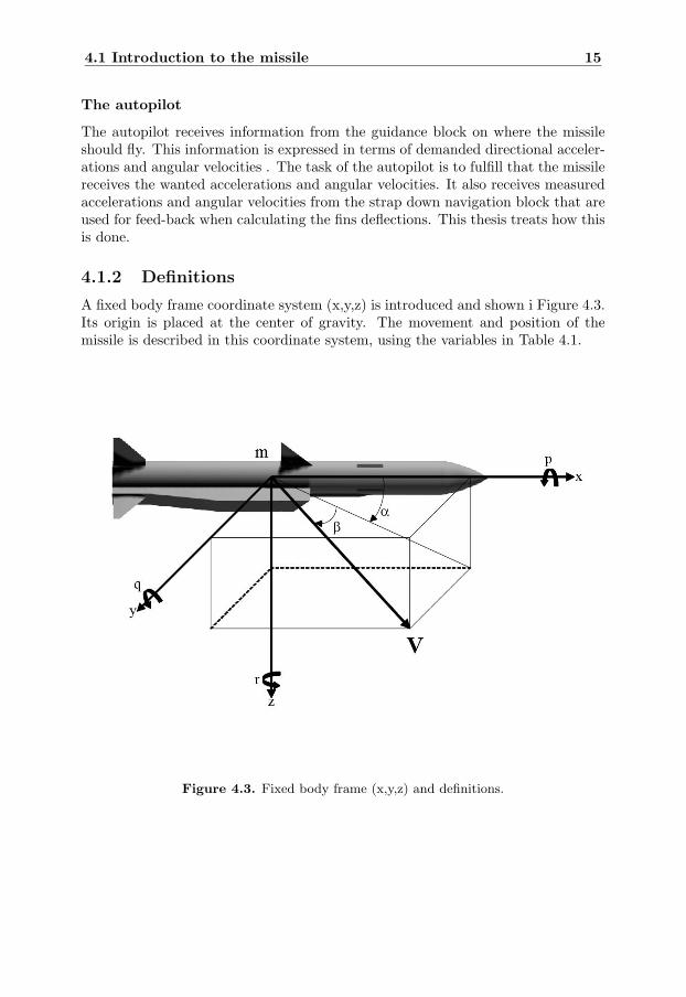
4.1.2 Definitions
A fixed body frame coordinate system (x,y,z) is introduced and shown i Figure 4.3.Its origin is placed at the center of gravity. The movement and position of themissile is described in this coordinate system, using the variables in Table 4.1.
Figure 4.3. Fixed body frame (x,y,z) and definitions.
16 The missile
x, y, z fixed body frame coordinatesV speed vector
p, q, r angular velocities round the (x,y,z)-axisα angle of attackβ side slip anglem mass of the missile
Table 4.1. Explanation of the variables given in Figure 4.3.
The velocity vector is divided into three components as explained below.
u = speed component of the center of gravity in the x-direction
v = speed component of the center of gravity in the y-direction
w = speed component of the center of gravity in the z-direction
In the thesis the following terms are also used.
roll-channel, is used to describe actions that give rise to movement round thex-axis.
pitch-channel, to describe movement round the y-axis.
yaw-channel, movement round the z-axis.
4.1.3 Maneuvering
To steer the missile, movement in the roll, pitch and yaw-channels are generated.In the pitch-channel the variables that are to be controlled are the acceleration inthe z-direction and the pitch rate q. The angle of attack α is closely related tothese variables and appears naturally in the equations which describes the pitch-dynamics.
In the yaw-channel the typical goal is to keep β small. The reason for this is,a large value can lead to that the engine does not get enough air and goes out. Fora very short period β is allowed to have large values. When the missile is very closeto its target the overall goal is to hit that target. In order to do that it may requirea β that is so large that the engine dies. The variables to control here are the ac-celeration in the y-direction or the yaw rate r. These have a strong connection to β.
It is possible to rotate the missile either round the x-axis or the velocity vectorV. When rotating round V, α and β are unchanged. It is possible to write thecontroller so that a rotation always is done round the velocity vector. In this thesisthis possibility is not used. Instead it always rotates round the x-axis but by sim-ultaneously create a movement in the yaw-channel rolling round V can be achieved.
This missile is a bank to turn missile. It means that it turns by first rolling followed
4.2 Deriving a model of the missile 17
by an acceleration in the negative z-direction, pitch-channel. The reason for this isthe placement of the air inlet. By performing a turn this way the side slip angle,β, is kept small so that the engine can be provided with air. The placement of theair inlet also restricts the maneuvering in the pitch channel. The acceleration inthe positive z-direction must not be larger than 50 m
s2 . So if the missile is flyingstraight forward and a strong dive is desired the missile must first roll over on itsback followed by an acceleration in the negative z-direction.
4.1.4 Actuator dynamics
A servo sets the desired fin deflections. This has the following dynamics [5].
δ =ω2
0
s2 + 2ζω0s + ω20
δa,e,r (4.1)
Here ω0 = 250 and ζ = 0.7. This gives poles in −175 ± 178.54i.
4.2 Deriving a model of the missile
In this section a model of the missile is derived. First a theoretical backgrounddescribing some basic rigid body dynamics, see [8], is given followed by a sectiondescribing the assumptions. Then the actual model is derived.
4.2.1 Basic rigid body dynamics
The relationship between the sum of all forces,∑
F acting on a body and itsinertial acceleration, a, is given by the well known Newton’s second law.
Definition 4.1 (Newton’s second law)
∑F = ma = m
d
dtv (4.2)
Here v represents the velocity vector. The next definition is also very useful.
Definition 4.2 (Euler’s equation)
∑M = H =
d
dtIω (4.3)
Euler’s equation states that the moment of all forces acting on a body equals theinertial time rate of change of angular momentum of the body.
The two definitions above involves a time derivate of a vector in the inertial frame.The inertial frame is in this application the earth and is considered fixed. Whena body frame rotates relatively a fixed frame the following theorem is used tocalculate the derivate of a vector expressed in the fixed frame.
18 The missile
Theorem 4.1 (Time derivate of a vector in a rotating frame) Let XYZrepresent the fixed frame, xyz the body frame and ωxyz the angular velocity of thebody. Then the time derivate of a vector V is
(dVdt
)
XY Z
=(
Vdt
)
xyz
+ ωxyz × V (4.4)
Proof. see [8]. �
The moment of inertia matrix, I is a part of Euler’s equation. In this case whenthe origin of the body’s frame is placed in the body’s center of gravity the matrixI equals the principal axis frame showed below.
I =
Ixx 0 00 Iyy 00 0 Izz
(4.5)
4.2.2 Assumptions
The following assumptions are made when the model is derived. Some consequencesof these assumptions are also outlined.
• Assumption 1: The thrust and torque produced by the engine are neglected.The air resistance is also neglected.
• Assumption 2: The effect of gravity is neglected.
• Assumption 3: Small values of α and β are assumed.
• Assumption 4: The velocity in the x-direction, u is constant.
• Assumption 5. The fin servo dynamics are much faster than the dynamicsin the roll, pitch and yaw-channels. This dynamics are therefore not includedin the model.
Assumption 3 means that sinα ≈ α, tanα ≈ α and cosβ ≈ β. Also u ≈ V holdsdue to this assumption. Together with the geometric relations given in Figure 4.3the following can be stated
α =w
u, β =
v
|V | =v
u
From assumption 4 it follows that u = 0.
The assumptions are made to simplify the model.
4.2 Deriving a model of the missile 19
4.2.3 Equations
Force equations
Since the effect of gravity and the thrust are neglected the only forces acting onthe missile are aerodynamic forces Fa.
Fa = −qdS
CT
CC
CN
(4.6)
Here qd is the dynamic pressure S is a reference area. CT , CC and CN are shortnotations for the following expressions.
CT =1CC =CCββ + CCδr
δr
CN =CNαα + CNδeδe
(4.7)
δe is the elevator deflection and δr is the rudder deflection. The CC-coefficients andthe CN -coefficients are explained in section 4.2.5. From definition 4.1 and theorem4.1 it follows that
F = m( ˙V + ω × V ) = m
uvw
+
pqr
×
uvw
(4.8)
Replacing F in (4.8) with (4.6) together with (4.7) yields the following
−qdS =m(u + qw − vr) (x-direction)−qdS(CCββ + CCδr
δr) =m(v − pw + ur) (y-direction)−qdS(CNαα + CNδr
δr) =m(w + pv − qu) (z-direction)(4.9)
Using assumption 4, u = 0, the equation in the x-direction becomes a static re-lationship which means there are no dynamics that have to be modeled in thisdirection. Using assumption 3 and assumption 4 again, the equation in the y-direction can be written.
−qdS(CCββ + CCδrδr) =m
(d
dt(uβ) − pαu + ur
)
=um(β − pα + r
)
=V m(β − pα + r
)(4.10)
The equation in z-direction can also be rewritten using assumption 3 and assump-tion 4.
−qdS(CNαα + CNδrδr) =m
(d
dt(uα) + pβu − qu
)
=um (α + pβ − q)=V m (α + pβ − q)
(4.11)
20 The missile
Finally equation (4.10) and equation (4.11) are rewritten.
β =pα − r − qdS
V m(CCββ + CCδr
δr) (y-direction)
α = − pβ + q − qdS
V m(CNαα + CNδr
δr) (z-direction)(4.12)
Momentum equations
The aerodynamic momentums, Ma, that affect the missile are written
Ma = qdSd
Cl
Cm
Cn
(4.13)
where d is a reference length, here the diameter of the missile. Cl, Cm and Cn areshort notations for
Cl =Clββ + Clpd
2Vp + Clδa
δa
Cm =Cmαα + Cm|β||β| + Cmqd
2Vq + Cmδeδe
Cn =Cnββ + Cnαβαβ + Cnrd
2Vr + Cnδa
δa + Cnδrδr
(4.14)
Euler’s equation together with equation (4.1), (4.5) and Theorem 4.1 forms thefollowing momentum equations for the missile
M =
Ixx 0 00 Iyy 00 0 Izz
pqr
+
pqr
×
Ixx 0 00 Iyy 00 0 Izz
pqr
=
Ixxp + qr (Izz − Iyy)Iyy q + pr (Ixx − Izz)Izz r + pq (Iyy − Ixx)
(4.15)
Inserting equation (4.13) and (4.14) into (4.15) yields
p =1
Ixx
qr (Iyy − Izz)︸ ︷︷ ︸
=0
+qdSd
(Clββ + Clp
d
2Vp + Clδa
δa
)
q =1
Iyy
(pr (Izz − Ixx) + qdSd
(Cmαα + Cm|β||β| + Cmq
d
2Vq + Cmδeδe
))
r =1
Izz
(pq (Ixx − Iyy) + qdSd
(Cnββ + Cnαβαβ + Cnr
d
2Vr + Cnδa
δa + Cnδrδr
))
(4.16)
Since the missile is symmetric, Iyy = Izz, the qr (Iyy − Izz)-term in the p equationequals zero.
4.2 Deriving a model of the missile 21
4.2.4 State-space representation
Equation (4.12) and equation (4.16) make up a set of equations that describes themissile dynamics. The system can be written on the state-space representation
x =f(x) + g(x)uy =h(x)
(4.17)
where
x =
pqrα
β
(4.18)
f(x) =
qdSdIxx
(Clββ + Clp
d2V p
)1
Iyy
(pr (Izz − Ixx) + qdSd
(Cmαα + Cm|β||β| + Cmq
d2V q
))1
Izz
(pq (Ixx − Iyy) + qdSd
(Cnββ + Cnαβαβ + Cnr
d2V r
))−pβ + q − qdS
V m (CNαα)pα − r − qdS
V m (CCββ)
(4.19)
g(x)u =
qdSdIxx
Clδaδa
qdSdIyy
Cmδeδe
qdSdIzz
Cnδaδa + qdSdCnδr
Izzδr
qdSV mCNδe
δeqdSV mCCδr
δr
(4.20)
h(x) =
pqrαβ
(4.21)
4.2.5 Comments about the aerodynamic coefficients
Here follows a short explanation of the aerodynamic coefficients CT , CC , CN , Cl, Cm
and Cn. The side force coefficient CC = CCββ +CCδrδr is taken as an example. It
is build up by a term depending on the side slip angle, β, and a term depending onfin deflection δr. CCβ and CCδr
are known as aerodynamic derivatives and definesthe side force curve slope in relation to β (∂Cc
∂β ) and δ (∂Cc
∂δr), also see [6]. The value
of this derivative changes with the speed according to Table B.1 in appendix B.Usually these values are marred with uncertainties. This is, among other reasons,because it is hard to model aerodynamics correctly. In this thesis, when referredto the aerodynamic coefficients it is the aerodynamic derivatives that is though ofif nothing else is said.
22 The missile
4.2.6 The simulation model
The model that has been derived in this chapter is only used to find the controller.When simulations are performed a more complex model of the missile is used tocalculate the missile dynamics. This model does not use the assumptions stated insection 4.2.2 to the same extend and is a more realistic model of the true missile.Data on the missile used in the simulation is found in Appendix A. The simulationenvironment is implemented in ADA.
Chapter 5
Backstepping design for themissile
In this chapter control laws for the missile are derived using backstepping. First thecontrol objectives are described, then the control laws are derived. This is followedby a section which considers aspects of the design, including a short robustness dis-cussion. In section 5.3.4 some design flexibilities are explored and finally simulationresults are presented.
5.1 Control objectives
The control objectives are that the missile should follow reference signals given inthe roll, pitch and yaw-channel. The reference signals in the pitch and yaw channelare expressed as directional accelerations while in the roll channel it is expressed asan angular velocity. If the notation az is used for directional acceleration along thez-axis and ay for directional acceleration along the y-axis, the control objectivescan be expressed as
p =pref (roll)
az =arefz (pitch)
ay =arefy (yaw)
5.1.1 Conversion of the accelerations
Since ay and az are not states in the state-space model, described by equations(4.18)-(4.21), they can not be used directly in the design. First they need to beconverted into α and β. To find this conversion the force equation in y-directionand z-direction are used, see equation (4.9). The reference signals, aref
z and arefy ,
are expressed in terms of the missile’s own coordinate system. Therefore the part
23
24 Backstepping design for the missile
which arises from the rotation of the velocity vector, the (ω×V )-term, is neglectedand equation (4.9) can be written (with v = ay and u = az)
ay = − qdS
m(CCββ + CCδr
)
az = − qdS
m(CNαα + CNδe
)(5.1)
Here δe and δr are the elevator and rudder deflection, respectively. From equation(5.1) β and α can be separated.
α =
(− azm
QdS − CNδeδe
)
CNα(5.2)
β =
(−aym
QdS − CCδrδr
)
CCβ(5.3)
This conversion form az to α and ay to β involve the fin deflections and can beregarded as a form of feedback. Simulations that has been performed showed thatthe missile can become instable due to this feedback. Therefore the δr and δe termsin equation (5.1) is replaced with an approximation. This approximation is derivedbelow.
Start with the expressions for the momentum equation in the y and z directions,see equation (4.16).
Iz q =QdSd(Cmαα + Cmδeδe + f(β, q, p, r))
Iy r =QdSd(Cnββ + Cnαβαβ + Cnδrδr + g(α, q, p, r))
(5.4)
Equilibrium is assumed and the contribution from f and g are neglected to makethe conversion independent the other states variables. The equations may then bewritten as
δe = − Cmαα
Cmδe
δr = − Cnββ + Cnαβαβ
Cnδr
(5.5)
Inserting the expression for δe and δr in equation (5.2) respectively (5.3) finallyyields the following expression for converting the accelerations into angles
α = − maz
QdS(CNα − CNδe Cmα
Cmδe
)
β = − may
QdS(CCβ − CCδr (Cnβ+Cnαβα)
Cnδr
)(5.6)
5.2 Backstepping design 25
5.2 Backstepping design
In this section backstepping design is used to derive control laws for the missile.The design follows the ideas given in Chapter 7.2 in [7]. The first thing that has tobe done is to make the state space model applicable to backstepping. In the state-space model, described by equations (4.17)-(4.21), the control inputs are presentin all states and the system is not written on lower triangular form. Therefore itis not possible perform backstepping design. However, if the force contributions ofthe fins are neglected the system is on the correct form for backstepping design.This assumption is valid since the coefficients CNδe
and CCδrare quite small in
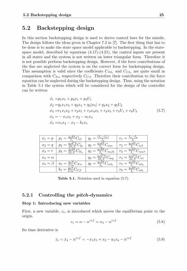
comparison with CNα respectively CCβ . Therefore their contribution to the forceequation can be neglected during the backstepping design. Thus, using the notationin Table 5.1 the system which will be considered for the design of the controllercan be written
x1 =p1x5 + p2x1 + p3U1
x2 =q1x1x3 + q2x4 + q3|x5| + q4x2 + q5U2
x3 =r1x1x2 + r2x5 + r3x4x5 + r4x3 + r5U1 + r6U3
x4 = − x1x5 + x2 − a1x4
x5 =x1x4 − x3 − b1x5
(5.7)
x1 = p p1 = qddSIx
Clβ q1 = (Iz−Ix)Iy
r1 = Ix−Iy
Iz
x2 = q p2 = qdd2S2IxV Clp q2 = qddS
IyCmα r2 = qddS
IzCnβ
x3 = r p3 = qddS2IxV Clδa
q3 = qddSIy
Cm|β| r3 = qddSIz
Cnαβ
x4 = α q4 = qdd2S2IyV Cmq r4 = qdd2S
2IzV Cnr
x5 = β a1 = qdSV mCNα q5 = qddS
IyCmδe
r5 = qddSIz
Cnδa
b1 = qdSV mCCβ r6 = qddS
IzCnδr
Table 5.1. Notation used in equation (5.7).
5.2.1 Controlling the pitch-dynamics
Step 1: Introducing new variables
First, a new variable, z1, is introduced which moves the equilibrium point to theorigin.
z1 = α − αref = x4 − αref (5.8)
Its time derivative is
z1 = x4 − αref = −x1x5 + x2 − a1x4 − αref (5.9)
26 Backstepping design for the missile
Rewriting equation (5.8) using x4 = z1 + αref and inserting into equation (5.9)yields
z1 = x4 − αref = −x1x5 + x2 − a1z1 − a1αref − αref (5.10)
From equation (5.10) we can see that the state x2 can be regarded as a control inputfor the z1-dynamics. In physical properties this means that the pitch-dynamics iscontrolled with the pitch rate, which make sense. The desired value of x2 is thevirtual control law and is denoted, xdes
2 . It is chosen such that it will give thez1-dynamics some desired properties.
xdes2 = x1x5 + a1α
ref + αref − k1z1 (5.11)
Here k1 is a design parameter which is determined later. The next step is tointroduce the residual x2-xdes
2 , which is denoted z2.
z2 = x2 − xdes2 = x2 − x1x5 − a1α
ref − αref + k1z1 (5.12)
The pitch-dynamics are written in terms of z1 and z2.
z1 = − (a1 + k1)z1 + z2
z2 =(−k21 − k1a1 − k1q4 + q2 − x2
1)z1 + (k1 + q4)z2
+ (q1 + 1)x1x3 + q3 |x5| + (q4 + b1 − p2)x1x5 − αrefx21 − p1x
25
+ (q2 + q4a1)αref + (q4 − a1)αref − αref
+ q5U2 − p3x5U1
(5.13)
The first equation in (5.13) leads to a constraint on k1,
k1 > −a1 (5.14)
in order for the z1-dynamics to be stable. Using the following notations,
ϕ1(x) =(q1 + 1)x1x3 + q3 |x5| + (q4 + b1 − p2)x1x5 − αrefx21 − p1x
25
A =(q2 + q4a1)αref + (q4 − a1)αref − αref
equation (5.13) can be rewritten in a more compact form
z1 = − (a1 + k1)z1 + z2
z2 =(−k21 − k1a1 − k1q4 + q2 − x2
1)z1 + (k1 + q4)z2
+ ϕ1(x) + A + q5U2 − p3x5U1
(5.15)
Step 2: Finding the clf
A non-quadratic clf for the system (5.15) is selected as
V (z1, z2) = F (z1) +12z22 (5.16)
5.2 Backstepping design 27
where F (z1) is any valid clf for the z1-dynamics which is determined below. Dif-ferentiating the clf w.r.t. time yields
V (z1, z2) = − F ′(z1)(a1 + k1)z1
+ z2[F ′(z1) + z1(−k21 − k1(a1 + q4) + q2 − x2
1)+ z2(q4 + k1) + ϕ1(x) + A + q5U2 − p3x5U1]
(5.17)
The complexity of the z2-dynamics may be reduced by selecting F ′(z1) so that itcancels the z1-dynamics inside the []-brackets. By picking F ′(z1) as
F ′(z1) = −z1(−k21 − k1(a1 + q4) + q2 − x2
1) (5.18)
this is achieved. In order for the first term in (5.17) to be negative definite, F ′(z1)must lie in the 1st or 3rd quadrant. This constraint means that F ′(z1) = −z1(−k2
1−k1(a1 + q4) + q2 − x2
1) > 0 which is the same as
−k21 − k1(a1 + q4) + q2 − x2
1 < 0 (5.19)
⇔k21 + k1(a1 + q4) − q2 + x2
1 > 0 (5.20)
Since k1 is a design parameter it can be adjusted so that inequality (5.20) alwaysholds. To be able to determine the value of k1 some knowledge about the coefficientsa1, q2 and q4 are necessary. It is known that:
• q2 < 0, always
• (a1 + q4) > 0, always
This, and the fact that the term x21 always is greater or equal to zero, gives the
following constraints on k1
k1 > 0, k1 ∈ R (5.21)
Earlier it was also stated that k1 > −a1, which still must hold.
Step 3: Determine the control input
Inserting the selected F ′(z1) , equation (5.18), into (5.17) yields
V (z1, z2) = − (−k21 − k1(a1 + q4) + q2 − x2
1)(a1 + k1)z21
+ z2 [z2(q4 + k1) + ϕ1(x) + A + q5U2 − p3x5U1](5.22)
in which the first term is negative definite as long as (5.14) and (5.21) holds. Tomake the second term negative definite as well, the control input is used. Choosing
q5U2 − p3x5U1 = −z2k2 − ϕ1(x) − A (5.23)
where k2 is a new design parameter, leads to
V (z1, z2) = (−k21 − k1(a1 + q4) + q2 − x2
1)z21 + (−k2 + k1 + q4)z2
2 (5.24)
For (5.24) to be negative definite, the following constraint on k2 must hold
k2 > (k1 + q4) (5.25)
28 Backstepping design for the missile
5.2.2 Controlling the yaw-dynamics
Step 1: Introducing new variables
First a new variable, z3, is introduced.
z3 = β − βref = x5 − βref (5.26)
It makes the origin the equilibrium point. Differentiating z3 w.r.t. time and re-writing it in terms of z3 results in
z3 = x1x4 − x3 − b1z3 − b1βref − βref (5.27)
In equation (5.27) x3 can be regarded as a control input and the virtual controllaw xdes
3 is chosen as
xdes3 = x1x4 − b1β
ref − βref + k21z3 (5.28)
Let z4 represent the residual
z4 = x3 − xdes3 = x3 − x1x4 + b1β
ref + βref − k21z3 (5.29)
Writing the yaw -dynamics in terms of z3 and z4 yields
z3 = − (b1 + k21)z3 − z4
z4 =(r2 + r3x4 + r4k21 + x21 − x4p1 + k21b1 + k2
21)z3 + (r4 + k21)z4
+ r1x1x2 + r3x4βref + r4x1x4 + x2
1βref − x1x2 + a1x1x4 − p2x1x4
+ r2βref − r4b1β
ref − p1x4βref − r4β
ref + brβref + βref
+ (r5 − p3x4)U1 + r6U3
(5.30)
As with the pitch-dynamics the first equation in (5.30) gives a constraint on k21,
k21 > −b1 (5.31)
to make the z3-dynamics stable. The second equation may be written in morecompact manner.
z3 = − (b1 + k21) − z4
z4 =(r2 + r3x4 + r4k21 + x21 − x4p1 + k21b1 + k2
21)z3 + (r4 + k21)z4
+ ϕ2(x) + B + (r5 − p3x4)U1 + r6U3
(5.32)
Here the following notations were used.
ϕ2(x) =r1x1x2 + r3x4βref + r4x1x4 + x2
1βref − x1x2 + a1x1x4 − p2x1x4
B = + r2βref − r4b1β
ref − p1x4βref − r4β
ref + brβref + βref
(5.33)
5.2 Backstepping design 29
Step 2: Finding the clf
Now a clf for (5.32) can be found. The benefit of picking a non-quadratic clf isonce again used.
V22(z3, z4) = G(z3) +12z24 (5.34)
where G(z3) is any valid clf for the z3-dynamics. Differentiating V22(z3, z4) w.r.t.time yields
V22(z3, z4) = − G′(z3)(k21 + b1)z3
+ z4[−G′(z3) + z3(r2 + r3x4 + r4k21 + x21 − x4p1 + k21b1 + k2
21)+ z4(r4 + k21) + ϕ2(x) + B + (r5 − p3x4)U1 + r6U3]
(5.35)
The first term in (5.35) tells that G′(z3) must lie in the 1st or 3rd quadrant torender it negative definite. This corresponds to G′(z3) > 0. In the second term,describing the z4-dynamics, one would like to cancel the z3-dynamics by choosingG′(z3) as
G′(z3) = (r2 + r3x4 + r4k21 + x21 − x4p1 + k21b1 + k2
21)z3 (5.36)
Since G′(z3) > 0, the following inequality must hold
(r2 + r3x4 + r4k21 + x21 − x4p1 + k21b1 + k2
21) > 0
⇔k221 + k21(r4 + b1) + r2 + x2
1 + (r3 − p1)x4 > 0 (5.37)
k21 ∈ R, but when x4 < 0 k21 becomes a complex number. Therefore the x4-termcan not be canceled by G′(z3). A new G′(z3) is chosen by simply omitting thex4-terms in (5.36).
G′(z3) = (r2 + r4k21 + x21 + k21b1 + k2
21)z3 (5.38)
This leads to a new constraint on k21
k221 + k21(r4 + b1) + r2 + x2
1 > 0 (5.39)
When examine what values of k21 which will satisfy (5.39) the following knowledgeis used
• x21 > 0, always
• r2 ∈]124, 317[
• (r4 + b1) ∈] − 0.5, 0.5[
This indicates that equation (5.39) hold for any k21 > 0, but equation (5.31),k21 > −b1, must be fulfilled as well.

30 Backstepping design for the missile
Step 3: Determine the control input
Inserting (5.38) in (5.35) yields
V22 = − (r2 + r4k21 + x21 + k21b1 + k2
21)z23(k21 + b1)
+ z4[z3(r3 − p1)x4 + z4(r4 + k21) + ϕ2(x) + B + (r5 − p3x4)U1 + r6U3](5.40)
By choosing the control inputs U1 and U3 as
(r5 − p3x4)U1 + r6U3 = −ϕ2 − B − z3(r3 − p1)x4 − z4k22 (5.41)
where k22 is a design parameter, equation (5.40) now becomes
V22 = − (r2 + r4k21 + x21 + k21b1 + k2
21)z23(k21 + b1)
+ (k21 − k22 + r4)z24
(5.42)
It is made positive definite if
k22 > (k21 + r4) (5.43)
5.2.3 Controlling the roll-dynamics
To control the roll-dynamics a simple PI-controller with a term which cancels thep1x5-term is used.
U1 = −Kpe(t) − Ki
∫ t
0
e(τ)dτ − p1x5
p3(5.44)
where e(t) is the control error. In the roll-channel the loop-gain is rather large,around 60 dB, so therefore reasonable values for Kp and Ki are 0.001-0.01.
5.2.4 Combining the control inputs
From the equations (5.23), (5.41) and (5.44) a fairly complicated equation systemcan be derived, which solution provides the control inputs for the whole missile.
q5U2 − p3x5U1 = −z2k2 − ϕ1(x) − A
(r5 − p3x4)U1 + r6U3 = −ϕ2 − B − z3(r3 − p1)x4 − z4k22
U1 = −Kpe(t) − Ki
∫ t
0
e(τ)dτ − p1x5
p3
(5.45)
The solution to the equation system is
U1 = −Kpe(t) − Ki
∫ t
0
e(τ)dτ − p1x5
p3
U2 =p3x5U1 − z2k2 − ϕ1(x) − A
q5
U3 =−(r5 − p3x4)U1 − ϕ2 − B − z3(r3 − p1)x4 − z4k22
r6
(5.46)
5.3 Aspects on the design 31
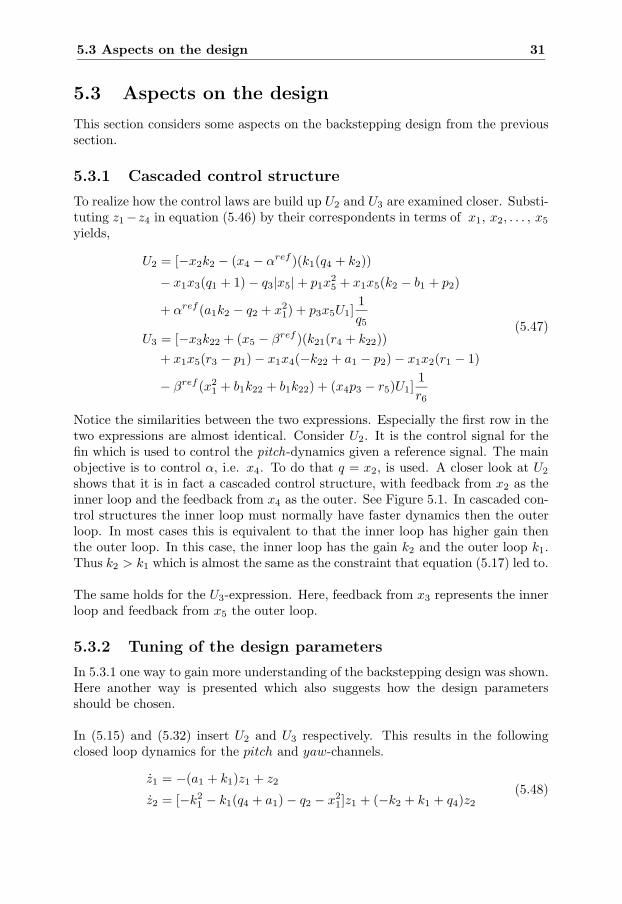
5.3 Aspects on the design
This section considers some aspects on the backstepping design from the previoussection.
5.3.1 Cascaded control structure
To realize how the control laws are build up U2 and U3 are examined closer. Substi-tuting z1−z4 in equation (5.46) by their correspondents in terms of x1, x2, . . . , x5
yields,
U2 = [−x2k2 − (x4 − αref )(k1(q4 + k2))
− x1x3(q1 + 1) − q3|x5| + p1x25 + x1x5(k2 − b1 + p2)
+ αref (a1k2 − q2 + x21) + p3x5U1]
1q5
U3 = [−x3k22 + (x5 − βref )(k21(r4 + k22))+ x1x5(r3 − p1) − x1x4(−k22 + a1 − p2) − x1x2(r1 − 1)
− βref (x21 + b1k22 + b1k22) + (x4p3 − r5)U1]
1r6
(5.47)
Notice the similarities between the two expressions. Especially the first row in thetwo expressions are almost identical. Consider U2. It is the control signal for thefin which is used to control the pitch-dynamics given a reference signal. The mainobjective is to control α, i.e. x4. To do that q = x2, is used. A closer look at U2
shows that it is in fact a cascaded control structure, with feedback from x2 as theinner loop and the feedback from x4 as the outer. See Figure 5.1. In cascaded con-trol structures the inner loop must normally have faster dynamics then the outerloop. In most cases this is equivalent to that the inner loop has higher gain thenthe outer loop. In this case, the inner loop has the gain k2 and the outer loop k1.Thus k2 > k1 which is almost the same as the constraint that equation (5.17) led to.
The same holds for the U3-expression. Here, feedback from x3 represents the innerloop and feedback from x5 the outer loop.
5.3.2 Tuning of the design parameters
In 5.3.1 one way to gain more understanding of the backstepping design was shown.Here another way is presented which also suggests how the design parametersshould be chosen.
In (5.15) and (5.32) insert U2 and U3 respectively. This results in the followingclosed loop dynamics for the pitch and yaw-channels.
z1 = −(a1 + k1)z1 + z2
z2 = [−k21 − k1(q4 + a1) − q2 − x2
1]z1 + (−k2 + k1 + q4)z2
(5.48)
32 Backstepping design for the missile
Missile−
x1x3 ( q1 + 1) q3x5+ p1x25− −
x1x5( k2 b1+ p2) +αre f(a1k2 q2+ x2
1)+ p3x5U1− −
1q5∑∑∑
x4
αre fk1
x2
( q4 k2)− −++
++ +
+
Figure 5.1. Cascaded control structure
z3 = −(b1 + k21)z3 + z4
z4 = [k221 + k21(r4 + b1) − r2 + x2
1]z3 + (−k22 + k21 + r4)z4
(5.49)
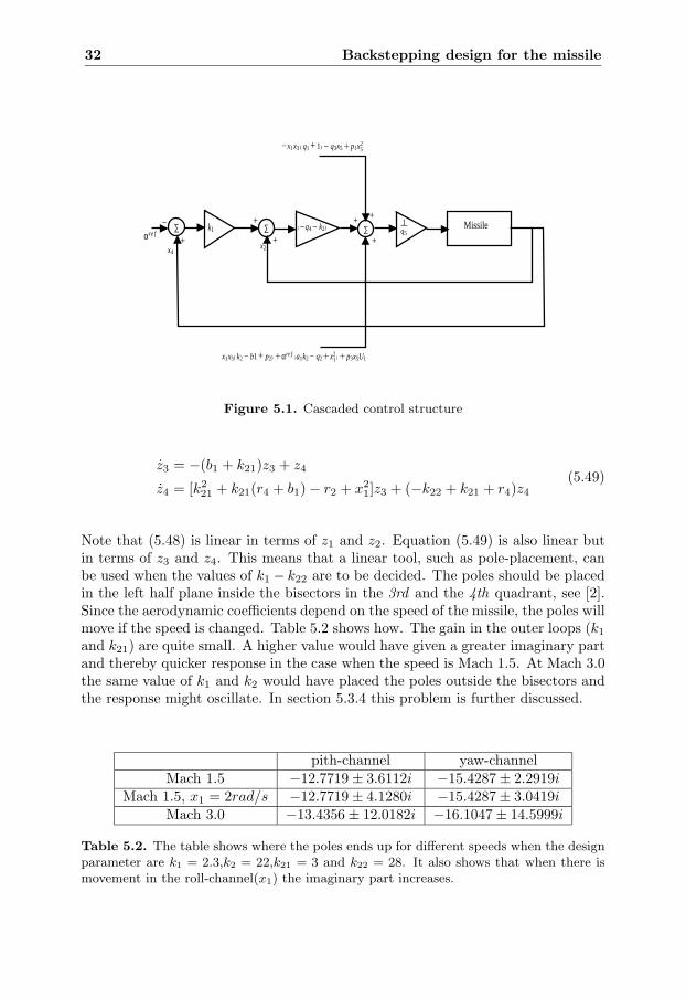
Note that (5.48) is linear in terms of z1 and z2. Equation (5.49) is also linear butin terms of z3 and z4. This means that a linear tool, such as pole-placement, canbe used when the values of k1 − k22 are to be decided. The poles should be placedin the left half plane inside the bisectors in the 3rd and the 4th quadrant, see [2].Since the aerodynamic coefficients depend on the speed of the missile, the poles willmove if the speed is changed. Table 5.2 shows how. The gain in the outer loops (k1
and k21) are quite small. A higher value would have given a greater imaginary partand thereby quicker response in the case when the speed is Mach 1.5. At Mach 3.0the same value of k1 and k2 would have placed the poles outside the bisectors andthe response might oscillate. In section 5.3.4 this problem is further discussed.
pith-channel yaw-channelMach 1.5 −12.7719 ± 3.6112i −15.4287 ± 2.2919i
Mach 1.5, x1 = 2rad/s −12.7719 ± 4.1280i −15.4287 ± 3.0419iMach 3.0 −13.4356 ± 12.0182i −16.1047 ± 14.5999i
Table 5.2. The table shows where the poles ends up for different speeds when the designparameter are k1 = 2.3,k2 = 22,k21 = 3 and k22 = 28. It also shows that when there ismovement in the roll-channel(x1) the imaginary part increases.
5.3 Aspects on the design 33
5.3.3 Robustness of the design
All models of physical systems suffer from model errors and uncertainties. Thismeans that the model on which the design is based differs from the actual physicalsystem. For the missile case the aerodynamic coefficients are an example of suchmodel uncertainties. Sometimes one also has to simplify the model and makeassumptions. In the design, the force contribution from the fins were neglected.Despite that the closed loop system must be stable. In this section the robustnessof the design is therefore studied.
Uncertainties in the aerodynamic coefficients
In equation (5.7) all coefficients p1, p2, . . . , b1 are more or less marred by uncer-tainties. The design led to constraints on k1,k2,k21 and k22 that have a direct con-nection to some of these coefficients. Equation (5.14) gave the constraint k1 > −a1,equation (5.20) showed that k2
1 + k1(a1 − q4) − q2 + x21 > 0 and finally (5.25) said
that k2 > k1. For k21 and k22 similar constraints were found. This gives a directpossibility to design the system so that it is robust against some model uncertain-ties by simply picking the design parameters with a good margin. However, thevalues of k1 − k22 cannot be chosen arbitrary large. The higher the value the moresensitive the system is to disturbances.
Above it was shown that the design could be made robust against some uncer-tainties in the aerodynamic coefficients, namely the ones that appear directly inthe expressions. There are however others that do not appear in the expressions,or they do appear but they enter the design in other ways. These also have to beexamined. Consider equation (5.22)
V (z1, z2) =(−k21 − k1(a1 + q4) + q2 − x2
1)z21
+ z2 [z2(q4 + k1) + ϕ1(x) + A + q5U2 − p3x5U1](5.50)
In the design, q5U2−p3x5U1 = −z2k2−ϕ1(x)−A, was chosen so that it cancels theϕ(x)-term and the A-term. Note that both ϕ(x) and A are made up by aerodynamiccoefficients. What happens if the true values of these coefficients are uncertain.Then V (z1, z2) would not look like the desired equation (5.24). Instead it will looklike
V (z1, z2) =(−k21 − k1(a1 + q4) + q2 − x2
1)z21
+ [(−k2 + k1 + r4)z2 + ∆ϕ1(x) + ∆A] z2
(5.51)
Here ∆ϕ1(x) and ∆A represent the difference between the true values of the coef-ficients and the values that are used in the model. With these extra terms in thez2-term it is much harder to make any comment on the stability properties. Forthe system to be globally asymptotically stable V (z1, z2) must be negative definite.The first term in equation (5.51) is still negative definite, provided that one havetaken good margins against model uncertainties according to what is said in the
34 Backstepping design for the missile
beginning of this section. To make the z2-term negative definite the following mustbe achieved
(−k2 + k1)z22 + ∆ϕ1(x)z2 + ∆Az2 < 0 (5.52)
This is not easy since neither the sign or magnitudes of ∆ϕ1(x) and ∆A are known.The solution to this problem is postpone to the next chapter.
The fact that a non-quadratic clf, F (z1) and G(z3), are used gives us a possib-ility to improve robustness against uncertainties in the aerodynamic coefficients.By the choices of the clf:s the number of terms that includes the coefficients whichthe control inputs have to cancel, were reduced. Instead the coefficients turn upin the constraints for k1, k2, k3 and k4. Here less knowledge about them is neededcompared to what one need in order to cancel them. Using non-quadratic clf:s isone great advantage of Backstepping. This becomes even more clear when dealingwith nonlinearities. In the same manner, as with the uncertainties, you need lessknowledge about the nonlinearities. For examples see [4] and [10].
Force contribution of the fins
In the backstepping design the force contribution of the fins had to be neglected.In the true system the force contributions exists. It is therefore interesting tosee if the design still is globally asymptotically stable. The true system for thepitch-dynamics is
x2 =q1x1x3 + q2x4 + q3x5 + q4x2 + q5U2
x4 = − x1x5 + x2 − a1x4 − a2U2
(5.53)
where a2 is an aerodynamic coefficient. In terms of z1 and z2 equation (5.53) canbe written
z1 = − (a1 + k1)z1 + z2 − a2U2
z2 =(−k21 − k1a1 − k1q4 + q2 − x2
1)z1 + (k1 + q4)z2
+ ϕ1(x) + A + q5U2 − p3x5U1
(5.54)
and the control input U2 is as earlier
U2 =p3x5U1 − z2k2 − ϕ1(x) − A
q5(5.55)
Inserting equation (5.55) into equation (5.54) yields
z1 = − (a1 + k1)z1 + z2
(1 +
k2a2
q5
)− a2
q5(p3x5U1 + ϕ1(x) + A)
z2 =(−k21 − k1 (a1q4) + −x2
1)z1 + (−k2 + k1 + q4)z2
(5.56)
The same non-quadratic clf as in the design is used
V = F (z1) +12z22 (5.57)
5.3 Aspects on the design 35
Differentiating equation (5.57) w.r.t. time and inserting equation (5.56) and yields
V = − F ′(z1)((a1 + k1) z1 − a2
q5(p3x5U1 + ϕ1(x) + A))
+ z2[F ′(z1)a2k2
q5+ (−k2 + k1 + q4)z2]
(5.58)
If F ′(z1) is chosen as earlier the problem of ensuring that V in equation (5.58)is negative definite is similar to the problem that was discussed in the previoussection.
5.3.4 Exploring some design flexibilities
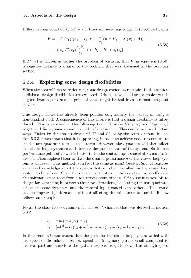
When the control laws were derived, some design choices were made. In this sectionadditional design flexibilities are explored. Often, as we shall see, a choice whichis good from a performance point of view, might be bad from a robustness pointof view.
One design choice has already been pointed out, namely the benefit of using anon-quadratic clf. A consequence of this choice is that a design flexibility is intro-duced. This is explored in the following text. To make V (z1, z2) and V22(z3, z4)negative definite, some dynamics had to be canceled. This can be archived in twoways. Either by the non-quadratic clf, F’ and G’, or by the control input. In sec-tion 5.3.3 it was shown that it is appealing, in order to achieve good robustness, tolet the non-quadratic terms cancel them. However, the dynamics will then affectthe closed loop dynamics and thereby the performance of the system. So from aperformance point of view it is better to let the control input cancel all dynamics inthe clf. Then replace them so that the desired performance of the closed loop sys-tem is achieved. This method is in fact the same as exact linearization. It requiresvery good knowledge about the system that is to be controlled for the closed loopsystem to be robust. Since there are uncertainties in the aerodynamic coefficientsthis solution is not good from a robustness point of view. Of course it is possible todesign for something in between these two situations, i.e. letting the non-quadraticclf cancel some dynamics and the control input cancel some others. This couldlead to improved performance without affecting the robustness too much. Bellowfollows an example.
Recall the closed loop dynamics for the pitch-channel that was derived in section5.3.2,
z1 = −(a1 + k1)z1 + z2
z2 = [−k21 − k1(q4 + a1) − q2 − x2
1]z1 − (k2 − k1 + q4)z2
(5.59)
In that section it was shown that the poles for the closed loop system varied withthe speed of the missile. At low speed the imaginary part is small compared tothe real part and therefore the system response is quite slow. But at high speed
36 Backstepping design for the missile
the imaginary part is bigger and the system response is quicker and less damped.The reason for this behavior is that the value of q2 varies between -80 at minimumspeed and -200 at maximum speed. So, it would be good if q2 does not affectthe closed loop dynamics. This can be achieved by letting the control input, U2,cancel the z1q2-dynamics in equation (5.17) instead of F ′(z1). In the yaw-channel,r2 has the same effect on the closed loop system and therefore let U3 cancel thez3r2-dynamics in equation (5.35). Now the control laws look like
U1 = −Kpe(t) − Ki
∫ t
0
e(τ)dτ − p1x5
p3
U2 =p3x5U1 − z2k2 − ϕ1(x) − A − z1q2
q5
U3 =−(r5 − p3x4)U1 − ϕ2 − B − z3 ((r3 − p1)x4 + r2) − z4k22
r6
(5.60)
and the closed loop dynamics in the pitch and yaw-channels are described by thefollowing equations
z1 = −(a1 + k1)z1 + z2
z2 = [−k21 − k1(q4 + a1) − x2
1]z1 − (k2 − k1 + q4)z2
(5.61)
z3 = −(b1 + k21)z3 + z4
z4 = [k221 + k21(r4 + b1) + x2
1]z3 + (−k22 + k21 + r4)z4
(5.62)
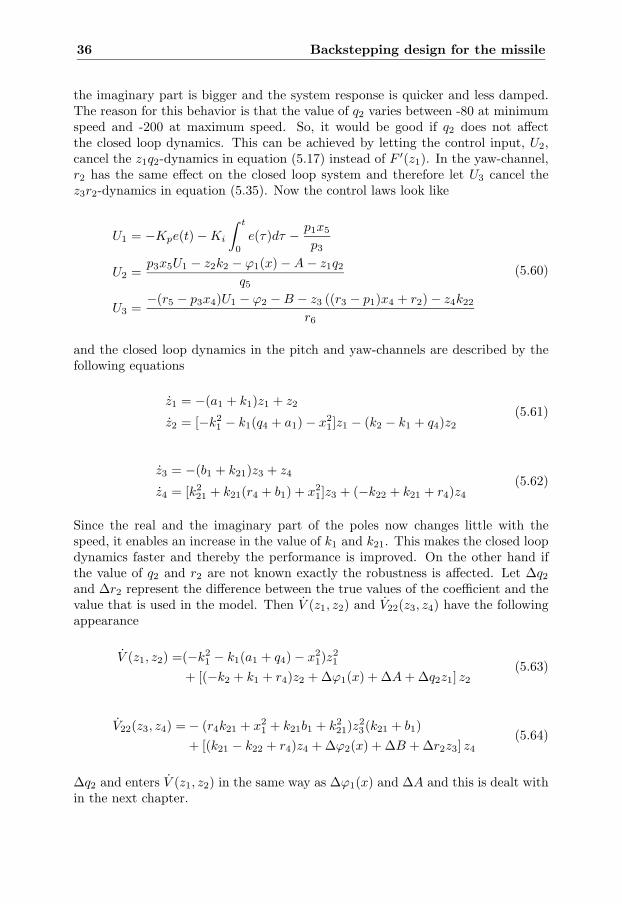
Since the real and the imaginary part of the poles now changes little with thespeed, it enables an increase in the value of k1 and k21. This makes the closed loopdynamics faster and thereby the performance is improved. On the other hand ifthe value of q2 and r2 are not known exactly the robustness is affected. Let ∆q2
and ∆r2 represent the difference between the true values of the coefficient and thevalue that is used in the model. Then V (z1, z2) and V22(z3, z4) have the followingappearance
V (z1, z2) =(−k21 − k1(a1 + q4) − x2
1)z21
+ [(−k2 + k1 + r4)z2 + ∆ϕ1(x) + ∆A + ∆q2z1] z2
(5.63)
V22(z3, z4) = − (r4k21 + x21 + k21b1 + k2
21)z23(k21 + b1)
+ [(k21 − k22 + r4)z4 + ∆ϕ2(x) + ∆B + ∆r2z3] z4
(5.64)
∆q2 and enters V (z1, z2) in the same way as ∆ϕ1(x) and ∆A and this is dealt within the next chapter.
5.4 Simulation 37
5.4 Simulation
5.4.1 Conditions
The following conditions are valid during the simulations.
• In the simulations the missile dynamics are calculated using the simulationmodel described in section 4.2.6, i.e. not the one that the design was builtupon.
• The aerodynamics coefficients are assumed to be known exactly. This meansthat the coefficients used in the control laws are the same as the coefficientswhich are used to calculate the dynamics of the missile.
• The initial speed of the missile is Mach 1.5 in simulation 5.1 and Mach 3.0in simulation 5.2.
• No noise or disturbances such as wind gusts are added.
• The sensors are ideal. The actuator dynamics are described in section 4.1.4and the fins have zero friction.
• In the controller, the derivatives of the reference signals are not used.
• The controller used in the simulations are the one that was derived in equation(5.60) in Section 5.3.4.
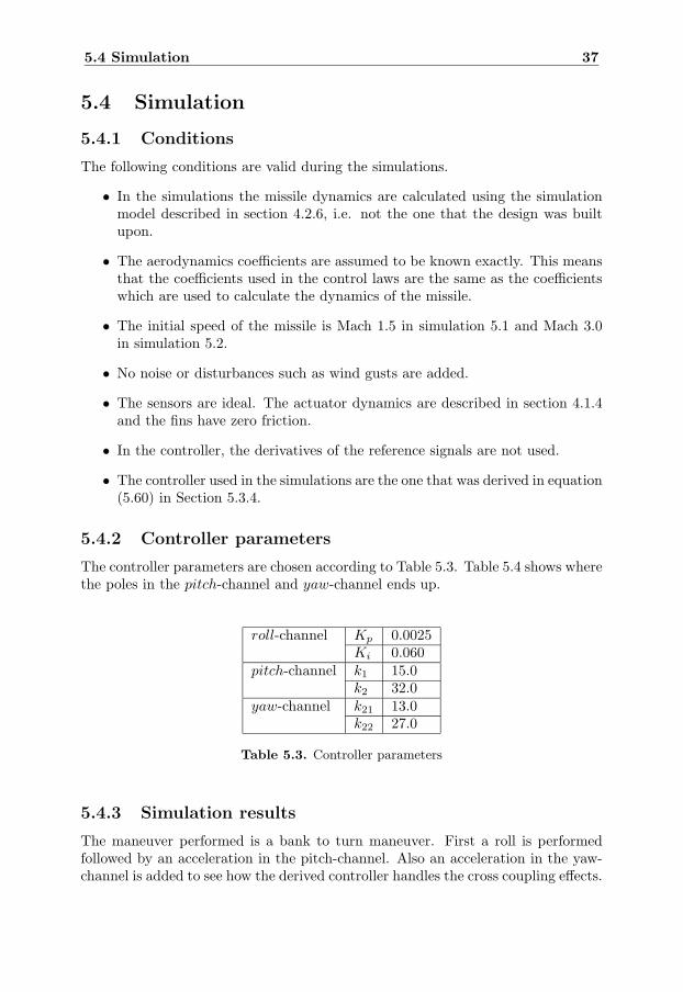
5.4.2 Controller parameters
The controller parameters are chosen according to Table 5.3. Table 5.4 shows wherethe poles in the pitch-channel and yaw-channel ends up.
roll-channel Kp 0.0025Ki 0.060
pitch-channel k1 15.0k2 32.0
yaw-channel k21 13.0k22 27.0
Table 5.3. Controller parameters
5.4.3 Simulation results
The maneuver performed is a bank to turn maneuver. First a roll is performedfollowed by an acceleration in the pitch-channel. Also an acceleration in the yaw-channel is added to see how the derived controller handles the cross coupling effects.
38 Backstepping design for the missile
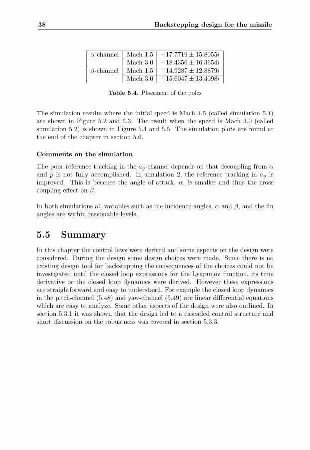
α-channel Mach 1.5 −17.7719 ± 15.8055iMach 3.0 −18.4356 ± 16.3654i
β-channel Mach 1.5 −14.9287 ± 12.8879iMach 3.0 −15.6047 ± 13.4098i
Table 5.4. Placement of the poles
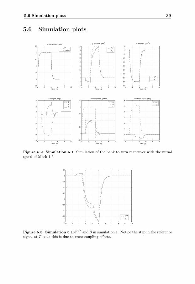
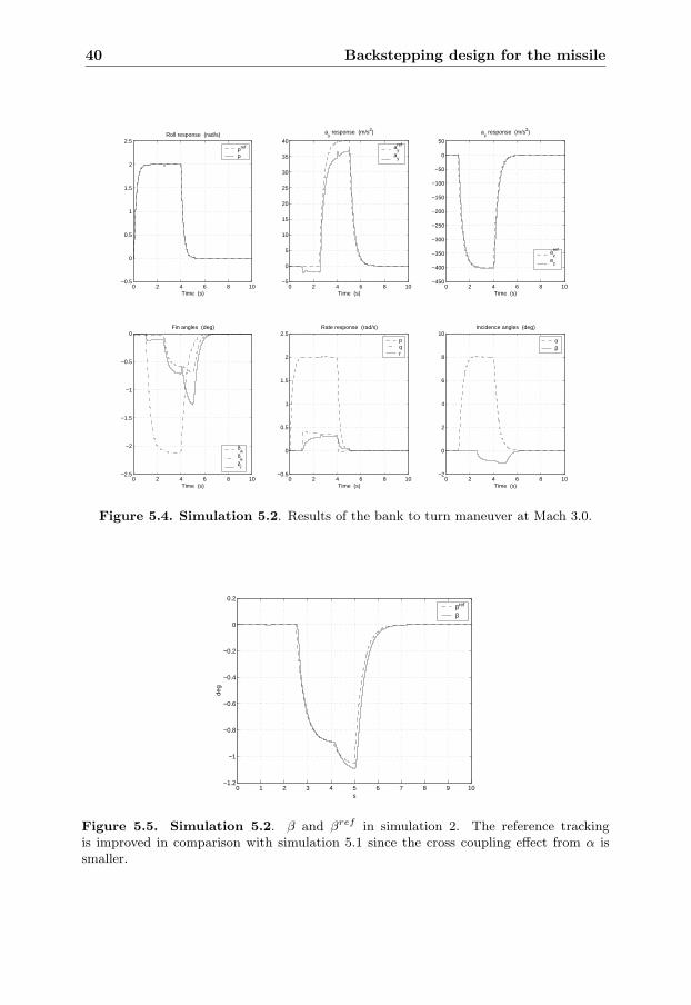
The simulation results where the initial speed is Mach 1.5 (called simulation 5.1)are shown in Figure 5.2 and 5.3. The result when the speed is Mach 3.0 (calledsimulation 5.2) is shown in Figure 5.4 and 5.5. The simulation plots are found atthe end of the chapter in section 5.6.
Comments on the simulation
The poor reference tracking in the ay-channel depends on that decoupling from αand p is not fully accomplished. In simulation 2, the reference tracking in ay isimproved. This is because the angle of attack, α, is smaller and thus the crosscoupling effect on β.
In both simulations all variables such as the incidence angles, α and β, and the finangles are within reasonable levels.
5.5 Summary
In this chapter the control laws were derived and some aspects on the design wereconsidered. During the design some design choices were made. Since there is noexisting design tool for backstepping the consequences of the choices could not beinvestigated until the closed loop expressions for the Lyapunov function, its timederivative or the closed loop dynamics were derived. However these expressionsare straightforward and easy to understand. For example the closed loop dynamicsin the pitch-channel (5.48) and yaw-channel (5.49) are linear differential equationswhich are easy to analyze. Some other aspects of the design were also outlined. Insection 5.3.1 it was shown that the design led to a cascaded control structure andshort discussion on the robustness was covered in section 5.3.3.
5.6 Simulation plots 39
5.6 Simulation plots
0 2 4 6 8 10−0.5
0
0.5
1
1.5
2
2.5
Time (s)
Roll response (rad/s)
pref
p (rad/s)
0 2 4 6 8 10−10
−5
0
5
10
15
20
25
30
35
40
Time (s)
ay response (m/s2)
ayref
ay
0 2 4 6 8 10−450
−400
−350
−300
−250
−200
−150
−100
−50
0
50
Time (s)
az response (m/s2)
azref
az
0 2 4 6 8 10−10
−8
−6
−4
−2
0
2
4
Time (s)
Fin angles (deg)
δa
δe
δr
0 2 4 6 8 10−0.5
0
0.5
1
1.5
2
2.5
Time (s)
Rate response (rad/s)
pqr
0 2 4 6 8 10−5
0
5
10
15
20
25
30
Time (s)
Incidence angles (deg)
αβ
Figure 5.2. Simulation 5.1. Simulation of the bank to turn maneuver with the initialspeed of Mach 1.5.
0 1 2 3 4 5 6 7 8 9 10−4
−3.5
−3
−2.5
−2
−1.5
−1
−0.5
0
0.5
βref
β
Figure 5.3. Simulation 5.1.βref and β in simulation 1. Notice the step in the referencesignal at T ≈ 4s this is due to cross coupling effects.
40 Backstepping design for the missile
0 2 4 6 8 10−0.5
0
0.5
1
1.5
2
2.5
Time (s)
Roll response (rad/s)
pref
p
0 2 4 6 8 10−5
0
5
10
15
20
25
30
35
40
Time (s)
ay response (m/s2)
ayref
ay
0 2 4 6 8 10−450
−400
−350
−300
−250
−200
−150
−100
−50
0
50
Time (s)
az response (m/s2)
azref
az
0 2 4 6 8 10−2.5
−2
−1.5
−1
−0.5
0
Time (s)
Fin angles (deg)
δa
δe
δr
0 2 4 6 8 10−0.5
0
0.5
1
1.5
2
2.5
Time (s)
Rate response (rad/s)
pqr
0 2 4 6 8 10−2
0
2
4
6
8
10
Time (s)
Incidence angles (deg)
αβ
Figure 5.4. Simulation 5.2. Results of the bank to turn maneuver at Mach 3.0.
0 1 2 3 4 5 6 7 8 9 10−1.2
−1
−0.8
−0.6
−0.4
−0.2
0
0.2
s
deg
βref
β
Figure 5.5. Simulation 5.2. β and βref in simulation 2. The reference trackingis improved in comparison with simulation 5.1 since the cross coupling effect from α issmaller.
Chapter 6
Dealing with uncertainties
All mathematical models of physical systems suffer from model errors and uncer-tainties. This means that the model which the control design is based on differsfrom the actual physical system. Despite that, the closed loop system must notonly be stable but it should also give good performance.
In the case of the missile, the aerodynamic coefficients are more or less uncertain.In section 5.3.3 an introduction to how these uncertainties affect the robustness ofthe closed loop system was given and some of the problems were illustrated. Herethe problems are explored further.
In the first section we return to the robustness discussion of section 5.3.3 andextend it. This will show that in the presence of uncertainties in the aerodynamiccoefficients, the closed looped system will reach an equilibrium point. However notthe one that was aimed for. In section 6.2, a method which will bring the systemto the desired equilibrium is therefore presented.
6.1 Extended robustness discussion
6.1.1 Problem review
In section 5.3.3 the problem of ensuring that the Lyapunov derivatives, V (z1, z2)and V22(z3, z4), are negative definite in the presence of uncertainties in the aerody-namic coefficients was presented. In equation (5.51) the unknown terms (sign andmagnitude) ∆ϕ1(x) and ∆A are a result of the uncertainties. In order to renderthat equation negative definite equation (5.52) must hold. Even if the size and signof ∆ϕ1(x) and ∆A are known, it is hard to find a combination of k1 and k2 suchthat equation (5.51) holds for all z2. Equation (5.63) corresponds to (5.51) but forthe controller which also cancels the q2-term.
41
42 Dealing with uncertainties
6.1.2 Using level curves for stability analysis
Equation (5.63) can be written on the following form
V (z1, z2) =(−k21 − k1(a1 + q4) − x2
1)z21
+ (−k2 + k1 + r4) z22 + (∆ϕ1(x) + ∆A)︸ ︷︷ ︸
∆Ez2
z2 + ∆q2︸︷︷︸∆Ez1z2
z1z2 (6.1)
∆Ez2 and ∆Ez1z2 are sometimes in this thesis referred to as error variables.
One realizes that the values of V (z1, z2) varies with the values of ∆Ez2 and ∆Ez1z2
but also with the values of z1 and z2. For example, if z1 = 0 and z2 = 0 thenV = 0. There are however, for some value of ∆Ez2 and ∆Ez1z2 , other values ofz1 and z2 which also corresponds to V = 0 and some who result in V > 0. Byviewing equation (6.1) as a function of two variables it is possible to make a plotof how V changes with z1 and z2(for some fixed ∆Ez2 and ∆Ez1z2). One way ofplotting this relationship is to plot the level curve where V = 0. Together with alevel curve plot for the Lyapunov function, V , a stability analysis can be done. Todo that the geometrical interpretation given in section 2.2.1 is extended to includethe case when V > 0. Here z1 is used instead of x and z2 instead of y.
When V (z1, z2) > 0 the angle θ is in the range [0, π/2]. This means that f(z1, z2)is pointing out from the origin and therefor the system moves away from it. Ifthe area where V (z1, z2) > 0 is closed, as shown in Figure 6.1, it means thattrajectories starting within that area will move towards the boundary of the areawhere V (z1, z2) = 0. Since outside this area the ideas developed in 2.2.1 are validand therefore the system will not continue to move into that zone and vice versa.This means that the system will find an equilibrium point on the circle whereV (z1, z2) = 0. If the area corresponding to V (z1, z2) > 0 is non closed area, a tra-jectory starting within the area may move away from the origin and since there areno boundary it can continue to move into infinity. Thus, the system can becomeunstable. See Figure 6.2.
Now, level curves for V (z1, z2) for different values of ∆Ez2 and ∆Ez1z2 are invest-igated. The discussion below is general and it is valid for both the yaw-channel,V22(z2, z4), and the pitch-channel, V (z1, z2). Note that it only considers the idealcase when there is movement in one channel at the time, i.e. the effects of crosscoupling are not considered. Further, to simplify the following discussion the errorvariables have fixed values, which is not always the case since they vary with time.
First, regard the case when there are no uncertainties. Then ∆Ez2 and ∆Ez1z2
equals zero. This corresponds to what we build our design on and not surprisinglythere is only one equilibrium point, namely the origin.
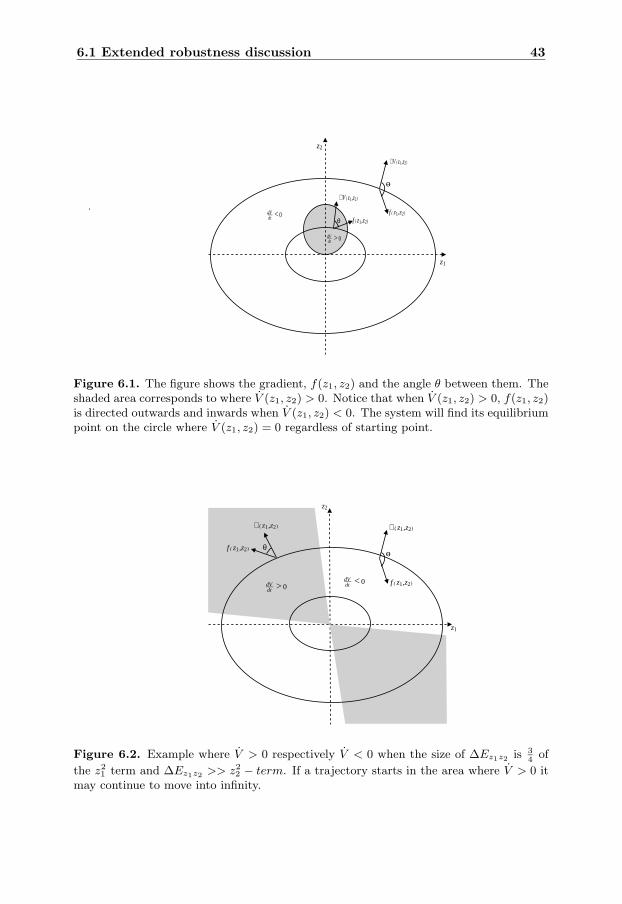
6.1 Extended robustness discussion 43
dVdt >0
dVdt <0−
f ( z1,z2)
f ( z1,z2)
∇ V ( z1,z2)
θ
θ
∇ V ( z1,z2)
z1
z2
Figure 6.1. The figure shows the gradient, f(z1, z2) and the angle θ between them. Theshaded area corresponds to where V (z1, z2) > 0. Notice that when V (z1, z2) > 0, f(z1, z2)is directed outwards and inwards when V (z1, z2) < 0. The system will find its equilibriumpoint on the circle where V (z1, z2) = 0 regardless of starting point.
θ
z1
z2
∇ ( z1,z2) ∇ ( z1,z2)
f ( z1,z2)
f ( z1,z2) θ
dVdt <0dV
dt >0
Figure 6.2. Example where V > 0 respectively V < 0 when the size of ∆Ez1z2 is 34
of
the z21 term and ∆Ez1z2 >> z2
2 − term. If a trajectory starts in the area where V > 0 itmay continue to move into infinity.
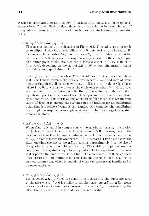
44 Dealing with uncertainties
When the error variables are non-zero a mathematical analysis of equation (6.1)shows where V > 0. Such analysis depends on the relation between the size ofthe quadratic terms and the error variables but some main features are presentedbelow.
• ∆Ez2 �= 0 and ∆Ez1z2 = 0:This case is similar to the situation in Figure 6.1. V equals zero on a circleor an ellipse. Inside that circle/ellipse V > 0, outside V < 0. The radius(R)increases with increasing ∆Ez2 (R → ∞ as ∆Ez2 → ∞). This means that thearea where V > 0 increases. The origin is always a point on the circle/ellipse.The center point of the circle/ellipse is located either in (0, z2 > 0) or in(0, z2 < 0), depending on the sign of ∆Ez2 . What does this mean in termsof stability and equilibrium points?
If the system is in the area where V > 0 it follows from the discussion abovethat it will move towards the circle/ellipse where V = 0 and stop at somepoint on that circle/ellipse or move along it. If it is outside the circle/ellipse,where V < 0, it will move towards the circle/ellipse where V = 0 and stopat some point on it or move along it. Hence, the system will always find anequilibrium point or move along the circle/ellipse and therefore it is stabilizedby the controller. This is true as long as the circle/ellipse radius is within somevalue. If R is large enough the system could be heading for an equilibriumpoint that is outside of what it can handle. For example, the equilibriumpoint might correspond to an angle of attack (α) that is so large that systembecomes unstable.
• ∆Ez2 = 0 and ∆Ez1z2 �= 0:When ∆Ez1z2 is small in comparison to the quadratic term z2
1 in equation(6.1), this has very little effect on the area where V > 0. The origin is still theonly point where V = 0. From a stability point of view this has no effect. As∆Ez1z2 becomes larger the area where V > 0 increases. Figure 6.2 shows thesituation when the size of the ∆Ez1z2-term is approximately 3
4 of the size ofthe quadratic z2
1 and much bigger than z22 . The stability properties are now
very poor. The system’s equilibrium point could lie anywhere on the linesthat separate the area where V < 0 from the area where V > 0. Since theselines stretch out into infinity this means that the system could be heading foran equilibrium point which is outside of what the system can handle, and itbecomes unstable.
• ∆Ez2 �= 0 and ∆Ez1z2 �= 0:For values of ∆Ez1z2 which are small in comparison to the quadratic termz21 the area where V > 0 is similar to the first case. As ∆Ez1z2 ∆Ez2 grows
the radius of the circle/ellipse increases and when ∆Ez1z2 becomes large theaffect that appeared in the second case becomes visible.
6.1 Extended robustness discussion 45
6.1.3 Identifying the ∆Ez2-terms and ∆Ez1z2-terms
In real situations, the ∆Ez2 -term and ∆Ez1z2-term are unknown. But it is possibleto write down an expression for them. By looking at which coefficients that makeup these expressions an understanding of how an error in some coefficient will af-fect the stability of the system can be obtained. If the errors are known, the valueof ∆Ez2 and ∆Ez1z2 can be calculated through the expressions. In simulationsthe error in some coefficient can be set to some known value and it is possible tokeep track of the ∆Ez2 -term and the ∆Ez1z2-term. So, at any time the stabilityproperties of the system can be examined. Below expressions for ∆Ez2 and ∆Ez1z2
in the pitch-channel are derived.(The procedure is equal in the yaw-channel but itis not presented, only the result.)
In section 5.2.1 the expression for V (z1, z2) was derived. Below it is given butthis time with the adjustments made in section 5.3.4.
V (z1, z2) = − (−k21 − k1(a1 + q4) − x2
1)(a1 + k1)z21
+ z2 [z2(q4 + k1) + ϕ1(x) + q2z1 + A + q5U2 − p3x5U1](6.2)
The control input U2 is chosen as
U2 =p3x5U1 − z2(k2 + k1) − ϕ1(x) − A + z1q2
q5(6.3)
where the ˆ represents the value of the coefficient that the model uses. Inserting(6.3) into (6.2) yields
V (z1, z2) =(−k21 − k1(a1 + q4) − x2
1)(a1 + k1)z21
+ z22(q4 − k2
q5q5
+ k1 − k1q5q5
)
+ [(ϕ1(x) − ϕ1(x)q5
q5) + (A − A
q5
q5) + (−p3x5U1 + p3x5U1
q5
q5)]
︸ ︷︷ ︸∆Ez2
z2
+ [(q2 − q2q5
q5)]
︸ ︷︷ ︸∆Ez1z2
z1z2
(6.4)
In equation (6.4) ∆Ez2 and ∆Ez1z2 can be identified and in section 5.2.1 theexpressions for ϕ1(x) and A are found,
ϕ1(x) =(q1 + 1)x1x3 + q3|x5| + (q4 + b1 − p2)x1x5 − x21α
ref − p1x25
A =(q2 + q4a1)αref(6.5)
Note that an error in q5 affects all the terms in equation (6.4) except for the firstone. If there are errors in the coefficients which are a part of ϕ1(x), then movement
46 Dealing with uncertainties
in another channel will contribute to ∆Ez2 and thus change the stability proper-ties. The size of ∆Ez2 is also affected by the size of the reference signal. In section5.3.4, U2 canceled the z1q2-dynamics to improve the performance of the closed loopsystem. There it was also mentioned that that choice might affect the robustness.Since q2 is a part of ∆Ez1z2 this choice has an effect on the robustness. It is im-portant to keep in mind that ∆Ez1z2 and ∆Ez2 may change during a maneuverwhich means that the stability properties are not static.
The corresponding expression to equation (6.4) in the yaw-channel is
V22(z3, z4) =
− (r2 + r4k21 + x21 + k21b1 + k2
21)z23(k21 + b1)
+ (k21 − k22 + r4)z24
+ [(ϕ2(x) − ϕ2(x)r6
r6) + (B − B
r6
r6) + ((r5 − p3x4)U1 − (r5 − p3x4)U1
r6
r6)]
︸ ︷︷ ︸∆Ez4
z4
+ [(r3 − p1 − (r3 − p1))r6
r6)x4 + (r2 − r2
r6
r6)]
︸ ︷︷ ︸∆Ez3z4
z3z4
(6.6)
6.1.4 Simulations
To show how to analyze the system’s stability properties by using level curves asimulation is presented, referred to as simulation 6.1. To avoid problems withconversion of the reference signal from affecting the results, the reference signal isgiven in α directly as a fixed value. This might seem strange, but what is of in-terest here is to show that the closed loop system will find an equilibrium point fora constant reference signal. A constant reference signal in the acceleration leads toa variable reference signal in α. This is because the coefficients that are used whentransforming the reference signal change during a maneuver, see equation (5.6).
The simulation is performed at a speed Mach 1.5 and initial altitude of 1000 m. AtT = 0s a step in α starts and is maintained throughout the rest of the simulation.To simulate errors in the coefficients, q5 and q2 is set to 0.8 and 1.2 times their realvalues respectively.
The step response in α is found in Figure 6.3. It shows a static error w.r.t. thedesired αref due to the error in q5 and q2. Figure 6.4 shows the level curves forV (z1, z2) and the z1 and z2 positions during the period 0.6-15 s. In the shaded areaV (z1, z2) > 0 at T = 4.6s and the “*” represent the (z1, z2) position at the samepoint in time. Since “*” lies on the circle where V = 0 the system is in equilibrium.
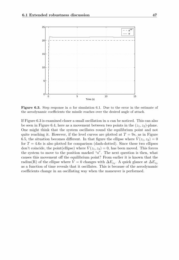
6.1 Extended robustness discussion 47
0 5 10 150
5
10
15
20
25
Time (s)
αref
α
Figure 6.3. Step response in α for simulation 6.1. Due to the error in the estimate ofthe aerodynamic coefficients the missile reaches over the desired angle of attack.
If Figure 6.3 is examined closer a small oscillation in α can be noticed. This can alsobe seen in Figure 6.4, here as a movement between two points in the (z1, z2)-plane.One might think that the system oscillates round the equilibrium point and notquite reaching it. However, if the level curves are plotted at T = 9s, as in Figure6.5, the situation becomes different. In that figure the ellipse where V (z1, z2) = 0for T = 4.6s is also plotted for comparison (dash-dotted). Since these two ellipsesdon’t coincide, the point(ellipse) where V (z1, z2) = 0, has been moved. This forcesthe system to move to the position marked “o”. The next question is then, whatcauses this movement off the equilibrium point? From earlier it is known that theradius(R) of the ellipse where V = 0 changes with ∆Ez2 . A quick glance at ∆Ez2
as a function of time reveals that it oscillates. This is because of the aerodynamiccoefficients change in an oscillating way when the maneuver is performed.
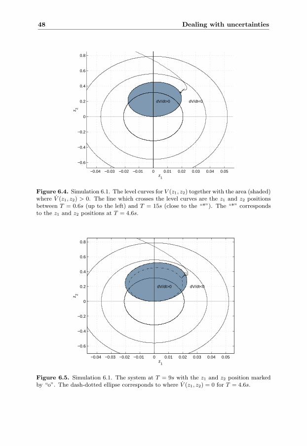
48 Dealing with uncertainties
−0.04 −0.03 −0.02 −0.01 0 0.01 0.02 0.03 0.04 0.05
−0.6
−0.4
−0.2
0
0.2
0.4
0.6
0.8
dV/dt<0dV/dt>0
z1
z 2
Figure 6.4. Simulation 6.1. The level curves for V (z1, z2) together with the area (shaded)where V (z1, z2) > 0. The line which crosses the level curves are the z1 and z2 positionsbetween T = 0.6s (up to the left) and T = 15s (close to the “*”). The “*” correspondsto the z1 and z2 positions at T = 4.6s.
−0.04 −0.03 −0.02 −0.01 0 0.01 0.02 0.03 0.04 0.05
−0.6
−0.4
−0.2
0
0.2
0.4
0.6
0.8
dV/dt<0dV/dt>0
z1
z 2
Figure 6.5. Simulation 6.1. The system at T = 9s with the z1 and z2 position markedby “o”. The dash-dotted ellipse corresponds to where V (z1, z2) = 0 for T = 4.6s.
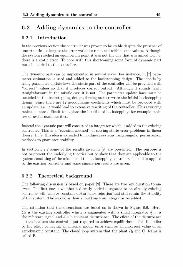
6.2 Adding dynamics to the controller 49
6.2 Adding dynamics to the controller
6.2.1 Introduction
In the previous section the controller was proven to be stable despite the presence ofuncertainties as long as the error variables remained within some values. Althoughthe system reached an equilibrium point it was not the one that was aimed for, i.e.there is a static error. To cope with this shortcoming some form of dynamic partmust be added to the controller.
The dynamic part can be implemented in several ways. For instance, in [7] para-meter estimation is used and added to the backstepping design. The idea is byusing parameter update laws the static part of the controller will be provided with“correct” values so that it produces correct output. Although it sounds fairlystraightforward in the missile case it is not. The parameter update laws must beincluded in the backstepping design, forcing us to rewrite the initial backsteppingdesign. Since there are 17 aerodynamic coefficients which must be provided withan update law, it would lead to extensive rewriting of the controller. This rewritingmakes it more difficult to explore the benefits of backstepping, for example makeuse of useful nonlinearities.
Instead the dynamic part will consist of an integrator which is added to the existingcontroller. This is a “classical method” of solving static error problems in lineartheory. In [9] this idea is extended to nonlinear systems using singular perturbationmethods to guarantee stability.
In section 6.2.2 some of the results given in [9] are presented. The purpose isnot to present the underlying theories but to show that they are applicable to thesystem consisting of the missile and the backstepping controller. Then it is appliedto the existing controller and some simulation results are given.
6.2.2 Theoretical background
The following discussion is based on paper [9]. There are two key question to an-swer. The first one is whether a directly added integrator to an already existingcontroller will achieve constant disturbance rejection and still retain the stabilityof the system. The second is, how should such an integrator be added.
The situation that the discussions are based on is shown in Figure 6.6. Here,C0 is the existing controller which is augmented with a small integrator ε
s , r isthe reference signal and d is a constant disturbance. The effect of the disturbanceis that it alters the control input required to achieve equilibrium. This is similarto the effect of having an internal model error such as an incorrect value of anaerodynamic constant. The closed loop system that the plant P0 and C0 forms iscalled P.
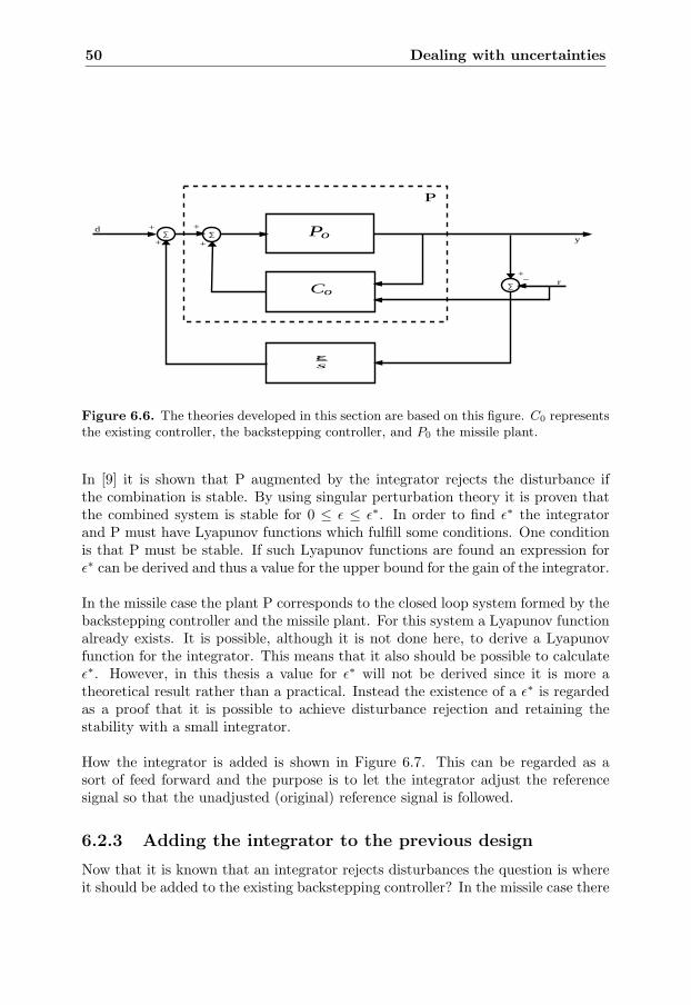
50 Dealing with uncertainties
y
r
d
P
+−
+
+
+
+∑ ∑
∑Co
Po
εs
Figure 6.6. The theories developed in this section are based on this figure. C0 representsthe existing controller, the backstepping controller, and P0 the missile plant.
In [9] it is shown that P augmented by the integrator rejects the disturbance ifthe combination is stable. By using singular perturbation theory it is proven thatthe combined system is stable for 0 ≤ ε ≤ ε∗. In order to find ε∗ the integratorand P must have Lyapunov functions which fulfill some conditions. One conditionis that P must be stable. If such Lyapunov functions are found an expression forε∗ can be derived and thus a value for the upper bound for the gain of the integrator.
In the missile case the plant P corresponds to the closed loop system formed by thebackstepping controller and the missile plant. For this system a Lyapunov functionalready exists. It is possible, although it is not done here, to derive a Lyapunovfunction for the integrator. This means that it also should be possible to calculateε∗. However, in this thesis a value for ε∗ will not be derived since it is more atheoretical result rather than a practical. Instead the existence of a ε∗ is regardedas a proof that it is possible to achieve disturbance rejection and retaining thestability with a small integrator.
How the integrator is added is shown in Figure 6.7. This can be regarded as asort of feed forward and the purpose is to let the integrator adjust the referencesignal so that the unadjusted (original) reference signal is followed.
6.2.3 Adding the integrator to the previous design
Now that it is known that an integrator rejects disturbances the question is whereit should be added to the existing backstepping controller? In the missile case there
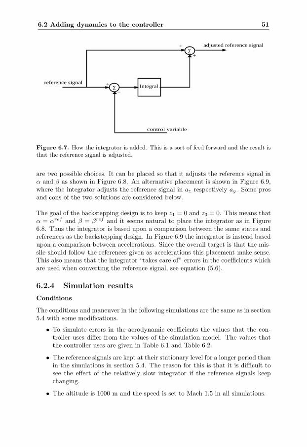
6.2 Adding dynamics to the controller 51
Integral
adjusted reference signal
reference signal +
−
+
+∑
∑
control variable
Figure 6.7. How the integrator is added. This is a sort of feed forward and the result isthat the reference signal is adjusted.
are two possible choices. It can be placed so that it adjusts the reference signal inα and β as shown in Figure 6.8. An alternative placement is shown in Figure 6.9,where the integrator adjusts the reference signal in az respectively ay. Some prosand cons of the two solutions are considered below.
The goal of the backstepping design is to keep z1 = 0 and z3 = 0. This means thatα = αref and β = βref and it seems natural to place the integrator as in Figure6.8. Thus the integrator is based upon a comparison between the same states andreferences as the backstepping design. In Figure 6.9 the integrator is instead basedupon a comparison between accelerations. Since the overall target is that the mis-sile should follow the references given as accelerations this placement make sense.This also means that the integrator “takes care of” errors in the coefficients whichare used when converting the reference signal, see equation (5.6).
6.2.4 Simulation results
Conditions
The conditions and maneuver in the following simulations are the same as in section5.4 with some modifications.
• To simulate errors in the aerodynamic coefficients the values that the con-troller uses differ from the values of the simulation model. The values thatthe controller uses are given in Table 6.1 and Table 6.2.
• The reference signals are kept at their stationary level for a longer period thanin the simulations in section 5.4. The reason for this is that it is difficult tosee the effect of the relatively slow integrator if the reference signals keepchanging.
• The altitude is 1000 m and the speed is set to Mach 1.5 in all simulations.
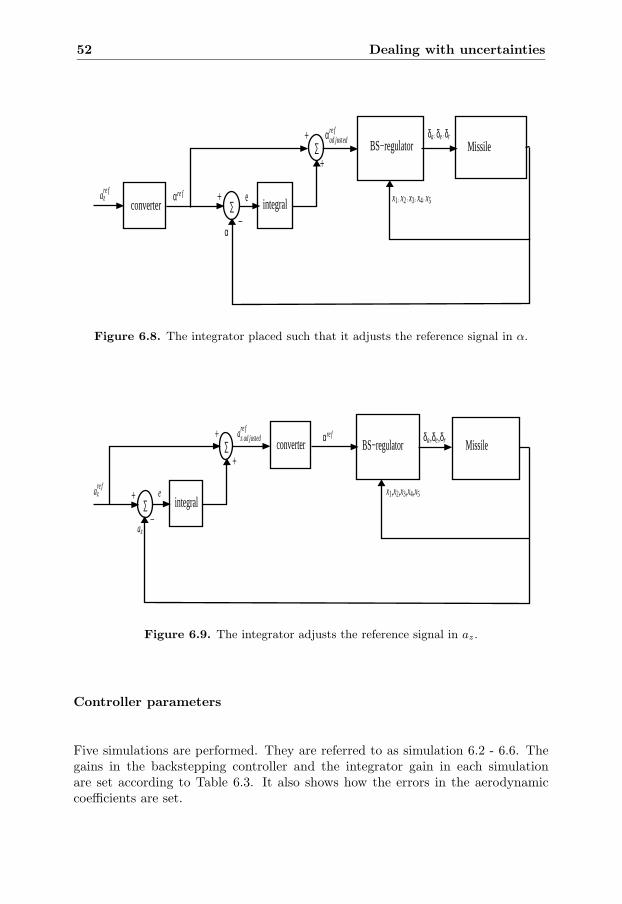
52 Dealing with uncertainties
MissileBS−regulator+
+
+
−converter
∑
∑ integralαre f
α
are fz
αre fad justed
x1; x2;x3;x4;x5
δa; δe;δr
e
Figure 6.8. The integrator placed such that it adjusts the reference signal in α.
MissileBS−regulator+
+
+
−
converter∑
∑ integralare f
z
αre f
az
are fz; ad justed δa,δe,δr
x1,x2,x3,x4,x5e
Figure 6.9. The integrator adjusts the reference signal in az.
Controller parameters
Five simulations are performed. They are referred to as simulation 6.2 - 6.6. Thegains in the backstepping controller and the integrator gain in each simulationare set according to Table 6.3. It also shows how the errors in the aerodynamiccoefficients are set.
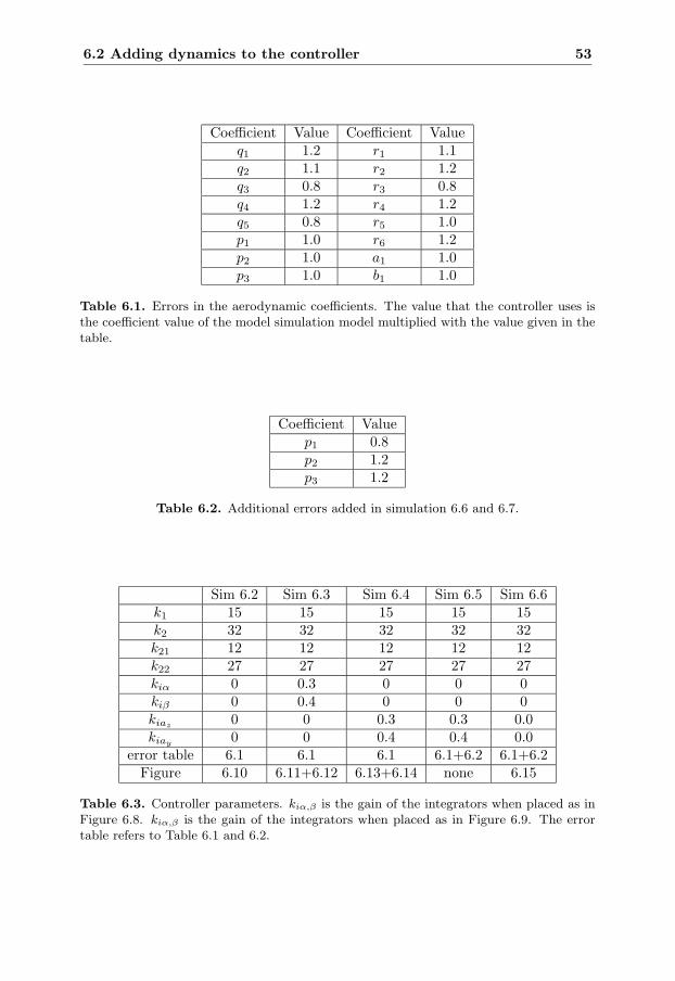
6.2 Adding dynamics to the controller 53
Coefficient Value Coefficient Valueq1 1.2 r1 1.1q2 1.1 r2 1.2q3 0.8 r3 0.8q4 1.2 r4 1.2q5 0.8 r5 1.0p1 1.0 r6 1.2p2 1.0 a1 1.0p3 1.0 b1 1.0
Table 6.1. Errors in the aerodynamic coefficients. The value that the controller uses isthe coefficient value of the model simulation model multiplied with the value given in thetable.
Coefficient Valuep1 0.8p2 1.2p3 1.2
Table 6.2. Additional errors added in simulation 6.6 and 6.7.
Sim 6.2 Sim 6.3 Sim 6.4 Sim 6.5 Sim 6.6k1 15 15 15 15 15k2 32 32 32 32 32k21 12 12 12 12 12k22 27 27 27 27 27kiα 0 0.3 0 0 0kiβ 0 0.4 0 0 0kiaz
0 0 0.3 0.3 0.0kiay
0 0 0.4 0.4 0.0error table 6.1 6.1 6.1 6.1+6.2 6.1+6.2
Figure 6.10 6.11+6.12 6.13+6.14 none 6.15
Table 6.3. Controller parameters. kiα,β is the gain of the integrators when placed as inFigure 6.8. kiα,β is the gain of the integrators when placed as in Figure 6.9. The errortable refers to Table 6.1 and 6.2.
54 Dealing with uncertainties
Comments on the simulations
The simulation plots are found in at the end of the chapter in section 6.5.
Simulation 6.2 In this simulation the integrators are not added for comparisonwith simulations with the integrators added. As seen in Figure 6.10 theequilibrium point in the yaw and pitch channels are moved, causing the missileto reach a greater acceleration than desired.
Simulation 6.3 Here the integrators are added so that they adjusts the referencesignals in α and β. As seen in Figure 6.11 the desired equilibrium point isnot reached since the integrators can not adjust for the errors that occurwhen converting the accelerations, az and ay into α and β. In Figure 6.12the adjusted reference signal and reference tracking in β is shown togetherwith the unadjusted reference signal.
Simulation 6.4 Simulation with the integrators added so that reference signalsin az and ay are adjusted. It illustrates that the desired equilibrium pointis reached because the integrators in this case also adjust for errors thatoccurs when converting the reference signals. Therefore this placement ofthe integrators is used in the forthcoming simulations.
Simulation 6.5 In this simulation the errors in the aerodynamic coefficients areset according to Table 6.1 and Table 6.2. Now the missile becomes unstable.
Simulation 6.6 This simulation is the same as in simulation 6.5 but the integ-rators are removed. The system is stable but the equilibrium point is veryfar from the desired. The side-slip angel, β, is large. Also oscillations occur.The overall performance is not acceptable.
In the simulations the integrator gain might seem quite large. The theories de-veloped in [9] considered that a small integrator is added. Since the missile becomesunstable in simulation 6.5 while it is still stable in simulation 6.6 one could cometo the conclusion that the integrator gain is too large. The results from simulation6.6 is however interesting in another way. It shows that the equilibrium point hasbeen moved so far away from the desired that the integrator is too slow to beable to bring the system back within a reasonable time. It is clear that there is aneed to compensate for the control error much faster. This can be achieved with aproportional part.
6.3 Increasing the gain in the backstepping loop
By looking at Figure 5.1 one notice that there is in fact already a proportional partimplemented in the backstepping control laws, namely k1 (k21 in the yaw-channel).So, by increasing k1 and k21 a faster compensation of the control error is achieved.On the other hand they can not be chosen arbitrary large. This has several reasons.Conditions (5.25) and (5.43) must hold. In section 5.3.2 it was shown that they
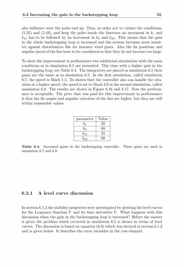
6.3 Increasing the gain in the backstepping loop 55
also influence were the poles end up. Thus, in order not to violate the conditions,(5.25) and (5.43), and keep the poles inside the bisectors an increment in k1 andk21 has to be followed by an increment in k2 and k22. This means that the gainin the whole backstepping loop is increased and the system becomes more sensit-ive against disturbances like for instance wind gusts. Also the fin positions andangular speed of the fins have to be considered so that they do not become too large.
To show the improvement in performance two additional simulations with the sameconditions as in simulation 6.5 are presented. This time with a higher gain in thebackstepping loop, see Table 6.4. The integrators are placed as simulation 6.5 theirgains are the same as in simulation 6.5. In the first simulation, called simulation6.7, the speed is Mach 1.5. To shown that the controller also can handle the situ-ation at a higher speed, the speed is set to Mach 3.0 in the second simulation, calledsimulation 6.8. The results are shown in Figure 6.16 and 6.17. Now the perform-ance is acceptable. The price that was paid for this improvement in performanceis that the fin angles and angular velocities of the fins are higher, but they are stillwithin reasonable values.
parameter Valuek1 35k2 68k21 35k22 68
Table 6.4. Increased gains in the backstepping controller. These gains are used insimulation 6.7 and 6.8.
6.3.1 A level curve discussion
In section 6.1.2 the stability properties were investigated by plotting the level curvesfor the Lyapunov function V and its time derivative V . What happens with thisdiscussion when the gain in the backstepping loop is increased? Before the answeris given the problem which occurred in simulation 6.5 is shown in terms of levelcurves. The discussion is based on equation (6.6) which was derived in section 6.1.2and is given below. It describes the error variables in the yaw-channel.
56 Dealing with uncertainties
V22(z3, z4) =
− (r2 + r4k21 + x21 + k21b1 + k2
21)z23(k21 + b1)
+ (k21 − k22 + r4)z24
+ [(ϕ2(x) − ϕ2(x)r6
r6) + (B − B
r6
r6) + ((r5 − p3x4)U1 − (r5 − p3x4)U1
r6
r6)]
︸ ︷︷ ︸∆Ez4
z4
+ [(r3 − p1 − (r3 − p1)r6
r6)x4 + (r2 − r2
r6
r6)]
︸ ︷︷ ︸∆Ez3z4
z3z4
(6.7)
In simulation 6.2, ∆Ez3z4 = −300 and ∆Ez4 = 5, but in simulation 6.5 ∆Ez3z4 =−300 and ∆Ez4 = 25. Since the radius of the circle/ellipse where V = 0 increaseswhen ∆Ez4 increases this explains why the equilibrium point is so far from thedesirable.
From (6.7) it is clear that increasing k21 and k22 only affects the z23-term and
the z24-term while the error variables are left unchanged. Hereby the relation in
size between the z23-term and the z2
4-term and the error variables is changed. Theoverall effect is that the area where V22(z3, z4) > 0 is decreased and the equilibriumpoint will be closer to the desirable.
6.4 Summary
This chapter has focused on how the uncertainties in the aerodynamic coefficientsaffected the closed loop system, i.e the robustness. This was investigated by plot-ting the Lyapunov function and its time derivative as level curves. Based on thesize and appearance of the area where V > 0 the stability properties were outlined.Since this area is very crucial it was shown how it varied with the size of the socalled error variables. An algebraic expression for the error variables were also de-rived in equation (6.4) and equation (6.6). Trough these expressions it is possibleto analyze how an error in the aerodynamic coefficients affects the error variablesand thus the stability properties of the closed loop.
The closed loop system reached, in most cases, an equilibrium point despite er-ror in the aerodynamic coefficients. However not the desired one. To bring thesystem to the desired equilibrium point dynamics was added to the controller inform of an integrator. The integrator adjusts the reference signal so that the desiredoutput is achieved. By the theories developed in [9] it was shown that if the gainof the integrator is chosen properly it does not affect the stability. The reason thatan integrator was chosen instead of for example parameter update laws is that thelatter would have lead to an extensive rewriting of the already designed controller.
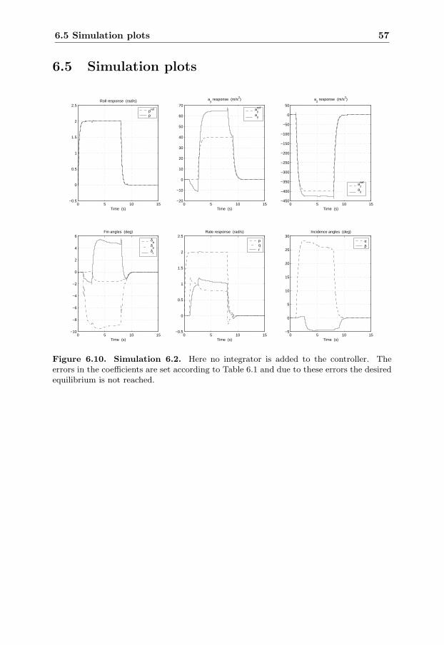
6.5 Simulation plots 57
6.5 Simulation plots
0 5 10 15−0.5
0
0.5
1
1.5
2
2.5
Time (s)
Roll response (rad/s)
pref
p
0 5 10 15−20
−10
0
10
20
30
40
50
60
70
Time (s)
ay response (m/s2)
ayref
ay
0 5 10 15−450
−400
−350
−300
−250
−200
−150
−100
−50
0
50
Time (s)
az response (m/s2)
azref
az
0 5 10 15−10
−8
−6
−4
−2
0
2
4
6
Time (s)
Fin angles (deg)
δa
δe
δr
0 5 10 15−0.5
0
0.5
1
1.5
2
2.5
Time (s)
Rate response (rad/s)
pqr
0 5 10 15−5
0
5
10
15
20
25
30
Time (s)
Incidence angles (deg)
αβ
Figure 6.10. Simulation 6.2. Here no integrator is added to the controller. Theerrors in the coefficients are set according to Table 6.1 and due to these errors the desiredequilibrium is not reached.
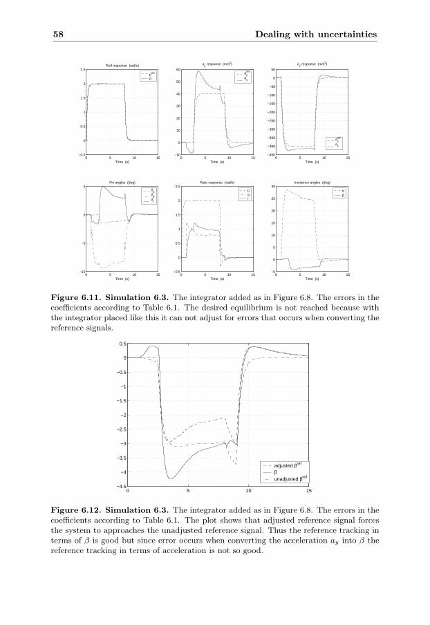
58 Dealing with uncertainties
0 5 10 15−0.5
0
0.5
1
1.5
2
2.5
Time (s)
Roll response (rad/s)
pref
p
0 5 10 15−10
0
10
20
30
40
50
60
Time (s)
ay response (m/s2)
ayref
ay
0 5 10 15−450
−400
−350
−300
−250
−200
−150
−100
−50
0
50
Time (s)
az response (m/s2)
azref
az
0 5 10 15−10
−5
0
5
Time (s)
Fin angles (deg)
δa
δe
δr
0 5 10 15−0.5
0
0.5
1
1.5
2
2.5
Time (s)
Rate response (rad/s)
pqr
0 5 10 15−5
0
5
10
15
20
25
30
Time (s)
Incidence angles (deg)
αβ
Figure 6.11. Simulation 6.3. The integrator added as in Figure 6.8. The errors in thecoefficients according to Table 6.1. The desired equilibrium is not reached because withthe integrator placed like this it can not adjust for errors that occurs when converting thereference signals.
0 5 10 15−4.5
−4
−3.5
−3
−2.5
−2
−1.5
−1
−0.5
0
0.5
adjusted βref
βunadjusted βref
Figure 6.12. Simulation 6.3. The integrator added as in Figure 6.8. The errors in thecoefficients according to Table 6.1. The plot shows that adjusted reference signal forcesthe system to approaches the unadjusted reference signal. Thus the reference tracking interms of β is good but since error occurs when converting the acceleration ay into β thereference tracking in terms of acceleration is not so good.
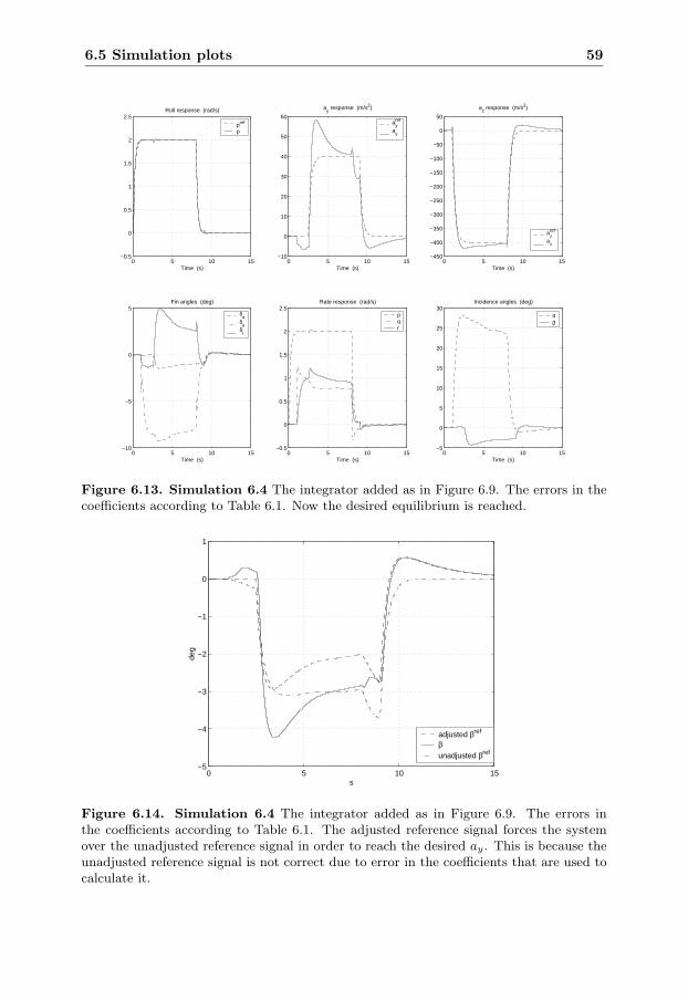
6.5 Simulation plots 59
0 5 10 15−0.5
0
0.5
1
1.5
2
2.5
Time (s)
Roll response (rad/s)
pref
p
0 5 10 15−10
0
10
20
30
40
50
60
Time (s)
ay response (m/s2)
ayref
ay
0 5 10 15−450
−400
−350
−300
−250
−200
−150
−100
−50
0
50
Time (s)
az response (m/s2)
azref
az
0 5 10 15−10
−5
0
5
Time (s)
Fin angles (deg)
δa
δe
δr
0 5 10 15−0.5
0
0.5
1
1.5
2
2.5
Time (s)
Rate response (rad/s)
pqr
0 5 10 15−5
0
5
10
15
20
25
30
Time (s)
Incidence angles (deg)
αβ
Figure 6.13. Simulation 6.4 The integrator added as in Figure 6.9. The errors in thecoefficients according to Table 6.1. Now the desired equilibrium is reached.
0 5 10 15−5
−4
−3
−2
−1
0
1
s
deg
adjusted βref
βunadjusted βref
Figure 6.14. Simulation 6.4 The integrator added as in Figure 6.9. The errors inthe coefficients according to Table 6.1. The adjusted reference signal forces the systemover the unadjusted reference signal in order to reach the desired ay. This is because theunadjusted reference signal is not correct due to error in the coefficients that are used tocalculate it.
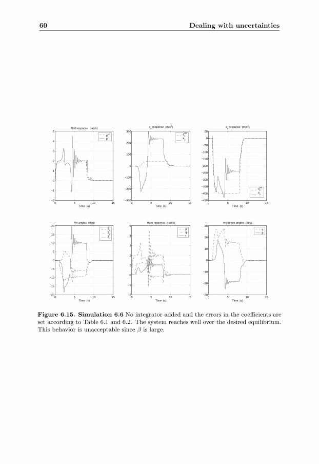
60 Dealing with uncertainties
0 5 10 15−2
−1
0
1
2
3
4
5
Time (s)
Roll response (rad/s)
pref
p
0 5 10 15−300
−200
−100
0
100
200
300
Time (s)
ay response (m/s2)
ayref
ay
0 5 10 15−450
−400
−350
−300
−250
−200
−150
−100
−50
0
50
Time (s)
az response (m/s2)
azref
az
0 5 10 15−20
−15
−10
−5
0
5
10
15
20
Time (s)
Fin angles (deg)
δa
δe
δr
0 5 10 15−2
−1
0
1
2
3
4
5
Time (s)
Rate response (rad/s)
pqr
0 5 10 15−30
−20
−10
0
10
20
30
Time (s)
Incidence angles (deg)
αβ
Figure 6.15. Simulation 6.6 No integrator added and the errors in the coefficients areset according to Table 6.1 and 6.2. The system reaches well over the desired equilibrium.This behavior is unacceptable since β is large.
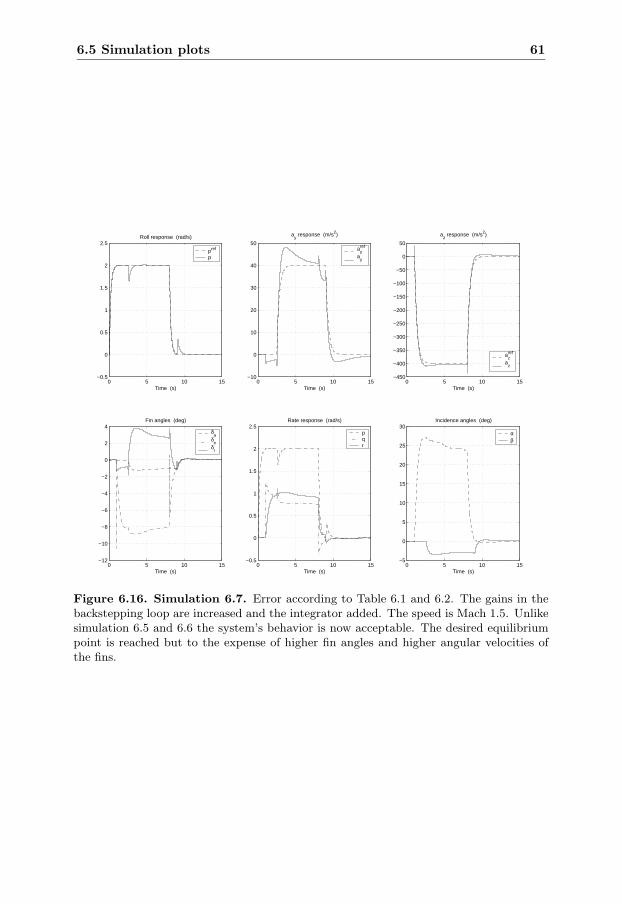
6.5 Simulation plots 61
0 5 10 15−0.5
0
0.5
1
1.5
2
2.5
Time (s)
Roll response (rad/s)
pref
p
0 5 10 15−10
0
10
20
30
40
50
Time (s)
ay response (m/s2)
ayref
ay
0 5 10 15−450
−400
−350
−300
−250
−200
−150
−100
−50
0
50
Time (s)
az response (m/s2)
azref
az
0 5 10 15−12
−10
−8
−6
−4
−2
0
2
4
Time (s)
Fin angles (deg)
δa
δe
δr
0 5 10 15−0.5
0
0.5
1
1.5
2
2.5
Time (s)
Rate response (rad/s)
pqr
0 5 10 15−5
0
5
10
15
20
25
30
Time (s)
Incidence angles (deg)
αβ
Figure 6.16. Simulation 6.7. Error according to Table 6.1 and 6.2. The gains in thebackstepping loop are increased and the integrator added. The speed is Mach 1.5. Unlikesimulation 6.5 and 6.6 the system’s behavior is now acceptable. The desired equilibriumpoint is reached but to the expense of higher fin angles and higher angular velocities ofthe fins.
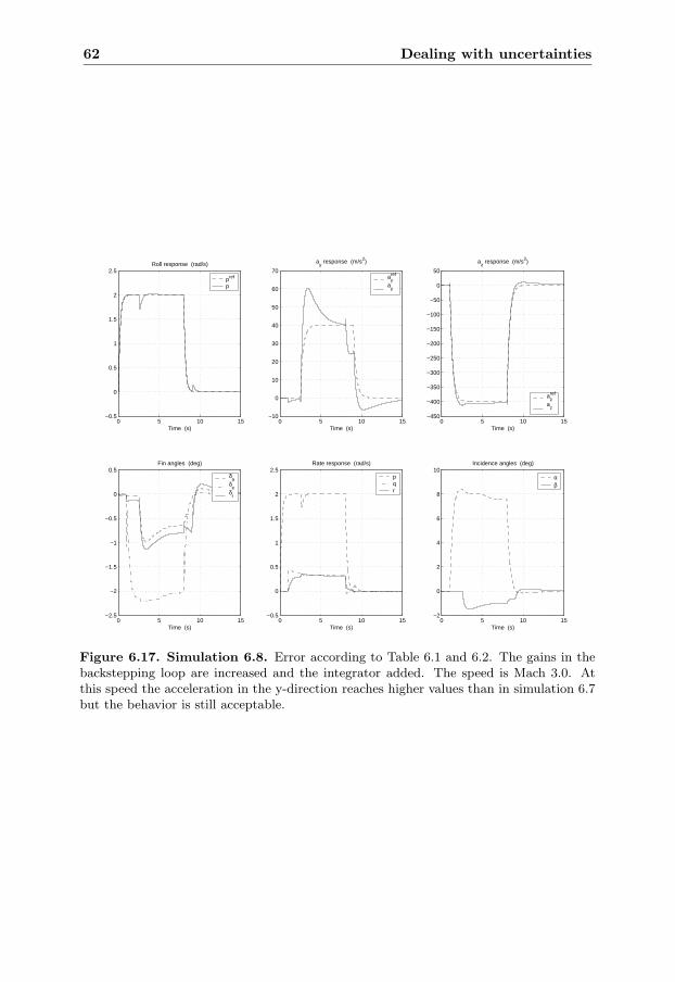
62 Dealing with uncertainties
0 5 10 15−0.5
0
0.5
1
1.5
2
2.5
Time (s)
Roll response (rad/s)
pref
p
0 5 10 15−10
0
10
20
30
40
50
60
70
Time (s)
ay response (m/s2)
ayref
ay
0 5 10 15−450
−400
−350
−300
−250
−200
−150
−100
−50
0
50
Time (s)
az response (m/s2)
azref
az
0 5 10 15−2.5
−2
−1.5
−1
−0.5
0
0.5
Time (s)
Fin angles (deg)
δa
δe
δr
0 5 10 15−0.5
0
0.5
1
1.5
2
2.5
Time (s)
Rate response (rad/s)
pqr
0 5 10 15−2
0
2
4
6
8
10
Time (s)
Incidence angles (deg)
αβ
Figure 6.17. Simulation 6.8. Error according to Table 6.1 and 6.2. The gains in thebackstepping loop are increased and the integrator added. The speed is Mach 3.0. Atthis speed the acceleration in the y-direction reaches higher values than in simulation 6.7but the behavior is still acceptable.
Chapter 7
Conclusions and future work
7.1 Conclusions
Stated below is a compilation of the most important results reached in this thesis.
The derived control laws led to that the closed loop dynamics can be expressedas linear differential equations. These are easy to deal with and linear theory canbe used to analyze the closed loop system.
The consequences of a certain design choice can be hard to determine before ex-pressions for the closed loop system has been derived.
Uncertainties in the aerodynamic coefficients affect the closed loop system, i.e.the robustness. It is possible to derive an algebraic expression which will tell howan error in the estimate of certain aerodynamic coefficient affects the stability prop-erties of the closed loop system.
In most cases the missile reaches an equilibrium point despite errors in the aerody-namic coefficients, but not necessarily the one that is aimed for for. By introducinga small integrator the desired equilibrium point can be reached with retained sta-bility.
7.2 Future work
In this thesis various design choices have been taken into consideration but thereexists others. Therefore, a designer who is more experienced in missile dynamicsmight come up with a design which differs a lot from the one that has been derivedin this thesis. It can therefore be interesting to look at how other design choicesaffect the closed loop dynamics and robustness. The idea of using level curves anderror variables can still be used. Another issue worth considering is to examine
63
64 Conclusions and future work
further how the size of the error variables affects the area where V > 0. Such ananalysis could also include an examination of the expression that make up the errorvariables. It could lead to a better understanding of in which aerodynamic coeffi-cients an error has the greatest effect on the robustness. Perhaps these variablesthen can be provided with a parameter update law.
In this thesis the sensitivity of the design has not been considered at all. Ofcourse this has to be taken into account if the design is to be implemented. Also,when adding an integrator it is wise to implement some sort of anti-windup, thishas not been considered.
Bibliography
[1] W.E. Boyce and R.C. DiPrima. Elementary differential equations and bound-ary value problems. John Wiely and Sons, United States Of America, 6thedition, 1997.
[2] T. Glad and L. Ljung. Reglerteknik. Grundlaggande teori. Studentlitteratur,Lund, Sweden, 2nd edition, 1989. In Swedish.
[3] T. Glad and L. Ljung. Reglerteori. Flervariabla och olinjara metoder. Stu-dentlitteratur, Lund, Sweden, 1994.
[4] O. Harkegard. Flight control design using Backstepping. Licentiate thesis875, Department of Electrical Engineering, Linkoping University, Linkoping,Sweden, May 1990.
[5] H. Jonson. Rtf. olinjara regulatorer. etapp 5. Technical Report RD-R00:6200F,Saab Dynamics, Saab Dynamics, Linkoping, Sweden, 1999.
[6] K. Karling. Aerodynamiska grundbegrepp. Kompendium och handbok. Arkitek-tkopia, Linkoping, Sweden, 12th edition, 1999.
[7] M. Krstic, I. Kanellakopoulos, and P. Kokotovic. Nonlinear and adaptivecontrol design. John Wiely and Sons, United States Of America, 1995.
[8] J.L. Meriam and L.G. Kraige. Engineering Mechanics. Dynamics. John Wielyand Sons, United States Of America, 4th edition, 1998.
[9] Brian D. O. Anderson Steven W. Su and Thomas S. Brinsmead. Constant dis-turbance suppression for nonlinear systems design using singular perturbationtheory. In Proceedings of the 40th IEEE Conferance on Decision and Control,pages 3272–3277, Orlando,Florida USA, December 2001.
[10] E. Wanstrom. Styrning och analys av olinjar robot med hjalp av backstep-ping. Master’s thesis LiTH-ISY-EX-3166, Department of Electrical Engineer-ing, Linkoping University, Linkoping, Sweden, October 2001.
65

66 Conclusions and future work
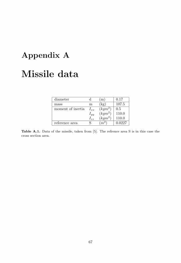
Appendix A
Missile data
diameter d (m) 0.17mass m (kg) 107.5moment of inertia Ixx (kgm2) 0.5
Iyy (kgm2) 110.0Izz (kgm2) 110.0
reference area S (m2) 0.0227
Table A.1. Data of the missile, taken from [5]. The refrence area S is in this case thecross section area.
67

68 Missile data
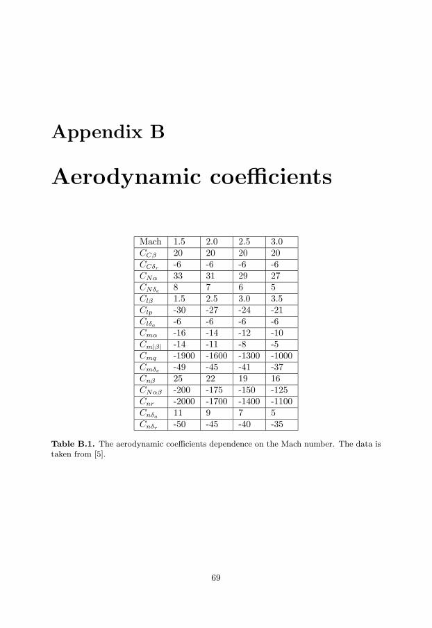
Appendix B
Aerodynamic coefficients
Mach 1.5 2.0 2.5 3.0CCβ 20 20 20 20CCδr
-6 -6 -6 -6CNα 33 31 29 27CNδe
8 7 6 5Clβ 1.5 2.5 3.0 3.5Clp -30 -27 -24 -21Clδa
-6 -6 -6 -6Cmα -16 -14 -12 -10Cm|β| -14 -11 -8 -5Cmq -1900 -1600 -1300 -1000Cmδe
-49 -45 -41 -37Cnβ 25 22 19 16CNαβ -200 -175 -150 -125Cnr -2000 -1700 -1400 -1100Cnδa
11 9 7 5Cnδr
-50 -45 -40 -35
Table B.1. The aerodynamic coefficients dependence on the Mach number. The data istaken from [5].
69
På svenska
Detta dokument hålls tillgängligt på Internet – eller dess framtida ersättare –under en längre tid från publiceringsdatum under förutsättning att inga extra-ordinära omständigheter uppstår.
Tillgång till dokumentet innebär tillstånd för var och en att läsa, ladda ner,skriva ut enstaka kopior för enskilt bruk och att använda det oförändrat för ick-ekommersiell forskning och för undervisning. Överföring av upphovsrätten viden senare tidpunkt kan inte upphäva detta tillstånd. All annan användning avdokumentet kräver upphovsmannens medgivande. För att garantera äktheten,säkerheten och tillgängligheten finns det lösningar av teknisk och administrativart.Upphovsmannens ideella rätt innefattar rätt att bli nämnd som upphovsman i denomfattning som god sed kräver vid användning av dokumentet på ovan beskrivnasätt samt skydd mot att dokumentet ändras eller presenteras i sådan form eller isådant sammanhang som är kränkande för upphovsmannens litterära eller konst-närliga anseende eller egenart.
För ytterligare information om Linköping University Electronic Press se för-lagets hemsidahttp://www.ep.liu.se/
In English
The publishers will keep this document online on the Internet - or its possiblereplacement - for a considerable time from the date of publication barring excep-tional circumstances.
The online availability of the document implies a permanent permission foranyone to read, to download, to print out single copies for your own use and touse it unchanged for any non-commercial research and educational purpose. Sub-sequent transfers of copyright cannot revoke this permission. All other uses ofthe document are conditional on the consent of the copyright owner. The pub-lisher has taken technical and administrative measures to assure authenticity,security and accessibility.
According to intellectual property law the author has the right to be men-tioned when his/her work is accessed as described above and to be protectedagainst infringement.
For additional information about the Linköping University Electronic Pressand its procedures for publication and for assurance of document integrity, pleaserefer to its WWW home page:http://www.ep.liu.se/
© Johan Dahlgren


![Robust H Autopilot Design for Agile Missile With …batti/progetti_fda/47.pdfII. MISSILE MODELING A. Nonlinear Model In this paper, the AIM-9X missile [18] equipped with a thrust vectoring](https://img.pdfslide.us/doc/110x75/5e8e2fd0378fff744940f04c/robust-h-autopilot-design-for-agile-missile-with-battiprogettifda47pdf-ii-missile.jpg)