Robust Multi-Period Vehicle Routing under Customer Order

Uncertainty

Anirudh Subramanyam1, Frank Mufalli2, Jose M. Laınez-Aguirre2, Jose M. Pinto3, and

Chrysanthos E. Gounaris∗1

1Department of Chemical Engineering, Carnegie Mellon University, Pittsburgh, PA, USA

2Praxair Inc., Tonawanda, NY, USA

3Praxair Inc., Danbury, CT, USA

Abstract

In this paper, we study multi-period vehicle routing problems where the aim is to determine

a minimum cost visit schedule and associated routing plan for each period using capacity-

constrained vehicles. In our setting, we allow for customer service requests that are received

dynamically over the planning horizon. In order to guarantee the generation of routing plans

that can flexibly accommodate potential service requests that have not yet been placed, we

model future potential service requests as binary random variables, and we seek to determine a

visit schedule that remains feasible for all anticipated realizations of service requests. To that

end, the decision-making process can be viewed as a multi-stage robust optimization problem

with binary recourse decisions. We approximate the multi-stage problem via a non-anticipative

two-stage model for which we propose a novel integer programming formulation and a branch-

and-cut solution approach. In order to investigate the quality of the solutions we obtain, we

also derive a valid lower bound on the multi-stage problem and present numerical schemes for

its computation. Computational experiments on benchmark datasets show that our approach

is practically tractable and generates high quality robust plans that significantly outperform

existing approaches in terms of both operational costs and fleet utilization.

∗Corresponding author: gounaris@cmu.edu

1

1 Introduction

The Vehicle Routing Problem (VRP) pertains to the design of cost-optimal routes for a fleet of

vehicles so as to serve a set of geographically dispersed customers. It is central to the field of

supply chain management and has been studied for over sixty years. The VRP has applications

in a wide variety of enterprises including manufacturing and retail distribution, waste collection,

postal services and transportation network design, to name but a few. We refer the reader to the

texts by Golden et al. [2008] and Toth and Vigo [2014] for an overview of the VRP and its variants.

Traditional variants of the VRP are of an operational nature and the typical setting involves

routing within a single period, e.g., a work day. However, several transportation problems arising

in practice are of a tactical nature, since they involve the routing of vehicles over multiple service

periods, e.g., a week. This is particularly the case when customers may dynamically place service

requests on any given day of the week, and each request specifies a set of future days during which

service can take place. At the end of each day, the distributor must make scheduling decisions to

assign a visit day to each unfulfilled service request, along with the standard routing decisions, so as

to minimize the long-term transportation costs. The tactical plan is implemented in a rolling horizon

fashion: only routes of the first day are executed while new service requests are received; unfulfilled

requests at the end of the first day and new requests accumulated during the day constitute the

new portfolio of orders to be considered for scheduling the following day. Such decision-making

setups are typical in systems in which services are provided by appointment, and the following

section describes one such system.

1.1 Industrial Motivation

Our research is motivated by the business setting of Praxair, Inc., an industrial gases company.

Praxair’s main production process involves separating air into its components, primarily nitrogen,

oxygen and argon, which are then used for a wide variety of industrial, medical, retail and other

purposes. After production, these gases are filled in cylinders that are to be transported to the

customers using trucks. Distribution operations involve receiving orders from customers during

the day. In addition to the order volume, customers in certain markets specify earliest and latest

acceptable visit dates at the time of placing their order. The resulting “day windows” are allowed

to be open, so that the distributor does not need to commit to a delivery date at the time of order

2

placement. Therefore, on any given day of operation, the goal is to decide which unfulfilled orders

to serve and which ones to leave for future days. The delivery schedules themselves are generated

by solving a traditional VRP, considering constraints on the number of trucks, their capacity, as

well as driver availability.

During this decision-making process, it is crucial to anticipate future customer orders and

explicitly hedge against their underlying uncertainty. Indeed, ignoring the possibility that customers

will place orders in the future can lead to infeasible situations, e.g., the number of vehicles required

may be more than what is available. This situation could arise because too many orders were

postponed until their latest acceptable dates, and huge costs must now be incurred to recover

feasible schedules (e.g., additional vehicles must be commissioned or drivers must be paid overtime).

The alternative is to serve orders beyond their acceptable dates; however, this is typically avoided,

since it is perceived as poor customer service and has a negative impact on the company’s reputation.

The above description of the VRP is representative of the problem and its complexities at

other companies as well as industries. Relevant examples include scheduling of maintenance per-

sonnel [Bostel et al., 2008, Tang et al., 2007, Tricoire, 2007], blood delivery to hospitals [Andreatta

and Lulli, 2008, Hemmelmayr et al., 2009], food distribution and collection [Wen et al., 2010,

Dayarian et al., 2015], courier services [Athanasopoulos and Minis, 2011], auto-carrier transporta-

tion [Cordeau et al., 2015], as well as distribution operations arising in city logistics [Archetti et al.,

2015]. Fortunately, companies that are faced with such operations often have significant amounts

of historical data, which can be used to obtain demand forecasts and provide information regarding

calls for service in future time periods. The objective of this paper is to contribute a decision sup-

port methodology that can use this information and generate risk-averse schedules for the tactical

planning of multi-period vehicle routing operations.

1.2 Related Work

A tactical level multi-period routing problem was first introduced by Angelelli et al. [2007a,b], who

considered the problem in which a number of customer requests are received at the beginning of

each day, and each of these requests must be served using a single uncapacitated vehicle either in the

day it was received or in the following day. The decision-maker must thus decide at the beginning

of each day which unfulfilled requests to serve during that day and which ones to postpone to the

3

future so as to minimize the sum of total routing costs across the planning horizon. The problem

was extended in Wen et al. [2010] (where it was referred to as the Dynamic Multi-Period VRP)

and in Baldacci et al. [2011] (where it was referred to as the Tactical Planning VRP); in both

cases, the authors considered multiple capacitated vehicles and the possibility for customers to

request a service day window spanning more than two days. Further extensions to these problems

include the consideration of arrival-time windows within each visit day [Athanasopoulos and Minis,

2013] as well as inventory holding costs at customer service locations [Archetti et al., 2015]. We

remark that these multi-period routing models are closely related to the Periodic VRP [Francis

et al., 2008, Irnich et al., 2014], in which customers specify allowable visit day combinations and

service frequencies over a short-term planning horizon (typically one week) and the decision-maker

attempts to meet these service requirements while minimizing routing costs. A key difference

is that the Periodic VRP is a strategic decision-making problem because, in practice, the weekly

routing plan is operated unchanged over the course of several months and all information (customer

demand, in particular) is available at the beginning of the planning horizon.

In all of the aforementioned works, decisions are determined through the solution of determin-

istic optimization problems by considering only some nominal scenario of future customer orders

(e.g., taking into account only those service requests that have already been placed and ignoring the

potential for customers to place new or augmented service requests at some future point in time).

As we have already discussed, such decisions can create situations which can either be infeasible,

or too expensive in terms of transportation costs. Therefore, in the remainder of this section, we

only review those papers that explicitly treat uncertainty in vehicle routing problems.

One option for taking into account the uncertainty in future service requests is stochastic pro-

gramming, which models the uncertain parameters of an optimization problem as random variables

with known probability distributions [Birge and Louveaux, 2011]. Over the last four decades, there

has been a rich development of stochastic programming models for several variants of the VRP

under uncertainty. Gendreau et al. [2014] provide an excellent overview of the existing models

for a variety of uncertain parameters; we mention here only those papers which study the case of

uncertain customer orders, which is known in the literature as the VRP with Stochastic Customers

(VRPSC). The VRPSC is typically formulated as a two-stage model, where the first stage decisions

(designed before the realization of customer orders) consist of designing feasible vehicle routes that

4

visit all potential customer requests, while the second stage recourse decisions (selected after the

realization of customer orders) consist of following the designed vehicle routes, while skipping those

customer requests that did not materialize. This model was first introduced by Jaillet [1988] for the

case of a single vehicle, and since then, solution approaches have been proposed for that model as

well as its extensions by Bertsimas [1988], Laporte et al. [1994], Gendreau et al. [1995]. We remark

that the VRPSC is an operational model with a planning horizon of a single time period.

In the context of multi-period VRPs, the study by Albareda-Sambola et al. [2014] considers

probabilistic descriptions of customer order uncertainty. The authors assume that on any given

day, the probability of a potential customer requesting service at any point in the future is known

precisely. However, rather than model the problem as a stochastic program, the authors utilize this

information to formulate an ad-hoc Prize Collecting VRP over the known customer orders, which

aims to decide at the beginning of each day which requests to serve along with the actual vehicle

routes; the prize for each known customer order is heuristically set according to a function that

increases with respect to the order’s temporal proximity to its service deadline and decreases with

respect to its spatial proximity to uncertain future orders.

The tactical planning multi-period VRP that we study in this paper may also be classified as

a VRP of dynamic nature, because not all customer requests that will be served over the planning

horizon are known in advance, being gradually realized during the execution of the tactical plan.

There is a huge body of literature on dynamic VRPs, and we refer the reader to Bekta¸s et al. [2014]

for a survey of these problems. A key difference between the traditional family of dynamic VRPs

and tactical planning VRPs is that the former are of an operational nature, and are characterized by

a high degree of dynamism [Larsen et al., 2002]; that is, the frequency at which new information is

obtained and reacted upon is significantly higher (of the order of hours and minutes, as opposed to

days), thereby reducing the time available for optimization computations and, hence, the solution

strategy (and, often, the solution quality). Moreover, the primary decisions often involve real-time

re-routing of vehicle schedules during their execution (e.g., see Secomandi and Margot [2009], Bent

and Van Hentenryck [2004]) or re-scheduling multiple trips using the same vehicle (e.g., see Azi

et al. [2012], Klapp et al. [2016]) rather than serving all pending customer orders. Similarly, the

typical objective is to maximize the number of customer orders served and minimize service times,

rather than optimize transportation costs. Nevertheless, in the context of multi-period VRPs, such

5

decision-making setups have been studied by Angelelli et al. [2009], who devised purely “online”

re-optimization approaches that ignore uncertainty, and more recently by Ulmer et al. [2016], who

used approximate dynamic programming techniques that explicitly account for customer order

uncertainty. In both cases, the authors consider a variant of the multi-period VRP in which the

decision-maker may additionally choose to incorporate an arriving customer order into the vehicle

schedule currently in execution or postpone its service to the next day.

In contrast to the above approaches, robust optimization is an alternative framework that could

be used for decision-making under uncertainty in this context. Similar to stochastic programming,

robust optimization models the uncertain parameters of an optimization problem as random vari-

ables, but instead of describing them stochastically via probability distributions, it requires only

knowledge of their support. The basic robust optimization problem consists of determining a

solution that remains feasible for any realization of the uncertain parameters over this prespeci-

fied support, also referred to as the uncertainty set. We refer the reader to Ben-Tal et al. [2009]

and Bertsimas et al. [2011] for a detailed review of the robust optimization literature.

Over the last decade, several classical variants of the VRP under uncertainty have been studied

through the lens of robust optimization. In particular, these include the classical Capacitated VRP

under demand uncertainty [Sungur et al., 2008, Ordonez, 2010, Erera et al., 2010, Gounaris et al.,

2013, 2016] and the VRP with Time Windows under travel-time uncertainty [Agra et al., 2013].

Apart from these VRP variants, robust optimization has also been used to address some related arc

routing problems under service-time uncertainty [Chen et al., 2016] and inventory routing problems

under demand uncertainty [Solyalı et al., 2012, Bertsimas et al., 2016]. On a related note, Jaillet

et al. [2016] proposed a new risk measure, called the requirements violation index, as a criterion to

evaluate how well a candidate VRP solution meets its constraints under a distributionally robust

model of uncertainty, in which parameters are described via (possibly ambiguous) probability dis-

tributions. However, in contrast to robust optimization, which determines a minimum-cost solution

subject to a budget constraint on the uncertainty, their method determines a minimum-risk solu-

tion subject to a budget constraint on the cost. Moreover, their approach requires the uncertain

attribute (e.g., vehicle load) to be an affine function of the underlying uncertainties (e.g., customer

demand). Recently, Zhang et al. [2018] generalized this requirement to piecewise affine functions,

and addressed travel-time uncertainty. To the best of our knowledge, none of the aforementioned

6

approaches addresses uncertainty in customer orders. This is particularly challenging in the context

of robust optimization because uncertain parameters such as demand and travel times are typically

modeled as continuous (as opposed to discrete) random variables, allowing the reformulation of the

corresponding robust optimization models to a finite-dimensional deterministic model, which can

be solved relatively efficiently. In contrast, the presence or absence of a customer order is a discrete

event, providing more challenges for robust optimization modeling and solution approaches.

In recent years, robust optimization has also been extended to solve multi-stage decision-making

problems, in which a sequence of uncertain parameters is observed over time and the decision-maker

can take recourse actions whenever the value of an uncertain parameter becomes known. Besides

faithfully modeling the dynamic nature of decision-making processes in practice, multi-stage prob-

lems are essential to mitigate the conservatism of traditional single-stage (also known as static)

robust optimization problems. However, while multi-stage problems involving continuous recourse

decisions have been well studied [Ben-Tal et al., 2004, Chen and Zhang, 2009], the literature on

robust optimization with discrete recourse decisions is relatively sparse. Zhao and Zeng [2012] have

developed a generalized column-and-constraint generation framework to address two-stage prob-

lems in a fully adaptive fashion, in which the resulting first-stage solution is no more conservative

than any other robust feasible solution. Other approaches are concerned with the design of con-

servative approximations of the true multi-stage problem and fall into one of three categories: (i)

decision rule approaches, which model the recourse decisions as explicit functions of the uncertain

parameters [Bertsimas and Georghiou, 2014, 2015], (ii) K-adaptability approaches in which the

decision-maker designs K sets of discrete recourse decisions in the first-stage and implements the

best design after observing the realization of uncertain parameters [Bertsimas and Caramanis, 2010,

Hanasusanto et al., 2015], and (iii) uncertainty set partitioning approaches, which simulate the re-

course nature of discrete decisions by designing separate sets of decisions for different, pre-specified

subsets of the uncertainty set [Bertsimas and Dunning, 2016, Postek and den Hertog, 2016].

1.3 Our Contributions

In this paper, we study the modeling and solution of the multi-period VRP under customer order

uncertainty, casting it as a multi-stage robust optimization model. To that end, we model uncertain

customer orders as binary random variables that have realizations in an uncertainty set of finite

7

(but possibly very large) cardinality, where each member of the set corresponds to a combination

of customer orders that might potentially realize over the planning horizon. This set constitutes

a flexible representation, allowing us to capture practically meaningful scenarios that adhere to

underlying correlations linking customer requests, and can be easily regressed from historical data

without requiring detailed probability distributions. However, since the numerical solution of a

multi-stage model can prove challenging in practice, we propose to approximate it with a tractable,

non-anticipative two-stage counterpart. We also devise a partially-anticipative two-stage model that

provides lower bounds on the optimal value of the multi-stage model. Finally, we conduct a thorough

computational study to elucidate the numerical tractability of our algorithm, the approximation

quality of the non-anticipative two-stage model, and the closed loop performance of the solutions

provided by this model in a rolling horizon simulation. Our contributions are summarized below.

1. We cast the multi-period VRP under customer order uncertainty as a multi-stage robust

optimization problem. In doing so, we model customer orders as discrete random variables

having realizations in an uncertainty set of finite (but possibly very large) cardinality.

2. We conservatively approximate the multi-stage robust optimization model via a non-anticipative

two-stage robust optimization model. We provide an integer programming formulation for

the latter as well as a numerically efficient branch-and-cut method for its optimization.

3. We establish conditions under which the solution provided by the conservative two-stage

model coincides with that of the (fully adaptive) multi-stage model. In cases where these

conditions are not satisfied, we derive a progressive (as opposed to conservative) approxima-

tion of the multi-stage model and present numerical schemes for its computation.

4. We propose algorithmic efficiencies to improve the generalized column-and-constraint gen-

eration framework [Zhao and Zeng, 2012] for two-stage robust optimization problems with

binary recourse decisions. These improvements are particularly suited in cases when there

are no second-stage costs; that is, when the recourse problem is a mere feasibility problem.

5. We conduct computational experiments on test instances derived from standard benchmark

datasets, and show that robust routing plans significantly outperform nominal plans in rolling

horizon simulations.

8

The remainder of this paper is structured as follows. Section 2 provides a mathematical defini-

tion of the problem that we are contemplating in this paper, the uncertainty set, the multi-stage

robust optimization model, as well as the two-stage models that provide conservative and progres-

sive approximations of the latter. Section 3 presents an integer programming formulation of the

conservative two-stage model and discusses its solution through a branch-and-cut algorithm, while

Section 4 presents a scheme for the computation of lower bounds via the progressive approxima-

tion. Finally, Section 5 presents computational results on benchmark problems, while we conclude

in Section 6. In order to aid clarity of presentation, all proofs are deferred to Appendix A.

2 Problem Definition

Let Π denote a (possibly infinite) time horizon, whose elements represent time periods (days).1 On

any given day d ∈ Π, a number of customers place a service request. The set of all customers who

can request service during Π is assumed to be known and denoted by N . Each i ∈ N is associated

with quantities qi ∈ R+, ei ∈ Z+ and `i ∈ Z+, where 1 ≤ ei ≤ `i, which have the following meaning:

if i places a service request on day d, then a demand quantity qi must be delivered to i no earlier

than ei days after d, and no later than `i days after d; that is, service must be provided in the

day window {d+ ei, . . . , d+ `i}.2,3 For notational convenience, we shall define the width of this

day window to be wi := `i − ei + 1. Any such pair v = (i, d) represents a customer order that is

associated with demand quantity qv ≡ qi and service day window Pv ≡ {d+ ei, . . . , d+ `i}.4

Let G = (N ′, E) denote an undirected graph with nodes N ′ = N ∪ {0} and edges E. Node

0 represents the unique depot, which is equipped with m homogeneous vehicles, each of capacity

Q ∈ R+ and available on every day of the horizon. We denote the set of vehicles as K = {1, . . . ,m}.

Each vehicle incurs a traveling cost cij ∈ R+, if it traverses the edge (i, j) ∈ E. We define cii = 0

1 Throughout the paper, the terms days and periods are used interchangeably.2 The requirement 1 ≤ ei is typical in many operations, where orders cannot be served on the same day in which

they were placed. This is often due to the fact that available vehicles have already been loaded earlier in the day,

and have departed the depot to serve other customers before the time the order is placed.3 We remark that our proposed method allows the service period to be defined as any subset of Π, and not necessarily

consecutive days constituting a window. However, for ease of exposition, we do not present this generalization.4 Observe that, as per this definition, if a customer i places a service request more than once during the horizon, on

days d and d′, then the orders (i, p) and (i, p′) are treated independently. Thus, although it is possible to associate

different demand quantities qid and qid′ to these orders, we do not consider this possibility for ease of exposition.

9

for all i ∈ N . For ease of notation, given two customer orders u = (i, d) and v = (j, d′), we let cuv

mean the same thing as cij .

Let 0 ∈ Π denote the (end of the) current time period, and V0 ⊆ {(i, p) ∈ N ×Π : p ≤ 0} the set

of pending orders, i.e., orders that were received in the past but have not yet been served. Similarly,

for any p ≥ 1, let Vp = N × {p} denote the set of potential future orders that may be received in

period p ∈ Π. Our goal is to determine a feasible visit schedule (S1, S2, . . . , ) over the future horizon

{1, 2, . . . , } that services all pending orders in V0 as well as future orders from {Vp}p≥1, in a way that

minimizes long-term costs; here, Sp denotes the set of orders selected to be served on day p. In view

of this goal, we shall restrict our attention to a finite planning horizon P = {1, . . . , h} consisting

of the h ≥ 1 subsequent days, and attempt to determine a visit schedule (S1, . . . , Sh) over P . The

cost of this schedule is determined by computing a vehicle routing plan that services the orders

in Sp, for each p ∈ P . Before we formally describe our model, we remark that, in practice, the

computed schedule (S1, . . . , Sh) will be implemented in a rolling horizon fashion: only the vehicle

routes corresponding to S1 will be executed; new orders received on day 1 will be recorded, V0 will

be updated, and the entire procedure will be repeated over the updated horizon {2, . . . , h + 1}.

Therefore, in the following sections, we shall only focus on the modeling and solution procedure of

the planning problem over P . We shall return to the rolling-horizon context in Section 5, where

we evaluate the performance of our proposed method using rolling horizon simulations.

Because of the finiteness of the planning horizon P , we can make some simplifying assumptions

without loss of generality. First, we shall assume that the day window Pv, of any pending order

v = (i, d) ∈ V0, is updated so that it satisfies Pv = {max{1, d+ ei}, . . . , d+ `i}.5 Second, we shall

assume that the set of all (pending and potential) orders V := V0∪V1∪ . . .∪Vh is preprocessed such

that any order v ∈ V satisfies d + `i ≤ h;6 along with the requirement that customers cannot be

served on the day they requested service, i.e., ei ≥ 1, this means that Vh = ∅. These assumptions

imply that, after preprocessing, we have Pv ⊆ P for all orders v ∈ V .

2.1 Uncertainty Model

In practice, it is unlikely that all potential future orders from {Vp}p∈P will materialize (i.e., be

received) during the planning horizon. Therefore, these orders are uncertain in the context of the

5 v ∈ V0 is an unfulfilled order. Therefore, if d+ ei < 1, then its day window has to be shrunk to {1, . . . , d+ `i}.6 Orders v for which d+ `i > h will be served outside the horizon and can be safely removed from consideration.

10

current planning problem. To capture this uncertainty, we model the presence (or absence) of future

orders as binary random variables ξ, and assume only that their support Ξ ⊆ {0, 1}|V | is known.

Specifically, ξv (equivalently referred to as ξid) is an uncertain parameter attaining the value of one,

if the order v = (i, d) ∈ V materializes (i.e., customer i places an order on day d), and zero otherwise.

Note that ξv = 1 for all v ∈ V0, and hence, these components of ξ are deterministic. For notational

convenience, we define ξ0 := (ξv)v∈V0 and ξp := (ξv)v∈Vp to be the restriction of the vector ξ to those

orders that are known to be pending at the beginning of the planning horizon and to those orders

that can potentially materialize in period p ∈ P , respectively. We also define ξ[p] :=(ξ0, . . . , ξp

)as the parameter restriction up to period p; and, Ξ[p] :=

{ξ[p] ∈ {0, 1}|V0|+...+|Vp| : ξ ∈ Ξ

}as the

corresponding projection of Ξ, for all p ∈ {0, 1, . . . , h}. Finally, we denote by ξ the nominal

realization of the uncertain parameters, which corresponds to the scenario where only the pending

orders need to be served and no other customer orders are received during the planning horizon;

that is, ξv = 1, if v ∈ V0, and 0 otherwise. Throughout the paper, we shall assume that the support

Ξ, also referred to as the uncertainty set, satisfies the following conditions:

(C1) The uncertainty set Ξ is non-empty. In particular, ξ ∈ Ξ.

(C2) The pending customer orders are a part of every uncertainty realization. Stated differently,

Ξ[0] = {1}, where 1 ∈ R|V0| denotes the vector of ones.

(C3) For each order v ∈ V , we have max{ξv : ξ ∈ Ξ} = 1.7

We remark that, due to the finiteness of {0, 1}|V |, every uncertainty set which satisfies the above

conditions admits a polyhedral description of the form:

Ξ =

ξ ∈ {0, 1}|V | : ξ0 = 1,∑p∈P

Apξp ≤ b

, where Ap ∈ Rr×|Vp| and b ∈ Rr+. (1)

Constructing the Uncertainty Set from Data. We provide some guidance on how an uncer-

tainty set can be constructed in practice, including when historical data might be available. We

focus our attention to the class of budgeted uncertainty sets which have the following form:

ΞB =

ξ ∈ {0, 1}|V | : ξ0 = 1,∑v∈Bl

ξv ≤ bl for l ∈ {1, . . . , L}

(2)

7 This condition can always be ensured by removing redundant orders (e.g., from customers who may never place a

service request on a particular day) from consideration.

11

Here, L ∈ N, Bl ⊆ V \ V0 and bl ∈ N are parameters that need to be specified. The lth inequality

imposes a limit bl on the total number of customer orders that can be received from the set Bl,

and thus represents a budget of uncertainty. Observe that, by setting bl = 0, for all l ∈ {1, . . . , L},

the uncertainty set ΞB = {ξ} reduces to a singleton, corresponding to the nominal realization. As

the values of bl increase, the size of the uncertainty set |ΞB| enlarges and more scenarios of future

service requests are considered. When bl = |Bl| for all l ∈ {1, . . . , L}, ΞB becomes a hypercube and

all potential future orders are considered. We shall refer to ΞB as a disjoint budget uncertainty set,

if the sets {Bl}Ll=1 are disjoint; that is, Bl ∩ Bl′ = ∅ for l 6= l′. The disjoint budget structure will

play an important role later, both in gaining a better theoretical understanding as well as enabling

efficient algorithms. Practical examples of (not necessarily disjoint) budgets that are motivated in

the context of the multi-period VRP are presented in the following.

(a) Budget of orders received during the planning horizon. This is obtained by setting L = 1 and

B1 = V \ V0. Here, b1 represents the maximum total number of orders received during the

planning horizon. Observe that this is precisely the cardinality-constrained uncertainty set

proposed by Bertsimas and Sim [2004], and thus the latter constitutes a special case of (2).

(b) Budgets of orders received on individual days. This is obtained by setting L = h and Bp = Vp

for all p ∈ P . Here, bp represents the maximum number of orders received on day p.

(c) Budgets of orders received from individual customers. This is obtained by setting L = |N |

and Bi = {(i, p) ∈ V : p ∈ P} for all i ∈ N . Here, bi represents the maximum number of

orders placed by customer i during the planning horizon.

The budget parameter b in each of the above cases can be computed either from domain knowl-

edge or using statistical models. As an example of the latter, consider the following two cases.

− Independent orders (as in case (b)). Suppose that ξv, v ∈ Bl, are independent binary random

variables with probabilities αv ∈ [0, 1], that have been estimated from data. Then, the sum∑v∈Bl

ξv follows a Poisson binomial distribution with parameters (αv)v∈Bl. If F denotes its

cumulative distribution function, then the inequality

∑v∈Bl

ξv ≤ F−1(γ) (3)

12

is satisfied with probability γ. The above inequality can be incorporated as a budget by

setting bl = F−1(γ). If |Bl| is large enough, then one can also employ a limit law, such as the

central limit theorem, to argue that the inequality

1

σl

∑v∈Bl

(ξv − αv) ≤ Φ−1(γ), where σ2l =

∑v∈Bl

αv(1− αv) (4)

is satisfied with probability γ. Here, Φ is the cumulative distribution function of the standard

normal random variable (see also Bandi and Bertsimas [2012]). It is easy to see that this

inequality can also be incorporated as a budget by appropriately defining bl.

− Dependent orders (as in case (a) or case (c)). If ξv, v ∈ Bl, are dependent binary random

variables, then one can use tail bounds of∑

v∈Blξv, obtained via simulations, to determine

values for the budget parameter bl. For example, in case (c), in which Bi is a set of temporally

distributed orders from customer i, one can simulate the following kth order autoregressive

logistic model to determine bi. Here, ai0, . . . , aik are parameters to be estimated from data.

αip =1

1 + exp(ai0 +∑k

j=1 aijξi,p−j)(5)

Remark 1. In all of the aforementioned cases, the resulting budget sets ΞB can be updated in a

rolling horizon context. For example, if customer i has just placed a service request, then the budget∑v∈Bi

ξv ≤ 0 can be imposed to reflect the expectation that i is unlikely to place an order in the

next planning horizon. More generally, the probabilities α in (3), (4) and logistic coefficients a in (5)

can be estimated in a Bayesian fashion, to obtain improved estimates of the budget parameters b.

The aforementioned uncertainty sets exploit the binary-valued nature of the uncertain param-

eters ξ. We remark that there exists a large body of work on uncertainty set construction for

general robust optimization problems with continuous-valued uncertain parameters. We refer in-

terested readers to Ben-Tal et al. [2009], Gorissen et al. [2015], Bertsimas et al. [2018] for theory,

applications and practical recommendations regarding this subject.

2.2 Multi-Stage Adaptive Robust Optimization Model

We first describe the deterministic version of the problem. In this regard, let ξ ∈ Ξ denote a given

realization of customer orders over the planning horizon. Given any subset of orders S ⊆ V , let

13

CVRP(S, ξ, t) denote the optimal objective value of an instance of the Capacitated Vehicle Routing

Problem with nodes {i ∈ S : ξi = 1} ∪ {0}, travel costs c, demands q, and using at most t vehicles

of capacity Q located at the depot node 0. Similarly, let BPP(S, ξ) denote the optimal objective

value of an instance of the Bin Packing Problem, where the bin size is Q and the items are the

elements of {i ∈ S : ξi = 1} with corresponding weights qi.8 Finally, let ∆p := {v ∈ V : p ∈ Pv}

denote the set of all (pending and potential) customer orders that can be serviced in period p ∈ P

of the planning horizon; and, let F := {(S1, . . . , Sh) : Sp ⊆ ∆p ∀ p ∈ P, Sp ∩ Sp′ = ∅ ∀ p, p′ ∈ P :

p 6= p′, ∪p∈PSp = V } denote the set of feasible assignments of customer orders to periods; that

is, for each partition S = (S1, . . . , Sh) of V such that S ∈ F , Sp is the (possibly empty) subset of

orders assigned to period p. For a given vector ξ ∈ Ξ, the deterministic problem is:

minimizeS

∑p∈P

CVRP(Sp, ξ,m)

subject to (S1, . . . , Sh) ∈ F .(DET (ξ))

Existing solution methods for the multi-period VRP (e.g., see Wen et al. [2010], Baldacci et al.

[2011]) attempt to solve the deterministic problem DET (ξ) corresponding to the nominal realization

ξ, and effectively assume that no orders other than the currently pending ones will be serviced during

the planning horizon. The consequence of this assumption is that the determined solution S can

become infeasible under customer order realizations other than the nominal (refer to Section 2.5

for a discussion and to Appendix B for an illustrative example). Therefore, in the following, we

present a robust optimization model that explicitly hedges against customer order uncertainty.

In this adaptive, multi-stage robust optimization model, the goal is to select the set of customer

orders to be served in period 1 in a here-and-now fashion, whereas the set of customer orders to be

served in period p, where p > 1, can be selected later at the end of period p− 1 in a wait-and-see

fashion, using observations of the uncertainty realized up to the time of optimization.9 In other

words, order assignment decisions for periods p ∈ P \ {1} are allowed to depend on ξ[p−1] (the

customer order realizations up to the previous period), and are obtained through functions Sp(·)

that map ξ[p−1] to sets of customer orders to be served in period p. These functions are said to

constitute a robust feasible solution if, for all possible realizations ξ ∈ Ξ, they evaluate to capacity-

8 Note how this is equivalent to an instance where the items are the elements of S, albeit with weights qiξi, i ∈ S.9 Note how this process obeys the non-anticipativity principle, which is required for the resulting solution to be

implementable in practice.

14

feasible order assignments, i.e., if Sp(ξ) can be partitioned into m (possibly empty) capacity-feasible

vehicle routes, for each p > 1. Amongst all such robust feasible solutions, the decision maker may

seek to determine the one that minimizes the cost under a specific realization of future customer

orders. In particular, if we select this realization to be the nominal scenario ξ, we result into the

following multi-stage robust optimization model:

minimizeS

CVRP(S1, ξ,m) +∑

p∈P\{1}

CVRP(Sp(ξ[p−1]), ξ,m)

subject to Sp : Ξ[p−1] 7→ 2∆p ∀ p ∈ P \ {1}

(S1, S2(ξ[1]), . . . , Sh(ξ[h−1])) ∈ F ∀ ξ ∈ Ξ

BPP(Sp(ξ[p−1]), ξ) ≤ m ∀ p ∈ P \ {1} ∀ ξ ∈ Ξ.

(MSRO)

Remark 2. Even though decisions implicit in the evaluation of BPP(Sp(ξ[p−1]), ξ) are made with

full knowledge of the vector of customer order realizations ξ over the entire planning horizon, they

still satisfy the non-anticipativity requirement. This is because Sp(ξ[p−1]) ⊆ ∆p and, hence, can

only contain orders fromp−1⋃q=0

Vq. Therefore, the wait-and-see decisions implicit in BPP(Sp(ξ[p−1]), ξ)

can only depend on customer order realizations up to period p− 1, ξ[p−1], for each ξ ∈ Ξ.

Given the computational challenges for the numerical solution of problem MSRO stemming

from the discrete nature of the functional variables Sp(·) and the non-anticipativity requirement

across multiple periods, in the following, we propose models to bound MSRO from above and

below via conservative and progressive approximations, respectively.

2.3 Two-Stage Conservative Approximation of MSRO

This section presents a non-anticipative, two-stage approximation of MSRO. In this model, the

goal is to pre-select the set of (pending as well as potential) customer orders that will be served

in each period of the planning horizon, irrespectively of whether the potential customer orders will

actually be placed or not. In other words, the decision to serve the subset Sp of customer orders,

in each future period p ∈ P , is made in a here-and-now fashion, whereas the feasibility of the

selected order subsets can be verified later in a wait-and-see fashion. As a result, the bin-packing

decisions associated with verifying the feasibility of the selected order assignments are allowed to

depend on the actual customer order realizations. Consequently, an assignment of orders to periods

15

S ∈ F is said to be robust feasible in this two-stage model if, for all customer order realizations

ξ ∈ Ξ and all periods p ∈ P , the subset of customer orders selected to be served in period p, Sp,

can be partitioned into m capacity-feasible vehicle routes. By a similar argument as in Remark 2,

this partition of Sp can only depend on ξ[p−1], for each ξ ∈ Ξ. Therefore, solutions determined in

this manner are non-anticipative by construction, and they can be implemented in practice. The

relevant upper-bounding two-stage robust optimization model can be cast as follows:

minimizeS

∑p∈P

CVRP(Sp, ξ,m)

subject to (S1, . . . , Sh) ∈ F

BPP(Sp, ξ) ≤ m ∀ p ∈ P \ {1}, ∀ ξ ∈ Ξ.

(T SRO)

2.4 Two-Stage Progressive Approximation of MSRO

This section presents an anticipative, two-stage approximation of MSRO. Similar to the multi-

stage model, the goal is to select the set of customer orders to be served in period 1 in a here-and-now

fashion, whereas the set of customer orders to be served in period p, where p > 1, can be selected

later in a wait-and-see fashion. However, in contrast to the multi-stage model, the order assignment

decisions for periods p ∈ P \ {1} are allowed to depend on the entire vector of future customer

order realizations ξ (not just on the order realizations up to the previous period, ξ[p−1]), and are

obtained through functions Sp(·) that map ξ to subsets of customer orders to be served in period p.

Consequently, solutions determined in this manner are anticipative by construction. The relevant

lower-bounding two-stage robust optimization model can be cast as follows:

minimizeS

CVRP(S1, ξ,m) +∑

p∈P\{1}

CVRP(Sp(ξ), ξ,m)

subject to Sp : Ξ 7→ 2∆p ∀ p ∈ P \ {1}

(S1, S2(ξ), . . . , Sh(ξ)) ∈ F ∀ ξ ∈ Ξ

BPP(Sp(ξ), ξ) ≤ m ∀ p ∈ P \ {1} ∀ ξ ∈ Ξ.

(T SRO)

2.5 Relationship between Two-Stage and Multi-Stage Models

As already alluded, the optimal value of model T SRO provides a conservative approximation

(upper bound) to the optimal value of model MSRO, while the optimal value of model T SRO

provides a progressive approximation (lower bound). This is formalized in Proposition 1.

16

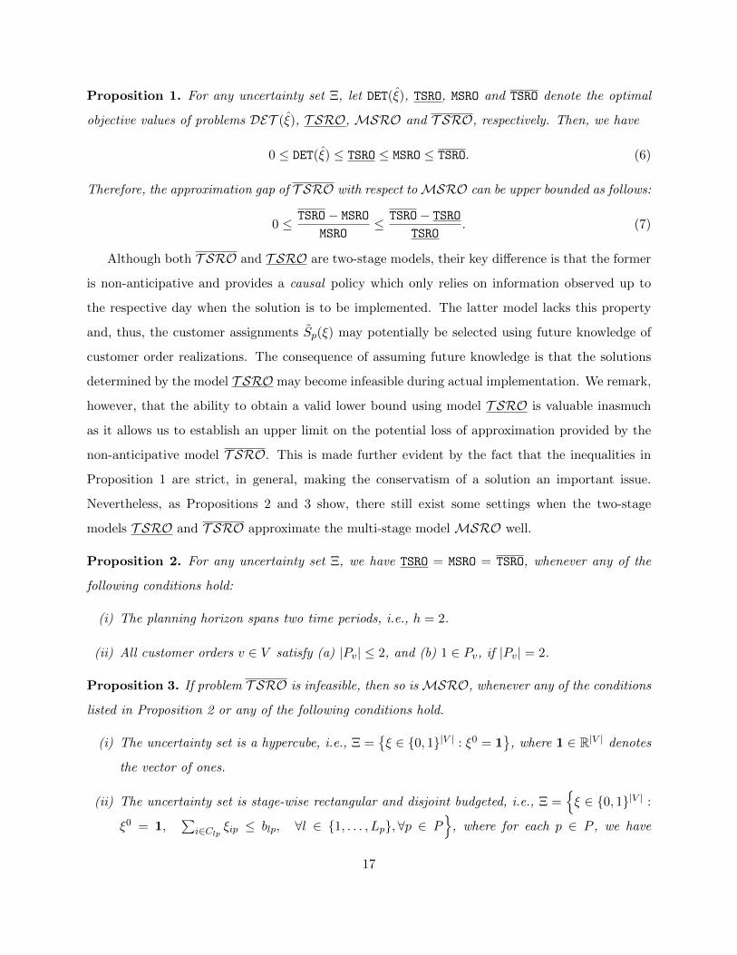
Proposition 1. For any uncertainty set Ξ, let DET(ξ), TSRO, MSRO and TSRO denote the optimal

objective values of problems DET (ξ), T SRO, MSRO and T SRO, respectively. Then, we have

0 ≤ DET(ξ) ≤ TSRO ≤ MSRO ≤ TSRO. (6)

Therefore, the approximation gap of T SRO with respect toMSRO can be upper bounded as follows:

0 ≤ TSRO− MSRO

MSRO≤ TSRO− TSRO

TSRO. (7)

Although both T SRO and T SRO are two-stage models, their key difference is that the former

is non-anticipative and provides a causal policy which only relies on information observed up to

the respective day when the solution is to be implemented. The latter model lacks this property

and, thus, the customer assignments Sp(ξ) may potentially be selected using future knowledge of

customer order realizations. The consequence of assuming future knowledge is that the solutions

determined by the model T SRO may become infeasible during actual implementation. We remark,

however, that the ability to obtain a valid lower bound using model T SRO is valuable inasmuch

as it allows us to establish an upper limit on the potential loss of approximation provided by the

non-anticipative model T SRO. This is made further evident by the fact that the inequalities in

Proposition 1 are strict, in general, making the conservatism of a solution an important issue.

Nevertheless, as Propositions 2 and 3 show, there still exist some settings when the two-stage

models T SRO and T SRO approximate the multi-stage model MSRO well.

Proposition 2. For any uncertainty set Ξ, we have TSRO = MSRO = TSRO, whenever any of the

following conditions hold:

(i) The planning horizon spans two time periods, i.e., h = 2.

(ii) All customer orders v ∈ V satisfy (a) |Pv| ≤ 2, and (b) 1 ∈ Pv, if |Pv| = 2.

Proposition 3. If problem T SRO is infeasible, then so isMSRO, whenever any of the conditions

listed in Proposition 2 or any of the following conditions hold.

(i) The uncertainty set is a hypercube, i.e., Ξ ={ξ ∈ {0, 1}|V | : ξ0 = 1

}, where 1 ∈ R|V | denotes

the vector of ones.

(ii) The uncertainty set is stage-wise rectangular and disjoint budgeted, i.e., Ξ ={ξ ∈ {0, 1}|V | :

ξ0 = 1,∑

i∈Clpξip ≤ blp, ∀l ∈ {1, . . . , Lp},∀p ∈ P

}, where for each p ∈ P , we have

17

Lp ∈ Z+, Clp ⊆ N and Clp ∩Cl′p = ∅ for l 6= l′; and, all customers i ∈ N with wi ≥ 2 satisfy

`i ≥ h, while all customers i ∈ N with wi = 1 satisfy ei = 1.

The settings referenced in Propositions 2 and 3 correspond to cases where customers don’t have

much flexibility in their day windows. For instance, condition (ii) of Proposition 3 states that the

two-stage model T SRO is a good approximation of the multi-stage model MSRO, if “flexible”

customers (those with at least two feasible service days, wi ≥ 2) request service sufficiently in

advance of the end of their day window (`i ≥ h), while “inflexible” customers (those with exactly

one feasible service day, wi = 1) request service only one day in advance (ei = 1). Moreover, it

can be shown that these results may fail to hold if the conditions stated in the above propositions

deviate only slightly. We do not present the relevant counterexamples for the sake of brevity.

It must be mentioned that all four models provide an order assignment for the next day, i.e,

day 1 (assuming the model has a feasible solution). We also note that, since each of these models

ignores information beyond the planning horizon, none of them can guarantee feasibility in a rolling

horizon context, in which they will be used (see Section 5.5). However, it should be highlighted

that the solutions determined by models DET (ξ) and T SRO can also become infeasible in a

folding horizon context, in which solutions are determined through models that are instantiated on

successively smaller subsets of the planning horizon and updated to reflect the actual realization of

the uncertainty. This is in contrast to model T SRO, which provides guarantees of robust feasibility

in this manner, and the example in Appendix B also illustrates this point.

Finally, we remark that, unlike the multi-stage model, whose numerical solution is challenging

to compute, we can develop efficient numerical schemes for models T SRO and T SRO. In the

following sections, we will provide such schemes and use them to quantify the gap between their

objective values for a wide range of problem instances in our numerical experiments.

Remark 3. The aforementioned models deviate from traditional robust optimization models be-

cause, amongst all robust feasible solutions, they select the one that minimizes the cost under a

particular uncertainty realization as opposed to the one that minimizes the worst-case cost. There

are several reasons for this modeling choice, the most important of them being the computational

intractability associated with the worst-case objective function. Indeed, simply evaluating the

worst-case routing cost of a fixed subset of orders selected to be serviced on some day, S ⊆ V ,

amounts to solving a computationally difficult bilevel optimization problem, maxξ∈Ξ

CVRP(S, ξ,m).

18

This is challenging both from a modeling and algorithmic viewpoint, because it entails defining

the VRP over a graph with |V0| + O(|N |h) nodes whose presence or absence is uncertain. In

contrast to this, we can use a simple lower bound to the bilevel problem, obtained by evaluating

CVRP(S, ξ,m) for a particular realization ξ ∈ Ξ of the uncertainty. We choose this realization to be

the nominal one, ξ, since it entails defining the VRP over a graph with only |V0| nodes, all of whom

have confirmed service. Notably, apart from being amenable to numerical solution, this choice of

the objective function has other advantages: (i) it provides a reasonable indication of the routing

cost associated with an assignment of customer orders to future days; (ii) it allows direct compar-

ison with the deterministic model DET (ξ), since the difference in the optimal objective values of

models T SRO and DET (ξ) is precisely the cost of being robust against vehicle capacity violations

(also known as the price of robustness, see Section 5.4); and, (iii) it empirically performs very well

for the practical problem at hand; i.e., in the context of a rolling horizon, it significantly reduces

the frequency of vehicle capacity violations without incurring higher routing costs (see Section 5.5).

3 Solution Method

In the previous section, we characterized the solutions to problem T SRO by the subset of customer

orders selected to be served on any given day. In practice, however, we shall use mathematical

models to describe these solutions through integer variables and numerical methods to obtain their

optimal values. Section 3.1 describes an integer programing formulation of model T SRO, while

Section 3.2 elaborates on a branch-and-cut framework for its numerical solution.

3.1 Mathematical Formulation

Recall that a solution to model T SRO is an assignment of customer orders to days. In the following,

we shall describe these assignments through binary variables yvp that record whether a customer

order v ∈ V is selected to be served in period p ∈ P . In particular, these variables will enforce the

following definition:

yvp = 1⇐⇒ v ∈ Sp (8)

19

Note that any feasible assignment S ∈ F induces unique values for yvp through this relationship.

Conversely, whenever the binary variables yvp, v ∈ V , p ∈ P satisfy the equation∑p∈P

yvp =∑p∈Pv

yvp = 1 ∀ v ∈ V, (9)

requiring each customer order to be served exactly once during the planning horizon within its day

window, the values of yvp also induce a unique assignment of customer orders to days, and we shall

denote this assignment by S(y).

In order to evaluate the cost of the solutions under scenario ξ, we will use integer variables xuvp

to indicate whether a vehicle serves order v ∈ V0 immediately after order u (or the depot 0) in period

p ∈ P . To simplify notation, we define E0 = {((i, d), (j, d′)) ∈ V0 × V0 : (i, j) ∈ E or i = j, d 6= d′}

as the subset of edges which cover the pending customer orders and over which it is sufficient to

define routing variables x in order to evaluate the objective function of model T SRO. Furthermore,

given a set of customer orders S ⊆ V0, we define E0(S) = {(u, v) ∈ E0 : u, v ∈ S, u 6= v} as the set of

edges that connect orders in S. Following standard vehicle routing modeling techniques, we derive

the following integer programming formulation that is valid for the deterministic model under the

nominal scenario DET (ξ). We will use it as a basis in order to derive a valid formulation for T SRO.

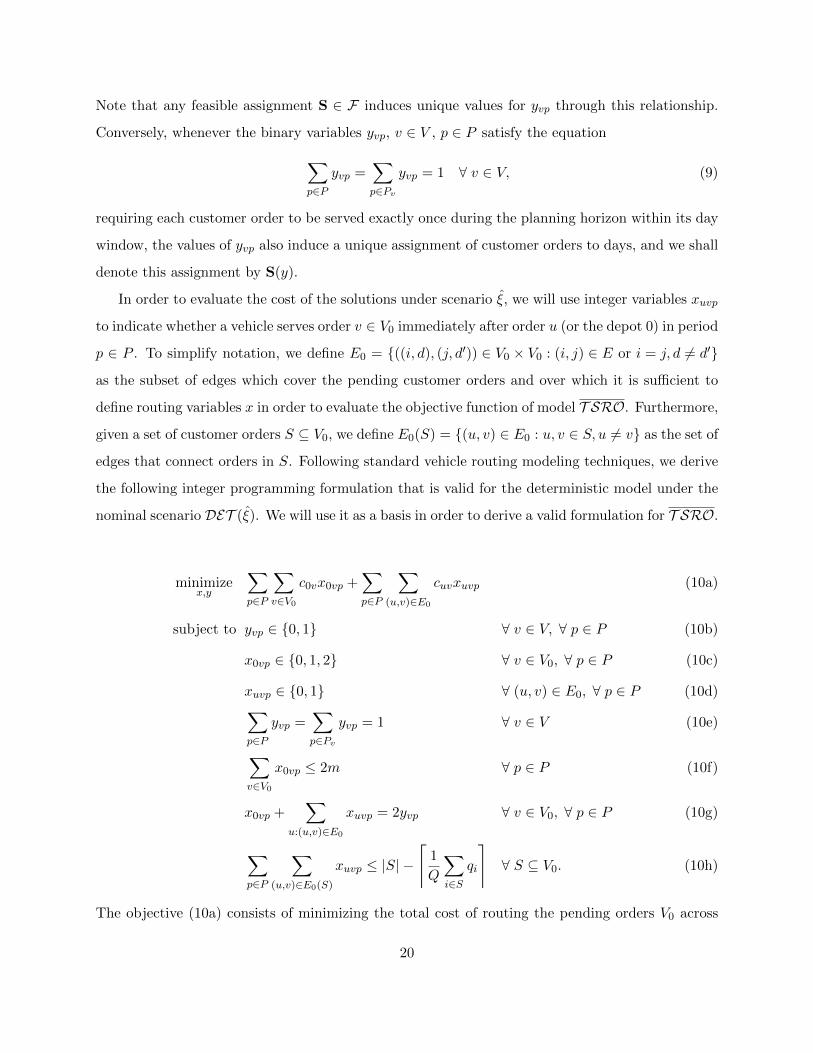
minimizex,y

∑p∈P

∑v∈V0

c0vx0vp +∑p∈P

∑(u,v)∈E0

cuvxuvp (10a)

subject to yvp ∈ {0, 1} ∀ v ∈ V, ∀ p ∈ P (10b)

x0vp ∈ {0, 1, 2} ∀ v ∈ V0, ∀ p ∈ P (10c)

xuvp ∈ {0, 1} ∀ (u, v) ∈ E0, ∀ p ∈ P (10d)∑p∈P

yvp =∑p∈Pv

yvp = 1 ∀ v ∈ V (10e)

∑v∈V0

x0vp ≤ 2m ∀ p ∈ P (10f)

x0vp +∑

u:(u,v)∈E0

xuvp = 2yvp ∀ v ∈ V0, ∀ p ∈ P (10g)

∑p∈P

∑(u,v)∈E0(S)

xuvp ≤ |S| −

⌈1

Q

∑i∈S

qi

⌉∀ S ⊆ V0. (10h)

The objective (10a) consists of minimizing the total cost of routing the pending orders V0 across

20

the planning horizon; equations (10e) stipulate that each known customer order must be served

exactly once within its day window; constraints (10f) require that no more than m vehicles depart

from the depot on any given day; equations (10g) state that, if customer order v ∈ V0 is served on

day p ∈ P , then there must be exactly two edges incident to v on day p. Finally, constraints (10h)

restrict subtours, requiring that each customer order is served by a vehicle that departs from and

returns to the depot, as well as enforce the vehicle capacity restrictions by imposing applicable

lower bounds on the number of vehicles that serve a set of orders S ⊆ V0.

In order for the binary variables yvp in the above formulation to induce a customer order

assignment S(y) that is robust feasible in T SRO, we must be able to serve Sp(y) using at most m

vehicles. We show that the following robust cover inequalities characterize the subsets of customer

orders that can be served in any period p ∈ P , Sp(y), such that S(y) is robust feasible in T SRO:

m+∑v∈S

(1− yvp) ≥ BPP(S, ξ) ∀ S ⊆ V, ∀ p ∈ P, ∀ ξ ∈ Ξ. (11)

Proposition 4. For any support Ξ and binary variables yvp, v ∈ V , p ∈ P , we have that

1. the robust cover inequalities (11) are necessary to induce a robust feasible customer order

assignment S(y) in T SRO; and

2. in conjunction with equations (9), the robust cover inequalities (11) are sufficient to induce

a robust feasible customer order assignment S(y) in T SRO.

Constraints (11) require that for every set S ⊆ V that is a subset of the customer orders

selected to be served in period p, the bin packing value associated with S under any realization

ξ ∈ Ξ must be no more than the number of vehicles available. For any candidate assignment Sp(y),

the left-hand side of the constraint associated with period p and S = Sp(y) evaluates to m, which

implies that there exists a capacity-feasible partition of Sp(y) into at most m components, for every

realization ξ ∈ Ξ. The formulation for T SRO, which we shall denote by T SROIP , is obtained by

appending constraints (11) to formulation (10).

3.2 Branch-and-Cut Framework

We use a branch-and-cut algorithm to solve formulation T SROIP . A branch-and-cut algorithm

embeds the addition of cutting planes within each tree node of a branch-and-bound algorithm.

21

The solution at the root node is obtained by solving the linear programming (LP) relaxation

consisting only of constraints (10e)–(10g) along with the variable bounds. Since the number of

constraints (10h) and (11) is exponential in the size of the instance, we remove these inequalities

and treat them in a cutting plane fashion by dynamically reintroducing them whenever the node

solution is found to violate them. Section 3.3 describes other families of inequalities that are valid

for the convex hull of integer feasible solutions of formulation T SROIP . Unlike constraints (10h)

and (11), these inequalities are not necessary to characterize the set of integer feasible solutions of

our formulation; however, they are capable of strengthening the LP relaxation in each node and,

therefore, can be used as cutting planes in order to expedite the search process.

Section 3.4 describes algorithms for solving the separation problems for inequalities (10h), (11)

and the other families of inequalities described in Section 3.3. When violated inequalities are

identified, the node solution is re-computed by adding all violated inequalities to the LP relaxation

and this procedure is iterated until no new inequalities are generated. If the final node solution

happens to satisfy all of the integrality constraints (10b)–(10d), then it is accepted as the new

incumbent solution since, in such cases, our algorithms for solving the separation problems for

inequalities (10h) and (11) are exact (i.e., they provide guarantees to identify a violating member,

if one exists). Otherwise, new sub-problems (i.e., nodes) are created by branching on an integer

variable whose value in the current node solution is fractional. The results in Section 5 have been

obtained by using the default branching strategy provided by the solver. Finally, since all identified

inequalities are valid globally (i.e., for all nodes of the branch-and-bound tree), we add them to the

LP relaxation of each open node of the tree.

3.3 Valid Inequalities

3.3.1 Lifted Robust Cover Inequalities

Observe that, if the right-hand side of the robust cover inequality (11) is not greater than m, then it

is dominated by the trivial variable bounds: 0 ≤ yvp ≤ 1. On the other hand, if its right-hand side is

strictly greater than m, then the following proposition shows that it is possible to lift the resulting

robust cover inequality. This lifting result is analogous to the lifting of valid cover inequalities for

the 0− 1 knapsack polytope to the so-called extended cover inequalities (see Balas [1975]). In this

proposition, C(S) := {v ∈ V \ S : qv ≥ max{qj : j ∈ S}} denotes the set of all customer orders with

22

higher demand than any order in S ⊆ V .

Proposition 5. For a customer order subset S ⊆ V , suppose that BPP(S, ξ) ≥ m + k is satisfied

for some ξ ∈ Ξ, where k ∈ N. Then, the following inequality is valid for formulation T SROIP :

∑v∈S

ξv (1− yvp)−∑

v∈C(S)

ξvyvp ≥ k ∀ p ∈ P. (12)

3.3.2 Robust Cumulative Capacity Inequalities

These inequalities enforce that the cumulative demand to be served in period p ∈ P , under any

customer order realization ξ ∈ Ξ, does not exceed the total fleet capacity mQ. Unlike the robust

cover inequalities (11), they ignore bin packing considerations and do not guarantee that the set

of customer orders selected to be served in period p can be packed into the available fleet. Nev-

ertheless, it can be shown that they do not dominate and are not dominated by the robust cover

inequalities (11); that is, node solutions of the branch-and-bound tree may violate them without

violating inequalities (11) and vice versa.

∑v∈V

qvξvyvp ≤ mQ ∀ p ∈ P, ∀ ξ ∈ Ξ. (13)

3.3.3 Valid Inequalities from CVRP

The two-index vehicle flow formulation is one of the most popular formulations for the CVRP. In this

formulation, integer variables x′ij count the number of times edge (i, j) is traversed by any vehicle in

a solution of the CVRP. Several families of inequalities are known to be valid for the corresponding

convex hull of integer feasible solutions, including the so-called rounded capacity, framed capacity,

strengthened comb, multistar and hypotour inequalities, among others (see Lysgaard et al. [2004]).

The following proposition shows that any such inequality can also be made valid for formulation (10)

by disaggregating (across periods) the corresponding edge variables that appear in the inequality.

Proposition 6. Let∑

(i,j)∈I λijx′ij ≤ µ be any inequality that is valid for the two-index formulation

of the CVRP instance defined on the subgraph of G with depot node 0, customers V0, demands qv,

v ∈ V0 and vehicle capacity Q. Then,∑

p∈P∑

(i,j)∈I λijxijp ≤ µ is valid for formulation (10).

Apart from the above inequalities, the following generalized subtour elimination constraints (14)

and generalized fractional capacity inequalities (15) are also valid for formulation (10). These

23

inequalities enforce lower bounds on the number of edges between S ⊆ V0 and its complement in

time period p ∈ P , whenever at least one member of S is served in period p. It can be shown that

they do not dominate and are not dominated by constraints (10h).

∑(u,v)∈E0(S)

xuvp ≤ |S| − yvp ∀ S ⊆ V0, ∀ v ∈ S, ∀ p ∈ P. (14)

∑(u,v)∈E0(S)

xuvp ≤ |S| −

(1

Q

∑v∈S

qvyvp

)∀ S ⊆ V0, ∀ p ∈ P. (15)

3.4 Separation Algorithms

3.4.1 Robust Cover Inequalities

Since the bin packing problem is NP-hard, the separation problem for inequalities (11) is also

NP-hard, even if Ξ consists of a single element. This motivates the need for separation heuristics.

Nevertheless, as mentioned previously, in the context of a branch-and-cut algorithm, the procedure

to solve these separation problems must be exact if the current node solution satisfies all of the

integrality constraints (10b)–(10d). Otherwise, a heuristic procedure to identify violated inequali-

ties suffices. In the following, we describe procedures to solve the associated separation problems

separately for the cases when the node solution is integral (i.e., satisfies (10b)–(10d)) or fractional.

For the remainder of this section, we shall assume that (x∗, y∗) is the current node solution for

which we want to identify violated robust cover inequalities.

We remark that we do not explicitly separate the lifted robust cover inequalities (12). Instead,

we use Proposition 5 to lift any identified violating member of (11) and add the lifted form of the

inequality to the current node solution.

Fractional Node Solutions: Typically, fractional node solutions are encountered much more

frequently in the branch-and-bound tree than those with integral solutions. Therefore, the separa-

tion procedures employed at such nodes must be computationally efficient, although not necessarily

exact. In this context, note that inequality (11) remains valid if we replace its right-hand side with

a lower bound. In the following, we attempt to separate the following relaxed version of the robust

cover inequalities (11), obtained by replacing the optimal value of the bin packing problem with

the so-called L1 lower bound [Martello and Toth, 1990]. We remark that, although the L1 bound

24

of the bin packing problem may deviate from its optimal value by up to 50% in the worst case, it

is typically tight when the item weights are sufficiently small with respect to the bin capacity.

m+∑v∈S

(1− yvp) ≥

⌈1

Q

∑v∈S

qvξv

⌉∀ S ⊆ V, ∀ p ∈ P, ∀ ξ ∈ Ξ. (11′)

Observe that there always exists a maximally violating member of the family of inequalities (11′)

satisfying ξv = 1 for all v ∈ S. Indeed, consider a member of (11′) defined by S ⊆ V , p ∈ P and

ξ ∈ Ξ such that ξv = 0 holds for some v ∈ S. Then, we can obtain a more violated member defined

by the same p and ξ but considering the subset S \ {v}: the right-hand side of this inequality is

the same as that of S, while its left-hand side can only decrease with respect to S. With this

observation, the separation problem for inequalities (11′), for a given p ∈ P , can be formulated as

the following binary program, where the variable zv ∈ {0, 1} indicates whether v ∈ S.

minimizez∈{0,1}|V |,ξ∈Ξ

{∑v∈V

(1− y∗vp)zv : z ≤ ξ,∑v∈V

qvzv ≥ mQ+ ε

}(16)

If (16) happens to be infeasible, then no violations are possible for the given p ∈ P . Otherwise,

if m +∑

v∈S∗(1 − y∗vp) >⌈∑

v∈S∗ qv/Q⌉

is satisfied, where S∗ = {v ∈ V : z∗v = 1} is defined by

the optimal solution (z∗, ξ∗) of (16), then the member of (11′) defined by S∗ and realization ξ∗

corresponds to a most violated inequality. Note that, without loss of optimality, we can fix to zero

all variables zv such that y∗vp = 0. This is because zv = 1 implies that the violation of the resulting

inequality corresponding to S∗ would only decrease with respect to that corresponding to S∗ \ {v}.

Observe that, for fixed ξ ∈ Ξ, (16) reduces to a standard knapsack problem, which typically

can be solved very efficiently by means of specialized algorithms [Martello and Toth, 1990]. In any

case, our computational experience with the instances solved in Section 5 suggested that the optimal

solution of problem (16) can be obtained very easily by using a commercial integer programming

solver, and the results in that section were therefore obtained in this manner.

Integral Node Solutions: For each p ∈ P , Sp(y∗) = {v ∈ V : y∗vp = 1} is the candidate set of

orders selected to be served in period p in the current node solution. In order to identify violated

inequalities in period p, it is sufficient to consider the inequality for S = Sp(y∗). This is because:

(i) for any subset of S, the left-hand side of (11) evaluated at the current node solution remains the

same as for S, while the right-hand side can only decrease with respect to that for S; (ii) for any

25

set S ∪ {v}, where v ∈ V is such that y∗vp = 0, the left-hand side of (11) evaluated at the current

node solution increases by one (with respect to S) while the right-hand side increases by at most

one. In either case, the magnitude of violation of the resulting inequality can never increase with

respect to that for S. Stated differently, the current node solution maximally violates the member

of (11) corresponding to S = Sp(y∗), for given p ∈ P and ξ ∈ Ξ. For this choice of S, the left-hand

side of (11) evaluates to m and satisfaction of the inequality is equivalent to checking if

m ≥ BPP(S, ξ∗),where ξ∗ ∈ arg maxξ∈Ξ

BPP(S, ξ).

If m < BPP(S, ξ∗), then the inequality corresponding to set S, period p and customer order real-

ization ξ∗ is added to the current node solution. If no violations are found in any p ∈ P , then the

current node solution is guaranteed to satisfy each member of (11).

The computation of a maximizer of BPP(S, ξ) needs to be done as often as the branch-and-bound

tree encounters integral node solutions and, hence, it is crucial that this can be done efficiently. For

general supports Ξ, this requires the solution of a bilevel integer program in which the (upper level)

problem is to determine a scenario ξ ∈ Ξ that maximizes the optimal value of the (lower level)

bin packing problem BPP(S, ξ). It is computationally difficult to solve this problem using existing

methods (e.g., see DeNegre and Ralphs [2009], Zeng and An [2014], Tang et al. [2016]), since

they typically do not address problems containing bilinear terms between upper and lower level

decisions. In order to address this and other limitations, we present in Appendix C a numerically

efficient solution procedure that improves upon and extends the column-and-constraint generation

framework [Zhao and Zeng, 2012] for solving such problems. By formulating the lower-level bin

packing problem as a feasibility problem, the proposed procedure does not necessarily compute a

maximizer of BPP(S, ξ). Instead, it either certifies that BPP(S, ξ∗) ≤ m, or returns a realization ξ

for which BPP(S, ξ) > m. In either case, the exactness of the separation procedure is guaranteed.

We remark that the procedure presented above can address any uncertainty set Ξ that satisfies

the conditions (C1)–(C3) described in Section 2. It turns out that, for specially structured disjoint

budget uncertainty sets of the type shown in (2), we can compute a maximizer of BPP(S, ξ) more

efficiently, avoiding the solution of a bilevel program.

Proposition 7. Assume that the uncertainty set Ξ is of type (2) and disjoint budgeted. Also,

for any S ⊆ V and l = 1, . . . , L, assume that vl,1, vl,2, . . . , vl,|S∩Bl| represents an ordering of the

26

customer orders in the set S∩Bl according to non-increasing demand; that is, qvl,1 ≥ . . . ≥ qvl,|S∩Bl|.

Let J0 := V0∪S\∪Ll=1Bl; and, for l = 1, . . . , L, let Jl := {vl,1, . . . , vl,jl}, where jl = min{bl, |S ∩Bl|}.

Then, an optimal solution ξ∗ of max {BPP(S, ξ) : ξ ∈ Ξ} is given by

ξ∗v =

1, if v ∈ J0 ∪ J1 ∪ . . . ∪ JL

0 otherwisefor all v ∈ V.

With suitably chosen data structures, Proposition 7 shows that we can obtain a maximizer ξ∗

of the right-hand side of inequality (11) for a given S ⊆ V in time O(|S| +∑L

l=1 bl log bl) using a

partial sorting algorithm. Once the maximizer is obtained, a deterministic bin packing problem

BPP(S, ξ∗) must be solved in order to check if a violation exists. In our implementation, we solved

these bin packing problems using the exact algorithm MTP described in Martello and Toth [1990].

3.4.2 Robust Cumulative Capacity Inequalities

For fixed p ∈ P , the separation problem for the robust cumulative capacity inequalities (13) can be

formulated as a binary program: max{∑

v∈V qvy∗vpξv : ξ ∈ Ξ

}. Here, (x∗, y∗) represents the current

node solution. If∑

v∈V qvy∗vpξ∗v > mQ is satisfied, where ξ∗ is the optimal solution of the binary

program, then the inequality (13) corresponding to period p and customer order realization ξ∗ is

violated. As in the case of the robust cover inequalities, for disjoint budget uncertainty sets, the

solution of a binary program can be avoided. In such cases, a slight modification of Proposition 7

allows us to compute ξ∗ in time O(|V |+∑L

l=1 bl log bl). Specifically, we apply Proposition 7 to the

set S = V but, instead of ordering the elements in the set S ∩Bl = V ∩Bl = Bl by non-increasing

demand, we order them by non-increasing values of qvy∗vp.

3.4.3 Valid Inequalities from CVRP

Proposition 6 shows that any family of valid inequalities for the CVRP can be made valid for

formulation T SROIP . Violated members of these families of inequalities (including (10h)) can be

identified using the same observation. Specifically, given the current node solution (x∗, y∗), compute

the corresponding two-index solution: x′∗ij =∑

p∈P x∗ijp for each (i, j). The resulting vector x′∗ can

then be used as input to any separation algorithm for the corresponding family of inequalities.

In our implementation, we used the CVRPSEP package [Lysgaard et al., 2004] for separating

inequalities (10h) along with the framed capacity, comb, multistar and hypotour inequalities. 0.

27

The generalized subtour elimination constraints (14) can be separated in polynomial time by solving

|V0| maximum flow problems. We refer the reader to Fischetti et al. [1998] for details, wherein a

procedure to generate more than one violated inequality is also described; the results in Section 5

were obtained using this procedure. The separation problem for the generalized fractional capacity

inequalities can also be solved in polynomial time because it reduces to the separation problem for

the standard fractional capacity inequalities for the CVRP after modifying the customer demands

to be qvy∗vp for each v ∈ V0. McCormick et al. [2003] describe routines for solving the associated

separation problems, which we also used in obtaining the results of Section 5.

4 Computation of Lower Bounds

Proposition 1 shows that we can bound from below the optimal value of model MSRO and,

hence, of T SRO via the optimal value of T SRO. Therefore, using this value, we can quantify

how well T SRO approximates MSRO. In this section, we discuss how to numerically compute

the optimal value of T SRO. The approach is a branch-and-cut algorithm similar to that for

solving T SRO and much of the discussion mirrors Sections 3.1 and 3.2; therefore, we only emphasize

the aspects which differ in the two cases.

4.1 Mathematical Formulation

Formulation (10) serves as the basis of an integer programming model for T SRO, which we shall de-

note by T SROIP . While the interpretation of binary variables yvp was straightforward in T SROIP ,

in the case of T SROIP , variables yvp will indicate whether customer order v ∈ V is selected to

be served in period p ∈ P in the customer order assignment obtained by evaluating the optimal

solution policy under scenario ξ:

yv1 = 1⇐⇒ i ∈ S1

yvp = 1⇐⇒ i ∈ Sp(ξ) for all p ∈ P \ {1}.(17)

Note that any solution (S1, S2(·), . . . , Sh(·)) of T SRO induces unique values for yvp through this

relationship. Conversely, whenever the binary variables yvp satisfy equation (9), their values induce

a unique assignment on day 1, which we shall denote by S1(y), that would be common across all

feasible customer order assignments (S1, S2(·), . . . , Sh(·)). However, rather than construct explicit

28

functional forms of Sp(·), formulation T SROIP only enforces the existence of one. The existence of

a feasible solution in T SRO is equivalent to the existence of feasible assignments for all realizations

of the uncertainty, with the additional restriction that they must share the same here-and-now

assignment, S1(y). This, in turn, is equivalent to the existence of a capacity-feasible and day

window-feasible partition of the orders V \S1(y) into h−1 subsets, S2(ξ), . . . , Sh(ξ), for each ξ ∈ Ξ.

Motivated by this observation, for any S ⊆ V \ {v ∈ V : Pv = {1}}, and for any ξ ∈ Ξ, let

BPPDW(S, ξ) denote the optimal value of an instance of the Bin Packing Problem with Day Windows.

In this problem, the bin size is Q, the set of days is P \ {1}, and the items are the elements of

S featuring weights qvξv and day windows Pv \ {1} for each v ∈ S. Further, at least m (possibly

empty) bins must be used used on each day p ∈ P \ {1}. The requirement of using at least m bins

on each day is necessary to disallow the case where the optimal solution of the bin packing problem

uses less than m(h−1) bins overall, but more than m bins on some day. We show that the following

robust cover inequalities characterize the sets of here-and-now customer order assignments that can

be part of a feasible solution in T SRO:

m(h− 1) +∑v∈S

yv1 ≥ BPPDW(S, ξ) ∀ S ⊆ V \ {v ∈ V : Pv = {1}} , ∀ ξ ∈ Ξ. (18)

Proposition 8. For any support Ξ and binary variables yvp, v ∈ V , p ∈ P , we have that

1. the robust cover inequalities (18) are necessary to induce a customer order assignment on

day 1, S1(y), that guarantees the existence of a feasible solution (S1(y), S2(·), . . . , Sh(·)) in

T SRO.

2. in conjunction with equations (9), the robust cover inequalities (11) are sufficient to induce a

customer order assignment on day 1, S1(y), that guarantees the existence of a feasible solution

(S1(y), S2(·), . . . , Sh(·)) in T SRO.

Constraints (18) require that, for every set S ⊆ V that is a subset of the customer orders selected

to be served on days other than day 1, the bin packing value associated with S (considering day

windows) under any realization ξ ∈ Ξ must be no more than the total number of vehicles available

over the planning horizon. For any assignment S1(y), the left hand side of the constraint associated

with S = V \S1(y) evaluates to m(h−1), which implies that there exists a capacity feasible partition

of V \S1(y) into h−1 solutions, each containing at most m components, for every realization ξ ∈ Ξ.

The formulation for T SRO is obtained by adding constraints (18) to formulation (10).

29

Remark 4. The Bin Packing Problem with Day Windows can be viewed as a special case of the

well-studied Bin Packing Problem with Conflicts [Jansen and Ohring, 1997] and may be modeled

as such, albeit with an additional restriction that accounts for using at least m bins on each day.

Indeed, given any instance of the former, we can construct an instance of the latter by using the

same set of items, the same bin size and constructing the so-called “conflict graph” by defining

edges (u, v) whenever Pu ∩Pv = ∅, for u and v in the set of items. However, without the additional

restriction of using at least m bins on each day, the resulting instance of the Bin Packing Problem

with Conflicts constitutes only a relaxation of the Bin Packing Problem with Day Windows.

4.2 Branch-and-Cut Framework

We use a branch-and-cut algorithm to solve formulation T SROIP . The initial LP relaxation

consists of constraints (10e)–(10g) along with variable bounds. Constraints (10h) and (18) are

removed and are dynamically reintroduced as cutting planes whenever the node solution is found

to violate them. The CVRP inequalities described in Section 3.3.3 are valid for T SROIP as well

and can be used in the branch-and-cut algorithm as cutting planes. Similarly, the robust cumulative

capacity inequalities described in Section 3.3.2 are also valid, albeit with a slight modification, as

follows. ∑v∈V

qvξv(1− yv1) ≤ m(h− 1)Q ∀ ξ ∈ Ξ. (19)

These inequalities enforce that the total demand to be served on days other than day 1, under any

customer order realization ξ ∈ Ξ, does not exceed the total fleet capacity available on those days.

The procedure to solve the separation problem for these inequalities is similar to that described in

Section 3.4.2. Finally, it can also be shown that they do not dominate and are not dominated by

the robust cover inequalities (18).

The remainder of this section describes our separation procedures for the robust cover inequal-

ities (18) employed within the branch-and-cut algorithm. We shall assume that (x∗, y∗) is the

current node solution for which we want to identify violated inequalities. If the current node solu-

tion happens to be fractional, i.e., does not satisfy constraints (10b)–(10d), then we can relax the

robust cover inequality (18) and replace its right-hand side with a valid lower bound. For example,

the L1 bound described in Section 3.4.1 is a valid lower bound for the bin packing problem with day

windows as well, and the procedure described therein can be utilized to solve the separation prob-

30

lems of the corresponding relaxed version of inequalities (18). Similarly, Remark 4 shows that we

can utilize lower bounds to the bin packing problem with conflicts [Gendreau et al., 2004] to derive

valid relaxations of the robust inequalities (18). However, preliminary computational experiments

showed that these lower bounds are typically weak and that it does not pay off to expend additional

computational effort in separating the relaxed inequalities as they are almost never violated.

On the other hand, if the current node solution happens to be integral, i.e., satisfies con-

straints (10b)–(10d), then the separation procedure for the robust cover inequalities (18) must be

exact. In such cases, S1(y∗) = {v ∈ V : y∗v1 = 1} is the candidate set of customer orders selected

to be served on day 1. By a similar argument as in Section 3.4.1, it can be shown that the current

node solution maximally violates the member of the family of inequalities (18) corresponding to

S = V \S1(y∗), for given ξ ∈ Ξ. For this choice of S, the left-hand side of (18) evaluates to m(h−1)

and satisfaction of the inequality is equivalent to checking if

m(h− 1) ≥ BPPDW(S, ξ∗),where ξ∗ ∈ arg maxξ∈Ξ

BPPDW(S, ξ).

Ifm(h−1) < BPPDW(S, ξ∗), then the inequality corresponding to set S and customer order realization

ξ∗ is violated. The computation of ξ∗ requires the solution of a bilevel integer program, for which we

use the procedure described in Appendix C. By formulating the bin packing problem as a feasibility

problem, the procedure either certifies that BPPDW(S, ξ∗) ≤ m(h− 1), or returns a realization ξ for

which BPPDW(S, ξ) > m(h− 1), thus guaranteeing the exactness of the separation procedure.

5 Computational Experiments

This section presents computational results obtained using the branch-and-cut algorithms described

in Sections 3.2 and 4.2 on benchmark instances from the literature. Specifically, in Section 5.1, we

present the characteristics of the test instances; in Section 5.2, we present a summary of the nu-

merical performance of our algorithm; in Section 5.3, we present detailed tables of results outlining

the effect of the various inequalities; in Section 5.4, we analyze the approximation quality of our

two-stage model; and finally, in Section 5.5, we study the performance of the proposed robust op-

timization model in a rolling horizon simulation framework, and we compare it to the performance

of the deterministic model as well as two decision approaches that are popular among practitioners.

The algorithms were implemented in C++ using the C callable library of CPLEX 12.7 and

31

compiled with the GCC 5.1.0 compiler. The experiments were conducted on a single-core of an

Intel Xeon 3.1 GHz processor with a software imposed memory limit of 6 GB. In the implementa-

tion of the algorithms, all CPLEX-generated cutting planes were disabled because enabling them

increased overall computation times; all other solver options were left at their default values. In-

terested readers can freely download our code implementation, datasets used, and associated user

instructions in the following link: http://gounaris.cheme.cmu.edu/codes/mpvrp.

5.1 Test Instances

Our instances are derived from the standard CVRP benchmark instances in the so-called A, B,

E, F, M and P datasets,10 which are usually adopted to generate benchmark instances for several

variants of the vehicle routing problem. The number of customer nodes in these CVRP instances

range from 12 to 199. From each of these CVRP instances, we generate a single multi-period VRP

instance using the procedure described in Baldacci et al. [2011]. Since the work of Baldacci et al.

[2011] does not study the problem in the context of the longer (possibly infinite) time horizon Π,

we interpret the resulting five-period VRP instance (i.e., h = 5) as a possible instantiation of the

deterministic model to be solved at the end of day 0 of the longer horizon. Specifically, we let V0 be

the set of pending orders as specified in Baldacci et al. [2011], and we let N be the set of customers

in the original CVRP instance. For each i ∈ N , qi is set equal to the demand in the original

instance; ei is sampled uniformly in [ρi, h], where ρi is the first day of the day window {ρi, . . . , δi}

as specified in Baldacci et al. [2011];11 and, `i is set to be ei + wi − 1, where the width wi is set

equal to the original width, δi − ρi + 1, if ρi > 1, and is uniformly sampled in [δi, 3] otherwise. In

the resulting instance, the average width of a day window (= wi) is 2, and the average number of

days elapsed between the day at which an order is placed and the first feasible service day (= ei) is

3.5, which are similar to the corresponding values (2.5 and 2.5 respectively) in the real world case

study of Wen et al. [2010]. Finally, we note that we set the vehicle capacity Q equal to the value

in the original CVRP instance, and we round the transportation costs c up to the nearest integer.

To construct meaningful uncertainty sets Ξ, we assume that each customer i ∈ N can place a

service request on any day of the horizon with probability α ∈ [0, 1]. We then consider the following

10See Lysgaard et al. [2004] for references to the original sources of these datasets.11We allow for the possibility that ei 6= ρi, since the effective day window might have been shrunk in the context of

the longer horizon Π (see footnote 5).

32

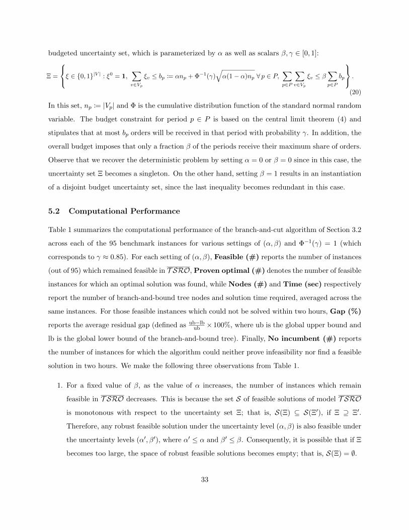
budgeted uncertainty set, which is parameterized by α as well as scalars β, γ ∈ [0, 1]:

Ξ =

ξ ∈ {0, 1}|V | : ξ0 = 1,∑v∈Vp

ξv ≤ bp := αnp + Φ−1(γ)√α(1− α)np ∀ p ∈ P,

∑p∈P

∑v∈Vp

ξv ≤ β∑p∈P

bp

.

(20)

In this set, np := |Vp| and Φ is the cumulative distribution function of the standard normal random

variable. The budget constraint for period p ∈ P is based on the central limit theorem (4) and

stipulates that at most bp orders will be received in that period with probability γ. In addition, the

overall budget imposes that only a fraction β of the periods receive their maximum share of orders.

Observe that we recover the deterministic problem by setting α = 0 or β = 0 since in this case, the

uncertainty set Ξ becomes a singleton. On the other hand, setting β = 1 results in an instantiation

of a disjoint budget uncertainty set, since the last inequality becomes redundant in this case.

5.2 Computational Performance

Table 1 summarizes the computational performance of the branch-and-cut algorithm of Section 3.2

across each of the 95 benchmark instances for various settings of (α, β) and Φ−1(γ) = 1 (which

corresponds to γ ≈ 0.85). For each setting of (α, β), Feasible (#) reports the number of instances

(out of 95) which remained feasible in T SRO, Proven optimal (#) denotes the number of feasible

instances for which an optimal solution was found, while Nodes (#) and Time (sec) respectively

report the number of branch-and-bound tree nodes and solution time required, averaged across the

same instances. For those feasible instances which could not be solved within two hours, Gap (%)

reports the average residual gap (defined as ub−lbub × 100%, where ub is the global upper bound and

lb is the global lower bound of the branch-and-bound tree). Finally, No incumbent (#) reports

the number of instances for which the algorithm could neither prove infeasibility nor find a feasible

solution in two hours. We make the following three observations from Table 1.

1. For a fixed value of β, as the value of α increases, the number of instances which remain

feasible in T SRO decreases. This is because the set S of feasible solutions of model T SRO

is monotonous with respect to the uncertainty set Ξ; that is, S(Ξ) ⊆ S(Ξ′), if Ξ ⊇ Ξ′.

Therefore, any robust feasible solution under the uncertainty level (α, β) is also feasible under

the uncertainty levels (α′, β′), where α′ ≤ α and β′ ≤ β. Consequently, it is possible that if Ξ

becomes too large, the space of robust feasible solutions becomes empty; that is, S(Ξ) = ∅.

33

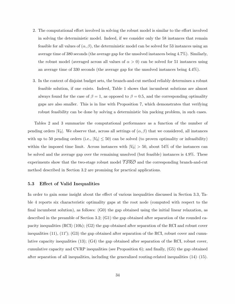
2. The computational effort involved in solving the robust model is similar to the effort involved

in solving the deterministic model. Indeed, if we consider only the 58 instances that remain

feasible for all values of (α, β), the deterministic model can be solved for 53 instances using an

average time of 380 seconds (the average gap for the unsolved instances being 4.7%). Similarly,

the robust model (averaged across all values of α > 0) can be solved for 51 instances using

an average time of 330 seconds (the average gap for the unsolved instances being 4.4%).

3. In the context of disjoint budget sets, the branch-and-cut method reliably determines a robust

feasible solution, if one exists. Indeed, Table 1 shows that incumbent solutions are almost

always found for the case of β = 1, as opposed to β = 0.5, and the corresponding optimality

gaps are also smaller. This is in line with Proposition 7, which demonstrates that verifying

robust feasibility can be done by solving a deterministic bin packing problem, in such cases.

Tables 2 and 3 summarize the computational performance as a function of the number of

pending orders |V0|. We observe that, across all settings of (α, β) that we considered, all instances

with up to 50 pending orders (i.e., |V0| ≤ 50) can be solved (to proven optimality or infeasibility)

within the imposed time limit. Across instances with |V0| > 50, about 54% of the instances can

be solved and the average gap over the remaining unsolved (but feasible) instances is 4.9%. These

experiments show that the two-stage robust model T SRO and the corresponding branch-and-cut

method described in Section 3.2 are promising for practical applications.

5.3 Effect of Valid Inequalities

In order to gain some insight about the effect of various inequalities discussed in Section 3.3, Ta-

ble 4 reports six characteristic optimality gaps at the root node (computed with respect to the

final incumbent solution), as follows: (G0) the gap obtained using the initial linear relaxation, as

described in the preamble of Section 3.2; (G1) the gap obtained after separation of the rounded ca-

pacity inequalities (RCI) (10h); (G2) the gap obtained after separation of the RCI and robust cover

inequalities (11), (11′); (G3) the gap obtained after separation of the RCI, robust cover and cumu-

lative capacity inequalities (13); (G4) the gap obtained after separation of the RCI, robust cover,

cumulative capacity and CVRP inequalities (see Proposition 6); and finally, (G5) the gap obtained

after separation of all inequalities, including the generalized routing-related inequalities (14)–(15).

34

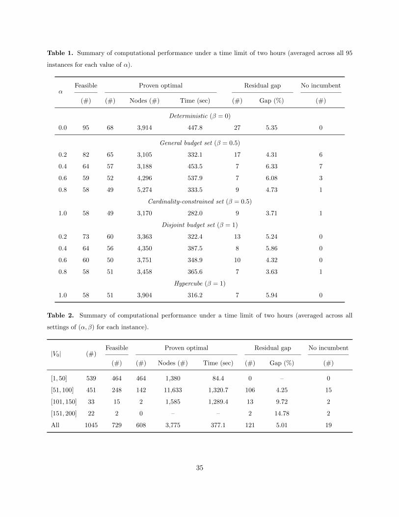
Table 1. Summary of computational performance under a time limit of two hours (averaged across all 95

instances for each value of α).

αFeasible Proven optimal Residual gap No incumbent

(#) (#) Nodes (#) Time (sec) (#) Gap (%) (#)

Deterministic (β = 0)

0.0 95 68 3,914 447.8 27 5.35 0

General budget set (β = 0.5)

0.2 82 65 3,105 332.1 17 4.31 6

0.4 64 57 3,188 453.5 7 6.33 7

0.6 59 52 4,296 537.9 7 6.08 3

0.8 58 49 5,274 333.5 9 4.73 1

Cardinality-constrained set (β = 0.5)

1.0 58 49 3,170 282.0 9 3.71 1

Disjoint budget set (β = 1)

0.2 73 60 3,363 322.4 13 5.24 0

0.4 64 56 4,350 387.5 8 5.86 0

0.6 60 50 3,751 348.9 10 4.32 0

0.8 58 51 3,458 365.6 7 3.63 1

Hypercube (β = 1)

1.0 58 51 3,904 316.2 7 5.94 0

Table 2. Summary of computational performance under a time limit of two hours (averaged across all

settings of (α, β) for each instance).

|V0| (#)Feasible Proven optimal Residual gap No incumbent

(#) (#) Nodes (#) Time (sec) (#) Gap (%) (#)

[1, 50] 539 464 464 1,380 84.4 0 – 0

[51, 100] 451 248 142 11,633 1,320.7 106 4.25 15

[101, 150] 33 15 2 1,585 1,289.4 13 9.72 2

[151, 200] 22 2 0 – – 2 14.78 2

All 1045 729 608 3,775 377.1 121 5.01 19

35

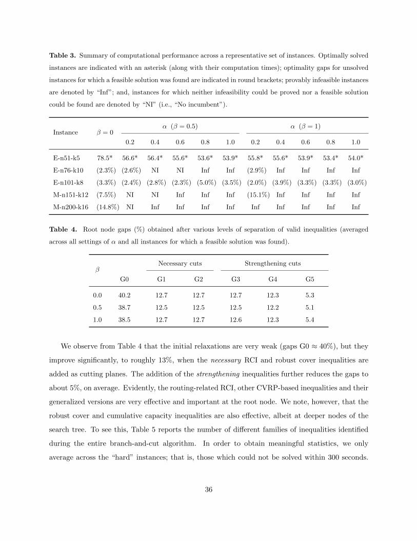
Table 3. Summary of computational performance across a representative set of instances. Optimally solved

instances are indicated with an asterisk (along with their computation times); optimality gaps for unsolved

instances for which a feasible solution was found are indicated in round brackets; provably infeasible instances

are denoted by “Inf”; and, instances for which neither infeasibility could be proved nor a feasible solution

could be found are denoted by “NI” (i.e., “No incumbent”).

Instance β = 0α (β = 0.5) α (β = 1)

0.2 0.4 0.6 0.8 1.0 0.2 0.4 0.6 0.8 1.0

E-n51-k5 78.5* 56.6* 56.4* 55.6* 53.6* 53.9* 55.8* 55.6* 53.9* 53.4* 54.0*

E-n76-k10 (2.3%) (2.6%) NI NI Inf Inf (2.9%) Inf Inf Inf Inf

E-n101-k8 (3.3%) (2.4%) (2.8%) (2.3%) (5.0%) (3.5%) (2.0%) (3.9%) (3.3%) (3.3%) (3.0%)

M-n151-k12 (7.5%) NI NI Inf Inf Inf (15.1%) Inf Inf Inf Inf

M-n200-k16 (14.8%) NI Inf Inf Inf Inf Inf Inf Inf Inf Inf

Table 4. Root node gaps (%) obtained after various levels of separation of valid inequalities (averaged

across all settings of α and all instances for which a feasible solution was found).

βNecessary cuts Strengthening cuts

G0 G1 G2 G3 G4 G5

0.0 40.2 12.7 12.7 12.7 12.3 5.3

0.5 38.7 12.5 12.5 12.5 12.2 5.1

1.0 38.5 12.7 12.7 12.6 12.3 5.4

We observe from Table 4 that the initial relaxations are very weak (gaps G0 ≈ 40%), but they

improve significantly, to roughly 13%, when the necessary RCI and robust cover inequalities are

added as cutting planes. The addition of the strengthening inequalities further reduces the gaps to

about 5%, on average. Evidently, the routing-related RCI, other CVRP-based inequalities and their

generalized versions are very effective and important at the root node. We note, however, that the

robust cover and cumulative capacity inequalities are also effective, albeit at deeper nodes of the

search tree. To see this, Table 5 reports the number of different families of inequalities identified

during the entire branch-and-cut algorithm. In order to obtain meaningful statistics, we only

average across the “hard” instances; that is, those which could not be solved within 300 seconds.

36

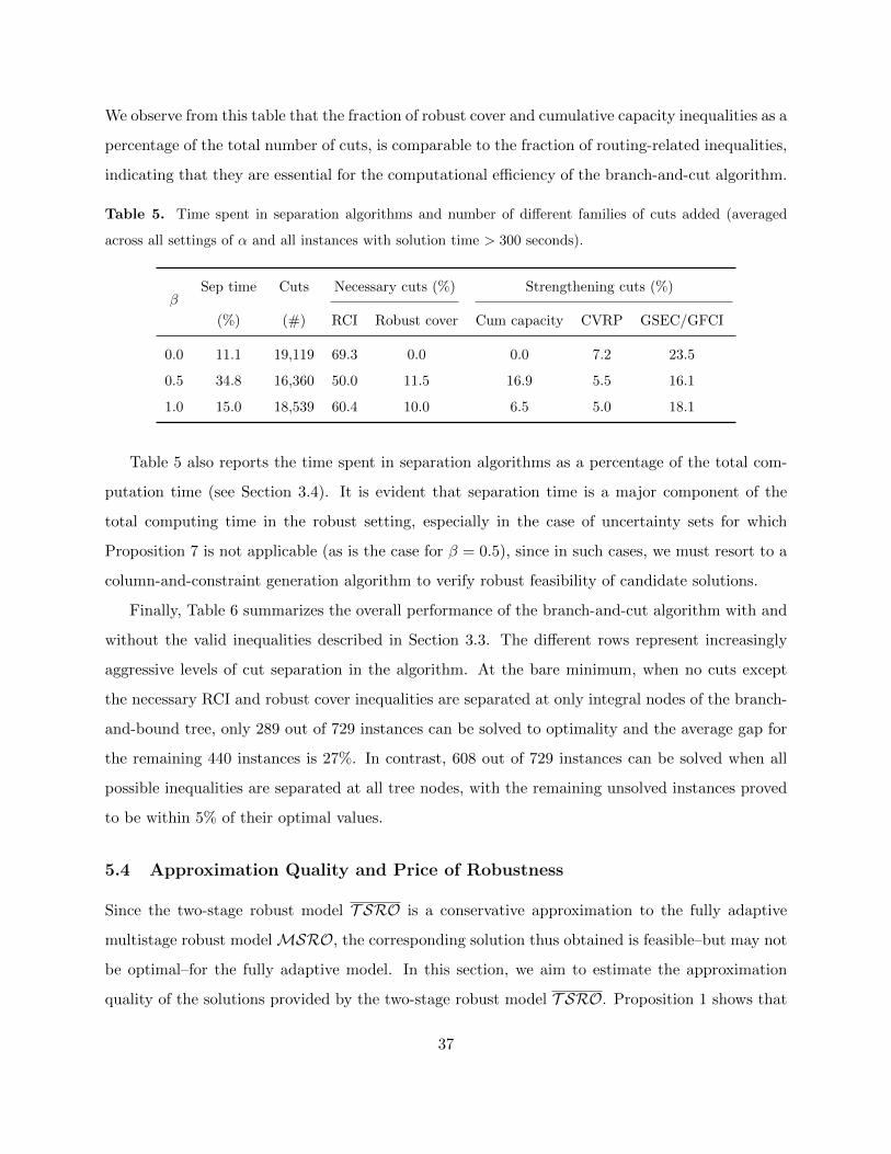
We observe from this table that the fraction of robust cover and cumulative capacity inequalities as a

percentage of the total number of cuts, is comparable to the fraction of routing-related inequalities,

indicating that they are essential for the computational efficiency of the branch-and-cut algorithm.

Table 5. Time spent in separation algorithms and number of different families of cuts added (averaged

across all settings of α and all instances with solution time > 300 seconds).

βSep time Cuts Necessary cuts (%) Strengthening cuts (%)

(%) (#) RCI Robust cover Cum capacity CVRP GSEC/GFCI

0.0 11.1 19,119 69.3 0.0 0.0 7.2 23.5

0.5 34.8 16,360 50.0 11.5 16.9 5.5 16.1

1.0 15.0 18,539 60.4 10.0 6.5 5.0 18.1

Table 5 also reports the time spent in separation algorithms as a percentage of the total com-

putation time (see Section 3.4). It is evident that separation time is a major component of the

total computing time in the robust setting, especially in the case of uncertainty sets for which

Proposition 7 is not applicable (as is the case for β = 0.5), since in such cases, we must resort to a

column-and-constraint generation algorithm to verify robust feasibility of candidate solutions.

Finally, Table 6 summarizes the overall performance of the branch-and-cut algorithm with and

without the valid inequalities described in Section 3.3. The different rows represent increasingly

aggressive levels of cut separation in the algorithm. At the bare minimum, when no cuts except

the necessary RCI and robust cover inequalities are separated at only integral nodes of the branch-

and-bound tree, only 289 out of 729 instances can be solved to optimality and the average gap for

the remaining 440 instances is 27%. In contrast, 608 out of 729 instances can be solved when all

possible inequalities are separated at all tree nodes, with the remaining unsolved instances proved

to be within 5% of their optimal values.

5.4 Approximation Quality and Price of Robustness

Since the two-stage robust model T SRO is a conservative approximation to the fully adaptive

multistage robust modelMSRO, the corresponding solution thus obtained is feasible–but may not

be optimal–for the fully adaptive model. In this section, we aim to estimate the approximation

quality of the solutions provided by the two-stage robust model T SRO. Proposition 1 shows that

37

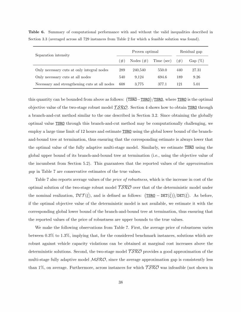
Table 6. Summary of computational performance with and without the valid inequalities described in

Section 3.3 (averaged across all 729 instances from Table 2 for which a feasible solution was found).

Separation intensityProven optimal Residual gap

(#) Nodes (#) Time (sec) (#) Gap (%)

Only necessary cuts at only integral nodes 289 240,540 550.0 440 27.31

Only necessary cuts at all nodes 540 9,124 694.6 189 9.26

Necessary and strengthening cuts at all nodes 608 3,775 377.1 121 5.01

this quantity can be bounded from above as follows:(TSRO−TSRO

)/TSRO, where TSRO is the optimal

objective value of the two-stage robust model T SRO. Section 4 shows how to obtain TSRO through

a branch-and-cut method similar to the one described in Section 3.2. Since obtaining the globally

optimal value TSRO through this branch-and-cut method may be computationally challenging, we

employ a large time limit of 12 hours and estimate TSRO using the global lower bound of the branch-

and-bound tree at termination, thus ensuring that the corresponding estimate is always lower that

the optimal value of the fully adaptive multi-stage model. Similarly, we estimate TSRO using the

global upper bound of its branch-and-bound tree at termination (i.e., using the objective value of

the incumbent from Section 5.2). This guarantees that the reported values of the approximation

gap in Table 7 are conservative estimates of the true values.

Table 7 also reports average values of the price of robustness, which is the increase in cost of the

optimal solution of the two-stage robust model T SRO over that of the deterministic model under

the nominal realization, DET (ξ), and is defined as follows:(TSRO − DET(ξ)

)/DET(ξ). As before,

if the optimal objective value of the deterministic model is not available, we estimate it with the

corresponding global lower bound of the branch-and-bound tree at termination, thus ensuring that

the reported values of the price of robustness are upper bounds to the true values.

We make the following observations from Table 7. First, the average price of robustness varies

between 0.3% to 1.3%, implying that, for the considered benchmark instances, solutions which are

robust against vehicle capacity violations can be obtained at marginal cost increases above the

deterministic solutions. Second, the two-stage model T SRO provides a good approximation of the

multi-stage fully adaptive model MSRO, since the average approximation gap is consistently less

than 1%, on average. Furthermore, across instances for which T SRO was infeasible (not shown in

38

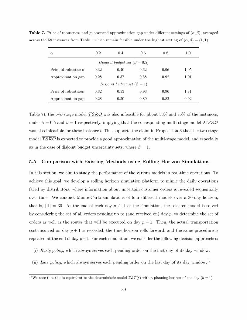
Table 7. Price of robustness and guaranteed approximation gap under different settings of (α, β), averaged

across the 58 instances from Table 1 which remain feasible under the highest setting of (α, β) = (1, 1).

α 0.2 0.4 0.6 0.8 1.0

General budget set (β = 0.5)

Price of robustness 0.32 0.40 0.62 0.96 1.05

Approximation gap 0.28 0.37 0.58 0.92 1.01

Disjoint budget set (β = 1)

Price of robustness 0.32 0.53 0.93 0.96 1.31

Approximation gap 0.28 0.50 0.89 0.82 0.92

Table 7), the two-stage model T SRO was also infeasible for about 53% and 85% of the instances,

under β = 0.5 and β = 1 respectively, implying that the corresponding multi-stage model MSRO

was also infeasible for these instances. This supports the claim in Proposition 3 that the two-stage

model T SRO is expected to provide a good approximation of the multi-stage model, and especially

so in the case of disjoint budget uncertainty sets, where β = 1.

5.5 Comparison with Existing Methods using Rolling Horizon Simulations

In this section, we aim to study the performance of the various models in real-time operations. To

achieve this goal, we develop a rolling horizon simulation platform to mimic the daily operations

faced by distributors, where information about uncertain customer orders is revealed sequentially

over time. We conduct Monte-Carlo simulations of four different models over a 30-day horizon,

that is, |Π| = 30. At the end of each day p ∈ Π of the simulation, the selected model is solved

by considering the set of all orders pending up to (and received on) day p, to determine the set of

orders as well as the routes that will be executed on day p + 1. Then, the actual transportation

cost incurred on day p + 1 is recorded, the time horizon rolls forward, and the same procedure is

repeated at the end of day p+1. For each simulation, we consider the following decision approaches:

(i) Early policy, which always serves each pending order on the first day of its day window,

(ii) Late policy, which always serves each pending order on the last day of its day window,12

12We note that this is equivalent to the deterministic model DET (ξ) with a planning horizon of one day (h = 1).

39

(iii) Deterministic model DET (ξ) with a five-day planning horizon (h = 5), and

(iv) Robust model T SRO with a five-day planning horizon (h = 5) and budgeted uncertainty set.

In the case of the deterministic and robust models, the planning horizon shrinks in the last five days

of the simulation. We note that the early and late policies are very popular in industry because of

their simplicity, and they resemble current industrial practices. Hence, it is natural to benchmark

our proposed method against these approaches.

Each of the above decision-making models ignores information beyond its current planning

horizon. Therefore, it is possible that the selected model can become infeasible on some day of

the simulation, as the fleet size and vehicle capacities are limited. To monetize infeasibility in such

cases, we consider a per-unit penalty cost M of commissioning additional vehicles and solve the

following penalized model to recover implementable routes:

minimizeS,θ

∑p∈P

CVRP(Sp, ξ,m+ θp) +M∑p∈P

θp

subject to (S1, . . . , Sh) ∈ F , θ ∈ Zp+

BPP(Sp, ξ) ≤ m+ θp ∀ p ∈ P, ∀ ξ ∈ Ξ,

Here, θp is a slack variable representing the number of additional vehicles required on day p ∈ P .

In practice, M is typically very large and hence, we can equivalently solve the penalized model

by lexicographically minimizing the number of additional vehicles first, and then minimizing the

vehicle routing cost. Specifically, in the first phase, we determine the minimum total number of

additional vehicles that need to be commissioned, Θ?, by solving the above model without the

routing-related CVRP terms in the objective function. In the second phase, we solve the same model

by setting M = 0, but with an additional constraint on the total number of additional vehicles that

can be used,∑

p∈P θp ≤ Θ?. In the simulation, the final cost recorded is the sum of the routing cost

on day 1, CVRP(S1, ξ,m + θ1), and the incurred penalty cost Mθ1 associated with commissioning

θ1 additional vehicles. We note that, in the above optimization model, F and Ξ are singletons and

P = {1} for the early and late policies, whereas Ξ is a singleton for the deterministic model.

For our simulations, we randomly select 10 instances from Section 5.1 consisting of up to 50

customers, |N | ≤ 50. For each instance, customer orders are simulated as independent Bernoulli

processes with probabilities ∈ {0.25, 0.30, 0.35}, which represent low, medium and high levels of

customer demand. For each combination of test instance, decision-making model and probability

40

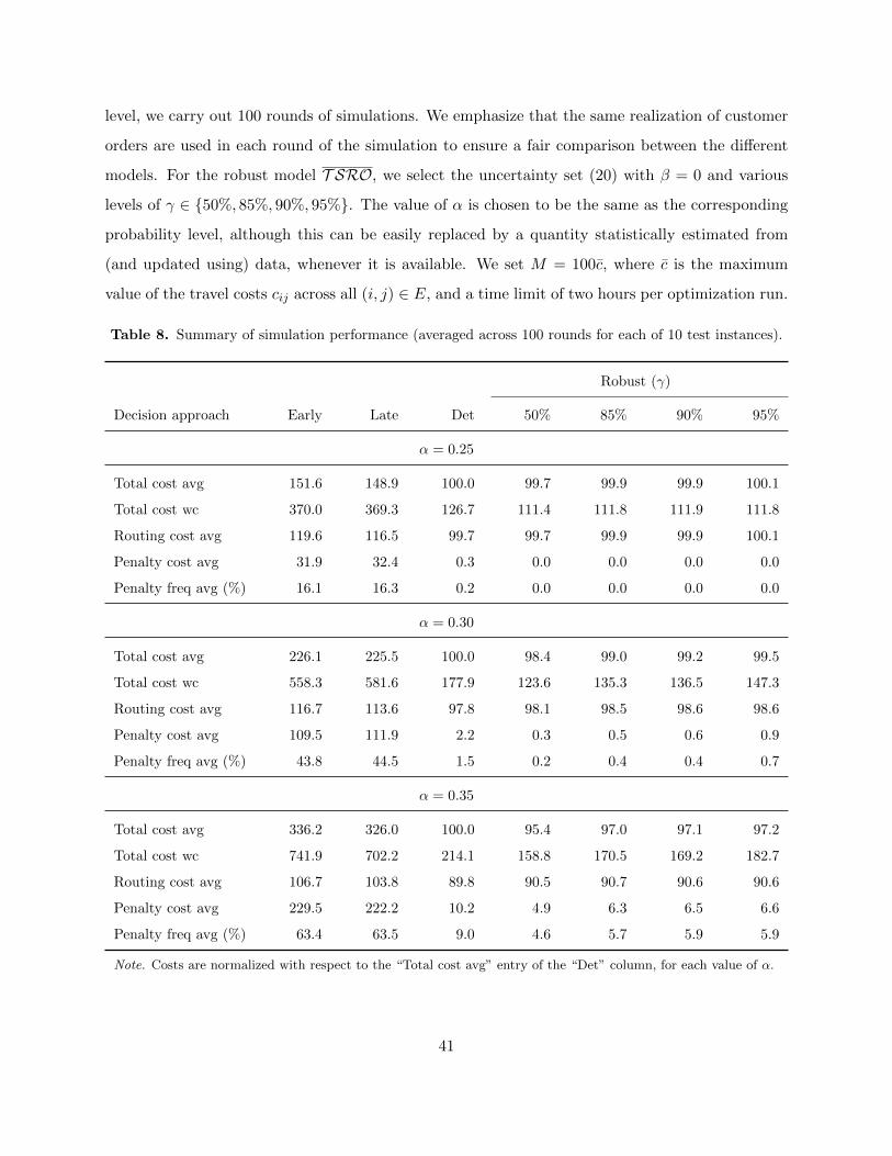
level, we carry out 100 rounds of simulations. We emphasize that the same realization of customer

orders are used in each round of the simulation to ensure a fair comparison between the different

models. For the robust model T SRO, we select the uncertainty set (20) with β = 0 and various

levels of γ ∈ {50%, 85%, 90%, 95%}. The value of α is chosen to be the same as the corresponding

probability level, although this can be easily replaced by a quantity statistically estimated from

(and updated using) data, whenever it is available. We set M = 100c, where c is the maximum

value of the travel costs cij across all (i, j) ∈ E, and a time limit of two hours per optimization run.

Table 8. Summary of simulation performance (averaged across 100 rounds for each of 10 test instances).

Robust (γ)

Decision approach Early Late Det 50% 85% 90% 95%

α = 0.25

Total cost avg 151.6 148.9 100.0 99.7 99.9 99.9 100.1

Total cost wc 370.0 369.3 126.7 111.4 111.8 111.9 111.8

Routing cost avg 119.6 116.5 99.7 99.7 99.9 99.9 100.1

Penalty cost avg 31.9 32.4 0.3 0.0 0.0 0.0 0.0

Penalty freq avg (%) 16.1 16.3 0.2 0.0 0.0 0.0 0.0

α = 0.30

Total cost avg 226.1 225.5 100.0 98.4 99.0 99.2 99.5

Total cost wc 558.3 581.6 177.9 123.6 135.3 136.5 147.3

Routing cost avg 116.7 113.6 97.8 98.1 98.5 98.6 98.6

Penalty cost avg 109.5 111.9 2.2 0.3 0.5 0.6 0.9

Penalty freq avg (%) 43.8 44.5 1.5 0.2 0.4 0.4 0.7

α = 0.35

Total cost avg 336.2 326.0 100.0 95.4 97.0 97.1 97.2

Total cost wc 741.9 702.2 214.1 158.8 170.5 169.2 182.7

Routing cost avg 106.7 103.8 89.8 90.5 90.7 90.6 90.6

Penalty cost avg 229.5 222.2 10.2 4.9 6.3 6.5 6.6

Penalty freq avg (%) 63.4 63.5 9.0 4.6 5.7 5.9 5.9

Note. Costs are normalized with respect to the “Total cost avg” entry of the “Det” column, for each value of α.

41

Table 8 summarizes the simulation performance of the early, late, deterministic (“Det”) and

robust approaches for various ordering levels α. For each approach, each setting of α and each of

the 10 test instances, we compute the average total cost, worst-case total cost, average routing cost

and average penalty cost incurred over the simulation horizon (the average and worst-case being

taken across the 100 simulation rounds), and then normalize each of them with respect to average

total cost incurred by the deterministic model. The average (across the 10 test instances) of these

normalized quantities are then reported in columns Total cost avg, Total cost wc, Routing

cost avg and Penalty cost avg, respectively. The table also reports for each approach and each

setting of α, the percentage of simulations in which penalties were incurred, averaged across the 10

instances, in column Penalty freq avg (%). We make the following observations from Table 8.

1. The early and late policies are strongly outperformed by the deterministic and robust models.

Compared to the latter, they incur about 50% and 220% more cost under the lowest and

highest ordering levels, respectively. This is because they are “myopic”: they ignore not only

uncertain future information, but also existing knowledge of the pending orders (except their

first or last feasible service days). In contrast, the deterministic and robust models “look

ahead” to serve geographically close orders with overlapping day windows in the same route.

2. The robust model at γ = 50% achieves the best overall performance. The outperformance

with respect to the deterministic model is particularly pronounced at higher ordering levels.

Indeed, at α = 0.35, it incurs a total cost which is about 5% lower on average and 26% lower

in the worst-case, and it experiences a 49% lower frequency of infeasibility. Moreover, these

savings come at the price of incurring only 0.9% higher routing costs, on average.

3. Choosing a higher value of γ does not necessarily translate to lower frequencies of infeasibility.

While it is true that a larger uncertainty set leads to a higher probability of being feasible in

a folding horizon context (all else being equal), this is not true in a rolling horizon context.

This is because (i) the models ignore information beyond the current planning horizon, which

is revealed only when time rolls forward, and (ii) on a particular day p > 1, the models

do not necessarily solve the same problem, since their previous decisions lead to different

instantiations of the problem parameters (e.g., the set of pending orders). A similar discussion

can be found in Gorissen et al. [2015] in the context of general robust optimization problems.

42

6 Conclusions

This paper studied the robust multi-period VRP under customer order uncertainty, in which cus-

tomers call-in to request service over a short-term planning horizon, specifying a set of days during

which the service can take place. The decision-maker aims to select a visit schedule over the plan-

ning horizon that remains feasible for all realizations of uncertain customer orders, which were

modeled as binary random variables supported on a finite uncertainty set. The true multi-stage

decision-making process was approximated from above and below by two two-stage robust opti-

mization models. For each approximation, an integer programming formulation was derived and

a numerically efficient branch-and-cut solution technique was presented. Extensive computational

experiments conducted on a number of test instances derived from standard benchmark datasets

showed that robust feasible solutions can be obtained with a computational effort similar to that

for nominal solutions, and that are of high quality, on average. A rolling horizon simulation study

further showed that the robust solutions outperform the nominal solutions in terms of reducing the

frequency of vehicle capacity violations while incurring only marginally higher routing costs.

Acknowledgements

Chrysanthos E. Gounaris and Anirudh Subramanyam gratefully acknowledge support from the U.S.

National Science Foundation (award number CMMI-1434682) and the Center for Advanced Pro-

cess Decision-making at Carnegie Mellon University. Anirudh Subramanyam further acknowledges

support from the John and Claire Bertucci Graduate Fellowship Program. Finally, all authors

gratefully acknowledge the valuable comments from the editors and referees, which have led to a

significantly improved version of this manuscript.

References

A. Agra, M. Christiansen, R. Figueiredo, L. M. Hvattum, M. Poss, and C. Requejo. The robust vehicle routing

problem with time windows. Computers & Operations Research, 40(3):856–866, 2013.

M. Albareda-Sambola, E. Fernandez, and G. Laporte. The dynamic multiperiod vehicle routing problem with prob-

abilistic information. Computers and Operations Research, 48:31–39, 2014.

43

G. Andreatta and G. Lulli. A multi-period TSP with stochastic regular and urgent demands. European Journal of

Operational Research, 185(1):122–132, 2008.

E. Angelelli, M. Grazia Speranza, and M. W. Savelsbergh. Competitive analysis for dynamic multiperiod uncapaci-

tated routing problems. Networks, 49(4):308–317, 2007a.

E. Angelelli, M. W. Savelsbergh, and M. Grazia Speranza. Competitive analysis of a dispatch policy for a dynamic

multi-period routing problem. Operations Research Letters, 35(6):713–721, 2007b.

E. Angelelli, N. Bianchessi, R. Mansini, and M. Speranza. Short Term Strategies for a Dynamic Multi-Period Routing

Problem. Transportation Research Part C: Emerging Technologies, 17(2):106–119, 2009.

C. Archetti, O. Jabali, and M. G. Speranza. Multi-period Vehicle Routing Problem with Due dates. Computers &

Operations Research, 61:122–134, 2015.

T. Athanasopoulos and I. Minis. Multi-period routing in Hybrid Courier Operations. In Supply Chain Optimization,

Design, and Management, pages 232–251. IGI Global, 2011.

T. Athanasopoulos and I. Minis. Efficient techniques for the multi-period vehicle routing problem with time windows

within a branch and price framework. Annals of Operations Research, 206(1):1–22, 2013.

N. Azi, M. Gendreau, and J.-Y. Potvin. A dynamic vehicle routing problem with multiple delivery routes. Annals of

Operations Research, 199(1):103–112, 2012.

E. Balas. Facets of the knapsack polytope. Mathematical Programming, 8(1):146–164, 1975.

R. Baldacci, E. Bartolini, A. Mingozzi, and A. Valletta. An Exact Algorithm for the Period Routing Problem.

Operations Research, 59(1):228–241, 2011.

C. Bandi and D. Bertsimas. Tractable stochastic analysis in high dimensions via robust optimization. Mathematical

programming, 134(1):23–70, 2012.

T. Bekta¸s, P. P. Repoussis, and C. D. Tarantilis. Chapter 11: Dynamic Vehicle Routing Problems. In Vehicle

Routing, pages 299–347. Society for Industrial and Applied Mathematics, Philadelphia, PA, 2014.

A. Ben-Tal, A. Goryashko, E. Guslitzer, and A. Nemirovski. Adjustable robust solutions of uncertain linear programs.

Mathematical Programming, 99(2):351–376, 2004.

A. Ben-Tal, L. El Ghaoui, and A. Nemirovski. Robust Optimization. Princeton Series in Applied Mathematics.

Princeton University Press, 2009.

R. W. Bent and P. Van Hentenryck. Scenario-Based Planning for Partially Dynamic Vehicle Routing with Stochastic

Customers. Operations Research, 52(6):977–987, 2004.

D. Bertsimas. Probabilistic combinatorial optimization problems. PhD thesis, MIT, 1988.

44

D. Bertsimas and C. Caramanis. Finite Adaptability in Multistage Linear Optimization. IEEE Transactions on

Automatic Control, 55(12):2751–2766, 2010.

D. Bertsimas and I. Dunning. Multistage Robust Mixed-Integer Optimization with Adaptive Partitions. Operations

Research, 64(4):980–998, 2016.

D. Bertsimas and A. Georghiou. Binary Decision Rules for Multistage Adaptive Mixed-Integer Optimization. Available

on Optimization Online, 2014.

D. Bertsimas and A. Georghiou. Design of Near Optimal Decision Rules in Multistage Adaptive Mixed-Integer

Optimization. Operations Research, 63(3):610–627, 2015.

D. Bertsimas and M. Sim. The Price of robustness. Operations Research, 52(1):35–53, 2004.

D. Bertsimas, D. B. Brown, and C. Caramanis. Theory and Applications of Robust Optimization. SIAM Review, 53

(3):464–501, 2011.

D. Bertsimas, S. Gupta, and J. Tay. Scalable Robust and Adaptive Inventory Routing. Available on Optimization

Online, 2016.

D. Bertsimas, V. Gupta, and N. Kallus. Data-driven robust optimization. Mathematical Programming, 167(2):

235–292, 2018.

J. R. Birge and F. Louveaux. Introduction to Stochastic Programming. Springer Series in Operations Research and

Financial Engineering. Springer New York, New York, NY, 2011.

N. Bostel, P. Dejax, P. Guez, and F. Tricoire. Multiperiod planning and routing on a rolling horizon for field force

optimization logistics. In B. Golden, S. Raghavan, and E. Wasil, editors, The Vehicle Routing Problem: Latest

Advances and New Challenges, pages 503–525. Springer US, Boston, MA, 2008.

L. Chen, M. Gendreau, M. H. Ha, and A. Langevin. A robust optimization approach for the road network daily main-

tenance routing problem with uncertain service time. Transportation Research Part E: Logistics and Transportation

Review, 85:40–51, 2016.

X. Chen and Y. Zhang. Uncertain Linear Programs: Extended Affinely Adjustable Robust Counterparts. Operations

Research, 57(6):1469–1482, 2009.

J.-F. Cordeau, M. Dell’Amico, S. Falavigna, and M. Iori. A rolling horizon algorithm for auto-carrier transportation.

Transportation Research Part B: Methodological, 76:68–80, 2015.

I. Dayarian, T. G. Crainic, M. Gendreau, and W. Rei. A branch-and-price approach for a multi-period vehicle routing

problem. Computers & Operations Research, 55:167–184, 2015.

45

S. T. DeNegre and T. K. Ralphs. A Branch-and-cut Algorithm for Integer Bilevel Linear Programs. In J. W. Chinneck,

B. Kristjansson, and M. J. Saltzman, editors, Operations Research and Cyber-Infrastructure, pages 65–78. Springer

US, Boston, MA, 2009.

A. L. Erera, J. C. Morales, and M. Savelsbergh. The Vehicle Routing Problem with Stochastic Demand and Duration

Constraints. Transportation Science, 44(4):474–492, 2010.

M. Fischetti, J. J. S. Gonzalez, and P. Toth. Solving the Orienteering Problem through Branch-and-Cut. INFORMS

Journal on Computing, 10(2):133–148, 1998.

P. M. Francis, K. R. Smilowitz, and M. Tzur. The period vehicle routing problem and its extensions. In B. Golden,

S. Raghavan, and E. Wasil, editors, The Vehicle Routing Problem: Latest Advances and New Challenges, pages

73–102. Springer US, Boston, MA, 2008.

M. Gendreau, G. Laporte, and R. Seguin. An Exact Algorithm for the Vehicle Routing Problem with Stochastic

Demands and Customers. Transportation Science, 29(2):143–155, 1995.

M. Gendreau, G. Laporte, and F. Semet. Heuristics and lower bounds for the bin packing problem with conflicts.

Computers & Operations Research, 31(3):347–358, 2004.

M. Gendreau, O. Jabali, and W. Rei. Chapter 8: Stochastic Vehicle Routing Problems. In P. Toth and D. Vigo,

editors, Vehicle Routing, volume 18, pages 213–239. Society for Industrial and Applied Mathematics, Philadelphia,

PA, 2014.

B. Golden, S. Raghavan, and E. Wasil. The Vehicle Routing Problem: Latest Advances and New Challenges. Opera-

tions Research/Computer Science Interfaces. Springer US, Boston, MA, 2008.

B. L. Gorissen, I. Yanıkoglu, and D. den Hertog. A practical guide to robust optimization. Omega, 53:124–137, 2015.

C. E. Gounaris, W. Wiesemann, and C. A. Floudas. The Robust Capacitated Vehicle Routing Problem Under

Demand Uncertainty. Operations Research, 61(3):677–693, 2013.

C. E. Gounaris, P. P. Repoussis, C. D. Tarantilis, W. Wiesemann, and C. A. Floudas. An Adaptive Memory

Programming Framework for the Robust Capacitated Vehicle Routing Problem. Transportation Science, 50(4):

1239–1260, 2016.

G. A. Hanasusanto, D. Kuhn, and W. Wiesemann. K -Adaptability in Two-Stage Robust Binary Programming.

Operations Research, 63(4):877–891, 2015.

V. Hemmelmayr, K. F. Doerner, R. F. Hartl, and M. W. P. Savelsbergh. Delivery strategies for blood products

supplies. OR Spectrum, 31(4):707–725, 2009.

S. Irnich, M. Schneider, and D. Vigo. Chapter 9: Four Variants of the Vehicle Routing Problem. In Vehicle Routing,

pages 241–271. Society for Industrial and Applied Mathematics, Philadelphia, PA, 2014.

46

P. Jaillet. A Priori Solution of a Traveling Salesman Problem in Which a Random Subset of the Customers Are

Visited. Operations Research, 36(6):929–936, 1988.

P. Jaillet, J. Qi, and M. Sim. Routing Optimization Under Uncertainty. Operations Research, 64(1):186–200, 2016.

K. Jansen and S. Ohring. Approximation Algorithms for Time Constrained Scheduling. Information and Computation,

132(2):85–108, 1997.

M. A. Klapp, A. L. Erera, and A. Toriello. The Dynamic Dispatch Waves Problem for Same-Day Delivery. Available

on Optimization Online, 2016.

G. Laporte, F. V. Louveaux, and H. Mercure. A Priori Optimization of the Probabilistic Traveling Salesman Problem.

Operations Research, 42(3):543–549, 1994.

A. Larsen, O. Madsen, and M. Solomon. Partially dynamic vehicle routing—models and algorithms. Journal of the

Operational Research Society, 53(6):637–646, 2002.

J. Lysgaard, A. N. Letchford, and R. W. Eglese. A new branch-and-cut algorithm for the capacitated vehicle routing

problem. Mathematical Programming, 100(2):423–445, 2004.

S. Martello and P. Toth. Knapsack Problems: Algorithms and Computer Implementations. John Wiley & Sons, Inc.,

New York, NY, USA, 1990.

S. T. McCormick, M. Rao, and G. Rinaldi. Easy and difficult objective functions for max cut. Mathematical

Programming, 94(2-3):459–466, 2003.

F. Ordonez. Robust Vehicle Routing. In J. J. Hasenbein, editor, INFORMS TutORials in Operations Research,

chapter 7, pages 153–178. INFORMS, Hanover MD, 2010.

K. Postek and D. den Hertog. Multistage Adjustable Robust Mixed-Integer Optimization via Iterative Splitting of

the Uncertainty Set. INFORMS Journal on Computing, 28(3):553–574, 2016.

N. Secomandi and F. Margot. Reoptimization Approaches for the Vehicle-Routing Problem with Stochastic Demands.

Operations Research, 57(1):214–230, 2009.

O. Solyalı, J.-F. Cordeau, and G. Laporte. Robust Inventory Routing Under Demand Uncertainty. Transportation

Science, 46(3):327–340, 2012.

I. Sungur, F. Ordonez, and M. Dessouky. A robust optimization approach for the capacitated vehicle routing problem

with demand uncertainty. IIE Transactions, 40(5):509–523, 2008.

H. Tang, E. Miller-Hooks, and R. Tomastik. Scheduling technicians for planned maintenance of geographically

distributed equipment. Transportation Research Part E: Logistics and Transportation Review, 43(5):591–609,

2007.

47

Y. Tang, J.-P. P. Richard, and J. C. Smith. A class of algorithms for mixed-integer bilevel min–max optimization.

Journal of Global Optimization, 66(2):225–262, 2016.

P. Toth and D. Vigo. Vehicle Routing: Problems, Methods, and Applications, Second Edition. MOS-SIAM Series on

Optimization. Society for Industrial and Applied Mathematics, Philadelphia, PA, USA, 2014.

F. Tricoire. Vehicle and personnel routing optimization in the service sector: application to water distribution and

treatment. 4OR, 5(2):165–168, 2007.

M. W. Ulmer, D. C. Mattfeld, and N. Soeffker. Dynamic multi-period vehicle routing: approximate value iteration

based on dynamic lookup tables. Available online, 2016. URL http://web.winforms.phil.tu-bs.de/paper/

ulmer/WP_Ulmer_Dynamic_Lookup.pdf.

M. Wen, J.-F. Cordeau, G. Laporte, and J. Larsen. The dynamic multi-period vehicle routing problem. Computers

& Operations Research, 37(9):1615–1623, 2010.

B. Zeng and Y. An. Solving Bilevel Mixed Integer Program by Reformulations and Decomposition. Available on

Optimization Online, 2014.

Y. Zhang, R. Baldacci, M. Sim, and J. Tang. Routing optimization with time windows under uncertainty. Mathe-

matical Programming, 2018.

L. Zhao and B. Zeng. An Exact Algorithm for Two-stage Robust Optimization with Mixed Integer Recourse Problems.

Available on Optimization Online, 2012.

48

A Proofs of Propositions

Proof of Proposition 1. The first inequality follows from the observation that T SRO is equivalent

to the following problem:

minimizeS,R

∑p∈P

CVRP(Sp, ξ,m)

subject to (S1, S2, . . . , Sh) ∈ F

BPP(Sp, ξ) ≤ m ∀ p ∈ P \ {1}

Rp : Ξ \ {ξ} 7→ 2∆p ∀ p ∈ P \ {1}

(S1, R2(ξ), . . . , Rh(ξ)) ∈ F ∀ ξ ∈ Ξ \ {ξ}

BPP(Rp(ξ), ξ) ≤ m ∀ p ∈ P \ {1}, ∀ ξ ∈ Ξ \ {ξ}

This description differs from the original one in that it has explicit decision variables for the

assignments resulting from evaluating the functionals Sp(·) under the nominal scenario. Observe

that the second constraint in the above problem is redundant since it is embedded in the evaluation

of CVRP(Sp, ξ,m) in the objective function. Therefore, DET (ξ) is obtained by relaxing the last

three constraints and its optimal value provides a lower bound to that of T SRO.

The second inequality follows from the fact that for any feasible solution (S1, S2(·), . . . , Sh(·))

inMSRO, we can construct a feasible solution (S′1, S′2(·), . . . , S′h(·)) in T SRO as follows: S′1 = S1

and S′p(ξ) , Sp(ξ[p−1]) for all ξ ∈ Ξ. Therefore, the feasible region of MSRO is a subset of the

feasible region of T SRO and its optimal value provides an upper bound to that of T SRO.

The third inequality follows if, for all p > 1, we restrict the functional variables Sp(·) inMSRO

to the space of constant functions. In doing so, we obtain T SRO, whose optimal value provides

an upper bound to the optimal value of MSRO.

Proof of Proposition 2. In either case, the optimal functions Sp(·), for all p ∈ P \ {1}, in both

models T SRO andMSRO can be obtained as follows: Sp(·) ≡ {v ∈ V : p ∈ Pv, v /∈ S1}, i.e., they

are constant over their domain. Therefore, the functional variables Sp : Ξ 7→ 2∆p in T SRO and

Sp : Ξ[p−1] 7→ 2∆p in MSRO can be replaced with the decision variables Sp ∈ 2∆p (i.e., Sp ⊆ ∆p)

without loss of optimality. In both cases, the model obtained by restricting the functional variables

to the space of constant functions is optimal and, therefore, equivalent to T SRO.

49

Proof of Proposition 3. The stated result clearly holds under conditions of Proposition 2 for which

MSRO = TSRO.

Consider now case (i). Assume that (S1, S2(·), . . . , Sh(·)) is a feasible solution in modelMSRO.

Consider the order assignment S = (S1, S2(1[1]), . . . , Sh(1[h−1])) obtained by evaluating this feasible

solution under the worst-case uncertainty realization, 1 ∈ Ξ, where Ξ is a hypercube. This assign-

ment is also feasible in model T SRO since (a) S ∈ F , as per the second constraint in MSRO,

and (b) BPP(Sp(1[p−1]), ξ) ≤ BPP(Sp(1

[p−1]),1) ≤ m is satisfied for all ξ ∈ Ξ; indeed, the second

inequality follows from the third constraint in model MSRO, while the first inequality follows

from the fact that the optimal value of the bin-packing problem associated with any set is always

no larger than the optimal value associated with any subset.

Consider now case (ii). Define ξ = (ξ0, ξ1, . . . , ξh−1) ∈ Ξ as follows: ξp := (ξv[p])v∈Vp , where

ξ[p] is an optimal solution of maxξ∈Ξ BPP(Sp, ξ), where Sp := {v ∈ V : Pv = {p}} for all p ∈ P \{1}.

Similar to case (ii), assume that (R1, R2(·), . . . , Rh(·)) is a feasible solution in model MSRO.

Now, consider the R = (R1, R2(ξ[1]), . . . , Rh(ξ[h−1])) to be the order assignment obtained by eval-

uating this feasible solution under the uncertainty realization ξ ∈ Ξ. This assignment is also

feasible in model T SRO since (a) R ∈ F , as per the second constraint in MSRO, and (b)

BPP(Rp(ξ[p−1]), ξ) ≤ BPP(Rp(ξ

[p−1]), ξ) ≤ m for all ξ ∈ Ξ; indeed, the second inequality follows

from the third constraint in MSRO, while the first inequality follows from the fact that ξ is an

optimal solution of maxξ∈Ξ BPP(Rp(ξ[p−1]), ξ). We remark that the latter holds because the proof of

Proposition 7 shows that this optimal value only depends on orders in Rp(ξ[p−1])

⋂q∈P,l Clq = Sp.

In turn, this last equality holds because all customers i ∈ N with wi ≥ 2 satisfy (i, q) /∈ Clq for any

l, q (since all orders from i are preprocessed from the uncertainty set, i.e., (i, q) /∈ V for any q ∈ P ),

and any customer order v = (i, q) with wi = 1 and q 6= p − 1 satisfies v /∈ Rp(ξ[p−1]) (since ei = 1

for all such orders).

Proof of Proposition 4. Necessity. Let S(y) be any robust feasible solution in T SRO that is in-

duced by binary variables y. Also, let S ⊆ V , p ∈ P and ξ ∈ Ξ be given. Then we have that:

m+∑i∈S

(1− yip) = m+∑

i∈S∩Sp(y)

(1− 1) +∑

i∈S\Sp(y)

(1− 0)

= m+ |S \ Sp(y)|

≥ BPP(Sp(y), ξ) + |S \ Sp(y)|

50

≥ BPP(S ∩ Sp(y), ξ) + |S \ Sp(y)|

≥ BPP(S ∩ Sp(y), ξ) + BPP(S \ Sp(y), ξ)

≥ BPP(S, ξ)

Here, the first equality follows from (8). The first inequality follows from the definition of robust

feasibility of S(y) in T SRO. The second inequality follows from the fact that the optimal value

of the bin packing problem over a given set of items is always no smaller than its optimal value

over any subset of items. The third inequality follows from the fact that the cardinality of the set

of items is a trivial upper bound to the optimal value of the corresponding bin packing problem.

Finally, the last inequality follows from the fact that the optimal value of the bin packing problem

possesses the subadditivity property.

Sufficiency. Assume that y satisfies equations (9) and the robust cover inequalities (11). We

must then show that S(y) is a robust feasible solution in T SRO. From equations (8)–(9), we know

that S(y) partitions V ; that is, S(y) ∈ F . We therefore only need to verify that, for every ξ ∈ Ξ

and p ∈ P , the relationship BPP(Sp(y), ξ) ≤ m holds. This is true since the left-hand side of (11)

for S = Sp(y) evaluates to m, whereas the right-hand side evaluates to BPP(Sp(y), ξ).

Proof of Proposition 5. Instead of proving the proposition directly, we prove its contra-position:

if inequality (12) associated with p ∈ P is violated by some solution (x∗, y∗) of the constraint

system (10b)–(10h), then at least one of the robust cover inequalities (11) associated with p is also

violated by (x∗, y∗). Therefore, let us assume that∑

i∈S ξi(1− y∗ip)−∑

i∈N(S) ξiy∗ip < k is satisfied.

Consider the robust cover inequality (11) defined by period p, customer order realization ξ, and

the subset S′ = S+ ∪NS+, where S+ = {i ∈ S ∩ Sp(y∗) : ξi = 1} and NS+ = {i ∈ N(S)∩ Sp(y∗) :

ξi = 1}. We shall prove that this inequality is violated by (x∗, y∗). Observe that the left-hand

side of this inequality evaluates to m since i ∈ Sp(y∗) is satisfied for all i ∈ S′ by construction.

Therefore, we would like to show that its right-hand side exceeds m; that is, BPP(S′, ξ) ≥ m+ 1.

We define the set S1 = {i ∈ S : ξi = 1} for ease of notation. Note that BPP(S1, ξ) = BPP(S, ξ) ≥

m+ k, where k ≥ 1, holds by hypothesis. We now consider two different cases:

(i) |S+| >∣∣S1∣∣− k.

Observe that, since S+ ⊆ S1 and |S+| >∣∣S1∣∣− k, S+ is obtained from S1 after the removal

of fewer than k elements. Therefore, the optimal bin packing value associated with S+ can

51

only decrease by some number less than k with respect to the optimal bin packing value

associated with S1; that is, BPP(S+, ξ) ≥ BPP(S1, ξ) − (k − 1) ≥ m + k − (k − 1) = m + 1.

Since BPP(S′, ξ) ≥ BPP(S+, ξ), we have that BPP(S′, ξ) ≥ m+ 1.

(ii) |S+| ≤∣∣S1∣∣− k.

Let S− be any non-empty subset of S1 \ S+ such that |S−| =∣∣S1∣∣ − |S+| − (k − 1). It is

possible to construct such a subset since |S+| ≤∣∣S1∣∣− k and k ≥ 1. The following holds:

BPP(S′, ξ) = BPP(S+ ∪NS+, ξ)

≥ BPP(S+ ∪ S−, ξ)

≥ BPP(S1, ξ)− (k − 1)

≥ m+ 1

The first inequality follows from the following two observations: (i) our hypothesis is∑

i∈S ξi(1−

y∗ip)−∑

i∈N(S) ξiy∗ip < k; this is equivalent to |NS+| >

∣∣S1∣∣− |S+| − k = |S−|, and (ii) each

item of NS+ has higher weight (i.e., demand) than each item of S− since NS+ ⊆ N(S). The

second inequality follows from the fact that S+ ∪ S− ⊆ S1 and S+ ∪ S− is constructed from

S1 by the removal of k − 1 customers. Therefore, the optimal bin packing value associated

with S+∪S− can only decrease by at most k−1 with respect to the optimal value associated

with S1. The last inequality follows from BPP(S1, ξ) ≥ m+ k, where k ≥ 1.

Proof of Proposition 6. Consider the following relaxation of formulation (10) obtained by relaxing

the day window constraints (10e) and the fleet availability constraints (10f):

(10)′ minimizex,y

∑p∈P

∑v∈V0

c0vx0vp +∑p∈P

∑(u,v)∈E0

cuvxuvp

subject to yvp ∈ {0, 1} ∀ v ∈ V, ∀ p ∈ P

x0vp ∈ {0, 1, 2} ∀ v ∈ V0, ∀ p ∈ P

xuvp ∈ {0, 1} ∀ (u, v) ∈ E0, ∀ p ∈ P∑p∈P

yvp = 1 ∀ v ∈ V0

52

x0vp +∑

u:(u,v)∈E0

xuvp = 2yvp ∀ v ∈ V0, ∀ p ∈ P

∑p∈P

∑(u,v)∈E0(S)

xuvp ≤ |S| −

⌈1

Q

∑i∈S

qi

⌉∀ S ⊆ V0

Now, if we add the two-index variables to the above formulation, via the identities x′uv =∑

p∈P xuvp

for all (u, v) ∈ E0∪{(0, v′) : v′ ∈ V0}, and project the resulting integer polytope into the space of the

two-index variables x′, we obtain the integer polytope associated with the following formulation:

minimizex′

∑v∈V0

c0vx′0v +

∑(u,v)∈E0

cuvx′uv

subject to x′0v ∈ {0, 1, 2} ∀ v ∈ V0

x′uv ∈ {0, 1} ∀ (u, v) ∈ E0

x0v +∑

u:(u,v)∈E0

xuv = 2 ∀ v ∈ V0

∑(u,v)∈E0(S)

xuv ≤ |S| −

⌈1

Q

∑i∈S

qi

⌉∀ S ⊆ V0

This is precisely the two-index formulation of the CVRP instance defined on the subgraph of G with

depot node 0, customers V0, edges E0, demands qv for v ∈ V0 and vehicle capacity Q. Therefore,

if∑

(i,j)∈I λijx′ij ≤ µ is any valid inequality for the above two-index formulation, the inequality∑

p∈P∑

(i,j)∈I λijxijp ≤ µ is valid for formulation (10)′ and, hence, valid for formulation (10), since

the former constitutes a relaxation of the latter.

Proof of Proposition 7. We consider values of ξ∗v , v ∈ V , for each of the following cases separately:

1. v /∈ (V0 ∪ S).

Observe that, for given ξ ∈ Ξ, we can set ξv = 0 without changing the value of BPP(S, ξ) and

without affecting the validity of ξ ∈ Ξ (since each budget constraint continues to be satisfied).

Therefore, there always exists an optimal solution that satisfies ξv = 0 for all v /∈ (V0 ∪ S).

2. v ∈ (V0 ∪ S) \(∪Ll=1Bl

). This is equivalent to v ∈ J0, by construction.

Observe that, if ξv = 0, then setting ξv = 1 does not decrease the value of BPP(S, ξ) and,

moreover, we do not violate ξ ∈ Ξ (since ξv does not appear in any budget constraint).

Therefore, any maximizer ξ∗ of BPP(S, ξ) must also satisfy ξ∗v = 1 for all v ∈ J0.

53

3. v ∈ (V0 ∪ S) ∩(∪Ll=1Bl

). This is equivalent to v ∈ S ∩

(∪Ll=1Bl

)since, by construction, we

have V0 ∩(∪Ll=1Bl

)= ∅.

Since the subsets {Bl}Ll=1 are disjoint by assumption, assume that v ∈ S∩Bl, where 1 ≤ l ≤ L

is some budget, and that v /∈ Bl′ , for all l′ 6= l. There are two possibilities:

(i) If |S ∩Bl| ≤ bl, or if |S ∩Bl| > bl and v = vl,j for some j ≤ bl, then we can set ξ∗v = 1,

since doing so does not violate any budget constraint (i.e., ξ∗ ∈ Ξ is satisfied) and does not

decrease the value of BPP(S, ξ∗).

(ii) If |S ∩Bl| > bl and v = vl,j for some j > bl, then we must have ξ∗v = 0. Indeed, if

ξ∗v = 1, and since ξ∗ ∈ Ξ, i.e.,∑

v′∈Blξ∗v′ ≤ bl, then there exists k ∈ {vl,1, . . . , vl,bl} such that

ξ∗k = 0. In this case, one can obtain a potentially higher bin packing value associated with the

realization obtained by setting ξ∗v = 0 and ξ∗k = 1 (since k has a higher demand with respect

to v), contradicting the fact that ξ∗ is a maximizer of BPP(S, ξ).

We remark that, with a slight modification, this proof can also be used to show the correctness of the

separation procedure for the robust cumulative capacity inequalities outlined in Section 3.4.2.

Proof of Proposition 8. The proof is almost identical to that of Proposition 4. Nevertheless, we

present it for the sake of completeness.

Necessity. Let S1(y) be any customer order assignment on day 1 such that the existence of a fea-

sible solution (S1(y), S2(·), . . . , Sh(·)) in T SRO is guaranteed. Also, let S ⊆ V \{v ∈ V : Pv = {1}}

and ξ ∈ Ξ be given. Then, we have that:

m(h− 1) +∑i∈S

yi1 = m(h− 1) +∑i∈S

I[i∈S1(y)]

= m(h− 1) + |S ∩ S1(y)|

≥ BPPDW(V \ S1(y), ξ) + |S ∩ S1(y)|

≥ BPPDW(S \ S1(y), ξ) + |S ∩ S1(y)|

≥ BPPDW(S, ξ)

The first equality follows from (17) and the fact that the assignment, S1(y), is common for realiza-

tions ξ and ξ. The first inequality follows from the following two observations: (i) by definition,

the customer order assignment (S1(y), S2(ξ), . . . , Sh(ξ)) is such that each subset Sp(ξ) for p > 1 can

be partitioned into m capacity-feasible routes, say (rp,1, . . . , rp,m) and (ii) (S1(y), S2(ξ), . . . , Sh(ξ))

54

partitions V . Therefore, the feasible space of the corresponding bin packing problem with day win-

dows defined over the set of items V \S1(y), under realization ξ, contains the partition r2,1, . . . , r2,m,

. . ., rh,1, . . . , rh,m. Hence, m(h−1) constitutes an upper bound to its optimal value, resulting in the

first inequality. The second inequality follows from the fact that S ⊆ V and that the optimal value

of the bin packing problem with day windows over a given set of items is always no smaller than

its optimal value over any subset of items. The third inequality follows from the fact that if the set

of items is enlarged by an additional item, then the optimal value of the bin packing problem can

increase by at most one.

Sufficiency. Assume that y satisfies equations (9) and the robust cover inequalities (18). We

must show that the customer order assignment on day 1, S1(y), is such that there exists a feasible

solution (S1(y), S2(·), . . . , Sh(·)) in T SRO. Let ξ ∈ Ξ be any customer order realization. We shall

construct the feasible solution as follows. By hypothesis, for S = V \ S1(y) and customer order

realization ξ, the robust cover inequality (18) is satisfied. The left-hand side of this inequality

evaluates to m(h− 1), whereas the right-hand side is the optimal value of the bin packing problem

with day windows defined over the set of items V \ S1(y) with weights qiξi, day windows Pi \ {1},

and set of days P \{1} and bin capacity Q. This implies that there is a capacity-feasible partition of

the items, say (r2,1, . . . , r2,m, . . . , rh,1, . . . , rh,m). Therefore, for each p ∈ P \{1}, we construct Sp(ξ)

according to Sp(ξ) =⋃k∈K

rp,k. By construction and from (9), (S1(y), S2(ξ), . . . , Sh(ξ)) partitions V

and is capacity-feasible under realization ξ.

B Example Illustrating the Decision Dynamics of the Determin-

istic and Two-Stage Robust Optimization Models

Consider the instance shown in Figure 1 with n = 6 customers and m = 1 vehicle of capacity Q = 4.

Note that, for the sake of simplicity, every order from a given customer i ∈ N always has the same

demand qi and day windows {d+ ei, . . . , d+ `i} (assuming the order was placed on day d).

Suppose that the set of pending orders at the end of the current day, i.e., day 0 ∈ Π, is

V0 = {(1,−3), (2,−1), (3, 0), (4,−2)}; that is, customers 1, 2 and 4 have respectively placed orders

on days −3, −1 and −2 that are still pending, while customer 3 has just placed an order on day 0.

There are currently no pending orders from customers 5 and 6. Suppose that there are h = 4 days

55

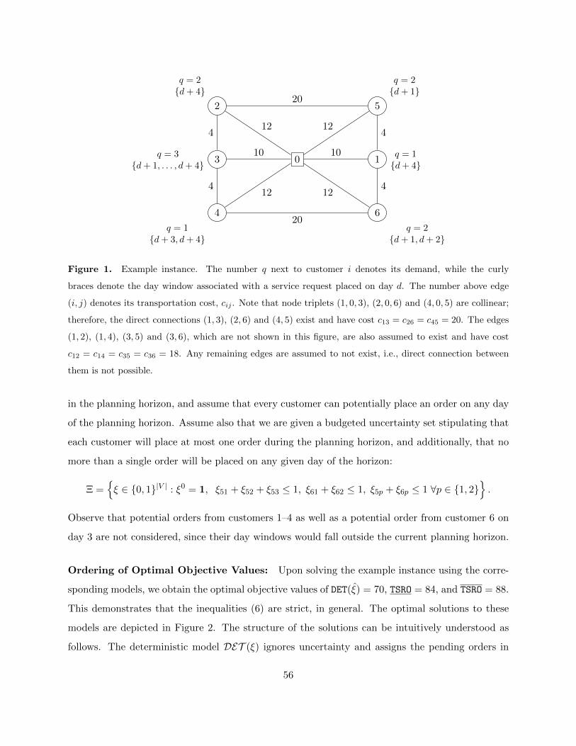
0 1

2

3

4

5

6

4

4

10

12

12

10

12

12

4

4

20

20

q = 2{d+ 4}

q = 3{d+ 1, . . . , d+ 4}

q = 1{d+ 3, d+ 4}

q = 1{d+ 4}

q = 2{d+ 1}

q = 2{d+ 1, d+ 2}

Figure 1. Example instance. The number q next to customer i denotes its demand, while the curly

braces denote the day window associated with a service request placed on day d. The number above edge

(i, j) denotes its transportation cost, cij . Note that node triplets (1, 0, 3), (2, 0, 6) and (4, 0, 5) are collinear;

therefore, the direct connections (1, 3), (2, 6) and (4, 5) exist and have cost c13 = c26 = c45 = 20. The edges

(1, 2), (1, 4), (3, 5) and (3, 6), which are not shown in this figure, are also assumed to exist and have cost

c12 = c14 = c35 = c36 = 18. Any remaining edges are assumed to not exist, i.e., direct connection between

them is not possible.

in the planning horizon, and assume that every customer can potentially place an order on any day

of the planning horizon. Assume also that we are given a budgeted uncertainty set stipulating that

each customer will place at most one order during the planning horizon, and additionally, that no

more than a single order will be placed on any given day of the horizon:

Ξ ={ξ ∈ {0, 1}|V | : ξ0 = 1, ξ51 + ξ52 + ξ53 ≤ 1, ξ61 + ξ62 ≤ 1, ξ5p + ξ6p ≤ 1 ∀p ∈ {1, 2}

}.

Observe that potential orders from customers 1–4 as well as a potential order from customer 6 on

day 3 are not considered, since their day windows would fall outside the current planning horizon.

Ordering of Optimal Objective Values: Upon solving the example instance using the corre-

sponding models, we obtain the optimal objective values of DET(ξ) = 70, TSRO = 84, and TSRO = 88.

This demonstrates that the inequalities (6) are strict, in general. The optimal solutions to these

models are depicted in Figure 2. The structure of the solutions can be intuitively understood as

follows. The deterministic model DET (ξ) ignores uncertainty and assigns the pending orders in

56

a way that optimizes the cost of routing them; only 1 unit of demand is served on day 1. The

two-stage model T SRO considers uncertainty (albeit in an anticipative manner) and serves 2 units

of demand on day 1; this frees up some of the vehicle capacity in future time periods, but incurs

higher routing cost. The non-anticipative two-stage model T SRO frees up even more of the vehicle

capacity in future time periods, serving 3 units of demand on day 1, but incurs the highest routing

cost.

0 1

2

3

4

Day 1

Day 3

Day 2

0 1

2

3

4

Day 1

Day 2

Day 3

0 1

2

3

4

Day 3

Day 1

Day 2

Figure 2. From left to right, the graphs illustrate the optimal routes passing through the set of pending

orders, corresponding to models DET (ξ), T SRO and T SRO, respectively. In case of T SRO, the routes

depict the evaluation of the optimal policy under the nominal scenario, ξ. Note that, in all these solutions,

no pending order is assigned to be served on day 4.

Folding Horizon Scheme: The folding horizon scheme can be described as follows: we imple-

ment only the routes of day 1, and then we re-solve the resulting (h − 1)-period problem using

the model of interest; in doing so, the model is updated to reflect the realization of customer or-

ders that were received at the end of day 1. This process is then continued until the last time

period. Figures 3, 4 and 5 respectively illustrate the performance of the solutions determined by

models DET (ξ), T SRO and T SRO in a folding horizon scheme. In these figures, for each day p of

the planning horizon, shaded nodes denote new orders received during day p, solid arrows denote

planned routes serving pending orders (as in Figure 2), while patterned nodes and dashed arrows

represent pending orders served and routes executed in the past, respectively.

Figure 3 shows that the solution determined by the deterministic model becomes infeasible

under the realization in which customers 6 and 5 respectively place orders on days 1 and 2.

Similarly, Figure 4 shows that when the route determined by the anticipative two-stage model

T SRO is implemented on day 1, the resulting model to be solved at the end of day 1 becomes

robust infeasible if customer 6 places an order on day 1. To illustrate this, note that the service day

57

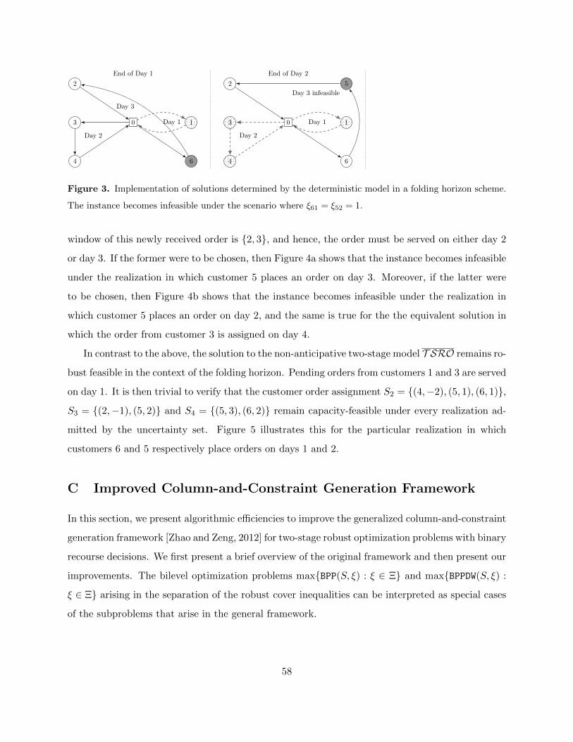
0 1

2

3

4 6

End of Day 1

Day 2

Day 1

Day 3

0 1

2

3

4

5

6

End of Day 2

Day 3 infeasible

Day 2

Day 1

Figure 3. Implementation of solutions determined by the deterministic model in a folding horizon scheme.

The instance becomes infeasible under the scenario where ξ61 = ξ52 = 1.

window of this newly received order is {2, 3}, and hence, the order must be served on either day 2

or day 3. If the former were to be chosen, then Figure 4a shows that the instance becomes infeasible

under the realization in which customer 5 places an order on day 3. Moreover, if the latter were

to be chosen, then Figure 4b shows that the instance becomes infeasible under the realization in

which customer 5 places an order on day 2, and the same is true for the the equivalent solution in

which the order from customer 3 is assigned on day 4.

In contrast to the above, the solution to the non-anticipative two-stage model T SRO remains ro-

bust feasible in the context of the folding horizon. Pending orders from customers 1 and 3 are served

on day 1. It is then trivial to verify that the customer order assignment S2 = {(4,−2), (5, 1), (6, 1)},

S3 = {(2,−1), (5, 2)} and S4 = {(5, 3), (6, 2)} remain capacity-feasible under every realization ad-

mitted by the uncertainty set. Figure 5 illustrates this for the particular realization in which

customers 6 and 5 respectively place orders on days 1 and 2.

C Improved Column-and-Constraint Generation Framework

In this section, we present algorithmic efficiencies to improve the generalized column-and-constraint

generation framework [Zhao and Zeng, 2012] for two-stage robust optimization problems with binary

recourse decisions. We first present a brief overview of the original framework and then present our

improvements. The bilevel optimization problems max{BPP(S, ξ) : ξ ∈ Ξ} and max{BPPDW(S, ξ) :

ξ ∈ Ξ} arising in the separation of the robust cover inequalities can be interpreted as special cases

of the subproblems that arise in the general framework.

58

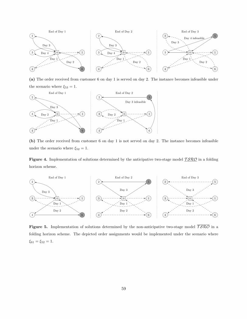
0 1

2

3

4 6

End of Day 1

Day 3

Day 2Day 1

Day 4 0 1

2

3

4 6

End of Day 2

Day 3

Day 2Day 1

Day 4 0 1

2

3

4

5

6

End of Day 3

Day 4 infeasible

Day 2

Day 3

Day 1

(a) The order received from customer 6 on day 1 is served on day 2. The instance becomes infeasible under

the scenario where ξ53 = 1.

0 1

2

3

4 6

End of Day 1

Day 1

Day 2

Day 3

0 1

2

3

4

5

6

End of Day 2

Day 3 infeasible

Day 1

Day 2

(b) The order received from customer 6 on day 1 is not served on day 2. The instance becomes infeasible

under the scenario where ξ52 = 1.

Figure 4. Implementation of solutions determined by the anticipative two-stage model T SRO in a folding

horizon scheme.

0 1

2

3

4 6

End of Day 1

Day 3

Day 1

Day 2

0 1

2

3

4

5

6

End of Day 2

Day 1

Day 2

Day 3

0 1

2

3

4

5

6

End of Day 3

Day 1

Day 2

Day 3

Figure 5. Implementation of solutions determined by the non-anticipative two-stage model T SRO in a

folding horizon scheme. The depicted order assignments would be implemented under the scenario where

ξ61 = ξ52 = 1.

59

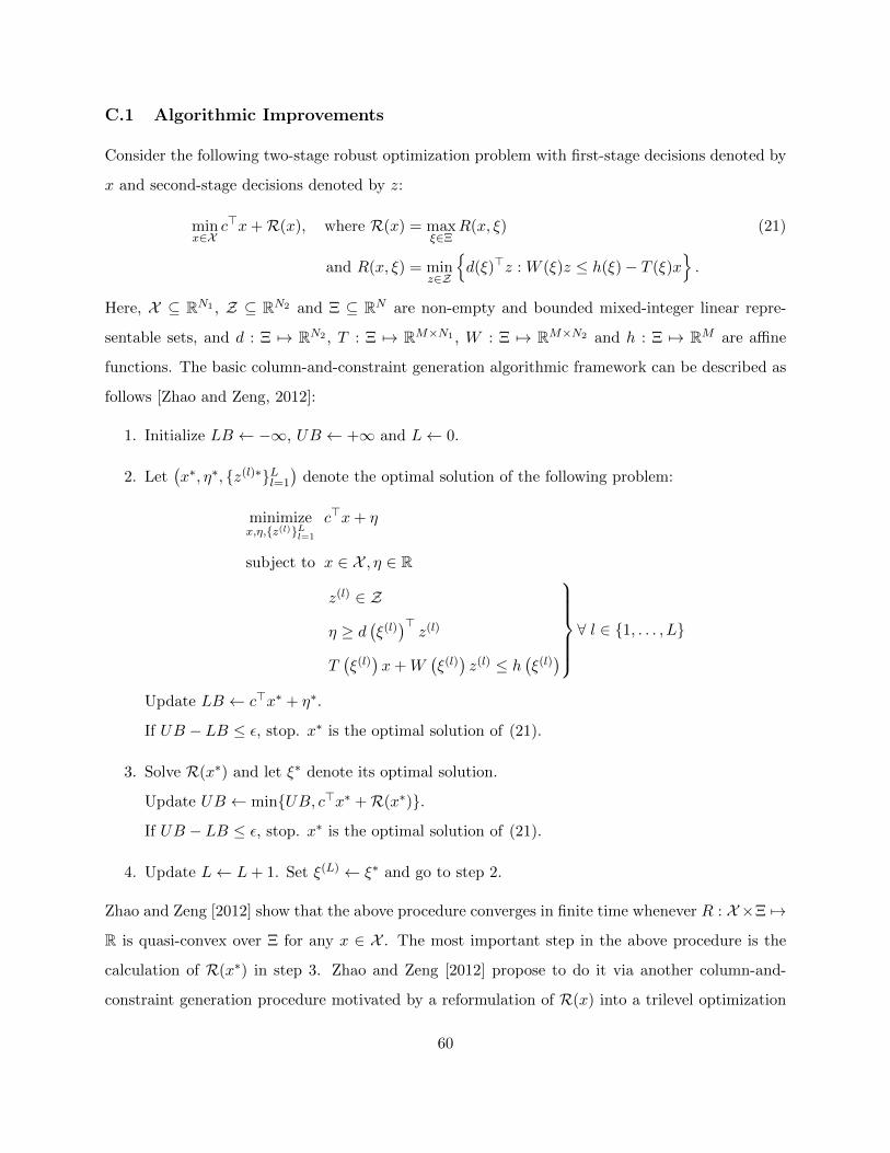
C.1 Algorithmic Improvements

Consider the following two-stage robust optimization problem with first-stage decisions denoted by

x and second-stage decisions denoted by z:

minx∈X

c>x+R(x), where R(x) = maxξ∈Ξ

R(x, ξ) (21)

and R(x, ξ) = minz∈Z

{d(ξ)>z : W (ξ)z ≤ h(ξ)− T (ξ)x

}.

Here, X ⊆ RN1 , Z ⊆ RN2 and Ξ ⊆ RN are non-empty and bounded mixed-integer linear repre-

sentable sets, and d : Ξ 7→ RN2 , T : Ξ 7→ RM×N1 , W : Ξ 7→ RM×N2 and h : Ξ 7→ RM are affine

functions. The basic column-and-constraint generation algorithmic framework can be described as

follows [Zhao and Zeng, 2012]:

1. Initialize LB ← −∞, UB ← +∞ and L← 0.

2. Let(x∗, η∗, {z(l)∗}Ll=1

)denote the optimal solution of the following problem:

minimizex,η,{z(l)}Ll=1

c>x+ η

subject to x ∈ X , η ∈ R

z(l) ∈ Z

η ≥ d(ξ(l))>z(l)

T(ξ(l))x+W

(ξ(l))z(l) ≤ h

(ξ(l))

∀ l ∈ {1, . . . , L}Update LB ← c>x∗ + η∗.

If UB − LB ≤ ε, stop. x∗ is the optimal solution of (21).

3. Solve R(x∗) and let ξ∗ denote its optimal solution.

Update UB ← min{UB, c>x∗ +R(x∗)}.

If UB − LB ≤ ε, stop. x∗ is the optimal solution of (21).

4. Update L← L+ 1. Set ξ(L) ← ξ∗ and go to step 2.

Zhao and Zeng [2012] show that the above procedure converges in finite time whenever R : X ×Ξ 7→

R is quasi-convex over Ξ for any x ∈ X . The most important step in the above procedure is the

calculation of R(x∗) in step 3. Zhao and Zeng [2012] propose to do it via another column-and-

constraint generation procedure motivated by a reformulation of R(x) into a trilevel optimization

60

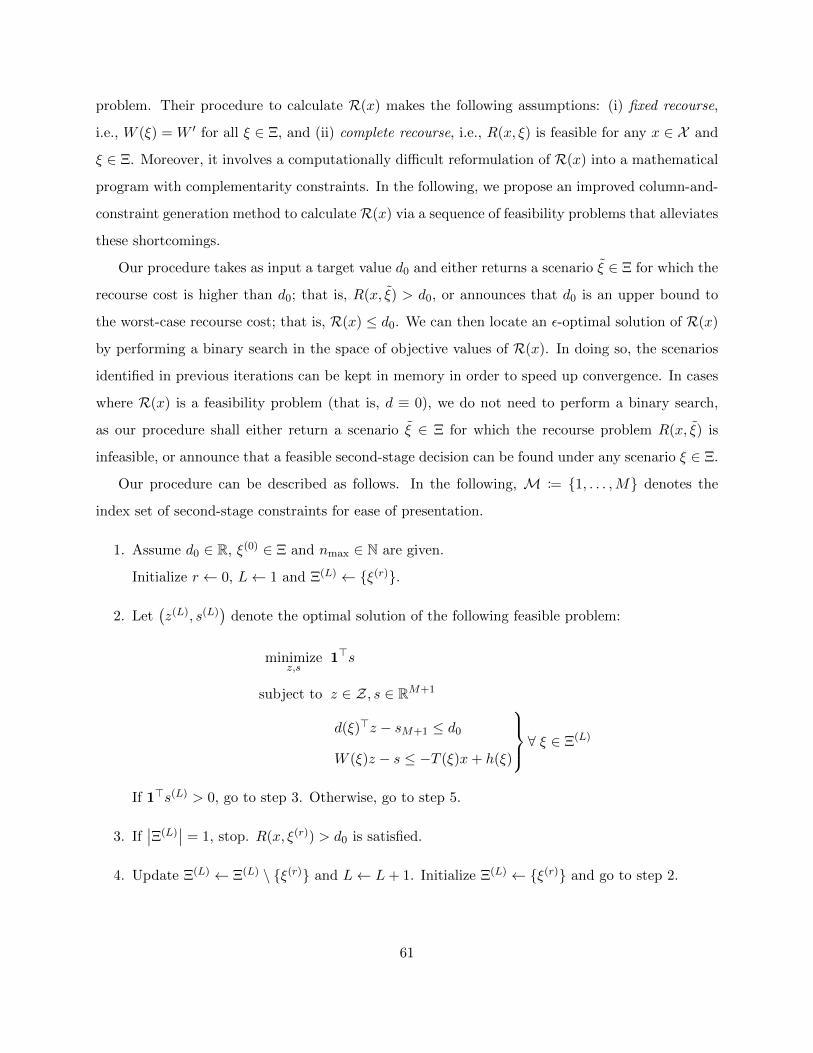
problem. Their procedure to calculate R(x) makes the following assumptions: (i) fixed recourse,

i.e., W (ξ) = W ′ for all ξ ∈ Ξ, and (ii) complete recourse, i.e., R(x, ξ) is feasible for any x ∈ X and

ξ ∈ Ξ. Moreover, it involves a computationally difficult reformulation of R(x) into a mathematical

program with complementarity constraints. In the following, we propose an improved column-and-

constraint generation method to calculate R(x) via a sequence of feasibility problems that alleviates

these shortcomings.

Our procedure takes as input a target value d0 and either returns a scenario ξ ∈ Ξ for which the

recourse cost is higher than d0; that is, R(x, ξ) > d0, or announces that d0 is an upper bound to

the worst-case recourse cost; that is, R(x) ≤ d0. We can then locate an ε-optimal solution of R(x)

by performing a binary search in the space of objective values of R(x). In doing so, the scenarios

identified in previous iterations can be kept in memory in order to speed up convergence. In cases

where R(x) is a feasibility problem (that is, d ≡ 0), we do not need to perform a binary search,

as our procedure shall either return a scenario ξ ∈ Ξ for which the recourse problem R(x, ξ) is

infeasible, or announce that a feasible second-stage decision can be found under any scenario ξ ∈ Ξ.

Our procedure can be described as follows. In the following, M := {1, . . . ,M} denotes the

index set of second-stage constraints for ease of presentation.

1. Assume d0 ∈ R, ξ(0) ∈ Ξ and nmax ∈ N are given.

Initialize r ← 0, L← 1 and Ξ(L) ← {ξ(r)}.

2. Let(z(L), s(L)

)denote the optimal solution of the following feasible problem:

minimizez,s

1>s

subject to z ∈ Z, s ∈ RM+1

d(ξ)>z − sM+1 ≤ d0

W (ξ)z − s ≤ −T (ξ)x+ h(ξ)

∀ ξ ∈ Ξ(L)

If 1>s(L) > 0, go to step 3. Otherwise, go to step 5.

3. If∣∣Ξ(L)

∣∣ = 1, stop. R(x, ξ(r)) > d0 is satisfied.

4. Update Ξ(L) ← Ξ(L) \ {ξ(r)} and L← L+ 1. Initialize Ξ(L) ← {ξ(r)} and go to step 2.

61

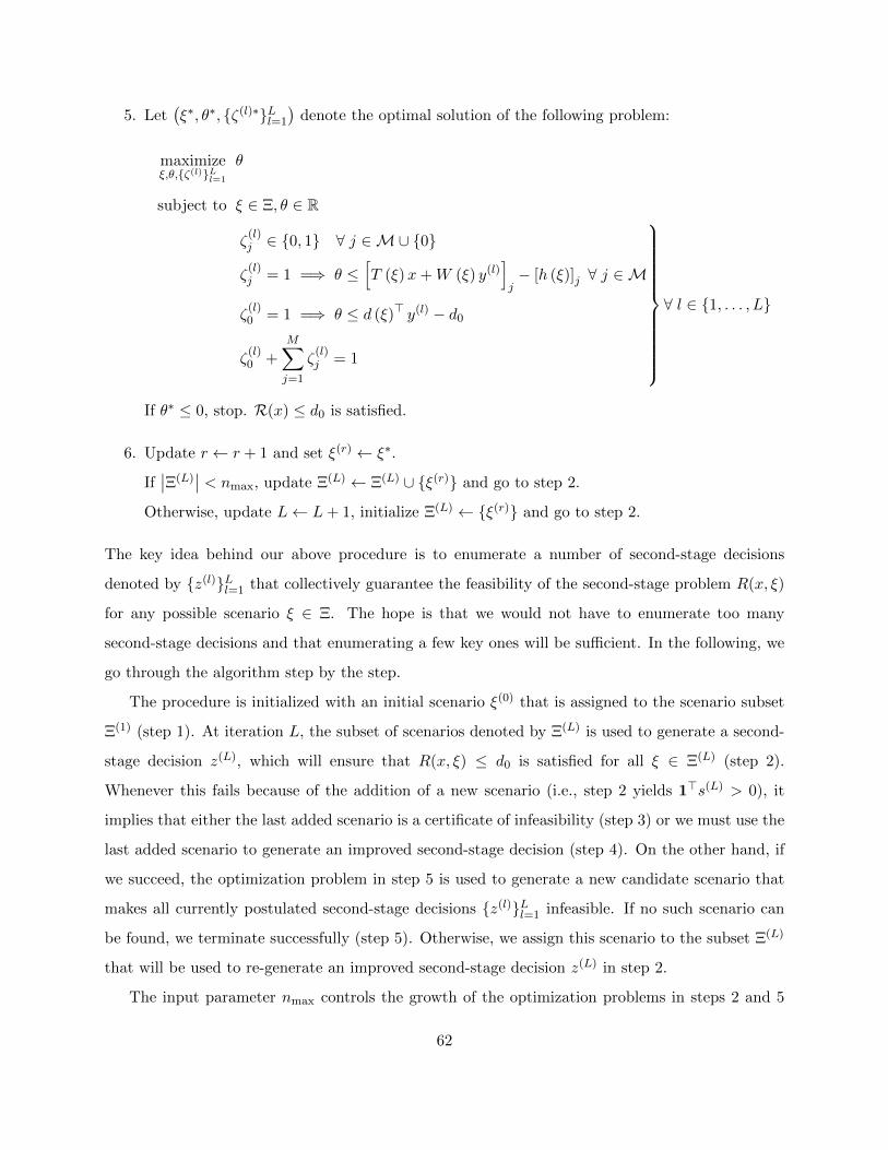
5. Let(ξ∗, θ∗, {ζ(l)∗}Ll=1

)denote the optimal solution of the following problem:

maximizeξ,θ,{ζ(l)}Ll=1

θ

subject to ξ ∈ Ξ, θ ∈ R

ζ(l)j ∈ {0, 1} ∀ j ∈M∪ {0}

ζ(l)j = 1 =⇒ θ ≤

[T (ξ)x+W (ξ) y(l)

]j− [h (ξ)]j ∀ j ∈M

ζ(l)0 = 1 =⇒ θ ≤ d (ξ)> y(l) − d0

ζ(l)0 +

M∑j=1

ζ(l)j = 1

∀ l ∈ {1, . . . , L}

If θ∗ ≤ 0, stop. R(x) ≤ d0 is satisfied.

6. Update r ← r + 1 and set ξ(r) ← ξ∗.

If∣∣Ξ(L)

∣∣ < nmax, update Ξ(L) ← Ξ(L) ∪ {ξ(r)} and go to step 2.

Otherwise, update L← L+ 1, initialize Ξ(L) ← {ξ(r)} and go to step 2.

The key idea behind our above procedure is to enumerate a number of second-stage decisions

denoted by {z(l)}Ll=1 that collectively guarantee the feasibility of the second-stage problem R(x, ξ)

for any possible scenario ξ ∈ Ξ. The hope is that we would not have to enumerate too many

second-stage decisions and that enumerating a few key ones will be sufficient. In the following, we

go through the algorithm step by the step.

The procedure is initialized with an initial scenario ξ(0) that is assigned to the scenario subset

Ξ(1) (step 1). At iteration L, the subset of scenarios denoted by Ξ(L) is used to generate a second-

stage decision z(L), which will ensure that R(x, ξ) ≤ d0 is satisfied for all ξ ∈ Ξ(L) (step 2).

Whenever this fails because of the addition of a new scenario (i.e., step 2 yields 1>s(L) > 0), it

implies that either the last added scenario is a certificate of infeasibility (step 3) or we must use the

last added scenario to generate an improved second-stage decision (step 4). On the other hand, if

we succeed, the optimization problem in step 5 is used to generate a new candidate scenario that

makes all currently postulated second-stage decisions {z(l)}Ll=1 infeasible. If no such scenario can

be found, we terminate successfully (step 5). Otherwise, we assign this scenario to the subset Ξ(L)

that will be used to re-generate an improved second-stage decision z(L) in step 2.

The input parameter nmax controls the growth of the optimization problems in steps 2 and 5

62

by controlling the maximum cardinality of Ξ(L). The choice nmax = 1 would create new variables

and constraints in the optimization problem of step 5 every time it is performed, but would restrict

the size of the problem in step 2 to involve constraints for just one scenario. On the other hand,

nmax = +∞ would create new variables and constraints in the optimization problem of step 5 only

when necessary, but would involve constraints for each scenario in Ξ(L). Higher values of nmax are

preferable since the complexity of the optimization problem in step 2 can typically be managed

using cutting plane techniques, if necessary.

We remark that the procedure converges in finite time whenever Z or Ξ are finite sets. We

reason as follows. By construction, the separation problem in step 5 can only generate a scenario

ξ(r) that makes all currently generated second-stage decisions {z(l)}Ll=1 infeasible. This scenario is

then assigned to one of the scenario subsets {Ξ(l)}Ll=1 in a way that ensures it is never identified

again in step 5 in subsequent iterations (unless the procedure terminates in step 3). Consequently,

no scenario is generated more than once in step 5. Moreover, by the same reasoning, no second-stage

decision is generated more than once in step 2 (unless the procedure terminates in step 3).

C.2 Solving max {BPP(S, ξ) : ξ ∈ Ξ} and max {BPPDW(S, ξ) : ξ ∈ Ξ}

Observe that these problems are special cases of R(x) in which the recourse problem R(x, ξ) is a

Bin Packing Problem, and a Bin Packing Problem with Day Windows respectively. Therefore, we

can utilize any integer programming formulation of BPP(S, ξ) or BPPDW(S, ξ) to replace R(x, ξ) in the

previously described procedure to obtain their maxima. However, we improve numerical tractability

in two ways: (i) we utilize an associated feasibility-based integer programming formulation of these

problems, and (ii) we do not attempt to obtain the true maxima of these problems.

More specifically, we consider the following integer programing formulation associated with

BPP(S, ξ), which either determines a capacity-feasible assignment of items in S to at most m bins,

or results in infeasibility implying that the optimal value of the bin packing problem exceeds m.

63

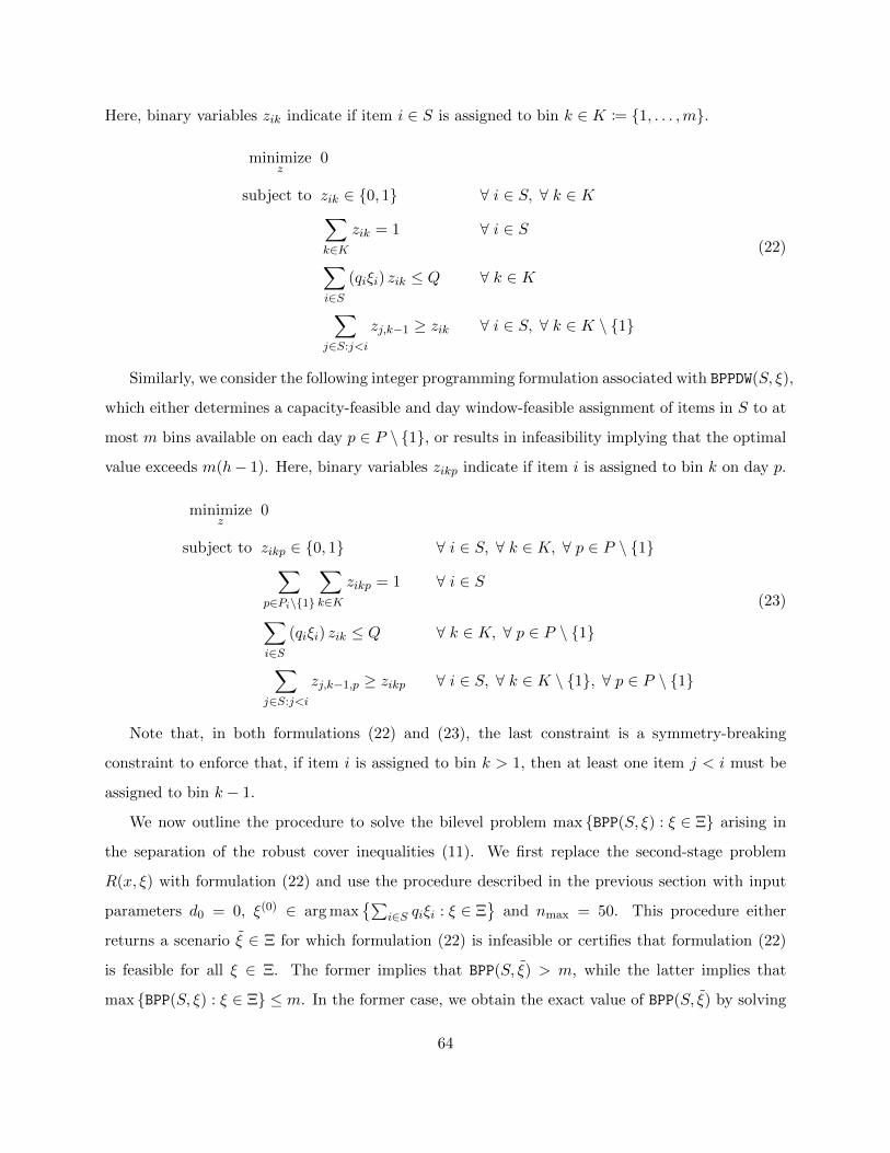
Here, binary variables zik indicate if item i ∈ S is assigned to bin k ∈ K := {1, . . . ,m}.

minimizez

0

subject to zik ∈ {0, 1} ∀ i ∈ S, ∀ k ∈ K∑k∈K

zik = 1 ∀ i ∈ S

∑i∈S

(qiξi) zik ≤ Q ∀ k ∈ K

∑j∈S:j<i

zj,k−1 ≥ zik ∀ i ∈ S, ∀ k ∈ K \ {1}

(22)

Similarly, we consider the following integer programming formulation associated with BPPDW(S, ξ),

which either determines a capacity-feasible and day window-feasible assignment of items in S to at

most m bins available on each day p ∈ P \ {1}, or results in infeasibility implying that the optimal

value exceeds m(h− 1). Here, binary variables zikp indicate if item i is assigned to bin k on day p.

minimizez

0

subject to zikp ∈ {0, 1} ∀ i ∈ S, ∀ k ∈ K, ∀ p ∈ P \ {1}∑p∈Pi\{1}

∑k∈K

zikp = 1 ∀ i ∈ S

∑i∈S

(qiξi) zik ≤ Q ∀ k ∈ K, ∀ p ∈ P \ {1}

∑j∈S:j<i

zj,k−1,p ≥ zikp ∀ i ∈ S, ∀ k ∈ K \ {1}, ∀ p ∈ P \ {1}

(23)

Note that, in both formulations (22) and (23), the last constraint is a symmetry-breaking

constraint to enforce that, if item i is assigned to bin k > 1, then at least one item j < i must be

assigned to bin k − 1.

We now outline the procedure to solve the bilevel problem max {BPP(S, ξ) : ξ ∈ Ξ} arising in

the separation of the robust cover inequalities (11). We first replace the second-stage problem

R(x, ξ) with formulation (22) and use the procedure described in the previous section with input

parameters d0 = 0, ξ(0) ∈ arg max{∑

i∈S qiξi : ξ ∈ Ξ}

and nmax = 50. This procedure either

returns a scenario ξ ∈ Ξ for which formulation (22) is infeasible or certifies that formulation (22)

is feasible for all ξ ∈ Ξ. The former implies that BPP(S, ξ) > m, while the latter implies that

max {BPP(S, ξ) : ξ ∈ Ξ} ≤ m. In the former case, we obtain the exact value of BPP(S, ξ) by solving

64

a deterministic bin packing problem using the exact algorithm MTP described in Martello and Toth

[1990] and use the resulting value when adding the corresponding robust cover inequality (11).

We remark that, in both outcomes, the exactness of the separation algorithm for the robust cover

inequalities (11) is guaranteed.

The procedure to solve max {BPPDW(S, ξ) : ξ ∈ Ξ} arising in the separation of inequalities (18)

is exactly the same, except that we replace the second-stage problem R(x, ξ) with formulation (23).

Moreover, in the case when we have identified a scenario ξ ∈ Ξ for which BPPDW(S, ξ) > m(h− 1),

we do not compute the exact value of BPPDW(S, ξ) but rather use the lower bound of m(h− 1) + 1

when adding the corresponding inequality (18), since our computational experience suggested that

the optimal value of BPPDW(S, ξ) almost never exceeds this lower bound. We remark that this does

not invalidate the correctness of the lower bounds provided by formulation T SROIP .

65