Embed Size (px)
Citation preview
Robust Model Selection and Outlier Detectionin Linear Regression
by
Lauren McCann
S.B. Mathematics, Massachusetts Institute of Technology, 2001
Submitted to the Sloan School of Managementin partial fulfillment- of the requirements for the degree of
Doctor of Philosophy in Operations Research
at the
MASSACHUSETTS INSTITUTE OF TECHNOLOGY
June 2006
( Massachusetts Institute of Technology 2006. All rights reserved.
Author ................................. ...................Sloan School of Management
May 18, 2006
Certified by.......................... ........ Roy ... ........... elschRoy E. Welsch
Professor of Statistics, Management Science,and Engineering Systems, MIT
Thesis Supervisor
Accepted by ................................James B. Orlin
Edward Pennell Brooks Professor of Operations Research, MIT
MASSACHUSETMTS INSTtITUTEOF TECHNOLOGY
JUL 2 4 2006
LIBRARIES
MCHIovE
Codirector, Operations Research Center, MIT

Robust Model Selection and Outlier Detection
in Linear Regression
by
Lauren McCann
Submitted to the Sloan School of Managementon May 18, 2006, in partial fulfillment of the
requirements for the degree ofDoctor of Philosophy in Operations Research
AbstractIn this thesis, we study the problems of robust model selection and outlier detectionin linear regression. The results of data analysis based on linear regressions are highlysensitive to model choice and the existence of outliers in the data. This thesis aims tohelp researchers to choose the correct model when their data could be contaminatedwith outliers, to detect possible outliers in their data, and to study the impact thatsuch outliers have on their analysis.
First, we discuss the problem of robust model selection. Many methods for per-forming model selection were designed with the standard error model ( - N(0, a2 ))and least squares estimation in mind. These methods often perform poorly on realworld data, which can include outliers. Robust model selection methods aim to pro-tect us from outliers and capture the model that represents the bulk of the data.
We review the currently available model selection algorithms (both non-robustand robust) and present five new algorithms. Our algorithms aim to improve uponthe currently available algorithms, both in terms of accuracy and computational fea-sibility. We demonstrate the improved accuracy of our algorithms via a simulationstudy and a study on a real world data set.
Finally, we discuss the problem of outlier detection. In addition to model selec-tion, outliers can adversely influence many other outcomes of regression-based dataanalysis. We describe a new outlier diagnostic tool, which we call diagnostic datatraces. This tool can be used to detect outliers and study their influence on a vari-ety of regression statistics. We demonstrate our tool on several data sets, which areconsidered benchmarks in the field of outlier detection.
Thesis Supervisor: Roy E. WelschTitle: Professor of Statistics, Management Science,and Engineering Systems, MIT
3

4

Acknowledgments
I would like to especially thank the following people for their help, support, and guid-
ance in graduate school and in completing this thesis:
My advisor - Roy Welsch
My committee - Arnold Barnett and Alexander Samarov
My husband - Gabriel Weinberg
My parents - Maureen and Gerald McCann
My sister and brother-in-law - Tara McCann and Brian Spadora
My kitties - Isaac and Thomas
My ORC friends
5

6

Contents
1 Introduction
1.1 Problem Description: Robust Model Selection
1.1.1 Why Model Selection?.
1.1.2 Why Robust? .
1.2 Problem Description: Outlier Detection ....
1.3 Overview of the Thesis .............
1.3.1 Contributions.
1.3.2 Outline .................
2 Literature Review
2.1 Model Selection Methods for the Standard Regression
2.1.1 The Need for Robustness ............
2.2 Robustness Ideas in Regression ............
2.3 Robust Model Selection.
Model
3 Sampling-only Algorithms for Robust Model Selection
3.1 Elemental Set Sampling and Robustness ................
3.2 Draws Algorithm.
3.3 LARS Draws ...............................
3.3.1 Background: Least Angle Regression and the LARS Algorithm
3.3.2 The LARS Draws Algorithm ...................
3.3.3 Parameter Choices ........................
7
19
19
21
22
23
25
25
26
29
29
32
33
35
37
37
38
39
39
41
43
..........................
.............
.............
.............
.............
.............

4 Model Selection using the Mean-Shift Outlier Model and Penalty
Methods
4.1 Motivations.
4.2 Constraining the System.
4.2.1 History of Penalization ...............
4.3 Constraints and Lagrangian Relaxation ..........
4.4 Bayesian Interpretation .
5 A Detailed Look At Using Different Penalty Functions
5.1 Simple Ridge Penalty and the Pen Algorithm ........
5.1.1 Bayesian Interpretation of Ridge Regression .....
5.1.2 Selection .........................
5.1.3 The Pen Algorithm ...................
5.2 Non-equivalence in Priors ...................
5.2.1 The Nonzero Mean Prior (NZMP) Pen Algorithm . .
5.3 LASSO and LARS .......................
5.3.1 Bayesian Interpretation of the Lasso Penalty .....
5.3.2 Benefits of LASSO Over Ridge ............
5.3.3 Least Angle Regression: A Close Relative of LASSO
5.3.4 The Simple dLASSO/dLARS Pen Algorithm .....
5.3.5 The Sample dLASSO/dLARS Pen Algorithm .
5.3.6 dLARS Draws ......................
6 Evaluating the Algorithms' Performances
6.1 Simulations.
6.1.1 Results and Conclusions .......
6.1.2 An Alternative Correctness Measure
6.2 Mortality Data ................
6.2.1 Selected Models ............
6.2.2 Which model is best? .........
6.2.3 Simulations vs. Real Data ......
85
............. . .86. . . . . . . . . . . . . . 87
.. . . . . . . . . . . . . 99
... . . . .. .. .. .. 102
... . . . .. . . .. . . 103
... .. . . . . .. . .. 104
... . . . . . .. .. .. 108
8
49
49
50
53
56
57
59
... . 59
... . 61
... . 63
... . 64
... . 66
... . 67
... . 72
... . 73
... . 75
... . 76.... 77
... . 80
... . 82
7 Diagnostic Traces and Forward Search
7.1 Outlier Detection.
7.2 Forward Search.
7.2.1 The Forward Search Algorithm .........
7.3 Diagnostic Data Traces Using Ridge Penalty Methods .
7.3.1 Initial Subset.
7.3.2 Adding Back Data Points ............
7.3.3 Plotting ......................
7.3.4 Where to Look ..................
7.4 Example: Hawkins Data .................
7.4.1 Hawkins Data ...................
7.5 Comparing Forward Search to Diagnostic Data Traces
Penalty.
7.6 Example: The Rousseeuw Data .............
7.6.1 The Belgian Phone Data .............
7.6.2 The Hertzsprung-Russell Star Data .......
7.7 Diagnostic Data Traces Using LARS ..........
7.7.1 LARS vs. LASSO .................
7.7.2
7.7.3
A Data Sets
The Diagnostic Data Traces with LARS/LASSO
Plotting.
with a Ridge
Algorithm
B Tables
C Comparison of Forward Search plots and Diagnostic Data Traces
using the Ridge Penalty 177
D Complete Set of Diagnostic Data Traces using the Ridge Penalty for
the Belgian Phone Data 185
9
109
109
112
112
117
119
120
127
128
130
130
144
147
147
151
158
160
161
161
167
175

10
List of Figures
1-1 A Demonstration of Zero Breakdown of Ordinary Least Squares: As
we move the point (3, 0) from its original position to (25, 0) and (50, 0)
we see the regression line flatten. We can make this line arbitrarily
close to y = 0 if we continue moving the point along the x axis. ... . 23
5-1 This is a two-dimensional example estimation picture for the lasso (di-
amond) and ridge regression (circle). The diamond is the lasso con-
straint, Il I+ 1/321 < t. The circle is the ridge constraint, P2 + /3 < t.
The ellipses are the contours of the least squares error function. The or-
dinary least squares solution is the unrestricted minimum, represented
by the dot in the center of the contours. The sum of squares increase
as we move away from the center. Notice how, when the error is mini-
mized within the lasso constraint, the minimum occurs at a vertex. In
contrast, when ridge constraint it considered, we can find a lower error
that is not at one of the axes. ...................... 74
5-2 This figure shows the differences in shape between the normal (prior
for ridge) and double exponential (prior for LASSO) distributions. .. 75
7-1 Hawkins Data: Forward Search plots of m vs. P(m) and m vs. t(P(m))
as computed by the forward library for S-Plus .............. 115
7-2 Hawkins Data: Forward Search plot of m vs. (m))/sful as computed
by the forward library for S-Plus. ..................... . 116
7-3 Hawkins Data: Forward Search plot of m vs. ((m)) 2/s2fl as computed
by the forward library for S-Plus. ..................... . 116
11

7-4 Hawkins Data: Forward Search plot of m vs. sI(m) as computed by the
forward library for S-Plus ......................... 117
7-5 Hawkins Data: Forward Search plots of m vs. Maximum Studentized
Residuals and m vs. Minimum Deletion Residuals as computed by the
forward library for S-Plus. ......................... 118
7-6 Hawkins Data: Forward Search plots of m vs. Leverage (diagonals
of the hat matrix for the current subset) as computed by the forward
library for S-Plus .............................. 118
7-7 Hawkins Data: Diagnostic Data Trace using the Ridge Penalty plot of
of subset size m vs. Scaled Residuals . ................. 131
7-8 Hawkins Data: Diagnostic Data Trace using the Ridge Penalty plot of
subset size m vs. Squared Scaled Residuals . .............. 132
7-9 Hawkins Data: Diagnostic Data Trace using the Ridge Penalty plot of
subset size m vs. Scaled Residuals for just the "good" points in the
initial subset Nq . . . . . . . . . . . . . . . . . ........... 134
7-10 Hawkins Data: Diagnostic Data Trace using the Ridge Penalty plot of
subset size m vs. Prediction Residuals on the points in Nq ...... 136
7-11 Hawkins Data: Diagnostic Data Trace using the Ridge Penalty plot of
subset size m vs. Prediction Score . ................... 136
7-12 Hawkins Data: Diagnostic Data Trace using the Ridge Penalty plot of
subset size log1 0 A vs. Prediction Score (A) . .............. 137
7-13 Hawkins Data: Diagnostic Data Trace using the Ridge Penalty plot of
subset size subset size m vs. s2 ................... .. 138
7-14 Hawkins Data: Diagnostic Data Trace using the Ridge Penalty plot of
subset size subset size m vs. the estimates of the coefficients ..... 140
7-15 Hawkins Data: Diagnostic Data Trace using the Ridge Penalty plot of
subset size subset size m vs. the T-statistics . ............. 140
7-16 Hawkins Data: Diagnostic Data Traces using the Ridge Penalty plots
of subset size m vs. the Maximum Studentized Residual and subset
size subset size m vs. the Minimum Deletion Residual ......... 142
12

7-17 Hawkins Data: Diagnostic Data Traces using the Ridge Penalty plot
of subset size m vs. leverage on each non-outlying point as measured
by the diagonals of the Hat matrix ................... 143
7-18 Two Plots Depicting the Non-linear Relationship Between Subset Size
and A: The first plot shows us that searching over a linear grid of
As would be very inefficient. Also depending on the grid size, we will
either miss smaller subset sizes on the low end or move way too slowly
through the high end. The second plot shows us that subset size is
more likely related to log(A). This second plot is not linear though.
Note however, that this plot has three fairly linear regions separated
by flat regions that correspond exactly to when outlier groups enter
the "good" subset ............................. 145
7-19 Belgian Phone Data ........................... 148
7-20 Belgian Phone Data: Diagnostic Trace from Ridge Penalty ...... 149
7-21 Belgian Phone Data: Diagnostic Trace from Ridge Penalty ...... 150
7-22 Belgian Phone Data: Diagnostic Trace from Ridge Penalty ...... 150
7-23 Hertzsprung-Russell Data from the Star Cluster CYG OB1 ...... 152
7-24 H-R Star Data: Diagnostic Data Traces using the Ridge Penalty plot
of subset size m vs. Scaled Squared Residuals ............. 153
7-25 H-R Star Data: Diagnostic Data Traces using the Ridge Penalty zoomed
in plot of subset size m vs. Scaled Squared Residuals - In this plot,
we have zoomed in at the end of the plot to get a better view of what
happens once the outliers have been added to the subset used to fit the
coefficients. Some of the outliers are masked and some of the original
good points are swamped. ............ ............ 154
7-26 H-R Star Data: Diagnostic Data Traces using the Ridge Penalty plots
of subset size m vs. the Hat matrix diagonals for the points in the
non-outlier subset, which are a measure of leverage .......... 156
13
7-27 H-R Star Data: Diagnostic Data Traces using the Ridge Penalty plots
of subset size m vs. the Maximum Studentized Residual and subset
size subset size m vs. the Minimum Deletion Residual ......... 157
7-28 H-R Star Data: Diagnostic Data Traces using LARS plots of subset
size m vs. scaled residuals ........................ 163
7-29 H-R Star Data: Diagnostic Data Traces using LARS plots of subset
size m vs. squared scaled residuals ................... 163
7-30 H-R Star Data: Diagnostic Data Traces using LARS plots of subset
size m vs. scaled residuals from the initial set, Nq .......... . 164
7-31 H-R Star Data: Diagnostic Data Traces using LARS plots of subset size
m vs. the estimated beta coefficients and subset size m vs. t-statistics 164
7-32 H-R Star Data: Diagnostic Data Traces using LARS plots of subset
size m vs. the Maximum Studentized Residual and subset size subset
size m vs. the Minimum Deletion Residual ............... 165
7-33 H-R Star Data: Diagnostic Data Traces using LARS plots of subset
size m vs. s2 ................................ 165
7-34 H-R Star Data: Diagnostic Data Traces using LARS plots of subset
size m vs. ................................. 166
C-1 Comparison between Forward Search (top) and our Diagnostic Data
Traces using the Ridge Penalty (bottom) by Example (Hawkins Data):
subset size vs. Fitted Coefficients - Note: the Forward Search plot is
of scaled coefficients. Our plot looks most similar to the plot in Figure
3.4 in [5], which we have not gotten copyright permission to reproduce. 178
C-2 Comparison between Forward Search (top) and our Diagnostic Data
Traces using the Ridge Penalty (bottom) by Example (Hawkins Data):
subset size vs. Scaled Residuals ................... .. 179
C-3 Comparison between Forward Search (top) and our Diagnostic Data
Traces using the Ridge Penalty (bottom) by Example (Hawkins Data):
subset size vs. Scaled Squared Residuals ................ 180
14
C-4 Comparison between Forward Search (top) and our Diagnostic Data
Traces using the Ridge Penalty (bottom) by Example (Hawkins Data):
subset size vs. s2 and subset size vs. R2 ................
C-5 Comparison between Forward Search (top) and our Diagnostic Data
Traces using the Ridge Penalty (bottom) by Example (Hawkins Data):
subset size vs. maximum studentized residuals and subset size vs.
minimum deletion residuals .......................
C-6 Comparison between Forward Search (top) and our Diagnostic Data
Traces using the Ridge Penalty (bottom) by Example (Hawkins Data):
subset size vs. Leverage .........................
Belgian Phone Data:
Belgian Phone Data:
Belgian Phone Data:
Belgian Phone Data:
Belgian Phone Data:
Belgian Phone Data:
Belgian Phone Data:
Belgian Phone Data:
Diagnostic Trace from Ridge Penalty
Diagnostic Trace from Ridge Penalty
Diagnostic Trace from Ridge Penalty
Diagnostic Trace from Ridge Penalty
Diagnostic Trace from Ridge Penalty
Diagnostic Trace from Ridge Penalty
Diagnostic Trace from Ridge Penalty
Diagnostic Trace from Ridge Penalty
... . . . 186
... . . . 186
... . . . 187
... . . . 188
... . . . 188
... . . . 189
... . . . 189
... . . . 190
15
181
182
183
D-1
D-2
D-3
D-4
D-5
D-6
D-7
D-8

16

List of Tables
4.1 Data Formulation ............................. 50
5.1 Data Formulation ............................. 60
6.1 Simulation Results: Algorithm Performance .............. 88
6.2 Simulation Results: Algorithm Performance Averaged Over Error Types 90
6.3 Simulation Results: Draws-type Algorithm Comparison - M = 500
and n = 8 ................................. 94
6.4 Simulation Results: Draws-type Algorithm Comparison - M = 2000
and n = 8 ............. . ................... 95
6.5 Simulation Results: Draws-type Algorithm Comparison (M = 500) -
Finding Overall Results by Summing Across Error Models ...... 96
6.6 Simulation Results: Draws-type Algorithm Comparison (M = 2000) -
Finding Overall Results by Summing Across Error Models ...... 96
6.7 Simulation Results: These are the results of a simulation comparing
our dLARS Simple algorithm to the algorithms from Khan et. al. [34]
when considering their alternative measure of correctness ........ 101
6.8 Models Selected from Various Algorithms ................ 103
6.9 Comparing Models by Robust Measures of Goodness of Fit ...... 105
6.10 Best Subsets Scores on Cleaned Data .................. 106
6.11 Prediction Scores of Models based on Cross-Validation ........ 107
A.1 Hawkins Data ............................... 168
A.2 Hawkins Data Continued. . . . . . . . . . . . . . ...... 169
17

A.3 Hawkins Data Continued ......................... 170
A.4 Hawkins Data Continued ......................... 171
A.5 Belgian Phone Data ........................... 172
A.6 Hertzsprung-Russell Star Data . . . . . . . . . . . . . . . . . . . 173
A.7 Hertzsprung-Russell Star Data Continued . . . . . . . . . . . ..... 174
B.1 Results of simulations to the test the dLARS orderings as in Khan et.
al. [34] ................................... 175
B.2 Comparison of the CPU Time Required to Perform the Main Calcula-
tions in Forward Search and Diagnostic Data Traces on the Hawkins
Data .................................... 176
18

Chapter 1
Introduction
Regression analysis is the most widely used technique for fitting models to data [5],
[20]. When a regression model is fit using ordinary least squares, we get a few statistics
to describe a large set of data. These statistics can be highly influenced by a small
set of data that is different from the bulk of the data. These points could be y-type
outliers (vertical outliers) that do not follow to the general model of the data or x-
type outliers (leverage points) that are systematically different from the rest of the
explanatory data. We can also have points that are both leverage points and vertical
outliers, which are sometimes referred to as bad leverage points. Collectively, we call
any points of these kinds outliers.
In this thesis, we are interested both in detecting these points and in the effects
of such outliers and leverage points on model selection procedures. Given that the
model selection tools for the standard regression model are not sufficient in this case,
we plan to present some new robust algorithms for model selection. We will also
present some diagnostic tools to help detect possible outliers and study their impact
on various regression statistics.
1.1 Problem Description: Robust Model Selection
Given observations y = (yl,..., y,,) E Rn and corresponding instances of explanatory
variables x E RP,..., Xn E R, we want to model the relationship between y and
19
a subset of x E RP,.. ., xn E RP. In particular, we consider linear functions of the
explanatory variable to model and predict values of the outcome,
i= f0 + i 1,... (1.1)
with regression coefficients 3o, 31,..., p-1. Additionally we assume that the obser-
vations are observations of the form
Y = E(Yi xi) + ei, i = 1,...,n, (1.2)
where l,..., E, are independent and identically distributed with a common mean
and variance a2 .
In the standard regression model, i - Normal (0, a2). In general, the errors can
come from any distribution. We could model the errors as a mixture of Gaussian
errors and some general distribution G: ei , (1 - A) Normal (0, a 2) + AG, where
0 < A < 1. The standard regression model is the special case when A = 0. Many
types of y-type outliers can be modeled as part of this more general error model. In
these cases, most of the data follows the standard model (i.e. A < .5), but a few
outliers could be modeled as coming from a different distribution, possibly one with
a larger variance or a non-zero mean. A third possibility is that A = 1 and our data
did not have Gaussian error at all.
In the model selection problem, there is uncertainty in which subset of explanatory
variables to use. This problem is of particular interest when the number p of variables
is large and the set is thought to include irrelevant and/or redundant variables. Given
we are fitting a model of the form (1.1), a model selection technique should determine
which subset of the p explanatory variables truly have nonzero coefficients and which
have coefficients of zero. That is, if we force this subset of variables to have nonzero
coefficients and the others to have zero coefficients, we can create an accurate linear
predictor of the type (1.1) using these variables. This is a fundamental problem in
data analysis and is not restricted to linear regression or the field of statistics.
20

1.1.1 Why Model Selection?
Efficient model selection algorithms are useful for several reasons. Model selection
allows us to understand which variables (these can include functions of variables)
are "important". We are often looking for a better understanding of the underlying
process that generated our data.
Another reason is model simplicity. Given we would like to explain the functional
relationship between the explanatory variables and the outcome variable, simplicity is
desired because simpler explanations are easier to understand and interpret. We can
also learn something about what information is necessary to make a good prediction.
Money and time can be saved by reducing the amount of data we collect to just what
is absolutely necessary.
Prediction performance can also be improved through model selection. When
models are fit by least squares regression, each additional coefficient we add to a
model adds to the variance of the final regression equation. (Note: we are referring to
the actual variance and not the estimated variance.) So the fewer the coefficients we
estimate the lower the variance. The smallest possible model is to fit no parameters.
Our regression equation is then y = 0. This is a constant and thus has the minimum
variance of zero. Likewise selecting too few variables will lead to a biased answer.
We rely on a model selection tool to choose just the right number of variables, small
enough to have a low variance, but large enough to still get good predictions. (See
[43] if you would like to see a proof.)
Given we are going to select a model from p possible explanatory variables, there
are 2p such models to consider initially. Kadane and Lazar [33] point out that another
reason we need good model selection methods is to just reduce the amount of time
that would be spent if we seriously considered all of these models. Many times we
don't need to narrow the choices down to just one model. Sometimes it is sufficient to
"deselect" the models that are obviously the worst ones, narrowing the possibilities
down to a manageable set. Time savings in the model selection process brought by
efficient algorithms will also lead to cost savings.
21

1.1.2 Why Robust?
The model selection problem is well-studied for the standard error model, however
this problem is more difficult if we consider a general error distribution and possible
leverage points. Most of the standard model selection techniques rely in some way on
least squares. It is well known that many estimation techniques, like ordinary least
squares, do not treat all observations as equally important. This allows our choice of
model to be highly influenced by just a few points.
One measure of the robustness of an estimator is its breakdown point. The break-
down point is defined as the proportion of points used to fit an estimator that can
be changed, while not changing the estimator by an arbitrary amount. If a fraction
of the data than of equal to the breakdown point is contaminated, the estimated
statistic will not change too much. It is possible to change the estimated statistic to
another arbitrary value by appropriately changing a fraction of data larger than the
breakdown point.
The best breakdown we can get is 50% and the worst is 0%. Ordinary least squares
has a breakdown point of zero. If we appropriately change just one point, we can make
the regression coefficients change to make sure that we fit this point almost exactly
at the expense of fitting the rest of the points well. We demonstrate this breakdown
problem with OLS via a pictorial example in Figure 1-1. Our ordinary least squares
regression ends up working hard to fit this one point and ends up practically ignoring
the others.
Belsley, Kuh, and Welsch [8] formally define an influential observation as,
"one which, either individually or together with several other observations,
has a demonstrably larger impact on the calculated values of various es-
timates ... than is the case for most other observations."
Not all outliers are influential and not all influential points will hurt our modelling,
but we still need robust methods to prevent possible influential outliers and bad
leverage points from leading us to the wrong choice of model.
Statisticians who neglect to consider robust methods are ignoring the fact that
22
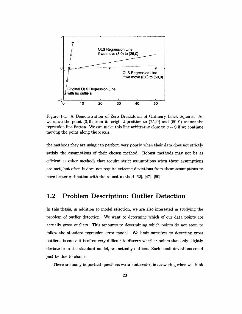
5
0
0 10 20 30 40 50
Figure 1-1: A Demonstration of Zero Breakdown of Ordinary Least Squares: Aswe move the point (3,0) from its original position to (25,0) and (50,0) we see theregression line flatten. We can make this line arbitrarily close to y = 0 if we continuemoving the point along the x axis.
the methods they are using can perform very poorly when their data does not strictly
satisfy the assumptions of their chosen method. Robust methods may not be as
efficient as other methods that require strict assumptions when those assumptions
are met, but often it does not require extreme deviations from these assumptions to
have better estimation with the robust method [62], [47], [50].
1.2 Problem Description: Outlier Detection
In this thesis, in addition to model selection, we are also interested in studying the
problem. of outlier detection. We want to determine which of our data points are
actually gross outliers. This amounts to determining which points do not seem to
follow the standard regression error model. We limit ourselves to detecting gross
outliers, because it is often very difficult to discern whether points that only slightly
deviate from the standard model, are actually outliers. Such small deviations could
just be due to chance.
There are many important questions we are interested in answering when we think
23
t OLS Regression Line
if we move (3,0) to (25,0)
/ | OLS Regression Line/ if we move (3,0) to (50,0)
/ Original OLS Regression Line4 with no outliers
l l I I I
· l ·

about outliers.
* What should we do with them? Should we ignore them? Can we incorporate
them into our model?
* Why are these points different? Are they mistakes or do they represent actual
rare events?
* How do these points affect the conclusions we make about our data?
Identifying outliers can be the first step in understanding these data points and an-
swering some of the above questions.
Outliers can teach us about our data. Sometimes outliers are the result of random
errors and other times they are the result of a systematic problem with either our
data collection procedures or our model. If we identify a groups of points that are
outlying, we can try to study how they got that way. Perhaps we will find out that
they were all recorded by the same broken instrument or the same confused data
collector. Then we can either discard the points or see if there is some correction we
can make to salvage this data. In other cases, we may find that a group of points
deviate in a similar way, perhaps due to a variable that had not previously been
considered until we more closely examined these points. This may help us to identify
an even better model. Many times, outliers are just random deviations that do not
represent an overall pattern. We then may decide to use a robust modelling technique
that will help us to model the bulk of the data without putting too much emphasis
on these points.
Additionally, we are interested in how outliers affect our results when they are
included as part of our analysis. We want to know if the inclusion of these points
affects our estimates, inferences, predictions, etc.
24
1.3 Overview of the Thesis
1.3.1 Contributions
In this thesis, we will present two main groups of contributions. The first set of contri-
butions are related to solving the robust model selection problem. The second set of
contributions are two ideas for improving/modifying the "Forward Search" regression
and outlier diagnostic of Atkinson and Riani [5].
Robust Model Selection Problem
We contribute five new algorithms for solving the robust model selection problem.
Each of these algorithms have strengths and weaknesses which we explore both the-
oretically and through simulations. Each of the new algorithms is competitive with
the methods already proposed in the literature, and some of them outperform the
current best algorithm according to our simulation study.
Two of the algorithms are what we term Draws-type algorithms because of their
close relationship to the Morgenthaler et. al. Draws algorithm [45]. We show that our
new Draws-type algorithms generally outperform the original Draws algorithm via a
simulation study. This simulation study also helps us to identify useful choices for the
various algorithmic parameters. In the simulation study we explore the sensitivity of
the Draws-type algorithms, including the original Draws algorithm, to changing the
parameter values.
Four of the algorithms rely on using the mean-shift outlier model and penalty
methods to identify possible outliers and important variables. We refer to these algo-
rithms as Dummies-type algorithms, because of their use of dummy variables. This
idea was first proposed by Morgenthaler et. al. [45], but we explore it more fully.
Morgenthaler et. al. consider one penalty function. We explain how by exploring
the theory behind penalty methods, we can discover that different penalty functions
should be preferred in theory. We then demonstrate that they are also practically
preferred via a simulation study. We also show how these Dummies-type algorithms
can be enhanced using sampling ideas like bagging and those considered in the Draws-
25

type algorithms.
Improving and Modifying Forward Search
We contribute a new algorithm for computing a set of diagnostic data traces, similar
to those of Atkinson and Riani [5]. Our algorithm is based on a different methodology
for determining "clean" data subsets than in the Forward Search Algorithm [5]. We
use many of the same diagnostic plots, but they are calculated using our different
"clean" data subsets. This new method for determining the subsets is based on the
mean shift outlier model and penalty methods, as in some of our new robust model se-
lection algorithms. We describe two versions of the full diagnostic algorithm based on
"clean" data subset detection methods with differing penalty functions. One is based
on the simple ridge penalty and the other is based on the LASSO/LARS penalty.
We explore the performance of these new diagnostics on several benchmark outlier
detection data sets. We also propose that some new statistics should be studied in
their own diagnostic traces. There are advantages and disadvantages of choosing our
diagnostic data traces using penalty methods over the Forward Search. These are
addressed in detail in the thesis.
1.3.2 Outline
In the first section of this chapter, we described the problems of robust variable
selection and outlier detection. In the following chapters we will address ways to
solve these problems, including the introduction of a variety of new algorithms.
In Chapter 2, we will describe the relevant literature related to these problems.
We will first explore the standard model selection methods and then we will address
how they are not robust. Then we will briefly summarize the main ideas in the
literature for adding robustness to the regression problem. Finally, we will describe
the few alternative robust model selection methods that have already been proposed.
In Chapter 3, we will describe Draws-type algorithms for robust model selection,
which use sampling alone to achieve robustness. We will first describe the Draws
algorithm developed by Morgenthaler et. al. [45] and then introduce a new algorithm,
26

LARS Draws, that is designed as an improvement to the Draws algorithm. This
algorithm uses sampling to find good subsets of the data and it uses the forward
search part of the LASSO/LARS routines to determine models of interest.
In Chapter 4, we will discuss the mean-shift outlier model and how in general an
extension of this model along with using constrained regressions, or penalty methods,
can be used to solve the robust variable selection and outlier detection problem. We
will describe the history of penalization in statistics. We will also describe how we
can view the constrained regressions as an equivalent penalty method regression by
using Lagrangian relaxation. We will also address the connection between penalty
methods and Bayesian ideas.
In Chapter 5, we will explore how we can use different penalty functions to create
different Dummies-type algorithms based on the general premise derived in Chapter
4. We will describe the simple ridge penalty method from Morgenthaler et. al. [45].
We will then develop an improved version of this algorithm that exploits the fact that
we do have information about some of the coefficients that indicates that they are
non-zero. By using a non-zero prior, we can derive a new penalty function, which
leads to an algorithm that outperforms the original algorithm.
We will then introduce the LASSO penalty function and the LARS algorithm. We
will describe how the LARS algorithm can be used to give us the LASSO solutions
as well as solutions corresponding to Least Angle Regression, a close relative of the
LASSO. We will then describe an algorithm for robust model selection and outlier
detection based on using LASSO/LARS as a subroutine.
In Chapter 6, we will finally test and compare the different algorithms presented in
Chapters 4 and 3 to other algorithms in the literature. We will evaluate and compare
the algorithms using both simulations and real data sets.
Finally in Chapter 7, we will introduce new outlier detection diagnostics, which
we call diagnostic data traces. These diagnostics are a variation on the Atkinson and
Riani forward search diagnostic. We develop similar plots, but calculate the subsets
of interest using penalty methods. We explore how these new methods compare to
Forward Search in theory and when applied to a real data set. We also explore how
27

well these new methods detect outliers in several benchmark data sets in the field of
outlier detection.
28

Chapter 2
Literature Review
In this chapter, we give a fairly extensive literature review and discuss the major re-
sults regarding the problems of robust model selection and outlier detection. We will
first start with a discussion of model selection methods for the standard regression
model. These methods are important because we need to describe why the standard
methods are insufficient. Additionally, the standard methods were a starting point
for many of the ideas in robust model selection today, including some of those pre-
sented in this thesis. Then we will summarize relevant robustness results and ideas
for regression, including outlier detection. Once again, many ideas in robust model
selection, including some of those in this thesis, are extensions of ideas from the gen-
eral field of robustness in regression. Finally, we will describe the current ideas in the
field of robust model selection.
2.1 Model Selection Methods for the Standard Re-
gression Model
If we assume the standard model with - Normal (0, o2), there are many different
criteria that have been proposed to discern which model choices are better than others.
One group of methods are the stepwise-type local search methods. These include
forward selection, stepwise regression, backward elimination and their variants [15].
29
For a description of these algorithms see [43]. It is obvious that since these methods
only perform a local search, there are some models that these methods will never
consider and we may miss a globally optimal model. Additionally Weisberg [63]
points out that none of the stepwise methods correspond to a specific criterion for
choosing a model, so the selected model may not be optimal in any other sense than
that it is the result of the algorithm applied to the data set.
An alternative to this is to look at all possible subsets in such a way as to find the
subsets that yield a good model according to some criterion. This can leave us with
a very large number of models to consider. For some number of variables this will be
computationally impossible.
Despite this limitation, for smaller numbers of variables it is still possible, so
several criteria have been developed to compare all (or any) possible subsets. First
models were compared just using residual sums of squares (RSS) or equivalently using
the multiple correlation coefficient, R2. RSS alone is not enough because it tends to
overfit the data and it cannot even be used to compare models of different sizes, so
more complicated criteria were developed to get a better measure for comparison.
Let us define some notation before we explain these other criteria. Suppose we
are fitting a model, which we call subset, with a subset of the possible explanatory
variables. We define q,,bset as the number of variables in the subset plus one for the
intercept, which is the number of nonzero coefficients we would fit in this model. To
simplify notation we let q- qfuu. When we use least squares to predict the outcome
variable, y, given our model subset, we call this prediction, Ysubset
We also define the residual sum of squares, RSSsubset = Eil (Yi-Ysubset,i) 2 , and the
hat matrix (H = X(XTX)-iXT) diagonals for the full model, hii = x'i( 1 xlxl)-lxi.
One simple idea is to adjust the multiple correlation coefficient for the number of
parameters fit in the model, which gives us the adjusted R2,
Radj =- -- (1 - R2). (2.1)n-p
30
A related criterion is Mallows' Cp statistic [40]. For a given model where we fit qsubset
parameters,
Cp = RSS,,ube/a&2 + (2qubt - n) (2.2)
where 6.2 = RSSfu,, The motivation behind Cp was to create a statistic to estimate
the mean square prediction error. For models that fit the data adequately E(Cp) is
approximately p, so we look for models with Cp approximately p or less. Unfortunately
often this often leaves us with may models to consider. Also choosing the model with
the smallest Cp is recommended against (despite widespread use) because it is prone
to selection bias [41].
Cp as well as the following criteria,
MS/df = RSSsubset/(n - qsubset)2 (Tukey, 1967)
FPE = RSSsubset(n + qsubset)/(n - qsubset) [2]n
PRESS = ((Yi - i)2/(1 - hi)2) [6]
AIC = nlog(RSSubet) + 2 qsubset [3] [4]
AIC, = nlog(RSSub*et) + 2(qubset + 1)x
[59](n - qsubset - 2)
are all asymptotically equivalent [57]. Generally all of the above are also asymptoti-
cally inconsistent [57]. That is, they tend to select too large of a subset and the data
is overfit.
The PRESS statistic can be adapted to be made consistent. Shao [57] proposed a
consistent method of model selection that uses "leave-n,-out" cross-validation instead
of the traditional PRESS. In order for this to be true, we need that n,/n 1 and
n, --- oo as n - oo.
Another group of ideas come from the Bayesian school. Many of these ideas
include putting a prior distribution on the coefficients that have a concentration of
31

mass at or near 0 indicating that there is a substantial probability that the variable
does not belong in the model. Among these are the "spike and slab" prior [44], the
"spike and bell" prior [37], and Normal mixture priors as in [19].
Raftery et. al. [46] proposed that instead of estimating coefficients for a model
that is subset of variables, we should use a weighted average of the coefficient esti-
mates from all of the possible models for the final model, with the weights coming
from the posterior probabilities of the models. They call this Bayesian Model Aver-
aging. George and McCulloch [19] suggested "stochastic search variable selection", a
hierarchical Bayes normal mixture model using latent variables to identify the "best"
subsets of variables. Many of the Bayesian ideas attempt to intelligently reduce the
total number of models we consider by using Markov Chain Monte Carlo (MCMC)
methods such as Gibbs sampling. (See [38] for more information on MCMC.)
The final set of ideas we review come from the field of shrinkage and penalty
methods. These include ridge regression [29], [28], nonnegative garrote [10], bridge
regression [16], least absolute shrinkage and selection operator (LASSO) [61], least
angle regression (LARS) [14], elastic nets [65], and group Lasso [64]. The main idea
behind using these methods for selection is that by adding a penalty we force the
variables to compete with each other for inclusion in the model.
Some of the methods lead to sparse solutions (several coefficients are set to zero)
like LASSO and LARS. These are useful because it is more clear which variables
should be in the model. In other methods, like ridge regression, coefficients on less
significant variables are only shrunk towards zero, but they never reach zero. These
methods are all complicated by the fact that a penalty parameter must be set in
order to get a final solution. This parameter is unknown to the researcher. The most
commonly used method for its calculation is some sort of cross-validation.
2.1.1 The Need for Robustness
In practice, the errors rarely can be modelled by a Gaussian distribution. This in-
validates the theoretical arguments behind using least squares estimates and residual
32
sum of squares (RSS) for regression in general and more specifically as a part of a
model selection criterion. In fact, none of the many previously listed model selection
methods or criteria are robust, at least not in their original forms.
Recently statisticians have been working to create robust model selection methods.
In order to better explain many of the ideas in the literature, we need to explain some
of the general robustness ideas in regression.
2.2 Robustness Ideas in Regression
One idea to deal with this problem is to identify outliers, remove them, and then to
proceed as before assuming we now have an appropriate data set for the standard
methods. If the true coefficients were known, then outliers would not be hard to
detect. We would just look for the points corresponding to largest residuals. The
field of regression diagnostics attempts to address the issue of how to we identify
influential points and outliers, in the general case when we do not know the true
coefficient values.
When we only have one outlier, some diagnostic methods work very well by looking
at the effect of one at a time deletion of data points. A good summary of these
methods can be found in [13]. Unfortunately it is much more difficult to diagnose
outliers when there are many of them, especially if the outliers appear in groups. In
these situations, we often have to deal with the phenomena of outlier masking. [7],
[13]
Outlier masking occurs when a set of outliers goes undetected because of the pres-
ence of another set of outliers [22]. Often when outliers are used to fit the parameter
values, the estimates are badly biased. Leaving us with residuals on the true outliers
that do not indicate that they actually are outliers.
Once we are dealing with several outliers, deletion methods are no longer compu-
tationally feasible. We would need to look at the deletion of all subsets of data points
below a suitably chosen maximum number of outliers to consider.
Several diagnostics have been proposed to deal with the masking issue. In partic-
33

ular Atkinson and Riani [5] developed a method called "forward search" which aims
to use a variety of data traces to help solve this problem. Later in this thesis, I will
explain how we propose a new diagnostic method closely related to that of "forward
search" as the second part of the thesis.
One challenge with all of these outlier detection methods is that observations are
generally judged as outlying relative to some choice of model. An observation that
is outlying in one model, may not be outlying in another model. A simple example
of this is when a point looks like an outlier in one model. If we include one more
variable that is a zero in all rows except the one corresponding to this outlier and
refit the model, this point will no longer look like an outlier. Another example of
this is when there is an error made when recording one of the explanatory variables
in the current model. If this variable is not included the data we are estimating the
coefficients with is no longer contaminated and the point will no longer look like an
outlier.
Another approach to dealing with outliers is robust regression, which tries to
come up with estimators that are resistant or at least not strongly affected by the
outliers. In studying the residuals of a robust regression, we can now hope to find
true outliers. In this field many different ideas have been proposed, including Least
T immed Squares (LTS) [54], Least Median of Squares (LMS) [54], M-estimators [31]
[32], GM-Estimators or bounded-influence estimators [36], and S-Estimators [53].
Robust regression and outlier diagnostic methods end up being very similar. They
both involve trying to find outliers and trying to estimate coefficients in a manner
that is not overly influenced by outliers. What is different is the order in which these
two steps are performed. When using diagnostics we look for the outliers first and
then once they have been removed we use OLS on this "clean" data set for better
estimates. Robust regression instead looks to find better robust estimates first and
given these estimates, we can discover the outliers by analyzing the residuals.
34

2.3 Robust Model Selection
In neither regression diagnostics or robust regression do we necessarily address the
question of (robust) model selection, but both ideas have been incorporated in some
of the current robust model selection methods. Robust model selection is model
selection as described previously, except these methods are designed to work in the
situation where the observations (both x and y) may contain outliers and/or the error
distribution could exhibit non-Gaussian behavior.
One solution considered to this robust model selection problem was to "robustify"
the previously proposed model selection criteria. One part of "robustifying" the previ-
ously suggested criteria is to use robust regression estimates for /0 and . Such robust
criteria were proposed by Ronchetti [48] who improved the AIC statistic, Hurvich
and Tsai (1990) who used least absolute deviations regression and improved AIC,
Ronchetti and Staudte [49] who improved Mallows' Cp [40], Sommer and Staudte who
[58] further extended Cp and RCp to handle leverage points, and Ronchetti, Field and
Blanchard [50] who improved the ideas of Shao [57]. Agostinelli [1] has been working
on using weighted likelihood to create robust versions of AIC and Cp.
A slightly different, Bayesian approach was proposed by Hoeting, Raftery, and
Madigan [30]. Theirs is a two-step approach, where they first fit an LMS regression
to look for points that might be outliers. Then in the second step they fit sev-
eral Bayesian models, one for each combination of selected variables and suspected
outliers, where the prior variance on the suspected outliers is larger than the prior
variance on the points determined to be less likely to be outliers. The best model is
the one with the largest posterior probability.
Morgenthaler et. al. [45] present a couple of algorithms for robust model selection.
Some of this thesis is related to their ideas. In one algorithm, they use the mean-
shift outlier model to create an algorithm that is similar to a robust version of ridge
regression. We will explore similar algorithms to this. Their second algorithm relies
on sampling to explore both the model space and the data space. Models are built
with varying subsets of the data and variables in order to find combinations that lead
35

to good robust predictions. Variables that appear in many models corresponding to
good predictions are chosen for the final model. We have also developed a method
that is similar to this second idea.
Despite all of the literature in this area there is still much room for improvement.
Many of the proposed methods are computationally infeasible for even a moderate
number of variables. With the popularity of data analysis on genomic data we need
methods that can work on very large numbers of variables and sometimes when the
number of possible variables is larger than the number of observed data points.
36

Chapter 3
Sampling-only Algorithms for
Robust Model Selection
In this chapter, we will describe a set of robust model selection algorithms that use
sampling to achieve robustness. Sampling is a popular tool in robustness to allow us
to get high-breakdown estimates and to get approximate answers for computationally
hard problems.
We will introduce an algorithm that is both similar to the Draws Algorithm from
Morgenthaler et. al. [45] and one of our other algorithms (dLARS Draws), which we
will describe in Chapter 5. With this algorithm, we will be able to show the effects
of sampling and ensemble methods for solving this problem.
3.1 Elemental Set Sampling and Robustness
Many high breakdown estimators require us to minimize functions that are not convex
and are multi-modal. Sampling allows us to make many different starts so we can
have a chance of ending up in different modes. Specifically these types of sampling
methods are standard for solving LMS and LTS and they have been suggested for
other robust regression approaches. [26]
In the regression case, it is recommended that we work with samples of size p or
p + 1, where p is the number of explanatory variables we are considering. The choice
37

between p+ 1 and p depends on whether we are fitting a term for the intercept or not.
Samples of this size are often called elemental sets because they are algebraically as
small as possible, e.g. we need at least p data points to fit p parameters in an ordinary
regression problem.
Keeping samples this small maximizes the proportion of "clean" samples which
can be used to uncover the structure of the "clean" part of the data. Small samples
like elemental sets are also attractive because they can be used to locate leverage
points [52]. Sampling algorithms of this type have problems with maintaining a high
breakdown when the sample size is large, especially relative to the full size of the data
set n. We will also consider a generalization of the elemental set method that uses
samples slightly larger than p. We emphasize the phrase "slightly larger" because we
seek to maintain a high breakdown.
3.2 Draws Algorithm
The LARS Draws algorithm we propose in this chapter is intended to be an improve-
ment on the Draws algorithm from Morgenthaler et. al. [45]. The Draws algorithm
uses sampling of both the model space (columns) and the data space (rows) to find
combinations of data and models that lead to good robust predictions. We will now
briefly describe the Draws algorithm, so we can contrast it to our ideas. We will
introduce several parameters in the algorithm. We will address how to set these
parameters in Section 3.3.3.
1. Select a small sample of the data and then randomly select one of the 2p possible
models.
2. Fit ordinary least squares coefficients from this sample and model and then
calculate a robust prediction score from how well we can predict the out of
sample data using these coefficients.
3. Repeat steps 1 and 2 for M loops, where M is a parameter to be chosen by the
modeler.
38
4. The models are ranked by the robust prediction score. Of the best models, we
sum up the number of times each variable appears.
5. If a variable appears more than a certain threshold value, we determine that it
belongs in the final model.
3.3 LARS Draws
We have developed an improvement on the Draws algorithm that we call the LARS
Draws algorithm. Our algorithm also relies on sampling, but we aim to have a smarter
way to select possible models than random sampling by using the LARS algorithm
[14]. In the next subsection, we are going to provide some background on the LARS
algorithm, so we can understand why it will be useful for our purposes.
3.3.1 Background: Least Angle Regression and the LARS
Algorithm
Least Angle Regression (LARS) is a model selection algorithm that is a less greedy
version of the classic model selection method called "Forward Selection" or "forward
stepwise regression" which we described in Chapter 1. Given a set of possible ex-
planatory variables, in Forward Selection, we select the variable which has the largest
absolute correlation with the response y, say xsl. Then we perform a regression of y
on xsl. This leave us with a residual vector that we still need to describe. We call
this residual vector our new response.
We project the other predictors orthogonally to x,1 in order to find the information
that they have that is different from the information in xl. We now repeat the
selection process with our new response and new explanatory variables. After k steps
like this we have a list of explanatory variables, which we have chosen for the model,
Xsl, . .. .. sk.
This algorithm is aggressive and can be overly greedy. A more cautious variant
of this is the Incremental Forward Stagewise algorithm. When we refer to the Incre-
39
mental Forward Stagewise algorithm, we are referring to the algorithm called Forward
Stagewise by Efron et. al. in [14]. Hastie et. al. give a more extensive discussion of
this algorithm in [23], in which they rename it Incremental Forward Stagewise.
The Incremental Forward Stagewise algorithm works as follows,
1. Center your data and start with all coefficients set to zero.
2. Find the variable, xj, that is most correlated with the current residuals, r.
3. Update pj +- pj + 6j, where 6j = e- sign(corr(r, xj)), for some very small step
size .
4. Update r - r - Jjxj and repeat steps 2-4 until there are no variables that have
correlation with r.
In the limit as e -e 0, when we use the Incremental Forward Stagewise algorithm,
we get what Hastie et. al. [23] call the Forward Stagewise algorithm.
In the Incremental Forward Stagewise algorithm we may take thousands of tiny
steps towards the correct model, which can be very computationally intensive. The
Least Angle Regression algorithm is a compromise between these two algorithms. It
takes fewer large steps, so it runs faster, but its steps are not as drastically large as
those in Forward Selection.
In Least Angle Regression, as in Forward Selection, we start with all of the coef-
ficients equal to zero, and we find the variable xsl = xll that has the largest absolute
correlation with the outcome, y. Now instead of performing the regression of y on
xa, we instead take a step in the direction of xl1 that doesn't give us a coefficient
as large as in Forward Selection. The step is the largest step possible until another
variable, xl2, has the same correlation with the current residual.
We now stop moving in the direction of just one variable. Instead now we move
in the direction of the equiangular vector (least angle direction) between these two
variables until a third variable, xl3, has an equal correlation with the new residuals.
We continue in this fashion until we have added in all of the variables. For a more
detailed description of this algorithm please consult the original paper [14].
40

So in each step of the algorithm we add a new variable to the set of variables with
nonzero coefficients. This gives us a forward ordering of the variables. In a way this
ordering is telling us the order of importance of the variables. One might say that the
best one variable model is the first one that comes out of the LARS algorithm. The
best two variable model is the first two variables to come out of the algorithm, etc.
If we step all the way through the LARS algorithm, we will get us p models, each of
a different size from 1 to p, assuming p < n and p is the number of variables. When
using LARS, we typically remove the intercept from the problem by centering all of
the variables and this is why there is not an extra model associated with the inclusion
of the intercept. (Note: If we center the variables using the mean, our matrix will
have row rank n - 1, so the maximum number of variables we can consider is then
p = n - 1 [14].)
(Note: The LARS ordering of the variables is not the only measure of the impor-
tance of the variables. This ordering does not always capture the order of important
of the variables. For instance, sometimes, variables with small and insignificant coef-
ficients can be added to the model before other variables with larger and significant
coefficients. So we must note that the LARS algorithm alone may not be the best
selection algorithm, but we find that we can combine LARS will other ideas to get
some better selection algorithms.)
Simple modification of the Least Angle Regression algorithm can be made to
have the algorithm give us solutions to both the Lasso [61] and Forward Stagewise
Algorithms [14]. This is where the "S" comes from in the abbreviation LARS. Despite
the fact that these three algorithms are very different in terms of their definitions,
they often give us remarkably similar answers. We will exploit this idea in future
chapters.
3.3.2 The LARS Draws Algorithm
As we stated when describing the LARS algorithm for a given set of data with p
explanatory variables, the LARS algorithm will suggest p different models of size 1
to p. These models are suggested by the data and, therefore, are more likely to be
41

better choices for modelling the data than a random selection of variables. This is the
main premise of why the LARS Draws Algorithm is an improvement on the Draws
Algorithm.
1. Take a sample from the rows of the data of size, n8 > p. Perform the LARS algo-
rithm on this sample to find the LARS ordering of the p variables, X(1), X( 2 ), X(3),
... , x(p). This ordering suggests that we consider p nested models. The first is
just x(l), the second is x(1) and x(2), and so on.
2. Save the LARS coefficients for each model. Also calculate the OLS coefficients,
we would have gotten for this sample and each of the p models, as is suggested
in the LARS-OLS hybrid method in [14]. For both sets of coefficients, calculate
a robust prediction score associated with each of the p models. One choice for
the robust prediction score is the MAD of the residuals found from predicting
the out of sample data with the LARS and OLS coefficients. We will save the
better (lower in the case of MAD) of the two scores.
We calculated both sets of coefficients to get both prediction scores, because
both prediction scores are measures of how good a given model is. We found
in our simulations that choosing this minimum prediction score lead to better
overall results than using either of the two scores exclusively.
3. We repeat steps 1 and 2 for a large number of samples M and save the p models
and their p robust prediction scores from each sample.
4. We will now proceed as in the Draws algorithm by ranking the models by their
robust prediction scores. We will get rid of the models with the worst prediction
scores. In the case of our simulations we considered the best models to be those
with the prediction scores equal to or below the value of the first percentile.
5. Then among these best models, we sum up the number of times each variable
appears. If a variable appears more than a certain threshold value, we determine
that it belongs in the final model.
42

(Note: Unlike many elemental set algorithms, we are not looking for the best
elemental estimator (BEE) [26] here. One could choose the model that has the best
robust :prediction and call this the answer. We find it better to instead use an ensemble
method to choose the model.
The general principle of ensemble methods is to construct a linear combination
of some model fitting method, instead of using a single fit of the method. The
intention behind this is that "weaker" methods can be strengthened if given a chance
to operate "by committee". Ensemble methods often lead to improvements in the
predictive performance of a given statistical learning or model fitting technique. [9]
Also the prediction scores associated with each model are random variables. If
we had a different full sample, we chose a different set of samples, or just a smaller
number of samples, we might have ended up with a different model with the lowest
prediction score. To address the uncertainty on whether this model is actually the
best, we build a final model from the models that are close to the best in terms of
robust prediction scores.
We choose to concentrate here on the Least Angle Regression criterion in this
chapter. We also could have used the Lasso criterion in the LARS algorithm to
create a variation called LASSO Draws.)
3.3.3 Parameter Choices
In all of the algorithms we have discussed and will discuss, parameter choices play
a crucial role. The LARS Draws algorithm is no exception. In the above algorithm
we have mentioned a number of variable parameters and in this subsection we will
discuss possible choices for their values.
Sample Size, n, - Exactly how large or small should our sample size be? There
are two limits on the size of our sample: it cannot be larger than n because we
are sampling without replacement and it cannot be smaller than p, the number of
variables. This second limit is because this is the size of the elemental subset for the
solving OLS and LARS problems with p parameters.
This lower limit is a desirable choice for a number of reasons. The main reason
43

is that sampling is the only way we are addressing robustness in this algorithm. We
are relying on the sample to have no gross outliers and no bad leverage points in
order for us to get a good set of models to consider and to get a good measure of
the coefficients for a given model that we consider. The smaller the sample size, the
easier it is to select a "clean" sample and the fewer number of samples we need to
consider in order to know that we have looked at a sufficient number of "clean" data
sets.
Also we are using cross validation as a method of determining how good a certain
model is and Shao [57] demonstrated that smaller training sets are preferred for
cross-validation. Large training sets lead to inconsistent answers because they tend
to encourage us to select too many variables.
One drawback to choosing a small sample size is the lower estimator efficiency.
The more "clean" data points we consider when fitting the coefficients, the better the
estimates should be because the estimators will have a lower variances. We rely on
good estimators so that we can accurately measure the quality of each model using
the prediction score.
Number of Samples, M - This choice is dependent on the amount of contam-
ination you suspect in the data and the number of possible variables for your data.
You need to choose a number large enough that you can be sure that you will have
enough good samples fit on the right variable subsets in the final calculations with
the best models. You also do not want to choose so many samples that the algorithm
becomes computationally infeasible.
This is what we see as one of the main advantages of the LARS Draws algorithm
over the original Draws algorithm. By choosing the possible models in a smarter way,
we hope to reduce the number of times a "clean" subset of the data is considered
with a poor random model choice. By letting the data help us choose the models
to consider, hopefully every good sample will be matched with some good variable
subsets.
Prediction Score - In the text describing the algorithm, we suggest using the
MAD of the out-of-sample prediction residuals as the prediction score. This is the
44

method we considered in our tests on this algorithm. Other possible choices include
a least trimmed squares of prediction residuals and another pair of options from
Rousseeuw and Croux, Q, and S,, which were created to be more efficient alternatives
to MAD [55].
Number of Best Models, nb - This number should be be low and we suggest
that values below 5% of the total are the best to consider. This value will also be
dependent on the total number of models considered, p- M. If the total number of
models considered is low, choosing a low percentile for the best models might lead us
to not consider enough models in the final step to determine which variables should
be in or out. If the total number of models considered is very high, we would want to
reduce the percentage of models that are considered to be the best in order to realize
the benefit of considering so many models. In our simulations, which we describe
Chapter 6, we find that in general lower percentages are preferred, but we never
considered a percentage that lead to too few models being included in the ensemble.
Both in the Draws and the LARS Draws simulations, there were never fewer than
100 models considered to be the best models.
Variable Selection Threshold - This value is the number of times we should
see a variable amongst the best models before we select it for the final model. We
can look for guidance in this choice from an ensemble method called "bagging" that
is closely related to our ensemble method.
Leo Breiman coined the word "bagging" from the phrase "bootstrap aggregating"
[11].
"Bagging predictors is a method for generating multiple versions of a
predictor and using these to get an aggregated predictor. The aggregation
averages over the versions when predicting a numerical outcome and does
a plurality vote when predicting a class. The multiple versions are formed
by making bootstrap replicates of the learning set and using these as new
learning sets. Tests on real and simulated data sets using classification
and regression trees and subset selection in linear regression show that
bagging can give substantial gains in accuracy. The vital element is the
45
instability of the prediction method. If perturbing the learning set can
cause significant changes in the predictor constructed, then bagging can
improve accuracy." [11]
The ensemble method we describe here is very similar to bagging, but has one main
difference. We do not use sampling with replacement as in a standard bootstrap.
Instead, we choose a sample without replacement because replicating observations
could lead to us having a row rank that is less than p, the number of parameters we
are trying to fit.
In bagging, we classify our object to the group to which the simple classifiers
classify this object to the most, i.e. the most votes wins [11], [9]. Just like bagging,
in our case, we classify a variable to the "selected" group if the majority of the best
models have also classified this variable as "selected." This is a simple conclusion; if it
seems more likely to be in our model than not, we include the variable in our model.
We can also choose a more complex answer for the cutoff. Suppose we assume
that we know nothing about whether a variable should be in the model or not. We
can suppose that the null hypothesis is that none of the variables should be in the
model. In this case, we expect to see a random sample of models to come from steps
1 and 4 of the LARS Draws algorithm. More precisely of the the "good" models,
there is a 50% chance that any variable is in and a 50% chance that it is not. We can
then use the binomial model to see if the variable appears significantly more times
than one would expect.
x .5~nb _~ > Q~-1(1~- a) ~(3.1)
Solving for X,
X > nb (.5 + 2( a) (3.2)
We know only need to determine a proper value for a. In order to do this we need to
recognize that since we will be performing this test for p different variables, that we
46

are in a multiple testing situation. We account for this using the Bonferroni method
and choose a = 05. It is also useful to note that in the limit as nb grows large, thisp
approaches the simple choice of .5.
47

48
Chapter 4
Model Selection using the
Mean-Shift Outlier Model and
Penalty Methods
In this chapter, we examine a different type of algorithm for robust model selection,
which allows us to simultaneously identify outliers and select variables for our model.
We can augment our data set in such a way that we convert the outlier detection
problem to a variable selection. This leaves us with solely a variable selection problem
and thus, we can simultaneously select (detect) the variables and the outliers.
4.1 Motivations
Suppose we knew which data points were the vertical outliers. One way to augment
the data would be to add a dummy variable for each outlier, as in the mean-shift
outlier model [8]. A dummy variable of this type would be a column of all zeros
with a one in the row corresponding to one of our outliers. Each outlier would have
a corresponding dummy variable like this. In an ordinary least squares fitting of
this data, we would fit these outlying points exactly and we would estimate the same
coefficient estimates on the "real" variables as if we had just removed the observations
corresponding to the outliers.
49

Yl 1 X11 ... Xlp 1 0 0 ... 0Y2 1 21 ... X2p 0 1 0 - 0
Y3 I X31 ' ... X3p 0 0 1 ... 0
y 1 IXl ... Xnp 0 0 0 ... 1
Table 4.1: Data Formulation
Unfortunately, the reason we have this problem in the first place is that we cannot
identify the outlying points. Since we do not know which data points correspond to
outliers, a possible idea is to just add a variable for each data point in the data set.
It is a trivial task to discover the problem with this idea. We have more variables
than data points (p + n > n). We can easily come up with a solution that fits
our data perfectly, just set the coefficients corresponding to the new variables to the
values of the outcome corresponding to that point: /3i+p+l = Yi. This solution does
not generalize though.
If we had a method to select variables or fit models accurately when the number
of variables is greater than the number of data points then our problem would be
solved. This is known as the "p > n" problem in statistics.
4.2 Constraining the System
One solution we have for this problem is to add constraints on the system that will
attempt to reduce the number or the effect of the nonzero coefficients. If we knew that
we wanted to select P or fewer variables, we could formulate the variable selection
problem as such:
min il (yi - 4T)2 (4.1)
s.t. fi = ii Vi (4.2)
Eil i < P (4.3)
50
6i E {O,1} Vi
This is a standard formulation of the subset selection problem. This mathematical
program is a mixed integer quadratic program (MIQP) and hence is very computa-
tionally intensive to solve. Instead, we try to constrain the problem in a different
way, which leads to a more efficient computation, but a different also valid answer.
Consider this formulation of the problem instead,
n
min (yi- x T,) 2 (4.5)i=l
s.t. J(/) < U (4.6)
where J(P) < U is an expression that restricts the solution set in such a way that we
can get a unique solution.
The function J() is user-defined. There are a variety of popular functions to
choose from, each with its own advantages and disadvantages when it comes to using
them to help with "selection". The parameter U could also be user-defined, but we
often find that we get more accurate answers if we use the data to help us determine
its value. This will be explained in more detail in the next section.
We do not want to choose a J(,3) that penalizes the size of the intercept estimate,
0o. This would result in penalizing models just because of the choice of the origin.
Penalizing the intercept would mean that when we add a constant to our outcome, y,
our predictions will not be shifted by this same constant, as would be desired. One
can choose to not include include any terms related to 30 in J(/3). This can often
complicate the estimation procedure because we are treating one of the coefficients
differently. What is done instead is we remove the intercept from the problem by
centering all of the data.
For centering we have two options, use the mean or use the median. Given the
data dummy variables have been added to correct for individual vertical outliers, we
51
(4.4)

could use the mean to center all of the variables, both the original and the data
dummy variables. This does not help us deal with possible leverage points though.
Given we could have leverage points, we suggest using the median to center all of the
variables. You do not want to mix the types of centering that you use, i.e. do not
center the original variables with the median and the data dummy variables with the
mean, or vice versa.
Typically our choice of J(P3) will not provide us with an estimation procedure that
is equivariant to the scale of the variables. Generally when using penalty methods
we scale the variables, so that each of the variables has the same scale measure. We
do not want any coefficient to be penalized more or less, just because of the original
choice of units used to measure the data.
We must be careful to choose a robust measure of scale to use when scaling our
variables. In standard methods it is recommended that we scale so that all of the
variables have standard deviation of one. This choice of scale is highly vulnerable to
the effects of outliers. Instead we recommend that the data is always scaled using a
robust measure of scale, like MAD.
One can easily note that there are problems with scaling the dummies, if we use
a robust measure of scale like MAD. Any robust measure of scale on the dummies
will tell us that the variance is zero. For a few reasons, we found it was best to
ignore the scaling of the dummy variables and leave them as is. First if we mixed
scalings, that is we scaled the original variables with a scale estimate from MAD and
we scaled the data dummy variables using the standard deviation, we found that we
have problems with degrees of freedom. The most desirable penalty parameters from
the cross-validations had us fitting too many effective degrees of freedom. We will
discuss what this means in future chapters.
Also when we looked at a variety of different scalings on the dummies for our
algorithms, we did not see drastic differences in results across these different scalings.
The choice of scaling by one (no scaling) was not the best choice according to these
simulations, but it was still competitive with the other choices for all of the error
distributions we considered. Also we had no theoretical reasonings to choose any of
52
the other values we considered over one, so if we suggested the scale that gave us
the best; results in those simulations, we might be overfitting to match the particular
distributions we considered.
The best possible choice for the scale is perhaps dependent on the data set that
we are considering. The scaling of the data dummy variables could be a parameter
of the algorithm. If one would like to set this value to something other that one (or
no scaling), we suggest that they fit the parameter via cross-validation. If one does
this, they would have to simultaneously check a two-dimensional grid of the penalty
parameter A and of the scaling parameter. This type of procedure would be very
computationally burdensome, however.
Overall, we found that not scaling the data dummy variables in our algorithms
still left us with very competitive selection algorithms, as you will see in Chapter 6.
It was also way less burdensome computationally that fitting the scaling parameter,
so we recommend this choice.
In either of the above formulations, we could have chosen a different loss function
that the squared loss function. In the standard regression case, the squared loss
function has some very useful properties and is considered ideal. Other loss functions
might be more robust as we discussed in Chapter 1, but we address our robustness
needs with the dummy variables. A different loss function could be used at increased
computational cost.
Constraining regression problems like this is an idea that has been studied for over
30 years and it has been shown to have other benefits besides helping us to solve selec-
tion problems. Depending on the exact field one is studying the idea might be called
coefficient shrinkage, penalization, or regularization. Specifically, penalization is used
extensively in statistics to decrease predictor variance and to improve prediction [24].
4.2.1 History of Penalization
In the middle of the 20th century Russian theoretician Andre Tikhonov (Tychonoff)was
working on the solution of ill-posed problems. An ill-posed problem is a problem like
ours, where there is not enough information specified in the problem to find a unique
53
solution. To solve these problems, one must introduce some additional information
about the solution, such as an assumption on the smoothness or a bound on the norm.
This mathematical technique is known as Tikhonov regularization or more generally
regularization.
Independently American statisticians Hoerl and Kennard published two papers in
1970 [28] [29] on a similar method created specifically for solving ill-conditioned linear
regression problems, which they called ridge regression. Ill-conditioned means that
it is numerically difficult to find the matrix inverse necessary to obtain the variance
matrix, (XTX) - 1. In our case the inverse is numerically difficult because the matrix,
(XTX), is singular. Ridge regression is a crude form of Tikhonov regularization
known as zero-order regularization.
In ridge regression, we attempt to solve a system of linear equations y = X:3,
where X is a n x p matrix, /3 is a column vector with p entries, and y is a column
vector with n entries. We replace this set of equations with the problem of trying
to find the P that minimizes 1 y - X/3 112 +A 11 3 112 for a suitably chosen penalty
parameter (Tikhonov factor) A > 0. Here 11 II is the Euclidean norm.
The problem is no longer ill-conditioned and has an explicit solution, for some
A, of 3 = (XTX + AIp)-lXTy, where Ip is a p x p identity matrix, where p is the
number of columns in the matrix X. Calculating the matrix inverse is just one way
to find this solution and it general it is not the most recommended way. For A = 0
our problem is reduced to the least squares solution to our original ill-conditioned
regression problem.
As we have described the method above, we still do not have an overall unique
solution. We have just found a unique solution for a given penalty parameter, A.
Generally the final solution is chosen by finding the best penalty parameter and
solving the system with this parameter. Penalty parameters are generally chosen
by techniques such as cross-validation, where we attempt to find the parameter that
is going to lead to the best overall prediction accuracy. In cross-validation, we use
a subset of the data (training set) to create estimates corresponding to a given set
of parameters. Then we compare the actual outcome values from the rest of the
54

data (validation set) to their corresponding predictions using the estimates we just
calculated. In the end, we choose the parameters that lead us to the "best" predictions
according to some prediction score.
As with any statistic generated from random data, these prediction scores we
calculate during cross-validation are subject to variability. Given this and our pref-
erence for restricting model complexity, some suggest not choose the A that gives us
the minimum prediction score. Instead it is suggested that we instead choose the A
from least complex model with a prediction score within one standard deviation of
the best; score. We get the standard deviation measurement from the fact that in
cross-validation the final prediction score is built from many sub-scores. [24]
The ridge penalty, II /3 112, is not the only penalty function that has been used.
There are many different functions to choose from and each has their own pros and
cons. Frank and Friedman [16] ask us to consider a more general penalty of E Pl3P,
which they call the "bridge", of which the ridge is a special case (p = 2). Another
special case of the bridge is p = 1, which Tibshirani [61] calls the LASSO (least abso-
lute shrinkage and selection operator). Breiman [10] gave us the nonnegative garrotte
which penalizes coefficients in a slightly different way than what we have been dis-
cussing. While his ideas are interesting for selection when p < n, we cannot use them
for our case due to the number of variables we have after data augmentation. Most
recently Hui and Hastie [65] gave us the elastic net. The elastic net is a combination
of the ridge and lasso penalties, that seems to retain the best features of each of the
individual functions of which it is made.
The efficient computation of the LASSO and Elastic Net are only possible because
of another advance called Least Angle Regression (LAR) from Efron et. al. [14], which
we described previously in Chapter 3. Their LARS algorithm provides us a method
for efficient computation of Forward Stagewise Regression, Least Angle Regression,
and LASSO. While Least Angle Regression is not explicitly a penalty method, its
close relationship to the LASSO and its extremely efficient computation make it a
desirable method to consider along with more standard penalty methods.
55
4.3 Constraints and Lagrangian Relaxation
As is typical with many constrained optimization problems we can solve 4.5 using a
Lagrangian relaxation. The general idea behind Lagrangian relaxtion is to remove
the constraints by incorporating a factor into the objective function that penalizes
violating that constraint, hopefully leaving us with a problem that is easier to solve.
We take the augmented data set and instead of finding /3 that minimizes the
sum of the squared residuals, we find 3penalty that minimizes the sum of the squared
residuals plus a penalty function, AJ(f3).
I3penalty = argmin E (Yi-Io -0E xij) + AJ(p) (4.7)
Now our problem is unconstrained and thus somewhat easier to solve, as desired.
As is suggested by the term relaxation, depending on the choice of Lagrange multiplier,
A, the removal of the constraint could allow some solutions that are infeasible in the
original formulation. For any value A, we get a lower bound on the optimal objective
value for our minimization.
In general, we look to find the A that gives us the tightest lower bound. The
property of weak duality in Lagrangian relaxations tells us that, even this tightest
lower bound is generally still a lower bound. That is, we are not guaranteed to find
an exact solution to our original problem by using this technique. However in all of
the cases we will consider, for every choice of U from the original constraint, we can
find a corresponding A in the relaxation that gives us an equivalent problem. Thus
we would find exactly the same estimate /.
Since we generally will use the data to determine the best U across all possible
values, we do not have to find which A corresponds with a given U. Instead, it is
sufficient to just consider all possible values of A in the relaxed problem because each
choice of A will correspond to a unique U in the original problem.
56
4.4 Bayesian Interpretation
An additional feature of the penalty method is that it can be easily interpreted in a
Bayesian context. Bayesian statistics, created by Thomas Bayes (1702-1761), is based
on the premise that statistical estimates should be based on both the new data and
prior beliefs about what the value of the estimate should be, which could be either
from older data or just subjective opinions.
In a Bayesian model, we start with a prior belief on the distribution of the co-
efficients, which we call the prior distribution. We are interested in calculating the
distribution for the coefficients given the prior distribution and the information we
get about the coefficients from the data. This is called the posterior distribution.
Given this posterior distribution, we find a point estimate for our coefficients as the
mode (argument maximizer) of this distribution.
Bayes Formula states,P(AIBj)P(B,)P(BjIA) = P(A) (4.8)
When applied to our problem, we find that the posterior distribution of our coefficients
is
f(l) = f( )f () (4.9)f(Y)
f W 113p) fp(1) ~(4.10)f f(l/I')f(P3')d'(
When we search for the that maximizes the above function to find the point estimate
for the coefficients, we do not need to consider the denominator, because it is a
constant relative to /. We often consider a log transformation of the posterior before
we maximize. Given the log function is monotone, we will get the same mode. So
we are finding a maximum of the sum of two functions, one is from the data and the
other is from the prior distribution. Our assumptions about the distribution of the
data indicate that we want to minimize the sum of squared residuals, but our prior
beliefs indicate that we might want to minimize the function J(/).
In fact in most of the penalty models we are considering, we can derive a Bayesian
57

formulation for our data which leads to the desired penalized minimization. This
Bayesian connection is very useful because it gives us another way to view and ap-
proach the problem, which may lead us to new insights. For instance we can try to
identify new prior distributions for the coefficients with desirable properties that will
in turn help us to identify new penalty functions to consider. We can also use the cor-
responding prior distributions to discover what properties certain penalty functions
should have and why they have them.
In the next chapter we will examine the effect of using different types of penalty
functions. We will examine the properties of these functions and any possible Bayesian
interpretations. We will also examine the different algorithms that can be formulated
using these functions.
58

Chapter 5
A Detailed Look At Using
Different Penalty Functions
As described in Chapter 4, there are several choices for the function J(P). In this
chapter we will take a detailed look at a few different choices for this penalty and the
algorithms for model selection that we have built using them.
5.1 Simple Ridge Penalty and the Pen Algorithm
The first function we consider is the second norm of the coefficients (L2 norm),
n+p
J() = E . (5.1)i=l
This choice of penalty function is the ridge regression penalty function described in
Chapter 4. This is also the same function considered in the Pen Algorithm from
Morgenthaler et. al. [45].
As described in Chapter 4, our new matrix of explanatory variables, which we will
call ZO, is the original matrix of explanatory variables along with the new dummy
variables
We also need to address the centering and scaling of the data at this point as
59
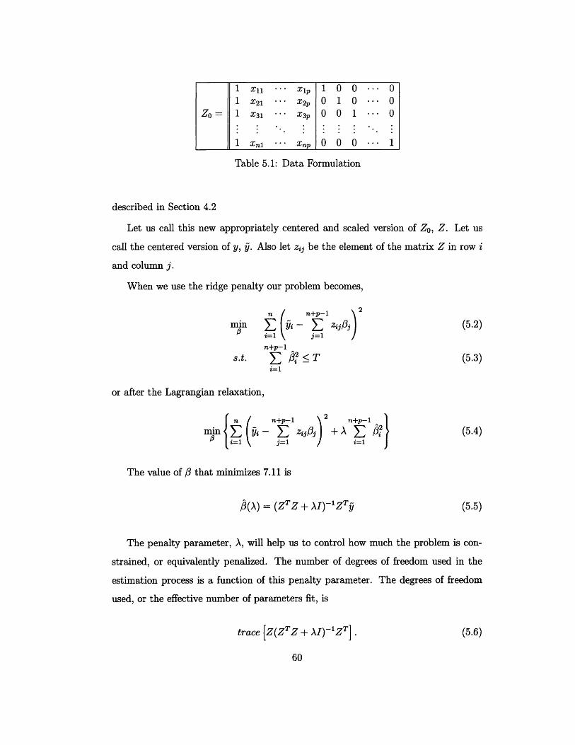
1 Xll ... X1P 1 0 0 *- 01 x2 1 .. X2p 0 1 0 .. O0
Zo = 1 X3 1 x' X 3p 0 0 1 ... 0
1 Xnl ... np 0 0 0 ... 1
Table 5.1: Data Formulation
described in Section 4.2
Let us call this new appropriately centered and scaled version of Zo, Z. Let us
call the centered version of y, y. Also let zij be the element of the matrix Z in row i
and column j.
When we use the ridge penalty our problem becomes,
n n+p-1 2min iE i- E ,jpj)3(5.2)
n+p-1s.t. E 2 T (5.3)
i=l
or after the Lagrangian relaxation,
n+p-1 2 n+p-1
min Yi- z zip3) + > i2 (5.4)1 i=1
The value of P that minimizes 7.11 is
/3(A) = (ZTZ + AI)-zT (5.5)
The penalty parameter, A, will help us to control how much the problem is con-
strained, or equivalently penalized. The number of degrees of freedom used in the
estimation process is a function of this penalty parameter. The degrees of freedom
used, or the effective number of parameters fit, is
trace [Z(ZTZ + AI)-1ZT] . (5.6)
60
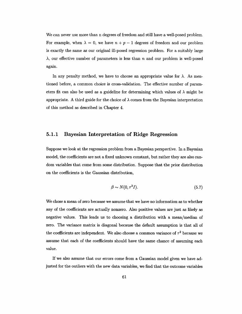
We can never use more than n degrees of freedom and still have a well-posed problem.
For example, when A = 0, we have n + p - 1 degrees of freedom and our problem
is exactly the same as our original ill-posed regression problem. For a suitably large
A, our effective number of parameters is less than n and our problem is well-posed
again.
In any penalty method, we have to choose an appropriate value for A. As men-
tioned before, a common choice is cross-validation. The effective number of param-
eters fit can also be used as a guideline for determining which values of A might be
appropriate. A third guide for the choice of A comes from the Bayesian interpretation
of this method as described in Chapter 4.
5.1.1 Bayesian Interpretation of Ridge Regression
Suppose we look at the regression problem from a Bayesian perspective. In a Bayesian
model, the coefficients are not a fixed unknown constant, but rather they are also ran-
dom variables that come from some distribution. Suppose that the prior distribution
on the coefficients is the Gaussian distribution,
P - N(O, -2I). (5.7)
We chose a mean of zero because we assume that we have no information as to whether
any of the coefficients are actually nonzero. Also positive values are just as likely as
negative values. This leads us to choosing a distribution with a mean/median of
zero. The variance matrix is diagonal because the default assumption is that all of
the coefficients are independent. We also choose a common variance of T 2 because we
assume that each of the coefficients should have the same chance of assuming each
value.
If we also assume that our errors come from a Gaussian model given we have ad-
justed for the outliers with the new data variables, we find that the outcome variables
61
have the following distribution,
Y - N(Z3, 21I). (5.8)
In a Bayesian model, we are interested in calculating the posterior distribution for
the coefficients given the information we get about the coefficients from the data.
Using Bayes Formula,
P(BIA) = P(AIBj)P(Bj) _ P(AIBj)P(Bj)P(A) Ek P(AIBk)P(Bk)
we get that the posterior distribution on the coefficients is,
f(/ly) = f(Y )f(/3) (5.10)f(Y)
(5.11)f f(IPf')f(f')d3'N(y; = Zp, E = a2I)N(P; = , E = Tr21)
f N(ZP, a2I)N(P; = O, E = 721)K exp (8 -Z) T (Z)- p2.Tp (5.13)
where K is a constant, which we could calculate, but it turns out that this is not
necessary.
This is the posterior distribution for /. Now in order to find a point estimate
for A, one popular idea is to use either the mean or the mode of this distribution.
In this example, the mean and the mode are the same value. This is because the
Normal distribution is the conjugate prior for the Normal distribution, i.e. when you
use a Normal prior with data from a Normal distribution, you get a Normal posterior
distribution [12].
We can then just maximize this function to get the mode/mean. It is equivalent
(and easier) to work with the log of the function,
log(f(/3)) = K' + (-- ( - Z)T( - Z/) --3T)) (5.14)2a2 2-r5
62

Now if we differentiate with respect to ,
log(f ()) -1 (2ZTy - 2ZT Z/) + (2) (5.15)
zTZ I _ a y(5.16)a T a
02= (ZT Z + I) _ Ty (5.17)
If we set, this to zero to find the maximum and then solve for /, we get
/3 = (ZTZ + I)-1ZTy (5.18)
This is exactly the solution that we get when we solve a ridge regression problem
if we set A = 2, or we choose the penalty parameter to be the ratio of the error
variance of the data to the prior variance of the coefficients.
5.1.2 Selection
Now let's suppose one has selected a value for A. We still need to do some more work
before you can definitively select variables and detect outliers. The problem here is
the ridge penalty itself. This penalty function does not fit any of the coefficients to
be zero, i.e. it doesn't deselect any of the variables or tell us that any of the points
are not outliers. This feature is due to the shape of the penalty function.
When we view the penalty function as a constraint function, we see that these
estimation procedures should give us the answer where the elliptical contours of the
residual sum of squares first hits the constraint region. The shape of the constraint
function will affect where these contours first hit the constraint region. The ridge
constraint forms a hypersphere. There are no edges or vertices on this type of con-
straint. This means that the optimal values within this constraint are almost always
likely to occur at points where all of the coefficients are nonzero.
In order to remedy this situation, Morgenthaler et. al. choose to examine the
63
ridge t-statistics of the coefficients. They are calculated as follows
tj(A) = /3 (A))&V/(ZTZ + AI)-iZTZ(ZTZ + AI) (5.19)
with 6& estimated robustly by the MAD of the residuals
& = 1.483medyi - z/3(A) - medl~I - zfTl(A)II. (5.20)
Now when Itj(A)l is greater than a certain threshold, we can say that we believe this
coefficient is significantly different from zero. If the index j corresponds to one of
the original variables, we say that this variable should be selected. If the index j
corresponds to one of the data variables, we say that this point is a suspected outlier.
Determining the proper threshold here is very important. Morgenthaler et. al.
suggest the value of two, although they also mention that one could use the effective
number of degrees of freedom to determine a different, perhaps better value, by using
the t distribution . In practice they found that this simple method worked well for
cases without gross outliers and leverage points.
However the simple algorithm experiences problems when there were leverage
points and/or gross outliers. Gross outliers and bad leverage points have the largest
errors and thus should have very large coefficients for their data variables. These large
coefficients make up a large part of the penalty function or constraint for any given
penalty parameter and this interferes with the coefficient sizes of the real variables
and thus our measurements of their significance.
5.1.3 The Pen Algorithm
Morgenthaler et. al. suggest the following five step algorithm to fix this problem.
1. The solution to the optimization problem 7.11 is found using robust (MAD)
ten-fold cross-validation to determine A.
64

2. All rows with"data" variables having Itl > 2 are removed. This step is intended
to remove some of the very large outliers, which were causing problems in the
simple algorithm.
3. The model is again optimized without these rows and a new value for is found
by cross-validation, which we call A*. This is considered to be a "robust" value
of A because it was the one calculated for a cleaner set of the data. A* can be
viewed as a good measure of the ratio 2 from equation 5.18 for a clean data
set.
4. All the rows are again used to optimize 7.11 with A fixed at A*. Rows with
"data" variables having Itl > 4 are removed in this step. The idea here is that
we would only remove those points that seem to be the grossest outliers, when
we are using a good penalty parameter. Removing these points is equivalent to
solving the ridge problem with all the data, but we would allow the coefficients
from these points to be fit free of a penalty. Another equivalent way to view it
is that we model the coefficients corresponding to these points as coming from
a prior with a different Normal distribution that has a variance approaching
infinity (i.e. any error size is as likely as any other).
5. The optimization problem 7.11 is now solved for the remaining rows (i.e. with
all rows, but the ones removed in step 4) with a new A again found by cross-
validation. Explanatory variable selection is done using Itl > 2 as the selection
criterion. This threshold is somewhat low considering the fact that we are
testing multiple hypothesis, but in some ways it may be desired to be more
cautious in removing variables, than in keeping them around.
We will examine the performance of this algorithm in Chapter 6. The results of
the Morgenthaler et. al. paper indicate that this algorithm has a weakness when it
comes to data sets with leverage points. Our first improvement to their algorithm
attempts to address this problem.
65

5.2 Non-equivalence in Priors
As mentioned before, these penalty methods easily can be interpreted in a Bayesian
context. In standard ridge regression, we assume that each of the variables are just as
likely to be in the model (because we are using a common prior mean and variance)
and that, in general, we believe that there is no evidence that any of the variables
should be in the model (we assume a prior mean coefficient value of zero). In the
absence of information this makes sense.
Often we do have some information about the importance of variables or the
outlyingness of data points. We could get value from incorporating this information
into our calculations. Suppose we have some prior belief that a coefficient is non-
zero. It would not make sense to then choose a prior that is zero mean with the same
variance as the other variables. It might make more sense to choose a prior that has
some non-zero mean value or one that has a larger variance.
Assuming our nonzero prior estimate for 3 is somewhat accurate, we will end up
with better posterior estimates. In order to get an accurate estimate we need to
use an estimation method to find this nonzero mean value that is less sensitive to
leverage points. This will protect us against the problems that the original algorithm
had with leverage points. Another way is to find a prior guess that had a better
predictive ability (under a robust prediction measure) than using all zero coefficients.
Another benefit to using a nonzero mean prior in this algorithm is that it allows
the original variable coefficients to only contribute to the constraint term by how much
they differ from our prior and not by how much they differ from zero. Assuming our
nonzero prior estimate for 3 is somewhat accurate, we will leave plenty of room in the
constraint to fit any unusually large coefficients on the "data" variables corresponding
to outliers.
As mentioned before, when we have even just one very large outlier we can ex-
tremely over-penalize the original variables by using equivalent zero mean prior for
all of the variables. This is readily apparent when we look at the problem in the
constrained minimization context. If we want J(/3) = En+p 2 < U then if one of the
66

pi is very large the others have to be small so that the sum of their squared values
remains less than U.
One way to get prior information about the coefficients is to get a crude estimate
from a small sample of the data. If we can find a set of coefficients that have a
suitable predictive ability (under a robust prediction measure) then we can have some
confidence in those values as useful prior information, for when we consider the whole
data set. Using a small sample also helps us when it comes to the leverage points. As
described in Chapter 3, sampling-based methods are some of the few effective ways
to deal with leverage points.
5.2.1 The Nonzero Mean Prior (NZMP) Pen Algorithm
In this subsection, we will describe the algorithm that we developed around this idea.
1. The first phase of the algorithm involves sampling to get a good approximation
of the coefficients to use in the mean value for our prior. We take a random
sample (without replacement) s of size p of the indices 1... n}. The s refers
to the fact that it is a sample and the I is the index of the sample, because
we are taking more than one. Let v (v for validation) be the sample of indices
that is the complement of sI. Let Xs, and y,,s be the sample of the rows of the
centered and scaled versions of X and y. Also let the rest of the data be called
X,, and Y,, respectively (v is for validation).
Then we create a new matrix Z,, by augmenting Xs, with the first p or p - 1
columns of a p x p identity matrix, just as in the Pen Algorithm [45]. Including
all p columns would allow one new variable for each data point included in the
sample, as desired. Initially because of our concerns about multicollinearity
with the intercept term, we decided to not include one of the data dummy
variables. This choice was random. Later, we realized that including all p did
not cause sufficient problems to force us to leave one dummy data variable out.
We make note of the choice to use p - 1 however because that was the value we
used in our simulations described in Chapter 6.
67
For the purposes of the following algorithm description we will add data dummy
variables for all but one of the data points. The point that is not included will
be randomly chosen.
Then we then find /(A) (for a range of A's) that solve the following equation:
( n 2p-1 \ 2 l2p-1/1I(A) = arg min { Ys,i - E ZsI,jk 3k)+ E ) (5.21)
j=l k=l k=l
For each /3(A), a prediction score based on how well the first p components of
this estimate of /3, p/3(A), can be used to predict the results based on the obser-
vations we left out in the validation set. p(A) corresponds to the coefficients
on the original p variables.
We then calculate the residuals corresponding to using the coefficients pI(A),
RA,I = y,, - X., (pi(A)). (5.22)
We then calculate the following robust prediction score,
PS,,I = median {I[R,] - median(R,,I)) (5.23)
We repeat this procedure for a large number of different samples. (In our
simulations which will be described in Chapter 6, we chose 100 and this value
worked well. For other sets this value may need to be increased, to allow us
to consider a sufficient number of samples.) Then we choose X = pp* .(A*) for
which A*, I* = arg minx,({PS,I}.
Now, 3, is the estimate of 3 associated with the smallest MAD score of pre-
diction residuals and we use this as our best prior guess for beta. Note, we are
only finding non-zero priors for the original variables and not the data variables.
The data variables will continue to have zero priors.
2. Then we again split the whole centered and scaled data set randomly into a
68
training set of size nc and a validation set of size n, = n - n. In the process
we create the data sets, Xc8, Ycs, Xvs, Yvs. We do this for 30 random splits of the
data, s E 1,..., 30. As before, we augment the training set, X,, with the data
dummy variables to create the new matrix, Zc,. Let Zc.,ij be the element of the
matrix Z,, that is in the ith row and jth column.
We then solve the following,
3c,(A) = argmmin {ycAsi- cs - c,ij(±j) + A ( 1-ir,)2 J(A) n+p-- 1 Z n~--i
= argmin {(yc, - Z3) (y, -Zc) + A( - ,) (3 - 3)}
We find the maximizer by differentiating with respect to P and setting this equal
to zero. (We will not show the second derivative here, but it is a maximum.)
-2ZT(yC - Zcfs) - 2AI( - fi) = 0 = (5.24)
(ZrCZc. + AI)3 = (Zcsyc + AI3) = (5.25)
c3,(A) = (zcZ, + ±AI)- (ZYc + AI3r) (5.26)
We do this for 30 random splits of the data and over a range of A. (We did not
see improvements in our simulations from using more than 30 iterations.)
For each random split, we calculate the prediction residuals again only with the
first p coefficients (the other coefficients do not make any sense with a different
data set). Let us call these coefficients pc, (A).
RA, = Y - X,, (pci, (A)). (5.27)
We then calculate and save a matrix of values corresponding to the following
robust prediction score (MAD),
PS, = median ({[Rx,] - median(Rx,)I} (5.28)
69
For each A, we take the median of the prediction score over the 30 samples.
PS(A) = median,(PSx,,) (5.29)
This value is seen as a robust measurement of the predictive ability associ-
ated with this value of A. We then chose A* equal the A corresponding to the
argument minimizer of these medians,
A* = arg min PS(A) (5.30)
3. We then use the A* calculated in step 2 to find estimates of the coefficients using
the full data set, using a ridge penalty with our prior guess A,.
(·>) = (ZTZ + AI)-l(ZTy + AI) (5.31)
We then calculate t-statistics for the columns associated with the data points.
In order to calculate the t-statistics, we need to calculate the variance matrix
of the coefficient estimates.
This is difficult because we do not know the distribution of/ 3. We could do some
sort of bootstrap estimate, but this would increase the computational intensity
of our algorithm. Instead, we assume that 3 is a constant. This assumption
is not too far-fetched because the estimation method for X, is rather crude and
most of the values (n of n + p) are constants (zeros). Additionally, in this step,
we are mainly interested in finding the t-statistics for the dummy data variables
and these are the ones with constant values in A,.
Given this assumption, we end up approximating that the variance is the same
as the variance associated with a standard ridge regression.
Var[(A*)] = Var[(ZT Z + A*I)-i(ZTy + A*I,)] (5.32)
- Var[(ZTZ + A*I)-lZTy + const.] (5.33)
70

o U2(ZTZ + A*I)-ZTZ(ZTZ + XA*I)-
We use this to get approximate t-statistics,
t(j(A*)) 3= j(A*) (5.35)a6[Var(3(A*))]j
We remove any data points that have corresponding t-statistics of 2 or more.
These data points correspond to points that we believe are highly likely to be
outliers.
Note, that we still need to remove points in this algorithm even though we
adjusted the priors. This is because large outliers still end up being a problem.
The new means for the priors are not exact and we still need to allow the
algorithm to choose values for the coefficients that are possibly very different
from these "best guesses".
4. Repeat step 2 on the remaining data left after removing some outliers in step
3. Repeat step 3, except now we remove points with t-statistics of 2.5 or larger.
Do not leave less than 1.25p points remaining. This is because in the next
step we will be performing a five-fold cross-validation and otherwise we would
not have enough points in the training set. If the algorithm wants to take out
more, leave the 1.25p points with the smallest t-stats. (Note: Two passes at
removing outliers were used here because very large outliers would overwhelm
the algorithm, making other less serious outliers seem like they were not outliers
at all.)
5. We assume we now have a "clean" data set without any outliers. Let us call
this data Xciean and Yean. We add dummy data variables to create ZO,dean.
We then create Zdean from ZO,clean by appropriately centering and scaling the
variables. We also robustly center Yclean to create Ylean.
We then fit this data with the original ridge penalty (i.e. use the zero prior)
as in the minimization 7.11 using a five-fold cross-validation to choose A. We
71
(5.34)
choose A, corresponding to the A with the smallest sum of squared prediction
scores across the five groups.
6. We now consider the solution to the ridge regression problem with Zcean and
Yclean to be,
/ = arg min {i (Ycean,i- A Zclean,ijj) + A* ( ) } (5.36)
7. Calculate t-statistics for the original variables using the formula 5.19. If the
t-statistic is higher than T, count the variable as having been selected, where
T is appropriately chosen to balance out false positives and false negatives.
Note: When considering A's we never used very small A's due to the fact the
effective number of parameters we fit would be to high and we would have
problems with degrees of freedom.
5.3 LASSO and LARS
In this section we will consider an different kind of penalty function than the ridge
one. This other alternative for our penalty function is,
n+p
J(3) = I311I. (5.37)1=1
This penalty function corresponds to what is known as LASSO penalty [61], in the
statistics literature. LASSO stands for Least Absolute Shrinkage and Selection Op-
erator.
As is suggested in the name, this penalty function was originally created because
it was believed that it would be useful for selection. This is due to the fact that
unlike the ridge penalty this penalty will often give us zeros for the fitted coefficients,
indicating that a variable should not be selected. This feature is again due to the
shape of the penalty function.
72
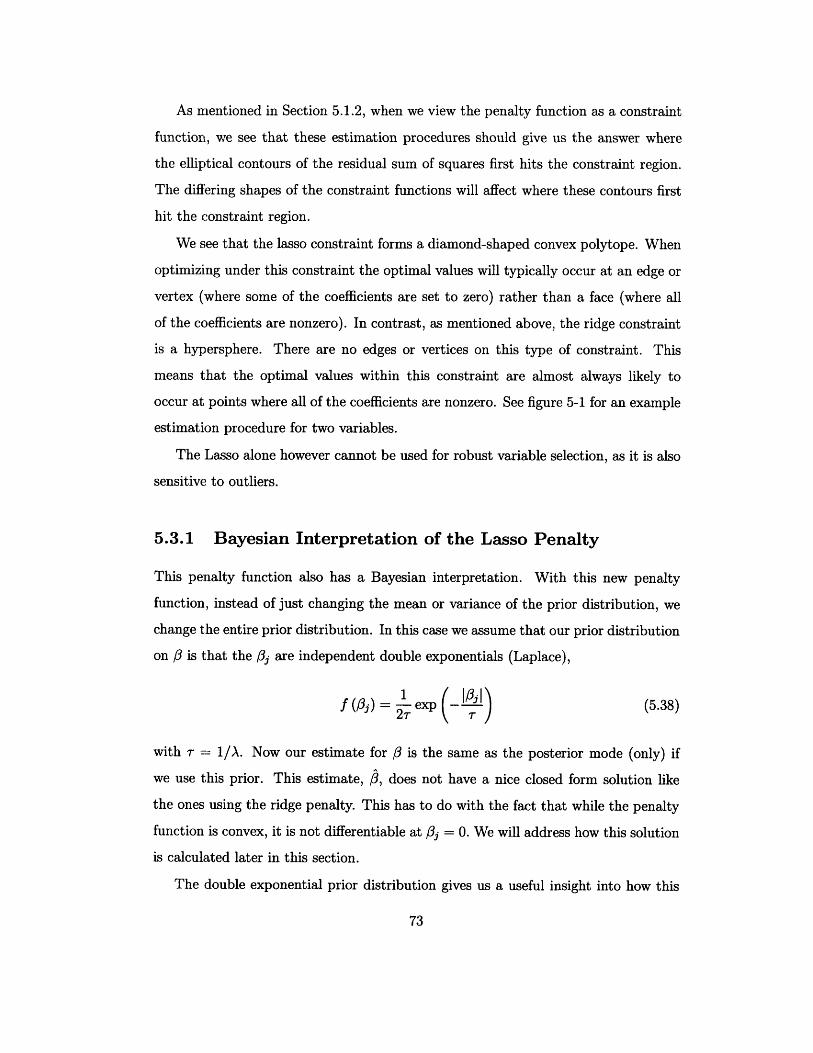
As mentioned in Section 5.1.2, when we view the penalty function as a constraint
function, we see that these estimation procedures should give us the answer where
the elliptical contours of the residual sum of squares first hits the constraint region.
The differing shapes of the constraint functions will affect where these contours first
hit the constraint region.
We see that the lasso constraint forms a diamond-shaped convex polytope. When
optimizing under this constraint the optimal values will typically occur at an edge or
vertex (where some of the coefficients are set to zero) rather than a face (where all
of the coefficients are nonzero). In contrast, as mentioned above, the ridge constraint
is a hypersphere. There are no edges or vertices on this type of constraint. This
means that the optimal values within this constraint are almost always likely to
occur at points where all of the coefficients are nonzero. See figure 5-1 for an example
estimation procedure for two variables.
The Lasso alone however cannot be used for robust variable selection, as it is also
sensitive to outliers.
5.3.1 Bayesian Interpretation of the Lasso Penalty
This penalty function also has a Bayesian interpretation. With this new penalty
function, instead of just changing the mean or variance of the prior distribution, we
change the entire prior distribution. In this case we assume that our prior distribution
on is that the j are independent double exponentials (Laplace),
f (j) = 1 exp ) (5.38)
with -r = 1/A. Now our estimate for is the same as the posterior mode (only) if
we use this prior. This estimate, /, does not have a nice closed form solution like
the ones using the ridge penalty. This has to do with the fact that while the penalty
function is convex, it is not differentiable at /3j = 0. We will address how this solution
is calculated later in this section.
The double exponential prior distribution gives us a useful insight into how this
73
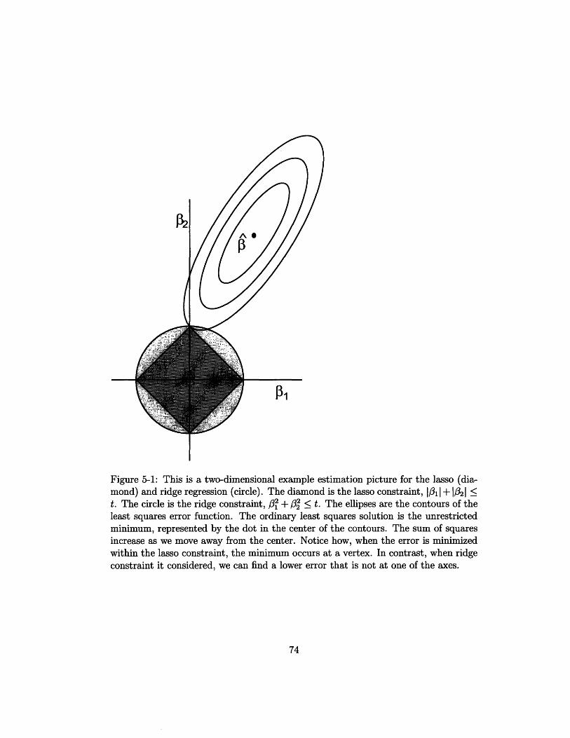
P2
!
P1
Figure 5-1: This is a two-dimensional example estimation picture for the lasso (dia-mond) and ridge regression (circle). The diamond is the lasso constraint, 1i1 I + 121 <t. The circle is the ridge constraint, 32 + /3_ < t. The ellipses are the contours of theleast squares error function. The ordinary least squares solution is the unrestrictedminimum, represented by the dot in the center of the contours. The sum of squaresincrease as we move away from the center. Notice how, when the error is minimizedwithin the lasso constraint, the minimum occurs at a vertex. In contrast, when ridgeconstraint it considered, we can find a lower error that is not at one of the axes.
74
U.5
0.45
0.4
0.35
0.3
0.25
0.2
0.15
0.1
0.05
N
-4 -3 -2 -1 0 1 2 3 4
Figure 5-2: This figure shows the differences in shape between the normal (prior forridge) and double exponential (prior for LASSO) distributions.
type of penalty method should work. This prior puts both more density at zero and
more in the tails, than the normal distribution (see Figure 5-2). This corresponds
well to our belief that the coefficient should either be zero or something significantly
nonzero. We are not as much interested in the values in between. The increased
density in the tails should help is with the problems we were having with the gross
outliers.
5.3.2 Benefits of LASSO Over Ridge
There are several benefits of using the LASSO penalty instead of a ridge penalty.
When using the LASSO we have the benefit that coefficients are often set to zero,
whereas when using a ridge penalty the coefficients are almost never chosen to be
zeros. In the absence of hard zeros, we are left with the problem of determining when
a small coefficient is small enough to be insignificant. This adds another parameter
and more complications to such an algorithm.
We no longer have to worry about using t-statistics in the intermediate stages of
our algorithm. In fact as A decreases, we only are only interested in the ordering in
which the coefficients are set to a non-zero value. We can use this to determine which
75
A -
variables are most important for our model because they were included even under
the strictest penalties.
We must note that, the LARS ordering of the variables is not the only measure
of the importance of the variables. t-statistics can still be useful because sometimes
variables with small and insignificant coefficients can be added to the model before
other variables with larger and significant coefficients.
Additionally the LASSO is known to out perform the ridge when we are looking
for a "small to moderate number of moderate-sized effects" or a "small number of
large effects" [61]. In our case we expect that a large portion of the coefficients should
be zero (corresponding to original variables that do not belong in the model and data
variables that do not correspond to outliers) and that all of the rest (true original
variables and outlier data variables) should have moderate to large effects.
One original drawback of the LASSO was that the coefficients were somewhat
difficult to compute. Unlike the ridge coefficients with their closed-form solution, for
the LASSO the original solution methods involved solving a quadratic program. This
was a computationally intensive method, until the Efron et. al. developed Least Angle
Regression (LARS) [14] (see also Chapter 3). They showed how a simple modification
of the LARS algorithm can be used to calculate all possible LASSO estimates. Using
the LARS algorithm means that computations using the LASSO penalty should be
faster than computations using the ridge penalty.
5.3.3 Least Angle Regression: A Close Relative of LASSO
Efron et. al. [14] boast that the LARS algorithm can be used to compute all pos-
sible Lasso estimates an "order of magnitude times faster than previous methods."
The ordinary LARS algorithm (before the LASSO modification) requires only the
computational effort of ordinary least squares applied to the full set of variables.
The standard LARS algorithm will not give us LASSO solutions. Let be a Lasso
solution, with g = Xf. In Lemma 8 of Section 5 of [14], it is proven that, the sign
of any nonzero coordinate j must agree with the sign sj of the current correlation
cj = xjT(y - ), that is sign(^j)= sign(j)=sj. The standard LARS algorithm does
76

not enforce this restriction, but can be modified to do so.
Basically the modification enforces that when we take our step along the equian-
gular direction, that we never take a step large enough such that we violate this
constraint. Instead we take the largest such step that doesn't violate this constraint.
This will set one of the current nonzero coefficients to zero and this variable will be re-
moved from the "active" set. This turns out to be a major distinction between LARS
and LASSO; LARS always adds a new variable each step, but in LASSO variables
can enter and leave the active set.
Theorem 1 in [14] states "Under the Lasso modification, and assuming the 'one
at a time' condition discussed below, the LARS algorithm yields all Lasso solutions."
The proof of this theorem and all of the mathematical details of the Lasso modification
can be found in [14].
As Efron et. al. [14] mention in their paper, "LARS is interesting in its own right."
Despite the fact that Least Angle Regression is not explicitly a penalty method, we
will consider it a similar alternative to the penalty methods. Knight [35] suggests
that the objective functions of Stagewise and LARS may be similar to the objective
function of the LASSO. He suggests a possible way to construct an implied objective
function, but doesn't follow the idea through. This is an interesting aside, but is
somewhat beyond the scope of this thesis.
5.3.4 The Simple dLASSO/dLARS Pen Algorithm
In this section we will describe a new penalty algorithm that we have developed
around the LASSO penalty and LARS algorithm. The LASSO penalty leads us to
the following minimization problem,
n n+p-1 2 n+p-1min Yi- zij)j + A E /ai (5.39)
i=1 j=1 i=1
where y and zij are defined as they were in the previous section.
1. We start by robustly centering and scaling the explanatory data matrix, X, and
77

augmenting this original data set with a centered version of the identity matrix
as in the previous sections, to form the Z matrix. We also center the outcome
variable to form y.
2. We then use the LARS algorithm with the LASSO modification (although we
will find that the LARS algorithm works well here even without the LASSO
modification) to solve the full path of 5.39 for all values of A. We are primarily
interested in determining the order in which the original variables and data
variables become nonzero, which corresponds to the order in which they are
added into the model.
3. We consider the models in order as we reduce the penalty parameter, A, from
infinity to zero. We then take the first model with m variables, where m is
a parameter of the algorithm. We then fit coefficients on these m variables
using ordinary least squares. These may not be the first m variables to enter
the model, because in the case of the LASSO penalty, sometimes variables will
leave the model after having entered. These m variables might include both
some of the original variables and some of the data variables. The number m
is determined by n (the number of data variables), p (the number of original
variables), and the percentage of contamination suspected to be in the data set.
A suggested value we considered for simulations was m = p + .25n.
The idea behind this value is that it is a possible upper bound on the number of
nonzero parameters that we would want to fit assuming there is 25% contami-
nation in the data. We would then want to fit at most one variable for each of
the p original variables plus one for each of the outliers, which on average there
would be .25n of them if there is 25% contamination.
4. Given that in the last step we probably chose too many variables, we need to
narrow this set down to just the significant ones. In this step, we calculate
t-statistics on the "real" variables from the ordinary least squares calculation of
step 3. If the t-statistic corresponding to a given variable's coefficient is larger
78

than our cutoff value, T, then we have determined it is significant and this
belongs in the model.
The choice of T is determined by both the amount of Type I error we are
interested in having and the number of such tests we are performing. When
performing multiple comparisons we have to take into account that treating the
tests as independent is incorrect. For ease of calculation we can use a Bonferroni
approximation here.
Variant of the dLASSO/dLARS Simple Algorithm
In step 4 described above, we perform a test on the original variables to determine
whether or not they should be included in the model. We did not however perform
a step where we narrowed down the number of data variables that we considered.
One could consider performing the similar test on the data variables, in which an
insignificant result would indicate that there is not enough evidence in the data to
state that this point is an outlier. Then perhaps this data variable should not be
considered in the step where we test the significance of the original variables.
This algorithm would be the same as the LASSO/LARS Simple algorithm, except
we would add another step before the last step. In this new step, we are going
to narrow the set down by removing some of the data variables before we test the
significance of the real variables.
We calculate t-statistics on the data variables from the ordinary least squares
calculation of step 3. If the t-statistic corresponding to a given variable's coefficient
is smaller than our cutoff value, Td, then we have not determined it is significant, so
we remove it from the model. The choice of Td is determined by both the amount
of Type I error we are interested in having and the number of such tests we are
performing (i.e. the number of dummies selected by the Lasso(LARS) step). For ease
of calculation we use a Bonferroni approximation here.
Now that we have removed some of the data variables, we perform the last step
as described above to figure out which of the real variables are significant. Hopefully
in the previous step we have removed some of the data variables allowing this second
79

calculation to have more degrees of freedom.
5.3.5 The Sample dLASSO/dLARS Pen Algorithm
In the last subsection, we described a simple algorithm that used the LARS algorithm
(either the LASSO penalty or the Least Angle Regression versions) to select the
variables and outliers from the original variables and the data variables. We will
see in Chapter 6 that is algorithm performs rather well in many cases. We still are
interested in improving it. One idea to improve this basic algorithm is to try to
somehow include the idea of bagging [11] in a new version of it. Consult Section 3.3.3,
[11], or [9] for a description of bagging.
The sampling method we describe here is very similar to bagging, but has one
main difference. We do not use sampling with replacement to get a sample of size
n as in a standard bootstrap. Instead, we choose, without replacement, a large, but
smaller than size n, sample from the data set. We sample without replacement to
avoid the complications involved with adding the dummies for the data points which
were selected more than once.
Initially we considered large sample sizes, like 2, in order to closely replicate the
full sample and in order to maintain a larger number of degrees of freedom for the t-
statistic calculations we make. Later we also considered smaller samples closer to the
size of the elemental sets because of the robustness properties of using such sets. The
difficultly here is choosing a small set while still having enough degrees of freedom to
get good results from the t-statistics.
Unlike in the sampling-only algorithms described in Chapter 3, we are not re-
lying on small sample sizes alone to achieve robustness. The dummy variables we
added for the data points were designed to provide us with a more robust ordering
of the variables from the LASSO/LARS procedures and a robust measure of the t-
statistics of the original variables. We found that this is true in our simulations of
dLARS/dLASSO Simple (see Chapter 6). So if the method works well enough for
the full data set (as in dLARS/dLASSO Simple), there is no evidence that we need
smaller sample sizes. Although we must recognize that the dummies are technically
80

only designed to help us with additive outliers, so leverage points may still cause us
some trouble with these large sample sizes.
With any choice of sample size, the algorithm should proceed in a similar way.
We will now describe our sampling version of dLARS/dLASSO Simple, which we call
dLARS/dL,ASSO Sample
dLARS/dLASSO Sample Algorithm
1. Appropriately center and scale the original data set as in our previous algo-
rithms.
2. Choose a sample of size ns from the data set. Add the appropriately centered
dummy variables for the selected data points.
3. Run the LARS algorithm on this new data set. Select the m variables that
appear in the first model with m variables, original and data, which come out
of the algorithm. We suggest choosing m = p + Kn,, where K is the fraction of
contamination that you expect in the data set. As for K, many robust regression
tools choose a default of K = .25.
Once again, as in Simple dLARS/dLASSO, this choice is an upper bound on
the number of nonzero parameters that we would want to fit assuming there
the fraction of contamination in the data is K.
4. Once again, the previous step may have overestimated the number of variables
we should select. Fit an OLS regression with this reduced set of m original and
data variables. Calculate t-statistics associated with the coefficient estimates
for each of the variables.
5. Choose an original variable for inclusion in this sample's final model if it has a
corresponding t-statistic larger than our cutoff value, T. (Note: we could have
used the Simple dLARS/dLASSO variant here, in which case there would be
another two steps added.)
81

The choice of T is determined by both the amount of Type I error we are
interested in having and the number of such tests we are performing. When
performing multiple comparisons we have to take into account that treating the
tests as independent is incorrect. For ease of calculation we can use a Bonferroni
approximation here.
6. We repeat steps 1 - 5 S times, where S is a large number. From here there are
multiple ways of creating the final model from these S different sample models.
A. Choose the final model using a a similar method of determining the final
model to the one used in LARS Draws. We count the number of times a given
variable appears. If it appears more than a certain threshold number of times,
it is selected for the final model. Bagging [11] suggests that we choose the cutoff
of 50% here because we should classify things to the side with the most votes.
B. This choice is a variant of choice A in which the different models are weighted
by their predictive ability. We use the coefficients in each OLS regression to
predict the values of the out of sample set. We then calculate a robust prediction
score based on the residuals from our predictions. Given that a lower score is
more desirable for most prediction scores we consider, we weight the different
models by the normalized inverse of the prediction score. We normalize these
inverses, so that the total sum of the weights is 1. We then proceed as in choice
A and total up the weighted sum of the times a variable appears. If this score
is more than 50% we select this variable for the final model.
C. Choose the final model as the model that shows up the most among the S
different sample models.
5.3.6 dLARS Draws
One can come up with another type of dLARS (LARS with data dummies) sampling
algorithm, which combines dLARS with the ideas of LARS Draws. Basically the idea
is that instead of using LARS to determine the models we consider in the Draws
algorithm, we use dLARS. By adding dummies for the samples, we are possibly
82

allowing for more of the "bad" samples to give us better measures of the model
statistics.
There are actually two ways of viewing this algorithm. One is as we described
it above, a variant of the LARS Draws algorithm. The other is just as a dLARS
sampling algorithm which uses cross-validation to choose the appropriate stopping
points of the dLARS algorithm.
The dLARS Draws Algorithm
1. Take a sample from the rows of the data of size, n, where n > p. In fact,
we recommend choosing a sample of size n > 4, in order to accommodate
an average of 25% outlier contamination any sample. We add dummy data
variables for each point and we appropriately scale and center the columns as
recommended in our previous algorithms. Now we have p + n8 variables to
choose from and the LARS algorithm will fit n, different sets of coefficients.
Some models may have the same exact real variables, but will have different
sets of data variables. These cases will occur whenever one of the data variables
is chosen to join the set of non-zero coefficients. This means that some of the
real variable models will be represented more than once, except with a different
set of values for the LARS coefficients.
2. Save the LARS coefficients for each of the n steps of the LARS algorithm.
Calculate a robust predictions score associated with each of the n8 models. One
choice for the robust prediction score is the MAD of the residuals found from
predicting the out of sample data with the LARS coefficients.
One could also calculate the OLS coefficients associated with fitting each of the
n8 models on this sample, as is suggested in the LARS-OLS hybrid method in
[14]. In this case, we can calculate a robust predictions score associated with
each model, for both sets of coefficients (LARS and OLS). We will save the
better (lower in the case of MAD) of the two scores and call this the "combo"
83

prediction score. In LARS Draws, we found in our simulations that choosing
the "combo" prediction score lead to better overall results than using either of
the two scores exclusively. This is not the case for dLARS Draws, in this case
using the combo prediction score doesn't give us appreciably different results
from using the LARS prediction score. We will address this in more detail in
Chapter 6 when we evaluate the performance of our algorithms.
3. We repeat steps 1 and 2 for a large number of samples M and save the n8 models
and n8 robust prediction scores from each sample.
4. We will now proceed as in the Draws and LARS Draws algorithms by ranking
the models by their robust prediction scores. We will get rid of the models with
the worst prediction scores. In the case of our simulations, we considered the
best models to be those with the prediction scores equal to or below the first
percentile.
5. Then among these best models, we sum up the number of times each variable
appears. If a variable appears more than a certain threshold value, we determine
that it belongs in the final model.
Many of the same concerns about parameter choices exist here as they did in Draws
and LARS Draws. See Chapter 3 for a discussion on parameter choice. The main
difference in this case is that we recommend choosing a larger sample size, n > 4p
If the contamination level of the sample is 25% we would on average expect 2 outliers
in a sample of size 4P. With such a sample size are able to fit the p + .25n8 = 4P3' 3
non-zero coefficients that we would desire according to the arguments described in
the dLARS Simple algorithm.
84

Chapter 6
Evaluating the Algorithms'
Performances
We have presented a number of promising ideas for algorithms, but we still need to
evaluate their performances to determine their usefulness and to compare them to
other methods in the literature. One of the main ways we will evaluate our methods
is to analyze their effectiveness in determining the correct model via a Monte Carlo
simulation. As Breiman stated in reference to demonstrating the usefulness of his
nonnegative garrote method, a penalty method for subset selection, "Because analytic
results are difficult to come by in this area, the major proving ground is testing on
simulated data." [10]
Sauerbrei [56] points out that "comparisons of selection strategies are usually made
on specific data sets or by using simulation." Examples of such work are Roecker 1991,
Breiman 1992 and Sauerbrei 1992. Sauerbrei also points out that for methods involv-
ing resampling "simulation studies are promising ways to investigate the possibilities
and limitations because analytical results may be achievable only for parts of the
procedures."
At best, the analytical results we can get are asymptotic results for these parts,
but "with a limited set of data and a large set of models asymptotic results for model
selection will typically no longer apply." [27]
We also find it important to test our algorithms on real data sets, as was also
85
suggested by Sauerbrei [56]. We will compare our results to the commonly held
beliefs on the model composition of those data sets.
6.1 Simulations
Specifically, we will use the Monte Carlo simulation framework proposed by Ronchetti
et. al. [50]. This simulation framework was also used by Agostinelli [1], Morgenthaler
et. al. [45], and Khan et.al. [34]. Using this framework allows us to both test
our method against various error types and to easily compare our algorithms to
the algorithms that are currently in use or being developed because we are using a
common simulation.
Following Ronchetti et. al., we consider four different error distributions, three of
which represent various deviations from normality. The first error case we consider
is the standard normal (Normal(0,1)), which we call el. It is important to consider
a non-contaminated 0 mean, constant variance normal error distribution in order to
show that the method will still work at some sufficient level given data generated
under the standard regression model.
The next three error distributions are labelled as follows: e2 is 7% wild (93%
from a standard normal and 7% from a normal with ,u = 0 and a = 5), e3 is slash
(a standard normal divided by a uniform on (0, 1]), and e4 is 10% asymmetric wild
(90% from a standard normal and 10% from a normal with /u = 30 and a = 1)
These final three error types give us a good sample of the different types of con-
tamination that can be found in a data set. With e2, we have a mixture of Gaussian
type errors. This type gives us a standard Gaussian with slightly more weight in the
tails. e3 is a very heavy-tailed distribution. In this type we could have some very
large outliers and they could be positive or negative effects. In the fourth type our
error is asymmetric, unlike the previous three.
We consider two different simulated design matrices, each with six variables. The
first will entirely be generated from a uniform [0, 1] distribution. The second design
matrix will be generated similarly with the exception that two of the points will be
86
randomly replaced with the value (5, 5, 3, 3, 3, 3) in order to enable us to consider the
possibility of leverage points.
We first consider the case where five of the six coefficient parameters have nonzero
values and the sixth is zero. We chose the coefficient parameter values to be the
size that would generate t statistic values with an average value of 6 under the el
distribution.
We will perform 200 such simulations and we will keep track of how many times
we get the correct result. We might also keep track of the number of times we get an
answer that is close to being correct, e.g. when we are only one variable choice away
from being correct.
6.1.1 Results and Conclusions
The Table 6.1 records the number of times each of the algorithms recorded a correct
result out of 200 trials. We consider a number of different algorithms. Most of them
are robust model selection algorithms, but we have also included some standard model
selection algorithms for comparison.
It is important to recognize that the value in these charts are random variables.
It we were to perform the simulations again, we would get a different set of values.
One could model the number of successes we observe as a binomial random variable,
with some unknown probability, PaLg,om, of success.
In our case, our variance on the observed number of successes is 200 Palg,o(1 -
Palg,om). This means we can have a maximum variance of 50 (or standard deviation of
7.07). We can get a better estimate of the variance by estimating Palg,om as Palg,om =
08,cces0,lom, where successalg,om is the number of successes we observed when using a
given algorithm on our simulated data with a given outlier model. This leads to an
approximate 1 - a confidence interval of [successalg,om , Za/2V200faig,om( 1 - ag,om)]
For example when applying LARS Draws to the simulated data sets with the lever-
age version of the e4 error model, we observed 175 successes in 200 trials. We estimate
the probability of success as PLARSDraws,e4L = .875. This leads to an approximate 95%
confidence interval of [165.83, 184.17].
87
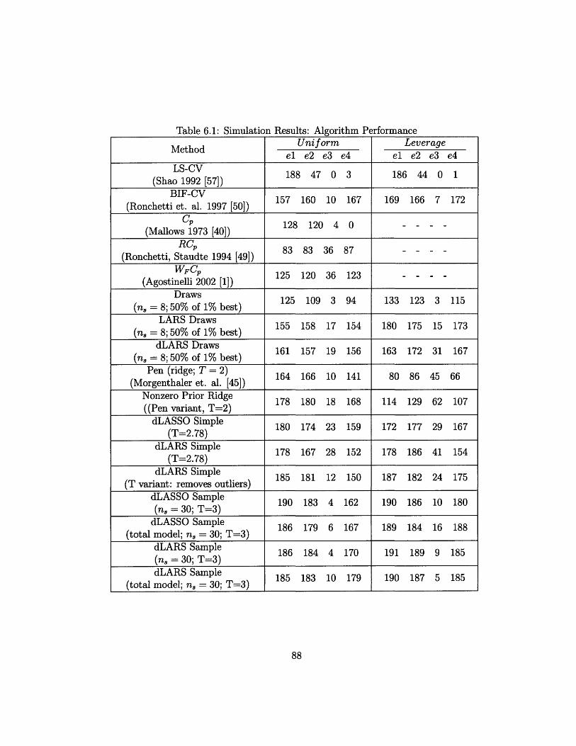
Table 6.1: Simulation Results: Algorithm PerformanceUniform Leverage
el e2 e3 e4 el e2 e3 e4
LS-CVLS-CV 2[5188 47 0 3 186 44 0 1
(Shao 1992 [57])BIF-CVBIF-CV 157 160 10 167 169 166 7 172
(Ronchetti et. al. 1997 [50])Cp
CP 128 120 4 0(Mallows 1973 [40])
RCp 83 83 36 87 ....(Ronchetti, Staudte 1994 [49])
WFcp 125 120 36 123 . ...(Agostinelli 2002 [1])
DrawsDraws 1%bes125 109 3 94 133 123 3 115
(n = 8; 50% of 1% best)LARS Draws(n%LARS Draws 155 158 17 154 180 175 15 173
(n = 8; 50% of 1% best)dLARS Draws(i 8dLARS Draws 161 157 19 156 163 172 31 167
(n = 8; 50% of 1% best)
Pen (ridge; T= 2) 164 166 10 141 80 86 45 66(Morgenthaler et. al. [45])
Nonzero Prior Ridge 178 180 18 168 114 129 62 107((Pen variant, T=2)
dLASSO Simple 180 174 23 159 172 177 29 167(T=2.78)
dLARS Simple 178 167 28 152 178 186 41 154
(T=2.78)dLARS Simple(Tv dLARS Simple u185 181 12 150 187 182 24 175
(T variant: removes outliers)
dLASSO Sample 190 183 4 162 190 186 10 180(n, = 30; T=3)
dLASSO Sample(tdLASSO Sampl e 186 179 6 167 189 184 16 188(total model; n = 30; T=3)
dLARS Sample 186 184 4 170 191 189 9 185(n8 = 30; T=3)
dLARS Sample 185 183 10 179 190 187 5 185(total model; n = 30; T=3)
88

We rnay also be interested in each of algorithms' average performance across the
different; error distributions that we considered. Alternatively, we can also consider a
similar figure where we only average the number of correct models across the normal
mixtures (i.e. we leave out the e3 and e3L slash errors). See these results in Table
6.2.
Conclusions about Other Methods from the Literature
In Tables 6.1 and 6.2, we include simulation results from a number of other methods
from the literature. We feel it is important to compare our methods to them and to
also learn about their weaknesses and strengths.
The first two we would like to analyze are LS-CV [57] and Cp [40]. These are both
methods for solving the standard model selection problem, where we do not have to
worry about outliers or leverage points. Each of them show strong deficiencies when
it comes to handling outliers.
LS-CV performs particularly well in the el case, as expected, with 188 out of 200
correct. Additionally it also does well in the el leverage case with 186 out of 200
correct. LS-CV fails badly if we consider the e2 error types, for both the uniform
and leverage data models, with less than 25% correct in each. This is particularly
disappointing because the e2 error distribution is only a slight modification on the
standard normal error, that has slightly heaver tails. We would hope that our model
selection method would be robust to even small deviations in the error model, but
this one is not. In the e3 and e4 error models, there are practically no correct answers.
In fact, we do worse than one would expect with random guessing.
With Cp we see something slightly different. In the el error model we do not do
as well, with only 128 out of 200 correct. Note though that when using Cp in the
simulation the final model was chosen as the one with the lowest value of Cp such
that Cp < p. This is not the recommended way to use Cp, but it is the way many
people do use it. It is recommended that we consider all models with Cp p or lower.
If Cp is used this way there is no best choice for the model. In the 72 of 200 that we
get incorrect perhaps the correct model is among those with Cp < p, but we would
still have to correctly choose the right answer out of the many models with Cp < p.
89
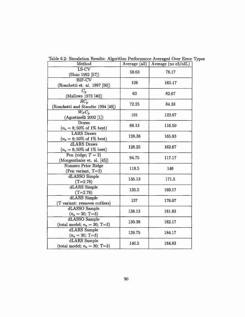
Table 6.2: Simulation Results: Algorithm Performance Averaged Over Error TypesMethod Average (all) Average (no e3/e3L)LS-CV LS-CV 58.63 78.17
(Shao 1992 [57])BIF-CV
126 165.17(Ronchetti et. al. 1997 [50])
CP 63 82.67(Mallows 1973 [40])
RCp 72.25 84.33(Ronchetti and Staudte 1994 [49])
WFCp 101 122.67(Agostinelli 2002 [1])
Draws 88.13 116.50(n = 8; 50% of 1% best)
LARS Draws128.38 165.83
(n8 = 8; 50% of 1% best)dLARS DrawsdLARS Draws 128.25 162.67
(n, = 8; 50% of 1% best)Pen (ridge; T = 2)
(Morgenthaler et. al. [45])Nonzero Prior Ridge 119.5 146(Pen variant, T=2)
dLASSO Simple 135.13 171.5(T=2.78)
dLARS Simple 135.5 169.17(T=2.78)
dLARS Simple(T variant: removes outliers)
dLASSO Sample 138.13 181.83(n8 = 30; T=3)
dLASSO Sample(total model; n, = 30; T=3)
dLARS Sample =3139.75 184.17(n, = 30; T=3)dLARS Sample
(total model; n, = 30; T=3)
90
Cp does give us approximately the same answer for e2, the "nice" outlier model, as
desired, with 120 out of 200 correct. Like LS-CV, Cp performs poorly on the e3 and
e4 error models.
Each of these standard model selection methods has a robust counterpart. For
LS-CV the robust counterpart is what we labeled BIF-CV [50] our the table. BIF-
CV is the current state-of-the-art in the published literature when it comes to robust
model selection. Other newer methods have been proposed but none of them have
been demonstrated to have as good of an accuracy rate as BIF-CV in simulations.
BIF-CV gets approximately 80% or more correct in each of the normal mixture model
errors (el, e2, and e4) for both the uniform and the leverage data models. BIF-CV
still has signficant trouble with the e3 error model, as we will see is the case for most
algorithms.
The robust counterparts of Cp are RCp [49] and WFCP [1]. RCp improves on the
robustness of Cp by doing much better in e3 and e4, but it performs worse in the el
and e2 error models. WFCP does even better by maintaining a similar percentage of
correctness in el and e2 to Cp and performing better than (in e4) or equivalent (in
e3) to RCp in the other error models. Still the absolute levels of correctness of WFCp
are lacking compared to BIF-CV.
The final two methods we consider from the literature are both from Morgenthaler
et. al. [45]. Draws at best does not seem to perform as well as BIF-CV either, but it
has a respectable showing. This is what lead us to believe that the Draws algorithm
is a good starting off point for a newer better algorithm. The Pen algorithm performs
comparably to BIF-CV in the uniform data model, but doesn't do as well when we
consider the possibility of leverage points. This is how we determined that the lever-
age case was one of the main weaknesses of the Pen algorithm. We attempted to
improve this aspect of the algorithm, while still maintaining the great performance
in the uniform data model.
Comparisons of Draws-type Methods
In Chapter 3, we describe the Draws Algorithm of Morgenthaler et. al. [45] and
91

we introduced a similar algorithm called LARS Draws, which attempts to improve
Draws by choosing models in a "smarter" way. In Chapter 5, we introduce a third
draws-types algorithm called dLARS Draws, which is similar to LARS Draws, except
it also includes the data dummy variables as described in Chapter 4.
Each of these algorithms relies upon the idea that fitting models from small sam-
ples of the data will lead to a higher breakdown procedure. They all also use the idea
that we can often get value out of combining a set of good variable selectors instead
of just relying on the one best answer. These algorithms differ both in the models
that are considered and in the coefficients that are fit for these models.
Tables 6.3 and 6.4 contain the results of a simulation study for comparing the
Draws-type methods. We use the Ronchetti et. al. data model as described in earlier
in this section. The numerical results represent the number of times we identify the
correct model from 200 different simulated data sets.
In order to have a more direct comparison of these algorithms, we tried to choose
the parameters the same for each algorithm. We took the same number of samples
(M = 500 or 2000) for each trial. The sample size was n, = 4 > p in order
to accommodate dLARS Draws. For Draws we chose p random models, for LARS
Draws we used the p models suggested by LARS, and for dLARS Draws we used the
ns models suggested by LARS. This will lead to dLARS Draws considering slightly
more models.
As described previously, the best models should be the ones with the lowest predic-
tion scores. In this simulation study we considered the models with prediction scores
in the bottom 1%, 5%, and 10%. In we fixed the number of samples () considered,
the final answers from using 1% were always best. The results were not dramatically
different however, so we do not report the results from the other percentages.
The prediction scores calculated as the MAD of the residuals associated with
predicting the out of sample data using the coefficients we estimated. For Draws
we use the OLS coefficients. For both LARS Draws and dLARS Draws, we consider
the LARS coefficients and what we called the "Combo" coefficients (recall these were
either the LARS or the OLS coefficients depending on which one gave us better
92

predictions).
Finaly a variable was selected if it appeared in more than a certain threshold num-
ber of times. We consider all three thresholds described under the heading "Variable
Selection Threshold" in Section 3.3.3. As in bagging we choose variables that appear
more than 50% of the time. We also consider the testing procedure described in
Section 3.3.3 with a = .05 (where we do not worry about the fact that we are consid-
ering p such tests) and a = .05/p (where we consider the Bonferroni approximation
for multiple testing).
Conclusions
We first note that we get better answers if we take more samples (2000 vs. 500). This
is expected because more samples should lead to us getting more clean samples. We
will explain other differences when we compare using 500 and 2000 samples, as a part
of our other conclusions.
Thern note that in all of the various parameters we considered, using LARS Draws
or dLAI:FS Draws is either strongly better than or in one instance approximately tied
with the Draws Algorithm results. The Draws Algorithm is approximately tied with
the LARS Draws with the LARS coefficients if we are considering the 50% threshold,
but in all other instances it is a much worse choice. This is an important conclusion
because it tells us that we should be better off using either of our new Draws-type
methods than the original Draws Algorithm.
Next, let us consider whether these results tell us anything about a preference
between using the dummy data variables or not using them. It is hard to declare a
"winner" here because there is no general trend indicating that one gives significantly
better answers across all eight categories. Perhaps a good interpretation of winner
is the method with the highest sum of correct answers across the eight categories.
93

Table 6.3: Simulation Results: Draws-type Algorithm Comparison - M = 500 andn, =8
Uniform LeverageMethod Parameters Uniform Leverageel e2 e3 e4 el e2 e3 e4
50% ofDraws 5% of 125 109 3 94 133 123 3 115
1% best
Draws 651 of 67 41 0 24 77 54 0 401% best
Draws 7 o 38 26 0 5 41 27 0 171% best
LARS Draws 50% ofLARSraws 170 of 108 116 9 106 149 159 21 144
LARS Draws 65.1% of 148 156 10 156 172 167 3 166LARS 1% best
LARS Draws 71.9% of 150 138 4 123 170 152 3 148LARS 1% best
LARS Draws 50% ofSCombo 50% tof 155 158 17 154 180 175 15 173
LARS Draws 65.1% of 157 141 5 128 173 160 3 165Combo 1% best
LARS Draws 71.9% of 136 127 4 107 160 138 3 145
dLARS 1%bDrawset o 157 1458 18 147 169 172 39 154
dLARS Draws 65.1% of 150 155 5 139 177 172 10 158LARCombo 1% best
dLARS Draws 71.9% of 131 133 3 106 163 158 4 143LARCombo 1% bestdLARS Draws 50% of
dLARS Draws 50% of 161 157 19 156 163 172 31 167LARS 1% best
dLARS Draws 65.1% of 152 155 7 142 173 173 9 160LARSombo 1% bestdLARS Draws 71.9% of 133 138 2 115 157 154 3 149Combo 1% best
Combo 1% best
94
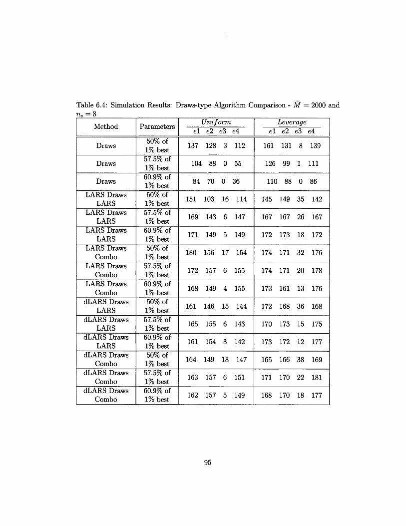
Table 6.4: Simulation Results: Draws-type Algorithm Comparison - M = 2000 andn, =8
Method Parameters Uniform Leverageel e2 e3 e4 el e2 e3 e4
50% ofDraws % best 137 128 3 112 161 131 8 139
1% best
Draws 57.5% of 104 88 0 55 126 99 1 1111% best
Draws 60.9% of 84 70 0 36 110 88 0 861% best
LARS Draws 50% ofLARS 1% best 151 103 16 114 145 149 35 142
LARS Draws 57.5% of 169 143 6 147 167 167 26 167LARS 1% best
LARS Draws 60.9% of 171 149 5 149 172 173 18 172LARS 1% best
LARS Draws 50% ofLARCombo 50 of 180 156 17 154 174 171 32 176Combo 1% best
LARS Draws 57.5% of 172 157 6 155 174 171 20 178Combo 1% best
LARS Draws 60.9% ofLARS Draws 60.9% of 168 149 4 155 173 161 13 176Combo 1% best
LARS 1%aws 50% of 161 146 15 144 172 168 36 168LARS 1% best
dLARS Draws 57.5% of 165 155 6 143 170 173 15 175LARS 1% best
dLARS Draws 60.9% ofLARS wst 161 154 3 142 173 172 12 177
LARS 1% best
SCombo 1%aws 505 of 164 149 18 147 165 166 38 169
dLARS Draws 57.5% of 163 157 6 151 171 170 22 181Combo 1% best
dLARS Draws 60.9% of 162 157 5 149 168 170 18 177Combo 1% best
95
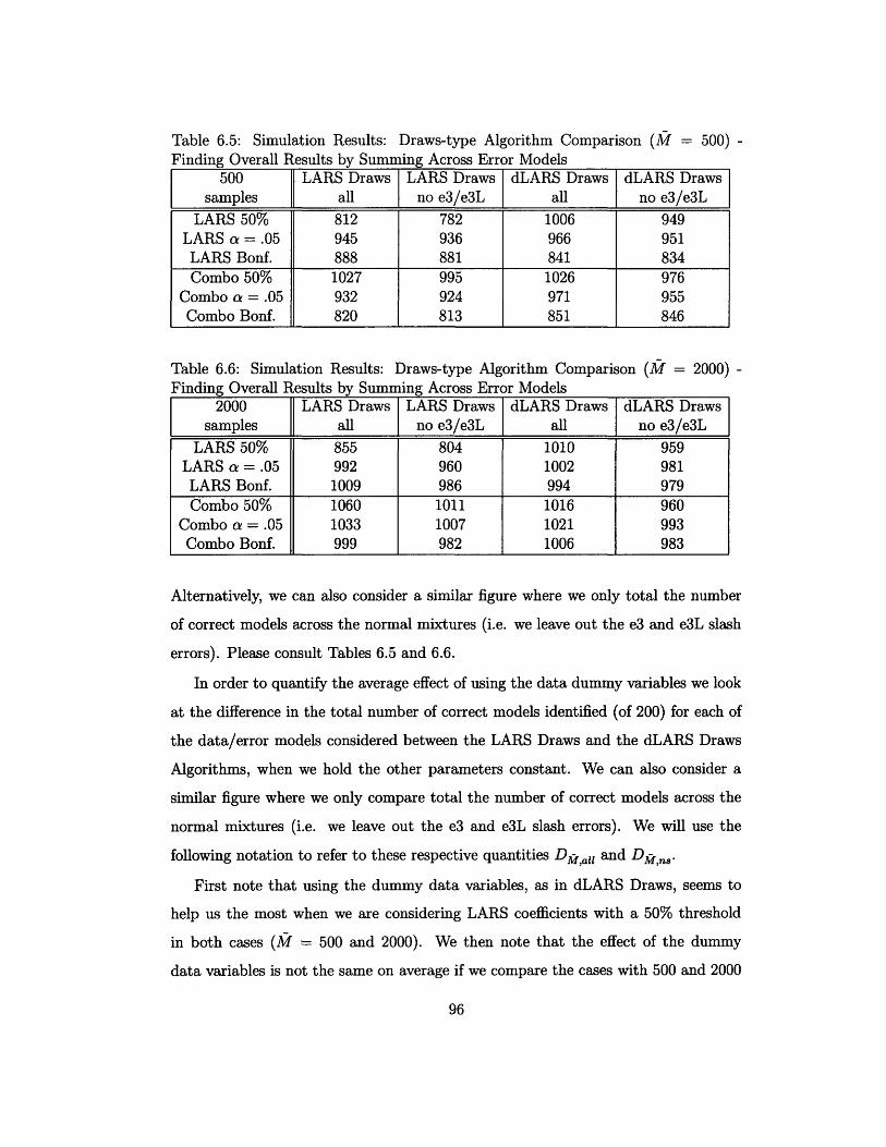
Table 6.5: Simulation Results: Draws-type Algorithm Comparison (M = 500) -Finding Overall Results by Summing Across Error Models
500 LARS Draws LARS Draws dLARS Draws dLARS Drawssamples all no e3/e3L all no e3/e3L
LARS 50% 812 782 1006 949LARS a = .05 945 936 966 951
LARS Bonf. 888 881 841 834Combo 50% 1027 995 1026 976
Combo a = .05 932 924 971 955Combo Bonf. 820 813 851 846
Table 6.6: Simulation Results: Draws-type Algorithm Comparison (M = 2000) -Finding Overall Results by Summing Across Error Models
2000 LARS Draws LARS Draws dLARS Draws dLARS Drawssamples all no e3/e3L all no e3/e3L
LARS 50% 855 804 1010 959LARS a= .05 992 960 1002 981LARS Bonf. 1009 986 994 979Combo 50% 1060 1011 1016 960
Combo a = .05 1033 1007 1021 993Combo Bonf. 999 982 1006 983
Alternatively, we can also consider a similar figure where we only total the number
of correct models across the normal mixtures (i.e. we leave out the e3 and e3L slash
errors). Please consult Tables 6.5 and 6.6.
In order to quantify the average effect of using the data dummy variables we look
at the difference in the total number of correct models identified (of 200) for each of
the data/error models considered between the LARS Draws and the dLARS Draws
Algorithms, when we hold the other parameters constant. We can also consider a
similar figure where we only compare total the number of correct models across the
normal mixtures (i.e. we leave out the e3 and e3L slash errors). We will use the
following notation to refer to these respective quantities Dk,a, and DM/,.
First note that using the dummy data variables, as in dLARS Draws, seems to
help us the most when we are considering LARS coefficients with a 50% threshold
in both cases (M = 500 and 2000). We then note that the effect of the dummy
data variables is not the same on average if we compare the cases with 500 and 2000
96
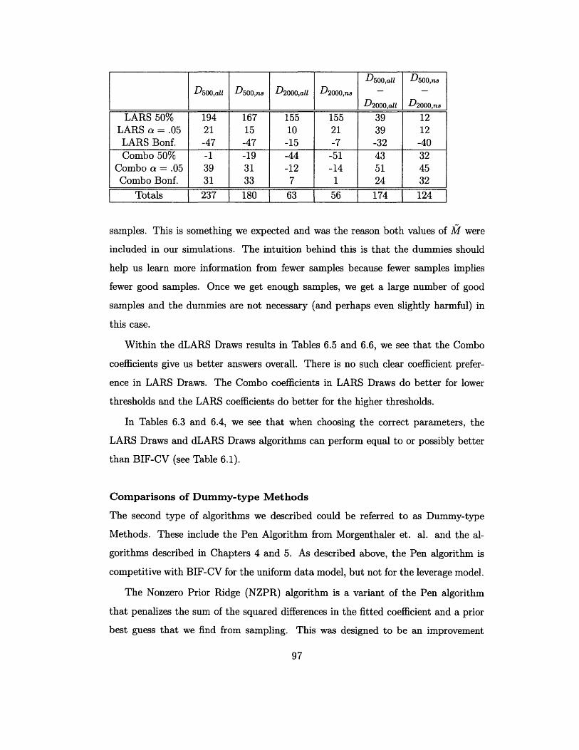
D500,all D5 00,ns
D500,all D 500 ,ns D2000,all D2000,ns - -D2000,all D20 00,ns
LARS 50% 194 167 155 155 39 12LARS a = .05 21 15 10 21 39 12LARS Bonf. -47 -47 -15 -7 -32 -40Combo 50% -1 -19 -44 -51 43 32
Combo a = .05 39 31 -12 -14 51 45Combo Bonf. 31 33 7 1 24 32
Totals 237 180 63 56 174 124
samples. This is something we expected and was the reason both values of M were
included in our simulations. The intuition behind this is that the dummies should
help us learn more information from fewer samples because fewer samples implies
fewer good samples. Once we get enough samples, we get a large number of good
samples and the dummies are not necessary (and perhaps even slightly harmful) in
this case.
Within the dLARS Draws results in Tables 6.5 and 6.6, we see that the Combo
coefficients give us better answers overall. There is no such clear coefficient prefer-
ence in LARS Draws. The Combo coefficients in LARS Draws do better for lower
thresholds and the LARS coefficients do better for the higher thresholds.
In Tables 6.3 and 6.4, we see that when choosing the correct parameters, the
LARS Draws and dLARS Draws algorithms can perform equal to or possibly better
than BIF-CV (see Table 6.1).
Comparisons of Dummy-type Methods
The second type of algorithms we described could be referred to as Dummy-type
Methods. These include the Pen Algorithm from Morgenthaler et. al. and the al-
gorithms described in Chapters 4 and 5. As described above, the Pen algorithm is
competitive with BIF-CV for the uniform data model, but not for the leverage model.
The Nonzero Prior Ridge (NZPR) algorithm is a variant of the Pen algorithm
that penalizes the sum of the squared differences in the fitted coefficient and a prior
best guess that we find from sampling. This was designed to be an improvement
97

that would help us with the leverage case and we see that it does. In the leverage
case, we see increases in the percentage correct of over 37% in all error models, which
lead to percentage point increases of 8.5 - 21.5%. This still doesn't improve our the
results enough to come close to how well BIF-CV performs. We do however also see
improvements in the uniform case too, so the NZPR algorithm ends up out-performing
BIF-CV in this case. So while we know that this method is still not good enough for
cases with leverage points, it might be a better choice for when we know there are no
leverage points.
The next set of algorithms are based on the LASSO penalty and the LARS algo-
rithm. Both the dLARS Simple and Sample Algorithms give great results. In fact in
general these algorithms seem to be the best of all of the ones we considered. Whether
we are using LASSO or Least Angle Regression for the original ordering does not seem
to matter, so for the sake of computational efficiency I recommend using Least Angle
Regression.
When we use the dLARS Simple variant that removes some suspected outliers, we
see that in most cases we do equal or better, except for the e3 error model. This leads
us to believe that this variant may be desired if we have reason to believe the error is
like a Normal mixture. If it has a very heavy-tailed distribution like slash or Cauchy,
we may be better off using the original version. The percentage we are getting correct
for e3 is so low that this difference may not have much practical importance however.
As hoped (and expected) we see improvements in the percentage correct in the
dLARS algorithm when we switch from the Simple to the Sample version. There
is also no difference in performance between selecting the variables independently of
each other or by choosing the model that is selected the most (total model version).
We did not detect a difference perhaps because of the design of the simulation. The-
oretically the total model version may be preferred, but this version has some storage
requirements that we may not be able to meet if p is very large.
Overall dLARS Sample is probably the robust model selection method that one
would recommend based on these simulations. A close second would be the dLARS
Simple, which would be desired if the Sample version becomes too computationally
98

burdensome.
6.1.2 An Alternative Correctness Measure
Khan et;. al. [34] have considered an alternative method of evaluating the correct-
ness of their algorithms under this framework. Given that LARS gives us a forward
ordering, they think that one way to test an algorithm is to see if at some step of the
robust version's ordering we have the correct model. We would just like to see all of
the important variables selected before the unimportant ones. We are less concerned
with the ordering among the important variables, but this is something we will also
consider.
Part of any of the penalty type methods is to choose the appropriate penalty
parameter. As we change the parameter we step through the different models. One
question we can ask is "with our method is there a correct choice for the penalty
parameter or cutoff in the case of LARS?" If we are getting an incorrect answer
based on this type of algorithm it could be because of two different things,
1. Our method is giving us a correct ordering at some step of the algorithm, but
we are not choosing the correct cutoff criterion.
2. For any choice of cutoff criterion, we could not get the correct model choice.
We are less concerned with getting the model incorrect because of the first reason
than the second. One reason is that perhaps the algorithm could be improved by
discovering a different method to determine the cutoff. Another is that it is not
recommended to consider just one model and in this case we know that the correct
model is among the choices of a reduced set of models. Specifically in the case of a
forward ordering type method we narrow the 2p models down to p models. Instead of
being burdened with a computationally infeasible all subsets problem that increases
exponentially, we only have to consider a number of models that increases linearly
with the number of original variables.
Most robust model selection algorithms do not lend themselves to this type of
evaluation because they do not rely on such an ordering. We can use this method
99
of evaluation to test our LARS Simple algorithm to determine if the addition of the
dummy variables for the data points actually is providing us with a robust ordering
of the variables. While this evaluation is not directly applicable to the LARS Sample
algorithms, one can easily see the indirect implications of the fact that the LARS
Simple algorithm is correctly ordering the variables.
In their simulations, they consider a modified version of the Ronchetti et. al. [50]
simulation framework. Khan et. al. [34] consider the same error distributions and
design matrices as in the Ronchetti et. al. with n = 60. In this new framework, the
only thing that changes is the settings of the coefficients. In this case only the first
three of the six coefficients are non-zero. They are set to 7, 5, and 3 respectively.
By changing the values of the coefficients, we can see whether the relative ordering
of the variables is correct amongst those with non-zero coefficients as well as whether
the variables with the non-zero coefficients are chosen before those with zero coeffi-
cients. Khan et. al. call these two performance measures the exact (E) and global
(G) respectively.
Once again we run this simulation on our dLARS Simple algorithm for 200 runs.
Note that our ordering is determined by the absolute size of the t-statistics from the
last step of the algorithm because the size of this t-statistic is how we determine final
inclusion. We are not assessing our algorithm by the ordering we get out of the step
where we perform the LARS algorithm on our dummy-modified data set.
In the following table, we record the values we received from our simulation, along
with the values in the Khan et. al. [34] paper from their simulations. They recorded
their values in terms of percentages, so we have converted our answers to percentages
to match the table in Khan et. al.
Both the Exact and the Global measurements of the performance of dLARS Simple
are practically equivalent to the measurements for the Khan et. al. Robust LARS
algorithm. This shows that our ordering used for selection in dLARS Simple is just
100

Table 6.7: Simulation Results: These are the results of a simulation comparing ourdLARS Simple algorithm to the algorithms from Khan et. al. [34] when consideringtheir alternative measure of correctness.
Uniform Leverageel e2 e3 e4 el e2 e3 e4
LARS-Exact 97 86 11 8 0 1 1 2
LARS- Global 100 89 26 24 0 2 5 7WP-Exact 96 97 58 78 92 85 46 59WP - Global 99 99 77 89 94 86 61 68WC-Exact 96 98 54 82 96 94 52 83WC - Global 99 99 76 92 98 96 71 92
dLARS Simple - Exact 95 95 61 83 96 95 65 85dLARS Simple - Global 100 100 80 88 100 99 85 91
as robust as the Khan et. al. Robust LARS ordering. Additionally the percentages in
all categories are fairly close to 100%. Even in the e3 cases we see Exact percentages
over 60% and Global percentages over 80%. This means that getting the correct
answers is just a matter of finding the right threshold for the T-statistic and that the
true answer is in our ordering most of the time.
This also means that if we decided to use dLARS Simple to narrow down the
possible models from 2p to p, then our true model would be contained in this narrowed
set most of the time. Further analysis of these narrowed models might allow us to
choose a threshold that leads us to better performances that we saw in Table 6.1.
Note, as described above our orderings were determined by the absolute size of the
t-statistics from the last step of the dLARS Simple algorithm. If we were to instead
test the ordering coming out the of LARS step within the algorithm, we would not
see the same kind of results (see Table B). The LARS step encourages us to choose
all of the correct variables and most/all of the correct outliers, but it does not give
them to us in the correct order necessarily. The t-statistic test was originally included
just to narrow down the number of selected variables from the upper bound. The
t-statistics have the added positive attribute that they give us a robust ordering of
the variables (as expected) when the original LARS step did not.
We presume that the fact that LARS, when performed on the dummy modified
data set, does not necessarily give us a robust ordering of the variables, is the main
101

reason we do not see a strong positive effect when we use the data dummies in dLARS
Draws. The dummies are still useful in helping us determine accurate coefficients and
can help to improve the original LARS ordering of variables, but they do not give us
near perfect orderings. This implies that they are not always helping us to start with
a better set of models than using LARS alone, as in LARS Draws.
6.2 Mortality Data
We also recognize that simulations alone do not allow us to correctly evaluate an
algorithm. We must also consider how the algorithm performs in a real-life situation.
We consider a data set on air pollution and mortality in 60 metropolitan areas in the
United States. This data set is publicly available in the Data and Story Library of
Statlib. We will refer to this data set as the mortality data.
The outcome variable is age-adjusted mortality. The explanatory data include
variables measuring demographic characteristics of the cities, variables measuring cli-
mate characteristics, and variables recording the pollution potential of three different
air pollutants.
There are 14 potential predictors:
1. Mean January temperature (degrees Farenheit)
2. JulyTemp: Mean July temperature (degrees Farenheit)
3. RelHum: Relative Humidity
4. Rain: Annual rainfall (inches)
5. Education: Median education
6. PopDensity: Population density
7. %NonWhite: Percentage of non whites
8. %WC: Percentage of white collar workers
102

Table 6.8: Models Selected from Various Algorithms
9. pop: Population
10. pop/house: Population per household
11. income: Median income
12. logHCPot: natural log of HC pollution potential
13. logNOxPot: natural log of Nitrous Oxide pollution potential
14. logSO2Pot: natural log of Sulfur Dioxide pollution potential
(Note: In the data set on Statlib there are actually 15 predictors, but one variable
is included twice. Also it is recommended that we consider the log of the pollution
variables due to the skewness of the original set. Also, given that row 21 contains 2
missing values, we will disregard this data point.)
There is no set of important variables or set of outliers that is well-recognized
by the statistics community as the true model. We will attempt to determine this
through our various analyses.
6.2.1 Selected Models
Each of the different model selection algorithms has a different way of selecting the
model and thus each might lead to a different choice. The following are the top choices
for the various algorithms we considered. These include both robust and non-robust
algorithms.
103
Algorithm Variables SelectedBest Subsets - BIC 1,4,5,7,13
Best Subsets - AIC/Cp 1,4,6,7,8,13Draws 7,4,14,6
LARS Draws 7,4,6,14,5dLARS Draws 7,4,6,14,5,3,9
Nonzero Prior Pen 6,14,7,4,9,5dLARS Simple 7,4,14dLARS Sample 7,4,6,14,1,8
All of the models have 4 (Rain) and 7 (Percentage of Nonwhite people). This
indicates that these variables have a strong enough signal to be detected even in
the presence of outliers. Most also have 6 (Population Density), a pollution poten-
tial variable like 13 (NOx) or more likely 14 (S02), and one of 5 (Education) or 8
(Percentage of White Collar Workers).
One main difference we see between the robust and non-robust algorithm selections
is that the robust ones choose 14 where the non-robust ones choose 13. Both of these
are pollution variables, but the robust algorithms seem to think that given the other
variables in consideration, S02 has a stronger relationship to mortality than NOx.
Additionally the non-robust algorithms seem to put more of an emphasis on selecting
variable 1, Mean January Temperature.
6.2.2 Which model is best?
These models are clearly different, but which models are better than the others? In
an ideal setting we might have enough data that we could split it up into a training
set, a validation set, and a test set. Then we could use the training set to find the
models and fit coefficients for each model. Then we could use the test set to test
which models give us the best predictions. Unfortunately with as many variables as
we were considering in the beginning, it was not possible to set aside enough data
for a test set. Instead, we will look at three different sets of statistics to compare the
models.
First, we use a robust high-breakdown algorithm (LTS) to determine appropriate
coefficients for each of the selected variables. From here we can use robust estimates
like the LTS scale estimate, MAD of the LTS residuals, and robust R 2 to compare
how well each of these models fits the data. All of these were calculated using the
Robust LTS Regression procedure in S-Plus 7.0. The number of squared residuals
to trim was chosen to match our assumption in the selection phase of at most 25%
contamination. There is no reason to doubt this assumption for this data set.
As we can see from the above table, our robust algorithms choices are in general
better in terms of the various statistics we considered. Our worst performing method
104
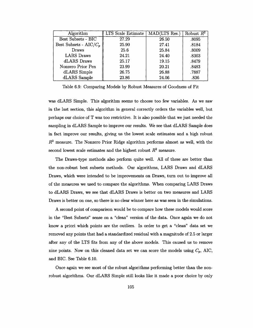
Algorithm LTS Scale Estimate MAD(LTS Res.) Robust R2
Best Subsets - BIC 27.29 26.50 .8095Best Subsets- AIC/Cp 25.90 27.41 .8184
Draws 25.6 25.84 .8009LARS Draws 24.21 24.40 .8303
dLARS Draws 25.17 19.15 .8479Nonzero Prior Pen 23.99 20.21 .8483
dLARS Simple 26.75 26.88 .7887dLARS Sample 23.86 24.06 .836
Table 6.9: Comparing Models by Robust Measures of Goodness of Fit
was dLARS Simple. This algorithm seems to choose too few variables. As we saw
in the last section, this algorithm in general correctly orders the variables well, but
perhaps our choice of T was too restrictive. It is also possible that we just needed the
sampling in dLARS Sample to improve our results. We see that dLARS Sample does
in fact improve our results, giving us the lowest scale estimates and a high robust
R2 measure. The Nonzero Prior Ridge algorithm performs almost as well, with the
second lowest scale estimates and the highest robust R2 measure.
The Draws-type methods also perform quite well. All of these are better than
the non-robust best subsets methods. Our algorithms, LARS Draws and dLARS
Draws, which were intended to be improvements on Draws, turn out to improve all
of the measures we used to compare the algorithms. When comparing LARS Draws
to dLARS Draws, we see that dLARS Draws is better on two measures and LARS
Draws is better on one, so there is no clear winner here as was seen in the simulations.
A second point of comparison would be to compare how these models would score
in the "Best Subsets" sense on a "clean" version of the data. Once again we do not
know a priori which points are the outliers. In order to get a "clean" data set we
removed any points that had a standardized residual with a magnitude of 2.5 or larger
after any of the LTS fits from any of the above models. This caused us to remove
nine points. Now on this cleaned data set we can score the models using Cp, AIC,
and BIC. See Table 6.10.
Once again we see most of the robust algorithms performing better than the non-
robust algorithms. Our dLARS Simple still looks like it made a poor choice by only
105
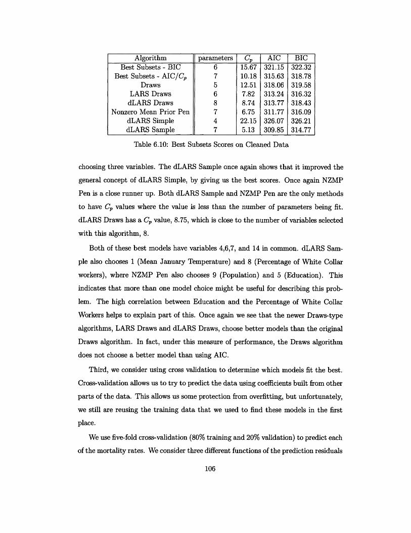
Algorithm parameters Cp AIC BICBest Subsets - BIC 6 15.67 321.15 322.32
Best Subsets - AIC/Cp 7 10.18 315.63 318.78Draws 5 12.51 318.06 319.58
LARS Draws 6 7.82 313.24 316.32dLARS Draws 8 8.74 313.77 318.43
Nonzero Mean Prior Pen 7 6.75 311.77 316.09dLARS Simple 4 22.15 326.07 326.21dLARS Sample 7 5.13 309.85 314.77
Table 6.10: Best Subsets Scores on Cleaned Data
choosing three variables. The dLARS Sample once again shows that it improved the
general concept of dLARS Simple, by giving us the best scores. Once again NZMP
Pen is a close runner up. Both dLARS Sample and NZMP Pen are the only methods
to have Cp values where the value is less than the number of parameters being fit.
dLARS Draws has a Cp value, 8.75, which is close to the number of variables selected
with this algorithm, 8.
Both of these best models have variables 4,6,7, and 14 in common. dLARS Sam-
ple also chooses 1 (Mean January Temperature) and 8 (Percentage of White Collar
workers), where NZMP Pen also chooses 9 (Population) and 5 (Education). This
indicates that more than one model choice might be useful for describing this prob-
lem. The high correlation between Education and the Percentage of White Collar
Workers helps to explain part of this. Once again we see that the newer Draws-type
algorithms, LARS Draws and dLARS Draws, choose better models than the original
Draws algorithm. In fact, under this measure of performance, the Draws algorithm
does not choose a better model than using AIC.
Third, we consider using cross validation to determine which models fit the best.
Cross-validation allows us to try to predict the data using coefficients built from other
parts of the data. This allows us some protection from overfitting, but unfortunately,
we still are reusing the training data that we used to find these models in the first
place.
We use five-fold cross-validation (80% training and 20% validation) to predict each
of the mortality rates. We consider three different functions of the prediction residuals
106
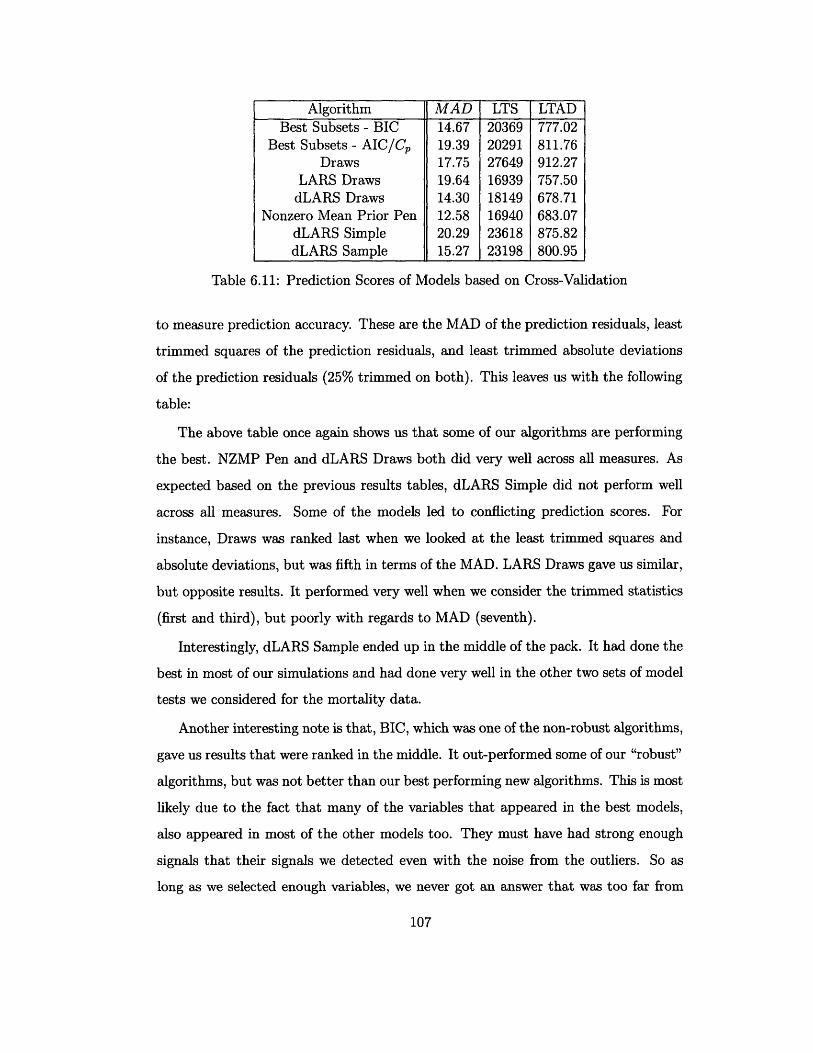
Algorithm MAD LTS LTADBest Subsets - BIC 14.67 20369 777.02
Best Subsets - AIC/Cp 19.39 20291 811.76Draws 17.75 27649 912.27
LARS Draws 19.64 16939 757.50dLARS Draws 14.30 18149 678.71
Nonzero Mean Prior Pen 12.58 16940 683.07dLARS Simple 20.29 23618 875.82dLARS Sample 15.27 23198 800.95
Table 6.11: Prediction Scores of Models based on Cross-Validation
to measure prediction accuracy. These are the MAD of the prediction residuals, least
trimmed squares of the prediction residuals, and least trimmed absolute deviations
of the prediction residuals (25% trimmed on both). This leaves us with the following
table:
The above table once again shows us that some of our algorithms are performing
the best. NZMP Pen and dLARS Draws both did very well across all measures. As
expected based on the previous results tables, dLARS Simple did not perform well
across all measures. Some of the models led to conflicting prediction scores. For
instance, Draws was ranked last when we looked at the least trimmed squares and
absolute deviations, but was fifth in terms of the MAD. LARS Draws gave us similar,
but opposite results. It performed very well when we consider the trimmed statistics
(first and third), but poorly with regards to MAD (seventh).
Interestingly, dLARS Sample ended up in the middle of the pack. It had done the
best in most of our simulations and had done very well in the other two sets of model
tests we considered for the mortality data.
Another interesting note is that, BIC, which was one of the non-robust algorithms,
gave us results that were ranked in the middle. It out-performed some of our "robust"
algorithms, but was not better than our best performing new algorithms. This is most
likely due to the fact that many of the variables that appeared in the best models,
also appeared in most of the other models too. They must have had strong enough
signals that their signals we detected even with the noise from the outliers. So as
long as we selected enough variables, we never got an answer that was too far from
107

correct.
6.2.3 Simulations vs. Real Data
Simulations are useful to test algorithms because we know the "correct answer." As
we saw in the real data case, it is hard to compare the algorithms if we don't know
the correct answer. We looked at many different measures of goodness of fit and
sometimes got contradictory results. Real data examples are still important though
because real data will never have an error distribution that exactly matches the ones
we test the algorithm against. For instance, in the case of the mortality data, the
Nonzero Mean Prior Pen Algorithm from Chapter 5.2 seemed to overall perform the
best, but it was not the top rated algorithm with regards to the simulations.
NZMP Pen was one of the best with regards to the slash type error. Similarly
LARS Draws and dLARS Draws performed comparatively well on the slash error
and also gave us similar models to the NZMP Pen algorithm for the mortality data.
Perhaps the mortality data had outliers that made the data have fatter tails than
in the Normal mixture models we considered in the simulations, so it needed an
algorithm that performs better on this type of data.
Given there is no need to only consider one model when studying a data set,
we recommend considering the models suggested by all of the top algorithms. This
should both allow to narrow down the models to a manageable set and not force us
to choose between algorithms with differing strengths.
108

Chapter 7
Diagnostic Traces and Forward
Search
This chapter focuses on a diagnostic methods to discover outliers or groups of outliers
in our data set, as well as to elucidate the effects of each observation on various
inferences. The outcome of the diagnostics is a set of different plots that are very
similar to the types of plots from Atkinson and Riani's Forward Search [5], but the
process of creating the requisite statistics and plots is very different.
In this chapter, we assume that we know the model for the data. By "know the
model", we mean that we know which variables and functions of variables that will
make up the linear regression equation, but we do not necessarily know the coefficients
on these terms. The diagnostics that we introduce could be adjusted to account for
model uncertainty, but this is not the main focus of this chapter.
7.1 Outlier Detection
In Chapter 2, we discussed how a large part of the robustness literature is focussed on
outlier detection. In fact the literature on this problem is fairly extensive, especially
in contrast to the robust model selection literature. Outlier detection would be simple
if the true error variance and true coefficients were known for the model. Then we
could easily identify the outliers as the points which grossly deviate from the specified
109

model, i.e. points with excessively large residuals relative to the error variance. The
whole challenge of regression is that, even given the right choice of variables, the
coefficients and error variance are unknown and we need the data to tell us what are
good estimates for these values.
When we use outliers to help us to fit estimates of the parameters, the values can
end up badly biased. This can cause two undesirable phenomena called outlier mask-
ing and swamping. Masking occurs when a set of outliers goes undetected because of
the presence of another set of outliers. Swamping occurs with "good" observations
are misidentified as outliers because of the presence of a set of outliers. [7],[18], [21],
[22].
Given this, many methods for outlier detection aim to separate the data into two
sets: the "clean" set and the set of possible outliers [21],[22]. There are two possible
interpretations of what the clean set is. One is that the clean points are all of the
points that are not vertical outliers or leverage (both good and bad) outliers. These
points are what one might call the regular points, given none look out of the ordinary
in any way. The other interpretation is that the clean points are all of the points that
are not vertical outliers. This second case allows good leverage points to be in the
clean set.
There are advantages and disadvantages to both interpretations. Leverage points
typically have a strong influence on the regression line. Excluding all leverage points
protects us from bad leverage points that we might have misidentified as good leverage
points. We need to be sure that they are truly good leverage points to want to include
them in our analysis because of the risk they pose in confusing our results. Good
leverage points are called "good" for a reason though. Sometimes we add leverage
points to the explanatory data that we collect because they can help is to better
understand our regression function over a wide range of x's and they lead us to
smaller standard errors on our coefficient estimates. Excluding these good leverage
points means that we lose valuable information about our data and the regression
function that we are trying to estimate.
Given the advantages and disadvantages of including or excluding the good lever-
110

age points in the "clean" set, we recommend considering both types of "clean" sets.
We can then compare the coefficients to see if adding the good leverage points leads
us to very different results or if the good leverage points look bad given the model
developed from the regular points alone.
Assuming we can accurately identify a clean set, it can safely be used for parameter
estimation. Once outliers are identified, we can also attempt to discover why they
are different from the bulk of the data.
Some of the earliest ideas to address outlier masking are the leave-one-out deletion
techniques [8]. In these methods we remove one of the data points and calculate the
variance statistics of interest without this point. By not using this one point in the
calculations, we are not allowing this point to influence our estimates. This allows us
to get a more objective view on whether this point agrees with the rest of the data.
We can then do this for each of the n data points. These types of methods can work
well if the number of outliers is small and they are spread out, however these methods
completely fall apart when we get groups of outliers.
For instance, assume we have a pair of similar outliers. When we use a leave-one-
out deletion technique, we only remove one of the two points before the estimation
phase. The second point is still free to influence the estimates. It is possible that this
other point could influence the estimates enough that we can no longer determine
that the point we removed is abnormal.
Given this last example, an obvious extension of the leave-one-out technique is to
then remove pairs of outliers, but once again all we would need is a group of three
outliers to have masking problems again. It is obvious that it is not computationally
possible to extend this technique to any size group of outliers for even a moderate
size data set.
So the goal of any effective robust diagnostic like ours would be to find the outliers
even in the presence of masking in a computationally efficient manner. One idea that
meets these criteria is Atkinson and Riani's Forward Search [5].
111

7.2 Forward Search
The idea behind Atkinson and Riani's forward search is that instead of using a "back-
ward" approach, that is starting from the full data set and removing outliers one or
more at a time, we should use a "forward" approach and start with very small, but
clean data set and grow the non-outlier set in size by one each step, creating a larger
"clean" data set. We continue to add back points until the whole data set set has been
included back in. Then we compare the different data sets on a number of different
diagnostic statistics to discover which ones are clean and which ones have outliers.
The beginning set is found by using a robust high-breakdown method to find the
"cleanest" elemental set. In this case the high-breakdown method should protect
us from both vertical and leverage outliers. Given the regression solution that the
high-breakdown method suggests, we choose the points closest to the regression line.
This "cleanest" elemental set can include leverage points that the high-breakdown
method suggests are good. We increase the size of the set by one data point each
step, but we are not necessarily always adding one point to the set. For example, it is
possible to add two and remove one. This may seem more like a stepwise method, but
it is viewed as forward in the sense that the cardinality of the "clean" set is always
growing by one each step.
This ordering of the data takes us from a very small set with a robust fit to the full
data set and an ordinary least squares fit. If the models fit from the successive data
sets agree, we should see very little change in statistics such as coefficient values,
squared residuals, etc. over the course of the search. Although the addition of a
new point like an outlier to the "clean" set might drastically change some of these
statistics. The plots made will give us an idea of which statistics are affected by the
outliers and how these statistics are affected.
7.2.1 The Forward Search Algorithm
Initial Subset
Assuming that the model contains p variables as before, or q = p+ 1 total parameters
112

including the intercept, we need to start our algorithm with q points in order to fit
the q coefficients. If n is moderate and q << n then we can test all (n) possible sets
of q points. Otherwise, we test a large number of samples of size q from the data.
Despite the fact that we will neither be guaranteed to have a unique or completely
optimal solution, sampling methods like this are well accepted in robust statistics [5].
Let I be a set q of row indices {il,... , iq}. Let eij, be the least squares residual
for observation i given the observations in set I. We choose the initial subset as the
observations with the indices in the set I* which satisfies,
I* = argmin [e[Ln+q+lj],I] (7.1)
where [i] refers to the ith order statistic of the vector. Which gives us the initial
subset of,
Np+ = {xili E I*} (7.2)
According to the authors, the search is even able to recover from a poor starting
subset as long as there are no masked outliers included in the initial subset. They
also remark that instead of a Least Median of Squares criterion, we could have tried a
Least Trimmed Squares criterion for this step, but they found little difference between
these two procedures for the data sets they considered.
Adding Observations
At the beginning of an iteration, we start with a subset with the indices Im that is
of size mn > q. We fit a least squares model on this subset and calculate the squared
residuals, e2I( )i=l n We order the squared residuals and find the points with the
m + 1 lowest squared residuals to create the set of indices I(m+1). Typically the new
set contains the old set, but this is not always the case. When we add an outlier, the
estimates sometimes can change enough that a new set of points are closer to the fit.
(Note: Often we just end up swapping a few points and there are ways to calculate
the new coefficient estimates quickly based on the old estimates. We will not address
113
this here. A useful reference for the details and a list of other appropriate references
is [5].)
We repeat this step until all of the points have been added back to the set. We
save the least squares coefficient estimates for all of the sets in,
= (q) ***X3n)) (73)
We save the residuals in,
eFS = (e(q) e()) (7.4)
We also save the residual mean square estimates for each of the least squares fits,
SI(m), for the mth subset. These estimates are calculated only for the points that are
in the active data set. We see that, even when our full data set is clean, for m < n,
SI(m) < SI(n) = Sfull' (7.5)
Plotting
We take all of the values calculated in the previous step and we create a number of
different plots to study the behavior of the data as we add in new points.
Monitoring Coefficient Estimates - We can monitor coefficients in two ways, by
their absolute size and by their t-statistics (assuming they were calculated in the last
step.) Possible plots include m vs. 3t(m) and m vs. t(/(m)) (see Figure 7-1).
Monitoring Residuals - Large values of residuals are an indicator of possible out-
liers. We standardize all of the residuals by the final root mean square estimate, sfull
because the other estimates of ar are too dependent on the size of the data set for
that step [5]. We can look at the plots of m vs. (m))/sfull (see Figure 7-2) and m
vs. (e(m))2/sfull (see Figure 7-3).
Error variance and R 2 - Outliers artificially inflate our estimates of the error
variance. We can look at a plot of m vs. I(m) (see Figure 7-4) to see where there
are sharp increases in our estimates of the standard deviation, which indicate the
114
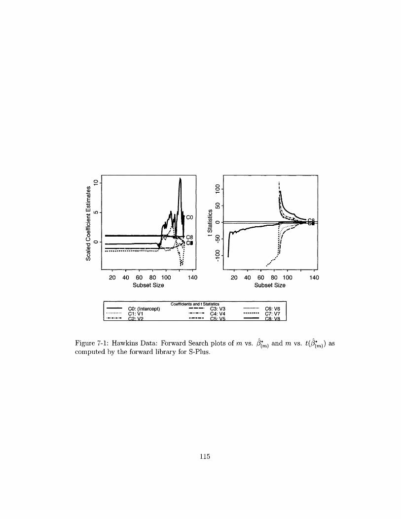
0U)a)
EU,
LOCa)
n
.5a)00-0 0a)CZU
U)
20 40 60 80 100Subset Size
00
0
U)
0.O
L)
00
140 20 40 60 80 100Subset Size
140
Coefficients and t StatisticsCO: (Intercept) . C3: V3 I....... C6: V6I " C1: V1 "..," C4:V4 ........ C7:V7
''''''- C2. VP C:V V- CR- VR
Figure 7-1: Hawkins Data: Forward Search plots of m vs. 3(m) and m vs. t(3(m)) ascomputed by the forward library for S-Plus.
115
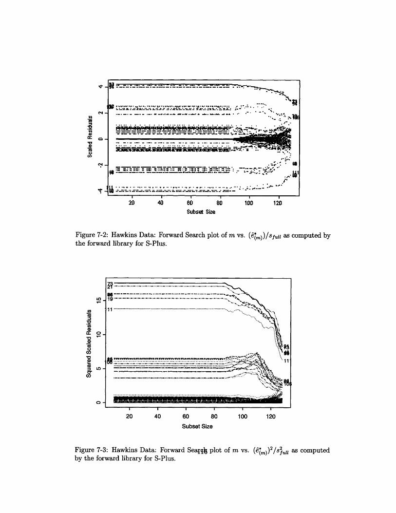
,,, =~ , ~~, ~ ,, - -,:.-X -- Z--- -,Z .' ....
*... .s .. .. . . ... ,i, .. .I .. . ..'. ................ .·jj... .- .
." .. ... ....... .... .. ...... .. .. __..r=."_"___ _' _ _ __ _ _ -""~ . . : _ - .. 'J *s.-s ;!CW~~ ~&"lt mlt _ ~-~,'. -- ..
,.='.'' * U
....... *_-_,.' --' 'r. ?-".,*._,.'--=m = ..'- r._- '- - - -.
;'· · ·~~~~ ~~· . .· ·i s v X X . , - -- ............ --i ,· ,fu ,. *,_.-
~~~~~~~~-
-- -= --c = = -_ =__- ' '-· , ·' re·~In~· 'I'C· I· I ~ I'
20 40 60 80 10 220 40 60 B0 lO0 l20
Subset Size
Figure 7-2: Hawkins Data: Forward Search plot of m vs. ())/sfu as computed bythe forward library for S-Plus.
I I I I
20 40 60 80 100 120
Subset Size
Figure 7-3: Hawkins Data: Forward Sea{¶ plot of m vs. (2)) /s2by the forward library for S-Plus.
as computed
.U-
N
,n
P'=
a'm
Ca
C
N.
L .qf.
.5
cr
O
0nC,,
0o
LO -
11 . ,,,, , , ,,, ,",,>- :..,.N.. ,¥, \'""... '
....... . ~'Sii...-'?':-'~:4 ~ ,\\1
.. .,, ,,,,....... ,,.,,.,,,,,, .......................... . .................................... .. 1as T~rrrr7TrY: z. - _s'.t. ·
*4,
0 -
96 --------------------------------- "I-,,
1
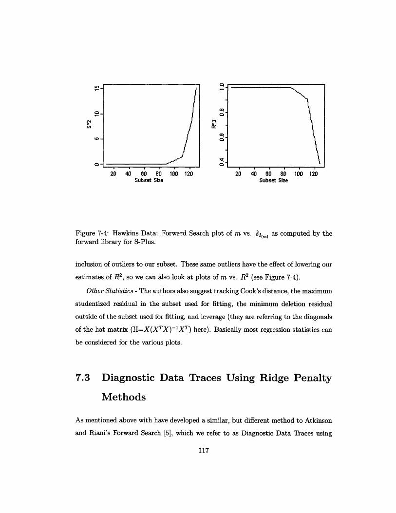
C
,C -
o
00
C4
c
Ca
-I J
20 40 60 80 100 120 20 40 60 80 100 120Subset Size Subset Size
Figure 7-4: Hawkins Data: Forward Search plot of m vs. si(~) as computed by theforward library for S-Plus.
inclusion of outliers to our subset. These same outliers have the effect of lowering our
estimates of R 2, so we can also look at plots of m vs. R2 (see Figure 7-4).
Other Statistics - The authors also suggest tracking Cook's distance, the maximum
studentized residual in the subset used for fitting, the minimum deletion residual
outside of the subset used for fitting, and leverage (they are referring to the diagonals
of the hat matrix (H=X(XTX)-IXT) here). Basically most regression statistics can
be considered for the various plots.
7.3 Diagnostic Data Traces Using Ridge Penalty
Methods
As mentioned above with have developed a similar, but different method to Atkinson
and Riani's Forward Search [5], which we refer to as Diagnostic Data Traces using
117
a~~~~~~~~~~~~~~~· _ * -MM
I I
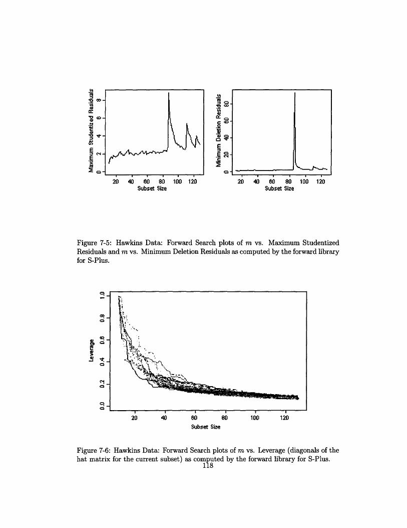
IA
',.v
Xc'.4
c ,
20 4 60 80 Subset Size
m
a
. - .C 0
E
0-c_
C3
100 120 20 40 60 80Subset Size
Figure 7-5: Hawkins Data: Forward Search plots of m vs. Maximum StudentizedResiduals and m vs. Minimum Deletion Residuals as computed by the forward libraryfor S-Plus.
-
1!
0R
0
N cq
-
I I I I I I
20 40 60 80 100 120
Subset Size
Figure 7-6: Hawkins Data: Forward Search plots of m vs. Leverage (diagonals of thehat matrix for the current subset) as computed by the forward library for S-Plus.
118
100 120
"~ _
_ r
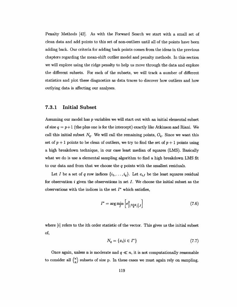
Penalty Methods [42]. As with the Forward Search we start with a small set of
clean data and add points to this set of non-outliers until all of the points have been
adding back. Our criteria for adding back points comes from the ideas in the previous
chapters regarding the mean-shift outlier model and penalty methods. In this section
we will explore using the ridge penalty to help us move through the data and explore
the different subsets. For each of the subsets, we will track a number of different
statistics and plot these diagnostics as data traces to discover how outliers and how
outlying data is affecting our analyses.
7.3.1 Initial Subset
Assuming our model has p variables we will start out with an initial elemental subset
of size q = p+ 1 (the plus one is for the intercept) exactly like Atkinson and Riani. We
call this initial subset Nq. We will call the remaining points, Oq. Since we want this
set of p + 1 points to be clean of outliers, we try to find the set of p + 1 points using
a high breakdown technique, in our case least median of squares (LMS). Basically
what we do is use a elemental sampling algorithm to find a high breakdown LMS fit
to our data and from that we choose the q points with the smallest residuals.
Let I be a set of q row indices (il,..., iq). Let ei,j be the least squares residual
for observation i given the observations in set I. We choose the initial subset as the
observations with the indices in the set I* which satisfies,
I* = arg min [e[Ln+ ] (7.6)
where [i] refers to the ith order statistic of the vector. This gives us the initial subset
of,
Nq = ({Xli E I*) (7.7)
Once again, unless n is moderate and q < n, it is not computationally reasonable
to consider all (q) subsets of size p. In these cases we must again rely on sampling.
119

We could consider other methods besides Atkinson and Riani's choice of LMS. Other
options include least trimmed squares (LTS) and bounded-influence methods.
7.3.2 Adding Back Data Points
The next step is to conduct a forward-type search through the data points to see
which points should belong in the "cleanest" subsets of size q + 1, q + 2, ... , n, which
we will call Nq+, Nq+2, ... , Nn respectively. In Chapters 4 and 5, we used penalty
methods to select which variables were important and most importantly which data
points were outliers.
When we start with a very small penalty parameter, we will fit many significant
coefficients on the data variables because we have made it easier for these variables
to have larger coefficients. This indicates that there are very few non-outliers. As we
increase the penalty, it becomes harder for the data dummy variables to be fit with
significant coefficients. Slowly more data points are added to the set of non-outliers.
We use this idea as a way to create our own version of the forward search.
Since we have reason to believe that our initial set Nq is a clean data set repre-
sentative of the bulk of the data, we do not need to create any dummy variables to
represent these data points. (Note: One may want to retest this supposition over the
course of the algorithm, we will address this in a later section.) Also for this algo-
rithm, we are only going to apply the penalty to the data variables that we do create,
corresponding to the points in the set Oq. This is because we are only interested in
varying the selection of the outliers and non-outliers. We are assuming that we have
discovered the true model, so we do not penalize the original explanatory variables.
One could consider a variant of this algorithm where we do not know the model and
in this case adding penalties on the original variables might be useful.
We proceed similarly to our algorithms in Chapters 4 and 5, by augmenting the
data set with dummy data variables, except for the fact that we do not add data
variables for the q points in the initial subset. Suppose that we have reordered the
points in the data set so that the points in the initial subset now have the indices
1, ... , q Then our new matrix of explanatory variables is the n x n matrix
120

1 X11 X 12 ... X1p 0 0 ... 0
1 2 1 X22 ... 0 0 ... 0
Z= (XA) 1 Xql xq2 ... Xqp 0 0 ... 0(7.8)Z=(XA)= (7.8)
1 X(q+l)l X(q+l)2 ... X(q+l)p 1 0 ... 0
1 X(q+2)1 X(q+2)2 ... X(q+2)p 0 1 ... 0
1 Xnl Xn2 ... Xnp 0 0 ... 1
where A consists of the n - q columns of the n x n identity matrix where there is a
single one in the row corresponding to the points in Oq.
Also note above that we have included the columns of ones for the intercept term.
We do not need to center the data because we are no longer penalizing the true
variables. Thus, our choice of origin is no longer an issue with regards to using a
penalty method as it was before. Nor do we have to scale the original variables any
longer. Scaling was required before because when including a penalty on a variable,
the rate of shrinkage is a function of the variance of the variable.
As described above, we are now going to use penalty methods to help us vary
the number of significant dummy variables and thus vary the number of data points
included in the clean subset. Once again the first penalty function we considered
was the ridge penalty, except now, as described above, we do not include all of the
coefficients in the function.n-1
J(z)= E i=q
equivalently,n-I
AJ(z) = E Aii=O
where Ai = A for i = q,..., n - 1 and Ai = 0 otherwise.
(7.9)
(7.10)
121
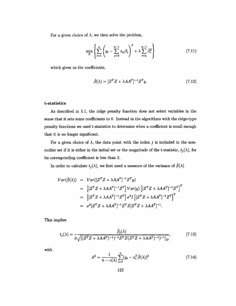
For a given choice of A, we then solve the problem,
min Yi - E zijj + A (7.11)-i=1 j:0 i=q
which gives us the coefficients,
/(A) = [ZTZ + AAAT]-ZTy. (7.12)
t-statistics
As described in 5.1, the ridge penalty function does not select variables in the
sense that it sets some coefficients to 0. Instead in the algorithms with the ridge-type
penalty functions we used t-statistics to determine when a coefficient is small enough
that it is no longer significant.
For a given choice of A, the data point with the index j is included in the non-
outlier set if it is either in the initial set or the magnitude of the t-statistic, tj(A), for
its corresponding coefficient is less than 2.
In order to calculate tj(A), we first need a measure of the variance of (A)
Var(/3(A)) = Var([ZT Z + AAAT]-ZTy)
= [[ZTZ + AAAT]1ZT] Var(y) [[ZTZ + AAAT]lZT]T
= [[ZTZ + AAAT]1LZT] U21 [[ZTZ + AATIV.ZT]T
= a2 [ZTZ + AAAT]-lZTZ[ZTZ + AAAT]-1.
This implies
j() /[(ZTZ + AAAT)-)-lZTZ(ZTZ + AAT)-i)-i]jj (7.13)
with1 n
~a. 2 h>)s(Yi _ XT (kA) (7.14)
122122

and
c(A) = trace (Z(ZTZ + AAT)ZTy). (7.15)
where the function c(A) above is a common measure of complexity or equivalent
degrees of freedom [24].
The above calculation of the t-statistics comes from the ridge regression view of
the problem. There is one challenge to using this calculation though. As k - 0oo,
both the coefficient estimates and the standard error estimates are being driven to
zero, as desired. However the standard error estimate is going to zero faster than the
coefficient estimate. This means that after a certain point, all of the data variables
will measure as significant variables, even if the size of their coefficient has no practical
significance.
This turning point can occur before we have added back all of the points to the
non-outlier model. This will often occur when we have some very large outliers. This
will limit our ability to get a full trace of each of the statistics. We also must limit
our plots to the models determined before this turning point otherwise the plots will
start backtracking.
An Alternate View Using Mixed Estimation
There is an alternate view of problem, however, that will give us a different way of
calculating the standard errors. By viewing the problem as a mixed estimation, we
will no longer have the problem of the subset size shrinking back to p. Mixed esti-
mation was introduced by Theil and Goldeberger [60]. This technique uses the prior
information by augmenting the data directly instead of using a prior distribution, as
in the Bayesian model.
In mixed estimation, we assume that we can write a set of restrictions on the
coefficients, 3, of the form
a = D/ + 6 (7.16)
where E(6) = 0, Var(6) = V, D is an r x p matrix of known constants, and a is an
r x 1 vector of random variables. We can then treat these equations as new data and
123
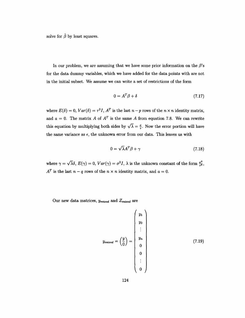
solve for p by least squares.
In our problem, we are assuming that we have some prior information on the p3's
for the data dummy variables, which we have added for the data points with are not
in the initial subset. We assume we can write a set of restrictions of the form
O = AT + (7.17)
where E(6) = 0, Var(6) = r2 I, AT is the last n -p rows of the n x n identity matrix,
and a = 0. The matrix A of AT is the same A from equation 7.8. We can rewrite
this equation by multiplying both sides by /- = T. Now the error portion will have
the same variance as E, the unknown error from our data. This leaves us with
o = 'XdAT + (7.18)
where -y = V, E(-y) = 0, Var(y) = a2 I, A is the unknown constant of the form ,
AT is the last n - q rows of the n x n identity matrix, and a = 0.
Our new data matrices, Ymixed and Zmized are
Ymixzed = () =
/
Y1
Y2
Yn
0
0
0 A
(7.19)
124
F
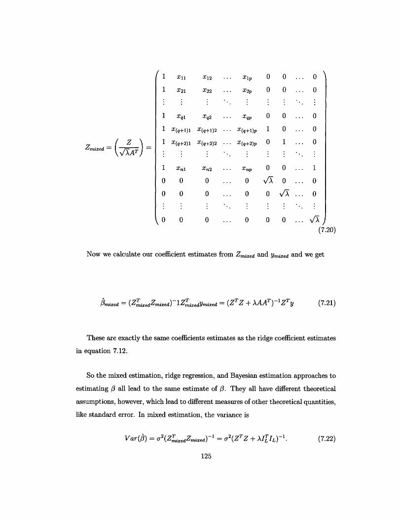
Zmixed ( (;AT
/Xll
X21
Xql
X(q+l)l
X(q+2)1
Xnl
0
0
0OO
x12
X22
Xq2
X(q+1)2
X(q+2)2
Xn2
0
0
0OO
... Xlp 0
... x 2p 0
.. Xqp 0
... X(q+l)p 1
... X(q+2)p 0
... Xnp 0
... o v
... 0 0... o o
o o
0
0
0
0
1
0
0
0
... 0
0
0
0
... o
1
.
... o
... · 0
(7.20)
Now we calculate our coefficient estimates from Zmixed and Ymixed and we get
(7.21)
These are exactly the same coefficients estimates as the ridge coefficient estimates
in equation 7.12.
So the mixed estimation, ridge regression, and Bayesian estimation approaches to
estimating /3 all lead to the same estimate of P. They all have different theoretical
assumptions, however, which lead to different measures of other theoretical quantities,
like standard error. In mixed estimation, the variance is
Var(3) = ,2 (Zi=edZmied) = 2(ZTZ + A IL)(Z,.~mi L)-i (7.22)
125
d = (edmized) zedYed = (Z + AA zT-'mixed - (4ZixedZmixed 1ixedYmixed = ( + AAA )-iy
I
j
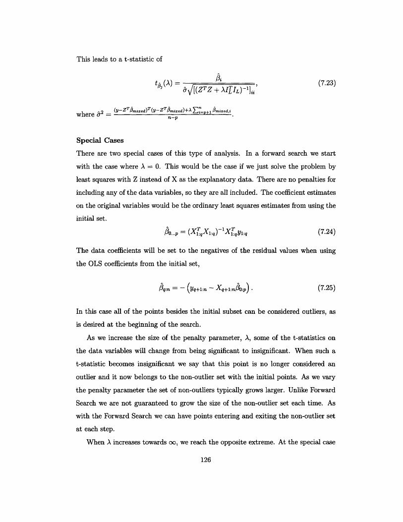
This leads to a t-statistic of
tpj (A) + AI[IL)' ]i (7.23)
where &2 = (y-zd) (y-Z mixed)+AZ=p+l mized,i
Special Cases
There are two special cases of this type of analysis. In a forward search we start
with the case where A = 0. This would be the case if we just solve the problem by
least squares with Z instead of X as the explanatory data. There are no penalties for
including any of the data variables, so they are all included. The coefficient estimates
on the original variables would be the ordinary least squares estimates from using the
initial set.
30.-p = (XqXi: q) Xl:qYl:q (7.24)
The data coefficients will be set to the negatives of the residual values when using
the OLS coefficients from the initial set,
q= -n (Yq+l:n - Xq+l:nfJo:p). (7.25)
In this case all of the points besides the initial subset can be considered outliers, as
is desired at the beginning of the search.
As we increase the size of the penalty parameter, A, some of the t-statistics on
the data variables will change from being significant to insignificant. When such a
t-statistic becomes insignificant we say that this point is no longer considered an
outlier and it now belongs to the non-outlier set with the initial points. As we vary
the penalty parameter the set of non-outliers typically grows larger. Unlike Forward
Search we are not guaranteed to grow the size of the non-outlier set each time. As
with the Forward Search we can have points entering and exiting the non-outlier set
at each step.
When A increases towards oo, we reach the opposite extreme. At the special case
126
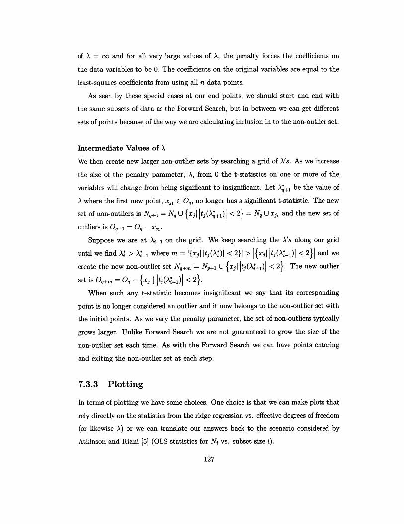
of A = oo and for all very large values of A, the penalty forces the coefficients on
the data variables to be 0. The coefficients on the original variables are equal to the
least-squares coefficients from using all n data points.
As seen by these special cases at our end points, we should start and end with
the same subsets of data as the Forward Search, but in between we can get different
sets of points because of the way we are calculating inclusion in to the non-outlier set.
Intermediate Values of A
We then create new larger non-outlier sets by searching a grid of A's. As we increase
the size of the penalty parameter, A, from 0 the t-statistics on one or more of the
variables will change from being significant to insignificant. Let Av+1 be the value of
A where the first new point, xj E Oq, no longer has a significant t-statistic. The new
set of non-outliers is Nq+l = Nq U {xj tj(Aq+l)I < 2} = Nq U xjl and the new set of
outliers is 0 q+1 = Oq- Xji.
Suppose we are at Ai-, on the grid. We keep searching the A's along our grid
until we find A > A* where m = {x3jl tj(A*) < 2}1 > {xj tj(A*_1 )l < 2}1 and we
create the new non-outlier set Nq+m = Np+1 U {xj |tj(A*+1) < 2}. The new outlier
set is Oq+m = Oq- {xj I tj(A*+1) < 2}.
When such any t-statistic becomes insignificant we say that its corresponding
point is no longer considered an outlier and it now belongs to the non-outlier set with
the initial points. As we vary the penalty parameter, the set of non-outliers typically
grows larger. Unlike Forward Search we are not guaranteed to grow the size of the
non-outlier set each time. As with the Forward Search we can have points entering
and exiting the non-outlier set at each step.
7.3.3 Plotting
In terms of plotting we have some choices. One choice is that we can make plots that
rely directly on the statistics from the ridge regression vs. effective degrees of freedom
(or likewise A) or we can translate our answers back to the scenario considered by
Atkinson and Riani [5] (OLS statistics for Ni vs. subset size i).
127

We consider this second case. For one, it allows us a direct comparison to the
Forward Search plots. Also given that all of the dummies have non-zero coefficients for
every A, the original variables' coefficients are artificially small in the ridge case. Some
shrinkage is desirable, as it is one of the main reasons for using ridge regression, but
with this many variables the shrinkage becomes somewhat excessive. Additionally,
the equivalent degrees of freedom 7.15 is problematically increased because the ridge
penalty tends to fit many non-zero "small" coefficients rather than forcing them to
zero. We don't choose to view insignificantly small coefficients as non-zero, so this
calculation does not correctly reflect our situation.
In the previous step, we found a number of different non-outlier sets, Np+l, Np+2,
... , N,. We now can calculate and plot all of the same OLS-type statistics (as in
Forward Search) for these non-outlier subsets. We then create similar plots to those
suggested for Forward Search. We will also suggest a few other plots to consider.
We also have the choice of how to measure tj(A), using the ridge regression view
or the mixed estimation view. There are merits to both viewpoints. They give us
very similar plots for the same data set, so there may not be too much reason to
labor over this choice. I will demonstrate this similarity with example data sets. We
recommend using the mixed estimation viewpoint in order to see the extreme points
of the plots.
7.3.4 Where to Look
Atkinson and Riani suggest that we study the plots for sharp changes in statistics.
These changes are an informal look at how the data is influencing our model and we
recognize their importance as well.
We also think that it is important to figure out which range of penalty parameters,
A, provide a good trade-off between the bias from including too many outliers and
the loss of efficiency due to omitting good observations. There are many suggestions
on how to choose A in the literature, but we will primarily consider prediction and
cross-validation. This idea has proved successful in a number of situations [17].
In [42], It was suggested that given that we have exerted some computational effort
128

to find an initial set of q good points, we decide to use them again to help us find a
good value for A. A cross-validation method was suggested, but this method was not
protected against leverage. Starting with the q points chosen from a high-breakdown
method like LMS help to protect us against leverage. By not adding dummy data
variables for these points we force the solution to fit these points more closely than
the points given dummy variables. Even though the dummy variables were added to
provide robustness with regard to vertical outliers, they are not effective for "bad"
leverage points. This becomes a problem in the suggested cross-validation method
because we remove one of the "good" points from the calculation in order to predict
it.
Once we remove a "good" point, we are no longer suggesting that the solution
should start close to the LMS solution, because with one fewer point, we cannot fully
define a regression line with the good points. This allows the "bad" leverage points
to have more influence on the values of the coefficient estimates for a given value of
A, than they do in the original fitting step. This hurts the comparison we are trying
to make by using the cross-validation step to choose a good A for the original fit.
Given this, we suggest a simple variation on the original suggestion for the cross-
validation step, do not include a dummy variable for the q + Ith "good" point. From
here we proceed as before. For each of the q good points and each value of A (from
our grid of As under consideration), we predict the good point observation using the
penalized regression coefficients for that given value of A which were calculated from
all of the data except for the point we are predicting. We then compare this prediction
to the real value to find a prediction residual. Again we use a robust measure of
prediction error (MAD) across the different prediction residuals for a given value of
A to find a robust prediction score for this value of A.
We could then choose the A that has the minimal prediction score. This minimal
prediction score will not necessarily correspond to best clean subset size. These
prediction scores are variable and it is possible that another larger subset size could be
chosen if we look at all subset sizes within some small deviation above this minimum
score. One rule suggested in [24] is that we should consider answers with a prediction
129

score within one standard deviation of the minimum.
One can calculate such a deviation by using the sub-scores that we calculate as a
part of the cross-validation. We measure the MAD of these sub-scores and scale this
variable to match the normality,
dev(A) = MAD(pscore(A))/.675. (7.26)
We then look for the largest subset size that corresponds to a prediction score less
than the minimum prediction score plus one deviation.
One-at-a-time cross-validation is known to be inconsistent in many situations, but
it is consistent when the number of predictors increases as n increases [39]. This is
true in our situation because our number of predictors is n + p which is proportional
to n.
We will also recommend some new plots based on these prediction residuals and
prediction scores in the next section.
7.4 Example: Hawkins Data
We are now going to look at a few examples of how the diagnostic traces from our
algorithm look when applied to various data sets.
7.4.1 Hawkins Data
We start with a synthetic data set known as the Hawkins data [25], which was also
featured in a demonstration of using Forward Search for regression problems [5]. The
Hawkins data has 128 observations (n=128), one outcome, and eight explanatory
variables (p=8). This data set was designed to contain masked outliers which would
difficult to find using least squares based diagnostics.
The first pair of plots we examine are the plots of subset size m vs. scaled OLS
residuals (Figure 7-7) and of subset size m vs. scaled squared OLS residuals (Figure
7-8). The residuals are scaled by the final estimate of of the error standard deviation
130
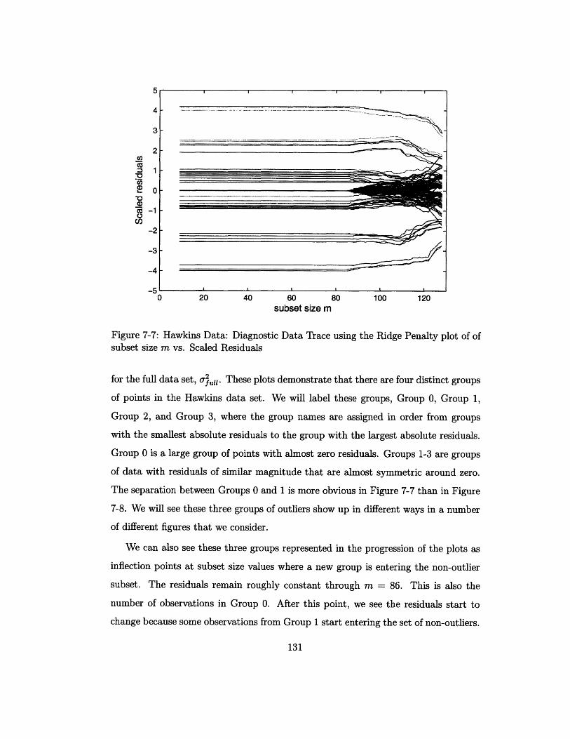
4
3
2cn
1
co -1
(n-2
-3
-4
_e-
0 20 40 60 80 100 120subset size m
Figure 7-7: Hawkins Data: Diagnostic Data Trace using the Ridge Penalty plot of ofsubset size m vs. Scaled Residuals
for the full data set, af,,l. These plots demonstrate that there are four distinct groups
of points in the Hawkins data set. We will label these groups, Group 0, Group 1,
Group 2, and Group 3, where the group names are assigned in order from groups
with the smallest absolute residuals to the group with the largest absolute residuals.
Group 0 is a large group of points with almost zero residuals. Groups 1-3 are groups
of data with residuals of similar magnitude that are almost symmetric around zero.
The separation between Groups 0 and 1 is more obvious in Figure 7-7 than in Figure
7-8. We will see these three groups of outliers show up in different ways in a number
of different figures that we consider.
We can also see these three groups represented in the progression of the plots as
inflection points at subset size values where a new group is entering the non-outlier
subset. The residuals remain roughly constant through m = 86. This is also the
number of observations in Group 0. After this point, we see the residuals start to
change because some observations from Group 1 start entering the set of non-outliers.
131
r,.. .. ..... ... .. ..... ... . ........... ...... .. .. ..... ........ .. .......
. .... .. .............. . ............... ..... ..
I t
. - J ___ . I I
20
18
16
c 14
) 12
-0()- 10C'
'0
o 6
4
2
n
0 20 40 60 80 100 120subset size m
Figure 7-8: Hawkins Data: Diagnostic Data Trace using the Ridge Penalty plot ofsubset size m vs. Squared Scaled Residuals
132
In Figure 7-7, we can see that the residuals on the observations in Group 0 start
growing and continue growing as the different groups of outliers are added. In fact
when considering the full data set (m=128), some of the observations in Group 0 now
have residuals larger than observations in Groups 1 and 2.
In contrast, the residuals on the other groups are generally decreasing. The resid-
uals on Group 1 seem to decrease steadily from m = 87 to m = 128. The residuals
on Group 2 seem to increase slightly while the observations in Group 1 are added to
the non-outlier set, but they decrease after m = 110 when the observations in Groups
2 and 3 get added to the non-outlier set. The residuals for Group 3 decrease slowly
from m = 86 through m = 122, but decrease sharply when the observations in Group
3 finally enter the non-outlier subset.
The OLS solution corresponds to m = 128 on these plots. We can see that
Groups 0 - 2 are no longer distinct when it comes to the residual plots. Many of the
observations in Group 0 have become swamped. Only the six observations in Group
3 appear to be outliers. We can also see that with a subset size as large as m = 120,
Group 2 can be seen as distinct from Groups 0 and 1.
Another interesting and new plot to consider is the plot of just the residuals from
the initial subset of "good" points,
i - zXT$m) (7.27)
'full
for all i E I*, as the subset size, m, increases. This is one of the new plots we suggest
in [42]. An example for the Hawkins data can be seen in Figure 7-9. We can see that
as the outlier groups begin entering at m = 87, these residuals start dramatically
increasing. None of them are larger than two, but they are very different from their
values in the range m = 9 to m = 87. Also &full is inflated by the outliers.
This last plot gives us some idea of what might be happening with prediction of
the clean data as outliers are added to the set used to fit the parameters. Traditionally
we prefer to not include a point in the set of points used to fit the parameters we are
using to predict it, for the many reasons we have already discussed. The next new
133
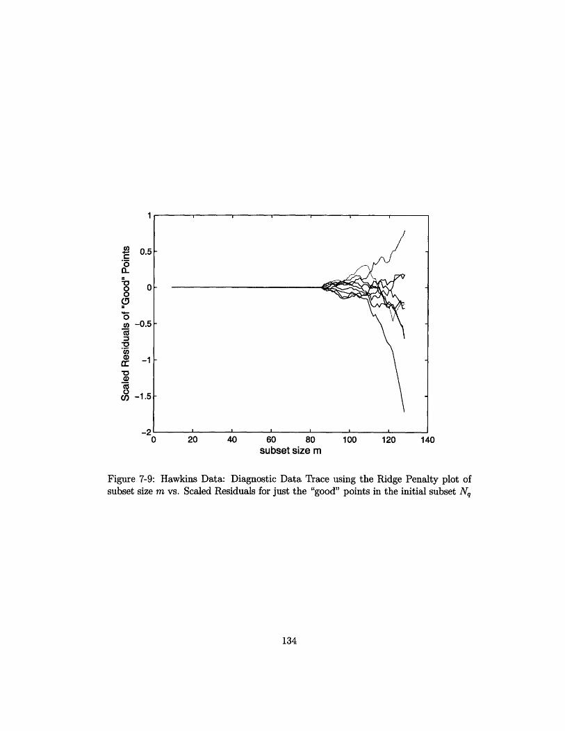
1
- 0.5
o 0o
Wo0an -0.5
u-n" -1
a)
0cU -1.5
I,0 20 40 60 80 100 120 140
subset size m
Figure 7-9: Hawkins Data: Diagnostic Data Trace using the Ridge Penalty plot ofsubset size m vs. Scaled Residuals for just the "good" points in the initial subset Nq
134

plot we suggest is a plot of the prediction residuals that we calculated while trying
to discover a good value of A as a function of the subset size m suggested for this
value of A. For an example of this see Figure 7-10. There is likely to be more than
one prediction residual value for each subset size because models of a given size can
result from more than one value of A. In these cases a vertical line between the lowest
and highest prediction residuals will be plotted. We can also plot a variation on this
where we plot the prediction scores as a function of its corresponding subset size. For
an example of this see Figure 7-11.
Once again in both of these plots, we can see how the introduction of the different
outlier groups affects our results. The prediction residuals are constant through m =
86. We see jumps in the plots when the different outlier groups enter the non-outlier
subset. Once again the first drastic change occurs at m = 86. The change is large
enough that our one deviation rule from Section 7.3.4 suggests that this is the subset
size that we should consider as the largest set of clean points.
This is actually a different suggestion than the one mentioned in [42]. This is
because in that examination we did not consider a comprehensive enough grid of A's.
In that case, we observed a local minimum at A : .02 which was what was reported
This leads to a subset size of m = 90.
A better measure of the local minimum can be seen in Figure 7-11 and in another
new figure we suggest, Figure 7-12, which were made with a more comprehensive grid
of A's. These plots demonstrate that the local minimum is actually at m = 93 and
logl0 A -1.59 (A .025) .
This new plot we consider is the prediction score we calculated for each value of A
as a function of logl0 A. This plot better captures the continuous nature of the change
in the prediction score. An example of this plot for the Hawkins data can be seen in
Figure 7-12.
In Figure 7-12, we see a general S-shaped plot with an increasing prediction score
as A increases. We also see two features that appeared in Figure 7-11 where there is
an increase and then a slight downturn in the score, leading to two local minima. The
beginning of the period of general increase in prediction score occurs at A .003.
135
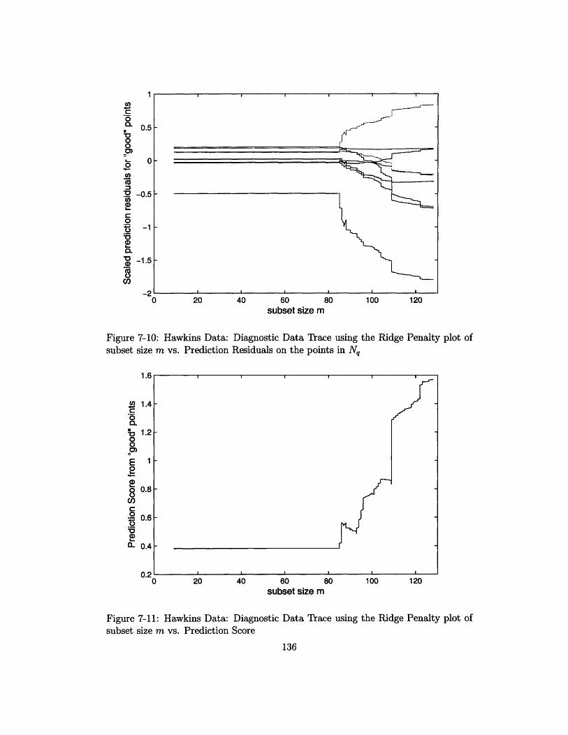
20 40 60 80 100 120subset size m
Figure 7-10: Hawkins Data: Diagnostic Data Trace using the Ridge Penalty plot ofsubset size m vs. Prediction Residuals on the points in Nq
20 40 60 80 100 120
subset size m
Figure 7-11: Hawkins Data: Diagnostic Data Tracesubset size m vs. Prediction Score
136
using the Ridge Penalty plot of
1
0.5
0
-r0o
a
'a=
o
'a
am
coC.)
-0.5
-1
-1.5
-20
1.6
n 1.4Co-0o.- 1.200
E 1
a)o 0.8C)C
0.6
L 0.4
no0
· · · ·
I I I I I I
I
r
I
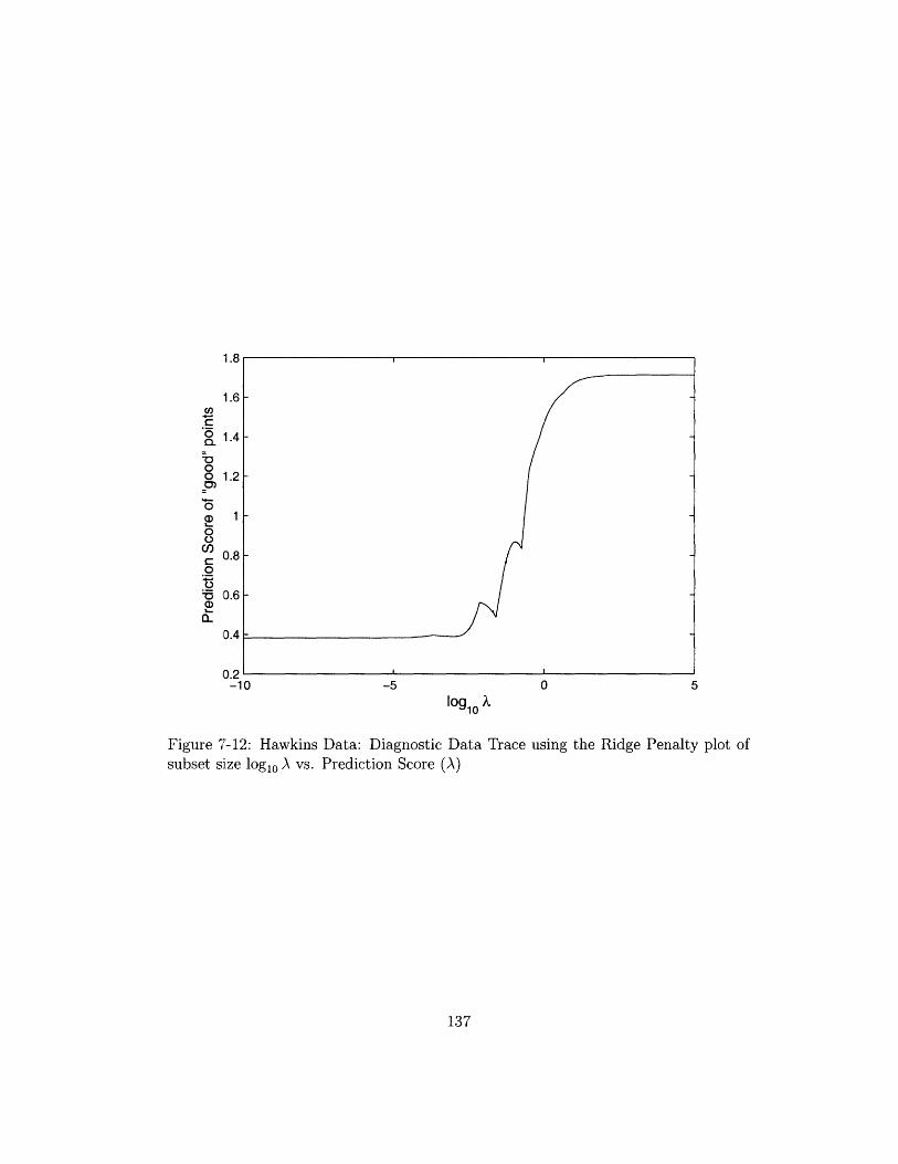
o 1
o-C01o,
o
o00-) o0
.,a0
ID
-10 -5 0 5
I10lo X
Figure 7-12: Hawkins Data: Diagnostic Data Trace using the Ridge Penalty plot ofsubset size log10 A vs. Prediction Score (A)
137
1 r
1
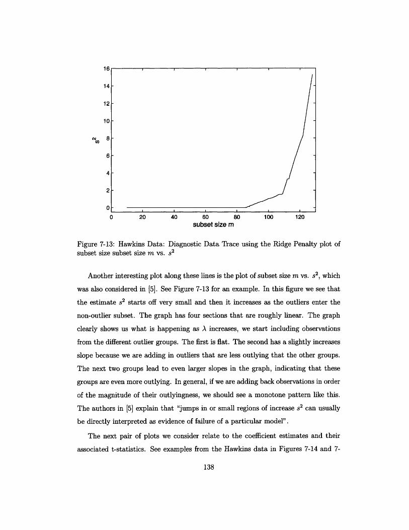
14
12
10
CY 8O~
6
4
2
I.U
0 20 40 60 80 100 120subset size m
Figure 7-13: Hawkins Data: Diagnostic Data Trace using the Ridge Penalty plot ofsubset size subset size m vs. s2
Another interesting plot along these lines is the plot of subset size m vs. s2, which
was also considered in [5]. See Figure 7-13 for an example. In this figure we see that
the estimate s2 starts off very small and then it increases as the outliers enter the
non-outlier subset. The graph has four sections that are roughly linear. The graph
clearly shows us what is happening as A increases, we start including observations
from the different outlier groups. The first is flat. The second has a slightly increases
slope because we are adding in outliers that are less outlying that the other groups.
The next two groups lead to even larger slopes in the graph, indicating that these
groups are even more outlying. In general, if we are adding back observations in order
of the magnitude of their outlyingness, we should see a monotone pattern like this.
The authors in [5] explain that "jumps in or small regions of increase s2 can usually
be directly interpreted as evidence of failure of a particular model".
The next pair of plots we consider relate to the coefficient estimates and their
associated t-statistics. See examples from the Hawkins data in Figures 7-14 and 7-
138
14 · · · 1AI11
I I I I I I
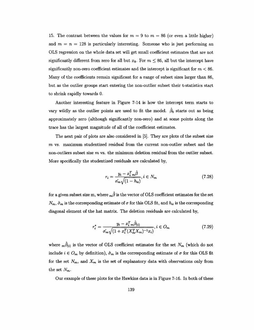
15. The contrast between the values for m = 9 to m = 86 (or even a little higher)
and m = n = 128 is particularly interesting. Someone who is just performing an
OLS regression on the whole data set will get small coefficient estimates that are not
significantly different from zero for all but x8. For m < 86, all but the intercept have
significantly non-zero coefficient estimates and the intercept is significant for m < 86.
Many of the coefficients remain significant for a range of subset sizes larger than 86,
but as the outlier groups start entering the non-outlier subset their t-statistics start
to shrink rapidly towards 0.
Another interesting feature in Figure 7-14 is how the intercept term starts to
vary wildly as the outlier points are used to fit the model. /0 starts out as being
approximately zero (although significantly non-zero) and at some points along the
trace has the largest magnitude of all of the coefficient estimates.
The next pair of plots are also considered in [5]. They are plots of the subset size
m vs. maximum studentized residual from the current non-outlier subset and the
non-outliers subset size m vs. the minimum deletion residual from the outlier subset.
More specifically the studentized residuals are calculated by,
Y= i Xi m E N (7.28)m ri /1 -
for a given subset size m, where m: is the vector of OLS coefficient estimates for the set
Nm, am is the corresponding estimate of u for this OLS fit, and hii is the corresponding
diagonal element of the hat matrix. The deletion residuals are calculated by,
Yi - Xi m(i)(7.29)
om/(1 + XiT(XmXm)t -xi)
where m(i) is the vector of OLS coefficient estimates for the set Nm (which do not
include i E Om by definition), am is the corresponding estimate of ur for this OLS fit
for the set Nm, and Xm is the set of explanatory data with observations only from
the set Nm.
Our example of these plots for the Hawkins data is in Figure 7-16. In both of these
139
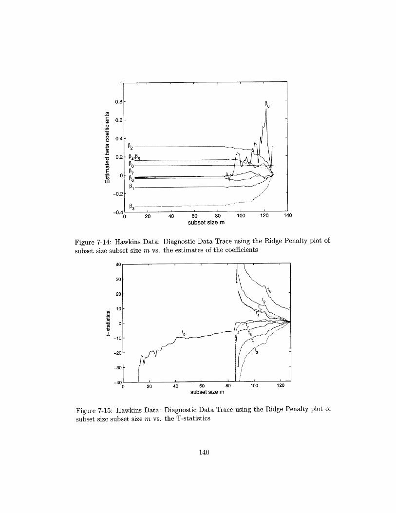
.a,
f)o0C.)
.0a)
E
W
0 20 40 60 80 100 120 140subset size m
Figure 7-14: Hawkins Data: Diagnostic Data Trace using the Ridge Penalty plot of
subset size subset size m vs. the estimates of the coefficients
20 40 60 80 100 120subset size m
Figure 7-15: Hawkins Data: Diagnostic Data Tracesubset size subset size m vs. the T-statistics
using the Ridge Penalty plot of
140
40
30
20
u)o
.
10
0
-10
-20
-30
-AN0
-UI .'

plots, we can see three distinct local maxima corresponding to the different outlier
groups. In the maximum studentized residual plot, we see that once we include
the first outlier in the non-outlier subset, there is a very large maximum studentized
residual (> 8). As more of the outliers from this outlier group get added the maximum
studentized residual decreases. We see this same pattern for each of the next two
outlier groups. The final maximum studentized residual at m = n = 128 is 3.0. This
is large, but not terribly extreme as this is the maximum of 128 observations. This
is also much lower than the value we would have seen if we included fewer points of
this outlier group in the final fit.
This plot demonstrates the problem of outlier masking. If we use studentized
residuals from the full data set to help us look for outliers we will not discover that
we have outliers in this set. This type of diagnostic trace allows us to examine this
statistic at multiple points to see a fuller picture.
In the minimum deletion residual plot, we see a very extreme value just before the
first outlier enters the non-outlier set. In order to show other details on this plot, we
capped the value shown at 20, but the maximum is actually reached at 92.0, which
shows you how extreme the other observations looked compared to Group 0. Once
again we see that as more observations enter the values decrease to unremarkable
values. This pattern again repeats itself for Groups 2 and 3.
This plot shows you the limitations of deletion-based outlier detection methods
when there are groups of outliers. Once we have added a large enough group of
outliers, deleting just one of two of then will not give you a deletion residual that
looks large enough to provide evidence of outlying points.
A final plot considered in [5] is a plot of the leverage of each point (in the form
of the hat matrix diagonals) as a function of subset size. This plot should show us if
there is any evidence of leverage in the different subsets. In the case of the Hawkins
data, the plot looks rather unremarkable indicating that there is little evidence of
leverage in the various subsets. See Figure 7-17.
141
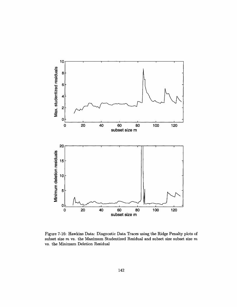
10
0 20 40 60 80subset size m
100 120
20
.t
am
E
EE._
15
10
5
00 20 40 60 80 100 120
subset size m
Figure 7-16: Hawkins Data: Diagnostic Data Traces using the Ridge Penalty plots ofsubset size m vs. the Maximum Studentized Residual and subset size subset size mvs. the Minimum Deletion Residual
142
uC)
a)-
CO
NCa)e-
C)
8
6
4
2
0
· · ·
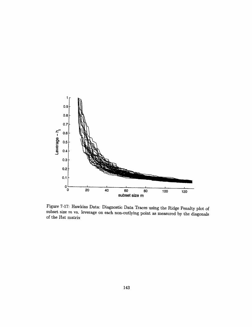
,=
0I
a)
u 20 , vsubset size m
Figure 7-17: Hawkins Data: Diagnostic Data Traces using the Ridge Penalty plot ofsubset size Tm vs. leverage on each non-outlying point as measured by the diagonalsof the Hat matrix
143
I
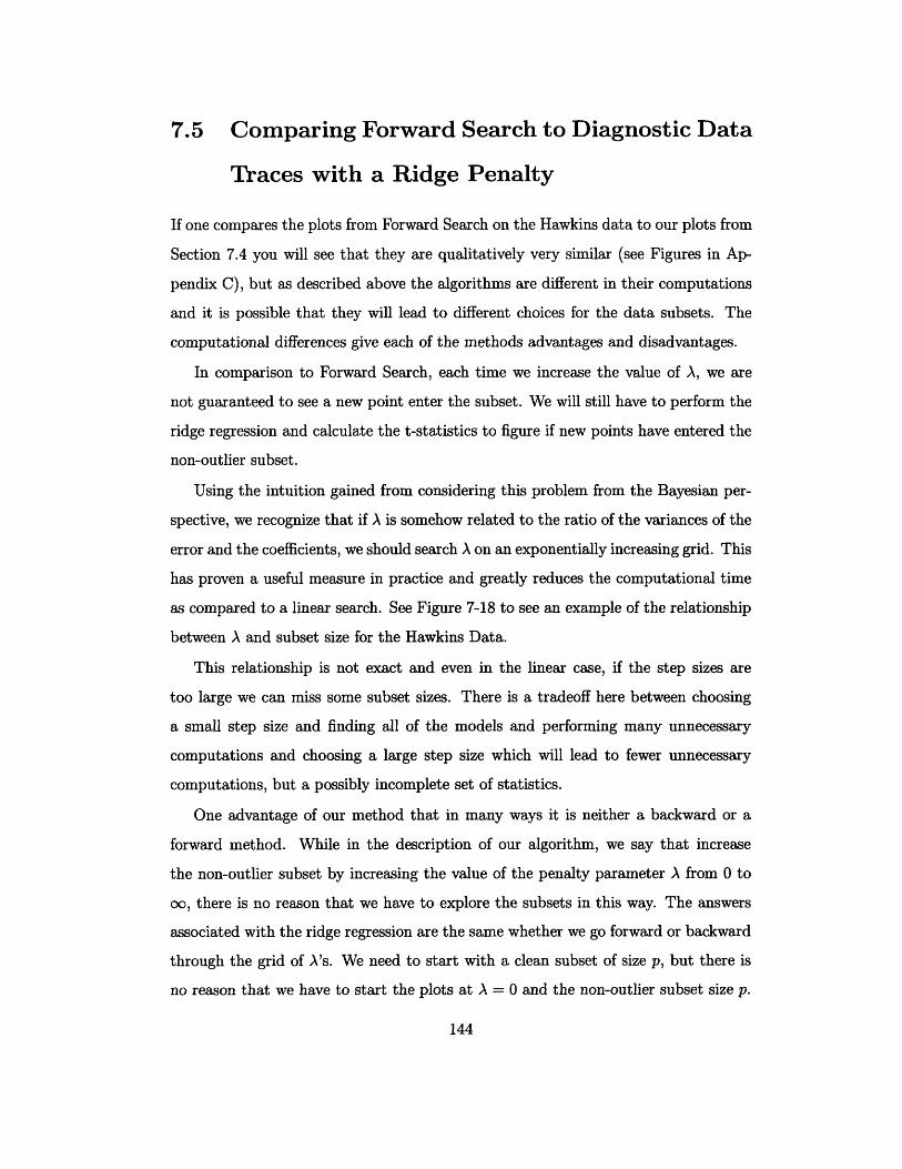
7.5 Comparing Forward Search to Diagnostic Data
Traces with a Ridge Penalty
If one compares the plots from Forward Search on the Hawkins data to our plots from
Section 7.4 you will see that they are qualitatively very similar (see Figures in Ap-
pendix C), but as described above the algorithms are different in their computations
and it is possible that they will lead to different choices for the data subsets. The
computational differences give each of the methods advantages and disadvantages.
In comparison to Forward Search, each time we increase the value of A, we are
not guaranteed to see a new point enter the subset. We will still have to perform the
ridge regression and calculate the t-statistics to figure if new points have entered the
non-outlier subset.
Using the intuition gained from considering this problem from the Bayesian per-
spective, we recognize that if A is somehow related to the ratio of the variances of the
error and the coefficients, we should search A on an exponentially increasing grid. This
has proven a useful measure in practice and greatly reduces the computational time
as compared to a linear search. See Figure 7-18 to see an example of the relationship
between A and subset size for the Hawkins Data.
This relationship is not exact and even in the linear case, if the step sizes are
too large we can miss some subset sizes. There is a tradeoff here between choosing
a small step size and finding all of the models and performing many unnecessary
computations and choosing a large step size which will lead to fewer unnecessary
computations, but a possibly incomplete set of statistics.
One advantage of our method that in many ways it is neither a backward or a
forward method. While in the description of our algorithm, we say that increase
the non-outlier subset by increasing the value of the penalty parameter A from 0 to
oo, there is no reason that we have to explore the subsets in this way. The answers
associated with the ridge regression are the same whether we go forward or backward
through the grid of A's. We need to start with a clean subset of size p, but there is
no reason that we have to start the plots at A = 0 and the non-outlier subset size p.
144
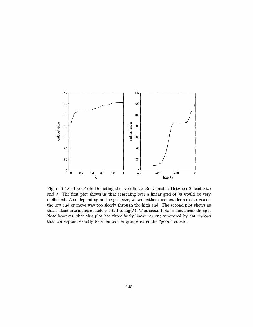
140
120
100
a).N 80
U,
= 60cn
40
20
n
U)NU)
U,
.0U,
0 0.2 0.4 0.6 0.8 1 -30 -20 -10 0X log(X)
Figure 7-18: Two Plots Depicting the Non-linear Relationship Between Subset Sizeand A: ':rhe first plot shows us that searching over a linear grid of As would be veryinefficient. Also depending on the grid size, we will either miss smaller subset sizes onthe low end or move way too slowly through the high end. The second plot shows usthat subset size is more likely related to log(A). This second plot is not linear though.Note however, that this plot has three fairly linear regions separated by fiat regionsthat correspond exactly to when outlier groups enter the "good" subset.
145
1
F
v

We can choose to just try to find the traces for a range of subset sizes. For instance
in many cases we believe there is less than 50% contamination in our data. We could
restrict our plots to n/2 to n in this case by starting the search with values of A large
enough.
(Note: Sometimes more than one value of A corresponds to the same subset size.
We choose the answer corresponding to the smallest value of A, so in some sense,
one may view this as a forward perspective. This however does not prevent us from
searching any grid of penalty parameters in any direction.)
Undertaking such a search has its own challenges in that we do not know a priori
which A's correspond to which subset sizes, as stated above. We can however search
a coarse grid to determine an interesting region to search. We are likely to do this
anyway in the standard version of our algorithm to determine the maximum value of
A to consider to get the final subset size of A.
Another advantage here is that if we decide to start with only computing the
second half of the chart, we can always add the rest later because the computations
can be done independently. This leads us to another advantage, the values for the
plots can be generally computed in parallel. There are some advantages to using
insertion or deletion ideas to speed up the computation of the OLS statistics, some
of which will be lost if we move to a parallel computing setting. In the parallel
setting we can still use these ideas, but we would always have to start with a full OLS
computation for the first subset we find.
Even without these somewhat complex computational maneuvers, we find that
the Diagnostic Traces with the Ridge Penalty calculations are faster to compute that
the Forward Search calculations. We compared the CPU time required for each set
of calculations and we found that our algorithm was by far faster, 41.409 seconds vs.
414.386 seconds. See Table B.2.
Forward Search boasts that the choice of initial subset is not as important as it
may seem because often suboptimal choices can be overcome. This is because in their
algorithm, unlike ours, the points in the initial subset can leave the set of non-outliers.
We could alter our algorithm to allow the initial points to leave the non-outlier subset.
146

What one would do is add dummies for these variables, but make it more expensive
for one to choose these points as outliers. This can be accomplished by scaling their
dummies down to require larger coefficients to fit the same size residual of one of the
other points. This way we indicate a prior belief that the initial points are "good",
but we no longer require them to be non-outliers. We only require that there be
sufficient evidence for them to leave the subset.
We can use this type of scaling to include prior information about other data points
as well. We caution the use of this for points other than the original data because the
whole reason we are using this method to find information about outliers. We don't
want to use the method to confirm previously supposed incorrect information.
7.6 Example: The Rousseeuw Data
The next two data sets we consider are two simple one-dimensional data sets discussed
by Rousseeuw and Leroy [51]. They have become standard benchmark data sets for
robust methods in regression, whether it be estimation or outlier detection. The first
set, the Belgian Phone Data, is a good demonstration of vertical outliers. The second,
the Hertzsprung-Russell Star Data, is a good example of bad leverage points.
These data sets are useful because we need to at least demonstrate that a method
works in a simple case that has an easily verifiable answer. Each of these data sets
only has one explanatory variable, so it would be easy for anyone to just look at a
scatter plot and identify the outliers. Other researchers have said that methods that
fail on these cases will most likely never gain widespread use [22]. Fortunately, we
are successful in identifying the outlying points in each case.
7.6.1 The Belgian Phone Data
This data set is a record of the number of international phone calls from Belgium,
taken from the Belgian Statistical Survey, published by the Ministry of Economy.
The outcome variable, y, is the number of phone calls. The explanatory variable, x,
is the year, indicating that the number of international phone calls was increasing
147
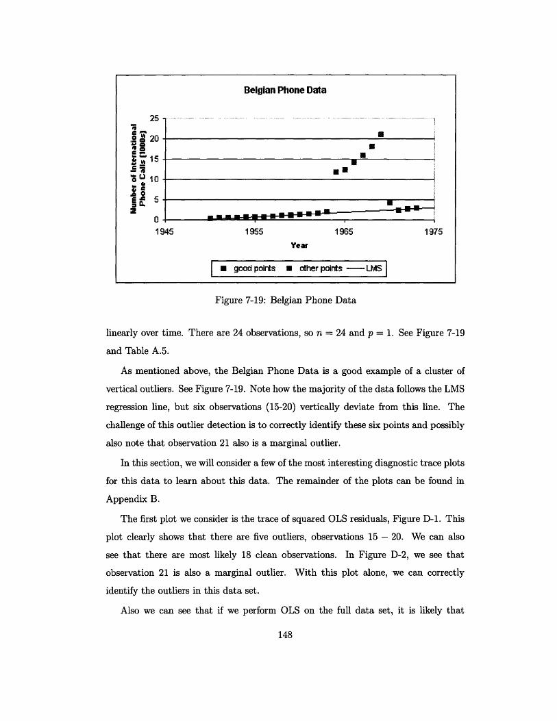
Belgian Phone Data
Figure 7-19: Belgian Phone Data
linearly over time. There are 24 observations, so n = 24 and p = 1. See Figure 7-19
and Table A.5.
As mentioned above, the Belgian Phone Data is a good example of a cluster of
vertical outliers. See Figure 7-19. Note how the majority of the data follows the LMS
regression line, but six observations (15-20) vertically deviate from this line. The
challenge of this outlier detection is to correctly identify these six points and possibly
also note that observation 21 also is a marginal outlier.
In this section, we will consider a few of the most interesting diagnostic trace plots
for this data to learn about this data. The remainder of the plots can be found in
Appendix B.
The first plot we consider is the trace of squared OLS residuals, Figure D-1. This
plot clearly shows that there are five outliers, observations 15 - 20. We can also
see that there are most likely 18 clean observations. In Figure D-2, we see that
observation 21 is also a marginal outlier. With this plot alone, we can correctly
identify the outliers in this data set.
Also we can see that if we perform OLS on the full data set, it is likely that
148
2 5 . ............. .. .... ................. . .. ......... ... ............ .......... ............................ .. .................................... ....... ............ ..................... .... ........................... 2 5
20
4 ' 15
a 10- l
oA 5z1945 1955 1965 1975
Year
good points M other points - LMS
I
1
u)
co-Ir
2aoI)
()'o242322
0 5 10 15 20subset size m
Figure 7-20: Belgian Phone Data: Diagnostic Trace from Ridge Penalty
some outliers will be missed and three other "clean" points will have larger squared
residuals than some of the outliers.
There are other figures that help us to identify these same points. These include
the spikes we find in the maximum studentized residual and minimum deletion resid-
uals plots, Figure D-5. The plot of the coefficient estimates and t-statistics, Figure
D-6, is also fairly straight forward to interpret. The coefficient estimates remain very
flat until the outliers are included.
As is often the case, identifying the outliers is a useful first step in understanding
why these points deviate from the general pattern in the first place. In the case of this
data set, it was learned upon closer examination of the data collection methods that
during the years of 1964-1969 (15-20) and the beginning of 1970 (21), the number of
minutes of international phone calls was recorded rather than the number of calls.
Inconsistent data collection methods is one of the many popular reasons that a data
set can have outliers.
149
1_
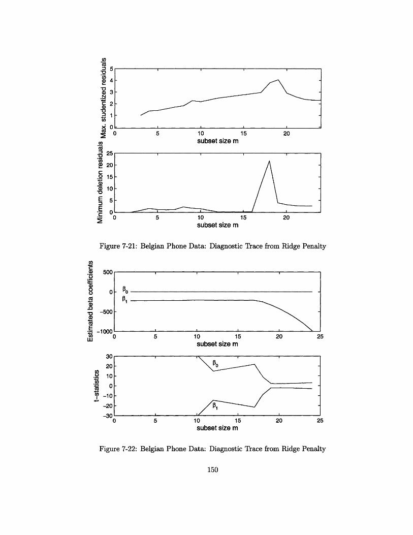
5 10
subset size m15 20
5 10 15 20
subset size m
Figure 7-21: Belgian Phone Data: Diagnostic Trace from Ridge Penalty
0 5 10 15 20 2!
subset size m
) g sx f~~~~~~~~~~~~3
5 10 15subset size m
20
5
25
Figure 7-22: Belgian Phone Data: Diagnostic Trace from Ridge Penalty
150
U)
5
a) 3Nc 2a)
Cd-0 0
"a ,NP
2.o 1
a. 1
E
E
, - _ _ I _ _ _ _ ~ -i I i
0
.o
8
Oan'aE
W
50C
C
-50C
-10OC
,.
?,a,Ij
3C
2C
10
C
-1C
-2C
-3C0
·
uvn

7.6.2 The Hertzsprung-Russell Star Data
This data set is an example of a Hertzsprung-Russell (H-R) star data set used to
make a Hertzsprung-Russell star diagram. Such diagrams are scatter plots of a star's
luminosity vs. its temperature (equivalently color (Hertzsprung) or spectral type
(Russell)) on a log scale.
This particular H-R star data set is from the Star Cluster CYG OB1. The outcome
variable, y, is log intensity and the explanatory variable, x, is log temperature. There
are 47 observations, so n = 47 and p = 1. See Figure 7-23 and Tables A.6 and A.7.
In Figure 7-23, we can see that there is a general linear trend for the bulk of the
data with four very bad and two fairly bad leverage points as well as a few marginal
vertical outliers. What makes this data set so challenging to work with is that there
is a lot of variance among the "good" points and this variance is not much lower than
the variance estimate we get if we fit the all the points (including the "bad" leverage
points) in an OLS.
The first plot that we usually consider is the plot of the scaled squared residuals,
Figure 7-25. From this plot is is clear that observations 11, 20, 30, and 34 are outliers
and that they are possibly a cluster. They each have extremely large squared scaled
residuals until observation 11 enters the model at subset size 44, at which time they
all are fit fairly well, with small residuals. If we zoom in at the end of the plot (see
Figure ??), we see that the residuals on the rest of the observations all increase at
the end, some to values larger than those on observations 11, 20, 30, and 34.
We also note that observations 7 and 9 have larger residuals that the other points,
besides 11, 20, 30, and 34. Until subset size 18 both 7 and 9 have significant residuals.
It is just after this point that observation 7 enters the non-outlier subset, which drives
its residual (and those of observations 11, 20, 30 and 34) down dramatically. This
indicates that both observations 7 and 9 are points of interest.
We can also examine leverage issues using the subset size vs. hat diagonals plot.
In Figure 7-26, we see that unlike the Hawkins Data and the Belgium Phone Data,
leverage is finally an issue with this data set. We knew this by looking at the scatter
151
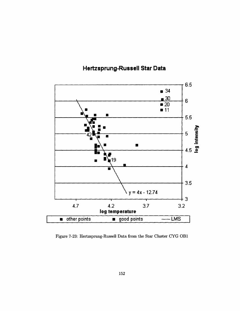
Hertzsprung-Russell Star Data
4.7 4.2 3.7
6.5
5.5
4
3.5
3
3.2log temperature
other points * good points -- LMS
Figure 7-23: Hertzsprung-Russell Data from the Star Cluster CYG OB1
152
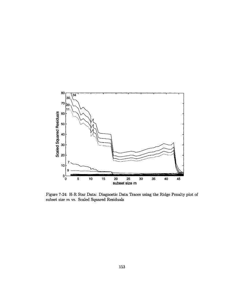
a)
a)r-O
a,
cn
C,,
0 5 10 15 20 25 30 35 40 45subset size m
Figure 7-24: H-R Star Data: Diagnostic Data Traces using the Ridge Penalty plot ofsubset size m vs. Scaled Squared Residuals
153
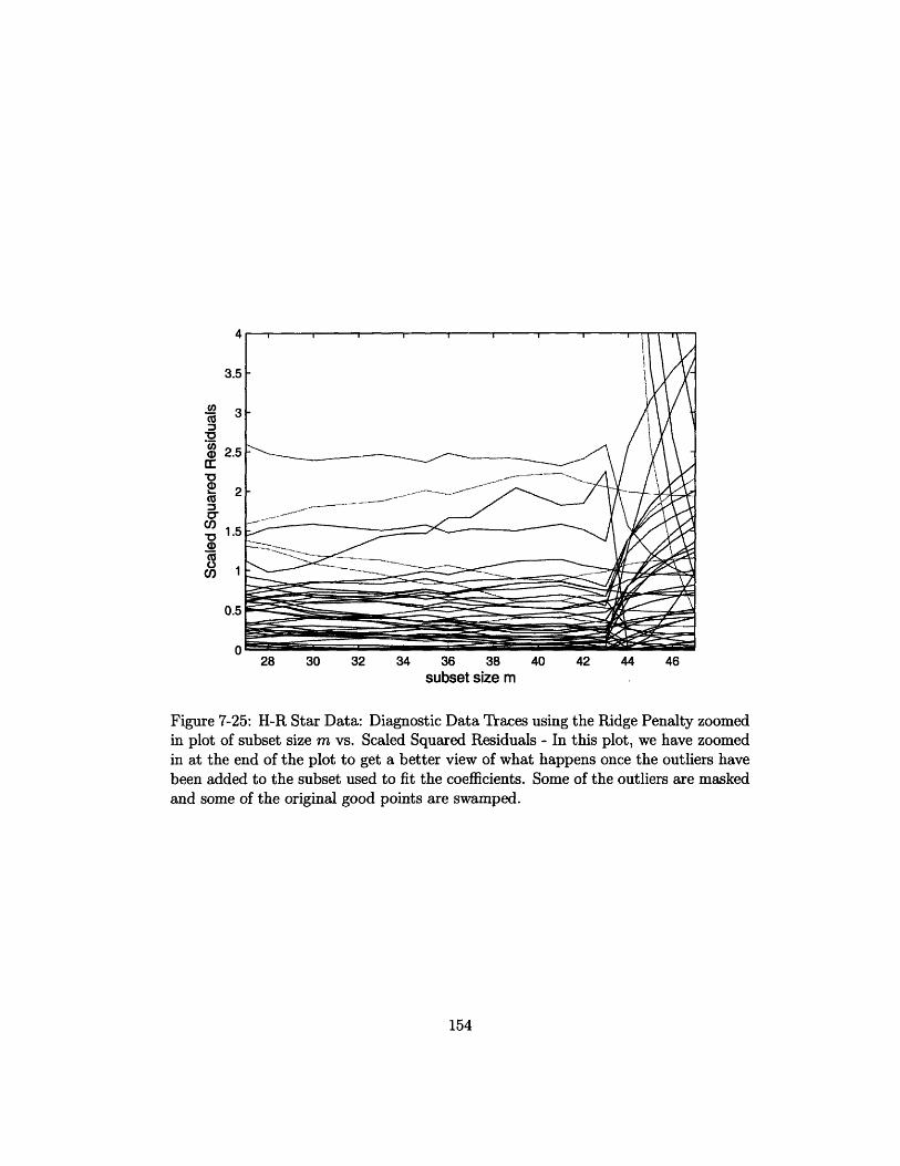
3
*0
a, 2
Er-aCuc3() 1"o
Cuco
O)
0
28 30 32 34 36 38 40 42 44 46subset size m
Figure 7-25: H-R Star Data: Diagnostic Data Traces using the Ridge Penalty zoomedin plot of subset size m vs. Scaled Squared Residuals - In this plot, we have zoomedin at the end of the plot to get a better view of what happens once the outliers havebeen added to the subset used to fit the coefficients. Some of the outliers are maskedand some of the original good points are swamped.
154
A

plot, but this plot shows us how the Leverage plot looks when there are leverage
points. On the far right we see the four main bad leverage points, observations 11,
20, 30 and 34, enter the subset and they all have high leverage. As each new point
enters the hat diagonal values decrease for these points because there are now more
points in this region of the x values.
This plot also leads us to believe that observations 7 and 14 are interesting points
that definitely have issues with leverage. Whether or not they are bad leverage points
is not entirely clear from this plot alone, but the plots suggest that we examine these
points more closely.
The entrance of observations 7 and 14 into the model correspond to areas of
decrease in the scaled squared OLS residuals for observations 11, 20, 30, and 34
as can be seen in Figure 7-25. These decreases make those four points look less
outlying, but their values were so extreme that they are still obviously outliers. This
is a possible indication that points 7 and 14 are not good outliers.
In Figure 7-27, we see the characteristic spikes in our plots of the maximum
studentized residual and the minimum deletion residual when the four outliers enter
at the end of the trace. There is also a feature in the middle corresponding to
observation 7 entering the model. Observation 7 was one of the other less drastic bad
leverage points. We find that perhaps this observation is being added to the non-
outlier set too soon, but when it was added there was an indication that a possible
outlier was being added to the set.
Unfortunately we note from these graphs that using the ridge penalty is not getting
us an entirely ideal set of subsets. We see that observation 7 comes into the non-
outlier subset too soon. While we can still tell from the plot that this observation is
troublesome and we can still recognize the 4 main outliers, we would prefer this point
to enter the non-outlier subset at a later point.
These data can be best understood in terms of the true model for this data.
Physical models for stars tell us that the luminosity for a object emitting thermal
radiation L - R2T4 or equivalently log L 2 log R + 4 log T. The coefficient of 4
on logT turns out to exactly match the coefficient estimate for the LMS solution.
155
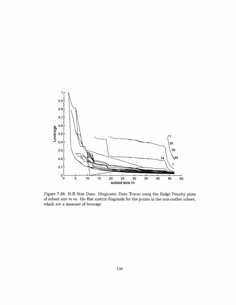
a)
a)CD-j
0 5 10 15 20 25 30 35 40 45 50subset size m
Figure 7-26: H-R Star Data: Diagnostic Data Traces using the Ridge Penalty plotsof subset size m vs. the Hat matrix diagonals for the points in the non-outlier subset,which are a measure of leverage
156
4
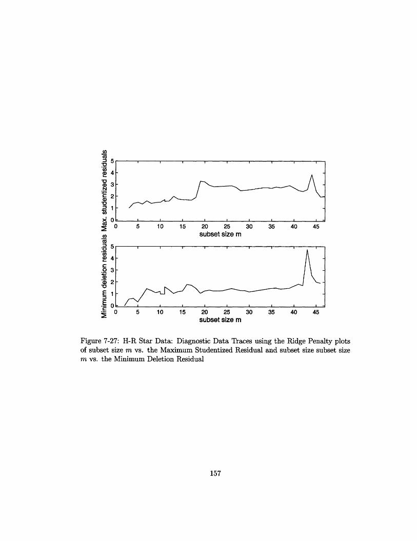
5 10 15 20 25
subset size m
10 15 20 25
subset size m
30 35 40 45
30 35 40 45
Figure 7-27: H-R Star Data: Diagnostic Data Traces using the Ridge Penalty plotsof subset size m vs. the Maximum Studentized Residual and subset size subset sizem vs. the Minimum Deletion Residual
157
0
c)
- 5
-oC43
C 2()o
V0
60
'o._
C0a)
E
EC -
0 5
_ ·
· · · · ·
I
I I I I I ~ I I -
The term associated with the radius was lumped into the intercept here, but this is
incorrect because the stars actually have varied radii. The "outliers" turn out to just
be stars with substantially larger radii, so they have a different value for log R than
the bulk of the stars which are all of similar size.
This data is also an example of how robust methods can teach us about our data.
Robust methods are not all about ignoring outlying observations. They can help
us to identify outlying observations. We can then try to learn what makes these
observations different and hopefully help us to build a better model.
7.7 Diagnostic Data Traces Using LARS
Once again we can change the penalty function in our algorithm, in fact all we need
at any given point is a method to describe which of the n points are not selected, and
thus not outliers. Many of the original advantages to using the LARS algorithm for
selection are seen again in this application. We have the sparsity which makes deter-
mining which points are in the subset at a given point easier. The LARS algorithm
also tells us exactly where the breakpoints are in the parameterized optimization path,
so we no longer need to use the time intensive and possibly imperfect grid method.
The computational speed of the LARS algorithm makes up for the fact that we can
no longer use parallel computations, as in the algorithm using the ridge penalty. In
fact, algorithm for creating diagnostic data traces using LARS is by far the fastest of
the three algorithms (Forward Search, Diagnostic Data Traces using Ridge Penalty,
and Diagnostic Data Traces using LARS) when performed on example data sets. See
Table B.2.
One drawback of using the LARS algorithm is that it is not designed to adjust
the penalties on the different variables, like we could with the ridge penalty param-
eter. Specifically, the LARS algorithm does not allow us to not penalize the original
variables as we did when using the ridge penalty. If we used the traditional methods
to fit the LASSO solutions, it is possible to accommodate having no penalty on the
original variables, but these estimation procedures are much more computationally
158

intensive. This means that, if we choose to use the LARS algorithm, the original
variables will not be protected from being deselected.
(Note: It may be possible to alter the LARS algorithm to perform the desired
estimation procedure, but that is outside of the defined scope of this thesis.)
From here we see three ways to proceed:
1. We allow all of the original variables, including the intercept, to compete along
with the dummies for selection. This means that all variables are eligible to be
shrunk or selected.
2. WVe can remove the intercept from the estimation procedure as in previous chap-
ters by centering all of the variables including the outcome variable. We choose
to use robust estimators to center the original variables and the mean to center
the dummies.
3. We use the LMS estimate for the intercept to estimate the intercept. We then
subtract this from the outcome variable similarly to what is described in [14]
when describing the "main effects first" variation. We still choose to include a
variable representing the intercept in this option to accommodate variation in
the value of the intercept in case our original choice was grossly incorrect.
Of the three methods, we recommend Method 3. Method 1 is similar to how we
set up the data when using the ridge penalty. The problem with this method is that
we cannot adjust the penalty to not penalize the intercept. Method 2 centers the
data to remove the intercept from the estimation procedure, however this procedure
was first developed under the standard regression model. We have adapted it to
use robust estimators, but this still does not guarantee that we are correctly dealing
with the intercept. Method 3 gives us the best of both ideas. We use the robust
estimate of the intercept from the initial LMS step, so we know that we are dealing
with the intercept in a robust way. We also include an intercept term to account for
a beginning intercept estimate that is not exactly correct. We do expect it to be close
to zero, so we are not as worried about the penalization.
159
7.7.1 LARS vs. LASSO
Another choice we have again is Least Angle Regression vs. LASSO. The standard
LARS algorithm (for Least Angle Regression) is guaranteed to require a maximum
number steps to complete the estimation procedure. The standard LARS has also
been shown to require "only the same order of magnitude of computational effort
as ordinary least squares applied to the full set of covariates" [14]. This guarantee
cannot be made for the LASSO variation, although in practice, we have not found
this increase in the number of steps to be even as large as 50%.
One drawback of using the LARS rather than Lasso is that we lose the advantage of
having a reversible algorithm. Least Angle Regression is a forward stepping algorithm.
So although we would start out with a initial subset as before, we would actually
be performing a backward stepping algorithm. The LARS algorithm will find the
ordering of which points look most like outliers, given the initial subset should not
be chosen. (We have a choice once again here between not adding dummies at all for
the initial subset or adding scaled dummies.)
We do know that there is a close relationship between LARS and LASSO, as
described in previous chapters. This causes us to have less concern about LARS
involving a backward step because the ordering would be essentially the same as a
forward/backward stepping Lasso ordering.
Theoretically a generalized LASSO has the advantage that one can adjust the
penalty parameters such that we do not penalize the original variables. Given that
we have decided to use the LARS algorithm to compute the estimates, we cannot
realize this advantage.
Given the above arguments either choice seems to be a valid one. When applying
these two choices (LARS and LASSO) to our various data sets, there were a few
insignificant differences between the plots. There was nothing to indicate why one
would prefer one choice over the other.
160

7.7.2 The Diagnostic Data Traces with LARS/LASSO Algo-
rithm
1. Choose the initial subset of p + 1 points as described in the Forward Search and
Diagnostic Data Traces with Ridge Penalty algorithms.
2. Add dummy data variables for the points that are not in the initial subset and
preprocess the data as described above. This includes choosing one of the three
options to deal with the intercept.
3. Then use the LARS algorithm to fit either the full Least Angle Regression or
LASSO path. This will given us a number of different models to consider. For
each model we say that a point belong to the non-outlier subset if it either
belongs to the initial subset or if it was fit with a coefficient of zero.
4. From here we calculate the various OLS statistics for these different non-outlier
subsets we determined from the previous step.
5. We then plot the various data traces associated with these statistics.
7.7.3 Plotting
Once again we can plot the various data traces associated with the subsets and statis-
tics that our algorithm computes. We demonstrate each of the following Diagnostic
Data Traces using Least Angle Regression using the Hertzsprung Russell Star data:
* Scaled OLS residuals, see Figure 7-28
* Scaled Squared OLS Residuals, see Figure 7-29
* Scaled Residuals on "Good Points", see Figure 7-30
* Estimated Beta Coefficients and T-statistics, see Figure 7-31
* Maximum Studentized Residual and Minimum Deletion Residual, see Figure
7-32
161

· s 2 , see Figure 7-33
* Leverage (hat diagonals), see Figure 7-34
Given we are not considering a grid of penalty parameters, A, any longer, we
cannot make plots associated with varying A along a grid. It is still possible to make
leave-one-out predictive plots, we just need to use the values associated with the
various breakpoints along our LARS paths. We also note that given the paths are
piecewise linear, we can also calculate intermediate values if desired.
In all of these plots we look for the same types of features that we were looking
for in the Forward Search and Diagnostic Data Trace with Ridge Penalty plots.
162
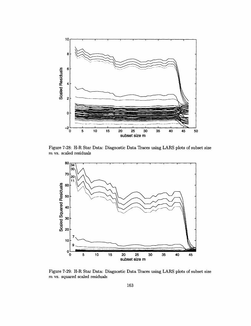
0 5 10 15 20 25 30 35 40 45 50subset size m
Figure 7-28: H-R Starm vs. scaled residuals
80
70
-- 60
.3
a0) 50
'a,- 40
30Cu
03 20
10
0
Data: Diagnostic Data Traces using LARS plots of subset size
0 5 10 15 20 25
subset size m30 35 40 45
Figure 7-29: H-R Star Data: Diagnostic Data Traces using LARS plots of subset sizem vs. squared scaled residuals
163
10
ua
'aU30
a,-0
8
6
4
2
0
-2
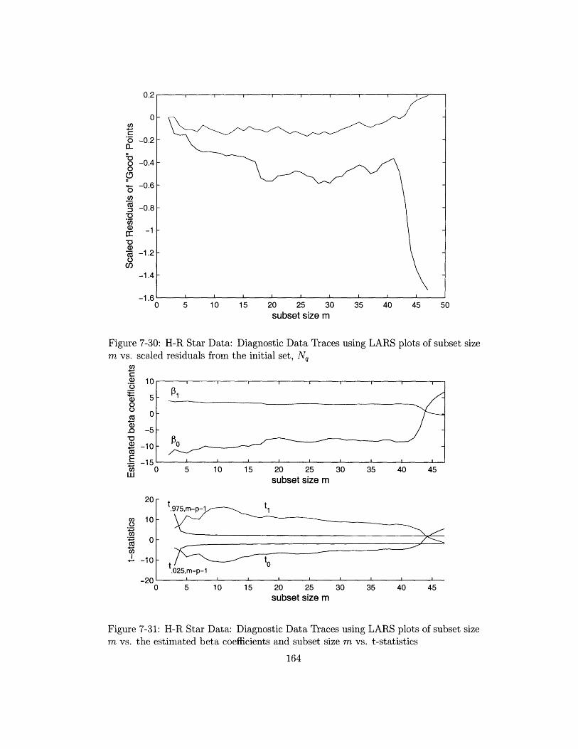
0.2
0
-0.2
-0.4
-0.6
-0.8
-1
-1.2
-1.4
-1 Ri
C 5 10 15 20 25 30
subset size m
Figure 7-30: H-R Star Data: Diagnostic Data Tracesm vs. scaled residuals from the initial set, Nq
-1
-1
10
0
-10
0
35 40 45 50
using LARS plots of subset size
5 10 15 20 25 30 35 40 45subset size m
J/1
.025,m-p-1i i l i i I I i i
0 5 10 15 20 25subset size m
30 35 40 45
Figure 7-31: H-R Star Data: Diagnostic Data Traces using LARS plots of subset sizem vs. the estimated beta coefficients and subset size m vs. t-statistics
164
,
oC
0o(D
a0C-
CZ
0CQ)O
Oa)0
'O.EaiCZEU,w
C,
C.,
CZI,
-2C
I I I I I 1 I I I
t.975,m-p1-~ t
I I I I I
I
1
^^ZU
I
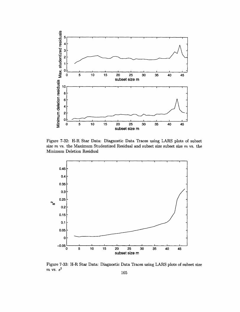
5 10 15 20 25subset size m
5 10 15 20 25subset size m
30 35 40 45
30 35 40 45
Figure 7-32: H-R Star Data: Diagnostic Data Traces using LARS plots of subsetsize m vs. the Maximum Studentized Residual and subset size subset size m vs. theMinimum Deletion Residual
0.45
0.4
0.35
0.3
0.25
0.2
0.15
0.1
0.05
0
0-v.v.,
0 5 10 15 20 25 30 35 40 45
subset size m
Figure 7-33:m vs. 2
H-R Star Data: Diagnostic Data Traces using LARS plots of subset size
165
0
V)
': 5
a 3N- 2
a,I 1
x 0
E 2._E 0
LE
CMon
· ·
· · · ·
· · · · · · ·
I_
a
n n:-- I I I I~ I I I I I I I I I
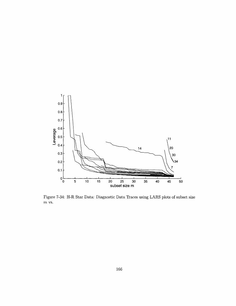
0.
0.
0.
a) 0.0)' 0.
0.
0.
0.0.
0 5 10 15 20 25 30 35 40 45 50
subset size m
Figure 7-34: H-R Star Data: Diagnostic Data Traces using LARS plots of subset sizem vs.
166
I1

Appendix
Data Sets
167
A
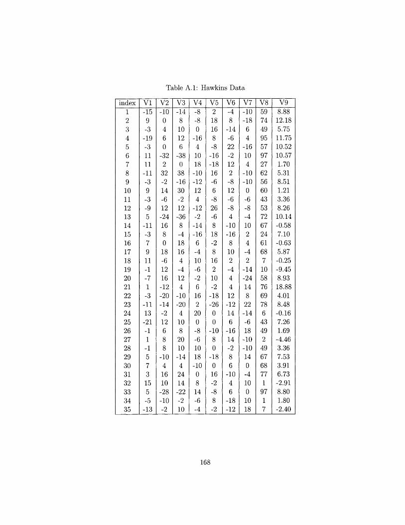
Table A.1: Hawkins Data
V2-100
4
6
0
-322
32-2
14-612
-2416
8
0
18
-612
16
-12-20-14-2
12
6
8
8
-104
16
10
-28-10-2
V3-148
10
12
6
-380
38-1630-212
-368
-418
16
4
-412
4
-10-204
10
8
2010
-144
2414
-22-210
V4-8-80
-164
10
18
-10-1212
4-12-2-14-166
-410
-6-26
16
2
200
-8-610
18
-100
8
14
-6-4
V52
18
16
8
-8-16-1816
-66
-826-68
18
-28
16
2
10
-2-18-26
0
0
-108
0
-180
16
-2-88
-2
V6-48
-14-622-212
2
-812
-6-84
-10-16
8
10
2
-444
12
-1214
6
-1614
-28
6
-1046
-18-12
V7-10-18
6
4
-1610
4
-10-10
0
-6-8-410
2
4-42
-14-2414
8
22-14-618
-10-1014
0
-410
0
10
18
168
index1
2
3
45
6
7
8
9
10
11
12
13
14
15
16
1718
19
2021
22232425262728293031
32333435
V1-15
9
-3
-19-3
11
11
-11-39
-3
-95
-11-3
7
9
11
-1
-71
-3
-1113
-21-1
1
-1
5
7
3
15
5
-5
-13
V859744995579727625660435372
672461
687
10
5876
69786
43492
496768771
971
7
V98.88
12.185.75
11.7510.5210.571.705.318.511.213.368.26
10.14-0.587.10
-0.635.87
-0.25-9.458.9318.884.018.48-0.167.261.69
-4.463.367.533.916.73-2.918.801.80
-2.40_- .- . .- --- _. ----
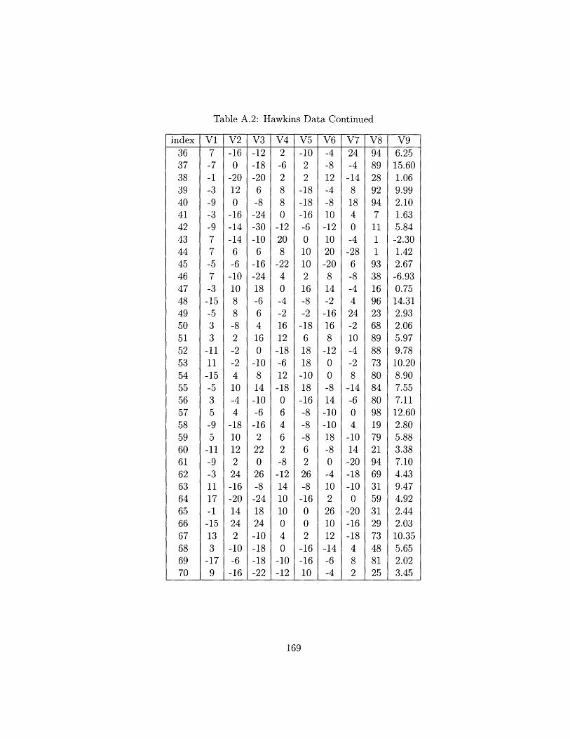
Table A.2: Hawkins Data Continued
V17-7-1
-3-9-3-9
77-57-3-15-53
3
-1111
-15-53
5-95
-11-9
-311
17-1
-1513
3
-179
V2-160
-2012
0
-16-14-146
-6-101088
-8
-2-2410
-44
-1810122
24-16-2014
242
-10-6
-16
V3-12-18-20
6
-8-24-30-10
6
-16-2418
-66
416
0
-108
14
-10-6
-162
220
26-8
-2418
24-10-18-18-22
V42
-62
8
8
0
-12208
-2240
-4-216
12
-18-6
12
-180
6
46
2
-8-1214
10
10
0
4
0
-10-12
V5-102
2
-18-18-16-6
01010
216
-8
-2
-186
18
18
-1018
-16-8-8
-8
6
2
26-8-160
0
2
-16-1610
V6-4-812
-4-810
-1210
20-20
8
14
-2-1616
8
-120
0
-814
-10-1018
-80
-410
2
2610
12
-14-6-4
V724-4
-148
18
40
-4-28
6
-8
-44
24-2
10
-4-2
8
-14-60
4-1014
-20-18-10
0
-20-16-1848
2
V894892892947
11
1
1
933816
962368898873
8084809819
79
21
946931
5931
29
73
4881
25
169
index363738394041
42434445464748495051
52535455565758596061
626364656667686970
V96.25
15.601.069.992.101.635.84
-2.301.422.67
-6.930.75
14.312.932.065.979.78
10.208.907.557.1112.602.805.883.387.104.439.474.922.442.03
10.355.652.023.45
---- --- .- --- .- --- .- .- ----
2
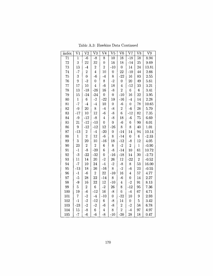
Table A.3: Hawkins Data Continued
vi
1
313
-73917
13
15
1
-7
-9-17-921
9-13
1
323-1
-311
-7-13
-1
-5-9519
7-1
-2315
-7
V2
-622-42
0
-210-18-24
6
-42010-12-12-12
2
2
202
-8-22141018
-6
28162
-6-2
-2-2-8-6
V3
-83224-6
0
4-26-24-2
-48
12
-8-10-12-412
10
2
-20-322024262
22226
-12-4-12-26
-6
V4
8
0
2
10
-48
-616
0
-2210-4-640
12-20-6
-166
6
0
-2-4
-1622-1412
-216
-106
-64-8
V510
16-100
8-2
18
-80
10
0
-8
-8-80
-260
8188-8
-1626-28
-108
-1026-80
-8-88
-10
V616
18
0
22-220
42
-10-16-62
6
18
-68
-14-14-12-2
-14-1812
-8-216
-6486
-2214
22
-20
V7-18
-1414
-10
16
20-12
6
16
-40
-6-12
-66
8
140
-82
1014
-228
-64
0
-2-12-4100
-2-428
[V8582524448349336
2214
782882759040946
12
1
61302
5323571491
95679
5
589718
170
index7172737475767778798081
828384858687888990919293949596979899100101102103104105
V98.949.6913.812.662.555.613.213.413.952.28
10.655.707.356.696.011.01
10.14-2.334.05-0.9010.72-2.72-0.5216.00-0.554.772.278.137.364.712.933.426.784.970.47
| Index
.----- . _ --- --- ----
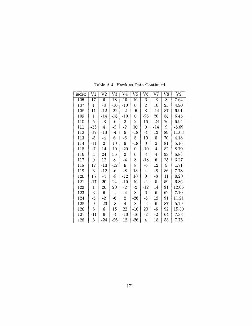
Table A.4: Hawkins Data Continued
index V26-8-12-14-84
-10-42142412-10-12-420206
-2-2066
-24
7.644.906.916.466.94
-8.6911.034.185.168.706.833.271.717.780.206.8612.067.1011.215.7915.307.337.76
171
11
1
5
-13-17-5
-11-7-59
173
15
-171
3
-59
5
-11
3
171
18
-10-22-18-6-2-46
10
10
368
-12-6-824202
-6-816
-4-26
10
-10-2
-102
-26
-66
-202
-46
-8-12-10-2-42
422-1012
VI V3 V4 V5 V6 V7 V8 V9106107108109110ill112113114115116117118119120121122123124125126127128
16
0
-60
2
10
-188
-180
6
8
8
18
1016
-28
-268
-10-16-26
6
2
8
-2616
0
-4100
-10-4
-18-64
0
-2-12
6
-8-220-24
-810
-1420-24-1412
02
446
12
-8-8014
6
12
6
-6-2is
8
238758769
8970818298259
8611
59916291
87926453
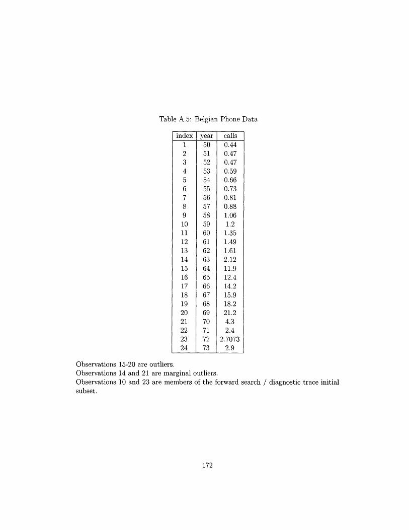
Table A.5: Belgian Phone Data
Observations 15-20 are outliers.Observations 14 and 21 are marginal outliers.Observations 10 and 23 are members of the forward search / diagnostic trace initialsubset.
172
index0.440.470.470.590.660.730.810.881.061.2
1.351.491.612.1211.912.414.215.918.221.24.32.4
2.70732.9
year calls1
2
3
45
6
7
8
9
1011
12
13
1415
16
171819
2021222324
5051
52535455565758596061
62636465666768697071
7273
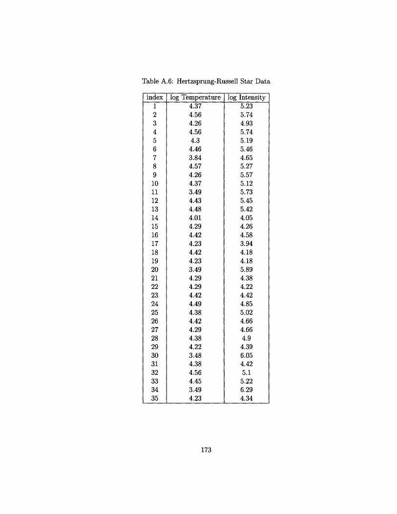
Table A.6: Hertzsprung-Russell Star Data
log Temperature4.374.564.264.564.3
4.463.844.574.264.373.494.434.484.014.294.424.234.424.233.494.294.294.424.494.384.424.294.384.223.484.384.564.453.494.23
log Intensity5.235.744.935.745.195.464.655.275.575.125.735.455.424.054.264.583.944.184.185.894.384.224.424.855.024.664.664.9
4.396.054.425.1
5.226.294.34
173
index1
23456
7891011
12
13141516
171819202122232425262728293031
32333435
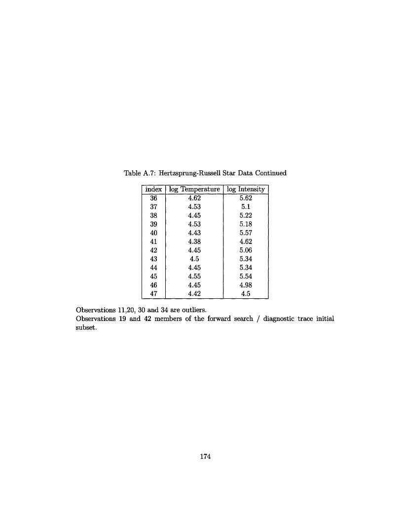
Table A.7: Hertzsprung-Russell Star Data Continued
index log Temperature log Intensity36 4.62 5.6237 4.53 5.138 4.45 5.2239 4.53 5.1840 4.43 5.5741 4.38 4.6242 4.45 5.0643 4.5 5.3444 4.45 5.3445 4.55 5.5446 4.45 4.9847 4.42 4.5
Observations 11,20, 30 and 34 are outliers.Observations 19 and 42 members of the forward search / diagnostic trace initialsubset.
174

Appendix B
Tables
Table B.1: Results of simulations to the test the dLARS orderings as in Khan et. al.[34]
175
Uniform Leverageel e2 e3 e4 el e2 e3 e4
LARS- Exact (E) 97 86 11 8 0 1 1 2LARS- Global (G) 100 89 26 24 0 2 5 7
dLARS Simple: T order, (E) 95 95 61 83 96 95 65 85dLARS Simple: T order, (G) 100 100 80 88 100 99 85 91
dLARS Simple: LARS order, (E) 89 81 4 3 43 57 21 21dLARS Simple: LARS order, (G) 100 96 14 14 99 97 36 44
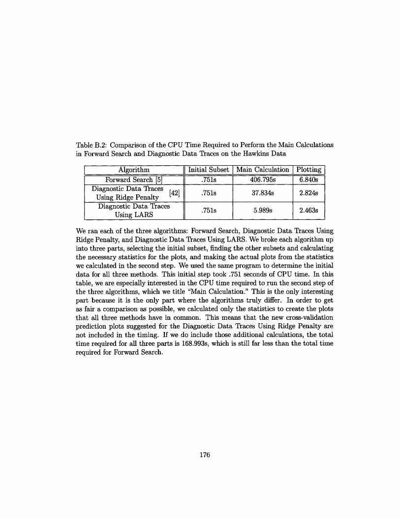
Table B.2: Comparison of the CPU Time Required to Perform the Main Calculationsin Forward Search and Diagnostic Data Traces on the Hawkins Data
We ran each of the three algorithms: Forward Search, Diagnostic Data Traces UsingRidge Penalty, and Diagnostic Data Traces Using LARS. We broke each algorithm upinto three parts, selecting the initial subset, finding the other subsets and calculatingthe necessary statistics for the plots, and making the actual plots from the statisticswe calculated in the second step. We used the same program to determine the initialdata for all three methods. This initial step took .751 seconds of CPU time. In thistable, we are especially interested in the CPU time required to run the second step ofthe three algorithms, which we title "Main Calculation." This is the only interestingpart because it is the only part where the algorithms truly differ. In order to getas fair a comparison as possible, we calculated only the statistics to create the plotsthat all three methods have in common. This means that the new cross-validationprediction plots suggested for the Diagnostic Data Traces Using Ridge Penalty arenot included in the timing. If we do include those additional calculations, the totaltime required for all three parts is 168.993s, which is still far less than the total timerequired for Forward Search.
176
Algorithm Initial Subset Main Calculation PlottingForward Search [5] .751s 406.795s 6.840s
Diagnostic Data Traces 37.834s 2.824sUsing Ridge PenaltyDiagnostic Data Traces.751s 5.989s 2.463s
Using LARS
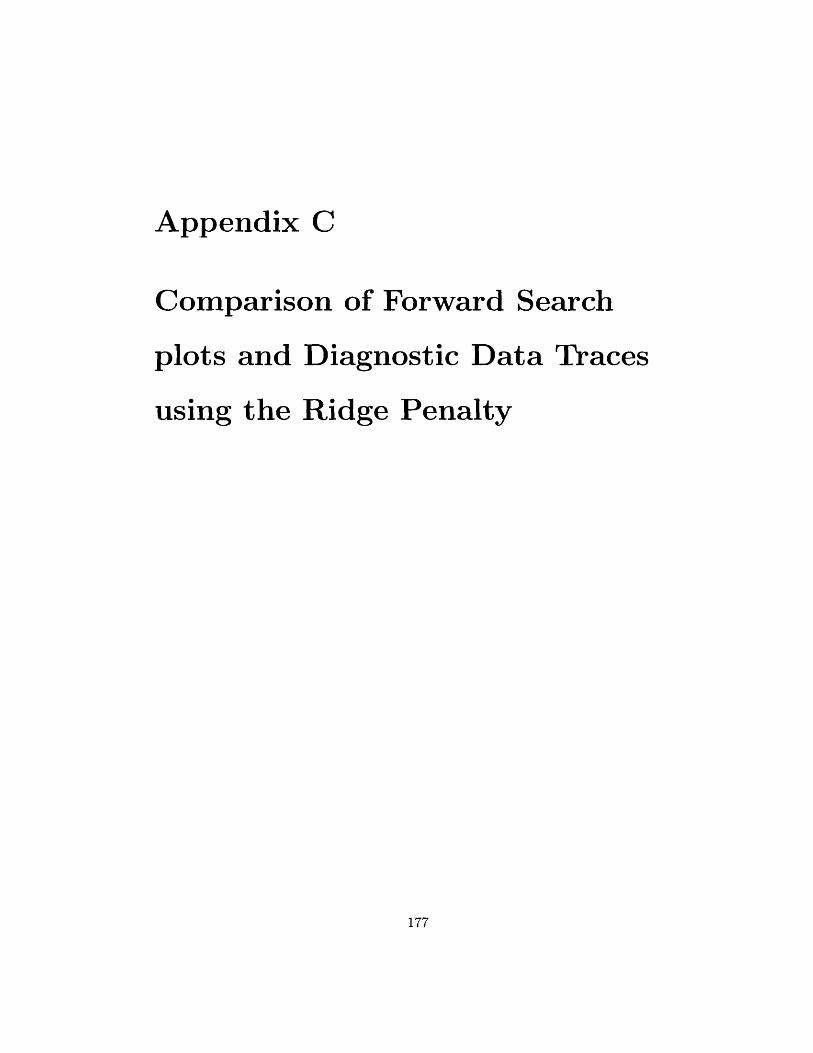
Appendix
Comparison of Forward Search
plots and Diagnostic Data Traces
using the Ridge Penalty
177
C
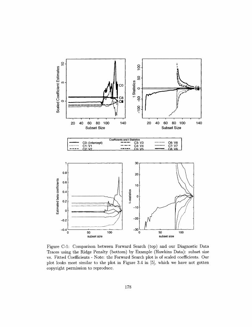
o0
C,U)ccEa)
._a)0oV
a)CO0
C/)
20 40 60 80 100Subset Size
140
U)
._o
C.
n
20 40 60 80 100Subset Size
140
Coefficients and t StatisticsCO: (Intercept) 0.. C3:V3 0...... C6: V6
..... C1:V1 . . C4:V4 ........ C7:V70.C2:V2 C VS Ca VR
50 100subset size
Co0)lo
CoIn
0 50 100subset size
Figure C-1: Comparison between Forward Search (top) and our Diagnostic DataTraces using the Ridge Penalty (bottom) by Example (Hawkins Data): subset sizevs. Fitted Coefficients - Note: the Forward Search plot is of scaled coefficients. Ourplot looks most similar to the plot in Figure 3.4 in [5], which we have not gottencopyright permission to reproduce.
178
0.8
0.6
0.4
0.2
Co
'E
.9
C0
.)00Cc
0.0
ELIwU
-0.2
-0.40
_ ·
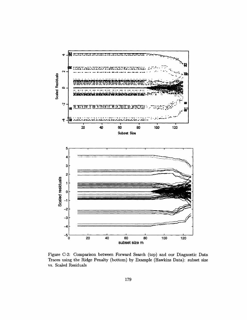
:043
GPIX a
..-] _ :_-.-._ -..-- .-.-:---,.,-.:. ._,--;, ------. _---:: .-.: .'R
!I-=I~ "~·J~-"·I"~. "- - - -- n * . : : . ' : * ' -: '' - 'L A- : s-: 'V : '.":: .. -:--:
20 40 60 80 100 120
Subset Size
5
4 u,~~~~~~~~~~~~~[. ... .....
1.u'Ja
-2
-3
-4
-55 I I I .0 20 40 60 80 100 120subset size m
Figure C-2: Comparison between Forward Search (top) and our Diagnostic DataTraces using the Ridge Penalty (bottom) by Example (Hawkins Data): subset sizevs. Scaled Residuals
179
. .. . . . ... .............. ...... ................... .- .
_._lql ~- _,- _,,q. q.mll.H..-m ".-- -· .-it- [ - -e- ·- - ·,, ''- .'. '' .,i"
_ _ _ _-- ------ ~- W21 _
, ,· ' W W r_4 _ *,, --- ,-* m :_- ,- - *.--.-- .. '
s 1 . . _ . _ . . . .·· Z. ... _..WQ -· --- - -_ __ __
i
I
o-
20 40 60 80 100 120
Subset Size
0 20 40 60 80 100 120subset size
Figure C-3: Comparison between Forward Search (top) and our Diagnostic DataTraces using the Ridge Penalty (bottom) by Example (Hawkins Data): subset sizevs. Scaled Squared Residuals
180
U,
U)
-ocu0a,
"r
CO(/3
o0
LO-
19s--------------------------------191, 1 - - .......... .......... .............
.... ..=. ...... .....
................... ................. . .............................. ... .'1, '' r' l lrel' Iwe'm ' ',r l' u l ' l i l f T , lnf nrd'v l 1relr n d t,' r1 '. o. '-- ._ .. ,.. · ' ...?' . '..
.r _8S
.. m- _. I, ~~~~~~~\\5, %.,s
....................... ................... ................... ··· ·.. .= ago|@~~~~~~~~~~~~~~~~~~~~::~ !,,,___ | _~~~~~~~~~~~~~~~~~~~~..:.'.'..
-!a1
a:
C
CrC.c
(aCDCo
I I I I
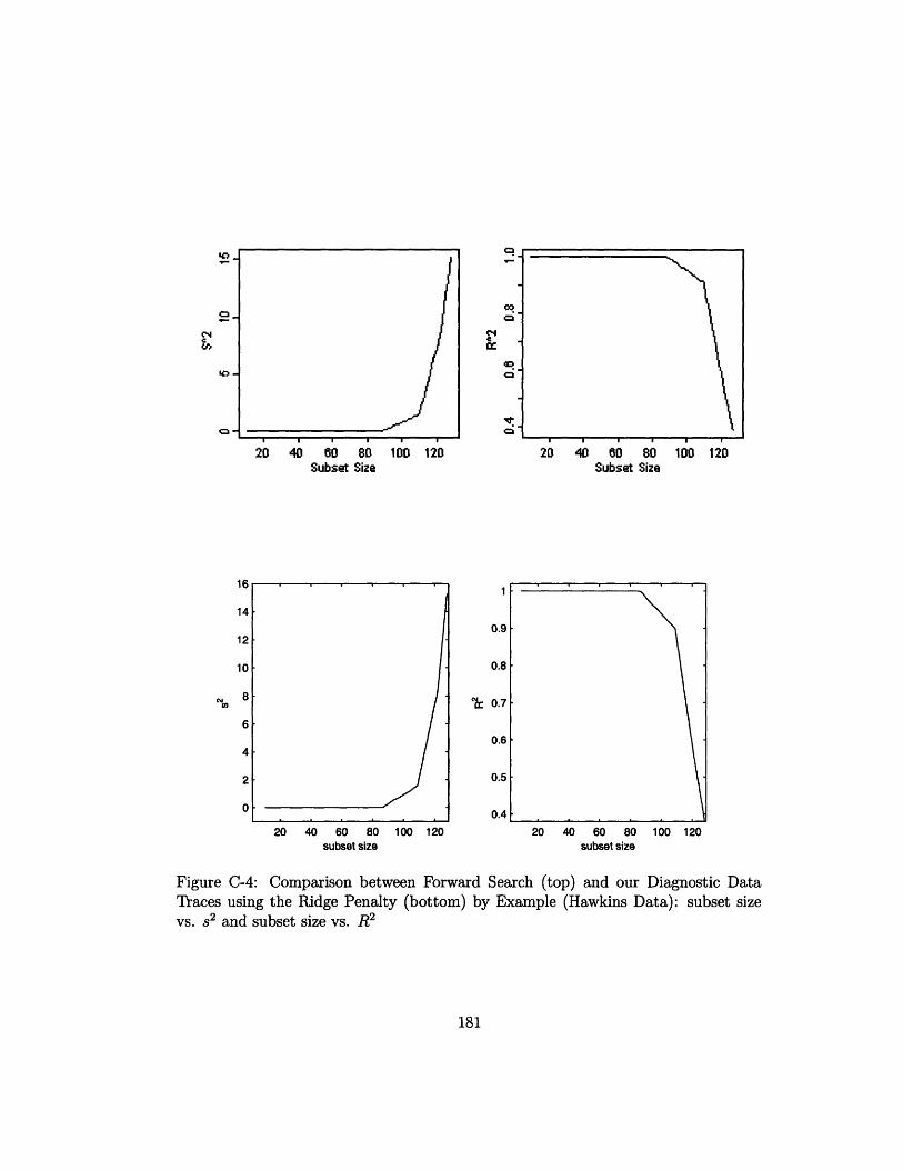
20 40 60 80Subset Size
c:>
Ca0
NcI
c
100 120 20 40 60 80Subset Size
0.9
0.8
0.6
0.5
0.4
100 120
20 40 60 80 100 120 20 40 60 80 100 120subset size subset size
Figure C-4: Comparison between Forward Search (top) and our Diagnostic DataTraces using the Ridge Penalty (bottom) by Example (Hawkins Data): subset sizevs. s2 and subset size vs. R 2
181
c4Ch
c-
(a
_ _
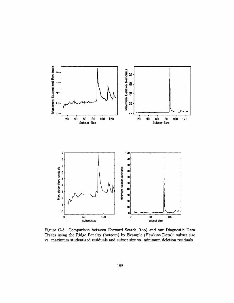
20 40 60 80Subset Size
m'A
w.0 Ca
a cDrc0Ix C3
.0
E_0cm
.9 C
loo 120 20 40 60 80Subset Size
IUU
90
80
E 60C0Z 50
E 40
E 30
20
10
00 50 100
subset size50subset size
100 120
100
Figure C-5: Comparison between Forward Search (top) and our Diagnostic DataTraces using the Ridge Penalty (bottom) by Example (Hawkins Data): subset sizevs. maximum studentized residuals and subset size vs. minimum deletion residuals
182
rwa'
EE
m= C.
0f)
' a#CU*0-0V
.
11-.
I
A- --,I _-
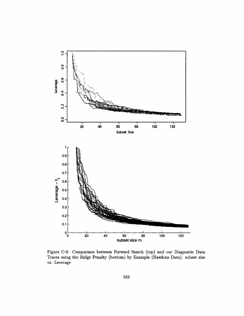
20 40 60 80 100 120
Subset Size
20 40 60 80
subset size m100 120
Figure C-6:Traces usingvs. Leverage
Comparison between Forward Search (top) and our Diagnostic Datathe Ridge Penalty (bottom) by Example (Hawkins Data): subset size
183
·-
Co
en
_
1
0.9
0.8
0.7
0.6.-=
(Dc~l)_n
0.5
0.4
0.3
0.2
0.1
0II I I !

184

Appendix
Complete Set of Diagnostic
Traces using the Ridge Penalty for
the Belgian Phone
185
Data
Data
D
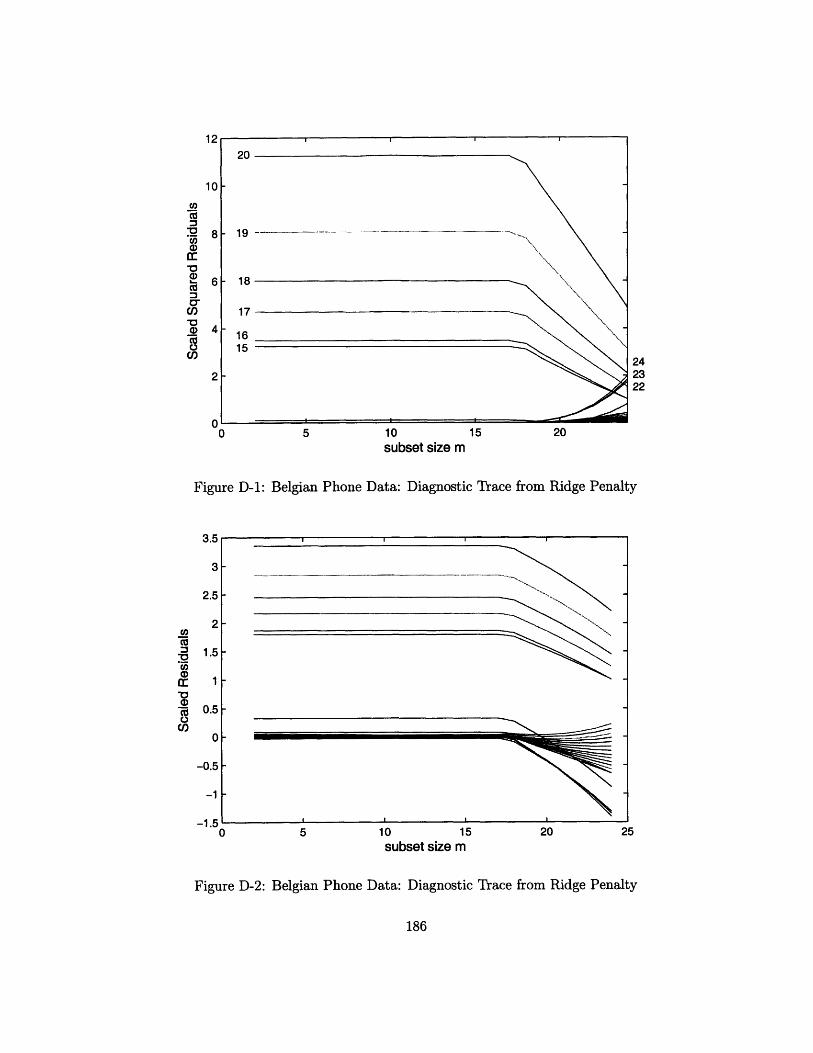
242322
0 5 10 15 20subset size m
Figure D-1: Belgian Phone Data: Diagnostic Trace from Ridge Penalty
3
2.5
2
1.5
1
0.5
0
-0.5
-1
0 5 10 15 20 25subset size m
Figure D-2: Belgian Phone Data: Diagnostic Trace from Ridge Penalty
186
*0
a)(O
Ca
0*Cl
C)
-o!)
/)
Ei 1
--1
1
-. A<
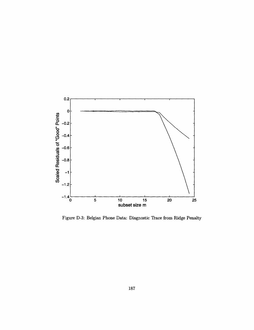
o
oun -0.2o -0.4(50
u -0.6cu' -0.80') -- 1
CIS
-1.2
_1 A
0 5 10 15 20 25subset size m
Figure D-3: Belgian Phone Data: Diagnostic Trace from Ridge Penalty
187
1
I0.2
A -
- I - - - -- - I -
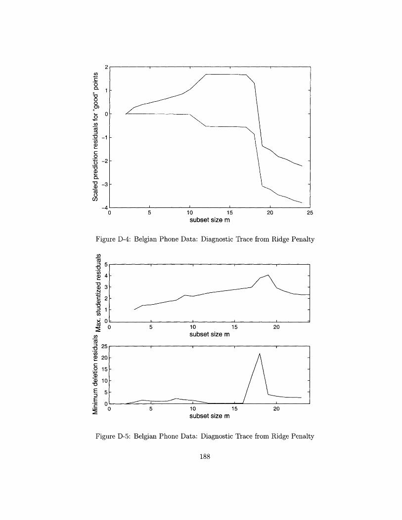
5 10 15 20 25
subset size m
Figure D-4: Belgian Phone Data: Diagnostic Trace from Ridge Penalty
C,c7
5 10
subset size m15 20
5 10 15 20
subset size m
Figure D-5: Belgian Phone Data: Diagnostic Trace from Ridge Penalty
188
2U,C-Oe.
000)oo,0o
C._V/)
0ta0C')
1
0
-1
-2
-3
-40
_rU)(D 4
03N
C 2
1'ix0(
CO
01
a 20
.2 15a)a3 10
E 5
E C C
· · · ·
· · I I
· · · ·
· · · ·
)o
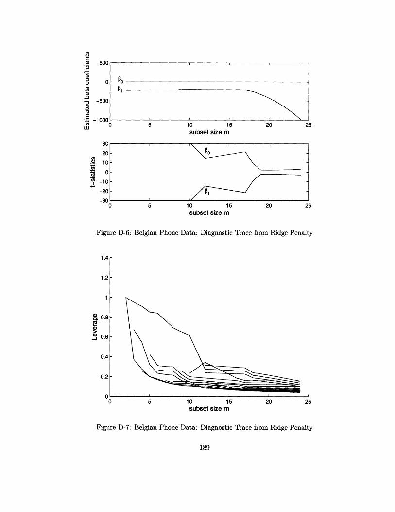
500
0
-500
-1000
30
20
10
0
-10
-20
- 0
01
0 5 10 15 20 2;
subset size m
0 5 10 15 20
5
25subset size m
Figure D-6: Belgian Phone Data: Diagnostic Trace from Ridge Penalty
1.4
1.2
1
0.8
0.6
0.4
0.2
00 5 10 15 20
subset size m25
Figure D-7: Belgian Phone Data: Diagnostic Trace from Ridge Penalty
189
a)
._)
CD0C,.011Ec'w
8C',
Cuw'
I\ .o,
, 13 . ,
a)0)
a)a)-j
I
I-an L
J r
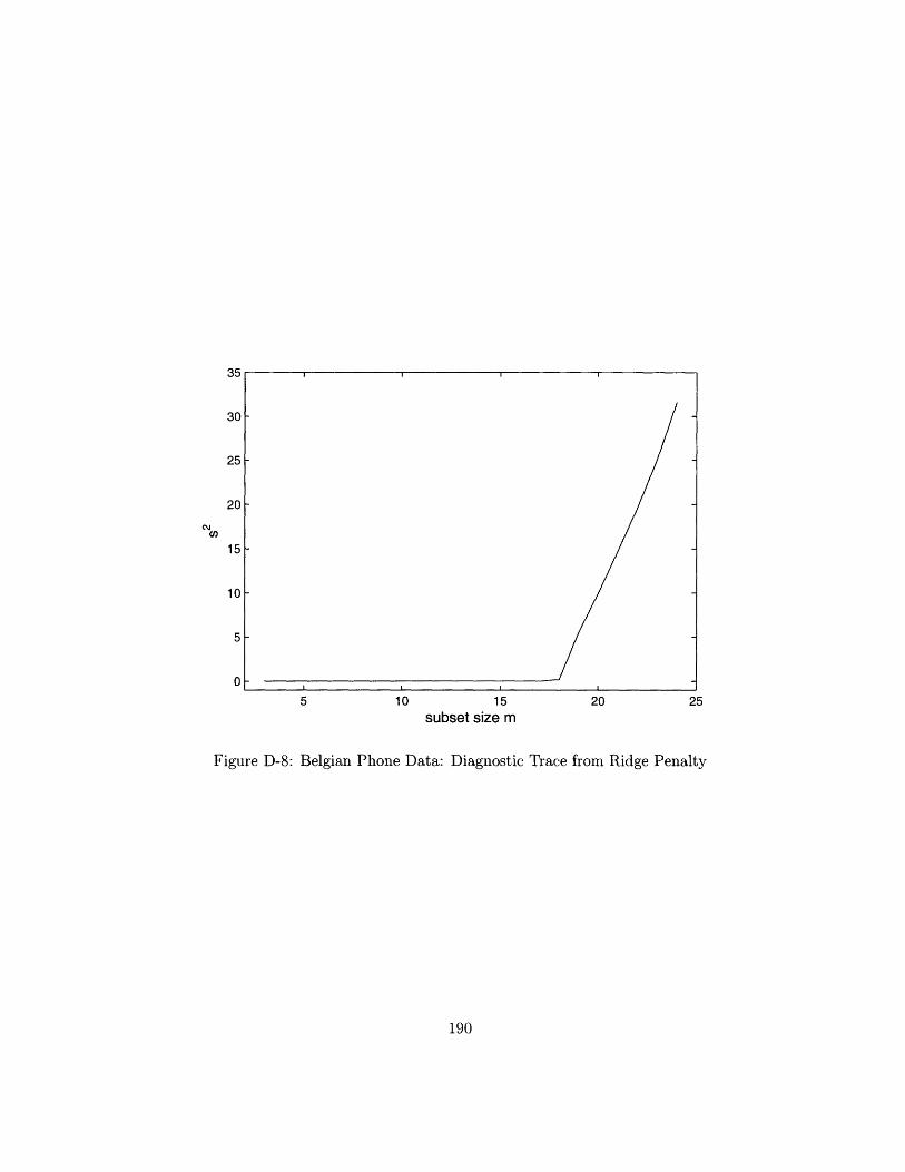
OI
30
25
20
C/)
15
10
5
nI I I 2
5 10 15 20 25
subset size m
Figure D-8: Belgian Phone Data: Diagnostic Trace from Ridge Penalty
190
-- -T- I - -r - --
v

Bibliography
[1] Claudio Agostinelli. Robust model selection in regerssion via weighted likelihood
methodology. Statistics and Probability Letters, 56:289-300, 2002.
[2] H. Akaike. Statistical predictor identification. Ann. Inst. Statist. Math., 22:203-
217, 1970.
[3] H. Akaike. Information theory and an extension of the maximum likelihood
principle. In B. N. Petrov and F. CsAiki, editors, 2nd International Symposium
on Information Theory, pages 267-281. Budapest: Akad6mia Kiado, 1973.
[4] H. Akaike. A new look at the statistical model identification. I.E.E.E. Trans.
Auto. Control, 19:716-723, 1974.
[5] Anthony Aktinson and Marco Riani. Robust Diagnistic Regression Analysis.
Springer-Verlag, first edition, 2000.
[6] D. M. Allen. The relationship between variable selection and prediction. Tech-
nometrics, 16:125-127, 1974.
[7] A. C. Atkinson. Masking unmasked. Biometrika, 73(3):533-541, 1986.
[8] David A. Belsley, Edwin Kuh, and Roy E. Welsch. Regression Diagnostics. Wiley,
1980.
[9] Richard Berk. An introduction to ensemble methods for data analysis. Technical
Report 2004072501, UCLA Department of Statistics, July 2004.
191
[10] Leo Breiman. Better subset regression using the nonnegative garrote. Techno-
metrics, 37(4):373-383, 1995.
[11] Leo Breiman. Bagging predictors. Machine Learning, 24(2):123-140, 1996.
[12] George Casella and Roger L. Berger. Statistical Inference. Duxbury, second
edition, 2001.
[13] Samprit Chatterjee and Ali S. Hadi. Influential observations, high leverage
points, and outliers in regression. Statistical Science, 1(3):379-416, 1986.
[14] Bradley Efron, Trevor Hastie, Iain Johnstone, and Robert Tibshirani. Least
angle regression. The Annals of Statistics, 32(2):407-499, 2004.
[15] M. Efroymson. Mathematical Methods for Digital Computers, chapter Multiple
regression analysis. Wiley, 1960.
[16] I. E. Frank and J. H. Friedman. A statistical view of some chemometrics tools.
Technometrics, 35:109-148, 1993.
[17] Ildiko E. Frank and Jerome H. Friedman. A statistical view of some chemometrics
regression tools. Technometrics, 35(2):109-148, 1993.
[18] Wing-Kam Fung. Unmasking outliers and leverage points: A confirmation. Jour-
nal of the American Statistical Association, 88(422):515-519, 1993.
[19] E. I. George and R. E. McCulloch. Variable selection via gibbs sampling. Journal
of the American Statistical Association, 88:881-889, 1993.
[20] William Guthrie, James Filliben, and Alan Heckert. Nist/sematech e-handbook
of statistical methods.
[21] Ali S. Hadi. Identifying multiple outliers in multivariate data. Journal of Royal
Statistical Society, Series B, 54(3):761-771, 1992.
192
[22] Ali S. Hadi and Jeffrey S. Simonoff. Procedures for the identification multi-
ple outliers in linear models. Journal of the American Statistical Association,
88(424):1264-1272, 1993.
[23] Trevor Hastie, Jonathan Taylor, Robert Tibshirani, and Guether Walther. For-
ward stagewise regression and the monotone lasso. Technical report, Stanford
University, March 2006.
[24] Trevor Hastie, Robert Tibshirani, and Jerome Friedman. The Elements of Sta-
tistical Learning. Springer-Verlag, 2001.
[25] D. M. Hawkins, D. Bradu, and G. V. Kass. Location of several outliers in
multiple-regression data using elemental sets. Technometrics, 26:197-208, 1984.
[26] Douglas M. Hawkins. The accuracy of elemental set approximations for regres-
sion. Journal of the American Statistical Association, 88(422):580-589, 1993.
[27] U. Hjorth. On model selection in the computer age. Journal of Statistical Plan-
ning and Inference, 23:101-115, 1989.
[28] Arthur E. Hoerl and Robert W. Kennard. Ridge regression: Applications to
nonorthogonal problems. Technometrics, 12(1):68-82, 1970.
[29] Arthur E. Hoerl and Robert W. Kennard. Ridge regression: Biased estimation
for nonorthogonal problems. Technometrics, 12(1):55-67, 1970.
[30] Jennifer Hoeting, Adrian E. Raftery, and David Madigan. A method for simul-
taneous variable selection and outlier identification in linear regression. Compu-
tational Statistics and Data Analysis, 22:251-270, 1996.
[31] P. J. Huber. Robust regression: Asymptotics, conjectures, and monte carlo.
Annals of Statistics, 1:799-821, 1973.
[32] Peter J. Huber. Robust Statistics. John Wiley and Sons.
[33] Joseph B. Kadane and Nicole A. Lazar. Methods and criteria for model selection.
Journal of the American Statistical Association, 99(465):279-, March 2004.
193
[34] Jafar A. Khan, Stefan Van Aelst, and Ruben H. Zamar. Robust linear model
selection based on least angle regression. September 13, 2005.
[35] Keith Knight. Discussion: Least angle regression. The Annals of Statistics,
32(2):458-460, 2004.
[36] W. S. Krasker and R. E. Welsch. Efficient bounded influence regression estima-
tion. Journal of the American Statistical Association, 77:596-604, 1982.
[37] L. Kuo and B. Mallick. Variable selection for regression models. Sankhya, 60:65-
81, 1998.
[38] Kenneth Lange. Numerical Analysis for Statisticians. Springer, 1999.
[39] Ker-Chau Li. Asymptotic optimality for Cp, cL, cross-validation and generalized
cross-validation: Discrete index set. The Annals of Statistics, 15(3):958-975,
1987.
[40] C. L. Mallows. Some comments on cp. Technometrics, 15:661-675, 1973.
[41] C. L. Mallows. More comments on cp. Technometrics, 37:362-372, 1995.
[42] Lauren McCann and Roy E. Welsch. Diagnostic data traces using penalty meth-
ods. In Proceedings of in Computational Statistics, 2004.
[43] Alan Miller. Subset Selection in Regression. Chapman and Hall, second edition,
2002.
[44] T. J. Mitchell and J. J. Beauchamp. Bayesian variable selection in linear regres-
sion. Journal of the American Statistical Association, 83:1023-1036, 1988.
[45] Stephan Morgenthaler, Roy E. Welsch, and Andrei Zenide. Algorithms for robust
model selection. 2004.
[46] A. E. Raftery, D. Madigan, and J. A. Hoeting. Bayesian model averaging for
linear regression models. Journal of the American Statistical Association, 92:179-
191, 1997.
194

[47] William J. J. Rey. Introduction to Robust and Quasi-Robust Statistical Methods.
Springer-Verlag, 1983.
[48] E. Ronchetti. Robust model selection in regression. Statistics and Probability
Letters, 3:21-23, 1985.
[49] E. Ronchetti and R. G. Staudte. A robust version of mallows' cp. Journal of the
American Statistical Association, 89:550-559, 1994.
[50] Elvezio Ronchetti, Christoper Field, and Wade Blanchard. Robust linear model
selection by cross-validation. Journal of the American Statistical Association,
92(439):1017-1023, September 1997.
[51] P. J. Rousseeuw and A. M. Leroy. Robust Regression and Outlier Detection. John
Wiley, 1987.
[52] P. J. Rousseeuw and B. van Zomeren. Unmasking multivariate outliers and
leverage points. Journal of the American Statistical Association, 85:633-639,
1990.
[53] P. J. Rousseeuw and V. J. Yohai. Robust and Nonlinear Time Series, chap-
ter Robust regression by means of S-estimators, pages 256-272. Number 26 in
Lecture Notes in Statistics. Springer, 1984.
[54] Peter J. Rousseeuw. Least median of squares regression. Journal of the American
Statistical Association, 79:871-880, 1984.
[55] Peter J. Rousseeuw and Christophe Croux. Alternatives to the median absolute
deviation. Journal of the American Statistical Association, 88(424):1273-1283,
December 1993.
[56] Willi Sauerbrei. The use of resampling methods to simplify regression models in
medical statistics. Applied Statistics, 48(3):313-329, 1999.
[57] Jun Shao. Linear model selection by cross-validation. Journal of the American
Statistical Association, 88(422):486-494, June 1993.
195
[58] Suzanne Sommer and Robert G. Staudte. Robust variable selection in regression
in the presence of outliers and leverage points. Australian Journal of Statistics,
37(3):323-336, 1995.
[59] N. Sugiura. Further analysis of the data by akaike's information criterion and
the finite corrections. Commun. Statist. A, 7:13-26, 1978.
[60] H. Theil and A.S. Goldberger. On pure and mixed estimation in economics.
International Economic Review, 2:65-78, 1961.
[61] R. Tibshirani. Regression shrinkage and selection via the lasso. Journal of the
Royal Statistical Society Series B, 61:529-546, 1996.
[62] J. Tukey. Contributions to Probability and Statistics, chapter A Survey of Sam-
pling From Contaminated Distributions. Standford University Press: Stanford,
California, 1960.
[63] S. Weisberg. Applied Linear Regression. Wiley, second edition, 1985.
[64] Ming Yuan and Yi Lin. Model selection and estimation in regression with grouped
variables. Technical Report 1095, University of Wisconsin Department of Statis-
tics, November 2004.
[65] Hui Zou and Trevor Hastie. Regularization and variable selection via the elastic
net. Journal of the Royal Statistical Society: Series B, 67(2):301-320, 2005.
196