Robust Methods in Computer Vision

CS 763

Ajit Rajwade

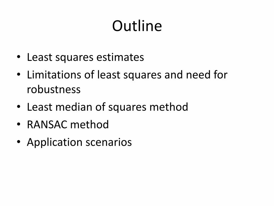
Outline

• Least squares estimates

• Limitations of least squares and need for robustness

• Least median of squares method

• RANSAC method

• Application scenarios

Least squares Estimates

• Consider quantity y related to quantity x in the form y = f(x;a).

• Here a is a vector of parameters for the function f. For example, y = mx + c, where a = (m,c).

• Now consider, we have N data points (xi,yi) where the yi could be possibly corrupted by noise, and want to estimate a.

• This is done by minimizing the following w. r. t. a:

N

i

ii xfy1

2));(( a

Least squares Estimates

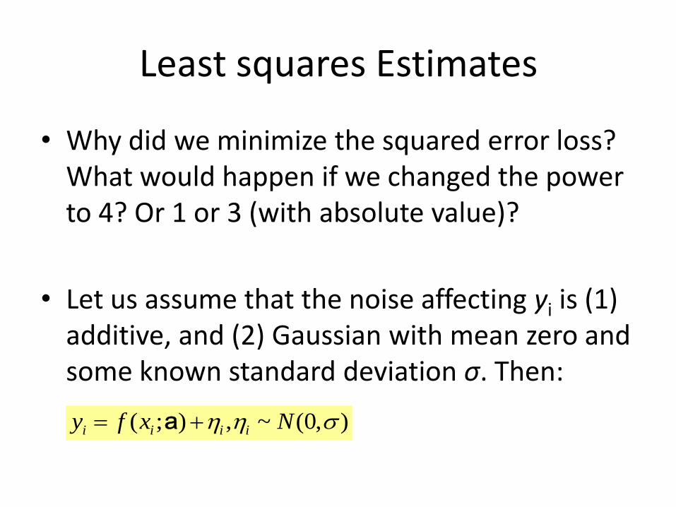
• Why did we minimize the squared error loss? What would happen if we changed the power to 4? Or 1 or 3 (with absolute value)?

• Let us assume that the noise affecting yi is (1) additive, and (2) Gaussian with mean zero and some known standard deviation σ. Then:

),0(~,);( Nxfy iiii a

Least squares Estimates

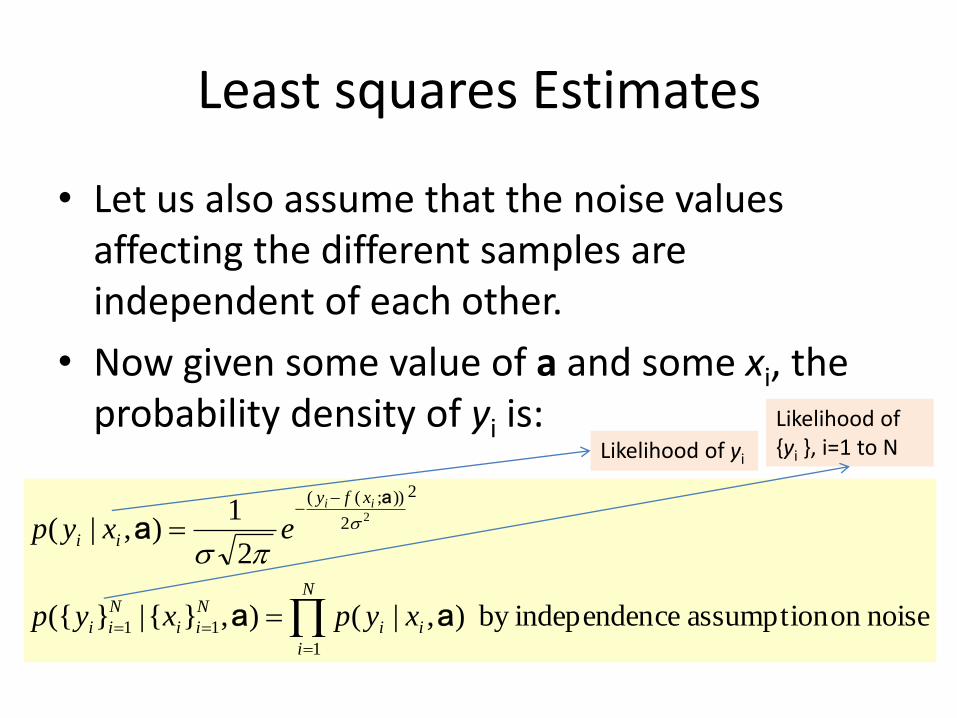
• Let us also assume that the noise values affecting the different samples are independent of each other.

• Now given some value of a and some xi, the probability density of yi is:

noise on assumption ceindependenby ),|(),}{|}({

2

1),|(

1

11

2

2

));((2

N

i

ii

N

ii

N

ii

xfy

ii

xypxyp

exypii

aa

a

a

Likelihood of yi

Likelihood of {yi }, i=1 to N

Least squares Estimates

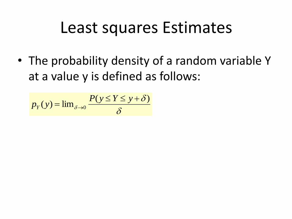
• The probability density of a random variable Y at a value y is defined as follows:

)(lim)( 0

yYyPypY

Least Squares Estimates

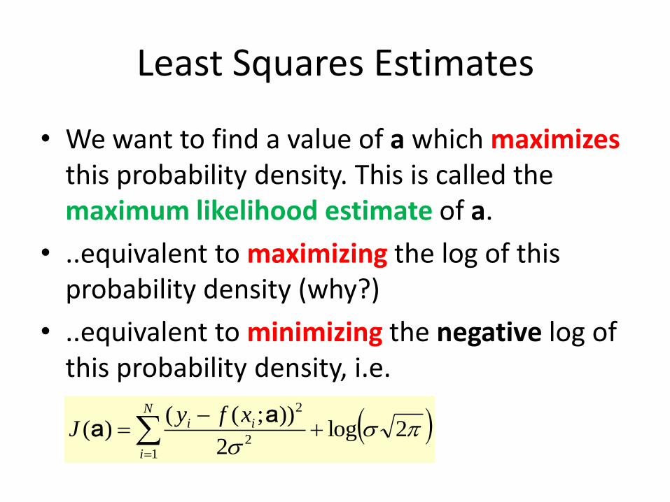
• We want to find a value of a which maximizesthis probability density. This is called the maximum likelihood estimate of a.

• ..equivalent to maximizing the log of this probability density (why?)

• ..equivalent to minimizing the negative log of this probability density, i.e.

2log2

));(()(

12

2

N

i

ii xfyJ

aa

Least Squares Estimates

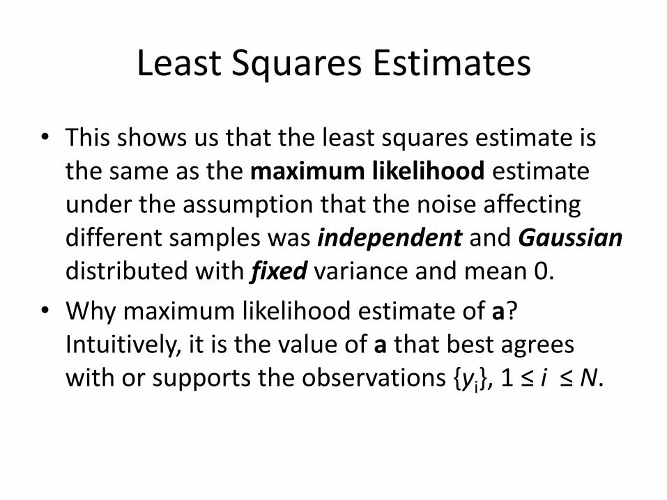
• This shows us that the least squares estimate is the same as the maximum likelihood estimate under the assumption that the noise affecting different samples was independent and Gaussiandistributed with fixed variance and mean 0.

• Why maximum likelihood estimate of a? Intuitively, it is the value of a that best agrees with or supports the observations {yi}, 1 ≤ i ≤ N.

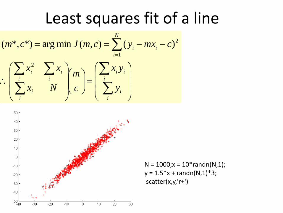
Least squares fit of a line

i

i

i

ii

i

i

i

i

i

i

N

i

ii

y

yx

c

m

Nx

xx

cmxycmJcm

2

1

2)(),(minarg*)*,(

N = 1000;x = 10*randn(N,1);y = 1.5*x + randn(N,1)*3;scatter(x,y,'r+')

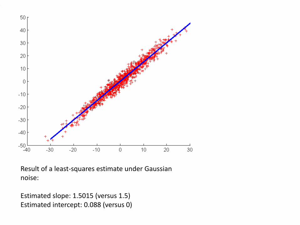
Result of a least-squares estimate under Gaussian noise:

Estimated slope: 1.5015 (versus 1.5)Estimated intercept: 0.088 (versus 0)

Other Least-squares solutions in computer vision

• Camera calibration – SVD

• Parametric motion estimation – SVD or pseudo-inverse (affine, rotation, homography, etc)

• Fundamental/essential matrix estimation –SVD (we will study this later in stereo-vision)

• Optical Flow (Horn-Shunck as well as Lucas-Kanade) (we will study this later)

Outliers and Least-squares estimates

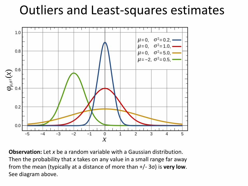
Observation: Let x be a random variable with a Gaussian distribution. Then the probability that x takes on any value in a small range far away from the mean (typically at a distance of more than +/- 3σ) is very low. See diagram above.

Outliers and Least-squares

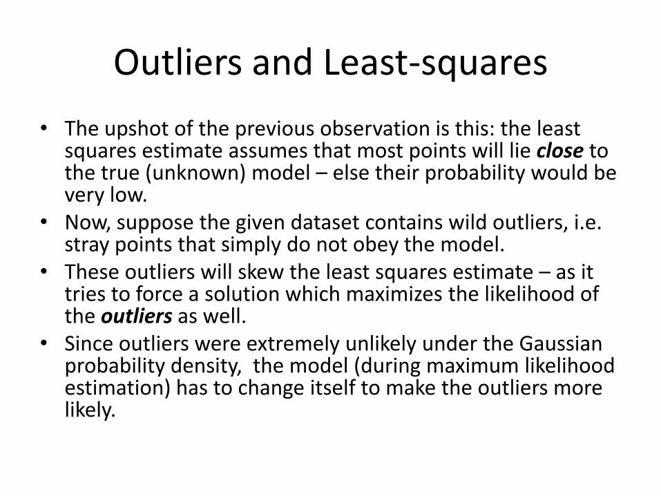
• The upshot of the previous observation is this: the least squares estimate assumes that most points will lie close to the true (unknown) model – else their probability would be very low.

• Now, suppose the given dataset contains wild outliers, i.e. stray points that simply do not obey the model.

• These outliers will skew the least squares estimate – as it tries to force a solution which maximizes the likelihood of the outliers as well.

• Since outliers were extremely unlikely under the Gaussian probability density, the model (during maximum likelihood estimation) has to change itself to make the outliers more likely.

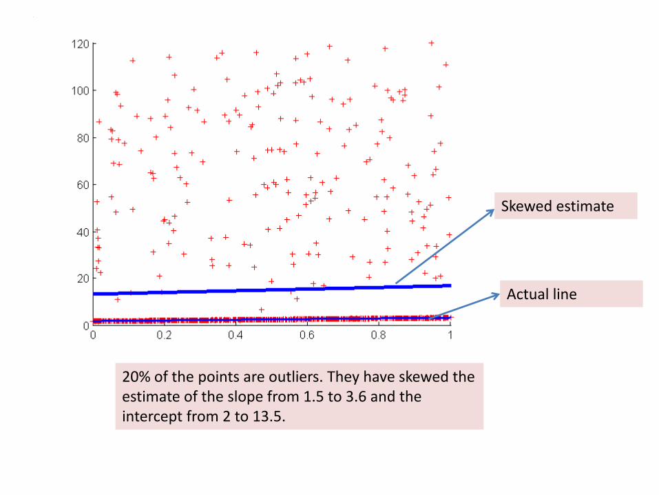
20% of the points are outliers. They have skewed the estimate of the slope from 1.5 to 3.6 and the intercept from 2 to 13.5.

Skewed estimate

Actual line

Examples of outliers: (1)

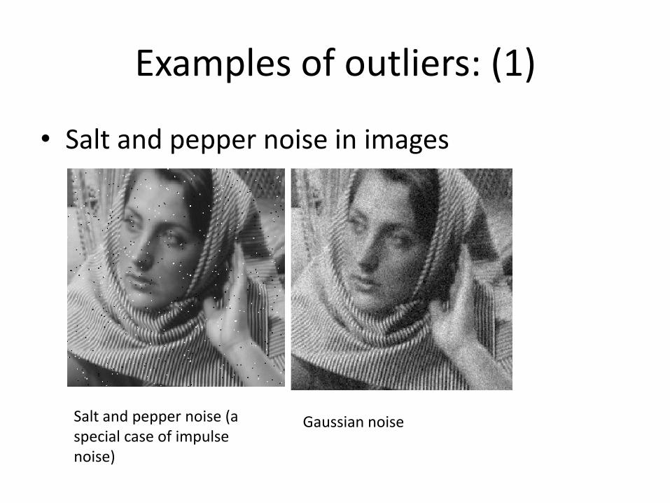
• Salt and pepper noise in images

Salt and pepper noise (a special case of impulse noise)

Gaussian noise

Examples of outliers: (2)

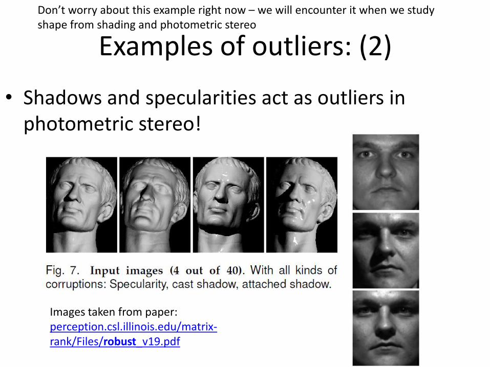
• Shadows and specularities act as outliers in photometric stereo!

Images taken from paper:perception.csl.illinois.edu/matrix-rank/Files/robust_v19.pdf‎

Don’t worry about this example right now – we will encounter it when we study shape from shading and photometric stereo

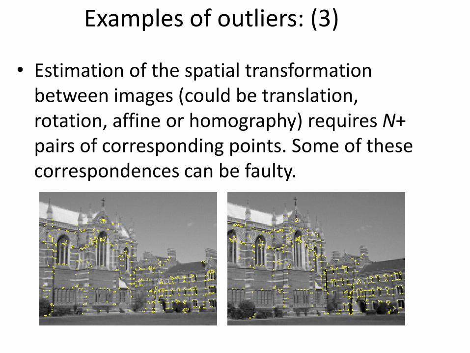
Examples of outliers: (3)

• Estimation of the spatial transformation between images (could be translation, rotation, affine or homography) requires N+ pairs of corresponding points. Some of these correspondences can be faulty.

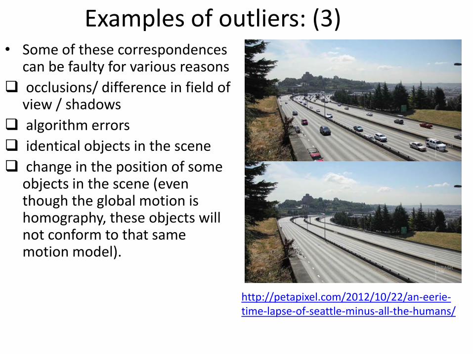
Examples of outliers: (3)• Some of these correspondences

can be faulty for various reasons

occlusions/ difference in field of view / shadows

algorithm errors

identical objects in the scene

change in the position of some objects in the scene (even though the global motion is homography, these objects will not conform to that same motion model).

http://petapixel.com/2012/10/22/an-eerie-time-lapse-of-seattle-minus-all-the-humans/

Examples of outliers: (4)

• The motion between consecutive frames of a video in the following link may be modeled as affine. But some corresponding pairs of points (example: on independently moving objects) don’t conform to that model – those are outliers.

https://www.youtube.com/watch?v=17VAuBL1Lxc

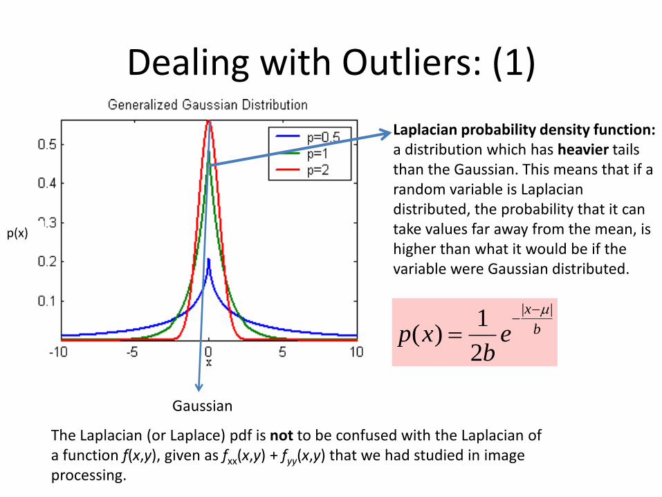
Dealing with Outliers: (1)

Laplacian probability density function: a distribution which has heavier tails than the Gaussian. This means that if a random variable is Laplacian distributed, the probability that it can take values far away from the mean, is higher than what it would be if the variable were Gaussian distributed.

b

x

eb

xp||

2

1)(

Gaussian

The Laplacian (or Laplace) pdf is not to be confused with the Laplacian of a function f(x,y), given as fxx(x,y) + fyy(x,y) that we had studied in image processing.

p(x)

Dealing with Outliers: (1)

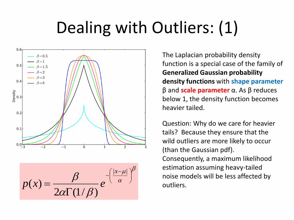
The Laplacian probability density function is a special case of the family of Generalized Gaussian probability density functions with shape parameter β and scale parameter α. As β reduces below 1, the density function becomes heavier tailed.

||

)/1(2)(

x

exp

Question: Why do we care for heavier tails? Because they ensure that the wild outliers are more likely to occur (than the Gaussian pdf). Consequently, a maximum likelihood estimation assuming heavy-tailed noise models will be less affected by outliers.

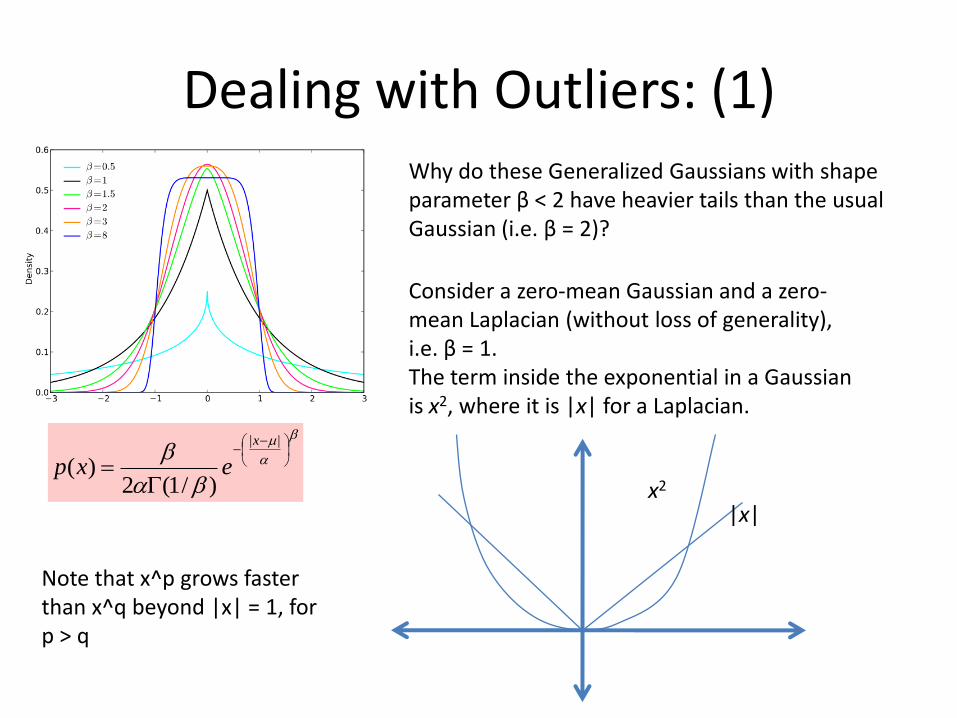
Dealing with Outliers: (1)Why do these Generalized Gaussians with shape parameter β < 2 have heavier tails than the usual Gaussian (i.e. β = 2)?

||

)/1(2)(

x

exp

Consider a zero-mean Gaussian and a zero-mean Laplacian (without loss of generality), i.e. β = 1.The term inside the exponential in a Gaussian is x2, where it is |x| for a Laplacian.

|x|x2

Note that x^p grows faster than x^q beyond |x| = 1, for p > q

Dealing with Outliers: (1)

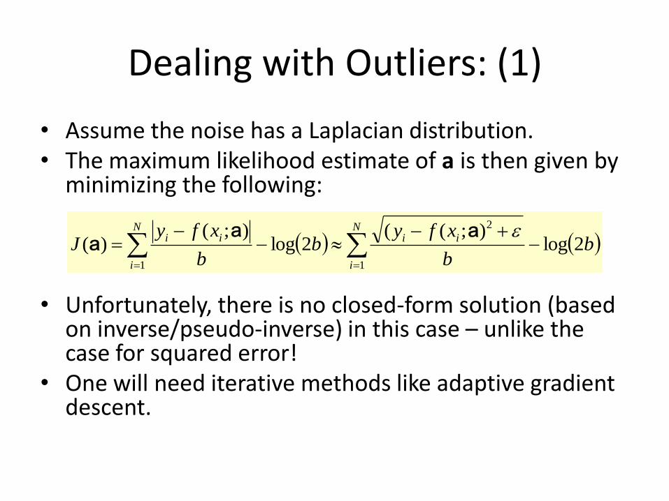
• Assume the noise has a Laplacian distribution.• The maximum likelihood estimate of a is then given by

minimizing the following:

• Unfortunately, there is no closed-form solution (based on inverse/pseudo-inverse) in this case – unlike the case for squared error!

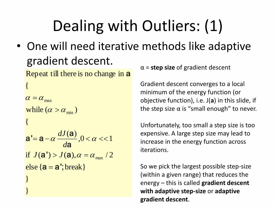
• One will need iterative methods like adaptive gradient descent.

bb

xfyb

b

xfyJ

N

i

iiN

i

ii 2log);((

2log);(

)(1

2

1

aaa

Dealing with Outliers: (1)• One will need iterative methods like adaptive

gradient descent.

}

}

break}{ else

2/),()( if

10,)(

{

)( while

{

in change no is therelRepeat til

max

min

max

;a 'a

aa '

a

aaa '

a

JJ

d

dJ

α = step size of gradient descent

Gradient descent converges to a local minimum of the energy function (or objective function), i.e. J(a) in this slide, if the step size α is “small enough” to never.

Unfortunately, too small a step size is too expensive. A large step size may lead to increase in the energy function across iterations.

So we pick the largest possible step-size (within a given range) that reduces the energy – this is called gradient descent with adaptive step-size or adaptive gradient descent.

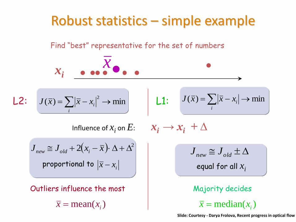
Robust statistics – simple example

Find “best” representative for the set of numbers

min)(2

i

ixxxJL2: min)( i

ixxxJL1:

xix

Influence of xi on E: xi → xi + ∆

)mean( ixx

Outliers influence the most

ixx proportional to

22 xxJJ ioldnew

)median( ixx

Majority decides

equal for all xi

oldnew JJ

Slide: Courtesy - Darya Frolova, Recent progress in optical flow

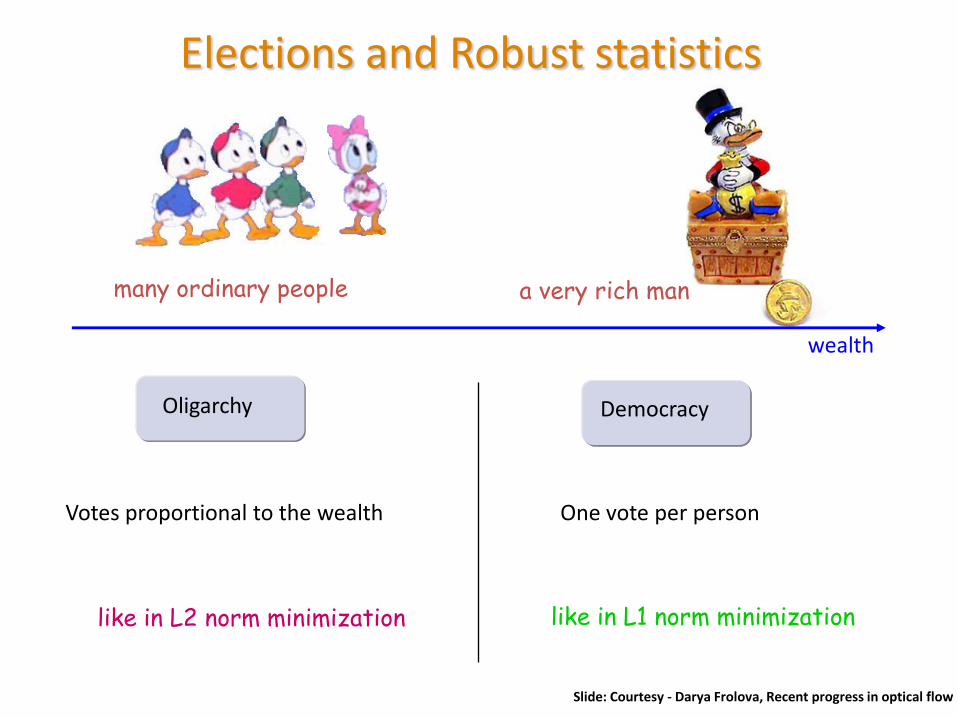
Elections and Robust statistics

many ordinary people a very rich man

Oligarchy

Votes proportional to the wealth

Democracy

One vote per person

wealth

like in L2 norm minimization like in L1 norm minimization

Slide: Courtesy - Darya Frolova, Recent progress in optical flow

New ways of defining the mean

• We know the mean as the one that minimizes the following quantity:

• Changing the error to sum of absolute values, we get:

n

x

n

x

E

n

i

i

n

i

i

11

2)(

)(

)}({

||

)( 11 n

ii

n

i

i

xmediann

x

E

We will prove this in class!

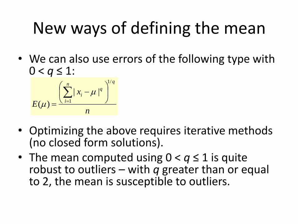
New ways of defining the mean

• We can also use errors of the following type with 0 < q ≤ 1:

• Optimizing the above requires iterative methods (no closed form solutions).

• The mean computed using 0 < q ≤ 1 is quite robust to outliers – with q greater than or equal to 2, the mean is susceptible to outliers.

n

x

E

qn

i

q

i

/1

1

||

)(

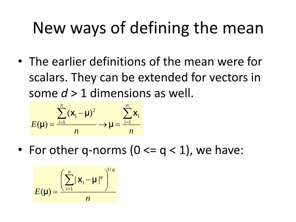
New ways of defining the mean

• The earlier definitions of the mean were for scalars. They can be extended for vectors in some d > 1 dimensions as well.

• For other q-norms (0 <= q < 1), we have:

nnE

n

i

n

i

11

2)(

)(ii x

μ

μx

μ

nE

qn

i

q

/1

1

||

)(

μx

μi

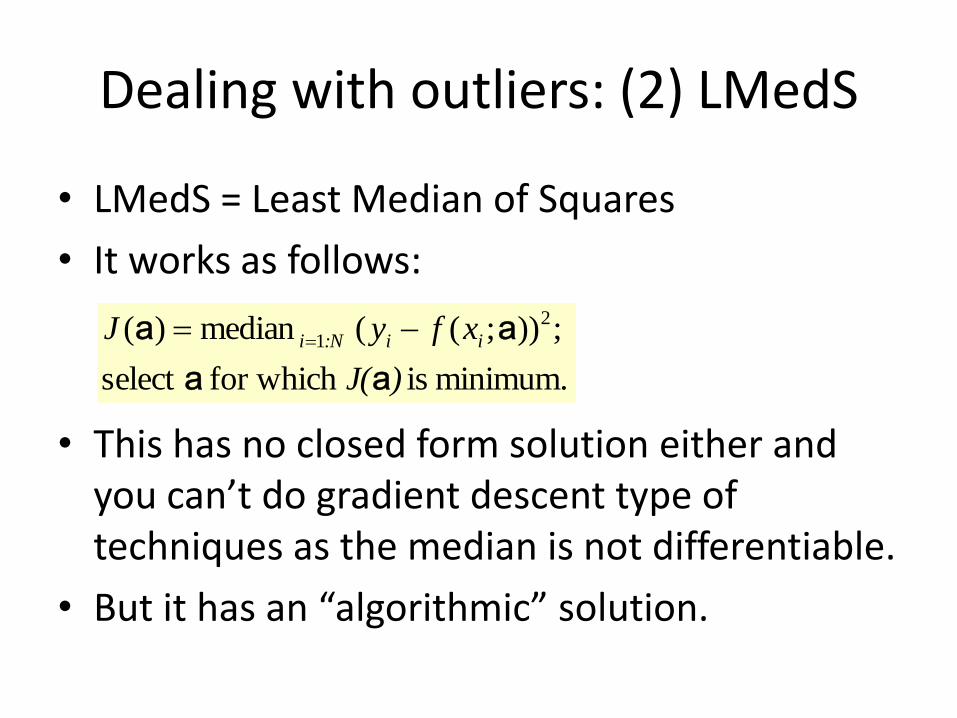
Dealing with outliers: (2) LMedS

• LMedS = Least Median of Squares

• It works as follows:

• This has no closed form solution either and you can’t do gradient descent type of techniques as the median is not differentiable.

• But it has an “algorithmic” solution.

minimum. is for which select

;));(( median)( 2

1

)J(

xfyJ ii:Ni

aa

aa

Dealing with outliers: (2) LMedS

• Step 1: Arbitrarily choose k out of N points where k is the smallest number of points required to determine a. Call this set of kpoints as C.

o Eg: If you had to do line fitting, k = ?

o Eg: If you were doing circle fitting, k = ?

o Eg: If you have to find the affine transformation between two point sets in 2D, you need k = ? correspondences.

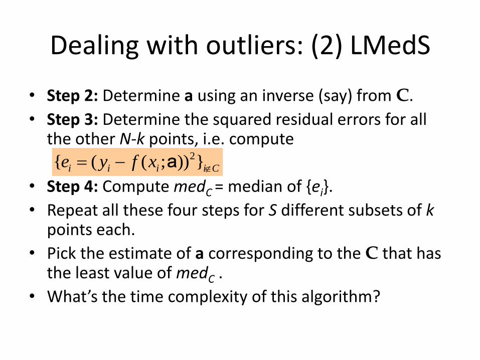
Dealing with outliers: (2) LMedS

• Step 2: Determine a using an inverse (say) from C.

• Step 3: Determine the squared residual errors for all the other N-k points, i.e. compute

• Step 4: Compute medC = median of {ei}.

• Repeat all these four steps for S different subsets of kpoints each.

• Pick the estimate of a corresponding to the C that has the least value of medC .

• What’s the time complexity of this algorithm?

Ciiii xfye }));(({ 2a

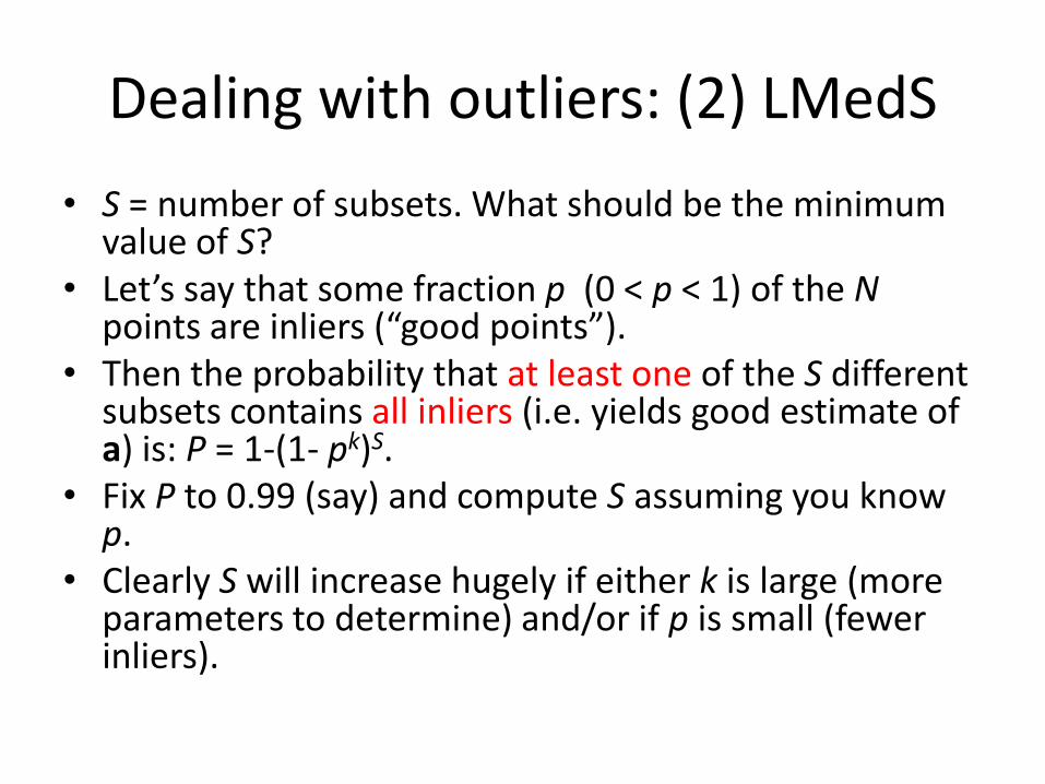
Dealing with outliers: (2) LMedS

• S = number of subsets. What should be the minimum value of S?

• Let’s say that some fraction p (0 < p < 1) of the Npoints are inliers (“good points”).

• Then the probability that at least one of the S different subsets contains all inliers (i.e. yields good estimate of a) is: P = 1-(1- pk)S.

• Fix P to 0.99 (say) and compute S assuming you know p.

• Clearly S will increase hugely if either k is large (more parameters to determine) and/or if p is small (fewer inliers).

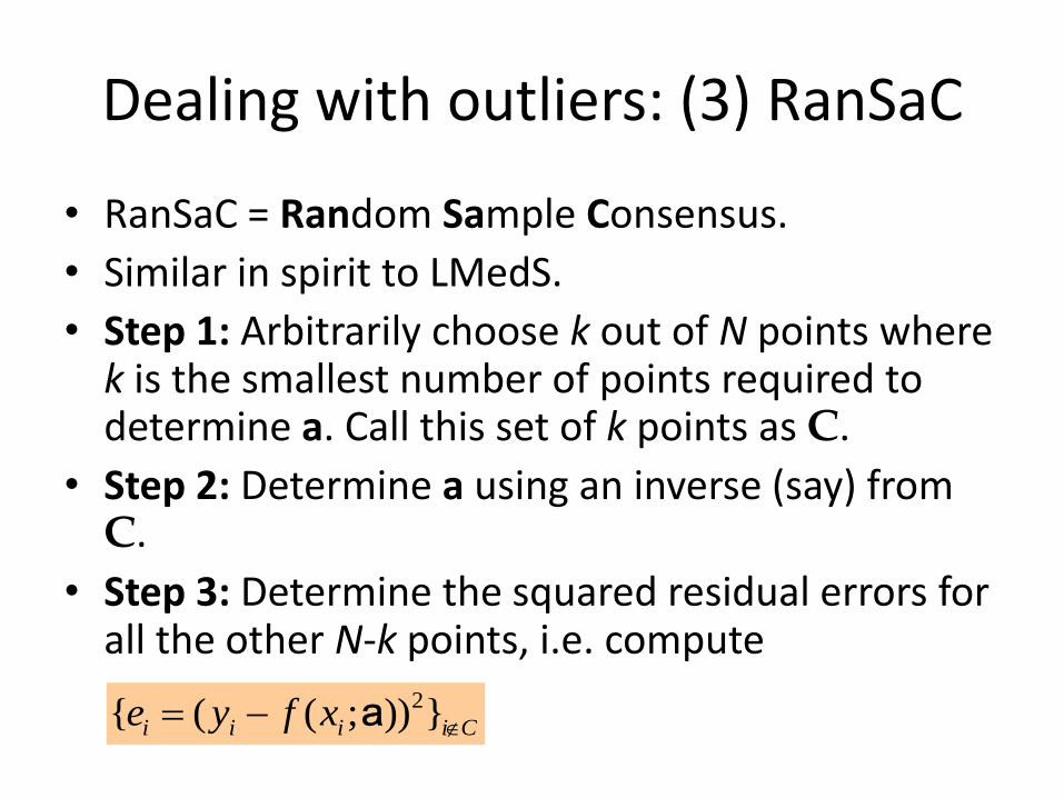
Dealing with outliers: (3) RanSaC

• RanSaC = Random Sample Consensus.

• Similar in spirit to LMedS.

• Step 1: Arbitrarily choose k out of N points where k is the smallest number of points required to determine a. Call this set of k points as C.

• Step 2: Determine a using an inverse (say) from C.

• Step 3: Determine the squared residual errors for all the other N-k points, i.e. compute

Ciiii xfye }));(({ 2a

Dealing with outliers: (3) RanSaC

• Step 4: Count the number of points for which ei < threshold λ. These points form the “consensus set” for the chosen model.

• Repeat all 4 steps for multiple subsets and pick the subset which has maximum number of inliers and its corresponding estimate of a.

• Choice of S – same as LMedS.

Sample result with RanSaC for line fitting.

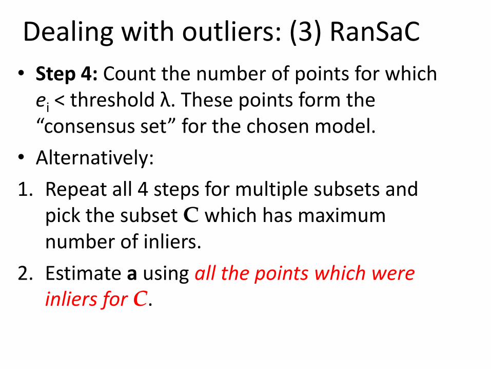
Dealing with outliers: (3) RanSaC

• Step 4: Count the number of points for which ei < threshold λ. These points form the “consensus set” for the chosen model.

• Alternatively:

1. Repeat all 4 steps for multiple subsets and pick the subset C which has maximum number of inliers.

2. Estimate a using all the points which were inliers for C.

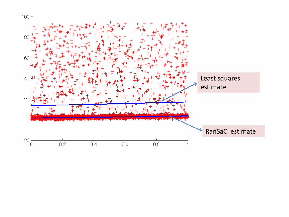
Least squares estimate

RanSaC estimate

RANSAC versus LMedS

• LMedS needs no threshold to determine what is an inlier unlike RanSaC.

• But RanSaC has one advantage. What?

o LMedS will need at least 50% inliers (by definition of median).

o RanSaC can tolerate a smaller percentage of inliers (i.e. larger percentage of outliers).

Expected number of RanSaC iterations

• The probability that at least one point in a chosen set of k points is an outlier = 1-pk.

• The probability that the i-th set is the first set that contains no outliers = (1-pk)i-1pk to be denoted as Q(i).

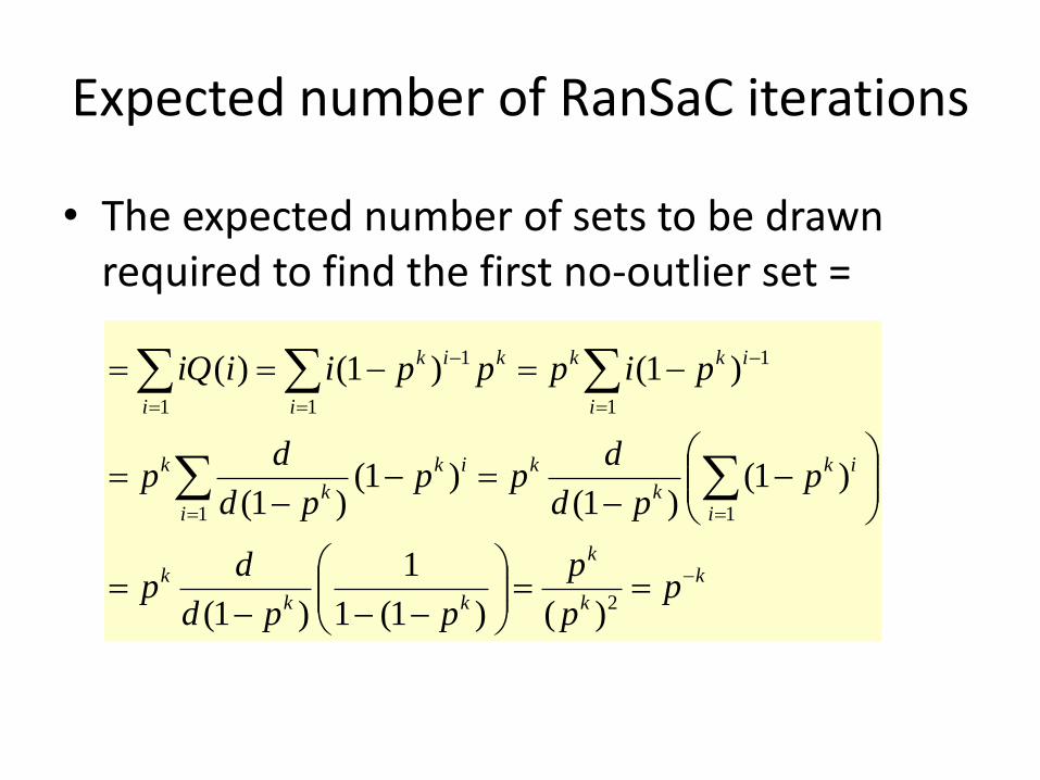
Expected number of RanSaC iterations

• The expected number of sets to be drawn required to find the first no-outlier set =

k

k

k

kk

k

i

ik

k

k

i

ik

k

k

i

ikk

i

kik

i

pp

p

ppd

dp

ppd

dpp

pd

dp

pipppiiiQ

2

11

1

1

1

1

1

)()1(1

1

)1(

)1()1(

)1()1(

)1()1()(

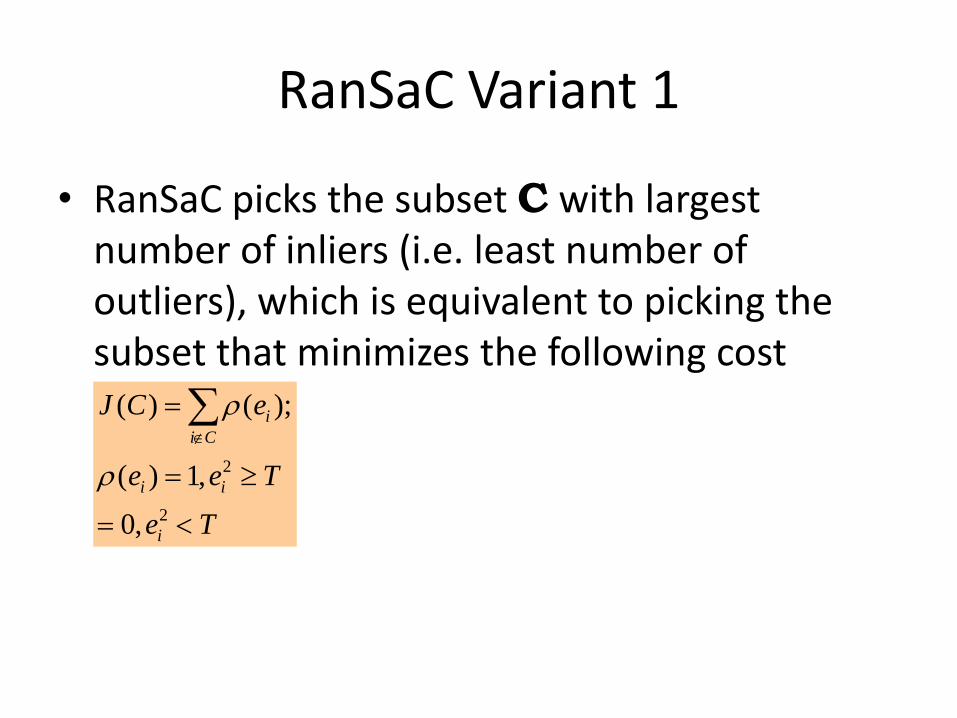
RanSaC Variant 1

• RanSaC picks the subset C with largest number of inliers (i.e. least number of outliers), which is equivalent to picking the subset that minimizes the following cost function:

Te

Tee

eCJ

i

ii

Ci

i

2

2

,0

,1)(

);()(

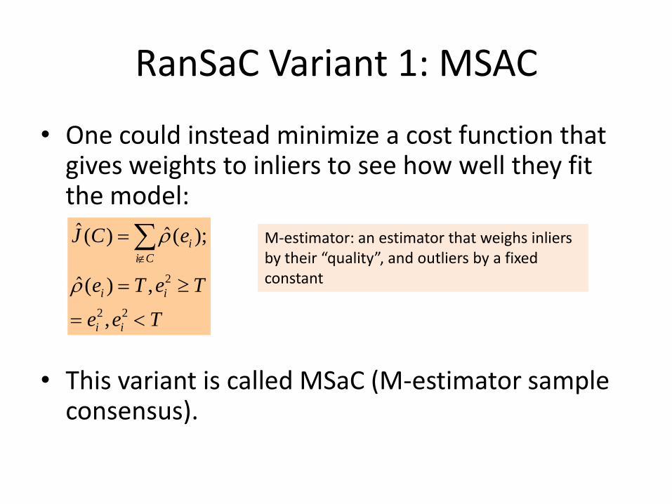
RanSaC Variant 1: MSAC

• One could instead minimize a cost function that gives weights to inliers to see how well they fit the model:

• This variant is called MSaC (M-estimator sample consensus).

Tee

TeTe

eCJ

ii

ii

Ci

i

22

2

,

,)(ˆ

);(ˆ)(ˆ

M-estimator: an estimator that weighs inliers by their “quality”, and outliers by a fixed constant

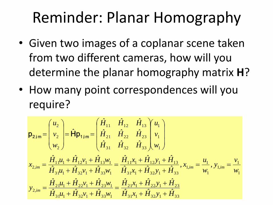
Reminder: Planar Homography

• Given two images of a coplanar scene taken from two different cameras, how will you determine the planar homography matrix H?

• How many point correspondences will you require?

33132131

23122121

133132131

123122121,2

1

1,1

1

1,1

33132131

13112111

133132131

113112111,2

1

1

1

333231

232221

131211

2

2

2

ˆˆˆ

ˆˆˆ

ˆˆˆ

ˆˆˆ

,,ˆˆˆ

ˆˆˆ

ˆˆˆ

ˆˆˆ

ˆˆˆ

ˆˆˆ

ˆˆˆ

ˆ

HyHxH

HyHxH

wHvHuH

wHvHuHy

w

vy

w

ux

HyHxH

HyHxH

wHvHuH

wHvHuHx

w

v

u

HHH

HHH

HHH

w

v

u

im

imimim

i m1 ,i m2 , pHp

Planar Homography

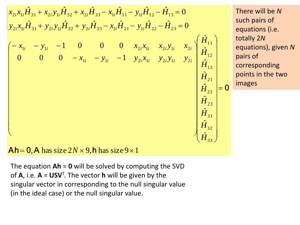
• Rearranging these equations, we get:

There will be Nsuch pairs of equations (i.e. totally 2Nequations), given Npairs of corresponding points in the two images

The equation Ah = 0 will be solved by computing the SVD of A, i.e. A = USVT. The vector h will be given by the singular vector in corresponding to the null singular value (in the ideal case) or the null singular value.

19 size has ,92 size has ,

ˆ

ˆ

ˆ

ˆ

ˆ

ˆ

ˆ

ˆ

ˆ

1000

0001

0ˆˆˆˆˆˆ

0ˆˆˆˆˆˆ

33

32

31

23

22

21

13

12

11

2121211

2121211

2322121133232123112

1312111133232123112

hA0Ah

0

N

H

H

H

H

H

H

H

H

H

yyyxyyx

xyxxxyx

HHyHxHyHyyHxy

HHyHxHxHyxHxx

iiiiiii

iiiiiii

iiiiiii

iiiiiii

Application: RANSAC to determine Homography between two Images

• Determine sets Q1 and Q2 of salient feature points in both images, using the SIFT algorithm.

• Q1 and Q2 may have different sizes! Determine the matching points between Q1and Q2 using methods such as matching of SIFT descriptors.

• Many of these matches will be near-accurate, but there will be outliers too!

Application: RANSAC to determine Homography between two Images

• Pick a set of any k = 4 pairs of points and determine homography matrix H using SVD based method.

• Determine the number of inliers – i.e. those point pairs for which:

• Select the estimate of H corresponding to the set that yielded maximum number of inliers!

2

221 ii Hqq

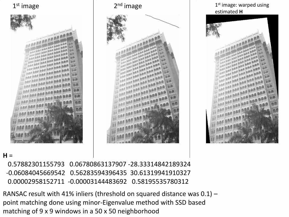
H =0.57882301155793 0.06780863137907 -28.33314842189324

-0.06084045669542 0.56283594396435 30.613199419103270.00002958152711 -0.00003144483692 0.58195535780312

RANSAC result with 41% inliers (threshold on squared distance was 0.1) –point matching done using minor-Eigenvalue method with SSD based matching of 9 x 9 windows in a 50 x 50 neighborhood

1st image 2nd image 1st image: warped using estimated H

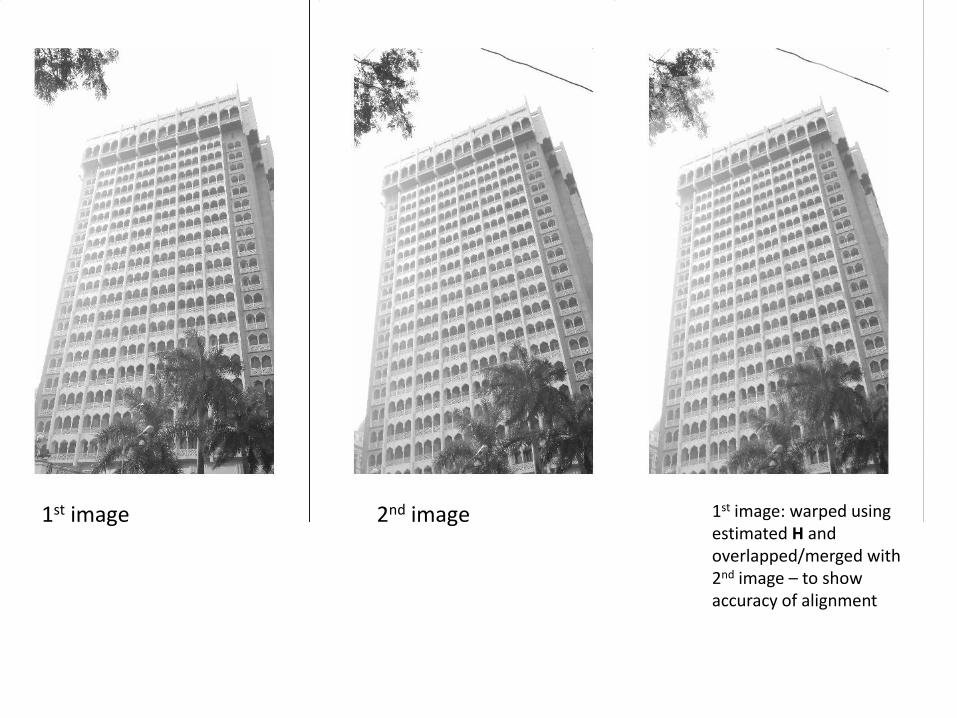
1st image 2nd image 1st image: warped using estimated H and overlapped/merged with 2nd image – to show accuracy of alignment

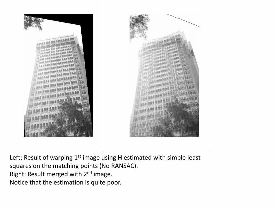
Left: Result of warping 1st image using H estimated with simple least-squares on the matching points (No RANSAC). Right: Result merged with 2nd image.Notice that the estimation is quite poor.

Some cautions with RANSAC• Consider a dataset with a cloud of points all

close to each other (degenerate set). A model created from an outlier point and any point from a degenerate set will have a large consensus set!

Image taken from Ph.D. thesis of OndrejChum, Czech Technical University, Prague

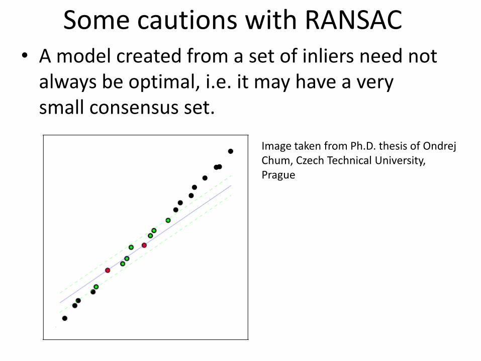
Some cautions with RANSAC• A model created from a set of inliers need not

always be optimal, i.e. it may have a very small consensus set.

Image taken from Ph.D. thesis of OndrejChum, Czech Technical University, Prague

References

• Appendix A.7 of Trucco and Verri

• Article on Robust statistics by Chuck Stewart

• Original article on RanSaC by Fischler and Bolles

• Article on RanSaC variants by Torr and Zisserman