Robust Estimation of 3D Human Poses from a Single Image

Chunyu Wang1,2, Yizhou Wang1,2, Zhouchen Lin2, Alan L. Yuille3, and Wen Gao1

1Nat’l Engineering Lab for Video Technology, Sch’l of EECS, Peking University, Beijing, China2Key Lab. of Machine Perception (MOE), Sch’l of EECS, Peking University, Beijing, China

3Department of Statistics, University of California, Los Angeles (UCLA), USA

Abstract

Human pose estimation is a key step to action recogni-tion. We propose a method of estimating 3D human posesfrom a single image, which works in conjunction with anexisting 2D pose/joint detector. 3D pose estimation is chal-lenging because multiple 3D poses may correspond to thesame 2D pose after projection due to the lack of depth in-formation. Moreover, current 2D pose estimators are usu-ally inaccurate which may cause errors in the 3D estima-tion. We address the challenges in three ways: (i) We rep-resent a 3D pose as a linear combination of a sparse set ofbases learned from 3D human skeletons. (ii) We enforcelimb length constraints to eliminate anthropomorphicallyimplausible skeletons. (iii) We estimate a 3D pose by mini-mizing the L1-norm error between the projection of the 3Dpose and the corresponding 2D detection. The L1-normloss term is robust to inaccurate 2D joint estimations. Weuse the alternating direction method (ADM) to solve the op-timization problem efficiently. Our approach outperformsthe state-of-the-arts on three benchmark datasets.

1. Introduction

Action recognition is a key problem in computer vision[19] and has many applications such as human-computerinteraction and video surveillance. Since an action is nat-urally represented by human poses [18], 2D and 3D poseestimation has attracted a lot of attention. A 2D pose isusually represented by a set of joint locations [21] whoseestimation remains challenging because of the huge humanappearance variation, viewpoint change, etc.

A 3D pose is typically represented by a skeleton modelparameterized by joint locations [16] or by rotation angles[8]. The representation is intrinsic as it is invariant to view-point changes. However, estimating 3D poses from a singleimage remains a difficult problem. First, a 3D pose is usu-

Input Image 2D Pose

M1

M2

3D Pose Camera

(1)

(2)

(3)

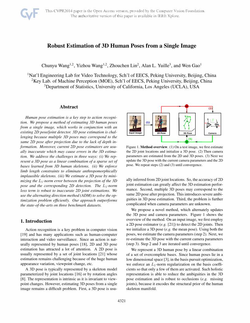
Figure 1. Method overview. (1) On a test image, we first estimatethe 2D joint locations and initialize a 3D pose. (2) Then cameraparameters are estimated from the 2D and 3D poses. (3) Next weupdate the 3D pose with the current camera parameters and the 2Dpose. We repeat steps (2) and (3) until convergence.

ally inferred from 2D joint locations. So, the accuracy of 2Djoint estimation can greatly affect the 3D estimation perfor-mance. Second, multiple 3D poses may correspond to thesame 2D pose after projection. This introduces severe ambi-guities in 3D pose estimation. Third, the problem is furthercomplicated when camera parameters are unknown.

We propose a novel method, which alternately updatesthe 3D pose and camera parameters. Figure 1 shows theoverview of the method. On an input image, we first employa 2D pose estimator (e.g. [21]) to detect the 2D joints. Thenwe initialize a 3D pose (e.g. the mean pose). Using both theposes, we estimate the camera parameters (step 2). Next, were-estimate the 3D pose with the current camera parameters(step 3). Step 2 and 3 are iterated until convergence.

We represent a 3D human pose by a linear combinationof a set of overcomplete bases. Since human poses lie in alow dimensional space [3], in the basis pursuit optimization,we enforce an L1-norm regularization on the basis coeffi-cients so that only a few of them are activated. Such holisticrepresentation is able to reduce the ambiguities in the 3Dpose estimation and is robust to occlusions (e.g. missingjoints), because it encodes the structural prior of the humanskeleton manifold.

4321

We estimate a 3D pose (i.e. basis coefficients) by min-imizing an L1-norm penalty between the projection of the3D joints and the 2D detections. The commonly used L2-norm tends to distribute errors evenly over all variables.When some joints of the estimated 2D pose are inaccurate,the inferred 3D pose may be biased to a completely wrongconfiguration. In contrast, L1-norm is more tolerant to theinaccurate 2D joints. However, even if the L1-norm error isadopted, the inferred 3D skeleton may still violate the an-thropometric quantities such as limb proportions. Hence,we enforce eight limb length constraints on the estimated3D pose to eliminate the incorrect ones.

We use an efficient alternating direction method (ADM)to solve our optimization problem. Although global opti-mality is not guaranteed, we obtain reasonably good solu-tions. Our method outperforms the state-of-the-arts on threebenchmark datasets.

The paper is organized as follows. Section 2 reviews therelated work. Section 3 introduces the proposed approach.Section 4 shows implementation details and experiment re-sults. Conclusion is in section 5. Section 6 (Appendix)presents the optimization method in detail.

2. Related WorkExisting work on 3D pose estimation can be classified

into four categories according to their inputs to the system,e.g. the image, image features, camera parameters, etc. Thefirst class [7] [15] takes camera parameters as inputs. Forexample, Lee et al. [7] represent a 3D pose by a skeletonmodel and parameterize the body parts by truncated cones.They estimate the rotation angles of body parts by minimiz-ing the silhouette discrepancy between the model projec-tions and the input image by applying Markov Chain MonteCarlo (MCMC). Simo-Serra et al. [15] represent a 3D poseby a set of joint locations. They automatically estimate the2D pose, model each joint by a Gaussian distribution, andpropagate the uncertainty to 3D pose space. They samplea set of 3D skeletons from the space and learn a SVM todetermine the most feasible one.

The second class [17] [20] requires manually labeled 2Djoint locations in a video as input. Valmadre et al. [17] firstapply structure from motion to estimate the camera param-eters and the 3D pose of the rigid torso, and then requirehuman input to resolve the depth ambiguities for non-torsojoints. Wei et al. [20] propose the “rigid body constraints”,e.g. the pelvis, left and right hip joints form a rigid struc-ture, and require that the distance between any two joints onthe rigid structure remains unchanged across time. They es-timate the 3D poses by minimizing the discrepancy betweenthe projection of the 3D poses and the 2D joint detectionswithout violating the “rigid body constraints”.

The third class [16] [12] requires manually labeled 2Djoints in one image. Taylor [16] assumes that the limb

lengths are known and calculates the relative depths of thelimbs by considering foreshortening. It requires human in-put to resolve the depth ambiguities at each joint. Ramakr-ishna et al. [12] represent a 3D pose by a linear combinationof a set of bases. They split the training data into classes,apply PCA to each class, and combine the principal compo-nents as bases. They greedily add the most correlated basisinto the model and estimate the coefficients by minimizingan L2-norm error between the projection of 3D pose andthe 2D pose. They enforce a constraint on the sum of thelimb lengths, which is just a weak constraint. This work[12] achieves the state-of-the-art performance but relies onmanually labeled 2D joint locations.

The fourth class [11] [3] requires only a single image orimage features (e.g. silhouettes). For example, Mori et al.[11] match a test image to the stored exemplars using shapecontext descriptors, and transfer the matched 2D pose to thetest image. They lift the 2D pose to 3D using the methodproposed in [16]. Elgammal et al.[3] propose to learn view-based silhouettes manifolds and the mapping function fromthe manifold to 3D poses. These approaches do not explic-itly estimate camera parameters, but require a lot of trainingdata from various viewpoints.

Our method requires only a single image to infer 3D hu-man poses. It is similar to [12] but there are five distinctivedifferences. (i) We obtain 2D joint locations by running adetector [21] rather than by manual labeling. (ii) We useL1-norm penalty instead of the L2-norm one as it is morerobust to inaccurate 2D joint locations. (iii) They [12] en-force a weak anthropomorphic constraint (i.e. sum of limblength) for the sake of computational simplicity, which isinsufficient to eliminate incorrect poses; while we enforceeight limb length constraints, which is much more effec-tive. (iv) We enforce an L1-norm constraint on the basis co-efficients rather than greedily adding bases into the modelto encourage sparsity. They need to re-estimate the coeffi-cients every time a new basis is introduced, which is ineffi-cient. (v) We use an efficient alternating direction methodto solve our optimization problem.

3. Our Approach

We represent 2D and 3D poses by n joint locationsx ∈ R2n and y ∈ R3n, respectively. By assuming a weakperspective camera model, the 2D projection x of a 3D posey in an image are related as: x = My, whereM = In⊗M0,in which I is the identity matrix, ⊗ is the Kronecker prod-

uct, and M0 =

(mT

1

mT2

)∈ R2×3 is the camera projection

matrix. Given the estimated x, we alternately estimate thecamera parameter M0 and the 3D pose y. We describe thedetails for 3D pose estimation in section 3.1 and for cameraparameter estimation in section 3.2.

3.1. Robust 3D Pose Estimation

We represent a 3D pose y as a linear combination of aset of bases B = b1, · · · , bk, i.e. y =

∑ki=1 αi · bi + µ,

where α are the basis coefficients and µ is the mean pose.Given a 2D pose x and camera parameter M0, we estimatethe coefficients α by minimizing an L1-norm error betweenthe projection of the estimated 3D pose and the 2D pose:‖M (Bα+ µ)− x‖1. We also enforce L1-norm regulariza-tion on the basis coefficients α and eight limb length con-straints on the inferred 3D pose.

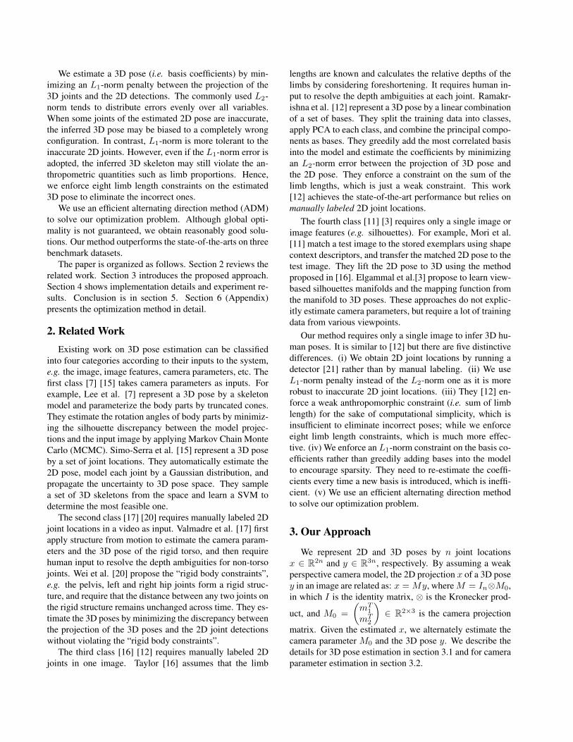
(a) (b) (c)Figure 2. Comparison of 3D pose estimation by minimizing L1-norm vs L2-norm penalty. (a) estimated 2D joint locations wherethe right foot location is inaccurate. (b-c) are the estimated 3Dposes using the L1-norm and L2-norm, respectively. The L2-normpenalty biases the estimation to a wrong pose.

3.1.1 L1-norm Objective Function

L2-norm is the most widely used error metric in the liter-ature. However, it is sensitive to inaccuracies in 2D poseestimation, which are usually caused by failures in featuredetections and other factors, because it tends to distributeerrors uniformly. In this work, we propose to minimize anL1-norm error, i.e. ‖x−M(Bα+ µ)‖1. As a widely usedrobust regularizer in statistics, the L1 penalty is robust to in-accurate 2D joint outliers. For example, in Figure 2 the 2Dlocation of the right foot is inaccurate. The estimated 3Dpose using L2-norm error is drastically biased to a wrongconfiguration. The camera parameter estimation is also in-correct. However, using L1-norm returns a reasonable 3Dpose. Extensive experiments on benchmark datasets justifythat using the L1-norm can improve the performance, espe-cially when 2D pose estimation is inaccurate.

3.1.2 Sparsity Constraint on the Basis Coefficients

Although human poses are highly variant, they lie in a lowdimensional space [13]. Hence, we enforce sparsity on thebasis coefficients α so that each 3D pose is represented byonly a few bases. The sparsity can be induced by minimiz-ing the L1-norm of α. This is an important structural priorto remove incorrect or anthropomorphically implausible 3Dposes. In addition, the sparsity constraint can also preventoverfitting to (inaccurate) 2D pose estimations. If there isno sparsity constraint, given a large number of bases we can

always decrease the projection error to zero for an arbitrary2D pose; however, there is no guarantee that the resulted 3Dpose is correct. In experiments, we observe that the sparsityconstraint is quite important. In summary, the resulted ob-jective function is:

minα

‖x−M (Bα+ µ)‖1 + θ ‖α‖1 (1)

where θ > 0 is a parameter that balances the loss term andthe regularization term.

3.1.3 Anthropomorphic Constraints

We require that the eight limb lengths of a 3D pose complywith certain proportions [6]. The eight limbs are left/right-upper/lower-arm/leg. We define a joint selection matrixEj = [0, · · · , I, · · · , 0] ∈ R3×3n, where the jth block isthe identity matrix. The product of Ej and y is the 3D loca-tion of the jth joint in pose y. Let Ci = Ei1 − Ei2 . Then‖Ciy‖22 is the squared length of the ith limb whose ends arethe i1-th and i2-th joints.

We normalize the length of the right lower leg to oneand compute the squared lengths of other limbs (say Li) ac-cording to the limb proportions used in [6]. The proportionsare kept the same for all people. Now we have constraints‖Ci (Bα+ µ)‖22 = Li. Given the camera parameters wecan formulate the 3D pose estimation problem as follows:

minα

‖x−M (Bα+ µ)‖1 + θ ‖α‖1

s.t. ‖Ci (Bα+ µ)‖22 = Li, i = 1, · · · , t(2)

3.2. Robust Camera Parameter Estimation

Given a 3D pose, we estimate the camera parameters byminimizing the L1-norm projection error. We reshape the2D and 3D poses, x and y, as X ∈ R2×n and Y ∈ R3×n,respectively. Then ideally X = M0Y should hold, where

M0 =

(mT

1

mT2

)is the projection matrix of a weak projec-

tive camera, i.e. mT1m2 = 0. Due to errors, we estimate

the camera parameters m1 and m2 by solving the followingproblem:

minm1,m2

∥∥∥∥X − ( mT1

mT2

)Y

∥∥∥∥1

, s.t. mT1m2 = 0. (3)

3.3. Optimization

We alternately update the 3D pose and the camera pa-rameters. We first initialize the 3D pose X by the meanpose of the training data, and estimate camera parametersm1 and m2 by solving problem (3). With the updated cam-era parameters, we then re-estimate the 3D pose by solvingproblem (2). We repeat the above process until convergenceor the maximum number of iterations is reached. We use thealternating direction method to solve the two optimizationproblems efficiently. Please see Appendix for details.

0 50 100 1500

0.5

1

1.5

2

2.5

Number of bases

Rec

on

stru

ctio

n e

rro

r

PCAClasswise PCASparse bases

(a)

0 20 40 600

0.2

0.4

0.6

0.8

1

Activated basis number

Pro

bab

ility

PCAClasswise PCASparse bases

(b)

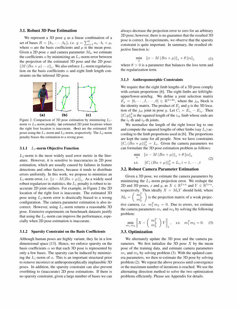
Figure 3. Comparison of the three basis learning methods on theCMU dataset. (a) 3D pose reconstruction errors using differentnumber of bases. (b) Cumulative distribution of the number ofactivated bases in represent the 3D poses. The y-axis is the per-centage of the cases whose activated basis number is less than orequal to the corresponding x-axis value on the curves.

4. The Experimental Results

We conduct two types of experiments to evaluate our ap-proach. The first type is controlled. We assume that the 2Djoint locations are known and evaluate the influence: (i) ofthe three factors (i.e. the sparsity term, the anthropomor-phic constraints and the L1-norm penalty), (ii) of the inac-curate 2D pose estimations and (iii) of the human-cameraangles, on the 3D pose estimation performance. The sec-ond type is real. We estimate the 2D pose in an image by adetector [21] and then estimate the 3D skeletons. We com-pare our method with the state-of-the-art ones [12] [15] [2].Our approach can also refine the 2D pose estimation by pro-jecting the estimated 3D pose to 2D image.

We use 12 body joints, i.e. the left and right shoulders,elbows, hands, hips, knees and feet, being consistent withthe 2D pose detector [21]. 200 bases are used for all exper-iments and about 6 of them are activated for representing a3D pose. In optimization, we terminate the algorithm if thenumber of iterations exceeds 20.

4.1. The Datasets

We evaluate our approach on three datasets: the CMUmotion dataset [1], the HumanEva dataset [14] and the UvA3D pose dataset [5]. For the CMU dataset, we learn thebases on actions of “climb”, “swing”, “sit” and “jump”,and test on different actions of “walk”, “run”, “golf” and“punch” to justify the generalization ability of our method.For the HumanEva dataset, we use the walking and joggingactions of three subjects for evaluation as in [15]. For theUvA dataset, we use the first four sequences for training andthe remaining eight for testing.

4.2. Basis Learning

Our approach pursues a set of sparse bases by enforc-ing an L1-norm regularization on the basis coefficients (asin [10]). But we also compare with other two basis learn-

0.0 2.0 4.0 6.0 8.0 10.0reconstruction error

0.0

0.2

0.4

0.6

0.8

1.0

accu

mul

ated

pro

babi

lity

L1WAWSL1WANSL1NAWSL1NANSL2WANSL2NANSL2WAWSL2NAWS

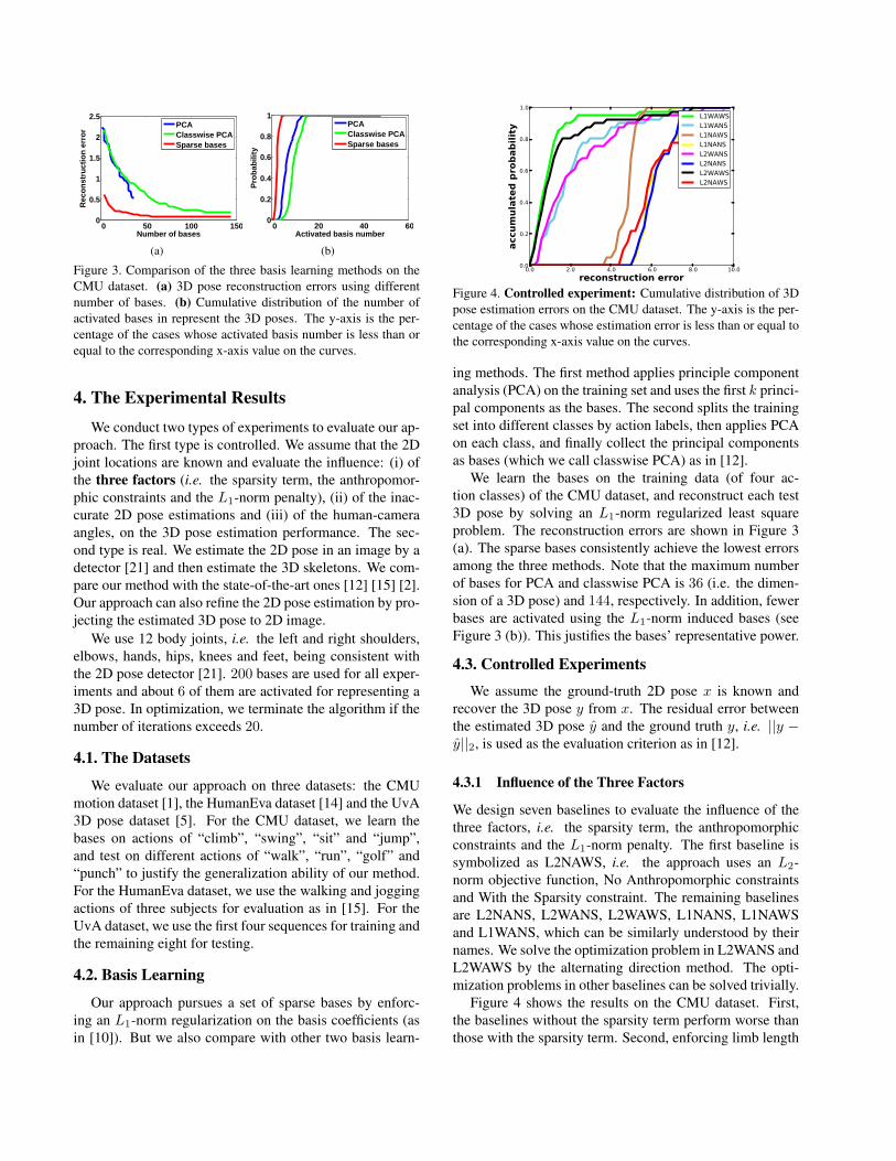
Figure 4. Controlled experiment: Cumulative distribution of 3Dpose estimation errors on the CMU dataset. The y-axis is the per-centage of the cases whose estimation error is less than or equal tothe corresponding x-axis value on the curves.

ing methods. The first method applies principle componentanalysis (PCA) on the training set and uses the first k princi-pal components as the bases. The second splits the trainingset into different classes by action labels, then applies PCAon each class, and finally collect the principal componentsas bases (which we call classwise PCA) as in [12].

We learn the bases on the training data (of four ac-tion classes) of the CMU dataset, and reconstruct each test3D pose by solving an L1-norm regularized least squareproblem. The reconstruction errors are shown in Figure 3(a). The sparse bases consistently achieve the lowest errorsamong the three methods. Note that the maximum numberof bases for PCA and classwise PCA is 36 (i.e. the dimen-sion of a 3D pose) and 144, respectively. In addition, fewerbases are activated using the L1-norm induced bases (seeFigure 3 (b)). This justifies the bases’ representative power.

4.3. Controlled Experiments

We assume the ground-truth 2D pose x is known andrecover the 3D pose y from x. The residual error betweenthe estimated 3D pose y and the ground truth y, i.e. ||y −y||2, is used as the evaluation criterion as in [12].

4.3.1 Influence of the Three Factors

We design seven baselines to evaluate the influence of thethree factors, i.e. the sparsity term, the anthropomorphicconstraints and the L1-norm penalty. The first baseline issymbolized as L2NAWS, i.e. the approach uses an L2-norm objective function, No Anthropomorphic constraintsand With the Sparsity constraint. The remaining baselinesare L2NANS, L2WANS, L2WAWS, L1NANS, L1NAWSand L1WANS, which can be similarly understood by theirnames. We solve the optimization problem in L2WANS andL2WAWS by the alternating direction method. The opti-mization problems in other baselines can be solved trivially.

Figure 4 shows the results on the CMU dataset. First,the baselines without the sparsity term perform worse thanthose with the sparsity term. Second, enforcing limb length

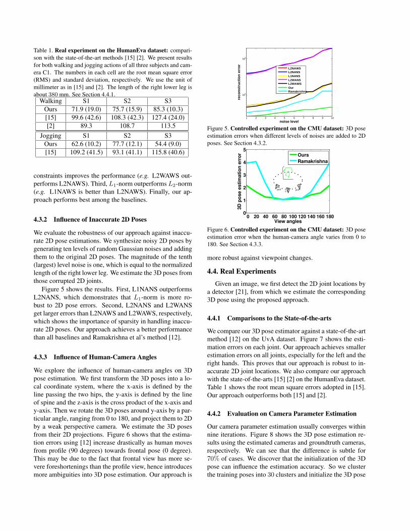
Table 1. Real experiment on the HumanEva dataset: compari-son with the state-of-the-art methods [15] [2]. We present resultsfor both walking and jogging actions of all three subjects and cam-era C1. The numbers in each cell are the root mean square error(RMS) and standard deviation, respectively. We use the unit ofmillimeter as in [15] and [2]. The length of the right lower leg isabout 380 mm. See Section 4.4.1.

Walking S1 S2 S3Ours 71.9 (19.0) 75.7 (15.9) 85.3 (10.3)[15] 99.6 (42.6) 108.3 (42.3) 127.4 (24.0)[2] 89.3 108.7 113.5

Jogging S1 S2 S3Ours 62.6 (10.2) 77.7 (12.1) 54.4 (9.0)[15] 109.2 (41.5) 93.1 (41.1) 115.8 (40.6)

constraints improves the performance (e.g. L2WAWS out-performs L2NAWS). Third, L1-norm outperforms L2-norm(e.g. L1NAWS is better than L2NAWS). Finally, our ap-proach performs best among the baselines.

4.3.2 Influence of Inaccurate 2D Poses

We evaluate the robustness of our approach against inaccu-rate 2D pose estimations. We synthesize noisy 2D poses bygenerating ten levels of random Gaussian noises and addingthem to the original 2D poses. The magnitude of the tenth(largest) level noise is one, which is equal to the normalizedlength of the right lower leg. We estimate the 3D poses fromthose corrupted 2D joints.

Figure 5 shows the results. First, L1NANS outperformsL2NANS, which demonstrates that L1-norm is more ro-bust to 2D pose errors. Second, L2NANS and L2WANSget larger errors than L2NAWS and L2WAWS, respectively,which shows the importance of sparsity in handling inaccu-rate 2D poses. Our approach achieves a better performancethan all baselines and Ramakrishna et al’s method [12].

4.3.3 Influence of Human-Camera Angles

We explore the influence of human-camera angles on 3Dpose estimation. We first transform the 3D poses into a lo-cal coordinate system, where the x-axis is defined by theline passing the two hips, the y-axis is defined by the lineof spine and the z-axis is the cross product of the x-axis andy-axis. Then we rotate the 3D poses around y-axis by a par-ticular angle, ranging from 0 to 180, and project them to 2Dby a weak perspective camera. We estimate the 3D posesfrom their 2D projections. Figure 6 shows that the estima-tion errors using [12] increase drastically as human movesfrom profile (90 degrees) towards frontal pose (0 degree).This may be due to the fact that frontal view has more se-vere foreshortenings than the profile view, hence introducesmore ambiguities into 3D pose estimation. Our approach is

1 2 3 4 5 6 7 8 9 10

101

102

noise level

reco

nst

ruct

ion

err

or

L2NAWSL2NANSL1NANSL2WANSL2WAWSOurRamakrishna

Figure 5. Controlled experiment on the CMU dataset: 3D poseestimation errors when different levels of noises are added to 2Dposes. See Section 4.3.2.

0pi/4-pi/4

0 20 40 60 80 100 120 140 160 1800

1

2

3

4

5

View angles

3D p

ose

estim

atio

n er

ror Ours

Ramakrishna

Figure 6. Controlled experiment on the CMU dataset: 3D poseestimation error when the human-camera angle varies from 0 to180. See Section 4.3.3.

more robust against viewpoint changes.

4.4. Real Experiments

Given an image, we first detect the 2D joint locations bya detector [21], from which we estimate the corresponding3D pose using the proposed approach.

4.4.1 Comparisons to the State-of-the-arts

We compare our 3D pose estimator against a state-of-the-artmethod [12] on the UvA dataset. Figure 7 shows the esti-mation errors on each joint. Our approach achieves smallerestimation errors on all joints, especially for the left and theright hands. This proves that our approach is robust to in-accurate 2D joint locations. We also compare our approachwith the state-of-the-arts [15] [2] on the HumanEva dataset.Table 1 shows the root mean square errors adopted in [15].Our approach outperforms both [15] and [2].

4.4.2 Evaluation on Camera Parameter Estimation

Our camera parameter estimation usually converges withinnine iterations. Figure 8 shows the 3D pose estimation re-sults using the estimated cameras and groundtruth cameras,respectively. We can see that the difference is subtle for70% of cases. We discover that the initialization of the 3Dpose can influence the estimation accuracy. So we clusterthe training poses into 30 clusters and initialize the 3D pose

Table 2. Real experiment on the UvA dataset: Comparison of 2D pose estimation results. We report: (1) the Probability of Correct Pose(PCP) for the eight body parts (i.e. left upper arm (LUA), left lower arm (LLA), right upper arm (RUA), right lower arm (RLA), left upperleg (LUL), left lower leg (LLL), right upper leg (RUL) and right lower leg (RLL)), (2) PCP for the whole pose, (3) and the Euclideandistance between the estimated 2D pose and the groundtruth in pixels.

PCP Pixel Diff.LUA LLA RUA RLA LUL LLL RUL RLL OverallYang et al. [21] 0.751 0.416 0.771 0.286 0.857 0.825 0.910 0.894 0.714 109

Ramakrishna et al. [12] 0.792 0.383 0.722 0.241 0.906 0.829 0.890 0.849 0.702 62Ours 0.829 0.376 0.800 0.245 0.955 0.861 0.963 0.902 0.741 55

LS LE LH RS RE RH LHI LK LF RHI RK RF0

0.2

0.4

0.6

0.8

1

Body joints

Est

imat

ion

Err

or

Our approachRamakrishna

Figure 7. Real experiment on the UvA dataset: comparison witha state-of-the-art [12]. Both average estimation errors and standarddeviations are shown for each joint (i.e. left shoulder, left elbow,left hand, right shoulder, right elbow, right hand, left hip, left knee,left foot, right hip, right knee and right foot). See Section 4.4.1.

with each of the cluster centers for parallel optimization.We keep the one with the smallest error. We see that theperformance can be further improved.

4.4.3 Evaluation on 2D Pose Estimation

We project the estimated 3D pose to 2D and compare withthe original 2D estimation [21]. We report the results us-ing two criteria. The first is the probability of correct pose(PCP) [21] — an estimated body part is considered correctif its segment endpoints lie within 50% of the length of theground-truth segment from their annotated location. Thesecond criterion is the Euclidean distance between the es-timated 2D pose and the groundtruth in pixels as in [15].Table 2 shows that our approach performs the best on sixbody parts. In particular, we improve over the original 2Dpose estimators by about 0.03 (0.741 vs. 0.714) using thefirst PCP criteria. Our approach also performs the best usingthe second criterion.

5. Conclusion

We address the problem of estimating 3D human posesfrom a single image. The approach is used in conjunctionwith an existing 2D pose detector. It is robust to inaccurate2D pose estimations by using a sparse basis representation,anthropometric constraints and an L1-norm projection errormetric. We use an efficient alternating direction method to

0 2 4 6 8 10 12 14 16 18 200

0.1

0.2

0.3

0.4

0.5

0.6

0.7

0.8

0.9

1

reconstruction error

accu

mul

ated

pro

babi

lity

Estimated CamerasGroundtruth CamerasK−Way Init.

Figure 8. Real experiment on the CMU dataset: cumulative dis-tribution of 3D pose estimation errors when camera parameters are(1) assigned by groundtruth, estimated by initializing the 3D posewith (2) mean pose, or (3) 30 cluster centers. The y-axis is the per-centage of the cases whose estimation error is less than or equal tothe corresponding x-axis value on the curves.

solve the optimization problem. Our approach outperformsthe state-of-the art ones on three benchmark datasets.

Acknowledgements:We’d like to thank for the sup-port from the following research grants NSFC-61272027,NSFC-61231010, NSFC-61121002, NSFC-61210005 andUSA ARO Proposal 62250-CS. And, this material is basedupon work supported by the Center for Minds, Brainsand Machines (CBMM), funded by NSF STC award CCF-1231216. Z. Lin is supported by NSF China (grant nos.61272341, 61231002, 61121002) and MSRA.

References[1] CMU human motion capture database. Availabel online at

http://mocap.cs.cmu.edu/search.html. 2003.[2] B. Daubney and X. Xie. Tracking 3D human pose with large

root node uncertainty. In CVPR, pages 1321–1328, 2011.[3] A. Elgammal and C.-S. Lee. Inferring 3d body pose from

silhouettes using activity manifold learning. In CVPR, vol-ume 2, pages II–681. IEEE, 2004.

[4] M. Grant, S. Boyd, and Y. Ye. Cvx: Matlab software fordisciplined convex programming, 2008.

[5] M. Hofmann and D. M. Gavrila. Multi-view 3d human poseestimation combining single-frame recovery, temporal inte-gration and model adaptation. In CVPR, pages 2214–2221.IEEE, 2009.

[6] H.-J. Lee and Z. Chen. Determination of 3d human bodypostures from a single view. CVGIP, 30(2):148–168, 1985.

[7] M. W. Lee and I. Cohen. Proposal maps driven mcmc forestimating human body pose in static images. In CVPR, vol-ume 2, pages II–334. IEEE, 2004.

[8] M. W. Lee and R. Nevatia. Human pose tracking in monoc-ular sequence using multilevel structured models. PAMI,31(1):27–38, 2009.

[9] R. Liu, Z. Lin, and Z. Su. Linearized alternating directionmethod with parallel splitting and adaptive penalty for sepa-rable convex programs in machine learning. ACML, 2013.

[10] J. Mairal, F. Bach, J. Ponce, and G. Sapiro. Online dictionarylearning for sparse coding. In ICML, pages 689–696. ACM,2009.

[11] G. Mori and J. Malik. Recovering 3d human body configu-rations using shape contexts. PAMI, 28(7):1052–1062, 2006.

[12] V. Ramakrishna, T. Kanade, and Y. Sheikh. Reconstructing3d human pose from 2d image landmarks. In ECCV, pages573–586. Springer, 2012.

[13] A. Safonova, J. K. Hodgins, and N. S. Pollard. Synthesiz-ing physically realistic human motion in low-dimensional,behavior-specific spaces. TOG, 23(3):514–521, 2004.

[14] L. Sigal and M. J. Black. Humaneva: Synchronized videoand motion capture dataset for evaluation of articulated hu-man motion. Brown Univertsity TR, 120, 2006.

[15] E. Simo-Serra, A. Ramisa, G. Alenya, C. Torras, andF. Moreno-Noguer. Single Image 3D Human Pose Estima-tion from Noisy Observations. In CVPR, 2012.

[16] C. J. Taylor. Reconstruction of articulated objects from pointcorrespondences in a single uncalibrated image. In CVPR,volume 1, pages 677–684. IEEE, 2000.

[17] J. Valmadre and S. Lucey. Deterministic 3d human poseestimation using rigid structure. In ECCV, pages 467–480.Springer, 2010.

[18] C. Wang, Y. Wang, and A. L. Yuille. An approach to pose-based action recognition. In CVPR, pages 915–922, 2013.

[19] L. Wang, Y. Wang, and W. Gao. Mining layered grammarrules for action recognition. International journal of com-puter vision, 93(2):162–182, 2011.

[20] X. K. Wei and J. Chai. Modeling 3d human poses from un-calibrated monocular images. In ICCV, pages 1873–1880.IEEE, 2009.

[21] Y. Yang and D. Ramanan. Articulated pose estimationwith flexible mixtures-of-parts. In CVPR, pages 1385–1392.IEEE, 2011.

6. Appendix: Optimization by ADMDue to space limit, we only sketch the major steps of

ADM for our optimization problems. In the following, kand l are the number of iterations.

6.1. 3D Pose Estimation

We introduce two auxiliary variables β and γ and rewriteEq. (2) as:

minα,β,γ

‖γ‖1 + θ ‖β‖1s.t. γ = x−M (Bα+ µ) , α = β,

‖Ci (Bα+ µ)‖22 = Li, i = 1, · · · ,m.(4)

The augmented Lagrangian function of Eq. (4) is:

L1(α, β, γ, λ1, λ2, η) = ||γ||1 + θ||β||1+λT1 [γ − x+M(Bα+ µ)] + λT2 (α− β)+η2

[||γ − x+M(Bα+ µ)||2 + ||α− β||2

]where λ1 and λ2 are the Lagrange multipliers and η > 0 isthe penalty parameter. ADM is to update the variables byminimizing the augmented Lagrangian function w.r.t. thevariables alternately.

6.1.1 Update γ

We discard the terms in L1 which are independent of γ andupdate γ by:

γk+1 = argminγ‖γ‖1 +

ηk2

∥∥∥∥γ − [x−M(Bαk + µ)− λk1ηk

]∥∥∥∥2which has a closed form solution [9].

6.1.2 Update β

We drop the terms in L1 which are independent of β andupdate β by:

βk+1 = argminβ‖β‖1 +

ηk2θ

∥∥∥∥β − (λk2ηk + αk)∥∥∥∥2

which also has a closed form solution [9].

6.1.3 Update α

We dismiss the terms in L1 which are independent of α andupdate α by:

αk+1 = arg minα

zTWz

s.t. zTΩiz = 0, i = 1, · · · ,m(5)

where z = [αT 1]T ,

W=

BTMTMB + I 0

2

[(γk+1 − x+Mµ+

λk1

ηk

)TMB − βk+1 +

λk2

ηk

]0

and Ωi =

(BTCTi CiB BTCTi CiµµTCTi CiB µTCTi Ciµ− Li

).

Let Q = zzT . Then the objective function becomeszTWz = tr(WQ) and Eq. (5) is transformed to:

minQ

tr(WQ)

s.t. tr(ΩiQ) = 0, i = 1, · · · ,m,Q 0, rank(Q) ≤ 1.

(6)

We still solve problem (6) by the alternating directionmethod [9]. We introduce an auxiliary variable P and

rewrite the problem as:

minQ,P

tr(WQ)

s.t. tr(ΩiQ) = 0, i = 1, · · · ,m,P = Q, rank(P ) ≤ 1, P 0.

(7)

Its augmented Lagrangian function is:

L2(Q,P,G, δ) = tr(WQ)+tr(GT (Q−P ))+δ

2‖Q− P‖2F

whereG is the Lagrange Multiplier and δ > 0 is the penaltyparameter. We update Q and P alternately.

• Update Q:

Ql+1 = argmintr(ΩiQ) = 0,i = 1, · · · ,m

L2(Q,P l, Gl, δl). (8)

This is convex and solved using CVX [4], a packagefor specifying and solving convex programs.

• Update P : We discard the terms in L2 which are in-dependent of P and update P by:

P l+1 = argminP 0,

rank(P ) ≤ 1

∥∥∥P − Q∥∥∥2F

(9)

where Q = Ql+1 + 2δlGl. Note that

∥∥∥P − Q∥∥∥2F

is

equal to∥∥∥P − QT+Q

2

∥∥∥2F

. Then (9) has a closed formsolution by the following lemma.

Lemma 6.1 The solution to

minP||P − S||2F s.t. P 0, rank(P ) ≤ 1 (10)

is P = max(ζ1, 0)ν1νT1 , where S is a symmetric matrix and

ζ1 and ν1 are the largest eigenvalue and eigenvector of S,respectively.

Proof Since P is a symmetric semi-positive definite matrixand its rank is one, we can write P as: P = ζννT , whereζ ≥ 0. Let the largest eigenvalue of S be ζ1, then we haveνTSν ≤ ζ1, ∀ν. Then we have:

||P − S||2F = ||P ||2F + ||S||2F − 2tr(PTS)≥ ζ2 +

∑ni=1 ζ

2i − 2ζζ1

= (ζ − ζ1)2 +∑ni=2 ζ

2i

≥∑ni=2 ζ

2i + min(ζ1, 0)2

(11)

The minimum value can be achieved when ζ = max(ζ1, 0)and ν = ν1.

6.2. Camera Parameter Estimation

We introduce an auxiliary variableR and rewrite Eq. (3):

minR,m1,m2

‖R‖1

s.t. R = X −(mT

1

mT2

)Y, mT

1m2 = 0.(12)

We still use ADM to solve problem (12). Its augmentedLagrangian function is:

L3(R,m1,m2, H, ζ, τ)

= ‖R‖1 + tr(HT

[(mT

1

mT2

)Y +R−X

])+ ζ(mT

1m2)

+ τ2

[∥∥∥∥( mT1

mT2

)Y +R−X

∥∥∥∥2F

+(mT

1m2

)2]

where H and ζ are Lagrange multipliers and τ > 0 is thepenalty parameter.

6.2.1 Update R

We discard the terms in L3 which are independent of R andupdate R by:

Rk+1 = argminR‖R‖1 +

τk2

∥∥∥∥∥R+

( (mk

1

)T(mk

2

)T)Y −X +

Hk

τk

∥∥∥∥∥2

F

which has a closed form solution [9].

6.2.2 Update m1

We discard the terms in L3 which are independent of m1

and update m1 by:

mk+11 = argmin

m1

∥∥∥∥( mT1(

mk2

)T )Y +Rk+1 −X + Hk

τk

∥∥∥∥2F

+(mT

1mk2 + ζk

τk

)2This has a closed form solution.

6.2.3 Update m2

We discard the terms in L3 which are independent of m2

and update m2 by:

mk+12 = argmin

m2

∥∥∥∥∥( (

mk+11

)TmT

2

)Y +Rk+1 −X + Hk

τk

∥∥∥∥∥2

F

+((mk+1

1

)Tm2 + ζk

τk

)2This has a closed form solution.