R

K

mmdc2wfLfl

GEOPHYSICS, VOL. 71, NO. 4 �JULY-AUGUST 2006�; P. P29–P40, 14 FIGS.10.1190/1.2213049

obust estimates of 3D reflector dip and azimuth

urt J. Marfurt1

rtF

cifmcl�pam

vdsteGKve�

atpvetepaLpos

ed Novarch Bu

ABSTRACT

Much of seismic stratigraphy is based on the morphologyof seismic textures. The identification of reflector termina-tions and subtle changes in dip and azimuth allows us to infercoherent progradational and transgressive packages as wellas more chaotic slumps, fans, and braided-stream complexes;infill of karsted terrains; gas seeps; and, of course, faults andangular unconformities. A major difficulty in estimating re-flector dip and azimuth arises at discrete lateral and verticaldiscontinuities across which reflector dip and azimuthchange. The smearing across these boundaries produced bytraditional dip and azimuth estimations is avoided by usingtemporally and spatially shifted multiple windows that con-tain each analysis point. This more robust estimation of dipand azimuth leads to increased resolution of well-establishedalgorithms such as coherence, coherent amplitude gradients,and structurally oriented filtering. More promising still is theanalysis of high-resolution dip and azimuth through volu-metric estimates of reflector curvature and angular unconfor-mities. This new technique is demonstrated using two landdata volumes, one from the Louisiana salt province and theother from the fractured Fort Worth basin.

INTRODUCTION

After time-structure and amplitude-extraction maps, dip and azi-uth maps of interpreted seismic reflectors are arguably the nextost important product in interpretating 3D seismic data. Originally

escribed by Dalley et al. �1989�, dip and azimuth maps, along withlosely related dip and azimuth shaded relief projections �Barnes,003�, can highlight subtle faults having throws of less than 10 ms asell as stratigraphic features that manifest themselves through dif-

erential compaction or subtle changes in the seismic waveform.isle �1994� and Hart et al. �2002� show the relationship between re-ector curvature and fracture density. Unfortunately, variability in

Manuscript received by the Editor July 19, 2004; revised manuscript receiv1University of Houston,Allied Geophysics Laboratories, Science and Rese© 2006 Society of Exploration Geophysicists.All rights reserved.

P29

eflector waveform and seismic noise can cause difficulties with at-ribute extractions made along picked horizons �Hesthammer andossen, 1997�.With recent advances in algorithm development, we can now cal-

ulate 3D cubes of reflector dip and azimuth without explicitly pick-ng a given horizon. An early published work estimating dip directlyrom seismic data for interpretation purposes is by Picou and Utz-ann �1962�, who use a 2D unnormalized crosscorrelation scan over

andidate dips on 2D seismic lines. Marfurt et al. �1998� generalize aater semblance-based scan by Finn �1986� to a true 3D scan. Barnes1996, 2000a�, presents an alternative approach based on 3D com-lex trace analysis originally applied to velocity analysis by Scheuernd Oldenberg �1988�, while Bakker et al. �1999� present an esti-ate based on the gradient structure tensor.No matter how we calculate dip and azimuth cubes, they can be a

aluable interpretation tool. Currently, their most important use is toefine a local reflector surface upon which we estimate some mea-ure of discontinuity or, conversely, filter the data to extract its con-inuous component. Examples of the former include coherence anddge-detection measures �e.g., Luo et al., 1996; Marfurt et al., 1998;ersztenkorn and Marfurt, 1999; Marfurt et al., 1999; Marfurt andirlin, 2000; Luo et al., 2001�. Examples of the latter include con-entional f-x-y deconvolution and structurally ordered filtering �Ho-cker and Fehmers, 2002�, also called edge-preserving smoothingBakker et al., 1999; Luo et al., 2002�.

As a result of velocity distortions, estimates of reflector dip andzimuth from time-migrated seismic cubes are only loosely relatedo true dip and azimuth in depth. Even estimates calculated fromrestack depth-migrated data suffer from errors in the backgroundelocity model. Nevertheless, since dip and azimuth maps are differ-ntial rather than absolute measures of changes in reflector depth,hey are less sensitive to long-wavelength errors in the velocity mod-l than are reflector-depth measurements. Furthermore, most inter-retations of dip and azimuth calculations are done on changes in dipnd azimuth — either through color display �Marfurt et al., 1998;in et al., 2003�, through visualization tools such as shaded reliefrojections �Barnes, 2003�, or through explicit calculation of higher-rder derivatives �Luo et al., 2001; Marfurt and Kirlin, 2000; al-Dos-ary and Marfurt, 2003� sensitive to reflector curvature or rotation.

ember 14, 2005; published onlineAugust 1, 2006.ilding 1, Room 502F, Houston, Texas 77204. E-mail: kmarfurt@uh.edu.

Btslasaod

mhpcdsoTsgnpvft

ttdred

D

fitn�

ooattyybaaasdnd

a

�ulvpmgs

a

atwint�ssbta

C

i

Fiumd

P30 Marfurt

arnes �2000b� has developed a suite of computer-generated tex-ures similar to those used in traditional interpreter-driven seismictratigraphy that measure reflector convergence, divergence, paral-elism, and disorder — all based on an underlying estimate of dip andzimuth. For all of these reasons — for improved edge detection andtructural filtering, as input to volumetric estimates of curvature, ands an interpretation attribute of value in its own right — improvingur estimates of 3D reflector dip and azimuth is a worthwhile en-eavor.

I begin my technical discussion by defining reflector vector dip inathematical, geologic, and signal-analysis frameworks and review

ow estimates of reflector dip are made. I then present a way to im-rove these estimates by comparatively analyzing seismic reflectorharacter in multiple temporally and spatially offset analysis win-ows, including each analysis point. Next, I present a new edge-pre-erving smoothing �EPS� algorithm obtained by projecting the datanto the principal-component eigenvector in the chosen window.hen I show how these improved estimates of vector dip and EPSignificantly improve estimating coherence and coherent-amplituderadients to highlight waveform and amplitude discontinuities. Fi-ally, I show how these revised estimates of dip and azimuth im-rove estimates of reflector curvature, allowing interpreters to betterisualize faults and unconformities, to visualize the interplay ofaults and flexures, and to see subtle stratigraphic and diagenetic fea-ures.

BACKGROUND AND DEFINITIONS

Although geologists define the orientation of a geologic forma-ion by its strike and dip, geophysicists prefer defining the orienta-ion of seismic reflectors in terms of the inline and crossline apparentips oriented along the axes of the seismic survey. In this section, weeview these definitions along with the three most popular means ofstimating vector dip of a seismic reflector: complex trace analysis,iscrete vector dip scan, and gradient structure tensor.

efinition of reflector dip and azimuth

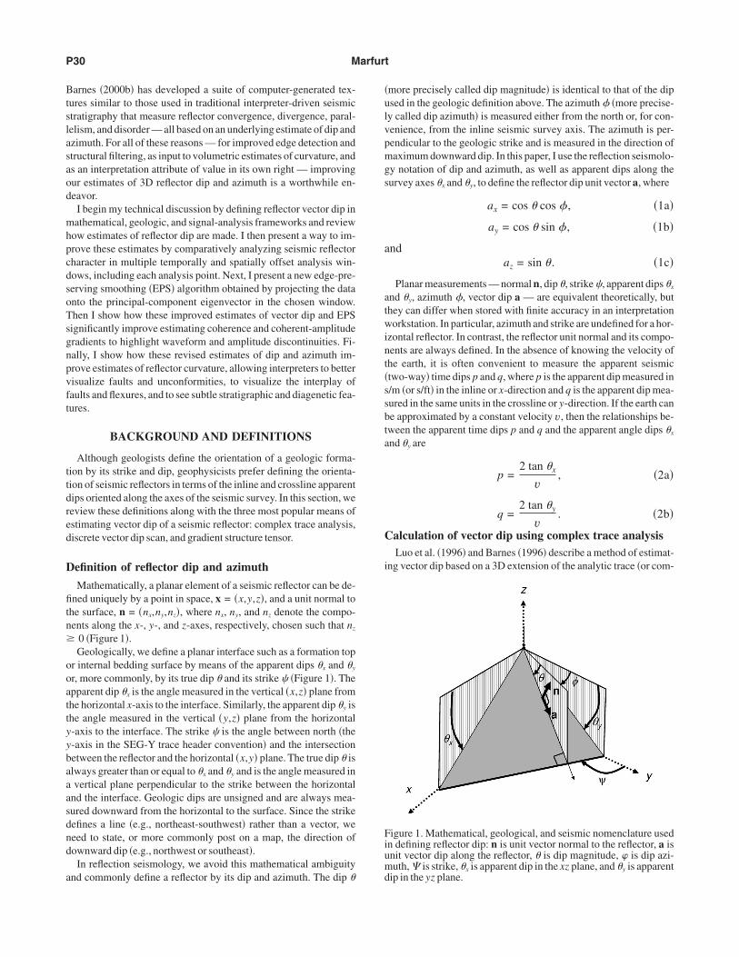
Mathematically, a planar element of a seismic reflector can be de-ned uniquely by a point in space, x = �x,y,z�, and a unit normal to

he surface, n = �nx,ny,nz�, where nx, ny, and nz denote the compo-ents along the x-, y-, and z-axes, respectively, chosen such that nz

0 �Figure 1�.Geologically, we define a planar interface such as a formation top

r internal bedding surface by means of the apparent dips �x and �y

r, more commonly, by its true dip � and its strike � �Figure 1�. Thepparent dip �x is the angle measured in the vertical �x,z� plane fromhe horizontal x-axis to the interface. Similarly, the apparent dip �y ishe angle measured in the vertical �y,z� plane from the horizontal-axis to the interface. The strike � is the angle between north �the-axis in the SEG-Y trace header convention� and the intersectionetween the reflector and the horizontal �x,y� plane. The true dip � islways greater than or equal to �x and �y and is the angle measured invertical plane perpendicular to the strike between the horizontal

nd the interface. Geologic dips are unsigned and are always mea-ured downward from the horizontal to the surface. Since the strikeefines a line �e.g., northeast-southwest� rather than a vector, weeed to state, or more commonly post on a map, the direction ofownward dip �e.g., northwest or southeast�.

In reflection seismology, we avoid this mathematical ambiguitynd commonly define a reflector by its dip and azimuth. The dip �

more precisely called dip magnitude� is identical to that of the dipsed in the geologic definition above. The azimuth � �more precise-y called dip azimuth� is measured either from the north or, for con-enience, from the inline seismic survey axis. The azimuth is per-endicular to the geologic strike and is measured in the direction ofaximum downward dip. In this paper, I use the reflection seismolo-

y notation of dip and azimuth, as well as apparent dips along theurvey axes �x and �y, to define the reflector dip unit vector a, where

ax = cos � cos � , �1a�

ay = cos � sin � , �1b�

ndaz = sin � . �1c�

Planar measurements — normal n, dip �, strike �, apparent dips �x

nd �y, azimuth �, vector dip a — are equivalent theoretically, buthey can differ when stored with finite accuracy in an interpretationorkstation. In particular, azimuth and strike are undefined for a hor-

zontal reflector. In contrast, the reflector unit normal and its compo-ents are always defined. In the absence of knowing the velocity ofhe earth, it is often convenient to measure the apparent seismictwo-way� time dips p and q, where p is the apparent dip measured in/m �or s/ft� in the inline or x-direction and q is the apparent dip mea-ured in the same units in the crossline or y-direction. If the earth cane approximated by a constant velocity v, then the relationships be-ween the apparent time dips p and q and the apparent angle dips �x

nd �y are

p =2 tan �x

v, �2a�

q =2 tan �y

v. �2b�

alculation of vector dip using complex trace analysisLuo et al. �1996� and Barnes �1996� describe a method of estimat-

ng vector dip based on a 3D extension of the analytic trace �or com-

igure 1. Mathematical, geological, and seismic nomenclature usedn defining reflector dip: n is unit vector normal to the reflector, a isnit vector dip along the reflector, � is dip magnitude, � is dip azi-uth, � is strike, �x is apparent dip in the xz plane, and �y is apparent

ip in the yz plane.

pw

wstveFi

a

a

dctftmtacdusnocTb

Tt

a

m

wi

F

Robust estimates of dip and azimuth P31

lex trace� attributes described by Taner et al. �1979�. They beginith Taner et al.’s �1979� instantaneous frequency �:

��t,x,y� =��

� t=

�

� tATAN2�uH,u� =

u�uH

� t− uH�u

� t

�u�2 + �uH�2 ,

�3�

here � denotes the instantaneous phase, u�t,x,y� denotes the inputeismic data, uH�t,x,y� denotes its Hilbert transform with respect toime t, and ATAN2 denotes the arctangent function whose outputaries between − and +. The derivatives of u and uH are obtainedither by using finite differences or via a Fourier transform, with theourier transform approach being particularly convenient since this

s the domain in which the Hilbert transform typically is calculated.The next step is to calculate the instantaneous wavenumbers kx

nd ky:

kx�t,x,y� =��

�x=

u�uH

�x− uH�u

�x

�u�2 + �uH�2

�4a�

nd

ky�t,x,y� =��

� y=

u�uH

� y− uH�u

� y

�u�2 + �uH�2 .

�4b�

The Hilbert transform can be calculated in anyirection we choose. It may appear to be moreonsistent to apply the Hilbert transform alonghe x-axis for computating kx and along the y-axisor ky. However, since there is only one Hilbertransform for the data, we estimate it along the

ore densely sampled vertical time axis, or-axis, where we encounter fewer artifacts fromliasing. For very large 3D input seismic dataubes, it is more convenient to estimate the spatialerivatives �u/�x, �uH/�x, �u/�y, and �uH/�y,sing either central differences or a relativelyhort Fourier transform. This circumvents theeed for keeping the entire data cube in memoryr, alternatively, for transposing the cube prior toalculating the derivatives given in equation 4.he instantaneous time dip �p,q� is then obtainedy calculating the ratio of kx and ky to �:

p = kx/� , �5a�

q = ky /� . �5b�

he azimuth �, measured from the y-axis, andrue time dip s are given by

� = ATAN2�q,p� �6a�

nd

s = �p2 + q2�1/2. �6b�

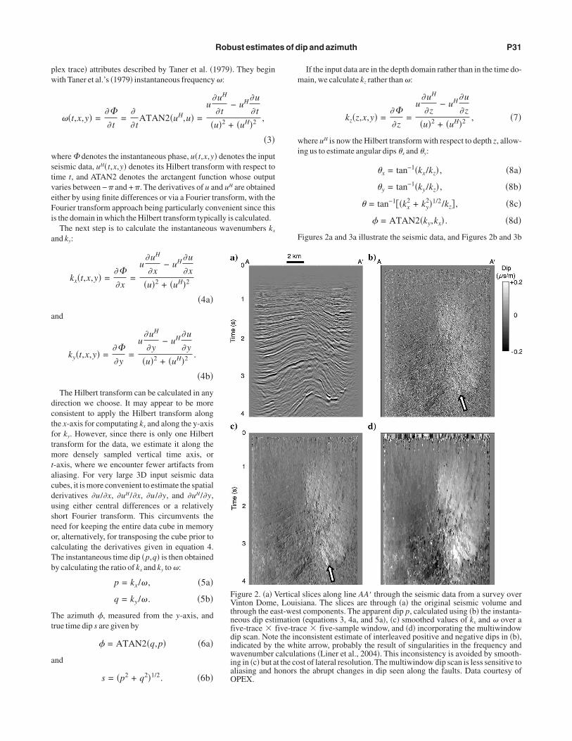
Figure 2. �a� VVinton Domethrough the eaneous dip estifive-trace fdip scan. Noteindicated by twavenumbering in �c� but aaliasing and hOPEX.

If the input data are in the depth domain rather than in the time do-ain, we calculate kz rather than �:

kz�z,x,y� =��

� z=

u�uH

� z− uH�u

� z

�u�2 + �uH�2 , �7�

here uH is now the Hilbert transform with respect to depth z, allow-ng us to estimate angular dips �x and �y:

�x = tan−1�kx/kz� , �8a�

�y = tan−1�ky /kz� , �8b�

� = tan−1��kx2 + ky

2�1/2/kz� , �8c�

� = ATAN2�ky,kx� . �8d�

igures 2a and 3a illustrate the seismic data, and Figures 2b and 3b

l slices along line AA� through the seismic data from a survey overiana. The slices are through �a� the original seismic volume andt components. The apparent dip p, calculated using �b� the instanta-�equations 3, 4a, and 5a�, �c� smoothed values of kx and � over a

ce five-sample window, and �d� incorporating the multiwindowconsistent estimate of interleaved positive and negative dips in �b�,ite arrow, probably the result of singularities in the frequency andtions �Liner et al., 2004�. This inconsistency is avoided by smooth-st of lateral resolution. The multiwindow dip scan is less sensitive tothe abrupt changes in dip seen along the faults. Data courtesy of

ertica, Louisst-wesmationive-trathe in

he whcalculat the coonors

ea

qebavttiEk

C

ni

s

wdJadpatsmc

Cg

sFgotvssltt

Ftnfdbsi

P32 Marfurt

xhibit the east-west component of instantaneous time dip p throughsalt dome near Vinton, Louisiana.Taner et al. �1979� warn that the estimate of instantaneous fre-

uency given by equation 3 suffers from singularities when reflectorvents interfere with each other. Indeed, such singularities form theasis of the SPICE algorithm �Liner et al., 2004�. To remedy this in-ccuracy, Taner et al. �1979� suggest replacing equation 3 with an en-elope-weighted average. Barnes �2000a� generalizes this concepto smoothing the calculation of �, kx, and ky over 25 or more adjacentraces prior to estimating dip and azimuth, thereby improving stabil-ty with only minor loss of lateral resolution �Figures 2c and 3c�.ven with such smoothing, the singularities in calculating �, kx, andy produce artifacts on the flanks of the dome.

alculation of vector dip by discrete scans

Marfurt et al. �1998� generalize Finn’s �1986� semblance scan-ing method to 3D data to generate a more robust means of estimat-ng reflector dip �Figure 4�:

��x,�y�

=

�k=KS

KE �� 1

J�j=1

J

u�k�t − pxj − qyj��2

+ � 1

J�j=1

J

uH�k�t − pxj − qyj��2�k=KS

KE � 1

J�j=1

J

�u�k�t − pxj − qyj��2 +1

J�j=1

J

�uH�k�t − pxj − qyj��2�9�

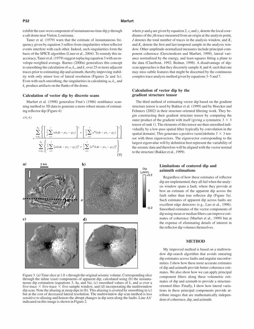
igure 3. �a� Time slice at 1.0 s through the original seismic volume.hrough the inline �east� components of apparent dip, calculated useous dip estimation �equations 3, 4a, and 5a�, �c� smoothed valueive-trace five-trace five-sample window, and �d� incorporatinip scan. Note the aliasing at steep dips in �b�. This aliasing is avertedut at the cost of decreased lateral resolution. The multiwindow dipensitive to aliasing and honors the abrupt changes in dip seen alongndicated on this image is shown in Figure 2.

here p and q are given by equation 2, xj and yj denote the local coor-inates of the jth trace measured from an origin at the analysis point,denotes the total number of traces in the analysis window, and Ks

nd Ke denote the first and last temporal sample in the analysis win-ow. Other amplitude-normalized measures include principal-com-onent coherence �Gersztenkorn and Marfurt, 1999�, lateral vari-nce normalized by the energy, and least-squares fitting a plane tohe data �Claerbout, 1992; Bednar, 1998�. A disadvantage of dip-can approaches is that they discretely sample �x and �y such that oneay miss subtle features that might be discerned by the continuous

omplex trace analysis method given by equations 3–5 and 7.

alculation of vector dip by theradient structure tensor

The third method of estimating vector dip based on the gradienttructure tensor is used by Bakker et al. �1999� and by Hoecker andehmers �2002� in their structure-oriented filtering work. They be-in constructing their gradient structure tensor by computing theuter product of the gradient with itself �giving a symmetric 3 3ensor of rank 1�. The elements of this tensor are then smoothed indi-idually by a low-pass spatial filter �typically by convolution in thepatial domain�. This generates a positive �semi�definite 3 3 ten-or with three eigenvectors. The eigenvector corresponding to theargest eigenvalue will by definition best represent the variability ofhe seismic data and therefore will be aligned with the vector normalo the structure �Bakker et al., 1999�.

Limitations of centered dip andazimuth estimations

Regardless of how these estimates of reflectordip are implemented, they all fail when the analy-sis window spans a fault, where they provide atbest an estimate of the apparent dip across thefault rather than true reflector dip �Figure 5a�.Such estimates of apparent dip across faults areexcellent edge detectors �e.g., Luo et al., 1996�.Smoothed estimates of the vector components ofdip using mean or median filters can improve esti-mates of coherence �Marfurt et al., 1999� but atthe expense of eliminating details of interest inthe reflector dip volumes themselves.

METHOD

My improved method is based on a multiwin-dow dip-search algorithm that avoids smearingdip estimates across faults and angular unconfor-mities. I show how these more accurate estimatesof dip and azimuth provide better coherence esti-mates. We also show how we can apply principalcomponent filters along these volumetric esti-mates of dip and azimuth to provide a structure-oriented filter. Finally, I show how lateral varia-tions in these principal components provide at-tribute images that are mathematically indepen-dent of coherence, dip, and azimuth.

ponding slicethe instanta-and � over amultiwindowoothing in �c�ethod is lesslts. Line AA�

Corresing �b�s of kx

g theby smscan mthe fau

R

sap

sl

ft

yeractw

wwr

ctmeuc�w

bu1toacpipt�ttsh

Fhv�deascldbct

FiCtta

Robust estimates of dip and azimuth P33

obust estimates of 3D vector dip

Equation 9 provides values of semblance on a grid of discretelyampled angle pairs ��x,�y�. I obtain an improved estimate of dip andzimuth by passing a 2D paraboloid through the nine discretely sam-led points neighboring the point having the maximum semblance:

s��x,�y� = �1�x2 + �2�x�y + �3�y

2 + �4�x + �5�y + �6,

�10�olving for the coefficients � j in a least-squares sense. I then calcu-ate an improved estimate of the vector dip by solving

� s��x,�y���x

= 2�1�̂x + �2�̂y + �4 = 0,

� s��x,�y���y

= �2�̂x + 2�3�̂y + �5 = 0 �11�

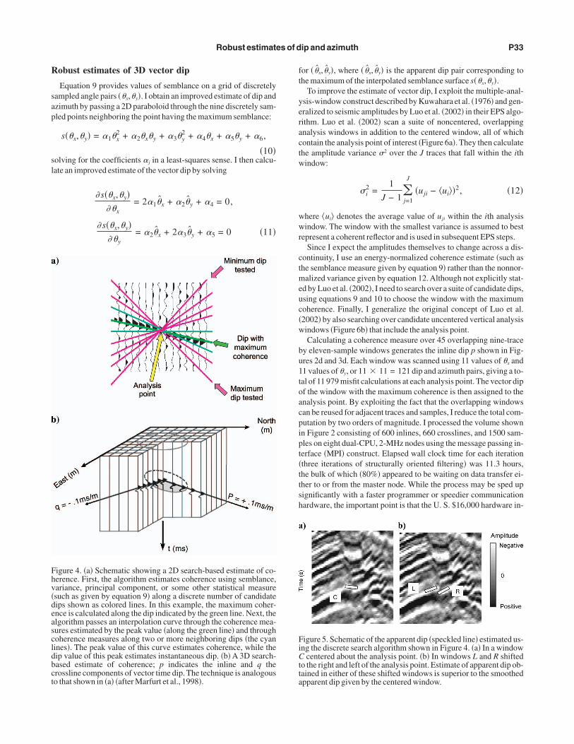
igure 4. �a� Schematic showing a 2D search-based estimate of co-erence. First, the algorithm estimates coherence using semblance,ariance, principal component, or some other statistical measuresuch as given by equation 9� along a discrete number of candidateips shown as colored lines. In this example, the maximum coher-nce is calculated along the dip indicated by the green line. Next, thelgorithm passes an interpolation curve through the coherence mea-ures estimated by the peak value �along the green line� and throughoherence measures along two or more neighboring dips �the cyanines�. The peak value of this curve estimates coherence, while theip value of this peak estimates instantaneous dip. �b� A 3D search-ased estimate of coherence; p indicates the inline and q therossline components of vector time dip. The technique is analogouso that shown in �a� �after Marfurt et al., 1998�.

or � �̂x, �̂y�, where � �̂x, �̂y� is the apparent dip pair corresponding tohe maximum of the interpolated semblance surface s��x,�y�.

To improve the estimate of vector dip, I exploit the multiple-anal-sis-window construct described by Kuwahara et al. �1976� and gen-ralized to seismic amplitudes by Luo et al. �2002� in their EPS algo-ithm. Luo et al. �2002� scan a suite of noncentered, overlappingnalysis windows in addition to the centered window, all of whichontain the analysis point of interest �Figure 6a�. They then calculatehe amplitude variance 2 over the J traces that fall within the ithindow:

i2 =

1

J − 1�j=1

J

�uji − ui��2, �12�

here ui� denotes the average value of uji within the ith analysisindow. The window with the smallest variance is assumed to best

epresent a coherent reflector and is used in subsequent EPS steps.Since I expect the amplitudes themselves to change across a dis-

ontinuity, I use an energy-normalized coherence estimate �such ashe semblance measure given by equation 9� rather than the nonnor-

alized variance given by equation 12. Although not explicitly stat-d by Luo et al. �2002�, I need to search over a suite of candidate dips,sing equations 9 and 10 to choose the window with the maximumoherence. Finally, I generalize the original concept of Luo et al.2002� by also searching over candidate uncentered vertical analysisindows �Figure 6b� that include the analysis point.Calculating a coherence measure over 45 overlapping nine-trace

y eleven-sample windows generates the inline dip p shown in Fig-res 2d and 3d. Each window was scanned using 11 values of �x and1 values of �y, or 11 11 = 121 dip and azimuth pairs, giving a to-al of 11 979 misfit calculations at each analysis point. The vector dipf the window with the maximum coherence is then assigned to thenalysis point. By exploiting the fact that the overlapping windowsan be reused for adjacent traces and samples, I reduce the total com-utation by two orders of magnitude. I processed the volume shownn Figure 2 consisting of 600 inlines, 660 crosslines, and 1500 sam-les on eight dual-CPU, 2-MHz nodes using the message passing in-erface �MPI� construct. Elapsed wall clock time for each iterationthree iterations of structurally oriented filtering� was 11.3 hours,he bulk of which �80%� appeared to be waiting on data transfer ei-her to or from the master node. While the process may be sped upignificantly with a faster programmer or speedier communicationardware, the important point is that the U. S. $16,000 hardware in-

igure 5. Schematic of the apparent dip �speckled line� estimated us-ng the discrete search algorithm shown in Figure 4. �a� In a window

centered about the analysis point. �b� In windows L and R shiftedo the right and left of the analysis point. Estimate of apparent dip ob-ained in either of these shifted windows is superior to the smoothedpparent dip given by the centered window.

ve

Ic

raty

wwwat

itetwuitmt

eddrmasfs

P

teiteacpeenttw

wld

Hd

ptcp

Ffrootseilisfiatgaap

P34 Marfurt

estment �2004 dollars� places such computation within the reach ofven the smallest technology providers.

mpact of robust reflector dip estimates onoherence estimates of reflector discontinuities

Bakker et al. �1999� note that the Kuwahara et al. �1976� algo-ithm can produce patchy images and suggest favoring the centerednalysis window when dealing with noisy data. I do so by modifyinghe semblance scent �or other coherence measure� at the centered anal-sis window to be

snewcent = ascent + b , �13�

here a � 1 and b � 1. Values of a = 1 and b = 0 reproduce Ku-ahara’s et al. �1976� original algorithm, while a value of b = 1.0ill force a centered, single-window algorithm. A value of a = 1.02

nd b = 0.1 works well for good-quality land data such as shown inhis paper.

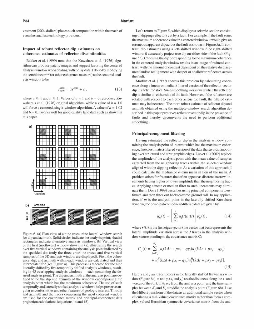
igure 6. �a� Plan view of a nine-trace, nine-lateral-window searchor dip and azimuth. Solid circles indicate the analysis point; shadedectangles indicate alternative analysis windows. �b� Vertical viewf the first �northwest� window shown in �a�, illustrating the searchver five vertical windows containing the analysis point indicated byhe speckled dot �only the three crossline traces and five verticalamples of the 3D analysis window are displayed�. First, the coher-nce, dip, and azimuth within each window are calculated and thennterpolated for �see Figure 4�. This process is repeated for the nineaterally shifted by five temporally shifted analysis windows, result-ng in 45 overlapping analysis windows — each containing the de-ired analysis point. The dip and azimuth at the analysis point are de-ned to be the dip and azimuth of the window encompassing thenalysis point which has the maximum coherence. The use of suchemporally and laterally shifted analysis windows helps preserve an-ular unconformities and other features of geologic interest. This dipnd azimuth and the traces comprising the most coherent windowre used for the covariance matrix and principal-component data

rojection calculations �equations 14 and 15�.

Let’s return to Figure 5, which displays a seismic section consist-ng of dipping reflectors cut by a fault. For a sample in the fault zone,he maximum coherence value in a centered window c would give anrroneous apparent dip across the fault as shown in Figure 5a. In con-rast, dip estimates using a left-shifted window L or right-shiftedindow R accurately project true dip on either side of the fault �Fig-re 5b�. Choosing the dip corresponding to the maximum coherencen the centered analysis window results in an image of reduced con-rast, with the amount of contrast dependent on the relative displace-

ent and/or realignment with deeper or shallower reflectors acrosshe fault.

Marfurt et al. �1999� address this problem by calculating coher-nce along a �mean or median� filtered version of the reflector vectorip in each time slice. Such smoothing works well when the reflectorip is similar on either side of the fault. However, if the reflectors areotated with respect to each other across the fault, the filtered esti-ate may be incorrect. The more robust estimate of reflector dip and

zimuth obtained using the multiple-window search algorithm de-cribed in this paper preserves reflector vector dip in the presence ofaults and thereby circumvents the need to perform additionalmoothing.

rincipal-component filtering

Having estimated the reflector dip in the analysis window con-aining the analysis point of interest which has the maximum coher-nce, I next estimate a filtered version of the data that avoids smooth-ng over structural and stratigraphic edges. Luo et al. �2002� replacehe amplitude of the analysis point with the mean value of samplesxtracted from the neighboring traces within the selected windowligned with the dipping reflector. As a variation of this approach, Iould calculate the median or �-trim mean in lieu of the mean. Aroblem arises for fractures that often appear as discrete, narrow lin-aments having higher or lower amplitude than the neighboring trac-s. Applying a mean or median filter to such lineaments may elimi-ate them. Done �1999� describes using principal components to es-imate and then filter out backscattered ground roll. In my applica-ion, if m is the analysis point in the laterally shifted Kuwaharaindow, the principal-component-filtered data are given by

um1 �t� = ��

j=1

J

uj�t�v j1�t��vm

1 �t� , �14�

here v1�t� is the first eigenvector �the vector that best represents theateral amplitude variation across the J traces in the analysis win-ow� corresponding to the covariance matrix C:

Cij�t� = �k=Ks

Ke

�ui�k�t + pxi − qyi�uj�k�t + pxj − qyj�

+ uiH�k�t + pxi − qyi�uj

H�k�t + pxj − qyj�� .

�15�

ere, i and j are trace indices in the laterally shifted Kuwahara win-ow �Figure 6a�, xi and yi �xj and yj� are the distances along the x- and

y-axes of the ith �jth� trace from the analysis point, and the time sam-les between Ks and Ke straddle the analysis point �Figure 6b�. I usehe Hilbert transform of the data as an additional sample vector whenalculating a real-valued covariance matrix rather than form a com-lex-valued Hermitian symmetric covariance matrix from the ana-

letscyijfedpy

cfijflfnmssttrsvctlefdswFtpIsf

Rp

dtdpdttksdsvt

aFshmflrp

C

vp

Robust estimates of dip and azimuth P35

ytic trace. Using the data and its Hilbert transform avoids unstablestimates of the covariance matrix for small vertical windows cen-ered about a trace zero crossing. Using a complex-valued Hermitianymmetric covariance matrix �and corresponding complex principalomponents� provides some extra, uncontrolled phase rotation be-ond that provided by the dip search and interpolation, and it resultsn images that have somewhat lower lateral resolution and noise re-ection. The covariance matrix calculation given by equation 15 dif-ers from that used by Gersztenkorn and Marfurt �1999� and Marfurtt al. �1999� in that I use the Hilbert transform of the input data in ad-ition to the input data itself and that, in general, the window is tem-orally and laterally shifted from rather than centered about the anal-sis point.

The behavior of Luo et al.’s �2002� EPS filter and the principal-omponent projection given by equation 14 are quite different. Bothlters suppress random noise. Both filters also re-

ect coherent noise cutting across the strongest re-ector in the window, such as backscattered sur-ace waves. Unfortunately, they can also elimi-ate desirable crosscutting signals, such as mis-igrated fault-plane reflections. Luo et al. �2002�

how how the edge-preserving mean filter canuppress the acquisition footprint. If the acquisi-ion footprint comes from leakage of side-scat-ered noise, then the principal component filtereduces the footprint better. However, the acqui-ition footprint can also be a function of signalariability from differences in fold, source-re-eiver offset, and source-receiver azimuth be-ween adjacent bins. Such differences are particu-arly sensitive to errors in velocity-induced NMOrrors �Hill et al., 1999�. In this case where theootprint pattern is slowly varying in the verticalirection, the principal-component filter will pre-erve and even enhance the acquisition footprint,hile a mean or median filter will suppress it.ractures that are nearly vertical are nearly indis-

inguishable from this kind of acquisition foot-rint. Since I am interested in mapping fractures,use the principal-component filter and accept

ome image contamination from the acquisitionootprint.

ecursive application ofrincipal-component filtering

Once an edge-preserving filtered version of theata is generated, I can use it recursively as inputo a second analysis, where I recalculate vectorip, coherence, amplitude gradients, and a secondass of filtering, if desired. For particularly noisyata, such as land data, we can greatly acceleratehe interpretation process by using autopickers onhe smoothed data, as recommended by Hoec-er and Fehmers �2002�. These picks on themoothed data can then be transferred to the moreifficult-to-pick original data by snapping themoothed picks to peaks or troughs of previousersions of the data. I plot the data correspondingo line AA� in Figure 2a on the face of a folded im-

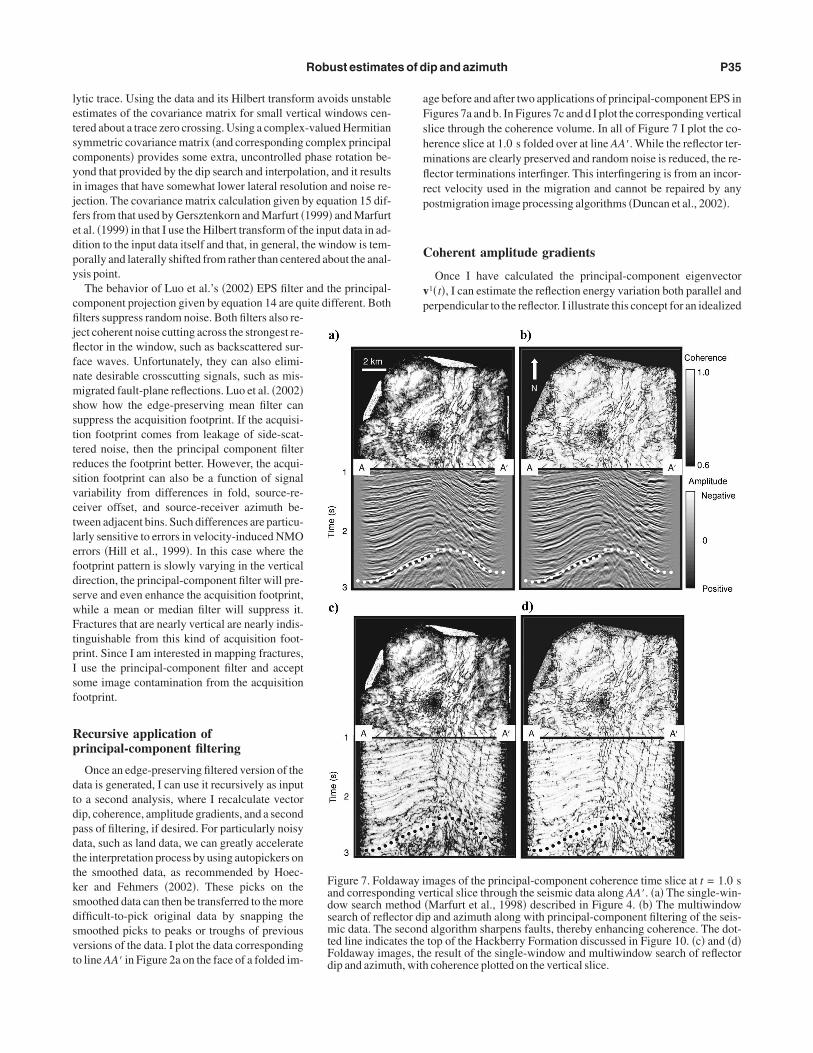
Figure 7. Foldand correspondow search msearch of reflemic data. Theted line indicaFoldaway imadip and azimu

ge before and after two applications of principal-component EPS inigures 7a and b. In Figures 7c and d I plot the corresponding verticallice through the coherence volume. In all of Figure 7 I plot the co-erence slice at 1.0 s folded over at line AA�. While the reflector ter-inations are clearly preserved and random noise is reduced, the re-ector terminations interfinger. This interfingering is from an incor-ect velocity used in the migration and cannot be repaired by anyostmigration image processing algorithms �Duncan et al., 2002�.

oherent amplitude gradients

Once I have calculated the principal-component eigenvector1�t�, I can estimate the reflection energy variation both parallel anderpendicular to the reflector. I illustrate this concept for an idealized

mages of the principal-component coherence time slice at t = 1.0 sertical slice through the seismic data along AA�. �a� The single-win-�Marfurt et al., 1998� described in Figure 4. �b� The multiwindowp and azimuth along with principal-component filtering of the seis-algorithm sharpens faults, thereby enhancing coherence. The dot-

top of the Hackberry Formation discussed in Figure 10. �c� and �d�e result of the single-window and multiwindow search of reflectorcoherence plotted on the vertical slice.

away iding vethodctor disecondtes theges, thth, with

2ciwatg

dttcct

ortcgtun

acntgvtglagevr

tfteadw

w

Ffilcfowptcthe analysis window in step 3.

Fne�elif

P36 Marfurt

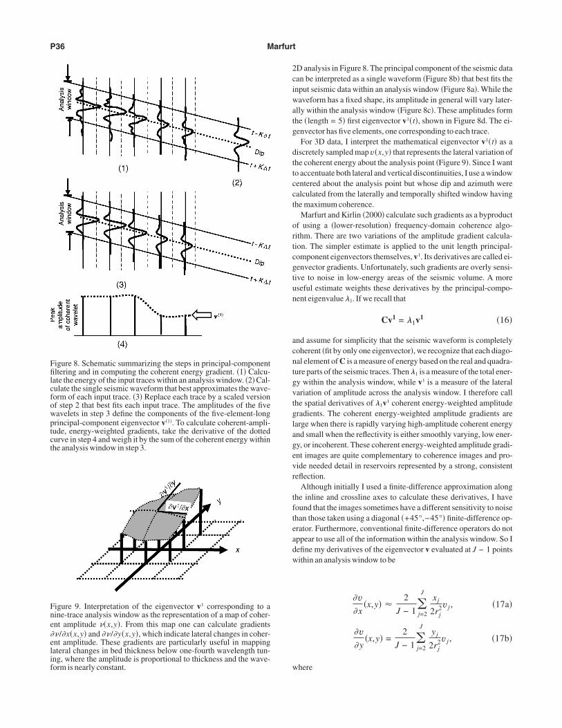
D analysis in Figure 8. The principal component of the seismic dataan be interpreted as a single waveform �Figure 8b� that best fits thenput seismic data within an analysis window �Figure 8a�. While theaveform has a fixed shape, its amplitude in general will vary later-

lly within the analysis window �Figure 8c�. These amplitudes formhe �length = 5� first eigenvector v1�t�, shown in Figure 8d. The ei-envector has five elements, one corresponding to each trace.

For 3D data, I interpret the mathematical eigenvector v1�t� as aiscretely sampled map v�x,y� that represents the lateral variation ofhe coherent energy about the analysis point �Figure 9�. Since I wanto accentuate both lateral and vertical discontinuities, I use a windowentered about the analysis point but whose dip and azimuth werealculated from the laterally and temporally shifted window havinghe maximum coherence.

Marfurt and Kirlin �2000� calculate such gradients as a byproductf using a �lower-resolution� frequency-domain coherence algo-ithm. There are two variations of the amplitude gradient calcula-ion. The simpler estimate is applied to the unit length principal-omponent eigenvectors themselves, v1. Its derivatives are called ei-envector gradients. Unfortunately, such gradients are overly sensi-ive to noise in low-energy areas of the seismic volume. A moreseful estimate weights these derivatives by the principal-compo-ent eigenvalue �1. If we recall that

Cv1 = �1v1 �16�

nd assume for simplicity that the seismic waveform is completelyoherent �fit by only one eigenvector�, we recognize that each diago-al element of C is a measure of energy based on the real and quadra-ure parts of the seismic traces. Then �1 is a measure of the total ener-y within the analysis window, while v1 is a measure of the lateralariation of amplitude across the analysis window. I therefore callhe spatial derivatives of �1v1 coherent energy-weighted amplituderadients. The coherent energy-weighted amplitude gradients arearge when there is rapidly varying high-amplitude coherent energynd small when the reflectivity is either smoothly varying, low ener-y, or incoherent. These coherent energy-weighted amplitude gradi-nt images are quite complementary to coherence images and pro-ide needed detail in reservoirs represented by a strong, consistenteflection.

Although initially I used a finite-difference approximation alonghe inline and crossline axes to calculate these derivatives, I haveound that the images sometimes have a different sensitivity to noisehan those taken using a diagonal �+45°,−45°� finite-difference op-rator. Furthermore, conventional finite-difference operators do notppear to use all of the information within the analysis window. So Iefine my derivatives of the eigenvector v evaluated at J − 1 pointsithin an analysis window to be

�v�x

�x,y� �2

J − 1�j=2

Jxj

2rj2v j , �17a�

�v� y

�x,y� =2

J − 1�j=2

Jyj

2rj2v j , �17b�

here

igure 8. Schematic summarizing the steps in principal-componentltering and in computing the coherent energy gradient. �1� Calcu-

ate the energy of the input traces within an analysis window. �2� Cal-ulate the single seismic waveform that best approximates the wave-orm of each input trace. �3� Replace each trace by a scaled versionf step 2 that best fits each input trace. The amplitudes of the fiveavelets in step 3 define the components of the five-element-longrincipal-component eigenvector v�1�. To calculate coherent-ampli-ude, energy-weighted gradients, take the derivative of the dottedurve in step 4 and weigh it by the sum of the coherent energy within

igure 9. Interpretation of the eigenvector v1 corresponding to aine-trace analysis window as the representation of a map of coher-nt amplitude ��x,y�. From this map one can calculate gradients�/�x�x,y� and ��/�y�x,y�, which indicate lateral changes in coher-nt amplitude. These gradients are particularly useful in mappingateral changes in bed thickness below one-fourth wavelength tun-ng, where the amplitude is proportional to thickness and the wave-orm is nearly constant.

Fttbcaw

Fu�c

Robust estimates of dip and azimuth P37

rj = �xj2 + yj

2�1/2. �17c�

The analysis point at the center of the window isomitted from the calculation. Inspection of theseformulas shows that they can be interpreted as anunweighted average of x- and y-components ofdirectional derivatives obtained by pairs of pointsstraddling the analysis point in the analysis win-dow.

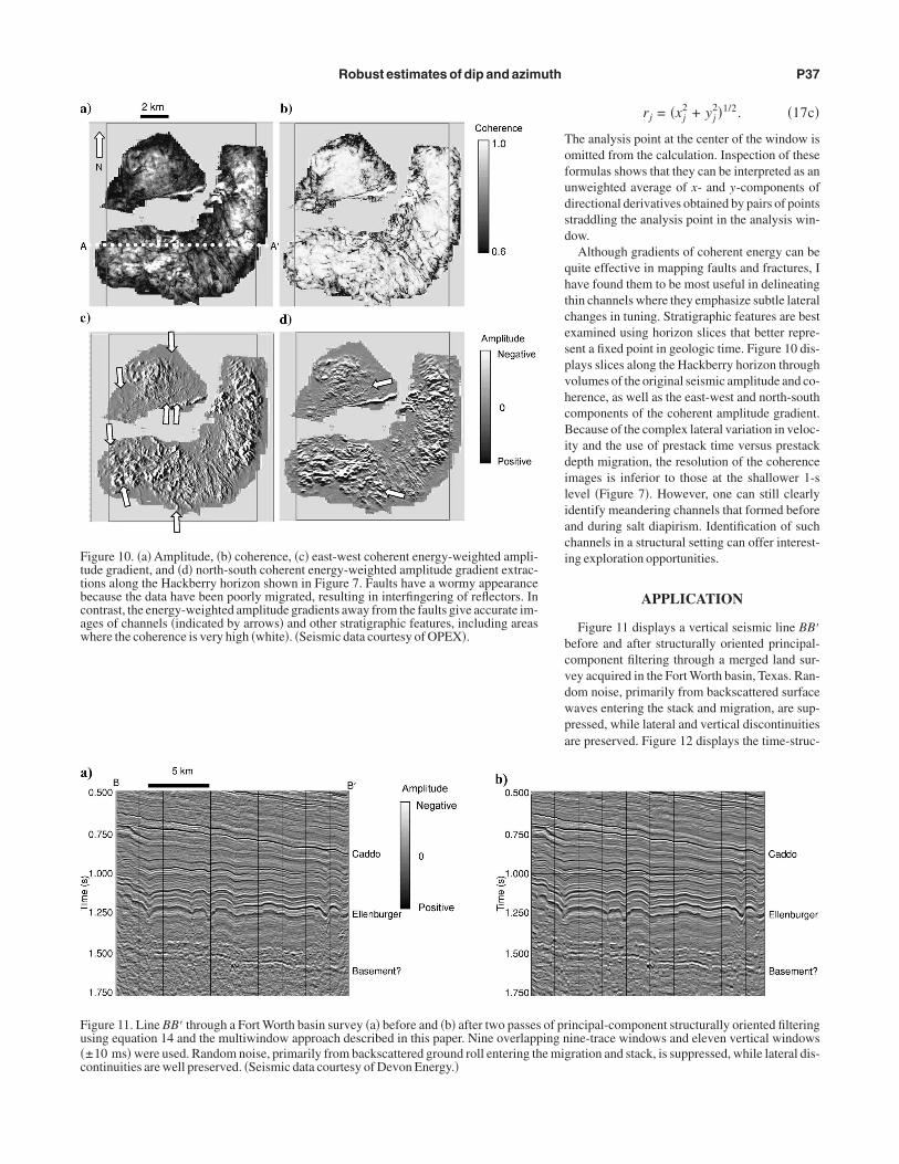
Although gradients of coherent energy can bequite effective in mapping faults and fractures, Ihave found them to be most useful in delineatingthin channels where they emphasize subtle lateralchanges in tuning. Stratigraphic features are bestexamined using horizon slices that better repre-sent a fixed point in geologic time. Figure 10 dis-plays slices along the Hackberry horizon throughvolumes of the original seismic amplitude and co-herence, as well as the east-west and north-southcomponents of the coherent amplitude gradient.Because of the complex lateral variation in veloc-ity and the use of prestack time versus prestackdepth migration, the resolution of the coherenceimages is inferior to those at the shallower 1-slevel �Figure 7�. However, one can still clearlyidentify meandering channels that formed beforeand during salt diapirism. Identification of suchchannels in a structural setting can offer interest-ing exploration opportunities.

APPLICATION

Figure 11 displays a vertical seismic line BB�before and after structurally oriented principal-component filtering through a merged land sur-vey acquired in the Fort Worth basin, Texas. Ran-dom noise, primarily from backscattered surfacewaves entering the stack and migration, are sup-pressed, while lateral and vertical discontinuitiesare preserved. Figure 12 displays the time-struc-

ighted ampli-dient extrac-y appearancereflectors. Inaccurate im-

cluding areas

ter two passes of principal-component structurally oriented filteringNine overlapping nine-trace windows and eleven vertical windowsoll entering the migration and stack, is suppressed, while lateral dis-

igure 10. �a� Amplitude, �b� coherence, �c� east-west coherent energy-weude gradient, and �d� north-south coherent energy-weighted amplitude graions along the Hackberry horizon shown in Figure 7. Faults have a wormecause the data have been poorly migrated, resulting in interfingering ofontrast, the energy-weighted amplitude gradients away from the faults giveges of channels �indicated by arrows� and other stratigraphic features, inhere the coherence is very high �white�. �Seismic data courtesy of OPEX�.

igure 11. Line BB� through a Fort Worth basin survey �a� before and �b� afsing equation 14 and the multiwindow approach described in this paper.±10 ms� were used. Random noise, primarily from backscattered ground rontinuities are well preserved. �Seismic data courtesy of Devon Energy.�

tClf1f

wml

Btio

th

vtTfpesanmTtvbto

Frddsdr

Ftttmvpw

P38 Marfurt

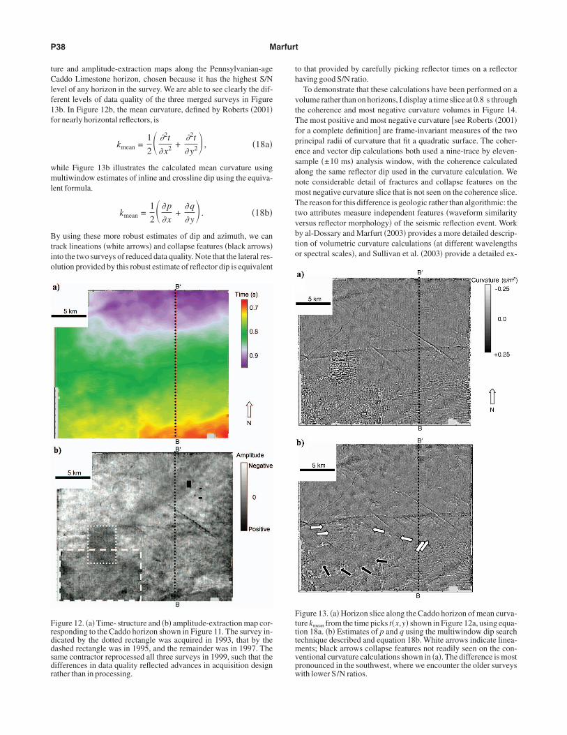
ure and amplitude-extraction maps along the Pennsylvanian-ageaddo Limestone horizon, chosen because it has the highest S/N

evel of any horizon in the survey. We are able to see clearly the dif-erent levels of data quality of the three merged surveys in Figure3b. In Figure 12b, the mean curvature, defined by Roberts �2001�or nearly horizontal reflectors, is

kmean =1

2 �2t

�x2 +�2t

� y2� , �18a�

hile Figure 13b illustrates the calculated mean curvature usingultiwindow estimates of inline and crossline dip using the equiva-

ent formula.

kmean =1

2 � p

�x+

�q

� y� . �18b�

y using these more robust estimates of dip and azimuth, we canrack lineations �white arrows� and collapse features �black arrows�nto the two surveys of reduced data quality. Note that the lateral res-lution provided by this robust estimate of reflector dip is equivalent

igure 12. �a� Time- structure and �b� amplitude-extraction map cor-esponding to the Caddo horizon shown in Figure 11. The survey in-icated by the dotted rectangle was acquired in 1993, that by theashed rectangle was in 1995, and the remainder was in 1997. Theame contractor reprocessed all three surveys in 1999, such that theifferences in data quality reflected advances in acquisition designather than in processing.

o that provided by carefully picking reflector times on a reflectoraving good S/N ratio.

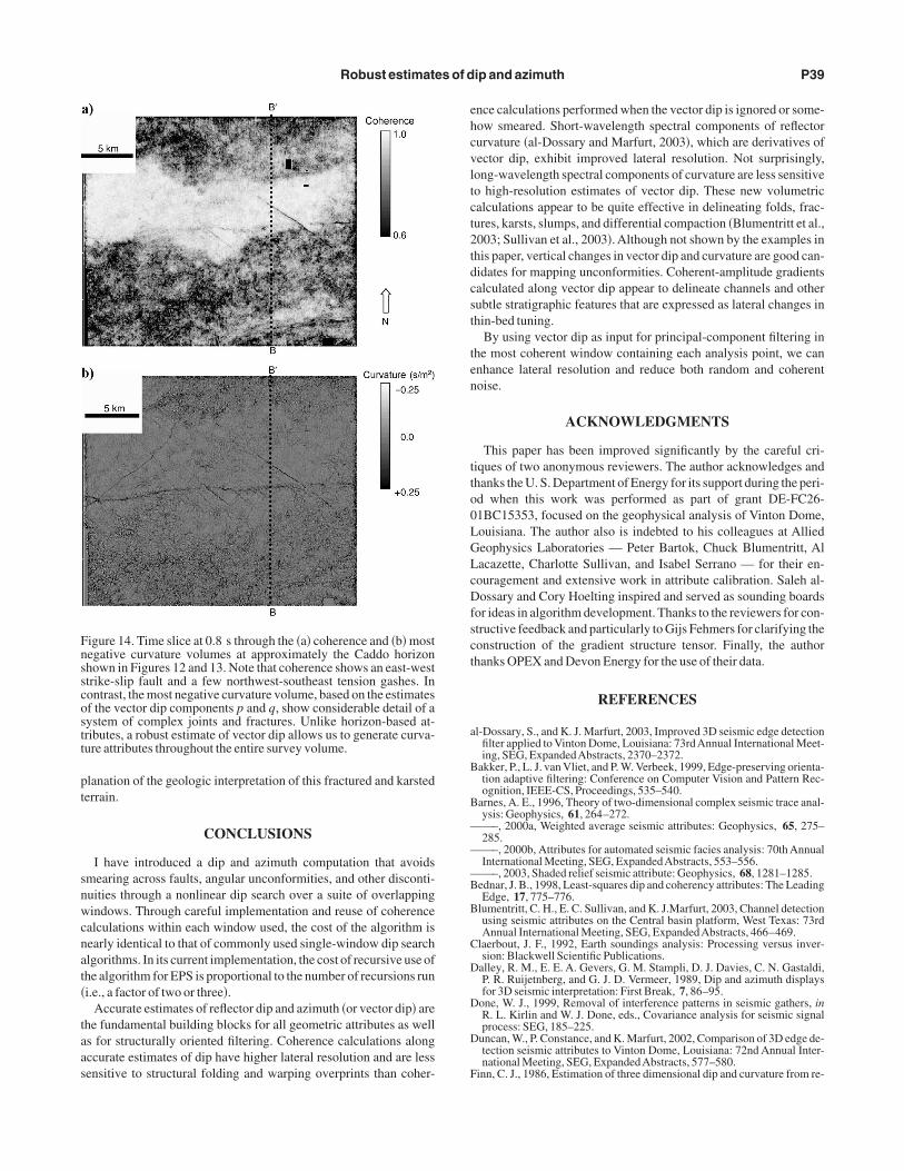
To demonstrate that these calculations have been performed on aolume rather than on horizons, I display a time slice at 0.8 s throughhe coherence and most negative curvature volumes in Figure 14.he most positive and most negative curvature �see Roberts �2001�

or a complete definition� are frame-invariant measures of the tworincipal radii of curvature that fit a quadratic surface. The coher-nce and vector dip calculations both used a nine-trace by eleven-ample �±10 ms� analysis window, with the coherence calculatedlong the same reflector dip used in the curvature calculation. Weote considerable detail of fractures and collapse features on theost negative curvature slice that is not seen on the coherence slice.he reason for this difference is geologic rather than algorithmic: the

wo attributes measure independent features �waveform similarityersus reflector morphology� of the seismic reflection event. Worky al-Dossary and Marfurt �2003� provides a more detailed descrip-ion of volumetric curvature calculations �at different wavelengthsr spectral scales�, and Sullivan et al. �2003� provide a detailed ex-

igure 13. �a� Horizon slice along the Caddo horizon of mean curva-ure kmean from the time picks t�x,y� shown in Figure 12a, using equa-ion 18a. �b� Estimates of p and q using the multiwindow dip searchechnique described and equation 18b. White arrows indicate linea-

ents; black arrows collapse features not readily seen on the con-entional curvature calculations shown in �a�. The difference is mostronounced in the southwest, where we encounter the older surveysith lower S/N ratios.

pt

snwcnat�

taas

ehcvltct2tdcst

ten

tto0LGLcDfsct

a

B

B

—

—

—B

B

C

D

D

D

F

Fnsscostt

Robust estimates of dip and azimuth P39

lanation of the geologic interpretation of this fractured and karstederrain.

CONCLUSIONS

I have introduced a dip and azimuth computation that avoidsmearing across faults, angular unconformities, and other disconti-uities through a nonlinear dip search over a suite of overlappingindows. Through careful implementation and reuse of coherence

alculations within each window used, the cost of the algorithm isearly identical to that of commonly used single-window dip searchlgorithms. In its current implementation, the cost of recursive use ofhe algorithm for EPS is proportional to the number of recursions runi.e., a factor of two or three�.

Accurate estimates of reflector dip and azimuth �or vector dip� arehe fundamental building blocks for all geometric attributes as wells for structurally oriented filtering. Coherence calculations alongccurate estimates of dip have higher lateral resolution and are lessensitive to structural folding and warping overprints than coher-

igure 14. Time slice at 0.8 s through the �a� coherence and �b� mostegative curvature volumes at approximately the Caddo horizonhown in Figures 12 and 13. Note that coherence shows an east-westtrike-slip fault and a few northwest-southeast tension gashes. Inontrast, the most negative curvature volume, based on the estimatesf the vector dip components p and q, show considerable detail of aystem of complex joints and fractures. Unlike horizon-based at-ributes, a robust estimate of vector dip allows us to generate curva-ure attributes throughout the entire survey volume.

nce calculations performed when the vector dip is ignored or some-ow smeared. Short-wavelength spectral components of reflectorurvature �al-Dossary and Marfurt, 2003�, which are derivatives ofector dip, exhibit improved lateral resolution. Not surprisingly,ong-wavelength spectral components of curvature are less sensitiveo high-resolution estimates of vector dip. These new volumetricalculations appear to be quite effective in delineating folds, frac-ures, karsts, slumps, and differential compaction �Blumentritt et al.,003; Sullivan et al., 2003�. Although not shown by the examples inhis paper, vertical changes in vector dip and curvature are good can-idates for mapping unconformities. Coherent-amplitude gradientsalculated along vector dip appear to delineate channels and otherubtle stratigraphic features that are expressed as lateral changes inhin-bed tuning.

By using vector dip as input for principal-component filtering inhe most coherent window containing each analysis point, we cannhance lateral resolution and reduce both random and coherentoise.

ACKNOWLEDGMENTS

This paper has been improved significantly by the careful cri-iques of two anonymous reviewers. The author acknowledges andhanks the U. S. Department of Energy for its support during the peri-d when this work was performed as part of grant DE-FC26-1BC15353, focused on the geophysical analysis of Vinton Dome,ouisiana. The author also is indebted to his colleagues at Alliedeophysics Laboratories — Peter Bartok, Chuck Blumentritt, Alacazette, Charlotte Sullivan, and Isabel Serrano — for their en-ouragement and extensive work in attribute calibration. Saleh al-ossary and Cory Hoelting inspired and served as sounding boards

or ideas in algorithm development. Thanks to the reviewers for con-tructive feedback and particularly to Gijs Fehmers for clarifying theonstruction of the gradient structure tensor. Finally, the authorhanks OPEX and Devon Energy for the use of their data.

REFERENCES

l-Dossary, S., and K. J. Marfurt, 2003, Improved 3D seismic edge detectionfilter applied to Vinton Dome, Louisiana: 73rdAnnual International Meet-ing, SEG, ExpandedAbstracts, 2370–2372.

akker, P., L. J. van Vliet, and P. W. Verbeek, 1999, Edge-preserving orienta-tion adaptive filtering: Conference on Computer Vision and Pattern Rec-ognition, IEEE-CS, Proceedings, 535–540.

arnes, A. E., 1996, Theory of two-dimensional complex seismic trace anal-ysis: Geophysics, 61, 264–272.—–, 2000a, Weighted average seismic attributes: Geophysics, 65, 275–285.—–, 2000b, Attributes for automated seismic facies analysis: 70th AnnualInternational Meeting, SEG, ExpandedAbstracts, 553–556.—–, 2003, Shaded relief seismic attribute: Geophysics, 68, 1281–1285.

ednar, J. B., 1998, Least-squares dip and coherency attributes: The LeadingEdge, 17, 775–776.

lumentritt, C. H., E. C. Sullivan, and K. J.Marfurt, 2003, Channel detectionusing seismic attributes on the Central basin platform, West Texas: 73rdAnnual International Meeting, SEG, ExpandedAbstracts, 466–469.

laerbout, J. F., 1992, Earth soundings analysis: Processing versus inver-sion: Blackwell Scientific Publications.

alley, R. M., E. E. A. Gevers, G. M. Stampli, D. J. Davies, C. N. Gastaldi,P. R. Ruijetnberg, and G. J. D. Vermeer, 1989, Dip and azimuth displaysfor 3D seismic interpretation: First Break, 7, 86–95.

one, W. J., 1999, Removal of interference patterns in seismic gathers, inR. L. Kirlin and W. J. Done, eds., Covariance analysis for seismic signalprocess: SEG, 185–225.

uncan, W., P. Constance, and K. Marfurt, 2002, Comparison of 3D edge de-tection seismic attributes to Vinton Dome, Louisiana: 72nd Annual Inter-national Meeting, SEG, ExpandedAbstracts, 577–580.

inn, C. J., 1986, Estimation of three dimensional dip and curvature from re-

G

H

H

H

H

K

L

L

L

L

—

L

M

M

M

P

R

S

S

T

P40 Marfurt

flection seismic data: M.S. thesis, University of Texas atAustin.ersztenkorn, A., and K. J. Marfurt, 1999, Eigenstructure based coherencecomputations as an aid to 3D structural and stratigraphic mapping: Geo-physics, 64, 1468–1479.

art, B. S., R. Pearson, and G. C. Rawling, 2002, 3D seismic horizon-basedapproaches to fracture-swarm sweet spot definition in tight-gas reservoirs:The Leading Edge, 21, 28–35.

esthammer, J., and H. Fossen, 1997, The influence of seismic noise in struc-tural interpretation of seismic attribute maps: First Break, 15, 209–219.

ill, S., M. Shultz, and J. Brewer, 1999, Acquisition footprint and fold-of-stack plots: The Leading Edge, 18, 686–695.

oecker, C., and G. Fehmers, 2002, Fast structural interpretation with struc-ture-oriented filtering: The Leading Edge, 21, 238–243.

uwahara, M., K. Hachimura, S. Eiho, and M. Kinoshita, 1976, Digital pro-cessing of biomedical images: Plenum Press, 187–203.

in, M. I.-C., K. J. Marfurt, and O. Johnson, 2003, Mapping 3D multiat-tribute data into HLS color space — Applications to Vinton Dome, LA:73rd Annual International Meeting, SEG, Expanded Abstracts, 1728–1731.

iner, C., C.-F. Li, A. Gerztenkorn, and J. Smythe, 2004, SPICE: A new gen-eral seismic attribute: 72nd Annual International Meeting, SEG, Expand-edAbstracts, 433–436.

isle, R. J., 1994, Detection of zones of abnormal strains in structures usingGaussian curvature analysis: AAPG Bulletin, 79, 1811–1819.

uo, Y., S. al-Dossary, and M. Marhoon, 2001, Generalized Hilbert trans-form and its application in geophysics: 71stAnnual International Meeting,

SEG, ExpandedAbstracts, 1835–1838.—–, 2002, Edge-preserving smoothing and applications: The LeadingEdge, 21, 136–158.

uo, Y., W. G. Higgs, and W. S. Kowalik, 1996, Edge detection and strati-graphic analysis using 3D seismic data: 66th Annual International Meet-ing, SEG, ExpandedAbstracts, 324–327.arfurt, K. J., and R. L. Kirlin, 2000, 3D broadband estimates of reflector dipand amplitude: Geophysics, 65, 304–320.arfurt, K. J., R. L. Kirlin, S. H. Farmer, and M. S. Bahorich, 1998, 3D seis-mic attributes using a running window semblance-based algorithm: Geo-physics, 63, 1150–1165.arfurt, K. J., V. Sudhakar, A. Gersztenkorn, K. D. Crawford, and S. E. Nis-sen, 1999, Coherency calculations in the presence of structural dip:Geophysics 64, 104–111.

icou, C., and R. Utzmann, 1962, La coupe sismique vectorielle: Un pointésemi-automatique: Geophysical Prospecting, 4, 497–516.

oberts, A., 2001, Curvature attributes and their application to 3D interpret-ed horizons: First Break, 19, 85–100.

cheuer, T. E., and D. W. Oldenberg, 1988, Local phase velocity from com-plex seismic data: Geophysics, 53, 1503–1511.

ullivan, E. C., K. J. Marfurt, and M. Ammerman, 2003, Bottoms up karst:New 3D seismic attributes shed light on the Ellenberger �Ordovician� car-bonates in the Fort Worth basin �north Texas, USA�: 73rd Annual Interna-tional Meeting, SEG, ExpandedAbstracts, 482–485.

aner, M. T., F. Koehler, and R. E. Sheriff, 1979, Complex seismic trace anal-ysis: Geophysics, 44, 1041–1063.