Robust Energy Storage Scheduling for ImbalanceReduction of Strategically Formed Energy Balancing

Groups

Shantanu Chakrabortya,∗, Toshiya Okabea

aSmart Energy Research Laboratories, Central Research Laboratories, NEC Corporation,Japan.

Abstract

Imbalance (on-line energy gap between contracted supply and actual demand,and associated cost) reduction is going to be a crucial service for a Power Pro-ducer and Supplier (PPS) in the deregulated energy market. PPS requires for-ward market interactions to procure energy as precisely as possible in order toreduce imbalance energy. This paper presents, 1) (off-line) an effective demandaggregation based strategy for creating a number of balancing groups that leadsto higher predictability of group-wise aggregated demand, 2) (on-line) a robustenergy storage scheduling that minimizes the imbalance for a particular balanc-ing group considering the demand prediction uncertainty. The group formationis performed by a Probabilistic Programming approach using Bayesian MarkovChain Monte Carlo (MCMC) method after applied on the historical demandstatistics. Apart from the group formation, the aggregation strategy (with thehelp of Bayesian Inference) also clears out the upper-limit of the required stor-age capacity for a formed group, fraction of which is to be utilized in on-lineoperation. For on-line operation, a robust energy storage scheduling methodis proposed that minimizes expected imbalance energy and cost (a non-linearfunction of imbalance energy) while incorporating the demand uncertainty ofa particular group. The proposed methods are applied on the real apartmentbuildings’ demand data in Tokyo, Japan. Simulation results are presented toverify the effectiveness of the proposed methods.

Keywords: Robust Energy Storage Scheduling, Balancing Groups, StochasticOptimization, Mixed Integer Linear Programming, On-line ResourceScheduling, Bayesian Markov Chain Monte Carlo.

∗Corresponding authorEmail address: s-chakraborty@cp.jp.nec.com (Shantanu Chakraborty)

Preprint submitted to arxiv August 29, 2018

arX

iv:1

608.

0829

2v1

[cs

.SY

] 3

0 A

ug 2

016

1. Introduction

The number of Power Producer and Supplier (PPS) in the power and energymarket is increasing rapidly due to the liberalization in power market in Japan[1]. With the increase in market share of PPSs, the potential of demand-centricbusiness opportunity increases. As of 2014, the electricity market in Japan isdominated by regional monopolies, where 85% of the installed generating capac-ity is produced by 10 privately owned companies. However, the rising of PowerProducer and Supplier (PPS) (i.e. Electric Power Retailer) in the electricitymarket is inevitable due to the full-fledged deregulation [1] that will eventuallybreak the monopolies. PPPs face challenge while keeping the on-line supply anddemand matched with the highest precision, and thus reducing the imbalance(gap between contracted supply and demand) in demand side low-voltage net-work. In off-line, the PPS can intelligently group the customers to increase thedemand predictability of each group and procures volume of energy (utilizingday-ahead energy prediction). The procured energy refers as the supply con-tract for each group. Flexible power distribution as such is attainable throughDigital grid architecture [2]. In ideal world, the contracted supply matches withactual demand at each granular (typically, 30-minutes). However, due to theuncertainty in on-line energy consumption as well as energy supply, the gapbetween supply and demand is highly likely to occur. The current practice isto buy (in case of demand is higher than the supply) or sell (in case of supplyis higher than the demand) energy from/to Energy Imbalance Market (EIM)(EIM can be a part of Utility or be an independent body or the Utility itself,[3]). The EIM mitigates such mismatch between on-line supply and demand bytransacting necessary energy with the PPS. The involvement of EIM goes higherwith the increasing gap between the supply and the demand. The price settingof EIM, on the other hand, is significantly higher compared to the conventionalenergy tariff ([3], page 4). Therefore, the reduction of imbalance cost casts itselfas one of the important problems to tackle for demand side based energy serviceof PPS.

Two fundamental yet interconnected problems are, therefore, identified fora PPS, 1) strategic demand aggregation for balancing group creation, and 2)on-line imbalance energy and cost reduction for formed balancing groups. APPS serves multiple commercial settings (e.g. apartment buildings, commercialbuildings, shopping mall, factory, etc.). Therefore, it is essential for the PPSto effectively and strategically identify the customers’ demand based groupingfor energy balancing purpose, i.e. balancing group. Groupings as such are alsonecessary for service and price differentiations. In case of the imbalance energyreduction service, it is critically important for the PPS to define appropriatedemand aggregation criterion and demand aggregation strategy so that it caneffectively identify clusters of similar customers (e.g. buildings), the associ-ated aggregated demand with reduced variance and potential imbalance energybound. In this paper, we present a probabilistic programming [4] approach thatutilizes a Bayesian Markov Chain Monte Carlo (MCMC) sampling method [5][6] in order to form multiple balancing groups. Initially, a demand aggregation

2

criterion is identified as a statistical observation, then a probabilistic model ofthe observation is devised and finally posteriors of the model parameters aredetermined through Bayesian MCMC. The process is recursively conducted,which divides a parent observation into two based on the posterior analysis ofthe model parameters. Therefore, a divide-and-conquer approach is designed tosolve balancing group formation problem.

As for the on-line operation, the reduction of the group-wise imbalance costcan be realized by the effective on-line energy storage management; more par-ticularly, the on-line charge/discharge (CD) scheduling of energy storage. How-ever, since the imbalance energy tariff is non-linear to the imbalance energy,typical straight-forward method of CD scheduling leads to an inefficient solu-tion. Therefore, we present an efficient CD scheduling for multiple spatiallydistributed energy storages where the schedule is robust against demand pre-diction uncertainty. The robust scheduling method essentially minimizes theexpected imbalance energy and imbalance cost considering a number of demandprediction scenarios. Battery storage system is utilized as the energy storagesystem. The designed scheduling approach first performs a short-term demandprediction, then generates a number of statistical scenarios of the predicted de-mands utilizing a joint distribution of probability density function (PDF) of pre-diction error with the PDF of variability of preceding periods; and finally solvesa multi-objective optimization problem that decides the CD scheduling (withpower dispatch) of batteries while minimizing both imbalance energy and cost.The required aggregated battery power-rating information is drawn from theposterior distribution knowledge that had been conducted while forming groups.The problem in hand is non-linear due to the imbalance pricing scheme, storagedynamics and associated non-linear constraints. The optimization problem is,therefore, transformed into an equivalent Mixed Integer Linear Programming(MILP) problem [7] followed by an additional transformation to Mixed LogicalDynamical (MLD) System [8], and finally solved by a branch-and-cut linearsolver [9].

1.1. Related Works

Clustering has been a useful analytical and operational tool in energy do-main (e.g. energy market, [10]). Applications of clustering methods in high- andmedium-voltage power networks for large scale integration of customers havebeen reported in articles like [11] and [12]. In [11], a comprehensive overview ofclustering methods are presented and the necessity of these methods while iden-tifying effective customer grouping are highlighted (from the perspective of anEnergy Supplier). The supervised clustering algorithms (e.g. Hierarchical clus-tering, K-means, Fuzzy K-means) are discussed [12] that analyzes the similaritywithin customers. Meanwhile, at the low-voltage network, energy based cluster-ing for planning and operation (from the perspective of market operators suchas Distribution Network Operators, DNOs) is reported in [13]. In [13], house-hold smart-meter data are analyzed for demand variability and a finite mixturemodel based clustering algorithm is proposed that discovers a number of dis-tinctive behavior groups. Therefore, it is evident that clustering methods play

3

important roles for planning and operation of market operators such as energysuppliers, DNOs and PPSs. We employed a Bayesian inference coupled withMCMC method to determine the energy balancing groups based on a statisticaldemand measurement. The Bayesian MCMC is chosen over other clusteringmethods due to its advantages of accounting the uncertainty presented in themodels and parameters as well as its ability to present useful insights regard-ing the model (inferred from the posterior distribution of model’s parameters).For example, the applied Bayesian MCMC method provides an upper-bound ofrequired group-wise energy storage aggregated power-rating (and consequentlyenergy capacity rating).

For on-line operation, which requires fast solution, it has been widely ad-vised by the experts to deploy advanced mathematical optimization algorithmsthat accounts for system uncertainty and predictability of future states or con-ditions [14]. The working mechanism of the proposed CD scheduling method,therefore, aligns with that of Model Predictive Control (MPC), which measuresup to the aforementioned requirements. MPC (and its variants) has been anactive research area in the power system arena. In [15], an energy managementsystem for Microgrid operation considering PV, Diesel Generators, and energystorage is presented. A stochastic MPC for solving Unit Commitment withwind power is documented in [16]. Robust scheduling of resources is criticallyimportant when the optimization model is exposed to various uncertainties pre-sented in the model states. For example, in [17], a robust cost optimizationmethod is presented that essentially schedules of renewable energy generatorswith combined heat and power (CHP) generators considering the uncertaintyin net energy demand and electricity price. Another stream of research hasbeen conducted on stochastic MPC considering the uncertainty in the model.For example, in [18], a stochastic MPC is presented for efficient controlling inbuilding’s HVAC system while focusing on energy minimization. On the otherhand, MILP based mathematical optimization is the current industry trend ofoperation research oriented towards resource scheduling and optimization. Forinstance, in the arena of Unit Commitment (one of the important problemsin Power System Planning and Operation), MILP provides efficient, fast andscalable solutions [19] [20]. These outstanding researches create platform forapplying robust MILP based optimization algorithm, which minimizes the ex-pected imbalance energy and cost over a set predicted demand scenarios, as acore optimizer of the proposed on-line CD scheduling method.

2. Forming Energy Balancing Groups

An energy balancing group contains a number of customers1 sharing simi-larity in their demand profiles where their aggregated demand profile exhibitshigher predictability. It is, therefore, essential to identify appropriate criterion

1Being specific to this manuscript, the customers are the apartments buildings (or simplybuildings).

4

based on which such aggregation and group formation will be performed. Thefollowing is one such criterion.

2.0.1. Maximum Demand Standard Deviation of Periodic Demand

This measure is defined as the maximum of demand standard deviation(DSD), MDSD of a particular customer. The DSD tells how the demandof a particular period deviates from the average demand of that period over arange of sampling days. For example, if the demand is sampled over January(containing 31 days), the DSD of 10 AM is the statistical standard deviationover all the demands at 10AM accumulated in January. The MDSD is thusdefined as the following

MDSD = max {σt(Di(t))} . (1)

where t = 1, ..., N (N is the number of periods in a day, e.g. N = 48 for a day of30-minutes granularity) and i = 1, ..., ND (ND is the total number of samplingdays). MDSD is an absolute (demand) measure that stems from the in-perioddemand variations over different days.

From a PPS’s perspective, the customers that lower the accumulatedMDSDare desirable, since those customers have similarities in demand pattern as wellas higher predictability in their aggregated demand2. MDSDc is, therefore,identified as the demand aggregation criterion DACc, for a particular customerc. MDSD is considered to be an extremely important criterion since it can pro-vide insights regarding potential imbalance that might occur in real-time. Morespecifically, MDSD says about the worst deviation (from the average demand)that likely to occur over a particular day, consequently, the maximum powerrequired to nullify the deviation. As batteries are deployed to countermeasurethe imbalance, certain insights regarding the required battery power is essen-tial. Therefore, MDSD seems to be a better choice over other criteria as faras imbalance reduction is concerned. Other criteria, such as medians of dailyload factor, total periodical demand, daily average demand, etc. could also beutilized (either stand-alone or in combination) as DACc depending on the goalof the design. In this paper, therefore, we limit the DAC only to MDSD.

2.1. Demand Aggregation Strategy

The demand aggregation strategy performs a demand grouping scheme thatprovides several effective balancing groups of customers. The strategy first de-termines the DACs for all customers using their historical demand profiles. Thestrategy then applies a divide and conquer algorithm that recursively utilizesa Probabilistic Programming on the DACs. The Bayesian MCMC samplingmethod is chosen as the Probabilistic Programming. The Probabilistic Program-ming approach basically designs a probabilistic model for observing the DACs(referred as observation) by utilizing statistical knowledge regarding model pa-rameters (such as, when and how the observation changes with the arrival of new

2So called Laws of Large Numbers.

5

customer), represented by associated probability distributions and later utilizesBayesian inference to generate posterior distributions of the model parameters(by sampling through MCMC).

Figure 1: Flow-chart of a divide and conquer based group formation (demandaggregation strategy).

Figure 2: Flow-chart of the Bayesian MCMC sampling method generatingposterior distributions of the model parameters.

The process of Demand Aggregation Strategy (i.e. demand based energybalancing group formation) is depicted in Figure 1. In the flowchart, NC isnumber of individual customers. Note that, the method divides a group intotwo and recursively solves the sub-group formation problem. The output ofthe process is a list of group information where each item in the list representsthe range of the group (start and end). In detail, as depicted in Fig 1, thecustomers are organized in ascending order according to their DACs. The initialbalancing group contains all of the customers (i.e. a single group). The initialobservation contains the DAC values of all customers. The next step is to buildthe probabilistic model and use Bayesian MCMC sampling method to generateposterior distributions of model parameters. Fig 2 shows the flow-chart of thegroup partition process. Basically, the observation is where the model tryingto fit-in by varying the model parameters. At first the hyper-parameter (theparameter that controls the other parameters) α is determined. The parameterα (Eq. 2, where NO is number of observations) is set as the inverse of theexpected observations and is used to parameterize the prior distributions of λ1and λ2 (Eq. 3). What follows are the key features of the process.

1. Uniform distribution for the articulated customers3; parameter, τ (Eq. 4).

2. Exponential Distributions of DAC before and after the articulated cus-tomers; parameters, λ1 and λ2; which in turn parameterized by α (Eq3).

3. λ is formed deterministically by combining λ1 and λ2 where the mergingpoint is determined by distribution τ and customer identifier c (Eq. 5).

4. The DAC values are hypothesized by a Poisson Distribution4 with λ asexpected value (Eq. 6).

Figure 3: Model parameters and internal dependencies.

3The term “articulated customers” is defined as the customers whose DAC differs ‘signif-icantly’ with the same of preceding customers when the customers are ordered ascending-lyaccording to their DACs. In other words, an articulated customer defines the boundary of po-tential energy balancing groups. Every customer is equally likely to be an articulated customer(prior belief; before an observation of DAC is made). Therefore, the probability (parameterτ) of a particular customer to be an articulated customer is uniformly distributed over thenumber of customers

4The distribution of DAC is chosen to be a Poisson Distribution, since the DAC of acustomer is independent of each other and can be treated as a form of count data occurredin a discrete time event.

6

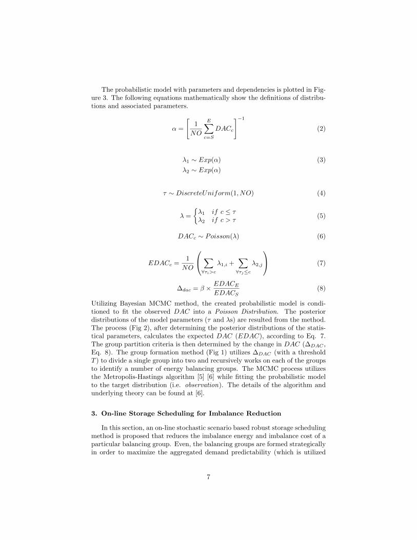
The probabilistic model with parameters and dependencies is plotted in Fig-ure 3. The following equations mathematically show the definitions of distribu-tions and associated parameters.

α =

[1

NO

E∑c=S

DACc

]−1(2)

λ1 ∼ Exp(α) (3)

λ2 ∼ Exp(α)

τ ∼ DiscreteUniform(1, NO) (4)

λ =

{λ1 if c ≤ τλ2 if c > τ

(5)

DACc ∼ Poisson(λ) (6)

EDACc =1

NO

∑∀τi>c

λ1,i +∑∀τj≤c

λ2,j

(7)

∆dac = β × EDACEEDACS

(8)

Utilizing Bayesian MCMC method, the created probabilistic model is condi-tioned to fit the observed DAC into a Poisson Distribution. The posteriordistributions of the model parameters (τ and λs) are resulted from the method.The process (Fig 2), after determining the posterior distributions of the statis-tical parameters, calculates the expected DAC (EDAC), according to Eq. 7.The group partition criteria is then determined by the change in DAC (∆DAC ,Eq. 8). The group formation method (Fig 1) utilizes ∆DAC (with a thresholdT ) to divide a single group into two and recursively works on each of the groupsto identify a number of energy balancing groups. The MCMC process utilizesthe Metropolis-Hastings algorithm [5] [6] while fitting the probabilistic modelto the target distribution (i.e. observation). The details of the algorithm andunderlying theory can be found at [6].

3. On-line Storage Scheduling for Imbalance Reduction

In this section, an on-line stochastic scenario based robust storage schedulingmethod is proposed that reduces the imbalance energy and imbalance cost of aparticular balancing group. Even, the balancing groups are formed strategicallyin order to maximize the aggregated demand predictability (which is utilized

7

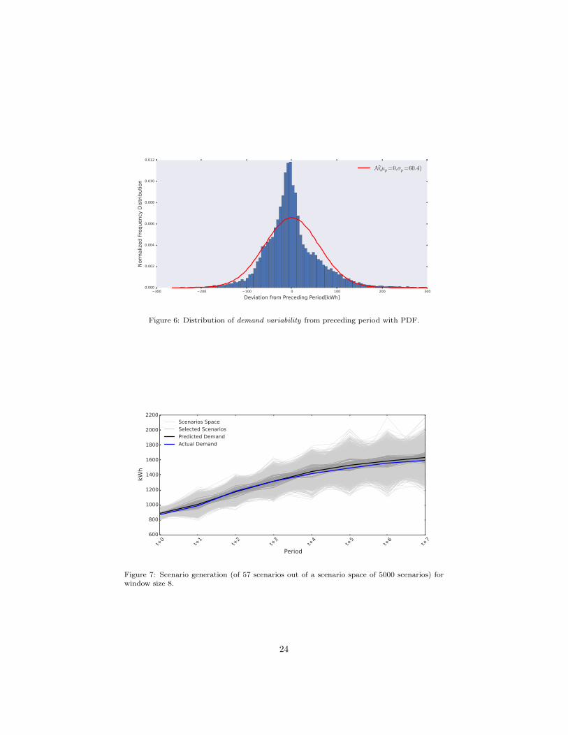
in the forward and day-ahead market to determine supply contract), in real-time, the imbalance of energy is still inevitable due to the prediction error. ThePPS, therefore, interacts with the Energy Imbalance Market (EIM) to nullifythe imbalance (by purchasing in case of demand is higher than the contractedsupply or by selling otherwise). The price setting of EIM is considerably highercompared with conventional energy tariff. Exemplary imbalance pricing schemeis shown in Figure 4 [3]. The pricing scheme follows a nonlinear curve where ahigher penalty has to be paid by PPS if the imbalance energy goes beyond athreshold (in Fig. 4 the threshold is set as 50kWh), in case of buying from EIM.On the other hand, PPS will receive no additional revenue if the energy to besold is higher than the threshold (-50kWh). The threshold is set as 3% of themonthly peak supply, according to [3].

Figure 4: Non-linear convex imbalance pricing scheme.Therefore, reducing imbalance energy and cost are narrowed down to op-

timizing the non-linear convex imbalance pricing curve by controlling storagecharge/discharge power. To this end, we propose a stochastic sliding windowbased charge/discharge (CD) algorithm (that is designed based on the con-cept of MPC), which will reduce the imbalance energy (with imbalance cost)by intelligently charging/discharging spatially distributed energy storages (e.g.battery). We refer the method as Stochastic Sliding Window based CD algo-rithm (S-SWCD). The system outline for S-SWCD is described in Figure 5. Thesystem receives (at a particular period t) contracted supply for a short window(let’s say for next w periods), aggregated demand of recent past, and currentmeasured status of the batteries (state-of-charge, SOC) and produces an opti-mal CD schedule for a number of batteries that eventually reduce the imbalanceenergy and imbalance cost and are robust against the demand uncertainty. TheOptimization Module consists of an MILP solver that is responsible for produc-ing robust CD scheduling after minimizing the expected imbalance energy andimbalance cost. Although, the module produces CD scheduling for the nextw periods, only the 1st CD schedule (which is for period t) is applied to thebattery system and the rest of the schedules are discarded. S-SWCD provides aclosed loop solution since a feedback policy is implemented to compensate thedemand variability and uncertainty. The subsequent sections will describe thecomponents of the system.

Figure 5: Outline of S-SWCD algorithm with components.

3.1. Short-term Demand Predictor

A Support Vector Machine (SVM) [21] based time series prediction method-ology is applied in order to predict the demand by utilizing the historic demandinformation. The demand signal is a time series, which follows a certain trendline (regulated by e.g. periods, weekdays, holidays, etc.). SVM finds optimalregression (Support Vector Regression, SVR) models while minimizing the train-ing error and model complexity. The developed SVR based demand predictionengine models the (recent) past demand patterns to predict demand for a shortwindow (for a window size of w, typically for next 4-hours). At a certain pe-

riod t, the predictor produces the estimated demand D̃mt to D̃mt+w−1 using

8

the historical demand till t − 1. This expression can be written as D̃mt+i|t−1,i = 0, ..., w − 1. The predictor creates w separate models for each of the laggedperiods. For example, while predicting demand D̃mt|t−1, SVR engine createsand trains the model (of lag 1) by fitting a particular demand Dmi with a non-linear mapping of its previous demands, starting from demand at t− 1 down todemand at a particular training horizon. Note that, the training data set onlyconsiders the recent demand set (instead of the whole data set) to avoid over-training the model by seasonally differed demand data. SVR tries to generatethe non-linear model as the following function f lmodel for lag l (l = 0, ..., w− 1),

f lmodel : [Dmi−l−1, Dmi−l−2, ..., Dmi−NP−1, Fi] 7→ Dmi (9)

where i = t− TH − 1, ..., t− 1, TH is the training horizon, NP is the numberof past periods, Fi is additional feature vector containing influential temporalinformation such as, holiday/weekend indicator, time of the day, and day ofthe week. The radial basis function is used as SVM kernel that transformsthe data into a higher dimensional space while performing the regression. Thehyper-parameters for creating the appropriate model are fixed by performingappropriate number of cross-validations within fractions of training data (so-called through grid-search).

However, the predicted demand for a particular period tends to change dueto uncertainty. For example, D̃mt+2|t is not necessarily similar to D̃mt+2|t+1.That is, the predicted demand at 12:00 when predicting at 11:00 is not necessar-ily same as when predicting at 11:30. Which is why, a deterministic objectivefunction is not capable of handling the uncertainty imposed by the demandpredictor. Therefore, a stochastic scenario based optimization approach is un-dertaken that minimizes the expected imbalance energy and imbalance cost.The next section focuses on the Scenario Generator.

3.2. Scenario Generator

A scenario, in this context, is actually a randomized snapshot of a predicteddemand signal. The scenario is generated by utilizing the demand predictionerror information coupled with the variability from the demand of preceding pe-riod. The system gradually learns the prediction errors (that are realized so far)for each of the lagged periods, l and determines the probability density function,PDF of the prediction error. The PDF of the prediction errors is a GaussianDistribution with almost zero mean and a specific standard deviation (let’s callit the error PDF ; N (µl, σl)). On the other hand, the PDF of the demand vari-ability from the preceding period follows the Gaussian Distribution as well, asshown in Figure 6 (let’s call it the variability PDF; N (µp, σp)). Therefore, thepredicted demand scenarios are generated by collecting samples in a BivariateGaussian Distribution of error PDF and variability PDF. There are severalways to generate statistical scenarios, such as utilizing nonlinear programmingfor multi-stage decision problem [22]). However, sophisticated method as asrequires higher computational power which goes against the speed requirementfor an on-line operation. Therefore, we adopted a simpler yet effective ways to

9

generate scenarios. Initially, a large scenario space is generated utilizing theaforementioned Bivariate Gaussian Distribution. The distribution is shown inthe following equation

dl(s ∈ S) ∼ N (µ,Σ) (10)

where µ contains the 2D-vector of means containing the µl and µp, and Σ is thecovariance matrix containing the variances, shown as

Σ =

[σ2l σ2

p

σ2p σ2

l

](11)

Therefore, the predicted demand for scenario s ∈ S is determined as following

D̃mt+l|t−1,s = D̃mt+l|t−1 + dl(s) (12)

Figure 6: Distribution of demand variability from preceding period withPDF.

where D̃mt+l|t−1,s is the predicted demand scenario for lag l and D̃mt+l|t−1is the predicted demand (from Demand Predictor module) at period t+ l, pre-dicted at period t − 1. However, the scenario space too large to be integratedinto the optimization. Therefore, the space must be reduced (the so-called sce-nario reduction). The reduction process is conducted by taking a subset of

the scenario space, S ⊂ S. The elements D̃mt+l|t−1,s for s ∈ S are chosenby considering the sum-of-squared distance from the baseline predicted demandsignals, D̃mt+l|t−1. Figure 7 shows a case of scenario generation for a particularpredicted demand signal (considering w = 8, number of scenarios = 57 and a30-minutes granularity) with associated scenario space.

Figure 7: Scenario generation (of 57 scenarios out of a scenario space of5000 scenarios) for window size 8.

3.3. Optimization Module

The optimization module reduces the imbalance energy and imbalance costfor a particular window (utilizing the predicted demand signals and scenarios)while deciding the storage charge/discharge schedule and associated power dis-patch. The module however, utilizes the decision regarding CD schedule anddispatch for the current period while discarding the rest. At the next cycle,the module slides the window one time step and repeats the process (so called,closed-loop system).

3.3.1. Objective Function with Constraints

The problem is a multi-objective (due to imbalance energy and imbalancecost minimization) and stochastic optimization problem. The imbalance energyand imbalance cost need to be optimized separately due to non-linearity in thecost function (Figure 4). The scalarized version of the stochastic optimizationproblem is described in Eq. 13. The 1st part of the objective function describesthe absolute reduction of imbalance energy (weighted by c0) while the 2nd partis about reduction of associated imbalance cost (weighted by c1). Utilizing only

10

imbalance cost as the objective will make the PPS intentionally increase theimbalance energy (by deliberately charging the battery up) so that it can sellthe energy in later time, thereby, staying at the left side of the imbalance pricingcurve. By incorporating the imbalance energy separately and performing themulti-objective optimization (with a small scaler weight given to the imbalanceenergy reduction), the system sustains a certain regulations on the energy andprice trade-off. However, the system can always perform a single objective (onlythe imbalance cost, for instance) if it is the expected behavior by setting thecorresponding weight as zero.

minimizeXi,b,Pi,b

E[FC(X,P )]

:=∑s∈S

Pr(s)×

c0 ×

t+w−1∑i=t

|Imi,s|+

c1 ×t+w−1∑i=t

IC(Imi,s)

(13)

where FC is the cost function comprising the weighted imbalance energy andcost, S is the predicted demand scenario set and Pr(s) is the probability assignedto scenario s (is set as 1/|S|). The imbalance energy for a scenario s ∈ S isformulated as (Eq. 14).

Imi,s = Spi − D̃mi,s −∑b∈B

Pi,b (14)

where Spi is the contracted supply at period i and D̃mi,s is the predicteddemand at period i for scenario s. The imbalance cost function, IC is a convexand non-linear function that can be presented by Figure 4. The IC containsboth cost part (when demand is higher than the supply) and revenue part (whensupply is higher than the demand). Pi,b is the power dispatch (+ve for charging,-ve for discharging) from/to a battery b over a set of batteries B. The storagedynamics are presented as the following constraint.

Xi,b = Xi−1,b + ηb × Pi,b (15)

Xb,min ≤ Xi,b ≤ Xb,max (16)

−pd,b ≤ Pi,b ≤ pc,b (17)

Eq. 13 is the discrete time energy status (state-of-charge, SOC) of b at period i(considering ∆t = 15), where the efficiency ηb is composed of charging efficiencyηcb and discharging efficiency ηdb (as shown in Eq. 18).

ηb =

{ηcb , if Pi,b ≥ 0

1/ηdb , otherwise(18)

5thereby making Pi,b as energy dispatch at period i (done for simplification)

11

Eq. 14 bounds the SOC within a particular limit while Eq. 15 shows the powercharging/discharging limit (pc,b and pd,b, respectively). Due to the non-linearityin objective function (Eq. 13) and constraints (e.g. conditional CD efficiencyat Eq. 18), the optimization problem needs to be (equivalently) transformedinto an MILP problem. The section to come describes the equivalent MILPformation of the above optimization problem.

3.3.2. MILP Transformation

In this section, the transformation of objective function (Eq. 13) and con-straints to facilitate MILP formulations are presented. The storage dynamicsappeared in Eq. (13-15) can be effectively transformed into a linear formulationby introducing the following additional variables

Si,b =

{1 if Pi,b ≥ 00 otherwise

(19)

Axi,b = Si,b × Pi,b (20)

Therefore, utilizing MLD system formulation of converting logical dynamics toMILP [8], the storage SOC dynamics can be transformed to

Xi,b = Xi−1,b + (ηcb − 1/ηdb )×Axi,b − 1/ηdb × Pbi,b (21)

The non-linear logical constraints in Eq. (17-18) are equivalently casted to linearconstraints [7] and handled together with charging/discharging power limit ofstorage (Eq. 15). The followings shows the casted linear equations.

pd,b × Si,b − Pi,b − pd,b ≤ 0 (22)

−pd,b × Si,b + Pi,b ≤ 0 (23)

pd,b × Si,b +Axi,b − Pi,b − pd,b ≤ 0 (24)

pd,b × Si,b −Axi,b + Pi,b − pd,b ≤ 0 (25)

−pc,b × Si,b +Axi,b ≤ 0 (26)

−pc,b × Si,b −Axi,b ≤ 0 (27)

The non-linear and convex cost function requires to be linearized to be fittedinto the MILP formulation. The transformation is conducted by introducingadditional mixed-integer variables. For the sake of simplicity, we remove thescenario s notation of original equations. The imbalance cost is equivalentlytransformed into a segmented combination of sub-costs (for a particular periodi, as shown in below)

ICi = IC(Imib) =

NPS∑k=1

PSk × Zi,k (28)

where PSk, k = 1, ..., NPS is the k-th imbalance unit price and NPS is thenumber of price segments6. The imbalance energy is constrained to be the sum

6As of Figure 4, the pricing scheme has 4 unit price segments activated by an energythreshold (i.e. ±50 kWh). There, PS1 = 45.7, PS2 = 15.0, PS3 = 10.48, and PS4 = 0

12

of segmented energies, i.e.

Imi =

NPS∑k=1

Zi,k (29)

The activation of Zi,k is controlled by binary variables Y . Considering Th(as imbalance energy threshold, e.g. 50 kWh as of Figure 4), a big numberM = 1e+7 and NPS = 4; the following constraints are added to the formulationas a measure of activating appropriate Zi,k (avoiding the subscript i)

(Th−M)× Y1 ≤ Z1 ≤ (Th−M)× Y0−Th ≤ Z2

Th× Y3 ≤ Z3 ≤ Th× Y20 ≤ Z4 ≤M × Y3

Note that, the above equations can be generalized to work with any value ofNPS. Some additional constraints are required to limit the activation in one ofthe halves of the pricing curve. The absolute value in the imbalance energy inEq. 13 is transformed into an equivalent function by introducing the lower- andupper-bound variables (since absolute value imposes non-linearity and cannotbe readily solvable by MILP).

4. Numerical Simulations and Discussions

This section presents the numerical simulations, analysis, results and discus-sions associated with formation of balancing groups and robust CD scheduling.A total of 103 apartments building in Tokyo are taken as customers and theirdemand data are utilized for the analysis. More particularly, the demand dataof January and February, 2013 are taken and broken down to two phases

1. Analysis and training phase: Data from January 1st to January 20th areutilized to perform the balancing group formation and train the initialprediction (SVR) model.

2. Optimization and simulation phase: Data from January 21st to February28th are utilized to perform simulation regarding robust and on-line CDscheduling. Note that, although the initial SVR model is trained utilizingdemand data from Jan. 1st to Jan. 20th (i.e. 20 days), the SVR modelis kept updated using the immediate past 20-days demand data (from thesimulation day). For example, while performing simulation for Jan. 25th,the demand data from Jan. 5th to Jan. 24th are utilized.

The algorithms are implemented in Python programming language. TheBayesian MCMC based group formation algorithm is implemented in conjunc-tion with PyMC package [23], an open-source Python package to perform Bayesian

(JPY/kWh)[3].

13

analysis. The open-source solver [9] is used to solve the MILP in robust CDscheduling.

4.1. Formation of Balancing Groups

The 1st part of this section describes the analysis and results regarding en-ergy balancing group formation. The demand data has a 30-minutes granularity.The MDSD (i.e. DAC) of each customer are determined according to Eq. 1considering demands from January 1st, 2013 to January 20th, 2013.

Figure 8: Divide-and-conquer process of group formation: Status of dacVec-tor.

The divide-and-conquer process of group formation with associated dacV ector(Figure 1) range is shown in Figure 8. The corresponding articulated customersat each stage of division are also pointed out in the figure. For example, initiallythe dacV ector contains customers from 1 to 103, [1, 103]. After performing theBayesian MCMC sampling method on dacV ector, customer 84 is selected asarticulated customer (AC) and hence serves as the dividing point (1st Phase).The posterior distributions of the model parameters τ and λs at 1st Phase areplotted in Figure 9. The distributions of τ identifies customer 84 as AC since itis highly likely to be one. Note that, the prior of τ was a uniform distribution,which is changed after performing the Bayesian MCMC sampling process andprovides a posterior that correctly maps to the target true distribution (i.e. ob-servation). The distributions of DACs (i.e. λs, before and after τ , respectively)are shown in the figure as well. Although, the λs were set as Exponential Dis-tributions as priors, the posteriors come out as Normal Distributions throughthe Bayesian inference. In the process of MCMC, a total number of 80,000 ran-dom samples are generated utilizing the prior distributions of model parameters.Among them 25% of the samples are discarded (so called burn-in [5] of samplessince the convergence of the Markov Chain is not fully known) while tracing theposterior samples. Referring back to Figure 8, at the next phase, the dacV ectoris divided into two child vectors of [1, 84] and [85, 103], each of which will gothrough the Bayesian MCMC process.The process is repeated until the vectoris not further divisible (i.e. ∆dac is below a point, T ), and thereby formingbalancing groups. Finally, the process settles down forming 4 balancing groups.

Figure 10 shows the result of Bayesian MCMC based demand aggregationand resultant balancing groups (the customers are already ordered accordingto their DSD). At the same time, the figure points out the expected DSDper customer in a group. For example, Group 1 (G1), that contains 57 cus-tomers, has an expected DSD of 7.83kWh per customer. As a by-product ofBayesian MCMC method, the posterior distribution of DSD over the customersin G1 is evaluated, which is also printed in Figure 10 as a Normal Distribution.The periodical (half-hourly) aggregated DSD for each group is shown in Fig-ure 11. Evidently, the Bayesian MCMC based demand aggregation strategyforms groups whose DSDs are close to each other even when the group sizesare different. That establishes the proposed demand aggregation strategy is aneffective clustering strategy of relatively heterogeneous demand signals.

14

Figure 9: The posterior distributions of τ and λs after performing BayesianMCMC at 1st Phase .

Figure 10: Group formation using Bayesian MCMC based aggregation strat-egy.

Figure 11: Resultant (periodical) demand standard deviation for each group.

4.2. Robust CD Scheduling of Energy Storage

At the 2nd part, we will investigate the on-line robust energy storage schedul-ing (S-SWCD) to reduce imbalance energy and cost for Group 1 (G1). The G1contains 57 customers. The first 20 days’ (January 1 to 20) demand data isutilized to train the initial demand predictor model, which gives us 38 days(approximately) to perform the on-line CD scheduling algorithm and evaluatethe performance. The peak demand (kWh/30-minutes) for the first 20-days isrecorded as 2,500kWh/30-minutes.

In order to perform the short-term demand prediction, prediction windowsize, w is set as 8. The initial scenario space, S contains 5000 scenarios. Finally,the number of scenarios in the reduced scenario set, S is set as 57. The values ofw and |S| are settled to 8 and 57, respectively based on the sensitivity analysisof these parameters on the imbalance cost reduction while keeping the batterycapacity fixed. As an energy storage, Lithium-ion Battery is utilized. The size ofthe battery (power rating and consequently energy capacity) are determined byanalyzing the DAC distribution (e.g. as in Figure 10), since DAC is essentiallyMDSD which in turn represents the peak potential deviation that requires tobe minimized by battery. The expected DAC for G1, 7.83kWh/customer, canbe utilized as battery size (that makes an approximated 445kWh of aggregatedbattery capacity for G1). However, due to higher accuracy in day-ahead pre-diction, the aggregated DAC (i.e. potential battery capacity) of 445kWh canbe treated as an upper-bound. In the experiment, we present the results con-sidering aggregated battery capacity of 320kWh. At the same time, the powerrating of the aggregated batteries is considered as 640 kW (i.e. the batteries areof 2E ratings). A total of 50 batteries (of rating 6.4kWh/12.8kW, SOC limit of1% to 96% and C/D round-trip efficiency of 95%) are assumed to be installedat G1. These batteries are operated and controlled (via PPS’s SCADA system)synchronously. Therefore, the simulations are performed considering aggregatedbattery capacity and aggregated SOC. We assume a day-ahead prediction error(i.e. the basic imbalance due to deviation between contracted supply and actualdemand) Normally Distributed around 0 mean and having 10% (of demand) as astandard deviation. The imbalance energy threshold beyond which the penaltytariff is applied is set as 93kWh (3% of the maximum contracted supply)[3].

The performance of SVR based short-term demand predictor is describedin Figure 12. The lag-wise error distributions (standard deviations) follow apattern where the errors are relatively lower in smaller lags. The accumulatederror distribution over all lags are depicted in the lower right corner of the fig-ure. The errors are normally distributed (N (−0.59, 125.25kWh)) with a MeanAbsolute Percent Error (MAPE) of 6.27%. The prediction accuracy is thereforegood enough to be utilized at the on-line optimization. In order to generate

15

scenarios, the lag-based error statistics (mean and standard deviation, as of Eq.12) is utilized. The generated scenarios are referred back to Figure 7.

Figure 12: Prediction error statistics (lag-based) with combined error distri-bution.

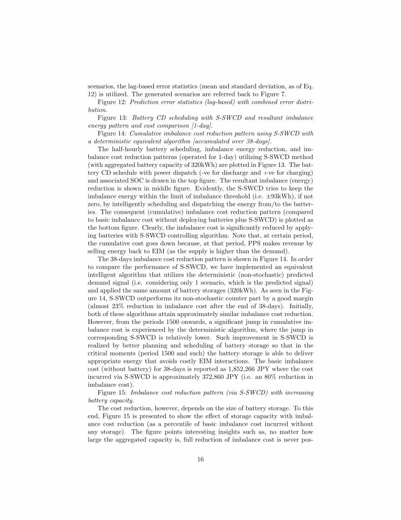
Figure 13: Battery CD scheduling with S-SWCD and resultant imbalanceenergy pattern and cost comparison [1-day].

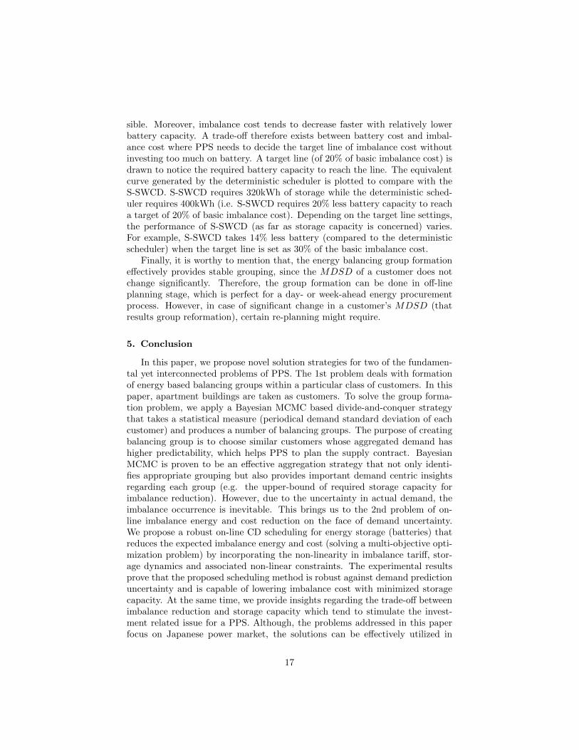
Figure 14: Cumulative imbalance cost reduction pattern using S-SWCD witha deterministic equivalent algorithm [accumulated over 38-days].

The half-hourly battery scheduling, imbalance energy reduction, and im-balance cost reduction patterns (operated for 1-day) utilizing S-SWCD method(with aggregated battery capacity of 320kWh) are plotted in Figure 13. The bat-tery CD schedule with power dispatch (-ve for discharge and +ve for charging)and associated SOC is drawn in the top figure. The resultant imbalance (energy)reduction is shown in middle figure. Evidently, the S-SWCD tries to keep theimbalance energy within the limit of imbalance threshold (i.e. ±93kWh), if notzero, by intelligently scheduling and dispatching the energy from/to the batter-ies. The consequent (cumulative) imbalance cost reduction pattern (comparedto basic imbalance cost without deploying batteries plus S-SWCD) is plotted asthe bottom figure. Clearly, the imbalance cost is significantly reduced by apply-ing batteries with S-SWCD controlling algorithm. Note that, at certain period,the cumulative cost goes down because, at that period, PPS makes revenue byselling energy back to EIM (as the supply is higher than the demand).

The 38-days imbalance cost reduction pattern is shown in Figure 14. In orderto compare the performance of S-SWCD, we have implemented an equivalentintelligent algorithm that utilizes the deterministic (non-stochastic) predicteddemand signal (i.e. considering only 1 scenario, which is the predicted signal)and applied the same amount of battery storages (320kWh). As seen in the Fig-ure 14, S-SWCD outperforms its non-stochastic counter part by a good margin(almost 23% reduction in imbalance cost after the end of 38-days). Initially,both of these algorithms attain approximately similar imbalance cost reduction.However, from the periods 1500 onwards, a significant jump in cumulative im-balance cost is experienced by the deterministic algorithm, where the jump incorresponding S-SWCD is relatively lower. Such improvement in S-SWCD isrealized by better planning and scheduling of battery storage so that in thecritical moments (period 1500 and such) the battery storage is able to deliverappropriate energy that avoids costly EIM interactions. The basic imbalancecost (without battery) for 38-days is reported as 1,852,266 JPY where the costincurred via S-SWCD is approximately 372,860 JPY (i.e. an 80% reduction inimbalance cost).

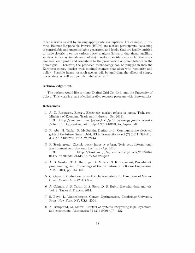
Figure 15: Imbalance cost reduction pattern (via S-SWCD) with increasingbattery capacity.

The cost reduction, however, depends on the size of battery storage. To thisend, Figure 15 is presented to show the effect of storage capacity with imbal-ance cost reduction (as a percentile of basic imbalance cost incurred withoutany storage). The figure points interesting insights such as, no matter howlarge the aggregated capacity is, full reduction of imbalance cost is never pos-

16

sible. Moreover, imbalance cost tends to decrease faster with relatively lowerbattery capacity. A trade-off therefore exists between battery cost and imbal-ance cost where PPS needs to decide the target line of imbalance cost withoutinvesting too much on battery. A target line (of 20% of basic imbalance cost) isdrawn to notice the required battery capacity to reach the line. The equivalentcurve generated by the deterministic scheduler is plotted to compare with theS-SWCD. S-SWCD requires 320kWh of storage while the deterministic sched-uler requires 400kWh (i.e. S-SWCD requires 20% less battery capacity to reacha target of 20% of basic imbalance cost). Depending on the target line settings,the performance of S-SWCD (as far as storage capacity is concerned) varies.For example, S-SWCD takes 14% less battery (compared to the deterministicscheduler) when the target line is set as 30% of the basic imbalance cost.

Finally, it is worthy to mention that, the energy balancing group formationeffectively provides stable grouping, since the MDSD of a customer does notchange significantly. Therefore, the group formation can be done in off-lineplanning stage, which is perfect for a day- or week-ahead energy procurementprocess. However, in case of significant change in a customer’s MDSD (thatresults group reformation), certain re-planning might require.

5. Conclusion

In this paper, we propose novel solution strategies for two of the fundamen-tal yet interconnected problems of PPS. The 1st problem deals with formationof energy based balancing groups within a particular class of customers. In thispaper, apartment buildings are taken as customers. To solve the group forma-tion problem, we apply a Bayesian MCMC based divide-and-conquer strategythat takes a statistical measure (periodical demand standard deviation of eachcustomer) and produces a number of balancing groups. The purpose of creatingbalancing group is to choose similar customers whose aggregated demand hashigher predictability, which helps PPS to plan the supply contract. BayesianMCMC is proven to be an effective aggregation strategy that not only identi-fies appropriate grouping but also provides important demand centric insightsregarding each group (e.g. the upper-bound of required storage capacity forimbalance reduction). However, due to the uncertainty in actual demand, theimbalance occurrence is inevitable. This brings us to the 2nd problem of on-line imbalance energy and cost reduction on the face of demand uncertainty.We propose a robust on-line CD scheduling for energy storage (batteries) thatreduces the expected imbalance energy and cost (solving a multi-objective opti-mization problem) by incorporating the non-linearity in imbalance tariff, stor-age dynamics and associated non-linear constraints. The experimental resultsprove that the proposed scheduling method is robust against demand predictionuncertainty and is capable of lowering imbalance cost with minimized storagecapacity. At the same time, we provide insights regarding the trade-off betweenimbalance reduction and storage capacity which tend to stimulate the invest-ment related issue for a PPS. Although, the problems addressed in this paperfocus on Japanese power market, the solutions can be effectively utilized in

17

other markets as well by making appropriate assumptions. For example, in Eu-rope, Balance Responsible Parties (BRPs) are market participants, consistingof controllable and uncontrollable generators and loads, that are legally entitledto trade electricity on the various power markets (forward, day-ahead, ancillaryservices, intra-day, imbalance markets) in order to satisfy loads within their con-trol area, earn profit and contribute to the preservation of power balance in thepower grid. Therefore, the proposed methodology can be plugged-in into theEuropean energy market with minimal changes that align with regularity andpolicy. Possible future research avenue will be analyzing the effects of supplyuncertainty as well as dynamic imbalance tariff.

Acknowledgement

The authors would like to thank Digital Grid Co., Ltd. and the University ofTokyo. This work is a part of collaborative research program with these entities.

References

[1] A. N. Resources, Energy, Electricity market reform in japan, Tech. rep.,Ministry of Economy, Trade and Industry (Oct 2014).URL http://www.meti.go.jp/english/policy/energy_environment\

/electricity_system_reform/pdf/201410EMR_in_Japan.pdf

[2] R. Abe, H. Taoka, D. McQuilkin, Digital grid: Communicative electricalgrids of the future, Smart Grid, IEEE Transactions on 2 (2) (2011) 399–410.doi:10.1109/TSG.2011.2132744.

[3] P. Study-group, Electric power industry reform, Tech. rep., InternationalEnvironment and Economy Institute (Apr 2013).URL http://ieei.or.jp/wp-content/uploads/2013/04/

8e4776f6f89c3d5cb1d531d3f7fe6e23.pdf

[4] A. D. Gordon, T. A. Henzinger, A. V. Nori, S. K. Rajamani, Probabilisticprogramming, in: Proceedings of the on Future of Software Engineering,ACM, 2014, pp. 167–181.

[5] C. Geyer, Introduction to markov chain monte carlo, Handbook of MarkovChain Monte Carlo (2011) 3–48.

[6] A. Gelman, J. B. Carlin, H. S. Stern, D. B. Rubin, Bayesian data analysis,Vol. 2, Taylor & Francis, 2014.

[7] S. Boyd, L. Vandenberghe, Convex Optimization, Cambridge UniversityPress, New York, NY, USA, 2004.

[8] A. Bemporad, M. Morari, Control of systems integrating logic, dynamics,and constraints, Automatica 35 (3) (1999) 407 – 427.

18

[9] P. Coin-OR, Cbc, coin-or branch and cut (2010).URL http://projects.coin-or.org/Cbc

[10] J. G. Dias, S. B. Ramos, Dynamic clustering of energy markets: An ex-tended hidden markov approach, Expert Systems with Applications 41 (17)(2014) 7722 – 7729.

[11] G. Chicco, Overview and performance assessment of the clustering methodsfor electrical load pattern grouping, Energy 42 (1) (2012) 68 – 80.

[12] G. Chicco, R. Napoli, F. Piglione, Comparisons among clustering tech-niques for electricity customer classification, IEEE Transactions on PowerSystems 21 (2) (2006) 933–940.

[13] S. Haben, C. Singleton, P. Grindrod, Analysis and clustering of residentialcustomers energy behavioral demand using smart meter data, Smart Grid,IEEE Transactions on 7 (1) (2016) 136–144.

[14] R. Firestone, C. Marnay, Energy manager design for microgrids, LawrenceBerkeley National Laboratory.

[15] R. Palma-Behnke, C. Benavides, F. Lanas, B. Severino, L. Reyes, J. Llanos,D. Saez, A microgrid energy management system based on the rolling hori-zon strategy, Smart Grid, IEEE Transactions on 4 (2) (2013) 996–1006.

[16] P. Meibom, R. Barth, B. Hasche, H. Brand, C. Weber, M. O’Malley,Stochastic optimization model to study the operational impacts of highwind penetrations in ireland, Power Systems, IEEE Transactions on 26 (3)(2011) 1367–1379.

[17] R. Wang, P. Wang, G. Xiao, A robust optimization approach for energygeneration scheduling in microgrids, Energy Conversion and Management106 (2015) 597 – 607.

[18] Y. Ma, J. Matuko, F. Borrelli, Stochastic model predictive control for build-ing hvac systems: Complexity and conservatism, IEEE Transactions onControl Systems Technology 23 (1) (2015) 101–116.

[19] A. Viana, J. P. Pedroso, A new milp-based approach for unit commitmentin power production planning, International Journal of Electrical Power &Energy Systems 44 (1) (2013) 997–1005.

[20] M. Carrion, J. M. Arroyo, A computationally efficient mixed-integer linearformulation for the thermal unit commitment problem, IEEE Transactionson Power Systems 21 (3) (2006) 1371–1378.

[21] C. J. Burges, A tutorial on support vector machines for pattern recognition,Data mining and knowledge discovery 2 (2) (1998) 121–167.

[22] K. Høyland, S. W. Wallace, Generating scenario trees for multistage deci-sion problems, Management Science 47 (2) (2001) 295–307.

19

[23] A. Patil, D. Huard, C. J. Fonnesbeck, Pymc: Bayesian stochastic modellingin python, Journal of statistical software 35 (4) (2010) 1.

20

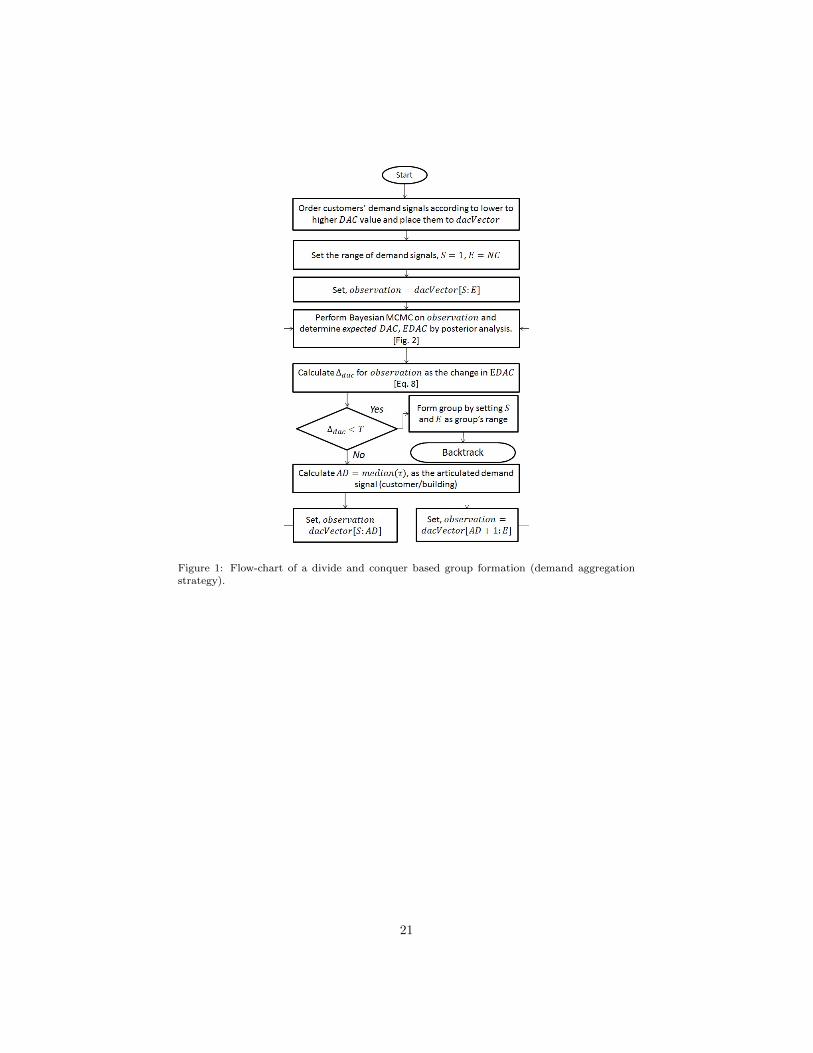
Figure 1: Flow-chart of a divide and conquer based group formation (demand aggregationstrategy).

21

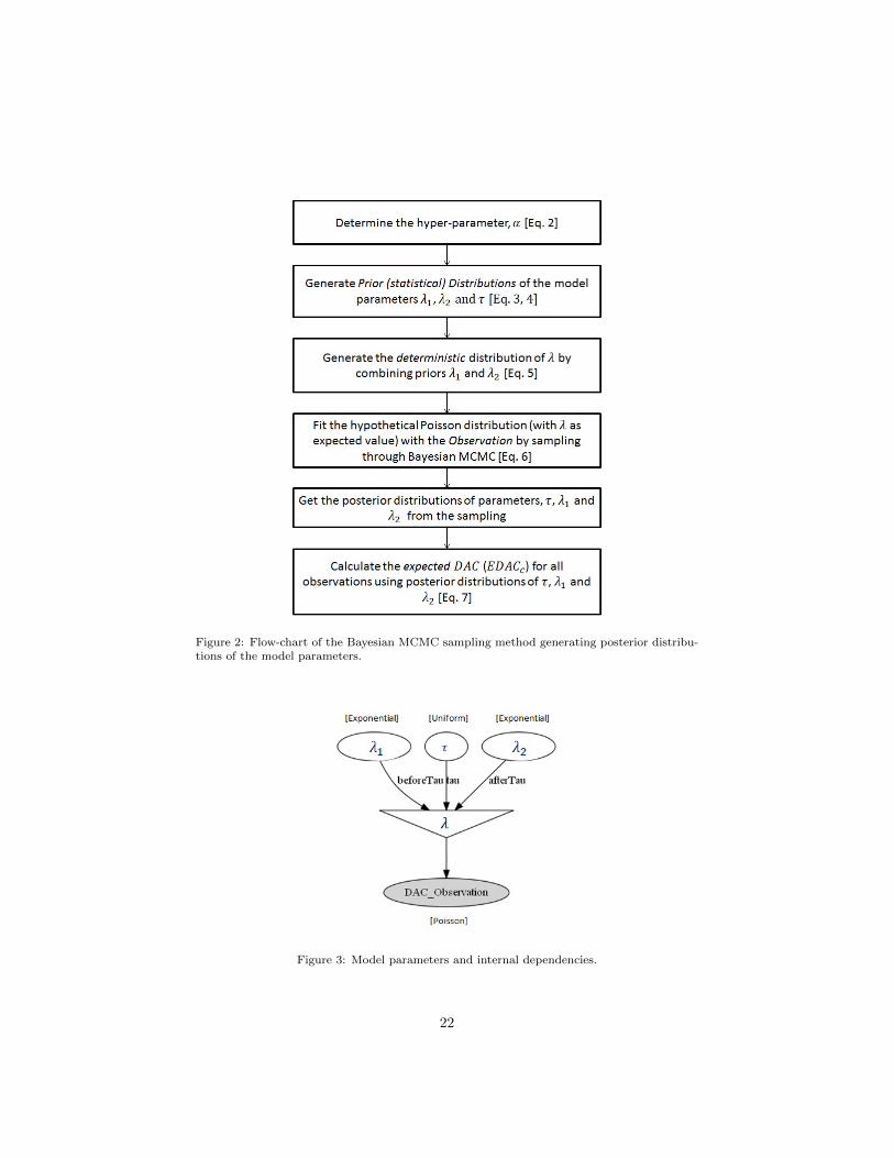
Figure 2: Flow-chart of the Bayesian MCMC sampling method generating posterior distribu-tions of the model parameters.

Figure 3: Model parameters and internal dependencies.

22

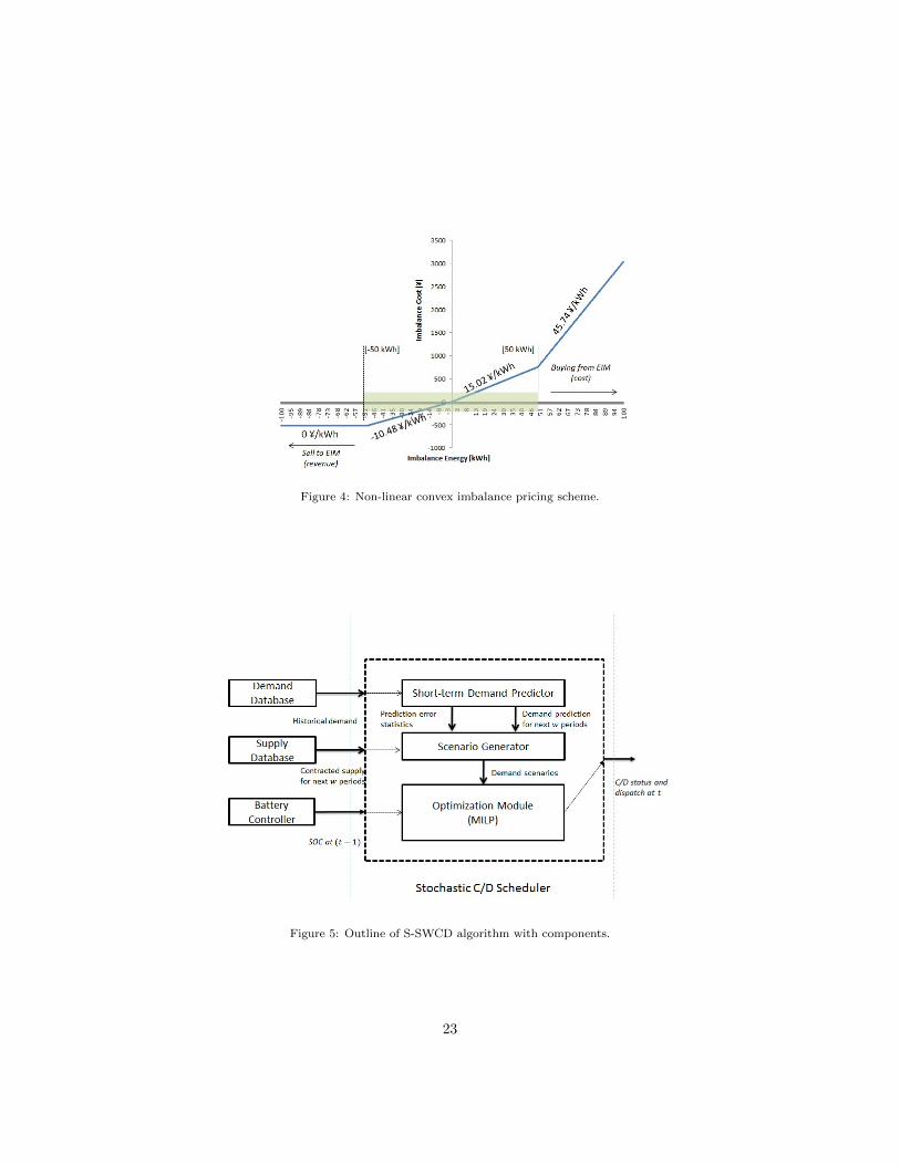
Figure 4: Non-linear convex imbalance pricing scheme.

Figure 5: Outline of S-SWCD algorithm with components.

23

−300 −200 −100 0 100 200 300

Deviation from Preceding Period[kWh]

0.000

0.002

0.004

0.006

0.008

0.010

0.012

Norm

alized F

requency D

istr

ibuti

on

N(µp=0,σ

p=60.4)

Figure 6: Distribution of demand variability from preceding period with PDF.

t+0

t+1

t+2

t+3

t+4

t+5

t+6

t+7

Period

600

800

1000

1200

1400

1600

1800

2000

2200

kW

h

Scenarios Space

Selected Scenarios

Predicted Demand

Actual Demand

Figure 7: Scenario generation (of 57 scenarios out of a scenario space of 5000 scenarios) forwindow size 8.

24

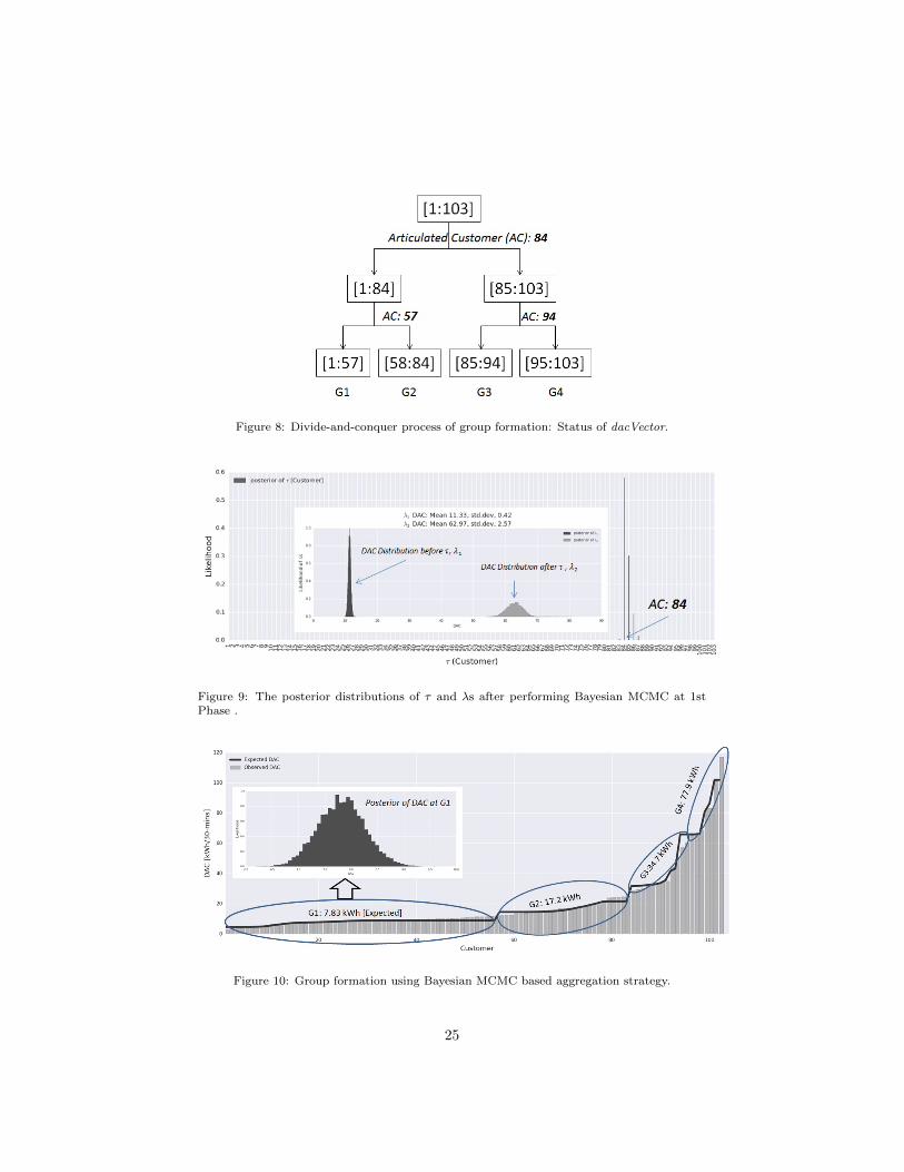
Figure 8: Divide-and-conquer process of group formation: Status of dacVector.

Figure 9: The posterior distributions of τ and λs after performing Bayesian MCMC at 1stPhase .

Figure 10: Group formation using Bayesian MCMC based aggregation strategy.

25

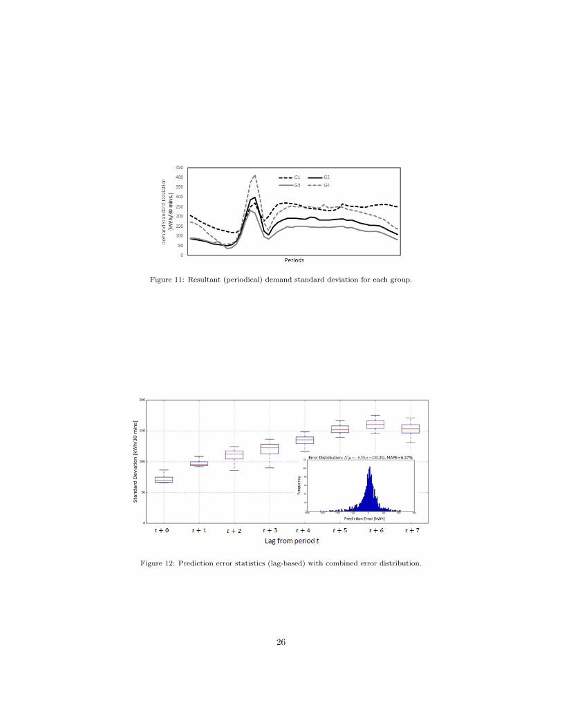
Figure 11: Resultant (periodical) demand standard deviation for each group.

Figure 12: Prediction error statistics (lag-based) with combined error distribution.

26

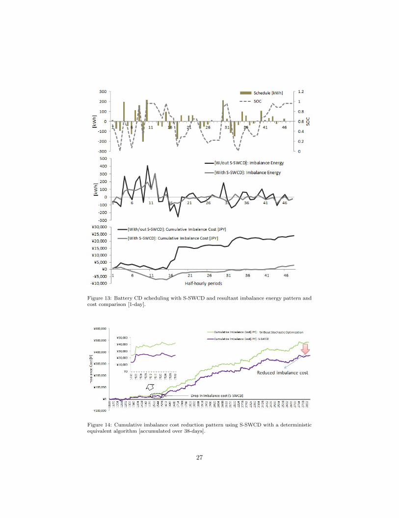
Figure 13: Battery CD scheduling with S-SWCD and resultant imbalance energy pattern andcost comparison [1-day].

Figure 14: Cumulative imbalance cost reduction pattern using S-SWCD with a deterministicequivalent algorithm [accumulated over 38-days].

27

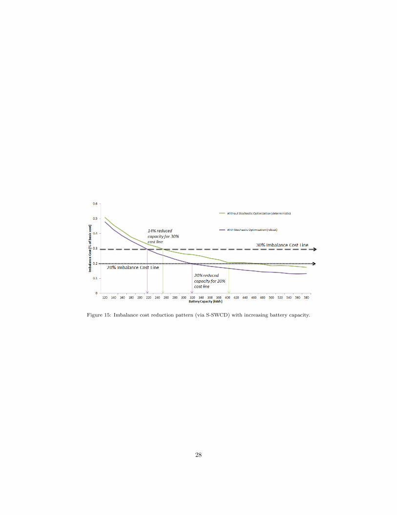
Figure 15: Imbalance cost reduction pattern (via S-SWCD) with increasing battery capacity.

28