Robust Controller Design and PID Tuning for

Multivariable Processes

Wen Tan

Department of AutomationNorth China Electric Power University

Zhuxinzhuang, DewaiBeijing, 102206

P. R. ChinaE-mail: wtan@ieee.org

Tongwen Chen1 and Horacio J. Marquez

Department of Electrical & Computer EngineeringUniversity of Alberta

Edmonton, AB T6G 2V4Canada

E-mail: {tchen,marquez}@ee.ualberta.ca

Abstract

In this paper, a robust controller design method is first formulated to deal with both

performance and robust stability specifications for multivariable processes. The optimum

problem is then dealt with using a loop-shaping H∞ approach, which gives a sub-optimal

solution. Then a PID approximation method is proposed to reduce a high-order controller.

The whole procedure involves selecting several parameters and the computation is simple,

so it serves as a PID tuning method for multivariable processes. Examples show that the

method is easy to use and the resulting PID settings have good time-domain performance

and robustness.

Keywords: PID Tuning; Robust Control; Loop-shaping H∞ Control; Multivariable Pro-

cesses; Structured Singular Value.

1To whom all correspondence should be addressed. Phone: (780) 492-3334. Fax: (780) 492-1811

1 Introduction

Despite the enormous interest that modern control techniques have sparked among academics

during the last three or four decades, PID controllers are still preferred in industrial process

control. The reason is that controllers designed with the aid of modern control techniques are

usually of high order, difficult to implement, and virtually impossible to re-tune on line. PID

controllers, on the other hand, are simple, easy to implement, and comparatively easy to re-tune

on line.

Roughly speaking, there are three different approaches to obtain PID controller parameters:

1. Tune the parameters of the PID structure following one of several available tuning tech-

niques. Examples of these techniques include:

• SISO processes: Ziegler-Nichols (Z-N) method [1], internal-model-control (IMC)

based method [2], optimization method [3], and gain-phase margin method [4].

• MIMO processes: See references [5]-[9].

Even though PID controllers are relatively easy to tune for single loop processes, the

underlying theory for multiloop processes is still immature. For example, the gain-phase

margin criterion or optimization criterion is not well suited for multivariable processes.

2. Assume that the controller has a PID structure, and find the PID parameters using some

well-known optimization methods, e.g., H∞ [10], mixed H2�H∞ [11] and semidefinite

programming approaches [12]. These methods can be used to obtain the PID controller

parameters such that the controllers have good time-domain performance and frequency-

domain robustness. The main problem with this approach is that the fixed-structured

controller design is not convex in the controller parameter space. As a consequence it is

not easy to find a globally optimal set of parameters. Even when a solution can be found,

it is usually at the expense of time-consuming computations. For example, for a 2� 2

process with decentralized PID controller in [12], it took 2 hours to find the 6 parameters

on a Pentium II 333MHz computer.

3. Design a controller of an arbitrary structure using any advanced technique, and then re-

duce it or approximate it to one with a PID structure. Reference [13] is an example for

1

this method: First an IMC controller is designed, then it is reduced to one with a PID

form. The same idea is adopted in [14] for single-loop systems, where a loop-shaping H∞

technique is used. The problem with this method is that although the performance of the

closed-loop system might be guaranteed for the full-order controller, it is not so for the

reduced-order controller. Caution must be taken when reducing a full-order controller to

a PID one.

The first approach is what we called ‘controller tuning’, while the second is ‘controller design’.

The difference between ‘design’ and ‘tuning’ is roughly as follows:

• For controller design we usually need a somewhat detailed model and a detailed specifi-

cation of the control objectives; while for controller tuning a rough model is enough. It

can be done even without a model.

• For controller tuning, there are several parameters which reflect the control objectives,

and the controller parameters vary according to the chosen parameters and should be

obtained with little effort.

If a design method does not require a detailed process model, the control objectives can be

related to several easily understood parameters, and little effort is needed to compute the con-

troller, then it can serve as a tuning method. The third category above is just such methods. It

combines the advantages of the first two categories.

In this paper we will first propose a robust controller design method that is suitable for

tuning purposes, and relate it to loop-shaping H∞ design [15]. Then we propose a method to

approximate a high-order state-space controller with a PID one. Combining the two procedures,

we obtain a PID tuning method for multivariable processes. Examples show that this method is

simple to use and it can find well-tuned PID parameters for a variety of multivariable processes.

2 Robust Controller Design

It is well-known that a well-designed control system should meet the following requirements

besides the nominal stability:

• Disturbance attenuation

2

• Setpoint tracking

• Robust stability and/or robust performance

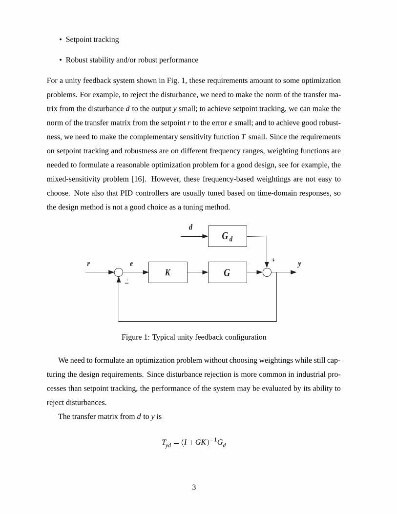
For a unity feedback system shown in Fig. 1, these requirements amount to some optimization

problems. For example, to reject the disturbance, we need to make the norm of the transfer ma-

trix from the disturbance d to the output y small; to achieve setpoint tracking, we can make the

norm of the transfer matrix from the setpoint r to the error e small; and to achieve good robust-

ness, we need to make the complementary sensitivity function T small. Since the requirements

on setpoint tracking and robustness are on different frequency ranges, weighting functions are

needed to formulate a reasonable optimization problem for a good design, see for example, the

mixed-sensitivity problem [16]. However, these frequency-based weightings are not easy to

choose. Note also that PID controllers are usually tuned based on time-domain responses, so

the design method is not a good choice as a tuning method.

K Gr y

_

G d

e

d

+

Figure 1: Typical unity feedback configuration

We need to formulate an optimization problem without choosing weightings while still cap-

turing the design requirements. Since disturbance rejection is more common in industrial pro-

cesses than setpoint tracking, the performance of the system may be evaluated by its ability to

reject disturbances.

The transfer matrix from d to y is

Tyd � �I �GK��1Gd

3

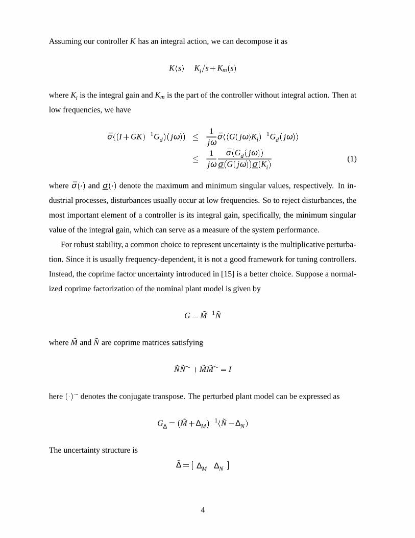
Assuming our controller K has an integral action, we can decompose it as

K�s� � Ki�s�Km�s�

where Ki is the integral gain and Km is the part of the controller without integral action. Then at

low frequencies, we have

σ��I�GK��1Gd�� jω�� �1jω

σ��G� jω�Ki��1Gd� jω��

�1jω

σ�Gd� jω��

σ�G� jω��σ�Ki�(1)

where � and � denote the maximum and minimum singular values, respectively. In in-

dustrial processes, disturbances usually occur at low frequencies. So to reject disturbances, the

most important element of a controller is its integral gain, specifically, the minimum singular

value of the integral gain, which can serve as a measure of the system performance.

For robust stability, a common choice to represent uncertainty is the multiplicative perturba-

tion. Since it is usually frequency-dependent, it is not a good framework for tuning controllers.

Instead, the coprime factor uncertainty introduced in [15] is a better choice. Suppose a normal-

ized coprime factorization of the nominal plant model is given by

G � M�1N

where M and N are coprime matrices satisfying

NN�� MM� � I

here ���� denotes the conjugate transpose. The perturbed plant model can be expressed as

G∆ � �M�∆M��1�N �∆N�

The uncertainty structure is

∆ � � ∆M ∆N �

4

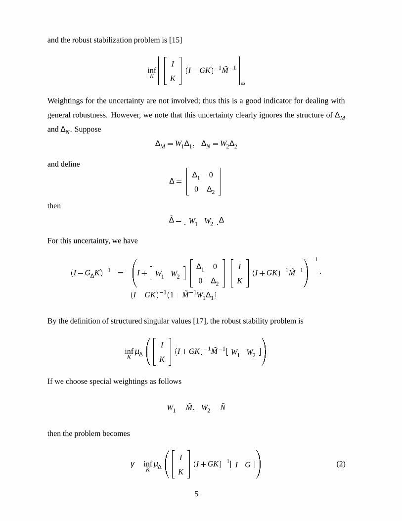
and the robust stabilization problem is [15]

infK

�������� I

K

���I �GK��1M�1

������∞

Weightings for the uncertainty are not involved; thus this is a good indicator for dealing with

general robustness. However, we note that this uncertainty clearly ignores the structure of ∆M

and ∆N . Suppose

∆M �W1∆1� ∆N �W2∆2

and define

∆ �

�� ∆1 0

0 ∆2

��

then

∆ � � W1 W2�∆

For this uncertainty, we have

�I�G∆K��1 �

��I �

�W1 W2

�� ∆1 0

0 ∆2

���� I

K

���I �GK��1M�1

��1

�

�I �GK��1�1� M�1W1∆1�

By the definition of structured singular values [17], the robust stability problem is

infK

µ∆

���� I

K

���I �GK��1M�1� W1 W2

�

�

If we choose special weightings as follows

W1 � M� W2 � N

then the problem becomes

γ � infK

µ∆

���� I

K

���I �GK��1� I G �

� (2)

5

We note that now the class of perturbed plant is

G∆ � �M� M∆1��1�N � N∆2� � �I�∆1�

�1G�I �∆2�

so it can represent simultaneous input multiplicative and inverse output multiplicative uncertain-

ties. If we treat a disturbance as a model uncertainty, then this perturbation model can represent

simultaneous input and output disturbances. To summarize, this is a better robustness indicator

for tuning, and there is no need to choose weightings.

For a single-loop system, it is not difficult to show that

γ � maxω

��S� jω��� �T � jω���

The value approximates 1 at low and high frequencies and the maximum normally occurs at the

mid-range frequency. Compared with the usual tuning indicators such as Ms, the peak of the

sensitivity function, and Mp, the peak of the complementary sensitivity function, the indicator

is more appropriate since it bounds both Ms and Mp simultaneously.

From the discussion above, we would like to make the integral gain as large as possible

and make the robust stability indicator as large as possible. Unfortunately, large integral action

will violate the robust stability requirement. So trade-off is needed for a reasonable controller

design. In summary, we need to design a controller such that

maxσ�Ki�

under the constraint

γ � µ∆

���� I

K

�� �I �GK��1� I G �

�� γm

where γm is a given robust stability requirement. The problem is to maximize the integral action

under the constraint of a certain degree of robust stability, a generalization of the idea used in

[18, 19] for single-loop processes.

6

3 Loop shaping H∞ approach

The problem proposed in the previous section is a nonconvex optimization problem and is hard

to solve directly. However, the loop-shaping H∞ approach provides a solution to a sub-optimal

problem. To show that, we first review the loop-shaping H∞ approach. Details can be found in

[15].

Given a plant G, the loop-shaping H∞ design proceeds as follows:

• Loop Shaping: A pre-compensator W1 and/or post-compensator W2 are used to shape the

singular values of G so that the shaped plant G �W2GW1 has a desired open-loop shape

(Roughly speaking, the desired open-loop shapes should have large magnitudes at the low

frequencies and small at high frequencies, while the roll-off rates should not be too large

at the mid-range frequencies.)

• Robust Stabilization: For the shaped plant G, solve the robust stabilization problem:

ε�1max � inf

K

�������� I

K

���I � GK��1M�1

������∞

(3)

where M�1N is a normalized left coprime factorization of the shaped plant G.

• The final feedback controller is constructed as K �W1KW2

It is interesting to note that the problem in (3) is a sub-optimal one to that in (2) [20]. Since

� M N � is a unit, then

�������� I

K

���I � GK��1M�1

������∞

�

�������� I

K

��M�1� M N �

������∞

�

�������� I

K

�� �I� GK��1� I G �

������∞

�

�������� W2 0

0 W�11

���� I

K

�� �I�GK��1� I G �

�� W�1

2 0

0 W1

��������

∞

(4)

So if W2 and W1 commute with uncertainty ∆1 and ∆2, respectively, then it is an upper bound

7

for the structured singular value, thus

µ∆

���� I

K

�� �I�GK��1� I G �

��

�������� W2 0

0 W�11

���� I

K

���I �GK��1� I G �

�� W�1

2 0

0 W1

��������

∞

Since ∆1 and ∆2 are assumed to be full block, if we choose the compensators as diagonal, then

they commute with the uncertainty, and we can have a suboptimal solution.

The performance on Ki can be also reflected in the compensator choice. Since the integral

action is usually imposed on the pre-compensator W1 and the H∞ controller computed from (3)

does not contain any integrator, thus the integral action of the final controller is affected by the

integral action of W1. So instead of directly solving the problem in (2), we can solve by first

specifying the integral action of W1, then find controller to satisfy the robustness requirement.

We should point out that the H∞-optimization problem in (3) can be solved explicitly without

iteration, and the H∞ problem is always regular and only requires the solution of two Riccati

equations. So the effort to compute the controller is little once the compensators are chosen.

For controller tuning purpose, we can simplify the compensator choice by setting the post-

compensator W2 as an identity matrix and the pre-compensator W1 as a diagonal PI one. The

reasons for just using a PI instead of a more sophisticated high-order pre-compensator are as

follows:

1. Our final controller will be approximated by a PID one. Comparing with a simple PI

pre-compensator, a high-order pre-compensator might result in a better H∞ controller but

not a better PID controller due to the approximation. It may not be worth to find more

sophisticated open-loop shapes.

2. The time-domain performance of the closed-loop system is affected by the PI parameters

just as in a single-loop process, which makes it possible to tune the final PID controller

by tuning the diagonal PI pre-compensator.

3. As pointed out in [21] for single-loop processes, a PI pre-compensator is the ‘best’ for

input disturbance rejection.

We note that in the usual loop-shaping design procedure [15] for multivariable processes,

the pre-compensator has two parts

W1 �WaWi

8

where Wa is usually chosen as a static decoupler and Wi is diagonal. Usually Wa is not diagonal,

thus W1 does not commute with ∆2. So the uncertainty which the problem in (3) tries to stabilize

is only for the shaped plant, not the actual plant, which is the main source of criticism for the

method. We note that the closed-loop system will show good disturbance rejection as long as the

integral action is reasonable; the coupling of the process will only affect the setpoint tracking.

So in loop-shaping design we can first ignore the coupling effect of a multivariable process, and

after the design we can choose a setpoint filter to modify the setpoint tracking properties. For

example, in a 2�2 system, the final setpoint filter has the following form:

F �

�� 1 � f1

� f2 1

��

To completely decouple the setpoint responses, f1 and f2 should be chosen as

f1 � T�111 T12� f2 � T�1

22 T21

where T is the complementary sensitivity matrix and the subscripts refer to its denoted elements.

To realize, a first-order approximation can be used. Note that T12 and T21 have derivative action;

so the filter will have the form of asbs�1 . In general, we can choose the setpoint filter as

F�s� �

�� 1

λ11s�1 �λ12s

λ12s�1

�λ21s

λ21s�11

λ22s�1

��

where the parameters are tuned to reduce the overshoots and the coupling in the setpoint re-

sponses.

4 PID Approximation

It is known that the H∞ controllers designed using two Riccati equations are of the same order

as that of the generalized plant; so the order of the final controller may be high. We need to

adopt some controller reduction method to get a PID controller. It is unrealistic to require a

PID controller to be as robust as a high-order controller and at the same time to have the same

performance. Two approximations are possible:

9

• Retain the performance with a sacrifice on robustness.

• Retain the robustness with a sacrifice on performance.

Since the model uncertainty we use is not fully structured, the robust stability condition is suf-

ficient but not necessary; so we choose to sacrifice robustness instead of performance. Further-

more, this approximation is simpler to obtain than the one retaining robustness, since it might

be impossible for a PID controller to have the same robustness as a high-order controller.

Reference [13] proposed to use a (truncated) Maclaurin series as an approximation to IMC

controllers in order to find the PID parameters. It was shown that this technique works well

for many processes. Here we adopt the same technique to find PID approximation to H∞ con-

trollers: Unlike the IMC method which is usually done in the frequency domain, we propose

the following procedure to find PID parameters directly in the state-space domain.

Consider now a controller K�s�, given by a state-space realization of the form

� � x � Akx�Bky� Ak � ℜ n�n� Bk � ℜ n�p�

u �Ckx�Dky� Ck � ℜ q�n� Bk � ℜ q�q�

Let the rank of the matrix Ak be r. Note that r � n since by incorporating W1 into the controller,

Ak always has at least one eigenvalue at the origin. The multiplicity of the zero eigenvalue of

Ak is n� r. We assume that there exist n� r linearly independent eigenvectors for this zero

eigenvalue. Then we find a similarity transformation T such that

TAkT�1 �

�� 0 0

0 A2

�� �

where A2 � ℜ r�r is nonsingular. This transformation can be computed using the eigenvalue

decomposition of Ak. With this T , the new state-space realization is given by

� �

˙x � Akx� Bky�

u � Ckx� Dky�

10

with Ak � TAkT�1, Dk � Dk, and

Ck �CkT�1 ��

C1 C2

� Bk � T Bk �

�� B1

B2

�� �

A PID approximation of the form

KPID�s� � Kp �Ki�s�Kds

can now be obtained by truncating the Maclaurin expansion of the controller with respect to the

variable s:

K�s� ��

C1 C2

�� sI 0

0 sI�A2

���1�� B1

B2

���Dk

�C1B1

s��Dk�C2A�1

2 B2��C2A�22 B2s� � � � �

Here we assume s� σ�A2� since we are most interested in the low frequency band. So we have

Kp � Dk�C2A�12 B2� Ki �C1B1� Kd ��C2A�2

2 B2� (5)

It is then clear that based on this reduction procedure, the resulting PID controller achieves

good approximation of the controller K at low frequencies, especially the integral action, so we

can expect that the resulting PID controller will retain the disturbance rejection performance

of the high-order controller. The following steps need to be considered after the reduction

procedure:

1. Due to the minimum-phase requirement of a PID controller, the signs of the proportional

gain, the integral gain and the differentiator should be the same. So if the corresponding

elements of Kp, Ki and Kd in (5) do not have the same sign, then we need to discard the

term that has the opposite sign with the element in Ki, which is the most important term.

2. The derivative action should be taken with care. We find that a PID approximation with

ideal differentiator s sometimes destabilizes a process even though the original high-order

controller works well. This seldom happens for single-loop processes, but it is quite

11

common for multivariable processes. We believe the reason is that the phase information

of the original controller is lost when using an ideal differentiator. Thus, a filter of the

form 1α s�1 should be used for the differentiator.

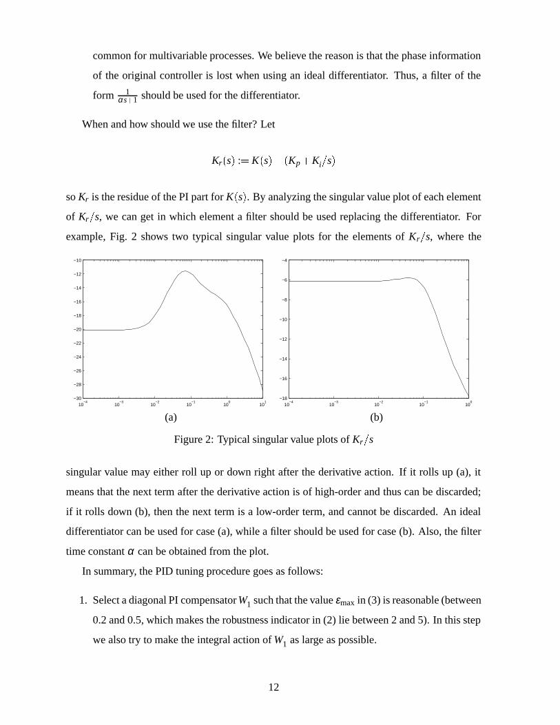
When and how should we use the filter? Let

Kr�s� :� K�s�� �Kp�Ki�s�

so Kr is the residue of the PI part for K�s�. By analyzing the singular value plot of each element

of Kr�s, we can get in which element a filter should be used replacing the differentiator. For

example, Fig. 2 shows two typical singular value plots for the elements of Kr�s, where the

10−4

10−3

10−2

10−1

100

101

−30

−28

−26

−24

−22

−20

−18

−16

−14

−12

−10

10−4

10−3

10−2

10−1

100

−18

−16

−14

−12

−10

−8

−6

−4

(a) (b)

Figure 2: Typical singular value plots of Kr�s

singular value may either roll up or down right after the derivative action. If it rolls up (a), it

means that the next term after the derivative action is of high-order and thus can be discarded;

if it rolls down (b), then the next term is a low-order term, and cannot be discarded. An ideal

differentiator can be used for case (a), while a filter should be used for case (b). Also, the filter

time constant α can be obtained from the plot.

In summary, the PID tuning procedure goes as follows:

1. Select a diagonal PI compensator W1 such that the value εmax in (3) is reasonable (between

0.2 and 0.5, which makes the robustness indicator in (2) lie between 2 and 5). In this step

we also try to make the integral action of W1 as large as possible.

12

2. Approximate the resulting H∞ controller with a PID one using the procedure described in

this section.

3. If necessary, tune a setpoint filter to decouple the setpoint responses.

4. If the time-domain performance is unsatisfactory, follow the idea of tuning single-loop PI

controllers to find another pre-compensator, and repeat the above steps.

Finally, we remark that the PID approximation might fail if the high-order parts of the

original controllers are quite critical for the system stability and robustness.

5 Simulation Study

Two examples are used to illustrate the tuning procedure proposed.

Example 1: Consider the pilot scale distillation column model reported by Wood and Berry [22]:

G�s� �

�� 12�8e�s

16�7s�1�18�9e�3s

21s�1

6�6e�7s

10�9s�1�19�4e�3s

14�4s�1

��

The process is highly coupled and attracts much attention in the literature. For the proposed

method, we tune the pre-compensator as:

W1 �

�� 0�06�1�8s��s 0

0 0�04�1�8s��s

��

For this pre-compensator, εmax � 0�392.

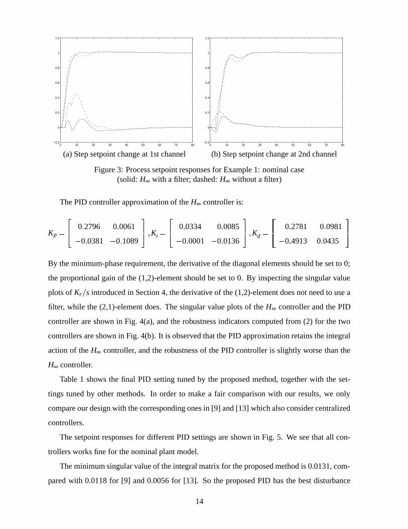
The setpoint responses of the H∞ controller are shown as the dashed lines in Fig. 3. The

responses are not decoupled, so a filter is tuned to decouple the setpoint tracking:

F �

�� 1 0

� 4s4s�1 1

��

The final responses with the filter is also shown as the solid lines in Fig. 3, where the coupling

effect is clearly reduced.

13

0 10 20 30 40 50 60 70 80−0.2

0

0.2

0.4

0.6

0.8

1

1.2

0 10 20 30 40 50 60 70 80−0.2

0

0.2

0.4

0.6

0.8

1

1.2

(a) Step setpoint change at 1st channel (b) Step setpoint change at 2nd channel

Figure 3: Process setpoint responses for Example 1: nominal case(solid: H∞ with a filter; dashed: H∞ without a filter)

The PID controller approximation of the H∞ controller is:

Kp �

�� 0�2796 0�0061

�0�0381 �0�1089

�� �Ki �

�� 0�0334 �0�0085

�0�0001 �0�0136

�� �Kd �

�� �0�2781 �0�0981

�0�4913 0�0435

��

By the minimum-phase requirement, the derivative of the diagonal elements should be set to 0;

the proportional gain of the (1,2)-element should be set to 0. By inspecting the singular value

plots of Kr�s introduced in Section 4, the derivative of the (1,2)-element does not need to use a

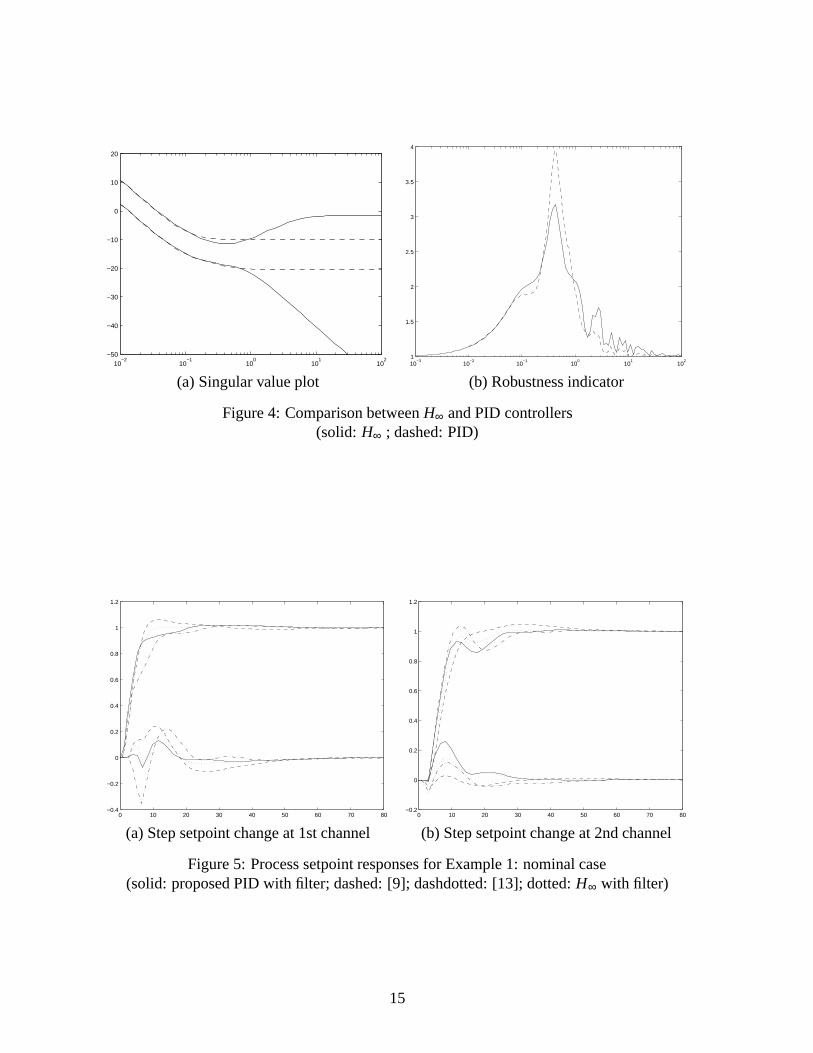
filter, while the (2,1)-element does. The singular value plots of the H∞ controller and the PID

controller are shown in Fig. 4(a), and the robustness indicators computed from (2) for the two

controllers are shown in Fig. 4(b). It is observed that the PID approximation retains the integral

action of the H∞ controller, and the robustness of the PID controller is slightly worse than the

H∞ controller.

Table 1 shows the final PID setting tuned by the proposed method, together with the set-

tings tuned by other methods. In order to make a fair comparison with our results, we only

compare our design with the corresponding ones in [9] and [13] which also consider centralized

controllers.

The setpoint responses for different PID settings are shown in Fig. 5. We see that all con-

trollers works fine for the nominal plant model.

The minimum singular value of the integral matrix for the proposed method is 0.0131, com-

pared with 0.0118 for [9] and 0.0056 for [13]. So the proposed PID has the best disturbance

14

10−2

10−1

100

101

102

−50

−40

−30

−20

−10

0

10

20

10−3

10−2

10−1

100

101

102

1

1.5

2

2.5

3

3.5

4

(a) Singular value plot (b) Robustness indicator

Figure 4: Comparison between H∞ and PID controllers(solid: H∞ ; dashed: PID)

0 10 20 30 40 50 60 70 80−0.4

−0.2

0

0.2

0.4

0.6

0.8

1

1.2

0 10 20 30 40 50 60 70 80−0.2

0

0.2

0.4

0.6

0.8

1

1.2

(a) Step setpoint change at 1st channel (b) Step setpoint change at 2nd channel

Figure 5: Process setpoint responses for Example 1: nominal case(solid: proposed PID with filter; dashed: [9]; dashdotted: [13]; dotted: H∞ with filter)

15

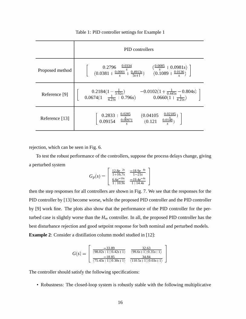
Table 1: PID controller settings for Example 1

PID controllers

Proposed method

�0�2796� 0�0334

s ��0�0085s �0�0981s�

��0�0381� 0�0001s � 0�4913s

5s�1 � ��0�1089� 0�0136s �

�

Reference [9]

�0�2184�1� 1

3�92s� �0�0102�1� 10�445s �0�804s�

�0�0674�1� 14�23s �0�796s� �0�0660�1� 1

4�25s�

�

Reference [13]

�0�2833� 0�0285

s ��0�04105� 0�02185s �

0�09154� 0�00971s ��0�121� 0�0148

s �

�

rejection, which can be seen in Fig. 6.

To test the robust performance of the controllers, suppose the process delays change, giving

a perturbed system

Gp�s� �

�� 12�8e�2s

1�16�7s�18�9e�4s

1�21s

6�6e�10s

1�10�9s�19�4e�4s

1�14�4s

��

then the step responses for all controllers are shown in Fig. 7. We see that the responses for the

PID controller by [13] become worse, while the proposed PID controller and the PID controller

by [9] work fine. The plots also show that the performance of the PID controller for the per-

turbed case is slightly worse than the H∞ controller. In all, the proposed PID controller has the

best disturbance rejection and good setpoint response for both nominal and perturbed models.

Example 2: Consider a distillation column model studied in [12]:

G�s� �

�� �33�89

�98�02s�1��0�42s�1�32�63

�99�6s�1��0�35s�1�

�18�85�75�43s�1��0�30s�1�

34�84�110�5s�1��0�03s�1�

��

The controller should satisfy the following specifications:

• Robustness: The closed-loop system is robustly stable with the following multiplicative

16

0 10 20 30 40 50 60 70 80−1

−0.5

0

0.5

1

1.5

2

2.5

3

3.5

0 10 20 30 40 50 60 70 80−7

−6

−5

−4

−3

−2

−1

0

1

(a) Input disturbance at 1st channel (b) Input disturbance at 2nd channel

Figure 6: Process disturbance responses for Example 1: nominal case(solid: proposed PID with filter; dashed: [9]; dashdotted: [13]; dotted: H∞ with filter)

0 10 20 30 40 50 60 70 80−0.6

−0.4

−0.2

0

0.2

0.4

0.6

0.8

1

1.2

1.4

0 10 20 30 40 50 60 70 80−0.2

0

0.2

0.4

0.6

0.8

1

1.2

1.4

(a) Step setpoint change at 1st channel (b) Step setpoint change at 2nd channel

Figure 7: Process setpoint responses for Example 1: perturbed case(solid: proposed PID with filter; dashed: [9]; dashdotted: [13]; dotted: H∞ with filter)

17

uncertainty ∆:

σ �∆� jω���

����100 jω�1jω�1000

����• Performance: The steady-state tracking error is less than 1/1000 for a step change in the

command signal. The settling time is expected to be within 5 minutes, i.e.,

���� s�10001000s�1

S�s�

����∞� 1

We tune the pre-compensator as

W1 �

�� 10�1�3s��s 0

0 10�1�3s��s

��

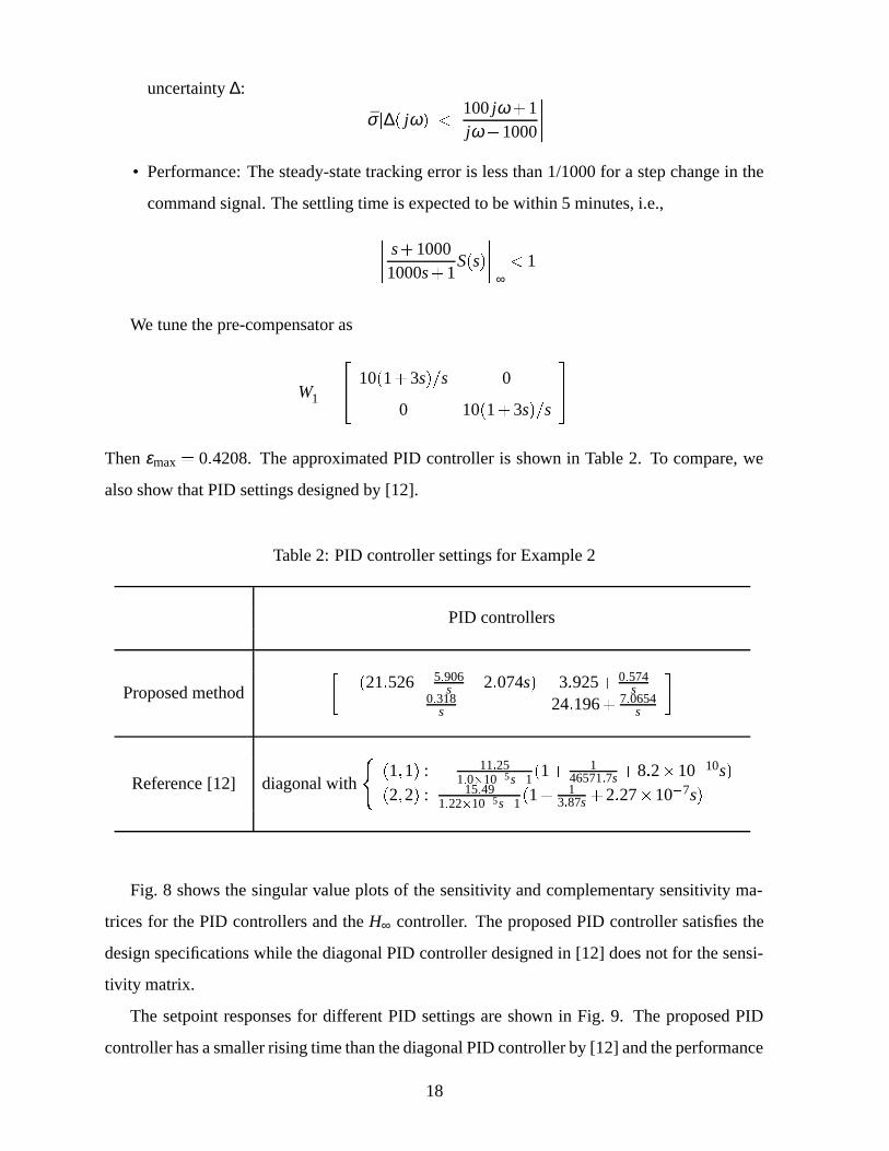
Then εmax � 0�4208. The approximated PID controller is shown in Table 2. To compare, we

also show that PID settings designed by [12].

Table 2: PID controller settings for Example 2

PID controllers

Proposed method

���21�526� 5�906

s �2�074s� 3�925� 0�574s

0�318s 24�196� 7�0654

s

�

Reference [12] diagonal with

��1�1� : � 11�25

1�0�10�5s�1�1� 1

46571�7s �8�2�10�10s�

�2�2� : 15�491�22�10�5s�1

�1� 13�87s �2�27�10�7s�

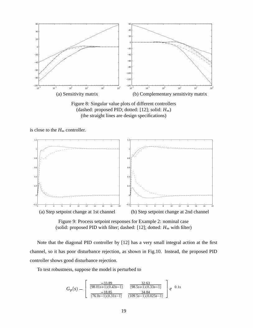
Fig. 8 shows the singular value plots of the sensitivity and complementary sensitivity ma-

trices for the PID controllers and the H∞ controller. The proposed PID controller satisfies the

design specifications while the diagonal PID controller designed in [12] does not for the sensi-

tivity matrix.

The setpoint responses for different PID settings are shown in Fig. 9. The proposed PID

controller has a smaller rising time than the diagonal PID controller by [12] and the performance

18

10−2

10−1

100

101

102

103

−100

−80

−60

−40

−20

0

20

40

60

10−2

10−1

100

101

102

103

−140

−120

−100

−80

−60

−40

−20

0

20

40

60

(a) Sensitivity matrix (b) Complementary sensitivity matrix

Figure 8: Singular value plots of different controllers(dashed: proposed PID; dotted: [12]; solid: H∞)

(the straight lines are design specifications)

is close to the H∞ controller.

0 2 4 6 8 10 12 14 16 18 20−0.2

0

0.2

0.4

0.6

0.8

1

1.2

0 2 4 6 8 10 12 14 16 18 20−0.2

0

0.2

0.4

0.6

0.8

1

1.2

(a) Step setpoint change at 1st channel (b) Step setpoint change at 2nd channel

Figure 9: Process setpoint responses for Example 2: nominal case(solid: proposed PID with filter; dashed: [12]; dotted: H∞ with filter)

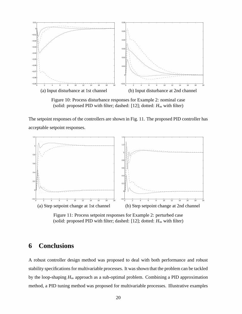
Note that the diagonal PID controller by [12] has a very small integral action at the first

channel, so it has poor disturbance rejection, as shown in Fig.10. Instead, the proposed PID

controller shows good disturbance rejection.

To test robustness, suppose the model is perturbed to

Gp�s� �

�� �33�89

�98�01s�1��0�43s�1�32�63

�98�5s�1��0�33s�1�

�18�85�76�0s�1��0�31s�1�

34�84�109�5s�1��0�025s�1�

��e�0�1s

19

0 2 4 6 8 10 12 14 16 18 20−0.09

−0.08

−0.07

−0.06

−0.05

−0.04

−0.03

−0.02

−0.01

0

0.01

0 2 4 6 8 10 12 14 16 18 20−0.01

0

0.01

0.02

0.03

0.04

0.05

0.06

(a) Input disturbance at 1st channel (b) Input disturbance at 2nd channel

Figure 10: Process disturbance responses for Example 2: nominal case(solid: proposed PID with filter; dashed: [12]; dotted: H∞ with filter)

The setpoint responses of the controllers are shown in Fig. 11. The proposed PID controller has

acceptable setpoint responses.

0 2 4 6 8 10 12 14 16 18 20−0.2

0

0.2

0.4

0.6

0.8

1

1.2

0 2 4 6 8 10 12 14 16 18 20−0.2

0

0.2

0.4

0.6

0.8

1

1.2

1.4

(a) Step setpoint change at 1st channel (b) Step setpoint change at 2nd channel

Figure 11: Process setpoint responses for Example 2: perturbed case(solid: proposed PID with filter; dashed: [12]; dotted: H∞ with filter)

6 Conclusions

A robust controller design method was proposed to deal with both performance and robust

stability specifications for multivariable processes. It was shown that the problem can be tackled

by the loop-shaping H∞ approach as a sub-optimal problem. Combining a PID approximation

method, a PID tuning method was proposed for multivariable processes. Illustrative examples

20

show that the method is easy to use and can find PID settings that have good time-domain

performance and robustness.

References

[1] J. G. Ziegler and N. B. Nichols, “Optimum settings for automatic controllers,” Trans.

ASME, vol. 62, pp. 759–768 (1942).

[2] M. Morari and E. Zafiriou, Robust Process Control. Englewood Cliffs NJ.: Prentice-Hall,

1989.

[3] M. Zhuang and D. P. Atherton, “Automatic tuning of optimum PID controllers,” IEE Proc.

on Control and Applications, vol. 140, pp. 216–224 (1993).

[4] W. K. Ho, C. C. Hang, and L. S. Cao, “Tuning of PID controllers based on gain and phase

margin specifications,” Automatica, vol. 31, no. 3, pp. 497–502 (1995).

[5] M. Zhuang and D. P. Atherton, “PID controller design for a TITO system,” IEE Proc. on

Control and Applications, vol. 141, pp. 111–120 (1994).

[6] A. P. Loh, C. C. Hang, G. K. Quek, and V. U. Vasnani, “Autotuning of multiloop

proportional-integral controller using relay feedback,” Ind. Eng. Chem. Res., vol. 32,

pp. 1102–1107 (1993).

[7] S. J. Shiu and S. H. Huang, “Sequential design method for multivariable decoupling and

multiloop PID controllers,” Ind. Eng. Chem. Res., vol. 37, pp. 107–119 (1998).

[8] A. Desbians, A. Pamerleau, and D. Hodouin, “Frequency based tuning of SISO controllers

for two-by-two processes,” IEE Proc. on Control and Applications, vol. 143, pp. 49–56

(1996).

[9] Q. G. Wang, Q. Zou, T. H. Lee, and Q. Bi, “Autotuning of multivariable PID controllers

from decentralized relay feedback,” Automatica, vol. 33, pp. 319–330 (1997).

[10] M. J. Grimble, “H∞ controllers with a PID structure,” Trans. ASME J. Dynam. Syst. Meas.

Control, vol. 112, pp. 325–330 (1990).

21

[11] B. S. Chen, Y. M. Chiang, and C. H. Lee, “A genetic approach to mixed H2/H∞ optimal

PID control,” IEEE Control System Magazine, vol. 15, pp. 51–56 (1995).

[12] J. Bao, J. F. Forbes, and P. J. McLellan, “Robust multiloop PID controller design: a succes-

sive semidefinite programming approach,” Ind. Eng. Chem. Res., vol. 38, pp. 3407–3413

(1999).

[13] J. W. Dong and G. B. Brosilow, “Design of robust multivariable PID controllers via IMC,”

Proc. American Control Conference, (Albuquerque, New Mexico), pp. 3380–3384 (1997).

[14] W. Tan, J. Z. Liu, and P. K. S. Tam, “PID tuning based on loop-shaping H∞ control,” IEE

Proc. on Control and Applications, vol. 145, pp. 485–490 (1998).

[15] D. C. McFarlane and K. Glover, Robust Controller Design Using Normalized Coprime

Factorization Description. Springer-Verlag, 1990.

[16] H. Kwakernaak, “Minimax frequency domain performance and robustness optimization

of linear feedback systems,” IEEE Trans. Automat. Contr., pp. 994–1004 (1985).

[17] J. C. Doyle, “Analysis of feedback systems with structured uncertainties,” IEE Proc. on

Control and Applications, vol. 129, pp. 242–250 (1982).

[18] K. J. Astrom, H. Panagopoulos, and T. Hagglund, “Design of PI controllers based on

non-convex optimization,” Automatica, vol. 34, no. 5, pp. 585–601 (1998).

[19] H. Panagopoulos and K. J. Astrom, “PID control design and H∞ loop shaping,” Proc. IEEE

Conf. on Control Applications, Hawaii, USA, pp. 103–108 (1999).

[20] E. J. M. Geddes and I. Postlethwaite, “An H∞ based loop shaping method and µ-synthesis,”

Proc. IEEE Conf. on Decision and Control, Brighton, England, pp. 533–538 (1991).

[21] S. Skogestad and I. Postlethwaite, Multivariable Feedback Control: Analysis and Design.

Wiley, 1996.

[22] R. K. Wood and M. W. Berry, “Terminal composition control of a binary distillation col-

umn,” Chem. Eng. Sci., vol. 28, pp. 1707–1712 (1973).

22