ROBUST CONTROL OF INTERVAL PLANTS: - …ymzhang/Papers/Interval Control Paper.doc · Web viewinterval model, predictive control, welding. 1. INTRODUCTION Interval models are useful

Zhang YM, Kovacevic R: Robust control of interval plants: A time domain method. IEE P-CONTR THEOR AP 144 (4): 347-353 JUL 1997

ROBUST CONTROL OF INTERVAL PLANTS: A TIME-DOMAIN METHOD

Y. M. Zhang and R. Kovacevic

ABSTRACT

A time-domain algorithm is proposed to control interval plants described by impulse response

functions. The closed-loop control actions are determined based on the interval ranges of the

model parameters. Robust steady-state performance in tracking a given set-point can be

guaranteed if the sign of the static gain is certain despite possible open-loop overshooting, delay,

and nonminimum phase of the interval plants. Simulation examples are given to illustrate the

performance. An application example in welding process control is also included.

Key words: interval model, predictive control, welding.

1. INTRODUCTION

Interval models are useful descriptions for many uncertain dynamic processes. Much of the

present success in interval plant control is restricted to analysis issues [1-9]. However, limited

progress has been made in achieving an effective systematic design method for the interval plant

control [4]. Preliminary results on the regularity of the robust design problem with respect to the

controller coefficients were obtained by Vicino and Tesi [10]. Recently, Abdallah et al. [11],

and Olbrot & Nikodem [12] addressed a class of interval plants with one interval parameter.

However, due to the complexity of the polynomial based analysis, the issue of controller

synthesis for uncertain systems with more independent interval parameters has not been solved.

It still “remains to a large extent an open and difficult problem” [4].

__________________________________________________________________________

The authors are with the Center for Robotics and Manufacturing Systems, University of Kentucky, Lexington, Kentucky 40506, USA.

1


In this work, a prediction based algorithm is proposed to control interval plants. Robust

steady-state performance in tracking a given set-point is guaranteed if the sign of the static gain

of the interval plant remains fixed when the parameters change in their intervals. The authors

observed that predictive controllers were traditionally designed primarily based on the nominal

model without explicitly using the uncertainty of the controlled process [13, 14]. Campo and

Morari [15] and Allwright and Papavashiliou [16] have developed predictive control algorithms

for models with interval parameters. However, their efforts were towards the computational

aspects and no performance results have been either given or proven.

2. PROBLEM DESCRIPTION

2.1 PROBLEM DESCRIPTION:

Consider the following single-input single-output (SISO) discrete system:

y h j uk k jj

n

= (1)( )

1

where k is the current instant, yk is the output at k , uk j is the input at ( )k j ( )j 0 , while n

and h j s( )' are the order and the real parameters of the impulse response function:

H z h j z j

j

n

( ) ( )

1

1

(2)

Assume h j s j n( )' ( ) 1 are time-invariant. They are unknown but bounded by the following

intervals:

(3)h j h j h j j nmin max( ) ( ) ( ) ( , ..., ) 1

where h j h jmin max( ) ( ) are known. Assume y0 is the given set-point. The objective is to

design a controller for determining the feedback control actions { }'u sk so that the closed-loop

system achieves the following robust steady-state performance:

limk ky y

0 (4)

2


where yk is the output of the closed-loop system.

2.2 SYSTEM ASSUMPTION:

The unit step response function s i( ) and their upper and lower limits s imax ( ) and s imin ( ) are:

s i h j s i h j s i h j i n

s i s n s i s n s i s n i nj

i

j

i

j

i

max max min min

max max min min

( ) ( ) ( ) ( ) ( ) ( ) )

( ) ( ) ( ) ( ) ( ) ( ) )

1 1 1

1

(1

( (5)

In order to achieve a negative feedback control, one should assume that the sign of the static gain

of the addressed interval plant is certain despite the interval model parameters, i.e.,

s n s nmax min( ) ( ) 0 (6)

This is referred to as the sign certainty condition of the static gain in this study. Assume that (6)

holds for the plant (1) with intervals (3).

For a given plant (1) with intervals (3), its s nmax ( ) and s nmin ( ) can be calculated. If they are

negative and the set-point y0 is also negative, one may redefine y and h j s( )' as the output

and model parameters so that (1) still holds. Also, the following can be satisfied:

s n s ny

max min( ) ( )

000

(7)

If s nmax ( ) and s nmin ( ) are positive and y0 is negative, y and u can be defined as the new

output and input so that (1) and (7) hold. When s nmax ( ) and s nmin ( ) are negative and y0 is

positive, if the new input and parameters are redefined as u and h j s( )' , Eqs. (1) and (7) can

still be employed. It is apparent that the intervals of the model parameters must be changed

accordingly once the model parameters are redefined. Hence, assuming (6) guarantees (7). The

objective is therefore to design a controller for the interval plant, which is described by (1) and

(3) and satisfies (7), so that the output of the closed-loop control system satisfies (4).

3. UNCERTAINTY RANGES

3


Predictive control [13, 17-19] is a widely accepted practical control method and has been

applied to different areas [20-23]. The authors intend to control the interval plants using a

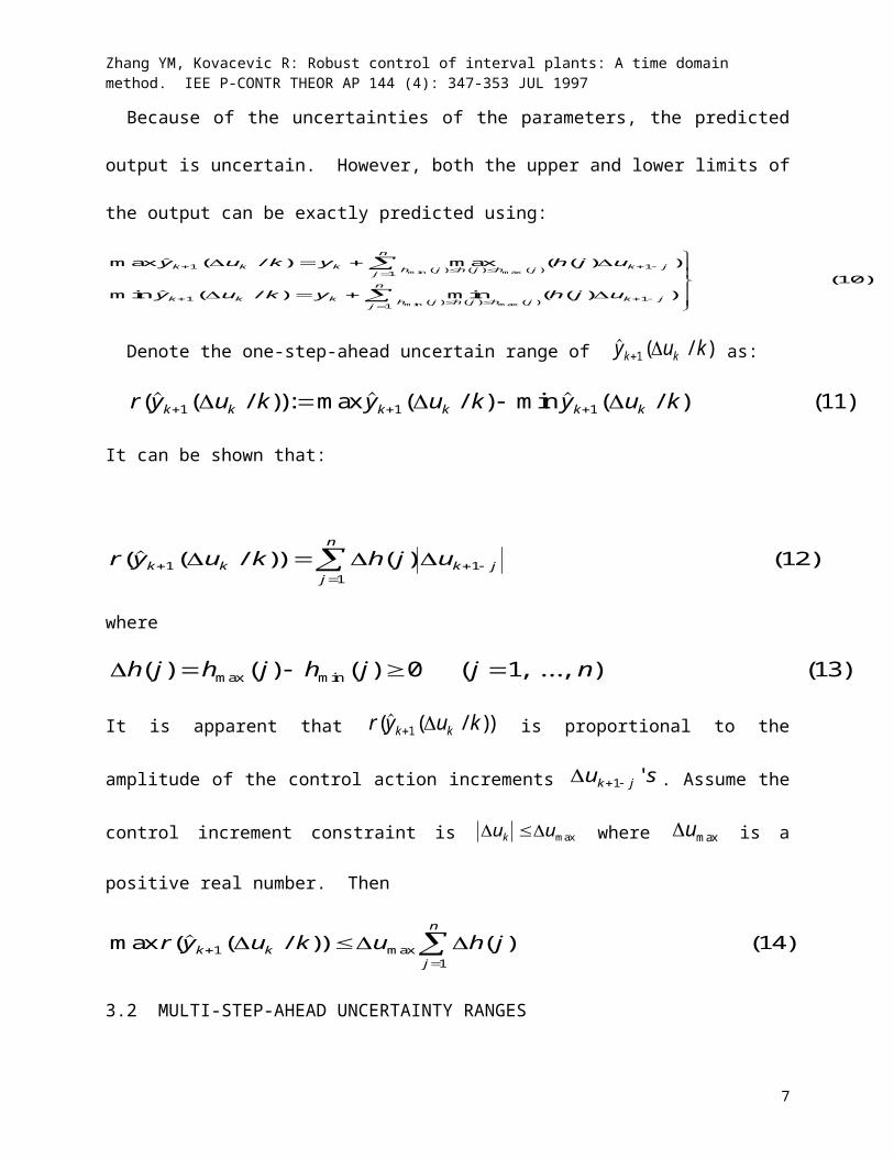
prediction based algorithm. Because of the uncertainty of the parameters in the interval model,

no exact predictions can be made. Hence, the predictions can only be given in certain ranges.

Consider instant k . Assume the feedback yk is available and uk needs to be determined.

From model (1), the following can be obtained:

y h j uk k jj

n

( ) (8)

1

where

y y yu u u

k k k

k j k j k j

1

1

3.1 ONE-STEP-AHEAD UNCERTAINTY RANGE

Based on Eq. (8), the following equation can be used as the prediction equation to predict the

output at instant k 1 :

( / ) ( )y u k y h j uk k k k jj

n

1 11

(9)

where k denotes the instant when the prediction is made, and uk gives the condition under

which the prediction is made. Here uk implies that all the previous and current u ’s are

known, i.e., uk j ’s are known for j 0 , when the prediction is made.

Because of the uncertainties of the parameters, the predicted output is uncertain. However,

both the upper and lower limits of the output can be exactly predicted using:

max ( / ) max ( ( ) )

min ( / ) min ( ( ) )

min max

min max

( ) ( ) ( )

( ) ( ) ( )

y u k y h j u

y u k y h j u

k k k h j h j h j k jj

n

k k k h j h j h j k jj

n

1 11

1 11

(10)

Denote the one-step-ahead uncertain range of ( / )y u kk k1 as:

r y u k y u k y u kk k k k k k( ( / )): max ( / ) min ( / ) 1 1 1 (11)

4


It can be shown that:

r y u k h j uk k k jj

n

( ( / )) ( )

1 11

(12)

where

h j h j h j j n( ) ( ) ( ) ( , ..., )max min 0 1 (13)

It is apparent that r y u kk k( ( / ))1 is proportional to the amplitude of the control action

increments u sk j 1 ' . Assume the control increment constraint is u uk max where umax is

a positive real number. Then

max ( ( / )) ( )maxr y u k u h jk kj

n

11

(14)

3.2 MULTI-STEP-AHEAD UNCERTAINTY RANGES

Based on the one-step-ahead prediction equation (9), the following recursive multi-step-ahead

prediction equation can be obtained:

( , , ... , / ) ( , , ... , / ) ( )y u u u k y u u u k h j uk i k i k i k k i k i k i k k i jj

n

1 2 1 2 31

(15)

where ( , , ... , / )y u u u kk i k i k i k 1 2 denotes the prediction of yk i made at instant k for the

known previous u ’s and assumed output u u uk i k i k 1 2, , ... , . Thus,

max ( , , ..., / )

max ( , , ..., / ) max ( ( ) )

min ( , , ..., / )

min ( , , ..., / ) min

min max( ) ( ) ( )

y u u u k

y u u u k h j u

y u u u k

y u u u k

k i k i k i k

k i k i k i k h j h j h j k i jj

n

k i k i k i k

k i k i k i k h

1 2

1 2 31

1 2

1 2 3

min max( ) ( ) ( )

( ( ) )

( ( , , ..., / ))

( ( , , ..., / )) ( )

( )j h j h j k i j

j

n

k i k i k i k

k i k i k i k k i jj

n

h j u

r y u u u k

r y u u u k h j u

i

1

1 2

1 2 31

2

(16)

That is, the maximum, minimum and uncertain range of the multi-step-ahead prediction can be

recursively calculated.

3.3 STEP RESPONSE PREDICTION

In the proposed algorithm, the control variable uk will be determined based on the output

behavior if the control variable remains at the current level, i.e., u u jk j k ( )0 . Hence,

5


the step response of the output needs to be predicted. Denote the prediction of the step response

as z u kk i k ( / ) :

z u k y u u u u k iz u k y

k i k k i k i k i k k

k k k

( / ): ( , , ... , , / ) ( )( / )

1 2 10 0 0 1

(17)

Thus,

z u k z u k h j u

z u k z u k h j u

z u k z u k h j u

r z u

k i k k i k k i jj i

n

k i k k i k h j h j h j k i jj i

n

k i k k i k h j h j h j k i jj i

n

k i

( / ) ( / ) ( )

max ( / ) max ( / ) max [ ( ) ]

min ( / ) min ( / ) min [ ( ) ]

( (

min max

min max

( ) ( ) ( )

( ) ( ) ( )

1

1

1

k k i k k i jj i

n

k r z u k h j u

i

/ )) ( ( / )) ( )

)

1

1

( (18)

Hence, for a given uk , the uncertain range of the step response can be recursively calculated as

i increases.

From the recursive equations (18), the following correlations can be obtained:

z u kz u k

z u kz u k

n i i l

z u kz u k

k i k

k i l k

k i k

k i l k

k i k

k i l k

( / )( / )

max ( / )max ( / )

, )

min ( / )min ( / )

1

1 1 0

1

(

(19)

It can be seen that the prediction error y z u kk k k 1 1( / ) will contribute to the further

prediction errors y z u k y z u kk i k i k k i k i k ( / ), min ( / ), and y z u kk i k i k max ( / ) where

i 2 . Thus, once the new feedback yk1 is acquired, the predictions ( z u k sk i k ( / )' ,

min ( / )'z u k sk i k , and max ( / )' ( )z u k s ik i k 2 ) can be replaced by more precise innovative

predictions ( z u k sk i k ( / )' 1 , min ( / )'z u k sk i k 1 , and max ( / )'z u k sk i k 1 ( )i 2 ) so

that the control action can be adjusted based on the new feedback, where

z u k z u k

z u k z u k i

z u k z u k

k i k k i k z u k y

k i k k i k z u k y

k i k k i k z u k y

k k k

k k k

k k k

( / ): ( / )

max ( / ): max ( / ) ( )

min ( / ): min ( / )

( )

( / )

( / )

( / )

1

1 2

1

20

1 1

1 1

1 1

Also, it can be shown that

z u k z u k s i uz u k z u k s i u iz u k z u k s i u

k i k k i k k

k i k k i k k

k i k k i k k

( / ) ( / ) ( )max ( / ) max ( / ) ( ) ( )min ( / ) min ( / ) ( )

( )max

min

1

1

1

1 21

Eq. (21) gives the correlation between z u kk i k ( / ) and z u kk i k ( / ) 1 . Here z u kk i k ( / ) 1

predicts what the output will be if the control variable is not changed. Based on the required

6


output, the ideal z u kk i k ( / ) which needs to be achieved by adjusting the control variable can

be known. Thus, the error in the output that the closed-loop control algorithm needs to eliminate

can be known and used to determine uk . A control criterion and algorithm can therefore be

proposed.

4. CONTROL ALGORITHM

The following criterion is proposed to determine uk :

max ( / )z u k yk n k 0 (22)

This criterion can be realized by the following steps:

(1) Calculate

max ( / ) ( ) ( )z u k n ik i k 1 1 23

based on (20) and (18).

(2) Because of the correlation in (21), calculate

d n y z u kk n k( ) max ( / ) 0 1 (24)

(3) Then

u d n s nk ( ) / ( )max (25)

5. PERFORMANCE

Theorem 1: For the given interval plant control problem (1), (3), and (7),

limk ky y

0 (26)

when algorithm (23-25) is used.

Proof: When the upper limit of the prediction is used to predict the output yk 1 at instant k , the

one-step-ahead prediction error defined by

e z u k yk k k k 1 1 1: max ( / ) (27)

7


is larger than or equal to zero, i.e. ek 1 0 . Based on Eqs. (19) and (20), the following can be

yielded:

max ( / ) max ( / ) , , ... )z u k z u k e ik i k k i k k 1 2 31 ( (28)

(In the journal, this equation was misprinted as

)

It is known that max ( / )z u k yk i k k i 1 and max ( / )z u k yk i k k i . Hence, Eq. (28) and

ek 1 0 imply that max ( / )z u kk i k 1 gives a more accurate prediction than max ( / )z u kk i k ,

and ek 1 0 is a measure of the prediction accuracy improvement when the new feedback yk 1 is

used for prediction.

In the following proving process, the correlation between uk 1 and ek 1 will be first

established. Then limk ku

0 will be shown based on ek 1 0 . As given by (25), uk ’s are

proportional to the differences between the set-point and predictions. Hence, limk ku

0 has

actually implied the correctness of (26).

Eq. (28) has the following form for i n 1:

max ( / ) max ( / )z u k z u k ek n k k n k k 1 1 11 (29)

Since

max ( / ) max ( / ) ( )z u k z u k ik i n k k n k (30)1

then

max ( / ) max ( / )z u k z u k e y ek n k k n k k k 1 1 0 11 = (31)

8


From (21) and (22), we have

max ( / ) max ( / ) ( ) ( )maxz u k z u k s n u yk n k k n k k 1 1 1 1 01 1 32

(Corrected:

)

Hence, also from (8),

u e s nk k 1 1 0/ ( )max (33)

(Corrected: Hence, . Because , Also,

. Thus, and . As a result,

u e s nk k 1 1 0/ ( )max (33) )

The control sequence satisfies:

u u uk k k 1 2 . ... (34)

Since the plant is stable and y yk i 0 , limi k iu 0 . In general, this can be written as

limk ku

0 (35)

Thus, from (16) it can be seen when k

max min ( ) ( )y y y ik i k i k 1 36

Also, since uk 0 when k ,

9


y y y kk n k n 1 1 0max ) ( (37)

That is,

limk ky y

0 ||

Remark 1: Theorem 1 shows that if (7) is satisfied, the proposed control algorithm can

guarantee that the required closed-loop system performance (4) is achieved. That is, the

resultant closed-loop system is robust with respect to the uncertainty of the interval plants in

achieving the closed-loop performance (4).

Remark 2: It can be seen from the above proof that the robust performance achieved by the

proposed algorithm is not affected by the dynamics of the controlled process such as open-loop

overshooting, delay, non-minimum phase, and large intervals once the sign condition is satisfied.

Remark 3: For the convenience of derivation, the algorithm has been developed using

impulse response function models. In general, a SISO interval plant can be described using an

autoregressive moving-average interval model:

y a j y b j uk k jj

p

k jj

q

= + (38)( ) ( )

1 1

where ( , )p q are the orders, and a j s j p( )' ( , ) ..., 1 and b j s j q( )' ( , ) ..., 1 are the real

coefficients of the model and satisfy:

a j a j a jb j b j b j

min max

min max

( ) ( ) ( )( ) ( ) ( )

(39)

In order to describe the interval plant (38) using the impulse response function model (1), one

can compute the responses of (38) to an impulse input uk k where 0 1 and k k 0 0 ( )

under zero initial state condition: y kk 0 0 ( ) . For convenience of notation, denote

b j b j b j j qmin max( ) ( ) ( ) ( ) 0

Thus, from (38), the following can be shown:

10


h k y a j y b k

h k y a j y b kk

k a j a j a jy y

k jj

p

b k b k b k

k a j a j a jy y

k jj

p

b k b k b k

k j k j

k j k j

max ( ) ( ) ( )min max

( ) ( ) ( )

min ( ) ( ) ( )min max

( ) ( ) ( )

( ) max max ( ) max ( )

( ) min min ( ) min ( ))

min max min max

min max min max

= +

= + ( (40)

1

1

1

Hence, { ( ), ( )}min maxh k h k ( )k 1 can be recursively calculated. We assume that the plant (38)

with interval parameters given in (39) is stable, and that the maximum and minimum of the

impulse responses approach to zero, i.e.,

lim ( )

lim ( )

max

min

k

k

h k

h k

0

0

so that the plant (38) can be described at any required accuracy by the interval impulse model

with a sufficient n . In this case, the interval (38) can be controlled using the proposed

algorithm.

Remark 4: Consider the case with disturbance:

y h k uk k j kj

n

( )

1

(1' )

where k is the disturbance at instant k . It can be shown that if l c l ( )1 where c is an

unknown (real) constant, then

limk ky y

0 (26)

when algorithm (23-25) is used. In fact, if k 1 , all the recursive equations in Section III still

hold so that the derivation in the proof of theorem 1 can be exactly repeated. This implies that

the robust performance for tracking a given set-point can also be obtained when the disturbance

is present.

Remark 5: The proposed control criterion is:

max ( / )z u k yk n k 0 (22)

If the criterion were

max ( / )z u k yk k 1 0 (27)

11


the resultant control would be similar to the one-step-ahead prediction based control. In this

case, the robustness of the resultant closed-loop performance is not guaranteed. In general, for

many interval plants, criterion

max ( / )z u k yk m k 0 (28)

may obtain the performance (4) with 1 m n . However, theoretical work which can be used to

judge whether an m (1 m n ) exists for guaranteeing the performance (4) for a given interval

plant has not been established in this paper. When an m (1 m n ) is used, the regulation speed

would improve when m decreases, whereas the robustness of the performance would tend to be

poorer.

6. SIMULATION

Example 1: Consider an interval plant family described by:

H

H

T

T

min

max

[ , ]

[ . , ]

0

0 2

0, 0, 0.9, 0.5, 0, - 0.3, - 0.5

0.2, 0.2, 1.3, 0.8, 0.2, - 0.1, - 0.3

Thus,

S

S

T

T

min

max

[ , ]

[ . , ]

0

0 2

0, 0, 0.9, 1.4, 1.4, 1.1, 0.6

0.4, 0.6, 1.9, 2.7, 2.9, 2.8, 2.5

Let y0 1 and k 0. When H H H H H min min max, ( ) / ,2 and H H H H min max min. ( )0 8 ,

the resultant closed-loop responses and control actions are plotted in Fig. 1(a)-(c), respectively.

It can be seen that both open-loop delay and overshooting exist in the plant. Despite the

significant uncertainties in the model parameters, stabilizing closed-loop control has been

achieved in all the cases.

Example 2: In this example, all the parameters are the same as in Example 1 except for the

disturbance. In this example, k 0 5. . The results are shown in Fig. 2.

Example 3: Consider a non-minimum phase interval plant family described by:

H

H

T

T

min

max

[ . , ]

[ . , ]

0 8

0 6

0.4, 0, 0.3, 0.9, 0.5, 0.3, 0.1, 0.2

0.2, 0.2 0.5, 1.3, 0.8, 0.5, 0.2, 0

12


Thus,

S

S

T

T

min

max

[ . , . , . , . , , . , . , . , . ]

[ . , . , . , . , , , , ]

0 8 12 1 2 0 9 0 0 5 0 8 0 9 0 7

0 6 0 8 0 6 0 1

1.2 2 2.5 2.7, 2.7

Let y0 1 and k 0. When H H H H H min min max, ( ) / ,2 and H H H H min max min. ( )0 8 ,

the resultant closed-loop responses and control actions are plotted in Fig. 3(a)-(c), respectively.

It can be seen that the plants are non-minimum phase and stabilizing closed-loop controls have

been obtained.

7. APPLICATION EXAMPLE

The proposed control algorithm has been applied to control the weld penetration. It is known

that weld penetration control is a major research issue in automated welding. The difficulty

arises from the invisibility of the weld penetration from the front-side. The present authors have

proposed to estimate the weld penetration by processing the image of the weld pool [24, 25].

The input and output of the controlled system are the welding current and the weld penetration

state, respectively. It is known that the process model varies with the welding conditions such as

the thickness of the material, etc. Hence, the interval model has been used for controller design.

The resultant interval model can be illustrated by hmin and hmax as shown in Fig. 4. Using this

interval model, a closed-loop system has been developed to control the weld penetration.

Extensive experiments have been done. As an example, Fig. 5 shows an experiment where

the travel speed changes from 2.0 mm/s to 3.0 mm/s. It can be seen that when the speed

increases, the output decreases (Fig. 5(a)). However, the controller can increase the current (Fig.

5(b)). As a result, the output is maintained at the desired level again (Fig. 5(a)). In this case, no

overshooting or fluctuation of the output occurs so that the geometrical regularity and

appearance of the resultant welds are excellent.

8. CONCLUSIONS

13


The interval plants described by given (1) and (3) can be controlled using the proposed

algorithm. The closed-loop control actions are directly determined from uncertainty ranges, i.e.,

the intervals, of the model parameters. Robust performance (4) is guaranteed if the sign

certainty condition (6) is satisfied, despite possible open-loop overshooting, delay, nonminimum

phase and large uncertainty intervals.

ACKNOWLEDGEMENT

This work is a part of the research for advanced control of material joining supported by the

National Science Foundation (DMI-9412637 and DMI-9419530) and Allison Engine Company,

Indianapolis, IN.

14


REFERENCES

[1] Chapellat, H., and Bhattacharyya, S. P., 1989. A generalization of Kharitonov’s theorem:

robust stability of interval plants. IEEE Transactions on Automatic Control, Vol. 34: 306-311.

[2] Barmish, B. R., et al., 1992. Extreme points results for robust stabilization of interval plants

with first order compensators. IEEE Transactions on Automatic Control, Vol. 37: 707-714.

[3] Barmish, B. R., and Kang, H. I., 1992. Extreme point results for robust stability of interval

plants: beyond first order compensater. Automatica, Vol. 28: 1169-1180.

[4] Dehleh, M., Tesi, A., and Vicino, A. 1993. An overview of extreme properties for robust

control of interval plants. Automatica, Vol. 29: 707-721.

[5] Barmish, B. R., and Kang. H. I., 1993. A survey of extreme point results for robustness of

control systems. Automatica, Vol. 29: 13-35.

[6] Shaw, J., and Jayasuriya, S., 1993. Robust stability of an interval plant with respect to a

convex region in the complex plane. IEEE Transactions on Automatic Control, Vol. 38:282-

287.

[7] Zhao, Y., and Jayasuriya, S., 1994. On the generation of QFT bounds for general interval

plants. ASME Journal of Dynamics Systems, Measurement, and Control, Vol. 116: 618-627.

[8] Foo, Y. K., and Soh, Y. C., 1994. Closed-loop hyperstability of interval plants. IEEE

Transactions on Automatic Control, Vol. 39: 151-154.

[9] Kogan, J., and Leizarowitz, 1995. Frequency domain criterion for robust stability of interval

time-delay systems. Automatica, Vol. 31: 462-469.

[10] Vicino, A., and Tesi, A., 1990. Regularity conditions for robust stability problems with

linearly structured perturbations. Proceedings of the 29th IEEE Conference on Decision and

Control, pp. 46-51, Honolulu, Hawaii, December 5-7.

15


[11] Abdallah, C., et al., 1995. Controller synthesis for a class of interval plants. Automatica,

Vol. 31: 341-343.

[12] Olbrot, A. W., and Nikodem, M., 1994. Robust stabilization: some extensions of the gain

margin maximization problem. IEEE Transactions on Automatic Control, Vol. 39: 652-657.

[13] Clarke, D. W., Mohtadi, C., and Tuffs, P. S., 1987. Generalized predictive control,

Automatica, Vol. 23: 137-160.

[14] Zhang, Y. M., Kovacevic, R., and Li, L., 1996. Adaptive control of full penetration GTA

welding. IEEE Transactions on Control Systems Technology, Vol. 4: 394-403.

[15] Campo, P. J. and Morari, M., 1987. Robust model predictive control. Proceedings of 1987

American Control Conference, pp. 1021-1026. Minneapolis, MN.

[16] Allwright, J. C. and Papavasiliou, G. C., 1992. On-linear programming and robust model-

predictive control using impulse-responses. Systems & Control Letters, Vol. 18: 159-164.

[17] Clarke, D. W., and Scattolini, R., 1991. Constrained receding-horizon predictive control.

IEE Proceedings, Part D: Control Theory and Applications, Vol. 138: 347-354.

[18] Kouvaritakis, B., Rossiter, J. A., and Chang, A. O. T., 1992. Stable generalized predictive

control: an algorithm with guaranteed stability. IEE Proceedings, Part D: Control Theory and

Applications, Vol. 139: 349-362.

[19] Kouvaritakis, B., and Rossiter, J. A., 1993. Multivariable stable generalized predictive

control. IEE Proceedings, Part D: Control Theory and Applications, Vol. 140: 364-372.

[20] Kovacevic, R., Zhang, Y. M., and Ruan, S., 1995. Sensing and control of weld pool

geometry for automated GTA welding. ASME Transactions Journal of Engineering for

Industry, Vol. 117: 210-222.

[21] Bidan, P., Boverie, S., and Chaumerliac, V., 1995. Nonlinear control of a spark-ignition

engine. IEEE Transactions on Control Systems Technology, Vol. 3: 4-13.

16


[22] Rajkumar, V., and Mohler, R. R., 1995. Non-linear control methods for power systems: a

comparison. IEEE Transactions on Control Systems Technology, Vol. 3: 231-237.

[23] Ling, K.-V., and Dexter, A. L., 1994. Expert control of air-conditioning plant.

Automatica, Vol. 30: 761-773.

[24] Kovacevic, R., and Zhang, Y. M., 1997. Neurofuzzy model-based weld fusion state

estimation. To appear in IEEE Control Systems Magazine, 17(2), April.

[25] Zhang, Y. M., Li, L., and Kovacevic, R., 1997. Dynamic estimation of full penetration

using geometry of adjacent weld pools. To appear in ASME Journal of Manufacturing Science

and Engineering, 119(2), May.

LIST OF ILLLUSTRATIONS

Fig. 1 Control of delay interval plants. (a) H H min , (b) H H H ( ) / ,min max 2 (c) H H H H min max min. ( )0 8 .

Fig. 2 Control of delay interval plants under constant disturbances. (a) H H min , (b) H H H ( ) / ,min max 2 (c) H H H H min max min. ( )0 8 .

Fig. 3 Control of non-minimum phase interval plants. (a) H H min , (b) H H H ( ) / ,min max 2 (c) H H H H min max min. ( )0 8 .

Fig. 4 Illustration of the identified interval model.

Fig. 5 Closed-loop experiment for controlling the weld penetration. (a) output (b) control action. A parametric perturbation is applied by increasing the welding speed from 2 mm/s to 3 mm/s at t s40 .

17


0 10 20 30 40 50 60 70 80 90100Discrete Time

00.20.40.60.8

11.21.41.61.8

y,u y

u

(a)

0 10 20 30 40 50Discrete Time

00.10.20.30.40.50.60.70.80.9

11.1

y,u

y

u

(b)


00.10.20.30.40.50.60.70.80.9

11.1

y,u

(c)

y

u

Fig. 1 Control of delay interval plants. (a) H H min , (b) H H H ( ) / ,min max 2 (c) H H H H min max min. ( )0 8 .

18


0 10 20 30 40 50 60 70 80 90100Discrete Time

0.20.30.40.50.60.70.80.9

1y,

u

yu

(a)


00.10.20.30.40.50.60.70.80.9

11.1

y,u

y

u(b)


00.10.20.30.40.50.60.70.80.9

11.1

y,u

(c)

y

u

Fig. 2 Control of delay interval plants under constant disturbances. (a) H H min , (b) H H H ( ) / ,min max 2 (c) H H H H min max min. ( )0 8 .

19


0 10 20 30 40 50 60 70 80 90100Discrete Time

-0.6-0.4-0.2

00.20.40.60.8

11.21.41.6

y,u

y

u

(a)


-0.4-0.2

00.20.40.60.8

1

y,u

yu

(b)


-0.4-0.2

00.20.40.60.8

1

y,u

(c)

y

u

Fig. 3 Control of non-minimum phase interval plants. (a) H H min , (b) H H H ( ) / ,min max 2 (c) H H H H min max min. ( )0 8 .

20


1 2 3 4 5 6 7 8 9 10 11 12 13 14 15 16 17 18 19 20

discrete time

00.010.020.030.040.050.060.070.08

h (m

m/A

)

hmaxhmin

Fig. 4 Illustration of the identified interval model

0 10 20 30 40 50 60 70 80time (second)

02468

1012

y (m

m)

(a)

0 10 20 30 40 50 60 70 80time (second)

405060708090

i (A

)

(b)

Fig. 5 Closed-loop experiment for controlling the weld penetration. (a) output (b) control action. A parametric perturbation is applied by increasing the welding speed from 2 mm/s to 3 mm/s at t s40 .

21

Documents

ROBUST CONTROL OF INTERVAL PLANTS: - …ymzhang/Papers/Interval Control Paper.doc · Web viewinterval model, predictive control, welding. 1. INTRODUCTION Interval models are useful