Embed Size (px)
Citation preview

Robust Control of Diesel Drivelines
Abdolreza Fallahi
A thesis submitted in partial fulfillment of the requirements of the University of East
London for the degree of
Doctor of Philosophy
May 2012

2
Acknowledgements
This research was inspired by my supervisor, Professor Stephen Dodds, whose valuable
technical support enabled its successful completion. This was complemented by much
encouragement on a personal level from Professor Dodds and his wife, Margaret,
without whom the journey would have been more difficult. I would also like to thank
my colleagues, A. Rawat, J. Pedersen and S. Kanchanavally, who also provided moral
support. I thank Dr W. Hosny for being my second supervisor. Also, I would like to
take this opportunity to thank my managers G. Forward, D. Higham and A. Potter. I
owe many thanks to Janet (my wife) and children.

3
Summary
The original contribution of this thesis is to provide insight into research of non-
traditional control techniques for automotive power train applications, culminating in
experimental evidence of much improved performance and reduced commissioning
costs. This includes much work on the technique of Observer Based Robust Control
(OBRC) which, before the research documented in this thesis commenced, was only in
its infancy with some promise being shown through the simulation of electric drive
applications (Dodds, 2007). The thesis, therefore, contributes to the process of bringing
this new control technique nearer maturity. OBRC is based on an observer designed to
provide information enabling effective control of an automotive power train application
and its performance assessment. Comparison with traditional and other robust control
techniques is included. The observer in OBRC is is designed to estimate the equivalent
disturbance input, referred to the control input to a plant. This represents plant
modelling errors as well as external disturbances. The equivalent disturbance estimate is
applied to the real plant input to cancel its effect, thereby reducing the control problem
to that of controlling the known real-time model of the plant employed in the observer.
One of the disadvantages of conventional robust control methods, such as those based
on sliding mode control, is that relatively high gain control loops are closed around the
uncertain plant. This increases the risk of instability due to the dynamic elements, such
as sensor lags, that are not included in the assumed plant model. The initial reason for
investigating OBRC is that the high gain loops are applied to the known plant model in
the observer and that the stability of these loops, taken in isolation, can therefore be
guaranteed. It was found that the observer gains are limited only by the finite sampling
frequency of the digital processor. In theory, infinite observer gains would yield ideal
robustness. However, in practice only finite gains are possible. The aforementioned
application of the equivalent disturbance estimate to the real plant input effectively
transfers the high gain loops from the plant model in the observer to the real plant. This
meant that closed loop stability could not be guaranteed under all circumstances. In
view of this, it was decided that sliding mode control should not be excluded from the

4
set of controllers for comparison. Since the control chatter associated with basic sliding
mode control has to be eliminated for the vehicle application, polynomial control (a
continuous version of the discrete RST controller) with robust pole assignment is
included. This polynomial control can be regarded as equivalent to the sliding mode
control with a boundary layer, but without the uncertainty associated with the choice of
the boundary layer width. Two more controllers, based on the Internal Model Control
(IMC) and H-infinity, are included for comparison on the basis that their design
methodologies do not demand high gains. The various control techniques are
demonstrated and compared via their application to Diesel Drivelines for commercial
road vehicles.
One of the operational problems with conventional PI engine speed controllers is the
need for time consuming initial controller tuning. This requires different sets of gains
for each gear selection, including idle (i.e., neutral) and later retuning to compensate for
changes in the driveline characteristics with component aging. A major advantage of
OBRC in this application is the elimination of the tuning procedure. Of particular
interest is the fact that the order of the system is increased by two when a gear is
engaged due to a vibration mode created by the finite torsional compliance of the
propeller shaft and other driveline components. Since this driven mechanical load can
be represented by its inverse dynamic model in a feedback path whose output acts at the
same point as the control variable, the OBRC compensates for this automatically
without the need for any parametric changes. The simulations and experimental work
were carried out on the DAF 12 litre diesel engine. The comparative study was carried
out, not only with respect to the main application of Diesel Drivelines, but also using
academic examples that are even more demanding of the controllers’ capabilities.
A key parameter in an engine configuration is the saturation limit on the injected fuel
rate, which is highly dependent on the engine capacity from 10 litres to 16 litres. One
example was introduced with a saturation block and the abilities of the various
controllers under this constraint were assessed. The H-infinity controller could not
handle such a saturation constraint, which is common practice in automotive

5
applications and therefore this had to deemed unsuitable. The remaining controllers
were able to operate with fuel rate saturation.
The overall conclusion is that the controllers based on OBRC, polynomial control and
IMC are capable of a similar performance with appropriate controller parameter
settings. However all are subject to the trade-off between the conflicting requirements
of short response times and robustness.
6
Contents
Acknowledgements ....................................................................... 2
Summary ....................................................................................... 3
List of Acronyms ........................................................................ 12
List of Figures ............................................................................. 13
1 Introduction ......................................................................... 17
1.1 Motivation for Research ............................................................................ 17
1.2 Original Contribution ................................................................................ 19
1.3 Overview of Engine Control ..................................................................... 20
1.4 Thesis structure ......................................................................................... 23
2 Essential Background and Definitions .............................. 25
2.1 Classical Control Loop Structure .............................................................. 25
2.2 Sensitivity Definition ................................................................................ 27
2.3 Robustness Definition ............................................................................... 28
2.4 Internal Stability Definition ...................................................................... 30
2.5 Control System Design Methodology ....................................................... 33
2.6 The Settling Time Formula ....................................................................... 35
3 Observer Based Engine Load Estimation ........................ 36
3.1 Overview ................................................................................................... 36
3.2 The Inverse Dynamic Load Representation .............................................. 37
3.3 Transfer Function for F(s) ......................................................................... 40
3.4 The Concept of Observer Based Load Estimation .................................... 43
3.5 The Observer and its Design ..................................................................... 45
3.6 Passenger Car Inverse Dynamic Simulation ............................................. 48
3.6.1 Overview ................................................................................................... 48
7
3.6.2 Observer Simulation Results ..................................................................... 49
3.6.3 Formulation of the unloaded Engine Model ............................................. 56
4 Observer Based Robust Control (OBRC): General Theory
............................................................................................... 60
4.1 Overview ................................................................................................... 60
4.2 The ‘plant model mismatch equivalent input’ premise ............................. 62
4.3 Formation of controller using the plant model mismatch equivalent input
63
4.4 Introduction of an Observer for the Estimation of External Disturbance . 64
4.5 Application to Diesel Engine Control ....................................................... 67
5 Comparison of Control Techniques for General
Applications ......................................................................... 70
5.1 Overview ................................................................................................... 70
5.2 Introduction to Other Control Techniques and their Design Procedures .. 70
5.3 OBRC Controller Design .......................................................................... 72
5.3.1 Overview ................................................................................................... 72
5.3.2 OBRC Model State Control Loop ............................................................. 72
5.3.3 Determining the OBRC Observer Gains ................................................... 75
5.3.4 Cascade Controller equivalent to OBRC .................................................. 76
5.4 The RST Controller [13, 36, 27, 37] ......................................................... 78
5.5 The Polynomial (RHF) Controller ............................................................ 79
5.5.1 Introduction ............................................................................................... 79
5.5.2 General Theory of the RHF Controller ..................................................... 80
5.5.3 Constraints on Polynomial Degrees .......................................................... 82
5.5.4 Sensitivity .................................................................................................. 83
8
5.5.5 Derivation of the General Pole Placement Equation ................................. 84
5.5.6 Basic RHF Controller Example ................................................................. 87
5.5.7 Example of RHF Controller with Integral Action ..................................... 88
5.5.8 Pre-compensator ........................................................................................ 90
5.5.9 Sine Wave Oscillator Example ................................................................. 90
5.6 The Internal Model Controller .................................................................. 92
5.6.1 Formulation of the IMC ............................................................................ 92
5.6.2 Sensitivity .................................................................................................. 94
5.6.3 Design Procedure ...................................................................................... 95
5.7 The H-Infinity Controller .......................................................................... 96
5.7.1 Overview ................................................................................................... 96
5.7.2 Formulation of the H-infinity Controller .................................................. 96
5.7.3 Design Specification ................................................................................. 97
5.7.4 Steps to use the Matlab Toolbox ............................................................... 99
5.8 Comparisons ............................................................................................ 100
5.8.1 Overview ................................................................................................. 100
5.8.2 Comparison of OBRC and H-infinity ..................................................... 100
5.8.3 Comparisons with Nominal Plant Model ................................................ 102
5.8.4 Comparisons with Parameter Variations ................................................. 112
5.8.5 Comparison of RHF and IMC Controllers .............................................. 112
5.8.6 Comparison of RHF and RST Controllers .............................................. 117
5.8.7 Summary ................................................................................................. 121
6. Comparison of Control Techniques for Engine Application
............................................................................................. 122
6.1 Overview ................................................................................................. 122
9
6.2 The OBRC Controller ............................................................................. 122
6.2.1 Overall Structure ..................................................................................... 122
6.2.2 Design of the OBRC Model Controller ................................................... 123
6.3 The IMC Controller ................................................................................. 125
6.3.1 Overall Structure ..................................................................................... 125
6.3.2 IMC Controller Design ............................................................................ 126
6.3.3 Simulations .............................................................................................. 128
6.4 Experimental Setup ................................................................................. 131
6.5 Comparison of Simulation Results and Test Results .............................. 132
7. Conclusions and Recommendations for Further Research
............................................................................................. 137
7.1 Conclusions ............................................................................................. 137
7.1.1 OBRC .................................................................................................... 137
7.1.2 Comparison of OBRC with Other Control Techniques ........................ 138
7.1.3 Engine Test ............................................................................................ 139
7.2 Overall Assessment ................................................................................. 139
7.3 Recommendations for Further Research ................................................. 140
A.1 Sensitivity Function .......................................................... 141
A.2Computer Aided Pole Assignment ................................................................ 143
A.2.1 Background ............................................................................................ 143
A2.2 Linear Characteristic Polynomial Interpolation ......................................... 143
A.2.3 Development of the LCPI Algorithm .................................................... 144
A.2.4 Summary of the steps of the numerical pole placement ........................ 148
procedure ............................................................................................................. 148
A.2.5 Matlab Script ......................................................................................... 149

10
A.2.6 Polynomial Coefficients ........................................................................ 153
REFERENCES ......................................................................... 163

11
List of Symbols
P Plant Transfer Function
G Plant Transfer Function
^ This symbol represents an Estimated Value
1z Time delay of One Sampling Period
K(s)
Compensator
C(s)
Compensator
S(s) Sensitivity Function
T(s) Complementary Sensitivity Function
n Positive Integer Indexing (0,1,…,n,)
u Control Signal
coT Time Constant
sT Settling Time
s Complex Variable of the Laplace Transforms
rl Road Load e.g. hills
vl Vehicle Load
rvl Sum of the rl and vl
ωb Bandwidth of System
fd Filter Time Constant for Derivative

12
List of Acronyms
OBRC Observer Based Robust Control
IMC Internal Model Control
EMS Engine Management System
SISO Single Input Single Output
RHF Transfer Function Blocks, R(s), H(s) and F(s) in continuous
polynomial control structure
RST Transfer Function Blocks, R(z), S(z) and T(z) in discrete polynomial
control structure
rpm Revolutions Per Minute
rad Radian
PID Proportional, Integral, Derivative
CAN Controller Area Network
PTO Power Take Off
LHP Left Half Plane
RHP Right Half Plane
SSE Steady State Error
ETC Electronic Traction Control
ABS Anti-lock Brake System
invy Inverse dynamics representation of vehicle model
stdy Vehicle model in standard form
13
List of Figures
Figure 1-1: Tractor of the Articulated Vehicle 18
Figure 1-2: Overview of a Diesel engine control structure 22
Figure 1-3: A typical working envelop of the diesel engine 23
Figure 2-1: SISO Linear Feedback Control System Block Diagram 25
Figure 2-22-2: SISO Linear Feedback Control System Block Diagram 27
Figure 2-3: Step response specification parameters 29
Figure 2-4: SISO Linear System Block Diagram for Internal Stability Analysis 31
Figure 3-1: Mathematical representation of the inverse dynamics 38
Figure 3-2: Pictorial representation of the inverse dynamics 39
Figure 3-3: Simplified block diagram of the vehicle with the dynamic engine load in the
inverse dynamic form 40
Figure 3-4: A first order plant and its model 43
Figure 3-5 Open loop block diagram of inverse dynamics and vehicle model with observer
49
Figure 3-6 Open loop speed response of inverse dynamic and standard models 50
Figure 3-7: Plot of the actual load, vl , and its estimate, vl , from the observer 51
Figure 3-8 Engine speed, vy , estimated engine speed, vy and external load torque 52
Figure 3-9: Standard and inverse dynamic vehicle models with proportional control loop
53
Figure 3-10: Plot of the estimated engine speed, vy , and the actual speed, vy , with a
cyclic external load torque, rl 54
Figure 3-11: plot of the estimated load and inverse dynamic load 55
14
Figure 3-12: Diesel Engine Block diagram with Physical Parameters 57
Figure 3-13: Block diagram of observer and unloaded engine 59
Figure 4-1: The plant model mismatch equivalent input 62
Figure 4-2: Plant model mismatch input cancellation 63
Figure 4-3: Controlling the uncertain real plant via control of the plant model 64
Figure 4-4: Introduction of an observer 65
Figure 5-1: OBRC closed loop system showing details of model state control loop 72
Figure 5-2: Model state control loop of OBRC for gain calculation 73
Figure 5-3: OBRC observer block diagram 75
Figure 5-4: OBRC and Hclosed loop response 77
Figure 5-5: General block diagram of SISO RST-Controller 78
Figure 5-6: General linear feedback SISO block diagram 79
Figure 5-7: General block diagram of SISO RHF-Controller 80
Figure 5-8 Simplified SISO block diagram of RHF-Controller for sensitivity analysis 83
Figure 5-9: Closed loop system for RHF design 87
Figure 5-10: Closed loop system for RHF design with integral action 88
Figure 5-11: General SISO block diagram for IMC 92
Figure 5-12: IMC block diagram with unity feedback 94
Figure 5-13 Block diagram of SISO IMC system 95
Figure 5-14: H-infinity Block diagram without constraints 96
Figure 5-15: H-infinity Block diagram showing constraint outputs 98
Figure 5-16: OBRC with low pass filtering in the error path without control saturation
100
Figure 5-17: OBRC with low pass filtering in the error path with control saturation 101
15
Figure 5-18: Frequency plot of filters with different time constants 101
Figure 5-19: Plot of the with lower filter gain 102
Figure 5-20: Effect of the higher gain filter on the error signal 103
Figure 5-21: OBRC and H-infinity step response with Controller effect 104
Figure 5-22: Step Response to change 15n (25% reduction) 105
Figure 5-23: Frequency plot of the closed loop system for OBRC and H-infinity 106
Figure 5-24: frequency plot of the K S OBRC with no error filtering and H-infinity 107
Figure 5-25: frequency plot of the 1 and 1S W for OBRC and H-infinity 108
Figure 5-26: Step response of the OBRC with no error filtering and H-infinity 108
Figure 5-27: Plot of the K S OBRC with error filtering and H-infinity 109
Figure 5-28: Step response of the OBRC with error filtering and H-infinity 110
Figure 5-29: Effects on S(s) when saturation is introduced at the Plant input 111
Figure 5-30: Further effects on |KS(s)| when saturation is introduced at the plant input
111
Figure 5-31: Plant parameter variations for robustness assessment 112
Figure 5-32: Bode plots of the uncontrolled plant for different parameter values 113
Figure 5-33: Step responses for the plant precisely matching the nominal plant model
114
Figure 5-34: Step response of RHF with model uncertainty 115
Figure 5-35: Step response of IMC with model uncertainty 115
Figure 5-36 Step response of RHF with pre-compensator 116
Figure 5-37 Step response of the RHF controller without pre-compensator 117
Figure 5-38: RFH with pre-compensator response to reference input
(sine(7t)+sine(5t)+ramp) 118
16
Figure 5-39: RFH without pre-compensator response to reference input
(sine(7t)+sine(5t)+ramp) 119
Figure 5-40: Error signal for RFH with pre-compensator 119
Figure 5-41: RFH with pre-compensator and RST response to reference input
(sine(16t)+sine(5t)+ramp) 120
Figure 5-42: Error for RFH with pre-compensator and RST 120
Figure 5-43: Plot of controller effort for RFH with pre-compensator and RST 121
Figure 6-1: Closed loop System block diagram for engine speed control 124
Figure 6-2 Closed loop block diagram incorporating IMC controller. 125
Figure 6-3 Closed loop block diagram of IMC structure with unity feedback 125
Figure 6-4: Basic IMC engine control loop 127
Figure 6-5: Derivative block with inbuilt low pass filtering 127
Figure 6-6: IMC engine control loop with pre-compensator 128
Figure 6-7: Step response of the IMC controller with pre-compensator 129
Figure 6-8: Further step response of the IMC Controller with pre-compensator 130
Figure 6-9: Step response of the IMC with and without pre-compensator 130
Figure 6-10 Experiment Setup 132
Figure 6-11 Comparison of simulated and test cell data 133
Figure 6-12 Comparison simulated torque and actual torque 134
Figure 6-13 Comparison of actual engine speed with simulated engine speed 135
Figure 6-14 Comparison of the torque and estimated 135
Figure 6-15: Plot of OBRC with and without external load signal 136
Figure A-1: Computer aided implementation tool for the LCPI method 144
Figure A-2: A computer aided method for calculating the desired characteristic
polynomial coefficients 145
17
1 Introduction
1.1 Motivation for Research
The aim of this research is to investigate control techniques that, in contrast with
traditional ones, do not require time consuming tuning procedures at commissioning
time together with subsequent and frequent retuning due to plant component ageing, and
to make recommendations for the future based on performance comparisons by
simulation and physical tests on an engine. A practical constraint is that the new control
algorithms can be implemented on currently available fixed point real time embedded
Micro-controllers with limited computation power. The investigation includes
comparison with presently implemented control techniques.
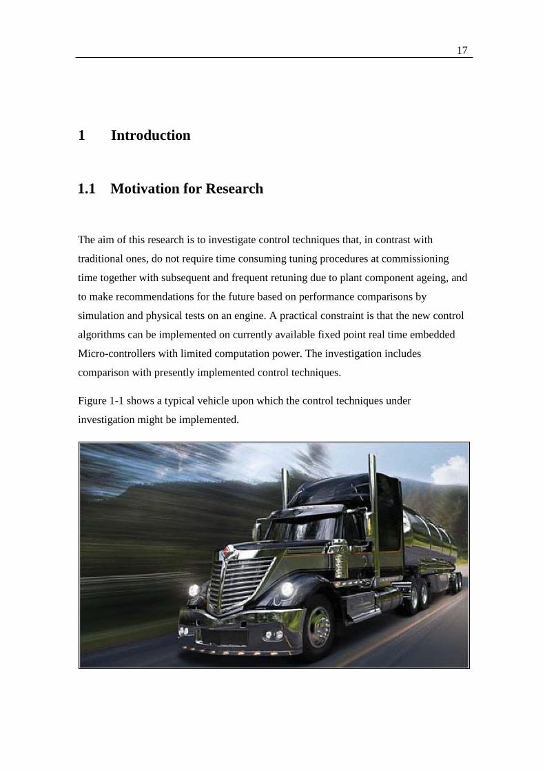
Figure 1-1 shows a typical vehicle upon which the control techniques under
investigation might be implemented.
18
Figure 1-1: Tractor of the Articulated Vehicle
The diesel engine controllers in the heavy duty sector (typically 10ltr to 16ltr) have been
controlled by 16 bit and 32 bit real time microprocessors, with fixed point capability
only. There is, however, a slowly developing trend towards floating point capability in
the new generation of microprocessors. The existing products, however, need to be
maintained and will require updates. This motivates the evolvement of improved control
techniques with minimal complexity.
The existing control algorithms that are run on the current products predominantly
implement PID (Proportional, Integral and Derivative) controllers. Although the PID
controller is linear in its basic form, non-linearities are commonly built into the
controllers for practical reasons. These nonlinearities vary in complexity, from simple
saturation on the actuator input and/or integral term anti-windup, to complex gain
scheduling based on the vehicle load and vehicle speed. There has been very little
change in the industry, as 95% of Engine Management Systems (EMS) are still using
PID controllers but control system improvements have evolved in the domain of the
gain scheduling. One reason for the PID controller continuing as the basic workhorse of
engine management systems is due to its track record of working reliably in various
applications, albeit with room for improvement in performance. The tuning however is
time consuming and has to be repeated during control system development and often at
service intervals. This is to compensate for the drift of the plant parameters, due to
component wear and ageing. Different vehicles may require different gains for a given
application. For example, if an application for a fire engine or a crane is used, then
different gains are required for the road speed controller. Hence one has to tune the
controller each time for a given application. The research programme is therefore directed
towards robust control techniques that avoid tuning and retuning. This will take advantage
of the digital implementation medium, particularly the future floating point processors, to
reach performance levels unattainable with PID controllers. The author initially developed
a road speed limiter with a PI controller [48], including nonlinear and variable gain
scheduling. The design had to cater for an empty vehicle (4,000kg), a fully loaded vehicle
(40,000kg) or a half empty fuel tanker truck. This also had to accommodate driveline

19
oscillation [51] and work with several different truck manufacturers. A DAF Truck
commission led a study into the robustness of the PI controller [48].
1.2 Original Contribution
The original contribution of this thesis is the assessment of the new OBRC control
technique, which is described fully in Chapter 4, together with three other control
approaches comprising polynomial control, IMC, described in Chapter 7 and H-
infinity, culminating in a recommendation of those that would be advantageous in
future engine speed control applications. The components of this original contribution
are as follows:
I: - The OBRC, which through its inherent robustness, ensures that the vehicle
speed follows a transient path which is prescribed by the control performance
specification, despite changes in the vehicle dynamics and external disturbances.
II: - The inverse dynamic method of estimating the model uncertainty (caused
by the un-modelled component of the plant and the external disturbance).
II: - Simplifying the modelling of a vehicle by means of the inverse dynamic
method and thereby reducing the required design effort in terms of man-hours,
when employing OBRC or polynomial control with robust pole placement.
IV: - The introduction of OBRC and polynomial control that eliminates tuning
of the controller in real time on the physical vehicle.
V:- A new numerical method for pole assignment.
VI:- A pre-filtering technique producing a prescribed transient behaviour..

20
1.3 Overview of Engine Control
The Diesel engine has been widely used as a power source in mass transportation.
Diesel engines are used in many applications such as articulated lorries, passenger
vehicles, medium duty vehicles, generator set prime movers and ship propulsion. The
capacity of these engines varies from 2.0 L up to 16L for mass transportation.
Most early engine speed control systems were based on mechanical governors which
were not flexible in terms of adjustable design parameters and consequently suffered
from compromised performance.
It is a well-known fact that the diesel engines are highly nonlinear plants and their
characteristics vary as function of power output, coolant temperature, oil pressure, oil
temperature, turbo charger characteristics and many other factors. The diesel engine
also renders the control system a discrete time one because the combustion occurs
every120 degrees of crankshaft rotation for a 6 cylinder, four stroke engine. In view of
the impulsive torque produced, the engine speed is filtered by a large flywheel.
Furthermore, a diesel engine is inherently open loop marginally stable in the sense that
the engine speed will drift away in the absence of closed loop control. Hence to prevent
the engine from running away or stalling, it requires a governor.
In general the engine control structure varies from company to company, such as Delphi
or Bosch. But they all have a basic structure which includes a strategy for starting the
engine, known as cranking, and a few other engine states such as running, idling,
cruising , PTO, etc.
The engine position and phasing is provided by two toothed wheels, usually mounted on
the engine flywheel and cam shaft. The cam shaft wheel teeth provide phasing of the
engine position and usually have N equally spaced teeth, where N is the number of
cylinders, plus one extra tooth that indicates cylinder 1 is approaching its compression
stroke. This wheel is known as an N+1 wheel. The flywheel teeth are more numerous,
usually being placed at intervals of 6 crank degrees spacing. This wheel would therefore
have 60 equally spaced teeth but 1 or 2 teeth are removed, to allow the system to run the
engine if the cam shaft sensor fails.

21
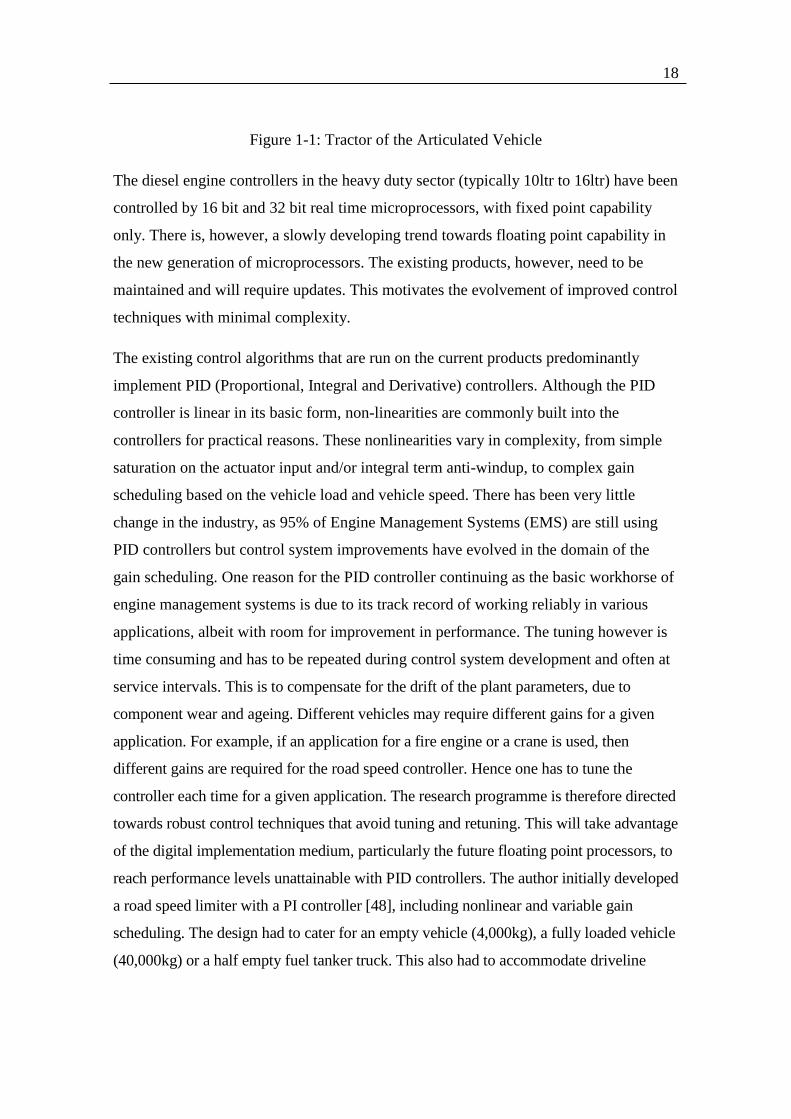
Figure 1.2 shows a typical structure of a Diesel engine control system whose functions
fall into one of the following two categories,
I: - Vehicle Control: Via the torque demanded by the driver (pedal, cruise
control via user interface, etc.) or via a CAN link which uses the J1939 standard,
and allows other devices (ABS, ETC, etc.) on the vehicle to control or limit the
engine torque.
II:- Engine Protection: A torque limit protects the engine against mechanical
and thermal damage. The full torque curve will protect the engine at the lower
end of the engine speed from mechanical damage and provides thermal
protection at the upper end. The maximum engine speed governor will protect
the engine from mechanical damage due to valve bounce and excessive internal
forces and torques due to component accelerations.
The smoke limiter prevents the engine from producing smoke due to incomplete
combustion by limiting the fuel quantity injected into the cylinder. The smoke limiter
becomes active during transient (change in load or step in speed demand,) and remains
active until the turbo charger catches up and provides the required air to the engine to
achieve complete combustion. During steady state operation, there is excess air in the
system, and therefore the smoke limiter is not active.
The idle speed governor prevents the engine from stalling and maintains the engine
speed when any auxiliary (power steering, air heater, etc) demands extra power.
22
Actual Torque
Driver Demand
Cruise Control
Full Torque Curve
PTO Governor
Road Speed Limiter
Maximum Speed
Governor
Smoke Limiter
Max
Min
Min
Idle Speed Governor
Torque Demand
Arbitration
Torque/Speed Control Message
Control Mode priority
Min
+
+
-
+
Accelerator Pedal
Mutually exclusive
Figure 1-2: Overview of a Diesel engine control structure
Figure 1.3 provides an overview of a typical engine operating envelope related to the
accelerator pedal position. Typical a pedal torque demand is a function of engine speed
and pedal position and is realised by means of a 3D lookup table. The lookup table is
used to create a proportional governor. It uses the line of constant pedal position against
engine speed and will reduce the pedal torque demand as the engine speed increases.
Some other applications may use the accelerator pedal position as the engine speed
demand (this is known as all speed governors) and this becomes a reference input to the
controller.

23
To
rqu
e [N
m]
Engine Speed [rpm]
Maxium Torque Curve
Zero Fuel Speed
Rated Speed
Idle Speed
Reference Point
Acce
lera
tor
Pe
da
l
Po
sitio
n [ %
]
Lines of Constant pedal
Position
Proportional governor for
high Idle Control
Isochronous governor for
high idle speed control
Figure 1-3: A typical working envelop of the diesel engine
1.4 Thesis structure
The thesis comprises of 6 chapters’, the content of which is as follows:
Chapter 1 provides a statement of the motivation for the research, a summary of the
original contributions and some background on engine management systems.
Chapter 2 provides the necessary background needed for understanding the material
of the subsequent chapters. It reviews the block diagram structure of the basic
control loop and its transfer function relationships, and defines the control system
properties of robustness, sensitivity and internal stability, discusses control system
design methodology and finally introduces the settling time formula as a simple
design tool for realising transient response specifications for control systems of
arbitrary order.
24
Chapter 3 first introduces a special form of observer for estimation of the external
disturbance referred to the control input and goes on to show that in the absence of
an external disturbance, this estimate enables plant parametric errors to be corrected,
and furthermore that if only a portion of the plant is modelled in the observer that the
disturbance estimate contains information about the remainder of the plant
represented in the inverse dynamic form. The application to a Diesel driveline is
considered. Finally, some preliminary experimental results and corresponding
simulations are presented of control of an engine subject to electromagnetically
generated load torques from a dynamometer, including the special observer and use
of the load torque estimate as part of the control signal to counteract the real load
torque.
Chapter 4 develops the observer based load estimation of Chapter 3 into the general
OBRC robust control technique as this is one of the original contributions of this
research programme to the field of engine management systems.
Chapter 5 introduces the control techniques to be compared with one another and
with the OBRC of Chapter 4 and then carries out the comparisons by analysis and
simulation using various plant examples.
Chapter 6 contains the comparisons of the control techniques by simulation and
experiment specifically for the Diesel driveline application.
Chapter 7 presents the conclusion of the thesis and recommendations for further
research.
The Appendix provides some supporting theory of the control techniques and some
design software.
25
2 Essential Background and Definitions
2.1 Classical Control Loop Structure
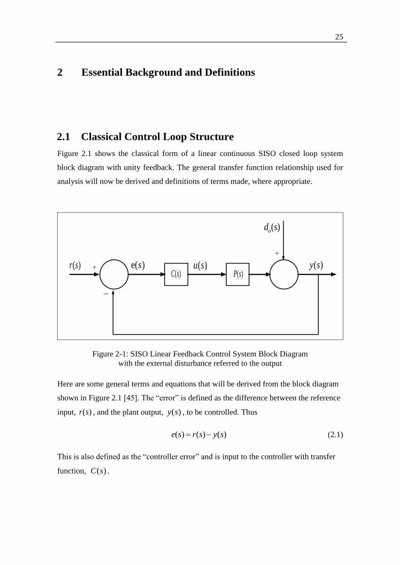
Figure 2.1 shows the classical form of a linear continuous SISO closed loop system
block diagram with unity feedback. The general transfer function relationship used for
analysis will now be derived and definitions of terms made, where appropriate.
( )r s e( )s( )C s ( )P s
( )u s ( )y s
( )od s
Figure 2-1: SISO Linear Feedback Control System Block Diagram
with the external disturbance referred to the output
Here are some general terms and equations that will be derived from the block diagram
shown in Figure 2.1 [45]. The “error” is defined as the difference between the reference
input, ( )r s , and the plant output, ( )y s , to be controlled. Thus
( ) ( ) ( )e s r s y s (2.1)
This is also defined as the “controller error” and is input to the controller with transfer
function, ( )C s .
26
The output of the controller ( )u s is then given by.
( ) ( )e( )u s C s s (2.2)
The external disturbance, ( )od s , is referred to the controlled output in Figure 2-1,
which is typical in the formulation of control loops designed by H methodology [9,
32]. Thus
( ) ( ) ( ) ( )oy s P s u s d s (2.3)
By substituting for ( )u s using (2.2) and (2.1), the closed loop transfer function
relationship may be derived as follows:
( ) ( ) ( ) ( ) ( ) ( )oy s P s C s r s y s d s (2.4)
( ) 1 ( ) ( ) ( ) ( ) ( ) ( )oy s C s P s C s P s r s d s (2.5)
Hence,
( ) ( )
( ) ( ) 1( ) ( ) ( )
1 ( ) ( ) 1 ( ) ( )o
T s S s
C s P sy s r s d s
C s P s C s P s
(2.6)
where T(s) is the closed loop transfer function and ( )S s is known as the sensitivity
transfer function. It should be noted that this provides a measure of the effect of the
external disturbance n the output. For further details, the derivation of the sensitivity can
be found in Appendix I A.1.1.
The loop transfer function is defined as ( ) ( ) ( )L s C s P s for the unity feedback system
as shown in Figure (2-1).
By inspection of (2.6),
( ) ( ) 1T s S s (2.7)
Hence ( )T s is sometimes referred to as the complementary sensitivity function.

27
2.2 Sensitivity Definition
Sensitivity is the proportional change in the closed loop transfer function divided by the
proportional change in the open loop transfer function. For analysis of the robust control
techniques other than H , the external disturbance, ( )id s , is referred to the control
input, as shown in Figure 2-2.
( )r s e( )s( )C s ( )P s
( )u s ( )y s
( )nu s
( )id s
Figure 2-22-2: SISO Linear Feedback Control System Block Diagram
with the external disturbance referred to the control input
In this case, the sensitivity, ( )S s , given in (2.6) is also the transfer function between
the external disturbance, ( )id s , and the net plant input, , ( )nu s , as shown in Figure 2.2.
In the frequency domain, the sensitivity is the Bode magnitude plot,
dB 1020logS S j . Then an upper threshold boundary, dBmaxS , is specified
for dBS . The specification is satisfied if dB dBminS S .
A typical control system specification including sensitivity could be as follows:
1. b The minimum bandwidth criteria (disturbance rejection).
2. The maximum peak of |S (jω)|.
3. The steady state error of the closed loop system.
28
2.3 Robustness Definition
There are several quantitative definitions for the robustness of a control system. Each
definition has an emphasis on a different aspect of the closed loop behaviour. In general,
however, it is defined qualitatively as its ability to maintain the specified closed loop
performance within given limits in the presence of an external disturbance and
modelling uncertainties due to plant wear over its operating life. Quantitative definitions
are made in the time domain [1, 45] and in the frequency domain [43]
One definition of robustness in the complex frequency ( )s domain is the
complementary sensitivity function, ( )T s , of (2.6). It is reasonable to suppose that as
the sensitivity reduces, the robustness increases, and this is certainly the case according
to (2.7). In the frequency domain, this may be a Bode magnitude plot,
dB 1020logT T j . Then a lower threshold boundary, dBminT , is specified
for dBT . The specification is satisfied if dB dBminT T over the frequency
range that the control system is required to operate. Usually, b0 , where b is
the control system bandwidth defined as the lowest angular frequency at which dBT
falls below dB 0T by 3 dB .
Maintenance of robustness in the frequency domain, however, does not imply that a
given transient response specification is satisfied. One way of assessing this
requirement is to examine variations of the step response with respect to the specified
one that result from the plant parameters being changed. The robustness can then be
defined as how little the step response changes with respect to the specified step
response for given plant parameter changes.
Care must be taken to specify a sufficient number of parameters of the step response.
For example, specifying the settling time alone according to the 5% criterion would be
insufficient because of the many different shaped step responses that are possible which
will have the same settling time. Some of these responses would be unacceptable due to
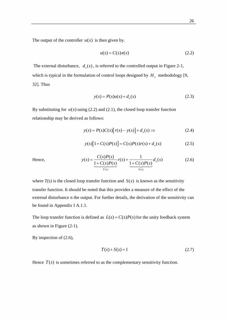
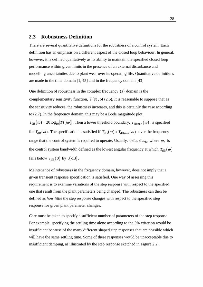
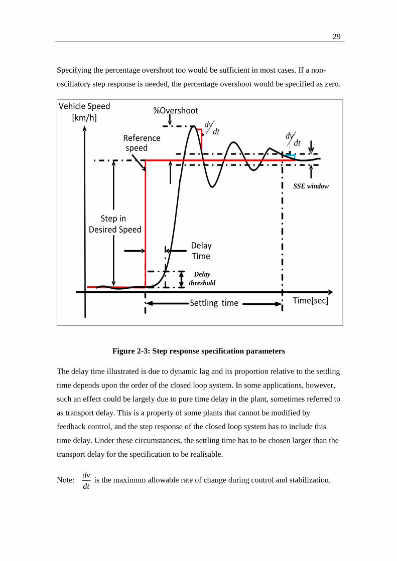
insufficient damping, as illustrated by the step response sketched in Figure 2.2.
29
Specifying the percentage overshoot too would be sufficient in most cases. If a non-
oscillatory step response is needed, the percentage overshoot would be specified as zero.
Time[sec]
dvdt
Vehicle Speed [km/h]
SSE window
dvdt
Step in Desired Speed
Reference speed
Settling time
%Overshoot
Time Delay
Delay
threshold
Figure 2-3: Step response specification parameters
The delay time illustrated is due to dynamic lag and its proportion relative to the settling
time depends upon the order of the closed loop system. In some applications, however,
such an effect could be largely due to pure time delay in the plant, sometimes referred to
as transport delay. This is a property of some plants that cannot be modified by
feedback control, and the step response of the closed loop system has to include this
time delay. Under these circumstances, the settling time has to be chosen larger than the
transport delay for the specification to be realisable.
Note: dv
dt is the maximum allowable rate of change during control and stabilization.
30
2.4 Internal Stability Definition
If a closed loop system is internally stable, it contains no unstable modes. The reason
for introducing this topic is that it is possible to find closed loop systems that appear to
be stable through having closed loop transfer functions with poles in the left half of the
s-plane, but are, in fact, unstable due to the cancellation of zeros in the right half of the
s-plane by closed loop poles in the same locations. In theory this could occur in a
controller designed by pole assignment but the control system designer would be aware
of the right half plane (RHP) zeros and would never attempt to cancel them. On the
other hand, the RHP zeros may be overlooked when using a sliding mode controller
with a boundary layer, the design of which only requires knowledge of the plant relative
degree [64, 65]. A similar issue could potentially occur with the observer based robust
control (OBRC) of Chapter 4. As the width of the boundary layer is reduced in the
sliding mode control, then this is equivalent to increasing the proportional gain in a unit
feedback control loop, so root loci of the system closely approach any RHP zeros,
causing instability. The unstable mode caused is internal in the sense that it cannot be
detected by observing the output response to the reference input. The system could then
be described as internally unstable.
A closed loop system that is internally stable is one whose characteristic equation has
roots with negative real parts. This is the characteristic equation of the system matrix of
the state space model of the closed loop system. Thus internal stability ensures that
there are no unstable modes of the closed loop system, whether or not they can be
detected by observing the output response to the reference input. It follows from the
above that a feedback control system is internally stable if it appears to be stable by
observing the output and reference input and there is no RHP pole zero cancellation.
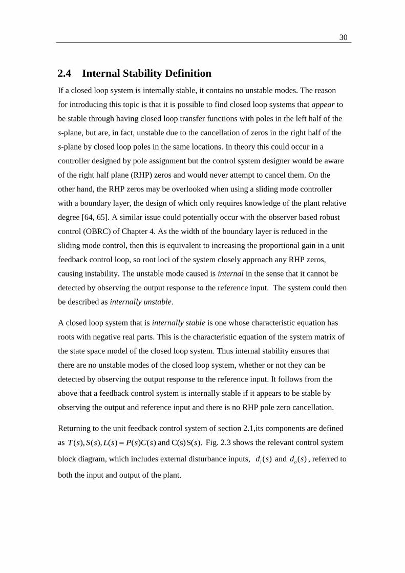
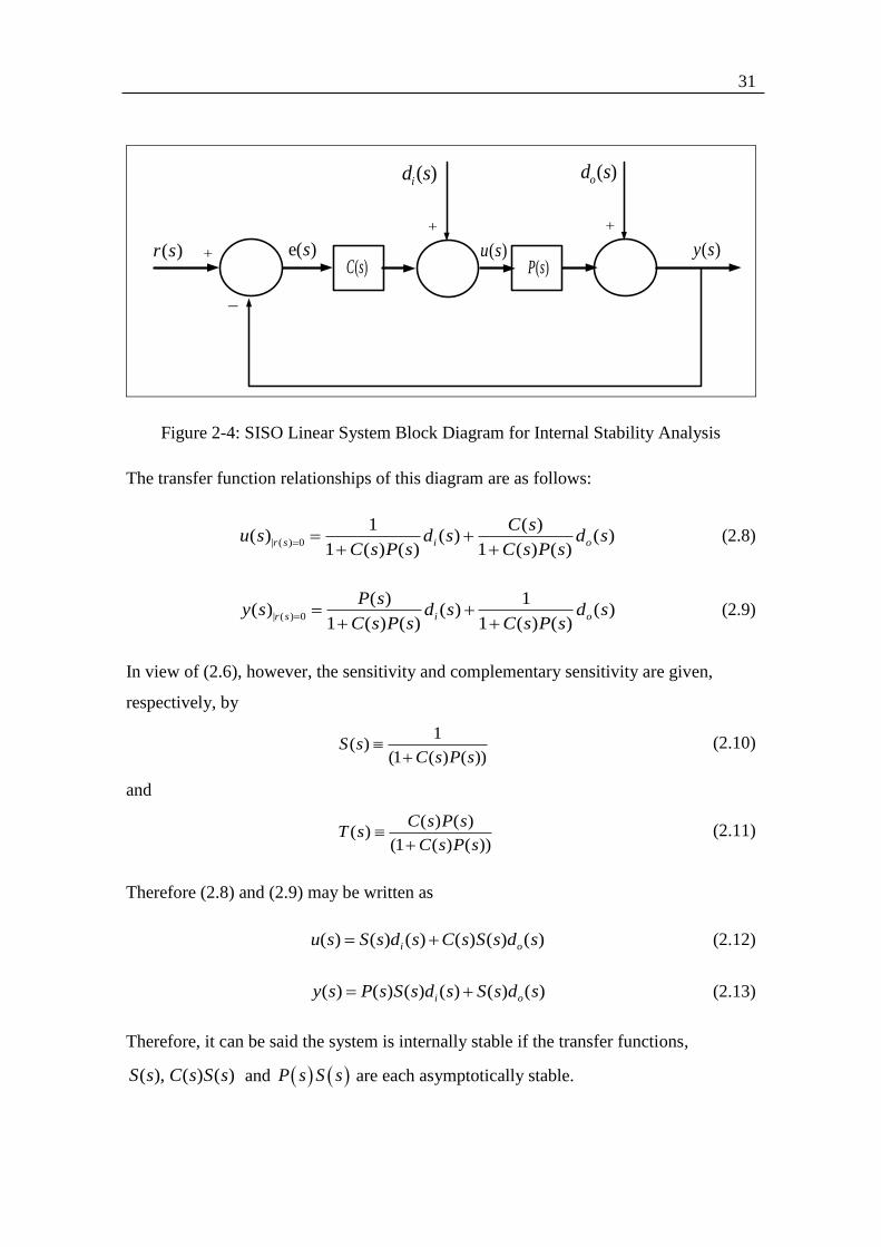
Returning to the unit feedback control system of section 2.1,its components are defined
as ( ), ( ), ( ) ( ) ( ) and C(s)S( ).T s S s L s P s C s s Fig. 2.3 shows the relevant control system
block diagram, which includes external disturbance inputs, ( )id s and ( )od s , referred to
both the input and output of the plant.
31
( )r s e( )s( )C s ( )P s
( )u s ( )y s
( )id s ( )od s
Figure 2-4: SISO Linear System Block Diagram for Internal Stability Analysis
The transfer function relationships of this diagram are as follows:
| ( ) 0
1 ( )( ) ( ) ( )
1 ( ) ( ) 1 ( ) ( )r s i o
C su s d s d s
C s P s C s P s
(2.8)
| ( ) 0
( ) 1( ) ( ) ( )
1 ( ) ( ) 1 ( ) ( )r s i o
P sy s d s d s
C s P s C s P s
(2.9)
In view of (2.6), however, the sensitivity and complementary sensitivity are given,
respectively, by
1( )
(1 ( ) ( ))S s
C s P s
(2.10)
and
( ) ( )( )
(1 ( ) ( ))
C s P sT s
C s P s
(2.11)
Therefore (2.8) and (2.9) may be written as
( ) ( ) ( ) ( ) ( ) ( )i ou s S s d s C s S s d s (2.12)
( ) ( ) ( ) ( ) ( ) ( )i oy s P s S s d s S s d s (2.13)
Therefore, it can be said the system is internally stable if the transfer functions,
( ), ( ) ( )S s C s S s and P s S s are each asymptotically stable.
32
By using an example, the meaning of an internally stable system can be shown clearly.
Consider a plant with transfer function given by
1
( )( 1)( 2)
P ss s
(2.14)
and its controller given by
( )
( )( )
s aC s
s b
(2.15)
The unity feedback structure of Figure 2-3 is assumed. Therefore, the open loop transfer
function is given by
( )
( ) ( ) ( )( 1)( 2)( )
s aL s P s C s
s s s b
(2.16)
Clearly, the RHP pole-zero cancellation is avoided if 1a in the controller design.
There is no cancellation of the RHP zeros or poles and therefore, the RHP pole remains
in ( )L s . The sensitivity transfer function is given by equation 2.10 and can be written
for the closed loop of the plant. Thus
1 1 ( )( 1)( 2)( )
( ) 11 ( ) ( ) ( )( 1)( 2) ( )1 .( ) ( 1)( 2)
s b s sS s
s aC s P s s b s s s a
s b s s
(2.17)
It can be seen that there is no pole zero cancellation if 1a .Next,
( ) ( )( 1)( 2) ( )( 1)( 2)( ) ( ) .
( ) ( )( 1)( 2) ( ) ( )( 1)( 2) ( )
s a s b s s s a s sC s S s
s b s b s s s a s b s s s a
(2.18)
Again, there is no pole-zero cancellation if 1a . Finally
1 ( )( 1)( 2)
.( 1)( 2) ( )( 1)( 2) ( )
P ss b s s
s s s bS s
s s s a
( )
( )( 1)( 2) ( )
s b
s b s s s a
(2.19)
This component would be unstable with 1a because ( 1)s , would become a factor
of the denominator. The conclusion of this analysis is that the control system designer

33
would be free to try and find values of c and 1a yielding internal stability by
forcing all three closed loop poles to be in the left half of the s-plane. It is important to
realise, however, that as it stands, the controller only has two adjustable parameters, c
and a , and therefore design by pole assignment, in which all three closed loop poles
can be chosen at the outset to achieve a specified transient response, cannot be done.
This problem could be solved, however, by introducing a proportional gain, K , in the
controller, so that ( )
( )( )
s aC s K
s b
.
2.5 Control System Design Methodology
Assuming that the plant, the controller and therefore the closed loop system are linear,
there are three basic control system design methodologies, as follows,
I: - Pole assignment to achieve a specified closed loop transient response. The
settling time formula of section 2.6 renders this methodology straightforward for
a linear plant of arbitrary order.
II: - Optimal control [51, 52, 63, 42], meaning the use of an optimisation
technique to determine the controller gains that minimise (or maximise) a given
cost function while respecting a set of constraints.
III: - Determination of the controller gains basically by tuning in real time on the
real plant but often proceeded by tuning using a simulation [46, 45].
Methodologies I and II are model based Methodology I is carried out in the time domain
but methodology II may be carried out in the time domain or the frequency domain.
The IMC, OBRC and the RFH controllers are compatible with design methodology I for
plants of any order. This is also true of the linear state feedback controller [1, 48,59].
The standard PID controller and its variants, i.e., the PI, PD, P (proportional) and
similar controllers of slightly different structure, are also compatible with design
methodology I but only for plants of limited order (second order for the PID and PD
controllers and first order for the PI and P controllers).
34
The H-infinity design approach applies to the design of a control system with the
classical unit feedback structure and is an example of methodology II in the frequency
domain [9, 23, 32, 40, 41, 43, and 50]. Formulating constraints for the H-infinity
method is an important part of the design process, since the optimisation tools will
exploit the weakness in ill-defined constraints and consequently the solution will not be
a robust one. Also, the H-infinity approach is most effective in assuring closed loop
stability in cases of extreme plant model uncertainty. The order of the resulting
controller, ( )C s , depends on the plant transfer function and the optimisation criterion.
The RST controller has a different structure and is another example of methodology II
in the frequency domain [26, 35, and 36]. Both of these require an optimisation tool in
order to design the controller.
The linear state feedback controller is also compatible with design methodology II in
the time domain when the gains are determined by the LQ method. Here, the plant state
space model and the weighting parameters of a linear quadratic integral cost function
are used in a matrix Ricatti equation to calculate the state feedback gains that minimise
the integral cost function [27, 66].
The standard PID controller and its variants are the only controllers lending themselves
to design methodology III but a plant model is not required. The tuning is essentially on
the basis of experience with specific types of plant but, with a new plant, has initially to
be by trial and error to build up the experience. It is important to note that this process
increases considerably in difficulty as the plant order increases beyond three and it may
be impossible in some cases to achieve a specified performance, in which case the more
sophisticated control techniques referred to above have to be considered.
Integral anti-windup is strongly recommended for any controller containing integral
terms to minimised issues due to control saturation. Also, and software differentiation
with inbuilt Measurement noise filtering is recommended in any controller requiring a
differential term to avoid momentary control saturation.

35
2.6 The Settling Time Formula
The Dodds settling time formula [46] is a means of control system design by pole
assignment to achieve a specified settling time with zero overshoot for a linear control
system of arbitrary order. For working with this formula, the settling time is defined as
the time taken to nominally reach the steady state value from one reference input level
to another either from a step up or a step down, noting that the transient response of any
continuous linear system takes an infinite time to reach a constant steady state value.
According to the 5% criterion, for a closed loop system with a unity closed loop DC
gain, it is the time taken for the magnitude of the error, ( ) ( ) ( )e t r t y t to fall to and
thereafter remain below 5% of its peak value. This time is measured from the instant at
which the peak occurs. If the poles of the closed loop system are made approximately
coincident at 1,2,..., 1/n cs T , where cT is the time constant of the n identical first order
subsystems connected in a chain to give the desired closed loop transfer function,
1
1
n
c
Y s
R s sT
(2.20)
The settling time formula provides a fairly accurate response up to a 6th order system
and can be easily corrected in one step to be applicable to systems of higher order than
this. The 5% formula is as follows:
1.5(1 )s cT n T (2.21)
where n is the order of the closed loop system. In view of equation (2.19), the desired
closed loop pole locations can be expressed in terms of sT and n as follows:
1,2,..., 1/ 1.5( 1) /n c ss T n T (2.22)
Hence, the general characteristic equation for the pole placement is given by
1.5( 1)
0
n
s
ns
T
(2.23)
36
3 Observer Based Engine Load Estimation
3.1 Overview
The aim is to estimate an external disturbance applied to a plant, with a view to
enhancing its control. Today’s production does not have a sensor to measure the torque
at the engine flywheel. Hence, the torque signal used in the system is estimated by
calibrating a series of lookup tables using empirical methods. This is done under the
steady state condition, ( , ,...)Torque f fuel Enginespeed . The alternative method
presented in this thesis is novel with respect to the field of road vehicle control. The
uniqueness of the method will be explained in this chapter.
In general, an observer [5, 49, 28] is designed to estimate the state of a plant in cases
where the state variables are required for use in a state feedback control law but cannot
be measured. This uses a plant model that matches the real plant as closely as possible.
The term, ‘state observer’ is used frequently in the literature but is really misleading as
it is not the state that is observed, since it is not available. Otherwise, the observer
would not be needed. It is actually the available signals that are observed, i.e., the plant
control variable, ( )u t , and the measurement variable, ( )y t . The term, ‘observer,’ comes
from the property of observability that a plant must have for it to be possible to estimate
the state, ( )tx . If a plant is observable, then, with the aid of an accurate state space
model of the plant, it is possible to estimate the present plant state, ( )tx , using past
observations of ( )u and ( )y , 0 t . In view of the above, the author prefers the
term “estimator,” to, “observer2,” but the terms may be used interchangeably. In fact,
the term “state estimator,” is also used instead of, “observer,” in the literature.
In the field of electric drives, an observer is often extended to be able to estimate an
external disturbance, ( )d t , referred to the control input, as well as the plant state [48].
Here, this idea is extended further to enable an observer to work with a greatly
simplified plant model that is not necessarily well matched to the real plant. It is this
type of observer that is employed in the OBRC fully described in Chapter 4. Such an
observer will be developed for application to a heavy duty vehicle later on in this,
37
chapter. In preparation for this, the vehicle, model hitherto referred to as the plant
model, will be fully discussed.
The plant is composed of several components comprising the engine, gearbox, drive
shaft, differential and the vehicle mass. There is also a considerable external disturbance
consisting of the gravitational force acting on the vehicle due to its inclination about the
pitch axis. This can be regarded as
a relatively complex system [26, 25]. The simplified model to be used in the estimator,
however, does not have to contain details such as the different gear ratios that may be
selected, the mass of the payload or the gravitational load force. This is because the
combined effect of all of these is equivalent to an external load torque applied to the
flywheel of the engine. An estimate of this equivalent external load torque and its
counteraction by a controller will be sufficient to handle all the aforementioned physical
influences. Hence, the simplified model consists just of the engine alone (disengaged
from the drive line).
3.2 The Inverse Dynamic Load Representation
The dynamics of a mechanical system model is defined as the part that yields rotational
and/or translational velocities when forces and/or torques are applied. The definition of
the inverse dynamics then follows naturally as a reformulation of the dynamics as the
part of the model that yields the forces and/or torques needed to produce given
translational and/or rotational velocities. The plant model will be divided into the
following two parts:
1) The dynamics model of the unloaded diesel engine
2) The inverse dynamics model of the remainder of the vehicle
A typical unloaded diesel engine can be represented by the transfer function of a first
order lag. Hence part (1) of the plant model is:
( )
( )( ) ( )
ve
y s bG s
u s s a
(3.1)
38
where ( )u s is the throttle input, i.e., the fuel volume flow rate, but this is scaled to be
numerically equal to the torque developed by the engine. ( )vy s is the measurement of
the flywheel speed. The constant parameters, a and b , are determined from
identification tests on the engine.
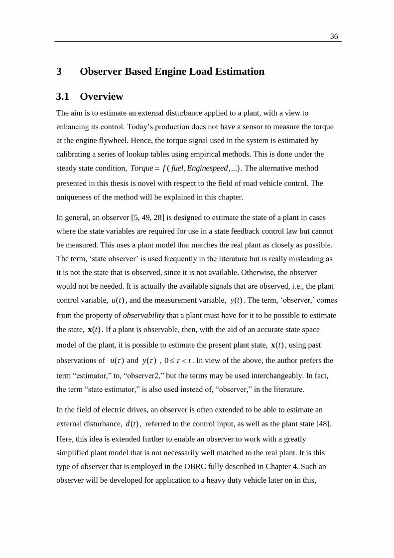
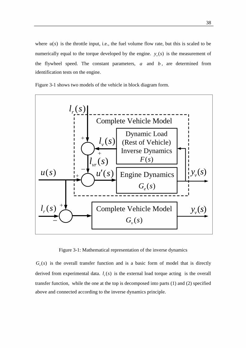
Figure 3-1 shows two models of the vehicle in block diagram form.
Complete Vehicle Model
( )vG s
( )vy s( )u s
( )rl s
( )rl s
( )vrl s
( )u s
( )vl s
Engine Dynamics
( )eG s
Dynamic Load
(Rest of Vehicle)
Inverse Dynamics
( )F s
Complete Vehicle Model
( )vy s
Figure 3-1: Mathematical representation of the inverse dynamics
( )vG s is the overall transfer function and is a basic form of model that is directly
derived from experimental data. ( )rl s is the external load torque acting is the overall
transfer function, while the one at the top is decomposed into parts (1) and (2) specified
above and connected according to the inverse dynamics principle.
39
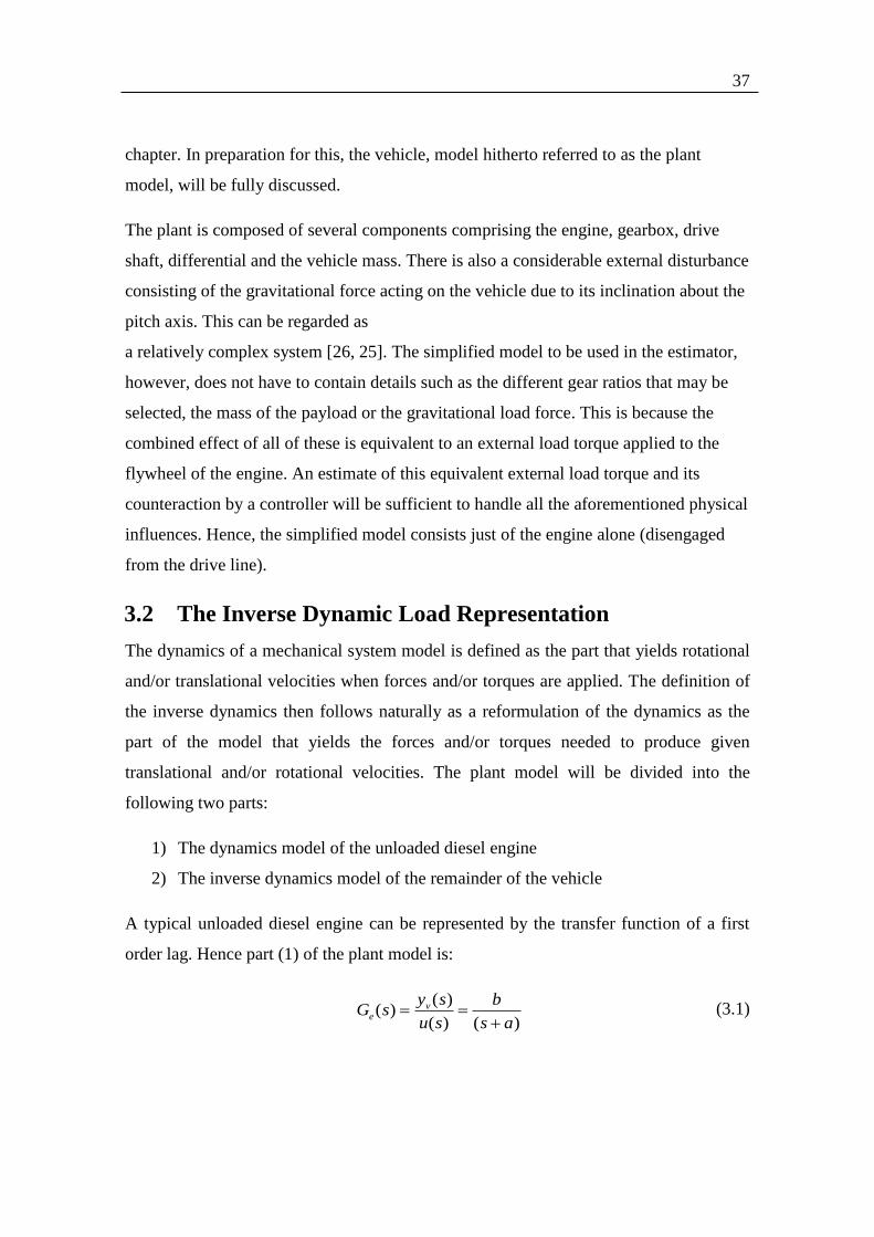
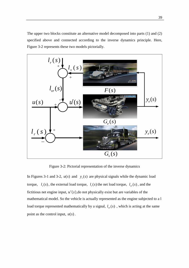
The upper two blocks constitute an alternative model decomposed into parts (1) and (2)
specified above and connected according to the inverse dynamics principle. Here,
Figure 3-2 represents these two models pictorially.
( )rl s
( )vG s
( )eG s
( )F s
( )ey s
( )ey s
( )u s ( )u s
( )vrl s
( )rl s
( )vl s
Figure 3-2: Pictorial representation of the inverse dynamics
In Figures 3-1 and 3-2, ( )u s and ( )vy s are physical signals while the dynamic load
torque, ( )vl s , the external load torque, ( )rl s the net load torque, ( )vrl s , and the
fictitious net engine input, ( ),do not physically exist but are variables of the
mathematical model. So the vehicle is actually represented as the engine subjected to a l
load torque represented mathematically by a signal, ( )vrl s , which is acting at the same
point as the control input, ( )u s .
40
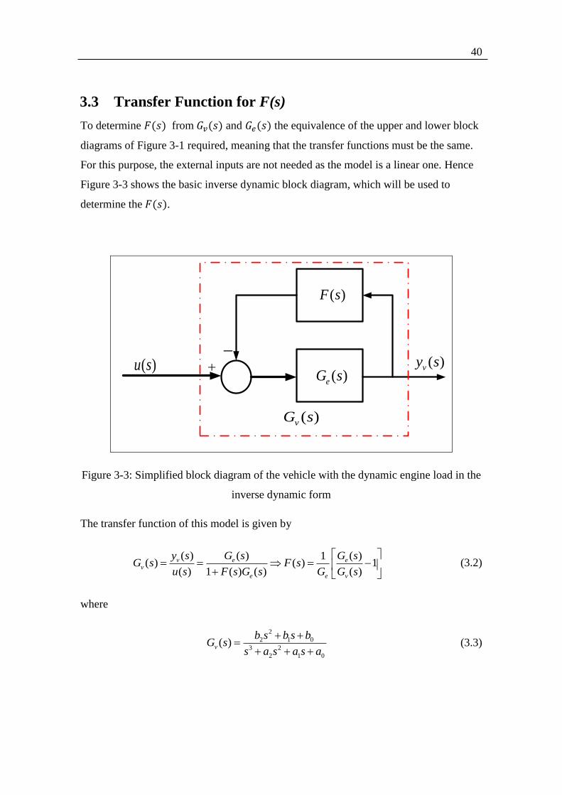
3.3 Transfer Function for F(s)
To determine ( ) from ( ) and ( ) the equivalence of the upper and lower block
diagrams of Figure 3-1 required, meaning that the transfer functions must be the same.
For this purpose, the external inputs are not needed as the model is a linear one. Hence
Figure 3-3 shows the basic inverse dynamic block diagram, which will be used to
determine the ( ).
( )eG s
( )F s
( )vy s( )u s
( )vG s
Figure 3-3: Simplified block diagram of the vehicle with the dynamic engine load in the
inverse dynamic form
The transfer function of this model is given by
( ) ( ) ( )1
( ) ( ) 1( ) 1 ( ) ( ) ( )
v e ev
e e v
y s G s G sG s F s
u s F s G s G G s
(3.2)
where
2
2 1 0
3 2
2 1 0
( )v
b s b s bG s
s a s a s a
(3.3)
41
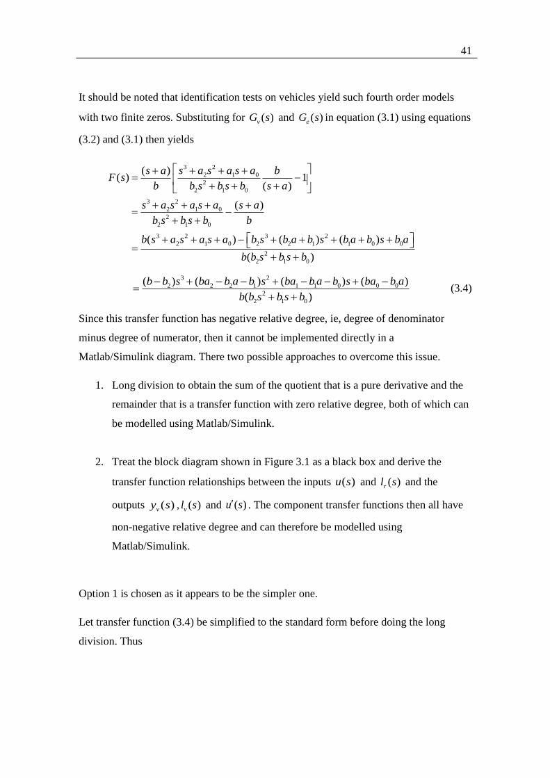
It should be noted that identification tests on vehicles yield such fourth order models
with two finite zeros. Substituting for ( )vG s and ( )eG s in equation (3.1) using equations
(3.2) and (3.1) then yields
3 2
2 1 0
2
2 1 0
3 2
2 1 0
2
2 1 0
3 2 3 2
2 1 0 2 2 1 1 0 0
2
2 1 0
( )( ) 1
( )
( )
( ) ( ) ( )
( )
s a s a s a s a bF s
b b s b s b s a
s a s a s a s a
b s b s b b
b s a s a s a b s b a b s b a b s b a
b b s b s b
3 2
2 2 2 1 1 1 0 0 0
2
2 1 0
( ) ( ) ( ) ( )
( )
b b s ba b a b s ba b a b s ba b a
b b s b s b
(3.4)
Since this transfer function has negative relative degree, ie, degree of denominator
minus degree of numerator, then it cannot be implemented directly in a
Matlab/Simulink diagram. There two possible approaches to overcome this issue.
1. Long division to obtain the sum of the quotient that is a pure derivative and the
remainder that is a transfer function with zero relative degree, both of which can
be modelled using Matlab/Simulink.
2. Treat the block diagram shown in Figure 3.1 as a black box and derive the
transfer function relationships between the inputs ( )u s and ( )rl s and the
outputs ( )vy s , ( )vl s and ( )u s . The component transfer functions then all have
non-negative relative degree and can therefore be modelled using
Matlab/Simulink.
Option 1 is chosen as it appears to be the simpler one.
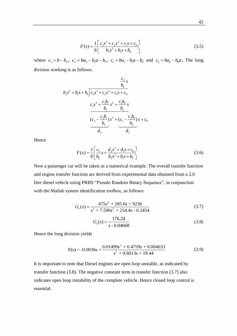
Let transfer function (3.4) be simplified to the standard form before doing the long
division. Thus
42
3 2
3 2 1 0
2
2 1 0
1( )
c s c s c s cF s
b b s b s b
(3.5)
where 3 2c b b , 2 2 2 1c ba b a b , 1 1 1 0c ba b a b and 0 0 0c ba b a . The long
division working is as follows.
3
2
2 3 2
2 1 0 3 2 1 0
3 23 1 3 03
2 2
23 1 3 02 1 0
2 2
2 1
( ) ( )
cs
b
b s b s b c s c s c s c
c b c bc s s s
b b
c b c bc s c s c
b b
d d
Hence
2
3 2 1 0
2
2 2 1 0
1( )
c d s d s cF s s
b b b s b s b
(3.6)
Now a passenger car will be taken as a numerical example. The overall transfer function
and engine transfer function are derived from experimental data obtained from a 2.0
litre diesel vehicle using PRBS “Pseudo Random Binary Sequence”, in conjunction
with the Matlab system identification toolbox, as follows:
2
3 2
475s + 285.6s + 9236( )
s + 7.596s + 254.4s - 0.2454vG s (3.7)
176.24
( )s - 0.04668
eG s (3.8)
Hence the long division yields
2
2
0.01499s + 0.4759s + 0.004633F(s) = -0.0036s +
s + 0.6013s + 19.44 (3.9)
It is important to note that Diesel engines are open loop unstable, as indicated by
transfer function (3.8). The negative constant term in transfer function (3.7) also
indicates open loop instability of the complete vehicle. Hence closed loop control is
essential.

43
3.4 The Concept of Observer Based Load Estimation
Figure 3-4 represents a first order plant with control input, ( )u s , disturbance input,
( )d s , and output, ( )y s together with a model with the same input, additional input,
( )l s , and output, ˆ( )y s .
( )d s
( )l s
1
s a
1
ˆs a
( )y s
ˆ( )y s
( )u s
Plant
Model
Figure 3-4: A first order plant and its model
It will now be shown that there exists an additional input, ( )l s , that yields ˆ( ) ( )y s y s .
This is not only the basis of the observer based load estimation but also that of the
OBRC of Chapter 4. The transfer function relationships of Figure 3-4 are as follows:
1
( ) ( ) ( )y s u s d ss a
(3.10)
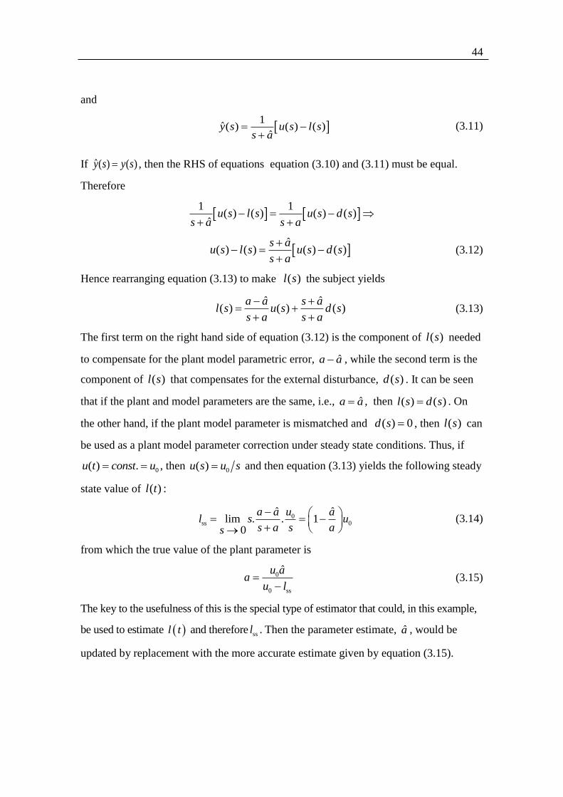
44
and
1
ˆ( ) ( ) ( )ˆ
y s u s l ss a
(3.11)
If ˆ( ) ( )y s y s , then the RHS of equations equation (3.10) and (3.11) must be equal.
Therefore
1 1
( ) ( ) ( ) ( )ˆ
u s l s u s d ss a s a
ˆ
( ) ( ) ( ) ( )s a
u s l s u s d ss a
(3.12)
Hence rearranging equation (3.13) to make ( )l s the subject yields
ˆ ˆ
( ) ( ) ( )a a s a
l s u s d ss a s a
(3.13)
The first term on the right hand side of equation (3.12) is the component of ( )l s needed
to compensate for the plant model parametric error, ˆa a , while the second term is the
component of ( )l s that compensates for the external disturbance, ( )d s . It can be seen
that if the plant and model parameters are the same, i.e., ˆa a , then ( ) ( )l s d s . On
the other hand, if the plant model parameter is mismatched and ( ) 0d s , then ( )l s can
be used as a plant model parameter correction under steady state conditions. Thus, if
0( ) .u t const u , then 0( )u s u s and then equation (3.13) yields the following steady
state value of ( ) :l t
0ss 0
ˆ ˆlim . . 1
0
a a u al s u
s a s as
(3.14)
from which the true value of the plant parameter is
0
0 ss
ˆu aa
u l
(3.15)
The key to the usefulness of this is the special type of estimator that could, in this example,
be used to estimate l t and therefore ssl . Then the parameter estimate, a , would be
updated by replacement with the more accurate estimate given by equation (3.15).

45
Figure 3-5 shows the overall structure of the system providing an estimate, vrˆ ( )l s , of
the net engine load torque, vr ( )l s , shown in Figure 3-1.
Load
Estimator
(observer)
( )u s
( )vrl s
ˆ ( )vrl s
( )vy s
ˆ ( )vy s
Physical Engine
176.24
0.04668s
( )ve s
Model Correction
Loop
Figure 3-5: Block diagram of the external load estimator
Essentially, the load estimator contains a model of the engine driven by the same input,
( )u s , as applied to the physical engine. This generates an estimate, ˆ ( )vy s of the
measured engine speed, ( )vy s , together with the required engine load torque estimate,
vrˆ ( )l s . An error, v
ˆ( ) ( ) ( )v ve s y s y s , is formed and fed back to the engine model to
correct its output so that v ( ) 0e t . If the engine model is accurate, then once v ( ) 0e t ,
vrˆ ( )l t is a good estimate of vr ( )l t .
The following section presents the observer and the steps of its design.
3.5 The Observer and its Design
46
1k
s
1
s
0k
a
( )u s b
( )vy s
ˆ ( )vy s
ˆ ( )vrl s( )ve s
Engine
Model
Model Correction
Loop
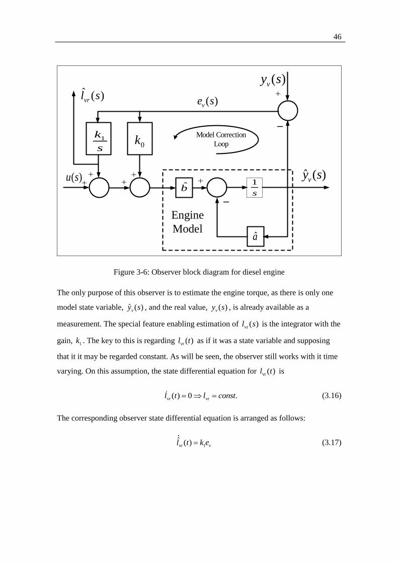
Figure 3-6: Observer block diagram for diesel engine
The only purpose of this observer is to estimate the engine torque, as there is only one
model state variable, ˆ ( )vy s , and the real value, ( )vy s , is already available as a
measurement. The special feature enabling estimation of vr ( )l s is the integrator with the
gain, 1k . The key to this is regarding vr ( )l t as if it was a state variable and supposing
that it it may be regarded constant. As will be seen, the observer still works with it time
varying. On this assumption, the state differential equation for vr ( )l t is
vr vr( ) 0 .l t l const (3.16)
The corresponding observer state differential equation is arranged as follows:
vr 1ˆ ( ) vl t k e (3.17)
47
where 1k is a constant gain. This enables
ve to continually correct vrl until the correction
loop drives ve to approximately zero, whereupon
vrl will have converged almost to the
correct value. From equation (3.17),
1vr 1 vr
0
ˆ ˆ( ) ( ) ( ) ( )t
v v
kl t k e d l s e s
s (3.18)
The observer block diagram agrees with this.
To calculate the observer gains, 0k and
1k , in the block diagram of Figure 3.6, the
method of pole assignment is used. the first the characteristic equation of the observer is
needed in terms of these gains. This is obtained in straightforward fashion by equating
the determinant of Mason’s Rule to zero. The signal flow graph is not needed as the
block diagram contains the same information Hence
210 0 1
ˆ1 ˆ ˆ ˆˆ ˆ1 0 0bk
a bk s a bk s bks s
(3.19)
It should be noted, however, that in cases of higher order, particularly those having a
complex loop structure, it will be more economical in time and effort to use the
numerical method of Appendix A2.
The Dodds 5% settling time formula (2.11will now be used for the pole placement
design to achieve a correction loop settling time of soT . Thus
1.5(1 )so coT n T (3.20)
By inspection of Figure 3.6 the order of the observer is 2n and the two poles are
placed at
1,2 2
1 1.5(1 ) 9
2n
co so so
ns
T T T
(3.21)
Hence, the desired characteristic polynomial is given by
2 2
2
9 9 81( )
2 2 4so so so
s s sT T T
(3.22)

48
This must be the same as the characteristic polynomial of equation (3.19). Thus
2 2
0 1 2
9 81ˆ ˆˆ( )2 4so so
s a bk s bk s sT T
Equating the coefficients of like powers of s then yields the following formulae for the
observer gains:
0 1 2
1 9 81ˆ and
ˆ ˆ4so so
k a kTb T b
(3.23)
The observer variable, ˆ ( )vy t , will track the measured signal, ( )vy t and vrl t will track
the time varying engine load torque, vrl t more closely if the observer settling time is
made smaller. Typically the 5so sT T , where sT is the settling time of the control
system of which the observer is part. Transients occur due to load changes, which may
come from the driving conditions or gear changes. Hence, the value for soT is chosen to
be considerably smaller than the typical settling time of the engine speed. The vehicle is
much more responsive to the driver demand when the vehicle is unloaded than when it
is fully loaded. A typical 10litre engine will accelerate from low idle (500 rpm) to high
idle (2000 rpm) in approximately 1.5 sec. Hence a value of 0.01secsoT was chosen,
yielding 1 1149k and 0 5.109k .
3.6 Passenger Car Inverse Dynamic Simulation
3.6.1 Overview
In this section, the simulation results of the inverse dynamic model of the vehicle are
validated by comparison with those of the standard form of the vehicle model, which
should be the same. The load torque observer is included in both simulations to check
its performance. The simulation is performed in two modes: open and closed loop.
49
3.6.2 Observer Simulation Results
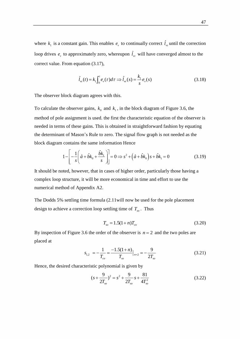
In the open loop mode, both plant models and the observer are driven by a piecewise
constant common control torque, ( )u t , as shown in Figure 3-5
( )eG s
( )F s
u
Observer
rl
rl
rvl
( )vG s
ˆrvl
ˆvy
[sec]Time
Torque[Nm]
Inverse Dynamic Model of Vehicle
Standard Model of Vehicle
vinvy
v stdy
Figure 3-5 Open loop block diagram of inverse dynamics and vehicle model with observer
50
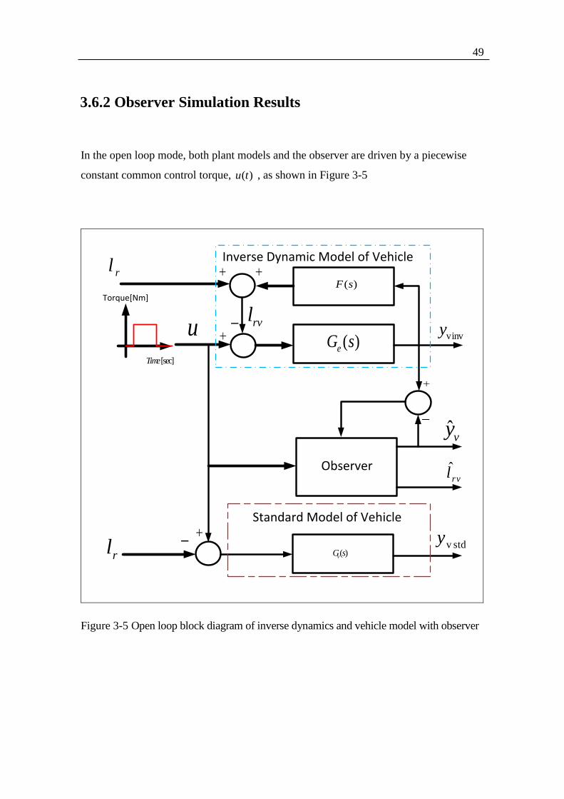
The open loop input, ( )u t , is a step from zero to a constant positive value at 1[ ]t s
followed by another step returning to zero at 8[ ]t s .
Figure 3.6 shows the plot of ( )vy t , ˆ ( )vy t and the observer error,
m vinv vstd( ) ( ) ( )ve t y t y t .
0 1 2 3 4 5 6 7 8 9 100
200
400
Engi
neS
pee
d [
rpm
]
Time [sec]
Open loop of Ge(s) and Gv(s)
0 1 2 3 4 5 6 7 8 9 10-10
0
10
Erro
r [r
pm
]
invy
stdy
( )std invy y
Figure 3-6 Open loop speed response of inverse dynamic and standard models
The oscillation at the start and end of the step is due to the complex conjugate poles of
( )vG s . The error ( ) yv std inve t y is small as shown Figure 3.6.
Figure 3.7 shows the ability of the observer to estimate the external load torque.
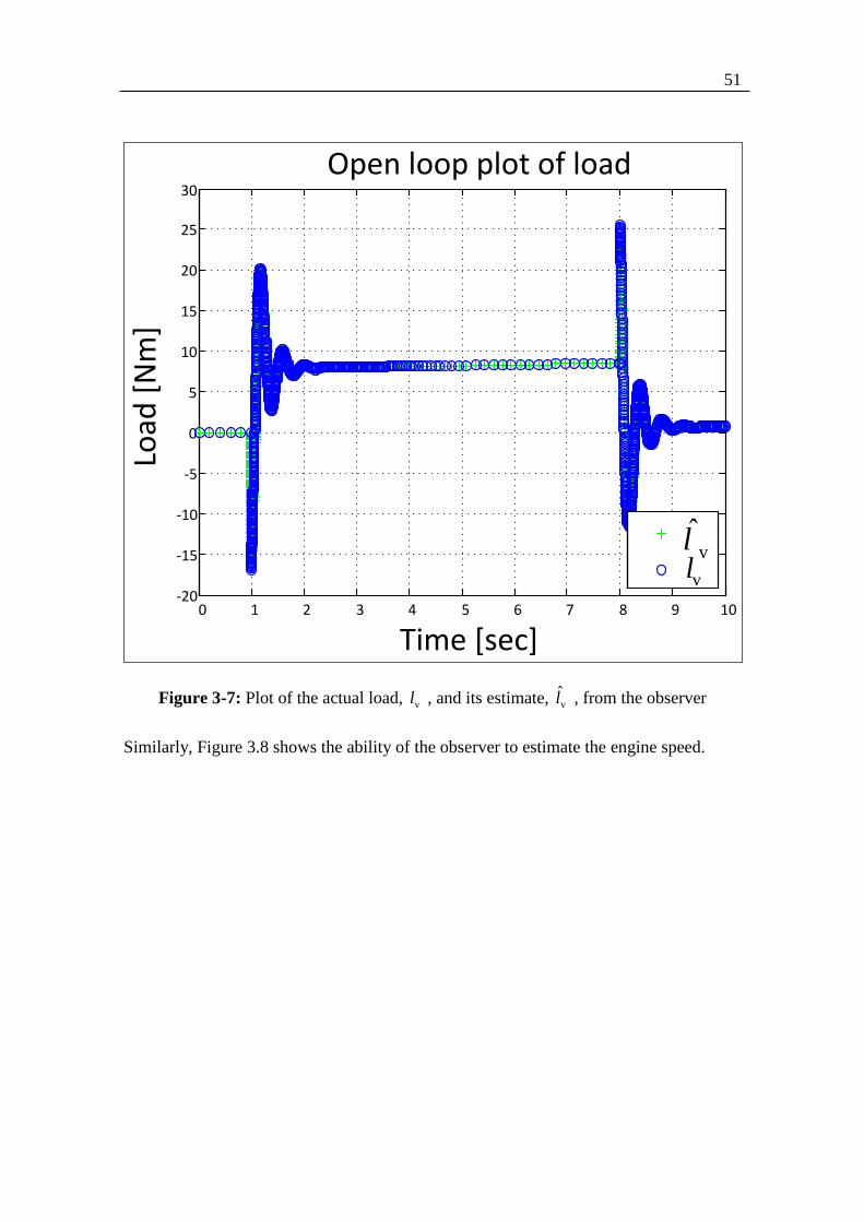
51
0 1 2 3 4 5 6 7 8 9 10-20
-15
-10
-5
0
5
10
15
20
25
30
Load
[N
m]
Time [sec]
Open loop plot of load
vlvl
Figure 3-7: Plot of the actual load, vl , and its estimate, vl , from the observer
Similarly, Figure 3.8 shows the ability of the observer to estimate the engine speed.

52
0 1 2 3 4 5 6 7 8 9 100
200
400
Engi
ne
Spee
d[r
pm
]Open loop plot of Engine Speed and Torque
Time [sec]
0 1 2 3 4 5 6 7 8 9 100
2.4
4.8
7.2
9.6
12
Torq
ue
[rp
m]
invy
stdy
Applied Torque
Figure 3-8 Engine speed, vy , estimated engine speed, vy and external load torque
Next the simulation results in the closed loop mode are presented. Here, ( )u t is
produced by a simple proportional speed controller acting on the output of the inverse
dynamic model, while the same input is applied to the standard model. The purpose of
this simulation is to confirm that the two models are still equivalent under closed loop
control and the observer continues to work correctly.
53
( )eG s
( )F s
u
Observer
rl
rl
rvl
( )vG s
rypk
Standard Model of Vehicle
Inverse Dynamic Model of Vehicle
ˆrvl
ˆvy
vinvy
v stdy
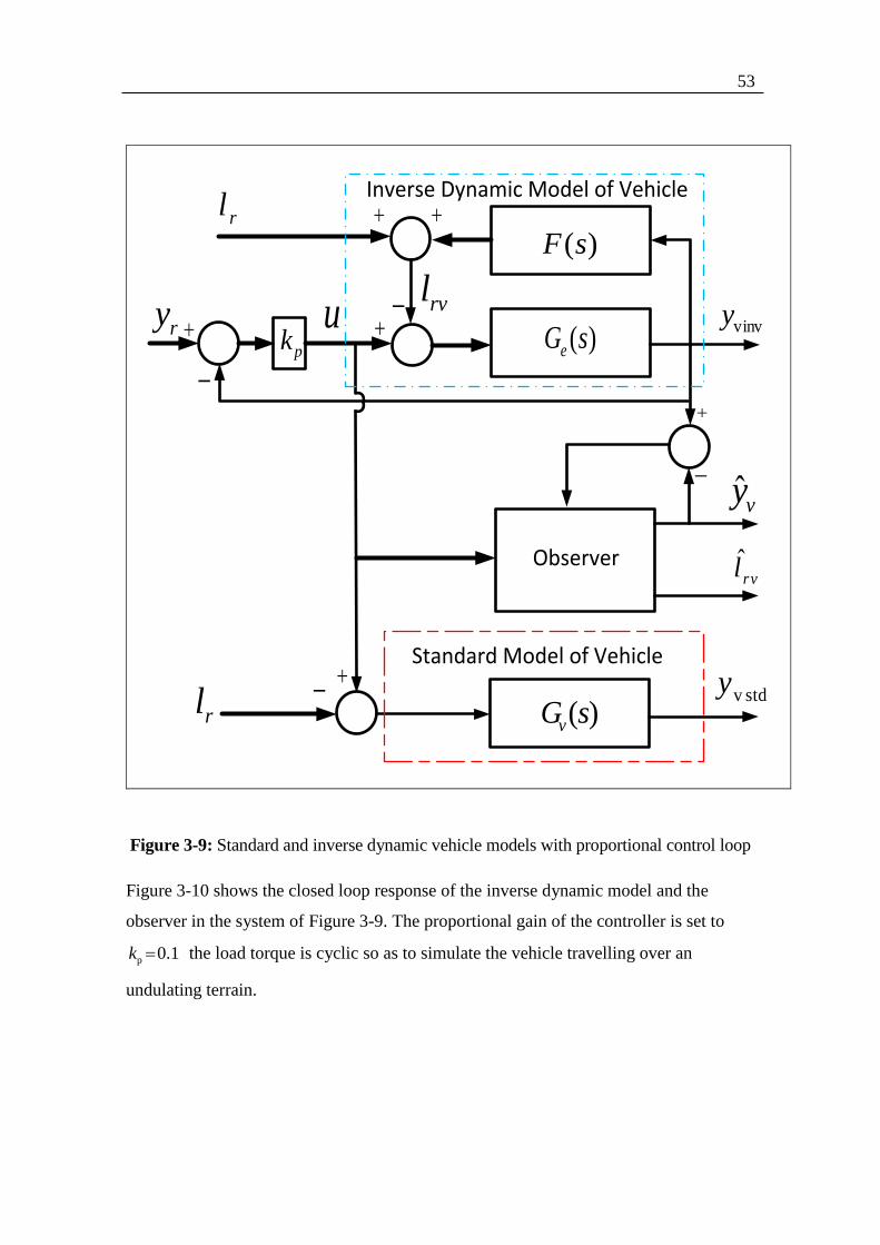
Figure 3-9: Standard and inverse dynamic vehicle models with proportional control loop
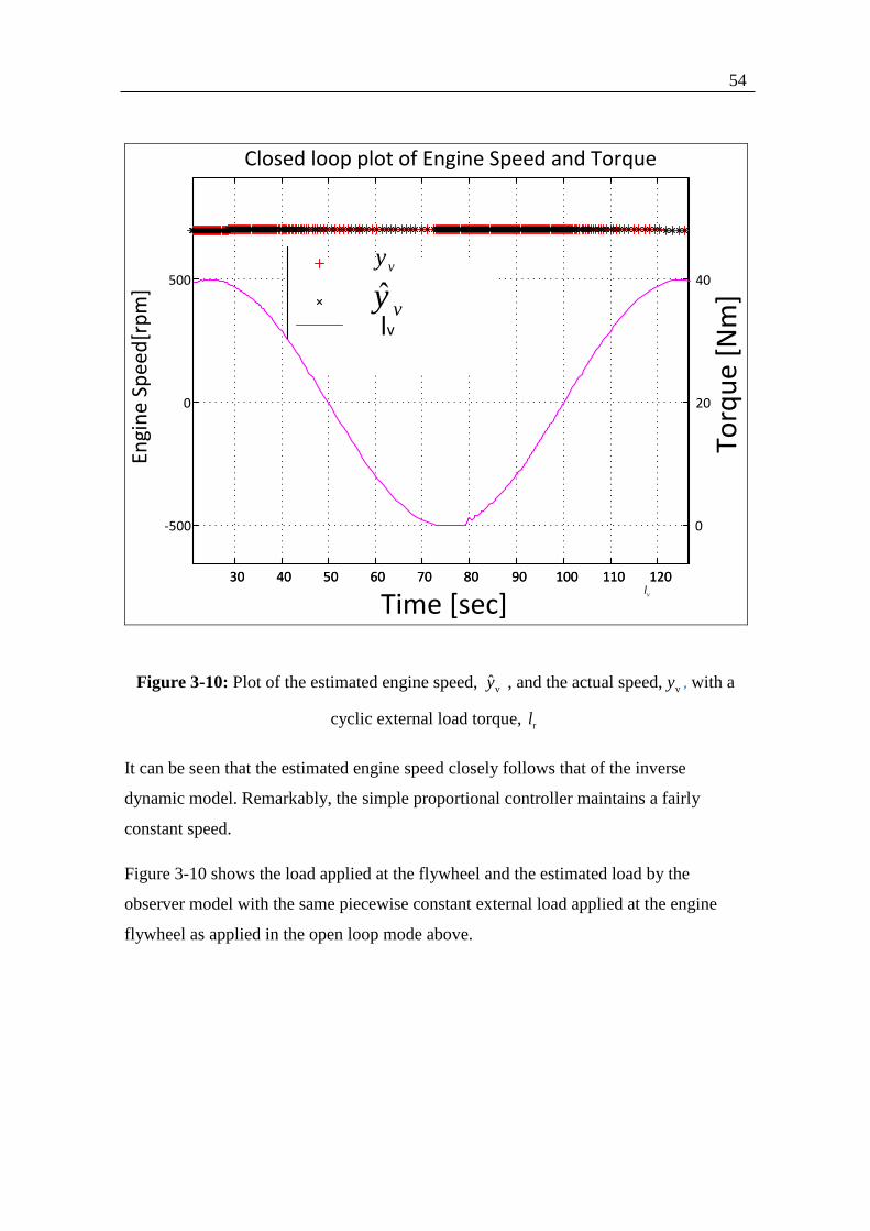
Figure 3-10 shows the closed loop response of the inverse dynamic model and the
observer in the system of Figure 3-9. The proportional gain of the controller is set to
p 0.1k the load torque is cyclic so as to simulate the vehicle travelling over an
undulating terrain.
54
30 40 50 60 70 80 90 100 110 120
-500
0
500
Engi
ne
Spee
d[r
pm
]Closed loop plot of Engine Speed and Torque
Time [sec]
30 40 50 60 70 80 90 100 110 120
0
20
40
Torq
ue
[Nm
]
lv
ˆvy
vy
vl
Figure 3-10: Plot of the estimated engine speed, vy , and the actual speed, vy , with a
cyclic external load torque, rl
It can be seen that the estimated engine speed closely follows that of the inverse
dynamic model. Remarkably, the simple proportional controller maintains a fairly
constant speed.
Figure 3-10 shows the load applied at the flywheel and the estimated load by the
observer model with the same piecewise constant external load applied at the engine
flywheel as applied in the open loop mode above.

55
0 1 2 3 4 5 6 7 8 9 10-20
-15
-10
-5
0
5
10
15
20
25
30
Load
[N
m]
Time [sec]
Closed loop plot of Load
lr
lrv
ˆrvl
Figure 3-11: plot of the estimated load and inverse dynamic load
It can be seen that the estimation of this load is very good and is within an acceptable
margin of error. During the transient condition, the observer estimation will be lagging
the actual load. However, this transient estimation error is too small to be discernible in
Figure 3-11 and is acceptable
56
3.6.3 Formulation of the unloaded Engine Model
An engine is a highly nonlinear system but can be approximated as a linear system with
a very narrow band of linearity around the operating point. A simple physical model of
the engine is used as a plant model. This is a torque proportional to the fuel flow rate, u
, via a constant, eK , called the engine gain, applied to a balanced body with moment of
inertia, eJ , subject to a friction torque, r , that is proportional to the crankshaft angular
velocity, , via a constant, B , that is a function of the oil and coolant temperature, o .
The torque balance equation of this model is as follows:
e e oJ K u B (3.24)
For a given engine speed, the friction force will increase when the engine is cold and
decrease as the engine warms up (cold to hot). The oil and coolant temperature of the
engine, however, will have a DC effect on the frictional force in the sense that it will be
sufficiently slowly varying to be considered constant on the time scale of operation of
the control system. Then oB may be replaced by simply B in the equations of the
model. The injection timing affects eK but since this will be considered fixed during the
control system operation, eK is a constant plant parameter.. Figure 3.12 shows the
engine block diagram based on the following re-arrangement of equation (3.24):
1
e
e
K u BJ
Taking Laplace transforms with zero initial conditions then yields
1 1
( ) ( ) ( ) ( ) ( ) ( )e e
e e
s s K u s B s s K u s B sJ J s
Figure 3-11 directly corresponds to this transfer function relationship.
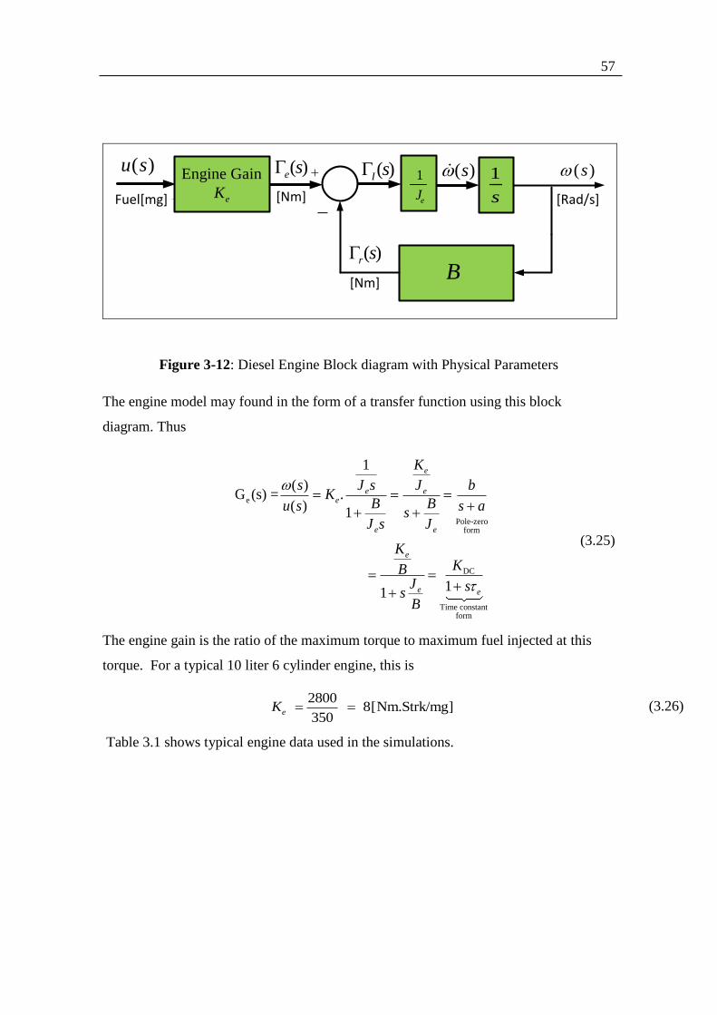
57
[Nm]
Fuel[mg] [Nm]
1
s
1
eJ
Engine Gain
eK
( )u s ( )e s
( )r sB
( )I s ( )s( )s
[Rad/s]
Figure 3-12: Diesel Engine Block diagram with Physical Parameters
The engine model may found in the form of a transfer function using this block
diagram. Thus
e
Pole-zeroform
DC
Time constantform
1
( )G (s) = .
( ) 1
11
e
e ee
e e
e
e e
K
s bJ s JK
B Bu s s asJ s J
KKB
J ssB
(3.25)
The engine gain is the ratio of the maximum torque to maximum fuel injected at this
torque. For a typical 10 liter 6 cylinder engine, this is
2800
8[Nm.Strk/mg]350
eK (3.26)
Table 3.1 shows typical engine data used in the simulations.
58
Table 3.1: Typical data for a 10 L 6 cylinder Diesel engine
Name Values Units
Capacity 10 L
Total moment of inertia, eJ 4.0 2kgm
Friction torque at 500[rpm] 120 Nm
Friction coefficient, B 2.29 Nm/(rad/s)
Maximum torque 2800 Nm
Maximum fuel injection per
stroke
350 Mg/stroke
Then the constant parameters of equation (3.25) are as follows.
28 2 [strk/mg s ]
4.0
e
e
Kb
J
12.29
0.57 s4e
Ba
J
2
DC
8 3.49 [Nm.Strk/mg/s ]
2.29
eKK
B
and
4
0.03 [s]120
ee
J
B
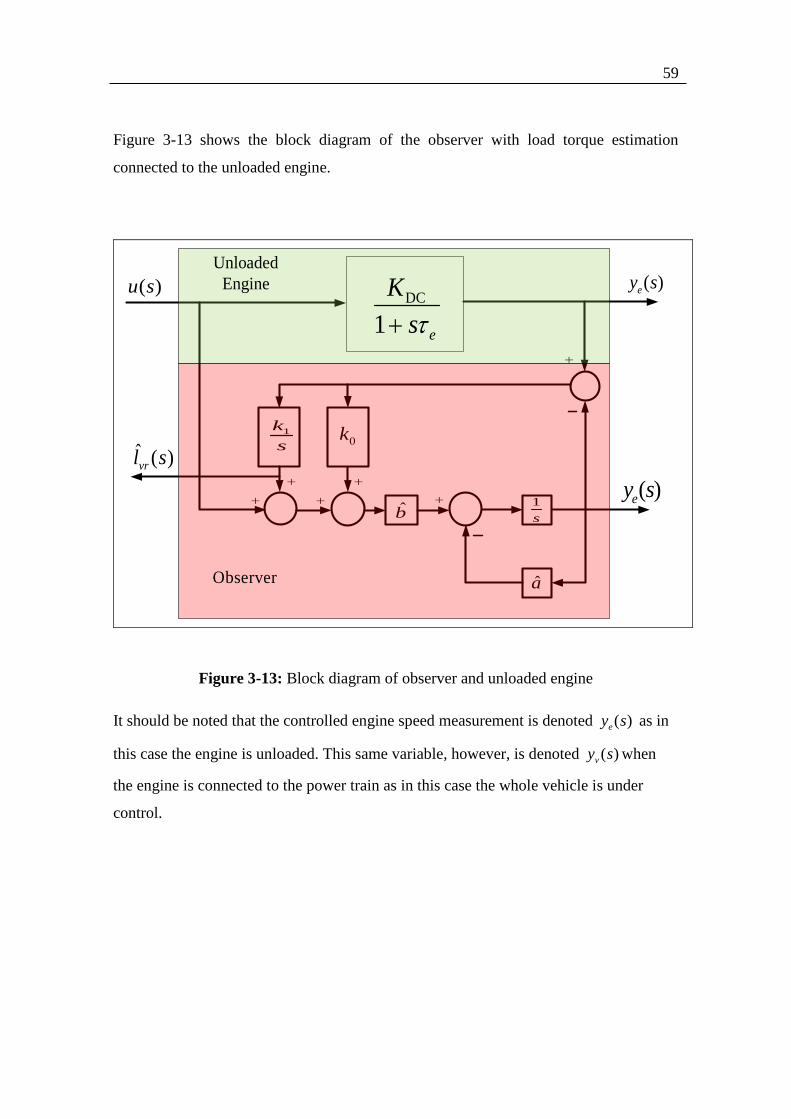
59
Figure 3-13 shows the block diagram of the observer with load torque estimation
connected to the unloaded engine.
( )ey s
1k
s
1
s
0k
a
( )u s
b
DC
1 e
K
s
( )ey s
ˆ ( )vrl s
Observer
Unloaded
Engine
Figure 3-13: Block diagram of observer and unloaded engine
It should be noted that the controlled engine speed measurement is denoted ( )ey s as in
this case the engine is unloaded. This same variable, however, is denoted ( )vy s when
the engine is connected to the power train as in this case the whole vehicle is under
control.
60
4 Observer Based Robust Control (OBRC): General Theory
4.1 Overview
Observer based robust control (OBRC) is a relatively new method [33]. This is based on
an observer designed to estimate the equivalent disturbance input referred to the control
input to a plant. The key to the method is that it represents plant modeling errors as well
as external disturbances. This equivalent disturbance estimate is applied to the real plant
input and the model of the plant in the observer to cancel its effect, thereby reducing the
control problem to that of controlling the known real-time model of the plant employed
in the observer. One of the disadvantages of conventional robust control methods such
as those based on sliding mode control is that relatively high gain control loops are
closed around the uncertain plant, thereby risking instability. The original motivation
for considering OBRC is the fact that the high gain loops in the system were apparently
restricted to the observer. Thus, applying it to a known plant model avoids any risk of
instability. As will be seen, a step in the formation of an OBRC controller will convert
the problem of controlling an uncertain plant to the simple one of controlling the known
model in the observer. This step, however, also effectively transfers the high gain loops
of the observer to the unknown plant. Despite this, OBRC is included in view of its
unconventional structure. Due to this, different results may be expected than those from
other control techniques, such as robust pole placement, which directly close high gain
loops around the uncertain plant. The method is demonstrated via its application to
Diesel Drivelines for commercial road vehicles.
One of the operational problems with conventional PI engine speed controllers is the
need for time consuming initial controller tuning, requiring different sets of gains for
each gear selection, including idle (i.e., neutral) and later retuning to compensate for
changes in the driveline characteristics with component ageing. A major advantage of
OBRC in this application is the elimination of the tuning procedure. Also, of particular
interest is the fact that the order of the system is increased by two when a gearbox is
considered in the transfer function of the system.
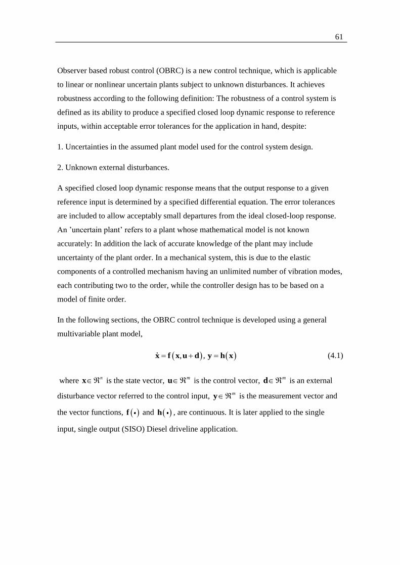
61
Observer based robust control (OBRC) is a new control technique, which is applicable
to linear or nonlinear uncertain plants subject to unknown disturbances. It achieves
robustness according to the following definition: The robustness of a control system is
defined as its ability to produce a specified closed loop dynamic response to reference
inputs, within acceptable error tolerances for the application in hand, despite:
1. Uncertainties in the assumed plant model used for the control system design.
2. Unknown external disturbances.
A specified closed loop dynamic response means that the output response to a given
reference input is determined by a specified differential equation. The error tolerances
are included to allow acceptably small departures from the ideal closed-loop response.
An ’uncertain plant’ refers to a plant whose mathematical model is not known
accurately: In addition the lack of accurate knowledge of the plant may include
uncertainty of the plant order. In a mechanical system, this is due to the elastic
components of a controlled mechanism having an unlimited number of vibration modes,
each contributing two to the order, while the controller design has to be based on a
model of finite order.
In the following sections, the OBRC control technique is developed using a general
multivariable plant model,
, , x f x u d y h x (4.1)
where nx is the state vector,
mu is the control vector, md is an external
disturbance vector referred to the control input, my is the measurement vector and
the vector functions, f and h , are continuous. It is later applied to the single
input, single output (SISO) Diesel driveline application.
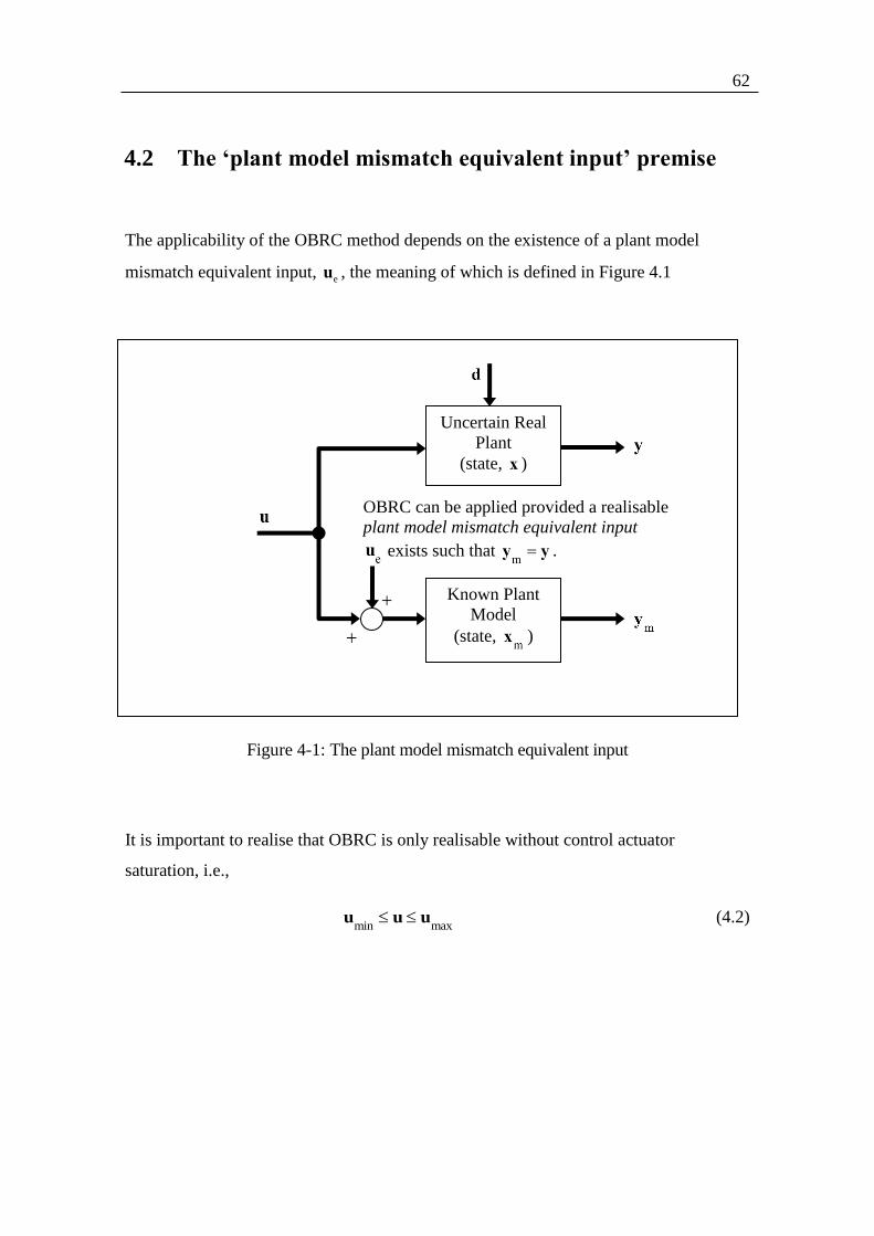
62
4.2 The ‘plant model mismatch equivalent input’ premise
The applicability of the OBRC method depends on the existence of a plant model
mismatch equivalent input, eu , the meaning of which is defined in Figure 4.1
Figure 4-1: The plant model mismatch equivalent input
It is important to realise that OBRC is only realisable without control actuator
saturation, i.e.,
min max
u u u (4.2)
Uncertain Real
Plant
(state, )
Known Plant
Model
(state, )
OBRC can be applied provided a realisable
plant model mismatch equivalent input
exists such that .
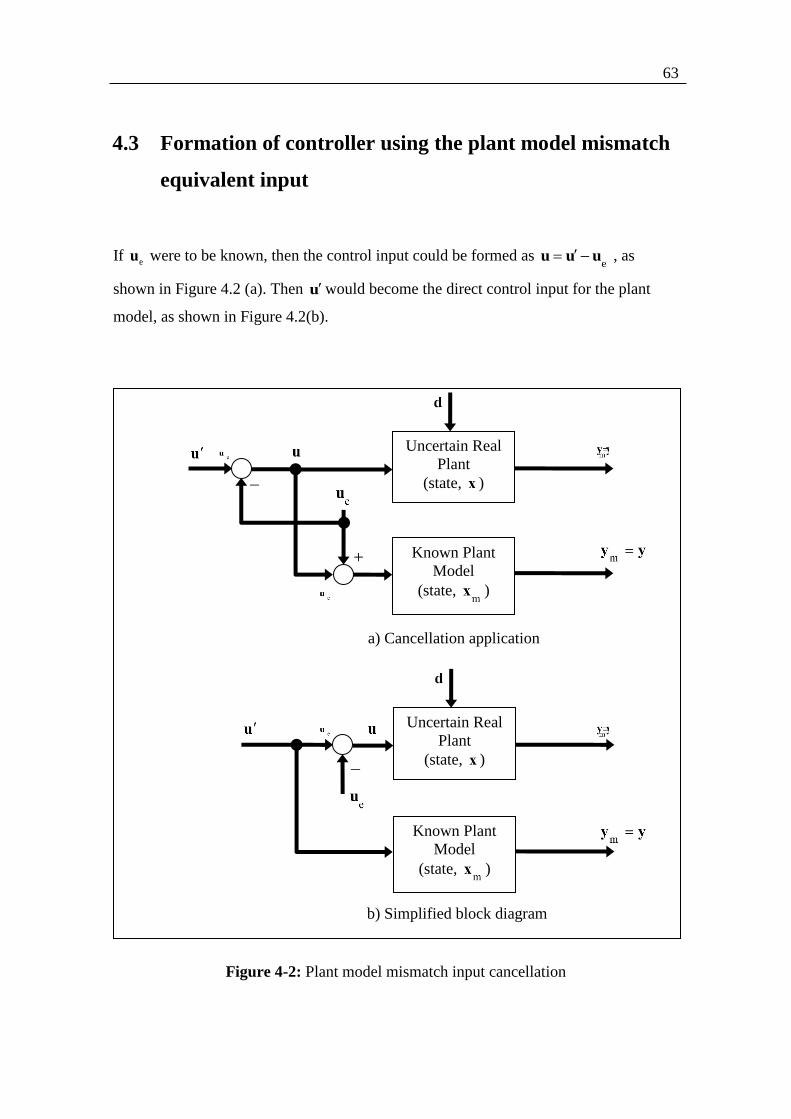
63
4.3 Formation of controller using the plant model mismatch
equivalent input
If eu were to be known, then the control input could be formed as e
u u u , as
shown in Figure 4.2 (a). Then u would become the direct control input for the plant
model, as shown in Figure 4.2(b).
Figure 4-2: Plant model mismatch input cancellation
Uncertain Real
Plant
(state, )
Known Plant
Model
(state, )
Uncertain Real
Plant
(state, )
Known Plant
Model
(state, )
a) Cancellation application
b) Simplified block diagram

64
A state feedback controller could be designed for the known plant model which would
control the real plant as my y as shown in Figure 4.3.
Figure 4-3: Controlling the uncertain real plant via control of the plant model
What is needed to render this method practicable is an estimate of eu and this is
provided by an observer as shown in the following section.
4.4 Introduction of an Observer for the Estimation of
External Disturbance
In Figure 4.3, a loop is closed around the known real time plant model, the purpose of
which is to drive the error between my and y to negligible proportions. Note that for
the formulation of an observer required to estimatee
u , it is necessary to revert to Figure
4-2 (a), since the plant control input, u , has to be applied to the known plant model. A
variant of the observer, however, will be presented subsequently that permits the
simplification depicted in Figure 4-2 (b) to be carried out again.
Uncertain Real
Plant
(state, )
Known Plant
Model
(state, )
State
Feedback
Control Law
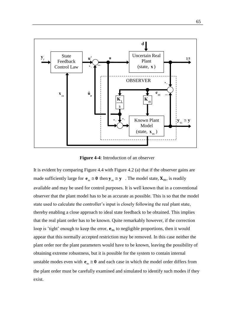
65
Figure 4-4: Introduction of an observer
It is evident by comparing Figure 4.4 with Figure 4.2 (a) that if the observer gains are
made sufficiently large for m e 0 then m y y . The model state, , is readily
available and may be used for control purposes. It is well known that in a conventional
observer that the plant model has to be as accurate as possible. This is so that the model
state used to calculate the controller’s input is closely following the real plant state,
thereby enabling a close approach to ideal state feedback to be obtained. This implies
that the real plant order has to be known. Quite remarkably however, if the correction
loop is ’tight’ enough to keep the error, to negligible proportions, then it would
appear that this normally accepted restriction may be removed. In this case neither the
plant order nor the plant parameters would have to be known, leaving the possibility of
obtaining extreme robustness, but it is possible for the system to contain internal
unstable modes even with m e 0 and each case in which the model order differs from
the plant order must be carefully examined and simulated to identify such modes if they
exist.
Uncertain Real
Plant
(state, )
Known Plant
Model
(state, )
State
Feedback
Control Law
OBSERVER
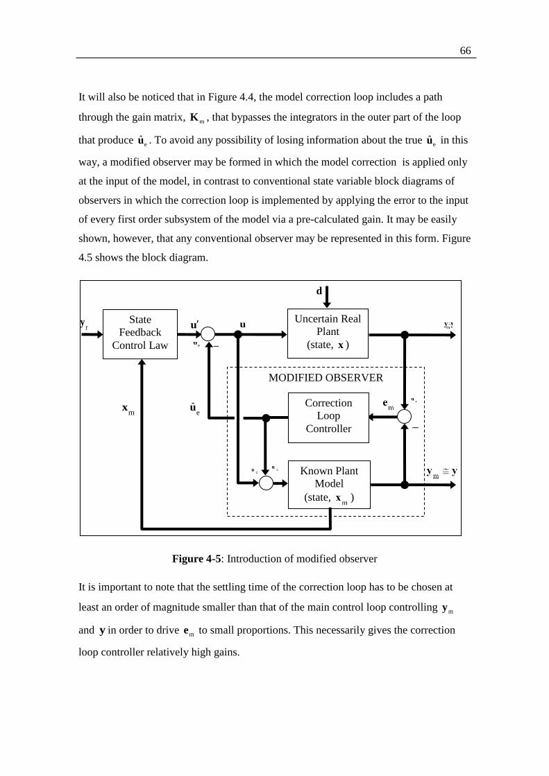
66
It will also be noticed that in Figure 4.4, the model correction loop includes a path
through the gain matrix, mK , that bypasses the integrators in the outer part of the loop
that produce eu . To avoid any possibility of losing information about the true
eu in this
way, a modified observer may be formed in which the model correction is applied only
at the input of the model, in contrast to conventional state variable block diagrams of
observers in which the correction loop is implemented by applying the error to the input
of every first order subsystem of the model via a pre-calculated gain. It may be easily
shown, however, that any conventional observer may be represented in this form. Figure
4.5 shows the block diagram.
Figure 4-5: Introduction of modified observer
It is important to note that the settling time of the correction loop has to be chosen at
least an order of magnitude smaller than that of the main control loop controlling my
and y in order to drive me to small proportions. This necessarily gives the correction
loop controller relatively high gains.
Correction
Loop
Controller
Known Plant
Model
(state, )
MODIFIED OBSERVER
Uncertain Real
Plant
(state, x )
d
u
eu
eu
u State
Feedback
Control Law
mx
ry
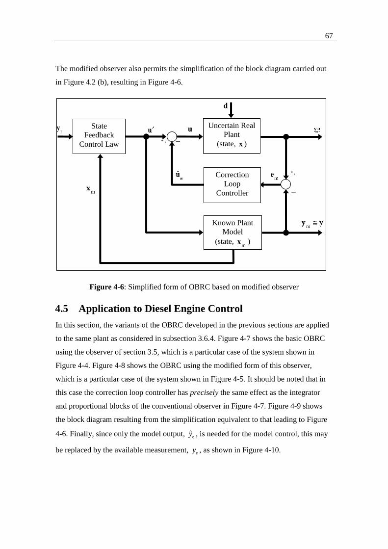
67
The modified observer also permits the simplification of the block diagram carried out
in Figure 4.2 (b), resulting in Figure 4-6.
Figure 4-6: Simplified form of OBRC based on modified observer
4.5 Application to Diesel Engine Control
In this section, the variants of the OBRC developed in the previous sections are applied
to the same plant as considered in subsection 3.6.4. Figure 4-7 shows the basic OBRC
using the observer of section 3.5, which is a particular case of the system shown in
Figure 4-4. Figure 4-8 shows the OBRC using the modified form of this observer,
which is a particular case of the system shown in Figure 4-5. It should be noted that in
this case the correction loop controller has precisely the same effect as the integrator
and proportional blocks of the conventional observer in Figure 4-7. Figure 4-9 shows
the block diagram resulting from the simplification equivalent to that leading to Figure
4-6. Finally, since only the model output, ey , is needed for the model control, this may
be replaced by the available measurement, ey , as shown in Figure 4-10.
Correction
Loop
Controller
Known Plant
Model
(state, )
Uncertain Real
Plant
(state, x )
d
State
Feedback
Control Law
mx
ry
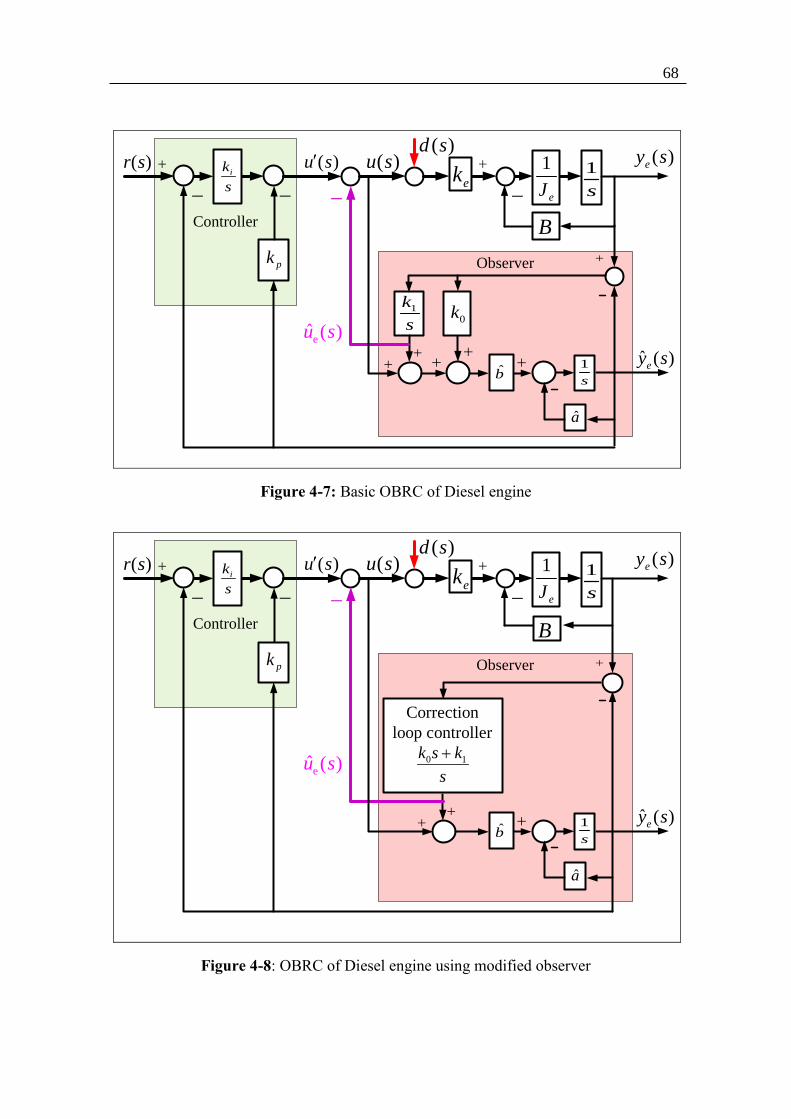
68
Controller
Observer
ik
s
1k
s
1
s
0k
a
b
1
s
pk
( )r sek
1
eJ
( )ey s
ˆ ( )ey s
B
( )u s( )u s
eˆ ( )u s
( )d s
Figure 4-7: Basic OBRC of Diesel engine
Controller
Observer
ik
s
1
s
a
b
1
s
pk
( )r sek
1
eJ
( )ey s
ˆ ( )ey s
B
( )u s( )u s
eˆ ( )u s
( )d s
0 1
Correction
loop controller
k s k
s
Figure 4-8: OBRC of Diesel engine using modified observer

69
Controller
ik
s
1
s
a
b
1
s
pk
( )r sek
1
eJ
( )ey s
ˆ ( )ey s
B
( )u s( )u s
eˆ ( )u s
( )d s
0 1
Correction
loop controller
k s k
s
Plant Model
Figure 4-9: Simplified OBRC of Diesel Engine
Controller
Observer
ik
s
1k
s
1
s
0k
a
b
1
s
pk
( )r sek
1
eJ
( )ey s
ˆ ( )ey s
B
( )u s( )u s
eˆ ( )u s
( )d s
Figure 4-10: Basic OBRC of Diesel engine with direct plant control
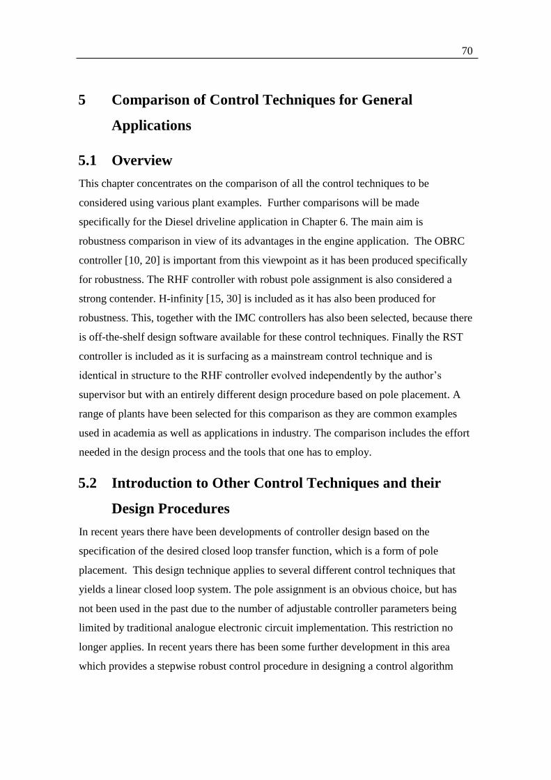
70
5 Comparison of Control Techniques for General
Applications
5.1 Overview
This chapter concentrates on the comparison of all the control techniques to be
considered using various plant examples. Further comparisons will be made
specifically for the Diesel driveline application in Chapter 6. The main aim is
robustness comparison in view of its advantages in the engine application. The OBRC
controller [10, 20] is important from this viewpoint as it has been produced specifically
for robustness. The RHF controller with robust pole assignment is also considered a
strong contender. H-infinity [15, 30] is included as it has also been produced for
robustness. This, together with the IMC controllers has also been selected, because there
is off-the-shelf design software available for these control techniques. Finally the RST
controller is included as it is surfacing as a mainstream control technique and is
identical in structure to the RHF controller evolved independently by the author’s
supervisor but with an entirely different design procedure based on pole placement. A
range of plants have been selected for this comparison as they are common examples
used in academia as well as applications in industry. The comparison includes the effort
needed in the design process and the tools that one has to employ.
5.2 Introduction to Other Control Techniques and their
Design Procedures
In recent years there have been developments of controller design based on the
specification of the desired closed loop transfer function, which is a form of pole
placement. This design technique applies to several different control techniques that
yields a linear closed loop system. The pole assignment is an obvious choice, but has
not been used in the past due to the number of adjustable controller parameters being
limited by traditional analogue electronic circuit implementation. This restriction no
longer applies. In recent years there has been some further development in this area
which provides a stepwise robust control procedure in designing a control algorithm
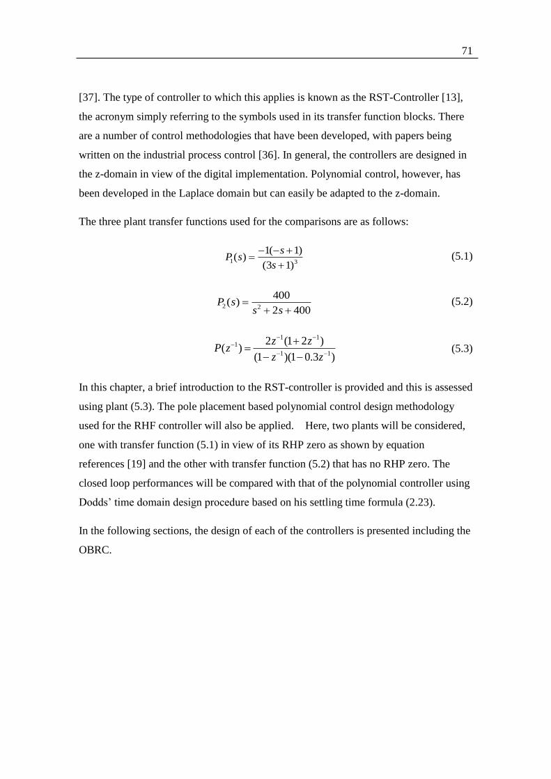
71
[37]. The type of controller to which this applies is known as the RST-Controller [13],
the acronym simply referring to the symbols used in its transfer function blocks. There
are a number of control methodologies that have been developed, with papers being
written on the industrial process control [36]. In general, the controllers are designed in
the z-domain in view of the digital implementation. Polynomial control, however, has
been developed in the Laplace domain but can easily be adapted to the z-domain.
The three plant transfer functions used for the comparisons are as follows:
1 3
1( 1)( )
(3 1)
sP s
s
(5.1)
2 2
400( )
2 400P s
s s
(5.2)
1 11
1 1
2 (1 2 )( )
(1 )(1 0.3 )
z zP z
z z
(5.3)
In this chapter, a brief introduction to the RST-controller is provided and this is assessed
using plant (5.3). The pole placement based polynomial control design methodology
used for the RHF controller will also be applied. Here, two plants will be considered,
one with transfer function (5.1) in view of its RHP zero as shown by equation
references [19] and the other with transfer function (5.2) that has no RHP zero. The
closed loop performances will be compared with that of the polynomial controller using
Dodds’ time domain design procedure based on his settling time formula (2.23).
In the following sections, the design of each of the controllers is presented including the
OBRC.

72
5.3 OBRC Controller Design
5.3.1 Overview
The design process is divided into two parts, one is the design of the observer and the
other is the design of the model state controller. These parts are presented in the
following two sections.
5.3.2 OBRC Model State Control Loop
Figure 5.1 shows the OBRC block diagram with the plant (5.2).
1g
0g( )u s
Low Pass
Filter
m( )y s( )f s
( )e sr( )y s
2
1 0
Plant
b
s a s a
Observer
( )u s
eˆ ( )u s
Figure 5-1: OBRC closed loop system showing details of model state control loop
Figure 5.2 shows the model state control loop of the OBRC block diagram isolated from
the rest of the control system for the purpose of calculating the state feedback gains, 1g
and 0g .
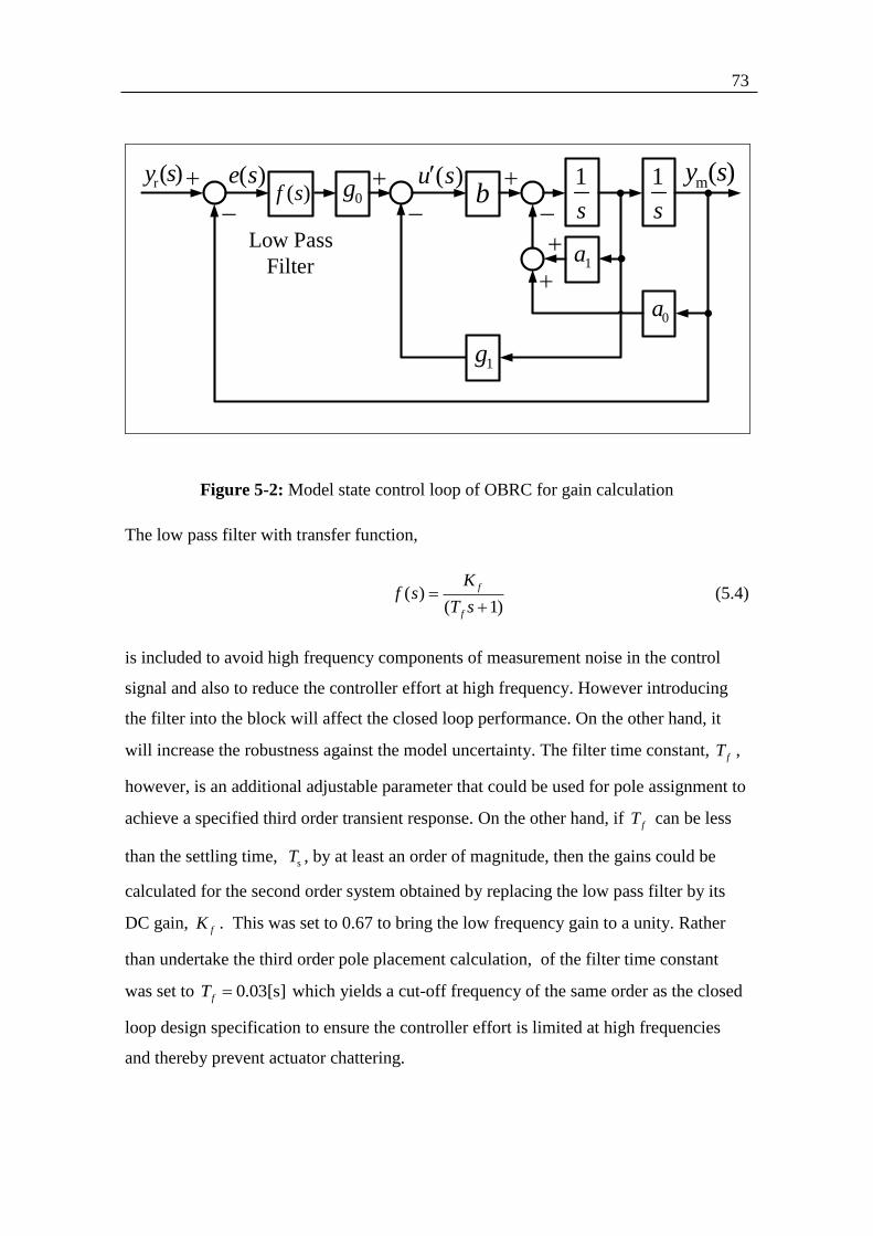
73
1
s
1
s
1g
1a
0g( )u s
Low Pass
Filter
0a
bm( )y s
( )f s( )e sr( )y s
Figure 5-2: Model state control loop of OBRC for gain calculation
The low pass filter with transfer function,
( )( 1)
f
f
Kf s
T s
(5.4)
is included to avoid high frequency components of measurement noise in the control
signal and also to reduce the controller effort at high frequency. However introducing
the filter into the block will affect the closed loop performance. On the other hand, it
will increase the robustness against the model uncertainty. The filter time constant, fT ,
however, is an additional adjustable parameter that could be used for pole assignment to
achieve a specified third order transient response. On the other hand, if fT can be less
than the settling time, sT , by at least an order of magnitude, then the gains could be
calculated for the second order system obtained by replacing the low pass filter by its
DC gain, fK . This was set to 0.67 to bring the low frequency gain to a unity. Rather
than undertake the third order pole placement calculation, of the filter time constant
was set to 0.03[s]fT which yields a cut-off frequency of the same order as the closed
loop design specification to ensure the controller effort is limited at high frequencies
and thereby prevent actuator chattering.
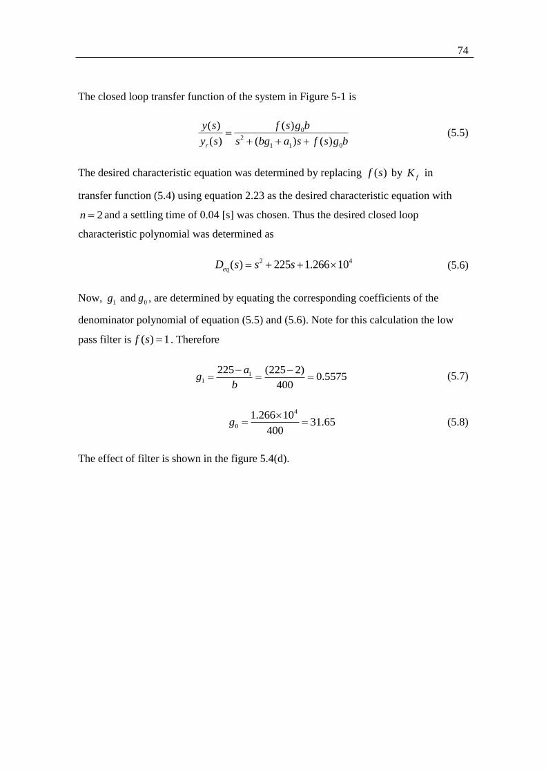
74
The closed loop transfer function of the system in Figure 5-1 is
0
2
1 1 0
( ) ( )
( ) ( ) ( )r
y s f s g b
y s s bg a s f s g b
(5.5)
The desired characteristic equation was determined by replacing ( )f s by fK in
transfer function (5.4) using equation 2.23 as the desired characteristic equation with
2n and a settling time of 0.04 [s] was chosen. Thus the desired closed loop
characteristic polynomial was determined as
2 4( ) 225 1.266 10eqD s s s (5.6)
Now, 1g and 0g , are determined by equating the corresponding coefficients of the
denominator polynomial of equation (5.5) and (5.6). Note for this calculation the low
pass filter is ( ) 1f s . Therefore
11
225 (225 2)0.5575
400
ag
b
(5.7)
4
0
1.266 1031.65
400g
(5.8)
The effect of filter is shown in the figure 5.4(d).
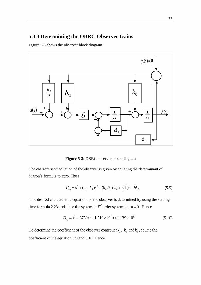
75
5.3.3 Determining the OBRC Observer Gains
Figure 5-3 shows the observer block diagram.
ˆ ( )ey s1
s
( ) 0ey s
( )u s b
1
s
0k1k2k
s
0a
1a
Figure 5-3: OBRC observer block diagram
The characteristic equation of the observer is given by equating the determinant of
Mason’s formula to zero. Thus
3 2
1 0 0 1 0 1 2ˆ ˆˆ ˆ ˆ(a ) (k b)eqC s k s a a k s bk (5.9)
The desired characteristic equation for the observer is determined by using the settling
time formula 2.23 and since the system is 3rd
order system i.e. 3n . Hence
3 2 7 106750 1.519 10 1.139 10eqD s s s (5.10)
To determine the coefficient of the observer controller 2k , 1k and 0k , equate the
coefficient of the equation 5.9 and 5.10. Hence

76
10 10
2
1.139 10 1.139 1028475000
ˆ 400k
b
(5.11)
7 7 7
0 1 01
ˆ ˆ1.519 10 (k ) 1.519 10 (1.519 10 2 400)
ˆ 400b
a ak
1 -37976k (5.11a)
7 7
0 11.519 10 (1.519 10 2) 15189998k a (5.12)
5.3.4 Cascade Controller equivalent to OBRC
To allow us to compare the OBRC controller in the frequency domain, we will
determine the OBRC controller by creating an equivalent closed loop block diagram
with unity feedback. Hence
( ( ))
( )(1 ( ))
obrccl
obrc
K P sG s
K P s
(5.13)
where ( )obrcK s Is the equivalent transfer function of the OBRC controller and ( )P s is
the plant with transfer function given by equation 5.2. Re-arranging (5.9) and making
the “ obrcK ” the subject yields
( ( ))
( )( ( ) ( ) ( ))
clobrc
cl
G sK s
P s G s P s
(5.14)
Therefore
( ) ( )o obrcL s K P s
1
(1 )oS
L
1
(1 )o
o
TS
Hence, the following equations are derived from the closed loop transfer function using
the above relationship.
3 2 7
4 5 3 9 2 11 9
282656.25( 9002 180400 3.6 10 )( )
( 1.8 10 8.106 10 2.7 10 1.2 10 )obrc
s s sK s
s s s s
(5.15)
4 2 2
4 2 2 2
( 150)( 9 10 ) ( 0.004444)( 2 400)
( 9 10 ) ( 149.9 5626)( 2 400)o
s s s s sS
s s s s s
(5.16)

77
11 9 9 4 2
4 2 2
1.0904 10 ( 5.452 10 )( 5.452 10 )( 7.2 10 )( 2 400)
(( 7.2 10 ) ( 108.4)( 41.5)( 2 400))o
s s s s sT
s s s s s
(5.17)
The closed loop transfer functions of the system for the OBRC and H-infinity is given
by equations (5.18) and (5.19) respectively
4 2
202499999.9997
( 9 10 )( 61.98 2250)clobrcG
s s s
(5.18)
4
inf 4 2 2
119092918.5615( 2.095 10 )( 6200)
( 2.095 10 ) ( 6199)( 146.4 5737)H
s sG
s s s s
(5.19)
The closed equation of system with no filter
4
5062500
( 8.995 10 )( 56.29)clNofilterG
s s
(5.20)
Figure 5-4 shows comparisons in the time and frequency domains.
10-2
100
102
104
106
-40
-20
0
20
40
60
80
100
Magnitu
de (
dB
)
Comparison of H-inf and OBRC Controller
Frequency (rad/s)
OBRC |KS|
H-inf|KS|
(a) (b)
(c) (d)
0 0.02 0.04 0.06 0.08 0.1 0.12 0.14 0.160
0.1
0.2
0.3
0.4
0.5
0.6
0.7
0.8
0.9
1
Comparison of H-inf and OBRC Step Response
Time [Sec]
Am
plit
ude[A
rbitra
ry U
nit]
Step
OBRC
H-inf
10-2
100
102
104
106
-80
-60
-40
-20
0
20
40
Magnitu
de (
dB
)
Comparison of H-inf and OBRC Sensitivity equation
Frequency (rad/s)
OBRC
H-inf
|W1|
10-2
100
102
104
106
-30
-20
-10
0
10
20
30
Magnitu
de (
dB
)
Comparison of H-inf and OBRC Controller
Frequency (rad/s)
OBRC |KS|
H-inf|KS|
Figure 5-4: OBRC and Hclosed loop response
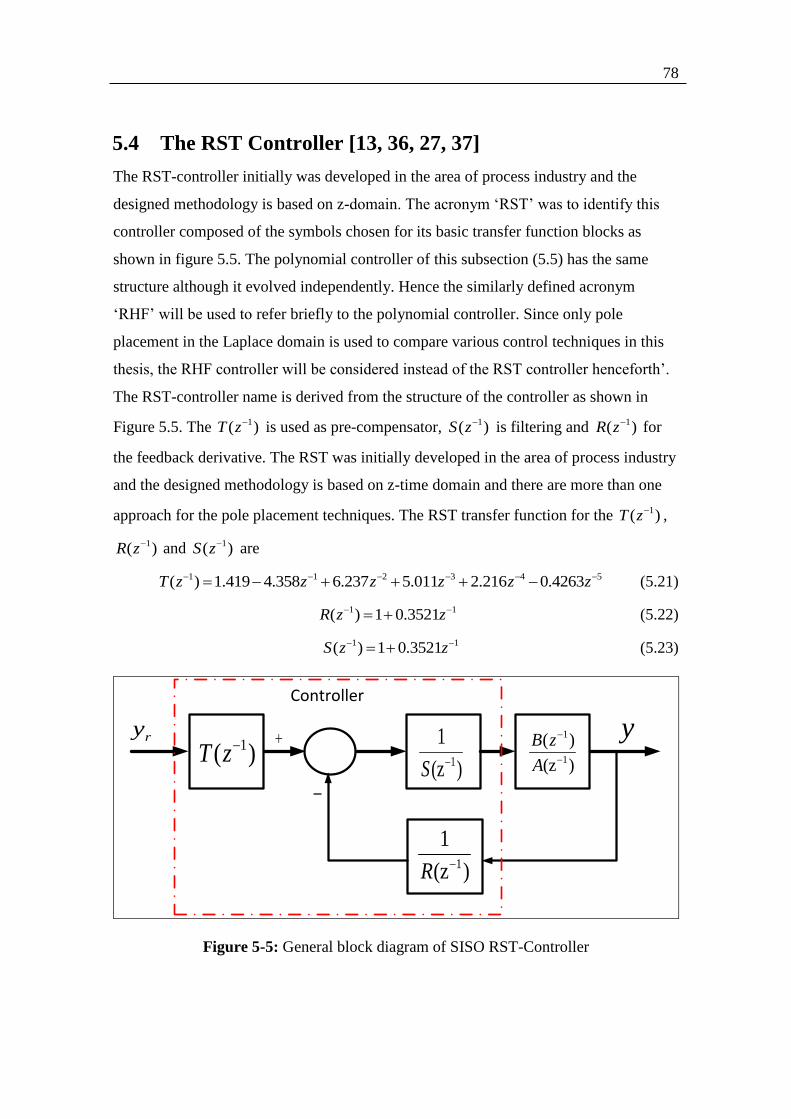
78
5.4 The RST Controller [13, 36, 27, 37]
The RST-controller initially was developed in the area of process industry and the
designed methodology is based on z-domain. The acronym ‘RST’ was to identify this
controller composed of the symbols chosen for its basic transfer function blocks as
shown in figure 5.5. The polynomial controller of this subsection (5.5) has the same
structure although it evolved independently. Hence the similarly defined acronym
‘RHF’ will be used to refer briefly to the polynomial controller. Since only pole
placement in the Laplace domain is used to compare various control techniques in this
thesis, the RHF controller will be considered instead of the RST controller henceforth’.
The RST-controller name is derived from the structure of the controller as shown in
Figure 5.5. The 1( )T z is used as pre-compensator, 1( )S z is filtering and 1( )R z for
the feedback derivative. The RST was initially developed in the area of process industry
and the designed methodology is based on z-time domain and there are more than one
approach for the pole placement techniques. The RST transfer function for the 1( )T z ,
1( )R z and 1( )S z are
1 1 2 3 4 5( ) 1.419 4.358 6.237 5.011 2.216 0.4263T z z z z z z (5.21)
1 1( ) 1 0.3521R z z (5.22)
1 1( ) 1 0.3521S z z (5.23)
1
1
( )
(z )
B z
A
1
1
(z )S
1
1
(z )R
1( )T zyry
Controller
Figure 5-5: General block diagram of SISO RST-Controller
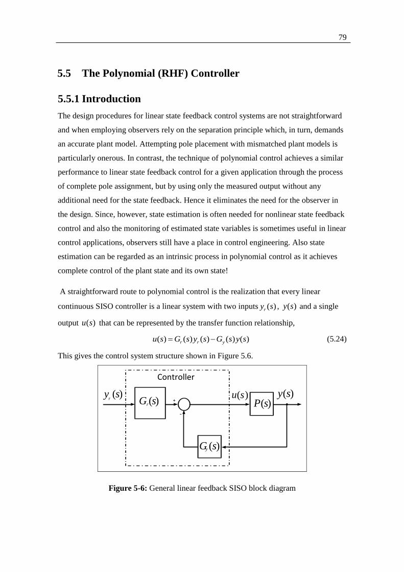
79
5.5 The Polynomial (RHF) Controller
5.5.1 Introduction
The design procedures for linear state feedback control systems are not straightforward
and when employing observers rely on the separation principle which, in turn, demands
an accurate plant model. Attempting pole placement with mismatched plant models is
particularly onerous. In contrast, the technique of polynomial control achieves a similar
performance to linear state feedback control for a given application through the process
of complete pole assignment, but by using only the measured output without any
additional need for the state feedback. Hence it eliminates the need for the observer in
the design. Since, however, state estimation is often needed for nonlinear state feedback
control and also the monitoring of estimated state variables is sometimes useful in linear
control applications, observers still have a place in control engineering. Also state
estimation can be regarded as an intrinsic process in polynomial control as it achieves
complete control of the plant state and its own state!
A straightforward route to polynomial control is the realization that every linear
continuous SISO controller is a linear system with two inputs ( )ry s , ( )y s and a single
output ( )u s that can be represented by the transfer function relationship,
( ) ( ) ( ) ( ) ( )r r yu s G s y s G s y s (5.24)
This gives the control system structure shown in Figure 5.6.
+
-
)(sy
Controller
)(sGr
)(sGy
)(sP)(su)(sy
r
Figure 5-6: General linear feedback SISO block diagram
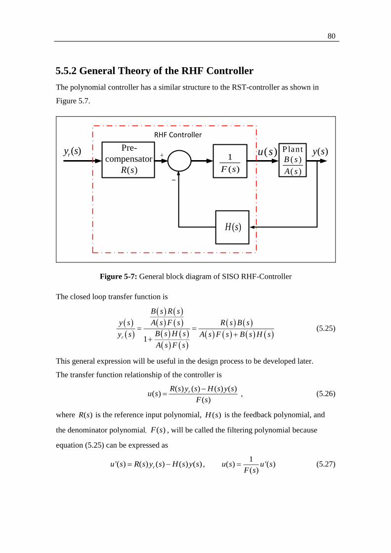
80
5.5.2 General Theory of the RHF Controller
The polynomial controller has a similar structure to the RST-controller as shown in
Figure 5.7.
RHF Controller
1
( )F s
( )H s
Pre-
compensator
( )R s
( )y s( )ry s Plant
( )
( )
B s
A s
( )u s
Figure 5-7: General block diagram of SISO RHF-Controller
The closed loop transfer function is
1r
B s R s
y s A s F s R s B s
B s H sy s A s F s B s H s
A s F s
(5.25)
This general expression will be useful in the design process to be developed later.
The transfer function relationship of the controller is
( ) ( ) ( ) ( )
( )( )
rR s y s H s y su s
F s
, (5.26)
where ( )R s is the reference input polynomial, ( )H s is the feedback polynomial, and
the denominator polynomial, ( )F s , will be called the filtering polynomial because
equation (5.25) can be expressed as
'( ) ( ) ( ) ( ) ( )ru s R s y s H s y s , 1
( ) '( )( )
u s u sF s
(5.27)

81
in which any amplified high frequency components of measurement noise in '( )u s due
to the derivative action of ( )H s is attenuated before reaching the controller output ( )u s ,
due to the low pass filtering action of the transfer function 1
( )F s. This is equivalent to
the filtering provided by an observer in a linear state feedback controller. It is clear that
( )R s is an external pre-compensator and the pre-compensator can be designed
independently of the closed loop part. It also provides a means compensating the effect
of the plant zeros without reducing the sensitivity if a further polynomial, ( )Z s , is
introduced as the denominator of the reference input transfer function, by replacing
(5.26) with the following:
1 ( )
( ) ( ) ( ) ( )( ) ( )
r
R su s y s H s y s
F s Z s
(5.28)
The design procedure assumes the general plant transfer function is expressed in terms
of its numerator and denominator polynomials, ( )A s and ( )B s , which are respectively
1
0
( )an
na i
i
i
A s s a s
and
1
0
( )bn
i
i
i
B s b s
. (5.29)
Also the relative degree of the open loop system has to be greater than zero to avoid an
algebraic loop. Hence a bn n . Later on an example of zero relative degree ( a bn n )
will be used to present a procedure to handle this type of system.
Similarly, the controller polynomials are expressed as
1 1
0 0
1 1
0 0
( ) ( )
( ) ( )
h f
z r
n ni i
i ii i
n ni i
i ii i
H s h s F s f s
Z s z s R s r s
(5.30)
The coefficients of the polynomials, ( )H s and ( )F s , are the adjustable controller
parameters used for the pole placement, the number of which can be minimised for
given polynomial degrees. This allows the minimum order of closed loop system to be
achieved for a given plant. The pre-compensator numerator polynomial is not

82
normalized in order to provide 1rn coefficients, enabling its rn zeros to be placed
independently and the required closed loop DC gain to be set, which is usually unity.
The functions of the polynomial controller terms are defined in Table 5.1.
Table 5.1: The RHF-controller functions
Components Purpose
( )H s To provide a sufficient number of adjustable coefficients in the controller
to enable complete pole placement
1
( )F s
To prevent high frequency components of measurement noise amplified
by ( )H s appearing as ( )u s
( )Z s To act as an external zero pre-compensator when needed, otherwise
being set to unity
( )R s To cancel some or all of the closed loop poles if desirable, otherwise
00 ( )rn R s r to become a simple reference input scaling coefficient
5.5.3 Constraints on Polynomial Degrees
With reference to the general closed loop transfer function (5.25), the closed loop
characteristic polynomial is
A s F s B s H s . (5.31)
Hence the order of the closed loop part of the system, excluding the pre-compensator, is
( ), ( )a f b hN MAX n n n n (5.32)
Importantly, the closed loop system cannot contain an algebraic loop. This is guaranteed
if the relative degree of the open loop transfer function is positive. Thus,
( ) ( )
Reldeg ( ) 0( ) ( )
a f b h
B s H sn n n n
A s F s
(5.33)
It then follows from (5.32) and (5.33) that the total system order is
a fN n n (5.34)
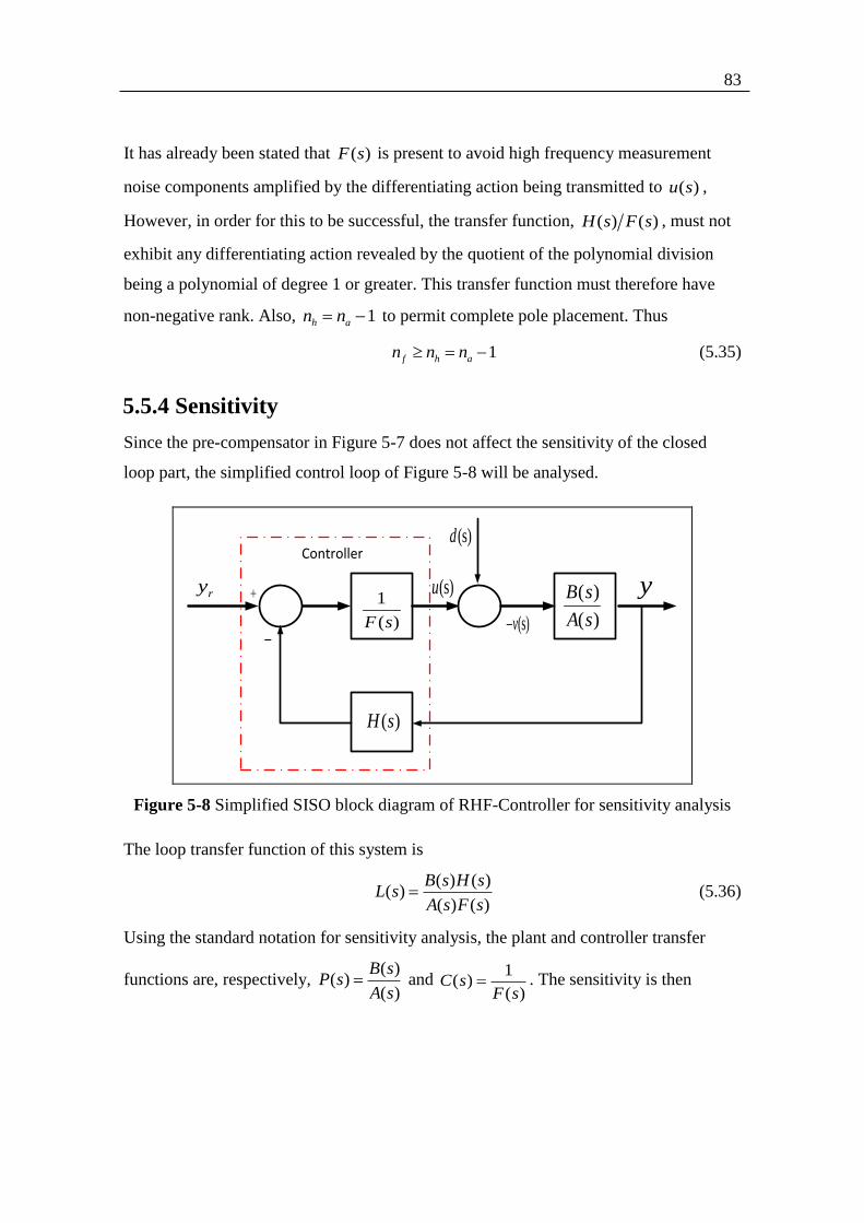
83
It has already been stated that ( )F s is present to avoid high frequency measurement
noise components amplified by the differentiating action being transmitted to ( )u s ,
However, in order for this to be successful, the transfer function, ( ) ( )H s F s , must not
exhibit any differentiating action revealed by the quotient of the polynomial division
being a polynomial of degree 1 or greater. This transfer function must therefore have
non-negative rank. Also, 1h an n to permit complete pole placement. Thus
1f h an n n (5.35)
5.5.4 Sensitivity
Since the pre-compensator in Figure 5-7 does not affect the sensitivity of the closed
loop part, the simplified control loop of Figure 5-8 will be analysed.
yry
Controller
1
( )F s
( )H s
(s)d
(s)u
(s)v
( )
( )
B s
A s
Figure 5-8 Simplified SISO block diagram of RHF-Controller for sensitivity analysis
The loop transfer function of this system is
( ) ( )
( )( ) ( )
B s H sL s
A s F s (5.36)
Using the standard notation for sensitivity analysis, the plant and controller transfer
functions are, respectively, ( )
( )( )
B sP s
A s and
1( )
( )C s
F s . The sensitivity is then

84
1 1 ( ) ( )
( )( ) ( )1 ( ) ( ) ( ) ( ) ( ) ( ) ( )1( ) ( )
A s F sS s
B s H sC s P s H s A s F s B s H s
A s F s
(5.37)
The same result can be obtained directly from Figure 5-8 as the transfer function
between the net plant input, ( )v s , and the disturbance input, ( )d s . Thus
( ) 1
( )( ) ( )( ) 1( ) ( )
v sS s
B s H sd s
A s F s
Hence, the sensitivity for the RHF-controller is given by
( ) ( )
( )( ) ( ) ( ) ( )
A s F sS s
A s F s B s H s
. (5.38)
5.5.5 Derivation of the General Pole Placement Equation
For pole placement of the closed loop system, the characteristic polynomial (5.31) will
be set equal to a specified polynomial, ( )D s , formed from the required closed loop pole
locations. Thus
( ) ( ) ( ) ( ) ( )A s F s B s H s D s . (5.39)
A general algorithm for calculating the coefficients of ( )H s and ( )F s with a plant of
arbitrary order will now be developed. The starting point will be the general linear
second order plant with transfer function,
1 0
2
1 0
( )
( )
b s by s
u s s a s a
. (5.40)
The result obtained with this will enable the general pole placement equation to be
deduced. The characteristic polynomial of (5.39) will be divided into two components,
( ) ( )A s F s and ( ) ( )B s H s , as follows.
2 2 2
1 0 2 1 0 2 1 0 1 0( ) ( ) ( ) ( ) ( )( ) ( )( )iA s F s B s H s s a s a f s f s f k h s h s h b s b
Consider first the ( ) ( )A s F s component,
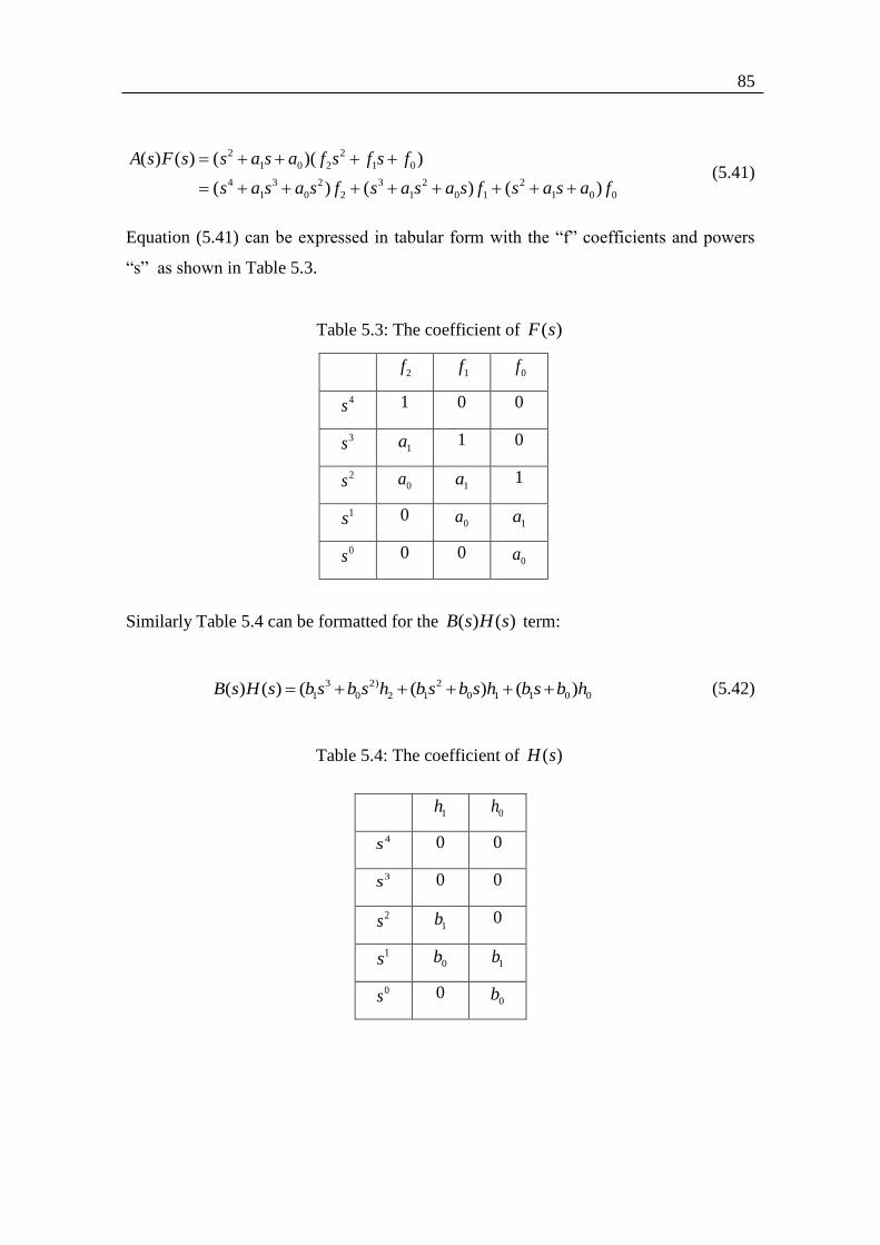
85
2 2
1 0 2 1 0
4 3 2 3 2 2
1 0 2 1 0 1 1 0 0
( ) ( ) ( )( )
( ) ( ) ( )
A s F s s a s a f s f s f
s a s a s f s a s a s f s a s a f
(5.41)
Equation (5.41) can be expressed in tabular form with the “f” coefficients and powers
“s” as shown in Table 5.3.
Table 5.3: The coefficient of ( )F s
2f 1f 0f
4s 1 0 0
3s 1a 1 0
2s 0a 1a 1
1s 0 0a 1a
0s 0 0 0a
Similarly Table 5.4 can be formatted for the ( ) ( )B s H s term:
3 2) 2
1 0 2 1 0 1 1 0 0( ) ( ) ( ( ) ( )B s H s b s b s h b s b s h b s b h (5.42)
Table 5.4: The coefficient of ( )H s
1h 0h
4s 0 0
3s 0 0
2s 1b 0
1s 0b 1b
0s 0 0b

86
Combining Tables 5.3 and 5.4 yields Table 5.5 that contains the “f” and “h”
coefficients.
Table 5.5: The Augmenting of the ( )F s and ( )H s Coefficients
2f
1f 0f
1h 0h
4s 1 0 0 0 0
3s 1a 1 0 0 0
2s 0a 1a 1 1b 0
1s 0 0a 1a 0b 1b
0s 0 0 0a 0
0b
Then by observation of this table, the following linear matrix equation may be written.
2
1 3
0 2
0 1 1
0 1 0 1
1 1
0 0
0 0
11 0 0 0 0
1 1 0 0 0
1 0
0
0 0 0
f
f da
f da a b
a a b bh d
a bh d
MK D
(5.43)
where M is the plant parameter matrix, D is the coefficient vector of the desired
characteristic equation and K is the vector of controller parameters comprising the filter
coefficients and feedback gains. Equation (5.53) is solved for K. Hence, later on the
robustness controllers will be compared.

87
5.5.6 Basic RHF Controller Example
The design of the pre-compensator with reference input,r ( )y s and output,
r ( )y s is
separate from the main RHF control loop and is considered in the following subsection.
The closed loop system block diagram is shown in Figure 5.14 for plant (5.1).
(s)u y(s)
2
2 1 0
1
f s f s f
2
2 1 0h s h s h
0
3127( )
3
s b
s
r ( )y s
Figure 5-9: Closed loop system for RHF design
The general form of the characteristic equation obtained with this loop structure is
( ) ( ) ( ) ( ) 0A s F s H s B s . In this particular case it is
3 2 2
2 1 0 2 1 0 0
127( ) ( ) ( )( )
3s f s f s f h s h s h s b (5.44)
To determine the controller parameters using the settling time formula (2.23), there are
two options. The first is to place all five closed loop poles at one point. The second
option is robust pole placement in which the closed loop poles are split into two groups,
one dominant group at one location and the other at another location with a much larger
magnitude to give additional robustness. With plant uncertainty, however, there is a
trade-off between the robustness and stability. In robust pole placement, the desired
characteristic equation is reformulated and is given by
Dominant Mode Fast mode for robustness
( )( )
1.5( 1) 1.5( 1)( )
mn
s sf
W sV s
n mD s s s
T T
(5.45)
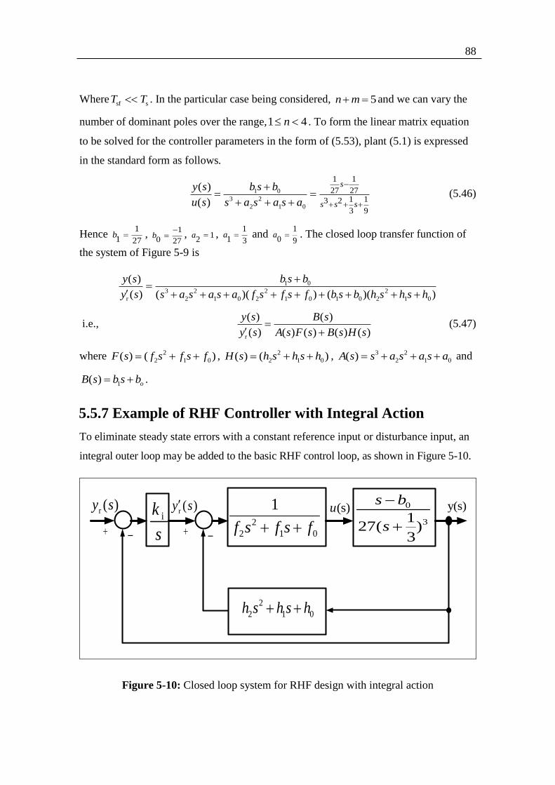
88
Wheresf sT T . In the particular case being considered, 5n m and we can vary the
number of dominant poles over the range,1 4n . To form the linear matrix equation
to be solved for the controller parameters in the form of (5.53), plant (5.1) is expressed
in the standard form as follows.
1 0
3 2
2 1 0
1 1
27 271 13 2
3 9
( )
( )
s
s s s
y s b s b
u s s a s a s a
(5.46)
Hence 1
1 27b ,
1
0 27b
, 1
2a ,
1
1 3a and
1
0 9a . The closed loop transfer function of
the system of Figure 5-9 is
1 0
3 2 2 2
r 2 1 0 2 1 0 1 0 2 1 0
( )
( ) ( )( ) ( )( )
y s b s b
y s s a s a s a f s f s f b s b h s h s h
i.e., r
( ) ( )
( ) ( ) ( ) ( ) ( )
y s B s
y s A s F s B s H s
(5.47)
where 2
2 1 0( ) ( )F s f s f s f , 2
2 1 0( ) ( )H s h s h s h , 3 2
2 1 0( )A s s a s a s a and
1( ) oB s b s b .
5.5.7 Example of RHF Controller with Integral Action
To eliminate steady state errors with a constant reference input or disturbance input, an
integral outer loop may be added to the basic RHF control loop, as shown in Figure 5-10.
(s)u y(s)
2
2 1 0
1
f s f s f
r ( )y s 0
3127( )
3
s b
s
2
2 1 0h s h s h
r ( )y sik
s
Figure 5-10: Closed loop system for RHF design with integral action
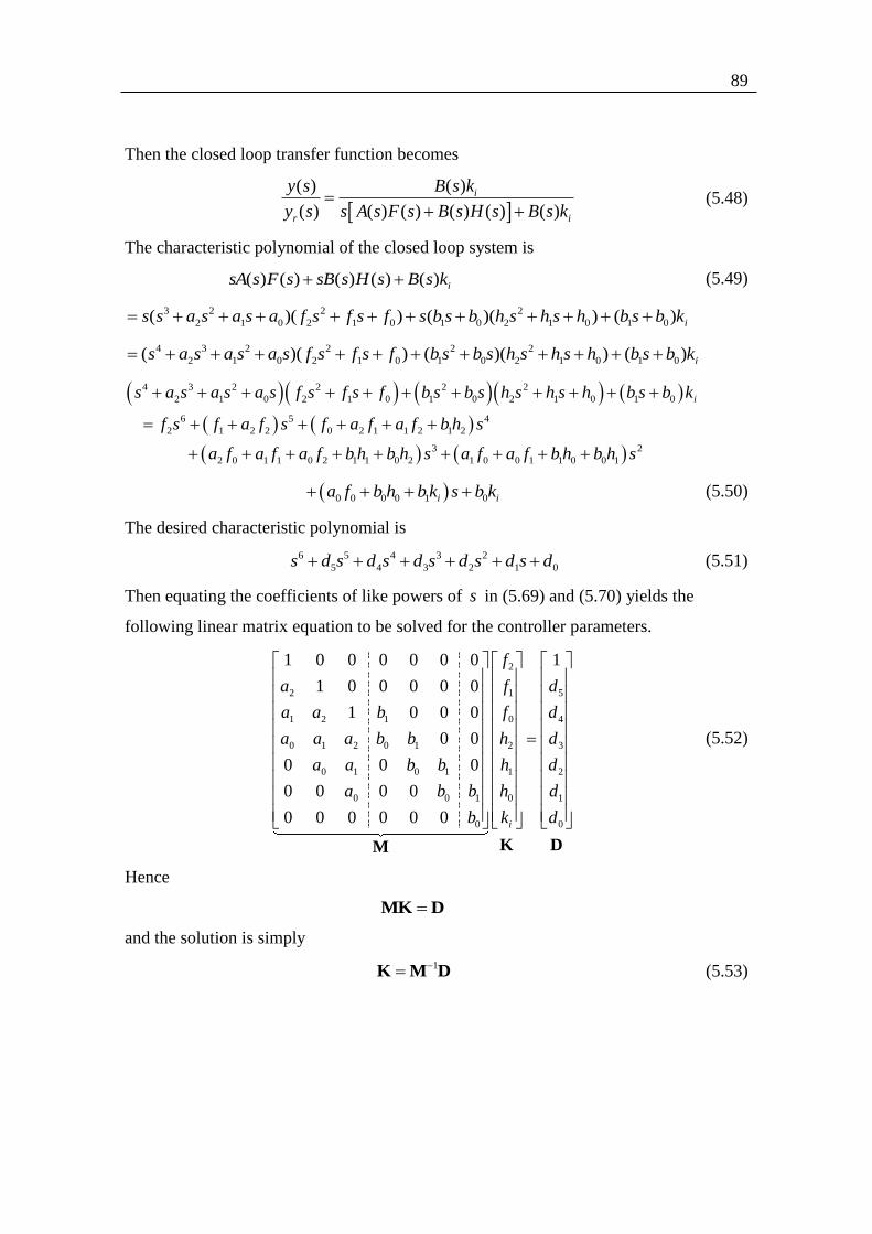
89
Then the closed loop transfer function becomes
( ) ( )
( ) ( ) ( ) ( ) ( ) ( )
i
r i
y s B s k
y s s A s F s B s H s B s k
(5.48)
The characteristic polynomial of the closed loop system is
( ) ( ) ( ) ( ) ( ) isA s F s sB s H s B s k (5.49)
3 2 2 2
2 1 0 2 1 0 1 0 2 1 0 1 0( )( ) ( )( ) ( ) is s a s a s a f s f s f s b s b h s h s h b s b k
4 3 2 2 2 2
2 1 0 2 1 0 1 0 2 1 0 1 0( )( ) ( )( ) ( ) is a s a s a s f s f s f b s b s h s h s h b s b k
4 3 2 2 2 2
2 1 0 2 1 0 1 0 2 1 0 1 0
6 5 4
2 1 2 2 0 2 1 1 2 1 2
3 2
2 0 1 1 0 2 1 1 0 2 1 0 0 1 1 0 0 1
is a s a s a s f s f s f b s b s h s h s h b s b k
f s f a f s f a f a f b h s
a f a f a f b h b h s a f a f b h b h s
0 0 0 0 1 0i ia f b h b k s b k (5.50)
The desired characteristic polynomial is
6 5 4 3 2
5 4 3 2 1 0s d s d s d s d s d s d (5.51)
Then equating the coefficients of like powers of s in (5.69) and (5.70) yields the
following linear matrix equation to be solved for the controller parameters.
2
2 1 5
1 2 1 0 4
0 1 2 0 1 2 3
0 1 0 1 1 2
0 0 1 0 1
0 0
1 0 0 0 0 0 0 1
1 0 0 0 0 0
1 0 0 0
0 0
0 0 0
0 0 0 0
0 0 0 0 0 0 i
f
a f d
a a b f d
a a a b b h d
a a b b h d
a b b h d
b k d
K DM
(5.52)
Hence
MK D (5.77)
and the solution is simply
1K M D (5.53)
90
5.5.8 Pre-compensator
The pre-compensator is not necessary in this case, because the poles of the closed loop
system are chosen to reduce the effect of the zero to acceptable proportions during the
transient. In subsections 5.9.5 and 5.9.6, however, performance comparisons are made
with and without a pre-compensator to further reduce the effect of the zero. This pre-
compensator consists of a rd3 order low pass filter was used as a pre-compensator with
a step response settling time of 0.1[s]soT , the filtering time constant being 6soT .
5.5.9 Sine Wave Oscillator Example
This is another example that illustrates the capability of the RHF-controller. It was used
in paper [37] and the original plant model was given in the z-domain as shown in Figure
5.3, an RST controller being applied. The initial step was to convert from the z-domain
to the s-domain using Tustin’s approximation, resulting in the plant transfer function,
2
2
( ) 0.7692 61.54 923.1
( ) ( 10.77 )
y s s s
u s s s
. (5.54)
This, however, has zero relative degree, implying that the RHF-controller cannot be
used directly but this problem was solved by inserting a pure integrator in the plant
input. Also the integrator will bring the benefits of a) acting as a low pass filter and
attenuating high frequency components of measurement noise before they reach the
physical plant input, and b) ensuring zero steady state error for any constant external
disturbance components referred to the control input. Although this integrator is an
addition to the controller, it is treated as part of the plant for the purpose of determining
the controller parameters. So the task is to design an RHF controller for the augmented
plant that has the transfer function,
2 2
2 1 0
2 3 2
2 1 0
( ) 0.7692 61.54 923.1
( ) ( 10.77 )
y s s s b s b s b
u s s s s s a s a s a
, (5.55)
and therefore a relative degree of 1, where the physical plant input is 1
( ) ( )u s u ss .
According to (5.48) and (5.49), the minimum order the system can have is a fN n n
2 1 5an . So the matrix, M , is of dimension 1 1 6 6N N . Thus
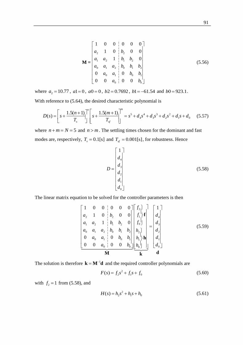
91
2 2
1 2 1 2
0 1 2 0 1 2
0 1 0 1
0 0
1 0 0 0 0 0
1 0 0 0
1 0
0 0
0 0 0 0
a b
a a b b
a a a b b b
a a b b
a b
M = (5.56)
where 2 10.77a , 1 0a , 0 0a , 2 0.7692b , 1 61.54b and 0 923.1b .
With reference to (5.64), the desired characteristic polynomial is
5 4 3 2
4 3 2 1 0
1.5( 1) 1.5( 1)( )
mn
s sf
n mD s s s s d s d s d s d s d
T T
(5.57)
where 5n m N and n m . The settling times chosen for the dominant and fast
modes are, respectively, 0.1[s]sT and 0.001[s]sfT , for robustness. Hence
4
3
2
1
0
1
d
dD
d
d
d
(5.58)
The linear matrix equation to be solved for the controller parameters is then
2
12 2 4
01 2 1 2 3
0 1 2 0 1 2 22
0 1 0 1 11
0 0 00
1 0 0 0 0 0 1
1 0 0 0
1 0
0 0
0 0 0 0
f
fa b d
fa a b b d
a a a b b b dh
a a b b dh
a b dh
f
h
dM k
(5.59)
The solution is therefore 1k M d and the required controller polynomials are
2
2 1 0( )F s f s f s f (5.60)
with 2 1f from (5.58), and
2
2 1 0( )H s h s h s h (5.61)
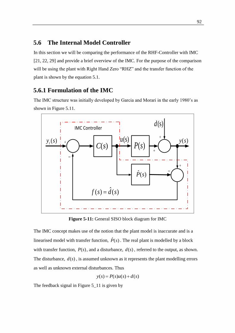
92
5.6 The Internal Model Controller
In this section we will be comparing the performance of the RHF-Controller with IMC
[21, 22, 29] and provide a brief overview of the IMC. For the purpose of the comparison
will be using the plant with Right Hand Zero “RHZ” and the transfer function of the
plant is shown by the equation 5.1.
5.6.1 Formulation of the IMC
The IMC structure was initially developed by Garcia and Morari in the early 1980’s as
shown in Figure 5.11.
IMC Controller(s)d
(s)u( )P s
ˆ( )P s
( )y sr ( )y s
( )C s
ˆ( ) ( )f s d s
Figure 5-11: General SISO block diagram for IMC
The IMC concept makes use of the notion that the plant model is inaccurate and is a
linearised model with transfer function, ˆ( )P s . The real plant is modelled by a block
with transfer function, ( )P s , and a disturbance, ( )d s , referred to the output, as shown.
The disturbance, ( )d s , is assumed unknown as it represents the plant modelling errors
as well as unknown external disturbances. Thus
( ) ( ) ( ) ( )y s P s u s d s
The feedback signal in Figure 5_11 is given by

93
ˆ ˆ( ) ( ) ( ) ( ) ( ) ( ) ( ) ( ) ( ) ( )f s P s u s d s P s u s P s P s u s d s
Since ( ) ( )f s d s if ˆ( ) ( )P s P s , then ( )f s may be regarded as a disturbance
estimate, ˆ( )d s . It is evident by inspection of Figure 5-11 that if 1ˆ( ) ( )C s P s and
ˆ( ) ( )P s P s , then the feedback signal will precisely cancel the disturbance, ( )d s .
However in reality, the plant model is not a perfect match and therefore ( )d s will be a
combination of the plant uncertainty and disturbance [3]. Nevertheless with ˆ( ) ( )P s P s ,
a degree of disturbance cancellation would be expected and therefore the control loop
structure shown should have considerable robustness.
The closed loop transfer function of Figure 5.11 is
ˆ( ) ( ) ( ) 1 ( ) ( ) ( )
( )ˆ1 ( ) ( ) ( )
rC s P s y s C s P s d sy s
P s P s C s
(5.62)
It is evident that if 1ˆ( ) ( )C s P s , and ˆ( ) ( )P s P s then r
( )1
( )
y s
y s , which implies
perfect tracking of the set point and disturbance rejection. Although in practice,
ˆ( ) ( )P s P s since the plant model cannot perfectly match the actual plant, a perfect
disturbance rejection can still be achieved by adjusting ( )C s until 1ˆ( ) ( )C s P s . Then
to achieve acceptable robustness of the closed loop system, we must ensure that the
estimated model is closely matched to the real plant as possible. In general the model
mismatch will be more pronounced at the higher frequencies. Hence, a low pass filter
with transfer function, ( )fC s , is required in series with the controller, yielding a net
controller transfer function of imc( ) ( ) ( )fC s C s C s . This also attenuates the noise
caused by the derivative action of the controller, due to the inversion of the transfer
function of the plant and mismatch of the model. Clearly in practice the plant is not
always invertible and hence, the plant model can be divided into components, one
which is invertible and another which is non-invertible, respectively ( )P s and ( )P s ,
and then setting 1
( )C s P s
.

94
5.6.2 Sensitivity
For the purpose of sensitivity analysis, Figure 5-12 shows the unity feedback version of
the IMC loop. It may be readily shown that its closed loop transfer function is the same
as that of Figure 5-11.
IMC Controller (s)d
(s)u( )P s
ˆ( )P s
( )e s( )C s
( )y sr( )y s
Figure 5-12: IMC block diagram with unity feedback
The sensitivity transfer function is
ˆ1
ˆ1
y s C s P sS s
d s C s P s P s
Remarkably, since P s is known precisely, then provided it is feasible to set
1ˆ( ) ( )C s P s , then the sensitivity will be zero, implying ideal robustness. As pointed
out in the previous subsection, however, this inversion is only possible for a factor of
( )P s in many cases.

95
5.6.3 Design Procedure
Step 1: Split the transfer function into two components “invertible and non-invertible”
Step 2: Determine the open loop response of the plant.
Step 3: Design the controller transfer function as shown in equation 5.63
1
imc
( )( )
(1 )n
f
P sC s
s
(5.63)
where n is the order of the filter and f is the time constant of filter. The bandwidth of
the filter needs to be twice the bandwidth of the open loop plant.
The IMC controller was designed using the Matlab SISO Tool and the controller is
3
imc 2
19.3205( 0.333)( )
( 2.709 3.17)
sC s
s s s
(5.64)
(s)u y(s)y ( )r s
0
3
Plant model
127
3
s b
s
3
2
19.3205 (s 0.333)
(s 2.709s 3.17)s
Real Plant
IMC Controller
Figure 5-13 Block diagram of SISO IMC system

96
5.7 The H-Infinity Controller
5.7.1 Overview
The H-infinity control theory is well documented in [12, 45] and some further reading
material can also be found in [45, 51, 41]. Hence this section concentrates on its
application. The H-infinity methodology is based on a complex optimisation procedure
and one must use an off-the-shelf software package to design the controller. The
designer has to formulate a constraint based on the desired performance.
In this section, a design for plant (5.2) will be produced.
5.7.2 Formulation of the H-infinity Controller
The structure of the H-infinity control loop is the simple classical unity feedback one, as
shown in Figure 5-14.
(s)u( )P s( )K s
y(s)y ( )r s
Figure 5-14: H-infinity Block diagram without constraints
The sophistication is in the determination of the controller transfer function, ( )K s .
The key steps for the designer are to understand the plant, beware of the tool pitfalls,
and be able to formulate the design specification into the weighting function which is
then used as a constraint in the software tool. Table 5.6 presents a specification, and the
terms of which are explained in the following subsection.

97
Table 5.6: Typical design specification
Controlparameter Requirement
ωb The closed loop bandwidth must not excess 35.6 [rad/s]
|KS| The gain must not be greater than 5.5
|Offset| The steady state error must not be greater than 0.01
The optimization must be less than 1.33
5.7.3 Design Specification
In Table 5.6, is the minimisation criteria and the constraints are formed by taking the
transfer function between the disturbance input, ( )d s and outputs 1 2( ), ( ),Z s Z s .
Hence, the minimum constraints for three outputs are
1
2
3
.
min . .
.
W S
W K S
W T
(5.65)
where
1W is the weighting function associated with sensitivity function,
2W is the weighting function associated with sensitivity function and control penalising
high frequency components, and
3W is the weighting function associated with complimentary sensitivity function.
The general block diagram of Figure 5.15 shows the outputs for forming the constraints
for this problem, which will be used by the H-infinity process to design the controller,
( )K s , that meets the design specification and the general form for designing the 1( )W s
and 2 ( )W s . This design specification is given by equation (5.58) and the constraints
plotted on the magnitude as 1
W.
1
/( ) B
B
s MW s
s A
, 3
/( )
B
s B MW s
As
(5.66)
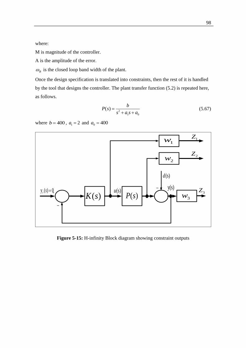
98
where:
M is magnitude of the controller.
A is the amplitude of the error.
B is the closed loop band width of the plant.
Once the design specification is translated into constraints, then the rest of it is handled
by the tool that designs the controller. The plant transfer function (5.2) is repeated here,
as follows.
2
1 0
( )b
P ss a s a
(5.67)
where 400b , 1 2a and 0 400a
(s)d
(s)u( )P s
( )K s
1w
2w
3w3Z
2Z
1Z
y(s)y ( ) 0r s
Figure 5-15: H-infinity Block diagram showing constraint outputs
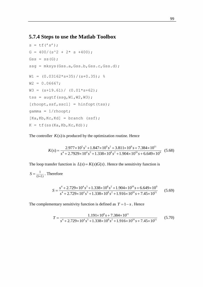
99
5.7.4 Steps to use the Matlab Toolbox
s = tf(’s’);
G = 400/(s^2 + 2* s +400);
Gss = ss(G);
ssg = mksys(Gss.a,Gss.b,Gss.c,Gss.d);
W1 = (0.03162*s+35)/(s+0.35); %
W2 = 0.06667;
W3 = (s+19.61)/ (0.01*s+62);
tss = augtf(ssg,W1,W2,W3);
[rhoopt,ssf,sscl] = hinfopt(tss);
gamma = 1/rhoopt;
[Ka,Kb,Kc,Kd] = branch (ssf);
K = tf(ss(Ka,Kb,Kc,Kd));
The controller ( )K s is produced by the optimization routine. Hence
5 3 9 2 9 11
4 4 3 8 2 10 9
2.977 10 1.847 10 3.811 10 7.384 10( )
2.7929 10 1.338 10 1.904 10 6.649 10
s s sK s
s s s s
(5.68)
The loop transfer function is ( ) ( ) ( )L s K s G s . Hence the sensitivity function is
1
(1 )LS
. Therefore
4 4 3 8 2 10 9
4 4 3 8 2 10 11
2.729 10 1.338 10 1.904 10 6.649 10
2.729 10 1.338 10 1.916 10 7.45 10
s s s sS
s s s s
(5.69)
The complementary sensitivity function is defined as 1T s . Hence
8 11
4 4 3 8 2 10 11
1.191 10 7.384 10
2.729 10 1.338 10 1.916 10 7.45 10
sT
s s s s
(5.70)
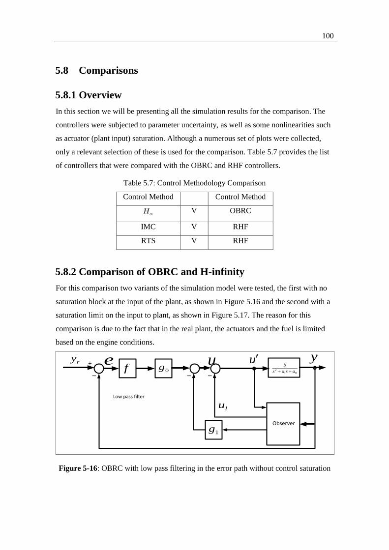
100
5.8 Comparisons
5.8.1 Overview
In this section we will be presenting all the simulation results for the comparison. The
controllers were subjected to parameter uncertainty, as well as some nonlinearities such
as actuator (plant input) saturation. Although a numerous set of plots were collected,
only a relevant selection of these is used for the comparison. Table 5.7 provides the list
of controllers that were compared with the OBRC and RHF controllers.
Table 5.7: Control Methodology Comparison
Control Method Control Method
H V OBRC
IMC V RHF
RTS V RHF
5.8.2 Comparison of OBRC and H-infinity
For this comparison two variants of the simulation model were tested, the first with no
saturation block at the input of the plant, as shown in Figure 5.16 and the second with a
saturation limit on the input to plant, as shown in Figure 5.17. The reason for this
comparison is due to the fact that in the real plant, the actuators and the fuel is limited
based on the engine conditions.
2
1 0
b
s a s a
Observer
f 0g
1g
ry yu u
Low pass filter
lu
e
Figure 5-16: OBRC with low pass filtering in the error path without control saturation

101
ry ymu
2
1 0
b
s a s a
Observer
0g
1g
uu
Low pass filter
e f s
ˆLu
Figure 5-17: OBRC with low pass filtering in the error path with control saturation
Figure 5-18 shows the frequency responses for the low pass filter parameters used.
Figure 5-18: Frequency plot of filters with different time constants
Table 5.8 shows the parameters selected for the H controller.
Table 5.8: Parameters k and n for the H controller
Test k n
1 400 20
2 300 20
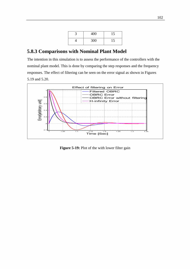
102
3 400 15
4 300 15
5.8.3 Comparisons with Nominal Plant Model
The intention in this simulation is to assess the performance of the controllers with the
nominal plant model. This is done by comparing the step responses and the frequency
responses. The effect of filtering can be seen on the error signal as shown in Figures
5.19 and 5.20.
Figure 5-19: Plot of the with lower filter gain
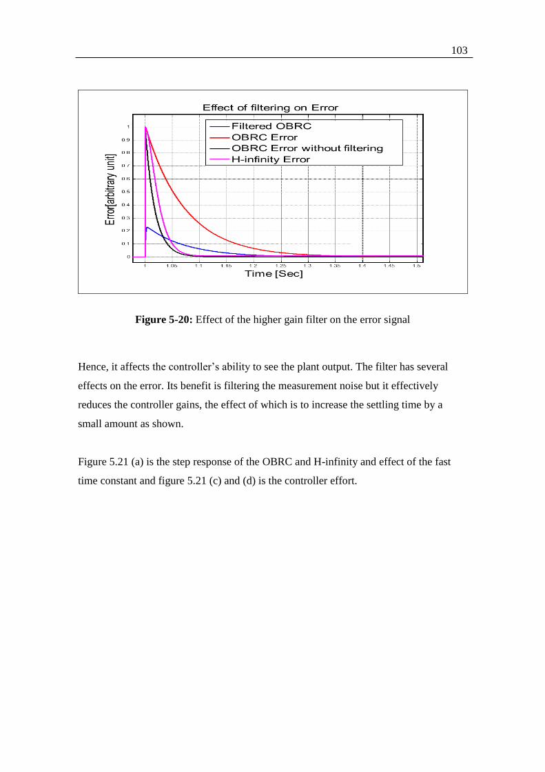
103
Figure 5-20: Effect of the higher gain filter on the error signal
Hence, it affects the controller’s ability to see the plant output. The filter has several
effects on the error. Its benefit is filtering the measurement noise but it effectively
reduces the controller gains, the effect of which is to increase the settling time by a
small amount as shown.
Figure 5.21 (a) is the step response of the OBRC and H-infinity and effect of the fast
time constant and figure 5.21 (c) and (d) is the controller effort.
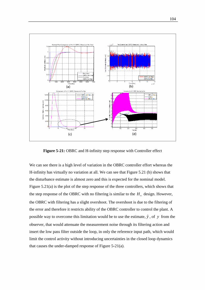
104
Figure 5-21: OBRC and H-infinity step response with Controller effect
We can see there is a high level of variation in the OBRC controller effort whereas the
H-infinity has virtually no variation at all. We can see that Figure 5.21 (b) shows that
the disturbance estimate is almost zero and this is expected for the nominal model.
Figure 5.21(a) is the plot of the step response of the three controllers, which shows that
the step response of the OBRC with no filtering is similar to the H design. However,
the OBRC with filtering has a slight overshoot. The overshoot is due to the filtering of
the error and therefore it restricts ability of the OBRC controller to control the plant. A
possible way to overcome this limitation would be to use the estimate, y , of y from the
observer, that would attenuate the measurement noise through its filtering action and
insert the low pass filter outside the loop, in only the reference input path, which would
limit the control activity without introducing uncertainties in the closed loop dynamics
that causes the under-damped response of Figure 5-21(a).
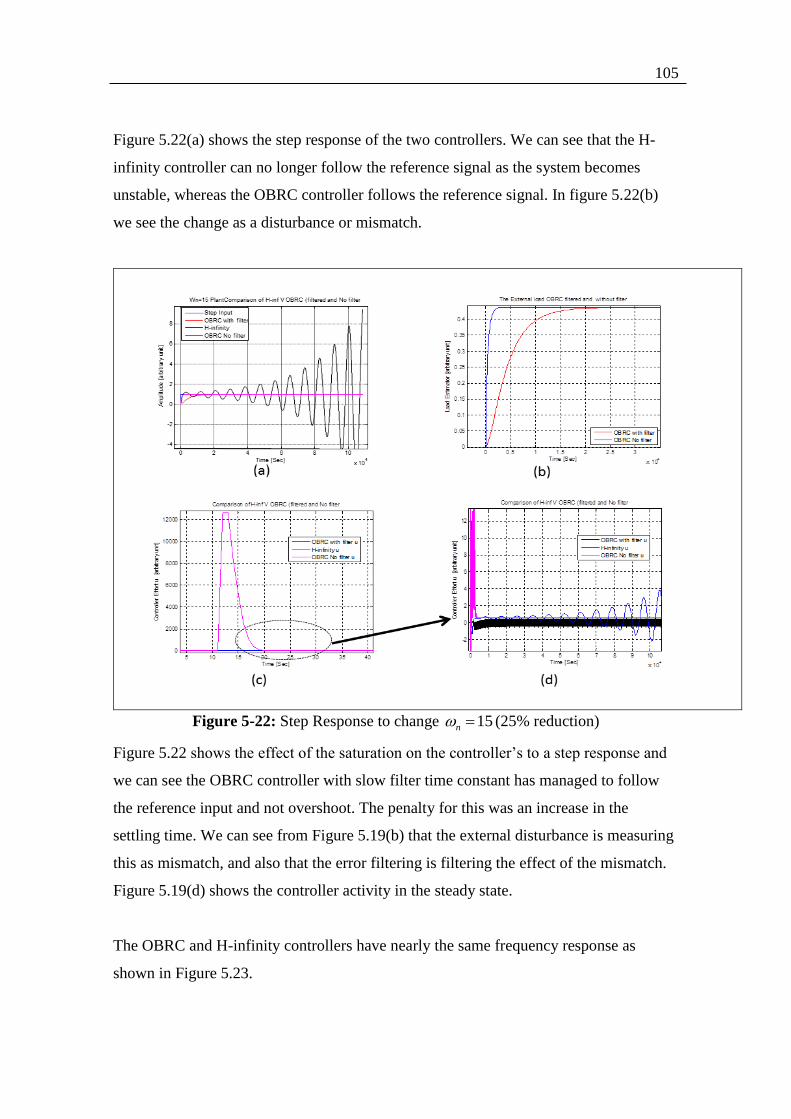
105
Figure 5.22(a) shows the step response of the two controllers. We can see that the H-
infinity controller can no longer follow the reference signal as the system becomes
unstable, whereas the OBRC controller follows the reference signal. In figure 5.22(b)
we see the change as a disturbance or mismatch.
Figure 5-22: Step Response to change 15n (25% reduction)
Figure 5.22 shows the effect of the saturation on the controller’s to a step response and
we can see the OBRC controller with slow filter time constant has managed to follow
the reference input and not overshoot. The penalty for this was an increase in the
settling time. We can see from Figure 5.19(b) that the external disturbance is measuring
this as mismatch, and also that the error filtering is filtering the effect of the mismatch.
Figure 5.19(d) shows the controller activity in the steady state.
The OBRC and H-infinity controllers have nearly the same frequency response as
shown in Figure 5.23.
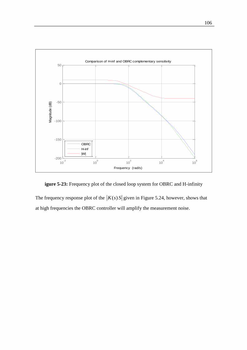
106
10-2
100
102
104
106
-200
-150
-100
-50
0
50
Magnitu
de (
dB
)
Comparison of H-inf and OBRC complementary sensitivity
Frequency (rad/s)
OBRC
H-inf
|W|
igure 5-23: Frequency plot of the closed loop system for OBRC and H-infinity
The frequency response plot of the ( )K s S given in Figure 5.24, however, shows that
at high frequencies the OBRC controller will amplify the measurement noise.
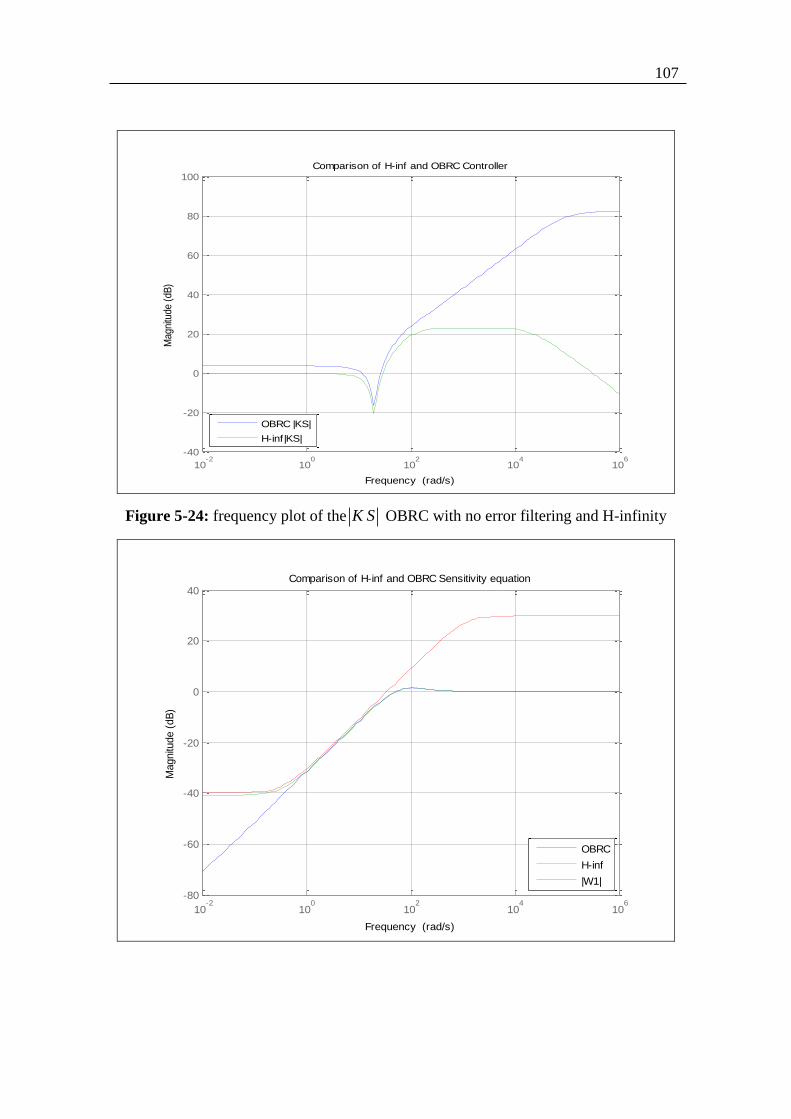
107
10-2
100
102
104
106
-40
-20
0
20
40
60
80
100M
agnitu
de (
dB
)
Comparison of H-inf and OBRC Controller
Frequency (rad/s)
OBRC |KS|
H-inf|KS|
Figure 5-24: frequency plot of the K S OBRC with no error filtering and H-infinity
10-2
100
102
104
106
-80
-60
-40
-20
0
20
40
Magnitu
de (
dB
)
Comparison of H-inf and OBRC Sensitivity equation
Frequency (rad/s)
OBRC
H-inf
|W1|
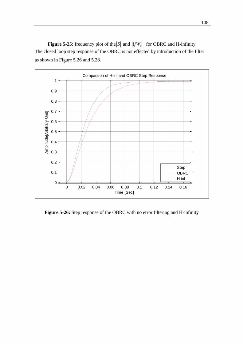
108
Figure 5-25: frequency plot of the 1 and 1S W for OBRC and H-infinity
The closed loop step response of the OBRC is not effected by introduction of the filter
as shown in Figure 5.26 and 5.28.
0 0.02 0.04 0.06 0.08 0.1 0.12 0.14 0.160
0.1
0.2
0.3
0.4
0.5
0.6
0.7
0.8
0.9
1
Comparison of H-inf and OBRC Step Response
Time [Sec]
Am
plit
ude[A
rbitra
ry U
nit]
Step
OBRC
H-inf
Figure 5-26: Step response of the OBRC with no error filtering and H-infinity
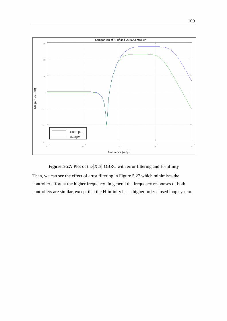
109
10
-2
10
0
10
2
10
4
10
6
-30
-20
-10
0
10
20
30
Ma
gn
itu
de
(d
B)
Comparison of H-inf and OBRC Controller
Frequency (rad/s)
OBRC |KS|
H-inf|KS|
Figure 5-27: Plot of the K S OBRC with error filtering and H-infinity
Then, we can see the effect of error filtering in Figure 5.27 which minimises the
controller effort at the higher frequency. In general the frequency responses of both
controllers are similar, except that the H-infinity has a higher order closed loop system.
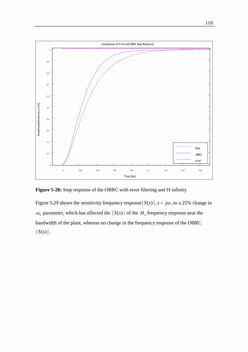
110
0 0.02 0.04 0.06 0.08 0.1 0.12 0.14 0.16
0
0.1
0.2
0.3
0.4
0.5
0.6
0.7
0.8
0.9
1
Comparison of H-inf and OBRC Step Response
Time [Sec]
Am
pli
tud
e[A
rbit
rary
Un
it]
Step
OBRC
H-inf
Figure 5-28: Step response of the OBRC with error filtering and H-infinity
Figure 5.29 shows the sensitivity frequency response | ( ) |S s , s j , to a 25% change in
n parameter, which has affected the | ( ) |S s of the Hfrequency response near the
bandwidth of the plant, whereas no change in the frequency response of the OBRC
| ( ) |S s .

111
Figure 5-29: Effects on S(s) when saturation is introduced at the Plant input
The change in n has been reflected in the | ( ) |S K s of both OBRC and Hcontrollers,
as shown in Figure 5.30. The change in n has been seen by the OBRC controller in the
higher frequency region, whereas the Hcontroller is effected in the lower frequency
region. Hence, it has reduced the robustness of the H controller.
Figure 5-30: Further effects on |KS(s)| when saturation is introduced at the plant input
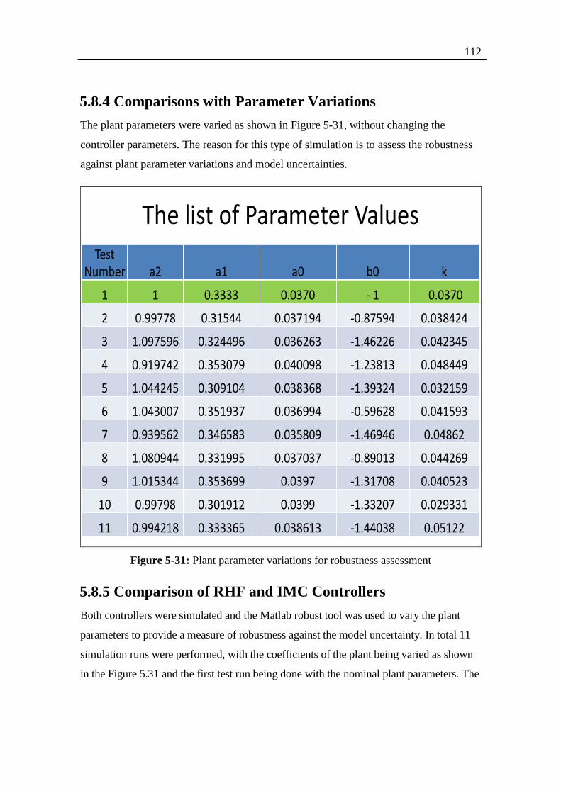
112
5.8.4 Comparisons with Parameter Variations
The plant parameters were varied as shown in Figure 5-31, without changing the
controller parameters. The reason for this type of simulation is to assess the robustness
against plant parameter variations and model uncertainties.
The list of Parameter ValuesTest
Number a2 a1 a0 b0 k
1 1 0.3333 0.0370 - 1 0.0370
2 0.99778 0.31544 0.037194 -0.87594 0.038424
3 1.097596 0.324496 0.036263 -1.46226 0.042345
4 0.919742 0.353079 0.040098 -1.23813 0.048449
5 1.044245 0.309104 0.038368 -1.39324 0.032159
6 1.043007 0.351937 0.036994 -0.59628 0.041593
7 0.939562 0.346583 0.035809 -1.46946 0.04862
8 1.080944 0.331995 0.037037 -0.89013 0.044269
9 1.015344 0.353699 0.0397 -1.31708 0.040523
10 0.99798 0.301912 0.0399 -1.33207 0.029331
11 0.994218 0.333365 0.038613 -1.44038 0.05122
Figure 5-31: Plant parameter variations for robustness assessment
5.8.5 Comparison of RHF and IMC Controllers
Both controllers were simulated and the Matlab robust tool was used to vary the plant
parameters to provide a measure of robustness against the model uncertainty. In total 11
simulation runs were performed, with the coefficients of the plant being varied as shown
in the Figure 5.31 and the first test run being done with the nominal plant parameters. The
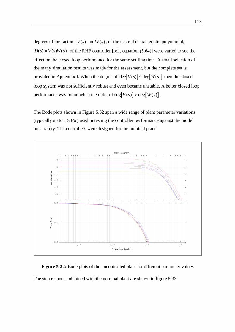
113
degrees of the factors, ( )V s and ( )W s , of the desired characteristic polynomial,
( ) ( ) ( )D s V s W s , of the RHF controller [ref., equation (5.64)] were varied to see the
effect on the closed loop performance for the same settling time. A small selection of
the many simulation results was made for the assessment, but the complete set is
provided in Appendix I. When the degree of deg ( ) deg ( )V s W s then the closed
loop system was not sufficiently robust and even became unstable. A better closed loop
performance was found when the order of deg ( ) deg ( )V s W s .
The Bode plots shown in Figure 5.32 span a wide range of plant parameter variations
(typically up to 30% ) used in testing the controller performance against the model
uncertainty. The controllers were designed for the nominal plant.
-20
-15
-10
-5
0
5
Magnitu
de (
dB
)
10-3
10-2
10-1
100
120
150
180
Phase (
deg)
Bode Diagram
Frequency (rad/s)
Figure 5-32: Bode plots of the uncontrolled plant for different parameter values
The step response obtained with the nominal plant are shown in figure 5.33.

114
Figure 5-33: Step responses for the plant precisely matching the nominal plant model
Both control methods were subjected to the same plant mismatches and the results of
the simulations are shown in Figures 5.34 and 5.35. It can be seen that the nominal
performance of both controllers (IMC and RHF) is satisfactory and their closed loop
response to a step input remains stable. The only significant difference that can be seen
is at the start of the step response where the pre-compensator is minimising the effect of
the zero’s as shown in Figure 5.36 and they have different settling times. The response
time of the RHF-controller is delayed because of the reference input signal being
filtered. Clearly the RHF-controller. The IMC controller has stable control on the plant
as shown in Figure 5.34 but the deviation against model uncertainty is considerable with
large overshoots with extreme plant mismatches, in contrast to the RHF controller,
which maintains the specified transient response specification very tightly with only a
very small deviation from the nominal performance, as shown in Figure 5-35.

115
0 5 10 15 20 25 30 35 40 45 50-0.2
0
0.2
0.4
0.6
0.8
1
1.2
Time [s]
proc
ess
out
y [t
]Polynomial Control Min Order with pre-comp + Integral Action Ts=10s Tso=1s n=5 m=1
Figure 5-34: Step response of RHF with model uncertainty
0 5 10 15 20 25 30 35 40 45 50-0.2
0
0.2
0.4
0.6
0.8
1
1.2
1.4
Time [s]
pro
cess o
ut
y [
t]
Internal Model Control
Figure 5-35: Step response of IMC with model uncertainty
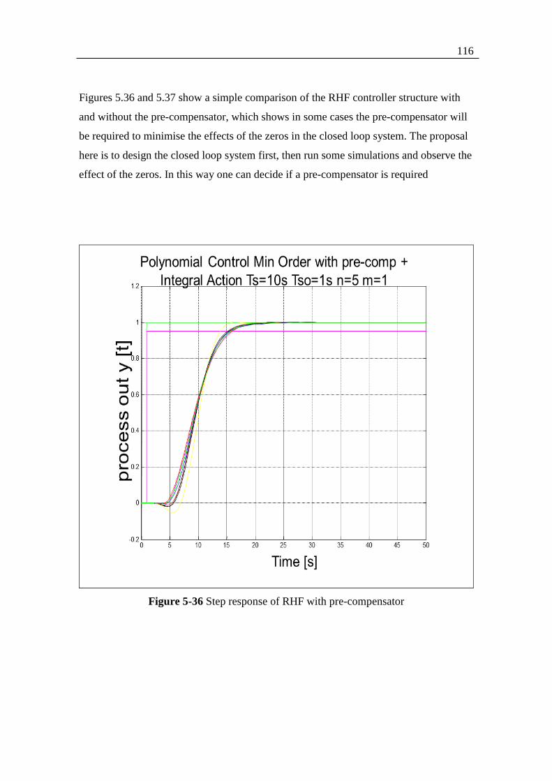
116
Figures 5.36 and 5.37 show a simple comparison of the RHF controller structure with
and without the pre-compensator, which shows in some cases the pre-compensator will
be required to minimise the effects of the zeros in the closed loop system. The proposal
here is to design the closed loop system first, then run some simulations and observe the
effect of the zeros. In this way one can decide if a pre-compensator is required
Figure 5-36 Step response of RHF with pre-compensator
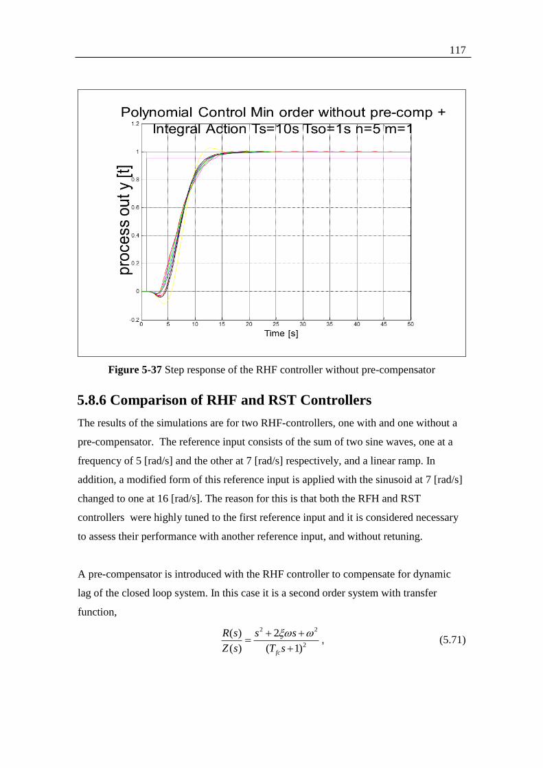
117
Figure 5-37 Step response of the RHF controller without pre-compensator
5.8.6 Comparison of RHF and RST Controllers
The results of the simulations are for two RHF-controllers, one with and one without a
pre-compensator. The reference input consists of the sum of two sine waves, one at a
frequency of 5 [rad/s] and the other at 7 [rad/s] respectively, and a linear ramp. In
addition, a modified form of this reference input is applied with the sinusoid at 7 [rad/s]
changed to one at 16 [rad/s]. The reason for this is that both the RFH and RST
controllers were highly tuned to the first reference input and it is considered necessary
to assess their performance with another reference input, and without retuning.
A pre-compensator is introduced with the RHF controller to compensate for dynamic
lag of the closed loop system. In this case it is a second order system with transfer
function,
2 2
2
( ) 2
( ) ( 1)fc
R s s s
Z s T s
, (5.71)

118
where 0.53 and 10 . The second order low pass filter element is included to
enable straightforward implementation as a dynamical system, instead of software
differentiation, such as in a dSPACE system using Simulink. Normally, the polynomial,
2 22s s , would be the same as the nominal characteristic polynomial of the
closed loop system. The filter, however, would introduce a certain amount of dynamic
lag, determined by the time constant, fcT , but since this is outside the feedback loop it
would not cause oscillations or destabilise the closed loop system.
For some applications, the ideal way of compensating for the dynamic lag of a closed
loop system is pre-computation of the first and second derivatives of the reference input
and feeding these forward together with the reference input with relative weightings of
2 and2 , respectively. This would avoid the need for a low pass filter.
Figure 5.38 shows that the pre-compensator has minimised the error and compensates
for the dynamic lag.
Figure 5-38: RFH with pre-compensator response to reference input
(sine(7t)+sine(5t)+ramp)
Figure 5.39 shows the dynamic lag occurring without the pre-compensator.
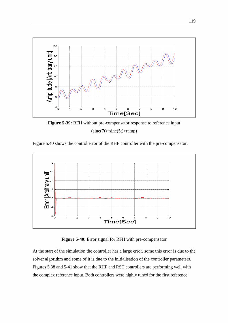
119
Figure 5-39: RFH without pre-compensator response to reference input
(sine(7t)+sine(5t)+ramp)
Figure 5.40 shows the control error of the RHF controller with the pre-compensator.
Figure 5-40: Error signal for RFH with pre-compensator
At the start of the simulation the controller has a large error, some this error is due to the
solver algorithm and some of it is due to the initialisation of the controller parameters.
Figures 5.38 and 5-41 show that the RHF and RST controllers are performing well with
the complex reference input. Both controllers were highly tuned for the first reference
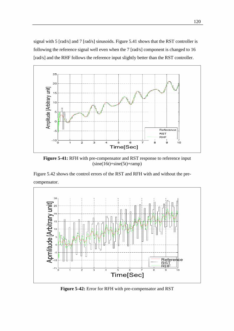
120
signal with 5 [rad/s] and 7 [rad/s] sinusoids. Figure 5.41 shows that the RST controller is
following the reference signal well even when the 7 [rad/s] component is changed to 16
[rad/s] and the RHF follows the reference input slightly better than the RST controller.
Figure 5-41: RFH with pre-compensator and RST response to reference input
(sine(16t)+sine(5t)+ramp)
Figure 5.42 shows the control errors of the RST and RFH with and without the pre-
compensator.
Figure 5-42: Error for RFH with pre-compensator and RST

121
The RHF controller effort, however, is much higher than that of the RST controller as
shown in Figure 5.43, which is the price to pay for the smaller error.
Figure 5-43: Plot of controller effort for RFH with pre-compensator and RST
5.8.7 Summary
Both controllers provide a robust solution for a given plant and the question is the degree
of robustness which will depend on the quality of the linearised model and how close is
the nominal model to the mean of the plant. Both controllers provide the designer with an
adequate degree of adjustability and flexibility. Also the RHF design process is a simple
as that of the IMC. This could also be said of the RST with similar approach to the RHF.
H-infinity, however, and RST (at present) are using a sophisticated mathematical
optimisation which will require a complex design procedure and high computation power.
The degree of robustness which the controller can yield depends on the linearised model
and the closed loop specification. As soon as an un-modelled element is introduced in the
plant, the H-infinity controller must be redesigned based on new constraints, which is an
expensive and time consuming process. In comparison, the OBRC, RHF, and IMC can be
re tuned to certain degree. Also all of the design methods which are compared in this
work provide robustness, but some are more time consuming and costlier than others.

122
6. Comparison of Control Techniques for Engine Application
6.1 Overview
In this chapter the IMC controller and OBRC controller performances are compared for
the Diesel engine application. This comparison is basically by simulation but some
experimental results are also presented for the OBRC controller.
6.2 The OBRC Controller
6.2.1 Overall Structure
Figure 6-1 shows the overall block diagram of the observer based control system for
speed control of the Diesel engine including the external load torque.
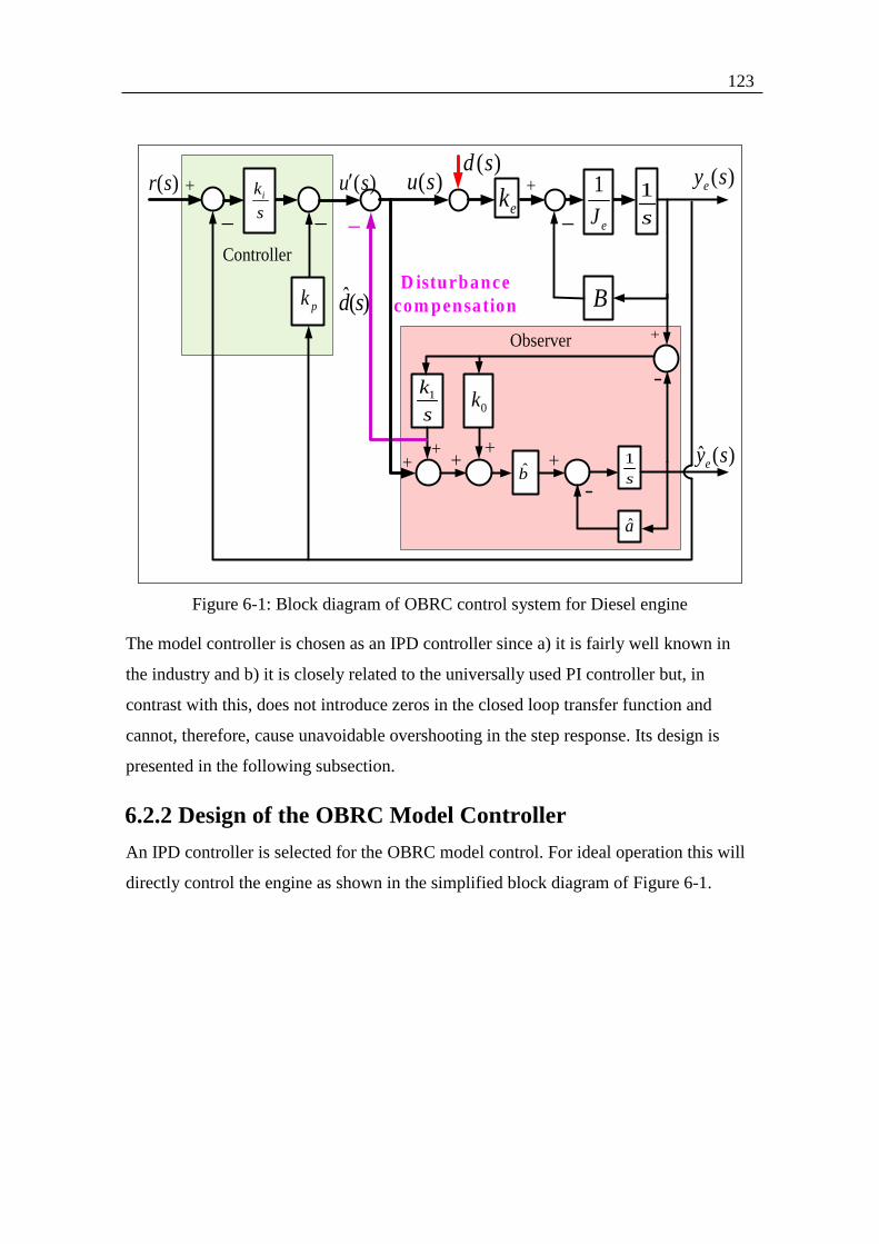
123
Controller
Observer
ik
s
1k
s
1
s
0k
a
b
1
s
pk
( )r sek
1
eJ
D isturbance
com pensation
( )ey s
ˆ ( )ey s
B
( )u s( )u s
ˆ( )d s
( )d s
Figure 6-1: Block diagram of OBRC control system for Diesel engine
The model controller is chosen as an IPD controller since a) it is fairly well known in
the industry and b) it is closely related to the universally used PI controller but, in
contrast with this, does not introduce zeros in the closed loop transfer function and
cannot, therefore, cause unavoidable overshooting in the step response. Its design is
presented in the following subsection.
6.2.2 Design of the OBRC Model Controller
An IPD controller is selected for the OBRC model control. For ideal operation this will
directly control the engine as shown in the simplified block diagram of Figure 6-1.
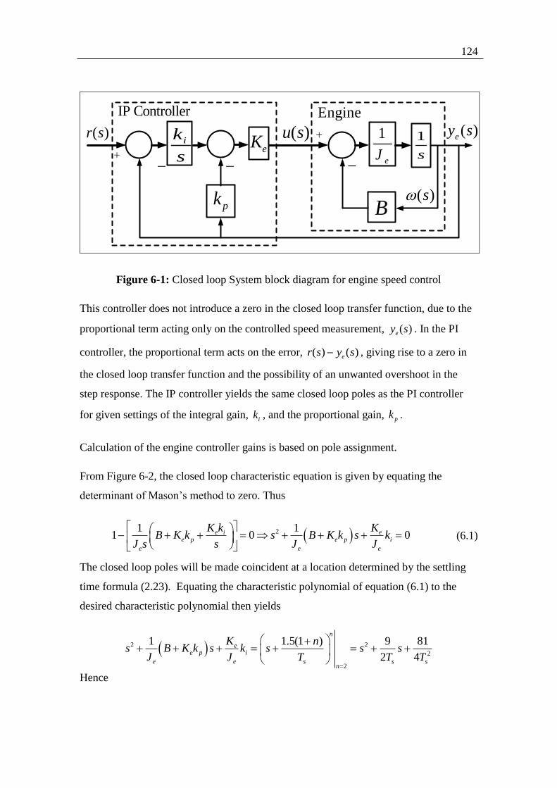
124
1
s
ik
s
( )ey s( )r s
pkB
eK1
eJ
( )u s
( )s
IP Controller Engine
Figure 6-1: Closed loop System block diagram for engine speed control
This controller does not introduce a zero in the closed loop transfer function, due to the
proportional term acting only on the controlled speed measurement, ( )ey s . In the PI
controller, the proportional term acts on the error, ( ) ( )er s y s , giving rise to a zero in
the closed loop transfer function and the possibility of an unwanted overshoot in the
step response. The IP controller yields the same closed loop poles as the PI controller
for given settings of the integral gain, ik , and the proportional gain, pk .
Calculation of the engine controller gains is based on pole assignment.
From Figure 6-2, the closed loop characteristic equation is given by equating the
determinant of Mason’s method to zero. Thus
21 11 0 0e i e
e p e p i
e e e
K k KB K k s B K k s k
J s s J J
(6.1)
The closed loop poles will be made coincident at a location determined by the settling
time formula (2.23). Equating the characteristic polynomial of equation (6.1) to the
desired characteristic polynomial then yields
2 2
2
2
1 1.5(1 ) 9 81
2 4
n
ee p i
e e s s sn
K ns B K k s k s s s
J J T T T
Hence
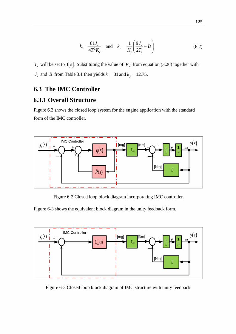
125
2
81 1 9and
4 2
e ei p
s e e s
J Jk k B
T K K T
(6.2)
sT will be set to 1 s . Substituting the value of eK from equation (3.26) together with
eJ and B from Table 3.1 then yields 81and 12.75i pk k .
6.3 The IMC Controller
6.3.1 Overall Structure
Figure 6.2 shows the closed loop system for the engine application with the standard
form of the IMC controller.
[Nm]
[mg] [Nm]
gainE1
ej
1
s
rf
( )q s
ˆ( )P s
( )ry s ( )y sIMC Controller
Figure 6-2 Closed loop block diagram incorporating IMC controller.
Figure 6-3 shows the equivalent block diagram in the unity feedback form.
[Nm]
[mg] [Nm]
gainE1
ej
1
s
rf
( )ry s ( )y s( )imcC s
IMC Controller
Figure 6-3 Closed loop block diagram of IMC structure with unity feedback
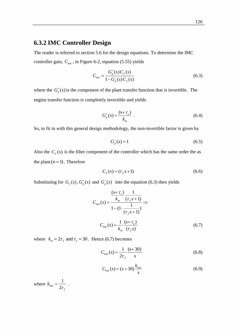
126
6.3.2 IMC Controller Design
The reader is referred to section 5.6 for the design equations. To determine the IMC
controller gain, imcC , in Figure 6-2, equation (5.55) yields
( ) ( )
1 ( ) ( )
p f
imc
p f
G s C sC
G s C s
(6.3)
where the ( )pG sis the component of the plant transfer function that is invertible. The
engine transfer function is completely invertible and yields
(s )
( ) ep
m
G sk
. (6.4)
So, to fit in with this general design methodology, the non-invertible factor is given by
( ) 1pG s (6.5)
Also the ( )fC s is the filter component of the controller which has the same order the as
the plant ( 1)n . Therefore
( ) ( 1)f fC s s (6.6)
Substituting for ( )fG s , ( )pG s and ( )pG s
into the equation (6.3) then yields
(s ) 1
( 1)( )
11 (1 )
( 1)
e
m f
imc
f
k sC s
s
(s )1
( )( )
eimc
m f
C sk s
(6.7)
where 2 and 30m f ek . Hence (6.7) becomes
1 (s 30)
( )2
imc
f
C ss
(6.8)
( ) ( 30) imcimc
kC s s
s (6.9)
where 1
2imc
f
k
.
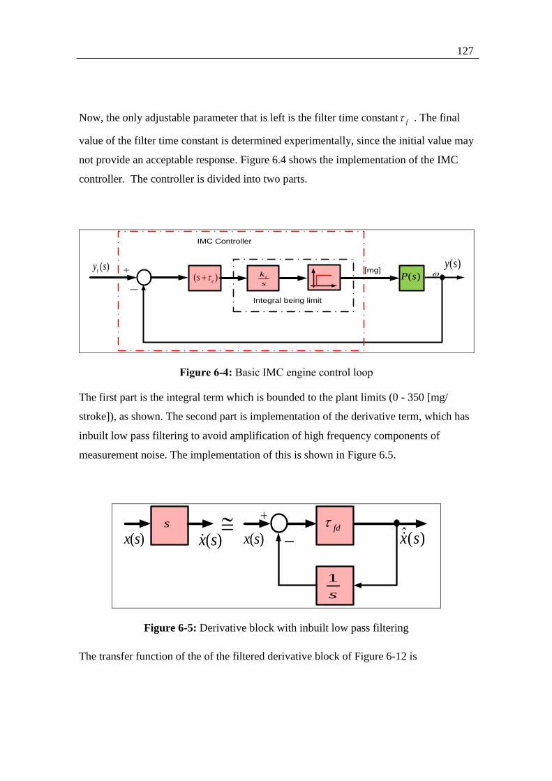
127
Now, the only adjustable parameter that is left is the filter time constantf . The final
value of the filter time constant is determined experimentally, since the initial value may
not provide an acceptable response. Figure 6.4 shows the implementation of the IMC
controller. The controller is divided into two parts.
[mg]
( )ry s ( )y s
IMC Controller
( )es ( )P sik
s
Integral being limit
Figure 6-4: Basic IMC engine control loop
The first part is the integral term which is bounded to the plant limits (0 - 350 [mg/
stroke]), as shown. The second part is implementation of the derivative term, which has
inbuilt low pass filtering to avoid amplification of high frequency components of
measurement noise. The implementation of this is shown in Figure 6.5.
1
s
fds
( )x s ( )x s ( )x s ˆ( )x s
Figure 6-5: Derivative block with inbuilt low pass filtering
The transfer function of the of the filtered derivative block of Figure 6-12 is
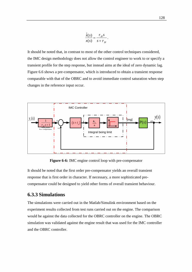
128
ˆ( )
( )
fd
fd
sx s
x s s
.
It should be noted that, in contrast to most of the other control techniques considered,
the IMC design methodology does not allow the control engineer to work to or specify a
transient profile for the step response, but instead aims at the ideal of zero dynamic lag.
Figure 6.6 shows a pre-compensator, which is introduced to obtain a transient response
comparable with that of the OBRC and to avoid immediate control saturation when step
changes in the reference input occur.
[mg]
( )ry s ( )y s
IMC Controller
( )es ( )P sik
s
Integral being limitPr
1
1pf
e compensator
s
Figure 6-6: IMC engine control loop with pre-compensator
It should be noted that the first order pre-compensator yields an overall transient
response that is first order in character. If necessary, a more sophisticated pre-
compensator could be designed to yield other forms of overall transient behaviour.
6.3.3 Simulations
The simulations were carried out in the Matlab/Simulink environment based on the
experiment results collected from test runs carried out on the engine. The comparison
would be against the data collected for the OBRC controller on the engine. The OBRC
simulation was validated against the engine result that was used for the IMC controller
and the OBRC controller.
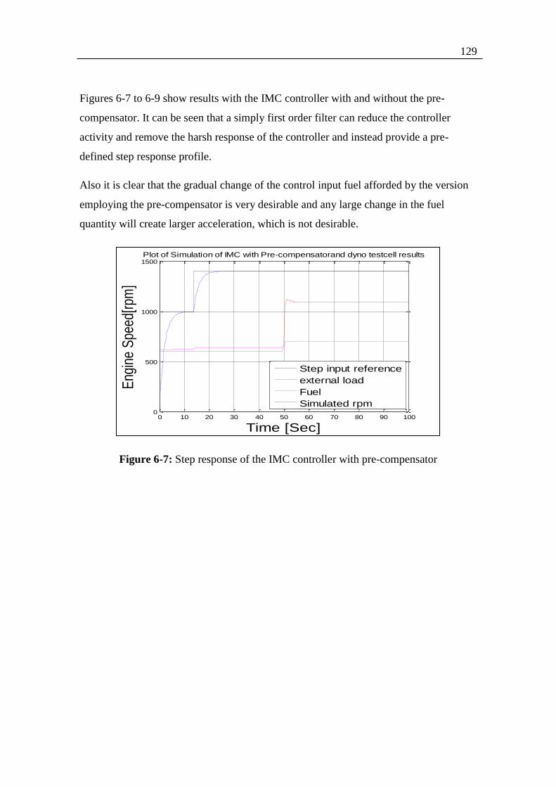
129
Figures 6-7 to 6-9 show results with the IMC controller with and without the pre-
compensator. It can be seen that a simply first order filter can reduce the controller
activity and remove the harsh response of the controller and instead provide a pre-
defined step response profile.
Also it is clear that the gradual change of the control input fuel afforded by the version
employing the pre-compensator is very desirable and any large change in the fuel
quantity will create larger acceleration, which is not desirable.
Figure 6-7: Step response of the IMC controller with pre-compensator
0 10 20 30 40 50 60 70 80 90 1000
500
1000
1500Plot of Simulation of IMC with Pre-compensatorand dyno testcell results
Time [Sec]
Eng
ine
Spe
ed[r
pm]
Step input reference
external load
Fuel
Simulated rpm
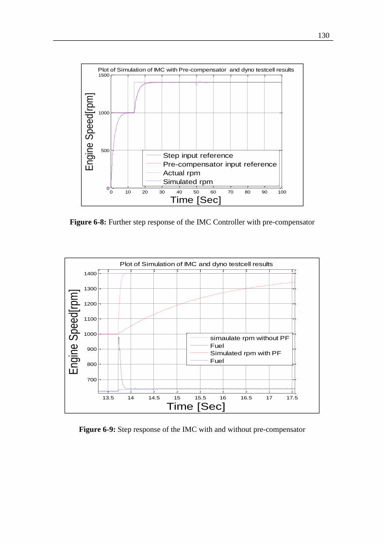
130
Figure 6-8: Further step response of the IMC Controller with pre-compensator
Figure 6-9: Step response of the IMC with and without pre-compensator
0 10 20 30 40 50 60 70 80 90 1000
500
1000
1500Plot of Simulation of IMC with Pre-compensator and dyno testcell results
Time [Sec]
Engin
e S
peed[r
pm
]
Step input reference
Pre-compensator input reference
Actual rpm
Simulated rpm
13.5 14 14.5 15 15.5 16 16.5 17 17.5
700
800
900
1000
1100
1200
1300
1400
Plot of Simulation of IMC and dyno testcell results
Time [Sec]
Eng
ine
Spe
ed[r
pm]
simaulate rpm without PF
Fuel
Simulated rpm with PF
Fuel
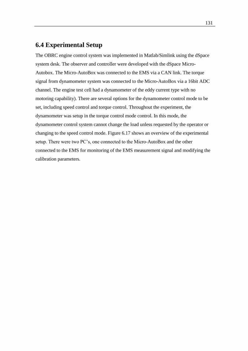
131
6.4 Experimental Setup
The OBRC engine control system was implemented in Matlab/Simlink using the dSpace
system desk. The observer and controller were developed with the dSpace Micro-
Autobox. The Micro-AutoBox was connected to the EMS via a CAN link. The torque
signal from dynamometer system was connected to the Micro-AutoBox via a 16bit ADC
channel. The engine test cell had a dynamometer of the eddy current type with no
motoring capability). There are several options for the dynamometer control mode to be
set, including speed control and torque control. Throughout the experiment, the
dynamometer was setup in the torque control mode control. In this mode, the
dynamometer control system cannot change the load unless requested by the operator or
changing to the speed control mode. Figure 6.17 shows an overview of the experimental
setup. There were two PC’s, one connected to the Micro-AutoBox and the other
connected to the EMS for monitoring of the EMS measurement signal and modifying the
calibration parameters.

132
Control desk and Monitoring ECU
Parameters
Engine Management
System
dSPACE sytem MicroAutoBox(14001/
1505 PowerPc800Mhz+burst
sample acquistion board
DriveShaftDyno.
Engine Test Cell
CAN Link at 250 Kb for Bypass
Ethern
et
CAN Link At 250 Kb for ECU Measurement and Calibration
Link To Test Cell
hsrn
ess
Figure 6-10 Experiment Setup
6.5 Comparison of Simulation Results and Test Results
The data collected from the test cell was replayed in the Matlab environment. The
simulation was run under the same conditions as the test cell with the demanded engine
speed as a common input. After each simulation run, the results were compared with the
corresponding data collected from the test cell. In Figure 6-11, the physical system and
the simulation commence with the control system operating in the steady state with a
reference speed input of 500 rpm and zero load torque. A step increase of the
reference speed input to 1000 rpm is applied at 0 st . This is followed by a further
step increase in the reference speed to 1400 rpm at 14 st . This reference input is
maintained thereafter but a step load torque of 500 Nm is applied at 50 st . It can
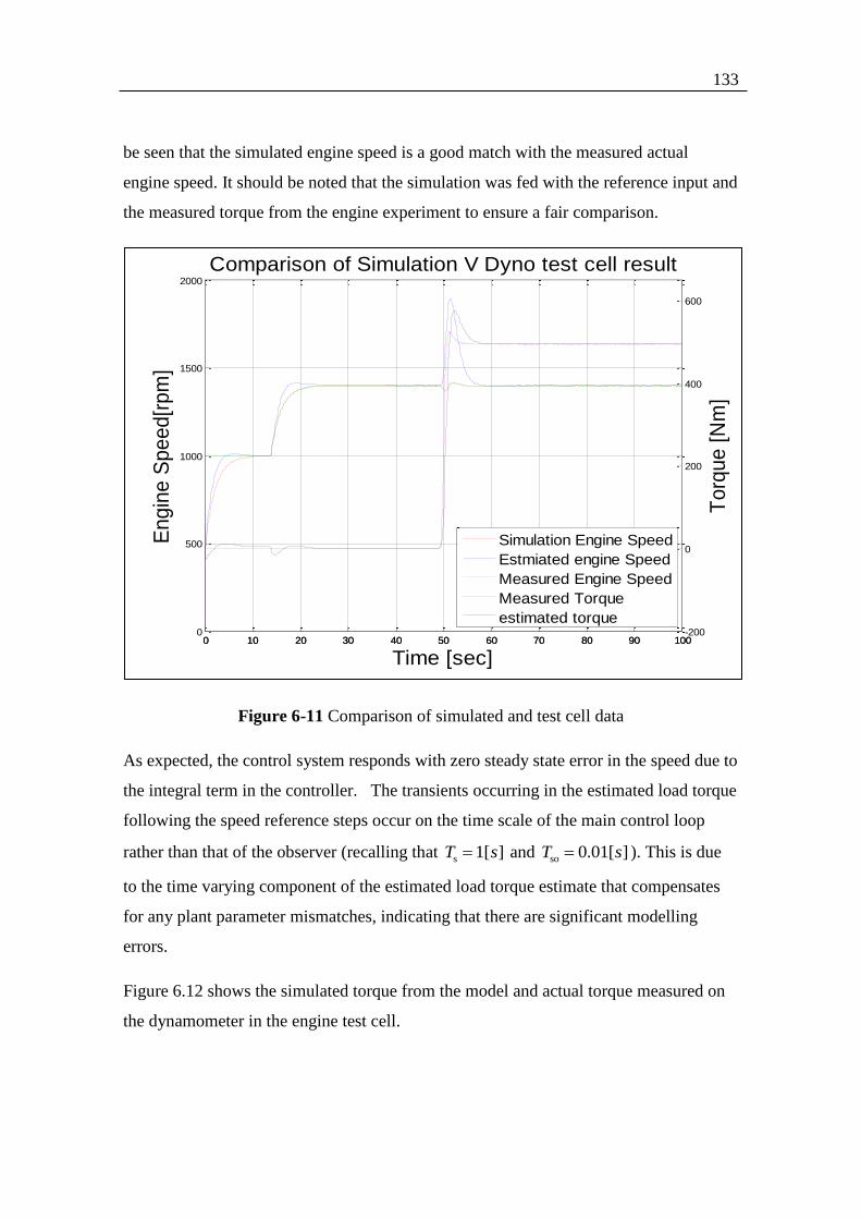
133
be seen that the simulated engine speed is a good match with the measured actual
engine speed. It should be noted that the simulation was fed with the reference input and
the measured torque from the engine experiment to ensure a fair comparison.
Figure 6-11 Comparison of simulated and test cell data
As expected, the control system responds with zero steady state error in the speed due to
the integral term in the controller. The transients occurring in the estimated load torque
following the speed reference steps occur on the time scale of the main control loop
rather than that of the observer (recalling that s 1[ ]T s and so 0.01[ ]T s ). This is due
to the time varying component of the estimated load torque estimate that compensates
for any plant parameter mismatches, indicating that there are significant modelling
errors.
Figure 6.12 shows the simulated torque from the model and actual torque measured on
the dynamometer in the engine test cell.
0 10 20 30 40 50 60 70 80 90 1000
500
1000
1500
2000
Engin
e S
peed[r
pm
]
Comparison of Simulation V Dyno test cell result
Time [sec]
0 10 20 30 40 50 60 70 80 90 100-200
0
200
400
600
Torq
ue [
Nm
]
Simulation Engine Speed
Estmiated engine Speed
Measured Engine Speed
Measured Torque
estimated torque
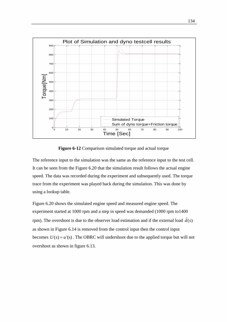
134
Figure 6-12 Comparison simulated torque and actual torque
The reference input to the simulation was the same as the reference input to the test cell.
It can be seen from the Figure 6.20 that the simulation result follows the actual engine
speed. The data was recorded during the experiment and subsequently used. The torque
trace from the experiment was played back during the simulation. This was done by
using a lookup table.
Figure 6.20 shows the simulated engine speed and measured engine speed. The
experiment started at 1000 rpm and a step in speed was demanded (1000 rpm to1400
rpm). The overshoot is due to the observer load estimation and if the external load ˆ( )d s
as shown in Figure 6.14 is removed from the control input then the control input
becomes ( ) '(s)U s u . The OBRC will undershoot due to the applied torque but will not
overshoot as shown in figure 6.13.
0 10 20 30 40 50 60 70 80 90 1000
100
200
300
400
500
600
700
800
900
Plot of Simulation and dyno testcell results
Time [Sec]
Tor
que[
Nm
]
Simulated Torque
Sum of dyno torque+Friction torque

135
Figure 6-13 Comparison of actual engine speed with simulated engine speed
Figure 6-14 Comparison of the torque and estimated
0 10 20 30 40 50 60 70 80 90 1000
200
400
600
800
1000
1200
1400
1600
1800
2000
Plot of Simulation and dyno testcell results
Time [Sec]
En
gin
e S
pe
ed
[rp
m]
Input reference
Simulated engine speed
Estimated engine speed
Actual engine speed
0 10 20 30 40 50 60 70 80 90 100-100
0
100
200
300
400
500
600
Plot of Simulation and dyno testcell results
Time [Sec]
Torq
ue[N
m]
Simulated Torque
Actual dyno torque
136
Finally, to demonstrate that the feedback of the load torque estimate in OBRC is the key
to its robustness, Figure 6-15 shows two responses of the control system with a constant
reference input speed and a step external load torque applied at 49.5[s]t . It is evident
that this feedback reduces the magnitude of the transient speed error by an order of
magnitude.
49 49.5 50 50.5 51 51.5 52
1395
1396
1397
1398
1399
1400
Plot of OBRC Speed Control With and without Externalload
Time [Sec]
Engi
ne
Sp
ee
d[r
pm
]
( ) '(s)U s u
ˆ( ) '(s) d(s)U s u
Figure 6-15: Plot of OBRC with and without external load signal
137
7. Conclusions and Recommendations for Further
Research
7.1 Conclusions
7.1.1 OBRC
The OBRC methodology works very well for the class of plants excluding zeros in the
right half plane and pure time delays. The inverse dynamic modeling technique allows a
relatively complex plant to be modeled as two subsystems, a simple one in the forward
path and one that is more difficult to model accurately, which is situated in the feedback
path to the plant input. The effects of this feedback path subsystem are then represented
by an equivalent disturbance input that can be estimated in an observer, using just an
integrator, together with the state of the simple forward path subsystem. This work
revealed a useful potential application in which the observer is used as a disturbance
estimator to gain useful information, such as the load mass carried by a vehicle. Without
this aid, the load torque would have to be measured by highly expensive torque
transducers or complex modeling of the vehicle system. The main issue with OBRC is
that it effectively cancels any zeros with closed loop poles automatically and therefore
creates unstable closed loop modes if any of the zeros lie in the right half of the s-plane.
Analysis of the OBRC during its development for plants of order greater than two,
especially those with zeros, entailed very labor intensive derivations of the complete
system characteristic polynomial for gain determination. As a result of this, a computer
aided method was developed to determine the gains of any linear system for pole
placement in which the relationship between the gains and the coefficients of the
characteristic polynomial is linear, as shown in the Appendix. The Dodds settling time
formula was used for the observer design and the model state controller design for the
OBRC controllers. In the process of doing so, it was realised that this is a useful tool for
any linear system that can be designed by pole placement.
138
7.1.2 Comparison of OBRC with Other Control Techniques
H-infinity controller
The basic OBRC controller was compared with an H-infinity controller, and the results
were much the same for linear operation without control saturation. The difference was
that the OBRC controller would produce more control activities at high frequencies.
This is considered to be undesirable, from a practical aspect of the plant (actuator
chattering and wear over the life the actuator). In view of this, a modified a low pass
filter was introduced in the OBRC structure. The low pass filter limits the controller
effort at high frequency and brings the frequency response of the ( )k s S for the OBRC
into line with the H-infinity controller, and the results were still comparable. The OBRC
controller, however, was able to cope with control saturation while the H-infinity
controller was unable to do so.
Polynomial Controller, RST and IMC Controller
The RHF-controller has identical structure to the RST-controller. However, the two
differ in the documented design approaches as a result of their independent evolvement,
and also the fact that the RHF and RST controllers are formulated, respectively, in the
continuous Laplace and discrete z domains. The RHF-Controller comes with a simple
design methodology for full pole placement. An academic example was used to
compare the RHF and IMC controllers. A parametric study was carried out and the
result of the simulation and frequency analysis showed that the RHF-controller is more
robust to model uncertainty than the IMC controller, with the model parameters
mismatched relative to the plant parameters by up to 30% for 10 simulation runs. The
plant of the second academic example incorporated a pure time delay. The RHF-
Controller provided good simulation results for a perfectly matched plant model but the
degree robustness was reduced to a marginal point. In this case a pre-compensator had
to develop to minimise the phase lag of the plant. Also it was shown when the reference
input was changed significantly from 7 rad/s to 14 rad/s then both controllers start to
lose tracking of the reference signal. Also, the RST controller was less robust than the
RHF-controller.
139
7.1.3 Engine Test
The experimental test results showed that the robust controllers allow the possibility of
eliminating the tuning process, but dependent on the accuracy of the available plant
model. In the case of the diesel engine speed control, the model is very simple and no
major issue is experienced in getting the design right first time. During these tests,
nonlinearities were inserted into the plant model of the OBRC observer and the
controller, but this did not require redesign of the controller or the observer correction
loop gains for the OBRC. The torque estimation from the observer was compared with
measurements from a torque transducer revealing an error of less than 2% over a large
range of torques (0 to 1400 Nm). The OBRC was the only controller employed in these
tests because the other control techniques did not provide any means of estimating the
external load torque.
7.2 Overall Assessment
The simulation results, engine experimental work and theoretical investigations
combine to confirm that generally more than one approach to solve a control problem
may be successful. Some methods, of course, can handle plants better than others. The
RHF, OBRC and H-infinity controllers proved to be the most robust, but with the
reservation that the H-infinity controller could not handle control saturation. The IMC
stands alone in that it can handle pure time delays in the plant. In terms of engineering
cost and effort with modern software packages, as influenced by simplicity of the
design process and accessibility to many industrial users, one would rank the RHF, IMC
and OBRC-controllers more or less equally. In contrast, the RST and H-infinity
controller design processes are complex and require sophisticated software tools and
staff with a strong mathematical background to undertake in-depth development work.
Although it is not essential to apply these associated computer aided design tools,
however, dealing with issues arising in a particular control system development
programme would be difficult without them.

140
7.3 Recommendations for Further Research
The research programme has revealed the following further investigations
1. To investigate the possibility of translating the z-domain based RST design
methodologies to the Laplace domain for direct use with the RHF controller, and
the identification of any advantages over the simple pole placement.
2. The development of a discrete version of the RHF controller that should be
applicable to plants containing pure time delays
3. The design of reference input generators that enable derivative feed-forward for
dynamic lag compensation to be carried out without the need for higher order
software differentiation
4. Modification of the OBRC structure to enable plants with zeros in the right half
of the s-plane to be controlled without the creation of unstable closed loop
modes due to the zero cancellation inherent in the present structure. This alone
would yield overshoots and/or undershoots of the step response in certain cases,
requiring the design of pre-compensators outside the feedback loop using special
pole placement techniques such as zero mirroring [19].
141
APPENDIX
A.1 Sensitivity Function
This section will define the sensitivity function for a given closed loop transfer function.
Let us consider a non-dynamic system with a unity feedback structure having a forward
path gain of 1G and feedback gain, 2G . The loop gain is 1 2G G and, if we assume
negative feedback, the closed loop gain is given by
1
1 21
GT
G G
(A.1)
In the real plant the parameter 1G may vary throughout the plant life due to wear and
operating conditions. The change in 1G is denoted by 1G and the relative change is
given by 11
G
G
. The corresponding change in the T is T and the relative change is given
byT
T
.
The sensitivity function 1
T
GS is defined as
1
1
11 1
1
1
11
lim lim0 0
T
G
TTGT
G T
GG
T GS
G TG G
(A.2)
To obtain the expression for the sensitivity function we need to determine 1
T
G
from the
closed loop transfer function A.1. To differentiate the closed loop transfer function we
need to use the quotient rule which is given by
1 1
2
1 1
u vv u
T u G G
G G v v
(A.3)
where 1u G and 1 21v G G . Then equation (A.3) becomes
1 2 1 2
2 2
1 1 2 1 2
1 .1 1
1 1
G G G GT
G G G G G
(A.4)

142
Then substituting for 1
T
G
and T in equation (A.2) using, respectively, equations (A.4)
and (A.1) yields
1
1
21 1 21 2
1 2
1 1
111
T
G
GS
G G GG GG G
(A.5)
The sensitivity equation (A.5) shows that the sensitivity function can be made as small
as we desire by increasing the return difference 1 2(1 )G G .
The foregoing sensitivity theory may be applied to linear dynamic systems simply by
replacing the constants, 1G and 2G , by transfer functions, 1( )G s and 2( )G s . Then the
sensitivity function (A5) becomes
1
1 2
1( )
1 ( ) ( )
T
GS sG s G s
(A.6)
The associate transfer function,
1
1 2
1 2
( ) ( )( )
1 ( ) ( )
T
G
G s G sR s
G s G s
(A.7)
is referred to as the complementary sensitivity function since
1 1( ) ( ) 1T T
G GS s R s (A.8)
Note that viewed in the frequency domain, the effect of the feedback control system in
reducing the sensitivity is achieved for those frequencies where 1 2|1 ( ) ( ) |G j G j is
large.

143
A.2Computer Aided Pole Assignment
A.2.1 Background Instability has been experienced when attempting OBRC for some plants, despite the
observer correction loop being stable when isolated from the rest of the system. Since
the plant model in the observer is mismatched with respect to the real plant and the
gains of the correction loop cannot be infinite, insertion of the observer in the system
will shift the poles of its model correction loop and the poles of the model state
feedback control loop will not be in the originally planned locations. The instability is
attributed to this process. It was therefore decided to attempt design of the OBRC
system by pole placement using the combined sets of observer and state feedback gains.
This, however, proved to be very time consuming due to the complex block diagram
algebra if the order of the plant exceeds two and even becomes near impossible in some
cases. This provided the motivation to develop a numerical method for such pole
assignment and a Matlab script for its automation. Two schemes were investigated
initially, one in which the coefficients of the characteristic equation have to be linear
with respect to the gains and the other free of this restriction in order to cater for
products of the observer and state feedback gains that appear in the characteristic
equation coefficients of the complete OBRC system. The restricted version, has proven
to be successful and this presented in the following sections. The need for a computer
implemented tool was originated by the author. The solution was produced by S J
Dodds and the author prepared the MATLAB code listed in section A2.4. Further
research is necessary to derive an unrestricted version.
A2.2 Linear Characteristic Polynomial Interpolation
In many linear systems that can be designed by pole assignment, the characteristic
polynomial
1
1 1 0( ) ( ) ( )n n
ns a s a s a
k k k
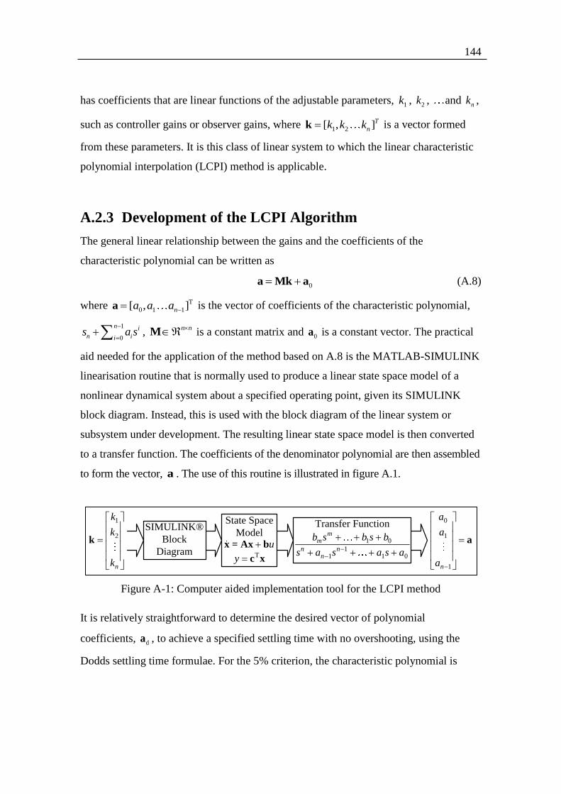
144
has coefficients that are linear functions of the adjustable parameters, 1k ,
2k , and nk ,
such as controller gains or observer gains, where 1 2[ , ]T
nk k kk is a vector formed
from these parameters. It is this class of linear system to which the linear characteristic
polynomial interpolation (LCPI) method is applicable.
A.2.3 Development of the LCPI Algorithm
The general linear relationship between the gains and the coefficients of the
characteristic polynomial can be written as
0 a Mk a (A.8)
where T
0 1 1[ , ]na a a a is the vector of coefficients of the characteristic polynomial,
1
0
n i
n iis a s
,
n nM is a constant matrix and 0a is a constant vector. The practical
aid needed for the application of the method based on A.8 is the MATLAB-SIMULINK
linearisation routine that is normally used to produce a linear state space model of a
nonlinear dynamical system about a specified operating point, given its SIMULINK
block diagram. Instead, this is used with the block diagram of the linear system or
subsystem under development. The resulting linear state space model is then converted
to a transfer function. The coefficients of the denominator polynomial are then assembled
to form the vector, a . The use of this routine is illustrated in figure A.1.
Figure A-1: Computer aided implementation tool for the LCPI method
It is relatively straightforward to determine the desired vector of polynomial
coefficients, da , to achieve a specified settling time with no overshooting, using the
Dodds settling time formulae. For the 5% criterion, the characteristic polynomial is
SIMULINK®
Block
Diagram
1
2
n
k
k
k
k
State Space
Model
T
u
y
x = Ax b
c x
Transfer Function
1 0
11 1 0
mm
n nn
b s b s b
s a s a s a
0
1
1n
a
a
a
a

145
1
d
0
1.5(1 )n
nn i
i
is
ns s a s
T
(A.9)
but even these could be determined by a method similar to that illustrated in Fig. A.2
using a SIMULINK block diagram consisting of cascaded identical first order elements
as shown in Figure [A-2].
Figure A-2: A computer aided method for calculating the desired characteristic
polynomial coefficients
Any other method, however, may be applied. With reference to Figure A-1, the method
consists of applying a number of different parameter vectors,ik , 1,2,...i , called test
parameter vectors, and noting the corresponding coefficient vectors, ia . 1,2,...i . Then
this information is used to determine the desired value of k , denoted dk , that yields
da a by multivariable linear interpolation. As will be seen, the minimum number of
parameter vectors is ( 1)n . Linear regression using more data than this is unnecessary
because no random errors are involved. Once M and 0a have been determined, then,
since that (A.8) is satisfied by da a and dk k the required parameter vector, dk , is
obtained as follows
1
d d 0 d d 0
a Mk a k M a a (A.10)
It is evident from (A.8) that 0a , is the value of a with k 0 . The computer aided
implementation tool of Figure A.1 will therefore yield 0a a when the input is k 0 .
To determine M , let ( 1)n test parameter vectors, 1tk , 2tk , , 1tnk be chosen (how
being determined shortly), then applied, one at a time, to the tool of Fig. A.1 and the
corresponding coefficient vectors, 1 2 1, , , na a a , noted. To utilise this data, (A.1) may
be written down for each pair, t( , )i ik a .
State
Space
Model s
1
11.5 1
Ts
n
s
1
11.5 1
Ts
n
SIMULINK® Block Diagram
Transfer
Function
d0
d1
d
d 1n
a
a
a
a
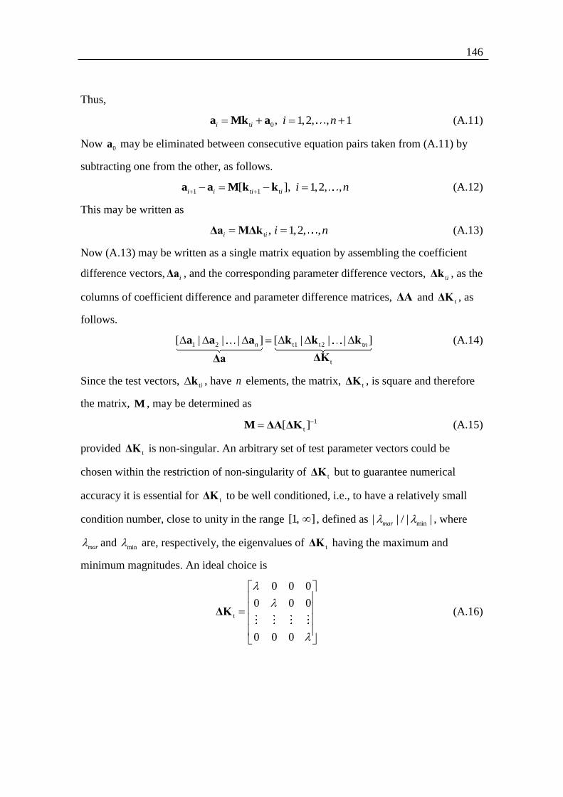
146
Thus,
t 0, 1,2, , 1i i i n a Mk a (A.11)
Now 0a may be eliminated between consecutive equation pairs taken from (A.11) by
subtracting one from the other, as follows.
1 t 1 t[ ], 1,2, ,i i i i i n a a M k k (A.12)
This may be written as
t , 1,2, ,i i i n Δa MΔk (A.13)
Now (A.13) may be written as a single matrix equation by assembling the coefficient
difference vectors, iΔa , and the corresponding parameter difference vectors, tiΔk , as the
columns of coefficient difference and parameter difference matrices, ΔA and tΔK , as
follows.
1 2 t1 t2 t
t
[ | | | ] [ | | | ]n n a a a k k k
ΔKΔa
(A.14)
Since the test vectors, tik , have n elements, the matrix, tΔK , is square and therefore
the matrix, M , may be determined as
1
t[ ]M ΔA ΔK (A.15)
provided tΔK is non-singular. An arbitrary set of test parameter vectors could be
chosen within the restriction of non-singularity of tΔK but to guarantee numerical
accuracy it is essential for tΔK to be well conditioned, i.e., to have a relatively small
condition number, close to unity in the range [1, ] , defined as min| | / | |mar , where
mar and min are, respectively, the eigenvalues of tΔK having the maximum and
minimum magnitudes. An ideal choice is
t
0 0 0
0 0 0
0 0 0
ΔK (A.16)

147
where is a real, non-zero constant. This gives the smallest possible condition number
(i.e., unity) as all the n eigenvalues are equal to and also avoids the matrix inverse in
(A.15) by replacing it with a scalar division by . Thus
1
M ΔA (A.17)
Let the columns of (A.16) be written
1 2
00
0, , ,
0 0
n
λ λ λ (A.18)
Then in view of (A.12), (A.13), (A.14) and (A.16)
t t 1 t , 1,2, ,i i i i i n k k k λ (A.19)
At the beginning, only one test parameter vector has to be chosen. Let this be t1k . Then
the remaining n test parameter vectors can be found from (A.19). Thus
1 , 1,2, ,ti ti i i n k k λ (A.20)
It remains to consider the choice of . It is not actually critical and the calculations are
even simpler by letting 1 since (A.17) becomes just
M ΔA (A.21)

148
A.2.4 Summary of the steps of the numerical pole placement
procedure
Step 1:- Create a SIMULINK block diagram of any system having the desired
closed loop characteristic equation such as in Fig. 10.4
Step 2:- Initialised the coefficient 0nK
Step 3:- and then run the following command in Matlab to get the characteristics
equation of the system by using ‘linmod’, which will give you the state space
equation [A B C D]=linmode(<model name>)
Step 4:- Use the ‘poly’ to get characteristic polynomial coefficients
( )ia poly A
Step 5:- Form the columns, and form the next set of coefficient values for
1n n nK K go to step 3
Step 6:- Calculate the coefficient difference between vectors,
1, 1,2, ,tia a i n from the polynomial
Step 7:- Calculate the vector of desired gains using 1
0[ [ ]]d dK A a a
Step 8:- Now run the Step 3 by using dK and the transfer function should match
the desired closed loop system transfer function
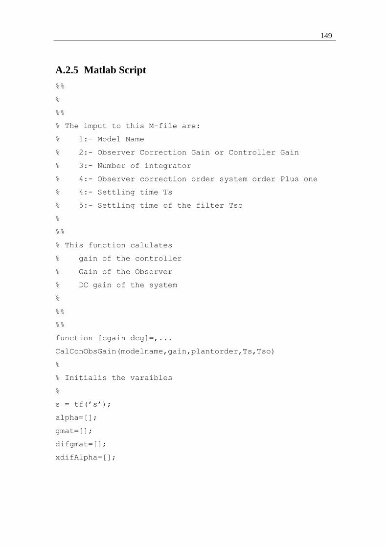
149
A.2.5 Matlab Script
%%
%
%%
% The imput to this M-file are:
% 1:- Model Name
% 2:- Observer Correction Gain or Controller Gain
% 3:- Number of integrator
% 4:- Observer correction order system order Plus one
% 4:- Settling time Ts
% 5:- Settling time of the filter Tso
%
%%
% This function calulates
% gain of the controller
% Gain of the Observer
% DC gain of the system
%
%%
%%
function [cgain dcg]=,...
CalConObsGain(modelname,gain,plantorder,Ts,Tso)
%
% Initialis the varaibles
%
s = tf(’s’);
alpha=[];
gmat=[];
difgmat=[];
xdifAlpha=[];

150
% the overall system shall be observer order which is Plant
or +1;
% the over all system shall be observer order + Plant order
% the obevser
Obserorder=plantorder+1;
Sysorder=Obserorder+plantorder;
% inpk=zeros(norder,1);
inpk=zeros(Sys_order,1);
% create gain difference Matrix
mzero=zeros(Sys_order,Sys_order);
% determine the reference input polynomial coefficients
% since this is associated witht he observer
% the coefficent are calulate
% dusing the observer settling time.
Gob=(s+1.5*(Obser_order+1)/Tso)^Obser_order;
in_coeff= tfdata(Gob,’v’);
%reverse the order of the cofficient fro S^0 to S^n-1.
Input_coeff=in_coeff(length(in_coeff):-1:2);
%%
for i=1:Sys_order;
mzero(i,i)=1;
end
%gmat=rand(norder+1,norder)’;
% replace the above with the difference matrix
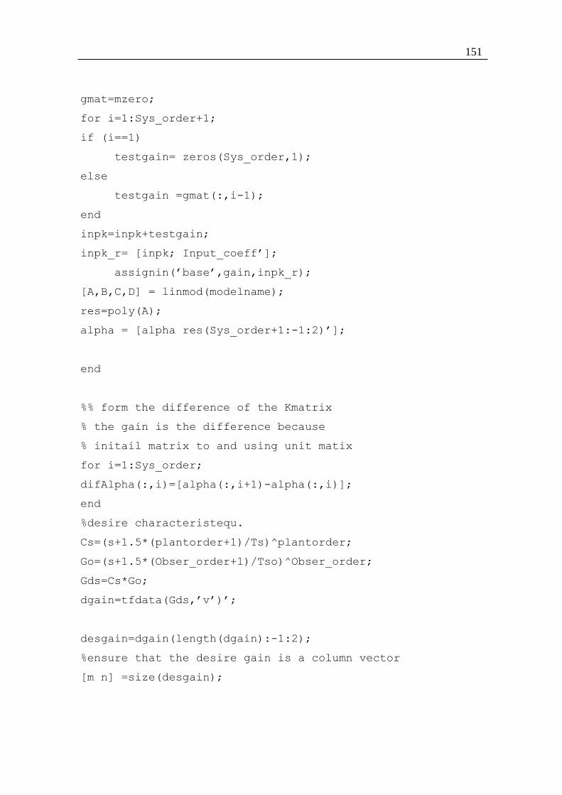
151
gmat=mzero;
for i=1:Sys_order+1;
if (i==1)
testgain= zeros(Sys_order,1);
else
testgain =gmat(:,i-1);
end
inpk=inpk+testgain;
inpk_r= [inpk; Input_coeff’];
assignin(’base’,gain,inpk_r);
[A,B,C,D] = linmod(modelname);
res=poly(A);
alpha = [alpha res(Sys_order+1:-1:2)’];
end
%% form the difference of the Kmatrix
% the gain is the difference because
% initail matrix to and using unit matix
for i=1:Sys_order;
difAlpha(:,i)=[alpha(:,i+1)-alpha(:,i)];
end
%desire characteristequ.
Cs=(s+1.5*(plantorder+1)/Ts)^plantorder;
Go=(s+1.5*(Obser_order+1)/Tso)^Obser_order;
Gds=Cs*Go;
dgain=tfdata(Gds,’v’)’;
desgain=dgain(length(dgain):-1:2);
%ensure that the desire gain is a column vector
[m n] =size(desgain);
152
if (m<n)
desgain=desgain’;
end
% determin the Q matrix
cgain= difAlpha^-1 *(desgain(:,1)-alpha(:,1));
cgain=[cgain;Input_coeff’];
assignin(’base’,gain,cgain);
[A,B,C,D] = linmod(modelname);
sys=tf(ss(A,B,C,D));
dcg=dcgain(sys);
end

153
A.2.6 Polynomial Coefficients
%%
function [Gob fs hs Is dcg]=,...
DeterminLCPIGainVar(TranferFunction,Ts,Tso,IntgTerm,varargi
n)
%
% Dtermine the closed loop gains for the Observer and the
cntroller
% Input to this module is
% Transfer function
% Settling time for the observer and the controller
%%
% Output of this M-file will be
% Controller gain#
% Observer Gains
% correction for the miss match
% make the S as variable
global MinOrder;
s = tf(’s’);
% determine the order of the system
%%
% This routine provides three options.
%%
% Option 1:
%%
% The default setting is to the split the poles
% between the Ts and Tso.
%%
% Option 2:
%%

154
% The User can choose the number of poles
% to be placed at Ts and the
% remianing poles will be placed at Tso.
%%
% Option 3:
%%
% The user will provide a polynominal and
% the remain poles will be palced
% at the TS
%
%% Option 4:
%
% This is the combination of the three
%
%%
% Initialised user define parameter
%%
% Check the additional agreement.
%[Ts : Characteristic equation]
NumberParameterAllow = 6;
NumberOfParameters=nargin;
UseDefaultsetting = 1;
if (NumberOfParameters > NumberParameterAllow)
disp(’Too Many paramter’);
return
end
%
Tfplant=TranferFunction;%*(s^(IntgTerm));
[gnum1 gdnum1]=tfdata(Tfplant,’v’);

155
% Need to ensure the transfer function in standard
% form eg the highest
% power of denomintor is unit.
gnum=gnum1/gdnum1(1);
gdnum=gdnum1/gdnum1(1);
plant_tf=tf(gnum,gdnum);
%Get the Plant order
%%
Porder=length(gdnum)-1;
% assuming the order of the numerator is the same or less
%for the martrix for the d term multiplier
%%
% The overall system will be the plant
% order + observer order (Porder+1);
%
Oborder=Porder;
ClsySOrder=Oborder+Porder;
ClsysCoeff=ClsySOrder+1;
%
% Created the plant order * observer order matrix.
%%
PMat= zeros(ClsySOrder,ClsySOrder);
STermsNumMat= zeros(ClsySOrder,1);
STermsDenMat= zeros(ClsySOrder,1);
GainCoeff =zeros(ClsySOrder,1);
% form the cofficient of the S term which
% of numerator and denomator
%%
156
DenIndexOffset=1;
for i=1:length(gnum)-1;
STermsNumMat(i,1)=gnum(i+DenIndexOffset);
end
for i=1:length(gdnum)-1;
STermsDenMat(i,1)=gdnum(i+DenIndexOffset);
end
% Fill in the matrix with the coefficient of
% the denuminator and numerator.
%%
% in the n
%if (IntgTerm)
for i=1:Oborder;
ShiftRowIndex=i-1;
for j=1:Oborder+1;
PMat(j+ShiftRowIndex,i)=gdnum(j);
end
end
ColIndexOffset=Oborder;
for i=1:Porder+1;
ShiftColIndex=i-1;
for j=1:Porder+1;
PMat(j+ShiftColIndex,i+ColIndexOffset)=gnum(j);
end
end
% determine the reference input polynomial coefficients
% since this is associated witht he observer

157
% the coefficent are calulate
% using the observer settling time withdesire equation.
%%
Gob=(s+1.5*(Oborder+1)/Tso)^Oborder;
%in here we are reversing the data. in_coeff(1)=r0 and so
forth
in_coeff= tfdata(Gob,’v’);
%reverse the order of the cofficient fro S^0 to S^n-1.
RCoeff=in_coeff(length(in_coeff):-1:2);
%
RCoeff=1;
%%;
%desire characteristequ.
%%
DesirDnum =,...
DisredCharacteristicEquat(Ts,Tso,Porder,Oborder,varargin);
% Lets form the the C=Pg
%%
desireCoeff=DesirDnum(2:length(DesirDnum))’;
if (MinOrder)
desireCoeff=DesirDnum’;
CTerm=desireCoeff;
else
desireCoeff=DesirDnum(2:length(DesirDnum))’;
CTerm=desireCoeff-(STermsDenMat+STermsNumMat);

158
end
% Calculate the feed back gains. of the controller
GainCoeff=PMat\CTerm
% To form the closed loop modelis
%%
if (MinOrder)
hden=[GainCoeff(Oborder+1:length(GainCoeff)-
IntgTerm)’];
fden=[GainCoeff(1:Oborder)’];
if(IntgTerm == 0)
Intg=ones(1,IntgTerm+1);
Icoeff=ones(1,IntgTerm+1);
else
Icoeff=[GainCoeff(Oborder+Porder+1:length(GainCoe
ff))’];
Intg=zeros(1,IntgTerm+1);
for i=1:IntgTerm
Intg(i)=1;
end
end
else
hden=[1 GainCoeff(Oborder+1:length(GainCoeff))’];
fden=[1 GainCoeff(1:Oborder)’];
159
Intg=1;
Icoeff=[GainCoeff(Oborder+Porder+1:length(GainCoeff))’
];
end
fs= tf([1],fden);
hs=tf(hden,1);
Is=tf(Icoeff ,Intg);
Gcl= (plant_tf*fs*Is)/(1+fs*hs*plant_tf+ fs*
plant_tf*Is);
% assignin(’base’,GainVectorStrName,cgain);
% [A,B,C,D] = linmodv5(modelname);
% sys=tf(ss(A,B,C,D));
dcg=1/dcgain(Gcl);
end
%%
% return the desired Transfer function
%%
function DessiredChEqu=,...
DisredCharacteristicEquat(ts,tso,porder,oborder,varargin)
global MinOrder;
s=tf(’s’);
if (MinOrder)
porder=porder-1;
oborder=oborder-1;
end

160
NumberOfParameters=length(varargin{:});
switch (length(varargin{:}))
case 0
Gu=1;
case 1
UserParOne=Get_input_Field(NumberOfParameters,1,vararg
in);
[n m]=size(UserParOne);
if (n>1 || m > 1)
NumberOfPole= length(UserParOne)-1;
if (NumberOfPole < oborder)
oborder= oborder-NumberOfPole;
Gu=tf(UserParOne,[1]);
elseif (NumberOfPole < (oborder+podered))
oborder=0
porder= (porder+oborder)-NumberOfPole;
Gu=tf(UserParOne,[1]);
else
oborder=0;
porder=0;
Gu=1;
end
elseif(UserParOne <= porder)
porder=porder-UserParOne;
oborder=oborder+UserParOne;
Gu=1;
else
Gu=1;
oborder=0
porder=0;
161
end
case 2
UserParOne=Get_input_Field(NumberOfParameters,1,v
arargin);
UserParTwo=Get_input_Field(NumberOfParameters,2,v
arargin);
oborder=UserParTwo;
porder=UserParOne;
Gu=1;
% NumberOfPole= length(UserParTwo)-1;
% TotalUserDefinePOles=
NumberOfPole+UserParOne;
% if (TotalUserDefinePOles > oborder)
% oborder=0.
% porder=0;
% Gu=1;
% if((TotalUserDefinePOles-
oborder)<porder)
% porder=porder-
(TotalUserDefinePOles-oborder);
% end
% else
% oborder=oborder-(TotalUserDefinePOles);
% porder=porder+UserParOne;
% Gu=tf(UserParTwo,[1]);
% end
case default
oborder=0.
porder=0;
Gu=1;
end
162
Go=(s+1.5*(oborder+1)/tso)^(oborder);
Cs=(s+1.5*(porder+1)/ts)^porder;
Gds=1/(Go*Cs*Gu);
[DesireNum DessiredChEqu]=tfdata(Gds,’v’);
end
%%
% Gets the parameters from the input arguments vector.
%
function
input_para=Get_input_Field(nb_parameter,index,varargin)
if(index<=nb_parameter)
cell_array=varargin{:};
inpara=cell_array{1};
input_para=inpara{1,index};
else
input_para = ’’;
end
return;
end

163
REFERENCES
[1] A. H. C. D. A. H. E. J. BARNETT, CControl Systems and Control Engineering
Estimators and Observers, Wiki Web, sep 2007.
[2] P. G. BEALE, Lecture notes, http://teal.gmu.edu/ gbeale/examples.html, 2000.
[3] A. K. D.C.MCFARLANE, Robust Controller Design Using Normalised Coprime
Factor Plant Description., Springer-Verlag Lecture Notes in Contytrol and
Information Sciences, jun 1990.
[4] S. J. DODDS, System with different observer design methods, The International
Control Conference..
[5] S. J. DODDS, A novel approach to robust motion control, 5th International
Conference, 2004.
[6] J. D. B. A. T. A. FRANCIS, Feedback ControlTheory, Macmillan Pubishing Co,
1990.
[7] M. A. M. B. P. B. HAJER GHARSALLAOUI, Flatnessbased Control and
Conventional RST Polynomial Control of a Thermal Process, Int.J. of Computers,
Communications & Control, ISSN 1841-9836, E-ISSN 1841-9844, Sept. 2009.
[8] M. HELLSTR´LOM, Engine speed based estimation of the. Master’s thesis, Dept.
of Electrical Engineering, Link´lopings universitet, Feb 2005.
[9] IEEE., State-space solution to standard and control problemvol. Vol.34, IEEE, Aug
1989.
[10] P. G. Z. P. IOAN D. LANDAU, Digital Control System Desing, Identification.
chapter3, 2006..
[11] A. G. K. J.A.SEFTON, Poles-zero cancellation in general problem with refenceto
164
two block design, System and control letters.
[12] H. E. A. K. T. R. JENKINS, Adaptive pole-zero cancellation in grinding, force
control. http://www.deltatau.com/common/support/appex/AllAppex/pmrc5.pdf,
Sept 2005..
[13] C. B. B. JOSEPH, Techniques of Model-Based Control Chapter 2, Prentice Hall,
2002.
[14] S. A. P. M. KAITWANIDVILAI, A genetic-algorithm-based fixedstructure robust
H−∞, SAE Technique paper series, 2002.
[15] A. G. A. C. M.-S. KALMUKALE, Data-based internal model controller design for
a class, European Symposium on Computer Arded Process Engineering (2005).,
2005.
[16] A. KARIMI, Robust control, ECOLE POLYTECHNIQUE FEDERALE DE
LAUSANNE, 2005.
[17] A. LAGERBERG, Control of backlash in automotive powertrains, PhD thesis,
hamers university Sweden, 2004.
[18] A. A. S. B. LAGERBERG, Control of backlash in automotive powertrains, IEEE
Conference , 2009.
[19] I. LANDAU, The R-S-T digital controller design and applications, Control
Engineering Practice 6 1998 155, Dec 1998.
[20] F. S. LEWIS, observer and regulator design, Paper, 2001.
[21] A. F. A. S. S. E. LYNCH, Internal model-based controller design using, paper.
[22] I. THE MATHWORKS, Control Design Course, Sminar version 1.1, Dec 2000.
165
[23] I. THE MATHWORKS, Embedded Torque Estimator for (2004), SAE., SAE.,
2004.
[24] J. J. A. H. P. C. MOSKWA, Engine load torque estimation using vol. 0-7803-2685-
719, IEEE, Proceedings of the 34th.
[25] Q. C. Y. L. H. E. J. NIU, H-infinity control theory in vehicle diesel fuel injection
pump control system design fuel injection systrem, Paper on the Web, Dec 2010.
[26] U. O. E. LONDON, Observer Based Robust Control, Proceedings of Advances in
Computing and Technology, 2007.
[27] J. Kobe, LINEAR DRIVES FOR INDUSTRY APPLICATIONS. Mode of a
Vacuum Air Bearing Linear Drive, 2005.
[28] E. A. G. E. OSTERTAG, RST-Controller Design for Sinewave References
byMeans of an Auxiliary Diophantine Equation, 44th IEEE Conference, Dec 2005.
[29] E. A. G. E. OSTERTAG, Rst-conttroller design a ratinal teaching mehtod based on
two diophantine equation, Control Engineering Practice , Dec 2006.
[30] G. F. A. G. L. PAOLO FALCONE, Non-linear net engine torque estimator,
http://web.ing.unisannio.it/fiengo/Download/Pers/Torque, 2005.
[31] D. SIMON, Analyzing control system robustness, sept 2008.
[32] A. R. S.J.WILLIAMS, A comparison of different h-infinity design methods for
vstol flight control system design, San Diego: In American Control Conference pp.
2508–2513, May 1990.
[33] S. A. P. I. SKOGESTAD, Multivariable feedback Control Analysis and design,
Jonn Wiley and Sons, 1993.
[34] N. S.NISE, Control Systems Engineerin, 2nd edition Chapter7.7, Road,Menlo
166
Park,CA: Addison-Welsely, 2725 Sand Hill, 1995.
[35] S.Dodds, Settling time formulae for the design of control systems with linear
closed loop dynamics, UNIVERSITY OF EAST LONDON., 2008.
[36] G. VAN DER ZALM, DEVELOPMENT OF A TUNING METHOD FOR SPEED
CONTROLLERSIN DAF TRUCKS, DAF-report nr. 51051/04-049 , June 2004.
[37] J. A. D. S. J. VITTEK, Forced Dynamic Control of Electric Drives, University of
Zilina Press,book ISBN 80-8070-087-7, 2003.
[38] G. A. B. G. WELCH, An Introduction to the Kalman Filter’. University of, Chapel
Hil : University of North Carolina , 2005.
[39] P. J. Maloney, Embedded Torque Estimator for Diesel Engine Control Application,
SAE International, 2004 .
[40] M. A. F. K. G. Javier Francoa, Real-time brake torque estimation for internal
combustion engines, Mechanical Systems and Signal Processing 22 338–361,
2008.
[41] J. e. a. Doyle, State-Space Solutions to Standard HS and H-infinity Control
Problems, IEEE Transactions on Automatic Control 34.8 , 1990.
[42] J. K. G. P. K. a. B. F. Doyle, State-Space Solutions to Standard HS and H-infinity
Control Problems, IEEE Transactions on Automatic Control 34, no. 8, 1989.
[43] B. F. A. T. John Doyle, Feedback Control Theory, Macmillan Publishing co, 1990.
[44] D. E. Rivera, Internal Model Control, College of Engineering and Applied
Sciences Arizona State University Tempe, Arizona 85287-6006.
[45] D. M. M. a. S. S. Rivera, Internal Model Control 4. PID Controller, Ind. Eng.
Chem. Process Des. Dev. 25, 252, , 1986.

167
[46] M. S. a. M. Lee, IMC Filter Design for PID Controller Tuning of Time Delayed
Processes, 2012.
[47] M. a. E. Z. Morari, Robust Process Control, NY: Prentice-Hall, Englewood Cliffs,
1989.
[48] M. T. Tham, “Internal model control,” Chemical and Process Eng, University of
Newcaslte upon Tyne, 2002.
[49] Y. H. D. ZWEIRI, “engine indicated torque estimation based,” vol. VOLUME 1,
June 2006.
[50] R.F.HARRISON, “Robust and Mutivariable Control,” Msc Lecuture notes of
University Of Sheffield , Sept 2000.
[51] D. SIMON, “H-infinity filtering with inequality constraints for aircraft turbofan
engine health estimation,” ECOLE POLYTECHNIQUE FEDERALE DE
LAUSANNE, Sept 2005.
[52] J. D. C. J. S. M. V. P. SAS, “H-infinity feedback control for signal tracking on a 4
poster testrig in the automotive industry,” 2002.
[53] G. Rizzoni, “Estimate of IC Engine Torque from Measurement of Crankshaft
Angular Position,” Sept 1993.
[54] B. Lee, G. Rizzoni, Y. Guezennec and A. Soliman, Engine Control Using Torque
Estimation, SAE TECHNICAL, 2001.
[55] B. LEE, G. Y. G. RIZZONI and A. S. A. , “Engine control using torque
estimation.,” 2001.
[56] R. N. CLARK, “Another reason to eschew pole-zero,” April 988.
[57] K. ASTROM and B. WITTENMARK, Control system Theory and design chapter
168
10, NY: Parentice-Hall.
[58] A. K and B. WITTENMARK, Control system Theory and design, Computers
Communications & Control, 2009.
[59] B. S.W.S.J and P. L. LEE, “Passivity based imc control for multivariable
nonlinear,” 2005.
[60] A. H. BARNETT, M. BLAAUBOER, A. MODY and E. J. AND HELLER,
“dynamics of air-breathing hypersonic. Flight path angle,” paper, 2004.
[61] Y. H. Zweiri, “Diesel Engine Indicated Torque Estimation Based on Artificial
Neural Networks,” no. 1.
[62] K.J.HUNT, R.P.JAIME and H.GOLLEE., “Robust control of electrically-
Stimulated Muscle using Polnomial H_infinity design,” University of Glasgow,
2004.
[63] X.-D. SUN, P. G. Scots. and G. BALFOUR, “Application of loop shaping H-
infinity control to diesel engine control,” Mar 2002.