1

Robust Attitude Tracking for Aerobatic Helicopters:A Geometric Approach

Nidhish Raj, Ravi N Banavar, Abhishek, and Mangal Kothari

Abstract—This paper highlights the significance of the rotordynamics in control design for small-scale aerobatic helicopters,and proposes two singularity free robust attitude tracking con-trollers based on the available states for feedback. 1. The first,employs the angular velocity and the flap angle states (a variablethat is not easy to measure) and uses a backstepping techniqueto design a robust compensator (BRC) to actively suppress thedisturbance induced tracking error. 2. The second exploits theinherent damping present in the helicopter dynamics leading toa structure preserving, passively robust controller (SPR), whichis free of angular velocity and flap angle feedback. The BRCcontroller is designed to be robust in the presence of two typesof uncertainties: structured and unstructured. The structureddisturbance is due to uncertainty in the rotor parameters, andthe unstructured perturbation is modeled as an exogenous torqueacting on the fuselage. The performance of the controller isdemonstrated in the presence of both types of disturbancesthrough numerical simulations. In contrast, the SPR trackingcontroller is derived such that the tracking error dynamics inher-its the natural damping characteristic of the helicopter. The SPRcontroller is shown to be almost globally asymptotically stableand its performance is evaluated experimentally by performingaggressive flip maneuvers. Throughout the study, a nonlinearcoupled rotor-fuselage helicopter model with first order flapdynamics is used.

Index Terms—Geometric Control, Attitude Tracking, Heli-copter, Robust Control.

I. INTRODUCTION

SMALL-SCALE helicopters with a single main rotor and atail rotor are capable of performing extreme 3D aerobatic

maneuvers [1]–[3]. These aggressive maneuvers involve largeangle rotations with high angular velocity, inverted flight, split-S, pirouette etc. This necessitates a robust attitude trackingcontroller which is globally defined and is capable of achievingsuch aggressive rotational maneuvers.

The attitude tracking problem of a helicopter is significantlydifferent from that of a rigid body. A small-scale helicopteris modeled as a coupled interconnected system consisting ofa fuselage and a rotor. The control moments generated by therotor excite the rigid body dynamics of the fuselage which in-turn affects the rotor loads and its dynamics causing nonlinearcoupling. The key differences between the rigid body trackingproblem and the attitude tracking of a helicopter are thefollowing: 1) the presence of large aerodynamic damping inthe rotational dynamics and 2) the required control moment

This work was funded by the Department of Science and Technology, India.Nidhish Raj, Abhishek, and Mangal Kothari are with the Department of

Aerospace Engineering, Indian Institute of Technology Kanpur, UP, 208016India e-mail: (nraj,abhish,mangal)@iitk.ac.in.

Ravi N Banavar is with the Systems and Control Engineering, IndianInstitute of Technology Bombay, Mumbai, India e-mail: banavar@iitb.ac.in.

for tracking cannot be applied instantaneously due to the rotorblade dynamics. The control moments are produced by therotor subsystem which, for the purpose of attitude tracking,can be approximated as a first order system [4]. The dampingintroduced by the rotor subsystem does not hamper attitudestabilization or slow trajectory tracking. But it becomes aserious impediment for fast aerobatic maneuvers, which iswhat has been addressed in this article. This is in contrastto a quadrotor, where the rigid body approximation is close tothe actual dynamics due to relatively small rotors.

A. Related Work

The significance of including the rotor dynamics in con-troller design for helicopters has been extensively studiedin the literature [5]–[8]. Hall Jr and Bryson Jr [5] haveshown the importance of rotor state feedback in achievingtight attitude control for large scale helicopters, Takahashi [6]compares H∞ attitude controller design for the cases withand without rotor state feedback. In a similar work, Ingleand Celi [7] have investigated the effect of including rotordynamics on various controllers, namely LQG, EigenstructureAssignment and H∞, for meeting stringent handling qualityrequirements. They conclude that the controllers designed tomeet the high bandwidth requirements with the rotor dynamicswere more robust and required lower control activity than theones designed without including the rotor dynamics. Panzaand Lovera [8] used rotor state feedback and designed an H∞controller which is robust and also fault tolerant with respectto failure of the rotor state sensor. Previous attempts to small-scale helicopter attitude control are mostly based on attitudeparametrization such as Euler angles, which suffer from sin-gularity issues, or quaternions which have ambiguity in repre-sentation. Tang, Yang, Qian, and Zheng [9] explicitly considerthe rotor dynamics and design stabilizing controller based onsliding mode technique using Euler angles and hence confinedto small angle maneuvers. Raptis, Valavanis, and Moreno[10] have designed position tracking controller for small-scalehelicopter wherein the inner loop attitude controller was basedon rotation matrix, but does not consider the rotor dynamics.Marconi and Naldi [11], [12] designed a position trackingcontroller for flybared (with stabilizer bar) miniature helicopterwhich is robust with respect to large variations in parameters,but have made the simplifying assumption of disregardingthe rotor dynamics by taking a static relation between theflap angles and the cyclic input. Stressing the significanceof rotor dynamics, Ahmed and Pota [13], [14] developed abackstepping based stabilizing controller using Euler angles

arX

iv:1

709.

0565

2v2

[cs

.SY

] 9

Jan

201

9

2

for a small-scale flybared helicopter with the inclusion ofservo and rotor dynamics. They have provided correctionterms in the controller to incorporate the effect of servo androtor dynamics. For near hover conditions, Zhu and Huo [15]have developed a robust nonlinear controller disregarding theflap dynamics. Frazzoli, Dahleh, and Feron [16] developed acoordinate chart independent trajectory tracking controller onthe configuration manifold SE(3) for a small-scale helicopter,but the flap dynamics, critical for accurate representation ofthe system, was not taken into account.

B. Contribution

The present work emphasizes on the inclusion of therotor dynamics in the design of attitude tracking controllerfor small scale aerobatic helicopters. It is an improvementover the simple attitude tracking controller proposed by theauthors in [17]. The backstepping technique employed in theprevious work warranted the removal of damping term fromthe dynamics for performing aggressive maneuvers. As shownin Sec V, uncertainties in the rotor time constant estimate, τm,or its variation with vehicle operating condition could result inexcess removal of damping, thereby injecting energy into thesystem and making the closed loop unstable. The novelty ofthe present work is in the design of two singularity free attitudetracking controllers which are robust to the aforementionedparametric variation. The first controller uses backsteppingtechnique to design a robust compensator to actively suppressthe disturbance induced tracking error. Disturbance enteringinto the system due to uncertainty in parameters is termedstructured uncertainty. In addition, the effect of a time varyingexogenous torque acting on the fuselage is also considered andis lumped together as ∆f (t) in (1), hence termed unstruc-tured. The proposed BRC controller ensures robustness to bothuncertainties and renders the solutions of the associated errordynamics to be uniformly ultimately bounded. It is observedthrough numerical simulations that the proposed controller iscapable of performing aggressive rotational maneuvers in thepresence of the aforementioned structured and unstructureddisturbances. The disadvantage of this controller is the needfor, difficult to measure, flap angle state for feedback. Onthe other hand, the second controller is derived such thatthe tracking error dynamics inherits the natural dampingcharacteristic of the helicopter. This avoids the unnecessarycancellation of inherent damping, thereby making it robust.This controller has the added advantage of being free of flapand angular velocity feedback and hence easily implementable.On the downside, due to the passive nature of its robustness,the controller cannot confine the tracking error to prescribedlimits. The performance of the controller is proven throughexperiments by performing aggressive flip maneuvers on asmall scale helicopter.

The paper is organized as follows: Section II describes therotor-fuselage dynamics of a small-scale helicopter, explainsthe effect of aerodynamic damping, and motivates the needfor a robust attitude tracking controller. Section III presentsthe backstepping based robust attitude tracking controller.The efficacy of the BRC controller is demonstrated through

a

b

Xb

Yb

Zb

Xe

Ye

Ze

Hub plane

Rotor disc

Fuselage

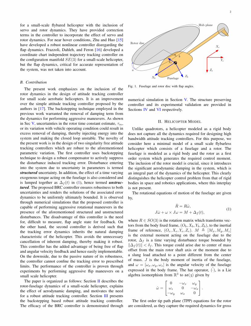
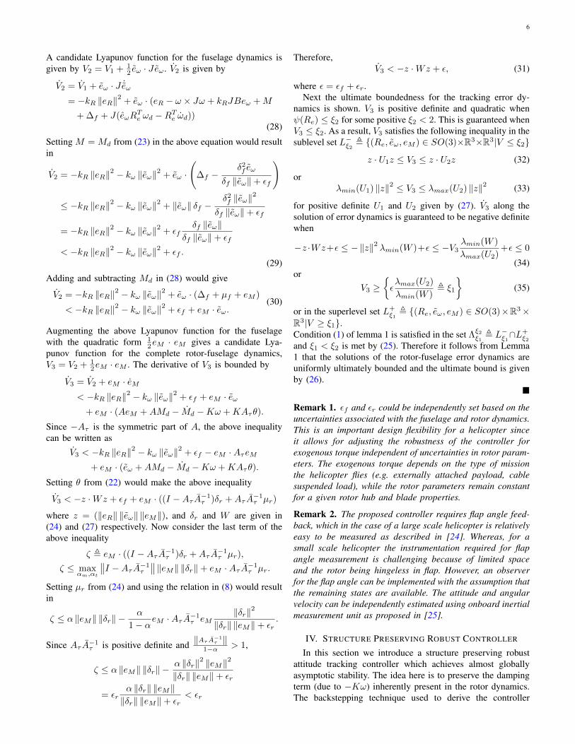
Fig. 1. Fuselage and rotor disc with flap angles.

numerical simulation in Section V. The structure preservingcontroller and its experimental validation are provided inSections IV and VI respectively.

II. HELICOPTER MODEL

Unlike quadrotors, a helicopter modeled as a rigid bodydoes not capture all the dynamics required for designing highbandwidth attitude tracking controllers. For this purpose, weconsider here a minimal model of a small scale flybarlesshelicopter which consists of a fuselage and a rotor. Thefuselage is modeled as a rigid body and the rotor as a firstorder system which generates the required control moment.The inclusion of the rotor model is crucial, since it introducesthe significant aerodynamic damping in the system, which isan integral part of the dynamics of the helicopter. This clearlydistinguishes the helicopter control problem from that of rigidbodies in space and robotics applications, where this interplayis not present.

The rotational equations of motion of the fuselage are givenby,

R = Rω,

Jω + ω × Jω = M + ∆f (t),(1)

where R ∈ SO(3) is the rotation matrix which transforms vec-tors from the body fixed frame, (Ob, Xb, Yb, Zb), to the inertialframe of reference, (Oe, Xe, Ye, Ze). M , [Mx,My,Mz]is the external moment acting on the fuselage due to therotor, ∆f is a time varying disturbance torque bounded by‖∆f (t)‖ < δf . This torque could arise due to center of massoffset from the main rotor shaft axis or the moment due toa slung load attached to a point different from the centerof mass. J is the body moment of inertia of the fuselage,and ω = [ωx, ωy, ωz] is the angular velocity of the fuselageexpressed in the body frame. The hat operator, (·), is a Liealgebra isomorphism from R3 to so(3) given by

ω =

0 −ωz ωyωz 0 −ωx−ωy ωx 0

.The first order tip path plane (TPP) equations for the rotor

are considered, as they capture the required dynamics for gross

3

movement of the fuselage [4]. The coupled flap equation fora counter-clockwise rotor are given by [4], [18]

a = − 1

τma+

kβ2ΩIβ

b− ωy +1

τm

(θa −

ωxΩ

),

b = − 1

τmb− kβ

2ΩIβa− ωx +

1

τm

(θb +

ωyΩ

).

(2)

where a and b are respectively the longitudinal and lateral tiltof the rotor disc with respect to the hub plane as shown in Fig.1. τm is the main rotor time constant and θa and θb are thecontrol inputs to the rotor subsystem. They are respectivelythe lateral and longitudinal cyclic blade pitch angles actuatedby servos through a swash plate mechanism. kβ is the bladeroot stiffness, Ω is the main rotor angular velocity, and Iβ isthe blade moment of inertia about the flap hinge. The aboveequation introduces cross coupling through flap angle andangular velocity. Note that the effect of the angular velocitycross coupling can be effectively canceled using the fuselageangular velocity feedback, since the rotor angular velocity, Ω,can be measured accurately using an on-board autopilot.

The coupling of rotor and fuselage occurs through the rotorhub. The rolling moment, Mx and pitching moment My , actingon the fuselage due to the rotor flapping consists of twocomponents – due to tilting of the thrust vector, T , and dueto the rotor hub stiffness, kβ , and are given by

Mx = (hT + kβ)b,

My = (hT + kβ)a,(3)

where h is the distance of the rotor hub from the center ofmass. For small-scale helicopters, the rotor hub stiffness kβ ismuch larger than the component due to tilting of thrust vector,hT (see Table I). Thus, a nominal variation in thrust wouldresult in only a small variation of the equivalent hub stiffness,Kβ , (hT + kβ). The control moment about yaw axis, Mz ,is applied through tail rotor which, due to it’s higher RPM,has a much faster aerodynamic response than the main rotorflap dynamics. The tail rotor along with the actuating servo ismodeled as a first order system with τt as the tail rotor timeconstant,

Mz = −Mz/τt −Ktωz +KtKt0θt/τt, (4)

where Kt0 relates the steady state yaw rate to control input,θt.

The main rotor dynamics (2) and tail rotor dynamics couldbe written in terms of the control moments and a pseudo-control input θ , [θb + ωy/Ω, θa − ωx/Ω,Kt0θt] as,

M = AM −Kω +KAτθ, (5)

where

A ,

−1/τm −k 0k −1/τm 00 0 −1/τt

, (6)

Aτ , diag(1/τm, 1/τm, 1/τt), K , diag(Kβ ,Kβ ,Kt),k , kβ/(2ΩIβ), and M , [Mx,My,Mz]. The symmetricand skew symmetric parts of A are denoted by −Aτ and Akrespectively. Note that the combined rotor-fuselage dynamicsgiven by (1) and (5) cannot be given the form of a simple

0 1 2 3 4 5

-200

-100

0

100

200Angular Velocity (deg/s)

exp x

sim x

exp y

sim y

0 1 2 3 4 5Time (s)

-10

-5

0

5

10Control Input (deg)

b a

(a)

0 0.5 1 1.5 2

-200

-100

0

100

200Angular Velocity (deg/s)

exp x

sim x

exp y

sim y

0 0.5 1 1.5 2Time (s)

-10

-5

0

5

10Control Input (deg)

b a

(b)

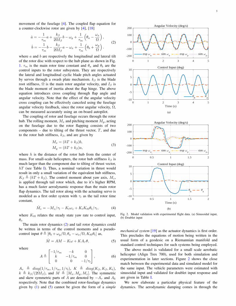
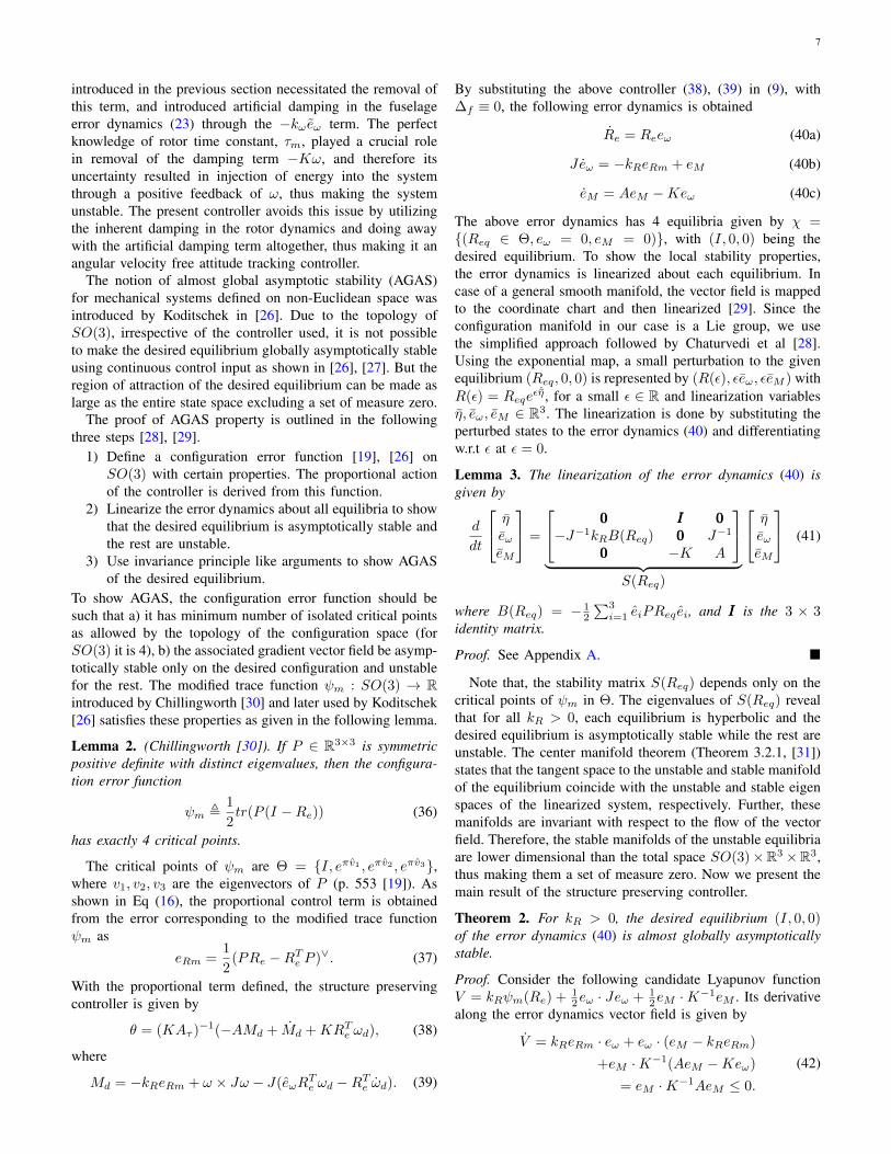
Fig. 2. Model validation with experimental flight data. (a) Sinusoidal input,(b) Doublet input

mechanical system [19] as the actuator dynamics is first order.This precludes the equations of motion being written in theusual form of a geodesic on a Riemannian manifold andstandard control techniques for such systems being employed.

The above model is validated for a small scale aerobatichelicopter (Align Trex 700), used for both simulation andexperimentation in later sections. Figure 2 shows the closematch between the experimental data and simulated model forthe same input. The vehicle parameters were estimated withsinusoidal input and validated for doublet input response andare given in Table I.

We now elaborate a particular physical feature of thedynamics. The aerodynamic damping comes in through the

4

0 0.2 0.4 0.6 0.8 1-180

-90

0

90

180

270

360

Angular Velocity (deg/s)

x y

0 0.2 0.4 0.6 0.8 1

Time (s)

-20

-10

0

10Damping Moment (N-m)

Mx

My

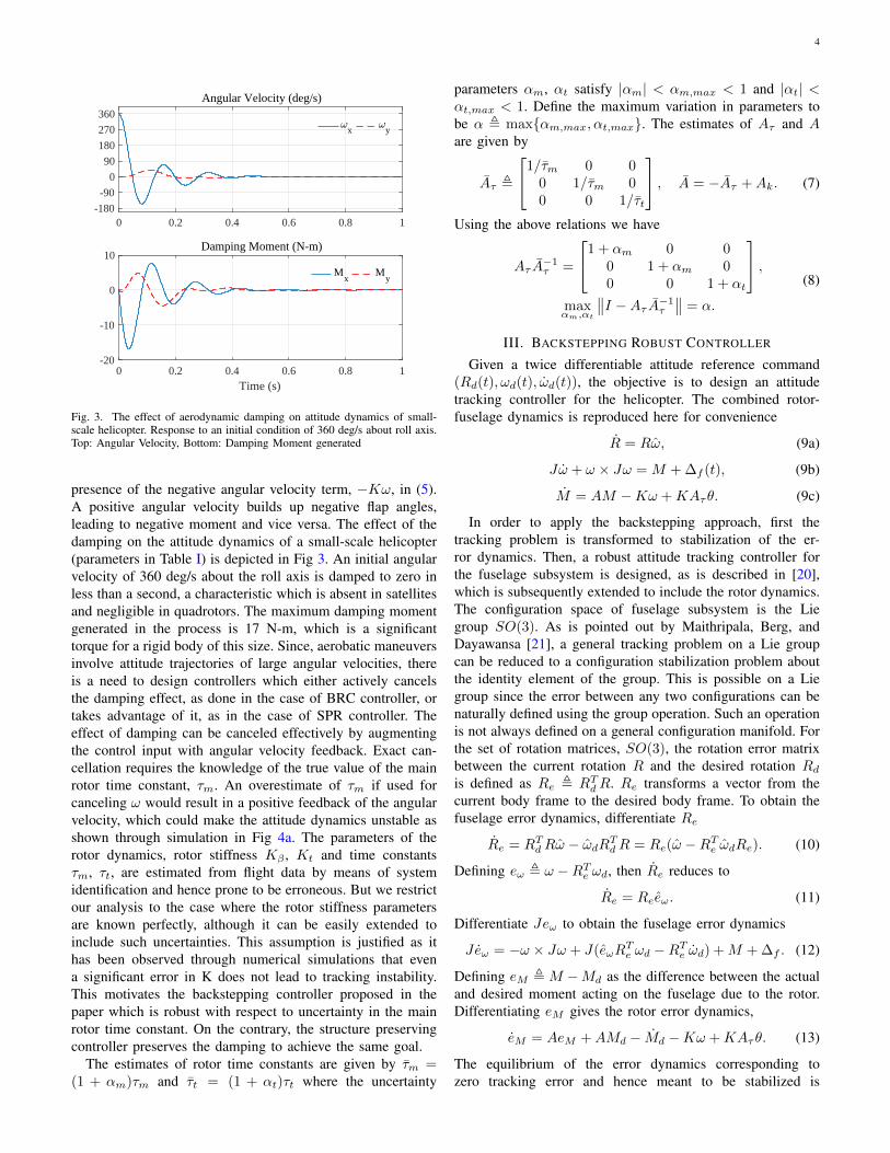
Fig. 3. The effect of aerodynamic damping on attitude dynamics of small-scale helicopter. Response to an initial condition of 360 deg/s about roll axis.Top: Angular Velocity, Bottom: Damping Moment generated

presence of the negative angular velocity term, −Kω, in (5).A positive angular velocity builds up negative flap angles,leading to negative moment and vice versa. The effect of thedamping on the attitude dynamics of a small-scale helicopter(parameters in Table I) is depicted in Fig 3. An initial angularvelocity of 360 deg/s about the roll axis is damped to zero inless than a second, a characteristic which is absent in satellitesand negligible in quadrotors. The maximum damping momentgenerated in the process is 17 N-m, which is a significanttorque for a rigid body of this size. Since, aerobatic maneuversinvolve attitude trajectories of large angular velocities, thereis a need to design controllers which either actively cancelsthe damping effect, as done in the case of BRC controller, ortakes advantage of it, as in the case of SPR controller. Theeffect of damping can be canceled effectively by augmentingthe control input with angular velocity feedback. Exact can-cellation requires the knowledge of the true value of the mainrotor time constant, τm. An overestimate of τm if used forcanceling ω would result in a positive feedback of the angularvelocity, which could make the attitude dynamics unstable asshown through simulation in Fig 4a. The parameters of therotor dynamics, rotor stiffness Kβ , Kt and time constantsτm, τt, are estimated from flight data by means of systemidentification and hence prone to be erroneous. But we restrictour analysis to the case where the rotor stiffness parametersare known perfectly, although it can be easily extended toinclude such uncertainties. This assumption is justified as ithas been observed through numerical simulations that evena significant error in K does not lead to tracking instability.This motivates the backstepping controller proposed in thepaper which is robust with respect to uncertainty in the mainrotor time constant. On the contrary, the structure preservingcontroller preserves the damping to achieve the same goal.

The estimates of rotor time constants are given by τm =(1 + αm)τm and τt = (1 + αt)τt where the uncertainty

parameters αm, αt satisfy |αm| < αm,max < 1 and |αt| <αt,max < 1. Define the maximum variation in parameters tobe α , maxαm,max, αt,max. The estimates of Aτ and Aare given by

Aτ ,

1/τm 0 00 1/τm 00 0 1/τt

, A = −Aτ +Ak. (7)

Using the above relations we have

Aτ A−1τ =

1 + αm 0 00 1 + αm 00 0 1 + αt

,maxαm,αt

∥∥I −Aτ A−1τ

∥∥ = α.

(8)

III. BACKSTEPPING ROBUST CONTROLLER

Given a twice differentiable attitude reference command(Rd(t), ωd(t), ωd(t)), the objective is to design an attitudetracking controller for the helicopter. The combined rotor-fuselage dynamics is reproduced here for convenience

R = Rω, (9a)

Jω + ω × Jω = M + ∆f (t), (9b)

M = AM −Kω +KAτθ. (9c)

In order to apply the backstepping approach, first thetracking problem is transformed to stabilization of the er-ror dynamics. Then, a robust attitude tracking controller forthe fuselage subsystem is designed, as is described in [20],which is subsequently extended to include the rotor dynamics.The configuration space of fuselage subsystem is the Liegroup SO(3). As is pointed out by Maithripala, Berg, andDayawansa [21], a general tracking problem on a Lie groupcan be reduced to a configuration stabilization problem aboutthe identity element of the group. This is possible on a Liegroup since the error between any two configurations can benaturally defined using the group operation. Such an operationis not always defined on a general configuration manifold. Forthe set of rotation matrices, SO(3), the rotation error matrixbetween the current rotation R and the desired rotation Rdis defined as Re , RTdR. Re transforms a vector from thecurrent body frame to the desired body frame. To obtain thefuselage error dynamics, differentiate Re

Re = RTdRω − ωdRTdR = Re(ω −RTe ωdRe). (10)

Defining eω , ω −RTe ωd, then Re reduces to

Re = Reeω. (11)

Differentiate Jeω to obtain the fuselage error dynamics

Jeω = −ω × Jω + J(eωRTe ωd −RTe ωd) +M + ∆f . (12)

Defining eM ,M −Md as the difference between the actualand desired moment acting on the fuselage due to the rotor.Differentiating eM gives the rotor error dynamics,

eM = AeM +AMd − Md −Kω +KAτθ. (13)

The equilibrium of the error dynamics corresponding tozero tracking error and hence meant to be stabilized is

5

(Re, eω, eM ) = (I, 0, 0). The tracking error stabilizing con-troller has proportional derivative plus feed-forward compo-nents. The proportional action is derived from a tracking errorfunction ψ : SO(3)→ R which is defined as

ψ(Re) ,1

2tr[I −Re]. (14)

ψ has a single critical point within the sub level set about theidentity I, Γ2 , R ∈ SO(3)|ψ(R) < 2. This sublevel setrepresents the set of all rotations which are less than π radiansfrom the identity I . The derivative of ψ is given by

d

dtψ(Re(t)) =

1

2tr(−Re(t)) = −1

2tr(Reeω)

= −1

2tr

(1

2(Re −RTe )eω

)= eR · eω,

(15)

where the rotation error vector is

eR ,1

2[Re −RTe ]∨, (16)

where (·)∨ : so(3) → R3 is the inverse of hat map (·). Theabove derivation uses the fact that − 1

2 tr(ab) = a · b andthe trace of the product of symmetric and skew symmetricmatrices is zero. The total derivative of eR is

eR =1

2(Re − RTe )∨ =

1

2(Reeω + eωR

Te )∨

= B(Re)eω,(17)

where B(Re) , 12 [tr(RTe )I − RTe ]. Since ψ is positive

definite and quadratic within the sub level set Γξ2 , R ∈SO(3)|ψ(R) ≤ ξ2 for some positive ξ2 < 2, this makes ψuniformly quadratic about the identity [19]. This implies thereexists positive constants b1 = 1/2 and b2 = 1/(2 − ξ2) [22]such that

b1 ‖eR‖2 ≤ ψ(R) ≤ b2 ‖eR‖2 . (18)

The following definition of ultimate boundedness takenfrom [23] has been given here for the sake of completeness.

Definition 1. Consider the system

x = f(t, x) (19)

where f : [0,∞) × D → Rn is piecewise continuous in tand locally Lipschitz in x on [0,∞) × D, and D ⊂ Rncontains the origin (equilibrium). The solutions of (19) areuniformly ultimately bounded with ultimate bound b if thereexist positive constants b and c, independent of t0, and forevery a ∈ (0, c), there is T = T (a, b) ≥ 0, independent of t0,such that

‖x(t0)‖ ≤ a =⇒ ‖x(t)‖ ≤ b, ∀t ≥ t0 + T. (20)

The following lemma uses Lyapunov analysis to showultimate boundedness for (19) and is a variation of Theorem4.18 in [23].

Lemma 1. ( [23]) Let D ⊂ Rn be a domain that containsthe origin and V : [0,∞) × D → R be a continuouslydifferentiable function such that

k1 ‖x‖2 ≤ V (t, x) ≤ k2 ‖x‖2 , V ≤ −k3 ‖x‖2

∀x ∈ Λc2c1 , x ∈ D|c1 ≤ V ≤ c2, 0 < c1 < c2, ∀t ≥ 0,

for positive k1, k2, k3 and consider the sublevel set L−c2 ,x ∈ Rn|V ≤ c2 ⊂ D. Then, for every initial conditionx(t0) ∈ L−c2 , the solution of (19) is uniformly ultimatelybounded with ultimate bound b, i.e. there exists T ≥ 0 suchthat

‖x(t)‖ ≤(k2

k1

)1/2

‖x(t0)‖ e−γ(t−t0), ∀t0 ≤ t ≤ t0 + T

(21a)‖x(t)‖ ≤ b, ∀t ≥ t0 + T (21b)

where γ = k32k2

, b =(c1k1

)1/2

.

The proof is straightforward. The following theorem presentsthe backstepping robust controller.

Theorem 1. For all initial conditions starting in the set S ,(Re, eω, eM ) ∈ SO(3) × R3 × R3|ψ(Re) + 1

2 eω · Jeω +12eM · eM ≤ ξ2 for a positive ξ2 < 2, the solutions of theerror dynamics (11), (12), and (13) are rendered uniformlyultimately bounded by the following choice of control input

θ = (KAτ )−1(−AMd + Md − eω +Kω + µr), (22)

where eω = eω + kReR,

Md = −kω eω − eR − kRJBeω + ω × Jω−J(eωR

Te ωd −RTe ωd) + µf ,

µf =−δ2

f eω

δf ‖eω‖+ εf,

(23)

µr =−α

1− α‖δr‖2 eM

‖δr‖ ‖eM‖+ εr,

δr = eω +AkMd − Md −Kω,(24)

for some kR > 0, kω > 0 and εf > 0, εr > 0 such that

ε , εf + εr < ξ2λmin(W )

λmax(U2). (25)

The ultimate bound is given by

b =

(λmax(U2)

λmin(U1)λmin(W )ε

)1/2

. (26)

The matrices U1, U2 and W are given by

U1 ,1

2

1 0 00 λmin(J) 00 0 1

, U2 ,1

2

22−ξ2 0 0

0 λmax(J) 00 0 1

,W ,

kR 0 00 kω 00 0 λmin(Aτ )

.(27)

Proof. Consider the following positive definite quadratic func-tion in the sublevel set Γξ2 , V1 , ψ. The time derivative of thisfunction, V1 = eR ·eω , can be made negative definite by settingthe virtual control input eω = −kReR. A change of variableeω = eω + kReR would make V1 = −kR ‖eR‖2 + eR · eω .The error dynamics for eω is given by

˙eω = eω + kReR

= J−1(−ω × Jω + J(eωRTe ωd −RTe ωd)

+M + ∆f ) + kRBeω.

6

A candidate Lyapunov function for the fuselage dynamics isgiven by V2 = V1 + 1

2 eω · Jeω . V2 is given by

V2 = V1 + eω · J ˙eω

= −kR ‖eR‖2 + eω · (eR − ω × Jω + kRJBeω +M

+ ∆f + J(eωRTe ωd −RTe ωd))

(28)

Setting M = Md from (23) in the above equation would resultin

V2 = −kR ‖eR‖2 − kω ‖eω‖2 + eω ·

(∆f −

δ2f eω

δf ‖eω‖+ εf

)

≤ −kR ‖eR‖2 − kω ‖eω‖2 + ‖eω‖ δf −δ2f ‖eω‖

2

δf ‖eω‖+ εf

= −kR ‖eR‖2 − kω ‖eω‖2 + εfδf ‖eω‖

δf ‖eω‖+ εf

< −kR ‖eR‖2 − kω ‖eω‖2 + εf .(29)

Adding and subtracting Md in (28) would give

V2 = −kR ‖eR‖2 − kω ‖eω‖2 + eω · (∆f + µf + eM )

< −kR ‖eR‖2 − kω ‖eω‖2 + εf + eM · eω.(30)

Augmenting the above Lyapunov function for the fuselagewith the quadratic form 1

2eM · eM gives a candidate Lya-punov function for the complete rotor-fuselage dynamics,V3 = V2 + 1

2eM · eM . The derivative of V3 is bounded by

V3 = V2 + eM · eM< −kR ‖eR‖2 − kω ‖eω‖2 + εf + eM · eω

+ eM · (AeM +AMd − Md −Kω +KAτθ).

Since −Aτ is the symmetric part of A, the above inequalitycan be written as

V3 < −kR ‖eR‖2 − kω ‖eω‖2 + εf − eM ·AτeM+ eM · (eω +AMd − Md −Kω +KAτθ).

Setting θ from (22) would make the above inequality

V3 < −z ·Wz + εf + eM · ((I −Aτ A−1τ )δr +Aτ A

−1τ µr)

where z = (‖eR‖ ‖eω‖ ‖eM‖), and δr and W are given in(24) and (27) respectively. Now consider the last term of theabove inequality

ζ , eM · ((I −Aτ A−1τ )δr +Aτ A

−1τ µr),

ζ ≤ maxαm,αt

∥∥I −Aτ A−1τ

∥∥ ‖eM‖ ‖δr‖+ eM ·Aτ A−1τ µr.

Setting µr from (24) and using the relation in (8) would resultin

ζ ≤ α ‖eM‖ ‖δr‖ −α

1− αeM ·Aτ A−1

τ eM‖δr‖2

‖δr‖ ‖eM‖+ εr.

Since Aτ A−1τ is positive definite and ‖Aτ A

−1τ ‖

1−α > 1,

ζ ≤ α ‖eM‖ ‖δr‖ −α ‖δr‖2 ‖eM‖2

‖δr‖ ‖eM‖+ εr

= εrα ‖δr‖ ‖eM‖‖δr‖ ‖eM‖+ εr

< εr

Therefore,V3 < −z ·Wz + ε, (31)

where ε = εf + εr.Next the ultimate boundedness for the tracking error dy-

namics is shown. V3 is positive definite and quadratic whenψ(Re) ≤ ξ2 for some positive ξ2 < 2. This is guaranteed whenV3 ≤ ξ2. As a result, V3 satisfies the following inequality in thesublevel set L−ξ2 , (Re, eω, eM ) ∈ SO(3)×R3×R3|V ≤ ξ2

z · U1z ≤ V3 ≤ z · U2z (32)

orλmin(U1) ‖z‖2 ≤ V3 ≤ λmax(U2) ‖z‖2 (33)

for positive definite U1 and U2 given by (27). V3 along thesolution of error dynamics is guaranteed to be negative definitewhen

−z ·Wz+ε ≤ −‖z‖2 λmin(W )+ε ≤ −V3λmin(W )

λmax(U2)+ε ≤ 0

(34)or

V3 ≥ελmax(U2)

λmin(W ), ξ1

(35)

or in the superlevel set L+ξ1, (Re, eω, eM ) ∈ SO(3)×R3×

R3|V ≥ ξ1.Condition (1) of lemma 1 is satisfied in the set Λξ2ξ1 , L

−ξ1∩L+

ξ2and ξ1 < ξ2 is met by (25). Therefore it follows from Lemma1 that the solutions of the rotor-fuselage error dynamics areuniformly ultimately bounded and the ultimate bound is givenby (26).

Remark 1. εf and εr could be independently set based on theuncertainties associated with the fuselage and rotor dynamics.This is an important design flexibility for a helicopter sinceit allows for adjusting the robustness of the controller forexogenous torque independent of uncertainties in rotor param-eters. The exogenous torque depends on the type of missionthe helicopter flies (e.g. externally attached payload, cablesuspended load), while the rotor parameters remain constantfor a given rotor hub and blade properties.

Remark 2. The proposed controller requires flap angle feed-back, which in the case of a large scale helicopter is relativelyeasy to be measured as described in [24]. Whereas, for asmall scale helicopter the instrumentation required for flapangle measurement is challenging because of limited spaceand the rotor being hingeless in flap. However, an observerfor the flap angle can be implemented with the assumption thatthe remaining states are available. The attitude and angularvelocity can be independently estimated using onboard inertialmeasurement unit as proposed in [25].

IV. STRUCTURE PRESERVING ROBUST CONTROLLER

In this section we introduce a structure preserving robustattitude tracking controller which achieves almost globallyasymptotic stability. The idea here is to preserve the dampingterm (due to −Kω) inherently present in the rotor dynamics.The backstepping technique used to derive the controller

7

introduced in the previous section necessitated the removal ofthis term, and introduced artificial damping in the fuselageerror dynamics (23) through the −kω eω term. The perfectknowledge of rotor time constant, τm, played a crucial rolein removal of the damping term −Kω, and therefore itsuncertainty resulted in injection of energy into the systemthrough a positive feedback of ω, thus making the systemunstable. The present controller avoids this issue by utilizingthe inherent damping in the rotor dynamics and doing awaywith the artificial damping term altogether, thus making it anangular velocity free attitude tracking controller.

The notion of almost global asymptotic stability (AGAS)for mechanical systems defined on non-Euclidean space wasintroduced by Koditschek in [26]. Due to the topology ofSO(3), irrespective of the controller used, it is not possibleto make the desired equilibrium globally asymptotically stableusing continuous control input as shown in [26], [27]. But theregion of attraction of the desired equilibrium can be made aslarge as the entire state space excluding a set of measure zero.

The proof of AGAS property is outlined in the followingthree steps [28], [29].

1) Define a configuration error function [19], [26] onSO(3) with certain properties. The proportional actionof the controller is derived from this function.

2) Linearize the error dynamics about all equilibria to showthat the desired equilibrium is asymptotically stable andthe rest are unstable.

3) Use invariance principle like arguments to show AGASof the desired equilibrium.

To show AGAS, the configuration error function should besuch that a) it has minimum number of isolated critical pointsas allowed by the topology of the configuration space (forSO(3) it is 4), b) the associated gradient vector field be asymp-totically stable only on the desired configuration and unstablefor the rest. The modified trace function ψm : SO(3) → Rintroduced by Chillingworth [30] and later used by Koditschek[26] satisfies these properties as given in the following lemma.

Lemma 2. (Chillingworth [30]). If P ∈ R3×3 is symmetricpositive definite with distinct eigenvalues, then the configura-tion error function

ψm ,1

2tr(P (I −Re)) (36)

has exactly 4 critical points.

The critical points of ψm are Θ = I, eπv1 , eπv2 , eπv3,where v1, v2, v3 are the eigenvectors of P (p. 553 [19]). Asshown in Eq (16), the proportional control term is obtainedfrom the error corresponding to the modified trace functionψm as

eRm =1

2(PRe −RTe P )∨. (37)

With the proportional term defined, the structure preservingcontroller is given by

θ = (KAτ )−1(−AMd + Md +KRTe ωd), (38)

where

Md = −kReRm + ω × Jω − J(eωRTe ωd −RTe ωd). (39)

By substituting the above controller (38), (39) in (9), with∆f ≡ 0, the following error dynamics is obtained

Re = Reeω (40a)

Jeω = −kReRm + eM (40b)

eM = AeM −Keω (40c)

The above error dynamics has 4 equilibria given by χ =(Req ∈ Θ, eω = 0, eM = 0), with (I, 0, 0) being thedesired equilibrium. To show the local stability properties,the error dynamics is linearized about each equilibrium. Incase of a general smooth manifold, the vector field is mappedto the coordinate chart and then linearized [29]. Since theconfiguration manifold in our case is a Lie group, we usethe simplified approach followed by Chaturvedi et al [28].Using the exponential map, a small perturbation to the givenequilibrium (Req, 0, 0) is represented by (R(ε), εeω, εeM ) withR(ε) = Reqe

ε ˆη , for a small ε ∈ R and linearization variablesη, eω, eM ∈ R3. The linearization is done by substituting theperturbed states to the error dynamics (40) and differentiatingw.r.t ε at ε = 0.

Lemma 3. The linearization of the error dynamics (40) isgiven by

d

dt

ηeωeM

=

000 III 000−J−1kRB(Req) 000 J−1

000 −K A

︸ ︷︷ ︸

S(Req)

ηeωeM

(41)

where B(Req) = − 12

∑3i=1 eiPReq ei, and III is the 3 × 3

identity matrix.

Proof. See Appendix A.

Note that, the stability matrix S(Req) depends only on thecritical points of ψm in Θ. The eigenvalues of S(Req) revealthat for all kR > 0, each equilibrium is hyperbolic and thedesired equilibrium is asymptotically stable while the rest areunstable. The center manifold theorem (Theorem 3.2.1, [31])states that the tangent space to the unstable and stable manifoldof the equilibrium coincide with the unstable and stable eigenspaces of the linearized system, respectively. Further, thesemanifolds are invariant with respect to the flow of the vectorfield. Therefore, the stable manifolds of the unstable equilibriaare lower dimensional than the total space SO(3)×R3×R3,thus making them a set of measure zero. Now we present themain result of the structure preserving controller.

Theorem 2. For kR > 0, the desired equilibrium (I, 0, 0)of the error dynamics (40) is almost globally asymptoticallystable.

Proof. Consider the following candidate Lyapunov functionV = kRψm(Re) + 1

2eω · Jeω + 12eM ·K

−1eM . Its derivativealong the error dynamics vector field is given by

V = kReRm · eω + eω · (eM − kReRm)

+eM ·K−1(AeM −Keω)

= eM ·K−1AeM ≤ 0.

(42)

8

The negative definitiveness of K−1A follows from the fact thatthe upper diagonal 2x2 block of A is a rotation transformationby an obtuse angle and scaling, and K > 0 is diagonal withfirst two elements being equal. Since V is continuous andbounded from below and V ≤ 0, the positive limit set ofall the trajectories is characterized by V ≡ 0. The followingsequence of arguments show that the union of such limit setsis exactly the set of 4 equilibrium points, χ.

V ≡ 0 =⇒ eM ≡ 0 =⇒ eM ≡ 0 =⇒ eω ≡ 0 =⇒eω ≡ 0 =⇒ eRm ≡ 0.

(43)

From the above identity and from the arguments made pre-viously, all the initial conditions that start outside the stablemanifold of the unstable equilibria converge to the desiredequilibrium asymptotically. Since the stable manifolds of theunstable equilibria are of measure zero, the desired equilibriumis almost globally asymptotically stable.

Now we show the robustness of the above controller usinginput to state stability (ISS) arguments. The following lemmahelps prove the robustness of the proposed controller.

Lemma 4. (Theorem 7.4, [32]). Consider the system x =f(x, u). Assume that the origin is an asymptotically stableequilibrium point for the autonomous system x = f(x, 0), andthat the function f(x,u) is continuously differentiable. Underthese conditions x = f(x, u) is locally input to state stable.

An uncertainty in rotor time constant modifies the rotor errordynamics (40c) as

eM = AeM −Keω + ∆r, (44)

where ∆r = (Aτ A−1τ − I)(−AMd + Md + KRTe ωd). Note

that ∆r is bounded as ωd and eR are bounded. Since the errordynamics without the disturbance ∆r is shown to be asymptot-ically stable, it follows form Lemma 4 and uncertainty bound(8) that a small uncertainty in rotor time constant would resultin a small tracking error.

Remark 3. The error dynamics (40) has the same structure asthat of the helicopter dynamics (9) except for the gyroscopicterm ω×Jω and the feedback term −kReRm. The gyroscopicterm, due to its energy conserving nature, does not changethe damping characteristic of the system. As a result theclosed loop system retains the same damping characteristicof the actual helicopter as depicted in Fig. 3. This is anadvantage as the inherent damping present in the systemis very large and relieves the controller from introducingartificial damping which makes it angular velocity feedbackfree. This distinguishes the present controller from pure rigidbody control.

Remark 4. The controller proposed in this section eliminatesthe major drawback of the robust controller in Sec III as it doesnot require flap angle and angular velocity for feedback. Theonly feedback term is −kReRm, which only depends on theeasily measurable current attitude R(t). This is particularlyimportant for severe aerobatic maneuvers as in such casesthe angular velocity about the minimum inertia axis (Xb) iscorrupted with high rotor vibration noise.

TABLE IHELICOPTER PARAMETERS

Parameter Description Values

[JxxJyyJzz ] Moment of inertia [0.095 0.397 0.303] kg-m2

τm Rotor time constant 0.06 skβ Rotor spring constant 129.09 N -mIβ Blade inertia 0.0327 kg-m2

Ω Rotor speed 157.07 rad/sh Hub distance from c.g 0.174 m

TABLE IISIMULATION PARAMETERS

Parameter Description Values

kR BRC P gain 2.8kω BRC D gain 2.5εf Fuselage error bound 0.1εM Rotor error bound 0.1δf Max disturbance torque 5 N -mAd Lumped disturbance torque amplitude 5 N -mΩd Lumped disturbance torque frequency 1.5π rad/s

Due to its ease of implementation, the performance of theabove controller is validated with extensive experiments andis provided in Sec VI.

V. SIMULATION RESULTS

This section presents the comparative performance of thenominal controller (µf = µr = 0) and the robust controllerpresented in Sec III. The tracking controller was simulated fora 10 kg class model helicopter whose parameters are given inTable I. To study the effect of individual uncertainties andthe efficacy of each robustification term (µf , µr), independentsimulations were carried out for structured and unstructureduncertainty. Next, the uncertainties were applied simultane-ously to study their combined effect on the performance ofthe proposed controller.

For the purpose of uniformity in results and easy com-parison, the reference trajectories and the initial conditionswere chosen to be identical throughout all simulations. Thereference trajectory for tracking was designed such that itrequires large control input and is sufficiently fast enough to betermed aggressive. A reasonable such candidate is a sinusoidalroll angle reference with an amplitude of 20 degree and afrequency of 1 Hertz. This maneuver requires about 8 degreecyclic input, which is almost 80 percent of the maximumallowed input for aerobatic helicopters of this class. A randomlarge initial attitude error of 80 deg in pitch angle and 90 deg/sof pitch-rate was prescribed for all simulations. The controllerparameters used for simulation are given in Table II.

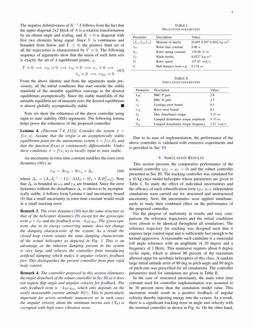
In the case of structured uncertainty, the main rotor timeconstant used for controller implementation was assumed tobe 30 percent more than the simulation model value. Thisincrement would result in a positive feedback of angularvelocity thereby injecting energy into the system. As a result,there is a significant tracking error in angle and velocity withthe nominal controller as shown in Fig. 4a. On the other hand,

9

-100

0

100Euler Angle (deg)

Ref roll Roll Pitch

-360

-180

0

180

360Angular Velocity (deg/s)

Ref x x y

-5

0

5Flap Angle (deg)

b a

0 0.5 1 1.5 2 2.5 3 3.5 4 4.5 5

Time (s)

-20

0

20

Cyclic Input (deg)

b a

(a) Nominal controller tracking response

-50

0

50

100Euler Angle (deg)

Ref roll Roll Pitch

-360

-180

0

180

360Angular Velocity (deg/s)

Ref x x y

-4

-2

0

2Flap Angle (deg)

b a

0 0.5 1 1.5 2 2.5 3 3.5 4 4.5 5

Time (s)

-10

0

10

Cyclic Input (deg)

b a r

(b) Robust controller tracking response

Fig. 4. Comparison of Robust and Nominal controller response for structured uncertainty

-50

0

50

100Euler Angle (deg)

Ref roll Roll Pitch

-360

-180

0

180

360Angular Velocity (deg/s)

Ref x x y

-5

0

5Flap Angle (deg)

b a

0 0.5 1 1.5 2 2.5 3 3.5 4 4.5 5

Time (s)

-10

0

10

Cyclic Input (deg)

b a

(a) Nominal controller tracking response

-50

0

50

100Euler Angle (deg)

Ref roll Roll Pitch

-360

-180

0

180

360Angular Velocity (deg/s)

Ref x x y

-5

0

5Flap Angle (deg)

b a

0 0.5 1 1.5 2 2.5 3 3.5 4 4.5 5

Time (s)

-10

0

10

Cyclic Input (deg)

b a r

(b) Robust controller tracking response

Fig. 5. Comparison of Robust and Nominal controller response for unstructured uncertainty

10

-100

0

100Euler Angle (deg)

Ref roll Roll Pitch

-360

-180

0

180

360Angular Velocity (deg/s)

Ref x x y

-5

0

5Flap Angle (deg)

b a

0 0.5 1 1.5 2 2.5 3 3.5 4 4.5 5

Time (s)

-20

0

20

Cyclic Input (deg)

b a

(a) Nominal controller tracking response

-50

0

50

100Euler Angle (deg)

Ref roll Roll Pitch

-360

-180

0

180

360Angular Velocity (deg/s)

Ref x x y

-5

0

5Flap Angle (deg)

b a

0 0.5 1 1.5 2 2.5 3 3.5 4 4.5 5

Time (s)

-10

0

10

Cyclic Input (deg)

b a r

(b) Robust controller tracking response

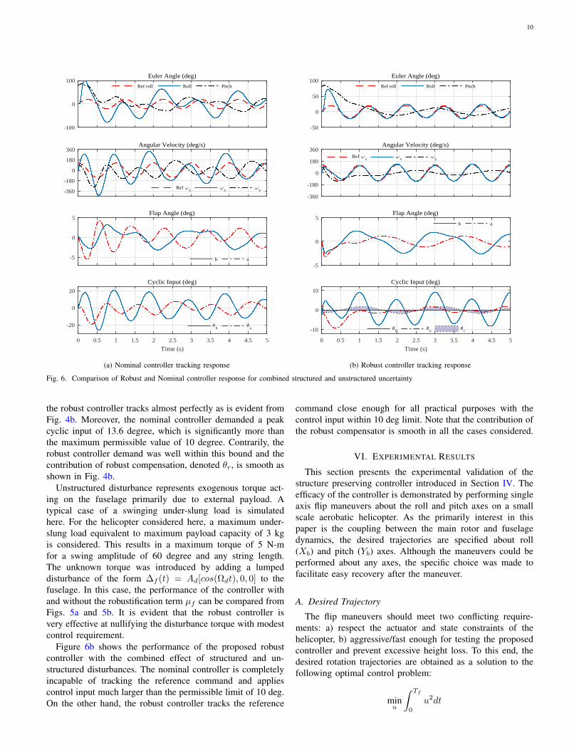
Fig. 6. Comparison of Robust and Nominal controller response for combined structured and unstructured uncertainty

the robust controller tracks almost perfectly as is evident fromFig. 4b. Moreover, the nominal controller demanded a peakcyclic input of 13.6 degree, which is significantly more thanthe maximum permissible value of 10 degree. Contrarily, therobust controller demand was well within this bound and thecontribution of robust compensation, denoted θr, is smooth asshown in Fig. 4b.

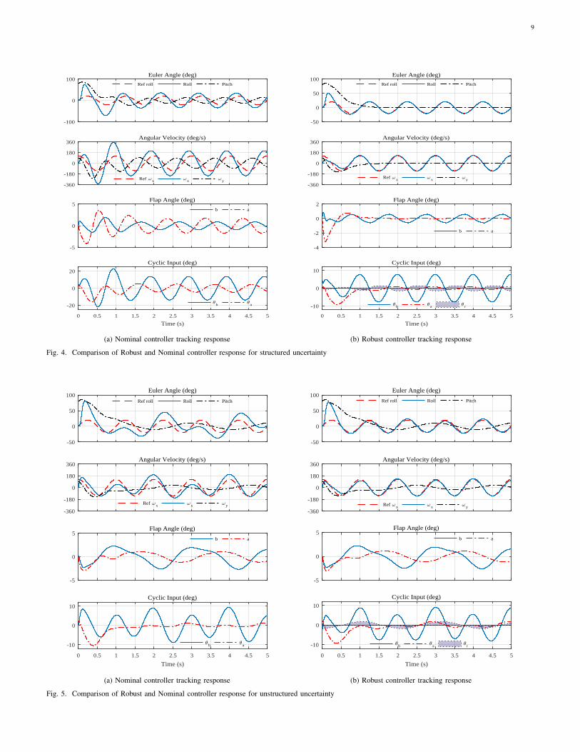
Unstructured disturbance represents exogenous torque act-ing on the fuselage primarily due to external payload. Atypical case of a swinging under-slung load is simulatedhere. For the helicopter considered here, a maximum under-slung load equivalent to maximum payload capacity of 3 kgis considered. This results in a maximum torque of 5 N-mfor a swing amplitude of 60 degree and any string length.The unknown torque was introduced by adding a lumpeddisturbance of the form ∆f (t) = Ad[cos(Ωdt), 0, 0] to thefuselage. In this case, the performance of the controller withand without the robustification term µf can be compared fromFigs. 5a and 5b. It is evident that the robust controller isvery effective at nullifying the disturbance torque with modestcontrol requirement.

Figure 6b shows the performance of the proposed robustcontroller with the combined effect of structured and un-structured disturbances. The nominal controller is completelyincapable of tracking the reference command and appliescontrol input much larger than the permissible limit of 10 deg.On the other hand, the robust controller tracks the reference

command close enough for all practical purposes with thecontrol input within 10 deg limit. Note that the contribution ofthe robust compensator is smooth in all the cases considered.

VI. EXPERIMENTAL RESULTS

This section presents the experimental validation of thestructure preserving controller introduced in Section IV. Theefficacy of the controller is demonstrated by performing singleaxis flip maneuvers about the roll and pitch axes on a smallscale aerobatic helicopter. As the primarily interest in thispaper is the coupling between the main rotor and fuselagedynamics, the desired trajectories are specified about roll(Xb) and pitch (Yb) axes. Although the maneuvers could beperformed about any axes, the specific choice was made tofacilitate easy recovery after the maneuver.

A. Desired Trajectory

The flip maneuvers should meet two conflicting require-ments: a) respect the actuator and state constraints of thehelicopter, b) aggressive/fast enough for testing the proposedcontroller and prevent excessive height loss. To this end, thedesired rotation trajectories are obtained as a solution to thefollowing optimal control problem:

minu

∫ Tf

0

u2dt

11

such that ω = φv,

Jω + ω × Jω = M,

M = AM −Kω +KAτθ,

θ = u

‖u‖ ≤ umax, ‖θ‖ ≤ θmax

∀t ∈ [0, Tf ]

(45)

with boundary conditions

φ(0) = 0, φ(Tf ) = φtr, ω(0) = 0, ω(Tf ) = 0,

M(0) = Mtr1 , M(Tf ) = Mtr2 ,

θ(0) = θtr1 , θ(Tf ) = θtr2

where (·)tr is the corresponding trim value for hover, u isthe rate of change of blade pitch input, and the attitude isdescribed by the axis-angle representation (φ, v)

Rd(φ, v) = I + sinφv + (1− cosφ)v2.

Since a single axis rotation is considered, v is a constantvector and the optimal attitude trajectory is obtained astime parametrized angle, φ(t). The proposed optimal controlproblem allows to include servo speed limit through umax,and ensure that the cyclic control input to the helicopter atthe beginning and end of the maneuver is its trim value.The maximum cyclic input, θmax, was set to 9.8 deg, whichcorresponds to a steady state angular velocity of 170 deg/sfor the given helicopter. A direct collocation method [33] wasused to obtain the optimal solution in Matlab.

B. Implementation Details

The experiments were carried out on Align Trex 700 electrichelicopter. It has a rotor diameter of 1.5 meter and weighs 6kg. The rotor rpm was set to 1500, although a higher rpmwould make the vehicle more capable of aerobatic flight. Itwas instrumented with Pixhawk autopilot board running amodified version of PX4 open source code. The board isequipped with a 3-axis accelerometer, 3-axis gyro and a 3-axis magnetometer together constituting the attitude headingreference system (AHRS). The stock code has an implementa-tion of quaternion based attitude estimator which fuses the datafrom the AHRS using a complementary filter. The controllerwas implemented as a separate module and runs at 250 Hz.Due to limited storage capacity of the autopilot ROM, theoptimal desired attitude trajectory was approximated usingpiecewise polynomials of degree 7 and 1, the coefficients ofwhich were stored onboard. Although, the SPR controller gainkR is a scaler in the theorem, for practical implementationit can be chosen to be a positive diagonal matrix to get thedesired handling quality about different axes. It can be chosenbased on the desired frequency characteristic of the linearizedstability matrix S(I) (41).

C. Experimental Results

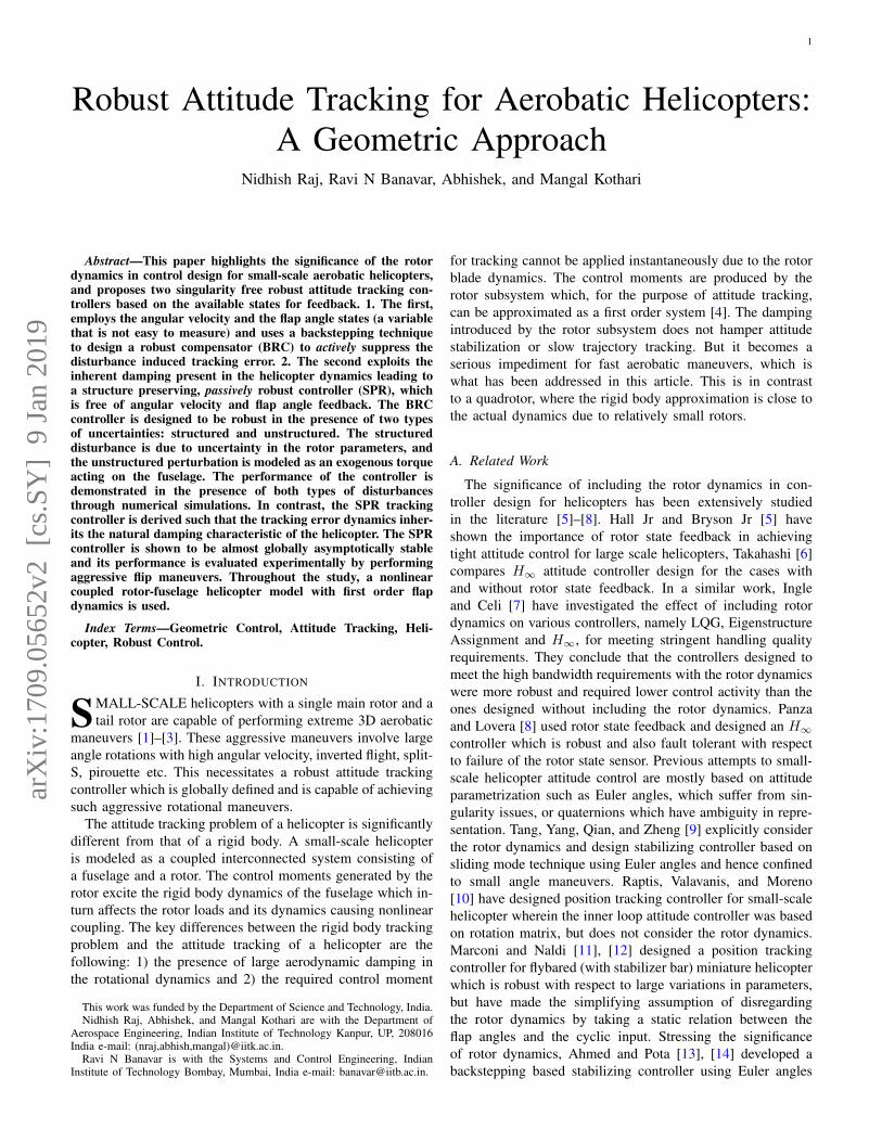
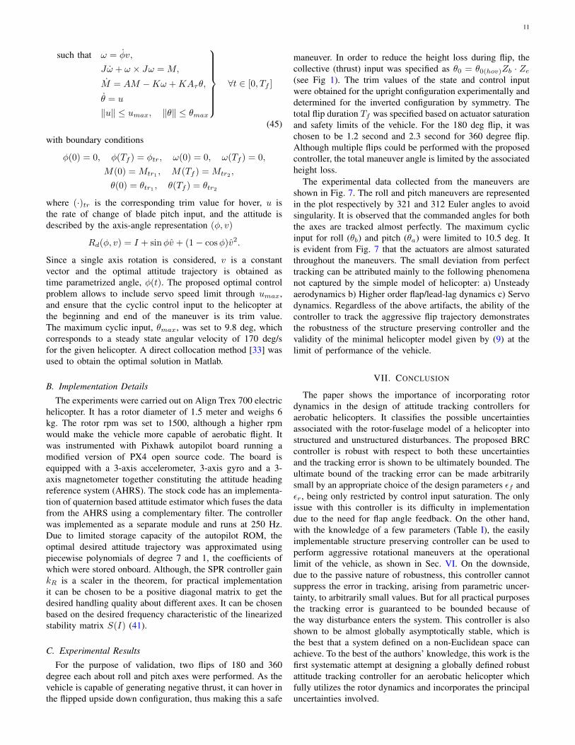
For the purpose of validation, two flips of 180 and 360degree each about roll and pitch axes were performed. As thevehicle is capable of generating negative thrust, it can hover inthe flipped upside down configuration, thus making this a safe

maneuver. In order to reduce the height loss during flip, thecollective (thrust) input was specified as θ0 = θ0(hov)Zb · Ze(see Fig 1). The trim values of the state and control inputwere obtained for the upright configuration experimentally anddetermined for the inverted configuration by symmetry. Thetotal flip duration Tf was specified based on actuator saturationand safety limits of the vehicle. For the 180 deg flip, it waschosen to be 1.2 second and 2.3 second for 360 degree flip.Although multiple flips could be performed with the proposedcontroller, the total maneuver angle is limited by the associatedheight loss.

The experimental data collected from the maneuvers areshown in Fig. 7. The roll and pitch maneuvers are representedin the plot respectively by 321 and 312 Euler angles to avoidsingularity. It is observed that the commanded angles for boththe axes are tracked almost perfectly. The maximum cyclicinput for roll (θb) and pitch (θa) were limited to 10.5 deg. Itis evident from Fig. 7 that the actuators are almost saturatedthroughout the maneuvers. The small deviation from perfecttracking can be attributed mainly to the following phenomenanot captured by the simple model of helicopter: a) Unsteadyaerodynamics b) Higher order flap/lead-lag dynamics c) Servodynamics. Regardless of the above artifacts, the ability of thecontroller to track the aggressive flip trajectory demonstratesthe robustness of the structure preserving controller and thevalidity of the minimal helicopter model given by (9) at thelimit of performance of the vehicle.

VII. CONCLUSION

The paper shows the importance of incorporating rotordynamics in the design of attitude tracking controllers foraerobatic helicopters. It classifies the possible uncertaintiesassociated with the rotor-fuselage model of a helicopter intostructured and unstructured disturbances. The proposed BRCcontroller is robust with respect to both these uncertaintiesand the tracking error is shown to be ultimately bounded. Theultimate bound of the tracking error can be made arbitrarilysmall by an appropriate choice of the design parameters εf andεr, being only restricted by control input saturation. The onlyissue with this controller is its difficulty in implementationdue to the need for flap angle feedback. On the other hand,with the knowledge of a few parameters (Table I), the easilyimplementable structure preserving controller can be used toperform aggressive rotational maneuvers at the operationallimit of the vehicle, as shown in Sec. VI. On the downside,due to the passive nature of robustness, this controller cannotsuppress the error in tracking, arising from parametric uncer-tainty, to arbitrarily small values. But for all practical purposesthe tracking error is guaranteed to be bounded because ofthe way disturbance enters the system. This controller is alsoshown to be almost globally asymptotically stable, which isthe best that a system defined on a non-Euclidean space canachieve. To the best of the authors’ knowledge, this work is thefirst systematic attempt at designing a globally defined robustattitude tracking controller for an aerobatic helicopter whichfully utilizes the rotor dynamics and incorporates the principaluncertainties involved.

12

0 0.2 0.4 0.6 0.8 1 1.2 1.4-200

-100

0

100321 Euler Angle (deg)

Ref roll Roll Pitch Yaw

0 0.2 0.4 0.6 0.8 1 1.2 1.4-300

-200

-100

0

100 (deg/s)

ref x x y z

0 0.2 0.4 0.6 0.8 1 1.2 1.4Time (s)

-15

-10

-5

0

5Cyclic Input (deg)

0 1c 1s

(a) Roll flip 180 deg

0 0.2 0.4 0.6 0.8 1 1.2 1.4-200

-100

0

100312 Euler Angle (deg)

ref pitch roll pitch yaw

0 0.2 0.4 0.6 0.8 1 1.2 1.4-300

-200

-100

0

100 (deg/s)

ref y x y z

0 0.2 0.4 0.6 0.8 1 1.2 1.4Time (s)

-15

-10

-5

0

5Cyclic Input (deg)

0 1c 1s

(b) Pitch flip 180 deg

0 0.5 1 1.5 2 2.5-400

-200

0

200321 Euler Angle (deg)

Ref roll Roll Pitch Yaw

0 0.5 1 1.5 2 2.5-300

-200

-100

0

100 (deg/s)

ref x x y z

0 0.5 1 1.5 2 2.5Time (s)

-15

-10

-5

0

5Cyclic Input (deg)

0 1c 1s

(c) Roll flip 360 deg

0 0.5 1 1.5 2 2.5-200

0

200

400312 Euler angle (deg)

ref pitch roll pitch yaw

0 0.5 1 1.5 2 2.5-100

0

100

200

300 (deg/s)

ref y x y z

0 0.5 1 1.5 2 2.5time (s)

-5

0

5

10

15Cyclic input (deg)

0 1c 1s

(d) Pitch flip 360 deg

Fig. 7. Experimental validation of the structure preserving controller by performing roll and pitch flip.

13

(a) Roll flip 180 deg (b) Pitch flip 180 deg

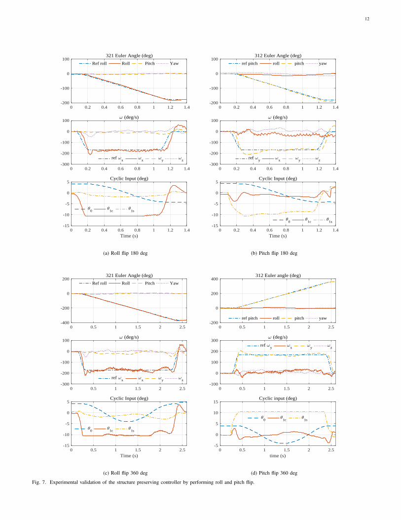
Fig. 8. Instants during the flip maneuver. Video link: https://youtu.be/1zz71W__RNA

APPENDIX ALINEARIZATION OF ERROR DYNAMICS

Proof. To linearize (40a), we first evaluate

d

dε

∣∣∣∣ε=0

R(ε) = Reqeε ˆη ˆη

∣∣∣∣ε=0

= Req ˆη. (46)

Linearization of (40a) is done by taking derivative of LHS andRHS w.r.t ε at ε = 0

d

dt

d

dε

∣∣∣∣ε=0

R(ε) =d

dε

∣∣∣∣ε=0

R(ε)ε ˆω (47)

which leads to

Req˙η = Req ˆω =⇒ ˙η = ω. (48)

Using the fact (Q−QT )∨ =∑3i=1 ei×Qei for all Q ∈ R3×3,

eRm = 12

∑3i=1 ei × PR(ε)ei. Thus

d

dε

∣∣∣∣ε=0

eRm =1

2

3∑i=1

eiPReq ˆηei = −1

2

3∑i=1

eiPReq eiη

= B(Req)η.

(49)

Using the above relation a similar procedure is followed tolinearize (40b) and (40c).

REFERENCES

[1] V. Gavrilets, E. Frazzoli, B. Mettler, M. Piedmonte, and E. Feron,“Aggressive maneuvering of small autonomous helicopters: A human-centered approach,” The International Journal of Robotics Research,vol. 20, no. 10, pp. 795–807, 2001.

[2] P. Abbeel, A. Coates, and A. Y. Ng, “Autonomous helicopter aerobaticsthrough apprenticeship learning,” The International Journal of RoboticsResearch, vol. 29, no. 13, pp. 1608–1639, 2010.

[3] M. B. Gerig, “Modeling, guidance, and control of aerobatic maneuversof an autonomous helicopter,” Ph.D. dissertation, ETH ZURICH, 2008.

[4] B. Mettler, Identification modeling and characteristics of miniaturerotorcraft. Springer Science & Business Media, 2013.

[5] W. Hall Jr and A. Bryson Jr, “Inclusion of rotor dynamics in controllerdesign for helicopters,” Journal of Aircraft, vol. 10, no. 4, pp. 200–206,1973.

[6] M. D. Takahashi, “H-infinity helicopter flight control law design withand without rotor state feedback,” Journal of Guidance, control, andDynamics, vol. 17, no. 6, pp. 1245–1251, 1994.

[7] S. J. Ingle and R. Celi, “Effects of higher order dynamics on helicopterflight control law design,” Journal of the American Helicopter Society,vol. 39, no. 3, pp. 12–23, 1994.

[8] S. Panza and M. Lovera, “Rotor state feedback in helicopter flightcontrol: robustness and fault tolerance,” in Control Applications (CCA),2014 IEEE Conference on. IEEE, 2014, pp. 451–456.

[9] S. Tang, Q. Yang, S. Qian, and Z. Zheng, “Attitude control of a small-scale helicopter based on backstepping,” Proceedings of the Institutionof Mechanical Engineers, Part G: Journal of Aerospace Engineering,vol. 229, no. 3, pp. 502–516, 2015.

[10] I. A. Raptis, K. P. Valavanis, and W. A. Moreno, “A novel nonlinearbackstepping controller design for helicopters using the rotation matrix,”IEEE Transactions on Control Systems Technology, vol. 19, no. 2, pp.465–473, 2011.

[11] L. Marconi and R. Naldi, “Robust nonlinear control for a miniaturehelicopter for aerobatic maneuvers,” in Proceedings 32nd RotorcraftForum, Maasctricht, The Netherlands, 2006, pp. 1–16.

14

[12] ——, “Robust full degree-of-freedom tracking control of a helicopter,”Automatica, vol. 43, no. 11, pp. 1909–1920, 2007.

[13] B. Ahmed and H. R. Pota, “Flight control of a rotary wing uav usingadaptive backstepping,” in Control and Automation, 2009. ICCA 2009.IEEE International Conference on. IEEE, 2009, pp. 1780–1785.

[14] B. Ahmed, H. R. Pota, and M. Garratt, “Flight control of a rotary winguav using backstepping,” International Journal of Robust and NonlinearControl, vol. 20, no. 6, pp. 639–658, 2010.

[15] B. Zhu and W. Huo, “Robust nonlinear control for a model-scaledhelicopter with parameter uncertainties,” Nonlinear Dynamics, vol. 73,no. 1-2, pp. 1139–1154, 2013.

[16] E. Frazzoli, M. A. Dahleh, and E. Feron, “Trajectory tracking controldesign for autonomous helicopters using a backstepping algorithm,” inAmerican Control Conference, 2000. Proceedings of the 2000, vol. 6.IEEE, 2000, pp. 4102–4107.

[17] N. Raj, R. N. Banavar, M. Kothari et al., “Attitude tracking control foraerobatic helicopters: A geometric approach,” in Decision and Control(CDC), 2017 IEEE 56th Annual Conference on. IEEE, 2017, pp. 1951–1956.

[18] R. T. Chen, “Effects of primary rotor parameters on flapping dynamics,”1980.

[19] F. Bullo and A. D. Lewis, Geometric control of mechanical systems:modeling, analysis, and design for simple mechanical control systems.Springer Science & Business Media, 2004, vol. 49.

[20] T. Lee, M. Leok, and N. H. McClamroch, “Nonlinear robust trackingcontrol of a quadrotor uav on se (3),” Asian Journal of Control, vol. 15,no. 2, pp. 391–408, 2013.

[21] D. S. Maithripala, J. M. Berg, and W. P. Dayawansa, “Almost-globaltracking of simple mechanical systems on a general class of lie groups,”IEEE Transactions on Automatic Control, vol. 51, no. 2, pp. 216–225,2006.

[22] T. Lee, “Robust Adaptive Geometric Tracking Controls on SO(3) withan Application to the Attitude Dynamics of a Quadrotor UAV,” ArXive-prints, Aug. 2011.

[23] H. Khalil, Nonlinear Systems, ser. Pearson Education. PrenticeHall, 2002. [Online]. Available: https://books.google.co.in/books?id=t_d1QgAACAAJ

[24] R. Kufeld, D. L. Balough, J. L. Cross, and K. F. Studebaker, “Flight test-ing the uh-60a airloads aircraft,” in ANNUAL FORUM PROCEEDINGS-AMERICAN HELICOPTER SOCIETY, vol. 5. American HelicopterSociety, 1994, pp. 557–557.

[25] R. Mahony, T. Hamel, and J.-M. Pflimlin, “Nonlinear complementaryfilters on the special orthogonal group,” IEEE Transactions on automaticcontrol, vol. 53, no. 5, pp. 1203–1218, 2008.

[26] D. E. Koditschek, “The application of total energy as a lyapunov functionfor mechanical control systems,” Contemporary mathematics, vol. 97, p.131, 1989.

[27] S. P. Bhat and D. S. Bernstein, “A topological obstruction to con-tinuous global stabilization of rotational motion and the unwindingphenomenon,” Systems & Control Letters, vol. 39, no. 1, pp. 63–70,2000.

[28] N. A. Chaturvedi, N. H. McClamroch, and D. S. Bernstein, “Asymptoticsmooth stabilization of the inverted 3-d pendulum,” IEEE Transactionson Automatic Control, vol. 54, no. 6, pp. 1204–1215, 2009.

[29] R. Bayadi and R. N. Banavar, “Almost global attitude stabilization of arigid body for both internal and external actuation schemes,” EuropeanJournal of Control, vol. 20, no. 1, pp. 45–54, 2014.

[30] D. Chillingworth, J. Marsden, and Y. Wan, “Symmetry and bifurcationin three-dimensional elasticity, part i,” Archive for Rational Mechanicsand Analysis, vol. 80, no. 4, pp. 295–331, 1982.

[31] J. Guckenheimer and P. Holmes, Nonlinear oscillations, dynamicalsystems, and bifurcations of vector fields. Springer Science & BusinessMedia, 2013, vol. 42.

[32] H. J. Marquez, Nonlinear control systems: analysis and design. Wiley-Interscience Hoboken, 2003, vol. 1.

[33] J. T. Betts, Practical methods for optimal control and estimation usingnonlinear programming. Siam, 2010, vol. 19.