Robust adaptive stabilization for time-varying systems with unmodelled dynamics and disturbances

INTERNATIONAL JOURNAL OF ADAFTIVE CONTROL AND SIGNAL PROCESSING, VOL. 10,531-550 (1996)

ROBUST ADAPTIVE STABILIZATION FOR TIME-VARYING SYSTEMS WITH UNMODELLED DYNAMICS AND

DISTURBANCES

YONG LI AND HAN-FU CHEN Institute of Systems Science, Academia Sinica. Beijing 1OOO80. People’s Republic of China

SUMMARY In this paper, robust adaptive stabilization is discussed for time-varying discrete time systems with disturbances and unmodelled dynamics. Both bounded and unbounded stochastic disturbances are considered. It is assumed that the parameters of the nominal model belong to a bounded convex set and that the ‘frozen time’ nominal model is stabilizable for all possible parameter values. Requiring neither external excitation nor stable invertibility of the nominal model. an adaptive regulator is constructed on the basis of the solution to a finite time Riccati equation and a projected gradient estimator. It is shown that the closed-loop system is stable if both the time average of the parameter variations and the model error are sufficiently small.

KEY WORDS adaptive control; robust stability; time-varying systems

1. INTRODUCTION

Since the beginning of the 1980s the robustness of adaptive control systems in the presence of disturbances and unmodelled dynamics has received much attention from adaptive control researchers (See, for example, References 1, 2). In most existing work, systems with model errors are adaptively stabilized for the case where the nominal plants are time-invariant. However, one of the motivations for adaptive control is to design controllers which perform satisfactorily for systems with time-varying parameters, so recently there has been a growing collection of results on robust adaptive controllers for time-varying systems.

When disturbances of a system are uniformly bounded, some interesting results are presented in Reference 3-9 under the assumption that the modelling errors are small and the parameters vary slowly. In Reference 3 de Larminat and Raynaud considered robustness properties for a fairly general indirect adaptive control law which uses two parallel estimators as well as a specially constructed ’normalization’ signal. Middleton and Goodwin4 also incorporated a normalization signal and additionally assumed that the constant factor by which it overbounds the unmodelled dynamics is known. They applied this constant to set up a normalized dead-zone for the algorithm and established robust stability of the system. Giri et aL5 by using an internally generated excitation, showed that a direct adaptive pole placement controller is robust with respect to plant parameter variation and modelling errors. Later they6 discussed the

CCC 0890-6327/96/06053 1-20 0 1995 by John Wiley & Sons, Ltd.

Received I5 August 1994 Revised I I June I995

532 Y. LI AND H.-F. CHEN

robustness of an adaptive regulator for a plant with small-in-the-mean parameter variations and unmodelled dynamics, using only the knowledge about the order of the nominal plant. However, some circulation in the argument of Reference 6 was pointed out by Zhang." Moreover, in the framework of Reference 6, arbitrarily large bounded disturbances cannot be handled and the regulation objective is not achieved even in the 'ideal' case. In Reference 7 Naik and Kumar showed that parameter projection in a gradient update law is sufficient for ensuring the boundedness of closed-loop signals for a nominally minimum phase time-varying discrete time plant with some type of unmodelled dynamics as well as bounded disturbances. Wen' established the robustness of an adaptive pole placement controller for time-varying discrete time systems by assuming that the 'frozen time' nominal model is controllable for all possible parameter values. Recently, for a discrete time plant with unmodelled dynamics and bounded disturbances, Jerbi et u Z . ~ constructed a robust adaptive regulator on the basis of the solution to a finite time Riccati equation and a projected parameter estimator with normalizing factor being chosen sufficiently large, assuming that the upper bound for disturbances is available.

Robustness of stochastic adaptive control systems with time-varying parameters has received comparatively less attention. Guo" established the stability of time-varying stochastic systems based on the projected gradient algorithm with small step size and analysed the robustness by using projection and normalization.

In this paper a robust adaptive regulator is constructed for time-varying discrete time systems with unmodelled dynamics and bounded or unbounded stochastic disturbances. In the case of bounded disturbance, similarly to Reference 9, we need no excitation signal and require no stable invertibility of the nominal model, but unlike Reference 9, we consider more general unmodelled dynamics and will not introduce any normalizing factor in the parameter estimator. Thus no upper bound of the disturbances is assumed to be available. It is shown that the input and output sequences of the closed-loop system are bounded (BIBO) if both the time average of the parameter variations and the model error are sufficiently small. For systems with unbounded stochastic disturbances, in comparison with Reference 1 1, robustness is established without requiring the nominally minimum phase condition. The closed-loop stability is proved on the basis of the Lp-exponential stability lemma for random linear equations which is given in Section 5.

To be precise, assume that the system is discrete time, single-input, single-output and time- varying:

i = 1 i = 1

where y(k), u ( k ) , ~ ( k ) and w ( k ) are the system output, input, uncertain dynamic error and disturbance respectively. The orders s and t of the nominal part of the system are assumed to be known. The initial conditions u( -1 ) ' ..., u ( - t ) , y(-1), . . . ,y ( - s) of the system are arbitrary and may be unknown. The coefficients a, (k) and b,(k) in (1) are unknown and time- varying.

Defining the parameter vector

o w = MQ, ..., a,(k) , b , ~ , ..., b,(k)iT

and the regressor vector

cp(k - 1) = [ y ( k - l), ..., y(k - s), u(k - l), .. ., u ( k - t ) lT

ROBUST ADAPTIVE STABILIZATION FOR TIME-VARYING SYSTEMS 533

we can rewrite (1) as

Y ( k ) = OT(k)q,(k- 1) + r ( k ) + w ( k ) (2)

Concerning ( l ) , we assume the following conditions.

A l . There exists a known, closed bounded convex subset D of R"' such that O(k) E D for all k .

A2. For any parameter vector 8 = [ O , , 02, ..., O,,,] E D the polynomials A ( z ) = zs - cs,l Oizs- i and B ( z ) = C:=, Os+iz'-' have no common zero in I z Ib 1.

A3. For some constant a B 0

A4.

or A3'. For some constant a' b 0

I r ( k ) I S a' II d k - 1) II (4) A4'. { w ( k ) , F , ] is an adapted sequence, with { F k } being a non-decreasing family of B-

algebra, and for some positive constants E and M,

E{exp[&l w ( k ) 1'1 IF , - , ] cexp(M,), as. , V k b O ( 5 )

It is worth noting that assumption A1 implies that there exist non-negative constants vo and v , such that

k - 1

x I I O ( i + l ) -O( i ) l l c v o + v , ( k - j ) , V k > j (6) i = j

The remainder of this paper is organized as follows. Section 2 introduces the parameter estimation algorithm and gives some preliminary results. Section 3 presents an adaptive controller based on the solution to a finite time Riccati equation, while Sections 4 and 5 give robust stability results of the systems with bounded disturbances and unbounded stochastic disturbances respectively. Finally, Section 6 gives some concluding remarks.

2. PARAMETER ESTIMATION AND PRELIMINARY RESULTS

The estimate for the unknown process O ( k ) is generated by the following projected version of the gradient algorithm:

with arbitrary initial condition &O) E D, where r> 0 is a constant to be specified later on and l l , ( x ) , denoting the projection from x to D, is defined as the point in D nearest to x (under the


Euclidean norm). We can readily prove that

llrID(e)- e,IlbJI 8 - eol), veEw+', e , m Define the output prediction error

e (k ) = y(k) - q T ( k - 1)&k - 1) = pT(k - i)[e(k) - &k - i ) ] + ~ ( k ) + ~ ( k )

e (k )

and the normalized output prediction error

F(k) = 4P + II d k - 1) 1l21

We can rewrite (7) in the form

e*(k) = &k - 1) + q ( k - i p ( k )

p ( k - 1) =

where p(k - 1)

4P + II v ( k - 1) 1l21

Lemma 1

For system (l), if assumptions A l , A3 and A4 hold with (3) and (6) satisfied and if there: exists a positive constant M I such that for some positive integer n

then max le(i)l c d + aM, + W I s i r n

where

Furthermore, if there exists a positive constant M such that for some positive integer t c n

Mb(1 q( i - l) l14Ml, r * i 4 n (15) then

I - I '1 P 2 ( i ) 4 u, + a2(k - j ) , n + 1 2 k > j 2 T i = j

where

M M


Proof. Set

8 ( k ) = 8 ( k - 1) - O ( k )

II Q(i> II c d

From (10) and (1 l), using (3) , (13) and the property that

for 1 s is n. we have

MI ; = j ; = j M

k- 1 k- I

e2(i) d 11 6( j ) - 11 6 ( k ) [ I 2 + 4 ( k - j ) + 4 Kj2( i ) + 2 d a - ( k -1)

c d 2 + [ 4( $[ + 2 d a 21 (k - j ) + 4 [ (:/ + d 51 ( k - j ) + (3d + 2 a 2) x [VcI + V l ( k -i l l

= a, + a 2 ( k - j )

Thus (17) is verified.

Applying the Schwarz inequality and using (17), we obtain the following corollary.

Corollary I

If the assumptions of Lemma 1 hold, then for n + 1 3 k > j P t

k - I c lC(i)l Q 4a,(k -j)I'' + 4a2(k - j ) i-j

0


- e , ( k ) ...... e s ( k ) e , + , ( k ) ...... o , + , ( k )

1

1 0 A ( N k ) ) = . . . . . . ...... 0 0 0 1

1 0

From (21), and by an argument similar to that used in the proof of Lemma 1, we can prove the following lemma.

(27)

Lemma I '

For system (1). if k > j a O

assumptions A l , A3' and A4' hold with (4) and (6) satisfied, then for all

k - I k - I 1 F ' ( i ) d b, + b2(k - j ) + 4 [S2( i ) + dl E(i) I] where

b, = d2 + 3dv0 + 2a'v0, b, = 4aI2 + 2da' + 3dv1 + 2a'v , (25)

3. CONSTRUCTION OF ADAPTIVE CONTROL LAW

The plant (1) can be represented in the state space form

d k ) = A(6(k ) ) (P(k - 1) + W k ) + g r l ( k ) + g w ( k ) where

Theorem I

Under assumption A2 there exists a row vector K ( 8 ) with entries from R ( 8 , , 8,. .... 6,+,) such that the eigenvalues of A (6) - bK( 6 ) are inside the disc of radius u, < 1 for 6 E D.

Consider the Riccati equation

P j + , ( 6 ) = I + AT ( 6 ) P j ( 0)A ( 6 ) - AT( 6 ) P j ( 6)b [ bTPj ( 6)b + h ] -IbTPj( 6)A ( 6 ) , j = 0, 1 .... (281

with initial condition Po = I, where h > 0 is a given real number. From results in References 9 and 12 under assumption A2 we can find a positive integer q and

0 < (T, < 1 such that the eigenvalues of A (6) - bK( 0) are inside the disc of radius (T, for all 6 E D, where

(29) K( 6 ) = [ b'P,( 6)b + h ] -'bTP,( 6 ) A ( 6 )


Using the row vector K( 8) defined by (29), we choose the adaptive control law as

u(k)= - K ( d ( k - l ) )q(k) (30) where 8 ( k - 1) is the estimate of 8 ( k - 1).

The control law (30) can be expressed as

where

K ( 8 ( k - 1)) = [d,(k) d,(k) ... d , ( k ) c , ( k ) C 2 ( k ) ... C f ( k ) I T

4. ROBUST STABILITY ANALYSIS FOR SYSTEMS WITH BOUNDED DISTURBANCES

We need the following lemma. For its proof we refer to Reference 13.

Lemma 2

Consider the linear time-varying system

~ ( k + 1) = [ A ( k ) + b(k)]x(k) and assume that for all k

11 A i ( k ) 11 d cBu,, V i > 0

and for all k > j k - 1 1 I I A < ~ + 1) - ~ ( i ) 11 s a, + a,(k - j f 2 + a,(k - j ) i = j

k - I c II b ( i ) II c P o + P l ( k -j)1'2 + B2(k --A i = j

where c,> 1, u, E (0,l) and a,, a , , a2, Po, Dl and p2 are positive constants. Furthermore, suppose that a2 and /I2 satisfy

a2 + P ~ / N < < ~ / d ' " - ga)/Nca

II ' Y ( k , j ) 1) ppk-'

where p E ( oa, 1) and N is a positive integer. Then for all k > j

where Y (k, j ) is the state transition matrix and

2 2 WI

p = (ca + x B r p - N sup La0 [cilN(ua + ca 1 i = O (Na i + Pi)(W)"-"'j/p] i = O

From (29) and assumption A1 we see that there exists a constant L>O such that for K(0) defined by (29)

11 K ( e ' ) - K ( 8 " ) L 11 8' - 8'' 11, ve', e E D (32)


From the boundedness of 0E D and the definition of K(8) in (29), we see that Z(8) is bounded by a positive constant W, and all its eigenvalues are inside the disc of radius oc < 1 for all 8 E D. Then, using results in Reference 14, we have

11 Z ( e > 11s cza;, for i = 1,2, ..., v& D (34) where

uc + 1 2S+'-'(l +o, +2w;+'-') az= -, c, =

2 (1 - oJ+'

Our first robust stability result is the following theorem.

Theorem 2

Under assumptions Al-A4 there exist real numbers vy > 0 and a* > 0 such that the closed- loop system consisting of parameter estimator (7), (8) with r = 1 and control law (30) is globally BIBO-stable provided that 0 d w1 S v: and 0 d a d a . *

Proof. Form (26) and (30) we see that the closed-loop system can be written in the state space

(35)

f o m

d k ) = tA(Nk)) - b f m k - 1 ) ) l d k - 1) + g r l ( k ) + g w ( k )

where A ( O ( k ) ) , K ( & k - 1)). b and g are as defined in Section 3. Using the relationship

where Z(.) is as defined in (33).

r = 1 we have We now express (37) in terms of the normalized output prediction error C ( k ) . From (11) and

Inserting (38) into (37) gives

where


Also, from (40) it follows that

Choosing pz = (0, + 1)/2

we can find a positive integer No satisfying

O < - - lU2 a, < 1 1lNo

cz

Denote c,[N0d(1 +L2) + I]

p2/c2 - 0 2 Wl,

i’ 1 /No

M* = 8(2 + d + 2W2+ 2dW)

d c z - u z

2c,“od(l + L Z ) + 11 v; =

(42)

(43)

(45)

(47) * 2 VO

a , = d +3dv0+2---;; M


From (44)- (49) we see M* > 1 and p: < 00.

Define

N , =min{Nisaninteger:p,*p;[(W,+d+ W + l ) M + ( d + W + l)] G M / 2 }

N,

MI = (W, + d + w + lP+h + (d + w + 1) c (W, + d + w + 1)’ j - 1

a* = 1 / M ,

and stopping times zi and oi: to = 0 and for any i 5 I

u ,=min{k>t , - , : 11 q ( k - 1)II>M]

zi = min( k > oi : 11 q ( k - 1) 11 s M ) * Clearly the assertion of the theorem will be verified if we can show that for 0s v, 6 v , and * OsaGa

SUP SUP II q ( k - 1111 d MI (56) i a l kE[o , , r , )

In fact, if

SUP I I q ( k - 1) I1 > MI (57) kE [ o , . r , )

then there is an integer k, defined by

k , = mini k E [o,, zl) , II q ( k - 1) II > MI I

II q ( k - 1) II 4 MI, V k € [O, k, - I ]

(58)

(5911

M<II v ( k - l ) l ldMl* V k € [ U l , k, - 11 (60)

Hence we have

Using Corollary 1, we obtain

k - I

( f?( i ) 1 s &,(k - j ) ” 2 + &,(k - j ) , k, S, k > j S, u1 (61) i=j

* * From the definitions of a: and a: we see that a , s a: and a,< a2 if O G v, G v, and 0s a d a*. From ( 4 3 , (46) and (48) it follows that

[d(l + L 2 ) + 1/No]Ja2 < (p2/c? - fJz)/Noc, (62)

By (42), (43), (61) and (62) and applying Lemma 2 to equation (39), we have

] ~ Y z ( k , j ) ~ ~ ~ p ~ ~ - ’ , Vk,- l a k > j a o l - 1

where Y2(k, j ) is the state transition matrix for (39), pz has been defined and p2 is a constant bounded by p: because of a, G a: and a2 C a:.

ROBUST ADAPTIVE STABILIZATION FOR TIME-VARYING SYSTEMS 54 1

From the definition of o1 we have

IIcP(ol-2)IlsM

11 q(ol - 1)11s ( W , + d + w + 1 ) M + (d+ w + 1)

which with (39) and (40) yields

Then, from (39) and by using Lemma 1, we derive

k , - 2 k"B-01 1 k - i - 2

s p z p z ( W , + d + W + l ) M + ( d + W + l ) + - d + - + - c pzp: M ( M i ) ; = u l - I

p,p:"-''(wz + d + w + l ) M + (d + w + 1) +

a p , p ~ - u l ( W , + d + W + 1 ) M + ( d + W + l ) + M / 2

which with (58) gives us

p*p>-"I(W,+ d + w + 1)M+ (d+ w + 1)>M/2

This and (51) imply

k, - a1 < N,

Thus, again from (39) and by using Lemma 1, we have k , - o , + 1

max IIZ(&i - 1)) + Q<i> 11 i c k , - 1

k , - 2 k,, - i - 2

+ ( max IlZ(&i - 1)) ; = o l - 2 i C k m - 1

k , - 2 k , - i - 2

Q ( W , + d + W + l f " - o l + l M + ( d + W + l ) c ( W , + d + W + l )

Q (W, + d + w + l p + l M + (d + w + 1) c (W, + d + w + 1)'

i - o l - 2

Nl

i - 0

= M ,

which contradicts (58). Therefore (57) is impossible, i.e.

542 Y. L1 AND H.-F. CHEN

Similarly to the argument used above, we obtain

SUP SUP I I d k - 1)II MI

SUP SUP IIq(k - 1111 6 MI

I c i 6 n + 1 k E (0,. r,)

provided that

I s i + n k € [ u , , r , )

Thus (56) is true and BIB0 stability follows.

5 . ROBUST STABILITY ANALYSIS FOR SYSTEMS WITH STOCHASTIC DISTURBANCES

We now give the Lp-exponential stability lemma for random linear equations.

Lemma 3

Consider the linear time-varying system

x ( k + 1) = [ A ( k ) + B ( k ) ] x ( k )

where A ( k ) and B ( k ) are random matrices satisfying for all k

11 A‘ (k ) 11 d c d , as . , t l i> 0 and for all k > j

E d exp[a, + a,(k - j ) ] , a s . i = j

where c> 1, a E (0,l) and a,, az, PI, p2 and M are positive constants. Furthermore, suppose that M, a, and #?* satisfy

M(l - 0 2 ) > 4 N ( N + 1)cZ

Bz M(1 -a2) 2P a 2 + - c N 2 N ( N + 1)c2 log( ~’/~(1 + 0’))

(72)

(73)

(74)

(75)

(76)

(77)

where

and N is a suitably large positive integer. Then for all k > j and 1 s p 6 M( 1 - 0 2 ) / 4 N ( N + 1)c2 [ E II Y(k, j ) l l P l l ’ P * f w k - j (78)

where Y(k , j ) is the state transition matrix of (72) and

(2Na, + 28, + N 2 a 2 + NB,)

ROBUST ADAITIVE STABILIZATION FOR TIME-VARYING SYSTEMS 543

Proof. Iterating (72) N times and using (73) gives us N - 1 I i - 0

I lx( t + N ) 11 = AN(t)x(t) + 1 A N - i - l ( f ) [ A ( t + i) - A ( t ) + B ( t + i ) ] x ( t + i)

N - 1

s caNII x ( t ) 11 + c ( J ~ - ~ - ’ //Act + i) - A ( t ) + B ( t + i) 11 I Ix(t + i) 11 (79) i = O

Setting 11 x ( t + i) 11 = a’z(t + i) and applying the Bellman-Gronwall inequality, we obtain N - I

z ( t + N) Q cz(t) + 1 5 IIA(t + i ) - A ( t ) + B ( t + i) I lz(t + i) i -0 a

C d cz(t); (1 + - ]]Act + i) - A ( t ) + B ( t + i)II

i - 0 (J

where

Iterating the inequality (82) n times gives n - 1 N - 1

I Ix( t + nN)(I’ 6 IIx(r){I’c” n n [al + c,l lA(t + j N + i) - A ( t + j N ) + B ( t + j N + i)II’] j = o i = o

Using the inequalities

and the fact that for 0 Q i d N - 1

1) A( t + j N + i ) - A( t + jN) + B( t + jN + i ) 11 ’


we derive

This implies

(84) For 1 s p s M( 1 - a 2 ) / 4 N ( N + 1)c2, using the Holder inequality and the fact that

MU: 8 2

N ( N + 1)pc:

from (74) and (75) we obtain

[Ell Y(t + nN, t ) I l p ] l / p


From (77) we have

which with (85) yields

For n N d k - j s (n+ l)N- 1 we have

[ E [ ( Y ( k , j ) ( I P I I / p G [ E ( ( Y ( k , j + n N ) l l p l l ~ o ’ + ~ ~ J ) I l p l l ~ p d [ E I I Y ( k , j + nlv)II 2’]1/2p[E)p0.+nN,j)II 2p11/2p (87)

Similarly to the argument used above, we obtain

Thus from (87)-(89) we have

and (78) follows.

We also need the following lemma cited from Reference 11.

Lemma 4

Let w be a random variable and F a o-algebra. If

E (eW21F}ded , as., forsomed>O

0


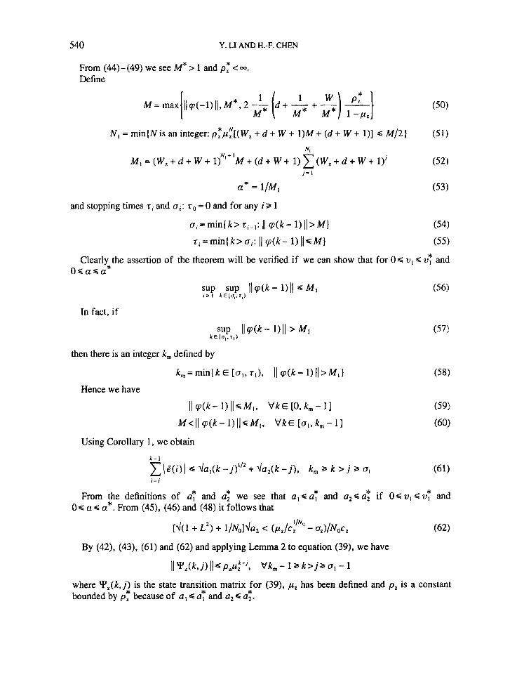
then for any real number a > 0

E { e"l w I 1 F ] Gexp{ ud1I2 + [i + 4a2(1 + e8"')]d), as. (92)

For systems with stochastic disturbances satisfying assumption A4', we have the following robust stability result.

Theorem 3

For plant (1) suppose that assumptions Al, A2, A3' and A4' hold and that in the estimation algorithm (7), (8) r is sufficiently large such that

(93) for some p, E (4 [ (1 + 0:)/2], 1) and the positive integers N and M are large enough such that

M(1-0:) > 1, > 23 w &".([(1 + 03/21 N(N + 1)c:

(94)

* Then there exist real numbers vT > 0 and a* > 0 such that if 0 c vi G v: and 0 G a' s a under the adapt.ive law (30), the closed-loop system is stable in the sense that

Proof. From (35)-(37) we see that the closed-loop system can be written in the state space

(96)

form

q ( k ) = ~ ( & k - l))q(k - 1) + g e ( k )

where Z ( . ) is as defined in (33) and g is as defined in Section 3. From (1 1) we have

From the definitions of Z ( - ) , el(.) and qi( . ) we see that ( Z ( & k - l ) ) ,Fk- ,} , ( Q , ( k ) , F , ] and { qi (k), Fk 1 are adapted sequences.


By an argument similar to that used in the proof of Theorem 2, we obtain k - 1 k - 1

11 Z ( 8 ( i ) ) - Z(&i - 1)) 11 d J(1 + L2) c I @(i) I, as., V k > j (loo) i=j i-j

k - I k - 1

C((Q,(i)Il c(W(, a-s., vk>j (101) i=j i-j

where L is the constant defined in (32). From (100) and the fact that

8M( 1 + L’) 8M( 1 + L 2 ) < < 1

re J(W using the Holder inequality and Lemma 1’, for M satisfying (94), we have

k- 1

Q exp(M(1 + L2)[bl + &(k - j ) ] ) E

Q exp(M(1 +L2) [b l

w2(i) + 2 Iw(i) I]} Jr

d w2(k- I ) + - Iw(k- 1)1

Jr d k - 2 1

+ L z ) c ( - i-j r w’(i)+ - Jr iw(i) l ) ]}


c exp(M(1 + Lz)[b, + &(k -;)I} 4M(1+ L 2 )

drE ( d d M w + [f + 4d2(1 + ew') ]Mw} M W +

where for the last inequality Lemma 4 is invoked. Repeating this argument k - j times yields

4M(1 + L 2 ) r&

+ L2)[b, + b2(k -;)I + Mw(k -;>

4M(1 + L 2 ) + { d d M , + [i + 4d2(1 + eM2)] M,)(k -;) Jh)

4M, 4 b3 = - + - {ddMw + [f + 4d2(1 + ewz)] M,)

re J(n) Similarly, from (101) we obtain

For N satisfying (94) and ,uz E ('J[(1 + 0,2)/2], I ) , from (93) we see

From (25) and (105) we see that there exist real numbers VT > 0 and a* > 0 such that

* where 09 v , d VT and 0s a' s a . Then, applying Lemma 3 to system (96) for 1 C J I c M(l - 03/4N(N + 1)c:, we obtain

[ E I1 Y&.i) I I p l l / p ~ P,P? (107)


where Y p ( k , j ) is the state transition matrix of (96), i.e. k

yp(kj) = n [z(e(i - 1)) + Ql(i>l

(107) and the Minkowski inequality, we

i = 1

k

i = 1

From the definition of q1 ( k ) , by Lemma 1’ we see

(109) From this and the fact that under assumption A4’ ( w ( k ) ] satisfies

2m 1/2m SUP { [ ~ j w ( k ) I 1 1 < m, ~ l m = 1,2 , ... k z O

using the Minkowski inequality, we derive 28 1/28 ;UP “q)41(k))) 1 1 < O0

P O

with which (108) implies

Thus from (2), (30), (112) and assumptions A l , A3‘ and A4‘ we obtain

6. CONCLUDING REMARKS

In this paper, for the single-input/single-output discrete time system modelled by a linear time- varying difference equation with disturbances and modelling errors, a robust adaptive stabilizing regulator is designed for the case where the model errors and the average parameter variations are sufficiently small and the disturbance is a random process.

For the projected least squares type of algorithm with data normalization and adaptation gain reinitialization, results similar to Theorems 2 and 3 can also be derived.

Further work of interest is to remove the condition that the nominal model is stabilizable for


all possible parameter values at ‘frozen time’, to delete the projection used in the algorithm and to enlarge the class of unmodelled dynamics for time-varying stochastic systems.

REFERENCES

1. Egardt, B., Stability of Adaptive Controllers. Springer, Berlin, 1979. 2. Ioannou, P. A. and J. Sun, ‘Theory and design of robust direct and indirect adaptive control schemes’, f n t . J.

Control, 47,775-813 (1988). 3. de Larminate, P. and H. Raynaud, ‘A robust solution to the admissibility problem in indirect adaptive control

without persistency of excitation’, Inr. j. adapt. control signal process., 2. 159-155 (1988). 4. Middleton, R. H. and G. C. Goodwin, ‘Adaptive control of time-varying linear systems’, IEEE Trans. Automatic

Control, AC-33, 150-155 (1988). 5. Gin, F., M. M’Saad, J. M. Dion and L. Dugard. ‘Pole placement direct adaptive control for time-varying ill-

modeled plant’, IEEE Trans. Automatic Control, AC-35.723-726 (1990). 6. Gin, F., M. M’Saad, L. Dugard and J. M. Dion, ‘Robust adaptive regulation with minimal pnori knowledge’,

IEEE Trans. Automatic Control, AC-37,305-315 (1992). 7. Naik, S. M. and P. R. Kumar, ‘Robust indirect adaptive control of time-varying plants with unmodeled dynamics

and disturbances’, SIAM J . Control Optimization, 32, 1696-1725 (1994). 8. Wen, C., ‘A robust adaptive controller with minimal modification for discrete time varying systems adaptive

control just using parameter projection’, Proc. 31st CDC, Tuscon. AZ, 1992, IEEE, New York, 2132-2136 1992.

9. Jerbi, A., E. W. Kamen and J. F. Dorsey, ‘Construction of a robust adaptive regulator for time-varying discrete time systems’, Int. j . adapt. control signalprocess., 7, 1-12 (1993).

10. Zhang, J. F.. ‘Comments on “Robust adaptive regulation with minimal prior knowledge” ’, IEEE Trans, Aufornalic Control, AC-39,605 (1994).

11. Guo, L., ‘On adaptive stabilization of time-varying stochastic systems’, SIAM J . Control Optim., 28, 1432---1451

12. Kamen, E. W. and P. P. Khargonekar. ‘On the control of linear system whose coefficients are functions of

13. Kreisselmeier. G., ‘Adaptive control of a class of slowly time-varying plants’, Syst. Control Lett., 8, 97-103

14. Desoer, A. C., ‘Slowing varying discrete system x i + , = Axi’, Electron. Lett., 6 , 339-340 (1970).

(1990).

parameters’, IEEE Trans. Automatic Control, AC-29,25-33 (1984).

(1986).

Documents

Robust adaptive stabilization for time-varying systems with unmodelled dynamics and disturbances