Embed Size (px)
Citation preview

Robotic Manipulation and Characterization of Cells for Drug Screen and Clinical IVF Applications
by
Jun Liu
A thesis submitted in conformity with the requirements for the degree of Doctor of Philosophy
Department of Mechanical and Industrial Engineering University of Toronto
© Copyright by Jun Liu 2016
ii
Robotic Manipulation and Characterization of Cells for Drug
Screen and Clinical IVF Applications
Jun Liu
Doctor of Philosophy
Department of Mechanical and Industrial Engineering
University of Toronto
2016
Abstract
Heterogeneity is the hallmark of cell biology. Robotic system and automated methods are
required for characterization and manipulation of a large number of single cells for many
important applications, such as characterizing cell-cell communication for screening drug effects,
processing oocytes or embryos for cryopreservation, and analyzing sperm locomotion behavior
for selection of a high-quality sperm for in vitro fertilization (IVF). However, current robotic
characterization and manipulation systems have two major limitations in search-and-locating
end-effector tips and determination of relative Z position between end-effector tips and single
cells. This research has addressed these two limitations by developing an auto-locating end-
effector tip method and two vision-based contact detection algorithms. By integrating the two
new solutions, I have built two robotic system prototypes for microinjection of a large number of
adherent cells and automatically processing oocytes or embryos for vitrification. The robotic
microinjection system enabled automated gap junction measurement for repurposing
antiarrhythmic drugs to identify optimal treatments for cardiac arrhythmias by assessing each
drug‟s efficacy on rescuing/enhancing gap junctions. Robotic vitrification relieves human
operators from tedious and difficult manual steps, eliminating operator errors and
inconsistencies. It also offers unparalleled timing control based on real-time embryo volume
iii
monitoring. Automation enables the system to process multiple oocytes/embryos with high
efficiency. In addition, automated methods were developed to quantitatively analyze sperm
locomotion behaviors by tracking both sperm head and tail. Experimental results on automated
sperm analysis revealed a significant correlation between sperm head velocity and tail beating
amplitude. By combining automated sperm motility analysis with DNA assessment technique,
this research offers a new solution for identifying single sperms of high quality for IVF
applications. In the end, this research also reviewed future research directions in microsystems
and nanoengineering for intracellular measurement and manipulations and discussed the
promising research for the intracellular study.

iv
Acknowledgments
It has been a relatively long journey since I first came to UofT in 2011. I feel very lucky and
grateful to have a great supervisor, Professor Yu Sun, who guided me through this exploration.
At first, I would like to sincerely thank Prof. Sun for his continuously strong support in my
study, research, personal life and career development. Professor Sun is a wonderful advisor, a
great writer, and a visionary leader. Without his guidance and support, I would not be able to
manage through this tough journey to push the boundary of knowledge for my Ph.D. degree.
Secondly, I want to thank Professor Goldie Nejat, Professor Lidan You, Dr. Jason Maynes and
Professor Jason Gu for serving on my Ph.D. supervisory and defense committees. Their
insightful comments and suggestions are critical for my Ph.D. research. I really appreciate their
time and support in helping me through the completion of my thesis.
Thirdly, I would like to thank all my talented and happy-to-be-around lab colleagues, who
offered generous help in designing research projects, conducting experiments, and drafting paper
manuscripts. Among all my lab colleagues, I should especially thank Zhe Lu and Clement, who
taught me at the very beginning of my study in AMNL. Also, I would like to give my special
thanks to Brandon, Yanliang, Yong Zhang, and Yi Zheng, who provide generous help at the
beginning and throughout my time in AMNL. In addition, I enjoyed working and laughing with
Haijiao, Jun Wen, and Zhuoran. You guys know me. Also, I want to thank Derek, John, Yuan,
Wes, and Devin, who shared with me a lot intercultural funny stuff.
Especially, I want to express my appreciation to all my collaborators, especially Dr. Robert
Hamilton, Dr. Jason Maynes, and Dr. Sevan Hopyan. Their valuable knowledge and insightful
suggestions inspired me to design research projects, conduct experiments and understand results.
It is you doctors who provided such great collaboration opportunities for me to realize my true
value of being an engineer to contribute to our society.
In the end, I would like to thank my parents and my two beloved sisters, who always stand
behind me to support. Lastly but most importantly, I want to thank my dear wife, Qiaorong Fan.
Without her understanding, support, love, and care for our family, I would not be able to travel
this far. My entire Ph.D. work is incomparable to your great achievements of two angels – Alan
and Daniel. It is your endless love that brings me true happiness.

v
Contribution of Co-authors
I am the principle or co-principle author of all the articles on which this thesis is partially based.
I have performed all or the majority of experiments, data collection, analysis, and manuscript
preparation for each article. I would like to acknowledge all of my co-authors for their valuable
contributions. Also, I acknowledge my supervisor, Professor Yu Sun, who provided knowledge,
ideas and directions that were critical in my entire research and he was involved in manuscript
preparation for each article presented here. The following outlines the contributions of each co-
author:
[1] J. Liu, Z. Gong, K. Tang, Z. Lu, C. Ru, J. Luo, S. Xie, and Y. Sun, "Locating end-effector
tips in robotic micromanipulation," IEEE Transactions on Robotics, Vol. 30, pp. 125-30,
2014.
Professor Y. Sun was involved in project design and manuscript preparation. Discussions
regarding research concepts, collection and interpretation of data were continuously
conducted among all contributing authors.
[2] J. Liu, V. Siragam, Z. Gong, J. Chen, M.D. Fridman, C. Leung, Z. Lu, C.H. Ru, S.R. Xie, J.
Luo, R. Hamilton, and Y. Sun, "Robotic adherent cell injection (RACI) for characterizing
cell-cell communication," IEEE Transactions on Biomedical Engineering, vol. 62, no. 1, pp.
119-24, 2015.
Professor Y. Sun and Dr. R. Hamilton were involved in project design and manuscript
preparation. V. Siragam was involved in cell preparation and data interpretation. Z. Gong, J.
Chen, C. Leung, and Z. Lu helped in building the system hardware and programming
software. Discussions regarding research concepts, collection and interpretation of data were
continuously conducted among all contributing authors.
[3] J. Liu, V. Siragam, J. Chen, M.D. Fridman, R.M. Hamilton, and Y. Sun, "High-throughput
measurement of gap junctional intercellular communication," American Journal of
Physiology - Heart and Circulatory Physiology (AJP-Heart), Vol. 306, pp. H1708-13, 2014.
Professor Y. Sun and Dr. R. Hamilton were involved in project design and manuscript
preparation. V. Siragam and M. Fridman were involved in cell preparation and data
vi
interpretation. Discussions regarding research concepts, collection and interpretation of data
were continuously conducted among all contributing authors.
[4] J. Liu, C.Y. Shi, J. Wen, D.G. Pyne, H.J. Liu, C.H. Ru, S.R. Xie, Y. Sun, “Automated
Robotic Vitrification of Embryos,” Robotics & Automation Magazine, vol. 22, pp. 33-40,
2015.
Professor Y. Sun was involved in project design and manuscript preparation. Discussions
regarding research concepts, collection and interpretation of data were continuously
conducted among all contributing authors.
[5] J. Liu, C. Leung, Z. Lu, and Y. Sun, "Quantitative analysis of locomotive behavior of
human sperm head and tail," IEEE Transactions on Biomedical Engineering, Vol. 60, pp.
390-396, 2013.
Professor Y. Sun and Z. Lu were involved in project design and manuscript preparation.
Discussions regarding research concepts, collection and interpretation of data were
continuously conducted among all contributing authors.
[6] J. Liu, C. Moraes, Z. Lu, C.A. Simmons, and Y. Sun, "Single cell deposition," Methods in
Cell Biology, Vol. 112, pp. 403-420, 2012.
Professor Y. Sun and C.A. Simmons were involved in designing the project. All authors
were involved in manuscript preparation.
[7] J. Liu, J. Wen, Z.R. Zhang, H.J. Liu, and Y. Sun, “Voyage inside the Cell: Microsystems
and Nanoengineering for Intracellular Manipulation and Characterization”, Microsystem &
Nanoengineering, vol. 1, p. 15020, 2015.
Professor Y. Sun designed the project and all authors are involved in manuscript preparation.
Discussions regarding research concepts and literature reviews were continuously conducted
among all contributing authors.

vii
To Qiaorong Fan, my dear and loving wife

viii
Table of Contents
Acknowledgments.......................................................................................................................... iv
Contribution of Co-authors ..............................................................................................................v
Table of Contents ......................................................................................................................... viii
List of Tables ................................................................................................................................ xii
List of Figures .............................................................................................................................. xiii
Chapter 1 Introduction .....................................................................................................................1
Introduction .................................................................................................................................1 1
1.1 Single Cell Characterization and Manipulation ...................................................................1
1.2 Characterization of Gap Junctional Intercellular Communication ......................................4
1.3 Robotics and Automation for in vitro Fertilization..............................................................6
1.3.1 Robotic Vitrification of Mammalian Embryos ........................................................6
1.3.2 Quantitative Analysis of Sperm Locomotion Behavior ...........................................8
1.4 Previous Methods for Robotic Cell Manipulation .............................................................10
1.5 Opportunities for Innovations in Robotic Cell Manipulation ............................................16
1.6 Research Objectives ...........................................................................................................17
1.7 Dissertation Outline ...........................................................................................................18
Chapter 2 Automatically Locating End-effector Tips in Micromanipulation ...............................19
Automatically Locating End-Effector Tips in Micromanipulation ...........................................20 2
2.1 Introduction ........................................................................................................................21
2.2 System Design ...................................................................................................................23
2.2.1 System Architecture ...............................................................................................23
2.2.2 Overall Sequence ...................................................................................................24
2.3 Key Methods for Auto-Locating End-effector Tips ..........................................................25
2.3.1 End-Effector Sweep Pattern Design ......................................................................25

ix
2.3.2 Computer Vision Based End-Effector Detection ...................................................26
2.3.3 Detection of End-Effector Contours ......................................................................27
2.3.4 Autofocusing on End-Effector Tips .......................................................................28
2.3.5 Centering End-Effector Tips via Visual Servo Control .........................................30
2.4 Experimental Results and Discussion ................................................................................31
2.4.1 Overall Performance ..............................................................................................31
2.4.2 Performance Under Different Microscopy Imaging Modes ..................................32
2.4.3 Discussion ..............................................................................................................35
2.5 Conclusion and Guidelines for Implementation ................................................................37
Chapter 3 Robotic Microinjection of Adherent Cells ....................................................................38
Robotic Microinjection of Adherent Cells ................................................................................39 3
3.1 Introduction ........................................................................................................................39
3.2 System Setup ......................................................................................................................42
3.3 Vision Based Contact Detection ........................................................................................44
3.3.1 Contact Detection on Cell Culture Surface ............................................................44
3.3.2 Contact Detection on Cell Membrane....................................................................45
3.4 Robotic Microinjection ......................................................................................................49
3.5 Experimental Results and Discussion ................................................................................51
3.5.1 Performance of Locating Micropipette Tip ...........................................................51
3.5.2 Injection Speed.......................................................................................................51
3.5.3 Injection Success Rate and Cell Survival Rate ......................................................52
3.5.4 Characterization of Cell-Cell Communication ......................................................53
3.5.5 Discussion ..............................................................................................................56
3.6 Conclusion .........................................................................................................................56
Chapter 4 Robotic Vitrification of Mammalian Embryos .............................................................57
Robotic Vitrification of Mammalian Embryos .........................................................................58 4

x
4.1 Cryopreservation of Oocytes and Embryos .......................................................................58
4.2 System Overview ...............................................................................................................61
4.3 Key Methods for Robotic Vitrification ..............................................................................63
4.3.1 Contact Detection...................................................................................................63
4.3.2 Embryo Tracking in Three-Dimensional Space ....................................................64
4.3.3 Placing Embryo on Vitrification Straw ..................................................................68
4.4 Results and Discussion ......................................................................................................70
4.4.1 System Performance ..............................................................................................70
4.4.2 Embryo Volume Measurement ..............................................................................71
4.4.3 Post-Freezing Survival and Development Rates....................................................73
4.4.4 Discussion ..............................................................................................................74
4.5 Conclusion .........................................................................................................................75
Chapter 5 Automated Analysis of Sperm Locomotion Behavior ..................................................76
Automated Analysis of Sperm Locomotion Behavior ..............................................................77 5
5.1 Introduction ........................................................................................................................77
5.2 System Setup and Experimental Design ............................................................................80
5.3 Computer Vision Methods for Sperm Tracking ................................................................81
5.3.1 Overview ................................................................................................................81
5.3.2 Sperm Head Tracking ............................................................................................82
5.3.3 Sperm Tail Tracking ..............................................................................................85
5.4 Experimental Results and Discussion ................................................................................88
5.5 Conclusion .........................................................................................................................93
Chapter 6 Conclusions and Future Research .................................................................................94
Conclusions and Future Research .............................................................................................94 6
6.1 Contributions......................................................................................................................94
6.2 Future Research .................................................................................................................95

xi
6.2.1 Improvement of the Present Research ...................................................................95
6.2.2 Research Outlooks on Intracellular Measurement and Manipulations ..................97
References ....................................................................................................................................100

xii
List of Tables
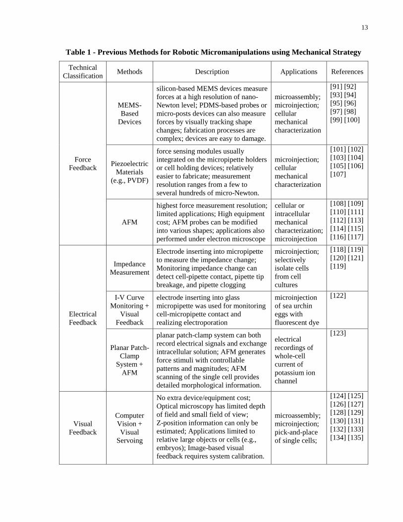
Table 1 - Previous Methods for Robotic Micromanipulations using Mechanical Strategy .......... 13
Table 2 - Experiment Results of Auto-Locating End-Effector Tips Under Three Different
Microscopy Imaging Modes ......................................................................................................... 33
Table 3 - Effect of Different Threshold Values on Detection Time and Overall Success Rate
(Each Data Point in the Table Was from 100 Trials, All Under Bight Field Imaging) ................ 35
Table 4 - Robotic Microinjection Speed of Three Different Cell Lines ....................................... 51
Table 5 - Injection Success Rate and Cell Survival Rate After Injection ..................................... 52
Table 6 - Embryo Vitrification Experimental Results .................................................................. 71
Table 7 - Dynamic Representation of Sperm Positions in Multi-Sperm Tracking Algorithm ..... 83
Table 8 - Performance Comparison Between MHI-Based Multi-Sperm Tracking and GNN-Based
Multi-Sperm Tracking .................................................................................................................. 88
Table 9 - Average Tracking Error of Sperm Tail Tracking .......................................................... 89
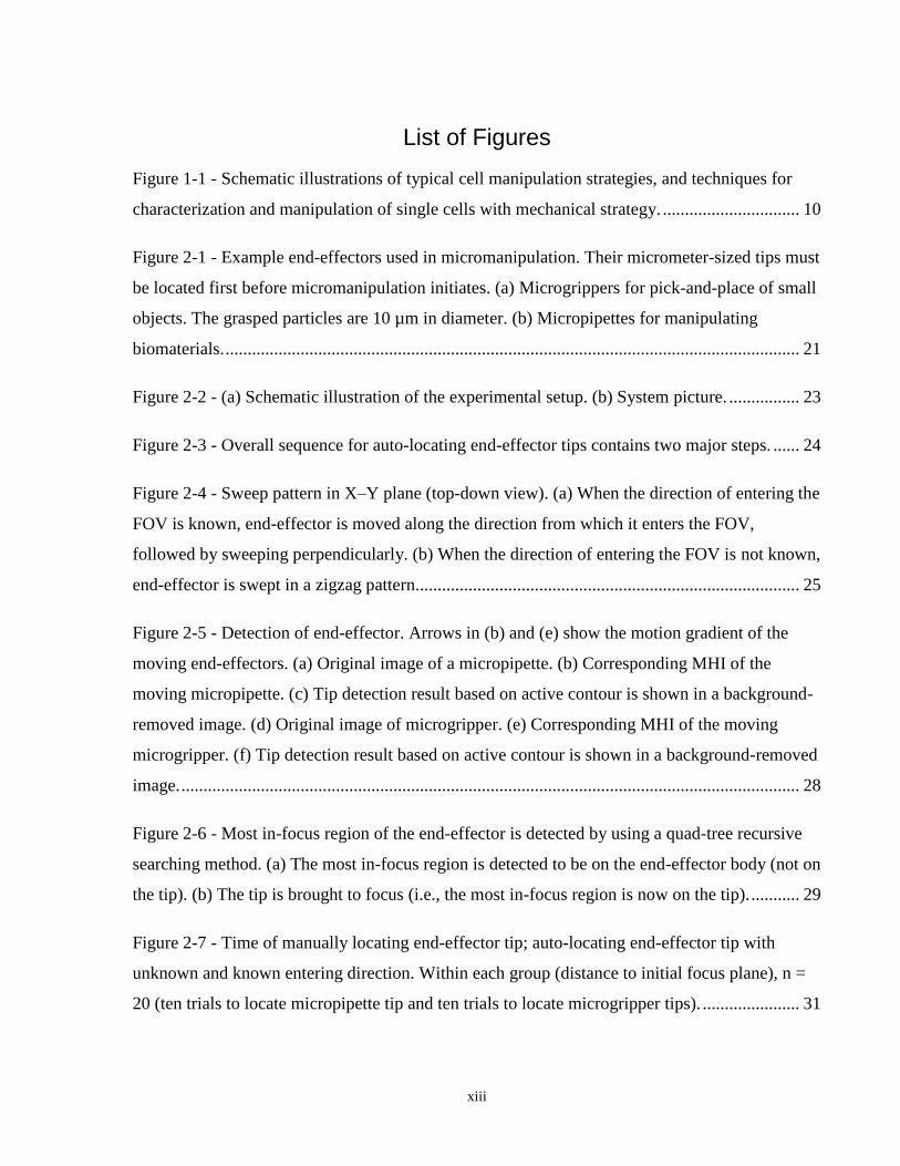
xiii
List of Figures
Figure 1-1 - Schematic illustrations of typical cell manipulation strategies, and techniques for
characterization and manipulation of single cells with mechanical strategy. ............................... 10
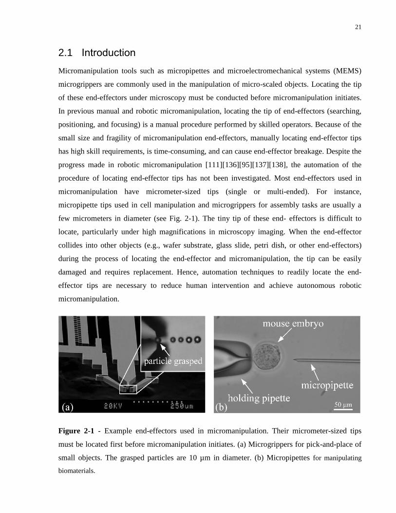
Figure 2-1 - Example end-effectors used in micromanipulation. Their micrometer-sized tips must
be located first before micromanipulation initiates. (a) Microgrippers for pick-and-place of small
objects. The grasped particles are 10 µm in diameter. (b) Micropipettes for manipulating
biomaterials. .................................................................................................................................. 21
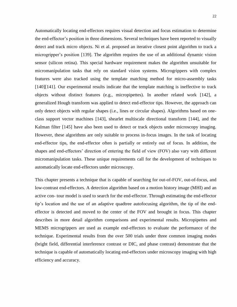
Figure 2-2 - (a) Schematic illustration of the experimental setup. (b) System picture. ................ 23
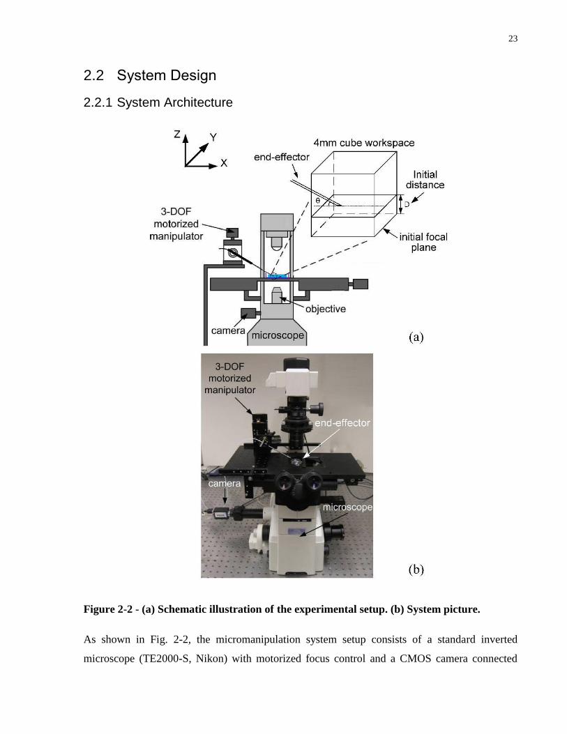
Figure 2-3 - Overall sequence for auto-locating end-effector tips contains two major steps. ...... 24
Figure 2-4 - Sweep pattern in X–Y plane (top-down view). (a) When the direction of entering the
FOV is known, end-effector is moved along the direction from which it enters the FOV,
followed by sweeping perpendicularly. (b) When the direction of entering the FOV is not known,
end-effector is swept in a zigzag pattern....................................................................................... 25
Figure 2-5 - Detection of end-effector. Arrows in (b) and (e) show the motion gradient of the
moving end-effectors. (a) Original image of a micropipette. (b) Corresponding MHI of the
moving micropipette. (c) Tip detection result based on active contour is shown in a background-
removed image. (d) Original image of microgripper. (e) Corresponding MHI of the moving
microgripper. (f) Tip detection result based on active contour is shown in a background-removed
image. ............................................................................................................................................ 28
Figure 2-6 - Most in-focus region of the end-effector is detected by using a quad-tree recursive
searching method. (a) The most in-focus region is detected to be on the end-effector body (not on
the tip). (b) The tip is brought to focus (i.e., the most in-focus region is now on the tip). ........... 29
Figure 2-7 - Time of manually locating end-effector tip; auto-locating end-effector tip with
unknown and known entering direction. Within each group (distance to initial focus plane), n =
20 (ten trials to locate micropipette tip and ten trials to locate microgripper tips). ...................... 31
xiv
Figure 2-8 - Active contour detection under three different microscopy imaging modes. (a) bright
field imaging, (b) DIC, and (c) phase contrast. ............................................................................. 34
Figure 2-9 - Auto-locating microgripper tips failed due to other structure appeared in the FOV
first. ............................................................................................................................................... 36
Figure 3-1 - Adherent cells (HL-1) under 20x magnification objective. The inset shows the
schematic of a molecule passing through a gap junction from one cell to its adjacent cell. ........ 39
Figure 3-2 - System setup. (a) Robotic adherent cell injection (RACI) system. (b) A schematic
showing of RACI system. (c) System control architecture........................................................... 42
Figure 3-3 - Contact detection on cell culture surface. (a) Micropipette tip is lowered towards the
cell culture surface while the X-Y stage moves along the X-axis from left to right. (b)
Micropipette tip slides horizontally when it contacts the culture surface. (c) Schematic showing
micropipette is lowered towards cell culture surface. (d) Schematic showing micropipette tip is
sliding along the X-axis. ............................................................................................................... 44
Figure 3-4 - Detection of contact on the cell surface (a) At high cell confluency, the system
detects direct contact of the pipette tip on the cell surface. (b) ROI image shows cell being
deformed: white dot indicates tip position. (c) Modified ROI removing the motion of
micropipette tip. (d) Motion history image showing the deformation of the cell: red arrows
indicate motion gradients. ............................................................................................................. 46
Figure 3-5 - Robotic injection of adherent cells. (a)(b) When the micropipette is inserted into the
cell, material deposition triggered by pressure pulses results in a “shock wave” motion inside the
cell. (c) Fluorescence is present only in the cytoplasm. (d) Fluorescence is present only in the cell
nucleus. ......................................................................................................................................... 49
Figure 3-6 Injection volume calibration results indicate that the injection pressure should be set
lower than 3000 hPa in order to achieve a high cell survival rate. ............................................... 50
Figure 3-7 - Only one cell is injected in an area, and fluorescence dye is transferred from the
injected cell to adjacent cells through gap junctions. ................................................................... 53
xv
Figure 3-8 - Results of dye transfer experiments. (a) Histogram of dye transfer distance for HeLa
cells (n = 200), HEK293 cells (n = 200), and HL-1 cells (n = 400). (b) The number of HL-1 cells
uptaking fluorescence dye from the injected cells. Over 200 cells were injected for each group. 55
Figure 4-1 - The schematic showing manual and RoboVitri approaches. Vitrification involves
multiple steps of cell pick-and-place before freezing in liquid nitrogen. ..................................... 58
Figure 4-2 - (a) The RoboVitri system prototype. The inset is the custom-designed carrier plate.
(b) The system control architecture. ............................................................................................. 61
Figure 4-3 - The detection of contact between the micropipette tip and the multi-well plate
substrate and contact between micropipette tip and vitrification straw surface. (a) and (b) The
schematic of contact detection on the plate substrate and vitrification straw, respectively. (c) and
(d) The system moves the micropipette downward. (e) A further downward movement after
contact induces the micropipette tip‟s sliding motion on the plate substrate surface. (f) A further
downward movement after contact deflects the vitrification straw tip, causing it to become out of
focus. ............................................................................................................................................. 63
Figure 4-4 - Embryo tracking in the VS. Left column: the original images with embryos at
different heights. Middle column: the ROIs containing the tracked embryo target. Right column:
the tracked embryo locations indicated by a red dot in the binarized image. (a) An embryo is
dispensed out of micropipette into the VS solution. (b) An embryo is floating upward, due to
buoyancy, whereas the system performs autofocusing to control focus positions. ...................... 65
Figure 4-5 - A processed embryo placed on the vitrification straw tip. (a) An embryo is deposited
onto the straw by dispensing the VS medium out of the micropipette. (b) The excess medium is
removed by micropipette aspiration under a threshold flow rate to keep the embryo in place. (c)
The schematic showing the embryo dynamics during micropipette aspiration. ........................... 69
Figure 4-6 - The 3-D-tracking results: (a) the z position change of a tracked embryo and (b) the
volume change of three embryos in the same VS measured by the robotic system. .................... 72
Figure 4-7 - Example embryo images before and after vitrification. ........................................... 73

xvi
Figure 5-1 - Experiment design. (a) and (b) Experiment 1: a sperm changed its position between
two frames. (c) and (d) Experiment 2: a sperm was moving toward an HA microdot and then
bound to the HA microdot. ........................................................................................................... 80
Figure 5-2 - Tracking multiple sperm heads. (a) Red dots are tracked sperm heads. (b)
Corresponding motion history image............................................................................................ 82
Figure 5-3 - Sperm tail tracking. (a) Sperm head position is found. (b) STROI is determined. (c)
5×5 windows are scanned to locate the section with the highest intensity sum in the flicker
image. The center point (blue dot in the figure) of the section is considered the tail location. (d)
Based on the blue dot position found in the flicker image, Kalman filter is applied to improve the
accuracy of located sperm tail position. ........................................................................................ 85
Figure 5-4 - Failure cases in sperm head tracking. (a) False positive detection of sperm head in
shape-based tracking is caused by the stationary object/particle with a shape similar to sperm
head. (b) False negative case: shape-based detection algorithm fails to detect the sperm head that
has an abnormal head shape. (c) False positive detection of sperm head in MHI-based detection
is caused by moving debris. (d) False negative case: MHI-based detection algorithm fails to
detect stationary/slow-moving sperms. ......................................................................................... 88
Figure 5-5 - Correlation between sperm velocity and tail beating amplitude. Pearson‟s correlation
coefficient r = 0.7225. ................................................................................................................... 90
Figure 5-6 - Sperms on a PICSI dish with HA microdots. (a) Sperms binding after 5 min. (b)
Sperms binding after 30 min. ........................................................................................................ 91
Figure 5-7 - Velocity comparison between the HA-bound sperms and unbound sperms. ........... 92
Figure 5-8 - Tail beating amplitude of the same sperms before and after binding to HA
microdots....................................................................................................................................... 93
1
Chapter 1 Introduction
This chapter discusses the background knowledge for robotic single cell manipulations and
characterization. In this work, adherent cells, oocytes/embryos and sperm cells are used as
representative examples to demonstrate robotic and automated methods for characterizing cell-
cell communication, picking-and-placing single cells, and analyzing sperm locomotion
behaviors. A review of previous methods is also presented in this chapter.
Introduction 1
1.1 Single Cell Characterization and Manipulation
Population-based techniques, such as flow cytometry, in biological experimentation are unable to
probe the rich information available from the study of single cells [1]. Heterogeneity is a
hallmark of cell biology and is strongly evident in primary cell populations isolated from the
same tissue [2] and well-established cell lines [3], [4]. Furthermore, supposedly identical clonal
cell populations have been shown to deviate in their genetic expression [5] and response to
environmental stimuli over generations of cell division [6]. This diversity has significant
implications in coordinating multicellular behaviors and is of critical importance in
developmental biology, pathobiology, and tissue engineering. For example, the heterogeneous
responses to apoptosis-inducing drugs or ligands play a critical role in discovering new treatment
for various diseases such as cancer, autoimmune disorders and neurodegenerative diseases [7].
Single-cell measurements are key to accurate characterization and modeling of heterogeneous
responses. Therefore, single cell characterization and manipulations are necessary to understand
the cellular basis for population behavior; and can also yield new methods for discovery of
signaling pathway mechanisms and biochemical basis for cellular function [8].
Although single cell studies have attracted researchers‟ extensive focus and efforts, sensing and
quantifying single cell behaviors and properties from bulk analyses are not easy [9]. Their
signals tend to be swamped by noise from the general population and the distinction between
individual cells are blurred, making it difficult or impossible to understand which cell contributes
to what effects in the entire cell populations or tissues [10] [11].
2
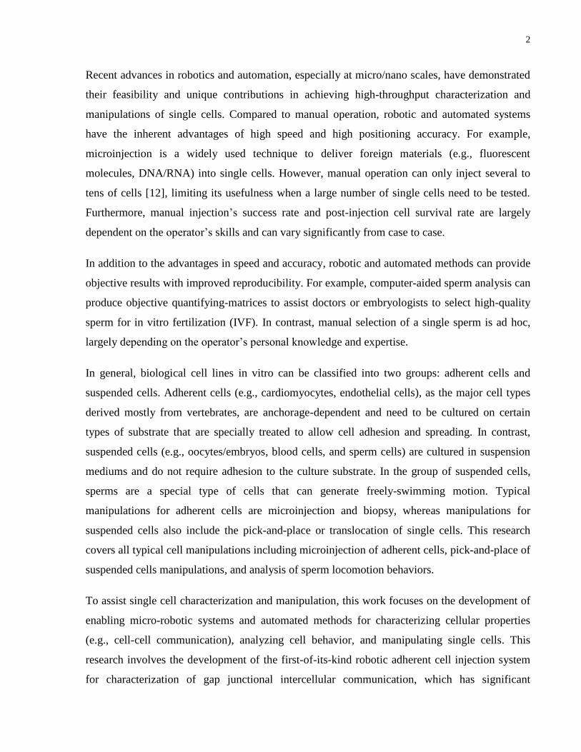
Recent advances in robotics and automation, especially at micro/nano scales, have demonstrated
their feasibility and unique contributions in achieving high-throughput characterization and
manipulations of single cells. Compared to manual operation, robotic and automated systems
have the inherent advantages of high speed and high positioning accuracy. For example,
microinjection is a widely used technique to deliver foreign materials (e.g., fluorescent
molecules, DNA/RNA) into single cells. However, manual operation can only inject several to
tens of cells [12], limiting its usefulness when a large number of single cells need to be tested.
Furthermore, manual injection‟s success rate and post-injection cell survival rate are largely
dependent on the operator‟s skills and can vary significantly from case to case.
In addition to the advantages in speed and accuracy, robotic and automated methods can provide
objective results with improved reproducibility. For example, computer-aided sperm analysis can
produce objective quantifying-matrices to assist doctors or embryologists to select high-quality
sperm for in vitro fertilization (IVF). In contrast, manual selection of a single sperm is ad hoc,
largely depending on the operator‟s personal knowledge and expertise.
In general, biological cell lines in vitro can be classified into two groups: adherent cells and
suspended cells. Adherent cells (e.g., cardiomyocytes, endothelial cells), as the major cell types
derived mostly from vertebrates, are anchorage-dependent and need to be cultured on certain
types of substrate that are specially treated to allow cell adhesion and spreading. In contrast,
suspended cells (e.g., oocytes/embryos, blood cells, and sperm cells) are cultured in suspension
mediums and do not require adhesion to the culture substrate. In the group of suspended cells,
sperms are a special type of cells that can generate freely-swimming motion. Typical
manipulations for adherent cells are microinjection and biopsy, whereas manipulations for
suspended cells also include the pick-and-place or translocation of single cells. This research
covers all typical cell manipulations including microinjection of adherent cells, pick-and-place of
suspended cells manipulations, and analysis of sperm locomotion behaviors.
To assist single cell characterization and manipulation, this work focuses on the development of
enabling micro-robotic systems and automated methods for characterizing cellular properties
(e.g., cell-cell communication), analyzing cell behavior, and manipulating single cells. This
research involves the development of the first-of-its-kind robotic adherent cell injection system
for characterization of gap junctional intercellular communication, which has significant
3
implications for screening drug efficacy for cardiac diseases caused by the dysfunction of cell-
cell communication. Additionally, this thesis also introduces a robotic system to pick-and-place
mammalian oocytes or embryos for cryopreservation. Besides, this research also includes the
development of computer vision algorithms for tracking both sperm head and tail to facilitate the
analysis of sperm locomotion behaviors for IVF applications.
4
1.2 Characterization of Gap Junctional Intercellular Communication
Gap junctional intercellular communication (GJIC) exists in most mammalian tissues. Gap
junction is a specialized intercellular channel formed by the juxtaposition of two half channels
called connexons [13], [14]. Gap junctions are critical to several physiological roles, including
impulse propagation in cardiac and neuronal tissue [15], regulation of embryonic development
[16], homeostasis [17], and regulation of cellular proliferation [18]. Disorders of GJIC have been
associated with many pathological conditions and vital diseases, such as cardiac arrhythmias
[19], [20], which are a leading cause of cardiac morbidity and sudden death [21].
Gap junctions provide a direct pathway for electrical and metabolic signaling between
connecting adjacent cells. Similar to ion channels, gap junctions are also ionic conduits [22].
However, unlike conventional ion channels, the selectivity of gap junctions for small ions (either
positively or negatively charged) is minor compared to the selectivity of Na+ and K
+ channels.
The size of gap junction channels is much larger than that of conventional ion channels (100-150
Å vs. 3-5 Å) [23].
Gap junctions facilitate both diffusion of small molecules and conduction of ions between
adjacent cells. Intercellular diffusion is attributed to essentially only through gap junctions,
whereas sodium channels also contribute to conduction in the heart. In addition to ionic
communication, gap junctions are molecular sieves that allow small hydrophilic chemical
molecules, such as metabolites and second messengers (e.g., triphosphate inositol), to pass [24].
Gap junctions are regulated by gating that is referenced as open, semi-open, and closed
configurations. When all the channels in a gap junction gate are closed, diffusion of permeants
from cell to cell is halted. Experimentally, gating is commonly induced by imposing a voltage
gradient across the junction. In addition to gating, the gap junction-mediated intercellular
communication is also regulated by intracellular calcium, pH, and phosphorylation [25].
GJIC is regulated by the number of gap junction channels in the membrane, the functional state
of gap junctions, and their permeability [26]. The measurement of GJIC has been studied for
decades by using a number of methods, such as dye transfer through microinjection [27], the
scrape/scratch method [28], electroporation [29], fluorescence redistribution after photobleaching
[30], and conductance measurement by dual-cell patch clamp [31]. Among these techniques,
5
microinjection of membrane-impermeable, non-toxic tracers into single cells has been the most
commonly used technique for identifying and mapping GJIC for a wide variety of cells [32]. The
microinjection method is considered superior to other techniques because of the following
reasons: 1) microinjection permits the correlation of morphological and functional data from
individual cells; 2) the technique enables kinetic studies aimed at evaluating the transfer rate
from one cell to another; and 3) in microinjection, the level of cell communication is expressed
as number of dye-coupled cells, permitting the direct comparison of GJIC in different cell types
[33].
However, microinjection has stringent skill requirements, low cell viability rate, and poor
reproducibility [12]. Manual microinjection is typically used for injecting a few or tens of cells
per experiment, limiting its usefulness when a large number of cells need to be tested for GJIC
assessment. In this research, I have developed a robotic microinjection system and technique, for
the first time, to enable the injection of hundreds of adherent cells per experiment rapidly and
accurately. The automated system is operated via computer mouse clicking for indicating target
cells for microinjection. Training a user who has no skills in microinjection takes ~15 min, and
after a few hours of operation, the user can readily become proficient at operating the system to
perform microinjection with high success rates.
6
1.3 Robotics and Automation for in vitro Fertilization
The World Health Organization reports that averagely 8~10% of couples worldwide experience
infertility [34]. And data from the US National Centre for Disease Control shows that one out of
eight North American couples seek medical treatment for infertility. Since the birth of Louise
Brown, conceived using in vitro fertilization (IVF) pioneered by Noble Prize Laureate – Robert
Edwards, the outcomes and impact of assisted reproductive theologies (ART) have been
remarkable [35][36]. Despite the significant progress in ART, most operations in IVF clinics are
still performed manually. Treatment outcomes largely rely on expert knowledge and experienced
hands. To address the bottleneck problem in IVF, this research involves the development of
robotic systems and automated methods aiming to standardize two IVF routine procedures: (1)
vitrification of oocytes or embryos, and (2) analysis of sperm locomotive behaviors.
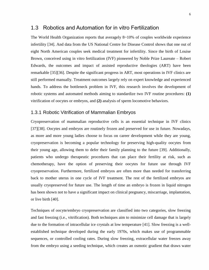
1.3.1 Robotic Vitrification of Mammalian Embryos
Cryopreservation of mammalian reproductive cells is an essential technique in IVF clinics
[37][38]. Oocytes and embryos are routinely frozen and preserved for use in future. Nowadays,
as more and more young ladies choose to focus on career development while they are young,
cryopreservation is becoming a popular technology for preserving high-quality oocytes from
their young age, allowing them to defer their family planning to the future [39]. Additionally,
patients who undergo therapeutic procedures that can place their fertility at risk, such as
chemotherapy, have the option of preserving their oocytes for future use through IVF
cryopreservation. Furthermore, fertilized embryos are often more than needed for transferring
back to mother uterus in one cycle of IVF treatment. The rest of the fertilized embryos are
usually cryopreserved for future use. The length of time an embryo is frozen in liquid nitrogen
has been shown not to have a significant impact on clinical pregnancy, miscarriage, implantation,
or live birth [40].
Techniques of oocyte/embryo cryopreservation are classified into two categories, slow freezing
and fast freezing (i.e., vitrification). Both techniques aim to minimize cell damage that is largely
due to the formation of intracellular ice crystals at low temperature [41]. Slow freezing is a well-
established technique developed during the early 1970s, which makes use of programmable
sequences, or controlled cooling rates. During slow freezing, extracellular water freezes away
from the embryo using a seeding technique, which creates an osmotic gradient that draws water
7
out of the cell until it finally freezes without the formation of intracellular ice crystals [42]. This
procedure requires sophisticated equipment to control the freezing rate, which ranges between
0.3 and 1.0 µ°C/min, and produces a relatively poor survivability rate [43].
On the other hand, vitrification or fast freezing is a more effective cryopreservation method, first
reported in 1985 [44]. Vitrification is considered superior to slow freezing because it vitrifies the
oocyte/embryo with no crystal formation during freezing. The addition of cryoprotectants in
vitrification increases the cytosol viscosity and makes the vitrified oocyte/embryo syrupy. When
directly freezing oocytes/embryos in liquid nitrogen, the syrupy content inside the cell forms
amorphous ice instead of ice crystals, which minimize the vital damage to the cell during
freezing.
At present, oocyte/embryo vitrification is done manually in IVF clinics. An operator looks
through the microscope eyepieces and manipulates oocytes/embryos using a Stipper®
micropipette or mouth pipette. Manual operation for oocyte/embryo vitrification is a demanding
and tedious task, for the following reasons:
(1) vitrification requires precise washing sequences and strict timings in each vitrification
solution (VS) because the cryoprotectants (e.g., DMSO) are toxic and can significantly
damage the cell viability if overexposed in vitrification solution;
(2) because of their small size (about 150 µm), oocytes/embryos can be difficult to observe
and manipulate, especially when the oocytes/embryos locations are dynamically changing
during micropipette aspiration and dispensing;
(3) washing oocytes/embryos with the highly viscous VS can cause osmotic shock to the
cells, which can damage the cell survivability in vitrification;
(4) the manual process has stringent skill requirements, and success rate and cell survival rate
vary across different operators. In IVF clinics, processing an embryo/oocyte in
cryoprotectant medium typically takes a highly skilled embryologist 10 to 15 minutes.
To address the shortcomings of manual vitrification, this research focuses on the development of
a robotic system for automatically pick-and-placing the oocytes/embryos through various
vitrification solutions.

8
1.3.2 Quantitative Analysis of Sperm Locomotion Behavior
In natural fertilization, a healthy sperm overcomes the physiological and biological selection
barriers, actively seeks out and fertilizes an egg. Sperm selection occurs naturally in this
procedure. However, for couples having infertility issues, assisted reproduction technologies are
required to address their reproductive needs. For example, in intracytoplasmic sperm injection
(ICSI), an embryologist selects a single sperm cell and injects it directly into an oocyte (i.e., egg
cell) to overcome issues such as male infertility [45]. These assisted reproduction technologies
bypass the natural sperm selection barriers and demand expertise knowledge from the operator to
select high-quality sperms. The criteria for sperm quality assessment provided by the World
Health Organization are vitality, morphology, and motility [46]. A widely used method for sperm
selection is motile sperm organelle morphology examination (MSOME) [47][48][49][50]. Sperm
motility is also a commonly used criterion for sperm quality assessment. A motility grade is
often used as a specified measure and classified into four grades:
Grade 1: sperm with fast progressive movements;
Grade 2: sperm with slow progressive movements;
Grade 3: sperm with slow non-progressive movements (i.e., with curved motion);
Grade 4: sperms are immobile and fail to move at all.
Besides sperm assessment based on morphology and motility, another method for selecting a
healthy sperm is based on the analysis of sperm DNA integrity. Some of the DNA analysis
methods assess sperm DNA quality directly, such as the TUNEL assay and the sperm chromatin
structure assay. Some other methods indirectly measure sperm DNA quality. For instance,
Huszar‟s group recently proposed a hyaluronic acid (HA) assay [51]. Among a consecutive
series of studies on HA-based sperm assay, researchers in Huszar‟s group indicated that HA
assay permits the selection of healthy sperm with no DNA damage [52][53]. In their research,
sperms that bind to HA microdots are proven to have a higher level of DNA integrity compared
to those unbound sperms. In clinical HA-based sperm selection, a number of healthy sperms‟
heads bind to the HA microdot and lose their progressive movement despite vigorous tail
beating. In this case, the sperm tail beating movement becomes the only indicator to differentiate
the HA-bound sperms from each other.
9
The past few decades have witnessed the development of computer-assisted sperm analysis
(CASA) methods for measuring both sperm morphology and motility [54]. CASA utilizes
automated systems to digitize successive images of sperm, process and analyze the information,
and provide the accurate and objective value for individual sperm cell. Since the 1970s, many
algorithms have been developed to track sperm trajectories, measure sperm velocities, and
analyze sperm morphology. Shi et al. reported a robust single-sperm tracking algorithm based on
a four-class thresholding method to extract a single sperm in a region of interest [55]. The
nearest neighbor method is complemented with a speed-check feature to aid tracking in the
presence of additional sperm or other particles. In another study, Nafisi et al. demonstrated a
template matching algorithm for sperm tracking. The algorithm is insensitive to image
acquisition conditions [56]. Existing algorithms for sperm tracking are largely limited to sperm
head tracking. The small size (≤ 1 µm in thickness) and low contrast of sperm tails under optical
microscopy makes tracking sperm tails challenging.
This research also involves the development of a new automated analysis method by tracking
both sperms‟ heads and tails. With this automated method, users can obtain objective
information about sperm locomotion behaviors. This research has significant applications to
assist the selection of high-quality sperm by unifying the sperm motility analysis with DNA
assessment techniques (e.g., HA assay) in IVF clinics.
10
1.4 Previous Methods for Robotic Cell Manipulation
The past decade has seen significant development of robotic cell manipulation systems and
automated characterization techniques for patterning, grasping, measuring, and injecting
individual cells [57][58][59][60]. In general, the strategies for single cell manipulations and
characterization can be classified into five categories: mechanical, fluidic, electrical, optical and
magnetic.
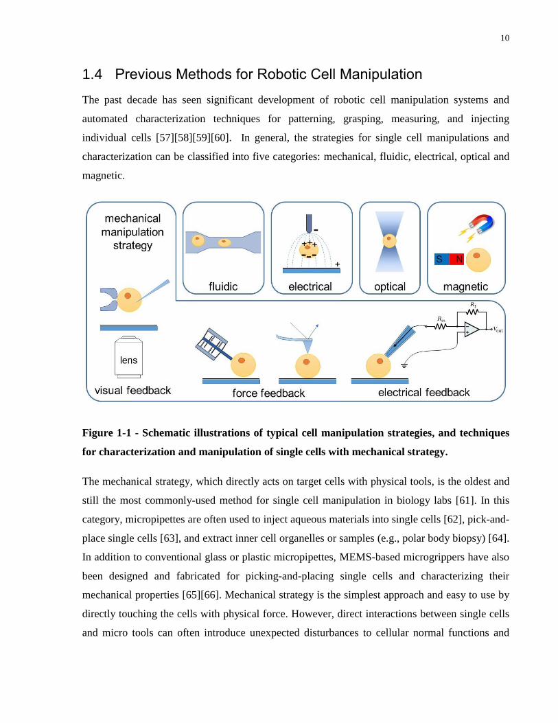
Figure 1-1 - Schematic illustrations of typical cell manipulation strategies, and techniques
for characterization and manipulation of single cells with mechanical strategy.
The mechanical strategy, which directly acts on target cells with physical tools, is the oldest and
still the most commonly-used method for single cell manipulation in biology labs [61]. In this
category, micropipettes are often used to inject aqueous materials into single cells [62], pick-and-
place single cells [63], and extract inner cell organelles or samples (e.g., polar body biopsy) [64].
In addition to conventional glass or plastic micropipettes, MEMS-based microgrippers have also
been designed and fabricated for picking-and-placing single cells and characterizing their
mechanical properties [65][66]. Mechanical strategy is the simplest approach and easy to use by
directly touching the cells with physical force. However, direct interactions between single cells
and micro tools can often introduce unexpected disturbances to cellular normal functions and
11
damage cell viabilities, especially when the experiments are conducted by users with little
micromanipulation experience.
The second group of manipulation strategies use microfluidic devices to move single cells within
constrained channels [67][68]. In microfluidic manipulations, researchers have applied flow-
induced forces to characterize the cellular mechanical properties [69][70]. For automation in
IVF, such as for vitrification of embryos and sperm quality assessment, microfluidic approaches
have also become increasingly popular. The advantages of using microfluidic devices include the
pre-patterned motion paths, minimal volume requirement, reduction of material costs, and
decreased reaction time with high surface-to-volume ratio [71]. However, the difficulties in
introduction and extraction of single cells on microfluidic devices greatly limit the practicality
for targeting single cells of interest [72]. Moreover, the measured and processed single cells are
difficult to be extracted from the large cell populations.
Different from mechanical and fluidic manipulations, which involve physical contact with single
cells, electrical, optical and magnetic manipulations are capable of interacting with single cells in
an untethered way. Electrical manipulations, such as dielectrophoresis (DEP) [73], generate a
non-uniform electrical field to exert electrical forces on dielectric particles or cells. DEP
manipulates cells without contacting them and is easy to control well [74]. However, the
generated forces strongly depend on surrounding medium, cell electrical properties, cell size and
shapes [75].
Optical manipulations, or optical tweezers, use a highly focused laser beam to produce an
attractive or repulsive force depending on a refractive index mismatch to physically hold and
move micro/nano-objects [76]. Although the optical tweezers can accurately position single cells
with minimal invasiveness, this technique is limited in force generation (pN levels), and
increasing laser power for larger force generation has the risk of laser-induced cell damage.
Magnetic nanoparticles, after introduced into cells, can be moved by magnetic forces generated
by controlled magnetic fields. Because cells do not contain magnetic structures, the force is
specifically applied to the internalized magnetic particles. Magnetic tweezers have been used for
manipulating intracellular structures such as chromatin [77] and phagosomes [78]. Although
most magnetic tweezers reported in literature apply forces in one direction only, there are a
growing number of systems that allow 2D and 3D manipulation [79], [80]. One major limitation
12
of magnetic manipulation lies in the positioning accuracy and force resolutions. To solve this
problem, pioneering researchers in Nelson‟s group at ETH Zurich, Sitti‟s group at Carnegie
Mellon, and Kumar‟s group at UPenn have worked to improve the control system for moving
single [82] or multiple [83][84] untethered microrobots to assemble microobjects [85] or deliver
drugs to single cells and tissues [86]. The magnetic microrobots had also been built with
bioinspired flagellar shapes to increase their mobility in a liquid environment at micro/nano scale
[87][88]. Japanese researchers at Nagoya University also combined the magnetic approach with
microfluidic chips to build an on-chip microrobot system [89] for targeting single cell
mechanical characterization [90].
Compared with manual operation and other cell manipulation strategies (e.g., microfluidics,
magnetic tweezers, laser trapping and dielectrophoresis), robotic cell manipulation systems using
mechanical strategies have been demonstrated to overcome their limitations (e.g., cell damage,
cell loss, poor specificity) and be capable of conducting more complex tasks [57]. Direct
manipulation using mechanical strategies, such as microassembly of microobjects,
microinjection of cells, and pick-and-place of single cells, provides a more intuitive and
straightforward solution.
Robotic micromanipulations using mechanical strategy can be further classified into three
categories depending on their distinct feedback modes. The classifications of robotic
manipulation using mechanical strategy are summarized in Table 1. Early studies in robotic
micromanipulation used visual feedback for automation. Because all micromanipulation tasks
are conducted under microscopes (either optical or electron microscope), visual feedback is the
most useful approach for building closed-loop schemes because imaging feedback can provide
plentiful information for tracking cell locations and positioning manipulation end-effectors.
However, microscopy imaging often has a limited depth of field and a small field of view, posing
critical challenges in searching and locating end-effectors both in the image plane and in depth.
Therefore, early research with visual feedback are mainly focused on microassembly of
relatively large objects or microinjection of large cells such as mouse oocytes and zebrafish
embryos.
13
Table 1 - Previous Methods for Robotic Micromanipulations using Mechanical Strategy
Technical
Classification Methods Description Applications References
Force
Feedback
MEMS-
Based
Devices
silicon-based MEMS devices measure
forces at a high resolution of nano-
Newton level; PDMS-based probes or
micro-posts devices can also measure
forces by visually tracking shape
changes; fabrication processes are
complex; devices are easy to damage.
microassembly;
microinjection;
cellular
mechanical
characterization
[91] [92]
[93] [94]
[95] [96]
[97] [98]
[99] [100]
Piezoelectric
Materials
(e.g., PVDF)
force sensing modules usually
integrated on the micropipette holders
or cell holding devices; relatively
easier to fabricate; measurement
resolution ranges from a few to
several hundreds of micro-Newton.
microinjection;
cellular
mechanical
characterization
[101] [102]
[103] [104]
[105] [106]
[107]
AFM
highest force measurement resolution;
limited applications; High equipment
cost; AFM probes can be modified
into various shapes; applications also
performed under electron microscope
cellular or
intracellular
mechanical
characterization;
microinjection
[108] [109]
[110] [111]
[112] [113]
[114] [115]
[116] [117]
Electrical
Feedback
Impedance
Measurement
Electrode inserting into micropipette
to measure the impedance change;
Monitoring impedance change can
detect cell-pipette contact, pipette tip
breakage, and pipette clogging
microinjection;
selectively
isolate cells
from cell
cultures
[118] [119]
[120] [121]
[119]
I-V Curve
Monitoring +
Visual
Feedback
electrode inserting into glass
micropipette was used for monitoring
cell-micropipette contact and
realizing electroporation
microinjection
of sea urchin
eggs with
fluorescent dye
[122]
Planar Patch-
Clamp
System +
AFM
planar patch-clamp system can both
record electrical signals and exchange
intracellular solution; AFM generates
force stimuli with controllable
patterns and magnitudes; AFM
scanning of the single cell provides
detailed morphological information.
electrical
recordings of
whole-cell
current of
potassium ion
channel
[123]
Visual
Feedback
Computer
Vision +
Visual
Servoing
No extra device/equipment cost;
Optical microscopy has limited depth
of field and small field of view;
Z-position information can only be
estimated; Applications limited to
relative large objects or cells (e.g.,
embryos); Image-based visual
feedback requires system calibration.
microassembly;
microinjection;
pick-and-place
of single cells;
[124] [125]
[126] [127]
[128] [129]
[130] [131]
[132] [133]
[134] [135]
14
As MEMS technology advanced during the first decade of the twenty-first century, force
feedback was introduced into robotic micromanipulation by integrating MEMS-based force
sensors into end effectors. The accurate and high-resolution force measurement provided an
improved solution in the determination of relative Z positions between end-effectors and cells.
Additionally, micromanipulation with MEMS-based force sensors also has the inherent
advantages in characterizing the mechanical properties of single cells because the force-
deformation curve can be easily achieved in experiments. Despite their significant advantages,
MEMS-based force sensors did not reach the large-scale adoption in biological labs or clinics
because of the customized force sensors‟ time consuming and complex fabrication processes. As
an alternative solution to MEMS-based force sensors, researchers also tried using piezoelectric
materials (e.g., PVDF) to make cantilever structures on end-effector holders or thin films on cell
culture devices for measuring forces. PVDF sensors are relatively easier to fabricate, but they
have reduced force measurement resolution, often at several tens of micro-Newtons. The third
type of force feedback uses AFM (Atomic Force Microscopy) systems, which have very high
force measurement resolutions. By modifying the AFM probes into special shapes (e.g.,
nanoneedle, nanofork, and nanoknife), Japanese researchers in Fukuda‟s lab have conducted very
interesting studies, such as the quantification of adhesion forces of single cells, single cell
surgery with modified AFM nanofork or nanoknife. However, AFM is expensive and cannot
achieve many other demanding manipulation tasks including microinjection and pick-and-place
of cells, which limits its practicality in typical biological labs or regular clinics.
In addition to visual and force feedback, other researchers also used electrical feedback to assist
in the detection of cell-micropipette contact. In this method, positive electrodes are often inserted
into micropipettes and connected to electrical amplifying circuits and measurement equipment.
The negative or ground electrodes are placed in the cell culture devices. The system monitors the
changes in micropipette tip resistance/impedance to detect cell-micropipette contact, tip breakage
or tip clogging. In addition to monitoring the changes of electrical signals, this method can also
provide extra functions such as electroporation and patch clamping. However, robotic
manipulations using electrical feedback usually require high-specification measurement
equipment because the weak bioelectrical signals easily obscured by ambient electromagnetic
noise. Moreover, the introduction of an electric field can also disturb normal cellular functions
such as gap junctional intercellular communications.

15
Compared to force and electrical feedback, visual feedback works as the most basic approach to
achieve robotic and automated cell manipulations. Robotic manipulation of cells with visual
feedback does not require additional sensing or measurement equipment, making it the most
suitable approach for large-scale adoption in biology labs and clinics from a cost standpoint.
16
1.5 Opportunities for Innovations in Robotic Cell Manipulation
Although many algorithms and techniques have been developed for robotic cell manipulations,
several key issues still exist which limits the practical adoption of robotic cell characterization
and manipulation technologies in biology labs and clinics. These technical issues are:
In order to realize practical adoption in biology labs and clinics, complicated force
sensors or electrical feedback should be avoided and research needs to be focused on
visual feedback approaches.
To achieve robotic manipulation with visual feedback, novel methods are required to
search and detect low-contrast objects (e.g., end-effector tips with various shapes and
fast-swimming motile sperms) in a small field of view under optical microscopy with a
limited depth of field.
To realize visual-servoing robotic manipulation, the relative vertical positions of end-
effectors and cells (Z-position) must be accurately determined and the positioning errors
in the X-Y plane must be well compensated.
Novel robotic manipulation systems must have high throughput capability in order to
achieve statistically significant results for investigating the heterogeneous cell behaviors.
The cell‟s response to external environment (e.g., embryo volume changes due to osmotic
pressure) and behavior changes (e.g., sperm tail beating increases after binding to HA)
must be closely monitored during cell manipulations in order to achieve the optimal
performance for each target cells.
The prerequisite step for all micromanipulations, which is how to locate end-effector tips,
was performed manually. End-effectors, such as micropipettes and microgrippers, must
be first searched and located under microscopy imaging before any micromanipulation
task is performed. There is no robotic algorithm for automatically locating end-effector
tips.
17
1.6 Research Objectives
In this research, I aimed to solve the aforementioned technical issues and use the new solutions
to build robotic systems and automated methods for characterization and manipulation of single
adherent and suspended cells. Specific objectives of this research include:
To develop automated method for automatically locating end-effector tips.
To develop computer vision based contact detection algorithms for determination of
relative Z-positions of end-effector tips and single cells.
To build an automated system for robotic injection of adherent cells to measure gap
junctional intercellular communications.
To achieve a high throughput in microinjection of adherent cells with a high success rate,
a high reproducibility, and a high post-injection survival rate.
To use the robotic microinjection system for screening the efficacy of selected drug
molecules based on the measurement of gap junctional communications.
To develop algorithms for controlled aspiration and positioning suspended cells inside a
micropipette.
To build an automated system for robotic processing of mouse embryos for vitrification.
To develop 3D tracking algorithms for analyzing the morphological changes of oocytes
or embryos during vitrification.
To develop computer vision tracking algorithms for automated analysis of sperm head
and tail locomotion behavior.

18
1.7 Dissertation Outline
An overview of the ensuing chapters is as follows:
Chapter 2 explains the new solution for automatically locating end-effector tips. Micropipettes
and microgrippers were used as example end-effectors to evaluate the performance of proposed
auto-locating method. Guidelines for implementation of this method are provided at the end of
the chapter.
Chapter 3 presents a robotic injection system for characterization of GJIC. Two new vision-
based contact detection algorithms are discussed in this chapter. The performance of the system
is evaluated by injecting three distinct adherent cell lines. Preliminary testing results on
screening the selected drugs are reported in this chapter.
Chapter 4 describes a robotic approach for automatically pick-and-place embryos for
vitrification. The implementation of auto-locating end-effector tips method and vision based
contact detection is discussed in this chapter. New methods for tracking embryos in vitrification
solutions are explained. Test results on system operation speed, post-thawing survival rate, and
development rate are also presented.
Chapter 5 reports automated analysis method for quantifying sperm locomotion behaviors.
Experimental results on free-swimming sperm and HA-bond sperm are compared in this chapter,
confirming the significant potentials to unify the sperm motility analysis with DNA integrity
assessment.
Chapter 6 concludes the entire thesis work with a summary of contributions. Future research
directions are also discussed in this chapter.
19
Chapter 2 Automatically Locating End-effector Tips in Micromanipulation
This chapter discusses an automated solution for automatically locating end-effector tips in
micromanipulation. The performance of the automated function was tested by using various end-
effectors under three major types of microscopy imaging modes. The newly developed auto-
locating functions are proven to be effective for avoiding tip breakage, saving operation time,
and eliminating human involvement. Special guidelines for implementation of this auto-locating
function are provided at the end of this chapter.
The following section is based on the text from the following publication:
J. Liu, Z. Gong, K. Tang, Z. Lu, C. Ru, J. Luo, S. Xie, and Y. Sun, "Locating end-effector tips in
robotic micromanipulation," IEEE Transactions on Robotics, Vol. 30, pp. 125-30, 2014.
20
Automatically Locating End-Effector Tips in 2
Micromanipulation
In robotic micromanipulation, end-effector tips must be first located under microscopy imaging
before manipulation is performed. The tip of micromanipulation tools is typically a few
micrometers in size and highly delicate. In all existing micromanipulation systems, the process
of locating the end-effector tip is conducted by a skilled operator, and the automation of this task
has not been attempted. This chapter presents a technique to automatically locate end-effector
tips. The technique consists of programmed sweeping patterns, motion history image end-
effector detection, active contour to estimate end-effector positions, autofocusing and quad-tree
search to locate an end-effector tip, and, finally, visual servoing to position the tip to the center
of the field of view. Two types of micromanipulation tools (micropipette that represents single-
ended tools and microgripper that represents multi-ended tools) were used in experiments for
testing. Quantitative results are reported in the speed and success rate of the auto-locating
technique, based on over 500 trials. Furthermore, the effect of factors such as imaging mode and
image processing parameter selections was also quantitatively discussed. Guidelines are
provided for the implementation of the technique in order to achieve high efficiency and success
rates.
21
2.1 Introduction
Micromanipulation tools such as micropipettes and microelectromechanical systems (MEMS)
microgrippers are commonly used in the manipulation of micro-scaled objects. Locating the tip
of these end-effectors under microscopy must be conducted before micromanipulation initiates.
In previous manual and robotic micromanipulation, locating the tip of end-effectors (searching,
positioning, and focusing) is a manual procedure performed by skilled operators. Because of the
small size and fragility of micromanipulation end-effectors, manually locating end-effector tips
has high skill requirements, is time-consuming, and can cause end-effector breakage. Despite the
progress made in robotic micromanipulation [111][136][95][137][138], the automation of the
procedure of locating end-effector tips has not been investigated. Most end-effectors used in
micromanipulation have micrometer-sized tips (single or multi-ended). For instance,
micropipette tips used in cell manipulation and microgrippers for assembly tasks are usually a
few micrometers in diameter (see Fig. 2-1). The tiny tip of these end- effectors is difficult to
locate, particularly under high magnifications in microscopy imaging. When the end-effector
collides into other objects (e.g., wafer substrate, glass slide, petri dish, or other end-effectors)
during the process of locating the end-effector and micromanipulation, the tip can be easily
damaged and requires replacement. Hence, automation techniques to readily locate the end-
effector tips are necessary to reduce human intervention and achieve autonomous robotic
micromanipulation.
Figure 2-1 - Example end-effectors used in micromanipulation. Their micrometer-sized tips
must be located first before micromanipulation initiates. (a) Microgrippers for pick-and-place of
small objects. The grasped particles are 10 µm in diameter. (b) Micropipettes for manipulating
biomaterials.
22
Automatically locating end-effectors requires visual detection and focus estimation to determine
the end-effector‟s position in three dimensions. Several techniques have been reported to visually
detect and track micro objects. Ni et al. proposed an iterative closest point algorithm to track a
microgripper‟s position [139]. The algorithm requires the use of an additional dynamic vision
sensor (silicon retina). This special hardware requirement makes the algorithm unsuitable for
micromanipulation tasks that rely on standard vision systems. Microgrippers with complex
features were also tracked using the template matching method for micro-assembly tasks
[140][141]. Our experimental results indicate that the template matching is ineffective to track
objects without distinct features (e.g., micropipettes). In another related work [142], a
generalized Hough transform was applied to detect end-effector tips. However, the approach can
only detect objects with regular shapes (i.e., lines or circular shapes). Algorithms based on one-
class support vector machines [143], shearlet multiscale directional transform [144], and the
Kalman filter [145] have also been used to detect or track objects under microscopy imaging.
However, these algorithms are only suitable to process in-focus images. In the task of locating
end-effector tips, the end-effector often is partially or entirely out of focus. In addition, the
shapes and end-effectors‟ direction of entering the field of view (FOV) also vary with different
micromanipulation tasks. These unique requirements call for the development of techniques to
automatically locate end-effectors under microscopy.
This chapter presents a technique that is capable of searching for out-of-FOV, out-of-focus, and
low-contrast end-effectors. A detection algorithm based on a motion history image (MHI) and an
active con- tour model is used to search for the end-effector. Through estimating the end-effector
tip‟s location and the use of an adaptive quadtree autofocusing algorithm, the tip of the end-
effector is detected and moved to the center of the FOV and brought in focus. This chapter
describes in more detail algorithm comparisons and experimental results. Micropipettes and
MEMS microgrippers are used as example end-effectors to evaluate the performance of the
technique. Experimental results from the over 500 trials under three common imaging modes
(bright field, differential interference contrast or DIC, and phase contrast) demonstrate that the
technique is capable of automatically locating end-effectors under microscopy imaging with high
efficiency and accuracy.
23
2.2 System Design
2.2.1 System Architecture
Figure 2-2 - (a) Schematic illustration of the experimental setup. (b) System picture.
As shown in Fig. 2-2, the micromanipulation system setup consists of a standard inverted
microscope (TE2000-S, Nikon) with motorized focus control and a CMOS camera connected
24
(scA1300-32gm, Basler; resolution: 1200×900). Objectives of 4×, 10×, and 20×are used and
have depths of field of 55.5, 13.5, 5.5µm, respectively. An end-effector (i.e., a micropipette or a
microgripper in this study) is mounted on a motorized 3-DOF micromanipulator (Sutter MP285)
at a tilting angle of 30◦. Movements performed in the automation procedure consist of X, Y, and
Z translation motions of the end-effector as well as adjustment of the microscope‟s focus.
2.2.2 Overall Sequence
The end-effector is initially at or above the focal plane. The search range is established within a
4-mm cubic workspace (−2 mm ≤ x ≤ +2 mm, −2 mm ≤ y ≤ +2 mm, 0 mm ≤ z ≤ +4 mm) [see
Fig. 2-2(a)]. When setting up an end-effector in micromanipulation, it is feasible for the operator
to readily position the end-effector tip to within this 4-mm cube workspace with unaided eyes
and reasonable care. The automated procedure has two main steps: end-effector detection and
autofocus adjustment. Fig. 2-3 summarizes the overall sequence.
Figure 2-3 - Overall sequence for auto-locating end-effector tips contains two major steps.
(1) End-Effector Detection: In the detection step, the end-effector is swept in the X–Y plane. An
algorithm based on an MHI is used to detect the presence of end-effector in the FOV. In some
cases, the end-effector cannot be detected when it is far away from the focal plane. When this
occurs, the focal plane is moved upwards, and horizontal X–Y sweep is repeated. The step size
of focus adjustment depends on the depth of field of the microscope objectives. In our system,
the step size for 4×, 10× and 20× objectives is set as 50, 10, and 5 µm, respectively. When a
moving object is detected in multiple continuous frames of images during the sweeping of the
end-effector, the end-effector is considered to be present in the FOV.
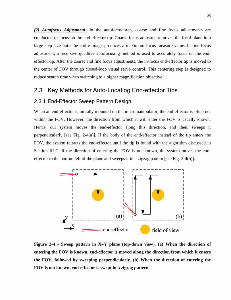
25
(2) Autofocus Adjustment: In the autofocus step, coarse and fine focus adjustments are
conducted to focus on the end-effector tip. Coarse focus adjustment moves the focal plane in a
large step size until the entire image produces a maximum focus measure value. In fine focus
adjustment, a recursive quadtree autofocusing method is used to accurately focus on the end-
effector tip. After the coarse and fine focus adjustments, the in-focus end-effector tip is moved to
the center of FOV through closed-loop visual servo control. This centering step is designed to
reduce search time when switching to a higher magnification objective.
2.3 Key Methods for Auto-Locating End-effector Tips
2.3.1 End-Effector Sweep Pattern Design
When an end-effector is initially mounted on the micromanipulator, the end-effector is often not
within the FOV. However, the direction from which it will enter the FOV is usually known.
Hence, our system moves the end-effector along this direction, and then, sweeps it
perpendicularly [see Fig. 2-4(a)]. If the body of the end-effector instead of the tip enters the
FOV, the system retracts the end-effector until the tip is found with the algorithm discussed in
Section III-C. If the direction of entering the FOV is not known, the system moves the end-
effector to the bottom left of the plane and sweeps it in a zigzag pattern [see Fig. 2-4(b)].
Figure 2-4 - Sweep pattern in X–Y plane (top-down view). (a) When the direction of
entering the FOV is known, end-effector is moved along the direction from which it enters
the FOV, followed by sweeping perpendicularly. (b) When the direction of entering the
FOV is not known, end-effector is swept in a zigzag pattern.
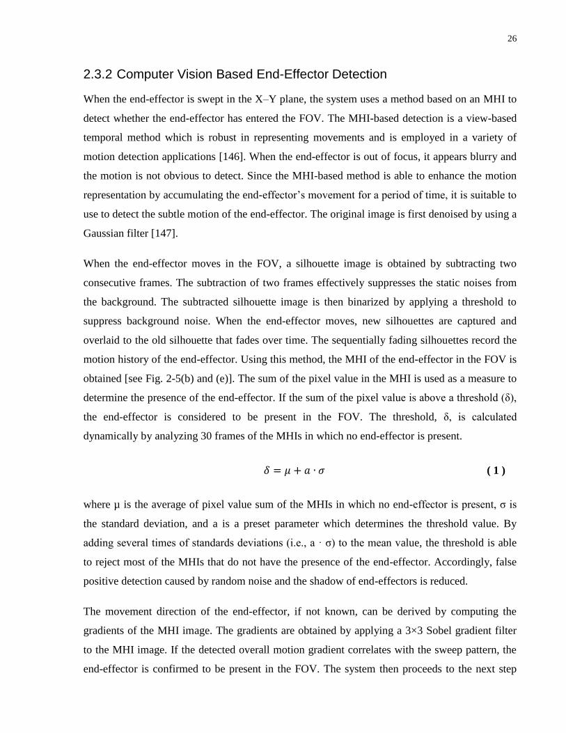
26
2.3.2 Computer Vision Based End-Effector Detection
When the end-effector is swept in the X–Y plane, the system uses a method based on an MHI to
detect whether the end-effector has entered the FOV. The MHI-based detection is a view-based
temporal method which is robust in representing movements and is employed in a variety of
motion detection applications [146]. When the end-effector is out of focus, it appears blurry and
the motion is not obvious to detect. Since the MHI-based method is able to enhance the motion
representation by accumulating the end-effector‟s movement for a period of time, it is suitable to
use to detect the subtle motion of the end-effector. The original image is first denoised by using a
Gaussian filter [147].
When the end-effector moves in the FOV, a silhouette image is obtained by subtracting two
consecutive frames. The subtraction of two frames effectively suppresses the static noises from
the background. The subtracted silhouette image is then binarized by applying a threshold to
suppress background noise. When the end-effector moves, new silhouettes are captured and
overlaid to the old silhouette that fades over time. The sequentially fading silhouettes record the
motion history of the end-effector. Using this method, the MHI of the end-effector in the FOV is
obtained [see Fig. 2-5(b) and (e)]. The sum of the pixel value in the MHI is used as a measure to
determine the presence of the end-effector. If the sum of the pixel value is above a threshold (δ),
the end-effector is considered to be present in the FOV. The threshold, δ, is calculated
dynamically by analyzing 30 frames of the MHIs in which no end-effector is present.
( 1 )
where µ is the average of pixel value sum of the MHIs in which no end-effector is present, σ is
the standard deviation, and a is a preset parameter which determines the threshold value. By
adding several times of standards deviations (i.e., a · σ) to the mean value, the threshold is able
to reject most of the MHIs that do not have the presence of the end-effector. Accordingly, false
positive detection caused by random noise and the shadow of end-effectors is reduced.
The movement direction of the end-effector, if not known, can be derived by computing the
gradients of the MHI image. The gradients are obtained by applying a 3×3 Sobel gradient filter
to the MHI image. If the detected overall motion gradient correlates with the sweep pattern, the
end-effector is confirmed to be present in the FOV. The system then proceeds to the next step
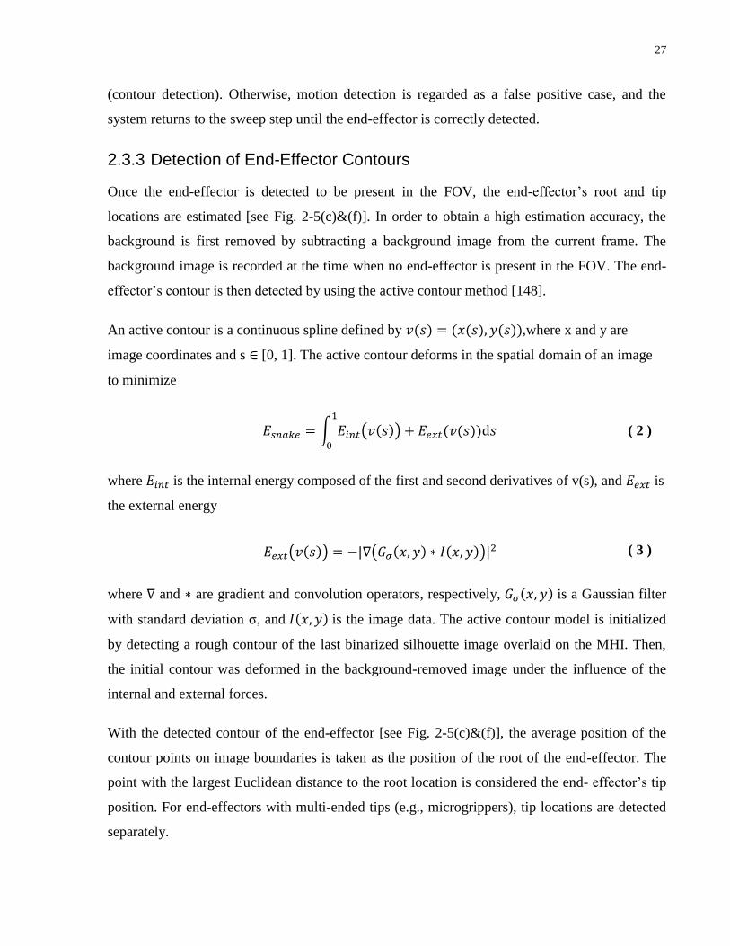
27
(contour detection). Otherwise, motion detection is regarded as a false positive case, and the
system returns to the sweep step until the end-effector is correctly detected.
2.3.3 Detection of End-Effector Contours
Once the end-effector is detected to be present in the FOV, the end-effector‟s root and tip
locations are estimated [see Fig. 2-5(c)&(f)]. In order to obtain a high estimation accuracy, the
background is first removed by subtracting a background image from the current frame. The
background image is recorded at the time when no end-effector is present in the FOV. The end-
effector‟s contour is then detected by using the active contour method [148].
An active contour is a continuous spline defined by ,where x and y are
image coordinates and s ∈ [0, 1]. The active contour deforms in the spatial domain of an image
to minimize
∫ ( )
( 2 )
where is the internal energy composed of the first and second derivatives of v(s), and is
the external energy
( ) ( ) ( 3 )
where and are gradient and convolution operators, respectively, is a Gaussian filter
with standard deviation σ, and is the image data. The active contour model is initialized
by detecting a rough contour of the last binarized silhouette image overlaid on the MHI. Then,
the initial contour was deformed in the background-removed image under the influence of the
internal and external forces.
With the detected contour of the end-effector [see Fig. 2-5(c)&(f)], the average position of the
contour points on image boundaries is taken as the position of the root of the end-effector. The
point with the largest Euclidean distance to the root location is considered the end- effector‟s tip
position. For end-effectors with multi-ended tips (e.g., microgrippers), tip locations are detected
separately.
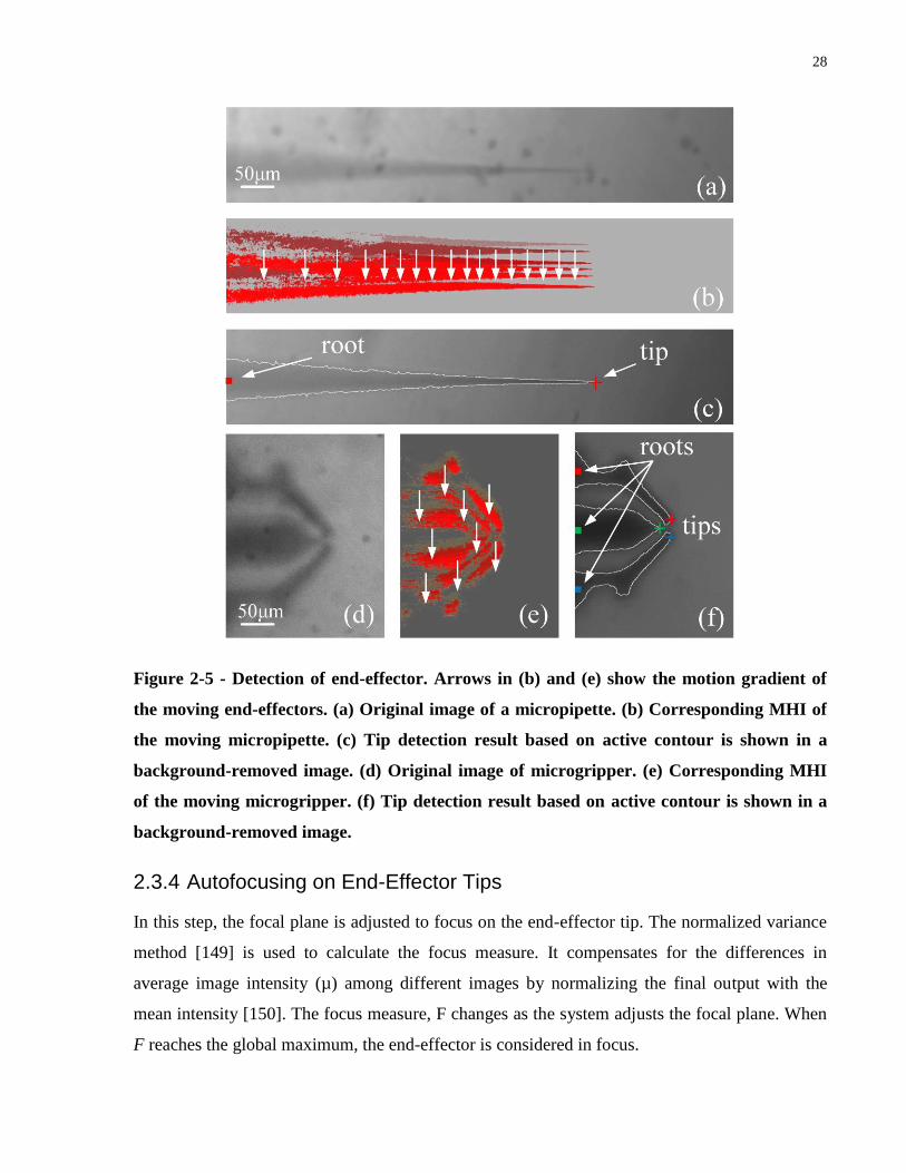
28
Figure 2-5 - Detection of end-effector. Arrows in (b) and (e) show the motion gradient of
the moving end-effectors. (a) Original image of a micropipette. (b) Corresponding MHI of
the moving micropipette. (c) Tip detection result based on active contour is shown in a
background-removed image. (d) Original image of microgripper. (e) Corresponding MHI
of the moving microgripper. (f) Tip detection result based on active contour is shown in a
background-removed image.
2.3.4 Autofocusing on End-Effector Tips
In this step, the focal plane is adjusted to focus on the end-effector tip. The normalized variance
method [149] is used to calculate the focus measure. It compensates for the differences in
average image intensity (µ) among different images by normalizing the final output with the
mean intensity [150]. The focus measure, F changes as the system adjusts the focal plane. When
F reaches the global maximum, the end-effector is considered in focus.
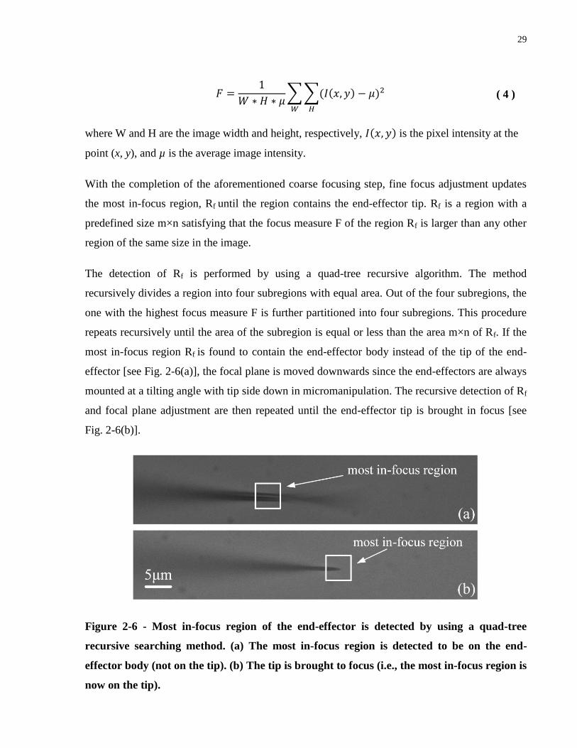
29
∑∑
( 4 )
where W and H are the image width and height, respectively, is the pixel intensity at the
point (x, y), and µ is the average image intensity.
With the completion of the aforementioned coarse focusing step, fine focus adjustment updates
the most in-focus region, Rf until the region contains the end-effector tip. Rf is a region with a
predefined size m×n satisfying that the focus measure F of the region Rf is larger than any other
region of the same size in the image.
The detection of Rf is performed by using a quad-tree recursive algorithm. The method
recursively divides a region into four subregions with equal area. Out of the four subregions, the
one with the highest focus measure F is further partitioned into four subregions. This procedure
repeats recursively until the area of the subregion is equal or less than the area m×n of Rf. If the
most in-focus region Rf is found to contain the end-effector body instead of the tip of the end-
effector [see Fig. 2-6(a)], the focal plane is moved downwards since the end-effectors are always
mounted at a tilting angle with tip side down in micromanipulation. The recursive detection of Rf
and focal plane adjustment are then repeated until the end-effector tip is brought in focus [see
Fig. 2-6(b)].
Figure 2-6 - Most in-focus region of the end-effector is detected by using a quad-tree
recursive searching method. (a) The most in-focus region is detected to be on the end-
effector body (not on the tip). (b) The tip is brought to focus (i.e., the most in-focus region is
now on the tip).
30
2.3.5 Centering End-Effector Tips via Visual Servo Control
After the end-effector tip is brought in focus under a low- magnification objective, centering the
tips is performed before the microscope switches to a higher magnification. By centering the tips
under a low magnification, the end-effector is more likely to be present in the FOV when
switching to a higher magnification. Experimentally, this step can significantly reduce the X–Y
sweeping time required to locate the end-effector under higher magnifications. In the system, the
in-focus end-effector tip is visually tracked and centered via closed- loop visual servo control.
Visual tracking algorithms can be classified into point tracking, kernel tracking, and silhouette
tracking [151]. Representative algorithms were implemented in this study, and their performance
was compared. In point tracking, the center point of the most in-focus region is detected and
taken as the initial end-effector tip position. Since the end-effector was moved at a constant
speed, the motion of end-effector tips was modeled as a constant velocity system. A Kalman
filter is then applied to predict and optimize the end-effector tip position. In the kernel tracking
category, template matching was tested to track end-effector tips. A template is manually
captured, and the normalized cross-correlation [152] of the template with real-time images is
calculated as a measure to detect the end-effector‟s tip. Silhouette tracking is typically based on
contour evolution and shape recognition. The active contour tracking approach was chosen and
tested to detect the end-effector tip within a region of interest. For an end-effector with multi-
ended tips, an average position of all tips was used as the overall tip position. Using the visually
tracked tip position as feedback, an image-based PID visual servo controller was used to position
the end-effector tip to the center of the FOV.
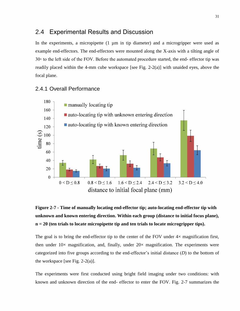
31
2.4 Experimental Results and Discussion
In the experiments, a micropipette (1 µm in tip diameter) and a microgripper were used as
example end-effectors. The end-effectors were mounted along the X-axis with a tilting angle of
30◦ to the left side of the FOV. Before the automated procedure started, the end- effector tip was
readily placed within the 4-mm cube workspace [see Fig. 2-2(a)] with unaided eyes, above the
focal plane.
2.4.1 Overall Performance
Figure 2-7 - Time of manually locating end-effector tip; auto-locating end-effector tip with
unknown and known entering direction. Within each group (distance to initial focus plane),
n = 20 (ten trials to locate micropipette tip and ten trials to locate microgripper tips).
The goal is to bring the end-effector tip to the center of the FOV under 4× magnification first,
then under 10× magnification, and, finally, under 20× magnification. The experiments were
categorized into five groups according to the end-effector‟s initial distance (D) to the bottom of
the workspace [see Fig. 2-2(a)].
The experiments were first conducted using bright field imaging under two conditions: with
known and unknown direction of the end- effector to enter the FOV. Fig. 2-7 summarizes the
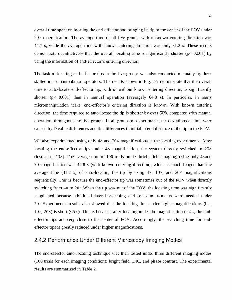
32
overall time spent on locating the end-effector and bringing its tip to the center of the FOV under
20× magnification. The average time of all five groups with unknown entering direction was
44.7 s, while the average time with known entering direction was only 31.2 s. These results
demonstrate quantitatively that the overall locating time is significantly shorter (p< 0.001) by
using the information of end-effector‟s entering direction.
The task of locating end-effector tips in the five groups was also conducted manually by three
skilled micromanipulation operators. The results shown in Fig. 2-7 demonstrate that the overall
time to auto-locate end-effector tip, with or without known entering direction, is significantly
shorter (p< 0.001) than in manual operation (averagely 64.8 s). In particular, in many
micromanipulation tasks, end-effector‟s entering direction is known. With known entering
direction, the time required to auto-locate the tip is shorter by over 50% compared with manual
operation, throughout the five groups. In all groups of experiments, the deviations of time were
caused by D value differences and the differences in initial lateral distance of the tip to the FOV.
We also experimented using only 4× and 20× magnifications in the locating experiments. After
locating the end-effector tips under 4× magnification, the system directly switched to 20×
(instead of 10×). The average time of 100 trials (under bright field imaging) using only 4×and
20×magnificationswas 44.8 s (with known entering direction), which is much longer than the
average time (31.2 s) of auto-locating the tip by using 4×, 10×, and 20× magnifications
sequentially. This is because the end-effector tip was sometimes out of the FOV when directly
switching from 4× to 20×.When the tip was out of the FOV, the locating time was significantly
lengthened because additional lateral sweeping and focus adjustments were needed under
20×.Experimental results also showed that the locating time under higher magnifications (i.e.,
10×, 20×) is short (<5 s). This is because, after locating under the magnification of 4×, the end-
effector tips are very close to the center of FOV. Accordingly, the searching time for end-
effector tips is greatly reduced under higher magnifications.
2.4.2 Performance Under Different Microscopy Imaging Modes
The end-effector auto-locating technique was then tested under three different imaging modes
(100 trials for each imaging condition): bright field, DIC, and phase contrast. The experimental
results are summarized in Table 2.
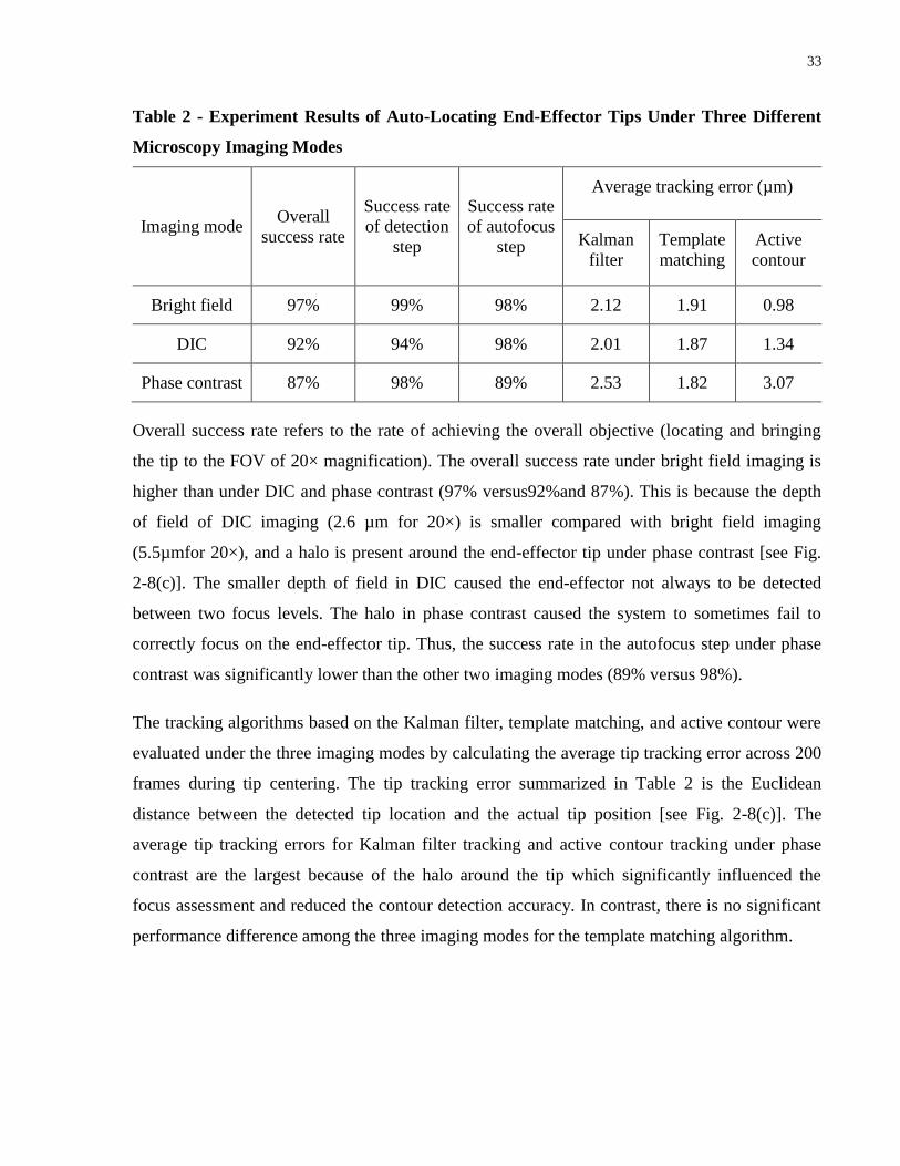
33
Table 2 - Experiment Results of Auto-Locating End-Effector Tips Under Three Different
Microscopy Imaging Modes
Imaging mode Overall
success rate
Success rate
of detection
step
Success rate
of autofocus
step
Average tracking error (µm)
Kalman
filter
Template
matching
Active
contour
Bright field 97% 99% 98% 2.12 1.91 0.98
DIC 92% 94% 98% 2.01 1.87 1.34
Phase contrast 87% 98% 89% 2.53 1.82 3.07
Overall success rate refers to the rate of achieving the overall objective (locating and bringing
the tip to the FOV of 20× magnification). The overall success rate under bright field imaging is
higher than under DIC and phase contrast (97% versus92%and 87%). This is because the depth
of field of DIC imaging (2.6 µm for 20×) is smaller compared with bright field imaging
(5.5µmfor 20×), and a halo is present around the end-effector tip under phase contrast [see Fig.
2-8(c)]. The smaller depth of field in DIC caused the end-effector not always to be detected
between two focus levels. The halo in phase contrast caused the system to sometimes fail to
correctly focus on the end-effector tip. Thus, the success rate in the autofocus step under phase
contrast was significantly lower than the other two imaging modes (89% versus 98%).
The tracking algorithms based on the Kalman filter, template matching, and active contour were
evaluated under the three imaging modes by calculating the average tip tracking error across 200
frames during tip centering. The tip tracking error summarized in Table 2 is the Euclidean
distance between the detected tip location and the actual tip position [see Fig. 2-8(c)]. The
average tip tracking errors for Kalman filter tracking and active contour tracking under phase
contrast are the largest because of the halo around the tip which significantly influenced the
focus assessment and reduced the contour detection accuracy. In contrast, there is no significant
performance difference among the three imaging modes for the template matching algorithm.
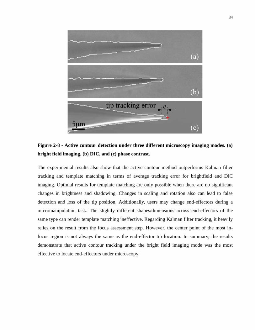
34
Figure 2-8 - Active contour detection under three different microscopy imaging modes. (a)
bright field imaging, (b) DIC, and (c) phase contrast.
The experimental results also show that the active contour method outperforms Kalman filter
tracking and template matching in terms of average tracking error for brightfield and DIC
imaging. Optimal results for template matching are only possible when there are no significant
changes in brightness and shadowing. Changes in scaling and rotation also can lead to false
detection and loss of the tip position. Additionally, users may change end-effectors during a
micromanipulation task. The slightly different shapes/dimensions across end-effectors of the
same type can render template matching ineffective. Regarding Kalman filter tracking, it heavily
relies on the result from the focus assessment step. However, the center point of the most in-
focus region is not always the same as the end-effector tip location. In summary, the results
demonstrate that active contour tracking under the bright field imaging mode was the most
effective to locate end-effectors under microscopy.
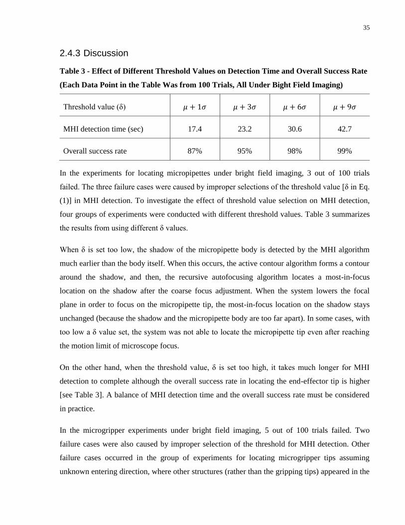
35
2.4.3 Discussion
Table 3 - Effect of Different Threshold Values on Detection Time and Overall Success Rate
(Each Data Point in the Table Was from 100 Trials, All Under Bight Field Imaging)
Threshold value (δ)
MHI detection time (sec) 17.4 23.2 30.6 42.7
Overall success rate 87% 95% 98% 99%
In the experiments for locating micropipettes under bright field imaging, 3 out of 100 trials
failed. The three failure cases were caused by improper selections of the threshold value [δ in Eq.
(1)] in MHI detection. To investigate the effect of threshold value selection on MHI detection,
four groups of experiments were conducted with different threshold values. Table 3 summarizes
the results from using different δ values.
When δ is set too low, the shadow of the micropipette body is detected by the MHI algorithm
much earlier than the body itself. When this occurs, the active contour algorithm forms a contour
around the shadow, and then, the recursive autofocusing algorithm locates a most-in-focus
location on the shadow after the coarse focus adjustment. When the system lowers the focal
plane in order to focus on the micropipette tip, the most-in-focus location on the shadow stays
unchanged (because the shadow and the micropipette body are too far apart). In some cases, with
too low a δ value set, the system was not able to locate the micropipette tip even after reaching
the motion limit of microscope focus.
On the other hand, when the threshold value, δ is set too high, it takes much longer for MHI
detection to complete although the overall success rate in locating the end-effector tip is higher
[see Table 3]. A balance of MHI detection time and the overall success rate must be considered
in practice.
In the microgripper experiments under bright field imaging, 5 out of 100 trials failed. Two
failure cases were also caused by improper selection of the threshold for MHI detection. Other
failure cases occurred in the group of experiments for locating microgripper tips assuming
unknown entering direction, where other structures (rather than the gripping tips) appeared in the
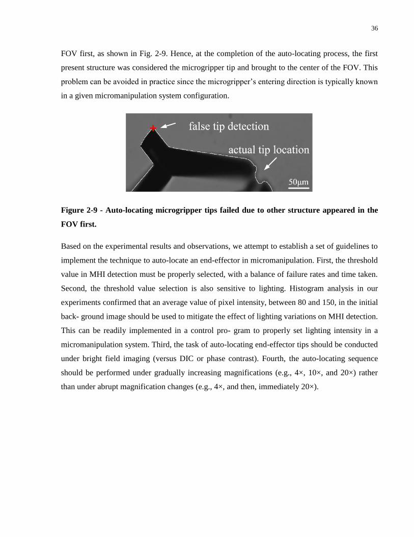
36
FOV first, as shown in Fig. 2-9. Hence, at the completion of the auto-locating process, the first
present structure was considered the microgripper tip and brought to the center of the FOV. This
problem can be avoided in practice since the microgripper‟s entering direction is typically known
in a given micromanipulation system configuration.
Figure 2-9 - Auto-locating microgripper tips failed due to other structure appeared in the
FOV first.
Based on the experimental results and observations, we attempt to establish a set of guidelines to
implement the technique to auto-locate an end-effector in micromanipulation. First, the threshold
value in MHI detection must be properly selected, with a balance of failure rates and time taken.
Second, the threshold value selection is also sensitive to lighting. Histogram analysis in our
experiments confirmed that an average value of pixel intensity, between 80 and 150, in the initial
back- ground image should be used to mitigate the effect of lighting variations on MHI detection.
This can be readily implemented in a control pro- gram to properly set lighting intensity in a
micromanipulation system. Third, the task of auto-locating end-effector tips should be conducted
under bright field imaging (versus DIC or phase contrast). Fourth, the auto-locating sequence
should be performed under gradually increasing magnifications (e.g., 4×, 10×, and 20×) rather
than under abrupt magnification changes (e.g., 4×, and then, immediately 20×).
37
2.5 Conclusion and Guidelines for Implementation
This chapter presented a technique to automatically locate an end-effector under microscopy
imaging. Locating the end-effector tip is the very first step in either manual or automated
micromanipulation. The technique described in this chapter is capable of searching for out-of-
FOV, out-of-focus, and low contrast end-effectors. Experimental results demonstrate that the
search time can be reduced by over 50% with the automated technique. The overall success rate
of the locating system is 97% under the bright field imaging mode. Based on the experimental
results and observations, the following guidelines are established to implement the technique of
auto-locating end-effector tips in order to achieve a high efficiency and success rate.
1. The threshold value in MHI detection must be properly set ([µ + 3σ, µ +6σ]).
2. Lighting intensity must be properly set, for instance, with the average value of pixel
intensity in the initial background image set between 80 and 150.
3. Bright field imaging should be chosen (versus DIC and phase contrast) in the auto-
locating process.
4. The active contour algorithm is most effective under bright field imaging to detect and
track end-effector tips.
5. Abrupt magnification change should be avoided when switching from a low to a high
magnification.
6. The prior knowledge of end-effector entering direction improves both completion time
and the overall success rate.
38
Chapter 3 Robotic Microinjection of Adherent Cells
Compared to robotic injection of suspended cells (e.g., embryos and oocytes), fewer attempts
were made to automate the injection of adherent cells (e.g., cancer cells and cardiomyocytes) due
to their smaller size, highly irregular morphology, small thickness (a few micrometers thick), and
large variations in thickness across cells. This chapter presents a robotic system for automated
microinjection of adherent cells. The system is embedded with several new capabilities:
automatically locating micropipette tips; robustly detecting the contact of micropipette tip with
cell culturing surface and directly with cell membrane; and precisely compensating for
accumulative positioning errors. These new capabilities make it practical to perform adherent
cell microinjection truly via computer mouse clicking in front of a computer monitor, on
hundreds and thousands of cells per experiment (vs. a few to tens of cells as state-of-the-art).
System operation speed, success rate, and cell viability rate were quantitatively evaluated based
on robotic microinjection of over 4,000 cells. This chapter also reports the use of the new robotic
system to perform cell-cell communication studies using large sample sizes. The gap junction
function in a cardiac muscle cell line (HL-1 cells), for the first time, was quantified with the
system.
The following section is based on the text from the following publications:
J. Liu, V. Siragam, Z. Gong, J. Chen, M.D. Fridman, C. Leung, Z. Lu, C.H. Ru, S.R. Xie, J.
Luo, R. Hamilton, and Y. Sun, "Robotic adherent cell injection (RACI) for characterizing cell-
cell communication," IEEE Transactions on Biomedical Engineering, vol. 62, no. 1, pp. 119-24,
2015.
J. Liu, V. Siragam, J. Chen, M.D. Fridman, R.M. Hamilton, and Y. Sun, "High-throughput
measurement of gap junctional intercellular communication," American Journal of Physiology -
Heart and Circulatory Physiology (AJP-Heart), Vol. 306, pp. H1708-13, 2014.
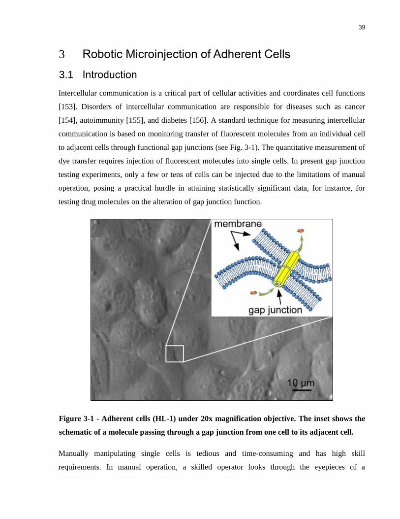
39
Robotic Microinjection of Adherent Cells 3
3.1 Introduction
Intercellular communication is a critical part of cellular activities and coordinates cell functions
[153]. Disorders of intercellular communication are responsible for diseases such as cancer
[154], autoimmunity [155], and diabetes [156]. A standard technique for measuring intercellular
communication is based on monitoring transfer of fluorescent molecules from an individual cell
to adjacent cells through functional gap junctions (see Fig. 3-1). The quantitative measurement of
dye transfer requires injection of fluorescent molecules into single cells. In present gap junction
testing experiments, only a few or tens of cells can be injected due to the limitations of manual
operation, posing a practical hurdle in attaining statistically significant data, for instance, for
testing drug molecules on the alteration of gap junction function.
Figure 3-1 - Adherent cells (HL-1) under 20x magnification objective. The inset shows the
schematic of a molecule passing through a gap junction from one cell to its adjacent cell.
Manually manipulating single cells is tedious and time-consuming and has high skill
requirements. In manual operation, a skilled operator looks through the eyepieces of a
40
microscope while dexterously controlling multiple devices (e.g., micromanipulators, pump,
microscope stage etc.). Robotic cell manipulation technologies progressed significantly over the
past decade. The vast majority of demonstrated robotic systems focused on the manipulation of
suspended cells (i.e., oocytes and embryos) [157]–[162]. Fewer attempts were made to automate
the injection of adherent cells.
Most mammalian cells (e.g., cancer cells and cardiomyocytes) adhere to a culturing surface.
Different from large suspend cells (e.g., mouse oocytes ∼100 µm; zebrafish embryos ∼1 mm),
adherent cells are smaller in size and highly irregular in morphology (vs. spherical for
oocytes/embryos), making robust pattern recognition difficult and automation challenging [163].
Additionally, adherent cells are only a few micrometers thick and vary significantly in thickness,
posing more stringent requirements in robotic positioning.
A few joystick-based systems were demonstrated to assist operators for adherent cell
microinjection [164], [120]. Long training, low success rates, and poor reproducibility make
these systems incapable of injecting more than tens of cells per experiment. For example, the
most popular commercial system for adherent cell injection is Eppendorf‟s InjectMan system that
requires an operator to look into the eyepieces of a microscope and perform microinjection by
controlling joysticks. The injection success rate and cell survival rate of the system are 49.2%
and 49.72%, respectively [164]. The only other joystick-based adherent cell injection system was
demonstrated for the injection of fluorescent molecules into adherent cell lines with a 49%
injection success rate [120]. Due to the difficulty of operating joysticks for fine positioning
control, this system does not permit the injection of a high number of cells (only 82 cells
injected). An automated system integrating a cell detection algorithm reported in [127] produced
a success rate of 67% at a speed of 7-8 cells/minute.
In our previous work in the robotic injection of adherent cells [165], we attempted to transform
joystick-based operation to computer mouse clicking. However, several practical limitations in
the system required the operator to manually perform a few key steps using joysticks and looking
into the eyepieces of the microscope. This hybrid way of system operation (mouse clicking in
front of a computer monitor, and operating joysticks under a microscope) precluded the system‟s
potential for routine use in biology labs. Firstly, the system lacked the critical capability for
automatically locating a micropipette tip. In adherent cell injection, the size of micropipette tip
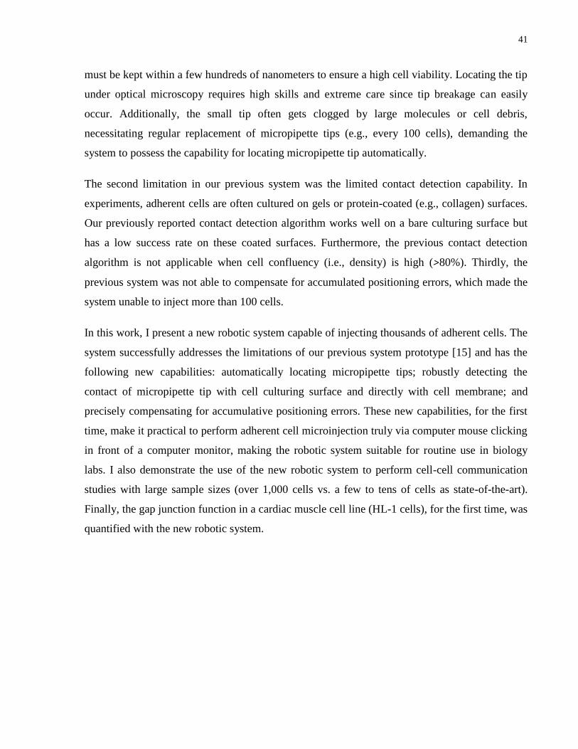
41
must be kept within a few hundreds of nanometers to ensure a high cell viability. Locating the tip
under optical microscopy requires high skills and extreme care since tip breakage can easily
occur. Additionally, the small tip often gets clogged by large molecules or cell debris,
necessitating regular replacement of micropipette tips (e.g., every 100 cells), demanding the
system to possess the capability for locating micropipette tip automatically.
The second limitation in our previous system was the limited contact detection capability. In
experiments, adherent cells are often cultured on gels or protein-coated (e.g., collagen) surfaces.
Our previously reported contact detection algorithm works well on a bare culturing surface but
has a low success rate on these coated surfaces. Furthermore, the previous contact detection
algorithm is not applicable when cell confluency (i.e., density) is high (>80%). Thirdly, the
previous system was not able to compensate for accumulated positioning errors, which made the
system unable to inject more than 100 cells.
In this work, I present a new robotic system capable of injecting thousands of adherent cells. The
system successfully addresses the limitations of our previous system prototype [15] and has the
following new capabilities: automatically locating micropipette tips; robustly detecting the
contact of micropipette tip with cell culturing surface and directly with cell membrane; and
precisely compensating for accumulative positioning errors. These new capabilities, for the first
time, make it practical to perform adherent cell microinjection truly via computer mouse clicking
in front of a computer monitor, making the robotic system suitable for routine use in biology
labs. I also demonstrate the use of the new robotic system to perform cell-cell communication
studies with large sample sizes (over 1,000 cells vs. a few to tens of cells as state-of-the-art).
Finally, the gap junction function in a cardiac muscle cell line (HL-1 cells), for the first time, was
quantified with the new robotic system.
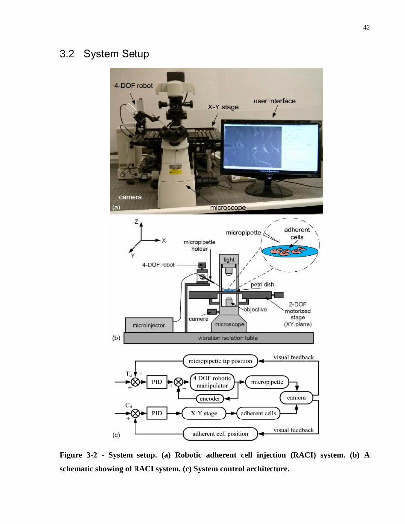
42
3.2 System Setup
Figure 3-2 - System setup. (a) Robotic adherent cell injection (RACI) system. (b) A
schematic showing of RACI system. (c) System control architecture.
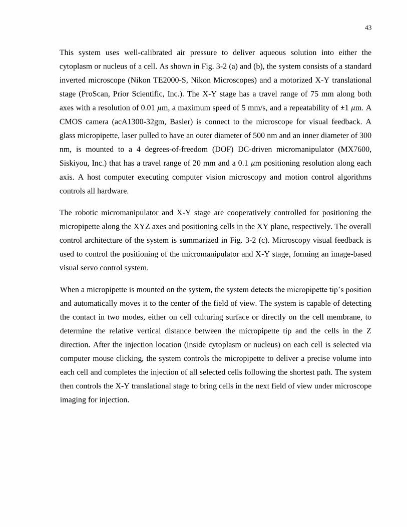
43
This system uses well-calibrated air pressure to deliver aqueous solution into either the
cytoplasm or nucleus of a cell. As shown in Fig. 3-2 (a) and (b), the system consists of a standard
inverted microscope (Nikon TE2000-S, Nikon Microscopes) and a motorized X-Y translational
stage (ProScan, Prior Scientific, Inc.). The X-Y stage has a travel range of 75 mm along both
axes with a resolution of 0.01 µm, a maximum speed of 5 mm/s, and a repeatability of ±1 µm. A
CMOS camera (acA1300-32gm, Basler) is connect to the microscope for visual feedback. A
glass micropipette, laser pulled to have an outer diameter of 500 nm and an inner diameter of 300
nm, is mounted to a 4 degrees-of-freedom (DOF) DC-driven micromanipulator (MX7600,
Siskiyou, Inc.) that has a travel range of 20 mm and a 0.1 µm positioning resolution along each
axis. A host computer executing computer vision microscopy and motion control algorithms
controls all hardware.
The robotic micromanipulator and X-Y stage are cooperatively controlled for positioning the
micropipette along the XYZ axes and positioning cells in the XY plane, respectively. The overall
control architecture of the system is summarized in Fig. 3-2 (c). Microscopy visual feedback is
used to control the positioning of the micromanipulator and X-Y stage, forming an image-based
visual servo control system.
When a micropipette is mounted on the system, the system detects the micropipette tip‟s position
and automatically moves it to the center of the field of view. The system is capable of detecting
the contact in two modes, either on cell culturing surface or directly on the cell membrane, to
determine the relative vertical distance between the micropipette tip and the cells in the Z
direction. After the injection location (inside cytoplasm or nucleus) on each cell is selected via
computer mouse clicking, the system controls the micropipette to deliver a precise volume into
each cell and completes the injection of all selected cells following the shortest path. The system
then controls the X-Y translational stage to bring cells in the next field of view under microscope
imaging for injection.
44
3.3 Vision Based Contact Detection
3.3.1 Contact Detection on Cell Culture Surface
Figure 3-3 - Contact detection on cell culture surface. (a) Micropipette tip is lowered
towards the cell culture surface while the X-Y stage moves along the X-axis from left to
right. (b) Micropipette tip slides horizontally when it contacts the culture surface. (c)
Schematic showing micropipette is lowered towards cell culture surface. (d) Schematic
showing micropipette tip is sliding along the X-axis.
In order to inject materials into a cell, the relative vertical distance between the micropipette tip
and the cell along the Z-direction must be accurately detected. Without the inclusion of an extra
sensor (e.g., tactile or force sensors), which increases hardware complexity, two modes of
computer vision based contact detection algorithms are developed to accurately determine the
relative heights of the micropipette tip and adherent cells. This section describes the first mode,
in which the system detects the initial contact of micropipette tip on the cell culturing surface that
is protein coated (vs. bare surface).
Empty Region Detection: When cell confluency is lower than 80%, empty areas on the
culturing surface can be detected and used for contact detection. The system divides the field of
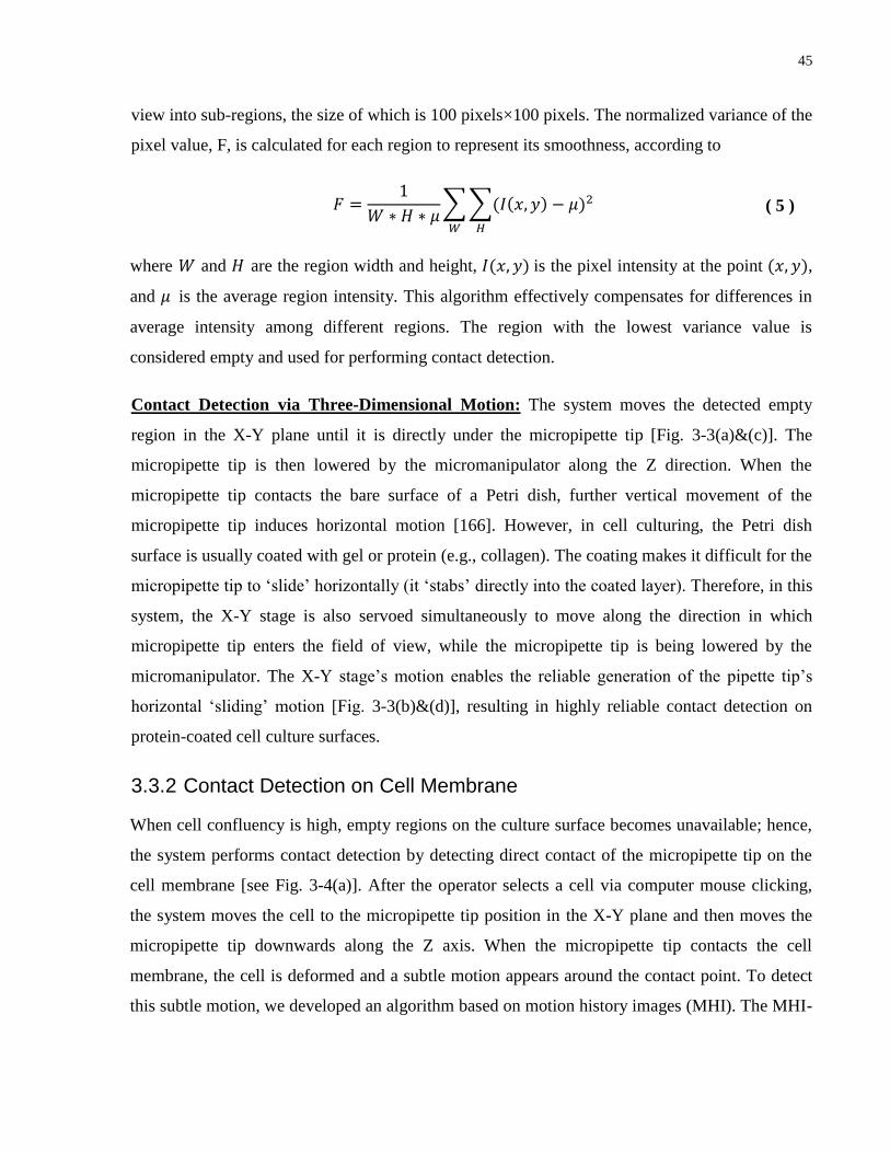
45
view into sub-regions, the size of which is 100 pixels×100 pixels. The normalized variance of the
pixel value, F, is calculated for each region to represent its smoothness, according to
∑∑
( 5 )
where W and H are the region width and height, is the pixel intensity at the point ,
and µ is the average region intensity. This algorithm effectively compensates for differences in
average intensity among different regions. The region with the lowest variance value is
considered empty and used for performing contact detection.
Contact Detection via Three-Dimensional Motion: The system moves the detected empty
region in the X-Y plane until it is directly under the micropipette tip [Fig. 3-3(a)&(c)]. The
micropipette tip is then lowered by the micromanipulator along the Z direction. When the
micropipette tip contacts the bare surface of a Petri dish, further vertical movement of the
micropipette tip induces horizontal motion [166]. However, in cell culturing, the Petri dish
surface is usually coated with gel or protein (e.g., collagen). The coating makes it difficult for the
micropipette tip to „slide‟ horizontally (it „stabs‟ directly into the coated layer). Therefore, in this
system, the X-Y stage is also servoed simultaneously to move along the direction in which
micropipette tip enters the field of view, while the micropipette tip is being lowered by the
micromanipulator. The X-Y stage‟s motion enables the reliable generation of the pipette tip‟s
horizontal „sliding‟ motion [Fig. 3-3(b)&(d)], resulting in highly reliable contact detection on
protein-coated cell culture surfaces.
3.3.2 Contact Detection on Cell Membrane
When cell confluency is high, empty regions on the culture surface becomes unavailable; hence,
the system performs contact detection by detecting direct contact of the micropipette tip on the
cell membrane [see Fig. 3-4(a)]. After the operator selects a cell via computer mouse clicking,
the system moves the cell to the micropipette tip position in the X-Y plane and then moves the
micropipette tip downwards along the Z axis. When the micropipette tip contacts the cell
membrane, the cell is deformed and a subtle motion appears around the contact point. To detect
this subtle motion, we developed an algorithm based on motion history images (MHI). The MHI-
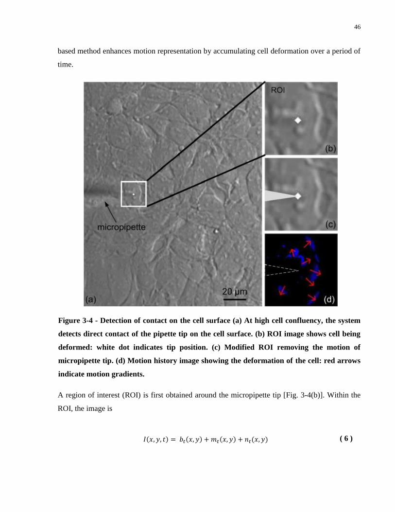
46
based method enhances motion representation by accumulating cell deformation over a period of
time.
Figure 3-4 - Detection of contact on the cell surface (a) At high cell confluency, the system
detects direct contact of the pipette tip on the cell surface. (b) ROI image shows cell being
deformed: white dot indicates tip position. (c) Modified ROI removing the motion of
micropipette tip. (d) Motion history image showing the deformation of the cell: red arrows
indicate motion gradients.
A region of interest (ROI) is first obtained around the micropipette tip [Fig. 3-4(b)]. Within the
ROI, the image is
( 6 )
47
where is the static background; is the moving object; is the background
noise; and is time. The moving object is extracted via taking the difference between
consecutive frames.
( 7 )
where is the motion region; is noise; and is the difference image
containing the moving object and background aberration due to motion and noise. Background
aberration can lead to incorrect detection (e.g., motion ambiguity and distortion) and make
detection fail when object motion speed is low.
In the system, the motion region contains motion from both the lowering micropipette
and cell deformation due to micropipette-and-cell contact. Hence,
( 8 )
where is the micropipette lowering motion, and is the motion from cell
deformation. When the micropipette is moved along Z axis during contact detection, the tip‟s
location in the X-Y plane, , is constant, and the lowering motion results from the
defocusing phenomenon. Since a defocusing blurred image is equivalent to an exponential decay
function [167], the micropipette lowering motion can be described as
( ) , where ( ) is the initial micropipette‟s motion before cell contact
occurs. Thus, motion from cell deformation is
( ) ( 9 )
After removing micropipette tip‟s motion, the noise term in the difference image can
be removed by a Gaussian low-pass filter and image binarization. The binary image representing
cell deformation-caused motion is
{
( 10 )
48
The motion history image is
{
( 11 )
where the duration τ determines the temporal extent of the movement, and γ is the decay
parameter. The subtle cell deforming motion is greatly enhanced by adding the motion history
information [see Fig. 3-4(d)].
The sum of pixel values in MHI, , is calculated as a measure to determine the contact of cell
membrane. If is above a threshold value δ, the micropipette tip is considered as contacting
cell top membrane. The threshold δ is calculated dynamically by analyzing MHIs in which the
micropipette tip has not contacted cell surface.
( 12 )
where is the average of MHIs‟ sum of pixel values before cell contact occurs; is the
standard deviation; and a is a preset parameter which is experimentally determined. By adding
to the mean value, the threshold δ effectively rejects those MHIs that do not contain cell
deformation. In addition, the motion gradient of the MHI is also used to avoid false positive
detection. The motion gradient is computed by convolution with Sobel filters to yield spatial
derivatives, and . The orientation of the motion gradient at each pixel is
( 13 )
As the micropipette tip touches the cell membrane, deformation occurs around the contact point.
Accordingly, the motion gradients in MHI converge to the contact point.
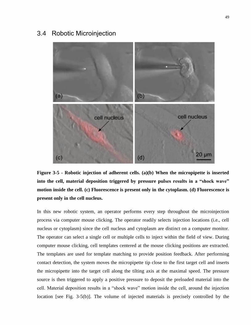
49
3.4 Robotic Microinjection
Figure 3-5 - Robotic injection of adherent cells. (a)(b) When the micropipette is inserted
into the cell, material deposition triggered by pressure pulses results in a “shock wave”
motion inside the cell. (c) Fluorescence is present only in the cytoplasm. (d) Fluorescence is
present only in the cell nucleus.
In this new robotic system, an operator performs every step throughout the microinjection
process via computer mouse clicking. The operator readily selects injection locations (i.e., cell
nucleus or cytoplasm) since the cell nucleus and cytoplasm are distinct on a computer monitor.
The operator can select a single cell or multiple cells to inject within the field of view. During
computer mouse clicking, cell templates centered at the mouse clicking positions are extracted.
The templates are used for template matching to provide position feedback. After performing
contact detection, the system moves the micropipette tip close to the first target cell and inserts
the micropipette into the target cell along the tilting axis at the maximal speed. The pressure
source is then triggered to apply a positive pressure to deposit the preloaded material into the
cell. Material deposition results in a “shock wave” motion inside the cell, around the injection
location [see Fig. 3-5(b)]. The volume of injected materials is precisely controlled by the
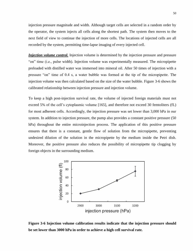
50
injection pressure magnitude and width. Although target cells are selected in a random order by
the operator, the system injects all cells along the shortest path. The system then moves to the
next field of view to continue the injection of more cells. The locations of injected cells are all
recorded by the system, permitting time-lapse imaging of every injected cell.
Injection volume control. Injection volume is determined by the injection pressure and pressure
“on” time (i.e., pulse width). Injection volume was experimentally measured. The micropipette
preloaded with distilled water was immersed into mineral oil. After 50 times of injection with a
pressure “on” time of 0.4 s, a water bubble was formed at the tip of the micropipette. The
injection volume was then calculated based on the size of the water bubble. Figure 3-6 shows the
calibrated relationship between injection pressure and injection volume.
To keep a high post-injection survival rate, the volume of injected foreign materials must not
exceed 5% of the cell‟s cytoplasmic volume [165], and therefore not exceed 30 femtoliters (fL)
for most adherent cells. Accordingly, the injection pressure was set lower than 3,000 hPa in our
system. In addition to injection pressure, the pump also provides a constant positive pressure (50
hPa) throughout the entire microinjection process. The application of this positive pressure
ensures that there is a constant, gentle flow of solution from the micropipette, preventing
undesired dilution of the solution in the micropipette by the medium inside the Petri dish.
Moreover, the positive pressure also reduces the possibility of micropipette tip clogging by
foreign objects in the surrounding medium.
Figure 3-6 Injection volume calibration results indicate that the injection pressure should
be set lower than 3000 hPa in order to achieve a high cell survival rate.
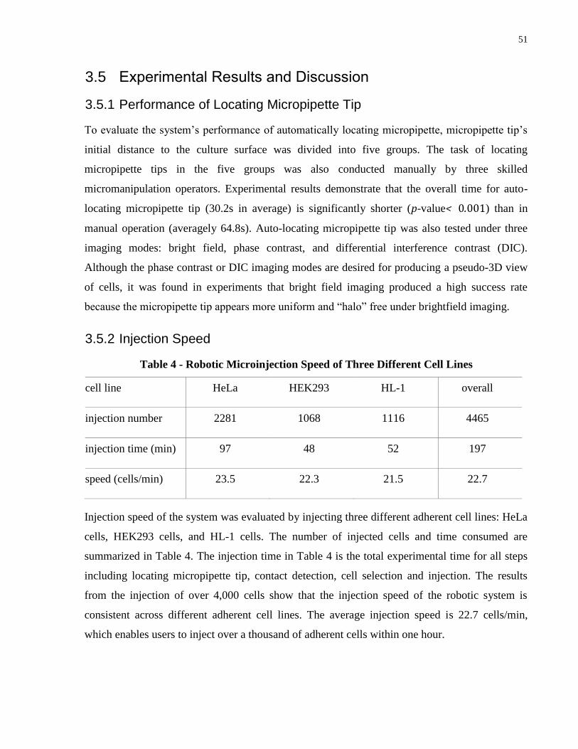
51
3.5 Experimental Results and Discussion
3.5.1 Performance of Locating Micropipette Tip
To evaluate the system‟s performance of automatically locating micropipette, micropipette tip‟s
initial distance to the culture surface was divided into five groups. The task of locating
micropipette tips in the five groups was also conducted manually by three skilled
micromanipulation operators. Experimental results demonstrate that the overall time for auto-
locating micropipette tip (30.2s in average) is significantly shorter (p-value< 0.001) than in
manual operation (averagely 64.8s). Auto-locating micropipette tip was also tested under three
imaging modes: bright field, phase contrast, and differential interference contrast (DIC).
Although the phase contrast or DIC imaging modes are desired for producing a pseudo-3D view
of cells, it was found in experiments that bright field imaging produced a high success rate
because the micropipette tip appears more uniform and “halo” free under brightfield imaging.
3.5.2 Injection Speed
Table 4 - Robotic Microinjection Speed of Three Different Cell Lines
cell line HeLa HEK293 HL-1 overall
injection number 2281 1068 1116 4465
injection time (min) 97 48 52 197
speed (cells/min) 23.5 22.3 21.5 22.7
Injection speed of the system was evaluated by injecting three different adherent cell lines: HeLa
cells, HEK293 cells, and HL-1 cells. The number of injected cells and time consumed are
summarized in Table 4. The injection time in Table 4 is the total experimental time for all steps
including locating micropipette tip, contact detection, cell selection and injection. The results
from the injection of over 4,000 cells show that the injection speed of the robotic system is
consistent across different adherent cell lines. The average injection speed is 22.7 cells/min,
which enables users to inject over a thousand of adherent cells within one hour.
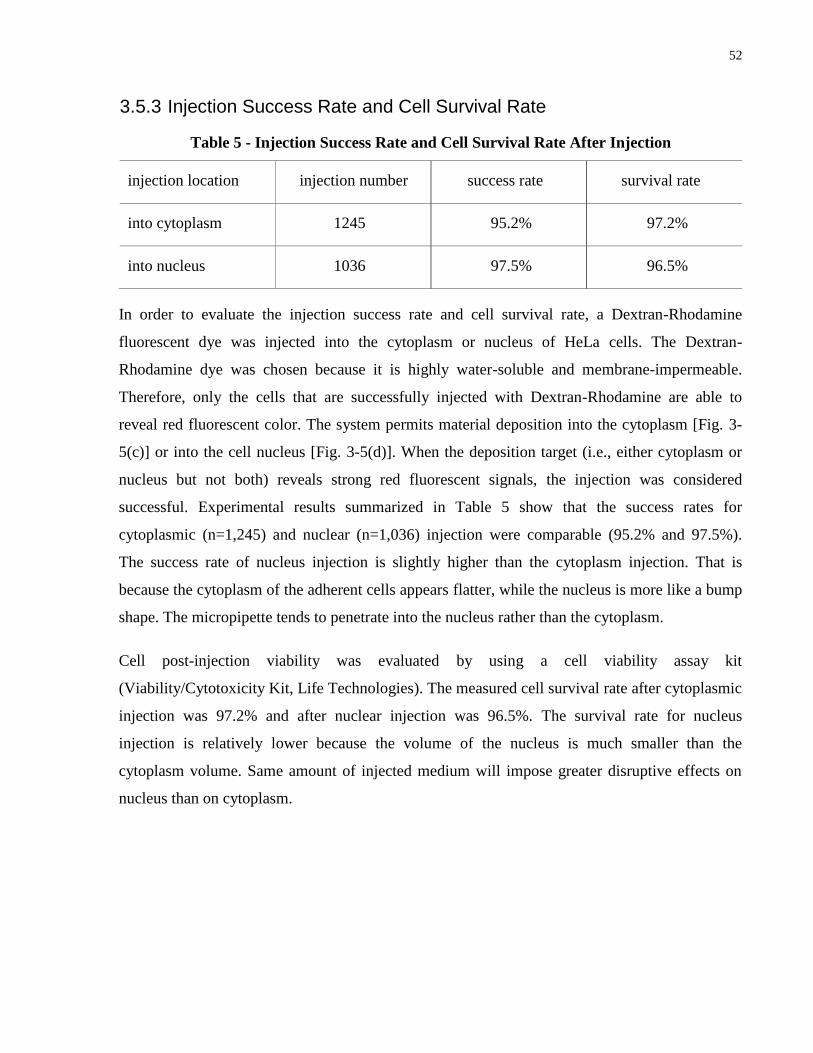
52
3.5.3 Injection Success Rate and Cell Survival Rate
Table 5 - Injection Success Rate and Cell Survival Rate After Injection
injection location injection number success rate survival rate
into cytoplasm 1245 95.2% 97.2%
into nucleus 1036 97.5% 96.5%
In order to evaluate the injection success rate and cell survival rate, a Dextran-Rhodamine
fluorescent dye was injected into the cytoplasm or nucleus of HeLa cells. The Dextran-
Rhodamine dye was chosen because it is highly water-soluble and membrane-impermeable.
Therefore, only the cells that are successfully injected with Dextran-Rhodamine are able to
reveal red fluorescent color. The system permits material deposition into the cytoplasm [Fig. 3-
5(c)] or into the cell nucleus [Fig. 3-5(d)]. When the deposition target (i.e., either cytoplasm or
nucleus but not both) reveals strong red fluorescent signals, the injection was considered
successful. Experimental results summarized in Table 5 show that the success rates for
cytoplasmic (n=1,245) and nuclear (n=1,036) injection were comparable (95.2% and 97.5%).
The success rate of nucleus injection is slightly higher than the cytoplasm injection. That is
because the cytoplasm of the adherent cells appears flatter, while the nucleus is more like a bump
shape. The micropipette tends to penetrate into the nucleus rather than the cytoplasm.
Cell post-injection viability was evaluated by using a cell viability assay kit
(Viability/Cytotoxicity Kit, Life Technologies). The measured cell survival rate after cytoplasmic
injection was 97.2% and after nuclear injection was 96.5%. The survival rate for nucleus
injection is relatively lower because the volume of the nucleus is much smaller than the
cytoplasm volume. Same amount of injected medium will impose greater disruptive effects on
nucleus than on cytoplasm.
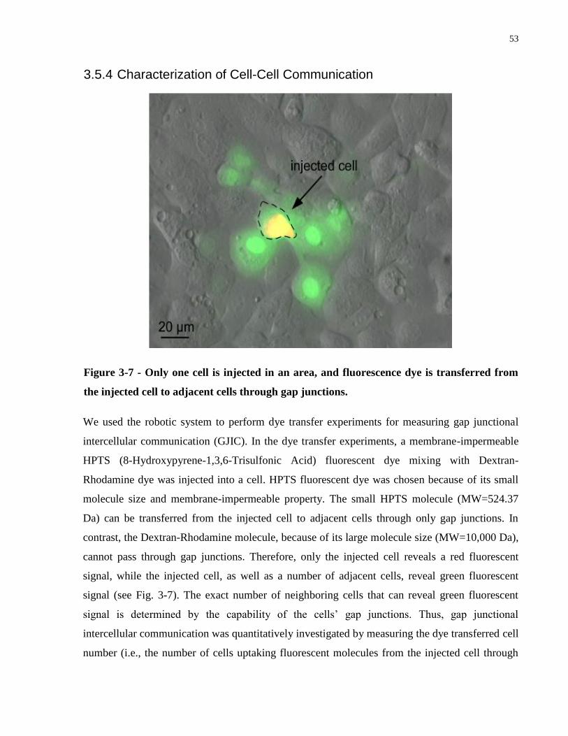
53
3.5.4 Characterization of Cell-Cell Communication
Figure 3-7 - Only one cell is injected in an area, and fluorescence dye is transferred from
the injected cell to adjacent cells through gap junctions.
We used the robotic system to perform dye transfer experiments for measuring gap junctional
intercellular communication (GJIC). In the dye transfer experiments, a membrane-impermeable
HPTS (8-Hydroxypyrene-1,3,6-Trisulfonic Acid) fluorescent dye mixing with Dextran-
Rhodamine dye was injected into a cell. HPTS fluorescent dye was chosen because of its small
molecule size and membrane-impermeable property. The small HPTS molecule (MW=524.37
Da) can be transferred from the injected cell to adjacent cells through only gap junctions. In
contrast, the Dextran-Rhodamine molecule, because of its large molecule size (MW=10,000 Da),
cannot pass through gap junctions. Therefore, only the injected cell reveals a red fluorescent
signal, while the injected cell, as well as a number of adjacent cells, reveal green fluorescent
signal (see Fig. 3-7). The exact number of neighboring cells that can reveal green fluorescent
signal is determined by the capability of the cells‟ gap junctions. Thus, gap junctional
intercellular communication was quantitatively investigated by measuring the dye transferred cell
number (i.e., the number of cells uptaking fluorescent molecules from the injected cell through
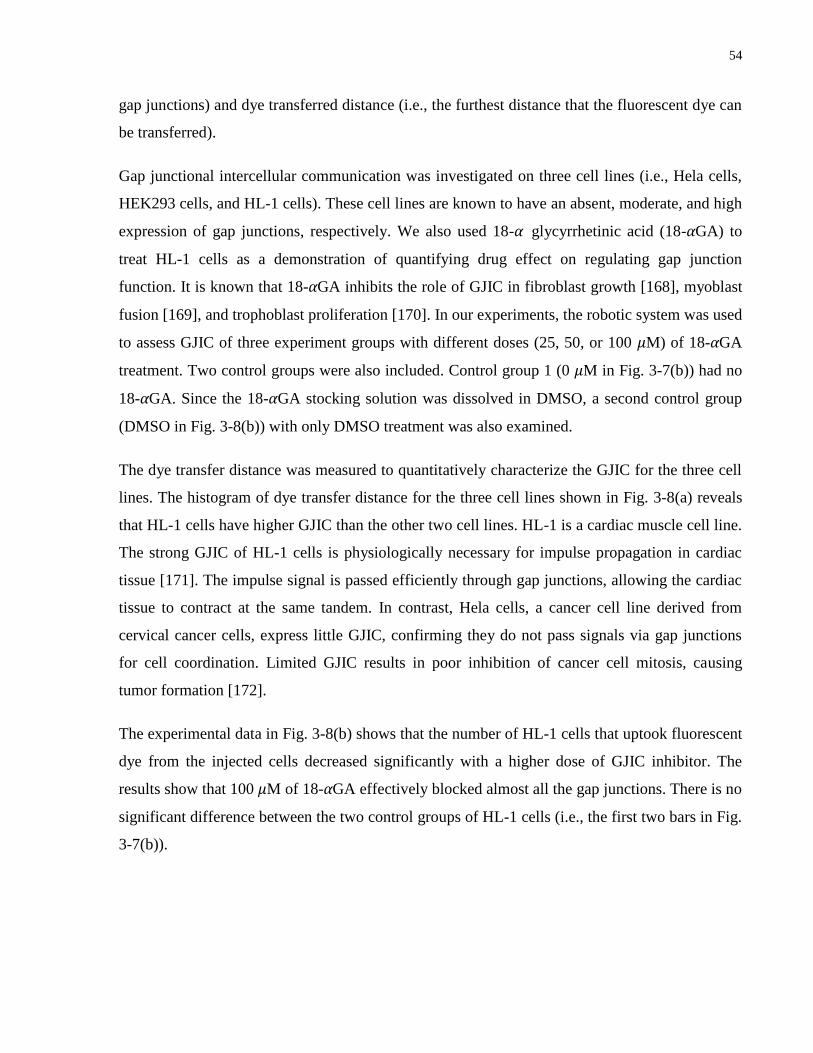
54
gap junctions) and dye transferred distance (i.e., the furthest distance that the fluorescent dye can
be transferred).
Gap junctional intercellular communication was investigated on three cell lines (i.e., Hela cells,
HEK293 cells, and HL-1 cells). These cell lines are known to have an absent, moderate, and high
expression of gap junctions, respectively. We also used 18-α glycyrrhetinic acid (18-αGA) to
treat HL-1 cells as a demonstration of quantifying drug effect on regulating gap junction
function. It is known that 18-αGA inhibits the role of GJIC in fibroblast growth [168], myoblast
fusion [169], and trophoblast proliferation [170]. In our experiments, the robotic system was used
to assess GJIC of three experiment groups with different doses (25, 50, or 100 µM) of 18-αGA
treatment. Two control groups were also included. Control group 1 (0 µM in Fig. 3-7(b)) had no
18-αGA. Since the 18-αGA stocking solution was dissolved in DMSO, a second control group
(DMSO in Fig. 3-8(b)) with only DMSO treatment was also examined.
The dye transfer distance was measured to quantitatively characterize the GJIC for the three cell
lines. The histogram of dye transfer distance for the three cell lines shown in Fig. 3-8(a) reveals
that HL-1 cells have higher GJIC than the other two cell lines. HL-1 is a cardiac muscle cell line.
The strong GJIC of HL-1 cells is physiologically necessary for impulse propagation in cardiac
tissue [171]. The impulse signal is passed efficiently through gap junctions, allowing the cardiac
tissue to contract at the same tandem. In contrast, Hela cells, a cancer cell line derived from
cervical cancer cells, express little GJIC, confirming they do not pass signals via gap junctions
for cell coordination. Limited GJIC results in poor inhibition of cancer cell mitosis, causing
tumor formation [172].
The experimental data in Fig. 3-8(b) shows that the number of HL-1 cells that uptook fluorescent
dye from the injected cells decreased significantly with a higher dose of GJIC inhibitor. The
results show that 100 µM of 18-αGA effectively blocked almost all the gap junctions. There is no
significant difference between the two control groups of HL-1 cells (i.e., the first two bars in Fig.
3-7(b)).
55
Figure 3-8 - Results of dye transfer experiments. (a) Histogram of dye transfer distance for
HeLa cells (n = 200), HEK293 cells (n = 200), and HL-1 cells (n = 400). (b) The number of
HL-1 cells uptaking fluorescence dye from the injected cells. Over 200 cells were injected
for each group.
56
3.5.5 Discussion
Microinjection of adherent cells permits the direct insertion of foreign materials (e.g.,
DNA/RNA, fluorescent dyes, quantum dots etc.) into single cells. It is a decades-old technology
that is still widely used in cell biology for testing cell-cell communication, studying intracellular
behavior, and gene transfection [173].
Manual microinjection of adherent cells and existing robotic system prototypes are limited to the
injection of a few to tens of cells per experiment at best. This new robotic system described in
this chapter is the first system capable of performing microinjection on hundreds and thousands
of cells per experiment. The system is embedded with strong automation capabilities in every
step of operation, enabling an operator to perform the entire microinjection process via mouse
clicking in front of a computer monitor. Training of a user with no skills in microinjection takes
10-15 minutes, and after a few hours‟ operation, the user becomes highly proficient at operating
the system to perform adherent cell microinjection with high success rates.
3.6 Conclusion
This chapter described a robotic adherent cell injection system equipped with several key
technologies that were recently developed. These new techniques include automatically locating
micropipette tips, robustly detecting the contact of micropipette tip with cell culture surface and
directly with the cell membrane, and precisely compensating for accumulative positioning errors.
The high degree of automation of the system enables users with no microinjection training to
perform large-scale cell injection with high success rates. System operation speed, success rate,
and cell viability rate were quantitatively evaluated. Dye transfer experiments were conducted on
different cell lines to establish a powerful assay for characterizing cell gap junction functions.
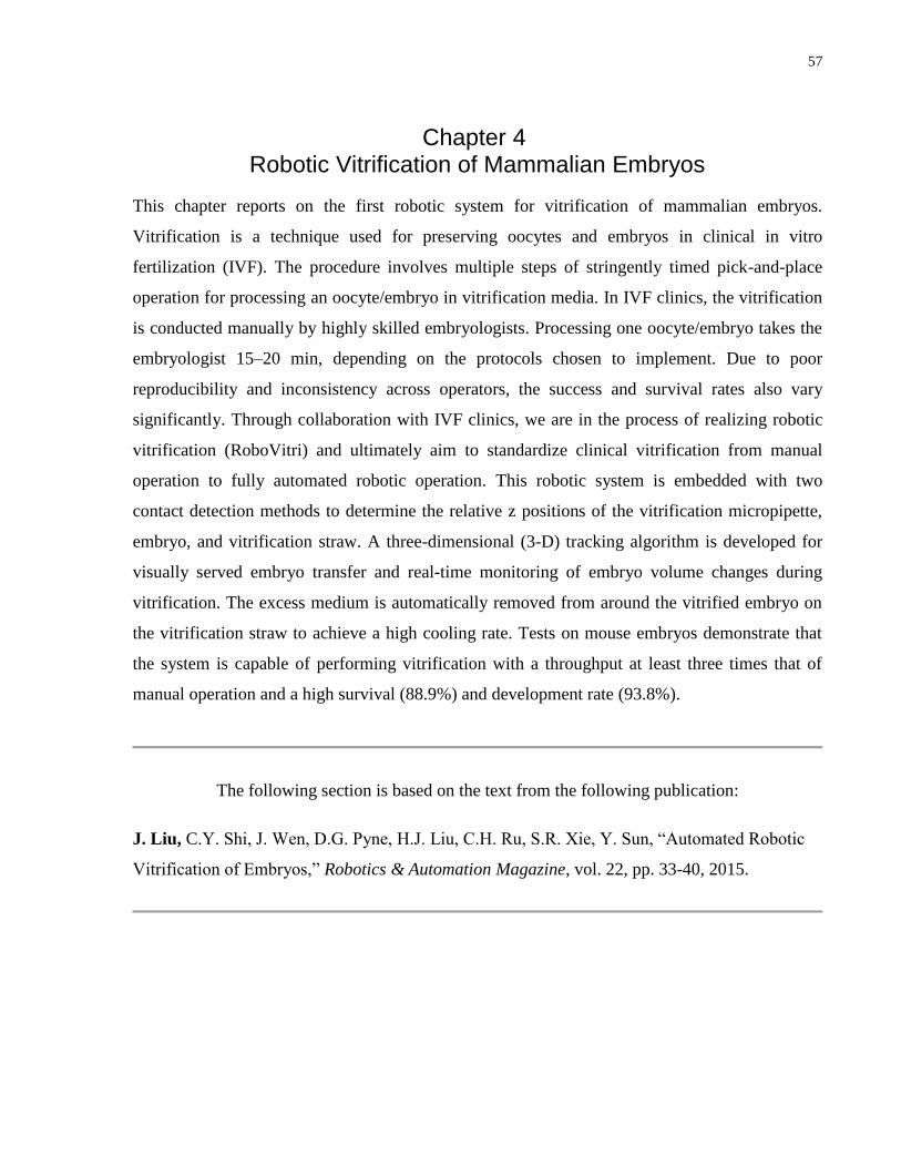
57
Chapter 4 Robotic Vitrification of Mammalian Embryos
This chapter reports on the first robotic system for vitrification of mammalian embryos.
Vitrification is a technique used for preserving oocytes and embryos in clinical in vitro
fertilization (IVF). The procedure involves multiple steps of stringently timed pick-and-place
operation for processing an oocyte/embryo in vitrification media. In IVF clinics, the vitrification
is conducted manually by highly skilled embryologists. Processing one oocyte/embryo takes the
embryologist 15–20 min, depending on the protocols chosen to implement. Due to poor
reproducibility and inconsistency across operators, the success and survival rates also vary
significantly. Through collaboration with IVF clinics, we are in the process of realizing robotic
vitrification (RoboVitri) and ultimately aim to standardize clinical vitrification from manual
operation to fully automated robotic operation. This robotic system is embedded with two
contact detection methods to determine the relative z positions of the vitrification micropipette,
embryo, and vitrification straw. A three-dimensional (3-D) tracking algorithm is developed for
visually served embryo transfer and real-time monitoring of embryo volume changes during
vitrification. The excess medium is automatically removed from around the vitrified embryo on
the vitrification straw to achieve a high cooling rate. Tests on mouse embryos demonstrate that
the system is capable of performing vitrification with a throughput at least three times that of
manual operation and a high survival (88.9%) and development rate (93.8%).
The following section is based on the text from the following publication:
J. Liu, C.Y. Shi, J. Wen, D.G. Pyne, H.J. Liu, C.H. Ru, S.R. Xie, Y. Sun, “Automated Robotic
Vitrification of Embryos,” Robotics & Automation Magazine, vol. 22, pp. 33-40, 2015.
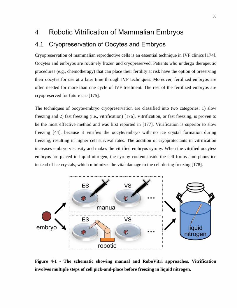
58
Robotic Vitrification of Mammalian Embryos 4
4.1 Cryopreservation of Oocytes and Embryos
Cryopreservation of mammalian reproductive cells is an essential technique in IVF clinics [174].
Oocytes and embryos are routinely frozen and cryopreserved. Patients who undergo therapeutic
procedures (e.g., chemotherapy) that can place their fertility at risk have the option of preserving
their oocytes for use at a later time through IVF techniques. Moreover, fertilized embryos are
often needed for more than one cycle of IVF treatment. The rest of the fertilized embryos are
cryopreserved for future use [175].
The techniques of oocyte/embryo cryopreservation are classified into two categories: 1) slow
freezing and 2) fast freezing (i.e., vitrification) [176]. Vitrification, or fast freezing, is proven to
be the most effective method and was first reported in [177]. Vitrification is superior to slow
freezing [44], because it vitrifies the oocyte/embryo with no ice crystal formation during
freezing, resulting in higher cell survival rates. The addition of cryoprotectants in vitrification
increases embryo viscosity and makes the vitrified embryos syrupy. When the vitrified oocytes/
embryos are placed in liquid nitrogen, the syrupy content inside the cell forms amorphous ice
instead of ice crystals, which minimizes the vital damage to the cell during freezing [178].
Figure 4-1 - The schematic showing manual and RoboVitri approaches. Vitrification
involves multiple steps of cell pick-and-place before freezing in liquid nitrogen.
59
At present, oocyte/embryo vitrification is done manually in IVF clinics globally. An operator
looks through the microscope eyepieces and manipulates oocytes/embryos using a micropipette.
An oocyte/embryo is first picked up and removed from the culture dish and washed with the
equilibrium solution (ES) and a series of vitrification solutions (VSs), as shown in Fig. 4-1.
Within each step, timing control has been proven critical. After the many pick-and-place steps,
the processed oocyte/embryo is placed onto a device called a vitrification straw. The volume of
solution remaining around the oocyte/embryo on the straw must be minimal to ensure a high
cooling rate [179]. The vitrification straw is then plunged into liquid nitrogen for freezing and
long-term cryopreservation. Several commercial the VSs and protocols exist; however, their core
steps are largely the same. All the protocols involve multiple washing steps with the ES and the
VS, placing the vitrified oocytes/embryos on vitrification straws, and freezing the vitrification
straws in liquid nitrogen. Manual oocyte/embryo vitrification is a laborious and demanding task
due to the following reasons.
There is a long learning curve, and intense focus is required for embryologists performing
the manual method.
The anti-freezing solutes [e.g., dimethyl sulfoxide (DMSO)] are toxic to
oocytes/embryos. Therefore, the washing time in the VS is critical but can be difficult to
strictly control by an operator.
Because of their small size (~100 µm), oocytes/embryos can be difficult to detect and
manipulate, especially when the medium surrounding the cells is dynamically changing
(e.g., in viscosity) during micropipette aspiration and dispensing.
The manual process has stringent skill requirements, and the success rate and cell
survival rate can vary significantly across operators.
Over the past few decades, the robotics community has made significant progress in
assisting/standardizing clinical procedures, from the transformative da Vinci surgical system to
robotic systems under intensive development for manipulating single cells [180][181]. To realize
RoboVitri for clinical use, a number of tasks must be tackled with clinically acceptable
reliability, for instance, robust embryo tracking in three dimensions in media of different
viscosities and autonomous transfer of processed embryos from liquid environments to the solid
60
vitrification straw tip. Furthermore, timing control in vitrification is much more stringent and
critical than other cell manipulation tasks (e.g., intracytoplasmic sperm injection [157]) to
achieve high cell development rates after embryo thawing.
Although automated vitrification was attempted using microfluidic approaches [72], [182],
[183], embryo loss is a concern because of difficulties in loading and retrieving embryos onto
and from the microfluidic devices. No attempt has been made to automate vitrification using a
robotic approach.
In this chapter, I present a robotic system prototype for automated vitrification and thawing of
embryos. The system has successfully addressed the major challenges in manual operation with
the following technologies:
(1) automated locating of micropipette and vitrification straws;
(2) contact detection methods to determine the relative z-position of the micropipette tip;
(3) autonomous detection and tracking of embryos in three dimensions;
(4) robotically placing vitrified embryos onto vitrification straws and removing excess medium.
These core techniques make it practical to perform automated RoboVitri of embryos. The
experimental results also demonstrate that the embryo survival and development rates after
vitrification and thawing achieved by the robotic system were higher than those of the manual
group. Automated vitrification would free up embryologists to focus on other tasks in IVF clinics
and provide consistently high success and survival rates. With a higher throughput, automated
vitrification also has the potential to become a standard tool for assessing existing vitrification
protocols and developing new protocols.
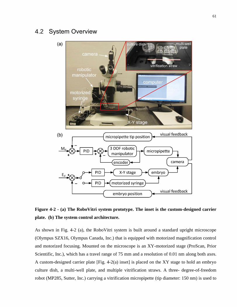
61
4.2 System Overview
Figure 4-2 - (a) The RoboVitri system prototype. The inset is the custom-designed carrier
plate. (b) The system control architecture.
As shown in Fig. 4-2 (a), the RoboVitri system is built around a standard upright microscope
(Olympus SZX16, Olympus Canada, Inc.) that is equipped with motorized magnification control
and motorized focusing. Mounted on the microscope is an XY-motorized stage (ProScan, Prior
Scientific, Inc.), which has a travel range of 75 mm and a resolution of 0.01 nm along both axes.
A custom-designed carrier plate [Fig. 4-2(a) inset] is placed on the XY stage to hold an embryo
culture dish, a multi-well plate, and multiple vitrification straws. A three- degree-of-freedom
robot (MP285, Sutter, Inc.) carrying a vitrification micropipette (tip diameter: 150 nm) is used to
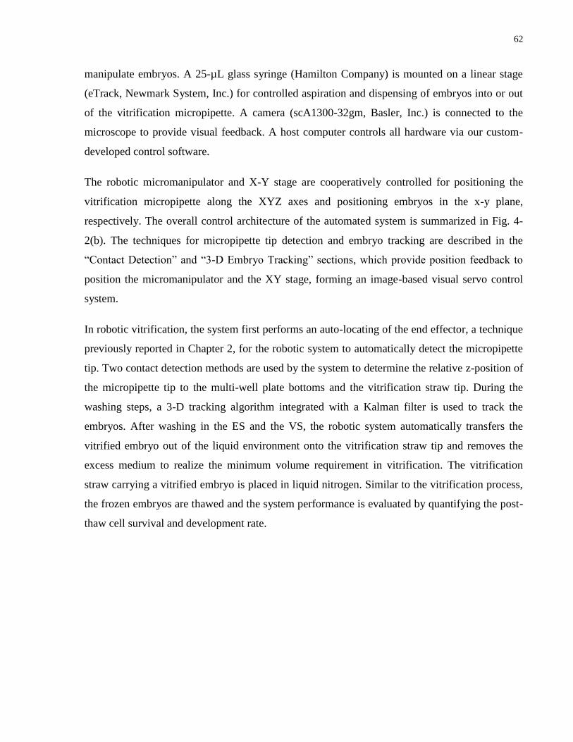
62
manipulate embryos. A 25-µL glass syringe (Hamilton Company) is mounted on a linear stage
(eTrack, Newmark System, Inc.) for controlled aspiration and dispensing of embryos into or out
of the vitrification micropipette. A camera (scA1300-32gm, Basler, Inc.) is connected to the
microscope to provide visual feedback. A host computer controls all hardware via our custom-
developed control software.
The robotic micromanipulator and X-Y stage are cooperatively controlled for positioning the
vitrification micropipette along the XYZ axes and positioning embryos in the x-y plane,
respectively. The overall control architecture of the automated system is summarized in Fig. 4-
2(b). The techniques for micropipette tip detection and embryo tracking are described in the
“Contact Detection” and “3-D Embryo Tracking” sections, which provide position feedback to
position the micromanipulator and the XY stage, forming an image-based visual servo control
system.
In robotic vitrification, the system first performs an auto-locating of the end effector, a technique
previously reported in Chapter 2, for the robotic system to automatically detect the micropipette
tip. Two contact detection methods are used by the system to determine the relative z-position of
the micropipette tip to the multi-well plate bottoms and the vitrification straw tip. During the
washing steps, a 3-D tracking algorithm integrated with a Kalman filter is used to track the
embryos. After washing in the ES and the VS, the robotic system automatically transfers the
vitrified embryo out of the liquid environment onto the vitrification straw tip and removes the
excess medium to realize the minimum volume requirement in vitrification. The vitrification
straw carrying a vitrified embryo is placed in liquid nitrogen. Similar to the vitrification process,
the frozen embryos are thawed and the system performance is evaluated by quantifying the post-
thaw cell survival and development rate.
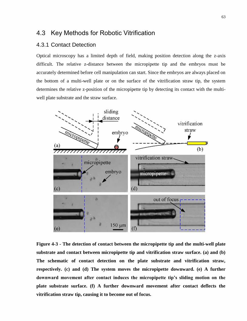
63
4.3 Key Methods for Robotic Vitrification
4.3.1 Contact Detection
Optical microscopy has a limited depth of field, making position detection along the z-axis
difficult. The relative z-distance between the micropipette tip and the embryos must be
accurately determined before cell manipulation can start. Since the embryos are always placed on
the bottom of a multi-well plate or on the surface of the vitrification straw tip, the system
determines the relative z-position of the micropipette tip by detecting its contact with the multi-
well plate substrate and the straw surface.
Figure 4-3 - The detection of contact between the micropipette tip and the multi-well plate
substrate and contact between micropipette tip and vitrification straw surface. (a) and (b)
The schematic of contact detection on the plate substrate and vitrification straw,
respectively. (c) and (d) The system moves the micropipette downward. (e) A further
downward movement after contact induces the micropipette tip’s sliding motion on the
plate substrate surface. (f) A further downward movement after contact deflects the
vitrification straw tip, causing it to become out of focus.
64
During contact detection on the multi-well plate substrate, the system moves the micropipette tip
downward to approach the plate substrate [Fig. 4-3(a) and (c)]. When the micropipette tip
contacts the plate bottom [Fig. 4-3(a) and (e)], further downward movement induces the tip‟s
horizontal sliding motion on the plate substrate, which changes the tip‟s position in the x-y plane
and the imaging plane. The system detects the initial x-y position change and, thus, determines
the initial contact of the vitrification micropipette tip with the plate substrate.
The detection of the micropipette tip contact on the vitrification straw surface is different from
contact detection with the multi-well plate bottom. Vitrification straw tips are cantilevers in
structure and have low stiffness compared with plate substrates. Therefore, instead of sliding on
the soft vitrification straw surface, the micropipette tip‟s further downward motion after initial
contact deflects the soft straw tip [Fig. 4-3(b)]. When the straw is deflected by the micropipette
tip, it becomes out of focus in imaging [Fig. 4-3(f)]. Based on the computed focus measure, the
robotic system detects the contact between the micropipette tip and the straw tip surface. This
contact detection step is critical before the robotic system can place the vitrified embryo onto the
straw tip, which will be discussed in the “Placing Embryo on Vitrification Straw” section.
4.3.2 Embryo Tracking in Three-Dimensional Space
The system, after detecting the micropipette tip positions along the XYZ axes relative to the
embryos, performs embryo pick and place to transfer the embryo from one type of solution to
another (e.g., from the ES to the VS) via controlled micropipette aspiration. Due to the changes
of fluid density and osmolarity, the embryo volume changes in the VS, resulting in variations of
buoyancy. In addition, the fluidic flow from the micropipette dispensing also influences the
embryo‟s positions. Thus, the embryos move dynamically in 3-D space when transferred into a
different VS. To avoid losing the embryo and to enable efficient pick and place for ensuring
stringent time control in each type of cryoprotectants, the robotic system must be able to robustly
detect and track embryos three-dimensionally.
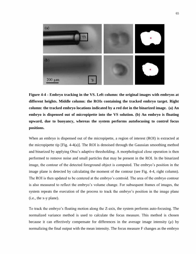
65
Figure 4-4 - Embryo tracking in the VS. Left column: the original images with embryos at
different heights. Middle column: the ROIs containing the tracked embryo target. Right
column: the tracked embryo locations indicated by a red dot in the binarized image. (a) An
embryo is dispensed out of micropipette into the VS solution. (b) An embryo is floating
upward, due to buoyancy, whereas the system performs autofocusing to control focus
positions.
When an embryo is dispensed out of the micropipette, a region of interest (ROI) is extracted at
the micropipette tip [Fig. 4-4(a)]. The ROI is denoised through the Gaussian smoothing method
and binarized by applying Otsu‟s adaptive thresholding. A morphological close operation is then
performed to remove noise and small particles that may be present in the ROI. In the binarized
image, the contour of the detected foreground object is computed. The embryo‟s position in the
image plane is detected by calculating the moment of the contour (see Fig. 4-4, right column).
The ROI is then updated to be centered at the embryo‟s centroid. The area of the embryo contour
is also measured to reflect the embryo‟s volume change. For subsequent frames of images, the
system repeats the execution of the process to track the embryo‟s position in the image plane
(i.e., the x-y plane).
To track the embryo‟s floating motion along the Z-axis, the system performs auto-focusing. The
normalized variance method is used to calculate the focus measure. This method is chosen
because it can effectively compensate for differences in the average image intensity (µ) by
normalizing the final output with the mean intensity. The focus measure F changes as the embryo
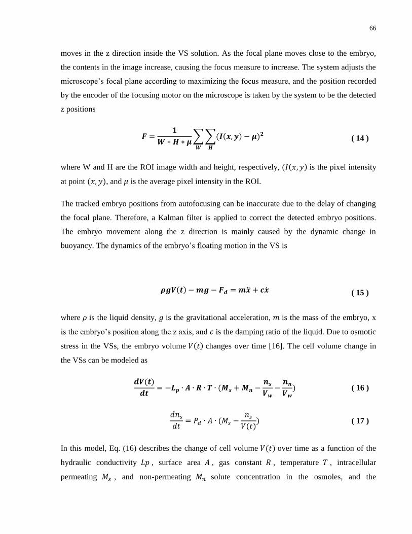
66
moves in the z direction inside the VS solution. As the focal plane moves close to the embryo,
the contents in the image increase, causing the focus measure to increase. The system adjusts the
microscope‟s focal plane according to maximizing the focus measure, and the position recorded
by the encoder of the focusing motor on the microscope is taken by the system to be the detected
z positions
∑∑
( 14 )
where W and H are the ROI image width and height, respectively, is the pixel intensity
at point , and is the average pixel intensity in the ROI.
The tracked embryo positions from autofocusing can be inaccurate due to the delay of changing
the focal plane. Therefore, a Kalman filter is applied to correct the detected embryo positions.
The embryo movement along the z direction is mainly caused by the dynamic change in
buoyancy. The dynamics of the embryo‟s floating motion in the VS is
( 15 )
where is the liquid density, is the gravitational acceleration, is the mass of the embryo, x
is the embryo‟s position along the z axis, and is the damping ratio of the liquid. Due to osmotic
stress in the VSs, the embryo volume changes over time [16]. The cell volume change in
the VSs can be modeled as
( 16 )
( 17 )
In this model, Eq. (16) describes the change of cell volume over time as a function of the
hydraulic conductivity , surface area , gas constant , temperature , intracellular
permeating , and non-permeating solute concentration in the osmoles, and the
67
extracellular permeating and non-permeating solute concentration. Equation (17) describes
the change in the intracellular moles of permeating solute ns over time as a function of the
DMSO permeability PD. When substituting into Eq. (17), the system analyzes the
dynamics of the embryo‟s 3-D motion and uses the Kalman filter to optimize the tracked results.
With the system dynamics modeled, the changes of embryo state in the VSs can be described by
choosing the XYZ positions and velocities as the state variables
( 18 )
where A is the state transition matrix, represents the noises affecting the actual state of the
embryo caused by the heterogeneous response of the individual embryos, and is assumed to
have a Gaussian distribution .
The embryo‟s position is calculated according to
( 19 )
where H is the output matrix and is the measurement noise, which is also assumed to have a
Gaussian distribution . is chosen based on the estimate of how accurately the
embryo‟s 3-D positions are detected by image processing.
Based on the dynamic model, a priori estimate of the state is computed
. The error covariance is denoted as . The priori estimate for this covariance at time is
then determined by
( 20 )
With the a priori estimate of the state and the measurement (i.e., the detected embryo
position from image processing), the real state of the embryo in the VS is optimized by
( 21 )
where is the Kalman gain and is given by
68
( 22 )
With the optimized embryo 3-D position , the robotic system controls the micropipette tip to
retrieve the embryo out of the solutions via controlled aspiration [184]. A biological advantage
of the embryo detection algorithm is that it enables the system to determine the optimized
processing time based on measuring the volume change of an embryo (i.e., individualized
timing, which is not possible to achieve in manual operation). In the VS, the embryos shrink in
the beginning due to osmotic pressure. Then they re-expand to equilibrate with the VS. Since the
cryoprotectant in the VS is toxic, the equilibration with the VS should be avoided [185].
Therefore, the robotic system retrieves and transfers the embryo out of the VS once its minimum
volume is reached, according to the 3-D tracking results.
4.3.3 Placing Embryo on Vitrification Straw
After washing the embryos in the ES and the VS under controlled timing, the vitrified embryos
need to be placed on a vitrification straw tip. In this step, the excess medium must be removed
from the vitrified embryo to ensure a high cooling rate in the liquid nitrogen. After detecting
contact of the micropipette tip and the straw surface, the system dispenses the embryo with a
relatively large volume of the VS solution onto the straw. The system then moves the
micropipette tip on the straw surface away from the initial dispensing location to form a thin VS
film [Fig. 4-5(a)]. The robotic system controls the motorized syringe to aspirate the VS until the
volume of the embryo droplet stops changing [Fig. 4-5(b)]. When the medium is aspirated into
the micropipette, a friction force acts on the embryo to keep it in the original place. To achieve
this, the fluid speed from micropipette aspiration must be well controlled.
As shown in Figure 4-5(c), the embryo is also acted on by the drag force generated by
micropipette aspiration flow
( 23 )
where is the fluid density, v is the fluid velocity controlled by the motorized syringe, is the
cross-sectional area, and is the drag coefficient. If the drag force is too large, the embryo can
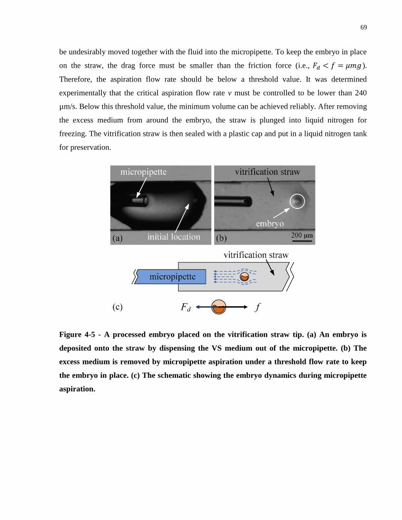
69
be undesirably moved together with the fluid into the micropipette. To keep the embryo in place
on the straw, the drag force must be smaller than the friction force (i.e., ).
Therefore, the aspiration flow rate should be below a threshold value. It was determined
experimentally that the critical aspiration flow rate v must be controlled to be lower than 240
µm/s. Below this threshold value, the minimum volume can be achieved reliably. After removing
the excess medium from around the embryo, the straw is plunged into liquid nitrogen for
freezing. The vitrification straw is then sealed with a plastic cap and put in a liquid nitrogen tank
for preservation.
Figure 4-5 - A processed embryo placed on the vitrification straw tip. (a) An embryo is
deposited onto the straw by dispensing the VS medium out of the micropipette. (b) The
excess medium is removed by micropipette aspiration under a threshold flow rate to keep
the embryo in place. (c) The schematic showing the embryo dynamics during micropipette
aspiration.
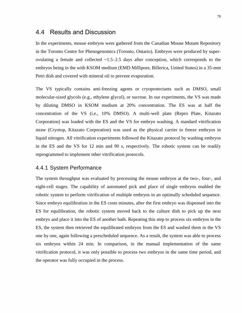
70
4.4 Results and Discussion
In the experiments, mouse embryos were gathered from the Canadian Mouse Mutant Repository
in the Toronto Centre for Phenogenomics (Toronto, Ontario). Embryos were produced by super-
ovulating a female and collected ~1.5–2.5 days after conception, which corresponds to the
embryos being in the with KSOM medium (EMD Millipore, Billerica, United States) in a 35-mm
Petri dish and covered with mineral oil to prevent evaporation.
The VS typically contains anti-freezing agents or cryoprotectants such as DMSO, small
molecular-sized glycols (e.g., ethylene glycol), or sucrose. In our experiments, the VS was made
by diluting DMSO in KSOM medium at 20% concentration. The ES was at half the
concentration of the VS (i.e., 10% DMSO). A multi-well plate (Repro Plate, Kitazato
Corporation) was loaded with the ES and the VS for embryo washing. A standard vitrification
straw (Cryotop, Kitazato Corporation) was used as the physical carrier to freeze embryos in
liquid nitrogen. All vitrification experiments followed the Kitazato protocol by washing embryos
in the ES and the VS for 12 min and 90 s, respectively. The robotic system can be readily
reprogrammed to implement other vitrification protocols.
4.4.1 System Performance
The system throughput was evaluated by processing the mouse embryos at the two-, four-, and
eight-cell stages. The capability of automated pick and place of single embryos enabled the
robotic system to perform vitrification of multiple embryos in an optimally scheduled sequence.
Since embryo equilibration in the ES costs minutes, after the first embryo was dispensed into the
ES for equilibration, the robotic system moved back to the culture dish to pick up the next
embryo and place it into the ES of another bath. Repeating this step to process six embryos in the
ES, the system then retrieved the equilibrated embryos from the ES and washed them in the VS
one by one, again following a prescheduled sequence. As a result, the system was able to process
six embryos within 24 min. In comparison, in the manual implementation of the same
vitrification protocol, it was only possible to process two embryos in the same time period, and
the operator was fully occupied in the process.
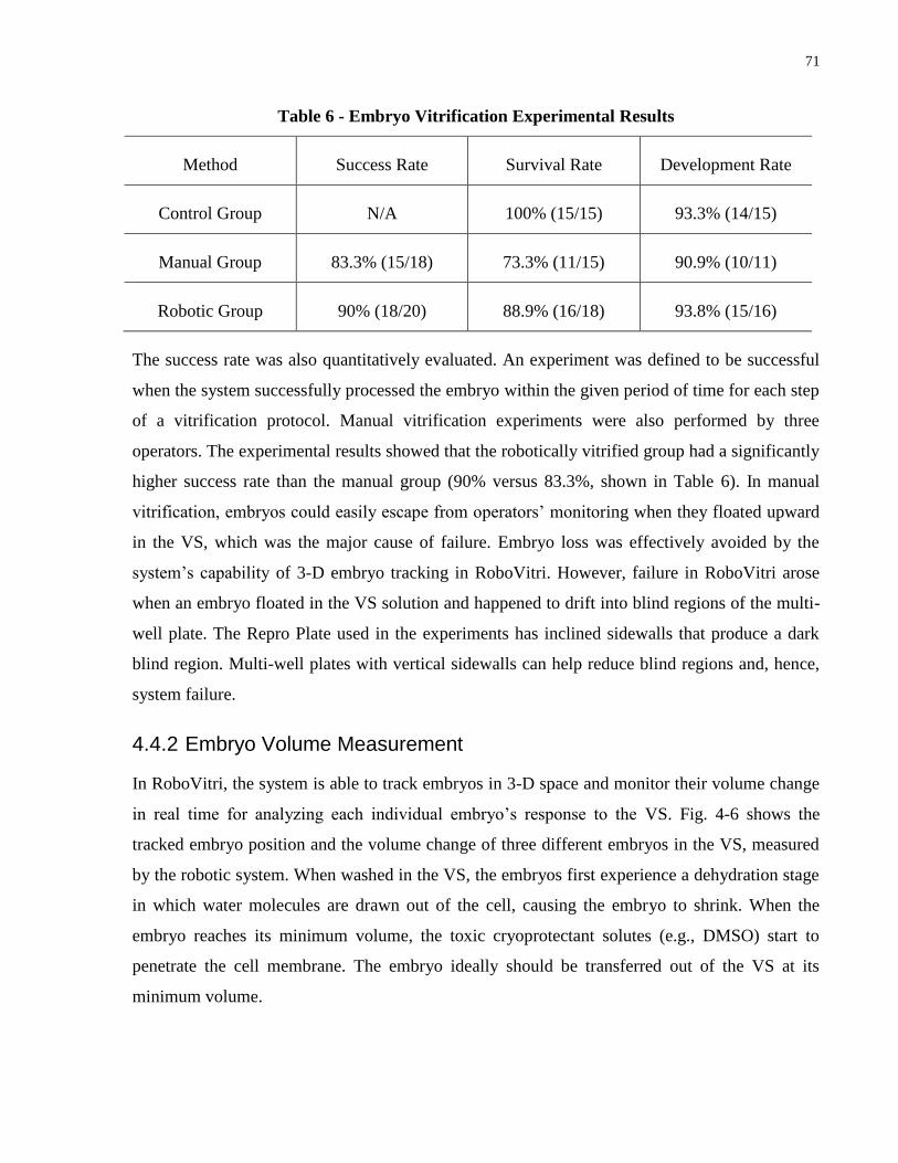
71
Table 6 - Embryo Vitrification Experimental Results
Method Success Rate Survival Rate Development Rate
Control Group N/A 100% (15/15) 93.3% (14/15)
Manual Group 83.3% (15/18) 73.3% (11/15) 90.9% (10/11)
Robotic Group 90% (18/20) 88.9% (16/18) 93.8% (15/16)
The success rate was also quantitatively evaluated. An experiment was defined to be successful
when the system successfully processed the embryo within the given period of time for each step
of a vitrification protocol. Manual vitrification experiments were also performed by three
operators. The experimental results showed that the robotically vitrified group had a significantly
higher success rate than the manual group (90% versus 83.3%, shown in Table 6). In manual
vitrification, embryos could easily escape from operators‟ monitoring when they floated upward
in the VS, which was the major cause of failure. Embryo loss was effectively avoided by the
system‟s capability of 3-D embryo tracking in RoboVitri. However, failure in RoboVitri arose
when an embryo floated in the VS solution and happened to drift into blind regions of the multi-
well plate. The Repro Plate used in the experiments has inclined sidewalls that produce a dark
blind region. Multi-well plates with vertical sidewalls can help reduce blind regions and, hence,
system failure.
4.4.2 Embryo Volume Measurement
In RoboVitri, the system is able to track embryos in 3-D space and monitor their volume change
in real time for analyzing each individual embryo‟s response to the VS. Fig. 4-6 shows the
tracked embryo position and the volume change of three different embryos in the VS, measured
by the robotic system. When washed in the VS, the embryos first experience a dehydration stage
in which water molecules are drawn out of the cell, causing the embryo to shrink. When the
embryo reaches its minimum volume, the toxic cryoprotectant solutes (e.g., DMSO) start to
penetrate the cell membrane. The embryo ideally should be transferred out of the VS at its
minimum volume.
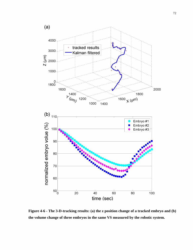
72
Figure 4-6 - The 3-D-tracking results: (a) the z position change of a tracked embryo and (b)
the volume change of three embryos in the same VS measured by the robotic system.
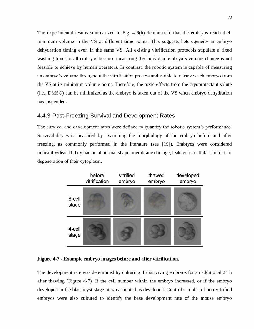
73
The experimental results summarized in Fig. 4-6(b) demonstrate that the embryos reach their
minimum volume in the VS at different time points. This suggests heterogeneity in embryo
dehydration timing even in the same VS. All existing vitrification protocols stipulate a fixed
washing time for all embryos because measuring the individual embryo‟s volume change is not
feasible to achieve by human operators. In contrast, the robotic system is capable of measuring
an embryo‟s volume throughout the vitrification process and is able to retrieve each embryo from
the VS at its minimum volume point. Therefore, the toxic effects from the cryoprotectant solute
(i.e., DMSO) can be minimized as the embryo is taken out of the VS when embryo dehydration
has just ended.
4.4.3 Post-Freezing Survival and Development Rates
The survival and development rates were defined to quantify the robotic system‟s performance.
Survivability was measured by examining the morphology of the embryo before and after
freezing, as commonly performed in the literature (see [19]). Embryos were considered
unhealthy/dead if they had an abnormal shape, membrane damage, leakage of cellular content, or
degeneration of their cytoplasm.
Figure 4-7 - Example embryo images before and after vitrification.
The development rate was determined by culturing the surviving embryos for an additional 24 h
after thawing (Figure 4-7). If the cell number within the embryo increased, or if the embryo
developed to the blastocyst stage, it was counted as developed. Control samples of non-vitrified
embryos were also cultured to identify the base development rate of the mouse embryo
74
population. Only embryos that had a healthy morphology after freezing were cultured following
similar procedures to other vitrification studies [20].
The experimental results are summarized in Table 6. The robotically vitrified group had higher
survival (88.9% versus 73.3%) and development rates (93.8% versus 90.9%) than the manually
vitrified group. The higher survival and development rates produced by RoboVitri can be
attributed to the optimized processing time achieved by the system through monitoring embryo
volume changes in the VS. The ability of the system to effectively remove excess medium from
around vitrified embryos on the straw (i.e., minimum volume vitrification for a higher cooling
rate when freezing in liquid nitrogen) could also have enabled the robotic system to achieve
higher embryo survival and development rates.
4.4.4 Discussion
Vitrification is an essential technique in IVF for preserving oocytes and embryos. A number of
different the VSs and protocols (e.g., Kitazato, Origio, and Irvine) have been developed and are
commercially available. All of these protocols require multiple steps of embryo washing in
different types of the VS. With the automated capability, our robotic system can be programmed
to test, optimize, and compare different vitrification protocols.
Besides embryo vitrification, oocyte vitrification is also important in IVF practice for preserving
female fertility for future use. Oocyte vitrification requires more steps than embryo vitrification.
For example, in the Kitazato protocol, oocyte vitrification involves three ES steps and two VS
steps, whereas embryo vitrification only has one ES and VS step. The RoboVitri system can also
be programmed to complete oocyte vitrification by simply repeating more washing steps because
of its capability of automated pick and place and stringent time control.
Robotic cell manipulation relieves the human operator from tedious vitrification steps and
eliminates manual operation-caused errors and inconsistencies. It also offers unparalleled timing
control and the ability to leave a minimal volume of the solution on vitrification straws.
Automation also enables the system to process multiple oocytes/embryos with high efficiency.
Efforts will continue to develop the system into an ideal tool for standardizing oocyte/embryo
vitrification in IVF clinics and to achieve improved cryopreservation outcomes.
75
4.5 Conclusion
This Chapter presented an automated RoboVitri system capable of processing embryos with
different the VS. The system is integrated with two contact detection methods to determine the
relative Z-position of the micropipette tip relative to embryos and vitrification straw tips. A 3-D
embryo-tracking technique was developed to prevent embryo loss during multiple washing steps
and achieve vision-guided embryo transfer. The 3-D embryo tracking technique also enables the
system to monitor real-time embryo volume changes in the VS, permitting individualized time
control for each embryo. In the step of placing an embryo onto the vitrification straw tip, the
excess medium was automatically aspirated away from the vitrified embryo to obtain a high
cooling rate. With these technical capabilities, the robotic system successfully achieved a high
throughput and improved post-freezing survival and development rates compared to manual
vitrification.
76
Chapter 5 Automated Analysis of Sperm Locomotion Behavior
Sperm selection plays a significant role in in vitro fertilization (IVF). Approaches for assessing
sperm quality include noninvasive techniques based on sperm morphology and motility as well
as invasive techniques for checking DNA integrity. In 2006, a new device using hyaluronic acid
(HA)-coated dish for sperm selection was cleared by the Food and Drug Administration (FDA)
and entered IVF clinics. In this technique, only sperms with DNA integrity bind to the HA
droplet, after which these bound sperms stop revealing head motion and their tail movement
becomes more vigorous. However, selecting a single sperm cell from among HA-bound sperms
is ad hoc in IVF clinics. Different from existing sperm tracking algorithms that are largely
limited to tracking sperm head only and are only able to track one sperm at a time, this chapter
presents a multi-sperm tracking algorithm that tracks both sperm heads and low-contrast sperm
tails. The tracking results confirm a significant correlation between sperm head velocity and tail
beating amplitude, demonstrate that sperms bound to HA generally have a higher velocity
(before binding) than those sperms that are not able to bind to HA microdots, and quantitatively
reveal that HA-bound sperms‟ tail beating amplitudes are different among HA-bound sperms.
The following section is based on the text from the following publication:
J. Liu, C. Leung, Z. Lu, and Y. Sun, "Quantitative analysis of locomotive behavior of human
sperm head and tail," IEEE Transactions on Biomedical Engineering, Vol. 60, pp. 390-396,
2013.
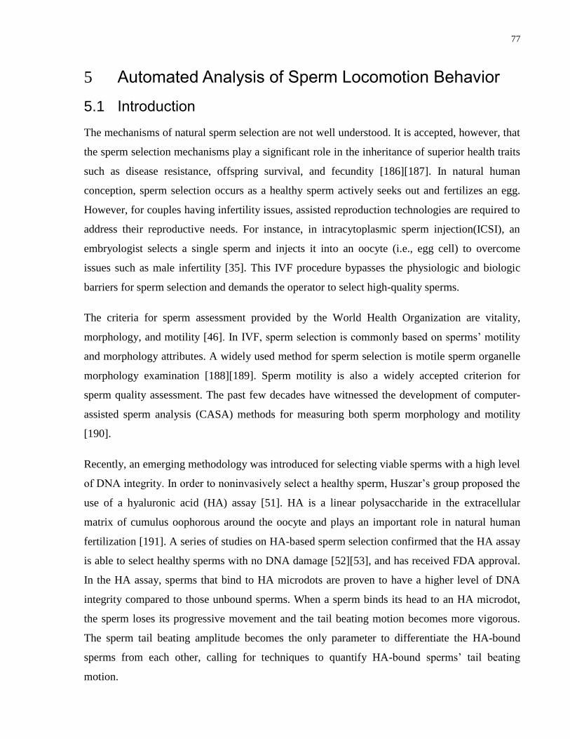
77
Automated Analysis of Sperm Locomotion Behavior 5
5.1 Introduction
The mechanisms of natural sperm selection are not well understood. It is accepted, however, that
the sperm selection mechanisms play a significant role in the inheritance of superior health traits
such as disease resistance, offspring survival, and fecundity [186][187]. In natural human
conception, sperm selection occurs as a healthy sperm actively seeks out and fertilizes an egg.
However, for couples having infertility issues, assisted reproduction technologies are required to
address their reproductive needs. For instance, in intracytoplasmic sperm injection(ICSI), an
embryologist selects a single sperm and injects it into an oocyte (i.e., egg cell) to overcome
issues such as male infertility [35]. This IVF procedure bypasses the physiologic and biologic
barriers for sperm selection and demands the operator to select high-quality sperms.
The criteria for sperm assessment provided by the World Health Organization are vitality,
morphology, and motility [46]. In IVF, sperm selection is commonly based on sperms‟ motility
and morphology attributes. A widely used method for sperm selection is motile sperm organelle
morphology examination [188][189]. Sperm motility is also a widely accepted criterion for
sperm quality assessment. The past few decades have witnessed the development of computer-
assisted sperm analysis (CASA) methods for measuring both sperm morphology and motility
[190].
Recently, an emerging methodology was introduced for selecting viable sperms with a high level
of DNA integrity. In order to noninvasively select a healthy sperm, Huszar‟s group proposed the
use of a hyaluronic acid (HA) assay [51]. HA is a linear polysaccharide in the extracellular
matrix of cumulus oophorous around the oocyte and plays an important role in natural human
fertilization [191]. A series of studies on HA-based sperm selection confirmed that the HA assay
is able to select healthy sperms with no DNA damage [52][53], and has received FDA approval.
In the HA assay, sperms that bind to HA microdots are proven to have a higher level of DNA
integrity compared to those unbound sperms. When a sperm binds its head to an HA microdot,
the sperm loses its progressive movement and the tail beating motion becomes more vigorous.
The sperm tail beating amplitude becomes the only parameter to differentiate the HA-bound
sperms from each other, calling for techniques to quantify HA-bound sperms‟ tail beating
motion.
78
Several algorithms have been reported for tracking multiple moving objects. Model-based
tracking algorithms incorporate priori information about the objects to develop representations
such as skin complexion [192], shape [193], kinematic skeleton [194], silhouettes [195], or layer
information [196]. Appearance-based approaches apply recognition algorithms to track objects in
eigenspace [197] derived from observations or in kernel space [198]. The correspondence of
multi-object tracking becomes complex with the presence of occlusions, misdetections, entries,
and exits of objects. Algorithms for solving the problems of nearby confuser and objects
occlusion/overlap include deterministic methods [199], single object state estimation (e.g.,
Kalman filter [200], particle filter [201]), and multiple object data association and state
estimation (e.g., global nearest neighbor method [202] and joint probability data association filter
[203]). Due to color uniformity and shape similarity of sperms, multi-sperm tracking has not
been well studied.
Several algorithms have been developed to track sperm trajectories, measure sperm velocities,
and evaluate sperm energetics [54], [204], [205]. Shi et al. reported a single-sperm tracking
algorithm based on a four-class thresholding method to extract a single sperm in a small region
of interest [55]. The method is limited to tracking a single sperm and is incapable of multi-sperm
tracking. Nafisi et al. demonstrated a template matching algorithm for sperm tracking. The
algorithm is insensitive to image acquisition conditions [56]. However, this algorithm relies on
user input to obtain the sperm‟s initial position and cannot track multiple sperms. Existing
algorithms for sperm tracking are largely limited to sperm head tracking. The small size (≤1 μm
in thickness) and low contrast of sperm tails under optical microscopy make sperm tail tracking
challenging. In our previous study [206], a maximum intensity region algorithm was developed
for sperm tail tracking. The tracking algorithm, without proper filtering, can be susceptible to
disturbances, such as overlapping of the target sperm with other sperms or debris and changes in
lighting conditions.
In this chapter, I report an approach for tracking both sperm head and tail. This approach uses a
motion template method to detect and track multiple moving sperms, and integrate a Kalman
filter to the maximum intensity region algorithm to locate the sperm tail‟s position. With the
positions of the sperm head and tail detected, the sperm‟s velocity and tail beating amplitude
were measured. Experimental results demonstrate that there is a significant correlation between
the sperm velocity and its tail beating amplitude. I also analyzed sperm motility and the tail
79
beating movement on HA coated dishes. I found that sperms with a higher level of motility are
more likely to bind to the HA microdots, and the sperm tail beating amplitude significantly
increases after a sperm binds to the HA microdots. Quantitative analysis of sperm tail‟s beating
amplitude can provide useful information for sperm selection.
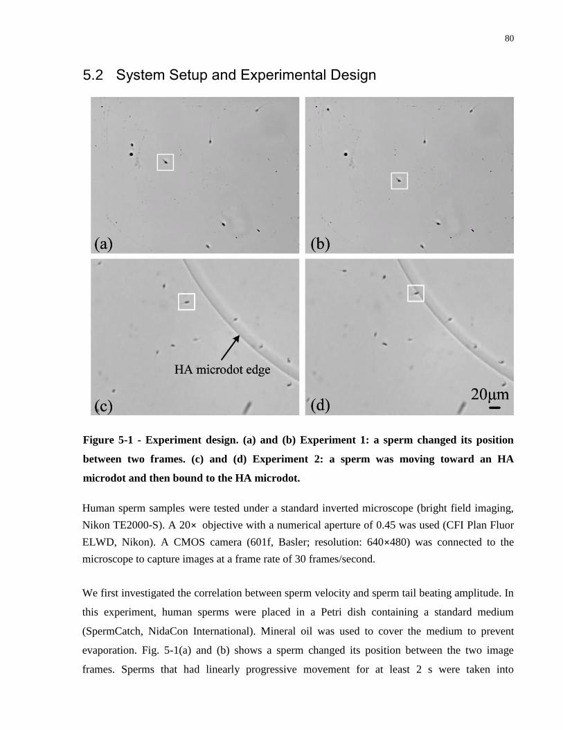
80
5.2 System Setup and Experimental Design
Figure 5-1 - Experiment design. (a) and (b) Experiment 1: a sperm changed its position
between two frames. (c) and (d) Experiment 2: a sperm was moving toward an HA
microdot and then bound to the HA microdot.
Human sperm samples were tested under a standard inverted microscope (bright field imaging,
Nikon TE2000-S). A 20× objective with a numerical aperture of 0.45 was used (CFI Plan Fluor
ELWD, Nikon). A CMOS camera (601f, Basler; resolution: 640×480) was connected to the
microscope to capture images at a frame rate of 30 frames/second.
We first investigated the correlation between sperm velocity and sperm tail beating amplitude. In
this experiment, human sperms were placed in a Petri dish containing a standard medium
(SpermCatch, NidaCon International). Mineral oil was used to cover the medium to prevent
evaporation. Fig. 5-1(a) and (b) shows a sperm changed its position between the two image
frames. Sperms that had linearly progressive movement for at least 2 s were taken into
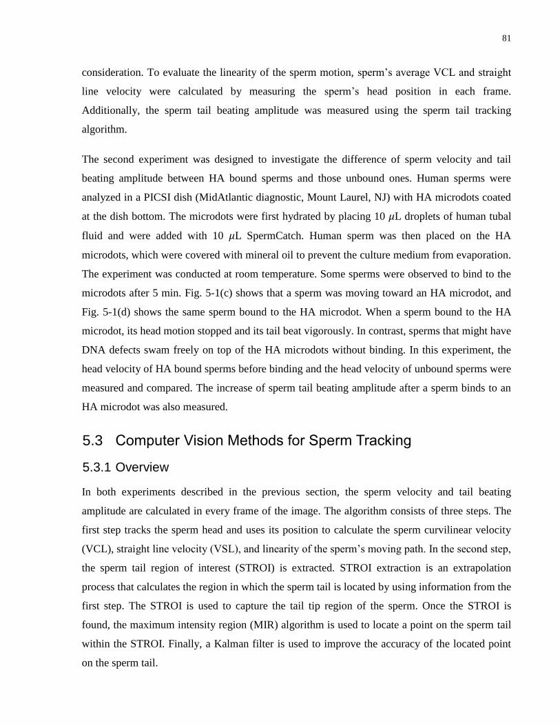
81
consideration. To evaluate the linearity of the sperm motion, sperm‟s average VCL and straight
line velocity were calculated by measuring the sperm‟s head position in each frame.
Additionally, the sperm tail beating amplitude was measured using the sperm tail tracking
algorithm.
The second experiment was designed to investigate the difference of sperm velocity and tail
beating amplitude between HA bound sperms and those unbound ones. Human sperms were
analyzed in a PICSI dish (MidAtlantic diagnostic, Mount Laurel, NJ) with HA microdots coated
at the dish bottom. The microdots were first hydrated by placing 10 μL droplets of human tubal
fluid and were added with 10 μL SpermCatch. Human sperm was then placed on the HA
microdots, which were covered with mineral oil to prevent the culture medium from evaporation.
The experiment was conducted at room temperature. Some sperms were observed to bind to the
microdots after 5 min. Fig. 5-1(c) shows that a sperm was moving toward an HA microdot, and
Fig. 5-1(d) shows the same sperm bound to the HA microdot. When a sperm bound to the HA
microdot, its head motion stopped and its tail beat vigorously. In contrast, sperms that might have
DNA defects swam freely on top of the HA microdots without binding. In this experiment, the
head velocity of HA bound sperms before binding and the head velocity of unbound sperms were
measured and compared. The increase of sperm tail beating amplitude after a sperm binds to an
HA microdot was also measured.
5.3 Computer Vision Methods for Sperm Tracking
5.3.1 Overview
In both experiments described in the previous section, the sperm velocity and tail beating
amplitude are calculated in every frame of the image. The algorithm consists of three steps. The
first step tracks the sperm head and uses its position to calculate the sperm curvilinear velocity
(VCL), straight line velocity (VSL), and linearity of the sperm‟s moving path. In the second step,
the sperm tail region of interest (STROI) is extracted. STROI extraction is an extrapolation
process that calculates the region in which the sperm tail is located by using information from the
first step. The STROI is used to capture the tail tip region of the sperm. Once the STROI is
found, the maximum intensity region (MIR) algorithm is used to locate a point on the sperm tail
within the STROI. Finally, a Kalman filter is used to improve the accuracy of the located point
on the sperm tail.
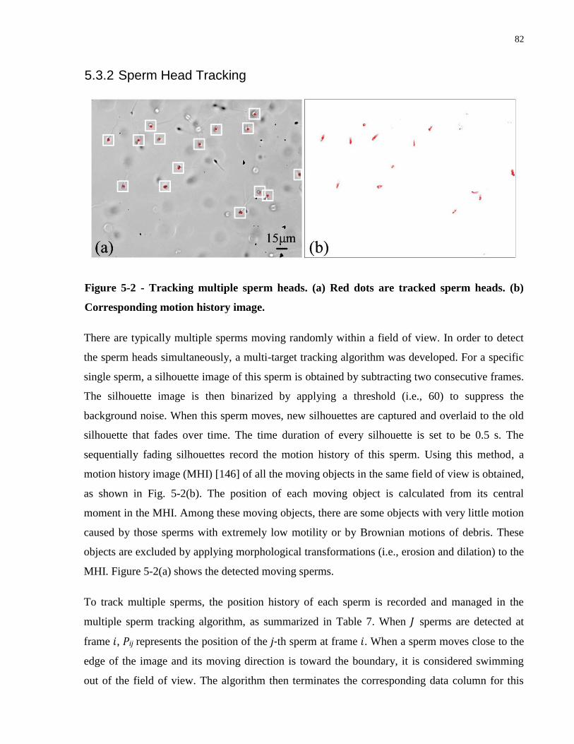
82
5.3.2 Sperm Head Tracking
Figure 5-2 - Tracking multiple sperm heads. (a) Red dots are tracked sperm heads. (b)
Corresponding motion history image.
There are typically multiple sperms moving randomly within a field of view. In order to detect
the sperm heads simultaneously, a multi-target tracking algorithm was developed. For a specific
single sperm, a silhouette image of this sperm is obtained by subtracting two consecutive frames.
The silhouette image is then binarized by applying a threshold (i.e., 60) to suppress the
background noise. When this sperm moves, new silhouettes are captured and overlaid to the old
silhouette that fades over time. The time duration of every silhouette is set to be 0.5 s. The
sequentially fading silhouettes record the motion history of this sperm. Using this method, a
motion history image (MHI) [146] of all the moving objects in the same field of view is obtained,
as shown in Fig. 5-2(b). The position of each moving object is calculated from its central
moment in the MHI. Among these moving objects, there are some objects with very little motion
caused by those sperms with extremely low motility or by Brownian motions of debris. These
objects are excluded by applying morphological transformations (i.e., erosion and dilation) to the
MHI. Figure 5-2(a) shows the detected moving sperms.
To track multiple sperms, the position history of each sperm is recorded and managed in the
multiple sperm tracking algorithm, as summarized in Table 7. When J sperms are detected at
frame , Pij represents the position of the j-th sperm at frame . When a sperm moves close to the
edge of the image and its moving direction is toward the boundary, it is considered swimming
out of the field of view. The algorithm then terminates the corresponding data column for this
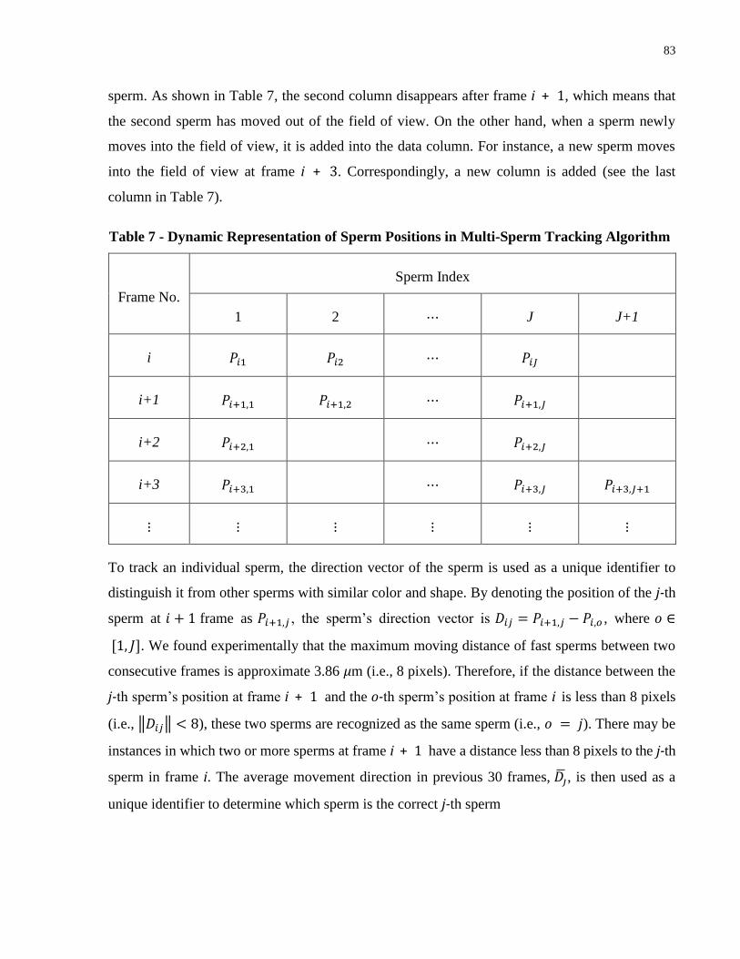
83
sperm. As shown in Table 7, the second column disappears after frame i + 1, which means that
the second sperm has moved out of the field of view. On the other hand, when a sperm newly
moves into the field of view, it is added into the data column. For instance, a new sperm moves
into the field of view at frame i + 3. Correspondingly, a new column is added (see the last
column in Table 7).
Table 7 - Dynamic Representation of Sperm Positions in Multi-Sperm Tracking Algorithm
Frame No.
Sperm Index
1 2 J J+1
i
i+1
i+2
i+3
To track an individual sperm, the direction vector of the sperm is used as a unique identifier to
distinguish it from other sperms with similar color and shape. By denoting the position of the j-th
sperm at frame as , the sperm‟s direction vector is , where ∈
. We found experimentally that the maximum moving distance of fast sperms between two
consecutive frames is approximate 3.86 μm (i.e., 8 pixels). Therefore, if the distance between the
j-th sperm‟s position at frame i + 1 and the o-th sperm‟s position at frame i is less than 8 pixels
(i.e., ‖ ‖ ), these two sperms are recognized as the same sperm (i.e., ). There may be
instances in which two or more sperms at frame i + 1 have a distance less than 8 pixels to the j-th
sperm in frame i. The average movement direction in previous 30 frames, , is then used as a
unique identifier to determine which sperm is the correct j-th sperm
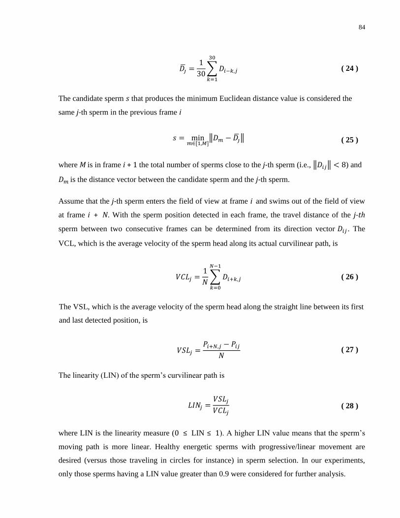
84
∑
( 24 )
The candidate sperm that produces the minimum Euclidean distance value is considered the
same j-th sperm in the previous frame i
∈
‖ ‖ ( 25 )
where M is in frame i + 1 the total number of sperms close to the j-th sperm (i.e., ‖ ‖ ) and
is the distance vector between the candidate sperm and the j-th sperm.
Assume that the j-th sperm enters the field of view at frame i and swims out of the field of view
at frame i + N. With the sperm position detected in each frame, the travel distance of the j-th
sperm between two consecutive frames can be determined from its direction vector . The
VCL, which is the average velocity of the sperm head along its actual curvilinear path, is
∑
( 26 )
The VSL, which is the average velocity of the sperm head along the straight line between its first
and last detected position, is
( 27 )
The linearity (LIN) of the sperm‟s curvilinear path is
( 28 )
where LIN is the linearity measure (0 ≤ LIN ≤ 1). A higher LIN value means that the sperm‟s
moving path is more linear. Healthy energetic sperms with progressive/linear movement are
desired (versus those traveling in circles for instance) in sperm selection. In our experiments,
only those sperms having a LIN value greater than 0.9 were considered for further analysis.
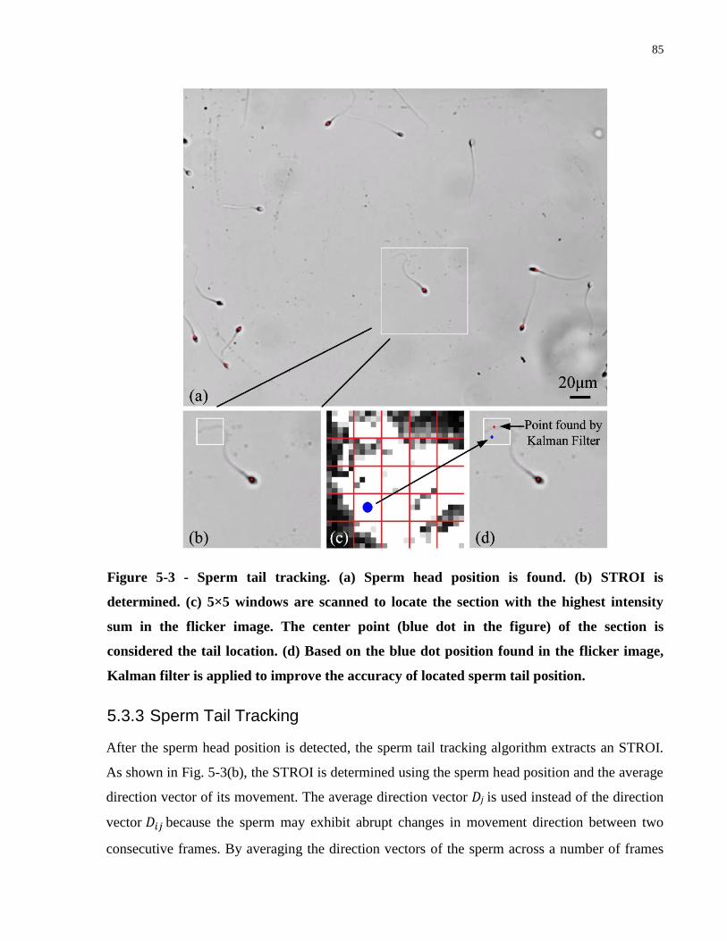
85
Figure 5-3 - Sperm tail tracking. (a) Sperm head position is found. (b) STROI is
determined. (c) 5×5 windows are scanned to locate the section with the highest intensity
sum in the flicker image. The center point (blue dot in the figure) of the section is
considered the tail location. (d) Based on the blue dot position found in the flicker image,
Kalman filter is applied to improve the accuracy of located sperm tail position.
5.3.3 Sperm Tail Tracking
After the sperm head position is detected, the sperm tail tracking algorithm extracts an STROI.
As shown in Fig. 5-3(b), the STROI is determined using the sperm head position and the average
direction vector of its movement. The average direction vector Dj is used instead of the direction
vector because the sperm may exhibit abrupt changes in movement direction between two
consecutive frames. By averaging the direction vectors of the sperm across a number of frames
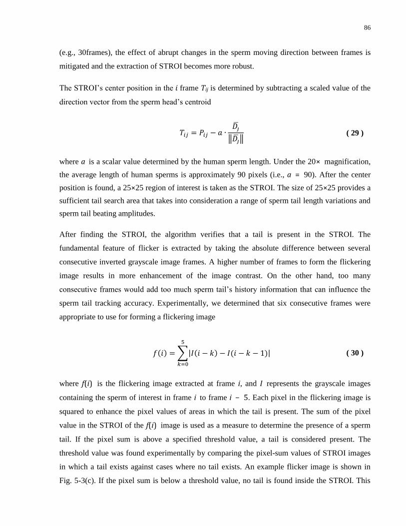
86
(e.g., 30frames), the effect of abrupt changes in the sperm moving direction between frames is
mitigated and the extraction of STROI becomes more robust.
The STROI‟s center position in the frame Tij is determined by subtracting a scaled value of the
direction vector from the sperm head‟s centroid
‖ ‖ ( 29 )
where a is a scalar value determined by the human sperm length. Under the 20× magnification,
the average length of human sperms is approximately 90 pixels (i.e., a = 90). After the center
position is found, a 25×25 region of interest is taken as the STROI. The size of 25×25 provides a
sufficient tail search area that takes into consideration a range of sperm tail length variations and
sperm tail beating amplitudes.
After finding the STROI, the algorithm verifies that a tail is present in the STROI. The
fundamental feature of flicker is extracted by taking the absolute difference between several
consecutive inverted grayscale image frames. A higher number of frames to form the flickering
image results in more enhancement of the image contrast. On the other hand, too many
consecutive frames would add too much sperm tail‟s history information that can influence the
sperm tail tracking accuracy. Experimentally, we determined that six consecutive frames were
appropriate to use for forming a flickering image
∑
( 30 )
where f(i) is the flickering image extracted at frame i, and I represents the grayscale images
containing the sperm of interest in frame i to frame i − 5. Each pixel in the flickering image is
squared to enhance the pixel values of areas in which the tail is present. The sum of the pixel
value in the STROI of the f(i) image is used as a measure to determine the presence of a sperm
tail. If the pixel sum is above a specified threshold value, a tail is considered present. The
threshold value was found experimentally by comparing the pixel-sum values of STROI images
in which a tail exists against cases where no tail exists. An example flicker image is shown in
Fig. 5-3(c). If the pixel sum is below a threshold value, no tail is found inside the STROI. This
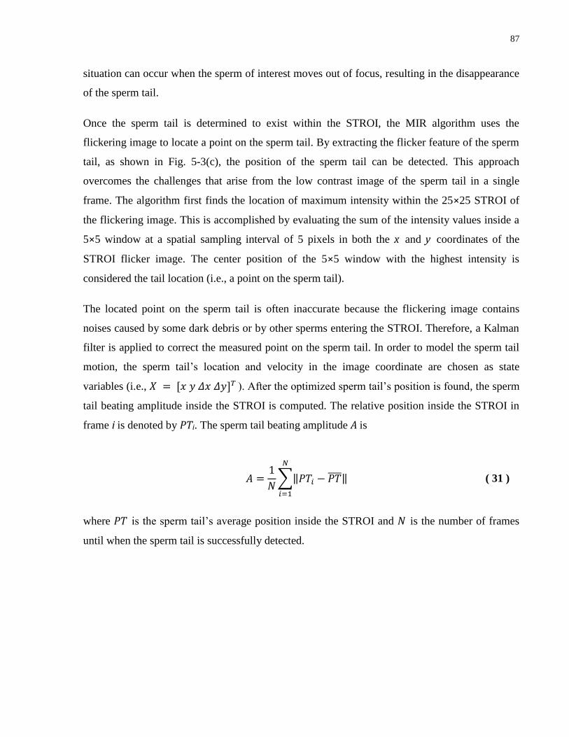
87
situation can occur when the sperm of interest moves out of focus, resulting in the disappearance
of the sperm tail.
Once the sperm tail is determined to exist within the STROI, the MIR algorithm uses the
flickering image to locate a point on the sperm tail. By extracting the flicker feature of the sperm
tail, as shown in Fig. 5-3(c), the position of the sperm tail can be detected. This approach
overcomes the challenges that arise from the low contrast image of the sperm tail in a single
frame. The algorithm first finds the location of maximum intensity within the 25×25 STROI of
the flickering image. This is accomplished by evaluating the sum of the intensity values inside a
5×5 window at a spatial sampling interval of 5 pixels in both the x and y coordinates of the
STROI flicker image. The center position of the 5×5 window with the highest intensity is
considered the tail location (i.e., a point on the sperm tail).
The located point on the sperm tail is often inaccurate because the flickering image contains
noises caused by some dark debris or by other sperms entering the STROI. Therefore, a Kalman
filter is applied to correct the measured point on the sperm tail. In order to model the sperm tail
motion, the sperm tail‟s location and velocity in the image coordinate are chosen as state
variables (i.e., ). After the optimized sperm tail‟s position is found, the sperm
tail beating amplitude inside the STROI is computed. The relative position inside the STROI in
frame i is denoted by PTi. The sperm tail beating amplitude A is
∑‖ ‖
( 31 )
where PT is the sperm tail‟s average position inside the STROI and N is the number of frames
until when the sperm tail is successfully detected.
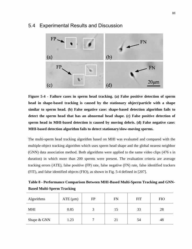
88
5.4 Experimental Results and Discussion
Figure 5-4 - Failure cases in sperm head tracking. (a) False positive detection of sperm
head in shape-based tracking is caused by the stationary object/particle with a shape
similar to sperm head. (b) False negative case: shape-based detection algorithm fails to
detect the sperm head that has an abnormal head shape. (c) False positive detection of
sperm head in MHI-based detection is caused by moving debris. (d) False negative case:
MHI-based detection algorithm fails to detect stationary/slow-moving sperms.
The multi-sperm head tracking algorithm based on MHI was evaluated and compared with the
multiple-object tracking algorithm which uses sperm head shape and the global nearest neighbor
(GNN) data association method. Both algorithms were applied to the same video clips (476 s in
duration) in which more than 200 sperms were present. The evaluation criteria are average
tracking errors (ATE), false positive (FP) rate, false negative (FN) rate, false identified trackers
(FIT), and false identified objects (FIO), as shown in Fig. 5-4 defined in [207].
Table 8 - Performance Comparison Between MHI-Based Multi-Sperm Tracking and GNN-
Based Multi-Sperm Tracking
Algorithms ATE (µm) FP FN FIT FIO
MHI 0.85 3 15 33 28
Shape & GNN 1.23 7 21 54 48
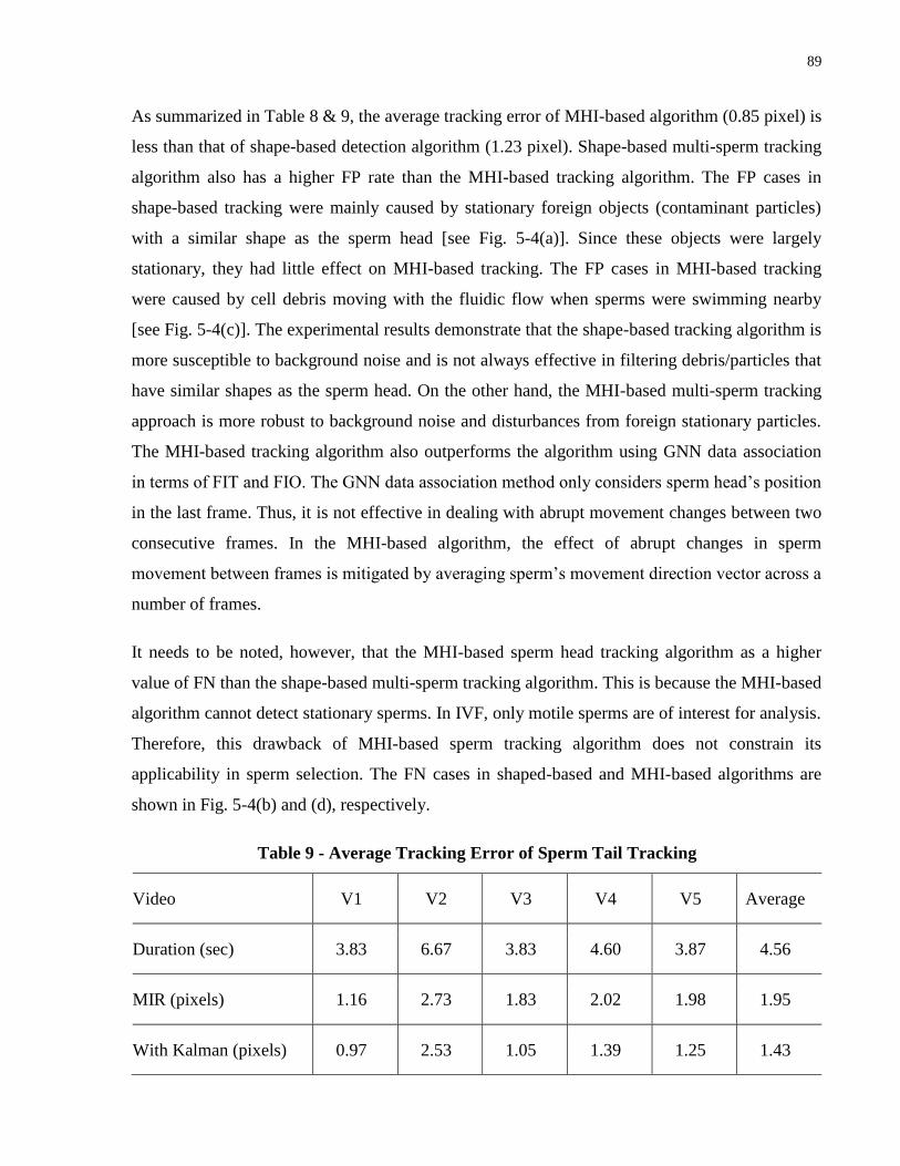
89
As summarized in Table 8 & 9, the average tracking error of MHI-based algorithm (0.85 pixel) is
less than that of shape-based detection algorithm (1.23 pixel). Shape-based multi-sperm tracking
algorithm also has a higher FP rate than the MHI-based tracking algorithm. The FP cases in
shape-based tracking were mainly caused by stationary foreign objects (contaminant particles)
with a similar shape as the sperm head [see Fig. 5-4(a)]. Since these objects were largely
stationary, they had little effect on MHI-based tracking. The FP cases in MHI-based tracking
were caused by cell debris moving with the fluidic flow when sperms were swimming nearby
[see Fig. 5-4(c)]. The experimental results demonstrate that the shape-based tracking algorithm is
more susceptible to background noise and is not always effective in filtering debris/particles that
have similar shapes as the sperm head. On the other hand, the MHI-based multi-sperm tracking
approach is more robust to background noise and disturbances from foreign stationary particles.
The MHI-based tracking algorithm also outperforms the algorithm using GNN data association
in terms of FIT and FIO. The GNN data association method only considers sperm head‟s position
in the last frame. Thus, it is not effective in dealing with abrupt movement changes between two
consecutive frames. In the MHI-based algorithm, the effect of abrupt changes in sperm
movement between frames is mitigated by averaging sperm‟s movement direction vector across a
number of frames.
It needs to be noted, however, that the MHI-based sperm head tracking algorithm as a higher
value of FN than the shape-based multi-sperm tracking algorithm. This is because the MHI-based
algorithm cannot detect stationary sperms. In IVF, only motile sperms are of interest for analysis.
Therefore, this drawback of MHI-based sperm tracking algorithm does not constrain its
applicability in sperm selection. The FN cases in shaped-based and MHI-based algorithms are
shown in Fig. 5-4(b) and (d), respectively.
Table 9 - Average Tracking Error of Sperm Tail Tracking
Video V1 V2 V3 V4 V5 Average
Duration (sec) 3.83 6.67 3.83 4.60 3.87 4.56
MIR (pixels) 1.16 2.73 1.83 2.02 1.98 1.95
With Kalman (pixels) 0.97 2.53 1.05 1.39 1.25 1.43
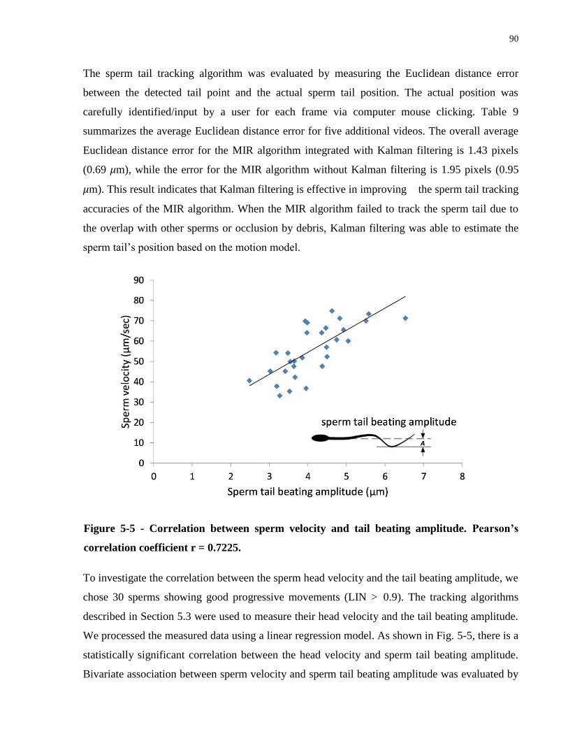
90
The sperm tail tracking algorithm was evaluated by measuring the Euclidean distance error
between the detected tail point and the actual sperm tail position. The actual position was
carefully identified/input by a user for each frame via computer mouse clicking. Table 9
summarizes the average Euclidean distance error for five additional videos. The overall average
Euclidean distance error for the MIR algorithm integrated with Kalman filtering is 1.43 pixels
(0.69 μm), while the error for the MIR algorithm without Kalman filtering is 1.95 pixels (0.95
μm). This result indicates that Kalman filtering is effective in improving the sperm tail tracking
accuracies of the MIR algorithm. When the MIR algorithm failed to track the sperm tail due to
the overlap with other sperms or occlusion by debris, Kalman filtering was able to estimate the
sperm tail‟s position based on the motion model.
Figure 5-5 - Correlation between sperm velocity and tail beating amplitude. Pearson’s
correlation coefficient r = 0.7225.
To investigate the correlation between the sperm head velocity and the tail beating amplitude, we
chose 30 sperms showing good progressive movements (LIN > 0.9). The tracking algorithms
described in Section 5.3 were used to measure their head velocity and the tail beating amplitude.
We processed the measured data using a linear regression model. As shown in Fig. 5-5, there is a
statistically significant correlation between the head velocity and sperm tail beating amplitude.
Bivariate association between sperm velocity and sperm tail beating amplitude was evaluated by
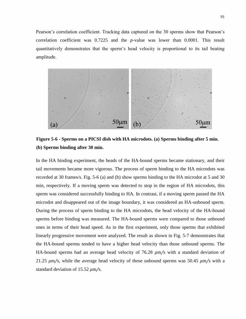
91
Pearson‟s correlation coefficient. Tracking data captured on the 30 sperms show that Pearson‟s
correlation coefficient was 0.7225 and the p-value was lower than 0.0001. This result
quantitatively demonstrates that the sperm‟s head velocity is proportional to its tail beating
amplitude.
Figure 5-6 - Sperms on a PICSI dish with HA microdots. (a) Sperms binding after 5 min.
(b) Sperms binding after 30 min.
In the HA binding experiment, the heads of the HA-bound sperms became stationary, and their
tail movements became more vigorous. The process of sperm binding to the HA microdots was
recorded at 30 frames/s. Fig. 5-6 (a) and (b) show sperms binding to the HA microdot at 5 and 30
min, respectively. If a moving sperm was detected to stop in the region of HA microdots, this
sperm was considered successfully binding to HA. In contrast, if a moving sperm passed the HA
microdot and disappeared out of the image boundary, it was considered an HA-unbound sperm.
During the process of sperm binding to the HA microdots, the head velocity of the HA-bound
sperms before binding was measured. The HA-bound sperms were compared to those unbound
ones in terms of their head speed. As in the first experiment, only those sperms that exhibited
linearly progressive movement were analyzed. The result as shown in Fig. 5-7 demonstrates that
the HA-bound sperms tended to have a higher head velocity than those unbound sperms. The
HA-bound sperms had an average head velocity of 76.28 μm/s with a standard deviation of
21.25 μm/s, while the average head velocity of those unbound sperms was 50.45 μm/s with a
standard deviation of 15.52 μm/s.
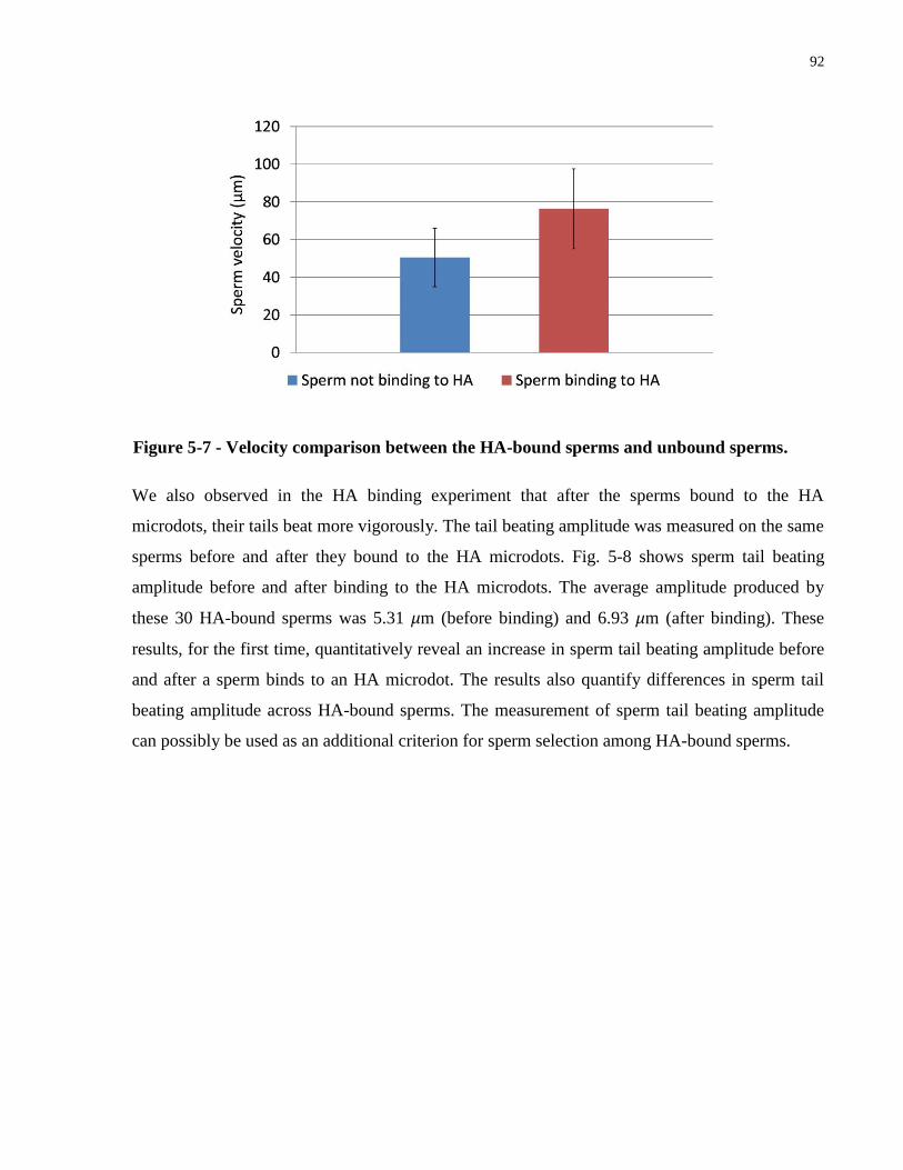
92
Figure 5-7 - Velocity comparison between the HA-bound sperms and unbound sperms.
We also observed in the HA binding experiment that after the sperms bound to the HA
microdots, their tails beat more vigorously. The tail beating amplitude was measured on the same
sperms before and after they bound to the HA microdots. Fig. 5-8 shows sperm tail beating
amplitude before and after binding to the HA microdots. The average amplitude produced by
these 30 HA-bound sperms was 5.31 μm (before binding) and 6.93 μm (after binding). These
results, for the first time, quantitatively reveal an increase in sperm tail beating amplitude before
and after a sperm binds to an HA microdot. The results also quantify differences in sperm tail
beating amplitude across HA-bound sperms. The measurement of sperm tail beating amplitude
can possibly be used as an additional criterion for sperm selection among HA-bound sperms.
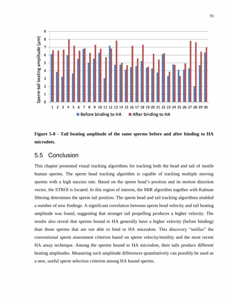
93
Figure 5-8 - Tail beating amplitude of the same sperms before and after binding to HA
microdots.
5.5 Conclusion
This chapter presented visual tracking algorithms for tracking both the head and tail of motile
human sperms. The sperm head tracking algorithm is capable of tracking multiple moving
sperms with a high success rate. Based on the sperm head‟s position and its motion direction
vector, the STROI is located. In this region of interest, the MIR algorithm together with Kalman
filtering determines the sperm tail position. The sperm head and tail tracking algorithms enabled
a number of new findings. A significant correlation between sperm head velocity and tail beating
amplitude was found, suggesting that stronger tail propelling produces a higher velocity. The
results also reveal that sperms bound to HA generally have a higher velocity (before binding)
than those sperms that are not able to bind to HA microdots. This discovery “unifies” the
conventional sperm assessment criterion based on sperm velocity/motility and the most recent
HA assay technique. Among the sperms bound to HA microdots, their tails produce different
beating amplitudes. Measuring such amplitude differences quantitatively can possibly be used as
a new, useful sperm selection criterion among HA bound sperms.
94
Chapter 6 Conclusions and Future Research
Conclusions and Future Research 6
This chapter summarizes the major contributions of this research and future research directions.
6.1 Contributions
In summary, this research focused on the development of new robotic systems and automated
methods for characterization and manipulation of single cells (e.g., cardiomyocyte, embryo and
sperm). This research has addressed two practical problems for robotic micromanipulations.
With the new technical solutions, two robotic prototype systems have been designed and built for
high throughput measurement of GJIC and automatically processing embryos for vitrification.
Additionally, quantitative analysis of sperm locomotion behaviors revealed interesting
correlations between sperm head movement speed and the tail beating motions. The combination
of sperm locomotion analysis with HA assay provides new solutions to assist doctors or
embryologists to select high-quality sperms for IVF applications.
The major contributions of this research are summarized as follows:
1. Developed the first automated method for locating end-effector tips. This method solved
the long-lasting practical problem of how to search for and locate end-effector tips for all
micromanipulation tasks. A summary of guidelines was provided for implementation of
this automated method.
2. Developed two modes of computer vision based contact detection algorithms for
determination of relative Z-positions of end-effector tips and single cells. Without the use
of extra sensors (e.g., force sensors or electrodes), these vision based methods were able
to determine the relative Z positions between end-effector tips and cells. The newly
developed methods were integrated into the first-of-its-kind robotic adherent cell
injection system and the robotic vitrification system.
3. Developed an automated system for robotic microinjection of adherent cells to measure
gap junctional intercellular communications. The powerful adherent cell injection system
95
was made possible by integrating several new techniques including automatically
locating micropipette tips, robustly detecting the contact of micropipette tip with the cell
membrane, and precisely compensating for accumulative positioning errors. The system
has been used to quantitatively measure GJIC for screening efficacy of selected drug
molecules.
4. Developed an automated system for robotic processing of mouse embryos for
vitrification. Robotic vitrification relieves the human operator from tedious vitrification
steps and eliminates manual operation-caused errors and inconsistencies. It also offers
unparalleled timing control based on monitoring embryo volume changes in real time.
5. Developed computer vision tracking algorithms for automated analysis of sperm head
and tail locomotion behavior. The analysis of both sperm head and tail locomotion
behaviors revealed a significant correlation between sperm head velocity and tail beating
amplitude, suggesting that stronger tail propelling produces a higher velocity. The results
also showed that sperms bound to HA generally have a higher velocity (before binding)
than those sperms that are not able to bind to HA microdots. These results provided new
information to assist the selection of high-quality of human sperm in IVF clinics.
6.2 Future Research
6.2.1 Improvement of the Present Research
Despite the significant progress of the present research, there are still many opportunities
remaining for further improvement of the robotic systems and automated techniques for
characterization and manipulation of single cells. Several exemplary future research topics are:
Fully automated robotic injection system is required to screen a high number of FDA-
approved drug molecules. In order to achieve a fully automated system, a robust single
cell detection method needs to be developed to recognize the optimal injection locations
on individual cells for injection.
Gap junctions facilitate both diffusion of small molecules and conduction of ions between
adjacent cells. Gap junction conductance measurement can be performed by using a
double whole-cell patch clamp system or optical mapping technique. Future research
96
should involve the development of robotic automation approaches to achieve high
throughput measurement of electrical conduction.
To further increase the throughput of the robotic vitrification system, new functions such
as controlled aspiration of multiple embryos at one time are needed. Along this direction,
future research should focus on microfluidic modeling and controller design to accurately
position multiple embryos with equal distance inside a micropipette.
In the present robotic vitrification system, the last step still needs a technician to
manually pick up and plunge vitrification straws with vitrified embryos into liquid
nitrogen for cryopreservation. To fully eliminate human involvement in the vitrification
procedure, future research can focus on the development of a robotic pick-and-place
manipulator (e.g., a 3-DOF robotic arm with a gripper) to automatically freeze
vitrification straws in liquid nitrogen.
At present, the newly-developed robotic vitrification system was tested by using mouse
embryos. Future work should include more testing on mouse oocytes for oocyte
vitrification.
The current robotic vitrification system is designed to retrieve the embryos out of VS at
their minimum volume to reduce the toxic effects of DMSO. Future testing should
include the performance comparison between the individualized time control in the
robotic system and a fixed VS washing protocol to experimentally validate the theory of
minimizing toxic effects by real-time monitoring oocytes/embryo volume change.
The automated sperm analysis method in this research is able to extract the sperm tail
beating amplitude and use it to investigate the sperm locomotion behaviors. However, the
sperm forward movement also depends on the sperm beating frequency. Further
investigation should be conducted to measure the sperm tail-beating frequency by
developing new computer vision algorithms with high-speed imaging techniques (e.g.,
over 100 fps).
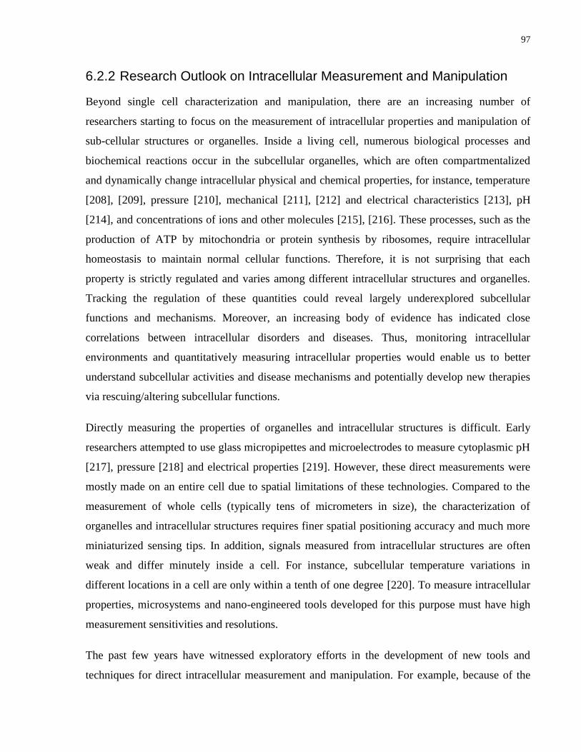
97
6.2.2 Research Outlook on Intracellular Measurement and Manipulation
Beyond single cell characterization and manipulation, there are an increasing number of
researchers starting to focus on the measurement of intracellular properties and manipulation of
sub-cellular structures or organelles. Inside a living cell, numerous biological processes and
biochemical reactions occur in the subcellular organelles, which are often compartmentalized
and dynamically change intracellular physical and chemical properties, for instance, temperature
[208], [209], pressure [210], mechanical [211], [212] and electrical characteristics [213], pH
[214], and concentrations of ions and other molecules [215], [216]. These processes, such as the
production of ATP by mitochondria or protein synthesis by ribosomes, require intracellular
homeostasis to maintain normal cellular functions. Therefore, it is not surprising that each
property is strictly regulated and varies among different intracellular structures and organelles.
Tracking the regulation of these quantities could reveal largely underexplored subcellular
functions and mechanisms. Moreover, an increasing body of evidence has indicated close
correlations between intracellular disorders and diseases. Thus, monitoring intracellular
environments and quantitatively measuring intracellular properties would enable us to better
understand subcellular activities and disease mechanisms and potentially develop new therapies
via rescuing/altering subcellular functions.
Directly measuring the properties of organelles and intracellular structures is difficult. Early
researchers attempted to use glass micropipettes and microelectrodes to measure cytoplasmic pH
[217], pressure [218] and electrical properties [219]. However, these direct measurements were
mostly made on an entire cell due to spatial limitations of these technologies. Compared to the
measurement of whole cells (typically tens of micrometers in size), the characterization of
organelles and intracellular structures requires finer spatial positioning accuracy and much more
miniaturized sensing tips. In addition, signals measured from intracellular structures are often
weak and differ minutely inside a cell. For instance, subcellular temperature variations in
different locations in a cell are only within a tenth of one degree [220]. To measure intracellular
properties, microsystems and nano-engineered tools developed for this purpose must have high
measurement sensitivities and resolutions.
The past few years have witnessed exploratory efforts in the development of new tools and
techniques for direct intracellular measurement and manipulation. For example, because of the
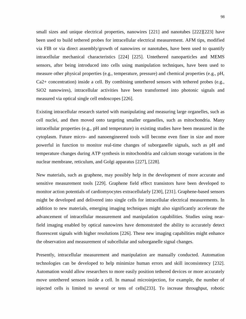
98
small sizes and unique electrical properties, nanowires [221] and nanotubes [222][223] have
been used to build tethered probes for intracellular electrical measurement. AFM tips, modified
via FIB or via direct assembly/growth of nanowires or nanotubes, have been used to quantify
intracellular mechanical characteristics [224] [225]. Untethered nanoparticles and MEMS
sensors, after being introduced into cells using manipulation techniques, have been used to
measure other physical properties (e.g., temperature, pressure) and chemical properties (e.g., pH,
Ca2+ concentration) inside a cell. By combining untethered sensors with tethered probes (e.g.,
SiO2 nanowires), intracellular activities have been transformed into photonic signals and
measured via optical single cell endoscopes [226].
Existing intracellular research started with manipulating and measuring large organelles, such as
cell nuclei, and then moved onto targeting smaller organelles, such as mitochondria. Many
intracellular properties (e.g., pH and temperature) in existing studies have been measured in the
cytoplasm. Future micro- and nanoengineered tools will become even finer in size and more
powerful in function to monitor real-time changes of suborganelle signals, such as pH and
temperature changes during ATP synthesis in mitochondria and calcium storage variations in the
nuclear membrane, reticulum, and Golgi apparatus [227], [228].
New materials, such as graphene, may possibly help in the development of more accurate and
sensitive measurement tools [229]. Graphene field effect transistors have been developed to
monitor action potentials of cardiomyocytes extracellularly [230], [231]. Graphene-based sensors
might be developed and delivered into single cells for intracellular electrical measurements. In
addition to new materials, emerging imaging techniques might also significantly accelerate the
advancement of intracellular measurement and manipulation capabilities. Studies using near-
field imaging enabled by optical nanowires have demonstrated the ability to accurately detect
fluorescent signals with higher resolutions [226]. These new imaging capabilities might enhance
the observation and measurement of subcellular and suborganelle signal changes.
Presently, intracellular measurement and manipulation are manually conducted. Automation
technologies can be developed to help minimize human errors and skill inconsistency [232].
Automation would allow researchers to more easily position tethered devices or more accurately
move untethered sensors inside a cell. In manual microinjection, for example, the number of
injected cells is limited to several or tens of cells[233]. To increase throughput, robotic
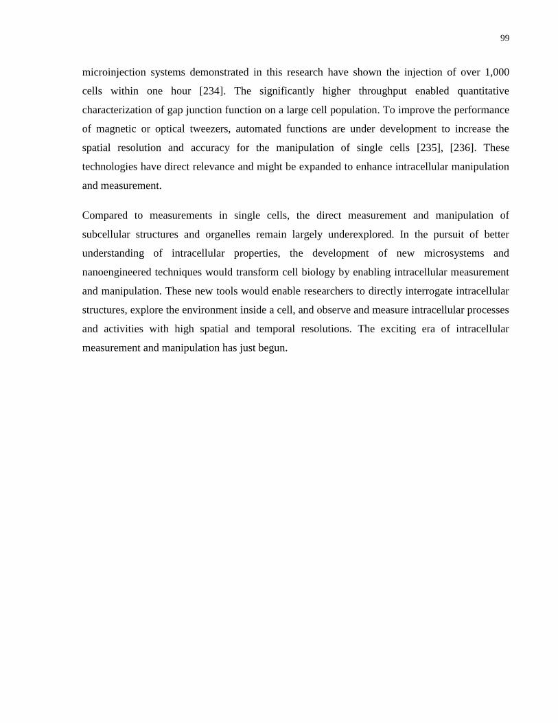
99
microinjection systems demonstrated in this research have shown the injection of over 1,000
cells within one hour [234]. The significantly higher throughput enabled quantitative
characterization of gap junction function on a large cell population. To improve the performance
of magnetic or optical tweezers, automated functions are under development to increase the
spatial resolution and accuracy for the manipulation of single cells [235], [236]. These
technologies have direct relevance and might be expanded to enhance intracellular manipulation
and measurement.
Compared to measurements in single cells, the direct measurement and manipulation of
subcellular structures and organelles remain largely underexplored. In the pursuit of better
understanding of intracellular properties, the development of new microsystems and
nanoengineered techniques would transform cell biology by enabling intracellular measurement
and manipulation. These new tools would enable researchers to directly interrogate intracellular
structures, explore the environment inside a cell, and observe and measure intracellular processes
and activities with high spatial and temporal resolutions. The exciting era of intracellular
measurement and manipulation has just begun.

100
References
[1] J. E. Ferrell and E. M. Machleder, “The Biochemical Basis of an All-or-None Cell Fate
Switch in Xenopus Oocytes,” Sci. , vol. 280 , no. 5365 , pp. 895–898, May 1998.
[2] J.-H. Chen, C. Y. Y. Yip, E. D. Sone, and C. A. Simmons, “Identification and
Characterization of Aortic Valve Mesenchymal Progenitor Cells with Robust Osteogenic
Calcification Potential,” Am. J. Pathol., vol. 174, no. 3, pp. 1109–1119, Mar. 2009.
[3] S. D. Carson and S. J. Pirruccello, “HeLa cell heterogeneity and coxsackievirus B3
cytopathic effect: Implications for inter-laboratory reproducibility of results,” J. Med.
Virol., vol. 85, no. 4, pp. 677–683, Apr. 2013.
[4] X. Wang, “Heterogeneity in the HeLa Cell Cycle Response to UVC Analyzed by the
BrdUrd Two-Parameter Method,” Exp. Cell Res., vol. 212, no. 2, pp. 176–189, Jun. 1994.
[5] M. B. Elowitz, “Stochastic Gene Expression in a Single Cell,” Science (80-. )., vol. 297,
no. 5584, pp. 1183–1186, Aug. 2002.
[6] P. D. Bhola and S. M. Simon, “Determinism and divergence of apoptosis susceptibility in
mammalian cells.,” J. Cell Sci., vol. 122, no. Pt 23, pp. 4296–302, Dec. 2009.
[7] X. Xia, M. S. Owen, R. E. C. Lee, and S. Gaudet, “Cell-to-cell variability in cell death :
can systems biology help us make sense of it all ?” vol. 5, no. 5, pp. e1261–11, 2014.
[8] J. Liu, C. Moraes, Z. Lu, C. Simmons, and Y. Sun, “Single Cell Deposition,” 2012, pp.
403–420.
[9] C. Gawad, W. Koh, and S. R. Quake, “Single-cell genome sequencing: current state of the
science,” Nat. Rev. Genet., vol. 17, no. 3, pp. 175–188, Jan. 2016.
[10] O. Schwartzman and A. Tanay, “Single-cell epigenomics: techniques and emerging
applications,” Nat. Rev. Genet., vol. 16, no. 12, pp. 716–726, Oct. 2015.
[11] P. Liberali, B. Snijder, and L. Pelkmans, “Single-cell and multivariate approaches in
genetic perturbation screens,” Nat. Rev. Genet., vol. 16, no. 1, pp. 18–32, Dec. 2014.
101
[12] J. Czyz, U. Irmer, G. Schulz, A. Mindermann, and D. F. Hülser, “Gap-junctional coupling
measured by flow cytometry.,” Exp. Cell Res., vol. 255, no. 1, pp. 40–6, Feb. 2000.
[13] E. L. Hertzberg, T. S. Lawrence, and N. B. Gilula, “Gap Junctional Communication,”
Annu. Rev. Physiol., vol. 43, no. 1, pp. 479–491, Oct. 1981.
[14] N. S. Heyman, D. T. Kurjiaka, J. F. Ek Vitorin, and J. M. Burt, “Regulation of gap
junctional charge selectivity in cells coexpressing connexin 40 and connexin 43,” AJP
Hear. Circ. Physiol., vol. 297, no. 1, pp. H450–H459, Jul. 2009.
[15] P. R. Brink, K. Cronin, and S. V. Ramanan, “Gap junctions in excitable cells,” J.
Bioenerg. Biomembr., vol. 28, no. 4, pp. 351–358, Aug. 1996.
[16] G. H. Kalimi and C. W. Lo, “Gap junctional communication in the extraembryonic tissues
of the gastrulating mouse embryo.,” J. Cell Biol., vol. 109, no. 6 Pt 1, pp. 3015–26, Dec.
1989.
[17] W. R. Loewenstein, “Junctional intercellular communication: the cell-to-cell membrane
channel.,” Physiol. Rev., vol. 61, no. 4, pp. 829–913, Oct. 1981.
[18] M. M. Vance and L. M. Wiley, “Gap junction intercellular communication mediates the
competitive cell proliferation disadvantage of irradiated mouse preimplantation embryos
in aggregation chimeras.,” Radiat. Res., vol. 152, no. 5, pp. 544–51, Nov. 1999.
[19] D. E. Gutstein, “Focal gap junction uncoupling and spontaneous ventricular ectopy,” AJP
Hear. Circ. Physiol., vol. 289, no. 3, pp. H1091–H1098, May 2005.
[20] M. Strom, X. Wan, S. Poelzing, E. Ficker, and D. S. Rosenbaum, “Gap junction
heterogeneity as mechanism for electrophysiologically distinct properties across the
ventricular wall.,” Am. J. Physiol. Heart Circ. Physiol., vol. 298, no. 3, pp. H787–94, Mar.
2010.
[21] S. S. Chugh, K. Reinier, C. Teodorescu, A. Evanado, E. Kehr, M. Al Samara, R. Mariani,
K. Gunson, and J. Jui, “Epidemiology of sudden cardiac death: clinical and research
implications.,” Prog. Cardiovasc. Dis., vol. 51, no. 3, pp. 213–28.
102
[22] J. F. Ek-Vitorin and J. M. Burt, “Structural basis for the selective permeability of channels
made of communicating junction proteins.,” Biochim. Biophys. Acta, vol. 1828, no. 1, pp.
51–68, Jan. 2013.
[23] M. Rackauskas, V. Neverauskas, and V. A. Skeberdis, “Diversity and properties of
connexin gap junction channels.,” Medicina (Kaunas)., vol. 46, no. 1, pp. 1–12, 2010.
[24] D. B. Alexander and G. S. Goldberg, “Transfer of biologically important molecules
between cells through gap junction channels.,” Curr. Med. Chem., vol. 10, no. 19, pp.
2045–58, Oct. 2003.
[25] L. H. Raptis, H. L. Brownell, K. L. Firth, and L. W. Mackenzie, “A novel technique for
the study of intercellular, junctional communication: electroporation of adherent cells on a
partly conductive slide.,” DNA Cell Biol., vol. 13, no. 9, pp. 963–75, Sep. 1994.
[26] J.-C. Hervé, N. Bourmeyster, and D. Sarrouilhe, “Diversity in protein-protein interactions
of connexins: emerging roles.,” Biochim. Biophys. Acta, vol. 1662, no. 1–2, pp. 22–41,
Mar. 2004.
[27] D. J. Fitzgerald and A. W. Murray, “Inhibition of intercellular communication by tumor-
promoting phorbol esters.,” Cancer Res., vol. 40, no. 8 Pt 1, pp. 2935–7, Aug. 1980.
[28] M. H. El-Fouly, J. E. Trosko, and C.-C. Chang, “Scrape-loading and dye transfer,” Exp.
Cell Res., vol. 168, no. 2, pp. 422–430, Feb. 1987.
[29] L. H. Raptis, H. L. Brownell, K. L. Firth, and L. W. Mackenzie, “A novel technique for
the study of intercellular, junctional communication: electroporation of adherent cells on a
partly conductive slide.,” DNA Cell Biol., vol. 13, no. 9, pp. 963–75, Sep. 1994.
[30] M. H. Wade, J. E. Trosko, and M. Schindler, “A fluorescence photobleaching assay of gap
junction-mediated communication between human cells.,” Science, vol. 232, no. 4749, pp.
525–8, Apr. 1986.
[31] M. L. McCain, T. Desplantez, N. A. Geisse, B. Rothen-Rutishauser, H. Oberer, K. K.
Parker, and A. G. Kleber, “Cell-to-cell coupling in engineered pairs of rat ventricular
cardiomyocytes: relation between Cx43 immunofluorescence and intercellular electrical
103
conductance.,” Am. J. Physiol. Heart Circ. Physiol., vol. 302, no. 2, pp. H443–50, Jan.
2012.
[32] M. Abbaci, M. Barberi-Heyob, W. Blondel, F. Guillemin, and J. Didelon, “Advantages
and limitations of commonly used methods to assay the molecular permeability of gap
junctional intercellular communication.,” Biotechniques, vol. 45, no. 1, pp. 33–52, 56–62,
Jul. 2008.
[33] M. H. Juul, E. Rivedal, T. Stokke, and T. Sanner, “Quantitative determination of gap
junction intercellular communication using flow cytometric measurement of fluorescent
dye transfer.,” Cell Adhes. Commun., vol. 7, no. 6, pp. 501–12, 2000.
[34] J. Boivin, L. Bunting, J. A. Collins, and K. G. Nygren, “International estimates of
infertility prevalence and treatment-seeking: potential need and demand for infertility
medical care,” Hum. Reprod., vol. 22, no. 6, pp. 1506–1512, Mar. 2007.
[35] G. Palermo, H. Joris, P. Devroey, and A. C. Van Steirteghem, “Pregnancies after
intracytoplasmic injection of single spermatozoon into an oocyte.,” Lancet (London,
England), vol. 340, no. 8810, pp. 17–8, Jul. 1992.
[36] P. Devroey, “A review of ten years experience of ICSI,” Hum. Reprod. Update, vol. 10,
no. 1, pp. 19–28, Jan. 2004.
[37] J. Konc, K. Kanyó, R. Kriston, B. Somoskői, and S. Cseh, “Cryopreservation of Embryos
and Oocytes in Human Assisted Reproduction,” Biomed Res. Int., vol. 2014, pp. 1–9,
2014.
[38] J. Boldt, “Human oocyte cryopreservation as an adjunct to IVF-embryo transfer cycles,”
Hum. Reprod., vol. 18, no. 6, pp. 1250–1255, Jun. 2003.
[39] M. Kuwayama, G. Vajta, O. Kato, and S. P. Leibo, “Highly efficient vitrification method
for cryopreservation of human oocytes,” Reprod. Biomed. Online, vol. 11, no. 3, pp. 300–
308, Jan. 2005.
[40] R. Riggs, J. Mayer, D. Dowling-Lacey, T.-F. Chi, E. Jones, and S. Oehninger, “Does
storage time influence postthaw survival and pregnancy outcome? An analysis of 11,768

104
cryopreserved human embryos,” Fertil. Steril., vol. 93, no. 1, pp. 109–115, Jan. 2010.
[41] D. E. Pegg, “The relevance of ice crystal formation for the cryopreservation of tissues and
organs,” Cryobiology, vol. 60, no. 3, pp. S36–S44, Jul. 2010.
[42] J. Saragusty and A. Arav, “Current progress in oocyte and embryo cryopreservation by
slow freezing and vitrification,” Reproduction, vol. 141, no. 1, pp. 1–19, Jan. 2011.
[43] G. Vajta and Z. P. Nagy, “Are programmable freezers still needed in the embryo
laboratory? Review on vitrification.,” Reprod. Biomed. Online, vol. 12, no. 6, pp. 779–96,
Jun. 2006.
[44] W. F. Rall and G. M. Fahy, “Ice-free cryopreservation of mouse embryos at -196 degrees
C by vitrification.,” Nature, vol. 313, no. 6003, pp. 573–5, 1985.
[45] G. Palermo, H. Joris, P. Devroey, and a C. Van Steirteghem, “Pregnancies after
intracytoplasmic injection of single spermatozoon into an oocyte.,” Lancet, vol. 340, no.
8810, pp. 17–8, Jul. 1992.
[46] T. G. Cooper, E. Noonan, S. von Eckardstein, J. Auger, H. W. G. Baker, H. M. Behre, T.
B. Haugen, T. Kruger, C. Wang, M. T. Mbizvo, and K. M. Vogelsong, “World Health
Organization reference values for human semen characteristics.,” Hum. Reprod. Update,
vol. 16, no. 3, pp. 231–45, 2009.
[47] B. Bartoov, A. Berkovitz, F. Eltes, A. Kogosovsky, A. Yagoda, H. Lederman, S. Artzi, M.
Gross, and Y. Barak, “Pregnancy rates are higher with intracytoplasmic morphologically
selected sperm injection than with conventional intracytoplasmic injection,” Fertil. Steril.,
vol. 80, no. 6, pp. 1413–1419, Dec. 2003.
[48] H. E. Chemes, “Sperm pathology: a step beyond descriptive morphology. Origin,
characterization and fertility potential of abnormal sperm phenotypes in infertile men,”
Hum. Reprod. Update, vol. 9, no. 5, pp. 405–428, Sep. 2003.
[49] J. Tesarik, C. Mendoza, and E. Greco, “Paternal effects acting during the first cell cycle of
human preimplantation development after ICSI,” Hum. Reprod., vol. 17, no. 1, pp. 184–9,
Jan. 2002.
105
[50] A. De Vos, H. Van De Velde, H. Joris, G. Verheyen, P. Devroey, and A. Van Steirteghem,
“Influence of individual sperm morphology on fertilization, embryo morphology, and
pregnancy outcome of intracytoplasmic sperm injection.,” Fertil. Steril., vol. 79, no. 1, pp.
42–8, Jan. 2003.
[51] G. Huszar, C. C. Ozenci, S. Cayli, Z. Zavaczki, E. Hansch, and L. Vigue, “Hyaluronic
acid binding by human sperm indicates cellular maturity, viability, and unreacted
acrosomal status,” Fertil. Steril., vol. 79, no. June, pp. 1616–1624, Jun. 2003.
[52] A. Jakab, D. Sakkas, E. Delpiano, S. Cayli, E. Kovanci, D. Ward, A. Revelli, A. Ravelli,
and G. Huszar, “Intracytoplasmic sperm injection: a novel selection method for sperm
with normal frequency of chromosomal aneuploidies.,” Fertil. Steril., vol. 84, no. 6, pp.
1665–73, Dec. 2005.
[53] A. Yagci, W. Murk, J. Stronk, and G. Huszar, “Spermatozoa bound to solid state
hyaluronic acid show chromatin structure with high DNA chain integrity: an acridine
orange fluorescence study.,” J. Androl., vol. 31, no. 6, pp. 566–72, 2010.
[54] R. P. Amann and D. F. Katz, “Reflections on CASA after 25 years.,” J. Androl., vol. 25,
no. 3, pp. 317–25, 2004.
[55] L. Z. Shi, J. M. Nascimento, M. W. Berns, and E. L. Botvinick, “Computer-based tracking
of single sperm.,” J. Biomed. Opt., vol. 11, no. 5, p. 054009, 2006.
[56] V. R. Nafisi, M. H. Moradi, and M. H. Nasr-Esfahani, “A template matching algorithm for
sperm tracking and classification.,” Physiol. Meas., vol. 26, no. 5, pp. 639–51, Oct. 2005.
[57] Y. Sun and B. J. Nelson, “Biological Cell Injection Using an Autonomous MicroRobotic
System,” Int. J. Rob. Res., vol. 21, no. 10–11, pp. 861–868, Oct. 2002.
[58] J. L. Tan, J. Tien, D. M. Pirone, D. S. Gray, K. Bhadriraju, and C. S. Chen, “Cells lying
on a bed of microneedles: an approach to isolate mechanical force.,” Proc. Natl. Acad. Sci.
U. S. A., vol. 100, no. 4, pp. 1484–9, Mar. 2003.
[59] H. Lee, Y. Liu, D. Ham, and R. M. Westervelt, “Integrated cell manipulation system--
CMOS/microfluidic hybrid.,” Lab Chip, vol. 7, no. 3, pp. 331–7, Mar. 2007.

106
[60] K. Kim, X. Liu, Y. Zhang, and Y. Sun, “Nanonewton force-controlled manipulation of
biological cells using a monolithic MEMS microgripper with two-axis force feedback,” J.
Micromechanics Microengineering, vol. 18, no. 5, p. 055013, May 2008.
[61] M. Biro and J.-L. Maître, “Dual pipette aspiration: A unique tool for studying intercellular
adhesion,” 2015, pp. 255–267.
[62] P. Mirbod and D. Meng, “Analysis of bolus formation in micropipette ejection systems.,”
Eur. Phys. J. E. Soft Matter, vol. 38, no. 6, p. 59, Jun. 2015.
[63] Z. Lu, C. Moraes, G. Ye, C. a Simmons, and Y. Sun, “Single cell deposition and
patterning with a robotic system.,” PLoS One, vol. 5, no. 10, p. e13542, Jan. 2010.
[64] J. Geraedts and K. Sermon, “Preimplantation genetic screening 2.0: the theory.,” Mol.
Hum. Reprod., Jun. 2016.
[65] K. Kim, X. Liu, Y. Zhang, J. Cheng, X. Y. Wu, and Y. Sun, “Mechanical characterization
of polymeric microcapsules using a force-feedback MEMS microgripper,” in 2008 30th
Annual International Conference of the IEEE Engineering in Medicine and Biology
Society, 2008, pp. 1845–1848.
[66] Yu Sun, Kai-Tak Wan, K. P. Roberts, J. C. Bischof, and B. J. Nelson, “Mechanical
property characterization of mouse zona pellucida,” IEEE Trans. Nanobioscience, vol. 2,
no. 4, pp. 279–286, Dec. 2003.
[67] M. R. Bennett and J. Hasty, “Microfluidic devices for measuring gene network dynamics
in single cells,” Nat. Rev. Genet., vol. 10, no. 9, pp. 628–638, Sep. 2009.
[68] A. Barani, H. Paktinat, M. Janmaleki, A. Mohammadi, P. Mosaddegh, A. Fadaei-Tehrani,
and A. Sanati-Nezhad, “Microfluidic integrated acoustic waving for manipulation of cells
and molecules.,” Biosens. Bioelectron., vol. 85, pp. 714–725, May 2016.
[69] Y. Zheng, M. A. Cachia, J. Ge, Z. Xu, C. Wang, and Y. Sun, “Mechanical differences of
sickle cell trait (SCT) and normal red blood cells,” Lab Chip, vol. 15, no. 15, pp. 3138–
3146, 2015.
107
[70] E. S. Park, C. Jin, Q. Guo, R. R. Ang, S. P. Duffy, K. Matthews, A. Azad, H. Abdi, T.
Todenhöfer, J. Bazov, K. N. Chi, P. C. Black, and H. Ma, “Continuous Flow
Deformability-Based Separation of Circulating Tumor Cells Using Microfluidic
Ratchets,” Small, vol. 12, no. 14, pp. 1909–1919, Apr. 2016.
[71] Y. Liu and H. Lu, “Microfluidics in systems biology-hype or truly useful?,” Curr. Opin.
Biotechnol., vol. 39, pp. 215–20, Jun. 2016.
[72] D. G. Pyne, J. Liu, M. Abdelgawad, and Y. Sun, “Digital microfluidic processing of
Mammalian embryos for vitrification.,” PLoS One, vol. 9, no. 9, p. e108128, Jan. 2014.
[73] P. Y. Chiou, A. T. Ohta, and M. C. Wu, “Massively parallel manipulation of single cells
and microparticles using optical images.,” Nature, vol. 436, no. 7049, pp. 370–2, Jul.
2005.
[74] Y.-C. Wu, T.-H. Wu, D. L. Clemens, B.-Y. Lee, X. Wen, M. A. Horwitz, M. A. Teitell,
and P.-Y. Chiou, “Massively parallel delivery of large cargo into mammalian cells with
light pulses,” Nat. Methods, vol. 12, no. 5, pp. 439–444, 2015.
[75] C. Qian, H. Huang, L. Chen, X. Li, Z. Ge, T. Chen, Z. Yang, and L. Sun,
“Dielectrophoresis for Bioparticle Manipulation,” Int. J. Mol. Sci., vol. 15, no. 10, pp.
18281–18309, Oct. 2014.
[76] A. A. Al Balushi, A. Kotnala, S. Wheaton, R. M. Gelfand, Y. Rajashekara, and R.
Gordon, “Label-free free-solution nanoaperture optical tweezers for single molecule
protein studies.,” Analyst, vol. 140, no. 14, pp. 4760–78, Jul. 2015.
[77] J. S. Kanger, V. Subramaniam, and R. van Driel, “Intracellular manipulation of chromatin
using magnetic nanoparticles.,” Chromosom. Res., vol. 16, no. 3, pp. 511–22, Jan. 2008.
[78] W. Feneberg, M. Westphal, and E. Sackmann, “Dictyostelium cells‟ cytoplasm as an
active viscoplastic body,” Eur. Biophys. J., vol. 30, no. 4, pp. 284–294, Aug. 2001.
[79] A. H. B. de Vries, B. E. Krenn, R. van Driel, V. Subramaniam, and J. S. Kanger, “Direct
observation of nanomechanical properties of chromatin in living cells.,” Nano Lett., vol. 7,
no. 5, pp. 1424–7, May 2007.
108
[80] J. K. Fisher, J. R. Cummings, K. V. Desai, L. Vicci, B. Wilde, K. Keller, C. Weigle, G.
Bishop, R. M. Taylor, C. W. Davis, R. C. Boucher, E. T. O‟Brien, and R. Superfine,
“Three-dimensional force microscope: A nanometric optical tracking and magnetic
manipulation system for the biomedical sciences,” Rev. Sci. Instrum., vol. 76, no. 5, p.
053711, 2005.
[81] S. Erni, F. Ullrich, J. Pokki, D. R. Frutiger, O. Ergeneman, B. E. Kratochvil, and B. J.
Nelson, “Non-contact 3D magnetic biomanipulation for in vivo and in vitro applications,”
pp. 0–1, 2012.
[82] E. B. Steager, M. Selman Sakar, C. Magee, M. Kennedy, A. Cowley, and V. Kumar,
“Automated biomanipulation of single cells using magnetic microrobots,” Int. J. Rob.
Res., vol. 32, no. 3, pp. 346–359, Mar. 2013.
[83] E. Diller, J. Giltinan, and M. Sitti, “Independent control of multiple magnetic microrobots
in three dimensions,” Int. J. Rob. Res., vol. 32, no. 5, pp. 614–631, May 2013.
[84] S. Floyd, E. Diller, C. Pawashe, and M. Sitti, “Control methodologies for a heterogeneous
group of untethered magnetic micro-robots,” Int. J. Rob. Res., vol. 30, no. 13, pp. 1553–
1565, Mar. 2011.
[85] E. Diller and M. Sitti, “Three-Dimensional Programmable Assembly by Untethered
Magnetic Robotic Micro-Grippers,” Adv. Funct. Mater., p. n/a–n/a, Apr. 2014.
[86] B. J. Nelson, I. K. Kaliakatsos, and J. J. Abbott, “Microrobots for minimally invasive
medicine.,” Annu. Rev. Biomed. Eng., vol. 12, pp. 55–85, Aug. 2010.
[87] S. Regnier and M. Sitti, “Rotating Magnetic Miniature Swimming Robots With Multiple
Flexible Flagella,” IEEE Trans. Robot., vol. 30, no. 1, pp. 3–13, Feb. 2014.
[88] L. Zhang, J. J. Abbott, L. Dong, B. E. Kratochvil, D. Bell, and B. J. Nelson, “Artificial
bacterial flagella: Fabrication and magnetic control,” Appl. Phys. Lett., vol. 94, no. 6, p.
064107, 2009.
[89] M. Hagiwara, T. Kawahara, T. Iijima, and F. Arai, “High-Speed Magnetic Microrobot
Actuation in a Microfluidic Chip by a Fine V-Groove Surface,” IEEE Trans. Robot., vol.
109
29, no. 2, pp. 363–372, Apr. 2013.
[90] T. Hayakawa, S. Fukada, and F. Arai, “Fabrication of an On-Chip Nanorobot Integrating
Functional Nanomaterials for Single-Cell Punctures,” IEEE Trans. Robot., vol. 30, no. 1,
pp. 59–67, Feb. 2014.
[91] a. Georgiev, P. K. Allen, and W. Edstrom, “Visually-guided protein crystal manipulation
using micromachined silicon tools,” in 2004 IEEE/RSJ International Conference on
Intelligent Robots and Systems (IROS) (IEEE Cat. No.04CH37566), 2004, vol. 1, pp. 236–
241.
[92] B. a. Wester, S. Rajaraman, J. D. Ross, M. C. LaPlaca, and M. G. Allen, “Development
and characterization of a packaged mechanically actuated microtweezer system,” Sensors
Actuators A Phys., vol. 167, no. 2, pp. 502–511, Jun. 2011.
[93] Y. Choi, J. Ross, B. Wester, and M. G. Allen, “Mechanically driven microtweezers with
integrated microelectrodes,” J. Micromechanics Microengineering, vol. 18, no. 6, p.
065004, Jun. 2008.
[94] Z. Ni, A. Bolopion, J. Agnus, R. Benosman, and S. Regnier, “Asynchronous Event-Based
Visual Shape Tracking for Stable Haptic Feedback in Microrobotics,” IEEE Trans.
Robot., pp. 1–9, 2012.
[95] F. Beyeler, S. Member, A. Neild, S. Oberti, D. J. Bell, Y. Sun, J. Dual, and B. J. Nelson,
“Monolithically fabricated microgripper with integrated force sensor for manipulating
microobjects and biological cells aligned in an ultrasonic field,” J.
Microelectromechanical Syst., vol. 16, no. 1, pp. 7–15, 2007.
[96] K. Kim, X. Liu, Y. Zhang, and Y. Sun, “Nanonewton force-controlled manipulation of
biological cells using a monolithic MEMS microgripper with two-axis force feedback,” J.
Micromechanics Microengineering, vol. 18, no. 5, p. 055013, May 2008.
[97] Xinyu Liu, K. Kim, Yong Zhang, and Yu Sun, “Nanonewton Force Sensing and Control
in Microrobotic Cell Manipulation,” Int. J. Rob. Res., vol. 28, no. 8, pp. 1065–1076, Aug.
2009.
110
[98] M. Mayyas, P. Zhang, W. H. Lee, D. Popa, and J. C. Chiao, “An active micro joining
mechanism for 3D assembly,” J. Micromechanics Microengineering, vol. 19, no. 3, p.
035012, Mar. 2009.
[99] D. J. Cappelleri and G. Piazza, “A two dimensional vision-based force sensor for
microrobotic applications,” Sensors Actuators A Phys., vol. 171, no. 2, pp. 340–351, Nov.
2011.
[100] X. Liu, R. Fernandes, A. Jurisicova, R. F. Casper, and Y. Sun, “In situ mechanical
characterization of mouse oocytes using a cell holding device.,” Lab Chip, vol. 10, no. 16,
pp. 2154–61, Aug. 2010.
[101] H. B. H. B. Huang, D. Sun, J. K. J. K. Mills, S. H. Cheng, S. Member, J. K. J. K. Mills,
and S. H. Cheng, “Robotic cell injection system with position and force control: toward
automatic batch biomanipulation,” IEEE Trans. Robot., vol. 25, no. 3, pp. 727–737, Jun.
2009.
[102] Y. Xie, D. Sun, H. Y. G. Tse, C. Liu, and S. H. Cheng, “Force Sensing and Manipulation
Strategy in Robot-Assisted Microinjection on Zebrafish Embryos,” IEEE/ASME Trans.
Mechatronics, vol. 16, no. 6, pp. 1002–1010, Dec. 2011.
[103] D. Kim, B. Kim, S. Yun, and S. Kwon, “Cellular force measurement for force reflected
biomanipulation,” IEEE Int. Conf. Robot. Autom. 2004. Proceedings. ICRA ’04. 2004, pp.
2412–2417 Vol.3, 2004.
[104] W. J. Li and N. Xi, “Novel micro gripping, probing, and sensing devices for single-cell
surgery.,” Conf. Proc. IEEE Eng. Med. Biol. Soc., vol. 4, pp. 2591–4, Jan. 2004.
[105] D.-H. Kim, C. N. Hwang, Y. Sun, S. H. Lee, B. Kim, and B. J. Nelson, “Mechanical
analysis of chorion softening in prehatching stages of zebrafish embryos.,” IEEE Trans.
Nanobioscience, vol. 5, no. 2, pp. 89–94, Jun. 2006.
[106] Y. Xie, D. Sun, C. Liu, H. Y. Tse, and S. H. Cheng, “A Force Control Approach to a
Robot-assisted Cell Microinjection System,” Int. J. Rob. Res., vol. 29, no. 9, pp. 1222–
1232, Nov. 2009.

111
[107] Y. Xie, Y. Zhou, Y. Lin, L. Wang, and W. Xi, “Development of a Microforce Sensor and
Its Array Platform for Robotic Cell Microinjection Force Measurement.,” Sensors
(Basel)., vol. 16, no. 4, 2016.
[108] C. D. Onal and M. Sitti, “Visual Servoing-Based Autonomous 2-D Manipulation of
Microparticles Using a Nanoprobe,” IEEE Trans. Control Syst. Technol., vol. 15, no. 5,
pp. 842–852, Sep. 2007.
[109] W. Kang, R. L. McNaughton, F. Yavari, M. Minary-Jolandan, A. Safi, and H. D.
Espinosa, “Microfluidic parallel patterning and cellular delivery of molecules with a
nanofountain probe.,” J. Lab. Autom., vol. 19, no. 1, pp. 100–9, Feb. 2014.
[110] H. Liu, J. Wen, J. Liu, S. Hopyan, C. Simmons, and Y. Sun, “Mechanical characterization
of cancer cell nuclei in situ,” in The 9th IEEE International Conference on Nano/Micro
Engineered and Molecular Systems (NEMS), 2014, pp. 669–673.
[111] T. Fukuda, M. Nakajima, M. Ahmad, Y. Shen, and M. Kojima, “Micro- and
nanomechatronics,” IEEE Ind. Electron. Mag., vol. 4, no. 4, pp. 13–22, Dec. 2010.
[112] Y. Shen, M. Nakajima, Z. Yang, Q. Huang, and T. Fukuda, “Real-time measurement of
the adhesion force by Hybrid System of ESEM and AFM Cantilever,” 2013 13th IEEE
Int. Conf. Nanotechnol. (IEEE-NANO 2013), pp. 325–328, Aug. 2013.
[113] M. R. Ahmad, M. Nakajima, S. Kojima, M. Homma, and T. Fukuda, “In Situ Single Cell
Mechanics Characterization of Yeast Cells Using Nanoneedles Inside Environmental
SEM,” IEEE Trans. Nanotechnol., vol. 7, no. 5, pp. 607–616, Sep. 2008.
[114] M. R. Ahmad, M. Nakajima, M. Kojima, S. Kojima, M. Homma, and T. Fukuda,
“Nanofork for single cells adhesion measurement via ESEM-nanomanipulator system.,”
IEEE Trans. Nanobioscience, vol. 11, no. 1, pp. 70–8, Mar. 2012.
[115] Y. Shen, M. Nakajima, S. Kojima, M. Homma, M. Kojima, and T. Fukuda, “Single cell
adhesion force measurement for cell viability identification using an AFM cantilever-
based micro putter,” Meas. Sci. Technol., vol. 22, no. 11, p. 115802, Nov. 2011.
[116] M. R. Ahmad, M. Nakajima, M. Kojima, S. Kojima, M. Homma, and T. Fukuda,

112
“Instantaneous and Quantitative Single Cells Viability Determination Using Dual
Nanoprobe Inside ESEM,” IEEE Trans. Nanotechnol., vol. 11, no. 2, pp. 298–306, Mar.
2012.
[117] Y. Shen, M. Nakajima, Z. Yang, S. Kojima, M. Homma, and T. Fukuda, “Design and
characterization of nanoknife with buffering beam for in situ single-cell cutting,”
Nanotechnology, vol. 22, no. 30, p. 305701, Jul. 2011.
[118] P. Kallio and J. Kuncová, “Manipulation of living biological cells: Challenges in
automation,” in Workshop on microrobotics for biomanipulation in the IROS’03, 2003.
[119] P. Kallio, T. Ritala, M. Lukkari, and S. Kuikka, “Injection Guidance System for Cellular
Microinjections,” Int. J. Rob. Res., vol. 26, no. 11–12, pp. 1303–1313, Nov. 2007.
[120] K. Viigipuu and P. Kallio, “Microinjection of living adherent cells by using a semi-
automatic microinjection system.,” Altern. Lab. Anim., vol. 32, no. 4, pp. 417–23, Oct.
2004.
[121] K. Kovanen, M. Lukkari, S. Purmonen, T. Ylikomi, J. Viitanen, and P. J. Kallio, “Electric
impedance assisted micropipette aspiration.,” Conf. Proc. IEEE Eng. Med. Biol. Soc., vol.
2007, pp. 5823–6, Jan. 2007.
[122] K. Sakaki, N. Dechev, R. D. Burke, and E. J. Park, “Development of an Autonomous
Biological Cell Manipulator With Single-Cell Electroporation and Visual Servoing
Capabilities,” IEEE Trans. Biomed. Eng., vol. 56, no. 8, pp. 2064–2074, 2009.
[123] C. Zhang, P. Li, L. Liu, Y. Wang, Z. Gao, and G. Li, “Development of
Mechanostimulated Patch-Clamp System for Cellular Physiological Study,” IEEE/ASME
Trans. Mechatronics, vol. 19, no. 4, pp. 1138–1147, Aug. 2014.
[124] G. Yang, J. a. Gaines, and B. J. Nelson, “Optomechatronic Design of Microassembly
Systems for Manufacturing Hybrid Microsystems,” IEEE Trans. Ind. Electron., vol. 52,
no. 4, pp. 1013–1023, Aug. 2005.
[125] Y. L. Zhang, M. L. Han, C. Y. Shee, T. F. Chia, and W. T. Ang, “Self-calibration method
for vision-guided cell micromanipulation systems.,” J. Microsc., vol. 233, no. 2, pp. 340–
113
5, Feb. 2009.
[126] Z. Yi, T. KokKiong, and H. Sunan, “Software Based Vision System for Automated Cell
Injection,” 2008 Int. Conf. Biomed. Eng. Informatics, pp. 718–722, May 2008.
[127] G. Becattini, L. S. Mattos, and D. G. Caldwell, “A fully automated system for adherent
cells microinjection.,” IEEE J. Biomed. Heal. informatics, vol. 18, no. 1, pp. 83–93, Jan.
2014.
[128] G. Becattini, L. S. Mattos, and D. G. Caldwell, “A visual targeting system for the
microinjection of unstained adherent cells.,” Comput. Biol. Med., vol. 43, no. 2, pp. 109–
20, Feb. 2013.
[129] L. S. Mattos, E. Grant, R. Thresher, K. Kluckman, and D. G. Caldwell, “Experiments with
a teleoperated system for improved bio-micromanipulations,” in The 2010 IEEE
International Conference on Information and Automation, 2010, pp. 1–6.
[130] B. Tamadazte, S. Dembele, G. Fortier, and N. Le Fort-Piat, “Automatic
micromanipulation using multiscale visual servoing,” in 2008 IEEE International
Conference on Automation Science and Engineering, 2008, pp. 977–982.
[131] Y. H. Anis, M. R. Holl, and D. R. Meldrum, “Automated Selection and Placement of
Single Cells Using Vision-Based Feedback Control,” IEEE Trans. Autom. Sci. Eng., vol.
7, no. 3, pp. 598–606, Jul. 2010.
[132] H. Uvet, A. Hasegawa, K. Ohara, T. Takubo, Y. Mae, and T. Arai, “Vision-Based
Automated Single-Cell Loading and Supply System,” IEEE Trans. Nanobioscience, vol.
8, no. 4, pp. 332–340, Dec. 2009.
[133] E. Avci, C.-N. Nguyen, K. Ohara, Y. Mae, T. Arai, and C. Gobel, “Vibration analysis of
microhand for high speed single cell manipulation,” 2012 IEEE Int. Conf. Mechatronics
Autom., pp. 75–80, Aug. 2012.
[134] K. Inoue, T. Tanikawa, and T. Arai, “Micro-manipulation system with a two-fingered
micro-hand and its potential application in bioscience.,” J. Biotechnol., vol. 133, no. 2, pp.
219–24, Jan. 2008.

114
[135] Zenan Wang, Win Tun Latt, S. Yih Min Tan, and Wei Tech Ang, “Visual Servoed Three-
Dimensional Cell Rotation System,” IEEE Trans. Biomed. Eng., vol. 62, no. 10, pp. 2498–
2507, Oct. 2015.
[136] B. K. Chen, Y. Zhang, and Y. Sun, “Active release of microobjects using a MEMS
microgripper to overcome adhesion forces,” J. Microelectromechanical Syst., vol. 18, no.
3, pp. 652–659, Jun. 2009.
[137] D. O. Popa and H. E. Stephanou, “Micro and meso scale robotic assembly,” J. Manuf.
Process., vol. 6, no. 1, pp. 52–71, Jan. 2004.
[138] M. Sitti, “Microscale and nanoscale robotics systems,” IEEE Robot. Autom. Mag., vol. 14,
no. 1, pp. 53–60, Mar. 2007.
[139] Z. NI, A. Bolopion, J. Agnus, R. Benosman, and S. Regnier, “Asynchronous Event-Based
Visual Shape Tracking for Stable Haptic Feedback in Microrobotics,” IEEE Trans.
Robot., vol. 28, no. 5, pp. 1081–1089, Oct. 2012.
[140] Y. H. Anis, J. K. Mills, and W. L. Cleghorn, “Vision-based measurement of
microassembly forces,” J. Micromechanics Microengineering, vol. 16, no. 8, pp. 1639–
1652, Aug. 2006.
[141] B. Tamadazte, N. L.-F. Piat, and S. Dembélé, “Robotic micromanipulation and
microassembly using monoview and multiscale visual servoing,” IEEE/ASME Trans.
Mechatronics, vol. 16, no. 2, pp. 277–287, Apr. 2011.
[142] T. Kasaya, H. T. Miyazaki, S. Saito, K. Koyano, T. Yamaura, and T. Sato, “Image-based
autonomous micromanipulation system for arrangement of spheres in a scanning electron
microscope,” Rev. Sci. Instrum., vol. 75, no. 6, pp. 2033–2042, 2004.
[143] H. Kuba, K. Hotta, and H. Takahashi, “Automatic particle detection and counting by one-
class SVM from microscope Image,” in Advances in Neuro-Information Processing, G.
Köppen, Mario and Kasabov, Nikola and Coghill, Ed. Springer Berlin / Heidelberg, 2009,
pp. 361–368.
[144] S. Yi, D. Labate, G. R. Easley, and H. Krim, “A shearlet approach to edge analysis and

115
detection.,” IEEE Trans. Image Process., vol. 18, no. 5, pp. 929–41, May 2009.
[145] G. Ligorio and A. M. Sabatini, “A Novel Kalman Filter for Human Motion Tracking With
an Inertial-Based Dynamic Inclinometer.,” IEEE Trans. Biomed. Eng., vol. 62, no. 8, pp.
2033–43, Aug. 2015.
[146] M. A. R. Ahad, J. K. Tan, H. Kim, and S. Ishikawa, “Motion history image: its variants
and applications,” Mach. Vis. Appl., vol. 23, no. 2, pp. 255–281, Oct. 2010.
[147] E. R. Davies, Machine Vision: Theory, Algorithms, Practicalities, 3rd ed. San Francisco,
US, 2004.
[148] M. Kass, A. Witkin, and D. Terzopoulos, “Snakes: active contour models,” Int. J. Comput.
Vis., vol. 1, no. 4, pp. 321–331, 1988.
[149] T. Yeo, S. Ong, and R. Sinniah, “Autofocusing for tissue microscopy,” Image Vis.
Comput., vol. 11, no. 10, pp. 629–639, Dec. 1993.
[150] Y. Sun, S. Duthaler, and B. J. Nelson, “Autofocusing in computer microscopy: selecting
the optimal focus algorithm.,” Microsc. Res. Tech., vol. 65, no. 3, pp. 139–49, Oct. 2004.
[151] A. Yilmaz, O. Javed, and M. Shah, “Object tracking,” ACM Comput. Surv., vol. 38, no. 4,
p. 13–es, Dec. 2006.
[152] Z. Yang, “Fast Template Matching Based on Normalized Cross Correlation with Centroid
Bounding,” 2010 Int. Conf. Meas. Technol. Mechatronics Autom., vol. 2, no. 1, pp. 224–
227, Mar. 2010.
[153] T. Pawson, “Protein modules and signalling networks.,” Nature, vol. 373, no. 6515, pp.
573–80, Feb. 1995.
[154] P. Friedl and K. Wolf, “Tumour-cell invasion and migration: diversity and escape
mechanisms.,” Nat. Rev. Cancer, vol. 3, no. 5, pp. 362–74, May 2003.
[155] I. Stefanová, J. R. Dorfman, and R. N. Germain, “Self-recognition promotes the foreign
antigen sensitivity of naive T lymphocytes.,” Nature, vol. 420, no. 6914, pp. 429–34, Nov.

116
2002.
[156] K. M. Abdullah, G. Luthra, J. J. Bilski, S. A. Abdullah, L. P. Reynolds, D. A. Redmer,
and A. T. Grazul-Bilska, “Cell-to-cell communication and expression of gap junctional
proteins in human diabetic and nondiabetic skin fibroblasts: effects of basic fibroblast
growth factor.,” Endocrine, vol. 10, no. 1, pp. 35–41, Feb. 1999.
[157] Z. Lu, X. Zhang, C. Leung, N. Esfandiari, R. F. Casper, and Y. Sun, “Robotic ICSI
(intracytoplasmic sperm injection).,” IEEE Trans. Biomed. Eng., vol. 58, no. 7, pp. 2102–
8, Jul. 2011.
[158] H. B. Huang, D. Sun, S. Member, J. K. Mills, and S. H. Cheng, “Robotic Cell Injection
System With Position and Force Control : Toward Automatic Batch Biomanipulation,” pp.
1–11, 2009.
[159] A. Pillarisetti, M. Pekarev, A. D. Brooks, and J. P. Desai, “Evaluating the effect of force
feedback in cell injection,” IEEE Trans. Autom. Sci. Eng., vol. 4, no. 3, pp. 322–331, Jul.
2007.
[160] K. Sakaki, N. Dechev, R. D. Burke, and E. J. Park, “Development of an autonomous
biological cell manipulator with single-cell electroporation and visual servoing
capabilities.,” IEEE Trans. Biomed. Eng., vol. 56, no. 8, pp. 2064–74, Aug. 2009.
[161] Q. Zhao, M. Wu, M. Cui, Y. Qin, J. Yu, M. Sun, X. Zhao, and X. Feng, “A novel
pneumatic micropipette aspiration method using a balance pressure model.,” Rev. Sci.
Instrum., vol. 84, no. 12, p. 123703, Dec. 2013.
[162] H. Ladjal, J.-L. Hanus, and A. Ferreira, “Micro-to-Nano Biomechanical Modeling for
Assisted Biological Cell Injection.,” IEEE Trans. Biomed. Eng., vol. 60, no. 9, pp. 2461–
71, Sep. 2013.
[163] H. Esmaeilsabzali, K. Sakaki, N. Dechev, R. D. Burke, and E. J. Park, “Machine vision-
based localization of nucleic and cytoplasmic injection sites on low-contrast adherent
cells.,” Med. Biol. Eng. Comput., vol. 50, no. 1, pp. 11–21, Jan. 2012.
[164] S. N. Lim, N. A. Zeenathul, M. L. Mohd Azmi, O. Abas Mazni, and O. Fauziah, “Effect

117
of protein concentration and injection pressure in microinjection delivery of maltose
binding protein into breast cancer cells,” Pertanika J. Sci. Technol., vol. 19, no. 2, pp.
273–283, 2011.
[165] W. Wang, Y. Sun, M. Zhang, R. Anderson, L. Langille, and W. Chan, “A system for high-
speed microinjection of adherent cells.,” Rev. Sci. Instrum., vol. 79, no. 10, p. 104302,
Oct. 2008.
[166] W. H. Wang, X. Y. Liu, and Y. Sun, “Contact Detection in Microrobotic Manipulation,”
Int. J. Robot. Res., vol. 26, no. 8, pp. 821–828, Aug. 2007.
[167] D. Ziou and F. Deschênes, “Depth from defocus estimation in spatial domain,” Comput.
Vis. Image Underst., vol. 81, no. 2, pp. 143–165, 2001.
[168] W. Martin, G. Zempel, D. Hülser, D. Hãlser, and K. Willecke, “Growth Inhibition of
Oncogene-transformed Rat Fibroblasts by Cocultured Normal Cells : Relevance of
Metabolic Cooperation Mediated by Gap Junctions Growth Inhibition of Oncogene-
transformed Rat Fibroblasts by Cocultured Normal Cells : Relevance of Metabol,” pp.
5348–5354, 1991.
[169] R. M. Mège, D. Goudou, C. Giaume, M. Nicolet, and F. Rieger, “Is intercellular
communication via gap junctions required for myoblast fusion?,” Cell Adhes. Commun.,
vol. 2, no. 4, pp. 329–343, Aug. 1994.
[170] T. Nishimura, C. Dunk, Y. Lu, X. Feng, a Gellhaus, E. Winterhager, J. Rossant, and S. J.
Lye, “Gap junctions are required for trophoblast proliferation in early human placental
development.,” Placenta, vol. 25, no. 7, pp. 595–607, Aug. 2004.
[171] S. Rohr, “Role of gap junctions in the propagation of the cardiac action potential.,”
Cardiovasc. Res., vol. 62, no. 2, pp. 309–22, May 2004.
[172] J. W. Holder, E. Elmore, and J. C. Barrett, “Gap junction function and cancer.,” Cancer
Res., vol. 53, no. 15, pp. 3475–85, Aug. 1993.
[173] T. K. Kim and J. H. Eberwine, “Mammalian cell transfection: the present and the future.,”
Anal. Bioanal. Chem., vol. 397, no. 8, pp. 3173–8, Aug. 2010.
118
[174] G. Vajta and M. Kuwayama, “Improving cryopreservation systems.,” Theriogenology,
vol. 65, no. 1, pp. 236–44, Jan. 2006.
[175] U.-B. Wennerholm, V. Söderström-Anttila, C. Bergh, K. Aittomäki, J. Hazekamp, K.-G.
Nygren, a Selbing, and a Loft, “Children born after cryopreservation of embryos or
oocytes: a systematic review of outcome data.,” Hum. Reprod., vol. 24, no. 9, pp. 2158–
72, Sep. 2009.
[176] K. E. Loutradi, E. M. Kolibianakis, C. a Venetis, E. G. Papanikolaou, G. Pados, I. Bontis,
and B. C. Tarlatzis, “Cryopreservation of human embryos by vitrification or slow
freezing: a systematic review and meta-analysis.,” Fertil. Steril., vol. 90, no. 1, pp. 186–
93, Jul. 2008.
[177] W. H. Tsang and K. L. Chow, “Cryopreservation of mammalian embryos: Advancement
of putting life on hold.,” Birth defects Res. Part C Embryo today Rev., vol. 90, pp. 163–
175, 2010.
[178] M. Kasai, J. H. Komi, A. Takakamo, H. Tsudera, T. Sakurai, and T. Machida, “A simple
method for mouse embryo cryopreservation in a low toxicity vitrification solution, without
appreciable loss of viability.,” J. Reprod. Fertil., vol. 89, pp. 91–97, 1990.
[179] M. Kuwayama, “Highly efficient vitrification for cryopreservation of human oocytes and
embryos: the Cryotop method.,” Theriogenology, vol. 67, no. 1, pp. 73–80, Jan. 2007.
[180] G. T. Sung and I. S. Gill, “Robotic laparoscopic surgery: a comparison of the da Vinci and
Zeus systems,” Urology, vol. 58, no. 6, pp. 893–898, Dec. 2001.
[181] H. Matsuoka, T. Komazaki, Y. Mukai, M. Shibusawa, H. Akane, A. Chaki, N. Uetake,
and M. Saito, “High throughput easy microinjection with a single-cell manipulation
supporting robot,” J. Biotechnol., vol. 116, no. 2, pp. 185–194, Mar. 2005.
[182] Y. S. Heo, H.-J. Lee, B. a Hassell, D. Irimia, T. L. Toth, H. Elmoazzen, and M. Toner,
“Controlled loading of cryoprotectants (CPAs) to oocyte with linear and complex CPA
profiles on a microfluidic platform.,” Lab Chip, vol. 11, no. 20, pp. 3530–7, Oct. 2011.
[183] L. Meng, X. Huezo, B. a. Stone, K. Baek, G. Ringler, and R. P. Marrs, “Development of a

119
microfluidic device for automated vitrification human embryo,” Fertil. Steril., vol. 96, no.
3, p. S207, Sep. 2011.
[184] X. Zhang, C. Leung, Z. Lu, N. Esfandiari, R. F. Casper, and Y. Sun, “Controlled
aspiration and positioning of biological cells in a micropipette.,” IEEE Trans. Biomed.
Eng., vol. 59, no. 4, pp. 1032–40, Apr. 2012.
[185] M. H. Johnson and S. J. Pickering, “The effect of dimethylsulphoxide on the microtubular
system of the mouse oocyte.,” Development, vol. 100, no. 2, pp. 313–24, Jun. 1987.
[186] W. V Holt and K. J. W. Van Look, “Concepts in sperm heterogeneity, sperm selection and
sperm competition as biological foundations for laboratory tests of semen quality.,”
Reproduction, vol. 127, no. 5, pp. 527–35, May 2004.
[187] C. H. Ramlau-Hansen, a M. Thulstrup, J. Olsen, and J. P. Bonde, “Parental subfecundity
and risk of decreased semen quality in the male offspring: a follow-up study.,” Am. J.
Epidemiol., vol. 167, no. 12, pp. 1458–64, Jun. 2008.
[188] B. Bartoov, F. Eltes, M. Pansky, H. Lederman, E. Caspi, and Y. Soffer, “Estimating
fertility potential via semen analysis data.,” Hum. Reprod., vol. 8, no. 1, pp. 65–70, Jan.
1993.
[189] A. Berkovitz, F. Eltes, S. Yaari, N. Katz, I. Barr, A. Fishman, and B. Bartoov, “The
morphological normalcy of the sperm nucleus and pregnancy rate of intracytoplasmic
injection with morphologically selected sperm.,” Hum. Reprod., vol. 20, no. 1, pp. 185–
90, Jan. 2005.
[190] L. Larsen, T. Scheike, T. K. Jensen, J. P. Bonde, E. Ernst, N. H. Hjollund, Y. Zhou, N. E.
Skakkebaek, and A. Giwercman, “Computer-assisted semen analysis parameters as
predictors for fertility of men from the general population. The Danish First Pregnancy
Planner Study Team.,” Hum. Reprod., vol. 15, no. 7, pp. 1562–7, Jul. 2000.
[191] C. G. Petersen, F. C. Massaro, A. L. Mauri, J. B. a Oliveira, R. L. R. Baruffi, and J. G.
Franco, “Efficacy of hyaluronic acid binding assay in selecting motile spermatozoa with
normal morphology at high magnification.,” Reprod. Biol. Endocrinol., vol. 8, no. 1, p.

120
149, Jan. 2010.
[192] C. Wren, A. Azarbayejani, T. Darrell, and A. Pentland, “Pfinder: real-time tracking of the
human body,” in Proceedings of the Second International Conference on Automatic Face
and Gesture Recognition, pp. 51–56.
[193] Jinman Kang, I. Cohen, and G. Medioni, “Object reacquisition using invariant appearance
model,” in Proceedings of the 17th International Conference on Pattern Recognition,
2004. ICPR 2004., 2004, pp. 759–762 Vol.4.
[194] C. Sminchisescu and B. Triggs, “Kinematic jump processes for monocular 3D human
tracking,” in 2003 IEEE Computer Society Conference on Computer Vision and Pattern
Recognition, 2003. Proceedings., pp. I–69–I–76.
[195] K. M. G. Cheung, S. Baker, and T. Kanade, “Shape-from-silhouette of articulated objects
and its use for human body kinematics estimation and motion capture,” in 2003 IEEE
Computer Society Conference on Computer Vision and Pattern Recognition, 2003.
Proceedings., pp. I–77–I–84.
[196] Hai Tao, H. S. Sawhney, and R. Kumar, “Object tracking with Bayesian estimation of
dynamic layer representations,” IEEE Trans. Pattern Anal. Mach. Intell., vol. 24, no. 1,
pp. 75–89, 2002.
[197] M. J. Black and A. D. Jepson, “EigenTracking: Robust Matching and Tracking of
Articulated Objects Using a View-Based Representation,” Int. J. Comput. Vis., vol. 26, no.
1, pp. 63–84, 1998.
[198] D. Comaniciu, S. Member, and V. Ramesh, “Kernel-Based Object Tracking,” vol. 25, no.
5, pp. 564–577, 2003.
[199] C. J. Veenman, M. J. T. Reinders, and E. Backer, “Resolving motion correspondence for
densely moving points,” IEEE Trans. Pattern Anal. Mach. Intell., vol. 23, no. 1, pp. 54–
72, 2001.
[200] D. Beymer and K. Konolige, “Tracking People from a Mobile Platform,” Exp. Robot. VIII,
vol. 5, pp. 234–244, 2003.

121
[201] M. Isard and A. Blake, “Condensation - conditional density propagation for visual
tracking,” Int. J. Comput. Vis., vol. 29, no. 1, pp. 5–28, 1998.
[202] P. Konstantinova, A. Udvarev, and T. Semerdjiev, “A study of a target tracking algorithm
using global nearest neighbor approach,” in Proceedings of the 4th international
conference conference on Computer systems and technologies e-Learning - CompSysTech
’03, 2003, pp. 290–295.
[203] H. A. P. Blom and E. A. Bloem, “Probabilistic data association avoiding track
coalescence,” IEEE Trans. Automat. Contr., vol. 45, no. 2, pp. 247–259, 2000.
[204] L. Z. Shi, J. M. Nascimento, C. Chandsawangbhuwana, E. L. Botvinick, and M. W. Berns,
“An automatic system to study sperm motility and energetics.,” Biomed. Microdevices,
vol. 10, no. 4, pp. 573–83, Aug. 2008.
[205] V. R. Nafisi, M. H. Moradi, and M. H. Nasr-esfahani, “Sperm Identification Using Elliptic
Model and Tail Detection,” World Acad. Sci. Eng. Technol., vol. 6, pp. 205–208, 2005.
[206] C. Leung, Z. Lu, N. Esfandiari, R. F. Casper, and Y. Sun, “Automated sperm
immobilization for intracytoplasmic sperm injection.,” IEEE Trans. Biomed. Eng., vol. 58,
no. 4, pp. 935–42, Apr. 2011.
[207] K. Smith, D. Gatica-Perez, and J. Odobez, “Evaluating Multi-Object Tracking,” in 2005
IEEE Computer Society Conference on Computer Vision and Pattern Recognition
(CVPR’05) - Workshops, 2005, vol. 3, no. c, pp. 36–36.
[208] B. B. Lowell and B. M. Spiegelman, “Towards a molecular understanding of adaptive
thermogenesis.,” Nature, vol. 404, no. 6778, pp. 652–60, Apr. 2000.
[209] D. Patel and K. A. Franklin, “Temperature-regulation of plant architecture.,” Plant Signal.
Behav., vol. 4, no. 7, pp. 577–9, Jul. 2009.
[210] H. Jiang and S. X. Sun, “Cellular pressure and volume regulation and implications for cell
mechanics.,” Biophys. J., vol. 105, no. 3, pp. 609–19, Aug. 2013.
[211] P. J. Ehrlich and L. E. Lanyon, “Mechanical strain and bone cell function: a review.,”
122
Osteoporos. Int., vol. 13, no. 9, pp. 688–700, Sep. 2002.
[212] D.-H. Kim, P. K. Wong, J. Park, A. Levchenko, and Y. Sun, “Microengineered platforms
for cell mechanobiology.,” Annu. Rev. Biomed. Eng., vol. 11, pp. 203–33, Jan. 2009.
[213] W. Moody, “Effects of intracellular H+ on the electrical properties of excitable cells.,”
Annu. Rev. Neurosci., vol. 7, pp. 257–78, Jan. 1984.
[214] W. J. Waddell and R. G. Bates, “Intracellular pH.,” Physiol. Rev., vol. 49, no. 2, pp. 285–
329, Apr. 1969.
[215] I. A. Silver, J. Deas, and M. Erecińska, “Ion homeostasis in brain cells: differences in
intracellular ion responses to energy limitation between cultured neurons and glial cells.,”
Neuroscience, vol. 78, no. 2, pp. 589–601, May 1997.
[216] T. Kinashi, “Intracellular signalling controlling integrin activation in lymphocytes.,” Nat.
Rev. Immunol., vol. 5, no. 7, pp. 546–59, Jul. 2005.
[217] R. C. Thomas, “Intracellular pH of snail neurones measured with a new pH-sensitive glass
mirco-electrode.,” J. Physiol., vol. 238, no. 1, pp. 159–80, Apr. 1974.
[218] S. M. Kelly and P. T. Macklem, “Direct measurement of intracellular pressure.,” Am. J.
Physiol., vol. 260, no. 3 Pt 1, pp. C652–7, Mar. 1991.
[219] W. R. Loewenstein and Y. Kanno, “Some electrical properties of the membrane of a cell
nucleus.,” Nature, vol. 195, pp. 462–4, Aug. 1962.
[220] K. Okabe, N. Inada, C. Gota, Y. Harada, T. Funatsu, and S. Uchiyama, “Intracellular
temperature mapping with a fluorescent polymeric thermometer and fluorescence lifetime
imaging microscopy.,” Nat. Commun., vol. 3, p. 705, Jan. 2012.
[221] B. Tian, T. Cohen-Karni, Q. Qing, X. Duan, P. Xie, and C. M. Lieber, “Three-
dimensional, flexible nanoscale field-effect transistors as localized bioprobes.,” Science
(80-. )., vol. 329, no. 5993, pp. 830–4, Aug. 2010.
[222] M. G. Schrlau, E. M. Falls, B. L. Ziober, and H. H. Bau, “Carbon nanopipettes for cell

123
probes and intracellular injection.,” Nanotechnology, vol. 19, no. 1, p. 015101, Jan. 2008.
[223] M. G. Schrlau, N. J. Dun, and H. H. Bau, “Cell electrophysiology with carbon
nanopipettes.,” ACS Nano, vol. 3, no. 3, pp. 563–8, Mar. 2009.
[224] H. Liu, J. Wen, Y. Xiao, J. Liu, S. Hopyan, M. Radisic, C. A. Simmons, and Y. Sun, “In
situ mechanical characterization of the cell nucleus by atomic force microscopy.,” ACS
Nano, vol. 8, no. 4, pp. 3821–8, Apr. 2014.
[225] R. Singhal, Z. Orynbayeva, R. V. Kalyana Sundaram, J. J. Niu, S. Bhattacharyya, E. a
Vitol, M. G. Schrlau, E. S. Papazoglou, G. Friedman, and Y. Gogotsi, “Multifunctional
carbon-nanotube cellular endoscopes.,” Nat. Nanotechnol., vol. 6, no. 1, pp. 57–64, Jan.
2011.
[226] R. Yan, J.-H. Park, Y. Choi, C.-J. Heo, S.-M. Yang, L. P. Lee, and P. Yang, “Nanowire-
based single-cell endoscopy.,” Nat. Nanotechnol., vol. 7, no. 3, pp. 191–6, Mar. 2012.
[227] A. E. Rossi and R. T. Dirksen, “Sarcoplasmic reticulum: the dynamic calcium governor of
muscle.,” Muscle Nerve, vol. 33, no. 6, pp. 715–31, Jun. 2006.
[228] M. Micaroni, “Calcium around the Golgi apparatus: implications for intracellular
membrane trafficking.,” Adv. Exp. Med. Biol., vol. 740, pp. 439–60, Jan. 2012.
[229] A. K. Geim and K. S. Novoselov, “The rise of graphene.,” Nat. Mater., vol. 6, no. 3, pp.
183–91, Mar. 2007.
[230] L. H. Hess, M. Jansen, V. Maybeck, M. V Hauf, M. Seifert, M. Stutzmann, I. D. Sharp, A.
Offenhäusser, and J. a Garrido, “Graphene transistor arrays for recording action potentials
from electrogenic cells.,” Adv. Mater., vol. 23, no. 43, pp. 5045–9, 4968, Nov. 2011.
[231] T. Cohen-Karni, Q. Qing, Q. Li, Y. Fang, and C. M. Lieber, “Graphene and nanowire
transistors for cellular interfaces and electrical recording.,” Nano Lett., vol. 10, no. 3, pp.
1098–102, Mar. 2010.
[232] J. Liu, Z. Gong, K. Tang, Z. Lu, C. Ru, J. Luo, S. Xie, and Y. Sun, “Locating End-
Effector Tips in Robotic Micromanipulation,” IEEE Trans. Robot., vol. 30, no. 1, pp. 125–

124
130, Feb. 2014.
[233] J. Liu, V. Siragam, J. Chen, M. D. Fridman, R. M. Hamilton, and Y. Sun, “High-
throughput measurement of gap junctional intercellular communication.,” Am. J. Physiol.
Heart Circ. Physiol., vol. 306, no. 12, pp. H1708–13, Jun. 2014.
[234] J. Liu, V. Siragam, Z. Gong, J. Chen, M. D. Fridman, C. Leung, Z. Lu, C. Ru, S. Xie, J.
Luo, R. M. Hamilton, Y. Sun, and S. S. Member, “Robotic adherent cell injection for
characterizing cell-cell communication.,” IEEE Trans. Biomed. Eng., vol. 62, no. 1, pp.
119–25, Jan. 2015.
[235] M. Hagiwara, T. Kawahara, Y. Yamanishi, T. Masuda, L. Feng, and F. Arai, “On-chip
magnetically actuated robot with ultrasonic vibration for single cell manipulations.,” Lab
Chip, vol. 11, no. 12, pp. 2049–54, Jun. 2011.
[236] Y. Tan, D. Sun, J. Wang, and W. Huang, “Mechanical characterization of human red
blood cells under different osmotic conditions by robotic manipulation with optical
tweezers,” IEEE Trans. Biomed. Eng., vol. 57, pp. 1816–1825, 2010.