Embed Size (px)
Citation preview
Robot Shape, Kinematics, and Dynamics
in Sensor-Based Motion Planning
Javier Mınguez Zafra
Ph.D. Dissertation
Main advisor D. Luis Montano Gella
Departamento de Informatica e Ingenierıa de Sistemas
Centro Politecnico Superior
Universidad de Zaragoza, Espana
July 2002

ii

iii
Acknowledgments
I always suspected that this Section would be the last of my thesis, but I neverthought that it could be so difficult. I owe gratitude to all the people thathelped me to turn a dream into reality. As I am sure that I am going to forgetsomebody, for you then, thanks.
The first person that comes to mind is my advisor Luis Montano, who hasbeen suffering me for the last years. With his patience, knowledge, vision,willingness to share, now I am at the end of this long way. I am very gratefulfor allowing me do what I love, and for believe in me and my research fromthe very beginning, when nobody else did. Thanks Luis.
I am very fortunate to have had the opportunity to work and interact inthe Zaragoza research team. Their constructive criticism showed me how toovercome the difficulties of a thesis. Thanks to all the members of the Robotics,Vision, and Real-Time Group. In particular, I owe gratitude to Carlos Sagueswho guided me in the first steps of the research. I want to thank my colleges J.R, Luis, Dieguito, Jorge, Eduardo, DieRodri, Merse, and Laurita. For beingalways there, from the beginning to the end.
Raja Chatila gave me the opportunity to work in his research group atLAAS-CNRS, France. Rachid Alami and Nicola Simeon, my advisors there,followed my work with great interest, and gave me the best research advicewith a high human quality. Sara Fleury, never too far from the robots, had thepatience to work with me during hundred of hours. I am still learning fromall you, thanks. I also had the chance to work with many people in narrowfriendship as Juanito, Ben, Patrick, Bernard and Cecile, and Nestor.

iv
Jose Santos-Victor luckily accepted me in his research group, the VisLab.Thus, I traveled to Lisbon, Portugal to work with a marvelous research team.Thanks Jose for your human quality, for helping me in the worst moments,for helping me to land in the best moments, for your advise, and for takingme out of the lab when it was necessary. I worked and traveled in Lisbonwith wonderful people that always were ready to work, to help, to go out . . ..Thanks Raquelinha, Sjoerd and Sonia, Niall, Eval, Gaspar, Alex, Etienne,Fofinha!, Eduardita la morenita, Nuno and Patricia, Joao, Antonio Ostia!,and Dieguito.
I want to thanks Oussama Khatib for hosting me in my visit to the Stan-ford University, USA. There, many people contributed to this thesis with theirenergy and helpful comments, especially Oliver Brock and Jaeheung Park. Isurvived as I could due to my friends Oli, Laurenza, Luis and Adela, Sriram,and Costas.
Towards my parents, Juan Manuel and Marıa Victoria, I feel the mostproud son of the world. They unconditionally inculcate me the life values. Iwish I learnt. I still can remember the day that I told you ”I do not wantto study medicine, I want to study physics and become a researcher”. Thanksyou Papas for allowing me to walk this way. And what about Juanito andVicky? Always fighting among us, but always loving us.
Brockita, she is always there. Always present with a smile and encourage-ment in her lips. Thanks Broo.
I owe my gratitude to my friends Chemita and Silvi, Pablito and Mari,Villablino and Pi. You always are faithful, taking care of me. Many friendssimply never forget me and I never forget them. They made me grow withthem, and even that I did not wanted, I am finally doing. Thanks to my friendsof Zaragoza Manu, Buti and Susi, Bon and Paloma, Ondi, Mario, Nachete,Fernandos, Diego, Polansky, Carlos, Gato, Sara and Sergio . . .. Thanks tomy friends of Madrid Peraita, Buho, Lion, Pezzi . . .. And to my inseparableneighbor Jorgito!.
Contents
1 Introduction 1
2 Nearness Diagram Navigation 72.1 Introduction . . . . . . . . . . . . . . . . . . . . . . . . . . . . . 72.2 Preliminaries in Reactive Navigation . . . . . . . . . . . . . . . 9
2.2.1 The Reactive Navigation Problem . . . . . . . . . . . . 92.2.2 Related Work . . . . . . . . . . . . . . . . . . . . . . . . 10
2.3 The Situated-Activity Paradigm of Design . . . . . . . . . . . . 102.4 The Reactive Navigation Method Design . . . . . . . . . . . . . 11
2.4.1 General Situations Definition . . . . . . . . . . . . . . . 122.4.2 Action Design . . . . . . . . . . . . . . . . . . . . . . . . 15
2.5 The Nearness Diagram Navigation (ND) . . . . . . . . . . . . . 162.5.1 Information Representation and General Situations . . . 172.5.2 Associated Actions . . . . . . . . . . . . . . . . . . . . . 24
2.6 Implementation and Experimental Results . . . . . . . . . . . . 282.6.1 The Mobile Platform . . . . . . . . . . . . . . . . . . . . 282.6.2 Experimental Results . . . . . . . . . . . . . . . . . . . 28
2.7 Comparison and Discussion . . . . . . . . . . . . . . . . . . . . 322.7.1 Discussion . . . . . . . . . . . . . . . . . . . . . . . . . . 322.7.2 Nearness Diagram Navigation Limitations . . . . . . . . 342.7.3 Improvements to all Reactive Approaches . . . . . . . . 352.7.4 Nearness Diagram Navigation Background . . . . . . . . 35
2.8 Conclusions . . . . . . . . . . . . . . . . . . . . . . . . . . . . . 36
3 Under-constrained Sensor-Based Motion Planning 413.1 Introduction . . . . . . . . . . . . . . . . . . . . . . . . . . . . . 413.2 Related Work . . . . . . . . . . . . . . . . . . . . . . . . . . . . 423.3 The Framework . . . . . . . . . . . . . . . . . . . . . . . . . . . 43
3.3.1 Nearness Diagram Navigation . . . . . . . . . . . . . . . 43
v
vi CONTENTS
3.3.2 The Kinematic and Dynamic Constraints . . . . . . . . 443.3.3 The Shape Constraint . . . . . . . . . . . . . . . . . . . 45
3.4 Experimental Results . . . . . . . . . . . . . . . . . . . . . . . . 493.4.1 Circular robots . . . . . . . . . . . . . . . . . . . . . . . 493.4.2 Rectangular and square robots . . . . . . . . . . . . . . 50
3.5 Conclusions . . . . . . . . . . . . . . . . . . . . . . . . . . . . . 52
4 Sensor-Based Motion Planning with Kinematic Constraints 554.1 Introduction . . . . . . . . . . . . . . . . . . . . . . . . . . . . . 554.2 Background and Preliminaries . . . . . . . . . . . . . . . . . . . 56
4.2.1 Robot Kinematics . . . . . . . . . . . . . . . . . . . . . 574.2.2 Sensor-Based Motion Planning . . . . . . . . . . . . . . 574.2.3 Admissible paths . . . . . . . . . . . . . . . . . . . . . . 58
4.3 Properties of the Workspace and the Configuration-Space . . . 594.4 The Ego-Kinematic Space . . . . . . . . . . . . . . . . . . . . . 61
4.4.1 Forward Motion Constraint . . . . . . . . . . . . . . . . 644.4.2 Maximum Curvature Constraint . . . . . . . . . . . . . 66
4.5 Using the EK-space for Sensor-Based Motion Planning . . . . . 674.5.1 Platform and Experimental Settings . . . . . . . . . . . 694.5.2 Nearness Diagram Navigation . . . . . . . . . . . . . . . 704.5.3 Potential Field Approach . . . . . . . . . . . . . . . . . 71
4.6 Conclusions . . . . . . . . . . . . . . . . . . . . . . . . . . . . . 73
5 Sensor-Based Motion Planning with Dynamic Constraints 755.1 Introduction . . . . . . . . . . . . . . . . . . . . . . . . . . . . . 755.2 Related Work . . . . . . . . . . . . . . . . . . . . . . . . . . . . 765.3 Dynamics in Motion Commands . . . . . . . . . . . . . . . . . 77
5.3.1 Vehicle . . . . . . . . . . . . . . . . . . . . . . . . . . . 775.3.2 Motion Commands in Reactive Navigation . . . . . . . 785.3.3 The Dynamic Constraints . . . . . . . . . . . . . . . . . 79
5.4 The Ego-Dynamic Space . . . . . . . . . . . . . . . . . . . . . . 805.5 The Spatial Window . . . . . . . . . . . . . . . . . . . . . . . . 825.6 The Framework . . . . . . . . . . . . . . . . . . . . . . . . . . . 845.7 Combining the Framework and the Reactive Navigation Methods 865.8 Experimental Results . . . . . . . . . . . . . . . . . . . . . . . . 88
5.8.1 Nearness Diagram Navigation . . . . . . . . . . . . . . . 885.8.2 Potential Field Method . . . . . . . . . . . . . . . . . . 90
5.9 Conclusions . . . . . . . . . . . . . . . . . . . . . . . . . . . . . 91
CONTENTS vii
6 The Sensor-Based Navigation System 956.1 Introduction . . . . . . . . . . . . . . . . . . . . . . . . . . . . . 956.2 Navigation System Requirements . . . . . . . . . . . . . . . . . 976.3 Related Work . . . . . . . . . . . . . . . . . . . . . . . . . . . . 986.4 The Module-Functionalities Design . . . . . . . . . . . . . . . . 99
6.4.1 Reactive Navigation Module . . . . . . . . . . . . . . . . 996.4.2 Mapping Module . . . . . . . . . . . . . . . . . . . . . . 1006.4.3 Planning Module . . . . . . . . . . . . . . . . . . . . . . 103
6.5 The Sensor-Based Navigation System . . . . . . . . . . . . . . . 1066.6 Experimental Results . . . . . . . . . . . . . . . . . . . . . . . . 1076.7 Discussion . . . . . . . . . . . . . . . . . . . . . . . . . . . . . . 1106.8 Conclusions . . . . . . . . . . . . . . . . . . . . . . . . . . . . . 112
7 Conclusions 117
A A ”Navigable” Region 127A.0.1 The basic algorithm . . . . . . . . . . . . . . . . . . . . 127A.0.2 Implications with reactive navigation . . . . . . . . . . . 128A.0.3 The ”navegability” of a region . . . . . . . . . . . . . . 129
B C-Obstacle Region in R1mc 131
C The Selection of the Atan() Function 133
D Error in the ED-space 135
E The Robots 139E.0.4 Nomadic XR4000 . . . . . . . . . . . . . . . . . . . . . . 139E.0.5 Labmate . . . . . . . . . . . . . . . . . . . . . . . . . . . 139E.0.6 Hilare2 and Hilare2Bis . . . . . . . . . . . . . . . . . . . 139E.0.7 Nomadic Scout . . . . . . . . . . . . . . . . . . . . . . . 140E.0.8 Lama . . . . . . . . . . . . . . . . . . . . . . . . . . . . 140

viii CONTENTS
Chapter 1
Introduction
There are many applications in Robotics where robots are required to be safelymoved in an environment to accomplish a given task. The motion generationis an important module that, in most cases, determines the success of thecomplete mission. Failures in this module might also have fatal consequencesupon the robot and the environment.
To move a robot among locations requires to address many robotic prob-lems. In the basic version of this task, the environment is roughly known, andthe robot is required to safely reach a given location. Firstly, a collision-freepath joining the current and final locations is computed: Motion planning [35].Next, the robot executes the motion as close as possible to the computed path.Sensor information is needed to have a feedback of the environment and robotstate. The sensory information is used to: (1) plan local motions in orderto avoid non-predictable obstacles over the initial path (Sensor-based MotionPlanning); and (2) to integrate new information into a map of the environmentin order to compute the robot current location (Simultaneous Localization andMap Building [18], [17], [38], [20], [57]). All these issues must be addressedwithin a robotic architecture to build a robust navigation system (Supervision[51], [15], [32]). The development of robust navigation systems able to dealwith everyday environments is still an open research area in Robotics.
This dissertation addresses the Sensor-based Motion Planning for mobilerobots. These algorithms are used to locally move a robot among successivelocations of a given path, while avoiding collisions with the sensed environ-ment. This module is crucial in the complete robot architecture: a failureusually leads to collisions, or the robot invades areas where it is susceptible tobe lost. Then, it is difficult to devise a real mobile robotic application that donot rely on a robust Sensor-based Motion Planning module.
1
2 Chapter 1. Introduction
− DYNAMICS
− HIGHLY DYNAMIC
− UNSTRUCTURED
− CLUTTERED
− COMPLEX
− GLOBAL TRAPS
− UNPREDICTABLE
− DENSE
INTENAL CONSTRAINTS
(ROBOT)
EXTERNAL CONSTRAINTS
− KINEMATICS
− SHAPE
SENSOR−BASED NAVIGATION SYSTEM
(SCENARIO)
AVOIDANCE
TECHNIQUE
COLLISION
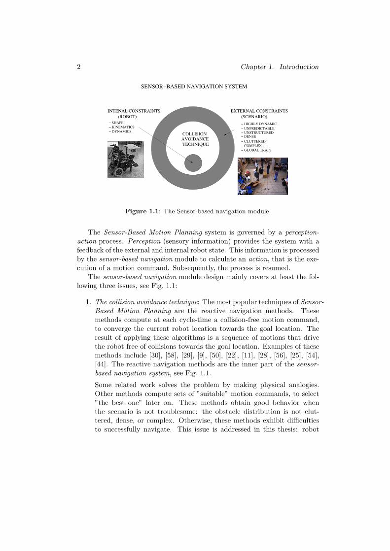
Figure 1.1: The Sensor-based navigation module.
The Sensor-Based Motion Planning system is governed by a perception-action process. Perception (sensory information) provides the system with afeedback of the external and internal robot state. This information is processedby the sensor-based navigation module to calculate an action, that is the exe-cution of a motion command. Subsequently, the process is resumed.
The sensor-based navigation module design mainly covers at least the fol-lowing three issues, see Fig. 1.1:
1. The collision avoidance technique: The most popular techniques of Sensor-Based Motion Planning are the reactive navigation methods. Thesemethods compute at each cycle-time a collision-free motion command,to converge the current robot location towards the goal location. Theresult of applying these algorithms is a sequence of motions that drivethe robot free of collisions towards the goal location. Examples of thesemethods include [30], [58], [29], [9], [50], [22], [11], [28], [56], [25], [54],[44]. The reactive navigation methods are the inner part of the sensor-based navigation system, see Fig. 1.1.
Some related work solves the problem by making physical analogies.Other methods compute sets of ”suitable” motion commands, to select”the best one” later on. These methods obtain good behavior whenthe scenario is not troublesome: the obstacle distribution is not clut-tered, dense, or complex. Otherwise, these methods exhibit difficultiesto successfully navigate. This issue is addressed in this thesis: robot
3
navigation in very dense, complex, and cluttered scenarios. Chapter 2presents a method called Nearness Diagram Navigation. By using thisreactive navigation method, navigation is successfully achieved in suchchallenge scenarios.
2. The internal constraints: These constraints are imposed by the vehiclespecific characteristics. There are at least three types of internal con-straints: (1) the robot shape, (2) the robot kinematic constraints, and(3) the robot dynamic constraints. These constraints are called internal,since they have to be considered in the design of the collision avoidancetechnique, see Fig. 1.1. (e.g. dealing with a car-like robot, the kinematicconstraints have to be taken into account in the design of the reactivenavigation method.) To address the specific vehicle shape, kinemat-ics, and dynamics is still a subject of research in Sensor-based MotionPlanning. However, some methods have been proposed dealing with theshape and kinematics [25], [56], [59], [60], [54], [62], [28], [22], [52], [47];and dealing with dynamics [56], [25], [13], [22], [62], [46]. Some of themaddress all of these constraints [52], [16], [62].
Mainly, related work addresses the kinematics or the dynamics by cal-culating sets of trajectories that comply with the kinematic or dynamicconstraints. One trajectory is selected with some criteria. Subsequently,a motion command, that drives the platform over the selected trajec-tory, is computed and executed by the vehicle. The limitation of theseapproaches is that usually, the reactive navigation method is designedfrom scratch to address the kinematics or the dynamics. There is a lotof literature that proposes particular solutions to address the kinematicand dynamic constraints in the Sensor-Based Motion Planning field. Butlittle attention has been paid to look for much wider solutions.
The Chapter 3 presents an under-constraint solution to address the robotshape, kinematics, and dynamics in the reactive navigation layer. Thissolution is used to extend the Nearness Diagram Navigation method toaddress these issues. Moreover, the usage of different sensors for navi-gation is explored. By using this framework, navigation is successfullyachieved in troublesome scenarios with non-circular robots that exhibitkinematic and dynamic constraints.
Chapter 4 presents a solution to address the kinematic constraints basedon a spatial representation called the Ego-Kinematic space. The robotkinematics is used in the construction of the spatial representation. Inthis space the robot moves as a free-flying object. Many existing reactive
4 Chapter 1. Introduction
navigation methods that do not address kinematics can be used in thisspace. As a consequence, the reactive method solution complies withthe kinematic constraints. This is an ample solution to address thekinematics in the Sensor-Based motion Planning field.
Chapter 5 addresses the dynamic constraints with a similar idea: to in-troduce the dynamics into the spatial representation, the Ego-Dynamicspace. With minor modifications, standard reactive navigation methodsthat do not address dynamics can be used in this space. As a conse-quence, the reactive method solution complies with the dynamic con-straints. This is an ample solution to address the dynamic constraintsinto the Sensor-Based Motion Planning field.
3. The external constraints: These constraints are imposed by the type ofscenario where the vehicle is moving. For most of the mobile roboticapplications, the environment nature is non-predictable, unstructured,and dynamic. Moreover, the environment structure can produce trapsituations or cyclic behaviors in the navigation systems that have to beavoided. These constraints are called external, since they do not di-rectly affect the design of the collision avoidance technique. However,an external layer, that process information to improve the pure reactivebehavior, is required (see Fig. 1.1). (e.g. moving the robot in a highlydynamic scenario requires a module to process the sensory information,in order to improve the reactive method behavior. Although, the re-active method might not be redesigned.) This issue has been mainlyaddressed in Sensor-Based Motion Planning breaking down the probleminto sub-problems: the collision avoidance technique, and the designof the external layer that improves the collision avoidance task. Eachof the modules works independently, but they interact to complete thenavigation task. Examples of these methods include [11], [59], [60], [13].
This issue has been mainly addressed by designing particular modulesin particular contexts. However, the instances of the modules are notgeneral, and no procedure is proposed to integrate the different modules.Chapter 6 presents some instances of the functionalities required to im-prove the method behavior in highly dynamic scenarios, and to avoidthe common trap situations. Nevertheless, an architecture is presentedallowing for integration of the base functionalities, and for module re-placement - indispensable to reutilize the technologies proposed in thisthesis for different robot and sensors.
This dissertation addresses all the issues that make up the design of the

5
Sensor-Based Motion Planning module: (1) the design of a sensor-based mo-tion planner. (2) Solutions for the sensor-based motion planning with shape,kinematic, and dynamic constraints. (3) Development of the modules requiredto improve the performance of the sensor-based motion planner. (4) Integra-tion of all the functionalities and the algorithms proposed in the dissertation.

6 Chapter 1. Introduction
Chapter 2
Nearness Diagram Navigation
2.1 Introduction
The safe motion generation is an important task in a typical indoor-outdoormobile robotic mission. Unfortunately the robot navigation in very cluttered,dense, and complex scenarios is still a robotic challenge. These scenarios arewhere the robots are usually required to move. Then, the robots are limitedto work in well-controlled environments.
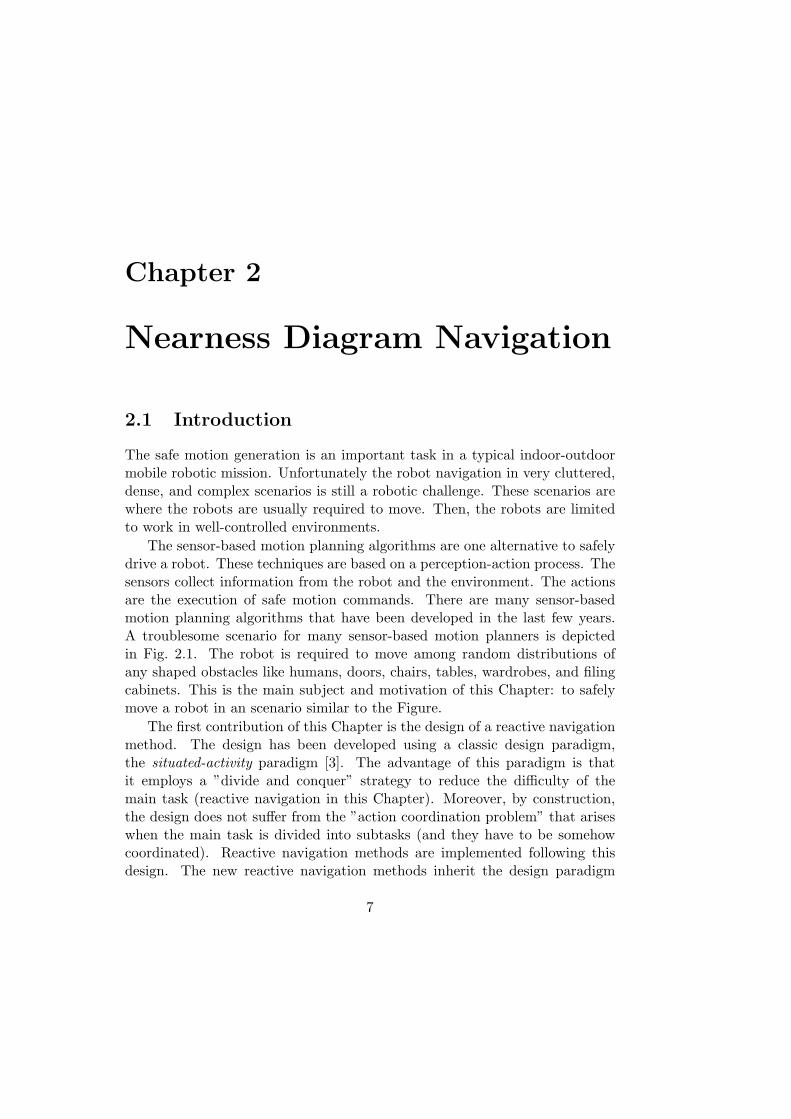
The sensor-based motion planning algorithms are one alternative to safelydrive a robot. These techniques are based on a perception-action process. Thesensors collect information from the robot and the environment. The actionsare the execution of safe motion commands. There are many sensor-basedmotion planning algorithms that have been developed in the last few years.A troublesome scenario for many sensor-based motion planners is depictedin Fig. 2.1. The robot is required to move among random distributions ofany shaped obstacles like humans, doors, chairs, tables, wardrobes, and filingcabinets. This is the main subject and motivation of this Chapter: to safelymove a robot in an scenario similar to the Figure.
The first contribution of this Chapter is the design of a reactive navigationmethod. The design has been developed using a classic design paradigm,the situated-activity paradigm [3]. The advantage of this paradigm is thatit employs a ”divide and conquer” strategy to reduce the difficulty of themain task (reactive navigation in this Chapter). Moreover, by construction,the design does not suffer from the ”action coordination problem” that ariseswhen the main task is divided into subtasks (and they have to be somehowcoordinated). Reactive navigation methods are implemented following thisdesign. The new reactive navigation methods inherit the design paradigm
7
8 Chapter 2. Nearness Diagram Navigation
Figure 2.1: Typical office environment. The snapshot was taken in a experimentperformed using the Robels system. The Nearness Diagram Navigation is the sensory-motor function that is driving the robot out of the office.
advantages. As a consequence, these methods must be able to solve morecomplex scenarios problems than other methods do.
The Nearness Diagram Navigation method has been implemented follow-ing the reactive navigation method design proposed. This reactive navigationmethod is a geometry-based implementation. The main contribution of thisimplementation is that it solves highly complex navigation problems. TheNearness Diagram Navigation successfully achieves navigation in very com-plex, dense, and cluttered scenarios. These scenarios present a high degree ofdifficulty for many existing methods. Experimental results with a real plat-form are presented to validate the method in these challenge environments.
This research was previously presented in [44].
The Chapter is organized as follows. After discussing the role of the re-active navigation and related work, Section 2.3 explains the situated-activitydesign methodology. Section 2.4 introduces the reactive navigation methoddesign. In Section 2.5 the Nearness Diagram Navigation method is imple-mented. Section 2.6 validates the research with experimentation on the realrobot. Section 2.7 discusses the contributions of our approach regarding othermethods, and in Section 2.8 the conclusions are drawn.
2.2. Preliminaries in Reactive Navigation 9
2.2 Preliminaries in Reactive Navigation
This Section discusses the application context where the reactive navigationmethods have better performance than techniques such as motion planning(Subsection 2.2.1). Related work is analyzed in order to place our approach,and to present the motivation for this work (Subsection 2.2.2).
2.2.1 The Reactive Navigation Problem
There are many ways to generate collision-free motion. Roughly, they can bedivided into those that are global, and based on a priori information (motionplanning). And into those that are local, and based on sensory information(reactive navigation methods). Both techniques have some differences thatjustify their usage depending on the application constraints. The context ofthis work is to move a robot in unknown, unstructured, and dynamic scenarios.
Motion planning techniques calculate a collision-free path between therobot and goal configurations (see [35] for a review). From the path, motioncommands are computed, and executed in real-time by the robot. The ad-vantage of these algorithms is that they provide a global solution for reachingthe goal. However, in unknown, unstructured, and dynamic scenarios the be-havior of the motion planning algorithms is diminished. Dealing with suddenenvironmental changes, new sensory perceptions need to be integrated into amodel, and continuous re-planning are required. Both tasks are time consum-ing, not complying with the real-time requirement. Besides, motion planningdo not solve some situations (e.g. a dynamic obstacle temporally locates it-self on top of the goal location). In these situations, the motion control loopcannot be closed, see Chapter 6.
The reactive navigation methods compute at each sample period onecollision-free motion command, to converge the current robot location towardsthe goal location. The result of applying these algorithms is a sequence ofmotions that drive the robot free of collisions towards the goal location. Oneof the advantages is that explicit models of the environment are not required.Another advantage is to not impose an expensive computational load. Thereactive methods are thus well-suited to deal with unknown, dynamic, andnon-predictable scenarios. The drawback is that these methods use a localfraction of the information available (sensory information). Then, it is difficultto obtain optimal solutions, and to avoid the trap situations.
The attention focuses on reactive navigation methods as they fitting inthe context of our application. The next Subsection presents related work tointroduce the motivation for this work.

10 Chapter 2. Nearness Diagram Navigation
2.2.2 Related Work
The related work is introduced grouped according to the perception-actionprocess carried out.
• There are methods that use a physical analogy to compute the motioncommands. Some mathematical equations are applied to the sensoryinformation. The solutions are transformed into motion commands (e.g.the potential field methods [30], [34], [58], [29], [9], [50], the perfumeanalogy [6], the fluid analogy [43], among others).
• There are methods that first compute some sets of motion commands.Next, a navigation strategy selects one motion command of these sets.Some methods calculate sets of steering angles [22], [11], [59], [28]. Oth-ers compute sets of velocity commands [56], [25], [13], [4].
• There are methods that calculate some form of high-level informationdescription from the sensory information. Then, a motion commandis computed, as opposed to being selected from a pre-calculated set.[54], and [29] formulate the concept of bubbles to describe parts of thefree space. A collision-free path, included within the bubbles, is usedto compute the motion commands. The Nearness Diagram Navigationmethod belongs to this group of approaches.
The motivation for this work is to develop a reactive navigation methodto achieve safe navigation in very dense, cluttered, and complex scenarios: atask that presents a high degree of difficulty for most of the methods mentionedabove.
2.3 The Situated-Activity Paradigm of Design
One of the goals of this Chapter is the design of a reactive navigation methodusing a classic design paradigm. This Section introduces the design paradigmselected, pointing out the advantages, difficulties, and requirements for itsapplication.
The situated-activity is a paradigm for designing behaviors in Robotics[3]. The paradigm is based on defining a set of situations that describe therelative state of the problem entities. Subsequently, an action is designed foreach situation. During the execution phase, perception is used to identify thecurrent situation, and the associated action is carried out.
2.4. The Reactive Navigation Method Design 11
This paradigm has some advantages for designing modules that executeaction-tasks with sensory information:
• The paradigm itself is a perception-action process.
• The paradigm utilizes a “divide and conquer” strategy to reduce thetask difficulty.
• The paradigm does not suffer the real-time action coordination problem.This problem arises when the main task is divided into sub-tasks toreduce the task difficulty 1.
The restriction for the application of the paradigm is to find a set ofsituations that effectively describes the task-problem to solve (as commonlypointed out [26]).
The usage of this paradigm has to comply with some design require-ments:
• The situations have to be identifiable from sensory perception, exclu-sive, and complete to represent the relative state of the problem entities.Moreover, the explosion in the number of situations needed has to beavoided.
• Each action design has to solve individually the task problem, in thecontext of each situation.
2.4 The Reactive Navigation Method Design
The goal of this Section is to understand the design of a reactive navigationmethod using the situated-activity paradigm. The Section presents the design,and analyzes the completion with the paradigm requirements.
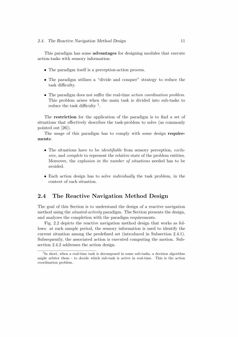
Fig. 2.2 depicts the reactive navigation method design that works as fol-lows: at each sample period, the sensory information is used to identify thecurrent situation among the predefined set (introduced in Subsection 2.4.1).Subsequently, the associated action is executed computing the motion. Sub-section 2.4.2 addresses the action design.
1In short, when a real-time task is decomposed in some sub-tasks, a decision algorithmmight arbiter them - to decide which sub-task is active in real-time. This is the actioncoordination problem.
12 Chapter 2. Nearness Diagram Navigation
LS2HSGR HSWR HSNR LS1
HSGR HSWR HSNR LS1 LS2
HSGRno
ACTIONS
HIGH SAFETY LOW SAFETY
Motion Commands (V,W)
Criterion 1
Criterion 2
Criterion 3
Criterion 4
Sensory Data Goal location
SITUATIONS
DECISIONTREE
Robot Location Data
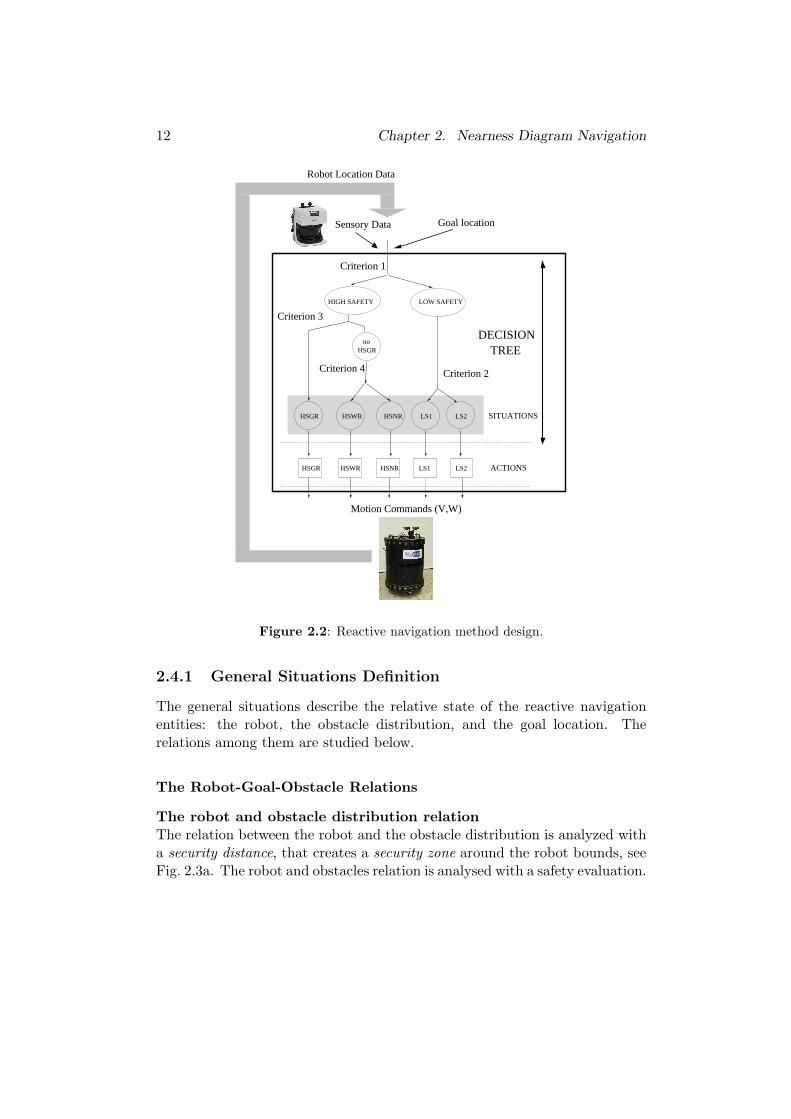
Figure 2.2: Reactive navigation method design.
2.4.1 General Situations Definition
The general situations describe the relative state of the reactive navigationentities: the robot, the obstacle distribution, and the goal location. Therelations among them are studied below.
The Robot-Goal-Obstacle Relations
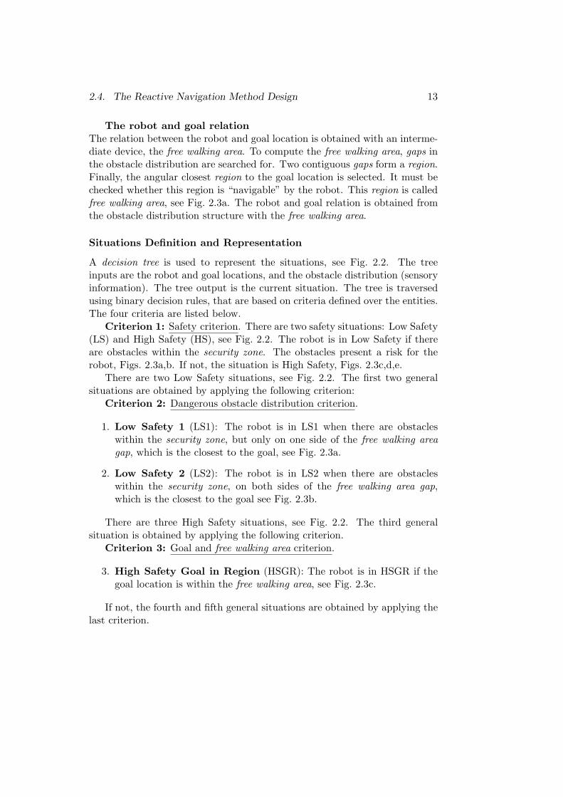
The robot and obstacle distribution relationThe relation between the robot and the obstacle distribution is analyzed witha security distance, that creates a security zone around the robot bounds, seeFig. 2.3a. The robot and obstacles relation is analysed with a safety evaluation.
2.4. The Reactive Navigation Method Design 13
The robot and goal relationThe relation between the robot and goal location is obtained with an interme-diate device, the free walking area. To compute the free walking area, gaps inthe obstacle distribution are searched for. Two contiguous gaps form a region.Finally, the angular closest region to the goal location is selected. It must bechecked whether this region is “navigable” by the robot. This region is calledfree walking area, see Fig. 2.3a. The robot and goal relation is obtained fromthe obstacle distribution structure with the free walking area.
Situations Definition and Representation
A decision tree is used to represent the situations, see Fig. 2.2. The treeinputs are the robot and goal locations, and the obstacle distribution (sensoryinformation). The tree output is the current situation. The tree is traversedusing binary decision rules, that are based on criteria defined over the entities.The four criteria are listed below.
Criterion 1: Safety criterion. There are two safety situations: Low Safety(LS) and High Safety (HS), see Fig. 2.2. The robot is in Low Safety if thereare obstacles within the security zone. The obstacles present a risk for therobot, Figs. 2.3a,b. If not, the situation is High Safety, Figs. 2.3c,d,e.
There are two Low Safety situations, see Fig. 2.2. The first two generalsituations are obtained by applying the following criterion:
Criterion 2: Dangerous obstacle distribution criterion.
1. Low Safety 1 (LS1): The robot is in LS1 when there are obstacleswithin the security zone, but only on one side of the free walking areagap, which is the closest to the goal, see Fig. 2.3a.
2. Low Safety 2 (LS2): The robot is in LS2 when there are obstacleswithin the security zone, on both sides of the free walking area gap,which is the closest to the goal see Fig. 2.3b.
There are three High Safety situations, see Fig. 2.2. The third generalsituation is obtained by applying the following criterion.
Criterion 3: Goal and free walking area criterion.
3. High Safety Goal in Region (HSGR): The robot is in HSGR if thegoal location is within the free walking area, see Fig. 2.3c.
If not, the fourth and fifth general situations are obtained by applying thelast criterion.
14 Chapter 2. Nearness Diagram Navigation
SIDE 1
ACTION
SIDE 2
GOAL X
GAP
FREE WALKINGAREA
CLOSESTGAP
SECURITY ZONE
GAP
ACTION
FREE WALKING
GAP
SIDE 1
AREAGOAL X
CLOSEST
SIDE 2
SECURITY ZONE
(a) (b)
GAP
GOAL X
FREE WALKING
GAP
ACTION
AREA
SECURITY ZONE
GOAL X
FREE WALKING
ACTION
GAP
GAP
AREACLOSEST
SECURITYZONE
X
ACTION
GAP
GAP
FREE WALKING
GOAL
AREA
CLOSEST
SECURITY ZONE
(c) (d) (e)
Figure 2.3: a) LS1 situation/action example. b) LS2 situation/action example.c) HSGR situation/action example. d) HSWR situation/action example. e)HSNRsituation/action example.
Criterion 4: Free walking area width criterion. A free walking area iswide if its angular width is larger than a given angle. If not, the free walkingarea is narrow.
4. High Safety Wide Region (HSWR): The robot is in HSWR if thegoal is not within the free walking area, but the free walking area is wide,see Fig. 2.3d.
5. High Safety Narrow Valley (HSNR): The robot is in HSNR if thegoal is not within the free walking area, but the free walking area isnarrow, see Fig. 2.3e.
Some conclusions regarding the definition and representation of these sit-uations are summarized next:
2.4. The Reactive Navigation Method Design 15
• The situations are identifiable from sensory perception. (When the sen-sory information is available as depth maps.)
• The situations are exclusive and complete. They are obtained from abinary decision tree.
• The situation definition avoids the explosion in the number of situations,because there are five. This comes from the fact that, the situation defi-nition does not depend on the resolution or size of the space considered.
Then, the definition and representation of the situations comply with therequirements imposed by the situated-activity paradigm, mentioned in Section2.3.
2.4.2 Action Design
This Subsection presents the action design guidelines:
1. Low Safety 1 (LS1): This action moves the robot away from the closestobstacle, while directing the robot towards the free walking area gapclosest to the goal, see Fig. 2.3a.
2. Low Safety 2 (LS2): This action keeps the robot at the same distancefrom the two closest obstacles, while moving the robot towards the freewalking area gap closest to the goal, see Fig. 2.3b.
3. High Safety Goal in Region (HSGR): This action drives the robotdirectly to the goal, see Fig. 2.3c.
4. High Safety Wide Region (HSWR): This action moves the robotalongside the obstacle, see Fig. 2.3d.
5. High Safety Narrow Region (HSNR): This action directs the robotthrough the central zone of the free walking area, see Fig. 2.3e.
Conclusions regarding the action design are next summarized. Each actionsolves individually the task problem, in the context of each situation: Avoidingobstacles while moving the robot towards the goal location. This is achievedin Low Safety and High Safety actions as follows:
• In Low Safety, both actions avoid the obstacles, while moving the robottowards the free walking area gap closest to the goal. This gap implicitlyhas information about the goal location.
16 Chapter 2. Nearness Diagram Navigation
• In High Safety, the actions drive the robot towards the goal, towardsthe free walking area gap closest to the goal, or towards the central zoneof the free walking area. Then, these actions explicitly or implicitlydrive the robot towards the goal location. The robot is not in danger ofcollision, so there is no need to avoid obstacles.
Then, the actions design comply with the requirements imposed by thesituated-activity paradigm, mentioned in Section 2.3.
There are some points worth mentioning here:
1. The reactive navigation method design is described in symbolic level.Different implementations of this design lead to new reactive navigationmethods. Learning techniques, Fuzzy sets, Potential Field implementa-tions, optimization techniques and other tools may be used to implementthe design. The next Section presents a geometry-based implementation.
2. Any reactive navigation method implemented following the proposeddesign simplifies the reactive navigation problem (by a “divide and con-quer” strategy based on situations). So, a good implementation mightsolve more difficult navigation problems than other existing methods,that use a unique navigation heuristic, do. Besides, the design is flexi-ble. New situations might be defined to reduce the difficulty even more.
3. The design does not suffer from the ”action coordination problem”. Thesub-tasks are self-coordinated, because the general situations are com-plete and exclusive. Only one situation can be selected at each time, andthus, only one action is executed.
Summarizing, this Section has presented the design of a reactive navigationmethod using the situated-activity paradigm. The Section also demonstratedthat the situations, and the associated actions, comply with the requirementsimposed by the paradigm.
2.5 The Nearness Diagram Navigation (ND)
This Section presents a geometry-based implementation of the design calledthe Nearness Diagram Navigation.
The attention is focused on a circular (with radius R) holonomic robotmoving over a flat surface. The Workspace W is IR2. A point x = (x, y) ∈ IR2
is a location of the robot. The space of motion commands is three-dimensional.

2.5. The Nearness Diagram Navigation (ND) 17
Let (v,w) be a motion command. Let v = (vm, θ) be the translational velocity,and let w be the rotational velocity.
The sensory information is supposed to be depth point maps for two rea-sons: (1) maintaining the sensor as general as possible - the great majorityof sensory information can be processed and then reduced to points, and (2)avoiding the use of structured information (as lines, polygons, etc), that oth-erwise can be used if it is available. Let L be a list of the N obstacle pointsperceived at each time.
Fig. 2.2 depicts the ND method design that works as follows: at each sam-ple period T the sensory information is used to identify the current situationamong the predefined set (introduced in Subsection 2.5.1). Subsequently, theassociated action is executed computing the motion commands, (v,w). Theactions are control laws presented in Subsection 2.5.2.
2.5.1 Information Representation and General Situations
This Subsection introduces the tools used to analyze the sensory information:the Nearness Diagrams. Subsequently, the robot location, obstacle distribu-tion, and goal location relations are used to define the general situations.
Nearness Diagram Definition
The ND divides the space in sectors whose centre is over the robot centre.Let n be the number of sectors (n = 144 in our implementation, so 2.5◦ is theangle of each sector). Notice that in the robot reference, the bisector of the n
2sector is 0◦, of the n
4 is π2 , and of the 3n
4 is −π2 .
Let δi(x, L) be the function that computes the distance from the robotcentre to the closest obstacle point in sector i. δi(x, L) = 0 when there areno obstacles in sector i. max(δi(x, L)) = dmax, where dmax is the maximumrange of the sensor. Then, let D = {di = δi(x, L), i = 1 . . . n} be the list ofthe minimum obstacle distances to the robot centre in each sector.
Definition 1 Nearness Diagram from the central Point (PND)
PND : IR2 ×D → {IR+ ∪ {0}}n
(x, di) → {PNDi(x, di)}n
if di > 0, PNDi(x, di) = dmax + 2R− di
else PNDi(x, di) = 0
18 Chapter 2. Nearness Diagram Navigation
Definition 2 Nearness Diagram from the Robot bounds (RND)
RND : IR2 ×D → {IR+ ∪ {0}}n
(x, di) → {RNDi(x, di)}n
if di > 0, RNDi(x, di) = dmax + Ei − di
else RNDi(x, di) = 0
where
• E: function that depends on the robot geometry. The function Ei is the robotradius, R, for a circular robot 2.
The PND represents the nearness of the obstacles from the robot centre.The RND represents the nearness of the obstacles from the robot boundary.Some PND and RND diagrams are illustrated in Fig. 2.4. From now on,PNDi ≡ PNDi(x, di) and RNDi ≡ RNDi(x, di).
The Robot-Goal-Obstacle Relations
The relations among the robot, the obstacle distribution, and the goal areanalyzed by using these diagrams.
The robot and obstacle distribution relationThe relation between the robot and the obstacle distribution is obtained with asafety evaluation. This evaluation is made with the RND, because it representsthe nearness of the obstacles from the robot bounds. Let the security distancebe the minimum obstacle admissible distance, ds, to the robot bounds. Asecurity nearness is computed by ns = dmax − ds, and used in the RND toevaluate the robot safety, see Fig. 2.4c.
The robot and goal relationThe relation between the robot and the goal location is obtained from a highlevel device called free walking area. It is computed from the PND, since itrepresents the nearness from the obstacles to the robot centre. The PNDanalysis is carried out in three stages. First, gaps are identified. From thesegaps, regions are obtained, and finally one region is selected: the free walkingarea, see Fig. 2.4a.
1. Gaps: First, gaps in the obstacle distribution are identified searching fordiscontinuities in the PND.
2If the robot is not circular, Ei is the distance from the robot centre to the robot boundsin sector i.
2.5. The Nearness Diagram Navigation (ND) 19
GOALx
SECURITYDISTANCE
ROBOTORIENTATION
REGION 2
FREE WALKINGAREA
GAP 1
GAP 2
GAP 3
GAP 4
GAP 5
GAP 6
REGION 1
(a)
0 20 40 60 80 100 120 1400
0.5
1
1.5
2
2.5
3
3.5
4
SECTORS
PND
VALLEY 1 VALLEY 2VALLEYSELECTED
ROBOT
ORIENTATION
Sgoal
1
2
3
4
56
0 20 40 60 80 100 120 1400
0.5
1
1.5
2
2.5
3
3.5
4
SECTORS
RND
SECURITYNEARNESS
(b) (c)
Figure 2.4: a) Gaps, regions, and free walking area. b) PND. c) RND. The followingvalues were set: R = 0.3m, dmax = 3m, ds = 0.3m.
A discontinuity exists between two sectors (i, j) if they are adjacent3,and their PND value differs by more than 2R (robot diameter), that is|PNDi − PNDj | > 2R. Fig. 2.4a depicts the gaps searched for. Theyare identified by discontinuities in the PND, see Fig. 2.4b. Notice thatthe robot diameter is used because only gaps where the robot fits aresearched for.
Two types of discontinuities are distinguished. When there is a discon-
3The adjacent sectors to i are i − 1 and i + 1. It is assumed that in all the operationsamong sectors the mod(∗, n) function is used. Thus, if i = n then i = 0. This gives continuityto the diagrams.
20 Chapter 2. Nearness Diagram Navigation
tinuity between two sectors (i, j), then: if PNDi > PNDj the disconti-nuity is a rising discontinuity from j to i, and a descending discontinuityfrom i to j.
Regions: Two contiguous gaps form a region. Regions are identifiedsearching for valleys in the PND.
Let be a valley a non empty set of sectors, S = {i + p}p=0,···,r withn > r ≥ 0, that satisfies the following conditions:
(a) There are no discontinuities between adjacent sectors of S.
(b) There exist two discontinuities:|PNDi−1 − PNDi| > 2R AND |PNDi+p − PNDi+p+1| > 2R
(c) One of these discontinuities is a rising discontinuity from i to i− 1or from i + p to i + p + 1 :PNDi−1 > PNDi OR PNDi+p+1 > PNDi+p
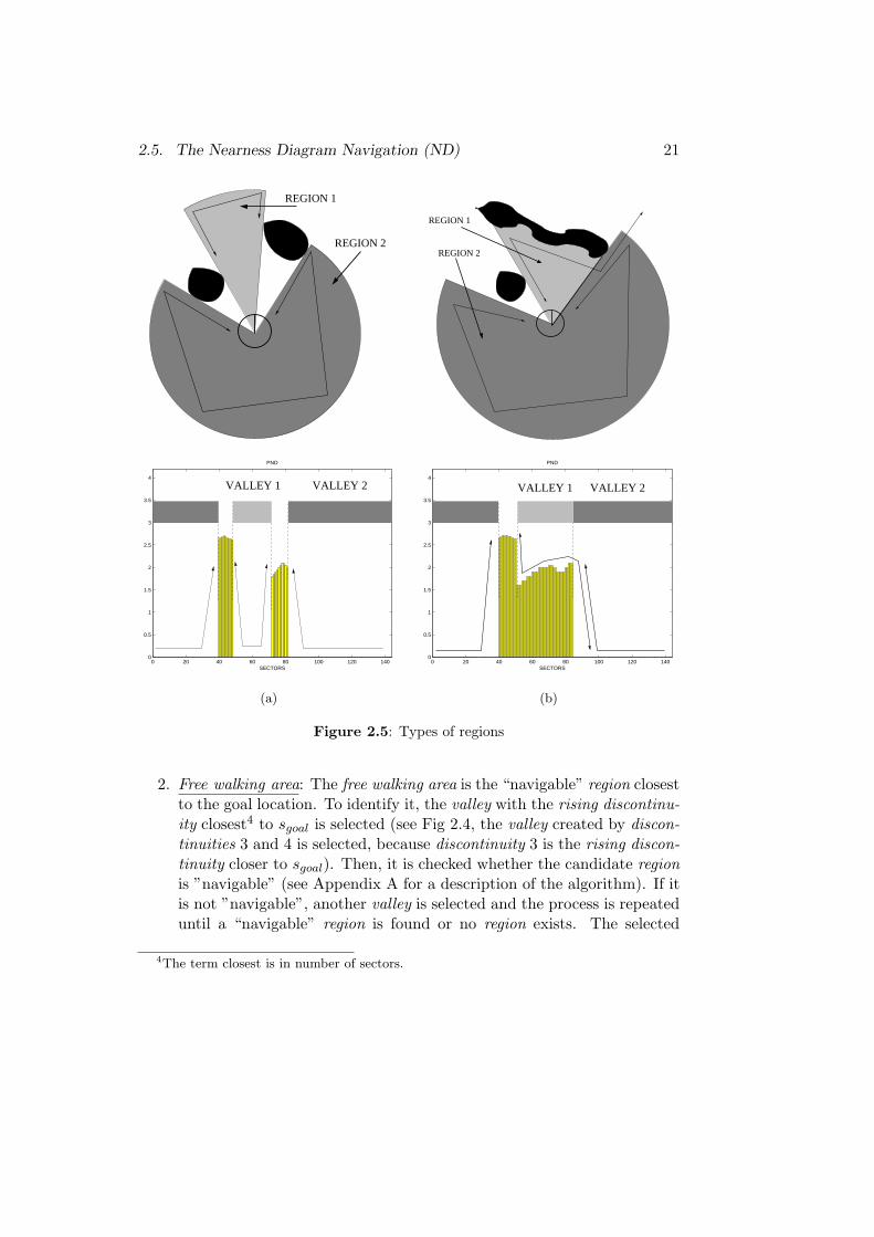
Fig. 2.5 depicts some regions and the valleys identified in the PND.There are not gaps within a region. Then, there cannot be discontinuitieswithin a valley (condition (a)). A region has one gap at each side. Then,a valley has two discontinuities in the extreme sectors i and i+p, (i−1, i)and (i+p, i+p+1). The sectors i−1 and i+p+1 do not belong to thevalley, but are adjacent to i and i+p respectively (condition (b)). Finally,at least one of the discontinuities of the valley has to be rising (condition(c)). Fig. 2.5a depicts two regions that are identified by valleys createdby two rising discontinuities. Valley1 in Fig. 2.5b is created by onedescending and one rising discontinuity. Thus, it identifies the region1.The number of rising discontinuities structurally differs the two types ofregions considered (e.g. in Fig. 2.5b, region2 is identified by valley2 thathas two rising discontinuities, however region1 is identified by valley1that has only one rising discontinuity).
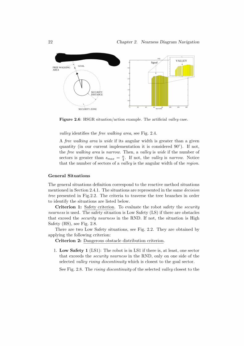
A special case occurs when the goal is between an obstacle and the robot.The sector that contains the goal location, sgoal, could not belong to avalley. However, it is desirable that when this condition arises, the goalwas within a region. Thus, when this situation is detected, the PNDsgoal
value is set equal to zero. This creates an artificial valley in the goalsector, that is, the goal is within a region. This case is illustrated inFig. 2.6. Another special case is when there are not obstacles. Then allthe sectors form the valley.
2.5. The Nearness Diagram Navigation (ND) 21
REGION 2
REGION 1
REGION 1
REGION 2
0 20 40 60 80 100 120 1400
0.5
1
1.5
2
2.5
3
3.5
4
SECTORS
PND
VALLEY 1 VALLEY 2
0 20 40 60 80 100 120 1400
0.5
1
1.5
2
2.5
3
3.5
4
SECTORS
PND
VALLEY 1 VALLEY 2
(a) (b)
Figure 2.5: Types of regions
2. Free walking area: The free walking area is the “navigable” region closestto the goal location. To identify it, the valley with the rising discontinu-ity closest4 to sgoal is selected (see Fig 2.4, the valley created by discon-tinuities 3 and 4 is selected, because discontinuity 3 is the rising discon-tinuity closer to sgoal). Then, it is checked whether the candidate regionis ”navigable” (see Appendix A for a description of the algorithm). If itis not ”navigable”, another valley is selected and the process is repeateduntil a “navigable” region is found or no region exists. The selected
4The term closest is in number of sectors.
22 Chapter 2. Nearness Diagram Navigation
SECURITY ZONE
FREE WALKINGAREA
GOAL X
DISTANCESECURITY
0 20 40 60 80 100 120 1400
0.5
1
1.5
2
2.5
3
3.5
4
SECTORS
PND
50 55 60 65 70 75 80
2.2
2.3
2.4
2.5
2.6
2.7
2.8
2.9
3
3.1
3.2
SECTORS
PND
VALLEYSgoal
Figure 2.6: HSGR situation/action example. The artificial valley case.
valley identifies the free walking area, see Fig. 2.4.
A free walking area is wide if its angular width is greater than a givenquantity (in our current implementation it is considered 90◦). If not,the free walking area is narrow. Then, a valley is wide if the number ofsectors is greater than smax = n
4 . If not, the valley is narrow. Noticethat the number of sectors of a valley is the angular width of the region.
General Situations
The general situations definition correspond to the reactive method situationsmentioned in Section 2.4.1. The situations are represented in the same decisiontree presented in Fig.2.2. The criteria to traverse the tree branches in orderto identify the situations are listed below.
Criterion 1: Safety criterion. To evaluate the robot safety the securitynearness is used. The safety situation is Low Safety (LS) if there are obstaclesthat exceed the security nearness in the RND. If not, the situation is HighSafety (HS), see Fig. 2.8.
There are two Low Safety situations, see Fig. 2.2. They are obtained byapplying the following criterion:
Criterion 2: Dangerous obstacle distribution criterion.
1. Low Safety 1 (LS1): The robot is in LS1 if there is, at least, one sectorthat exceeds the security nearness in the RND, only on one side of theselected valley rising discontinuity which is closest to the goal sector.
See Fig. 2.8. The rising discontinuity of the selected valley closest to the
2.5. The Nearness Diagram Navigation (ND) 23
goal sector (sgoal), is si (see the PND). Then, there are sectors exceedingthe security nearness only on one side of si in the RND .
2. Low Safety 2 (LS2): The robot is in LS2 if there is, at least, one sectorthat exceeds the security nearness in the RND, on both sides of theselected valley rising discontinuity which is closest to the goal sector.
See Fig. 2.8. The rising discontinuity of the selected valley closest to thegoal sector (sgoal), is si (see the PND). Then, there are sectors exceedingthe security nearness on both sides of si in the RND.
There are three High Safety situations, see Fig. 2.2. The third generalsituation is obtained by applying the following criterion:
Criterion 3: Goal and free walking area criterion.
3. High Safety Goal in Region (HSGR): The robot is in HSGR if thegoal sector belongs to the selected valley.
See Fig. 2.8. The goal sector (sgoal) belongs to the selected valley, see thePND. Notice that no sector exceeds the security nearness in the RND.
If not, the fourth and fifth general situations are obtained by applying thelast criterion.
Criterion 4: Free walking area width criterion.
4. High Safety Wide Region (HSWR): The robot is in HSWR if thegoal sector does not belong to the selected valley, but the valley is wide.
See Fig. 2.8. The goal sector (sgoal) do not belong to the selected valleythat is wide (the number of sectors of the valley is 102 > n
4 = 36), see thePND. Notice that no sector exceeds the security nearness in the RND.
5. High Safety Narrow Region (HSNR): The robot is in HSNR ifthe goal sector does not belong to the selected valley, but the valley isnarrow.
See Fig. 2.8. The goal sector (sgoal) do not belong to the selected valleythat is narrow (the number of sectors of the valley is 13 < n
4 = 36),see the PND. Notice that no sector exceeds the security nearness in theRND.
This Section has described the tools used to represent the sensory infor-mation, and the definition and identification of the general situations.
24 Chapter 2. Nearness Diagram Navigation
2.5.2 Associated Actions
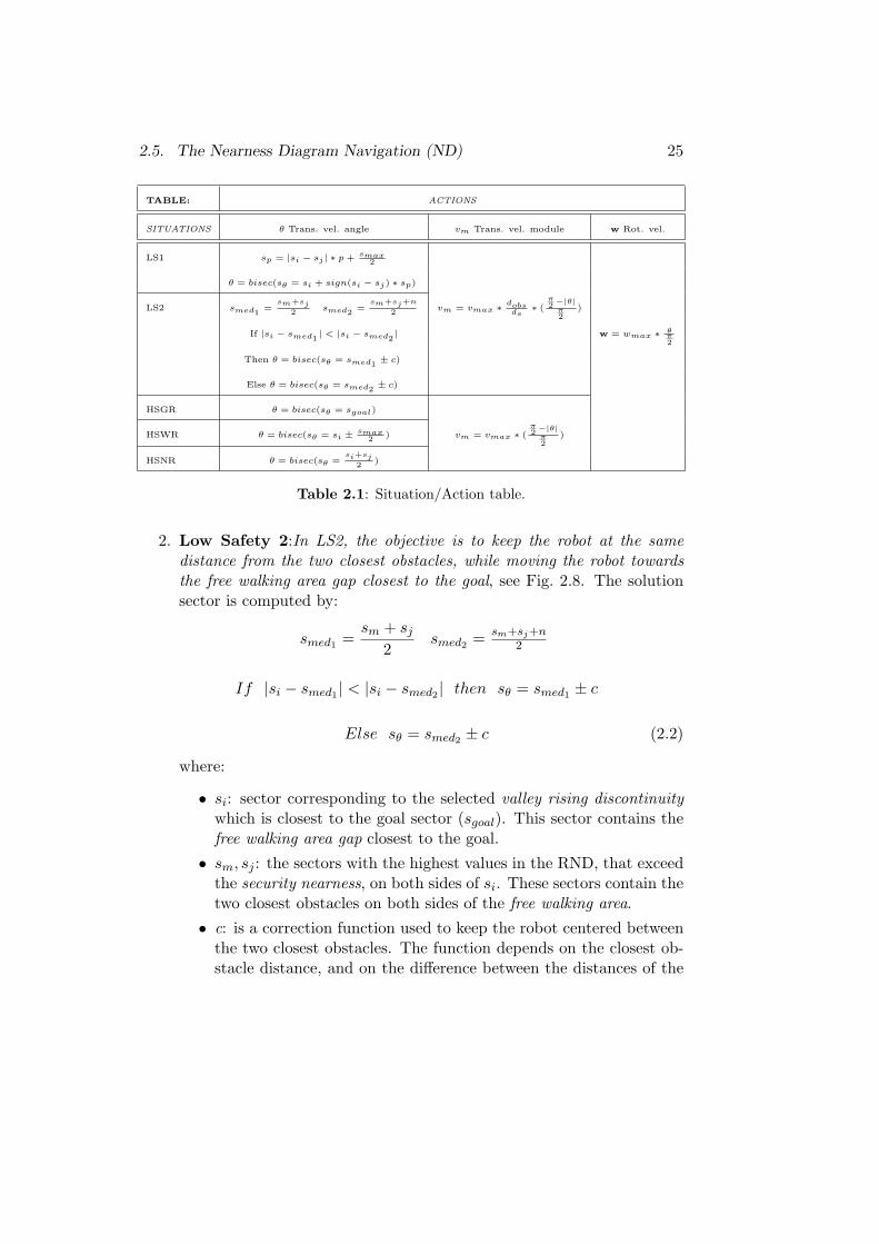
This Subsection introduces the implementation of the actions associated withthe general situations. The objective is to find simple control laws that producethe desired behavior associated with the situation identified (following thereactive method design, see Section 2.4.2). The actions compute the motioncommands (vm, θ,w). The action implementation is summarized in Table I.
Translational Velocity Direction (θ)
A solution sector, sθ ∈ IR, is calculated for each situation. The direction ofmotion θ (translational velocity direction) is the bisector of sθ. As sθ ∈ IR, anydirection of motion can be assigned θ ∈ [−π, π]. For a realistic implementationof the method, instantaneous backwards motion is prohibited (θ ∈ [−π/2, π/2],sθ ∈ [n4 , 3∗n
4 ]).Translational velocity direction in Low Safety
In Low Safety the robot is in danger of colliding because there are obstacleswithin the security zone. The robot must be brought to a secure situation.
1. Low Safety 1: In LS1, the objective is to move the robot away from theclosest obstacle, while directing the robot towards the free walking areagap closest to the goal, see Fig. 2.8. The solution sector, sθ, is calculatedby:
sp = |si − sj | ∗ p + smax2
sθ = si + sign(si − sj) ∗ sp (2.1)
where:
• si: sector corresponding to the selected valley rising discontinuitywhich is closest to the goal sector (sgoal). This sector contains thefree walking area gap closest to the goal.
• sj : sector with the highest value in the RND, that exceeds thesecurity nearness, on one side of si. This sector contains the closestobstacle point.
• p: experimentally tuned parameter. Its value depends on the tran-sitions among the general situations, to ensure a smooth behavioramong them. The parameter acts as an adaptable proportionalcontroller. In the current implementation p ∈ [1.5, 2.5].
2.5. The Nearness Diagram Navigation (ND) 25
TABLE: ACTIONS
SITUATIONS θ Trans. vel. angle vm Trans. vel. module w Rot. vel.
LS1 sp = |si − sj | ∗ p + smax2
θ = bisec(sθ = si + sign(si − sj) ∗ sp)
LS2 smed1 =sm+sj
2 smed2 =sm+sj+n
2 vm = vmax ∗ dobsds
∗ (π2 −|θ|
π2
)
If |si − smed1 | < |si − smed2 | w = wmax ∗ θπ2
Then θ = bisec(sθ = smed1 ± c)
Else θ = bisec(sθ = smed2 ± c)
HSGR θ = bisec(sθ = sgoal)
HSWR θ = bisec(sθ = si ± smax2 ) vm = vmax ∗ (
π2 −|θ|
π2
)
HSNR θ = bisec(sθ =si+sj
2 )
Table 2.1: Situation/Action table.
2. Low Safety 2:In LS2, the objective is to keep the robot at the samedistance from the two closest obstacles, while moving the robot towardsthe free walking area gap closest to the goal, see Fig. 2.8. The solutionsector is computed by:
smed1 =sm + sj
2smed2 = sm+sj+n
2
If |si − smed1 | < |si − smed2 | then sθ = smed1 ± c
Else sθ = smed2 ± c (2.2)
where:
• si: sector corresponding to the selected valley rising discontinuitywhich is closest to the goal sector (sgoal). This sector contains thefree walking area gap closest to the goal.
• sm, sj : the sectors with the highest values in the RND, that exceedthe security nearness, on both sides of si. These sectors contain thetwo closest obstacles on both sides of the free walking area.
• c: is a correction function used to keep the robot centered betweenthe two closest obstacles. The function depends on the closest ob-stacle distance, and on the difference between the distances of the

26 Chapter 2. Nearness Diagram Navigation
two closest obstacles. This quantity, c, is added or subtracted dueto the sector that contains closest obstacle.
Translational velocity direction in High SafetyIn High Safety the robot is not in danger of colliding. Thus, the robot moveswithin the free walking area.
3. High Safety Goal in Region: In HSGR the objective is to drive therobot directly to the goal, see Fig. 2.8. The solution sector is calculatedby sθ = sgoal.
The goal location is explicitly used to compute the motion commandsonly in this situation. Notice that the robot is not in danger of colliding,and the goal is within the free walking area. This situation is not dan-gerous for the robot, and does not appear to exhibit complexity. Fig. 2.6depicts the special case where an artificial valley is created preservingthe HSGR situation.
4. High Safety Wide Region: In HSWR the objective is to cause a mo-tion alongside the obstacle, see Fig. 2.8. The solution sector is calculatedby:
sθ = si ± smax2 (2.3)
where:
• si: sector corresponding to the selected valley rising discontinuitywhich is closest to the goal sector (sgoal). This sector contains thefree walking area gap closest to the goal.
5. High Safety Narrow Region: In HSNR the objective is to direct therobot through the central zone of the free walking area, see Fig. 2.8.
sθ =si + sj
2(2.4)
where:
• si, sj : sectors of the two discontinuities of the selected valley. Thesesectors contain the two gaps of the free walking area.
2.5. The Nearness Diagram Navigation (ND) 27
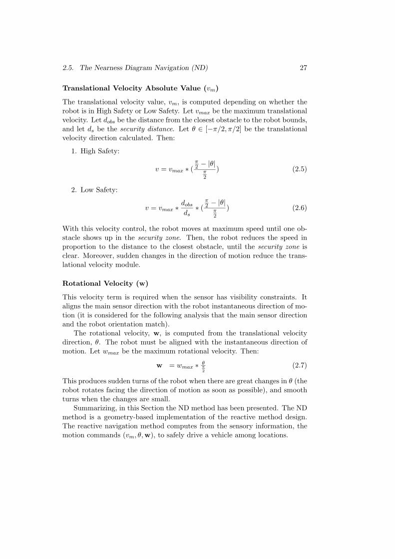
Translational Velocity Absolute Value (vm)
The translational velocity value, vm, is computed depending on whether therobot is in High Safety or Low Safety. Let vmax be the maximum translationalvelocity. Let dobs be the distance from the closest obstacle to the robot bounds,and let ds be the security distance. Let θ ∈ [−π/2, π/2] be the translationalvelocity direction calculated. Then:
1. High Safety:
v = vmax ∗ (π2 − |θ|
π2
) (2.5)
2. Low Safety:
v = vmax ∗ dobs
ds∗ (
π2 − |θ|
π2
) (2.6)
With this velocity control, the robot moves at maximum speed until one ob-stacle shows up in the security zone. Then, the robot reduces the speed inproportion to the distance to the closest obstacle, until the security zone isclear. Moreover, sudden changes in the direction of motion reduce the trans-lational velocity module.
Rotational Velocity (w)
This velocity term is required when the sensor has visibility constraints. Italigns the main sensor direction with the robot instantaneous direction of mo-tion (it is considered for the following analysis that the main sensor directionand the robot orientation match).
The rotational velocity, w, is computed from the translational velocitydirection, θ. The robot must be aligned with the instantaneous direction ofmotion. Let wmax be the maximum rotational velocity. Then:
w = wmax ∗ θπ2
(2.7)
This produces sudden turns of the robot when there are great changes in θ (therobot rotates facing the direction of motion as soon as possible), and smoothturns when the changes are small.
Summarizing, in this Section the ND method has been presented. The NDmethod is a geometry-based implementation of the reactive method design.The reactive navigation method computes from the sensory information, themotion commands (vm, θ,w), to safely drive a vehicle among locations.
28 Chapter 2. Nearness Diagram Navigation
2.6 Implementation and Experimental Results
The goal of this Section is to experimentally validate the ND method.
2.6.1 The Mobile Platform
The ND method has been tested on a Nomadic XR4000 at LAAS-CNRS,France. The robot is equipped with a SICK 2-D laser rangefinder. For furtherdetails about the platform and sensor see Appendix E. The sample period ofthe ND method is around 125msec on the on-board Pentium II. In the currentimplementation, a short-time memory built with the last 20 laser measure-ments (361 × 20 points) is used. The maximum translational velocity is setto vmax = 0.3 m
sec , and the maximum rotational one is set to wmax = 1.57 radsec .
These velocity limits were selected due to the potential applications of themethod: safe motion in indoor human environments. These scenarios exhibita high density of obstacles and the robot must work with humans aroundpreserving their safety, see Fig. 2.1.
2.6.2 Experimental Results
Three experiments using the real platform are discussed next. In all the exper-iments the scenario was unknown. The environment might be unstructured,dynamic, and non predictable. Only the goal location was available in ad-vance. These circumstances justify the usage of a reactive navigation methodto move the robot, see Subsection 2.2.1.
The experiments were designed to verify that the ND method complieswith the motivation of this work: to safely drive a robot in very dense, clut-tered, and complex scenarios. The experiments will also allow for discussion ofthe method technical contributions in the next Section, which are summarizedas follows: (1) avoiding trap situations due to the perceived environment struc-ture (e.g. U-shape obstacles, two very close obstacles); (2) generating stableand oscillation-free motion; (3) selecting motion directions towards obstacles;(4) exhibiting a high goal insensitivity - i.e. to be able to choose motion direc-tions far away from the goal direction; (5) selecting regions of motion using arobust ”navigability” criterion.
For each experiment an upper view is shown: the robot trajectory and allthe laser points perceived, see Fig. 2.9a. The robot velocity profiles are alsoillustrated, see Fig. 2.9b. Some snapshots have been selected for better under-standing of the robot motion - the floor tiles are 10cm square and the robot
2.6. Implementation and Experimental Results 29
0 10 20 30 40 50 600
1
2
3
4
5
6Situations
Time (sec)
Situ
atio
ns
LS2
LS1
HSWR
HSNR
HSGV
SITUATIONS
0 50 100 150 2000
1
2
3
4
5
6Situations
Time (sec)
Situ
atio
ns
LS2
LS1
HSWR
HSNR
HSGR
SITUATIONS
(a) (b)
0 10 20 30 40 50 60 700
1
2
3
4
5
6Situations
Time (sec)
Situ
atio
ns
LS2
LS1
HSWR
HSNR
HSGV
SITUATIONS
(c)
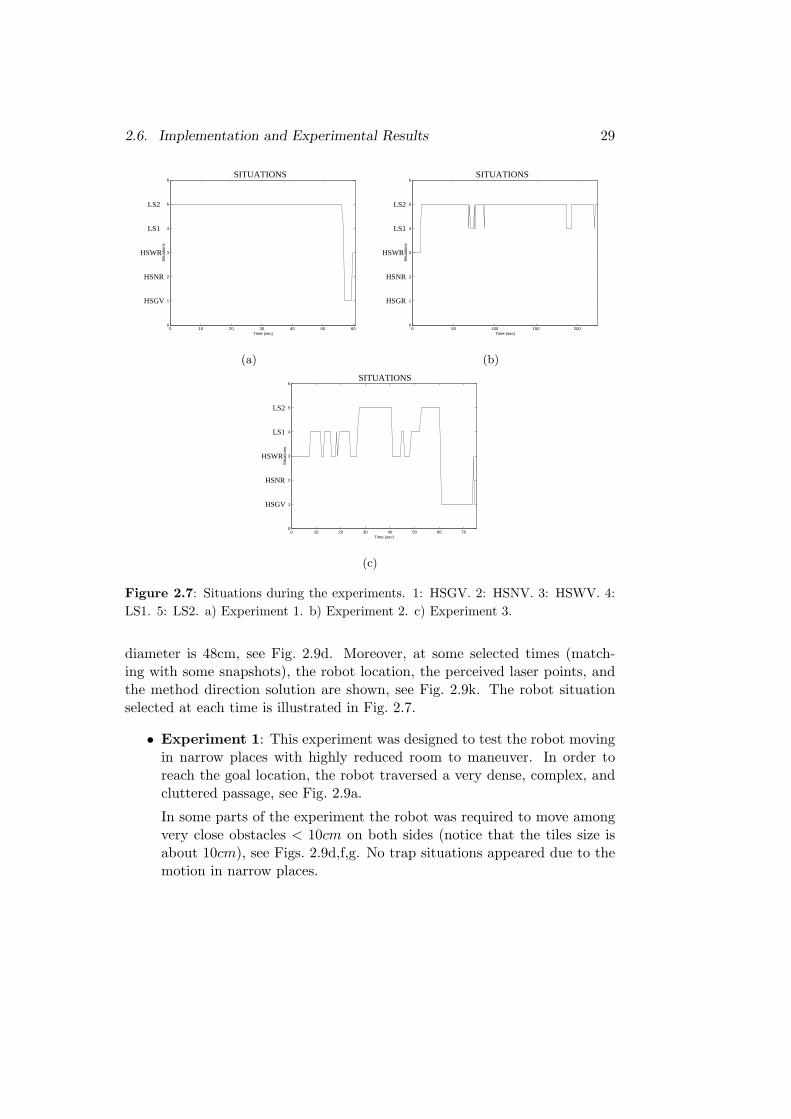
Figure 2.7: Situations during the experiments. 1: HSGV. 2: HSNV. 3: HSWV. 4:LS1. 5: LS2. a) Experiment 1. b) Experiment 2. c) Experiment 3.
diameter is 48cm, see Fig. 2.9d. Moreover, at some selected times (match-ing with some snapshots), the robot location, the perceived laser points, andthe method direction solution are shown, see Fig. 2.9k. The robot situationselected at each time is illustrated in Fig. 2.7.
• Experiment 1: This experiment was designed to test the robot movingin narrow places with highly reduced room to maneuver. In order toreach the goal location, the robot traversed a very dense, complex, andcluttered passage, see Fig. 2.9a.
In some parts of the experiment the robot was required to move amongvery close obstacles < 10cm on both sides (notice that the tiles size isabout 10cm), see Figs. 2.9d,f,g. No trap situations appeared due to themotion in narrow places.
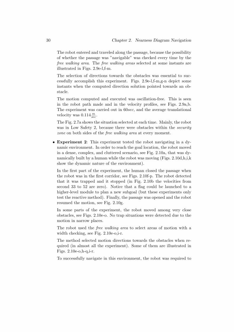
30 Chapter 2. Nearness Diagram Navigation
The robot entered and traveled along the passage, because the possibilityof whether the passage was ”navigable” was checked every time by thefree walking area. The free walking areas selected at some instants areillustrated in Figs. 2.9e-l,f-m.
The selection of directions towards the obstacles was essential to suc-cessfully accomplish this experiment. Figs. 2.9e-l,f-m,g-n depict someinstants when the computed direction solution pointed towards an ob-stacle.
The motion computed and executed was oscillation-free. This is seenin the robot path made and in the velocity profiles, see Figs. 2.9a,b.The experiment was carried out in 60sec, and the average translationalvelocity was 0.114 m
sec .
The Fig. 2.7a shows the situation selected at each time. Mainly, the robotwas in Low Safety 2, because there were obstacles within the securityzone on both sides of the free walking area at every moment.
• Experiment 2: This experiment tested the robot navigating in a dy-namic environment. In order to reach the goal location, the robot movedin a dense, complex, and cluttered scenario, see Fig. 2.10a, that was dy-namically built by a human while the robot was moving (Figs. 2.10d,h,i,kshow the dynamic nature of the environment).
In the first part of the experiment, the human closed the passage whenthe robot was in the first corridor, see Figs. 2.10f-p. The robot detectedthat it was trapped and it stopped (in Fig. 2.10b the velocities fromsecond 33 to 52 are zero). Notice that a flag could be launched to ahigher-level module to plan a new subgoal (but these experiments onlytest the reactive method). Finally, the passage was opened and the robotresumed the motion, see Fig. 2.10g.
In some parts of the experiment, the robot moved among very closeobstacles, see Figs. 2.10e-o. No trap situations were detected due to themotion in narrow places.
The robot used the free walking area to select areas of motion with awidth checking, see Fig. 2.10e-o,i-r.
The method selected motion directions towards the obstacles when re-quired (in almost all the experiment). Some of them are illustrated inFigs. 2.10e-o,h-q,i-r.
To successfully navigate in this environment, the robot was required to
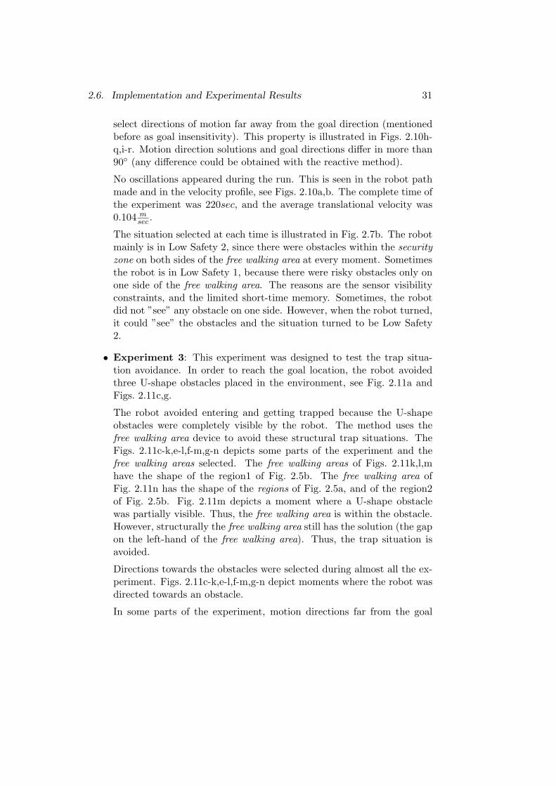
2.6. Implementation and Experimental Results 31
select directions of motion far away from the goal direction (mentionedbefore as goal insensitivity). This property is illustrated in Figs. 2.10h-q,i-r. Motion direction solutions and goal directions differ in more than90◦ (any difference could be obtained with the reactive method).
No oscillations appeared during the run. This is seen in the robot pathmade and in the velocity profile, see Figs. 2.10a,b. The complete time ofthe experiment was 220sec, and the average translational velocity was0.104 m
sec .
The situation selected at each time is illustrated in Fig. 2.7b. The robotmainly is in Low Safety 2, since there were obstacles within the securityzone on both sides of the free walking area at every moment. Sometimesthe robot is in Low Safety 1, because there were risky obstacles only onone side of the free walking area. The reasons are the sensor visibilityconstraints, and the limited short-time memory. Sometimes, the robotdid not ”see” any obstacle on one side. However, when the robot turned,it could ”see” the obstacles and the situation turned to be Low Safety2.
• Experiment 3: This experiment was designed to test the trap situa-tion avoidance. In order to reach the goal location, the robot avoidedthree U-shape obstacles placed in the environment, see Fig. 2.11a andFigs. 2.11c,g.
The robot avoided entering and getting trapped because the U-shapeobstacles were completely visible by the robot. The method uses thefree walking area device to avoid these structural trap situations. TheFigs. 2.11c-k,e-l,f-m,g-n depicts some parts of the experiment and thefree walking areas selected. The free walking areas of Figs. 2.11k,l,mhave the shape of the region1 of Fig. 2.5b. The free walking area ofFig. 2.11n has the shape of the regions of Fig. 2.5a, and of the region2of Fig. 2.5b. Fig. 2.11m depicts a moment where a U-shape obstaclewas partially visible. Thus, the free walking area is within the obstacle.However, structurally the free walking area still has the solution (the gapon the left-hand of the free walking area). Thus, the trap situation isavoided.
Directions towards the obstacles were selected during almost all the ex-periment. Figs. 2.11c-k,e-l,f-m,g-n depict moments where the robot wasdirected towards an obstacle.
In some parts of the experiment, motion directions far from the goal
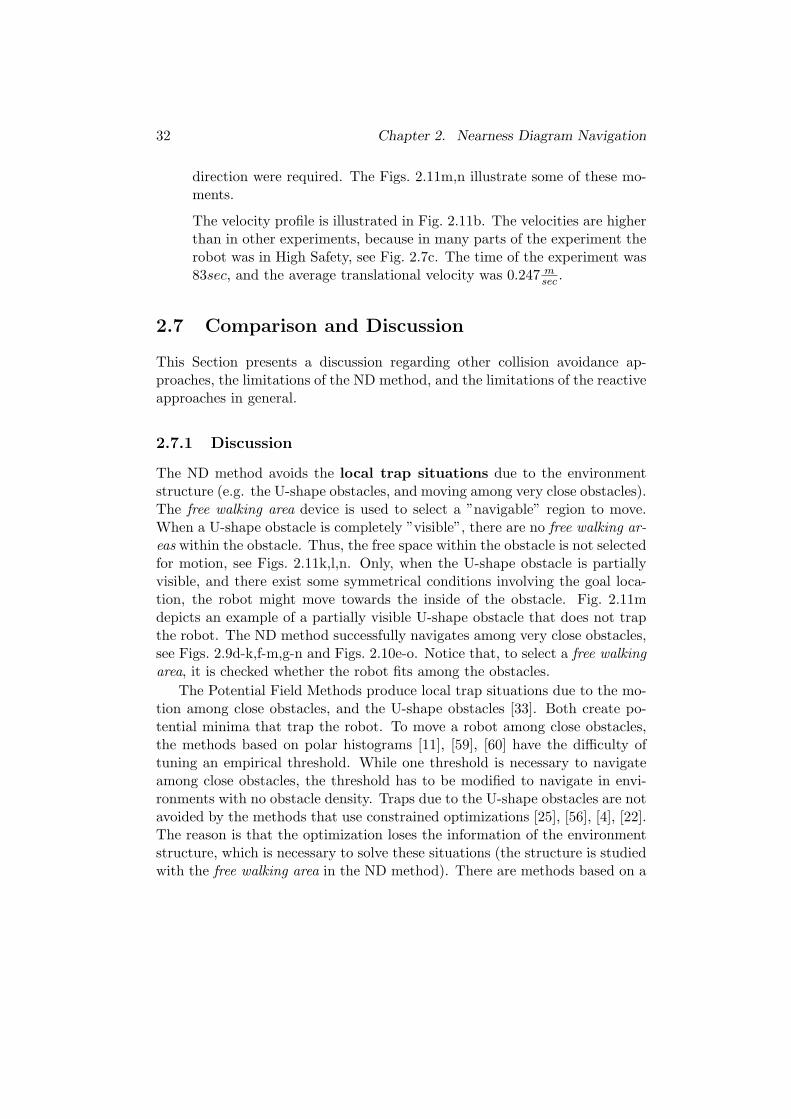
32 Chapter 2. Nearness Diagram Navigation
direction were required. The Figs. 2.11m,n illustrate some of these mo-ments.
The velocity profile is illustrated in Fig. 2.11b. The velocities are higherthan in other experiments, because in many parts of the experiment therobot was in High Safety, see Fig. 2.7c. The time of the experiment was83sec, and the average translational velocity was 0.247 m
sec .
2.7 Comparison and Discussion
This Section presents a discussion regarding other collision avoidance ap-proaches, the limitations of the ND method, and the limitations of the reactiveapproaches in general.
2.7.1 Discussion
The ND method avoids the local trap situations due to the environmentstructure (e.g. the U-shape obstacles, and moving among very close obstacles).The free walking area device is used to select a ”navigable” region to move.When a U-shape obstacle is completely ”visible”, there are no free walking ar-eas within the obstacle. Thus, the free space within the obstacle is not selectedfor motion, see Figs. 2.11k,l,n. Only, when the U-shape obstacle is partiallyvisible, and there exist some symmetrical conditions involving the goal loca-tion, the robot might move towards the inside of the obstacle. Fig. 2.11mdepicts an example of a partially visible U-shape obstacle that does not trapthe robot. The ND method successfully navigates among very close obstacles,see Figs. 2.9d-k,f-m,g-n and Figs. 2.10e-o. Notice that, to select a free walkingarea, it is checked whether the robot fits among the obstacles.
The Potential Field Methods produce local trap situations due to the mo-tion among close obstacles, and the U-shape obstacles [33]. Both create po-tential minima that trap the robot. To move a robot among close obstacles,the methods based on polar histograms [11], [59], [60] have the difficulty oftuning an empirical threshold. While one threshold is necessary to navigateamong close obstacles, the threshold has to be modified to navigate in envi-ronments with no obstacle density. Traps due to the U-shape obstacles are notavoided by the methods that use constrained optimizations [25], [56], [4], [22].The reason is that the optimization loses the information of the environmentstructure, which is necessary to solve these situations (the structure is studiedwith the free walking area in the ND method). There are methods based on a
2.7. Comparison and Discussion 33
given path that is deformed in real-time [54], [29], [14], [12]. When the pathlies within U-shape obstacles dynamically created a trap situation appears.
The ND method computes oscillation free motion when the robot movesamong very close obstacles. The Low Safety 2 action has been implemented tocomply with this requirement. The motion is computed from the two closestobstacles. See the complete robot path and the velocity profile in Figs. 2.9a,band Figs. 2.10a,b. The Potential Field Methods can produce oscillatory motionwhen moving among very close obstacles, or narrow corridors [33].
Motion directions far away from the goal direction are obtained with theND method (goal insensitivity). The reason is that the goal direction isdirectly used in only one of the five motion laws (in High Safety Goal in Region,where the robot is not in danger, and there is not an apparent navigationcomplexity). This property was determinant in many situations encounteredin the experiments, see Figs. 2.10h-q,i-r and Figs. 2.11e-l,g-n.
The reactive methods that make a physical analogy directly use the goallocation in the motion heuristic: potential field methods [30], [34], [58], [29],[9], [50], the perfume analogy [6], the fluid analogy [43]. These methods exhibithigh goal sensitivity. Thus, it is difficult to obtain directions far away fromthe goal location (in all the situations where they are required). The methodsthat solve the problem with a constrained optimization [25], [56], [4], [22] oneof the balance terms is the goal heading. Therefore these methods also exhibithigh goal sensitivity.
In the ND method action implementation, nothing prohibits the selectionof motion directions towards the obstacles. Thus, directions towardsobstacles are computed when required, see Figs. 2.9e-l,f-m,g-n, Figs. 2.10e-o,h-q,i-r, and Figs. 2.11k-c,l-e,m-f,n-g. Some methods explicitly prohibit theselection of motion towards the obstacles [59].
One difficulty found in most of the collision avoidance approaches is thetuning of the internal parameters. It is intricate to find the optimumvalues for a good behavior in all the collision avoidance situations. The NDmethod only has one parameter heuristically chosen (p parameter). This pa-rameter is only used in one of the five navigation laws, it is a multiplier of aphysical magnitude, and it is easy to find a value that does not determine thefinal method behavior.
The ND method uses five different situations and the associated actions tocompute the motion commands. Hysteresis was required to smooth transitionsbetween some situations.
Seen as a whole, the ND method is a robust reactive navigation method.This is mainly motivated by two facts:
34 Chapter 2. Nearness Diagram Navigation
1. The success of using a ”divide and conquer” strategy to decompose thereactive navigation problem in sub-problems (by different situations).Specific strategies for motion are then developed for any situation.
2. The free walking area is a device that endows the method with the guar-anty that: (1) it is possible to reach the goal, or (2) it is possible toreach the closest point to the goal, within the maximum reach of thelocal knowledge (sensory information).
2.7.2 Nearness Diagram Navigation Limitations
We think that the main limitation of the ND method is the method portabil-ity to different types of robots. The ND method does not take into accountthe so-called internal constraints of the robot: the shape, kinematic, and dy-namic constraints. The ND method is designed for a circular holonomic robotworking at low/medium velocities (' 0.5 m
sec).The methods of the related work take into account some of these con-
straints: the robot shape is considered in [30], [25], [4], and [22]. Some of themcompute motion commands that comply with the robot kinematics: [59], [25],[4], [22], and [56]. The robot dynamic constraints are taken into account in[25], [4], [22], and [56].
To deal with non-circular shapes is a difficult problem for the ND methodformulation. The ND method is formulated to apply over the Workspace,while the classical space used to represent the robot geometry is the Con-figuration space [39]. We have been working in this direction developing anunder-constrained solution for square and rectangular shapes, see Chapter 3.
Taking into account the kinematic constraints in the ND method formu-lation, we have developed the Ego-Kinematic Space. By means of a simpletransformation, the reactive navigation problem is carried out to a space wherethe robot is free of kinematic constraints. Standard reactive methods that donot take into account the robot kinematics (in particular the ND method) canbe applied in this space, and as a consequence, the solution complies with thekinematic constraints, see Chapter 4.
We have been working to introduce the robot dynamic constraints in theND method formulation. We have constructed a space where the dynamicconstraints are implicitly represented - the Ego-Dynamic Space. Standardreactive methods are used in this space. As a consequence, the reactive methodsolution complies with the dynamic constraints. By using this research, theND method velocity limits can be significantly increased, and still safety isguaranteed, see Chapter 5.
2.7. Comparison and Discussion 35
Another limitation of the reactive method design is that there is not a LowSafety situation whose action drives the robot towards the goal, when it isinside the security zone. This is a limitation of the reactive method design.However, the ND method does not have this limitation. The reason is thatthe robot can be in Low Safety 2 created by a virtual valley, see Fig. 2.6. Therobot would be driven towards the goal, irrespective of how close the goal isto the obstacle.
We have not addressed the sensor noise in the ND method implementation.We believe that external modules might process the sensory information inorder to deal with noisy sensors, see [10]. However, strategies such as increasingthe security distance according to the sensor uncertainty could be designed.
2.7.3 Improvements to all Reactive Approaches
The common limitation of all the reactive navigation methods analyzed in thisSection, including the ND method, is that they are purely local: global con-vergence to the goal location cannot be guaranteed. Recently, some researcheshave worked on introducing global information into the reactive methods toavoid the global trap situations. [60] uses a look ahead verification to analyzethe consequences of heading towards the candidate directions. The methodavoids the trap situations by running the algorithm a few steps in advanceof the algorithm execution. [14], [12] and Chapter 6 exploit the informationof the connectivity of the space using a navigation function. This providesthe reactive method with global information used to avoid the trap situations.Moreover, these two approaches take into account the so-called external con-straints: the nature of the environment. Both methods are adapted to workin highly dynamic scenarios.
2.7.4 Nearness Diagram Navigation Background
The ND method has been validated on the Diligent5robot at LAAS-CNRS(France). The reactive method has been successfully integrated as the low-level motion generator in the GenoM architecture [23], and the method is dailyused for demonstrations, see [1]. In the Robels system [51], the ND methodis one of the five sensory-motor functions used to move the robot. Two othersensory-motor functions are evolutions of the ND method, see Chapter 6.
With some modifications, the method is now working in other indoor/outdoor
5Diligent is a Nomadic XR4000 platform.
36 Chapter 2. Nearness Diagram Navigation
mobile platforms: Hilare, Hilare 26, and Lama7 at LAAS-CNRS (France);Otilio8 at University of Zaragoza (Spain), and r29 at Technical University ofLisbon (Portugal), see Chapter 3. Currently, the method is being implementedon Dalay10 at LAAS-CNRS (France).
2.8 Conclusions
This Chapter presents the design of a reactive navigation method. It has beendesigned using the situated-activity paradigm of behavioral design. The designof the method is the basis to implement reactive navigation methods. Theadvantage is that the paradigm used in the design employs a “divide and con-quer” strategy to reduce the difficulty of the problem. As a consequence, thereactive navigation methods implemented, following the presented guidelines,might be able to successfully navigate in more troublesome scenarios thanother methods do.
At the current moment, the method design has been used to implementsome reactive navigation methods that adapt to their collision avoidance con-text. For example the Free Zone Method [41], [42] for soccer player robots.We have used the method design to implement the ND method. The maincontribution of this method is that it robustly achieves navigation in verydense, cluttered, and complex scenarios. These environments are a challengefor many existing methods.
The method can be extended to three dimensions. The information col-lected to define the situations, and the geometry-based implementation of theactions, both can easily be redefined to the third dimension. This will allowfor generating reactive collision avoidance for free-flying objects working inthree-dimensional workspaces.
6Hilare and Hilare2 are indoor rectangular differential-driven robots. The main sensorsused were two 2D planar laser.
7Lama is a rectangular outdoor robot that can work in differential-driven mode. Thesensor used was a pair B/W cameras.
8Otilio is square and differential-driven indoor robot. The sensor used was a 3D laser.9r2 is a circular and differential-driven indoor robot. The sensor used was a ring of
ultrasounds sensors.10Dalay is a rectangular and differential-driven outdoor robot. The sensor being used is a
2D laser.
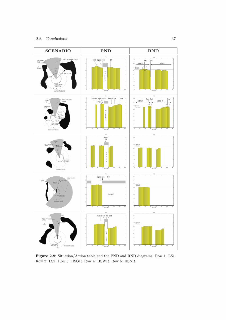
2.8. Conclusions 37
SCENARIO PND RND
SECURITY ZONE
SECURITYDISTANCE
θ
GAP
FREE WALKING AREA
Sp
S SOLUTION
GOAL X
Sml
Srd
CLOSEST
0 20 40 60 80 100 120 1400
0.5
1
1.5
2
2.5
3
3.5
4
SECTORS
PND
θS
VALLEY
SrdSgoalSml
0 20 40 60 80 100 120 1400
0.5
1
1.5
2
2.5
3
3.5
4
SECTORS
RND
SIDE 1 SIDE 2
SecurityNearness
SrdSml
FREE WALKING
C
SECURITY ZONE
GOAL X
AREA
SOLUTIONθS
Smed1
SECURITYDISTANCE
Smed2
GAP
Sml
Smr
CLOSEST
Srd
0 20 40 60 80 100 120 1400
0.5
1
1.5
2
2.5
3
3.5
4
SECTORS
PND
Sθ
VALLEY
Smed2 Smed1Sgoal Srd
Sml
Smr
0 20 40 60 80 100 120 1400
0.5
1
1.5
2
2.5
3
3.5
4
SECTORS
RND
SrdSIDE 1 SIDE 2
SecurityNearness
SmrSml
SECURITY ZONE
GOAL X
AREAFREE WALKING
SθSOLUTION
DISTANCESECURITY
0 20 40 60 80 100 120 1400
0.5
1
1.5
2
2.5
3
3.5
4
SECTORS
PND
θSSgoal
VALLEY
0 20 40 60 80 100 120 1400
0.5
1
1.5
2
2.5
3
3.5
4
SECTORS
RND
NearnessSecurity
X θGOAL
SECURITY ZONE
S SOLUTION
Smax/2
FREE WALKINGAREA
Srd
SECURITYDISTANCE
0 20 40 60 80 100 120 1400
0.5
1
1.5
2
2.5
3
3.5
4
SECTORS
PND
Sgoal SθSrd
VALLEY
0 20 40 60 80 100 120 1400
0.5
1
1.5
2
2.5
3
3.5
4
SECTORS
RND
NearnessSecurity
X θ
FREE WALKINGAREA
GOAL
S SOLUTION
SECURITY ZONESECURITY
DISTANCE
SodSrd
0 20 40 60 80 100 120 1400
0.5
1
1.5
2
2.5
3
3.5
4
SECTORS
PND
SθSgoal Srd Sod
VALLEY
0 20 40 60 80 100 120 1400
0.5
1
1.5
2
2.5
3
3.5
4
SECTORS
RND
NearnessSecurity
Figure 2.8: Situation/Action table and the PND and RND diagrams. Row 1: LS1.Row 2: LS2. Row 3: HSGR. Row 4: HSWR. Row 5: HSNR.
38 Chapter 2. Nearness Diagram Navigation
Snapshot 1
Snapshot 2
Snapshot 3
Snapshot 4
Snapshot 5
Snapshot 6
Snapshot 7
Snapshot 8
xGOAL
1 meter
0 10 20 30 40 50−0.5
0
0.5Velocities
Time (sec)
X V
eloc
ity (
m/s
ec)
0 10 20 30 40 50−0.5
0
0.5
Time (sec)
Y V
eloc
ity (
m/s
ec)
0 10 20 30 40 50
−1
0
1
Time (sec)
Rot
atio
nal V
eloc
ity (
rad/
sec)
(a) (b)
(c) (d) (e) (f)
GOAL
(g) (h) (i) (j)
ROBOT
ND SOLUTION
LASER POINTS
x GOAL
ROBOT
LASER POINTS
ND SOLUTION
x GOAL
(k) (l) (m) (n)
Figure 2.9: Experiment 1.
2.8. Conclusions 39
Snapshot 1
Snapshot 2
GOAL
Snapshot 7
Snapshot 6
Snapshot 5
BLOCKEDPASSAGE
Snapshot 4
Snapshot 8 X
1 meter
Snapshot 3
0 50 100 150 200−0.5
0
0.5Velocities
Time (sec)
X V
eloc
ity (
m/s
ec)
0 50 100 150 200−0.5
0
0.5
Time (sec)
Y V
eloc
ity (
m/s
ec)
0 50 100 150 200
−1
0
1
Time (sec)
Rot
atio
nal V
eloc
ity (
rad/
sec)
(a) (b)
U−SHAPE
OBSTACLE
(c) (d) (e) (f)
(g) (h) (i) (j)
XGOAL
(k) (l) (m) (n)
GOAL PASSAGECLOSED
GOALDIRECTION GOAL
DIRECTION
(o) (p) (q) (r)
Figure 2.10: Experiment 2.
40 Chapter 2. Nearness Diagram Navigation
Snapshot 1
Snapshot 2
Snapshot 3
Snapshot 5
Snapshot 6
Snapshot 8
xGOAL
Snapshot 4
Snapshot 7
U−SHAPE OBSTACLES
1 meter
0 10 20 30 40 50 60 70−0.5
0
0.5Velocities
Time (sec)
X V
eloc
ity (
m/s
ec)
0 10 20 30 40 50 60 70−0.5
0
0.5
Time (sec)
Y V
eloc
ity (
m/s
ec)
0 10 20 30 40 50 60 70
−1
0
1
Time (sec)
Rot
atio
nal V
eloc
ity (
rad/
sec)
(a) (b)
U−SHAPE
OBSTACLES
GOAL
(c) (d) (e) (f)
U−SHAPE
OBSTACLES
GOAL
XGOAL
(g) (h) (i) (j)
GOAL
DIRECTION
U−SHAPE
OBSTACLE
GOAL
DIRECTION
U−SHAPE
OBSTACLE
U−SHAPE
OBSTACLE
GOAL
DIRECTIONDIRECTION
GOAL
OBSTACLE
U−SHAPE
(k) (l) (m) (n)
Figure 2.11: Experiment 3.
Chapter 3
Under-constrainedSensor-Based MotionPlanning
3.1 Introduction
In typical mobile robotic missions, the indoor/outdoor environment is un-known and non-predictable (e.g. offices, museums, planetary surfaces). Fromthe navigation point of view, the different nature of these scenarios imposesa wide range of difficulties: they are unstructured, dense, cluttered, etc. Inaddition, the robots designed usually exhibit different shapes, kinematics, anddynamics. In these scenarios, the robot shape, kinematics, and dynamics playan important role, since they constrain the possible robot motions.
This Chapter presents an under-constrained solution to address the shape,kinematics, and dynamics in the reactive navigation layer. This solution isused to extend the Nearness Diagram Navigation (Chapter 2) to computecommands that comply with these constraints.
The solution proposed is under-constrained since the shape, kinematics,and dynamics are taken into account after the reactive method usage. Thus,while the motion commands comply with the constraints, they are not usedfrom the beginning in the motion commands computation.
The advantage of the framework is the integration methodology, the easyportability among platforms, and the navigation results. The method suc-cessfully achieves navigation, with different robots and sensors, in very dense,complex, and cluttered scenarios. To demonstrate the easy portability among
41
42 Chapter 3. Under-constrained Sensor-Based Motion Planning
different platforms, the method has been tested on four indoor robots and onone outdoor robot at three different laboratories.
This research was previously presented in [45].The paper is distributed as follows. Section 3.2 discusses related work. Sec-
tion 3.3 introduces the framework and Section 3.4 presents the experimentalresults. Finally, in Section 3.5 the conclusions are drawn.
3.2 Related Work
To design the safe motion generation task, there are at least three issues toaddress: the navigation method, the robot kinematics and dynamics, and therobot shape.
The navigation technique used is a reactive navigation method [30], [11],[59], [25], [44], [54], among others. Based on a perception-action process, thesemethods compute collision-free motion commands in a goal-directed fashion.The main advantage is that these methods require a low computational load.This provides the system with the possibility of a high-rate environmentalfeedback. The drawbacks of these approaches are that they produce sub-optimal solutions, and they cannot guarantee the reach of the goal location.A deeper discussion about these methods is presented in Chapter 2.
Currently, most of the robots designed exhibit kinematic and dynamicconstraints. For these robots, the navigation method has to take into accountthese constraints. Otherwise, the robot cannot execute the motion computedby the reactive navigation method [30], [11], [44], [54]. This issue will bediscussed in detail in Chapters 4, and 5.
The robot shape is a difficult problem in reactive navigation. Classically,the robot shape is taken into account by carrying out the problem to the Con-figuration space [35]. In this space, a point represents the robot. To map theobstacles into the Configuration space is a time-consuming task not comply-ing with the real-time requirement. Some reactive navigation methods avoidthe Configuration space computation, by approximating the robot by circularshapes. Thus, the collision checking can be carried out in the Workspace [11],[44], [54]. If these methods are used over non-circular bases, the robot shapeneeds to be approximated, under-constraining the method solution. This issuewill be discussed in detail in Chapter 4.
This Chapter addresses the robot motion in very dense, complex, and clut-tered scenarios. The robot shape, kinematics, and dynamics are determinantin these scenarios, and thus, they cannot be neglected. The Nearness DiagramNavigation method is a reactive navigation method that successfully navigates
3.3. The Framework 43
in those scenarios. However, the Nearness Diagram Navigation method doesnot consider the robot shape, kinematics, and dynamics. For this reason, thisChapter addresses the extension of the Nearness Diagram Navigation methodto take into account the robot shape, kinematics, and dynamics.
3.3 The Framework
The goal of this Section is to understand the solution proposed to extend theNearness Diagram Navigation method to address the shape, kinematics, anddynamics.
The solution is based on breaking down the motion computation processinto three sub-problems related to: (1) collision avoidance, (2) the robot kine-matic and dynamic constraints, and (3) the robot shape:
1. The reactive collision avoidance approach - Nearness Diagram Naviga-tion - is used to calculate the most promising motion direction and thedesired velocity. The assumption is a circular robot free of motion con-straints.
2. The Motion Generator uses the information provided by the NearnessDiagram Navigation method to compute a motion command that com-plies with the kinematic and dynamic constraints.
3. For non-circular robots, the Shape Corrector modifies the pre-computedmotion command to take into account the robot shape.
Fig. 3.1 illustrates the complete process. Seen as a whole, this frameworkcomputes collision-free motion commands to drive a mobile platform towards agiven goal location. The motion commands comply with the robot kinematicsand dynamics, and the robot shape is considered.
The three modules are next analyzed.
3.3.1 Nearness Diagram Navigation
The Nearness Diagram Navigation (ND) method is described in detail in Chap-ter 2. However, a brief description of the method is next presented. The NDmethod is based on the situated-activity methodology of design [3]. First, aset of five situations that fully describe the relative state of the robot, ob-stacle distribution, and goal location are defined. Subsequently, one action isdesigned for each situation. In real-time, the sensory information is used to
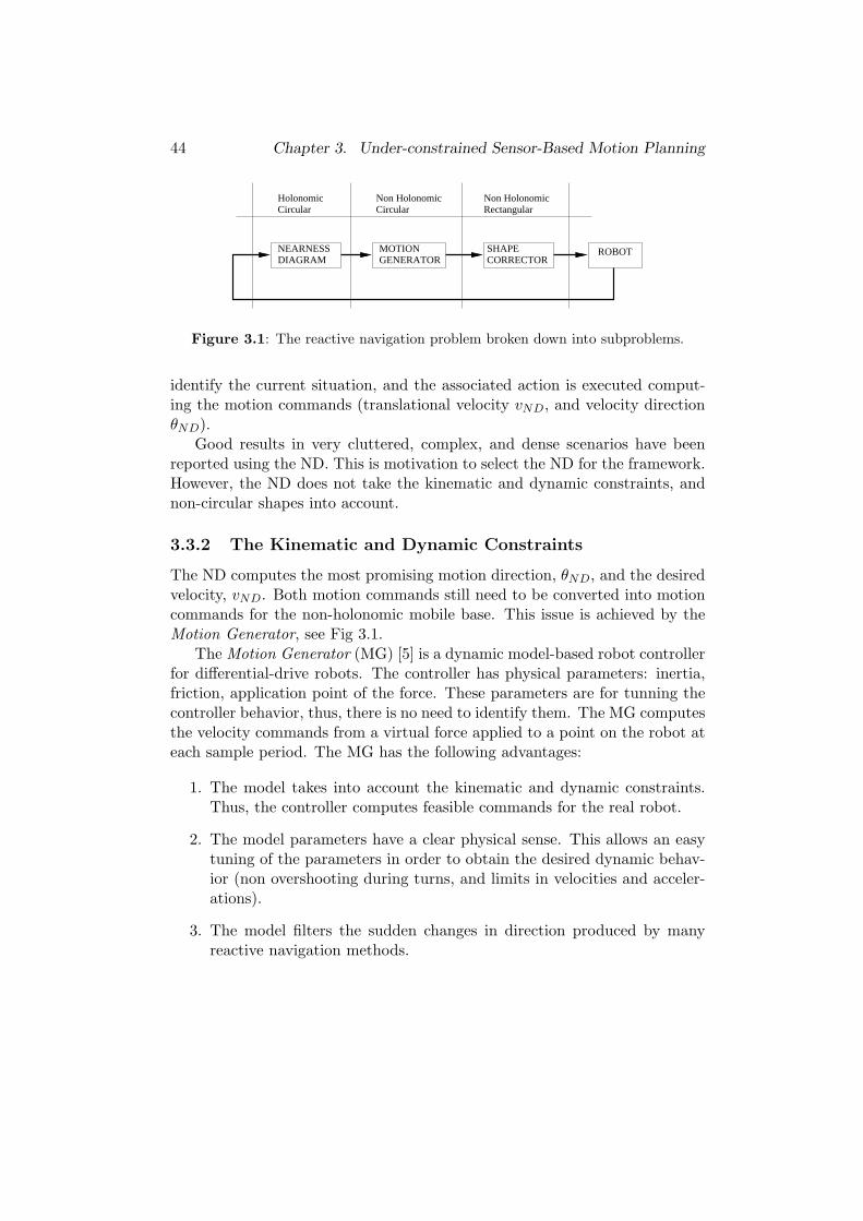
44 Chapter 3. Under-constrained Sensor-Based Motion Planning
NEARNESSDIAGRAM
MOTIONGENERATOR
SHAPECORRECTOR
HolonomicCircular
Non HolonomicCircular
Non HolonomicRectangular
ROBOT
Figure 3.1: The reactive navigation problem broken down into subproblems.
identify the current situation, and the associated action is executed comput-ing the motion commands (translational velocity vND, and velocity directionθND).
Good results in very cluttered, complex, and dense scenarios have beenreported using the ND. This is motivation to select the ND for the framework.However, the ND does not take the kinematic and dynamic constraints, andnon-circular shapes into account.
3.3.2 The Kinematic and Dynamic Constraints
The ND computes the most promising motion direction, θND, and the desiredvelocity, vND. Both motion commands still need to be converted into motioncommands for the non-holonomic mobile base. This issue is achieved by theMotion Generator, see Fig 3.1.
The Motion Generator (MG) [5] is a dynamic model-based robot controllerfor differential-drive robots. The controller has physical parameters: inertia,friction, application point of the force. These parameters are for tunning thecontroller behavior, thus, there is no need to identify them. The MG computesthe velocity commands from a virtual force applied to a point on the robot ateach sample period. The MG has the following advantages:
1. The model takes into account the kinematic and dynamic constraints.Thus, the controller computes feasible commands for the real robot.
2. The model parameters have a clear physical sense. This allows an easytuning of the parameters in order to obtain the desired dynamic behav-ior (non overshooting during turns, and limits in velocities and acceler-ations).
3. The model filters the sudden changes in direction produced by manyreactive navigation methods.
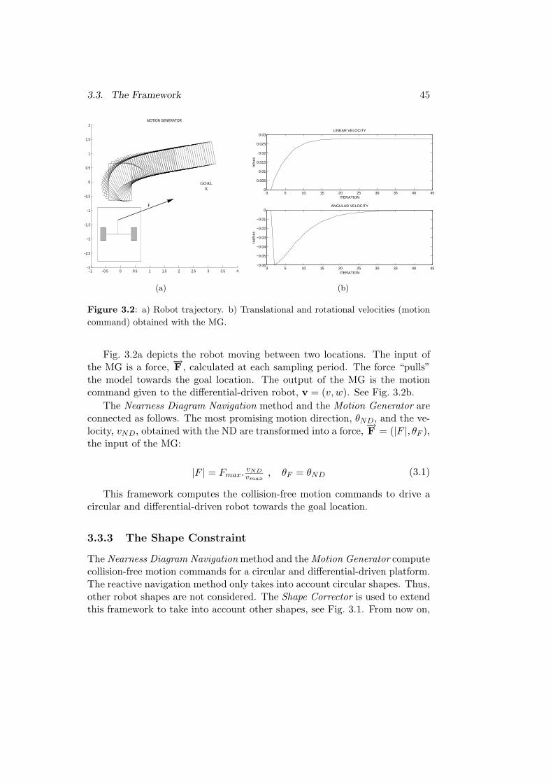
3.3. The Framework 45
−1 −0.5 0 0.5 1 1.5 2 2.5 3 3.5 4−3
−2.5
−2
−1.5
−1
−0.5
0
0.5
1
1.5
2MOTION GENERATOR
XGOAL
F
0 5 10 15 20 25 30 35 40 450
0.005
0.01
0.015
0.02
0.025
0.03LINEAR VELOCITY
ITERATION
m/s
ec
0 5 10 15 20 25 30 35 40 45−0.06
−0.05
−0.04
−0.03
−0.02
−0.01
0ANGULAR VELOCITY
ITERATION
rad/
sec
(a) (b)
Figure 3.2: a) Robot trajectory. b) Translational and rotational velocities (motioncommand) obtained with the MG.
Fig. 3.2a depicts the robot moving between two locations. The input ofthe MG is a force, −→F , calculated at each sampling period. The force “pulls”the model towards the goal location. The output of the MG is the motioncommand given to the differential-driven robot, v = (v, w). See Fig. 3.2b.
The Nearness Diagram Navigation method and the Motion Generator areconnected as follows. The most promising motion direction, θND, and the ve-locity, vND, obtained with the ND are transformed into a force, −→F = (|F |, θF ),the input of the MG:
|F | = Fmax. vNDvmax
, θF = θND (3.1)
This framework computes the collision-free motion commands to drive acircular and differential-driven robot towards the goal location.
3.3.3 The Shape Constraint
The Nearness Diagram Navigation method and the Motion Generator computecollision-free motion commands for a circular and differential-driven platform.The reactive navigation method only takes into account circular shapes. Thus,other robot shapes are not considered. The Shape Corrector is used to extendthis framework to take into account other shapes, see Fig. 3.1. From now on,
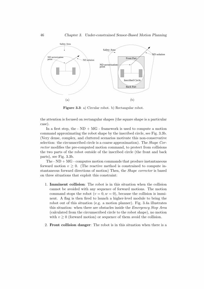
46 Chapter 3. Under-constrained Sensor-Based Motion Planning
Safety Area
ND sectorizationpoint ND solution
Safety Area
ND sectorizationpoint
ND solution
Front Part
Back Part
Inscribed Circle
(a) (b)
Figure 3.3: a) Circular robot. b) Rectangular robot.
the attention is focused on rectangular shapes (the square shape is a particularcase).
In a first step, the - ND + MG - framework is used to compute a motioncommand approximating the robot shape by the inscribed circle, see Fig. 3.3b.(Very dense, complex, and cluttered scenarios motivate this non-conservativeselection: the circumscribed circle is a coarse approximation). The Shape Cor-rector modifies the pre-computed motion command, to protect from collisionsthe two parts of the robot outside of the inscribed circle (the front and backparts), see Fig. 3.3b.
The - ND + MG - computes motion commands that produce instantaneousforward motion v ≥ 0. (The reactive method is constrained to compute in-stantaneous forward directions of motion) Then, the Shape corrector is basedon three situations that exploit this constraint:
1. Imminent collision: The robot is in this situation when the collisioncannot be avoided with any sequence of forward motions. The motioncommand stops the robot (v = 0, w = 0), because the collision is immi-nent. A flag is then fired to launch a higher-level module to bring therobot out of this situation (e.g. a motion planner). Fig. 3.4a illustratesthis situation: when there are obstacles inside the Emergency Stop Area(calculated from the circumscribed circle to the robot shape), no motionwith v ≥ 0 (forward motion) or sequence of them avoid the collision.
2. Front collision danger: The robot is in this situation when there is a
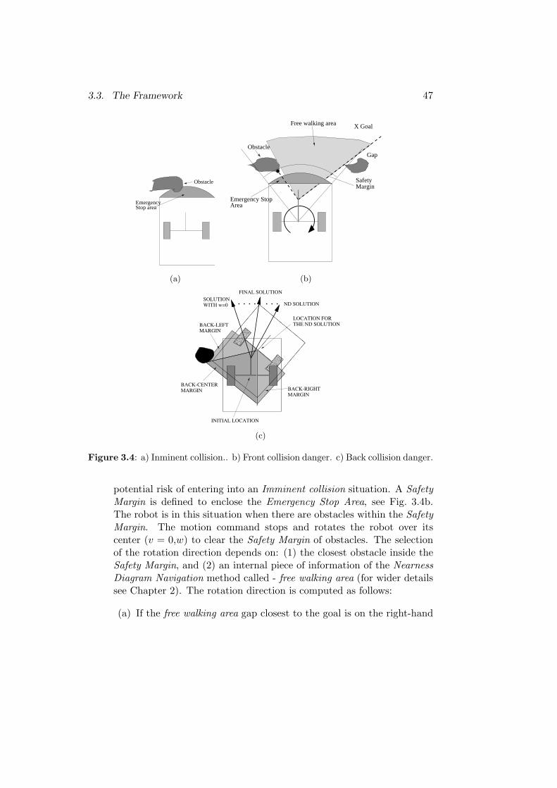
3.3. The Framework 47
EmergencyStop area
Obstacle SafetyMargin
GapObstacle
Emergency StopArea
X GoalFree walking area
(a) (b)
BACK-LEFT
MARGIN
BACK-RIGHT
MARGIN
BACK-CENTER
MARGIN
WITH w=0
SOLUTION
LOCATION FOR
THE ND SOLUTION
INITIAL LOCATION
FINAL SOLUTION
ND SOLUTION. . .. . . .
(c)
Figure 3.4: a) Inminent collision.. b) Front collision danger. c) Back collision danger.
potential risk of entering into an Imminent collision situation. A SafetyMargin is defined to enclose the Emergency Stop Area, see Fig. 3.4b.The robot is in this situation when there are obstacles within the SafetyMargin. The motion command stops and rotates the robot over itscenter (v = 0,w) to clear the Safety Margin of obstacles. The selectionof the rotation direction depends on: (1) the closest obstacle inside theSafety Margin, and (2) an internal piece of information of the NearnessDiagram Navigation method called - free walking area (for wider detailssee Chapter 2). The rotation direction is computed as follows:
(a) If the free walking area gap closest to the goal is on the right-hand
48 Chapter 3. Under-constrained Sensor-Based Motion Planning
of the direction of the closest obstacle inside the Safety Margin,then the robot rotates towards the right. If not,
(b) The robot rotates towards the left.
The result of this strategy clears the Safety Margin of obstacles, implic-itly avoiding the Imminent collision situation. Fig. 3.4b illustrates anexample of this situation, in which the robot stops and rotates towardsthe right.
3. Back collision danger: The robot is in this situation when the pre-computed motion command produces a collision with the back part ofthe robot. To detect this situation, the trajectory that would be obtainedunder the execution of the pre-computed motion command is analyticallycalculated (following [25]). Then, the robot motion is simulated over thetrajectory checking collisions, to validate the motion command. Theback part of the robot is enlarged for safety reasons. The back of therobot is divided into three parts Back-Left, Back-Right and Back-CenterSafety Margins, see Fig. 3.4c. Then, three cases distinguished:
• A collision is detected with the Back-Left Margin. The angle between theND solution and the direction that would produce w = 0, is discretized insub-directions. The MG computes a new motion command by using oneof those sub-directions. The new motion command is tested for collisionsover the trajectory. This procedure is repeated until a collision-freemotion command is found. Fig. 3.4c illustrates an example where thepre-computed motion command produces a collision with the Back-LeftMargin. Some intermediate directions are tested, until a collision-freecommand is found.
• A collision is detected with the Back-Right Margin. The above procedureis repeated but towards the right-hand direction.
• A collision is detected with Back-Center Margin, or simultaneously withBack-Left and Back-Right Margins. The motion command is a forwardmotion without rotation (v ≥ 0,w = 0).
This framework computes the collision-free motion commands to drive arectangular and differential-driven robot towards the goal location.
3.4. Experimental Results 49
3.4 Experimental Results
This Section validates experimentally the proposed research. This frameworkhas been tested on four indoor robots and on one outdoor robot. The maincharacteristics of the robots are: (1) they are differential-driven robots, withthe exception of the outdoor robot that can be set to work in differential-driven mode. (2) The robots have circular, square, and rectangular shapes.(3) The on-board sensors are ultrasounds, 2D and 3D laser rangefinders, anda stereo pair of cameras.
To adapt the framework to each robot, the main adjustments were: (1)an special safety area (for each robot shape) was designed for the NearnessDiagram Navigation method, see Fig. 3.3a and Fig. 3.3b. (2) The MotionGenerator parameters were tuned to have the desired dynamic behavior com-patible with each platform constraints (due to the different motion capabilitiesof each robot). (3) Only some geometric parameters were changed in the ShapeCorrector.
In all the experiments the environment was completely unknown, and onlythe goal location was given in advance to the robot. The environments wereunstructured (random shaped obstacles). Nevertheless, the environment couldbe dynamic and non-predictable. Under all these circumstances it is widelyjustified the use of reactive navigation algorithms to move the robot.
The experiments reported have a common objective: To show that thisframework is able to safely drive a kinematic and dynamic constrained mobileplatform in very dense, complex and cluttered scenarios. This is the type ofscenarios where other approaches are susceptible to failure for the followingreasons: (1) the reactive method itself, (2) approximations in the motionexecuted, and (3) approximations in the robot shape.
3.4.1 Circular robots
For circular robots the Nearness Diagram Navigation + Motion Generatorframework is used.
Nomadic Scout
This framework has been implemented in a Nomadic Scout at the InstitutoSuperior Tecnico de Lisboa, Portugal, see Appendix E.0.7.
Fig. 3.3a illustrates the robot model and the point used to apply the ND.The sampling time was T = 0.25sec and the maximum speed v = 0.3 m
sec .
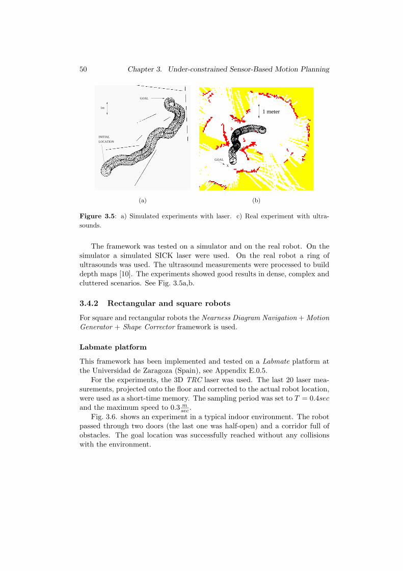
50 Chapter 3. Under-constrained Sensor-Based Motion Planning
INITIAL
LOCATION
1m
XGOAL
GOAL
X
1 meter
(a) (b)
Figure 3.5: a) Simulated experiments with laser. c) Real experiment with ultra-sounds.
The framework was tested on a simulator and on the real robot. On thesimulator a simulated SICK laser were used. On the real robot a ring ofultrasounds was used. The ultrasound measurements were processed to builddepth maps [10]. The experiments showed good results in dense, complex andcluttered scenarios. See Fig. 3.5a,b.
3.4.2 Rectangular and square robots
For square and rectangular robots the Nearness Diagram Navigation + MotionGenerator + Shape Corrector framework is used.
Labmate platform
This framework has been implemented and tested on a Labmate platform atthe Universidad de Zaragoza (Spain), see Appendix E.0.5.
For the experiments, the 3D TRC laser was used. The last 20 laser mea-surements, projected onto the floor and corrected to the actual robot location,were used as a short-time memory. The sampling period was set to T = 0.4secand the maximum speed to 0.3 m
sec .Fig. 3.6. shows an experiment in a typical indoor environment. The robot
passed through two doors (the last one was half-open) and a corridor full ofobstacles. The goal location was successfully reached without any collisionswith the environment.
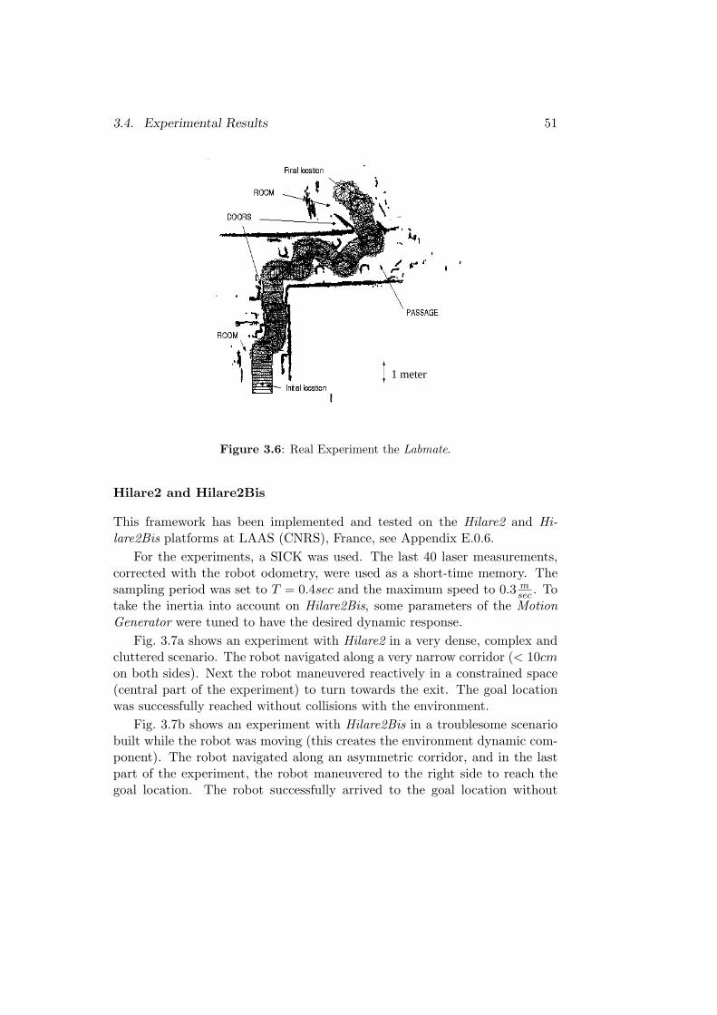
3.4. Experimental Results 51
1 meter
Figure 3.6: Real Experiment the Labmate.
Hilare2 and Hilare2Bis
This framework has been implemented and tested on the Hilare2 and Hi-lare2Bis platforms at LAAS (CNRS), France, see Appendix E.0.6.
For the experiments, a SICK was used. The last 40 laser measurements,corrected with the robot odometry, were used as a short-time memory. Thesampling period was set to T = 0.4sec and the maximum speed to 0.3 m
sec . Totake the inertia into account on Hilare2Bis, some parameters of the MotionGenerator were tuned to have the desired dynamic response.
Fig. 3.7a shows an experiment with Hilare2 in a very dense, complex andcluttered scenario. The robot navigated along a very narrow corridor (< 10cmon both sides). Next the robot maneuvered reactively in a constrained space(central part of the experiment) to turn towards the exit. The goal locationwas successfully reached without collisions with the environment.
Fig. 3.7b shows an experiment with Hilare2Bis in a troublesome scenariobuilt while the robot was moving (this creates the environment dynamic com-ponent). The robot navigated along an asymmetric corridor, and in the lastpart of the experiment, the robot maneuvered to the right side to reach thegoal location. The robot successfully arrived to the goal location without
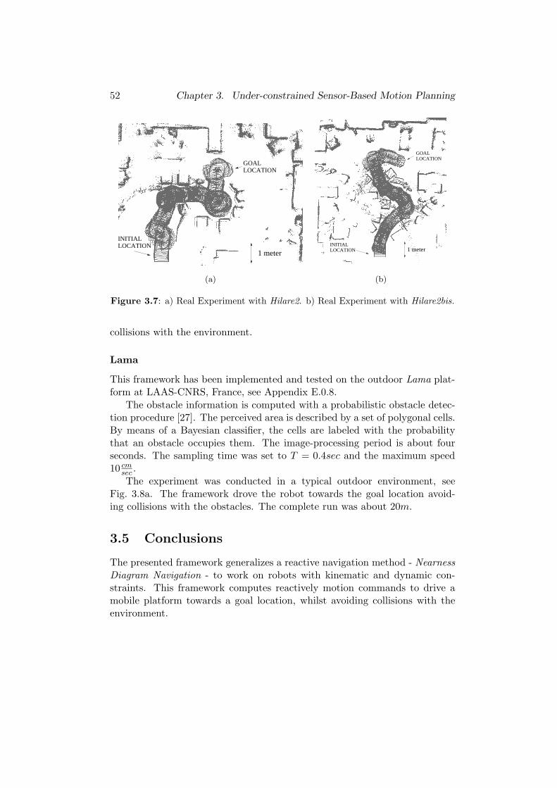
52 Chapter 3. Under-constrained Sensor-Based Motion Planning
GOAL LOCATION
INITIAL LOCATION
1 meter
GOALLOCATION
INITIAL LOCATION 1 meter
(a) (b)
Figure 3.7: a) Real Experiment with Hilare2. b) Real Experiment with Hilare2bis.
collisions with the environment.
Lama
This framework has been implemented and tested on the outdoor Lama plat-form at LAAS-CNRS, France, see Appendix E.0.8.
The obstacle information is computed with a probabilistic obstacle detec-tion procedure [27]. The perceived area is described by a set of polygonal cells.By means of a Bayesian classifier, the cells are labeled with the probabilitythat an obstacle occupies them. The image-processing period is about fourseconds. The sampling time was set to T = 0.4sec and the maximum speed10 cm
sec .The experiment was conducted in a typical outdoor environment, see
Fig. 3.8a. The framework drove the robot towards the goal location avoid-ing collisions with the obstacles. The complete run was about 20m.
3.5 Conclusions
The presented framework generalizes a reactive navigation method - NearnessDiagram Navigation - to work on robots with kinematic and dynamic con-straints. This framework computes reactively motion commands to drive amobile platform towards a goal location, whilst avoiding collisions with theenvironment.
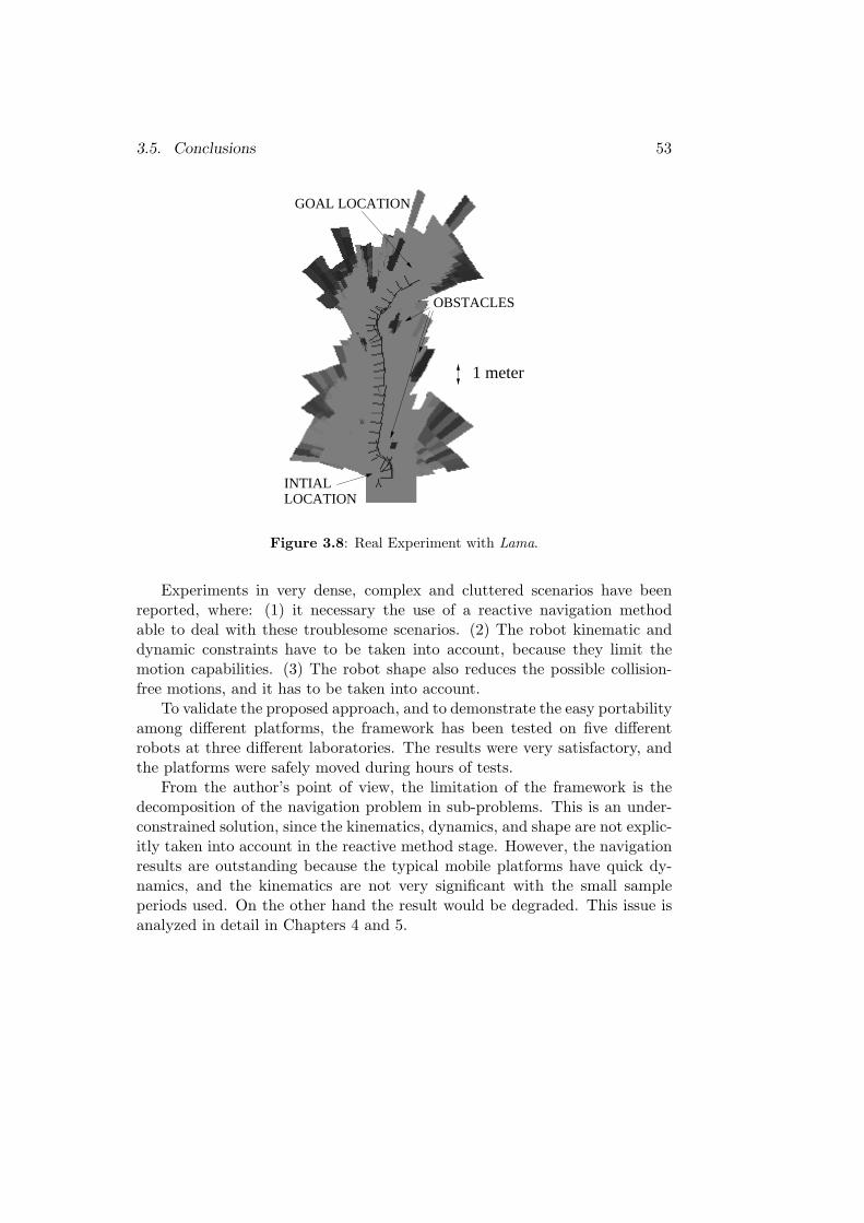
3.5. Conclusions 53
INTIAL LOCATION
GOAL LOCATION
OBSTACLES
1 meter
Figure 3.8: Real Experiment with Lama.
Experiments in very dense, complex and cluttered scenarios have beenreported, where: (1) it necessary the use of a reactive navigation methodable to deal with these troublesome scenarios. (2) The robot kinematic anddynamic constraints have to be taken into account, because they limit themotion capabilities. (3) The robot shape also reduces the possible collision-free motions, and it has to be taken into account.
To validate the proposed approach, and to demonstrate the easy portabilityamong different platforms, the framework has been tested on five differentrobots at three different laboratories. The results were very satisfactory, andthe platforms were safely moved during hours of tests.
From the author’s point of view, the limitation of the framework is thedecomposition of the navigation problem in sub-problems. This is an under-constrained solution, since the kinematics, dynamics, and shape are not explic-itly taken into account in the reactive method stage. However, the navigationresults are outstanding because the typical mobile platforms have quick dy-namics, and the kinematics are not very significant with the small sampleperiods used. On the other hand the result would be degraded. This issue isanalyzed in detail in Chapters 4 and 5.

54 Chapter 3. Under-constrained Sensor-Based Motion Planning
Chapter 4
Sensor-Based MotionPlanning with KinematicConstraints
4.1 Introduction
Even though many robots exhibit kinematic constraints, most sensor-basednavigation methods do not take these constraints into account. This is a hardlimitation when using a navigation method. The robot can only approximatelyexecute the motion computed: safety cannot be longer guaranteed. In othercases, some sensor-based algorithms have been extended to address the motionconstraints. However, with this approach, the reactive navigation method isusually re-designed from scratch to address the constraints. And a new re-design might be necessary to incorporate the constraints of another robot.
There is a lot of literature that proposes particular solutions to addressthe motion constraints in the sensor-based motion planning field. But littleattention has been paid to look for much wider solutions.
This Chapter presents a novel idea to take into account the kinematicconstraints: to introduce them in the space. The proposal is to use the kine-matics to construct a novel spatial representation, the Ego-Kinematic Space.The kinematic constraints are embedded in the space, so the robot in this spacemoves as a ”free-flying” object. Then, standard sensor-based algorithms thatdo not take into account the kinematic constraints can be used in this space.As a consequence, the algorithms comply with the kinematics without address-ing it directly. By using this approach, it is straightforward to apply existing
55
56 Chapter 4. Sensor-Based Motion Planning with Kinematic Constraints
reactive navigation algorithms to non-holonomic robots. An ample solution, toaddress the motion constraints in the sensor-based motion planning discipline,is presented.
Another problem overcame in this Chapter is the space dimensionality.The Configuration space for non-holonomic robots such as differential-drivenrobots, tri-cycle robots, and car-like robots is three-dimensional IR2 × S1.In the sensor-based motion planning context, the computations required todeal with three dimensions are a limitation: these algorithms have to workin real-time. The necessity of using only a subspace of the Configurationspace with the same structure of the Workspace, IR2, is demonstrated. Assuch, the dimension of the Configuration space is reduced by one within thecontext of sensor-based motion planning. This will alleviate significantly thecomputation time of future sensor-based algorithms that make use of thisresult. In particular, the research presented in this Chapter.
The main advantage of this framework is that it can be utilized by relatedwork. Many sensor-based algorithms, that do not take into account the kine-matic constraints, can be used in the proposed spatial representation, withoutfurther concern about the kinematic constraints. Experimental results involv-ing a non-holonomic robot are shown to validate the framework. Two methodswere used for navigation (Nearness Diagram Navigation, Chapter 2, and thePotential Field Method [30]). They both originally do not address kinematics.By using the framework both methods were successfully used to safely drivethe constrained platform among locations.
This research was previously presented in [47].
The Chapter is organized as follows: In Section 4.2 a general backgroundfor the rest of the Chapter is introduced. Section 4.3 discusses the Configura-tion space dimensionality. The Ego-Kinematic Space is addressed in Section4.4. Finally, Section 4.5 shows the experimental results and Section 4.6 drawsthe conclusions.
4.2 Background and Preliminaries
This Section reviews some concepts used in the remaining part of the Chapter.Firstly, the robot kinematics covered by the analysis is presented. Secondly,the sensor-based motion planning techniques are discussed. Finally, the ad-missible paths that arise from the robot kinematic model are examined.
4.2. Background and Preliminaries 57
4.2.1 Robot Kinematics
Robots moving on a flat surface with the classical hypothesis “rolling withoutslipping” are addressed. The Workspace, W, and the Configuration space, C,are IR2 and IR2 × S1 respectively. A robot configuration is represented by itslocation and the orientation q = (x, y, θ). The attention is focused on robotswhose motion is constrained by:
−xsinθ + ycosθ = 0 (4.1)
Equation 4.1 is a non-holonomic equality constraint. The effect is toreduce by one the dimension of the space of differential motions at any givenconfiguration [7]. Hence, a motion command of the robot can be described bytwo motion parameters only.
The kinematic model of the two-driving wheels and the car-like mobilerobots is next described. These robots are representative examples of mobileplatforms that verify the constraint of Equation (4.1), see Fig. 4.1. A deeperdescription of both models is found in [36].
The kinematic model of both, the two-driving wheels and car-like robots,can be expressed by the following equation (the difference is a change of vari-able12), as detailed in [36]:
x
y
θ
=
cosθ
sinθ
0
v+
0
0
1
w (4.2)
where v and w denote the linear and angular velocities.The main difference between these two platforms is that the car-like robot
has a mechanical constraint. This imposes a maximum curvature γmax (orminimum turning radius rmin = γ−1
max) of the path executed by the robot.There are other robots (e.g. tri-cycle robots) whose kinematic models can alsobe expressed by Equation (4.2), and verify Equation (4.1).
4.2.2 Sensor-Based Motion Planning
To address the goals of this Chapter the role of the sensor-based navigationmethods in generating collision-free motion is discussed.
1For the differential-driven robot, the controls are speeds of the wheels, vr and vl. Thevariable change is v = 1
2.(vr + vl) and w = 1
l.(vr − vl).
2For the car-like robot, the controls are the steering angle and the linear speed, φ andw′. The variable change is v = L.w′.cos(φ) and w = L.w′.sin(φ).
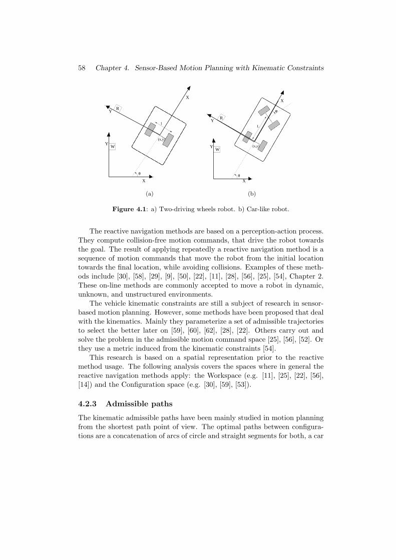
58 Chapter 4. Sensor-Based Motion Planning with Kinematic Constraints
Y
Y
(x,y)
l
W
θ
R
X
XX
Y
X
W
R
(x,y)
L
θ
φ
Y
(a) (b)
Figure 4.1: a) Two-driving wheels robot. b) Car-like robot.
The reactive navigation methods are based on a perception-action process.They compute collision-free motion commands, that drive the robot towardsthe goal. The result of applying repeatedly a reactive navigation method is asequence of motion commands that move the robot from the initial locationtowards the final location, while avoiding collisions. Examples of these meth-ods include [30], [58], [29], [9], [50], [22], [11], [28], [56], [25], [54], Chapter 2.These on-line methods are commonly accepted to move a robot in dynamic,unknown, and unstructured environments.
The vehicle kinematic constraints are still a subject of research in sensor-based motion planning. However, some methods have been proposed that dealwith the kinematics. Mainly they parameterize a set of admissible trajectoriesto select the better later on [59], [60], [62], [28], [22]. Others carry out andsolve the problem in the admissible motion command space [25], [56], [52]. Orthey use a metric induced from the kinematic constraints [54].
This research is based on a spatial representation prior to the reactivemethod usage. The following analysis covers the spaces where in general thereactive navigation methods apply: the Workspace (e.g. [11], [25], [22], [56],[14]) and the Configuration space (e.g. [30], [59], [53]).
4.2.3 Admissible paths
The kinematic admissible paths have been mainly studied in motion planningfrom the shortest path point of view. The optimal paths between configura-tions are a concatenation of arcs of circle and straight segments for both, a car
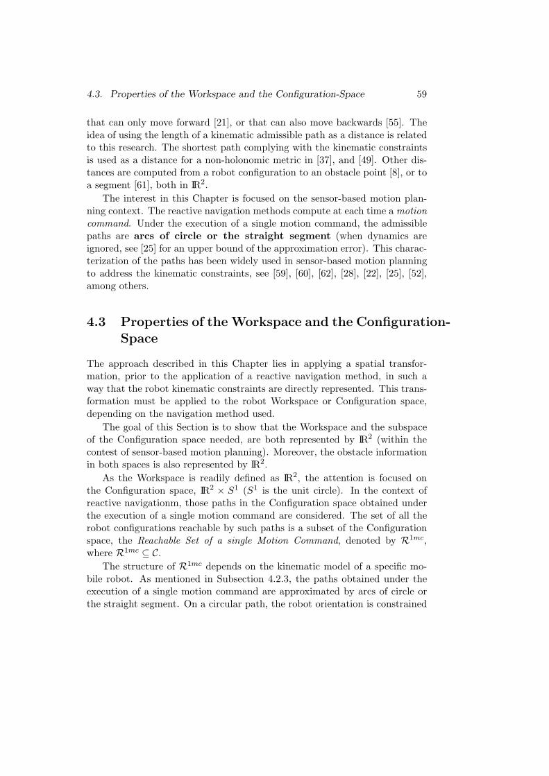
4.3. Properties of the Workspace and the Configuration-Space 59
that can only move forward [21], or that can also move backwards [55]. Theidea of using the length of a kinematic admissible path as a distance is relatedto this research. The shortest path complying with the kinematic constraintsis used as a distance for a non-holonomic metric in [37], and [49]. Other dis-tances are computed from a robot configuration to an obstacle point [8], or toa segment [61], both in IR2.
The interest in this Chapter is focused on the sensor-based motion plan-ning context. The reactive navigation methods compute at each time a motioncommand. Under the execution of a single motion command, the admissiblepaths are arcs of circle or the straight segment (when dynamics areignored, see [25] for an upper bound of the approximation error). This charac-terization of the paths has been widely used in sensor-based motion planningto address the kinematic constraints, see [59], [60], [62], [28], [22], [25], [52],among others.
4.3 Properties of the Workspace and the Configuration-Space
The approach described in this Chapter lies in applying a spatial transfor-mation, prior to the application of a reactive navigation method, in such away that the robot kinematic constraints are directly represented. This trans-formation must be applied to the robot Workspace or Configuration space,depending on the navigation method used.
The goal of this Section is to show that the Workspace and the subspaceof the Configuration space needed, are both represented by IR2 (within thecontest of sensor-based motion planning). Moreover, the obstacle informationin both spaces is also represented by IR2.
As the Workspace is readily defined as IR2, the attention is focused onthe Configuration space, IR2 × S1 (S1 is the unit circle). In the context ofreactive navigationm, those paths in the Configuration space obtained underthe execution of a single motion command are considered. The set of all therobot configurations reachable by such paths is a subset of the Configurationspace, the Reachable Set of a single Motion Command, denoted by R1mc,where R1mc ⊆ C.
The structure of R1mc depends on the kinematic model of a specific mo-bile robot. As mentioned in Subsection 4.2.3, the paths obtained under theexecution of a single motion command are approximated by arcs of circle orthe straight segment. On a circular path, the robot orientation is constrained
60 Chapter 4. Sensor-Based Motion Planning with Kinematic Constraints
by:
θ =
{atan( 2xy
x2+y2 ), |x| ≥ |y|π − atan( 2xy
x2+y2 ), |x| < |y| (4.3)
which is expressed in the robot frame of reference.Equation 4.3 is a holonomic equality constraint. The effect is to reduce
the dimension of the Configuration space by one [35]. Therefore, the ReachableSet of a single motion commandR1mc (i.e. the set of all the configurations thatcan be reached by the straight segment or one arc of a circle) is a function ofonly two parameters, and can be represented by IR2. A configuration in R1mc
is represented by q1mc = (x, y) (once (x, y) are selected, θ is given by Equation4.3.). Fig. 4.2 depicts how any point (x, y) of the space can be reached, butonly with one arc of a circle or the straight segment. The robot orientation ateach point (x, y) must be tangent to the arc of circle.
A point worth mentioning here is the fact that both, the robot Workspace,W, and the Reachable Set of a single Motion Command, R1mc, can be de-scribed by IR2.
For reactive navigation, the sensory information (obstacle information),that is usually given in the Workspace W, still needs to be mapped into theReachable Set of a single Motion Command R1mc.
The obstacles are represented in W by a set of points (x, y) ∈ IR2. This isa reasonable assumption since the sources of information are real sensors (e.g.the lasers measure points), and the environment is assumed to be unstructured(e.g. avoiding the use of polygons). Fig. 4.7d and Fig. 4.8d illustrate the typeof sensory information that is being dealt with. Then, each obstacle pointin W is mapped into a region in R1mc, called C-Obstacle [35]. The unionof the C-Obstacles is called the C-Obstacle region, R1mc
obs ⊂ R1mc. Fig. 4.8adepicts a differential-driven rectangular robot and the sensory information inW. The R1mc is illustrated in Fig. 4.8b. Notice that while C for this robot isthree-dimensional and so Cobs, the R1mc and R1mc
obs are two-dimensional.Appendix B presents an algorithm to compute a discretization of the R1mc
obs
boundary. To calculate the exact boundary remains an open problem. Theinterest is in a discretized version because: (1) in the following, a transfor-mation IR2 → IR2 is presented. Then other representations of the boundarymight be discretized to apply the transformation, or the transformation mightbe redesigned. And (2) the sensory information remains in the form of points,that is the input of most of the existing reactive navigation methods.
Summarizing, the robot Workspace, W, and the subset of the Configu-ration space needed, the Reachable Set of a single Motion Command, R1mc,
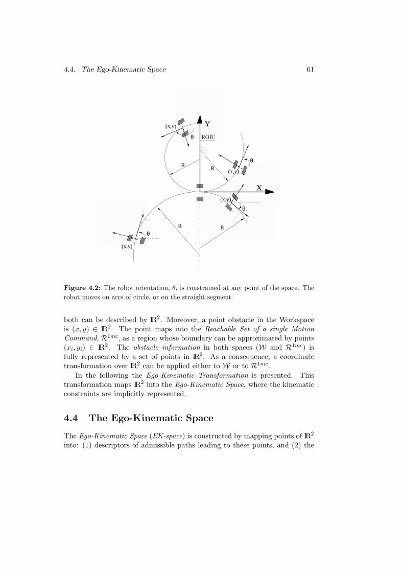
4.4. The Ego-Kinematic Space 61
θ
θ
θ
ROB
X
Y
θ
(x,y)
(x,y)
(x,y)
R R
RR
(x,y)
Figure 4.2: The robot orientation, θ, is constrained at any point of the space. Therobot moves on arcs of circle, or on the straight segment.
both can be described by IR2. Moreover, a point obstacle in the Workspaceis (x, y) ∈ IR2. The point maps into the Reachable Set of a single MotionCommand, R1mc, as a region whose boundary can be approximated by points(xi, yi) ∈ IR2. The obstacle information in both spaces (W and R1mc) isfully represented by a set of points in IR2. As a consequence, a coordinatetransformation over IR2 can be applied either to W or to R1mc.
In the following the Ego-Kinematic Transformation is presented. Thistransformation maps IR2 into the Ego-Kinematic Space, where the kinematicconstraints are implicitly represented.
4.4 The Ego-Kinematic Space
The Ego-Kinematic Space (EK-space) is constructed by mapping points of IR2
into: (1) descriptors of admissible paths leading to these points, and (2) the
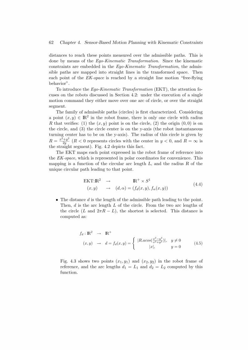
62 Chapter 4. Sensor-Based Motion Planning with Kinematic Constraints
distances to reach these points measured over the admissible paths. This isdone by means of the Ego-Kinematic Transformation. Since the kinematicconstraints are embedded in the Ego-Kinematic Transformation, the admis-sible paths are mapped into straight lines in the transformed space. Theneach point of the EK-space is reached by a straight line motion “free-flyingbehavior”.
To introduce the Ego-Kinematic Transformation (EKT), the attention fo-cuses on the robots discussed in Section 4.2: under the execution of a singlemotion command they either move over one arc of circle, or over the straightsegment.
The family of admissible paths (circles) is first characterized. Consideringa point (x, y) ∈ IR2 in the robot frame, there is only one circle with radiusR that verifies: (1) the (x, y) point is on the circle, (2) the origin (0, 0) is onthe circle, and (3) the circle center is on the y-axis (the robot instantaneousturning center has to be on the y-axis). The radius of this circle is given byR = x2+y2
2y (R < 0 represents circles with the center in y < 0, and R = ∞ isthe straight segment). Fig. 4.2 depicts this fact.
The EKT maps each point expressed in the robot frame of reference intothe EK-space, which is represented in polar coordinates for convenience. Thismapping is a function of the circular arc length L, and the radius R of theunique circular path leading to that point.
EKT:IR2 → IR+ × S1
(x, y) → (d, α) = (fd(x, y), fα(x, y))(4.4)
• The distance d is the length of the admissible path leading to the point.Then, d is the arc length L of the circle. From the two arc lengths ofthe circle (L and 2πR − L), the shortest is selected. This distance iscomputed as:
fd : IR2 → IR+
(x, y) → d = fd(x, y) =
{|R.acos(x2−y2
x2+y2 )|, y 6= 0
|x|, y = 0(4.5)
Fig. 4.3 shows two points (x1, y1) and (x2, y2) in the robot frame ofreference, and the arc lengths d1 = L1 and d2 = L2 computed by thisfunction.
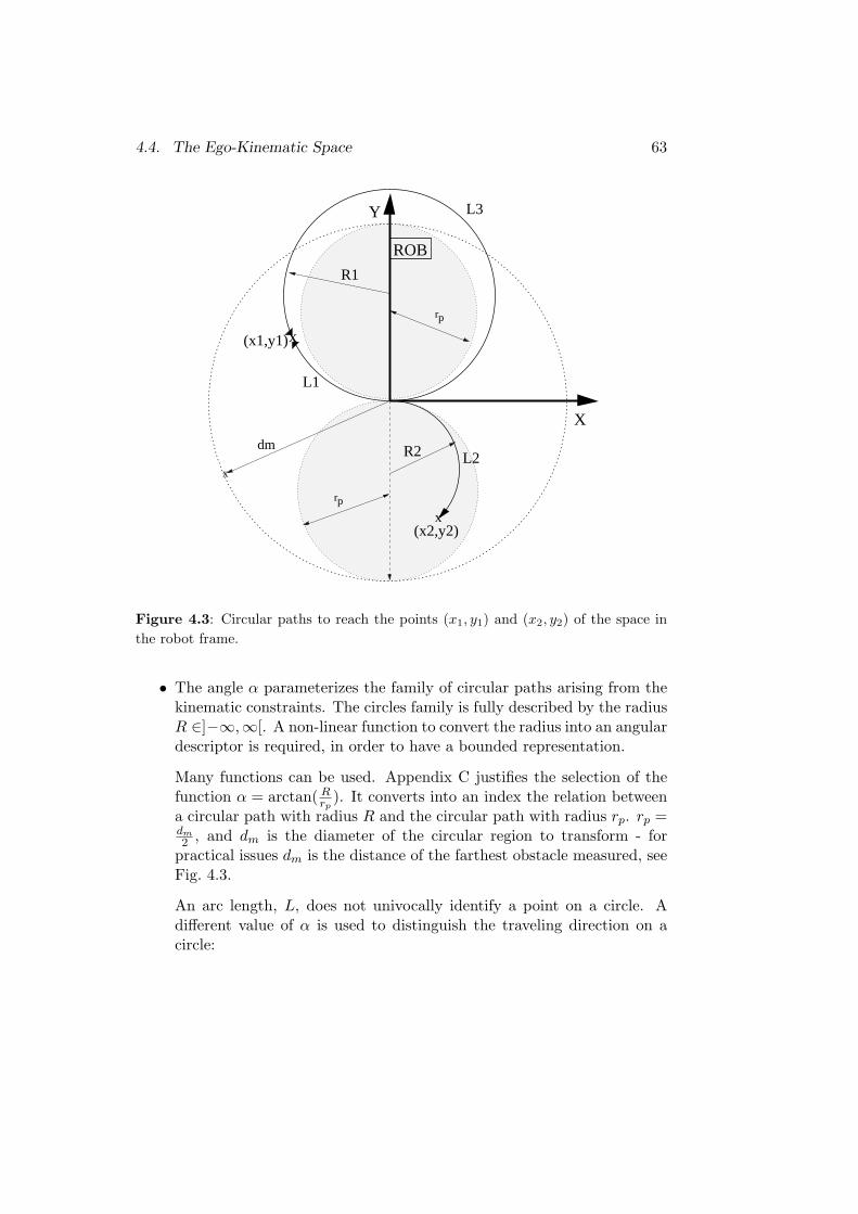
4.4. The Ego-Kinematic Space 63
pr
rp
x
Y
X
x
x
dm
(x2,y2)
L2R2
L1
R1
L3
(x1,y1)
ROB
Figure 4.3: Circular paths to reach the points (x1, y1) and (x2, y2) of the space inthe robot frame.
• The angle α parameterizes the family of circular paths arising from thekinematic constraints. The circles family is fully described by the radiusR ∈]−∞,∞[. A non-linear function to convert the radius into an angulardescriptor is required, in order to have a bounded representation.
Many functions can be used. Appendix C justifies the selection of thefunction α = arctan( R
rp). It converts into an index the relation between
a circular path with radius R and the circular path with radius rp. rp =dm2 , and dm is the diameter of the circular region to transform - for
practical issues dm is the distance of the farthest obstacle measured, seeFig. 4.3.
An arc length, L, does not univocally identify a point on a circle. Adifferent value of α is used to distinguish the traveling direction on acircle:
64 Chapter 4. Sensor-Based Motion Planning with Kinematic Constraints
fα : IR2 → [−π, π]
(x, y) → α = fα(x, y) = sign(x).π2 − arctan( R
rp) (4.6)
Fig. 4.4a shows an example of the EKT applied to a discrete set of pointsof a polygon. Each side of the polygon is numbered to notice how it trans-forms into the EK-space, illustrated in Fig. 4.4b. The angles α ∈]α1, π − α1[correspond to 0 < R < R1, whereas the angles α ∈]α2,−π − α2[ result from0 > R > R2. The values of α = 0 and α = π correspond to both, the straightforward and backward paths respectively along the x-axis.
Some points are worth mentioning here:
1. The EK-space can be computed in closed form.
2. The EKT is invertible. A pair (d, α) ∈ EK-space determines univocallya pair (x, y) ∈ IR2, and implicitly a θ ∈ S1.
3. The distance from the robot to any point in the EK-space is adequatelydescribed by the Euclidean distance. While this distance is the lengthof the admissible path that complies with the kinematic constraints.
4. The robot in the EK-space is a ”free flying object”, because it can movein any direction. Notice that a direction of motion α in the EK-spacesettles a unique turning radius for the robot, having R = f−1
α (α).
Next, the Ego-Kinematic Transformation is extended to consider the caseof robots that can only move forwards. Subsequently, the case of vehicles withcurvature constraints is analyzed.
4.4.1 Forward Motion Constraint
The EKT transforms each point into descriptors that univocally describe thepath leading to that point. So far circular paths have been considered, whereforward and backward motion were allowed. Here, the additional constraintto forbid backward motion is added. This is incorporated to the EKT byimposing a traveling direction over a circle. Fig. 4.3 depicts the idea: toreach (x1, y1), L3 is computed, instead of L1 that would be calculated by thestandard EKT.
The Ego-Kinematic Transformation then becomes:
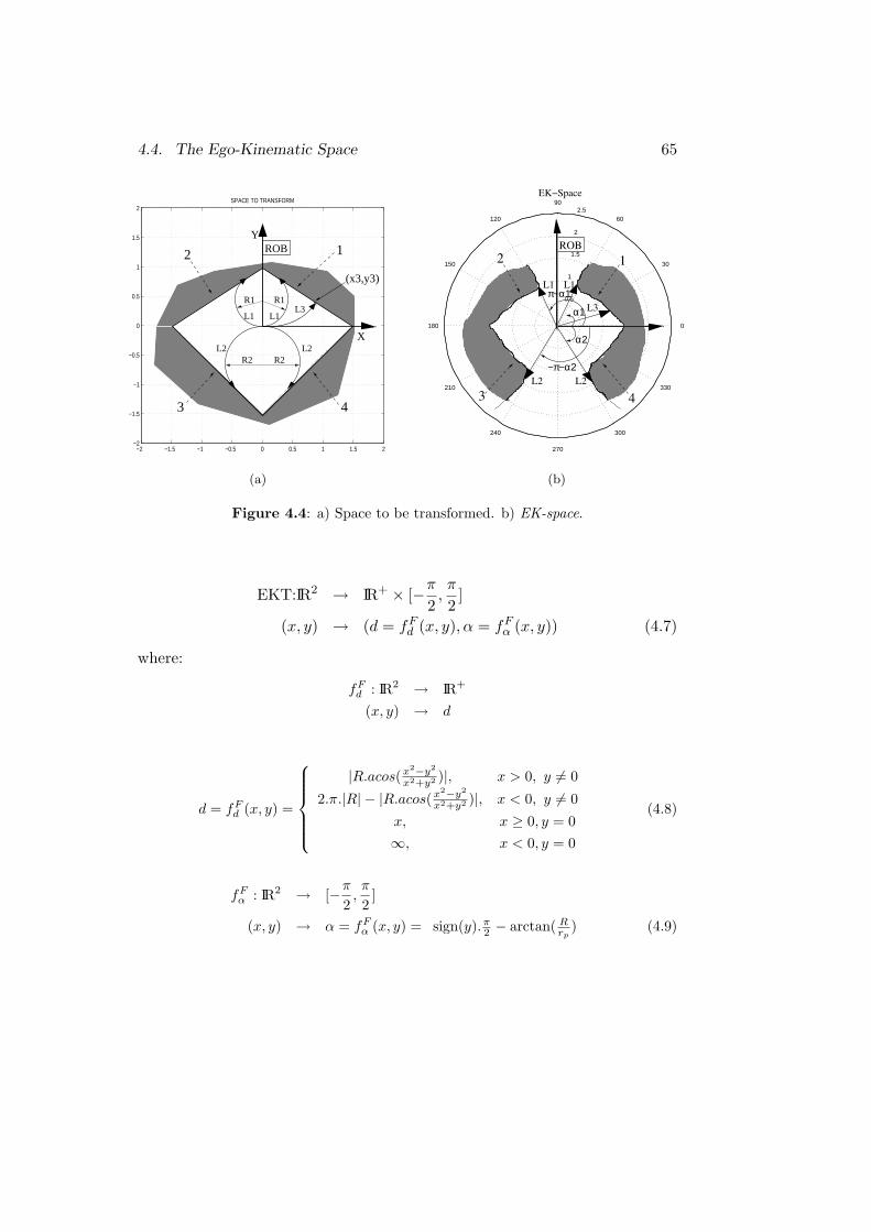
4.4. The Ego-Kinematic Space 65
−2 −1.5 −1 −0.5 0 0.5 1 1.5 2−2
−1.5
−1
−0.5
0
0.5
1
1.5
2SPACE TO TRANSFORM
R1 x
R2
Y
X
L3
R2
R1
L2 L2
L1L1
2
3
1
4
(x3,y3)
ROB
0.5
1
1.5
2
2.5
30
210
60
240
90
270
120
300
150
330
180 0
ROB
α1
L1
−π−α2
π−α1L3
L1
EK−Space
L2 L2
α2
2
3
1
4
(a) (b)
Figure 4.4: a) Space to be transformed. b) EK-space.
EKT:IR2 → IR+ × [−π
2,π
2]
(x, y) → (d = fFd (x, y), α = fF
α (x, y)) (4.7)
where:
fFd : IR2 → IR+
(x, y) → d
d = fFd (x, y) =
|R.acos(x2−y2
x2+y2 )|, x > 0, y 6= 0
2.π.|R| − |R.acos(x2−y2
x2+y2 )|, x < 0, y 6= 0
x, x ≥ 0, y = 0∞, x < 0, y = 0
(4.8)
fFα : IR2 → [−π
2,π
2]
(x, y) → α = fFα (x, y) = sign(y).π
2 − arctan( Rrp
) (4.9)
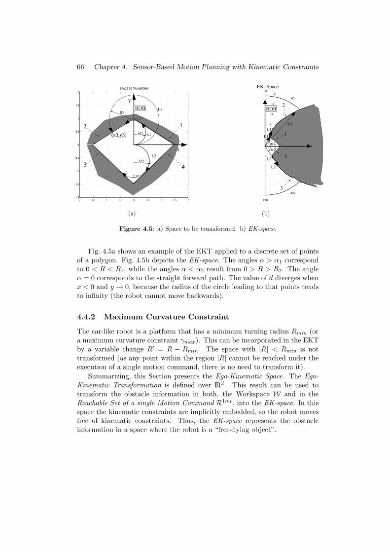
66 Chapter 4. Sensor-Based Motion Planning with Kinematic Constraints
−2 −1.5 −1 −0.5 0 0.5 1 1.5 2−2
−1.5
−1
−0.5
0
0.5
1
1.5
2SPACE TO TRANSFORM
ROB
1
43
2
Y
X
L1’
R3
R1
R2
L2’
L2
L3
L1(x3,y3) 1
2
3
4
5
30
210
60
240
90
270
120
300
150
330
180 0
L3
α1α2
L2
L2’
L1
L1’
3
4
1
2
EK−Space
ROB
(a) (b)
Figure 4.5: a) Space to be transformed. b) EK-space.
Fig. 4.5a shows an example of the EKT applied to a discrete set of pointsof a polygon. Fig. 4.5b depicts the EK-space. The angles α > α1 correspondto 0 < R < R1, while the angles α < α2 result from 0 > R > R2. The angleα = 0 corresponds to the straight forward path. The value of d diverges whenx < 0 and y → 0, because the radius of the circle leading to that points tendsto infinity (the robot cannot move backwards).
4.4.2 Maximum Curvature Constraint
The car-like robot is a platform that has a minimum turning radius Rmin (ora maximum curvature constraint γmax). This can be incorporated in the EKTby a variable change R′ = R − Rmin. The space with |R| < Rmin is nottransformed (as any point within the region |R| cannot be reached under theexecution of a single motion command, there is no need to transform it).
Summarizing, this Section presents the Ego-Kinematic Space. The Ego-Kinematic Transformation is defined over IR2. This result can be used totransform the obstacle information in both, the Workspace W and in theReachable Set of a single Motion Command R1mc, into the EK-space. In thisspace the kinematic constraints are implicitly embedded, so the robot movesfree of kinematic constraints. Thus, the EK-space represents the obstacleinformation in a space where the robot is a “free-flying object”.
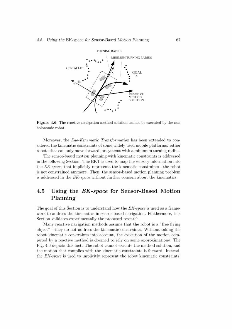
4.5. Using the EK-space for Sensor-Based Motion Planning 67
X
RY
REACTIVE METHODSOLUTION
OBSTACLES
MINIMUM TURNING RADIUS
XGOAL
TURNING RADIUS
Figure 4.6: The reactive navigation method solution cannot be executed by the nonholonomic robot.
Moreover, the Ego-Kinematic Transformation has been extended to con-sidered the kinematic constraints of some widely used mobile platforms: eitherrobots that can only move forward, or systems with a minimum turning radius.
The sensor-based motion planning with kinematic constraints is addressedin the following Section. The EKT is used to map the sensory information intothe EK-space, that implicitly represents the kinematic constraints - the robotis not constrained anymore. Then, the sensor-based motion planning problemis addressed in the EK-space without further concern about the kinematics.
4.5 Using the EK-space for Sensor-Based MotionPlanning
The goal of this Section is to understand how the EK-space is used as a frame-work to address the kinematics in sensor-based navigation. Furthermore, thisSection validates experimentally the proposed research.
Many reactive navigation methods assume that the robot is a ”free flyingobject” - they do not address the kinematic constraints. Without taking therobot kinematic constraints into account, the execution of the motion com-puted by a reactive method is doomed to rely on some approximations. TheFig. 4.6 depicts this fact. The robot cannot execute the method solution, andthe motion that complies with the kinematic constraints is forward. Instead,the EK-space is used to implicitly represent the robot kinematic constraints.
68 Chapter 4. Sensor-Based Motion Planning with Kinematic Constraints
Reactive navigation methods not designed for non-holonomic robots can beapplied to the EK-space. (Irrespective whether the method applies to theWorkspace or to the Configuration space.) Finally, the reactive navigationmethod solution in the EK-space is transformed back to the Workspace, tocompute an admissible motion command.
At each sample period T , the procedure to use the EK-space is the follow-ing:
1. The sensory information is reduced to points expressed in the robotframe of reference.
(a) If the reactive method applies to the Workspace W, the EKT isdirectly applied to the obstacle points.
(b) Or, if the reactive method applies to the Configuration space, theC-obstacle region R1mc
obs is first built (as described in Section 4.2),to apply the EKT.
In both cases the result is the obstacle information expressed in theEK-space.
2. The reactive navigation method is then applied to the EK-space to com-pute the most promising motion direction, α.
3. A turning radius is calculated by R = EKT−1(α). Finally, a motioncommand that preserves this turning radius is obtained by v = ω.R.
Any strategy to compute a pair (v, ω) that preserves R is valid. In thecurrent implementation v is calculated with the distance to the closest obstacle.Then, ω is computed. If ω > ωmax, then ω = ωmax and v is computedpreserving the turning radius R.
To validate this methodology experimentation with two different reactivenavigation methods has been conducted. Both methods do not take the kine-matic constraints into account. The reason to select the methods is to coveralmost all the results presented in the Chapter: firstly the Nearness DiagramNavigation, that applies to the Workspace and only allows forward motion.Secondly, the Potential Field Method, that applies to the Configuration spaceand allows both forward and backward motion.
Notice that the results obtained are not compared with other methods.The reason is that the scope of the Chapter is the spatial representation, notthe reactive method itself. The particular results are completely dependenton the reactive method used, and its specific implementation.
4.5. Using the EK-space for Sensor-Based Motion Planning 69
FREE WALKINGAREA
REGIONS
GAPS
GOALX
WORK SPACE
5 1
3
4
2OBSTACLE POINTS
TURNINGRADIUS
FREE WALKING
AREA
REGIONS
GAPS
1
2
5
4
3
XGOAL
EK−SPACE
ND SOLUTION
(a) (b)
x GOAL
0.8 meters
X GOAL
0.8 meters
(c) (d)
Figure 4.7: a)Workspace . b)EK-space. c) Experiment. d) Experiment.
4.5.1 Platform and Experimental Settings
The framework was tested in a Labmate robot at the University of Zaragoza,Spain. The main sensor is a 3D TRC laser rangefinder. For further detailsabout the robot and sensor, see Appendix E.0.5.
In all the experiments the environment was completely unknown, and onlythe goal location was given in advance to the robot. The environments wereunstructured (random shaped obstacles). Moreover, the environment couldbe dynamic and non-predictable. Under all these circumstances it is widelyjustified the use of sensor-based motion planning algorithms to move the robot.
70 Chapter 4. Sensor-Based Motion Planning with Kinematic Constraints
4.5.2 Nearness Diagram Navigation
The Nearness Diagram Navigation (ND), Chapter 2, is a reactive navigationmethod that does not take into account the kinematic constraints.
The ND method is described in detail in Chapter 2. However, a briefdescription of the method is next presented. The ND method is based on thesituated-activity methodology of design [3]. First, a set of five situations thatfully describe the relative state of the robot, obstacle distribution, and goallocation are defined. Subsequently, one action is designed for each situation.In real-time, the sensory information is used to identify the current situation,and the associated action is executed computing the motion commands.
To identify the current situation, in the sensory information some high levelinformation is searched for: gaps, regions, free walking areas. Some criteriaare also applied: a security criterion, a free walking area criterion, etc. Theindividual action designs are based on a geometrical implementation.
To apply the ND method to robots with kinematic constraints the EK-space is used.
At each sample period T the following procedure is repeated:
1. The EKT is applied to the sensory information in the Workspace (Fig.4.7a). The result is the obstacle information in the EK-space (Fig. 4.7b).
2. The ND method is applied to the EK-space to compute the most suitablemotion direction α∗ (represented in Fig. 4.7b as the ND solution). Someinformation used by the ND to compute the solution (the gaps, regions,and the free walking area, see Fig. 4.7a) is shown in Fig. 4.7b.
3. The direction α∗ is transformed back to the Workspace as a turningradius R∗ = EKT−1(α∗), see Fig. 4.7a. Finally, a motion command(v,w) that preserves this turning radius is computed.
This procedure was tested on the real robot. The cycle time of the al-gorithm (construction of the EK-space and reactive method usage) is around150msec on a 100MHz microSun SparcII. This execution time is enough forreal-time. Fig 4.7d shows a real experiment. The robot was safely driven tothe goal location - the only information given a priori to the robot. A circularrobot is drawn since a circle approximates the robot shape (due to ND imple-mentation requirements). Notice that the robot is safely driven among closedobstacles. The reason is that the ND method alone has been demonstratedto successfully drive platforms in dense, cluttered, and complex scenarios, seeChapters 2. The usage of the EK-space to address the kinematic constraints
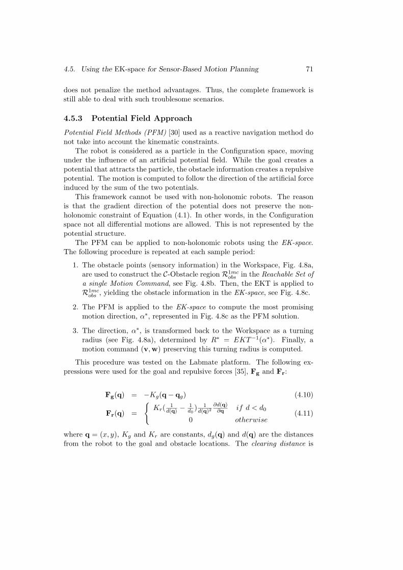
4.5. Using the EK-space for Sensor-Based Motion Planning 71
does not penalize the method advantages. Thus, the complete framework isstill able to deal with such troublesome scenarios.
4.5.3 Potential Field Approach
Potential Field Methods (PFM) [30] used as a reactive navigation method donot take into account the kinematic constraints.
The robot is considered as a particle in the Configuration space, movingunder the influence of an artificial potential field. While the goal creates apotential that attracts the particle, the obstacle information creates a repulsivepotential. The motion is computed to follow the direction of the artificial forceinduced by the sum of the two potentials.
This framework cannot be used with non-holonomic robots. The reasonis that the gradient direction of the potential does not preserve the non-holonomic constraint of Equation (4.1). In other words, in the Configurationspace not all differential motions are allowed. This is not represented by thepotential structure.
The PFM can be applied to non-holonomic robots using the EK-space.The following procedure is repeated at each sample period:
1. The obstacle points (sensory information) in the Workspace, Fig. 4.8a,are used to construct the C-Obstacle region R1mc
obs in the Reachable Set ofa single Motion Command, see Fig. 4.8b. Then, the EKT is applied toR1mc
obs , yielding the obstacle information in the EK-space, see Fig. 4.8c.
2. The PFM is applied to the EK-space to compute the most promisingmotion direction, α∗, represented in Fig. 4.8c as the PFM solution.
3. The direction, α∗, is transformed back to the Workspace as a turningradius (see Fig. 4.8a), determined by R∗ = EKT−1(α∗). Finally, amotion command (v,w) preserving this turning radius is computed.
This procedure was tested on the Labmate platform. The following ex-pressions were used for the goal and repulsive forces [35], Fg and Fr:
Fg(q) = −Kg(q− qg) (4.10)
Fr(q) =
{Kr( 1
d(q) − 1d0
) 1d(q)2
∂d(q)∂q if d < d0
0 otherwise(4.11)
where q = (x, y), Kg and Kr are constants, dg(q) and d(q) are the distancesfrom the robot to the goal and obstacle locations. The clearing distance is
72 Chapter 4. Sensor-Based Motion Planning with Kinematic Constraints
−2 −1.5 −1 −0.5 0 0.5 1 1.5 2 2.5 3−2
−1.5
−1
−0.5
0
0.5
1
1.5
2
2.5
3WORKING SPACE
TURNINGRADIUS
OBSTACLE POINTSROBOT
X
Y
GOAL
−2 −1.5 −1 −0.5 0 0.5 1 1.5 2 2.5 3−2
−1.5
−1
−0.5
0
0.5
1
1.5
2
2.5
3CONFIGURATION SPACE OF ONE MOTION COMMAND
X
Y
C-OBSTACLE
(a) (b)
1
2
3
30
210
60
240
90
270
120
300
150
330
180 0
EGO-KINEMATIC SPACE
PFM SOLUTION
GOAL
0.8 metersxGOAL
(c) (d)
Figure 4.8: (a) Workspace. (b) Reachable Set of a single motion command R1mcobs .
(c) EK-space. (d) Experimental result.
denoted by d0.∂d(q)
∂q represents the unit vector pointing away from the C-Obstacle region, and that is supported by the line passing through q and theobstacle point of the region.
Notice that the original potential formulation deals with the Configurationspace, that is IR2 × S1. Here, the potential is defined in the Reachable Set ofa single Motion Command, that is IR2. The subspace of the configurationneeded has one dimension less (as detailed in Section 4.3).
The execution time of the algorithm (construction of the Reachable Set ofa single Motion Command, EK-space, and reactive method usage) is around250msec. Hence this cycle-time was enough for real-time. Fig. 4.8d shows anexperiment performed with the real platform. The complete framework wasable to drive the constrained platform free of collisions to the goal location -
4.6. Conclusions 73
the only information given a priori to the robot. The experiment highlightsthe effect of the EK-space to address the kinematics: arcs of circle mainlycompose the motions computed and executed.
4.6 Conclusions
This Chapter addresses the sensor-based motion planning with kinematic con-straints. The novelty of the idea is to use the motion constraints to constructa spatial representation - Ego-Kinematic space. The kinematic constraintsare implicitly represented in this space, so the robot moves as a ”free-flyingobject”. Then, it is straightforward to use in this space existing reactivenavigation methods. Therefore, the method solutions comply with the kine-matic constraints. A wide solution to address the kinematic constraints in thesensor-based motion planning discipline has been presented.
The Configuration space for the robots covered in the analysis is IR2×S1.Another contribution is to show that only a subspace of the Configurationspace, IR2, is needed (in the context of sensor-based motion planning). Analgorithm to calculate the bounds of the C-Obstacle region in this subspaceis given. The author thinks that this result will alleviate the computationsrequired for reactive navigation methods in the future.
The proposed research has been validated experimentally with a real plat-form. By using the methodology, two reactive navigation methods were usedto successfully drive the constrained platform among locations. Both methodsare not originally formulated to work on non-holonomic robots.
Extensions to other non-holonomic robots are straightforward. The ad-missible paths that arise from their kinematic constraints would derive in newformulations of the Ego-Kinematic Transformation.
This research addresses the kinematic constraints, but ignores the effectof the dynamics. We have been working in a similar approach described indetail in Chapter 5: to introduce the dynamic constraints in the space. Ourobjective is to merge both works to address the sensor-based motion planningwith kinematic and dynamic constraints.

74 Chapter 4. Sensor-Based Motion Planning with Kinematic Constraints
Chapter 5
Sensor-Based MotionPlanning with DynamicConstraints
5.1 Introduction
The Robotic community is building robots for many fields and applications.Many of these applications require the safe motion generation: Service ro-bots, demining robots, healthcare robots, and supervision robots, among oth-ers. Some of these robots exhibit dynamic constraints due to the mechani-cal construction, or to the environment of application: robots with limitedtorques, robots working in non-gravity conditions, underwater robots, andblimps, among others. Moreover, some applications require moving the plat-forms at relatively high-speeds. In both cases the dynamic capabilities of therobot take an important place, constraining the feasible system motions.
This Chapter presents a framework to take into account the robot dynamicconstraints in the reactive collision avoidance layer. The proposal is to use thedynamic constraints to build a spatial representation, where the dynamic con-straints are implicitly represented. With minor modifications, many existingreactive navigation methods, that do not take the dynamic constraints into ac-count, can be applied to this space. As a consequence, the motion commandscomputed comply with the robot dynamics. This is an ample solution to incor-porate the dynamics into much of the current work developed in sensor-basedmotion planning.
The novelty is that the dynamic constraints are implicitly embedded in the
75
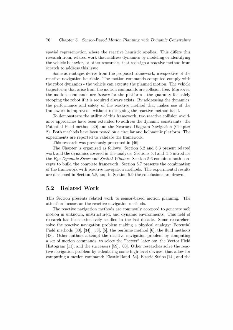
76 Chapter 5. Sensor-Based Motion Planning with Dynamic Constraints
spatial representation where the reactive heuristic applies. This differs thisresearch from, related work that address dynamics by modeling or identifyingthe vehicle behavior, or other researches that redesign a reactive method fromscratch to address this issue.
Some advantages derive from the proposed framework, irrespective of thereactive navigation heuristic. The motion commands computed comply withthe robot dynamics - the vehicle can execute the planned motion. The vehicletrajectories that arise from the motion commands are collision-free. Moreover,the motion commands are Secure for the platform - the guaranty for safelystopping the robot if it is required always exists. By addressing the dynamics,the performance and safety of the reactive method that makes use of theframework is improved - without redesigning the reactive method itself.
To demonstrate the utility of this framework, two reactive collision avoid-ance approaches have been extended to address the dynamic constraints: thePotential Field method [30] and the Nearness Diagram Navigation (Chapter2). Both methods have been tested on a circular and holonomic platform. Theexperiments are reported to validate the framework.
This research was previously presented in [46].The Chapter is organized as follows. Section 5.2 and 5.3 present related
work and the dynamics covered in the analysis. Sections 5.4 and 5.5 introducethe Ego-Dynamic Space and Spatial Window. Section 5.6 combines both con-cepts to build the complete framework. Section 5.7 presents the combinationof the framework with reactive navigation methods. The experimental resultsare discussed in Section 5.8, and in Section 5.9 the conclusions are drawn.
5.2 Related Work
This Section presents related work to sensor-based motion planning. Theattention focuses on the reactive navigation methods.
The reactive navigation methods are commonly accepted to generate safemotion in unknown, unstructured, and dynamic environments. This field ofresearch has been extensively studied in the last decade. Some researcherssolve the reactive navigation problem making a physical analogy: PotentialField methods [30], [34], [58], [5]; the perfume method [6], the fluid methods[43]. Other authors attempt the reactive navigation problem by computinga set of motion commands, to select the ”better” later on: the Vector FieldHistogram [11], and the successors [59], [60]. Other researches solve the reac-tive navigation problem by calculating some high-level devices, that allow forcomputing a motion command: Elastic Band [54], Elastic Strips [14], and the
5.3. Dynamics in Motion Commands 77
Nearness Diagram Navigation (Chapter 2).Most of the reactive navigation methods do not address dynamics. Thus,
these methods are susceptible to failure in the case analyzed in this Chapter.The dynamic constraints have been mainly addressed in sensor-based motionplanning from two different points of view: (1) some researches deal withdynamics by modeling the system behavior. Some of them model the system[31], [5], [16]. Others identify the system model by the responses to motioncommands (inputs) [2], [40]. Once the model is available, the system responsesare also known, and used to apply reactive navigation strategies. (2) Someauthors explain the system response with a model of constrained inputs. Someof them solve the reactive navigation problem in the motion command space asa constrained optimization [56], [25], [13]. Others compute dynamic admissibletrajectories, to obtain the motion commands later on [22], [62].
The spaces where the reactive navigation methods usually apply are theWorkspace W, [44], [14], [50], [6], [43], [11]; or the Configuration space C[35], [30], [34], [58], [59], [60], [54]. The research presented here is basedon a spatial representation - prior to the reactive method usage - where thesystem dynamics are implicitly represented. Then, both spaces, W and C, areanalyzed to achieve the maximum generality.
5.3 Dynamics in Motion Commands
This Section first analyses the vehicle case of study. Subsection 5.3.2 presentsthe motion commands considered, and in Subsection 5.3.3 the dynamics in-volved in the motion command execution are discussed.
5.3.1 Vehicle
The vehicle considered is a circular and holonomic robot moving on a flat sur-face with the classical hypothesis “rolling without slipping”. The WorkspaceW is IR2. The Configuration space C is IR2 × S1. Since the robot is circular,the Configuration space can projected in IR2. Then both, the Workspace andthe Configuration space are represented by IR2. The space of motion com-mands is three-dimensional, where (v,w) is a motion command. v = (vx, vy)is the translational velocity, and w is the rotational velocity. Both velocitiesexpressed in the robot reference system. The attention focuses on v = (vx, vy)because it modifies the robot location (the robot rotational velocity, w, is notdependent on the translational velocity).
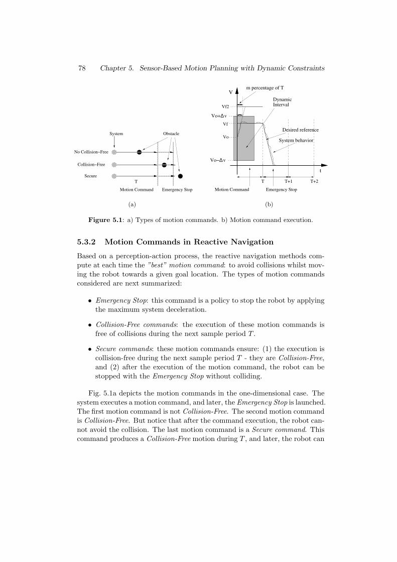
78 Chapter 5. Sensor-Based Motion Planning with Dynamic Constraints
T
Motion Command Emergency Stop
ObstacleSystem
No Collision−Free
Collision−Free
Secure
DynamicInterval
T T+1 T+2
V
Vf
Vo
Vf2
Vo+ v∆
Vo− v∆
t
System behavior
Desired reference
m percentage of T
Motion Command Emergency Stop
(a) (b)
Figure 5.1: a) Types of motion commands. b) Motion command execution.
5.3.2 Motion Commands in Reactive Navigation
Based on a perception-action process, the reactive navigation methods com-pute at each time the ”best” motion command: to avoid collisions whilst mov-ing the robot towards a given goal location. The types of motion commandsconsidered are next summarized:
• Emergency Stop: this command is a policy to stop the robot by applyingthe maximum system deceleration.
• Collision-Free commands: the execution of these motion commands isfree of collisions during the next sample period T .
• Secure commands: these motion commands ensure: (1) the execution iscollision-free during the next sample period T - they are Collision-Free,and (2) after the execution of the motion command, the robot can bestopped with the Emergency Stop without colliding.
Fig. 5.1a depicts the motion commands in the one-dimensional case. Thesystem executes a motion command, and later, the Emergency Stop is launched.The first motion command is not Collision-Free. The second motion commandis Collision-Free. But notice that after the command execution, the robot can-not avoid the collision. The last motion command is a Secure command. Thiscommand produces a Collision-Free motion during T , and later, the robot can
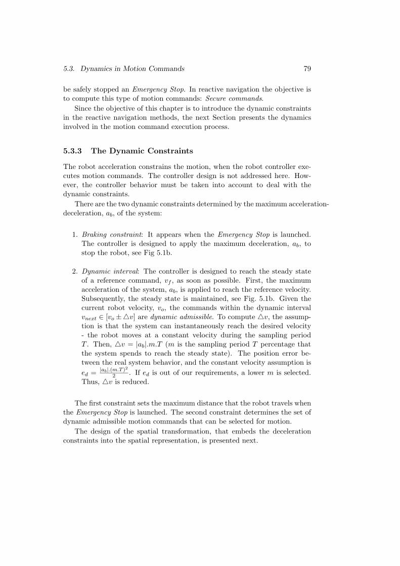
5.3. Dynamics in Motion Commands 79
be safely stopped an Emergency Stop. In reactive navigation the objective isto compute this type of motion commands: Secure commands.
Since the objective of this chapter is to introduce the dynamic constraintsin the reactive navigation methods, the next Section presents the dynamicsinvolved in the motion command execution process.
5.3.3 The Dynamic Constraints
The robot acceleration constrains the motion, when the robot controller exe-cutes motion commands. The controller design is not addressed here. How-ever, the controller behavior must be taken into account to deal with thedynamic constraints.
There are the two dynamic constraints determined by the maximum acceleration-deceleration, ab, of the system:
1. Braking constraint: It appears when the Emergency Stop is launched.The controller is designed to apply the maximum deceleration, ab, tostop the robot, see Fig 5.1b.
2. Dynamic interval: The controller is designed to reach the steady stateof a reference command, vf , as soon as possible. First, the maximumacceleration of the system, ab, is applied to reach the reference velocity.Subsequently, the steady state is maintained, see Fig. 5.1b. Given thecurrent robot velocity, vo, the commands within the dynamic intervalvnext ∈ [vo ±4v] are dynamic admissible. To compute 4v, the assump-tion is that the system can instantaneously reach the desired velocity- the robot moves at a constant velocity during the sampling periodT . Then, 4v = |ab|.m.T (m is the sampling period T percentage thatthe system spends to reach the steady state). The position error be-tween the real system behavior, and the constant velocity assumption ised = |ab|.(m.T )2
2 . If ed is out of our requirements, a lower m is selected.Thus, 4v is reduced.
The first constraint sets the maximum distance that the robot travels whenthe Emergency Stop is launched. The second constraint determines the set ofdynamic admissible motion commands that can be selected for motion.
The design of the spatial transformation, that embeds the decelerationconstraints into the spatial representation, is presented next.
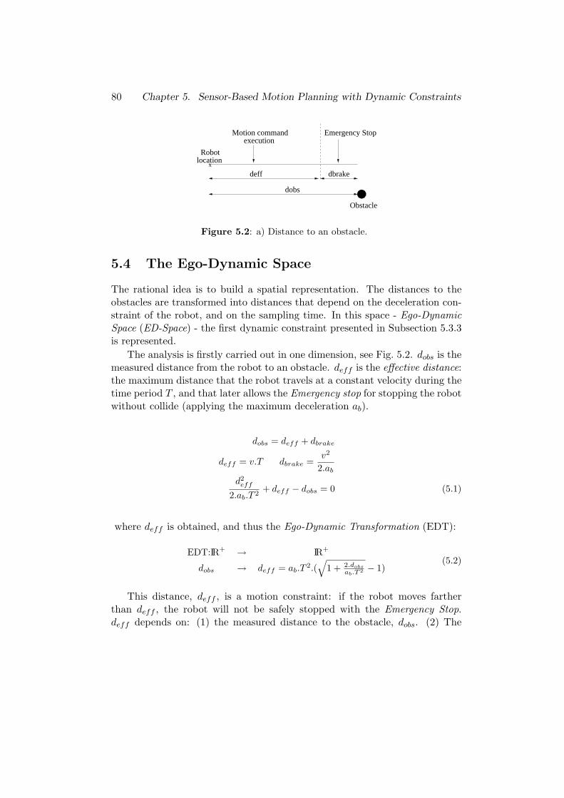
80 Chapter 5. Sensor-Based Motion Planning with Dynamic Constraints
location
deff
dobs
executionEmergency Stop
x
dbrake
Obstacle
Robot
Motion command
Figure 5.2: a) Distance to an obstacle.
5.4 The Ego-Dynamic Space
The rational idea is to build a spatial representation. The distances to theobstacles are transformed into distances that depend on the deceleration con-straint of the robot, and on the sampling time. In this space - Ego-DynamicSpace (ED-Space) - the first dynamic constraint presented in Subsection 5.3.3is represented.
The analysis is firstly carried out in one dimension, see Fig. 5.2. dobs is themeasured distance from the robot to an obstacle. deff is the effective distance:the maximum distance that the robot travels at a constant velocity during thetime period T , and that later allows the Emergency stop for stopping the robotwithout collide (applying the maximum deceleration ab).
dobs = deff + dbrake
deff = v.T dbrake =v2
2.ab
d2eff
2.ab.T 2+ deff − dobs = 0 (5.1)
where deff is obtained, and thus the Ego-Dynamic Transformation (EDT):
EDT:IR+ → IR+
dobs → deff = ab.T2.(
√1 + 2.dobs
ab.T 2 − 1)(5.2)
This distance, deff , is a motion constraint: if the robot moves fartherthan deff , the robot will not be safely stopped with the Emergency Stop.deff depends on: (1) the measured distance to the obstacle, dobs. (2) The
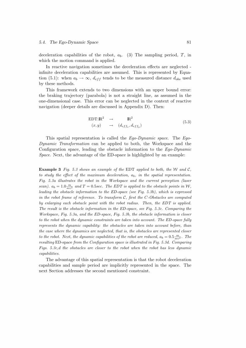
5.4. The Ego-Dynamic Space 81
deceleration capabilities of the robot, ab. (3) The sampling period, T , inwhich the motion command is applied.
In reactive navigation sometimes the deceleration effects are neglected -infinite deceleration capabilities are assumed. This is represented by Equa-tion (5.1): when ab → ∞, deff tends to be the measured distance dobs usedby these methods.
This framework extends to two dimensions with an upper bound error:the braking trajectory (parabola) is not a straight line, as assumed in theone-dimensional case. This error can be neglected in the context of reactivenavigation (deeper details are discussed in Appendix D). Then:
EDT:IR2 → IR2
(x, y) → (deffx, deffy
)(5.3)
This spatial representation is called the Ego-Dynamic space. The Ego-Dynamic Transformation can be applied to both, the Workspace and theConfiguration space, leading the obstacle information to the Ego-DynamicSpace. Next, the advantage of the ED-space is highlighted by an example:
Example 3 Fig. 5.3 shows an example of the EDT applied to both, the W and C,to study the effect of the maximum deceleration, ab, in the spatial representation.Fig. 5.3a illustrates the robot in the Workspace and the current perception (laserscan). ab = 1.0 m
sec2 and T = 0.5sec. The EDT is applied to the obstacle points in W,leading the obstacle information to the ED-space (see Fig. 5.3b), which is expressedin the robot frame of reference. To transform C, first the C-Obstacles are computedby enlarging each obstacle point with the robot radius. Then, the EDT is applied.The result is the obstacle information in the ED-space, see Fig. 5.3c. Comparing theWorkspace, Fig. 5.3a, and the ED-space, Fig. 5.3b, the obstacle information is closerto the robot when the dynamic constraints are taken into account. The ED-space fullyrepresents the dynamic capability: the obstacles are taken into account before, thanthe case where the dynamics are neglected, that is, the obstacles are represented closerto the robot. Next, the dynamic capabilities of the robot are reduced, ab = 0.5 m
sec2 . Theresulting ED-space from the Configuration space is illustrated in Fig. 5.3d. ComparingFigs. 5.3c,d the obstacles are closer to the robot when the robot has less dynamiccapabilities.
The advantage of this spatial representation is that the robot decelerationcapabilities and sample period are implicitly represented in the space. Thenext Section addresses the second mentioned constraint.
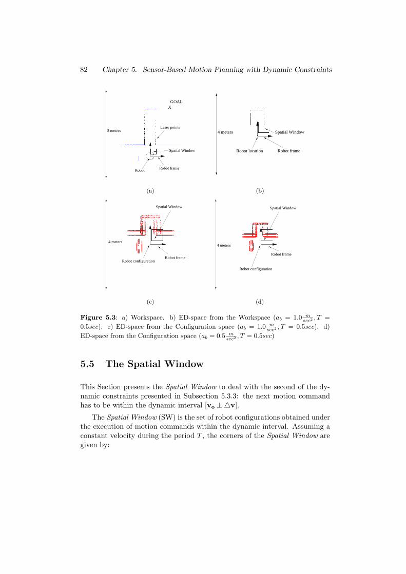
82 Chapter 5. Sensor-Based Motion Planning with Dynamic Constraints
Laser points
Robot Robot frame
8 meters
Spatial Window
XGOAL
Robot location Robot frame
4 meters Spatial Window
(a) (b)
Robot configurationRobot frame
4 meters
Spatial Window
4 meters
Robot configuration
Robot frame
Spatial Window
(c) (d)
Figure 5.3: a) Workspace. b) ED-space from the Workspace (ab = 1.0 msec2 , T =
0.5sec). c) ED-space from the Configuration space (ab = 1.0 msec2 , T = 0.5sec). d)
ED-space from the Configuration space (ab = 0.5 msec2 , T = 0.5sec)
5.5 The Spatial Window
This Section presents the Spatial Window to deal with the second of the dy-namic constraints presented in Subsection 5.3.3: the next motion commandhas to be within the dynamic interval [vo ±4v].
The Spatial Window (SW) is the set of robot configurations obtained underthe execution of motion commands within the dynamic interval. Assuming aconstant velocity during the period T , the corners of the Spatial Window aregiven by:
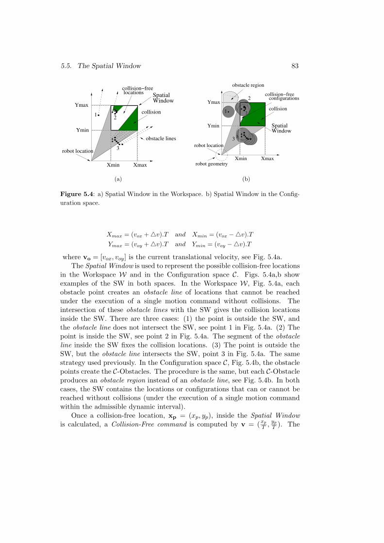
5.5. The Spatial Window 83
1collision
locations
XmaxXmin
obstacle lines
2
3robot location
collision−free
SpatialWindow
Ymax
Ymin
robot location
1 2
3
collision
2
3
robot geometryXmaxXmin
collision−free
obstacle region
WindowSpatialYmin
Ymaxconfigurations
(a) (b)
Figure 5.4: a) Spatial Window in the Workspace. b) Spatial Window in the Config-uration space.
Xmax = (vox +4v).T and Xmin = (vox −4v).TYmax = (voy +4v).T and Ymin = (voy −4v).T
where vo = [vox, voy] is the current translational velocity, see Fig. 5.4a.The Spatial Window is used to represent the possible collision-free locations
in the Workspace W and in the Configuration space C. Figs. 5.4a,b showexamples of the SW in both spaces. In the Workspace W, Fig. 5.4a, eachobstacle point creates an obstacle line of locations that cannot be reachedunder the execution of a single motion command without collisions. Theintersection of these obstacle lines with the SW gives the collision locationsinside the SW. There are three cases: (1) the point is outside the SW, andthe obstacle line does not intersect the SW, see point 1 in Fig. 5.4a. (2) Thepoint is inside the SW, see point 2 in Fig. 5.4a. The segment of the obstacleline inside the SW fixes the collision locations. (3) The point is outside theSW, but the obstacle line intersects the SW, point 3 in Fig. 5.4a. The samestrategy used previously. In the Configuration space C, Fig. 5.4b, the obstaclepoints create the C-Obstacles. The procedure is the same, but each C-Obstacleproduces an obstacle region instead of an obstacle line, see Fig. 5.4b. In bothcases, the SW contains the locations or configurations that can or cannot bereached without collisions (under the execution of a single motion commandwithin the admissible dynamic interval).
Once a collision-free location, xp = (xp, yp), inside the Spatial Windowis calculated, a Collision-Free command is computed by v = (xp
T ,yp
T ). The
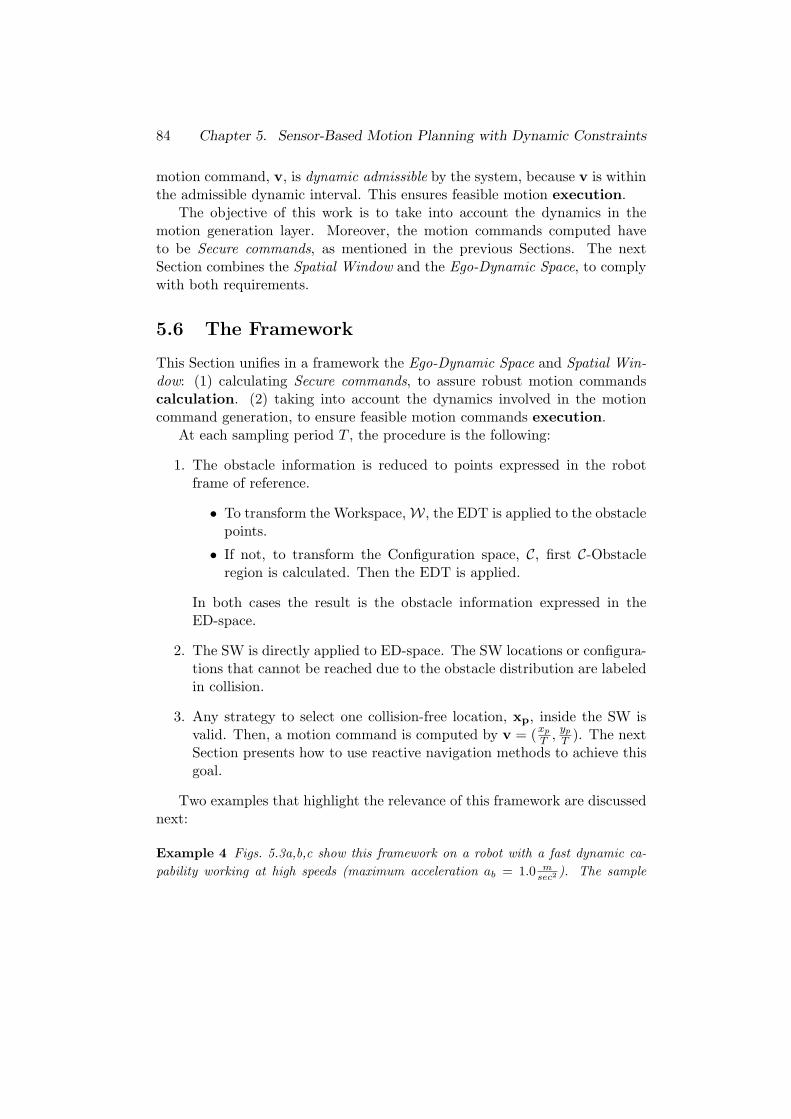
84 Chapter 5. Sensor-Based Motion Planning with Dynamic Constraints
motion command, v, is dynamic admissible by the system, because v is withinthe admissible dynamic interval. This ensures feasible motion execution.
The objective of this work is to take into account the dynamics in themotion generation layer. Moreover, the motion commands computed haveto be Secure commands, as mentioned in the previous Sections. The nextSection combines the Spatial Window and the Ego-Dynamic Space, to complywith both requirements.
5.6 The Framework
This Section unifies in a framework the Ego-Dynamic Space and Spatial Win-dow: (1) calculating Secure commands, to assure robust motion commandscalculation. (2) taking into account the dynamics involved in the motioncommand generation, to ensure feasible motion commands execution.
At each sampling period T , the procedure is the following:
1. The obstacle information is reduced to points expressed in the robotframe of reference.
• To transform the Workspace, W, the EDT is applied to the obstaclepoints.
• If not, to transform the Configuration space, C, first C-Obstacleregion is calculated. Then the EDT is applied.
In both cases the result is the obstacle information expressed in theED-space.
2. The SW is directly applied to ED-space. The SW locations or configura-tions that cannot be reached due to the obstacle distribution are labeledin collision.
3. Any strategy to select one collision-free location, xp, inside the SW isvalid. Then, a motion command is computed by v = (xp
T ,yp
T ). The nextSection presents how to use reactive navigation methods to achieve thisgoal.
Two examples that highlight the relevance of this framework are discussednext:
Example 4 Figs. 5.3a,b,c show this framework on a robot with a fast dynamic ca-pability working at high speeds (maximum acceleration ab = 1.0 m
sec2 ). The sample
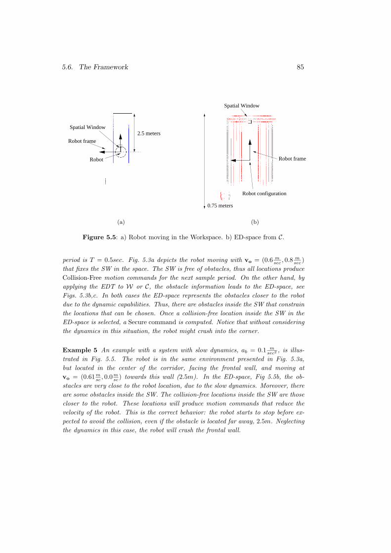
5.6. The Framework 85
Robot
Robot frame2.5 meters
Spatial Window
Robot configuration
Robot frame
0.75 meters
Spatial Window
(a) (b)
Figure 5.5: a) Robot moving in the Workspace. b) ED-space from C.
period is T = 0.5sec. Fig. 5.3a depicts the robot moving with vo = (0.6 msec , 0.8 m
sec )that fixes the SW in the space. The SW is free of obstacles, thus all locations produceCollision-Free motion commands for the next sample period. On the other hand, byapplying the EDT to W or C, the obstacle information leads to the ED-space, seeFigs. 5.3b,c. In both cases the ED-space represents the obstacles closer to the robotdue to the dynamic capabilities. Thus, there are obstacles inside the SW that constrainthe locations that can be chosen. Once a collision-free location inside the SW in theED-space is selected, a Secure command is computed. Notice that without consideringthe dynamics in this situation, the robot might crash into the corner.
Example 5 An example with a system with slow dynamics, ab = 0.1 msec2 , is illus-
trated in Fig. 5.5. The robot is in the same environment presented in Fig. 5.3a,but located in the center of the corridor, facing the frontal wall, and moving atvo = (0.61m
sc , 0.0msc ) towards this wall (2.5m). In the ED-space, Fig 5.5b, the ob-
stacles are very close to the robot location, due to the slow dynamics. Moreover, thereare some obstacles inside the SW. The collision-free locations inside the SW are thosecloser to the robot. These locations will produce motion commands that reduce thevelocity of the robot. This is the correct behavior: the robot starts to stop before ex-pected to avoid the collision, even if the obstacle is located far away, 2.5m. Neglectingthe dynamics in this case, the robot will crash the frontal wall.
86 Chapter 5. Sensor-Based Motion Planning with Dynamic Constraints
In this framework all locations inside the SW can be in collision. Then,the Emergency Stop is launched to safely stop the robot. Subsequently, themotion is resumed.
The main interests of the - ED-space + SW - framework are:
1. The motion commands are Secure commands, because they are com-puted from locations in the ED-space.
2. The motion commands comply with the system dynamics. They arewithin the dynamic interval vnext = [vo±4v], because the SW is used.
The next Section presents one strategy to select a location inside the SW,implicitly fixing the motion command.
5.7 Combining the Framework and the Reactive Nav-igation Methods
The framework presented in the previous Section leaves open the problem ofselecting one location inside the SW. This Section presents a solution basedon reactive navigation methods.
Notice that any strategy to select one collision-free location inside the SWsolves the problem. [25], [13], and [56] solve a similar problem by a constrainedoptimization that balances the goal location, the forward progress, and theobstacle clearance. Similar strategies could be used.
The solution here is to use existing reactive navigation methods in theED-space, to select a collision-free location inside the SW. The reasons forchoosing these techniques are:
1. The presented framework has to work in real-time. The usage of areactive method does not impose a significant time penalty. Everything-ED-space + SW + Reactive method - can be run in real-time.
2. The reactive navigation methods take directly into account the goal lo-cation; and information about the obstacle spatial distribution - thisadvantage is lost when the problem is solved with other types of heuris-tics, e.g. with a constrained optimization as [25], [13], [56].
3. The reactive navigation method is a module not dependent on the restof the framework. Different reactive methods can be used and testedwithin the framework without significant changes.
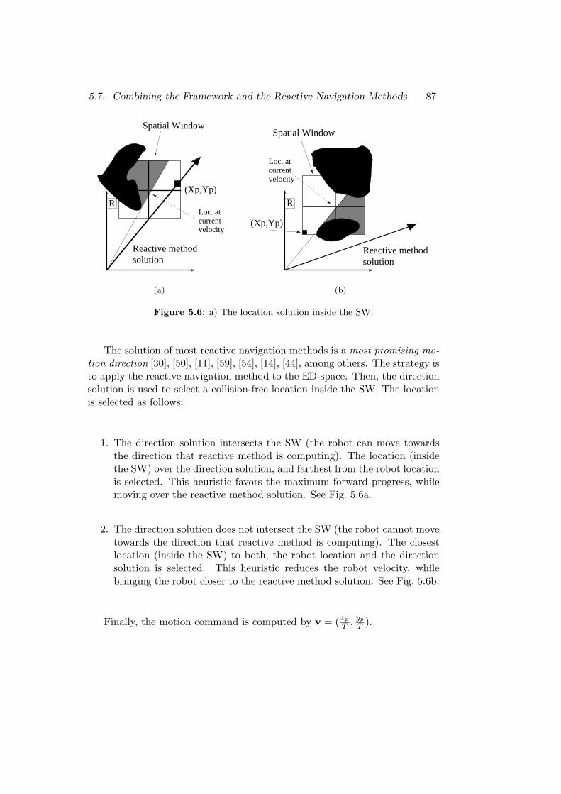
5.7. Combining the Framework and the Reactive Navigation Methods 87
Reactive methodsolution
R
(Xp,Yp)
Spatial Window
Loc. atcurrentvelocity
Reactive methodsolution
R
(Xp,Yp)
Spatial Window
Loc. atcurrent velocity
(a) (b)
Figure 5.6: a) The location solution inside the SW.
The solution of most reactive navigation methods is a most promising mo-tion direction [30], [50], [11], [59], [54], [14], [44], among others. The strategy isto apply the reactive navigation method to the ED-space. Then, the directionsolution is used to select a collision-free location inside the SW. The locationis selected as follows:
1. The direction solution intersects the SW (the robot can move towardsthe direction that reactive method is computing). The location (insidethe SW) over the direction solution, and farthest from the robot locationis selected. This heuristic favors the maximum forward progress, whilemoving over the reactive method solution. See Fig. 5.6a.
2. The direction solution does not intersect the SW (the robot cannot movetowards the direction that reactive method is computing). The closestlocation (inside the SW) to both, the robot location and the directionsolution is selected. This heuristic reduces the robot velocity, whilebringing the robot closer to the reactive method solution. See Fig. 5.6b.
Finally, the motion command is computed by v = (xp
T ,yp
T ).
88 Chapter 5. Sensor-Based Motion Planning with Dynamic Constraints
5.8 Experimental Results
This Section validates experimentally the proposed research. Experimentswere conducted with two reactive navigation methods: the Nearness DiagramNavigation [44], that applies to the Workspace W. Secondly, the PotentialField Method [30], that applies to the Configuration space C. Both methodsdo not take into account the dynamic constraints. By using the proposedframework, the vehicle dynamics are directly addressed.
Notice that the experimental results obtained are not compared to othermethods. The scope of the Chapter is the complete framework - ED-space +SW + Reactive method, and not the reactive method itself. The particularresults are completely dependent on the reactive method used and its specificimplementation.
However, the difference of the each reactive method behavior, when usingor not the proposed framework, is discussed. The benefits of using the reactivemethod with the framework are: (1) the motion commands computed are Se-cure motions: they are collision-free in execution, and they give the guarantyfor safely stopping the robot without collisions. (2) The motion command aredynamic feasible. Both benefits are not dependent on the navigation heuristicused. Then, the comparison is not directed in quantitative terms, since theusage of the framework improves the method behavior. The comparison is di-rected in qualitative terms: it was tested how far the fact of ignoring dynamics,produces motions that are not the planned ones - collision avoidance cannotbe guaranteed. This comparison demonstrates the robustness and quality ofthe approach. Moreover, other issues as global execution time are discussed.
The same environment, robot, and sensor were used for the method com-parison. However, it is very difficult to have the same navigation results intwo different trials, since real systems are used.
For experimentation was used a Nomadic XR4000 at LAAS-CNRS, France.The robot is equipped with a SICK 2-D laser rangefinder. See Appendix E.0.4for a deeper description of the robot and sensor.
5.8.1 Nearness Diagram Navigation
The Nearness Diagram Navigation (ND) [44] is a reactive navigation methodthat does not take into account the dynamic constraints.
The ND method is described in detail in Chapter 2. However, a briefintroduction to the method is next presented. The ND method is based on thesituated-activity methodology of design [3]. First, a set of five situations thatfully describe the relative state of the robot, obstacle distribution, and goal
5.8. Experimental Results 89
location are defined. Subsequently, one action is designed for each situation.In real-time, the sensory information is used to identify the current situation,and the associated action is executed computing the motion commands.
To identify the current situation, some high level information is searchedfor in the sensory information: gaps, regions, free walking areas. And somecriteria are also applied: a security criterion, a free walking area criterion, etc.The individual action designs are based on a geometrical implementation.
Using the proposed framework, the ND is used taking into account the dy-namic constraints. At each sample period the following procedure is repeated:
1. The EDT is applied to the sensory information in the Workspace (laserscan). The result is the obstacle information in the ED-space. (Proce-dure presented in Section 5.4)
2. The SW is filled using the obstacle information in the ED-space. (Pro-cedure presented in Section 5.5)
3. The ND method is applied to the ED-space to compute the most suitablemotion direction α∗. This direction α∗ is used to select a collision-free location, xp, inside the SW. (Procedure presented in Section 5.6).Finally, a motion command is computed by v = (xp
T ,yp
T ).
The procedure was tested on the real platform. Fig. 5.7a shows the resultof one of the runs. The robot successfully reached the goal location whileavoiding collisions with the environment. Figs. 5.7c,d depict the behavior ofthe system during the experiment: the motion commands reference computedby the framework (vx and vy), and the real ones executed by the robot (forbetter appreciation only a fraction of the experiment is shown). Notice that thesystem can execute the computed commands (the velocity error is illustratedin Fig. 5.7e). The consequence is that the trajectories carried out are nearto the planned ones: by addressing dynamics, robust collision avoidance isguarantied. On the other hand, the same experiment was carried out with thereactive method alone (ND). The velocity profile is illustrated in Fig. 5.7f,g.The system could not correctly execute the computed commands (the velocityerror is illustrated in Fig. 5.7h. The consequence is that the trajectories carriedout are distant from the planned ones: collision avoidance can be no longerguaranteed. More experiments were run to characterize the velocity errorprofile, see Fig. 5.7b. The error distribution gives the idea of the error in theexecuted trajectories.
Notice that the robot is safely driven among close obstacles, Fig. 5.7a.The reason is that the ND method alone has been demonstrated to successfully
90 Chapter 5. Sensor-Based Motion Planning with Dynamic Constraints
drive platforms in dense, cluttered, and complex scenarios, see Chapter 3. Theusage of the ED-space to address the dynamic constraints does not penalizethe method advantages. Thus, the complete framework is still able to dealwith troublesome scenarios.
From a global point of view, using the framework improves the safety ofthe method: the trajectories executed are near to the computed ones. Beyond,the framework gives the guaranty for safely stopping the robot if required. Thedrawback is the global execution time. The same experiments took about twoor three times longer that the ones without the dynamic considerations. Thereason is that the framework is very conservative. Only Secure velocities arecomputed. They usually penalize the acceleration because safety is prioritized.
5.8.2 Potential Field Method
Potential Field Methods (PFM) [30] can be used as reactive navigation meth-ods, but they do not take the dynamic constraints into account.
The robot is considered as a particle in the Configuration space, movingunder the influence of an artificial potential field. While the goal creates apotential that attracts the particle, the obstacle information creates a repulsivepotential. The motion is computed to follow the direction of the artificial forceinduced by the sum of the two potentials.
Using the proposed framework, the PFM are used taking into account thedynamic constraints. The following procedure is repeated at each samplingperiod:
1. The sensory information in the Workspace is used to construct the C-Obstacle region. Then, the EDT is applied to the C-Obstacles, leadingthe obstacle information to the ED-space.
2. The SW is filled using the obstacle information of the ED-space.
3. The PFM is applied to the ED-space to compute the most promisingdirection of motion. This direction is used to select a collision-free lo-cation, xp, inside the SW. Finally, a motion command is computed byv = (xp
T ,yp
T ).
Fig. 5.8a shows the result of one run with the real platform. Figs. 5.8c,ddepict the motion commands reference computed by the framework (vx andvy), and the real ones executed by the robot (for better appreciation onlya fraction of the experiment is shown). The velocity error is illustrated inFig. 5.8e. The same experiment was repeated with the reactive method alone
5.9. Conclusions 91
(PFM). The velocity profiles are illustrated in Fig. 5.8f,g, and the velocityerror in Fig. 5.8h. Some experiments were repeated to characterize the velocityerror profile (see Fig. 5.8b). The difference in between both experimentations(with and without the framework) is less outstanding than with the ND. ThePFM implementation is based on a function that changes smoothly in thespace. This results in smooth changes in the motion commands computed(accelerations), and so in the errors neglecting the dynamics. However, afterrepeating the experiment, the error distribution is still better when dynamicsare not neglected (Fig. 5.8b).
Although in the experiments without dynamic considerations the naviga-tion is accomplished, it cannot be always ensured. The conclusion is that usingthe proposed framework the robot executes in any case the velocity set pointsplanned. This results in safe and feasible motions, but higher execution time.
5.9 Conclusions
This Chapter addresses the problem of applying reactive navigation methodsto systems where the dynamic constraints cannot be neglected: (1) systemsworking at high-speeds, or (2) systems with slow dynamics.
The advantage of the framework is that the system dynamics are directlytaken into account. Moreover, the computed motion commands are Securecommands: (1) they are Collision-Free during the execution time, and (2)they give the guaranty for safely stopping the robot with an Emergency Stoppolicy.
The - ED-space and Spatial Window - have been presented as a generalframework to take into account the dynamics of the systems in sensor-basedmotion planning. To validate the research, experimentation with two reactivemethods that do not consider dynamics has been presented. By using theframework, both methods successfully achieve navigation taking into accountthe robot dynamics.
The presented framework extends to the third dimension with generality.This will allow the reactive navigation methods that operate in three dimen-sions to make the most of the presented framework. The assumption is acircular and holonomic vehicle. The author believes that the future work willbe to merge the presented research with the research presented in Chapter 4.This will allow to use the framework for systems with non-circular shapes, andwith kinematic and dynamic constraints.
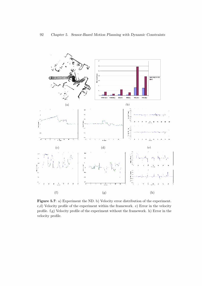
92 Chapter 5. Sensor-Based Motion Planning with Dynamic Constraints
(a) (b)
(c) (d) (e)
(f) (g) (h)
Figure 5.7: a) Experiment the ND. b) Velocity error distribution of the experiment.c,d) Velocity profile of the experiment within the framework. e) Error in the velocityprofile. f,g) Velocity profile of the experiment without the framework. h) Error in thevelocity profile.
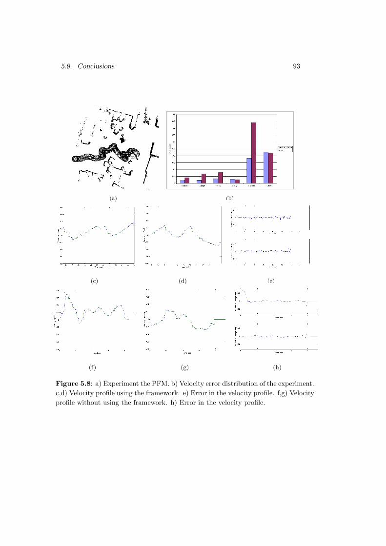
5.9. Conclusions 93
(a) (b)
(c) (d) (e)
(f) (g) (h)
Figure 5.8: a) Experiment the PFM. b) Velocity error distribution of the experiment.c,d) Velocity profile using the framework. e) Error in the velocity profile. f,g) Velocityprofile without using the framework. h) Error in the velocity profile.

94 Chapter 5. Sensor-Based Motion Planning with Dynamic Constraints
Chapter 6
The Sensor-Based NavigationSystem
6.1 Introduction
The Robotic community is building robots to accomplish tasks that requiremotion in human environments. ”Unfortunately”, the human environmentsare designed for humans, and the robot algorithms must adapt to these workplaces. The robots then deal with any shape unknown obstacles randomlyplaced in the environment. Moreover, the robot motion algorithms face an-other difficulty in these environments: they are full of humans that also move.Sharing the environment with humans, converts the work place in a highlydynamic scenario. Besides, the robot must also preserve the human safety(avoiding collisions with humans!). Fig. 6.1 illustrates an scenario of suchcharacteristics. The motion in these environments is a challenge for Robotics,but required for many mobile applications. This problem is dealt with in thisChapter: moving a robot in human-made scenarios that it is highly dynamic.
The Chapter firstly analyses the sensor-based navigation requirements thatmust be considered in order to navigate in the suggested scenarios. The com-pliance with the requirements mainly determines the success of the navigationtask, thus they all must be considered in the sensor-based navigation design.The proposed sensor-based navigation system is made up of three modules: amapping module, a planning module, and a reactive navigation method. Theyall cooperate to complete the collision avoidance task: (1) the mapping mod-ule deals with the sensory process, and thus with the environment nature -the module is designed to model unknown, highly dynamic, unstructured, andnon-predictable scenarios. (2) The planning module extracts the workspace
95
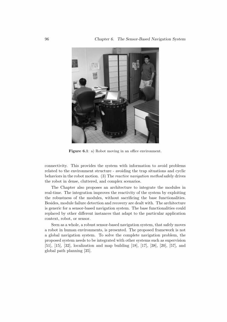
96 Chapter 6. The Sensor-Based Navigation System
Figure 6.1: a) Robot moving in an office environment.
connectivity. This provides the system with information to avoid problemsrelated to the environment structure - avoiding the trap situations and cyclicbehaviors in the robot motion. (3) The reactive navigation method safely drivesthe robot in dense, cluttered, and complex scenarios.
The Chapter also proposes an architecture to integrate the modules inreal-time. The integration improves the reactivity of the system by exploitingthe robustness of the modules, without sacrificing the base functionalities.Besides, module failure detection and recovery are dealt with. The architectureis generic for a sensor-based navigation system. The base functionalities couldreplaced by other different instances that adapt to the particular applicationcontext, robot, or sensor.
Seen as a whole, a robust sensor-based navigation system, that safely movesa robot in human environments, is presented. The proposed framework is nota global navigation system. To solve the complete navigation problem, theproposed system needs to be integrated with other systems such as supervision[51], [15], [32], localization and map building [18], [17], [38], [20], [57], andglobal path planning [35].
6.2. Navigation System Requirements 97
This research was previously presented in [48].The Chapter is organized as follows: The system requirements are intro-
duced in Section 6.2, and discussed in relation to related work in Section 6.3.Section 6.4 presents the three module-functionalities design. Section 6.5 in-troduces the complete navigation system. Section 6.7 discusses the frameworkand in Section 6.8 the conclusions are drawn.
6.2 Navigation System Requirements
The aim of this work is to develop a sensor-based navigation system to safelydrive a robot among locations in any human scenario. For this reason, therequirements that the environment nature and structure impose upon thenavigation system design are next summarized:
1. Robust reactive navigation: the motion commands have to be ro-bustly computed for a sensor-based motion planner. The reactive algo-rithm has to solve highly complex navigation problems: to successfullynavigate in very dense, complex, and cluttered scenarios.
2. Information integration: past sensory perceptions have to be inte-grated into a representation of the environment. Two reasons justifythis: (1) it gives a framework to have an incremental global reasoning.(2) Information of the past perceptions must be used to avoid obstaclesnot perceived at the current moment (visibility sensor constraints).
3. Reaction in dynamic environments: when the environment changesdynamically in a non-predictable way, the environmental representationhas to model rapidly the change. Otherwise, the robot will avoid partsof the space known to be free of obstacles, or will not avoid perceivedobstacles.
4. Trap situations and cyclic behaviors avoidance: There are manyobstacle configurations that produce trap situations, common for all thereactive navigation methods. The most typical are the U-shape obsta-cles. Moreover, there are some symmetric obstacle distributions wherethe reactive methods can produce alternated solutions. These environ-ments create cyclic behaviors in the robot motion. The robot will neverreach the goal location in both cases, unless a key is supplied.
5. Functionalities integration: The functionalities designed need to beintegrated within an architecture. Otherwise, interactions among func-
98 Chapter 6. The Sensor-Based Navigation System
tionalities must be designed from scratch to allow module replacement- portability among different platforms/sensors. Therefore, the modulecoordination requires failure detection and recovery.
The goal of this Chapter is to present a sensor-based navigation systemdesigned to comply with the above five requirements.
6.3 Related Work
This Section presents related work about sensor-based navigation systems.The discussion is directed towards the five requirements presented: robustreactive navigation, information integration, dynamic environments reaction,trap situations and cyclic behaviors avoidance, and functionalities integration.
Many sensor-based motion planners have been developed in the last years.Some of them use a physical analogy to compute motion commands [30], [34],[58], [9], [50]. Particular solutions to the inherent problems of these methods[33], f.e. [19], still appear in the literature. Other methods first compute somesets of motion commands. Next, a navigation strategy selects one motioncommand of these sets [22], [28], [56], [25]. Or there are methods that calculatesome form of high-level information description from the sensory information.Then, a motion command is computed, as opposed to being selected from apre-calculated set [54], [14]. The limitation of these methods is to robustlynavigate in complex, dense, and cluttered scenarios. These scenarios presenta high degree of difficulty for many existing sensor-based motion planners.
[14] is a framework that uses a path computed by a path planning algo-rithm. Incremental adjustments of the path are based on the sensory data,while maintaining the path in the free space. Some strategies were introducedto deal with dynamic environments: (1) letting an obstacle to jump overthe path, and (2) maintaining a set of alternative routes for selection. Trapsituations are avoided since a global path is always used. The difficulties ofthis method are to deal with situations where the path does not exist anymore,and to achieve robust navigation in dense, complex, and cluttered scenarios,see [12].
[59] uses an occupancy-grid of the environment, [10], to integrate theinformation. The reactive method uses the obstacle information of the localmap to compute safe motion commands. In highly dynamic environments,the method presents the difficulty of the sensors used, ultrasounds. Recently,[60] was presented. The trap situations are avoided by running the reactivealgorithm some steps before the algorithm execution. This method obtains
6.4. The Module-Functionalities Design 99
good results even running on platforms with low computational capabilities:the sensory integration is computationally efficient, and even with a reducednumber of steps local trap situations are avoided. However, the convergenceto the goal location depends on the number of steps selected. [11], [59], and[60] have the difficulty to achieve robust navigation when switching betweendense and less dense scenarios, see [59].
[13] is a sensor-based navigation system that formulates the problem asa constrained optimization in the velocity space. The cost function incorpo-rates global information to avoid the trap situations. The method uses aglobal-referred occupancy-grid that represents the robot configuration space.This local map is used to integrate the sensory information. The difficul-ties of this method are the computational load, and updating the free spacethat is indispensable in dynamic environments (the configuration space isrepresented in the grid).
The module integration is a point worth mentioning here. [59], [60] and[13] are sensor-based navigation systems that are made up of modules. How-ever, the module integration is not developed within any kind of architecture.
6.4 The Module-Functionalities Design
This Section presents the design of the modules that make up the sensor-basednavigation system. Firstly, the reactive algorithm base is discussed, Subsection6.4.1. Secondly, the design of the module dealing with the sensory process ispresented, Subsection 6.4.2. Finally, Subsection 6.4.3 introduces the modulethat allows for the trap situation avoidance.
6.4.1 Reactive Navigation Module
The reactive navigation method used is the Nearness Diagram Navigation,that is described in detail in Chapter 2. However, a brief description is nextpresented. The ND method is based on the situated-activity methodology ofdesign [3]. First, a set of five situations that fully describe the relative state ofthe robot, obstacle distribution, and goal location are defined. Subsequently,one action is designed for each situation. In real-time, the sensory informationis used to identify the current situation, and the associated action is executedcomputing the motion commands.
The reason for selecting the ND method is because it achieves robustnavigation. Good results in very dense, complex, and cluttered scenarios
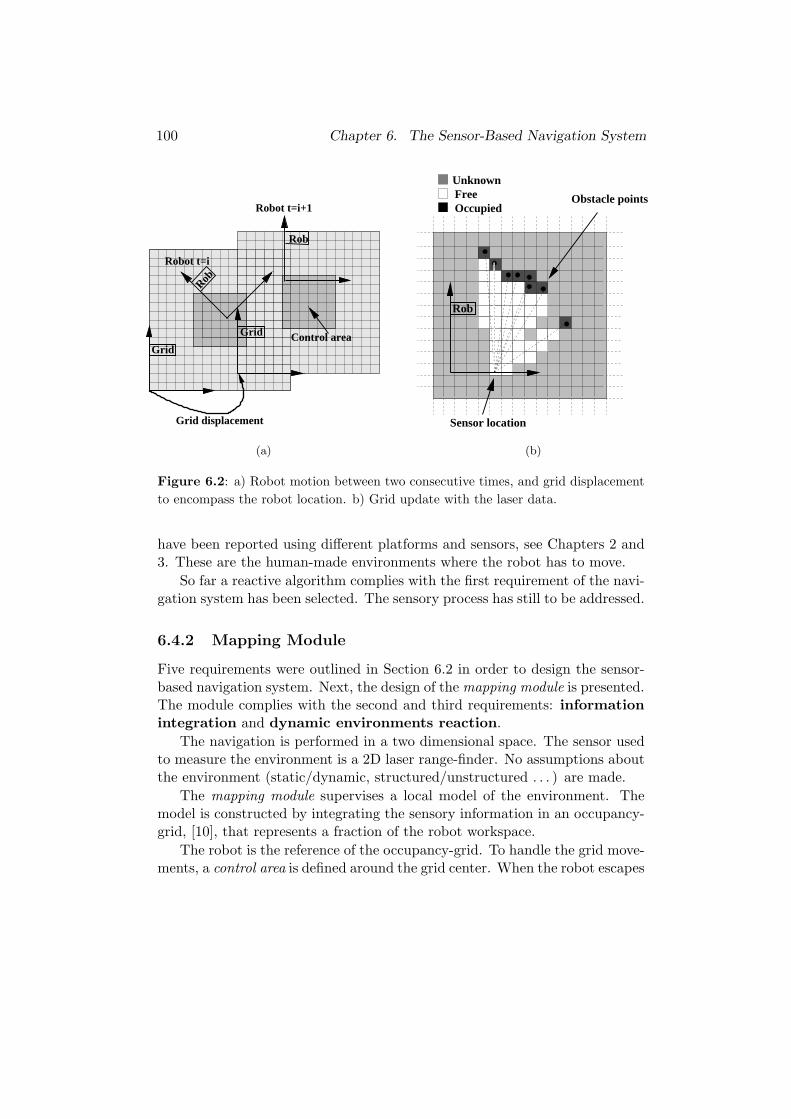
100 Chapter 6. The Sensor-Based Navigation System
Control area
Grid displacement
Robot t=i
Robot t=i+1Rob
Grid
Rob
Grid
FreeOccupied
Unknown
Obstacle points
Sensor location
Rob
(a) (b)
Figure 6.2: a) Robot motion between two consecutive times, and grid displacementto encompass the robot location. b) Grid update with the laser data.
have been reported using different platforms and sensors, see Chapters 2 and3. These are the human-made environments where the robot has to move.
So far a reactive algorithm complies with the first requirement of the navi-gation system has been selected. The sensory process has still to be addressed.
6.4.2 Mapping Module
Five requirements were outlined in Section 6.2 in order to design the sensor-based navigation system. Next, the design of the mapping module is presented.The module complies with the second and third requirements: informationintegration and dynamic environments reaction.
The navigation is performed in a two dimensional space. The sensor usedto measure the environment is a 2D laser range-finder. No assumptions aboutthe environment (static/dynamic, structured/unstructured . . . ) are made.
The mapping module supervises a local model of the environment. Themodel is constructed by integrating the sensory information in an occupancy-grid, [10], that represents a fraction of the robot workspace.
The robot is the reference of the occupancy-grid. To handle the grid move-ments, a control area is defined around the grid center. When the robot escapes
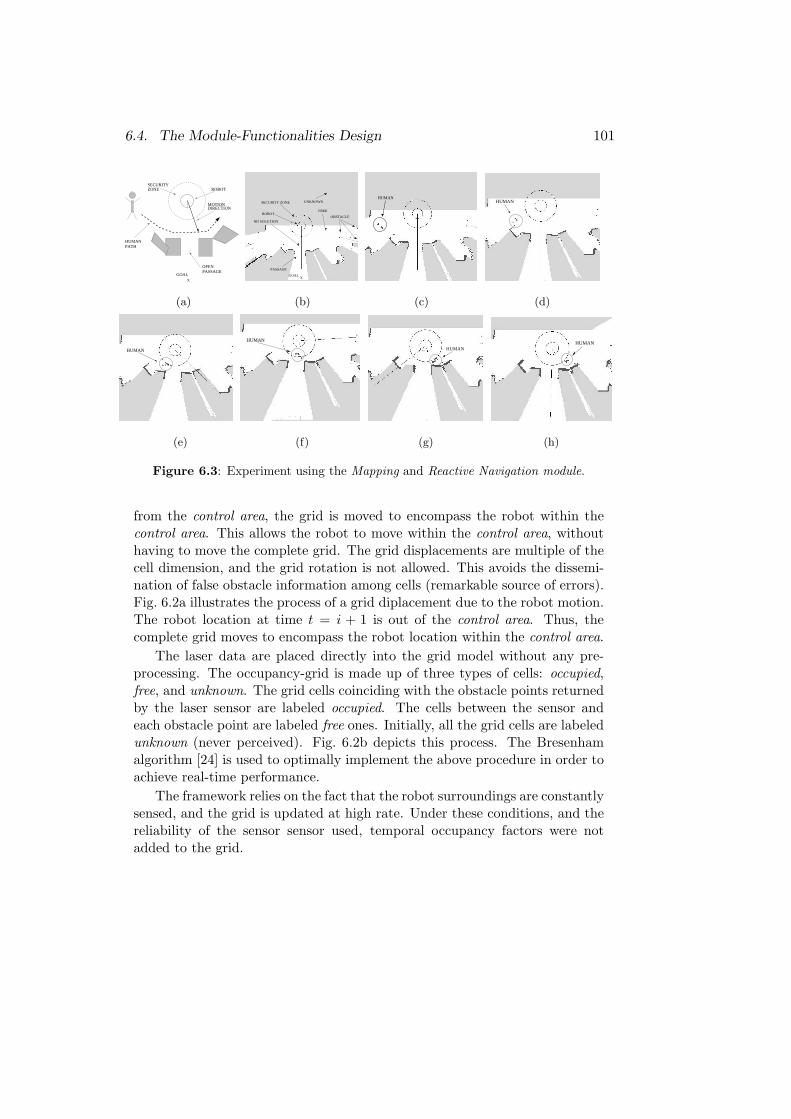
6.4. The Module-Functionalities Design 101
GOAL X
SECURITYZONE
MOTIONDIRECTION
HUMAN PATH
OPENPASSAGE
ROBOT
OBSTACLE
FREE
UNKNOWNSECURITY ZONE
ROBOT
XGOAL
PASSAGE
ND SOLUTION
HUMANHUMAN
(a) (b) (c) (d)
HUMAN
HUMAN
HUMANHUMAN
(e) (f) (g) (h)
Figure 6.3: Experiment using the Mapping and Reactive Navigation module.
from the control area, the grid is moved to encompass the robot within thecontrol area. This allows the robot to move within the control area, withouthaving to move the complete grid. The grid displacements are multiple of thecell dimension, and the grid rotation is not allowed. This avoids the dissemi-nation of false obstacle information among cells (remarkable source of errors).Fig. 6.2a illustrates the process of a grid diplacement due to the robot motion.The robot location at time t = i + 1 is out of the control area. Thus, thecomplete grid moves to encompass the robot location within the control area.
The laser data are placed directly into the grid model without any pre-processing. The occupancy-grid is made up of three types of cells: occupied,free, and unknown. The grid cells coinciding with the obstacle points returnedby the laser sensor are labeled occupied. The cells between the sensor andeach obstacle point are labeled free ones. Initially, all the grid cells are labeledunknown (never perceived). Fig. 6.2b depicts this process. The Bresenhamalgorithm [24] is used to optimally implement the above procedure in order toachieve real-time performance.
The framework relies on the fact that the robot surroundings are constantlysensed, and the grid is updated at high rate. Under these conditions, and thereliability of the sensor sensor used, temporal occupancy factors were notadded to the grid.
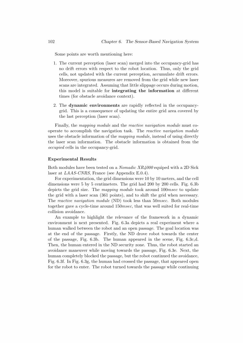
102 Chapter 6. The Sensor-Based Navigation System
Some points are worth mentioning here:
1. The current perception (laser scan) merged into the occupancy-grid hasno drift errors with respect to the robot location. Thus, only the gridcells, not updated with the current perception, accumulate drift errors.Moreover, spurious measures are removed from the grid while new laserscans are integrated. Assuming that little slippage occurs during motion,this model is suitable for integrating the information at differenttimes (for obstacle avoidance context).
2. The dynamic environments are rapidly reflected in the occupancy-grid. This is a consequence of updating the entire grid area covered bythe last perception (laser scan).
Finally, the mapping module and the reactive navigation module must co-operate to accomplish the navigation task. The reactive navigation moduleuses the obstacle information of the mapping module, instead of using directlythe laser scan information. The obstacle information is obtained from theoccupied cells in the occupancy-grid.
Experimental Results
Both modules have been tested on a Nomadic XR4000 equiped with a 2D Sicklaser at LAAS-CNRS, France (see Appendix E.0.4).
For experimentation, the grid dimensions were 10 by 10 meters, and the celldimensions were 5 by 5 centimeters. The grid had 200 by 200 cells. Fig. 6.3bdepicts the grid size. The mapping module took around 100msec to updatethe grid with a laser scan (361 points), and to shift the grid when necessary.The reactive navigation module (ND) took less than 50msec. Both modulestogether gave a cycle-time around 150msec, that was well suited for real-timecollision avoidance.
An example to highlight the relevance of the framework in a dynamicenvironment is next presented. Fig. 6.3a depicts a real experiment where ahuman walked between the robot and an open passage. The goal location wasat the end of the passage. Firstly, the ND drove robot towards the centerof the passage, Fig. 6.3b. The human appeared in the scene, Fig. 6.3c,d.Then, the human entered in the ND security zone. Thus, the robot started anavoidance maneuver while moving towards the passage, Fig. 6.3e. Next, thehuman completely blocked the passage, but the robot continued the avoidance,Fig. 6.3f. In Fig. 6.3g, the human had crossed the passage, that appeared openfor the robot to enter. The robot turned towards the passage while continuing
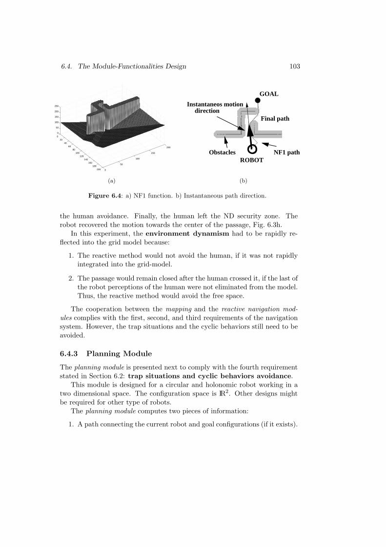
6.4. The Module-Functionalities Design 103
020
4060
80100
120140
160180
200 0
50
100
150
200
0
50
100
150
200
250
x
direction
GOAL
NF1 pathROBOT
Final path
Obstacles
Instantaneos motion
(a) (b)
Figure 6.4: a) NF1 function. b) Instantaneous path direction.
the human avoidance. Finally, the human left the ND security zone. Therobot recovered the motion towards the center of the passage, Fig. 6.3h.
In this experiment, the environment dynamism had to be rapidly re-flected into the grid model because:
1. The reactive method would not avoid the human, if it was not rapidlyintegrated into the grid-model.
2. The passage would remain closed after the human crossed it, if the last ofthe robot perceptions of the human were not eliminated from the model.Thus, the reactive method would avoid the free space.
The cooperation between the mapping and the reactive navigation mod-ules complies with the first, second, and third requirements of the navigationsystem. However, the trap situations and the cyclic behaviors still need to beavoided.
6.4.3 Planning Module
The planning module is presented next to comply with the fourth requirementstated in Section 6.2: trap situations and cyclic behaviors avoidance.
This module is designed for a circular and holonomic robot working in atwo dimensional space. The configuration space is IR2. Other designs mightbe required for other type of robots.
The planning module computes two pieces of information:
1. A path connecting the current robot and goal configurations (if it exists).
104 Chapter 6. The Sensor-Based Navigation System
PATH
INSTANTANEOUSPATH DIRECTION
X GOAL
ND SOLUTION
ROBOT
(a) (b) (c) (d)INSTANTANEOUSPATH DIRECTION
XGOAL
PATH
PASSAGECLOSED
(e) (f) (g) (h)
Figure 6.5: Experiment using the Mapping, planning, and reactive navigation md-dules.
2. The instantaneous path direction in order to reach the goal configuration.This direction is the main direction of the first part of the path.
The next procedure is followed to compute the path: (1) the obstacle infor-mation in the occupancy-grid is used to compute the C-Obstacles (by enlargingthe obstacles with the robot radius), see Fig. 6.4b. (2) The Navigation Func-tion 11 [35] is constructed over the grid2 (see Fig. 6.4a). (3) A collision-freepath, connecting the current robot configuration and the goal configuration,is obtained by a gradient-search technique over the NF1. (4) The path is”stretched” with a recursive algorithm to be optimized, see Fig. 6.4b. This”stretch” strategy avoids the border effects of the NF1 function, and it modi-fies paths pointing towards or skirting the obstacles. The reasons for selectionof this path planning algorithm are: (1) the NF1 is a minima-free naviga-
1The Navigation Function 1 (NF1) is a potential built over a grid representation of theconfiguration space. A wave is propagated among the free cells from the goal cell to all thefree cells in the grid. The free cells are labeled with the minimum number of cells crossed toreach the goal location.
2The free space assumption is considered here. That is, the unknown space is consideredfree for the NF1 function computation.
6.4. The Module-Functionalities Design 105
tion function. (2) The NF1 is a grid-based navigation function, compatiblewith the grid-model available. (3) The path planning algorithm is simple andefficient, then it can be used at each sampling time.
The assumption here is that a path exists. When a path is not availablethis module produces a failure. This will be supervised by the complete systempresented in the next Section.
The three modules work together as follows. The mapping module con-structs the occupancy-grid. The planning module uses the occupancy-grid tocompute the instantaneous path direction. The reactive navigation methoduses the obstacle information in the occupancy-grid, and the instantaneouspath direction, to compute the motion commands.
Experimental Results
For experimentation, the same robot and settings presented in Subsection 6.4.2were used. The first meter of the path was used to compute the instantaneouspath direction. The planning module imposed an additional time penalty of100msec. The cycle time then was 250msec, enough for real-time.
An experiment to highlight the relevance of this framework in trap sit-uations is presented next. Fig. 6.5a depict the initial state, that match upwith Fig. 6.8e. Figs. 6.5b,c,d illustrates the robot navigating along a passagein order to reach the final location. While the robot was traveling, a humanblocked the end, see Fig. 6.8f. The environmental structure was modified, anda big U-shape obstacle was created. This produced a trap situation for therobot, see Fig. 6.5e. Rapidly, the mapping module reflected the change, andthe planning module calculated a new path. The instantaneous path directionpointed away from the U-shape configuration, see Fig. 6.5e. The ND computedthe motion commands to follow this direction, see Figs. 6.5f,g,h. Therefore,the robot was driven out of the U-shape obstacle. The trap situation wasavoided, see Fig. 6.8g.
The reactive method, mapping module, and planning module working to-gether avoid trap situations and cyclic behaviors:
• There are no obstacle configurations that produce trap situations(when a solution exists within the grid-model). The instantaneous pathdirection is used to get the robot out of these situations.
• Any symmetry of the environment does not produce cyclic behaviorsin the robot motion. The possible symmetrical motions are discriminatedby the instantaneous path direction.
106 Chapter 6. The Sensor-Based Navigation System
This framework complies with the first four requirements. The completesensor-based navigation system is presented next.
6.5 The Sensor-Based Navigation System
This Section addresses the integration of the functionalities, the fifthrequirement. An architecture is proposed that specifies the interactions amongthe modules. Moreover, failures in the planning module and in the reactivemethod are dealt with.
Planning module failure. There exist two cases where a planning algo-rithm cannot find a path, connecting the robot and goal configurations:
1. The goal configuration is not in free space Cfree [35] (final configurationin collision with an obstacle). This is a typical situation in unknownscenarios, where goals are randomly placed for exploration. While thescenario is progressively perceived, the goal can be within an obstacle.In dynamic scenarios an object can move, or even stop, over the goallocation. Even in static and known environments, this situation appearswhen the goal moves within an obstacle due to the robot drift.
2. The robot or the goal are surrounded by an obstacle.
Notice that both situations can appear irrespectively of the distance tothe goal location. These situations could be avoided by replacing the goallocation. However, the role of the navigation system is not to modify the goallocation (imposed by an external agent). The consequences can drasticallydetermine the success of the global task.
The planning module produces a failure in these situations. However, thesystem must be able to continue the navigation task (close the motion controlloop).
Reactive navigation failure. The ND method uses an internal pieceof information named free walking area (in short, it represents a region todrive the robot). If there is not free walking area available, the goal cannot bereached. This situation appears when the robot is completely surrounded byobstacles. The reactive method produces a failure in this situation.
The following architecture specifies the module interaction and deals withmodule failures, see Fig. 6.6. The navigation system works as follows:
Procedure Navigation System step (n, goal)Datalaser = Read Laser
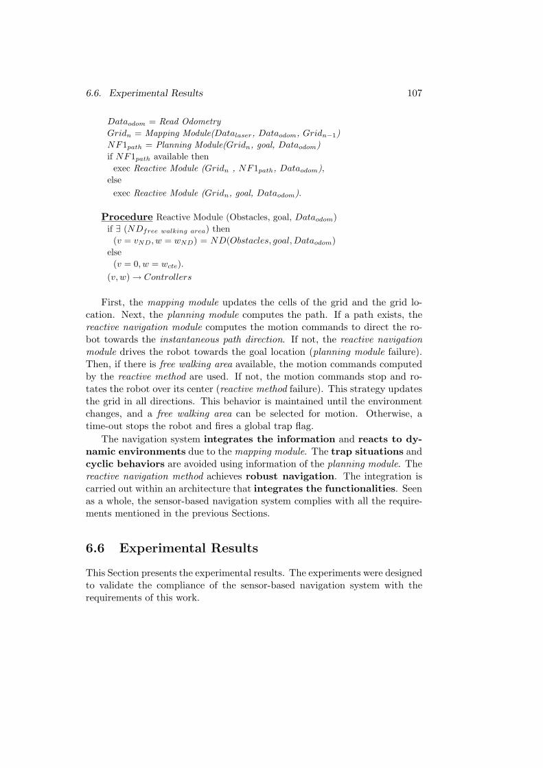
6.6. Experimental Results 107
Dataodom = Read OdometryGridn = Mapping Module(Datalaser, Dataodom, Gridn−1)NF1path = Planning Module(Gridn, goal, Dataodom)if NF1path available then
exec Reactive Module (Gridn , NF1path, Dataodom),else
exec Reactive Module (Gridn, goal, Dataodom).
Procedure Reactive Module (Obstacles, goal, Dataodom)if ∃ (NDfree walking area) then
(v = vND, w = wND) = ND(Obstacles, goal, Dataodom)else
(v = 0, w = wcte).(v, w) → Controllers
First, the mapping module updates the cells of the grid and the grid lo-cation. Next, the planning module computes the path. If a path exists, thereactive navigation module computes the motion commands to direct the ro-bot towards the instantaneous path direction. If not, the reactive navigationmodule drives the robot towards the goal location (planning module failure).Then, if there is free walking area available, the motion commands computedby the reactive method are used. If not, the motion commands stop and ro-tates the robot over its center (reactive method failure). This strategy updatesthe grid in all directions. This behavior is maintained until the environmentchanges, and a free walking area can be selected for motion. Otherwise, atime-out stops the robot and fires a global trap flag.
The navigation system integrates the information and reacts to dy-namic environments due to the mapping module. The trap situations andcyclic behaviors are avoided using information of the planning module. Thereactive navigation method achieves robust navigation. The integration iscarried out within an architecture that integrates the functionalities. Seenas a whole, the sensor-based navigation system complies with all the require-ments mentioned in the previous Sections.
6.6 Experimental Results
This Section presents the experimental results. The experiments were designedto validate the compliance of the sensor-based navigation system with therequirements of this work.
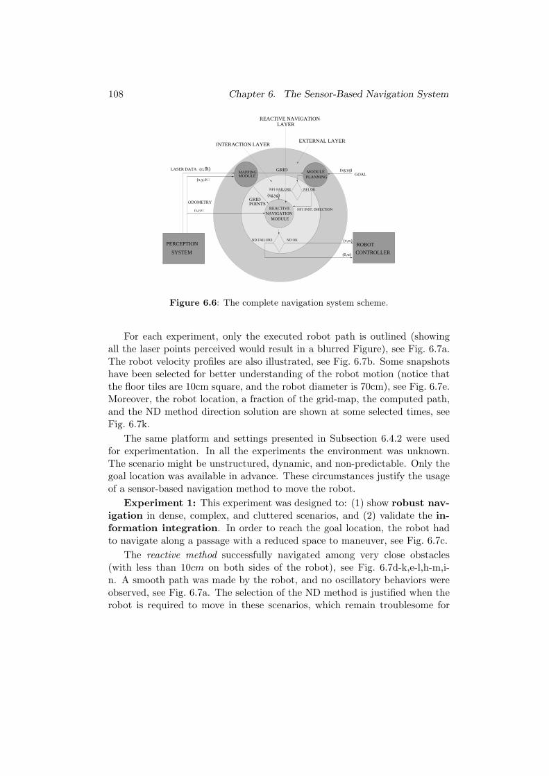
108 Chapter 6. The Sensor-Based Navigation System
(x,y,ϑ)
PERCEPTION
SYSTEM
GOALϑ
ϑ)
(v,w)
(xg,yg)GRID
(xg,yg)
(x,y,
(ri, i)
CONTROLLER
ROBOT
GRIDPOINTS
MODULEPLANNINGMODULE
MAPPING
EXTERNAL LAYERINTERACTION LAYER
REACTIVE NAVIGATIONLAYER
LASER DATA
ODOMETRY
NF1 OK
NF1 INST. DIRECTION
NF1 FAILURE
ND OKND FAILURE
(0,w)
REACTIVE NAVIGATION
MODULE
Figure 6.6: The complete navigation system scheme.
For each experiment, only the executed robot path is outlined (showingall the laser points perceived would result in a blurred Figure), see Fig. 6.7a.The robot velocity profiles are also illustrated, see Fig. 6.7b. Some snapshotshave been selected for better understanding of the robot motion (notice thatthe floor tiles are 10cm square, and the robot diameter is 70cm), see Fig. 6.7e.Moreover, the robot location, a fraction of the grid-map, the computed path,and the ND method direction solution are shown at some selected times, seeFig. 6.7k.
The same platform and settings presented in Subsection 6.4.2 were usedfor experimentation. In all the experiments the environment was unknown.The scenario might be unstructured, dynamic, and non-predictable. Only thegoal location was available in advance. These circumstances justify the usageof a sensor-based navigation method to move the robot.
Experiment 1: This experiment was designed to: (1) show robust nav-igation in dense, complex, and cluttered scenarios, and (2) validate the in-formation integration. In order to reach the goal location, the robot hadto navigate along a passage with a reduced space to maneuver, see Fig. 6.7c.
The reactive method successfully navigated among very close obstacles(with less than 10cm on both sides of the robot), see Fig. 6.7d-k,e-l,h-m,i-n. A smooth path was made by the robot, and no oscillatory behaviors wereobserved, see Fig. 6.7a. The selection of the ND method is justified when therobot is required to move in these scenarios, which remain troublesome for
6.6. Experimental Results 109
other existing reactive methods. A deep discussion about navigation in thesescenarios is presented in [44].
The mapping module also played an important role because:
• New sensory perceptions were rapidly integrated into the grid. Thus,the robot avoided the new obstacles when they were perceived, see thesequence of Figs. 6.7k,l,m,n.
• Past sensory perceptions remained integrated into the grid. Due to thesensor visibility constraints and its location within the robot3, some-times the closest obstacles were not perceived. Figs. 6.7g,h-m,i-n depictmoments when this happened. However, these obstacles were perceivedsome time before, thus, they remained in the grid and collisions wereavoided.
The velocity profile is illustrated in Fig. 6.7b. The robot moved at lowspeeds due to the complexity of the scenario. The maximum speed wasachieved when the robot was out of the passage. The time of the experimentwas 127sec, and the average translational velocity was 0.204 m
sec .Experiment 2: This experiment was designed to test the trap situ-
ations avoidance. Fig. 6.8c shows the initial state of the robot and theenvironment. The robot must navigate along the passage to reach the goallocation. Three consecutive trap situations were produced by changes in theenvironment structure.
The robot started by navigating along the passage, Fig. 6.8d-k. Whilethe robot was moving forward, a passage on the rigth-hand was opened (therobot could not perceive it), see Fig. 6.8d,e. Reaching the end of the passage,a human placed a box closing the main way, see Fig. 6.8f-l. The robot wastrapped within a big U-shape obstacle. Due to the information provided bythe planning module, computed from the environmental model kept by themapping module, the robot rapidly turned and move backwards in the passageto avoid the trap situation. This part of the experiment is displayed step bystep in Fig. 6.5. The robot perceived the open passage on the right-hand whilenavigating to get out of the passage. The new passage was rapidly integratedinto the grid. Then, the robot moved towards the new passage, see Fig. 6.8g.Then, the human closed the new passage, see Fig. 6.8h-m. The change wasrapidly modeled, and the robot was driven out of the passage, avoiding thenew trap situation, see Fig. 6.8i-n. Finally, the global trap situation was
3Notice that the sensor is placed 0.24cm away from the center of the robot. The sensorhas a 180◦ field of visibility.
110 Chapter 6. The Sensor-Based Navigation System
avoided, see Fig. 6.8j, and the robot resumed the motion towards the goallocation.
The path made by the robot is shown in Fig. 6.8a. The velocity profilesare illustrated Fig. 6.8b (only 150sec due to a memory limitation). The com-plete time of the task was 200sec, and the average translational velocity was0.233 m
sec .Experiment 3: This experiment shows the robot navigating in a typical
populated and changing scenario. The sensor-based navigation system mustcomply with all the requirements proposed in order to successfully navigate inthis scenario. Fig. 6.9c depicts the initial state of the robot and the environ-ment. The robot had to cross the hall to reach the final location.
During the first part of the experiment humans were randomly walking,building, and modifying the environment to hinder the robot motion, seeFig. 6.9c,d,e,f. In this part of the experiment the mapping module was rapidlyreflecting the environmental changes. Then, the reactive method was suc-cessfully avoiding collisions. Notice that, if the sensory information were notproperly integrated, a barrier of obstacles would appear in the grid. Thus,the robot would not be able to avoid the collisions, or would avoid the freespace. Subsequently, the humans built an obstacle configuration that trappedthe robot, see Fig. 6.9g. The planning module rapidly provided informationused by the reactive method to drive the robot out to the U-shape obstacle,see Fig. 6.9h. Finally, the robot resumed the motion and reached the goallocation while reacting to the human motion, see Fig. 6.9i,j.
Unfortunately the information of the experiment was lost. However, avery similar run is discussed. The highly dynamic nature of the environmentis depicted in Fig. 6.9k,l. They could be compared with the Fig. 6.9c,d,e,f.Subsequently, the humans produced a trap situation, see Fig. 6.9m, similar tothe Fig. 6.9g. The robot turned to the right to avoid the trap situation. Finally,the robot continued the motion in an environment continuously changing, seeFig. 6.9n.
The path executed by the robot is shown in Fig. 6.9a. The velocity profile isillustrated Fig. 6.9b (only 150sec due to a memory limitation). The completetime of the experiment was 170sec, and the average translational velocity was0.196 m
sec .
6.7 Discussion
The strength of the navigation system is the quality and robustness of thenavigation performance. The robot successfully navigates in troublesome sce-
6.7. Discussion 111
narios due to the compliance with the requirements presented in Section 6.2.These scenarios would produce difficulties to other existing methods, sincenone of them address all these requirements presented.
The limitation of the proposed sensor-based navigation system is the com-putational load (in our current implementation a Pentium II is used. To workon systems with low computational capabilities, the size of the grid map wouldbe reduced. This would affect the locality of the navigation method proposed.
The functional modularity and the coordination, both give generality,portability, robustness, and efficacy to the navigation system. To validatethis last statement, the navigation system was tested with some modificationson two indoor and one outdoor robot at LAAS-CNRS, France; on one indoorrobot at the Technical University of Lisbon, Portugal; and on an indoor robotat the University of Zaragoza, Spain. The reactive method ND was modifiedto work on robots with non-circular shapes and with kinematic constraints,see [45]. The mapping module was re-designed to work with a tri-dimensionallaser, and with ultrasounds [10]. For the outdoor robot an special module toprocess visual information was used [27]. In the planning module some changeswere required to take into account the specific robot characteristics. The newmodules were integrated within the architecture. Thus, the portability amongplatforms was straightforward.
The presented navigation system is not a complete navigation system. Thesystem internal model represents a local fraction of the environment (settingthe locality of the method). Then, the system relies on higher levels to ac-complish a global navigation task: supervision, global planning, localization,and map building. To date, the proposed navigation system has been used asthe sensor-based navigation system for a topological-based navigation [63]. Aglobal topological model of the environment is built on-line, while the robot isself-located within the model. From the model, sub-goals are placed for explo-ration, and they are reached by means of the presented sensor-based navigationsystem. Currently, in the Robels system [51], the navigation system is one ofthe five sensory-motor functions used to perform the robot motion. Moreover,the navigation system has been successfully integrated as the low-level motiongenerator in the complete GenoM architecture [23] on the Nomadic XR4000at LAAS-CNRS, France. The navigation system is daily used to move theplatform.
112 Chapter 6. The Sensor-Based Navigation System
6.8 Conclusions
In this Chapter a sensor-based navigation system for collision avoidance inhuman-made scenarios has presented. Five navigation requirements were iden-tified in order to navigate in these scenarios: robust navigation, informationintegration, reaction in dynamic environments, trap situations and cyclic be-haviors avoidance, and functionalities integration. The navigation systemcompliance with these requirements has been the main design requirement.The consequence is a sensor-based navigation system that achieves robustnavigation in dense, complex, cluttered, unknown, and highly dynamic sce-narios. Besides, the trap situations and cyclic behaviors in the robot motionare avoided. This is illustrated in the experimental results. Moreover, thenavigation system is validated by the robots that everyday make use of it.
The architecture that embeeds the funtionalities allows for module replace-ment, and for module failure and recovery. The function modularity and thearchitecture, both are the basis for the integration of the research, presentedin previous Chapters, in a unique framework. Besides, this navigation systemis the basis for the development of a complete navigation system.
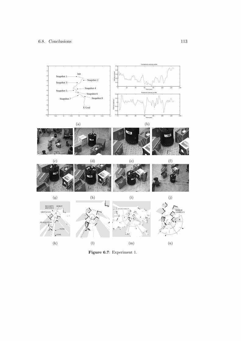
6.8. Conclusions 113
−5 −4.5 −4 −3.5 −3 −2.5 −2 −1.5 −1−10
−9
−8
−7
−6
−5
−4
−3
−2
−1
0
Snapshot 1
Snapshot 2Snapshot 3
Snapshot 4Snapshot 5
Snapshot 6
Snapshot 7
X Goal
Init
Snapshot 8
0 20 40 60 80 100 120 1400
0.1
0.2
0.3
0.4
0.5Tranlational velocity profile
Time (sec)
Vel
ocity
(m
/sec
)0 20 40 60 80 100 120 140
−0.3
−0.2
−0.1
0
0.1
0.2Rotational velocity profile
Time (sec)
Vel
ocity
(ra
d/se
c)
(a) (b)
XGOAL
(c) (d) (e) (f)
(g) (h) (i) (j)
GOAL
ROBOTSECURITY DISTANCE
OBSTACLES
PATH
ND SOLUTION
SENSOR VISIBILITYSENSORVISIBILITY
(k) (l) (m) (n)
Figure 6.7: Experiment 1.
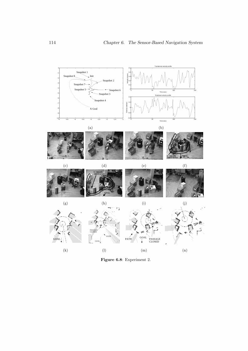
114 Chapter 6. The Sensor-Based Navigation System
−5 −4.5 −4 −3.5 −3 −2.5 −2 −1.5 −1−10
−9
−8
−7
−6
−5
−4
−3
−2
−1
0
Init
X Goal
Snapshot 1
Snapshot 6
Snapshot 8
Snapshot 7
Snapshot 5
Snapshot 2
Snapshot 3
Snapshot 4
0 50 100 1500
0.1
0.2
0.3
0.4
0.5Tranlational velocity profile
Time (sec)
Vel
ocity
(m
/sec
)
0 50 100 150−0.4
−0.2
0
0.2
0.4Rotational velocity profile
Time (sec)
Vel
ocity
(ra
d/se
c)(a) (b)
XGOAL
OBSTACLEU−SHAPE GOAL
(c) (d) (e) (f)
U−SHAPE
OBSTACLE
GOAL
(g) (h) (i) (j)
GOALX
PASSAGECLOSED
PATH
GOALPATH
GOALPASSAGECLOSED
(k) (l) (m) (n)
Figure 6.8: Experiment 2.
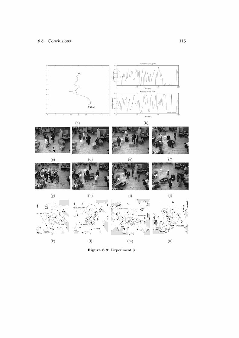
6.8. Conclusions 115
−5 −4.5 −4 −3.5 −3 −2.5 −2 −1.5 −1−10
−9
−8
−7
−6
−5
−4
−3
−2
−1
0
Init
X Goal
0 50 100 1500
0.1
0.2
0.3
0.4
0.5Tranlational velocity profile
Time (sec)
Vel
ocity
(m
/sec
)0 50 100 150
−0.4
−0.2
0
0.2
0.4Rotational velocity profile
Time (sec)
Vel
ocity
(ra
d/se
c)
(a) (b)
GOAL
(c) (d) (e) (f)
U−SHAPE
OBSTACLE
GOAL
X
(g) (h) (i) (j)
GOALX
PATH
ND SOLUTION
HUMANS
XGOAL
HUMANS
PATH
ND SOLUTION
GOAL
X
ND SOLUTION
HUMANS
U−SHAPE OBSTACLE
PATH
HUMANS
GOALX
PATH
(k) (l) (m) (n)
Figure 6.9: Experiment 3.

116 Chapter 6. The Sensor-Based Navigation System
Chapter 7
Conclusions
The work presented in this memory contributes to the sensor-based motionplanning field. Each chapter has a different nature, and addresses a differenttopic in this field. The main contributions are:
• Sensor-based motion planning
Chapter 2 addresses the sensor-based motion planning by presenting thedesign of a reactive navigation method.
The reactive navigation method has been designed using the situated-activity paradigm of behavioral design. By using this paradigm, thereactive navigation problem is broken down into sub-problems. Thisstrategy simplifies the complete reactive navigation problem. As a con-sequence, a new method implementation of the proposed design leadsto a new reactive navigation method. The new method might success-fully move a robot in more troublesome scenarios than other methodsdo. That is, the robot might be able to successfully navigate in dense,complex, and cluttered environments.
To demonstrate the utility of the design, a geometric implementationcalled Nearness Diagram Navigation has been presented. The methodhas been validated using a real platform. Up to date the author doesnot know any other method or approach that performs better navigationthan the Nearness Diagram Navigation.
• Under-constraint Sensor-based Motion Planning
The Chapter 3 presents and under-constrained solution to extend theNearness Diagram Navigation method, to work on robots with non-circular shapes considering the kinematics and dynamics. By using the
117
118 Chapter 7. Conclusions
proposed framework, constrained robots are successfully move in dense,complex, and cluttered scenarios.
Experimental results on five different robots using different sensors vali-date the utility, and easy portability, of this reactive navigation method.The author believes that this method is one of the most robust sensor-based motion planners to drive constrained robots in troublesome sce-narios.
• Sensor-based motion planning with kinematic constraints
To address the kinematic constraints, Chapter 4 presents the Ego-KinematicSpace. This space can be used to convert existing reactive navigationmethods that do not address the kinematic constraints in methods thatdo. A space, where the methods produce solutions that comply withthe kinematics, has been constructed. To validate this framework, tworeactive navigation methods have been successfully used to safely drive akinematic constrained platform among locations. Both methods do notaddress the kinematics. The author believes that this is a wide solutionto address the kinematics in sensor-based motion planning.
Another contribution of this Chapter is to demonstrate, that the sub-space that really matters for sensor-based motion planning with kine-matic constraints, is two-dimensional (instead of three-dimensional, asit has been classically addressed). The author believes that this resultwill alleviate significantly the computations required by new methods inthe future.
• Sensor-based motion planning with dynamic constraints
To address the dynamic constraints, Chapter 5 presents the Ego-DynamicSpace. This space is constructed by using the dynamic constraints. Thus,reactive methods used in this space compute solutions that comply withthe robot dynamics constraints. To validate the framework two reac-tive navigation methods have been successfully used to safely drive adynamic constrained platform among locations. Both methods do notaddress dynamics. The author believes that this is a wide solution toaddress the dynamic constraints into the sensor-based motion planningdiscipline.
• Sensor-based navigation system
This thesis also addresses the improvement of the behavior of reactivenavigation methods. Chapter 6 proposes an architecture to coordinate
119
some modules in order to improve the reactivity of the pure naviga-tion base algorithm. By means of the complete framework, the robotsuccessfully navigates in highly dynamic scenarios, while avoiding thewell-known trap situations. The proposed framework has been validatedwith a real platform.
Moreover, this Chapter is the basis for the integration of all the tech-nologies proposed in other Chapters in a unique framework.
To discuss the future work, consider the following two questions: (1) howmany mobile vehicles exists (earth, air, water, space, . . .)? (2) For which ofthem, safe motion is computed robustly? Consider shape, kinematics, dy-namics, sensors difficulties, different scenarios . . .. There are many problemsstill to be solved, at least in Sensor-Based Motion Planning, to develop appli-cations in the real world.

120 Chapter 7. Conclusions
Bibliography
[1] R. Alami, I. Belousov, S. Fleury, M.Herb, F. Ingrand, J. Minguez, andB. Morisset. Diligent: Towards a human-friendly navigation system. InIEEE-RSJ Int. Conf. on Intelligent Robots and Systems, pages 2094–2100,Takamatsu, Japan, 2000.
[2] J.C. Alvarez, A. Shkel, and V. Lumelsky. Building topological models fornavigation in large scale environments. In IEEE International Conferenceon Robotics and Automation, Leuven, Belgium, 1998.
[3] R.C. Arkin. Behavior-Based Robotics. The MIT Press, 1999.
[4] K. Arras, J. Persson, N. Tomatis, and R. Siegwart. Real-time ObstacleAvoidance for Polygonal Robots with a Reduced Dynamic Window. InIEEE Int. Conf. on Robotics and Automation, pages 3050–3055, Wash-ington, USA, 2002.
[5] J. Asensio and L. Montano. A Kinematic and Dynamic Model-BasedMotion Controller for Mobile Robots. In 15th IFAC World Congress,Barcelona, Spain, 2002.
[6] K. Azarm and G. Schmidt. Integrated mobile robot motion planning andexecution in changing indoor environments. In IEEE/RSJ InternationalConference on Intelligent Robots and Systems, pages 298–305, Munchen,Germany, 1994.
[7] J. Barraquand and J.C. Latombe. On nonholonomic mobile robots andoptimal maneuvering. In Intelligent Symposium on Intelligent Control,pages 340–346, Albany, 1989.
[8] J.D. Boissonnat and X.N. Xi. Accesibility region for a car that only moveforward along optimal paths. In Research Report INRIA 2181, Sophia-Antipolis, France, 1994.
121
122 BIBLIOGRAPHY
[9] J. Borenstein and Y. Koren. Real-Time Obstacle Avoidance for FastMobile Robots. IEEE Transactions on Systems, Man and Cybernetics,19(5):1179–1187, 1989.
[10] J. Borenstein and Y. Koren. Histogramic in-Motion Mapping for MobileRobot Obstacle Avoidance. IEEE Journal on Robotics and Automation,7(4):535–539, 1991.
[11] J. Borenstein and Y. Koren. The Vector Field Histogram–Fast Obsta-cle Avoidance for Mobile Robots. IEEE Transactions on Robotics andAutomation, 7:278–288, 1991.
[12] O. Brock. Generating Robot Motion: The Integration of Planning andExecution. PhD thesis, Stanford University, 1999.
[13] O. Brock and O. Khatib. High-Speed Navigation Using the Global Dy-namic Window Approach. In IEEE Int. Conf. on Robotics and Automa-tion, pages 341–346, Detroit, MI, 1999.
[14] O. Brock and O. Khatib. Real-Time Replanning in High-DimensionalConfiguration Spaces using Sets of Homotopic Paths. In IEEE Int. Conf.on Robotics and Automation, pages 550–555, San Francisco, USA, 2000.
[15] Joachim M. Buhmann, Wolfram Burgard, Armin B. Cremers, Dieter Fox,Thomas Hofmann, Frank E. Schneider, Jiannis Strikos, and SebastianThrun. The mobile robot RHINO. AI Magazine, 16(2):31–38, 1995.
[16] A. Calcitti and R. Zapata. Reactive Behaviours of Mobile Manipula-tors Based on the DWZ Approach. In IEEE Int. Conf. on Robotics andAutomation, Korea, 2001.
[17] J. A. Castellanos, J.M.M. Montiel, J. Neira, and J. D. Tardos. TheSPmap: A probabilistic framework for simultaneous localization and mapbuilding. IEEE Trans. Robotics and Automation, 15(5):948–952, 1999.
[18] J. A. Castellanos and J. D. Tardos. Mobile Robot Localization and MapBuilding: A Multisensor Fusion Approach. Kluwer Academic Publishers,Boston, 1999.
[19] L. Chenqing, M. Ang, H. Krishman, and L. Yong. Virtual Obstacle Con-cept for Local-minimum-recovery in Potential-field Based Navigation. InIEEE Int. Conf. on Robotics and Automation, pages 983–989, San Fran-cisco, USA, 2000.
BIBLIOGRAPHY 123
[20] M. W. M. G. Dissanayake, P. Newman, H. F. Durrant-Whyte, S. Clark,and M. Csorba. A solution to the simultaneous localization andmap building (slam) problem. IEEE Trans. Robotics and Automation,17(3):229–241, 2001.
[21] L.E Dubins. On curves of minimal lenght with a constraint on averagecurvature and with prescribed initial and terminal positions and tangents.Amer. J. Math., 57:497–516, 1957.
[22] W. Feiten, R. Bauer, and G. Lawitzky. Robust Obstacle Avoidance inUnknown and Cramped Environments. In IEEE Int. Conf. on Roboticsand Automation, pages 2412–2417, San Diego, USA, 1994.
[23] S. Fleury. Architecture de controle distribuee pour robots autonomes:principes, conception et applications. PhD thesis, Universite PaulSabatier, 1996.
[24] J. Foley, A. Van Dam, S. Feiner, and J. Hughes. Computer Graphics,principles and practice. Addison Wesley edition 2nd, 1990.
[25] D. Fox, W. Burgard, and S. Thrun. The Dynamic Window Approachto Collision Avoidance. IEEE Robotics and Automation Magazine, 4(1),1997.
[26] M. Ginger. Universal planning: An (almost) universally bad idea. AIMagazine, 10(4):40–44.
[27] H. Haddad, M. Khatib, S. Lacroix, and R. Chatila. Reactive Navigationin Outdoor Environments Using Potential Fields. In IEEE Int. Conf. onRobotics and Automation, volume 2, pages 1232–1237, Leuven, Belgium,1998.
[28] M. Hebert, C. Thorpe, and A. Stentz. Intelligent Unmanned GroundVehicles: Autonomous Navigation Research at Carnegie Mellon. KluwerAcademic Publishers, 1997.
[29] M. Khatib. Sensor-based motion control for mobile robots. PhD thesis,LAAS-CNRS, 1996.
[30] O. Khatib. Real-Time Obstacle Avoidance for Manipulators and MobileRobots. Int. Journal of Robotics Research, 5:90–98, 1986.
[31] O. Khatib and et al. Robotics and interactive simulation. Communica-tions of the ACM, 2002.
124 BIBLIOGRAPHY
[32] S. Koenig and R. Simmons. Xavier: A robot navigation architecture basedon partially observable markov decision process models. In R. BonassoD. Kortenkamp and R. Murphy, editors, Artificial Intelligence Based Mo-bile Robotics: Case Studies of Successful Robot Systems, pages 91 – 122.MIT Press, 1998.
[33] Y. Koren and J. Borenstein. Potential Field Methods and Their InherentLimitations for Mobile Robot Navigation. In IEEE Int. Conf. on Roboticsand Automation, volume 2, pages 1398–1404, Sacramento, CA, 1991.
[34] B. H. Krogh and C. E. Thorpe. Integrated Path Planning and DynamicSteering control for Autonomous Vehicles. In IEEE Int. Conf. on Roboticsand Automation, pages 1664–1669, San Francisco, USA, 1986.
[35] J. C. Latombe. Robot Motion Planning. Kluwer Academic, 1991.
[36] J.P. Laumond, S. Sekhavat, and F. Lamiraux. Guidelines in nonholonomicmotion planning for mobile robots. Robot Motion Planning and Control,229, 1998.
[37] J.P. Laumond, M. Taix, and P. Jacobs. A motion planner for car-likerobots based on a mixed global/local approach. In IEEE InternationalWorkshop on Intelligent Robots and Systems, pages 765–773, Japan, 1990.
[38] J. J. Leonard and H. J. S. Feder. A computationally efficient methodfor large-scale concurrent mapping and localization. In D. Koditschekand J. Hollerbach, editors, Robotics Research: The Ninth InternationalSymposium, pages 169–176. Springer Verlag, Snowbird, Utah, 2000.
[39] T. Lozano-Perez. Spatial planning: A configuration space approach.IEEE Transactions on Computers, 32(2):108–120, 1983.
[40] V. Lumelsky and A. Shkel. Incorporating body dynamics into the sensor-based motion planning paradigm. the maximum turn strategy. In IEEEInternational Conference on Robotics and Automation, Nagoya, Japan,1995.
[41] C. Marques. Multi-sensor navigation for soccer robots. Master’s thesis,Instituto Superior Tecnico, Portugal, 2001.
[42] C. Marques and P. Lima. Multi-sensor Navigation for Soccer Robots.Springer-Verlag, Berlin, Grmany, 2002.
BIBLIOGRAPHY 125
[43] A. Masoud, S. Masoud, and M. Bayoumi. Robot navigation using apressure generated mechanical stress field, the biharmonical potential ap-proach. In IEEE International Conference on Robotics and Automation,pages 124–129, San Diego, USA, 1994.
[44] J. Minguez and L. Montano. Nearness Diagram Navigation (ND): ANew Real-Time Collision Avoidance Approach. In IEEE-RSJ Int. Conf.on Intelligent Robots and Systems, pages 2094–2100, Takamatsu, Japan,2000.
[45] J. Minguez and L. Montano. Robot Navigation in Very Complex Denseand Cluttered Indoor/Outdoor Environments. In 15th IFAC WorldCongress, Barcelona, Spain, 2002.
[46] J. Minguez, L. Montano, and O. Khatib. Reactive Collision Avoidance forNavigation at High Speeds or Systems with Slow Dynamics. In IEEE-RSJInt. Conf. on Intelligent Robots and Systems, pages 588–594, Lausanne,Switzerland, 2002.
[47] J. Minguez, L. Montano, and J. Santos-Victor. Reactive Collision Avoid-ance for Non-holonomic Robots using the Ego-Kinematic Space. In IEEEInt. Conf. on Robotics and Automation, pages 3074–3080, Washington,USA, 2002.
[48] J. Minguez, L. Montano, N. Simeon, and R. Alami. Global NearnessDiagram Navigation (GND). In IEEE International Conf. on Roboticsand Automation, pages 33–39, Seoul, Korea, 2001.
[49] B. Mirtich and J. Canny. Using skeletons for nonholonomic path planningamong obstacles. In IEEE Int.Conf.on Robotics & Automation, May 1992.
[50] L. Montano and J. Asensio. Real-Time Robot Navigation in UnstructuredEnvironments Using a 3D Laser Rangefinder. In IEEE-RSJ Int. Conf.on Intelligent Robots and Systems, volume 2, pages 526–532, Grenoble,France, 1997.
[51] B. Morisset and M. Gallab. Learning how to combine sensory-motormodalities for a robust behavior. Advances in Plan-Based Control ofRobotic Agents, Lecture Notes in Artificial Intelligence 2466, Springer,pages 157–178, 2002.
[52] J. Persson. Obstacle avoidance for mobile robots. Master’s thesis, EPFL,2000.
126 BIBLIOGRAPHY
[53] S. Quinlan. Real-Time Modification of Collision Free Paths. PhD thesis,Stanford University, December, 1994.
[54] S. Quinlan and O. Khatib. Elastic Bands: Connecting Path Planningand Control. In IEEE Int. Conf. on Robotics and Automation, volume 2,pages 802–807, Atlanta, USA, 1993.
[55] J.A. Reeds and L.A. Shepp. Optimal paths for a car that goes bothforwards and backwards. Pacific Journal of Mathematics, 145, 1990.
[56] R. Simmons. The Curvature-Velocity Method for Local Obstacle Avoid-ance. In IEEE Int. Conf. on Robotics and Automation, pages 3375–3382,Minneapolis, USA, 1996.
[57] S. Thrun, W. Burgard, and D. Fox. A real-time algorithm for robotmapping with applications to multirobot and 3d mapping. In IEEE Int.Conf. on Robotics and Automation, pages 321–328, San Francisco, CA,2000.
[58] R. B. Tilove. Local Obstacle Avoidance for Mobile Robots Based onthe Method of Artificial Potentials. In IEEE Int. Conf. on Robotics andAutomation, volume 2, pages 566–571, Cincinatti, OH, 1990.
[59] I. Ulrich and J. Borenstein. VFH+: Reliable Obstacle Avoidance for FastMobile Robots. In IEEE Int. Conf. on Robotics and Automation, pages1572–1577, 1998.
[60] I. Ulrich and J. Borenstein. VFH*: Local Obstacle Avoidance with Look-Ahead Verification. In IEEE Int. Conf. on Robotics and Automation,pages 2505–2511, San Francisco, USA, 2000.
[61] M. Vendittelli, J.P. Laumond, and C. Nissoux. Obstacle distance for car-like robots. IEEE Transactions on Robotics and Automation, 15, 1999.
[62] T. Wilkman, M. Branicky, and W. Newman. Reflexive Collision Avoid-ance: A Generalized Approach. In IEEE Int. Conf. on Robotics andAutomation, Atlanta, USA, 1993.
[63] D. Van Zwynsvorde, T. Simeon, and R. Alami. Building topological mod-els for navigation in large scale environments. In IEEE Int. Conf. onRobotics and Automation, pages 23–29, Seul, Korea, 2001.
Appendix A
A ”Navigable” Region
This Appendix introduces a local algorithm that verifies if a region is ”naviga-ble” for a circular and holonomic robot. Firstly, a local algorithm is presentedto check whether the robot can reach a location in the space. Next, the use ofthe algorithm to verify if a region is ”navigable” is discussed.
A.0.1 The basic algorithm
The inputs of the algorithm are:
1. The robot location, xr, and robot radius R.
2. A location in the space, xp.
3. A list of N obstacle points, L. An obstacle point is xLj
The output of the algorithm is, if the point xp can be reached from therobot location xr.
The algorithm computes the existence of a path that connects the robot,xr, and a location, xp. The algorithm does not compute a path.
The plane is divided in four semi-planes by: (1) the line that contains xr
and xp, and (2) the perpendicular line to the previous line over xr. The spaceis divided in four semi-planes FL,FR, BL, BR1, see Fig. A.1a. Then:
1. Compute the distances di(xp,xLi ). If ∃i/di(xp,xL
i ) < R: xp cannot bereached. If not,
2. Compute the distances dj,k(xLj ,xL
k), xLj ∈ FR and xL
k ∈ FL. If ∀j, k, dj,k(xLj ,xL
k) >2.R: xp can be reached. If not,
1F: forward. B: backward. R: right. L: left.
127
128 Appendix A. A ”Navigable” Region
3. For those points xLl that do not verify the previous statement, compute
the distances dl(xLl ,xr). If ∀l, dl(xL
l ,xr) > d(xp,xr): xp can be reached.If not, xp cannot be reached.
This is the basic algorithm, but some computations are not required. Thealgorithm is next discussed:
1. The algorithm checks whether the point xp is within any C-Obstacle2
[39]. Thus, the point could not be reached.
2. The algorithm checks intersections among C-Obstacles in different semi-planes, FR and FL. If there are not intersections, a non-empty set ofpaths that joins the xr and xp exists, see Fig. A.1a,b. Many collision-freepaths exist within this set.
3. If there are intersections among C-Obstacles of different semi-planes, thedistance to the closest C-Obstacle that intersects is computed. Compar-ing this distance with the distance to xp, it is verified if xp belongs tothis set of paths. Thus, a path exists connecting xr and xp.
A.0.2 Implications with reactive navigation
This algorithm is useful for reactive navigation. The algorithm computes if therobot can reach a given point of the space, without explicitly computing anypath. Then, the role of the reactive navigation is to drive the robot towardsthat point (having in advance the guaranty that the point can be reached).The point could be a landmark point, or the goal location itself. Figs. A.1a,billustrate an example that checks whether a point xp can be reached. Thesolution of the algorithm is that the point can be reached.
The algorithm is local because global information is not provided. Then,the algorithm fails in some cases that require global information. This sit-uation is illustrated in Fig. A.1c. The output of the algorithm is that xp
cannot be reached, while a solution exists turning to the left in the middle ofthe passage. This type of cases cannot be avoided by using local algorithms.A global information must be added to the system to solve these cases, seeSection 2.7.G.
2A C-Obstacle in this case is computed by enlarging each obstacle point with the robotradius.
129
A.0.3 The ”navegability” of a region
The presented algorithm is used to verify the ”navigability” of a region. Thereare two cases:
1. If the goal location is inside the region. The algorithm checks if the goallocation can be reached.
2. If the goal location is not inside the region. The algorithm checks if themiddle point of the region gap, which is the closest to the goal location,can be reached. The middle point of the gap is used as a landmark inorder to reach the goal location.
Figs. A.1a,b shows how the algorithm is used to verify whether the gap of theregion can be reached. The solution of the algorithm is that the point can bereached. Thus, the region will be ”navigable”, and becomes the free walkingarea.
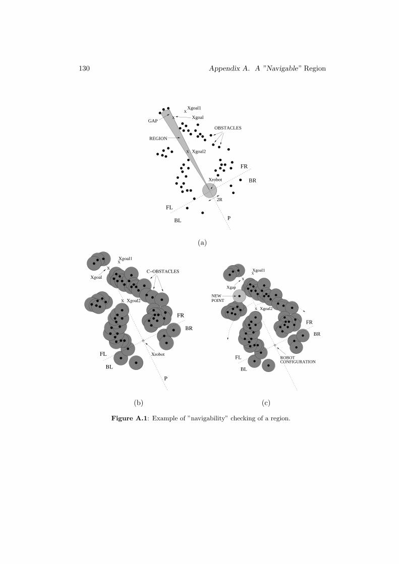
130 Appendix A. A ”Navigable” Region
FR
FL
BL
BR
XXgoal1
X Xgoal2
2R
OBSTACLES
X Xgoal
Xrobot
P
REGION
GAP
(a)
FR
FL
BL
BR
X
X
Xgoal2
Xgoal1
X
C−OBSTACLES
Xgoal
Xrobot
P
NEWPOINT
FR
FL
BL
BR
X
ROBOTCONFIGURATION
X
Xgoal2
Xgoal1
Xgap
X
(b) (c)
Figure A.1: Example of ”navigability” checking of a region.
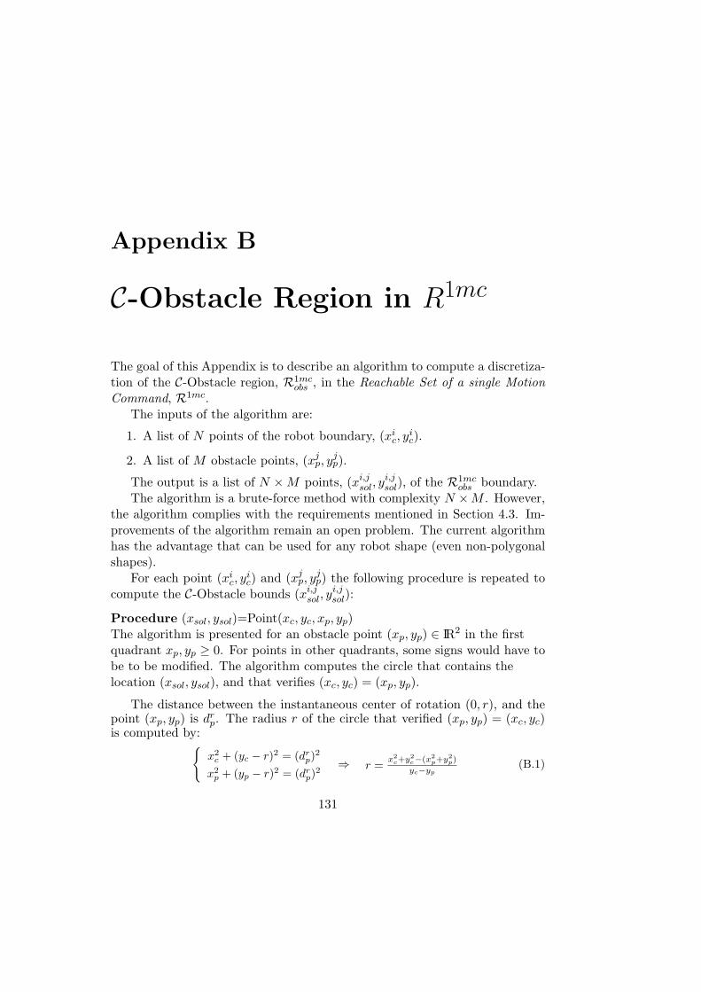
Appendix B
C-Obstacle Region in R1mc
The goal of this Appendix is to describe an algorithm to compute a discretiza-tion of the C-Obstacle region, R1mc
obs , in the Reachable Set of a single MotionCommand, R1mc.
The inputs of the algorithm are:
1. A list of N points of the robot boundary, (xic, y
ic).
2. A list of M obstacle points, (xjp, y
jp).
The output is a list of N ×M points, (xi,jsol, y
i,jsol), of the R1mc
obs boundary.The algorithm is a brute-force method with complexity N ×M . However,
the algorithm complies with the requirements mentioned in Section 4.3. Im-provements of the algorithm remain an open problem. The current algorithmhas the advantage that can be used for any robot shape (even non-polygonalshapes).
For each point (xic, y
ic) and (xj
p, yjp) the following procedure is repeated to
compute the C-Obstacle bounds (xi,jsol, y
i,jsol):
Procedure (xsol, ysol)=Point(xc, yc, xp, yp)The algorithm is presented for an obstacle point (xp, yp) ∈ IR2 in the firstquadrant xp, yp ≥ 0. For points in other quadrants, some signs would have tobe to be modified. The algorithm computes the circle that contains thelocation (xsol, ysol), and that verifies (xc, yc) = (xp, yp).
The distance between the instantaneous center of rotation (0, r), and thepoint (xp, yp) is dr
p. The radius r of the circle that verified (xp, yp) = (xc, yc)is computed by:
{x2
c + (yc − r)2 = (drp)
2
x2p + (yp − r)2 = (dr
p)2
⇒ r = x2c+y2
c−(x2p+y2
p)
yc−yp(B.1)
131
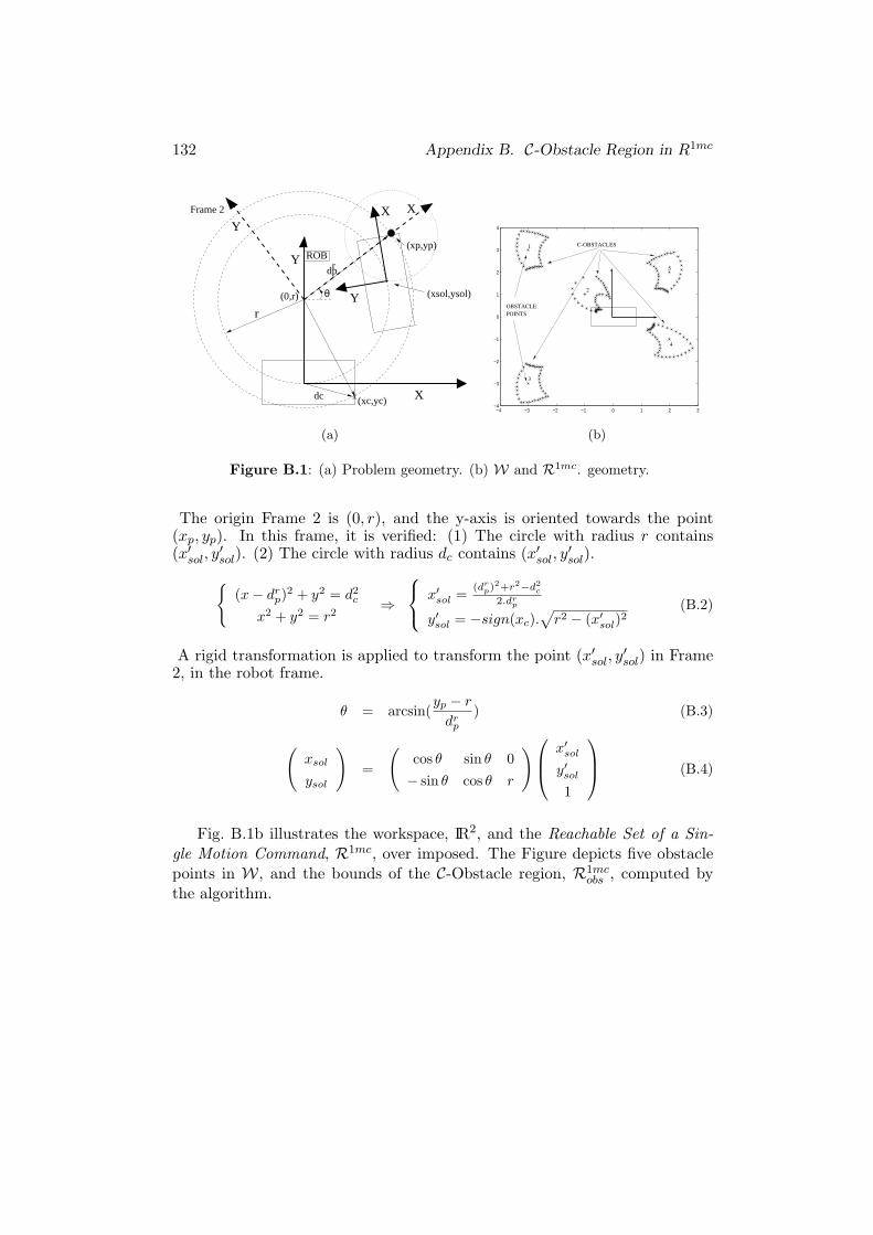
132 Appendix B. C-Obstacle Region in R1mc
x (xc,yc)dc
(xsol,ysol)
X
Y
Y
X
r
Y
X
dpr
(xp,yp)
θ
Frame 2
(0,r)
ROB
−4 −3 −2 −1 0 1 2 3−4
−3
−2
−1
0
1
2
3
4
1
2
3
4
5
C-OBSTACLES
OBSTACLE
POINTS
(a) (b)
Figure B.1: (a) Problem geometry. (b) W and R1mc. geometry.
The origin Frame 2 is (0, r), and the y-axis is oriented towards the point(xp, yp). In this frame, it is verified: (1) The circle with radius r contains(x′sol, y
′sol). (2) The circle with radius dc contains (x′sol, y
′sol).
{(x− dr
p)2 + y2 = d2
c
x2 + y2 = r2⇒
x′sol = (drp)2+r2−d2
c
2.drp
y′sol = −sign(xc).√
r2 − (x′sol)2(B.2)
A rigid transformation is applied to transform the point (x′sol, y′sol) in Frame
2, in the robot frame.
θ = arcsin(yp − r
drp
) (B.3)
(xsol
ysol
)=
(cos θ sin θ 0− sin θ cos θ r
)
x′sol
y′sol
1
(B.4)
Fig. B.1b illustrates the workspace, IR2, and the Reachable Set of a Sin-gle Motion Command, R1mc, over imposed. The Figure depicts five obstaclepoints in W, and the bounds of the C-Obstacle region, R1mc
obs , computed bythe algorithm.
Appendix C
The Selection of the Atan()Function
The goal of this Appendix is to justify the selection of the α = atan( Rrp
). Thisfunction converts R =]−∞,∞[ into an angular descriptor α = [−π
2 , π2 ].
rp = dm2 , with dm the diameter of the region to transform, see Fig. 4.3. The
function α = atan( Rrp
) converts into an angular index, α, the relation betweenthe circle with radius R and the circle with radius rp. In the following analysisthe case R > 0 is considered.
In sensor-based motion planning, a high resolution for radius close to rp
is required, and low resolution in the other case. (e.g rp = 2m is a typicalvalue. A turning radius R = rp ± 1m makes a big difference in the executedmotion. On the other hand, with rp = 100m, a turning radius R = 100m±1mmakes no difference, both radius produce roughly the straight motion.) Thisrequirement is fully verified by the selected function:
1. The region to transform (circumference with radius dm) is divided by rp
in four regions with the same area, see Fig. 4.3. The circles within R ∈[0, rp] and R ∈ [rp,∞[, that correspond to equal-area parts within theregion to transform, are mapped into equal-length intervals α ∈ [0, π/4]and α ∈ [π/4, π/2].
2. The resolution of the transformation is maximal for low values of R.Radius closed to rp are represented in more detail, as opposed to areas faraway from the vehicle. Fig. C.1a depicts the transformation. Fig. C.1bshows the same information, with the horizontal axis in logarithmic scale.In radius 0.1 < R
rp< 10 the angle varies in an approximate linear manner
in this scale.
133
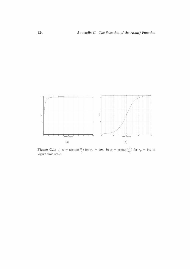
134 Appendix C. The Selection of the Atan() Function
0 10 20 30 40 50 60 70 80 90 1000
0.5
1
1.5
RADIUS (rp=1m)
alph
a
10−2
10−1
100
101
102
0
0.5
1
1.5
RADIUS (rp=1m)
alph
a
(a) (b)
Figure C.1: a) α = arctan( Rrp
) for rp = 1m. b) α = arctan( Rrp
) for rp = 1m inlogarithmic scale.
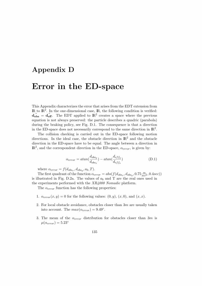
Appendix D
Error in the ED-space
This Appendix characterizes the error that arises from the EDT extension fromIR to IR2. In the one-dimensional case, IR, the following condition is verified:~dobs = ~deff . The EDT applied to IR2 creates a space where the previous
equation is not always preserved: the particle describes a quadric (parabola)during the braking policy, see Fig. D.1. The consequence is that a directionin the ED-space does not necessarily correspond to the same direction in IR2.
The collision checking is carried out in the ED-space following motiondirections. In the ideal case, the obstacle direction in IR2 and the obstacledirection in the ED-space have to be equal. The angle between a direction inIR2, and the correspondent direction in the ED-space, αerror, is given by:
αerror = atan(dobsy
dobsx
)− atan(deffy
deffx
) (D.1)
where αerror = f(dobsx , dobsy , ab, T ).The first quadrant of the function αerror = abs(f(dobsx , dobsy , 0.75 m
sec2, 0.4sec))
is illustrated in Fig. D.2a. The values of ab and T are the real ones used inthe experiments performed with the XR4000 Nomadic platform.
The αerror function has the following properties:
1. αerror(x, y) = 0 for the following values: (0, y), (x, 0), and (x, x).
2. For local obstacle avoidance, obstacles closer than 3m are usually takeninto account. The max(αerror) = 9.49◦.
3. The mean of the αerror distribution for obstacles closer than 3m isµ(αerror) = 5.23◦
135
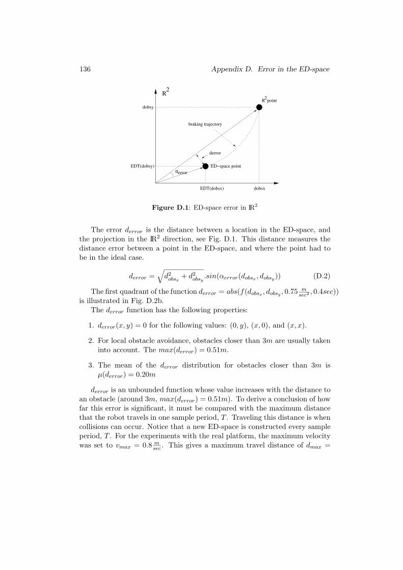
136 Appendix D. Error in the ED-space
R2
point
ED−space point
derror
R2
braking trajectory
dobsx
dobsy
errorα
EDT(dobsx)
EDT(dobsy)
Figure D.1: ED-space error in IR2
The error derror is the distance between a location in the ED-space, andthe projection in the IR2 direction, see Fig. D.1. This distance measures thedistance error between a point in the ED-space, and where the point had tobe in the ideal case.
derror =√
d2obsx
+ d2obsy
.sin(αerror(dobsx , dobsy)) (D.2)
The first quadrant of the function derror = abs(f(dobsx , dobsy , 0.75 msec2
, 0.4sec))is illustrated in Fig. D.2b.
The derror function has the following properties:
1. derror(x, y) = 0 for the following values: (0, y), (x, 0), and (x, x).
2. For local obstacle avoidance, obstacles closer than 3m are usually takeninto account. The max(derror) = 0.51m.
3. The mean of the derror distribution for obstacles closer than 3m isµ(derror) = 0.20m
derror is an unbounded function whose value increases with the distance toan obstacle (around 3m, max(derror) = 0.51m). To derive a conclusion of howfar this error is significant, it must be compared with the maximum distancethat the robot travels in one sample period, T . Traveling this distance is whencollisions can occur. Notice that a new ED-space is constructed every sampleperiod, T . For the experiments with the real platform, the maximum velocitywas set to vmax = 0.8 m
sec . This gives a maximum travel distance of dmax =
137
(a) (b)
Figure D.2: a) α = f(0 . . . 3, 0 . . . 3, 0.75 msc2 , 0.4sec). b) derror =
f(0 . . . 3, 0 . . . 3, 0.75 msc2 , 0.4sec)
vmax.T = 0.32m. For this distance, the maximum error is max(derror) =0.08m. Thus, the max(derror) in the reactive navigation context is low, andit can be neglected for collision checking. This error is comparable with othererrors such as uncertainties in the sensor measurements, the real controllers,controller time delays, and communications time delays among others.
This statement is used to extend the EDT to the two-dimensional casewith generality.

138 Appendix D. Error in the ED-space
Appendix E
The Robots
E.0.4 Nomadic XR4000
The Nomadic XR400 is a circular and holonomic robot. The robot diameteris 0.7m. The robot moves at omnidirectional translational velocities up to1.2 m
sec , and accelerations up to 1.5 msec2
. It is equipped with a SICK 2-D laserrangefinder with a field of view of 180◦, a range of 32 meters, an accuracy ofup to 1cm. Each laser scan has 361 points. See Fig. E.1a.
E.0.5 Labmate
The Labmate platform is an square and differential-driven robot. The robotside is 0.8m. The maximum speed is 1 m
sec . It is equipped with a TRC 3D laserrangefinder that scans the environment with a maximum range of 6.5m, andan accuracy up to 2.5cm. See Fig. E.1b.
E.0.6 Hilare2 and Hilare2Bis
The Hilare2 and Hilare2Bis platforms are rectangular and differential-driven.The robots are 1.3m × 0.8m. The maximum speed is 1.5 m
sec . Both robotsare equipped with a SICK laser rangefinder, see Subsection E.0.4. The maindifference between both robots is that Hilare2Bis is equipped with a GT6Aarm with 6 degrees of freedom. The arm weighs about 60kg and it is locatedin the front part of the robot. This produces a high inertia when the robotturns. See Fig. E.1c and Fig. E.1d.
139
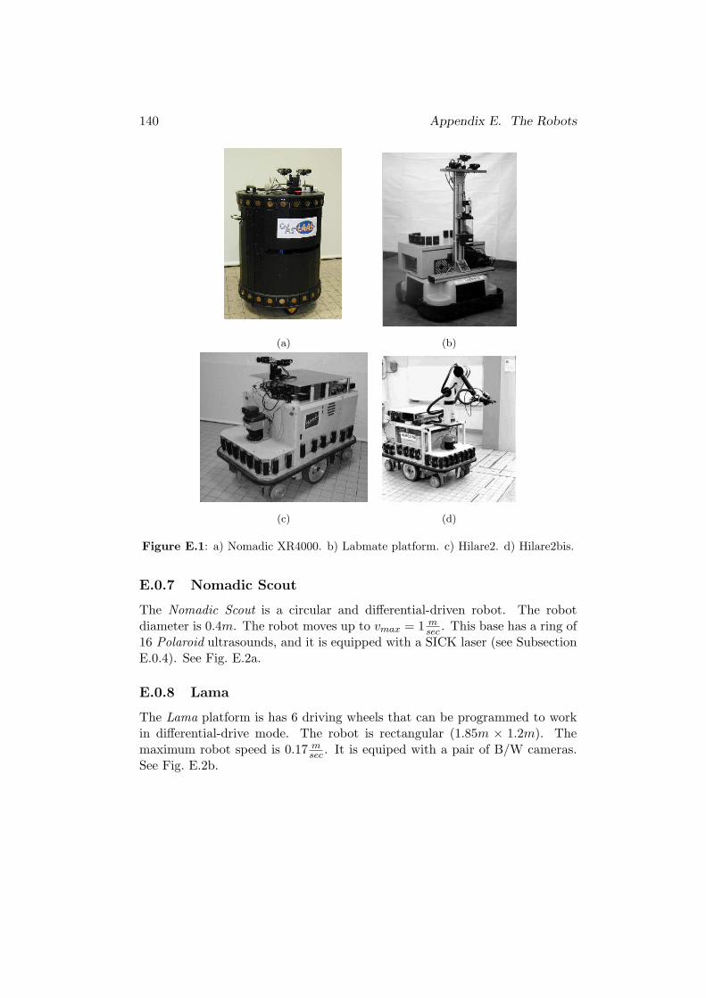
140 Appendix E. The Robots
(a) (b)
(c) (d)
Figure E.1: a) Nomadic XR4000. b) Labmate platform. c) Hilare2. d) Hilare2bis.
E.0.7 Nomadic Scout
The Nomadic Scout is a circular and differential-driven robot. The robotdiameter is 0.4m. The robot moves up to vmax = 1 m
sec . This base has a ring of16 Polaroid ultrasounds, and it is equipped with a SICK laser (see SubsectionE.0.4). See Fig. E.2a.
E.0.8 Lama
The Lama platform is has 6 driving wheels that can be programmed to workin differential-drive mode. The robot is rectangular (1.85m × 1.2m). Themaximum robot speed is 0.17 m
sec . It is equiped with a pair of B/W cameras.See Fig. E.2b.
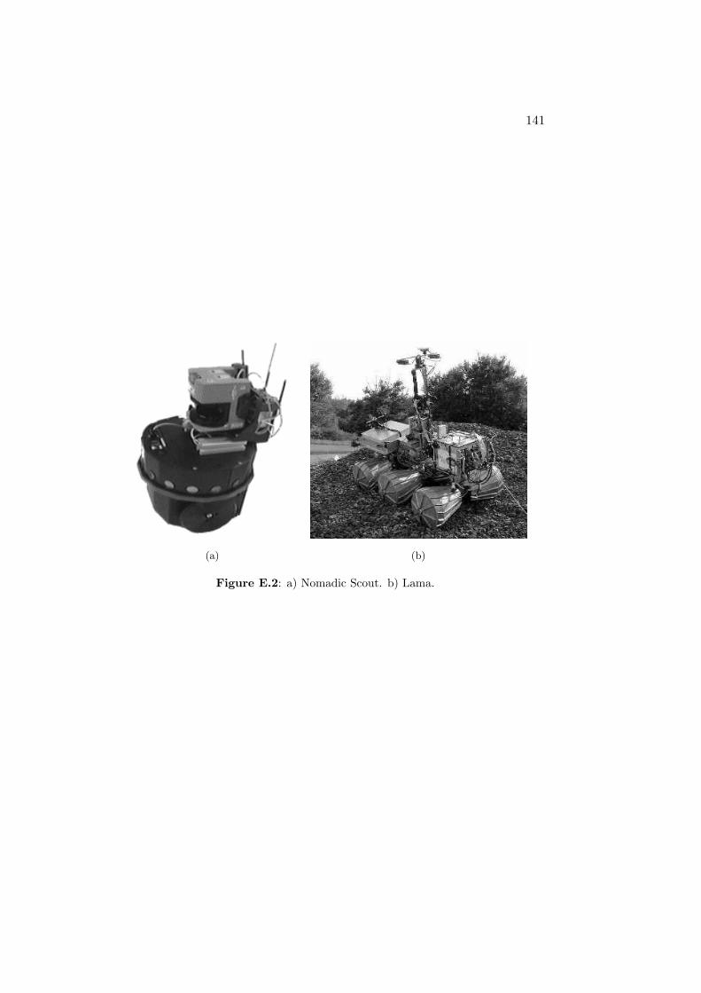
141
(a) (b)
Figure E.2: a) Nomadic Scout. b) Lama.