Robot Modeling - Optimization-based Robot Control

Robot Modeling

Optimization-based Robot Control

Andrea Del Prete

University of Trento

Schedule

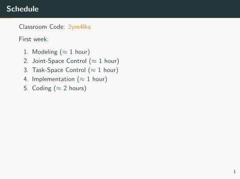
Classroom Code: 2ym4lka

First week:

1. Modeling (≈ 1 hour)

2. Joint-Space Control (≈ 1 hour)

3. Task-Space Control (≈ 1 hour)

4. Implementation (≈ 1 hour)

5. Coding (≈ 2 hours)

Second week:

1. Limits of Reactive Control (≈ 0.5 hour)

2. Linear Inverted Pendulum Model ≈ 0.5 hour)

3. Center of Mass Trajectory Generation (≈ 1 hour)


5. Coding: CoM trajectory optimization (≈ 1 hour)

6. Coding: walking with TSID (≈ 2 hours)

1

Schedule

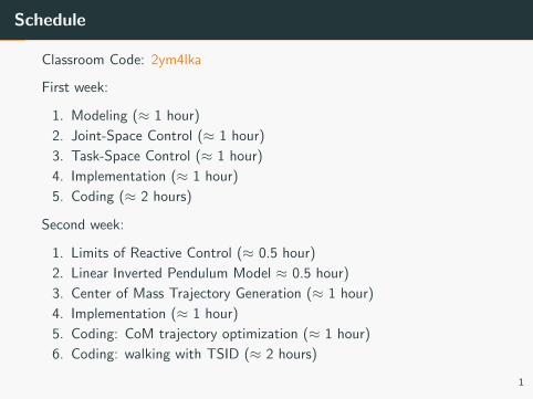
Classroom Code: 2ym4lka

First week:

1. Modeling (≈ 1 hour)

2. Joint-Space Control (≈ 1 hour)

3. Task-Space Control (≈ 1 hour)


5. Coding (≈ 2 hours)

Second week:

1. Limits of Reactive Control (≈ 0.5 hour)

2. Linear Inverted Pendulum Model ≈ 0.5 hour)

3. Center of Mass Trajectory Generation (≈ 1 hour)


5. Coding: CoM trajectory optimization (≈ 1 hour)

6. Coding: walking with TSID (≈ 2 hours)

1

Options for coding

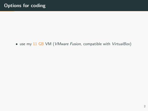
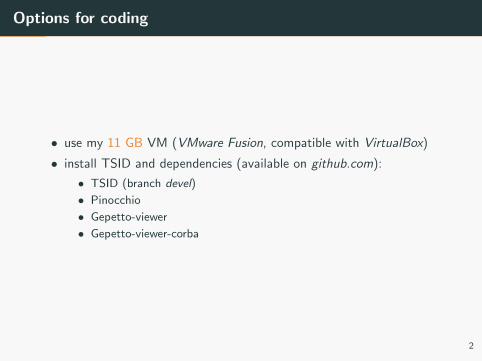
• use my 11 GB VM (VMware Fusion, compatible with VirtualBox)

• install TSID and dependencies (available on github.com):

• TSID (branch devel)

• Pinocchio

• Gepetto-viewer

• Gepetto-viewer-corba

2

Options for coding

• use my 11 GB VM (VMware Fusion, compatible with VirtualBox)

• install TSID and dependencies (available on github.com):

• TSID (branch devel)

• Pinocchio

• Gepetto-viewer

• Gepetto-viewer-corba

2

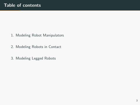
Table of contents

1. Modeling Robot Manipulators

2. Modeling Robots in Contact

3. Modeling Legged Robots

3

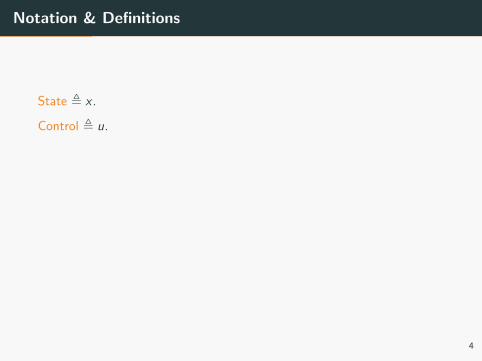
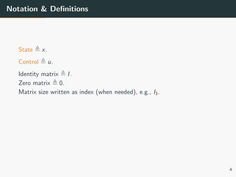
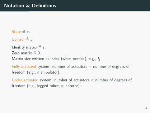
Notation & Definitions

State , x .

Control , u.

Identity matrix , I .

Zero matrix , 0.

Matrix size written as index (when needed), e.g., I3.

Fully actuated system: number of actuators = number of degrees of

freedom (e.g., manipulator).

Under actuated system: number of actuators < number of degrees of

freedom (e.g., legged robot, quadrotor).

4


State , x .

Control , u.


Zero matrix , 0.






4


State , x .

Control , u.


Zero matrix , 0.






4

Modeling Robot Manipulators

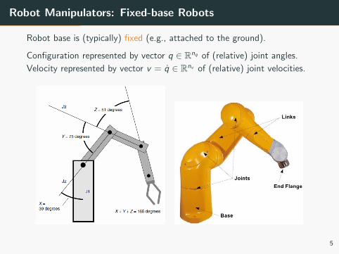
Robot Manipulators: Fixed-base Robots

Robot base is (typically) fixed (e.g., attached to the ground).

Configuration represented by vector q ∈ Rnq of (relative) joint angles.

Velocity represented by vector v = q ∈ Rnv of (relative) joint velocities.

5

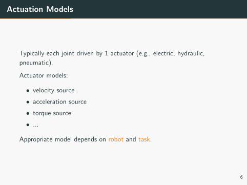
Actuation Models

Typically each joint driven by 1 actuator (e.g., electric, hydraulic,

pneumatic).

Actuator models:

• velocity source

• acceleration source

• torque source

• ...

Appropriate model depends on robot and task.

6

Actuation Models


pneumatic).

Actuator models:

• velocity source


• torque source

• ...


6

Actuation Models


pneumatic).

Actuator models:

• velocity source


• torque source

• ...


6

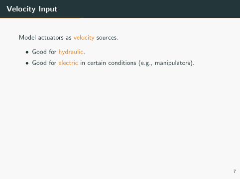
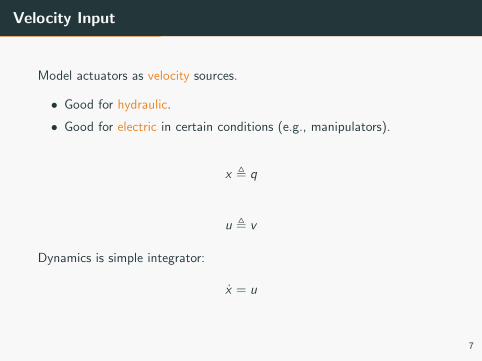
Velocity Input

Model actuators as velocity sources.

• Good for hydraulic.

• Good for electric in certain conditions (e.g., manipulators).

x , q

u , v

Dynamics is simple integrator:

x = u

7

Velocity Input

Model actuators as velocity sources.

• Good for hydraulic.

• Good for electric in certain conditions (e.g., manipulators).

x , q

u , v

Dynamics is simple integrator:

x = u

7

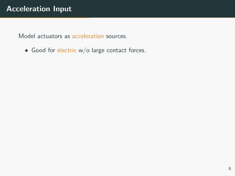
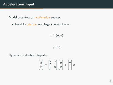
Acceleration Input

Model actuators as acceleration sources.

• Good for electric w/o large contact forces.

x , (q, v)

u , v

Dynamics is double integrator:[q

v

]=

[0 I

0 0

][q

v

]+

[0

I

]u

8

Acceleration Input

Model actuators as acceleration sources.

• Good for electric w/o large contact forces.

x , (q, v)

u , v

Dynamics is double integrator:[q

v

]=

[0 I

0 0

][q

v

]+

[0

I

]u

8

Torque Input

Model actuators as torque sources.

Good for electric w/o high-friction gear box—rarely the case

(unfortunately).

x , (q, v) u , τ

Dynamics of fully-actuated mechanical system (e.g., manipulator):

M(q)v + h(q, v) = τ,

where

• M(q) ∈ Rnv×nv , (positive-definite) mass matrix,

• h(q, v) ∈ Rnv , bias forces,

• τ ∈ Rnv , joint torques.

9

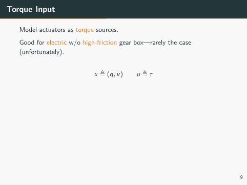
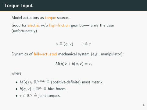
Torque Input

Model actuators as torque sources.

Good for electric w/o high-friction gear box—rarely the case

(unfortunately).

x , (q, v) u , τ

Dynamics of fully-actuated mechanical system (e.g., manipulator):

M(q)v + h(q, v) = τ,

where

• M(q) ∈ Rnv×nv , (positive-definite) mass matrix,

• h(q, v) ∈ Rnv , bias forces,

• τ ∈ Rnv , joint torques.

9

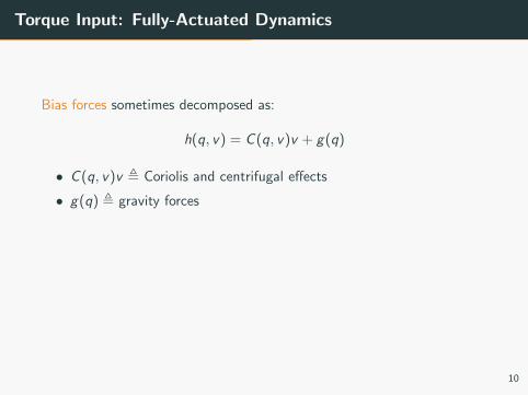
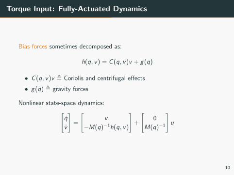
Torque Input: Fully-Actuated Dynamics

Bias forces sometimes decomposed as:

h(q, v) = C (q, v)v + g(q)

• C (q, v)v , Coriolis and centrifugal effects

• g(q) , gravity forces

Nonlinear state-space dynamics:[q

v

]=

[v

−M(q)−1h(q, v)

]+

[0

M(q)−1

]u

10

Torque Input: Fully-Actuated Dynamics

Bias forces sometimes decomposed as:

h(q, v) = C (q, v)v + g(q)

• C (q, v)v , Coriolis and centrifugal effects

• g(q) , gravity forces

Nonlinear state-space dynamics:[q

v

]=

[v

−M(q)−1h(q, v)

]+

[0

M(q)−1

]u

10

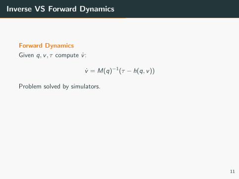
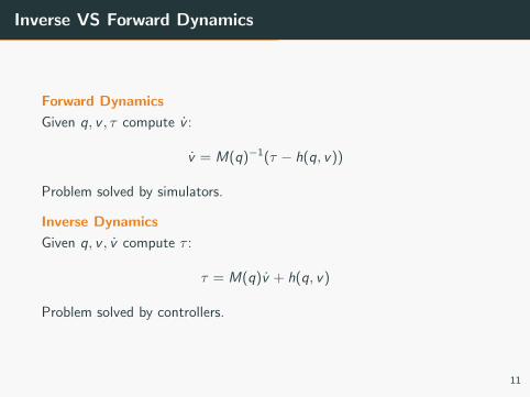
Inverse VS Forward Dynamics

Forward Dynamics

Given q, v , τ compute v :

v = M(q)−1(τ − h(q, v))

Problem solved by simulators.

Inverse Dynamics

Given q, v , v compute τ :

τ = M(q)v + h(q, v)

Problem solved by controllers.

11

Inverse VS Forward Dynamics

Forward Dynamics

Given q, v , τ compute v :

v = M(q)−1(τ − h(q, v))

Problem solved by simulators.

Inverse Dynamics

Given q, v , v compute τ :

τ = M(q)v + h(q, v)

Problem solved by controllers.

11

Modeling Robots in Contact

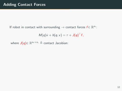
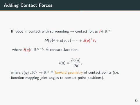
Adding Contact Forces

If robot in contact with surrounding → contact forces f ∈ Rnf :

M(q)v + h(q, v) = τ + J(q)>f ,

where J(q)∈ Rnf×nv , contact Jacobian:

J(q) =∂c(q)

∂q,

where c(q) : Rnq → Rnf , forward geometry of contact points (i.e.

function mapping joint angles to contact point positions).

12

Adding Contact Forces

If robot in contact with surrounding → contact forces f ∈ Rnf :

M(q)v + h(q, v) = τ + J(q)>f ,

where J(q)∈ Rnf×nv , contact Jacobian:

J(q) =∂c(q)

∂q,

where c(q) : Rnq → Rnf , forward geometry of contact points (i.e.

function mapping joint angles to contact point positions).

12

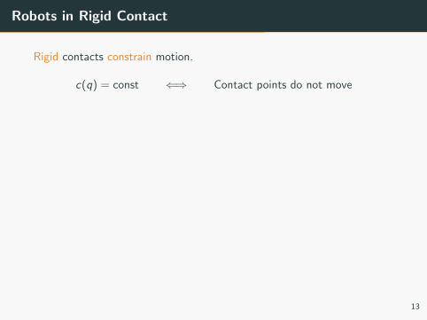
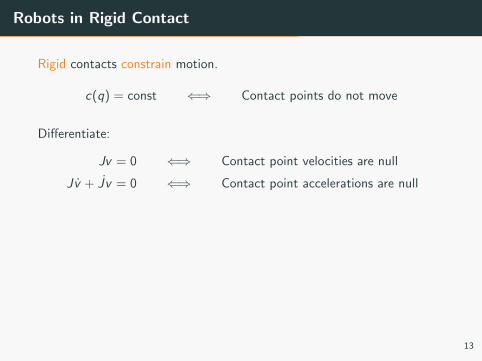
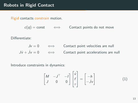
Robots in Rigid Contact

Rigid contacts constrain motion.

c(q) = const ⇐⇒ Contact points do not move

Differentiate:

Jv = 0 ⇐⇒ Contact point velocities are null

Jv + Jv = 0 ⇐⇒ Contact point accelerations are null

Introduce constraints in dynamics:

[M −J> −IJ 0 0

]vfτ

=

[−h−Jv

](1)

13




Differentiate:




[M −J> −IJ 0 0

]vfτ

=

[−h−Jv

](1)

13




Differentiate:




[M −J> −IJ 0 0

]vfτ

=

[−h−Jv

](1)

13




Differentiate:




[M −J> −IJ 0 0

]vfτ

=

[−h−Jv

](1)

13

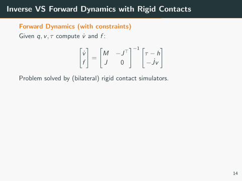
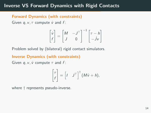
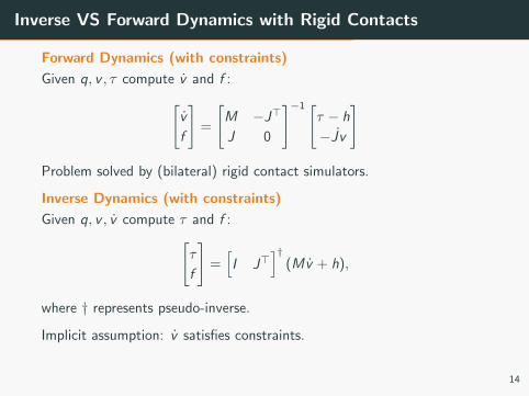
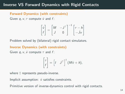
Inverse VS Forward Dynamics with Rigid Contacts

Forward Dynamics (with constraints)

Given q, v , τ compute v and f :[v

f

]=

[M −J>

J 0

]−1 [τ − h

−Jv

]

Problem solved by (bilateral) rigid contact simulators.

Inverse Dynamics (with constraints)

Given q, v , v compute τ and f :[τ

f

]=

[I J>

]†(Mv + h),

where † represents pseudo-inverse.

Implicit assumption: v satisfies constraints.

Primitive version of inverse-dynamics control with rigid contacts.

14




f

]=

[M −J>

J 0

]−1 [τ − h

−Jv

]




f

]=

[I J>

]†(Mv + h),




14




f

]=

[M −J>

J 0

]−1 [τ − h

−Jv

]




f

]=

[I J>

]†(Mv + h),




14




f

]=

[M −J>

J 0

]−1 [τ − h

−Jv

]




f

]=

[I J>

]†(Mv + h),



Primitive version of inverse-dynamics control with rigid contacts.14

Modeling Legged Robots

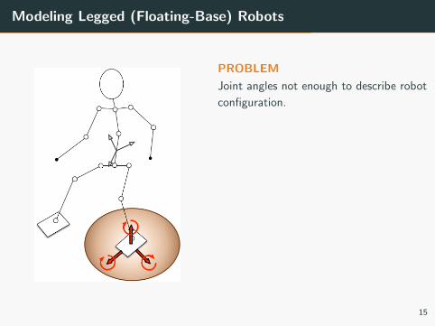
Modeling Legged (Floating-Base) Robots

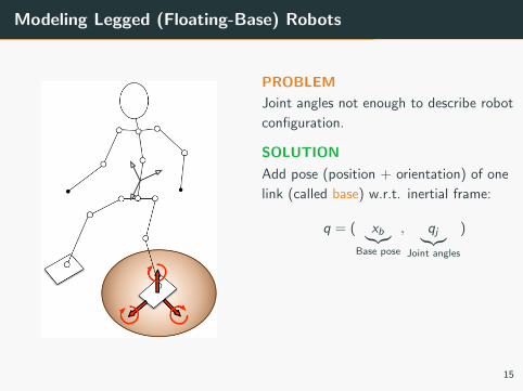
PROBLEM

Joint angles not enough to describe robot

configuration.

SOLUTION

Add pose (position + orientation) of one

link (called base) w.r.t. inertial frame:

q = ( xb︸︷︷︸Base pose

, qj︸︷︷︸Joint angles

)

Now q sufficient to describe robot

configuration in space.

15


PROBLEM


configuration.

SOLUTION





)



15


PROBLEM


configuration.

SOLUTION





)



15

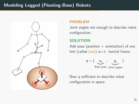
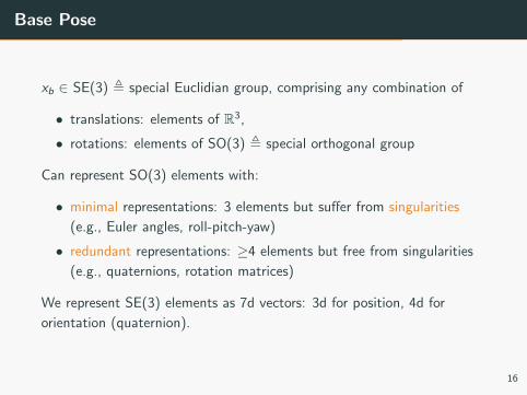
Base Pose

xb ∈ SE(3) , special Euclidian group, comprising any combination of

• translations: elements of R3,

• rotations: elements of SO(3) , special orthogonal group

Can represent SO(3) elements with:

• minimal representations: 3 elements but suffer from singularities

(e.g., Euler angles, roll-pitch-yaw)

• redundant representations: ≥4 elements but free from singularities

(e.g., quaternions, rotation matrices)

We represent SE(3) elements as 7d vectors: 3d for position, 4d for

orientation (quaternion).

16

Base Pose











16

Base Pose











16

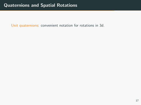
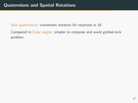
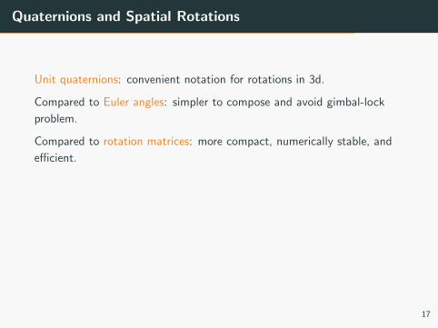
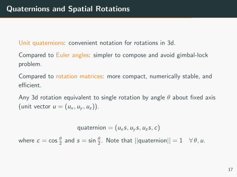
Quaternions and Spatial Rotations

Unit quaternions: convenient notation for rotations in 3d.

Compared to Euler angles: simpler to compose and avoid gimbal-lock

problem.

Compared to rotation matrices: more compact, numerically stable, and

efficient.

Any 3d rotation equivalent to single rotation by angle θ about fixed axis

(unit vector u = (ux , uy , uz)).

quaternion = (uxs, uy s, uzs, c)

where c = cos θ2 and s = sin θ2 . Note that ||quaternion|| = 1 ∀ θ, u.

17




problem.


efficient.





17




problem.


efficient.





17




problem.


efficient.





17

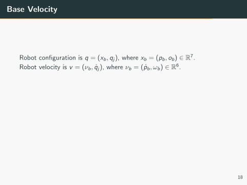
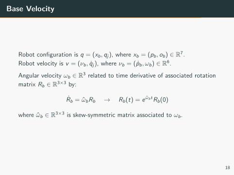
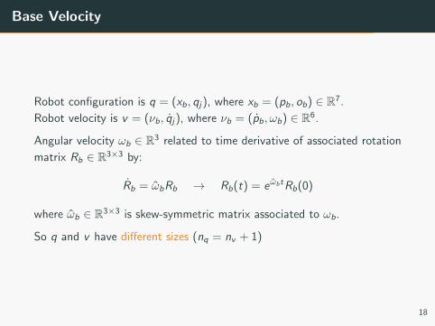
Base Velocity

Robot configuration is q = (xb, qj), where xb = (pb, ob) ∈ R7.

Robot velocity is v = (νb, qj), where νb = (pb, ωb) ∈ R6.

Angular velocity ωb ∈ R3 related to time derivative of associated rotation

matrix Rb ∈ R3×3 by:

Rb = ωbRb → Rb(t) = eωbtRb(0)

where ωb ∈ R3×3 is skew-symmetric matrix associated to ωb.

So q and v have different sizes (nq = nv + 1)

18

Base Velocity








18

Base Velocity








18

Base Velocity








18

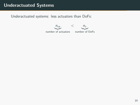
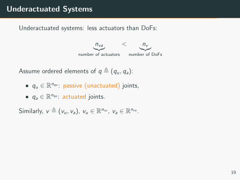
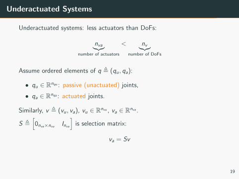
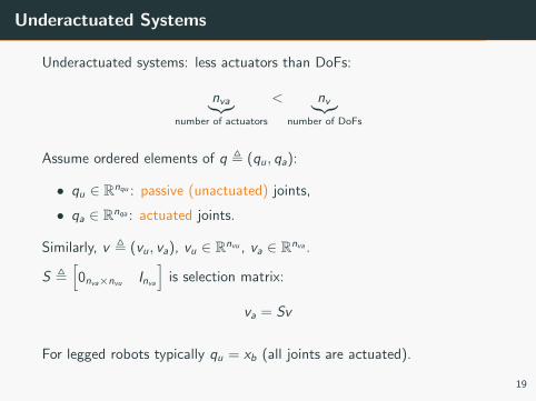
Underactuated Systems

Underactuated systems: less actuators than DoFs:

nva︸︷︷︸number of actuators

< nv︸︷︷︸number of DoFs

Assume ordered elements of q , (qu, qa):

• qu ∈ Rnqu : passive (unactuated) joints,

• qa ∈ Rnqa : actuated joints.

Similarly, v , (vu, va), vu ∈ Rnvu , va ∈ Rnva .

S ,[0nva×nvu Inva

]is selection matrix:

va = Sv

For legged robots typically qu = xb (all joints are actuated).

19









S ,[0nva×nvu Inva


va = Sv


19









S ,[0nva×nvu Inva


va = Sv


19









S ,[0nva×nvu Inva


va = Sv


19

Under-Actuated Dynamic

Dynamics of under-actuated mechanical system:

M(q)v + h(q, v) = S>τ + J(q)>f

Contrary to fully-actuated case: τ ∈ Rnva .

Often decomposed into unactuated and actuated parts:

Mu(q)v + hu(q, v) = Ju(q)>f

Ma(q)v + ha(q, v) = τ + Ja(q)>f(2)

where

M =

[Mu

Ma

]h =

[huha

]J =

[Ju Ja

](3)

20

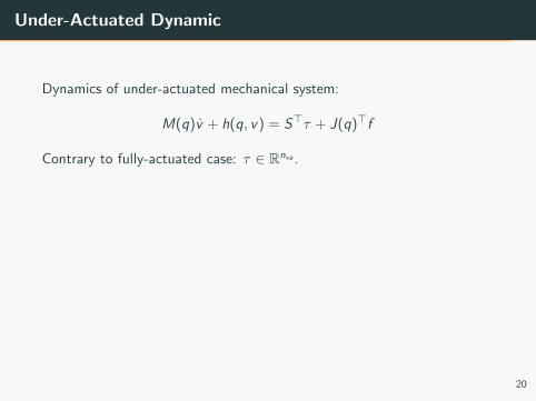
Under-Actuated Dynamic

Dynamics of under-actuated mechanical system:

M(q)v + h(q, v) = S>τ + J(q)>f

Contrary to fully-actuated case: τ ∈ Rnva .

Often decomposed into unactuated and actuated parts:

Mu(q)v + hu(q, v) = Ju(q)>f

Ma(q)v + ha(q, v) = τ + Ja(q)>f(2)

where

M =

[Mu

Ma

]h =

[huha

]J =

[Ju Ja

](3)

20

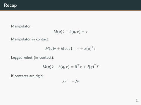
Recap

Manipulator:

M(q)v + h(q, v) = τ

Manipulator in contact:

M(q)v + h(q, v) = τ + J(q)>f

Legged robot (in contact):

M(q)v + h(q, v) = S>τ + J(q)>f

If contacts are rigid:

Jv = −Jv

21

Documents

Robot Modeling - Optimization-based Robot Control