Embed Size (px)
Citation preview

Robot ManipulatorsForward Kinematics of Serial Manipulators
Fig. 1: Stanford Arm
The focus of this module and the goal of forward kinematics (or direct kinematics) is obtaining
the position and orientation of the end-effector of a robot manipulator, with respect to a
reference frame, based on the orientations and configuration of the segments that comprise
the manipulator. This module introduces the Denavit-Hartenberg (DH) convention and
parameters that are used to describe these orientations and configurations, and provide a
standard approach to forward kinematics.
Links and Joints
Denavit-Hartenberg Convention
1. 1.
4. 4.
2. 2.
3. 3.
1. 1.
2. 2.
This is a convention used to attach a coordinate system to each link of a manipulator. The
coordinate systems are attached according to the following rules :
The origin of coordinate system is located at the point of intersection of the axis of
joint and the common normal between the axes of joints and .
The -axis is aligned with the axis of the joint. The positive direction of this
axis can be chosen arbitrarily.
The -axis is aligned with the common normal of the and joint axes and
points form the to the joint.
The -axis is determined using the right-hand rule.
The coordinate systems of the ground and end effector links do not follow these rules. The
coordinate system of the ground link can be chosen based on convenience as long as the
-axis is aligned with the axis of joint 1. The coordinate system of the end effector, also
called the hand coordinate system, can also be chosen based on convenience as long as its
-axis is normal to the last joint axis.
Denavit-Hartenberg Parameters
Any serial manipulator can be described kinematically by specifying four parameters for
each link.
Regardless of the physical construction of the actual link connecting two joints, their relative
location can be described using two parameters:
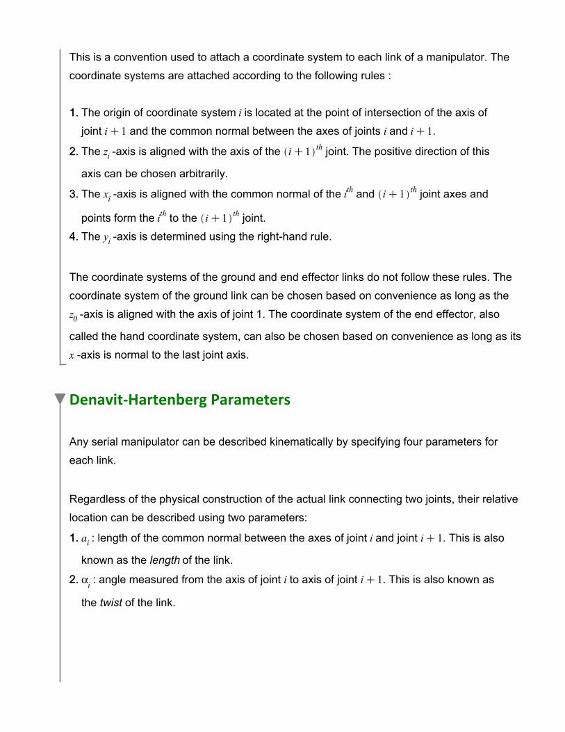
: length of the common normal between the axes of joint and joint . This is also
known as the length of the link.
: angle measured from the axis of joint to axis of joint . This is also known as
the twist of the link.
3. 3.
4. 4.
Fig. 3: Length and twist
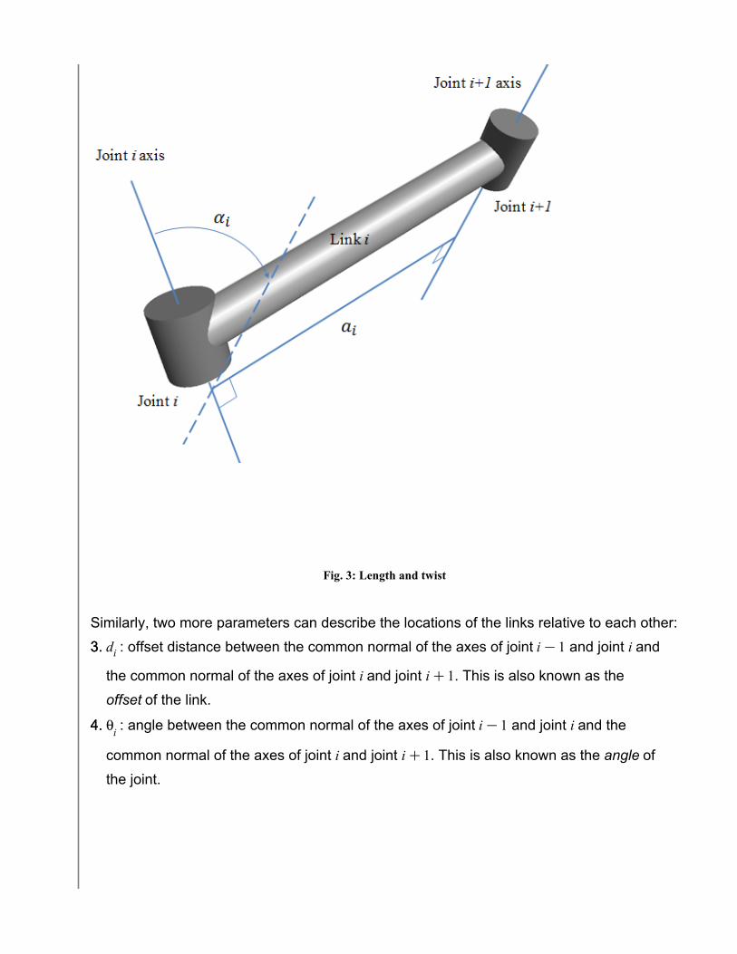
Similarly, two more parameters can describe the locations of the links relative to each other:
: offset distance between the common normal of the axes of joint and joint and
the common normal of the axes of joint and joint . This is also known as the
offset of the link.
: angle between the common normal of the axes of joint and joint and the
common normal of the axes of joint and joint . This is also known as the angle of
the joint.
2. 2.
1. 1.
Fig. 4: Offset and angle
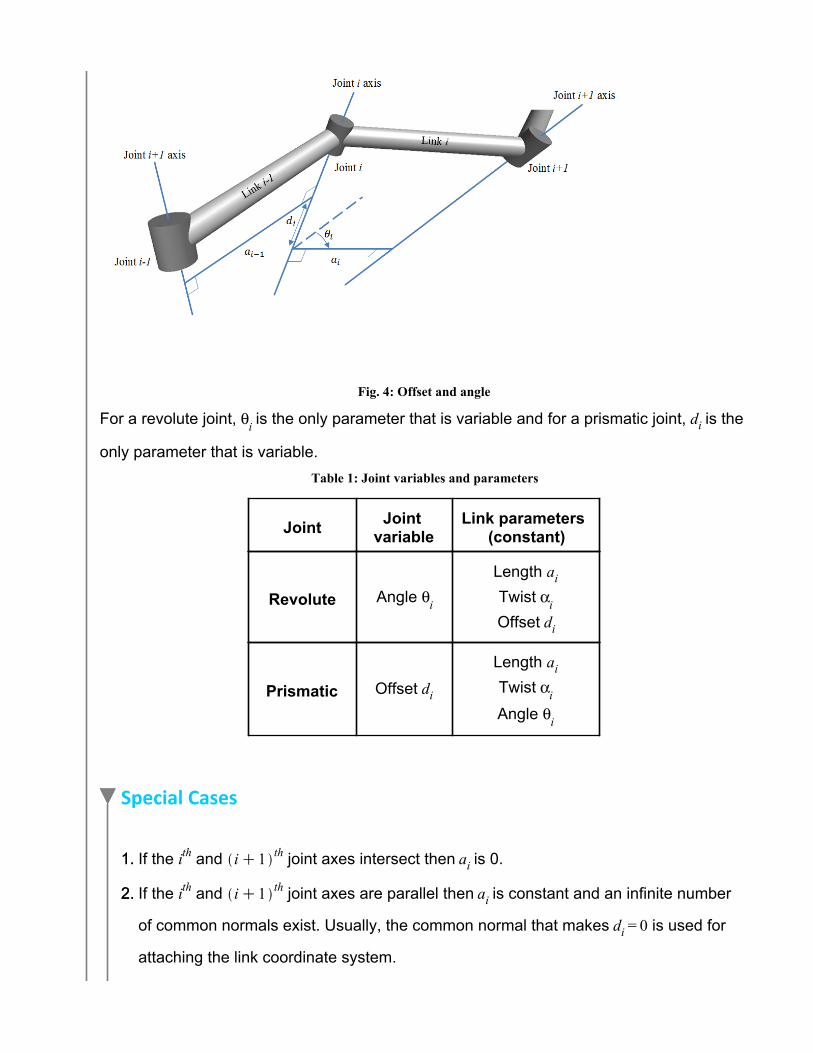
For a revolute joint, is the only parameter that is variable and for a prismatic joint, is the
only parameter that is variable.Table 1: Joint variables and parameters
Joint Joint variable
Link parameters (constant)
Revolute Angle Length Twist Offset
Prismatic Offset
Length Twist
Angle
Special Cases
If the and joint axes intersect then is 0.
If the and joint axes are parallel then is constant and an infinite number
of common normals exist. Usually, the common normal that makes is used for
attaching the link coordinate system.

1. 1.
2. 2.
3. 3.
3. 3.
If the and joint axes coincide then the origin of the coordinate system
is chosen arbitrarily. The choice of axes that makes most parameters 0 is
preferable.
Denavit-Hartenberg Homogeneous Transformation Matrices
Using the DH convention and parameters, transformation matrices relating two successive
coordinate systems can be established. The coordinate system can be obtained through
successive rotations and translations of the coordinate system:
The coordinate system is translated along the -axis by a distance . The
corresponding transformation matrix is
... Eq. (1)
The displaced coordinate system is rotated about the -axis by an angle . This
aligns the displaced -axis with the -axis. The corresponding transformation matrix
is
... Eq. (2)
The displaced coordinate system is translated along the -axis by a distance . The

3. 3.
4. 4.
3. 3.
corresponding transformation matrix is
... Eq. (3)
The displaced coordinate system is rotated about the -axis by an angle . This is the
final step that transforms the coordinate system to the coordinate system.
The corresponding transformation matrix is
... Eq. (4)
The resulting transformation matrix is
... Eq. (5)
which can be expanded to

3. 3.
3. 3.
... Eq. (6)
Multiplying this transformation matrix and the position vector of a point with respect to the
coordinate system will give the position vector of the point with respect to the
coordinate system.
Example 1: 3-DOF Planar Manipulator
A planar manipulator with 3 degrees of freedom is constructed with three revolute joints. A
reference coordinate system is attached to the base such that the manipulator moves in this
system's x-y plane. For this manipulator, all the twist angles and offset distances of the links
are equal to 0.
a) Find the DH transformation matrices , and in terms of the following joint
variables and link parameters:Table 2: 3-dof planar manipulator joint variables and link parameters
Joint
b) Find the position vector of the end-effector coordinate system with respect to the base
reference frame for the following values:Table 3: 3-dof planar manipulator joint variable and link parameter values

3. 3.
3. 3.
Joint
Analytical Solution
Part a) Transformation matrices in terms of joint variables and link parameters
Part b) Position vector of the origin of the end-effector coordinate system with respect to the base reference frame
Solution and visualization with MapleSim
Constructing the model
Create an "Axes" subsystem
Create a "revolute DH" subsystem
This subsections contains the steps to build a subsystem that can be used to build
the manipulator arm link by link using the DH parameters and variables.

3. 3.
3. 3.
4. 4.
1. 1.
5. 5.
3. 3.
2. 2.
Step 1: Insert components
Drag the following components into the main workspace:Table 5: Components and locations
Component Location
(3 required)
Multibody > Bodies and
Frames
(2 required)
Multibody > Visualization
Multibody > Joints and
Motions
Make 3 additional copies of the Axes subsystem.
A dialog box will appear while making copies of the subsystem. Select
Convert to a shared subsystem (Recommended). Selecting this option
causes any changes made to one subsystem to be automatically made to the
others.
Right click the fourth copy of the Axes subsystem and click Convert to Standalone Subsystem.
Double click this subsystem, change the radius of all its Cylindrical Geometry components to 0.02 m and all the radius at frame_a values of the

7. 7.
3. 3.
3. 3.
1. 1.
4. 4.
2. 2.
6. 6.
5. 5.
5. 5.
3. 3.
Tapered Cylindrical Geometry components to 0.04 m. This makes the axes
of this particular subsystem thicker. This modified Axes subsystem will be
used to visualize each link's coordinate system, and the other three axes
subsystems will be used to visualize the intermediate axes that show the
successive rotations and translations that transform one link's coordinate
system to the next link's coordinate system.
Step 2: Connect components
Arrange and connect the components as shown in the following diagram:
Fig. 8: Component diagram
Step 3: Create a subsystem
Select all the components and their connections.
Press Ctrl+G to create a subsystem.
Enter DH for the name of the subsystem and click OK.
Double-click the subsystem component created in the main workspace.
Connect the left port (frame_a) of RBF1 to a point on the dashed border on
the left, as shown in Fig. 9.
Connect the right port (frame_b) of RBF3 to a point on the dashed border on
the right, as shown in Fig. 9.
Connect flange_b of the Revolute component to a point on the top border, as

7. 7.
3. 3.
8. 8.
12. 12.
11. 11.
3. 3.
5. 5.
13. 13.
9. 9.
14. 14.
10. 10.
shown in Fig 9.
Fig. 9: DH subsystem
Click Add or Change Parameters in the Inspector pane of this subsystem.
Create parameters as shown in Fig. 10.
Fig. 10: DH parameters
Return to the diagram (click ), click RBF1 and enter [0,0,d_i] for the x,
y,z offset ( ).
Click RBF2 and enter [a_i,0,0] for the x,y,z offset ( ).
Click RBF3, enter [0,0,0] for the x,y,z offset ( ) and enter [alpha_i,0,0]
for the Rotations about the axes ( ).
Click CG1 , enter 0.008 m for the radius and change the color to purple.
Click CG2, enter 0.008 m for the radius and change the color to orange
9. 9.
1. 1.
7. 7.
3. 3.
3. 3.
11. 11.
10. 10.
5. 5.
7. 7.
14. 14.
2. 2.
4. 4.
5. 5.
6. 6.
8. 8.
3. 3.
(these CG components help visualize the link lengths and offsets).
Create a revolute joint visualization subsystem
Construct the manipulator
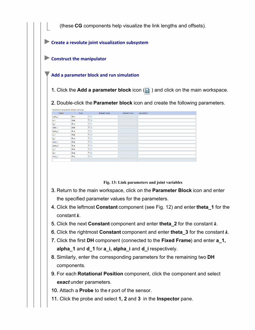
Add a parameter block and run simulation
Click the Add a parameter block icon ( ) and click on the main workspace.
Double-click the Parameter block icon and create the following parameters.
Fig. 13: Link parameters and joint variables
Return to the main workspace, click on the Parameter Block icon and enter
the specified parameter values for the parameters.
Click the leftmost Constant component (see Fig. 12) and enter theta_1 for the
constant .
Click the next Constant component and enter theta_2 for the constant .
Click the rightmost Constant component and enter theta_3 for the constant .
Click the first DH component (connected to the Fixed Frame) and enter a_1, alpha_1 and d_1 for a_i, alpha_i and d_i respectively.
Similarly, enter the corresponding parameters for the remaining two DH
components.
For each Rotational Position component, click the component and select
exact under parameters.
Attach a Probe to the r port of the sensor.
Click the probe and select 1, 2 and 3 in the Inspector pane.

12. 12.
7. 7.
3. 3.
3. 3.
14. 14.
15. 15.
5. 5.
16. 16.
14. 14.
13. 13.
Click the Absolute Translation Sensor and select Inertial for the Frame.
Click the Cylindrical Geometry components and change their color to
gray.
Reduce the Simulation duration to 1 sec (this is a static model).
Click Run Simulation ( ).
Use in the 3-D workspace toolbar to hide implicit geometry.
Fig. 14 shows the 3-D visualization of the MapleSim model. The intermediate coordinate
systems (thinner arrows) allow us to follow the successive rotations and translations of
the coordinate system that result in the coordinate system.
Fig. 14: 3-dof planar manipulator visualization
Fig. 15 shows the results of the simulation. These results match the answer obtained
analytically in part b) of the problem.

12. 12.
7. 7.
3. 3.
3. 3.
5. 5.
14. 14.
Fig. 15: 3-dof planar manipulator simulation results
The Constant components connected to the Rotational Position components can be
replaced with Ramp components to visualize the motion of the arm as the joint variables
change from 0 to the specified values. The following video shows this:

12. 12.
7. 7.
3. 3.
3. 3.
5. 5.
14. 14.
Video Player
Video 1: P3-dof planar manipulator motion visualization
The following diagram shows the modified component diagram with Ramp components.
12. 12.
7. 7.
3. 3.
3. 3.
5. 5.
14. 14.
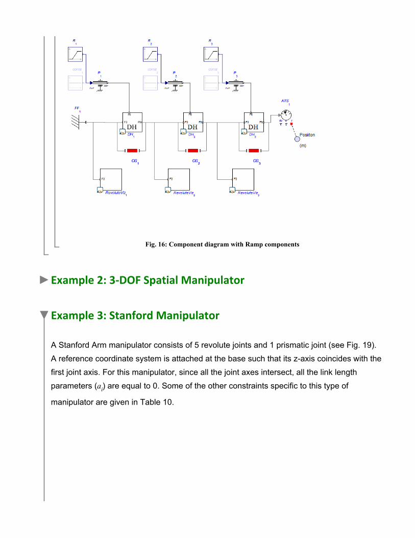
Fig. 16: Component diagram with Ramp components
Example 2: 3-DOF Spatial Manipulator
Example 3: Stanford Manipulator
A Stanford Arm manipulator consists of 5 revolute joints and 1 prismatic joint (see Fig. 19).
A reference coordinate system is attached at the base such that its z-axis coincides with the
first joint axis. For this manipulator, since all the joint axes intersect, all the link length
parameters ( ) are equal to 0. Some of the other constraints specific to this type of
manipulator are given in Table 10.

3. 3.
7. 7.
5. 5.
12. 12.
3. 3.
14. 14.
Fig. 19: Stanford Arm links and joints
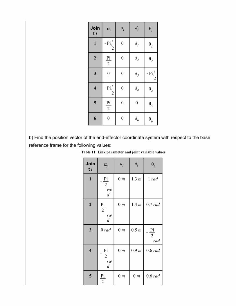
a) Find the DH transformation matrices , , , , and in terms of the following
joint variables and link parameters:Table 10: Link parameters and joint variables
3. 3.
7. 7.
5. 5.
12. 12.
3. 3.
14. 14.
Joint
b) Find the position vector of the end-effector coordinate system with respect to the base
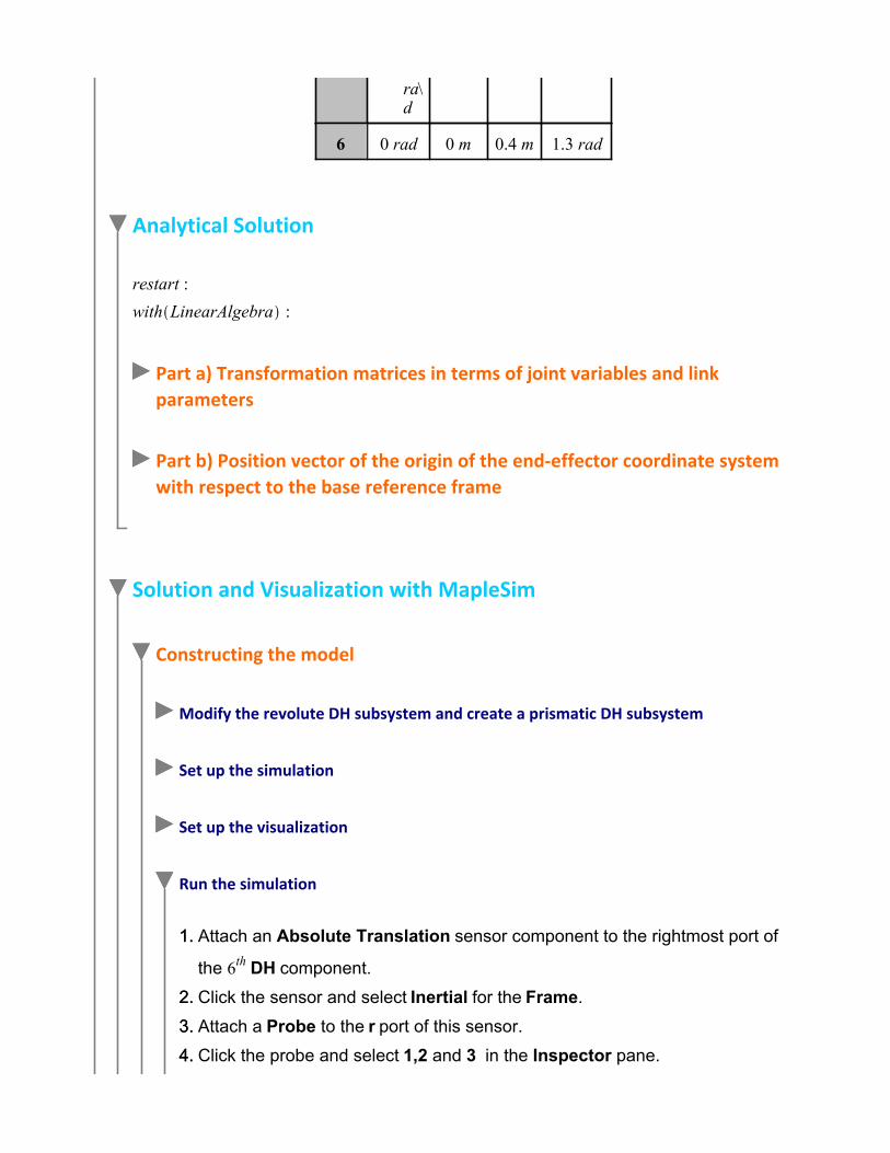
reference frame for the following values:Table 11: Link parameter and joint variable values
Joint
4. 4.
3. 3.
2. 2.
7. 7.
3. 3.
5. 5.
12. 12.
3. 3.
1. 1.
14. 14.
Analytical Solution
Part a) Transformation matrices in terms of joint variables and link parameters
Part b) Position vector of the origin of the end-effector coordinate system with respect to the base reference frame
Solution and Visualization with MapleSim
Constructing the model
Modify the revolute DH subsystem and create a prismatic DH subsystem
Set up the simulation
Set up the visualization
Run the simulation
Attach an Absolute Translation sensor component to the rightmost port of
the DH component.
Click the sensor and select Inertial for the Frame.
Attach a Probe to the r port of this sensor.
Click the probe and select 1,2 and 3 in the Inspector pane.
12. 12.
7. 7.
3. 3.
3. 3.
5. 5.
5. 5.
14. 14.
6. 6.
Reduce the Simulation duration to 1 sec (this is a static model).
Click Run Simulation ( ).
Similar to Examples 1 and 2, the Constant components connected to the Rotational Position components can be replaced with Ramp components to visualize the motion of
the arm as the joint variables change from 0 to the specified values. The following video
shows this motion:

12. 12.
7. 7.
3. 3.
3. 3.
5. 5.
5. 5.
14. 14.
Video Player
Video 3: Stanford arm motion visualization

12. 12.
7. 7.
3. 3.
3. 3.
5. 5.
5. 5.
14. 14.
Fig. 31 shows the simulation results of this simulation (using Ramp components). Each
joint variable changes linearly from 0 to its specified value over a period of 1 second. The
sequence of motions is in the same order as the joint numbering.
Fig. 31: Simulation results with motion
The position at the end of the simulation matches the position vector obtained in part b)
of the analytical solution.
References:1. L-W. Tsai. "Robot Analysis: The Mechanics of Serial and Parallel Manipulators". NY, 1999, John Wiley & Sons, Inc.2. W. W. Melek. "ME 547: Robot Manipulators: Kinematics, Dynamics, and Control". Waterloo, ON, 2010, University of Waterloo.