Robin Hood on the Grand CanalEconomic Shock and Rebellions in Qing China, 1650-1911 ∗

Yiming Cao †

Department of Economics

Boston University

Shuo Chen ‡

Department of Economics

Fudan University

October 14, 2017

Click Here for the Latest Version

Abstract

Social scientists have long pondered the effects of economic shocks on social conflict. How-

ever, the causal evidence discovered so far is limited to a small subset of economic shocks, and

the findings are still inconclusive. This paper uses the abandonment of China’s Grand Canal

— perhaps the largest infrastructure project in the pre-modern world — in 1826 as a natural

experiment to study the link between economic shocks and social conflicts. Using a dataset

covering 575 counties from 1650 to 1911, we find that negative economic shocks significantly

generated social instability: in the period after the canal’s abandonment, the annual frequency

of rebellions was 0.0094 higher in counties that bordered the canal than in those that did not.

The magnitude of the effect accounted for about 124% of the sample mean and was robust

across various specifications. We then compare the relative explanatory power of alternative

explanations, and conclude that the reform was most likely to trigger rebellions by reducing the

rebels’ opportunity costs, specifically by interrupting trade in urban areas. We briefly discuss

the possible implications in terms of the underlying social structure in urban regions, and tenta-

tively attempt to explore its persistent effects on gangs, secret societies and organized violence

in the 20th century.

Keywords: Economic Shocks; Conflict; Rebellions; the Grand Canal; China

JEL Classification Numbers: O13, O17, D74, H56, N45, N95, Q34.

∗Helpful and much appreciated suggestions, critiques and encouragement were provided by: Ying Bai, SamuelBazzi, Eli Berman, Travers Child, Zhao Chen, Zhiwu Chen, Esther Duflo, Thiemo Fetzer, Martin Fiszbein, OdedGalor, Yu Hao, James Kung, Xiaohuan Lan, Pinghan Liang, Ruobing Liang, Gedeon Lim, Chicheng Ma, RobertMargo, Tianguang Meng, Nathan Nunn, Nancy Qian, Zheng Song, Shangjin Wei, Austin Wright, Chenggang Xu,Noam Yuchtman; participants of 2016 NBER Chinese Studies Group meeting, the 4th International Symposium onQuantitative History, NEUDC 2016 at MIT, NBER Summer Institute 2017, seminar participants at Boston Univer-sity, Fudan University, Harvard University, Jinan University, Peking University, Shandong University, SouthwesternUniversity of Finance and Economics and Tsinghua University.

†Address: 270 Bay State Road,Boston, MA 02215, USA, e-mail: yiming@bu.edu.‡Address: 600 GuoQuan Road, Yangpu District, Shanghai, 200433, China, e-mail: cs@fudan.edu.cn.

In the eastern provinces of China, too, several great rivers form, by their different

branches, a multitude of canals, and, by communicating with one another, afford an

inland navigation much more extensive than that either of the Nile or the Ganges, or,

perhaps, than both of them put together.

—Adam Smith (1776)

1 Introduction

Social scientists have long pondered the effects of economic shocks on social conflict. They have

provided substantial evidence that these two factors are negatively correlated (Collier and Hoeffler,

1998, 2004; Fearon and Laitin, 2003; Humphreys, 2005; Buhaug and Rød, 2006; Ross, 2006; Angrist

and Kugler, 2008; Bellows and Miguel, 2009; Kung and Ma, 2014a). An emerging literature seeks

to isolate exogenous variations to identify their causality. However, most of the causal evidence is

limited to climate shocks on agricultural productivity (Miguel et al., 2004; Miguel, 2005; Mehlum

et al., 2006; Miguel, 2007; Burke et al., 2009; Miguel and Satyanath, 2011; Ciccone, 2008) and

price shocks to global commodities (Besley and Persson, 2008; Brckner and Ciccone, 2010; Dube

and Vargas, 2013), and the findings are still inconclusive (Bazzi and Blattman, 2014; Burke et al.,

2015; Sarsons, 2015). This paper attempts to contribute to the literature using a novel natural

experiment – the abandonment of China’s Grand Canal in 1826 – to examine the link between

economic shocks and social conflicts.

The Grand Canal is perhaps the largest and oldest infrastructure in the pre-modern world. It

spans 1, 776 km (1, 104 miles) in length, passing through six provinces in the north-eastern and

central-eastern plains of China. This area was populated by over 126 million inhabitants in the

early 19th century, accounting for about 15% of the world’s population. The first parts of the

canal date back to the 5th century BC, while the various sections were finally integrated into a

nationwide system during the Sui Dynasty (581–618 AD). The primary purpose of the canal was

to transport tribute grain — the most important grain tax — from southern China to Beijing, the

capital city of the empire. In early 19th century, approximately 3.5 million piculs of rice (roughly

560 million lbs) were delivered annually. The canal also benefited the adjacent regions by reducing

the transport costs for long-distance trade. Grain junks were allowed to carry set amounts of duty-

free commodities during their service, and private junks used the canal extensively for trade, travel

and pleasure. The Grand Canal thus developed into one of China’s most popular trade routes.

Starting in 1826, the Qing government gradually abandoned the Grand Canal as the exclusive

route for tribute grain transportation and stopped maintaining it. This change resulted in a drastic

decline in trade around the canal. The dismissal of official grain junks directly reduced the number

of commodities transported on the canal, and private trade suffered as the canal became clogged

with silt. By the early 20thcentury, much of the canal was no longer navigable, which resulted

in the general decline of the canal corridor economic belt. Historians have long argued that the

abandonment of the canal was responsible for the subsequent wave of social unrest in late Qing

2

Dynasty (Esherick, 1988), yet this hypothesis has never been systematically tested.

The abandonment of the canal provides an ideal opportunity to study the link between economic

shocks and social conflicts for three main reasons. First, the reform was unexpected, and was

primarily based on the political, rather than economic, considerations of the new emperor. This

provides plausibly exogenous shocks to the local economy. Second, there is rich information available

on social unrest in historical China over a long period of time. We constructed an original dataset

consisting of 575 counties over 262 years (from 1650 to 1911). It is based on the historical records

officially compiled by the Qing Court, which provided detailed information on the time, location

and activities for each rebellion throughout the Qing Dynasty. Lastly, by focusing on variations

within a single country, our sample is relatively homogeneous with respect to ethnicity, institution

and culture, which are important factors in the conflict literature (Hegre and Sambanis, 2006;

Laitin, 2007; Djankov and Reynal Querol, 2010; Kung and Ma, 2014b; Janus and Riera-Crichton,

2015; Jha, 2013).

We begin our analysis with a standard differences-in-differences (DID) strategy. Specifically,

we compare the relative change in the number of rebellions in counties along the canal relative

to non-canalside counties. Our findings across various specifications suggest a higher number of

rebellions associated with the canal’s abandonment: compared to non-canalside counties, those

bordering the canal experienced 0.0094 more rebellions after the reform (relative to before). The

effect corresponds to a 124% increase relative to the sample mean (0.0076), and is significant at

the 95% confidence interval.

We then refine the baseline model with binary treatment by allowing continuous measures of

intensity. To this end, we exploit two sources of cross-county variations: (i) the length of the

canal within a county and (ii) the distance from the county to the canal. Consistent with our

expectations, we find that the number of rebellions increases with the length of the canal within

the county, and decreases with distance from the county to the canal. Estimates from more flexible

specifications further verify that these effects are specific to counties within 150 km of the canal.

We interpret this as the range of the canal’s impact.

In order to take into account the canal’s gradual abandonment, we extend the two-period

model to continuous measures of reform progress. The most natural way to do so is to use the

number of years since the reform as a linear measure of completeness. The results suggest that the

impact increases as the reform unfolds. More flexible decade-by-decade estimates allow us to further

explore the nonlinear dynamics of rebellions over time. After the canal’s abandonment, the number

of rebellions kept increasing for over 30 years. Then the effect appears to fade, but it remained

positive and significant throughout our study period. In this specification, the coefficients estimated

for periods prior to the reform also serve as a verification of the common trends assumption that

validates our identification method.

We conducted several robustness checks to assess the quality of the previous identification. To

address concerns that our results suffer from omitted variable bias, we include a set of control

variables from the literature on the determinants of conflict: weather, geography, agricultural

3

technology and culture. Our results are robust to the inclusion of all these factors. To explore

whether there is reverse causality in the later periods of the sample, we restrict our analysis to

truncated sample periods, and the results confirm that our findings are not affected by excluding

potentially endogenous periods. Finally, to avoid the spurious correlations due to noise, we conduct

a falsification test that compares the estimated treatment effects with the distribution of placebo

treatment effects when county locations are randomly assigned. The results of the falsification test

confirm that it is unlikely that noise in the data is affecting our results.

What are the mechanisms underlying the the observed effects? We investigate two hypotheses

proposed in the conflict literature: (i) the decline in state capacity and (ii) the reduction in oppor-

tunity costs. After comparing the evidence regarding competing theories’ explanatory power, we

find that the opportunity cost hypothesis appears to be more consistent with what we observe in

the data. In particular, the increase in rebellions in counties bordering the canal seems to have

been due to the interruption of trade in urban sectors. We briefly discuss the possible implica-

tion in terms of the underlying social structure in urban regions, and relate this to the evolution

of gangsters, the emergence of communism in the early 20th century, and the presence of armed

conflicts during the Cultural Revolution.

Our study contributes to the emerging literature on the causal relationship between economic

shock and conflict (See Blattman and Miguel (2010) for an overview), which primarily focuses on

economic shocks associated with weather volatility (Miguel et al., 2004; Miguel, 2005; Mehlum

et al., 2006; Miguel, 2007; Burke et al., 2009; Miguel and Satyanath, 2011; Ciccone, 2008) and

commodity price (Besley and Persson, 2008; Brckner and Ciccone, 2010; Dube and Vargas, 2013).

Such shocks, while causally well-identified, represent a narrow subset of economic shocks that is

transitory, rural specific, and not policy relevant. This paper examines the effects of permanent

shocks initiated by government policy on the urban sector, which has distinct implications that are

rarely documented in previous studies. First, while transitory shocks only change current economic

conditions, permanent ones affect all subsequent periods as well as people’s expectations about the

future 1. Consistent with Iyigun et al. (2017), we find that conflicts induced by a permanent shock

tend to be very frequent and persistent. Second, unlike their rural counterparts, the labor force in

densely populated urban areas has more collective consciousness and organized politics. Such areas

are likely to become hotbeds of gangsters and organized crimes if there is a lack of socio-economic

opportunities. This pattern, which is confirmed in our data, is consistent with case studies on the

evolution of gangs and the mafia in the United States (Haller, 1971; Hagedorn and Macon, 1988;

Critchley, 2008). Finally, our findings suggest that openness to trade is a potential policy approach

to preventing violent conflict.

This paper is also related to the impact of transportation infrastructure. Economic histori-

ans have documented extensive evidence regarding the impact of transportation infrastructure,

particularly the building of highways and railroads (Fogel, 1979, 1994; Fernald, 1999; Haines and

1It is unclear whether a permanent shock would exhibit more or less detrimental effects than the transitory shocks,due to the interplay of “adaptation” and “intensification” effects. See Iyigun et al. (2017) for a detailed discussion ofthese two terms.

4

Margo, 2006; Baum-Snow, 2007; Atack et al., 2008; Michaels, 2008; Atack et al., 2010; Duranton

and Turner, 2012; Donaldson, forthcoming; Donaldson and Hornbeck, forthcoming; Perlman, 2016)

. While most of them focus on the economic consequences, we provide evidence of the non-economic

consequences of transportation infrastructure. Recent work exploring this topic includes Sokoloff

(1988), Burgess and Donaldson (2010), Agrawal et al. (2017), and Perlman and Schuster (forth-

coming). Our paper also departs from the existing literature by focusing on abandonment rather

than construction. Policy makers should take into account the detrimental effect of infrastructure

abandonment revealed in our analysis.

The canal’s abandonment appears to have produced persistent effects on secret societies and

organized violence in the 20th century, which speaks to the growing literature on the legacies of

historical events (See Nunn (2009) for a decent review). Several channels behind such persistence

have been well explored, from formal institution (Sokoloff and Engerman, 2000; Acemoglu and

Robinson, 2001; Dell, 2010), to culture (Tabellini, 2008; Fernndez and Fogli, 2009; Tabellini, 2010;

Nunn and Wantchekon, 2011; Voigtlander and Voth, 2012; Grosjean, 2014; Chen et al., 2017) and

genetics (Ashraf and Galor, 2013; Arbatli et al., 2015; Galor and Klemp, 2017). Our findings, while

preliminary, highlight the role of social structure as another possible channel. In this sense, it follows

the idea proposed by Moscona et al. (2017), which establishes segmentary lineage organization in

Sub-Saharan Africa as a predictor of modern civil wars.

This paper also offers an alternative explanation of the waves of China’s substantial social unrest.

A growing literature shows that conflicts throughout China’s history have been significantly related

to variations in climate (Bai and Kung, 2011; Chen, 2015), technology (Jia, 2014) and social norms

(Kung and Ma, 2014b). This paper suggests government policies have also been responsible. In

this sense, our research is closely related to Bai and Jia (2016), who attribute China’s political

instability in the early 20th century to the 1905 abolition of the civil service exam.

The remainder of the paper is organized as follows. The next section presents the background of

the Grand Canal and its abandonment. Section 3 presents the data, while Section 4 formalizes our

empirical strategy and demonstrates the baseline results. Section 5 describes the robustness checks.

Section 6 discusses the possible mechanisms and their implications, and Section 7 concludes.

2 Background

2.1 The Grand Canal

The 1, 776 km Grand Canal is the longest and oldest artificial waterway in the world. Located in

the north-eastern and central-eastern plains of China, it links Beijing in the north with Hangzhou

in the south (see Figure 1)2. Construction of the first parts of the canal date back to the 5th

century BC, while the various sections were finally integrated into a nationwide system during the

Sui Dynasty (581–618 AD). Its scale was unparalleled in its time (Elvin, 1973). More than 126

2The canal cuts across four provinces (Zhili (now Hebei), Shandong, Jiangsu, and Zhejiang) and runs very closeto Henan and Anhui

5

million people lived in the six canalside provinces in 1820, which accounted for about 15% of the

world’s population.

The canal was originally constructed to secure the food supply of China’s capital and most

populous city, Beijing, which had a population of over a million in 1820. Many of its residents

consisted of the court, official personnel, scholars, imperial soldiers and their families (Morse, 1913;

Chi, 1936), and did not produce their own rice. Rice production was clustered in the southern

part of China where there was abundant, fertile land and suitable weather (rain and sunshine) for

agriculture 3. Therefore a huge amount of rice was shipped to the capital, primarily via the Grand

Canal. In the early 19th century, approximately 3.5 million piculs of rice (roughly 560 million

pounds) were delivered to the capital annually (Huang, 1918). Maintaining the well-functioning

of the canal was one of the most crucial tasks for the Qing government (Hummel, 1991; Leonard,

1988; Cheung, 2009).

The canal also benefited the adjacent regions by facilitating regional trade and providing urban

employment. The government allowed the grain junks to carry an estimated 200 million pounds

of duty-free commodities annually in the early 19th century (Ni, 2005). The popular commodities

ranged from bamboo, woods, paper, china and silk to pears, jujube and walnuts. Private junks

also used the canal extensively for trade, travel and pleasure (Gandar, 1894; Hinton, 1952). A total

of over 10 million piculs (roughly 1.5 billion pounds) of commodities were transported along the

canal each year. The Grand Canal also created numerous jobs in urban areas. Workers were hired

either by the government in boat construction and canal maintenance, or by the private sector in

restaurants, hotels and commercial services.

The Grand Canal thus boosted the economy along its route and created large commercial cities.

For example, Linqing was a minor county before the construction of the canal. It developed into

a trade center by the early Qing Dynasty, and was promoted to a municipality in 1777. The

prosperity of the corridor was also reflected in its population density. In 1820, the population

density in prefectures along the canal was 45% higher than non-canalside prefectures.

2.2 Abandonment of the Grand Canal

The canal was gradually abandoned after 1826 as part of a reform initiated due to a combination

of natural and human factors. In 1825, the breach of the embankment dam at the intersection

between the Yellow River and the canal temporarily interrupted grain transportation via the canal.

Daoguang Emperor (1821 – 1850), the 7th emperor of the Qing Dynasty, unexpectedly decided

to abandon the Grand Canal and use the east-China Sea route instead. This decision was more

political than economic because this shift gave the new emperor the opportunity to appoint his

trusted followers and to establish his own authority. The canal was abandoned gradually rather

than rapidly due to safety considerations.

In 1826, the government experimented with shipping 1.63 million piculs (roughly 260 million

3Figure B1 shows the suitability index for wetland rice farming in China. Most areas around Beijing are notsuitable for growing rice. The most suitable lands are cluster in the south.

6

pounds) of tribute rice collected in Jiangsu by sea. It was first shipped from Shanghai to Tianjin

in 1,562 chartered ships, and then conveyed to Beijing (Hinton, 1952). The sea transportation area

expanded to Jiangsu and Zhejiang after 1852, which accounted for half the amount of rice in the

tribute grain system. The lack of use led to negligence in the canal’s maintenance, which worsened

its condition. The government officially announced the canal’s abandonment in 1901 when much

of it had become too clogged to navigate. Figure B3 plots the amount of tribute rice shipped via

the canal using a 5-year moving average. Although the amount fluctuated over time, there was a

consistent drop in the amount shipped via the canal right after the 1826 experiment. Therefore,

we use 1826 as the first post reform year in our baseline analysis 4.

The abandonment of the Grand Canal inevitably led to the decline of the economic belt that

had developed alongside it. As the only north-south waterway in east China, the reform forced

most commodities to be transported by land, which was 9-10-fold more costly in pre-modern China

(Watson, 1972; Shiue, 2002). Meanwhile, jobs that relied on the canal trade disappeared, the

economies of the regions near the canal declined, and unemployment increased. As shown in Figure

2, regions adjacent to the canal did not recover from this recession until the early 20th century.

The population of Linqing fell from over 200, 000 in the late 18th century to less than 50, 000 by

the early 20th century (Cao, 2001).

There is considerable anecdotal evidence that the canal’s abandonment led to great social disor-

der in the region. For example, a 19th century ballad popular in Shandong called “Broken the boat,

disordered the world” lamented the destructive consequences of the closure of the canal. Esherick

(1988) argues that the disruption of the canal was responsible for the Boxer Rebellions in the late

19th century. Another famous example is the Green Gang, the prominent criminal organization

in the early 20th century formed by workers who lost their jobs due to the closure of the canal

(Martin, 1996). Our paper is the first to systematically test the effect of the canal’s abandonment

on local instability.

3 Data

We constructed a state-of-the-art panel dataset from a number of historical sources spanning the

period 1650 – 1911. Our dataset, which covers 575 counties in six provinces adjacent to the Grand

Canal, allows us to empirically test the effect of the canal’s abandonment on social instability. We

conduct our empirical analyses at the county level, the most disaggregated administrative division

in historical China, to assess the considerable heterogeneity that is likely to exist at more aggregate

levels (e.g. provinces and prefectures) 5.

4In the flexible analysis section, we vary the cutoff year and estimate the treatment effects every 10 years. Theresults confirm our argument that the reform produced a significant effect immediately after the beginning of theexperiment in 1826.

5For example, Cao County had experienced 21 rebellions throughout the Qing Dynasty, while the most stablecounty in the same prefecture only experienced three.

7

3.1 Rebellions

Our main dependent variables are the presence and number of rebellions reported in each county

and year. This information comes from Qing Shilu (Veritable Records of the Qing Emperors),

the official record of imperial edits and official memorials about events of national significance.

According to Chinese historians, Qing Shilu is the most complete and systematic source of original

information on social unrest during the Qing Dynasty (Kung and Ma, 2014b). It provides detailed

records on the place and time of rebellions meticulously complied by the Qing Court. In order to

unambiguously identify the link between local economic shock and social instability, we focus our

analysis on the onset of rebellions, excluding the wars that spread across regions and lasted for

years . During our sample period, there were a total of 1, 141 reported rebellions (4.35 annually).

The sample means of the presence and number of rebellions are 0.0073 and 0.0076, respectively.

3.2 Intensities of the Canal’s Impact

We determine the intensity of the canals impact by the geographic locations of the counties.

The locations are obtained from the digital maps available at the China Historical GIS Website 6.

We employ both discrete and continuous measures of intensities. The discrete measure is a dummy

variable indicating whether the county bordered the canal. In our sample, 73 of the 575 counties

are along the canal boundary. The continuous measures of intensities are defined in two ways: the

distance from the county seat to the canal and the length of the canal contained within the county’s

boundaries. The average distance from the canal is 118 km in the sample, while the farthest county

is 499 km away. The length of the canal segment contained in a county is 32.45 km on average,

and the longest is 91.44 km.

3.3 Control Variables

We included the following controls from the conflict literature to eliminate certain omitted

variables:

Climate The first control variable we consider is climate shocks (Miguel et al., 2004; Miguel,

2005; Hsiang et al., 2011, 2013). We obtained climate information from two independent sources.

One is the historical temperature reconstructed by Mann et al. (2009) at 5 × 5 arc degrees based

on 1, 209 geological proxy records over the past 1, 500 years (e.g., tree-ring, coral, sediment, etc.).

We assigned the grid-cell temperature to counties in our sample and define temperature anomaly

as a temperature that was beyond one standard error of the mean of all years. In our sample, an

anomalous temperature was recorded every 3 years in a county. The other source is the presence

of extreme drought and flood compiled by Chen and Kung (2016). A representative county in our

sample experienced extreme drought every 10.24 years and extreme flood every 13.44 years. We

6http://www.fas.harvard.edu/∼chgis/

8

plot the spatial and chronological distribution for each of the three climate measures in Figure B4.

We do not see any evidence of climate shock specific to the canal area or around 1826.

Geography We include two geographical measures in our analysis. The first is the terrain rugged-

ness index suggested by Nunn and Puga (2012), which is defined as the square root of the sum of

the squared differences in elevation between one central grid cell and the eight adjacent cells (Riley

et al., 1999). Grid-cell elevation per 30 × 30 arc seconds is obtained from GTOPO30 (Survey,

1996). For each county, the ruggedness index is constructed by computing the mean of all grid-cells

contained in it. The spatial distribution of the ruggedness index is depicted in Figure B5, with a

mean of 16.92 and a standard deviation of 19.53. Second, given that the Yellow River was the site

of the breach of the embankment dam in 1825, the river is also likely to play a role in initiating the

reform. Therefore, we include the distance from the Yellow River as a second control for geography

and find that the average distance from the river is 297 km.

Technology Jia (2014) suggests that social conflicts are also subject to technological changes in

the agricultural sector, especially the introduction of New World crops (Jia, 2014; Iyigun et al.,

2015). Such changes may also lead to inconsistent estimates to the extent that the crops spread

along the canal. Therefore, we also controlled for the planting duration of maize and sweet potato,

the two most important New World crops in China (Jia, 2014; Chen and Kung, 2016). Figure B6a

shows the year when the two crops were first adopted, which does not appear to be dependent on

the canal. Figure B6b calculates the number of counties in which the crops have been adopted for

each year. Again, the spread of the crops does not coincide with the reform.

Culture The literature maintains that culture is another factor that underpins violence (Jha,

2013; Voigtlander and Voth, 2012; Grosjean, 2014). In China, Confucianism represents one type

of cultural norm that is associated with conflict (Kung and Ma, 2014b). Therefore, we include the

number of jinshi — the highest attainable qualification under China’s civil exam, which focused

on Confucianism — as a measure of culture. In our sample, the average number of jinshi is 0.16

per county year. The spatial and chronological distribution of jinshi is depicted in Figure B7a,

and does not appear to be associated with the reform.

Table 1 summarizes the sources and descriptive statistics of all the variables used in our analysis.

In addition to the main variables above, we also used additional variables to help distinguish between

the mechanisms that potentially explain our findings. The sources and descriptive statistics of these

variables are listed as “Supplements” in Table 1. A more detailed description of them is included

in the Data Appendix.

9

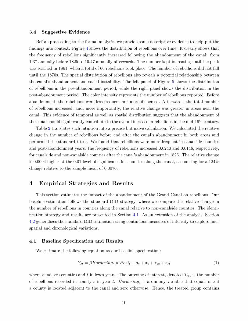
3.4 Suggestive Evidence

Before proceeding to the formal analysis, we provide some descriptive evidence to help put the

findings into context. Figure 4 shows the distribution of rebellions over time. It clearly shows that

the frequency of rebellions significantly increased following the abandonment of the canal: from

1.37 annually before 1825 to 10.47 annually afterwards. The number kept increasing until the peak

was reached in 1861, when a total of 66 rebellions took place. The number of rebellions did not fall

until the 1870s. The spatial distribution of rebellions also reveals a potential relationship between

the canal’s abandonment and social instability. The left panel of Figure 5 shows the distribution

of rebellions in the pre-abandonment period, while the right panel shows the distribution in the

post-abandonment period. The color intensity represents the number of rebellions reported. Before

abandonment, the rebellions were less frequent but more dispersed. Afterwards, the total number

of rebellions increased, and, more importantly, the relative change was greater in areas near the

canal. This evidence of temporal as well as spatial distribution suggests that the abandonment of

the canal should significantly contribute to the overall increase in rebellions in the mid-19th century.

Table 2 translates such intuition into a precise but naive calculation. We calculated the relative

change in the number of rebellions before and after the canal’s abandonment in both areas and

performed the standard t test. We found that rebellions were more frequent in canalside counties

and post-abandonment years: the frequency of rebellions increased 0.0240 and 0.0146, respectively,

for canalside and non-canalside counties after the canal’s abandonment in 1825. The relative change

is 0.0094 higher at the 0.01 level of significance for counties along the canal, accounting for a 124%

change relative to the sample mean of 0.0076.

4 Empirical Strategies and Results

This section estimates the impact of the abandonment of the Grand Canal on rebellions. Our

baseline estimation follows the standard DID strategy, where we compare the relative change in

the number of rebellions in counties along the canal relative to non-canalside counties. The identi-

fication strategy and results are presented in Section 4.1. As an extension of the analysis, Section

4.2 generalizes the standard DID estimation using continuous measures of intensity to explore finer

spatial and chronological variations.

4.1 Baseline Specification and Results

We estimate the following equation as our baseline specification:

Yct = βBorderingc × Postt + δc + σt + χct + εct (1)

where c indexes counties and t indexes years. The outcome of interest, denoted Yct, is the number

of rebellions recorded in county c in year t. Borderingc is a dummy variable that equals one if

a county is located adjacent to the canal and zero otherwise. Hence, the treated group contains

10

counties that bordered the canal, while the control group contains counties that did not. Postt is

a dummy variable that equals one for the years after the abandonment. The equation also controls

for county and year fixed effects, δi and σt; χct denotes other controls. The coefficient of interest

in equation (1) is β, the estimated impact of the canal’s abandonment on the number of rebellions.

The coefficient is expected to be positive, which would suggest a greater increase in the number of

rebellions in canalside counties.

The results are reported in Table 3, where the dependent variables are the number of rebellions.

All four columns adopted similar model specifications with different sets of controls. In Column

(1), we control for county fixed effects and year fixed effects as the baseline. This allows us to rule

out all time-invariant county features (e.g. location), and year shocks that unanimously affect all

regions (e.g. overall state capacity). Column (2) further includes province-emperor fixed effects to

account for unobservable factors associated with regimes, e.g., policy preferences of the emperors.

Column (3) includes prefecture-specific year trends to account for differences in regional trends.

Column (4) includes all previous controls simultaneously. For each column, the standard errors

reported in the parentheses are clustered at the county level (as reported in parentheses) 7. We

also include Conley standard errors in the square brackets following the approaches suggested in

Conley (1999) and Conley (2008) to adjust for spatial correlations.

The results obtained across all specifications are positive and significant, suggesting a higher

number of rebellions associated with the canal’s abandonment. As an example of interpretation, the

point estimator in Column (1) represents 0.0094 more rebellions experienced by counties bordering

the canal (compared to non-canalside counties) after the reform (relative to before). The effect

corresponds to a 124% increase from the sample mean (0.0076), and is significant at the 95%

confidence interval. The estimated coefficients from Columns (2) to (4) are very close to those in

Column (1) in terms of magnitude as well as levels of significance.

The analysis is replicated in Appendix B using alternative outcome measures to account for

potential measurement issues. First, to reduce the potentially biasing effects of extreme values, we

use binary measures of outcomes, where the dependent variables are coded 1 if there are any cases of

rebellion recorded, and 0 otherwise. The results are reported in Table B2. The estimated coefficients

and standard errors are almost unchanged relative to those in Table 3. Second, Table B3 presents

the results where the rebellions are normalized by population 8. The estimated coefficients across

all specifications suggest an additional 0.0004 rebellions per 10, 000 people. The scale accounts for

a 133% increase relative to the sample mean, which is close to the non-normalized estimates.

7We have also clustered the standard errors at the prefecture level to account for within prefecture correlations.The results are reported in Table B1. The standard errors are much larger, but still significant.

8Prefecture-level population in 1660, 1776, 1820, 1851, 1880, and 1910 is compiled by Cao (2001). For our analysis,we construct annual county population measures assuming even distribution across counties and linear changes overtime.

11

4.2 Generalized Estimates

One limitation of our empirical studies is the lack of well-defined treated and control groups.

In the baseline we use a coarse specification that assumes binary treatment and two time periods,

which may underestimate the true effects. To refine the identification, this section generalizes the

specification by allowing continuous treatment measures across counties and years. We begin by

exploring variations in treatment intensity across counties. We measure intensity both internally

and externally 9. The internal measure exploits variation in the length of the canal within a

county, while the external one measures the distance from the county seat to the canal. For the

time dimension, we use the number of years after the initial reform to account for the gradual

abandonment process. Models that simultaneously allow for extensions in both dimensions are also

estimated.

We start with models with continuous treatment intensity. For the internal measure of intensity,

we conducted a regression analysis on the following specification:

Yct = βLengthc × Postt + δc + σt + χ+ εct (2)

Yct =80∑ι=0

βιPostt × Lengthι + δc + σt + χ+ εct (3)

where Equation (2) assumes a linear function of canal length, while Equation (3) uses a more flexible

specification to estimate a separate coefficient for each length interval. The coefficient β estimated

from Equation (2) represents the relative change in the number of rebellions per kilometer length of

the canal. It is expected to be positive, since the impact of the canal should be greater in counties

containing longer segments. As a further extension, the coefficients βιs in Equation (3) estimate

the treatment effects for each of the 10-km intervals with counties away from the canal (i.e., the

baseline control group) as the reference group. Accordingly, we would expect these estimates to be

increasing with ι’s.

The coefficients estimated from Equation (2) with county, year and province-emperor fixed

effects are reported in Column (2) of Table 4; the first column is taken from Table 3, Column (2)

for comparison. As expected, the estimated coefficient β suggests an increase of 0.0003 rebellions

per kilometer length of the canal, which is significant at the 99% confidence interval. This means

that counties with an additional 25 km of canal experienced a 100% increase in rebellions relative

to the sample mean 10. For further illustration, Figure 6 plots the coefficients along with the 95%

confidence intervals estimated from Equation (3). The coefficients kept increasing with the length

of the canal, but did not reach statistical significance until a length of 40 km. Therefore, counties

that marginally intersect the canal are not statistically different from those away from the canal in

rebellions. In other words, the treatment effects we have observed in the baseline primarily come

9We use the term internal measure to represent intensity measures within the baseline treated group,i.e., countiesalong the canal. External measure refers to variations in intensity among all sample regions.

10For robustness, we also analyzed models in which the length of the canal is normalized by the size of the county(i.e., a density measure). The results, available from the authors, are consistent with our non-normalized estimates.

12

from counties that are intensively treated by the canal.

Alternatively, the external measure of intensity exploits variations in the distance to the canal,

following similar specifications:

Yct = βDistancec × Postt + δc + σt + χ+ εct (4)

Yct =

400∑ρ=0

βρPostt ×Distanceρ + δc + σt + χ+ εct (5)

where Postt is interacted with Distancec, the distance to the canal, and each of the 25-km distance

intervals, respectively 11. The estimated coefficient β from Equation (4) represents the relative

change in rebellions per kilometer away from the canal, which is expected to be negative as the

impact diminishes. Equation (5) estimates the treatment effects for each of the 25-km distance

intervals; counties 400 km away from the canal serve as the reference group. We expect their

estimates to be smaller for intervals with larger distances.

Column (3) of Table 4 presents the estimated coefficients from Equation (4). Consistent with

our expectations, it suggests 0.01 fewer rebellions per 100 km away, which is significant at the 1%

level. Figure 7 plots the estimated coefficients from Equation (5) for each of the distance intervals.

The coefficients keep decreasing, and remain significant within a distance of 150 km. Counties

located more than 150 km from the canal did not experience more rebellions than those that are

farther away. Therefore, we interpret 150 km as the range of the canal’s impact.

Extensions in the time dimension are motivated by the gradual process of the reform. While

the first experiment was launched in 1826, the canal was not officially abandoned until 1901. This

raises concerns about our two-period baseline model with 1826 as the cutoff. Therefore, we extend

our analysis using continuous measures of reform progress:

Yct = βBorderingc × PostY earst + δc + σt + χ+ εct (6)

Yct =60∑

τ=−40βτBorderingc × Periodτ + δc + σt + χ+ εct (7)

where the treatment indicator is interacted with PostY earst, the number of years after the initial

reform. As such, a later year represents a higher degree of reform completion. The result is

reported in Column (4) of Table 4 with all previous controls. The estimated coefficient β measures

the difference in the slopes of post-reform trends. The difference between treated and control

counties per decade later is 0.001 larger, suggesting yearly expanding trends. Figure 8 plots the

coefficients of Equation (7) to estimate the treatment effects by decade. The pre-reform pattern

unveiled in the figure verifies the common trends assumption, which is critical in a DID context.

The close-to-zero and insignificant estimated coefficients in the pre-periods suggest no evidence for

11Distance is measured from the county seat to the canal. The results are robust to using the least distancebetween county boundary and the canal as well (available upon request).

13

diverging trends prior to the reform. This establishes the validity of our DID design. Meanwhile,

the figure reveals the rebelling dynamics after the implementation of the reform. The canal’s impact

on rebellions arose immediately after 1826 and kept increasing over the next 30 years. After that

the gap between the two groups started to converge, yet remained significant at the 5% level. This

justifies our choice of 1826 as the cutoff.

An alternative measure of the progress of the reform is the amount of grain shipped via the

canal: a smaller amount represents a higher intensity. However, the shipping data is only available

for some of the years between 1724 and 1849 and is very noisy. Nevertheless, we estimate the

treatment effects using the amount of grain shipped to proxy for reform progress and summarize

the results in Table B4. The first column estimates the treatment effects using the actual amount

of grain shipped, while the following two columns use the amount simulated with moving-average

and four-degree polynomials, respectively. The results are consistent with our expectation that a

smaller amount of grain shipped is associated with more canalside rebellions.

Finally, we combine Equation (2) and Equation (6) to allow continuous treatment intensity

in both dimensions simultaneously. Column (5) is interacted PostY earst with Lengthc, whereas

Column (6) is interacted with Distancec. An intuitive way to interpret the results is to refer to

the relative difference in the post-reform trends. The positive coefficient in Column (5) indicates

a steeper trend in counties with longer stretches of the canal, whereas the negative coefficient in

Column (6) indicates a milder effect in counties farther from the canal. Taken together, the results

in Table 4 reveal that the impact of the abandonment was larger in places that were more intensively

affected by (i.e., closer to) the canal, and diverged over time. This reinforced our baseline findings

that the reform was associated with the subsequent wave of rebellions.

5 Robustness

5.1 Including More Controls

To address concerns that our results suffer from omitted variable bias — i.e., that other fac-

tors affecting social conflict may also be correlated with the canal — we include several controls

associated with conflict in the literature.

Section 3.3 summarized the choice and sources of the control variables. We included time-

variant variables like climate shocks directly into our model, and interacted time-invariant variables

( such as terrain ruggedness) with the post-reform indicator to account for potential structural

changes. The results are reported in Table 5. Columns (1) – (8) add the set of controls one at

a time, while Column (9) includes all of them simultaneously. Our main coefficient of interest,

Borderingc×Postt, preserves its significance across all specifications. The magnitude of the effects

is also stable. It ranges from 0.0075 to 0.0100, around 100% to 144% of the sample mean.

As for the control variables, the correlations discovered in our data are consistent with the

conflict literature. For example, extreme weather, in all sorts of measures, is associated with a

higher rate of rebellions. Land ruggedness, however, reduced the frequency of rebellions during

14

the post-reform periods 12. Distance to the Yellow River also contributed to the rise of rebellions,

as suggested by the historical context, yet it does not negate the effects of the canal. We find no

evidence that agricultural technology or culture plays a significant role in our context.

5.2 Truncated Sample Periods

Another threat to our identification strategy is the relatively long sample periods after the

reform. While the launching of the reform in 1826 was not due to previous conflict around the canal,

the social unrest that took place afterwards might reinforce and accelerate the reform process in

subsequent years, raising concerns about reverse causality in later periods 13. Therefore we restrict

our analysis to truncated sample periods to mitigate the potential biasing effects.

Figure 9 depicts the estimated coefficients and 95% confidence intervals from Equation (1) based

on various sample periods. The x-axis labels the last year included in the analysis. The first sample

contains all years prior to 1840, while every subsequent one adds another 10 years. The estimated

coefficients are positive and significant across all samples, suggesting that our analysis is robust

to excluding potentially endogenous periods. Specifically, the estimates from the pre-1840 sample

represent the effects of the reform in the first 25 years, which provides the finest identification.

However, we interpret its coefficient as a lower bound since the reform was in its initial stage

during this period.

5.3 Falsification Test

Because the number of treated observations is relatively small in our sample (73 out of 575),

there might be concerns of spurious correlations due to noise. To address this concern, we compare

the treatment effects we have estimated to the distribution of placebo treatment effects when county

locations are randomly assigned. Specifically, we randomly assign counties to the polygons in our

sample map representing county locations, without replacement. Thus the number of placebo

counties bordering the canal was the same as the number of actual counties, but the selection of

counties was random. Then we estimated the placebo treatment effects using Equation (1) and

compare them to those in Column (1), Table 3.

Figure 10 plots the distribution of t-statistics from the placebo treatment effects for 1, 000,

3, 000, 5, 000 and 10, 000 times. The vertical lines mark the location of the t-statistic of the actual

treatment effect (as in Column (1), Table 3). The share of the placebo t-statistics that is larger

than the actual statistic (P (t ≤ T )) can be interpreted as analogous to a p-value. It suggests the

probability that a randomly assigned treated group will present an effect at the same or higher

level of significance as the actual treated group. As such, we can reject the null that our result is

indifferent to the placebo treatment effects at about the 1% level of significance.

12This is consistent with the findings in Nunn and Puga (2012) that terrain ruggedness benefited African countriesby avoiding the slave trade.

13For instance, the capture of Jiangning (now Nanking) by the Taiping Rebellion in 1853 is believed to acceleratethe reform by many historians as it blocked the source of grain transportation.

15

6 Discussion of Mechanisms

In previous sections we presented evidence that relates the abandonment of the Grand Canal

to the subsequent emergence of rebellions. Now we discuss the mechanisms behind this correlation.

The conflict literature has highlighted two distinct mechanisms that may explain our findings.

First, the reform might have reduced state capacity, and hence increased the probability that the

rebels would win (Besley and Persson, 2010, 2011; Michalopoulos and Papaioannou, 2013). Second,

it might have lowered the opportunity cost, and thus increased the relative benefit, if it succeeded

(Becker, 1968, 1974; Ehrlich, 1973; Hirshleifer, 1995; Grossman, 1991; Acemoglu and Robinson,

2001). Either way, the reform would increase the expected payoff of participating in rebellions

and hence produce instability. In this section, we compare the relative explanatory power of the

alternative mechanisms by testing the validity of their predictions.

6.1 Decline in State Capacity

While county-level measures of state capacity are not available in our data, we employ two

indirect approaches to examine the role of state capacity. The first approach explores variations in

the importance of political control. If state capacity is the primary driving force behind our results,

we would expect a stronger effect in regions that are more important to the government. Therefore

we interact our treatment indicator with two measures of importance — the number of imperial

soldiers assigned and the presence of prefectural capitals. The results are reported in the first two

columns of Table 6. The importance of political control, measured either way, does not exhibit

a higher rate of rebellion in the post-reform period. Furthermore, we find no evidence that the

reform produced more rebellions in regions that are more important to the government (suggested

by the triple interaction terms). The insignificance of these estimates suggests that state capacity

played a very limited (if any) role in these rebellions.

The second approach is to check the placebo effect on other types of social unrest that are

closely related to a decline in state capacity. Specifically, we test the impact of the abandonment

on the frequency of being attacked or retreated into by enemies, based on the rationale that weak

counties are vulnerable to attack and secure to retreat into. If abandoning the canal reduced state

capacity more dramatically in counties it passed through than in others, we should also expect

increases in their chances of being attacked or retreated into. The results are summarized in the

next two columns of Table 6. Column (3) tests the placebo treatment effect on the frequency

of being attacked, whereas Column (4) tests the placebo treatment effect on the frequency that

defeated enemies retreated into the county. Both coefficients are relatively small compared to the

sample mean, and are not significantly different from zero. Thus while the abandonment of the

canal increased the local onset of rebellions, there is no evidence of increases in any other types.

Therefore, the data does not support the decline of state capacity as a potential mechanism.

16

6.2 Reduction of Opportunity Costs

An alternative hypothesis is that the reform might have triggered rebellions by reducing the

rebels’ opportunity costs. In rural sectors, this could happen if abandoning the canal adversely

affected agricultural productivity. In urban areas, where people worked in commercial sectors, re-

bellions could have been induced by the decline in trade accessibility. We examine both possibilities

in this section.

We first check, both directly and indirectly, whether abandoning the canal induced rebellions

because it reduced agricultural productivity. The direct approach exploits variation in grain prices

compiled by Chen and Kung (2016). If agricultural productivity deteriorated after the canal was

abandoned, we would observe inflation in grain prices. The first column of Table 7 regresses grain

prices on the abandonment of the canal. The positive but insignificant estimated coefficient suggests

little evidence that grain price inflation was associated with the reform. As an indirect test, the

next two columns examine whether the impact of the reform was stronger in agricultural regions.

We multiply the baseline interaction with the suitability indicator for wheat and wetland rice, the

two main crops in our sample area (Talhelm et al., 2014). While the main effects of the reform

remain significant, we find no heterogeneity across various levels of crop suitability. Therefore, the

deterioration in agricultural productivity was not supported by the data.

We next turn to the urban sector, where we discovered considerable evidence to support the

channel of declined trade. The first piece of evidence comes from the underdevelopment of local

markets around the canal. In the first column of Table 8, we regress the number of towns and

markets reported in 1820 and 1911 on the reform. The relative change was significantly lower in

regions that were more intensively affected by the canal. This reveals that the reform had strong

adverse impacts on the development of the local market. Second, we find that the impact of the

reform was stronger in more urbanized regions. To see this, we multiply our baseline interaction

by the share of urban areas in 1776 and summarize the result in the second column of Table 8.

In this specification, the baseline interaction Canal × Post represents the treatment effect in the

absence of urbanization, while the triple interaction Canal×Post×1776 Urbanshare estimates the

upward trend as urbanization increased. The result suggests that the impact of the reform was not

present in rural areas, and was stronger in highly urbanized regions. The final test compares the

impact of the reform in places with and without alternative trade routes. Specifically, we interact

the reform indicator with the county’s access to courier roads, the major routes for north-south

transportation by land. In Column (3) of Table 8, the interaction between Canal×Post estimates

the treatment effects for canalside counties without access to the courier roads, while the triple

interaction represents the relative change in the treatment effects in counties with such access. We

observe from the estimated coefficients that access to alternative trade routes offset half of the

impact induced by the reform. 14 In summary, this evidence is consistent with the channel of

14We also verified the canal’s role in mitigating risk, the role that trade usually plays in the course of climateshocks, as suggested by Dube and Vargas (2013). Consistent with their argument, we find that the canal helpedreduce conflict during extreme weather, but such effect was absent after its abandonment. The results are availableupon request.

17

declined access to trade which reduced rebels’ opportunity cost in urban sectors 15.

6.3 Discussion

Our finding that the reform triggered rebellions in urban areas has significant implications.

Unlike their rural counterparts, the labor force in densely populated urban areas has more collective

consciousness and organized politics. During the era of canal transportation, the grain transport

boatmen formed various societies and associations all over the canal 16. Where there was a lack of

socio-economic opportunities, such organizations were likely to transform into gangs, and become

a long-lasting hotbed of secret societies and organized violence. This transformation, while not

well documented in the conflict literature, is consistent with the evolution of gangsters in Chicago

(Haller, 1971), the rise of the mafia in New York city (Critchley, 2008), and many other violent

events around the world.

We further explore this idea using three cross-sectional exercises 17. The first exploits variation

in the emergence of the Green Gang, one of China’s largest and most powerful organized crime

groups in the early 20th century. We obtained a list of Green Gang high-ranking members and

correlated their distribution with the location of the canal. The results, presented in the first

column of Table 9, demonstrate a high concentration around the canal. The second evaluation

regards the rise of communism in southern China during the 1920s. We compiled the year when

the first Communist Party group was founded for each county in Anhui, Jiangsu and Zhejiang, the

provinces with the earliest communist activities in our sample. Column (2) of Table 9 presents

the correlations between the canal and the spread of communism. On average, the Communist

Party emerged earlier in counties that were more intensively affected by the canal. Finally, Column

(3) of Table 9 estimates the correlation between the canal’s intensity and the presence of armed

conflict (with deaths > 0) in the 5 five years after the onset of the Chinese Cultural Revolution

(1966 – 71) 18. It shows that the regions around the canal experienced much more violence than

the others during Cultural Revolution 19. All these results, while not necessarily causal, suggest

that pre-reform labor organizations in urban regions transformed into gangs, secret societies and

organized violence as a result of the reform.

15An alternative interpretation of our findings on urban areas is that they reflect some sort of political grievance(blaming the government for the abandonment) rather than a decline in opportunity costs. To account for thispossibility, we identify a set of regions that experienced mass killing when the Qing military took over their territoryin the 1640s. We would expect stronger effects at the site of mass killing if the impact we have observed is due to suchgrievances. The result, while not reported, is inconsistent with this argument. We do not find a significant differencebetween places with and without a history of mass killing.

16According to historical records, these associations took control of tens of thousands of grain junks and over50, 000 registered members by the late 18th century.

17In all analyses, we restrict our sample to counties within 150km from the canal, the effective regions accordingto our estimation in Section 4.2.

18We thank Andrew Walder for generously sharing his data.19Walder (2014) estimated that the political upheaval resulted in 1.1 to 1.6 million deaths and 22 to 30 million

direct victims of political persecution

18

7 Conclusion

In this paper, we use the abandonment of China’s Grand Canal as a natural experiment to

study the link between economic shocks and social conflicts. This setting is ideal for our research

purpose because the reform was generally unexpected, and was driven by political rather than

economic considerations. Using a dataset covering 575 counties from 1650 to 1911, we find that

the negative economic shock generated significant social instability: compared to counties away

from the canal, counties bordering the canal on average experienced 0.0094 more rebellions after

the canal’s abandonment. The effect represents a 124% increase relative to the sample mean, and

is significant at the 95% confidence interval. Extensions to the specification further show that

the effects spread over a range of 150 km, and kept increasing over the next 30 years. We found

considerable evidence to support our opportunity cost hypothesis. In particular, the increase in

rebellions in counties bordering the canal seems to have been due to the interruption of trade

in urban sectors. We briefly discuss the possible implications for the underlying social structure

in urban regions, and tentatively attempt to relate this to the evolution of organized crime and

communism in the early 20th century.

This paper makes a significant contribution to the conflict literature by examining a permanent

shock to the urban sector that was initiated by the government. Given that the existing literature

primarily focuses on shocks associated with commodity prices and weather volatility, our study

broadens the set of causal evidence that links economic shocks to violent conflict. It can also be

linked to the impact of transportation infrastructure, the persistence of historical events, and the

wave of social unrest in historical China.

19

References

Daron Acemoglu and James A Robinson. A Theory of Political Transitions. American EconomicReview, pages 938–963, 2001.

Ajay Agrawal, Alberto Galasso, and Alexander Oettl. Roads and Innovation. The Review ofEconomics and Statistics, 99(3):417–434, 2017. doi: 10.1162/REST\ a\ 00619.

Joshua D Angrist and Adriana D Kugler. Rural Windfall or a New Resource curse? Coca, Income,and Civil Conflict in Colombia. The Review of Economics and Statistics, 90(2):191–215, 2008.

Cemal Eren Arbatli, Quamrul Ashraf, and Oded Galor. The Nature of Civil Conflict. (2013-15),2015.

Quamrul Ashraf and Oded Galor. The “Out of Africa” Hypothesis, Human Genetic Diversity, andComparative Economic Development. American Economic Review, 103(1):1–46, February 2013.

Jeremy Atack, Michael R Haines, and Robert A Margo. Railroads and the Rise of the Factory: Ev-idence for the United States, 1850-70. Technical report, National Bureau of Economic Research,2008.

Jeremy Atack, Fred Bateman, Michael Haines, and Robert A Margo. Did Railroads Induce orFollow Economic Growth. Social Science History, 34(2):171–97, 2010.

Ying Bai and Ruixue Jia. Elite Recruitment and Political Stability: The Impact of the Abolitionof Chinas Civil Service Exam. Econometrica, 2016.

Ying Bai and James Kai-sing Kung. Climate Shocks and Sino-nomadic Conflict. Review of Eco-nomics and Statistics, 93(3):970–981, 2011.

Nathaniel Baum-Snow. Did Highways Cause Suburbanization? The Quarterly Journal of Eco-nomics, pages 775–805, 2007.

Samuel Bazzi and Christopher Blattman. Economic Shocks and Conflict: Evidence from Commod-ity Prices. American Economic Journal: Macroeconomics, 6(4):1–38, 2014.

Gary S Becker. Crime and Punishment: An Economic Approach. Journal of Political Economy,76(2), 1968.

Gary S Becker. Crime and Punishment: An Economic Approach, pages 1–54. UMI, 1974.

John Bellows and Edward Miguel. War and Local Collective Action in Sierra Leone. Journal ofPublic Economics, 93(11):1144–1157, 2009.

Timothy Besley and Torsten Persson. State Capacity, Conflict, and Development. Econometrica,78(1):1–34, 2010.

Timothy Besley and Torsten Persson. The Logic of Political Violence. The Quarterly Journal ofEconomics, page qjr025, 2011.

Timothy J Besley and Torsten Persson. The Incidence of Civil War: Theory and Evidence. Technicalreport, National Bureau of Economic Research, 2008.

20

Christopher Blattman and Edward Miguel. Civil War. Journal of Economic Literature, 48(1):3–57,2010.

Markus Brckner and Antonio Ciccone. International Commodity Prices, Growth and the Outbreakof Civil War in Sub-Saharan Africa. The Economic Journal, 120(544):519–534, 2010.

Halvard Buhaug and Jan Ketil Rød. Local Determinants of African Civil Wars, 1970C2001. PoliticalGeography, 25(3):315–335, 2006.

Robin Burgess and Dave Donaldson. Can Openness Mitigate the Effects of Weather Shocks?Evidence from India’s Famine Era. The American Economic Review, pages 449–453, 2010.

Marshall Burke, Solomon M. Hsiang, and Edward Miguel. Climate and Conflict. Annual Reviewof Economics, 7(1), 2015.

Marshall B. Burke, Edward Miguel, Shanker Satyanath, John A. Dykema, and David B. Lobell.Warming Increases the Risk of Civil War in Africa. Proceedings of the National Academy ofSciences, 106(49):20670–20674, 2009.

Shuji Cao. The Population History of China, volume 5. Fudan University Press, Shanghai, 2001.

Qiang Chen. Climate Shocks, State Capacity and Peasant Uprisings in North China during 25C1911CE. Economica, 82(326):295–318, 2015.

Shuo Chen and James Kai-sing Kung. Of Maize and Men: the Effect of a New World Crop onPopulation and Economic Growth in China. Journal of Economic Growth, 21(1):71–99, 2016.

Ting Chen, James Kai-sing Kung, and Chicheng Ma. Long Live Keju! The Persistent Effects ofChina’s Imperial Examination System. 2017.

Sui-wai Cheung. Construction of the Grand Canal and Improvement in Transportation in LateImperial China. Asian Social Science, 4(6):p11, 2009.

C. Chi. Key Economic Areas in Chinese History as Revealed in the Development of Public Worksfor Water-control. A. M. Kelley, 1936.

Antonio Ciccone. Transitory Economic Shocks and Civil Conflict. 2008.

Paul Collier and Anke Hoeffler. On Economic Causes of Civil War. Oxford economic papers, 50(4):563–573, 1998.

Paul Collier and Anke Hoeffler. Greed and Grievance in Civil War. Oxford economic papers, 56(4):563–595, 2004.

T. G. Conley. GMM Estimation with Cross Sectional Dependence. Journal of Econometrics, 92(1):1–45, 1999.

Timothy G. Conley. Spatial Econometrics. Palgrave Macmillan, Basingstoke, 2008.

D. Critchley. The Origin of Organized Crime in America: The New York City Mafia, 1891–1931.Routledge Advances in American History. Taylor & Francis, 2008.

Melissa Dell. The Persistent Effects of Peru’s Mining Mita. Econometrica, 78(6):1863–1903, 2010.ISSN 1468-0262. doi: 10.3982/ECTA8121.

21

Simeon Djankov and Marta Reynal Querol. Poverty and Civil War: Revisiting the Evidence. Reviewof Economics and Statistics, 92(4):1035–1041, 2010.

Dave Donaldson. Railroads of the Raj: Estimating the Impact of Transportation Infrastructure.The American Economic Review, forthcoming.

Dave Donaldson and Richard Hornbeck. Railroads and American Economic Growth: a “MarketAccess” Approach. Quarterly Journal of Economics, forthcoming.

Oeindrila Dube and Juan F Vargas. Commodity Price Shocks and Civil Conflict: Evidence fromColombia. The Review of Economic Studies, 80(4):1384–1421, 2013.

Gilles Duranton and Matthew A Turner. Urban Growth and Transportation. The Review ofEconomic Studies, 79(4):1407–1440, 2012.

Isaac Ehrlich. Participation in Illegitimate Activities: A Theoretical and Empirical Investigation.The Journal of Political Economy, pages 521–565, 1973.

M. Elvin. The Pattern of the Chinese Past: A Social and Economic Interpretation. StanfordUniversity Press, 1973.

Joseph Esherick. The Origins of the Boxer Uprising. Univ of California Press, 1988.

James D Fearon and David D Laitin. Ethnicity, Insurgency, and Civil War. American PoliticalScience Review, 97(01):75–90, 2003.

John G Fernald. Roads to Prosperity? Assessing the Link Between Public Capital and Productivity.American Economic Review, pages 619–638, 1999.

Raquel Fernndez and Alessandra Fogli. Culture: An Empirical Investigation of Beliefs, Work,and Fertility. American Economic Journal: Macroeconomics, 1(1):146–77, January 2009. doi:10.1257/mac.1.1.146.

Robert William Fogel. Notes on the Social Saving Controversy. The Journal of Economic History,39(01):1–54, 1979.

Robert William Fogel. Railroads and American economic growth. Cambridge Univ Press, 1994.

Oded Galor and Marc Klemp. Roots of Autocracy. (2015-7), 2017.

D. Gandar. Le Canal Imperial: Etude Historique et Descriptive. Kraus Reprint, 1894.

Pauline Grosjean. A History of Violence: The Culture of Honor and Homicide in the US South.Journal of the European Economic Association, 12(5):1285–1316, 2014. ISSN 1542-4774. doi:10.1111/jeea.12096.

Herschell I Grossman. A General Equilibrium Model of Insurrections. The American EconomicReview, pages 912–921, 1991.

John M Hagedorn and Perry Macon. People and Folks. Gangs, Crime and the Underclass in aRustbelt City. ERIC, 1988.

Michael R Haines and Robert A Margo. Railroads and Local Economic Development: The UnitedStates in the 1850s. Technical report, National Bureau of Economic Research, 2006.

22

Mark H. Haller. Organized Crime in Urban Society: Chicago in the Twentieth Century. Journalof Social History, 5(2):210–234, 1971.

Hφvard Hegre and Nicholas Sambanis. Sensitivity Analysis of Empirical Results on Civil WarOnset. Journal of Conflict Resolution, 50(4):508–535, 2006.

Harold C. Hinton. The Grain Tribute System of the Ch’ing Dynasty. The Far Eastern Quarterly,11(3):339–354, 1952.

Jack Hirshleifer. Anarchy and Its Breakdown. Journal of Political Economy, pages 26–52, 1995.

Solomon M Hsiang, Kyle C Meng, and Mark A Cane. Civil Conflicts are Associated With theGlobal Climate. Nature, 476(7361):438–441, 2011.

Solomon M. Hsiang, Marshall Burke, and Edward Miguel. Quantifying the Influence of Climate onHuman Conflict. Science, 341(6151), 2013.

H. Huang. The Land Tax in China. Columbia university, 1918.

A.W. Hummel. Eminent Chinese of the Ch’ing Period: 1644-1912. SMC publ., 1991.

Macartan Humphreys. Natural Resources, Conflict, and Conflict Resolution Uncovering the Mech-anisms. Journal of Conflict Resolution, 49(4):508–537, 2005.

Murat Iyigun, Nathan Nunn, and Nancy Qian. The Long-run Effects of Agricultural Productivityon Conflict, 1400-1900. 2015.

Murat Iyigun, Nathan Nunn, and Nancy Qian. Winter is Coming: The Long-Run Effects of ClimateChange on Conflict, 1400-1900. (23033), January 2017.

Thorsten Janus and Daniel Riera-Crichton. Economic Shocks, Civil War and Ethnicity. Journalof Development Economics, 115:32–44, 2015.

Saumitra Jha. Trade, Institutions, and Ethnic Tolerance: Evidence from South Asia. AmericanPolitical Science Review, 107(4):806C832, 2013. doi: 10.1017/S0003055413000464.

Ruixue Jia. Weather Shocks, Sweet Potatoes and Peasant Revolts in Historical China. The Eco-nomic Journal, 124(575):92–118, 2014.

James Kai-sing Kung and Chicheng Ma. Autarky and the rise and fall of piracy in Ming China.The Journal of Economic History, 74(02):509–534, 2014a.

James Kai-sing Kung and Chicheng Ma. Can Cultural Norms Reduce Conflicts? Confucianism andPeasant Rebellions in Qing China. Journal of Development Economics, 111(0):132–149, 2014b.

David D Laitin. Nations, States, and Violence. OUP Oxford, 2007.

Jane Kate Leonard. ’Controlling from Afar’ Open Communications and the Tao-Kuang Emperor’sControl of Grand Canal-Grain Transport Management, 1824-26. Modern Asian Studies, 22(4):665–699, 1988.

Ergang Luo. Lu ying bing zhi (Book of the Green Standard Army). Zhonghua Shuju, 1984.

23

Michael E Mann, Zhihua Zhang, Scott Rutherford, Raymond S Bradley, Malcolm K Hughes, DrewShindell, Caspar Ammann, Greg Faluvegi, and Fenbiao Ni. Global Signatures and DynamicalOrigins of the Little Ice Age and Medieval Climate Anomaly. Science, 326(5957):1256–1260,2009.

B.G. Martin. The Shanghai Green Gang: Politics and Organized Crime, 1919-1937. University ofCalifornia Press, 1996.

Halvor Mehlum, Edward Miguel, and Ragnar Torvik. Poverty and Crime in 19th Century Germany.Journal of Urban Economics, 59(3):370–388, 2006.

Guy Michaels. The Effect of Trade on the Demand for Skill: Evidence from the Interstate HighwaySystem. The Review of Economics and Statistics, 90(4):683–701, 2008.

Stelios Michalopoulos and Elias Papaioannou. Pre-Colonial Ethnic Institutions and ContemporaryAfrican Development. Econometrica, 81(1):113–152, 2013.

Edward Miguel. Poverty and Witch Killing. The Review of Economic Studies, 72(4):1153–1172,2005.

Edward Miguel. Poverty and Violence: An Overview of Recent Research and Implications forForeign Aid. Brookings Institution Press, 2007.

Edward Miguel and Shanker Satyanath. Re-examining Economic Shocks and Civil Conflict. Amer-ican Economic Journal: Applied Economics, 3(4):228–32, 2011.

Edward Miguel, Shanker Satyanath, and Ernest Sergenti. Economic Shocks and Civil Conflict: AnInstrumental Variables Approach. Journal of Political Economy, 112(4):725–753, 2004.

H.B. Morse. The Trade and Administration of China. Longmans, Green and Company, 1913.

Jacob Moscona, Nathan Nunn, and James A. Robinson. Social Structure and Conflict: Evidencefrom Sub-Saharan Africa, 2017.

Yuping Ni. Grain Transportation in the Qing Dynasty and Social Change (Chinese Edition). Shang-hai Bookstore Publishing House, 2005.

Nathan Nunn. The Importance of History for Economic Development. Annual Review of Economics,1(1):65–92, 2009.

Nathan Nunn and Diego Puga. Ruggedness: The Blessing of Bad Geography in Africa. Review ofEconomics and Statistics, 94(1):20–36, 2012.

Nathan Nunn and Leonard Wantchekon. The Slave Trade and the Origins of Mistrust in Africa.American Economic Review, 101(7):3221–3252, 2011.

Elisabeth Ruth Perlman. Dense Enough To Be Brilliant: Patents, Urbanization, and Transportationin Nineteenth Century America. 2016.

Elisabeth Ruth Perlman and Steven Sprick Schuster. Delivering the Vote: The Political Effec-t of Free Mail Delivery in Early Twentieth Century America. Journal of Economic History,forthcoming.

24

Shawn J. Riley, Stephen D. DeGloria, and Robert Elliot. A Terrain Ruggedness Index that Quan-tifies Topographic Heterogeneity. Intermountain Journal of Sciences, 5(1 - 4):23 –27, 1999.

Michael Ross. A Closer Look at Oil, Diamonds, and Civil War. Annu. Rev. Polit. Sci., 9:265–300,2006.

Heather Sarsons. Rainfall and Conflict: A Cautionary Tale. Journal of Development Economics,115(0):62–72, 2015.

Carol H. Shiue. Transport Costs and the Geography of Arbitrage in Eighteenth-CenturyChina. American Economic Review, 92(5):1406–1419, December 2002. doi: 10.1257/000282802762024566.

Kenneth L Sokoloff. Inventive Activity in Early Industrial America: Evidence from Patent Records,1790C1846. The Journal of Economic History, 48(04):813–850, 1988.

Kenneth L. Sokoloff and Stanley L. Engerman. History Lessons: Institutions, Factors Endowments,and Paths of Development in the New World. The Journal of Economic Perspectives, 14(3):217–232, 2000. ISSN 08953309.

US Geological Survey. GTOPO30, 1996.

Guido Tabellini. The Scope of Cooperation: Values and Incentives. The Quarterly Journal ofEconomics, 123(3):905–950, 2008. doi: 10.1162/qjec.2008.123.3.905.

Guido Tabellini. Culture and Institutions: Economic Development in the Regions of Europe.Journal of the European Economic Association, 8(4):677–716, 2010. ISSN 1542-4774. doi: 10.1111/j.1542-4774.2010.tb00537.x.

T Talhelm, X Zhang, S Oishi, C Shimin, D Duan, X Lan, and S Kitayama. Large-scale PsychologicalDifferences within China Explained by Rice versus Wheat Agriculture. Science, 344(6184):603–608, 2014.

Nico Voigtlander and Hans-Joachim Voth. Persecution Perpetuated: The Medieval Origins of Anti-Semitic Violence in Nazi Germany. The Quarterly Journal of Economics, 127(3):1339–1392, 2012.doi: 10.1093/qje/qjs019.

F. Wakeman. The Great Enterprise: The Manchu Reconstruction of Imperial Order in Seventeenth-century China. California University, 1985. ISBN 9780520048041.

Andrew G. Walder. Rebellion and repression in china, 1966c1971. Social Science History, 38(3-4):513C539, 2014. doi: 10.1017/ssh.2015.23.

A.J. Watson. Transport in Transition: the Evolution of Traditional Shipping in China. Michi-gan abstracts of Chinese and Japanese works on Chinese history. Center for Chinese Studies,University of Michigan, 1972. ISBN 9780892649037.

Baojiong Zhu and Peilin Xie, editors. Ming-Qing Jinshi Timing Beilu Suoyin (Official Directoryof Ming-Qing Imperial Exam Graduates). Shanghai: Shanghai Guji Chubanshe, 1980.

25

Figures

Figure 1: Location of the Grand Canal

26

Figure 2: Annual Population Growth at the Prefecture Level

27

Figure 3: Counties Contained in the Sample

28

Figure 4: The Dynamics of Rebellions over Time

29

Figure 5: The Spatial Distribution of Rebellions before and after the Abandonment

30

Figure 6: More Flexible Estimation of the Treatment Effects by Canal Length

31

Figure 7: More Flexible Estimation of the Treatment Effects by Distance to the Canal

32

Figure 8: More Flexible Estimation of the Treatment Effects by Decades

33

Figure 9: Treatment Effects with Gradually Expanding Years of Analysis

34

Figure 10: The Distribution of t-statistics from Randomly Assigned Placebo Treatment Effects

35

Tables

Table 1: Descriptive Statistics

Source Obs. Mean S.D

OutcomesPresence of Rebellions (Onset) 1 150,650 0.0073 0.0854Number of Rebellions (Onset) 1 150,650 0.0076 0.0894

TreatmentsBeing Along the Grand Canal 2 575 0.1270 0.3332Length of Canal within Boundary (km) 2 575 4.1196 13.3217Distance from the Grand Canal (km) 2 575 118.0353 113.4459

ControlsTemperature Deviated from 1961-2006 Mean 3 143,838 -0.1954 0.3343Drought 4 150,650 0.0976 0.2968Flood 4 150,650 0.0743 0.2623Ruggedness Index 5 575 72.7510 97.6787Distance from the Yellow River (km) 2 575 296.8347 267.3429Year of Maize Adoption 4 563 1,718.4050 95.6149Year of Sweet Potato Adoption 4 231 1,755.0130 51.2365jinshi 6 150,650 0.1563 0.8558

SupplementsImperial Soldiers Stationed 7 575 154.2104 345.8505Prefecture Capital 2 575 0.1391 0.3464Number of Attacking Cases 1 150,650 0.0054 0.0822Number of Retreating Cases 1 150,650 0.0036 0.0690Average Grain Price (Liang/KCal) 4 91,110 0.5980 0.1856Suitability Index for Wheat (Irrigation, M Input) 8 575 4,793.0057 1,836.9174Suitability Index for Wetland Rice (Irrigation, M Input) 8 575 3,758.3572 1,231.6994Number of Towns and Local Markets 2 1,150 12.4957 10.76501776 urbanshare 4 563 8.6055 3.7947Along the Qing Courier Routes 2 575 0.2800 0.4494Mass Kill during the Qing Invasion 9 575 0.0226 0.1488Senior Green Gang Members 10 575 0.2435 1.0592Year of First Communist Party Branch 11 569 1,928.2583 5.2102Armed conflict with non-zero death toll, 1966 - 1971 12 569 0.6432 0.4795

Data Sources:

1. Veritable Records of the Qing Emperors (Qing Shilu)2. Harvard Yenching Institution (2007), CHGIS, Version 4.3. Mann et al. (2009)4. Chen and Kung (2016)5. Nunn and Puga (2012)6. Zhu and Xie (1980)7. Luo (1984)8. FAO (2012), GAEZ: http://gaez.fao.org/Main.html#9. Wakeman (1985)

10. Encyclopedia of the Green Gang (Qingbang Tongcao Huihai)11. Local gazettes12. Walder (2014)

36

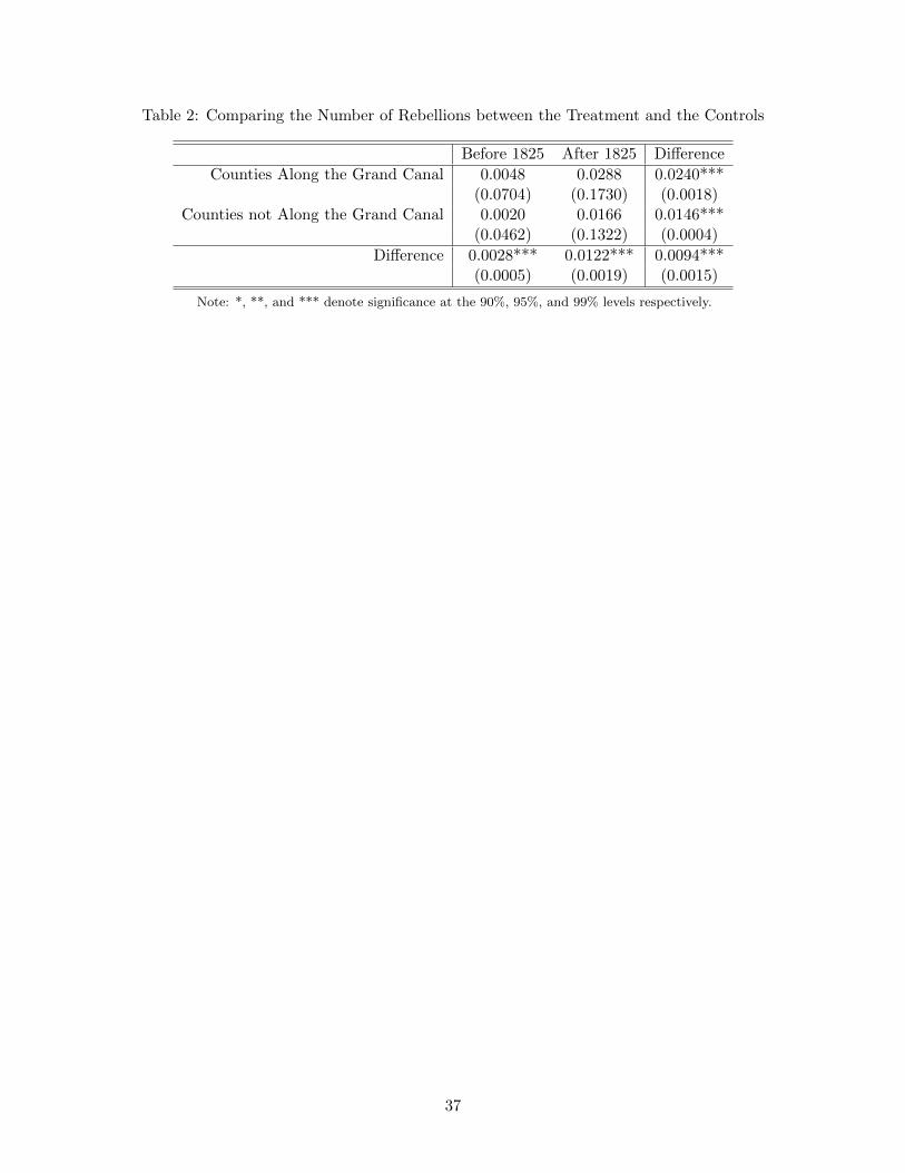
Table 2: Comparing the Number of Rebellions between the Treatment and the Controls

Before 1825 After 1825 Difference

Counties Along the Grand Canal 0.0048 0.0288 0.0240***(0.0704) (0.1730) (0.0018)

Counties not Along the Grand Canal 0.0020 0.0166 0.0146***(0.0462) (0.1322) (0.0004)

Difference 0.0028*** 0.0122*** 0.0094***(0.0005) (0.0019) (0.0015)

Note: *, **, and *** denote significance at the 90%, 95%, and 99% levels respectively.

37

Table 3: The Effects of the Canal’s Abandonment on the Number of Rebellions

Dependent Variable: Number of Rebellions

(1) (2) (3) (4)

Along Canal × After Abandonment 0.0094** 0.0100*** 0.0076** 0.0076**(0.0037) (0.0038) (0.0037) (0.0037)[0.0026] [0.0026] [0.0027] [0.0026]

Constant 0.0119*** -0.0066*** -0.0026 -0.4522**(0.0004) (0.0011) (0.0749) (0.1814)

County FE Yes Yes Yes YesYear FE Yes Yes Yes YesProvince × Emperor FE No Yes No YesPrefecture Year Trend No No Yes Yes

Mean of the Dependent Variable 0.0076 0.0076 0.0076 0.0076No. of Observations 150,650 150,650 150,650 150,650No. of Counties 575 575 575 575No. of Clusters 575 575 575 575Adjusted R-squared 0.0250 0.0263 0.0277 0.0290

Note: *, **, and *** denote significance at the 90%, 95%, and 99% levels, respectively. Standarderrors in parentheses are clustered at the county level. Standard errors in square brackets are Conleystandard errors robust for spatial correlation.

38

Table 4: Continuous Treatment Effects of the Abandonment of the Canal on the Number of Rebellions

Measure of Treatment Intensity: Dependent Variable: Number of Rebellions

(1) (2) (3) (4) (5) (6)

Binary (Baseline):Along Canal × After Abandonment 0.0100***

(0.0038)Continuous intensity:

Canal Length × After Abandonment 0.0034***(0.0013)

Distance to Canal × After Abandonment -0.0005***(0.0001)

Continuous progressAlong Canal × Years after Abandonment 0.0011*

(0.0006)Continuous in both

Canal Length × Years after Abandonment 0.0004**(0.0002)

Distance to the Canal × Years after Abandonment -0.0001***(0.0000)

Constant -0.0066*** -0.0066*** -0.0091*** -0.0066*** -0.0066*** -0.0079***(0.0011) (0.0011) (0.0013) (0.0011) (0.0011) (0.0012)

County FE Yes Yes Yes Yes Yes YesYear FE Yes Yes Yes Yes Yes YesProvince × Emperor FE Yes Yes Yes Yes Yes Yes

Mean of the Dependent Variable 0.0076 0.0076 0.0073 0.0076 0.0076 0.0073No. of Observations 150,650 150,650 139,384 150,650 150,650 139,384No. of Counties 575 575 532 575 575 532No. of Clusters 575 575 532 575 575 532Adjusted R-squared 0.0263 0.0266 0.0265 0.0261 0.0263 0.0262

Note: *, **, and *** denote significance at the 90%, 95%, and 99% levels respectively. Standard errors are clustered at the county level. The length anddistance measures are rescaled to 10 km. Number of years since the reform is measured in decades.

39

Table 5: The Effects of the Canal’s Abandonment with Multiple Controls

Dependent Variable: Number of Rebellions

(1) (2) (3) (4) (5) (6) (7) (8) (9)

Canal × Post 0.0097** 0.0100*** 0.0100*** 0.0076** 0.0091** 0.0099*** 0.0100*** 0.0100*** 0.0075*(0.0038) (0.0038) (0.0037) (0.0038) (0.0038) (0.0038) (0.0037) (0.0038) (0.0039)

Climate:Temperature Deviation 0.0072** 0.0063**

(0.0029) (0.0030)Drought 0.0019** 0.0024***

(0.0009) (0.0009)Flooding 0.0023** 0.0026**

(0.0010) (0.0011)Geography:

Ruggedness × After -0.0000*** -0.0000***(0.0000) (0.0000)

Distance to Yellow River × After -0.0000*** -0.0000**(0.0000) (0.0000)

Technology:Maize Adopted 0.0017 0.0020*

(0.0011) (0.0011)Sweet Potato Adopted -0.0002 -0.0004

(0.0013) (0.0013)Culture:

jinshi 0.0002 0.0003(0.0002) (0.0003)

Constant -0.0042*** -0.0066*** -0.0067*** -0.0002 -0.0045*** -0.0063*** -0.0066*** 0.0125*** 0.0012(0.0014) (0.0011) (0.0011) (0.0012) (0.0010) (0.0012) (0.0011) (0.0011) (0.0022)

County FE Yes Yes Yes Yes Yes Yes Yes Yes YesYear FE Yes Yes Yes Yes Yes Yes Yes Yes YesProvince × Emperor FE Yes Yes Yes Yes Yes Yes Yes Yes Yes

Mean of the Dependent Variable 0.0075 0.0073 0.0073 0.0073 0.0073 0.0074 0.0074 0.0073 0.0077No. of Observations 143,838 150,650 150,650 150,650 150,650 147,506 147,506 150,650 141,218No. of Counties 549 575 575 575 575 563 563 575 539No. of Clusters 549 575 575 575 575 563 563 575 539Adjusted R-squared 0.0274 0.0263 0.0263 0.0266 0.0266 0.0267 0.0267 0.0263 0.0282

Note: *, **, and *** denote significance at the 90%, 95%, and 99% levels respectively. The treatment is measured by along canal indicator.Standard errors are clustered at the county level.

40

Table 6: Testing the Shocks to State Capacity

Dependent Variable:

Baseline Outcome Placebo Outcome

Rebellions (Onset Case) Attack Case Retreat Case

(1) (2) (3) (4)

Canal × Post 0.0003** 0.0003*** 0.0000 0.0000(0.0001) (0.0001) (0.0001) (0.0000)

Soldiers × Post -0.0003(0.0002)

Canal × Post × Soldiers 0.0000(0.0000)

Prefecture Capital × Post 0.0047(0.0029)

Canal × Post × Capital -0.0003(0.0002)

Constant 0.0120*** 0.0123*** 0.0137*** 0.0040***(0.0004) (0.0004) (0.0003) (0.0002)

County FE Yes Yes Yes YesYear FE Yes Yes Yes Yes

Mean of the Dependent Variable 0.0076 0.0073 0.0054 0.0036No. of Observations 150,650 143,052 150,650 150,650No. of Counties 575 546 575 575Adjusted R-squared 0.0253 0.0245 0.0959 0.0785

Note: *, **, and *** denote significance at the 90%, 95%, and 99% levels respectively. The treatment ismeasured by the length of the canal within a county. Standard errors are clustered at the county level.

41

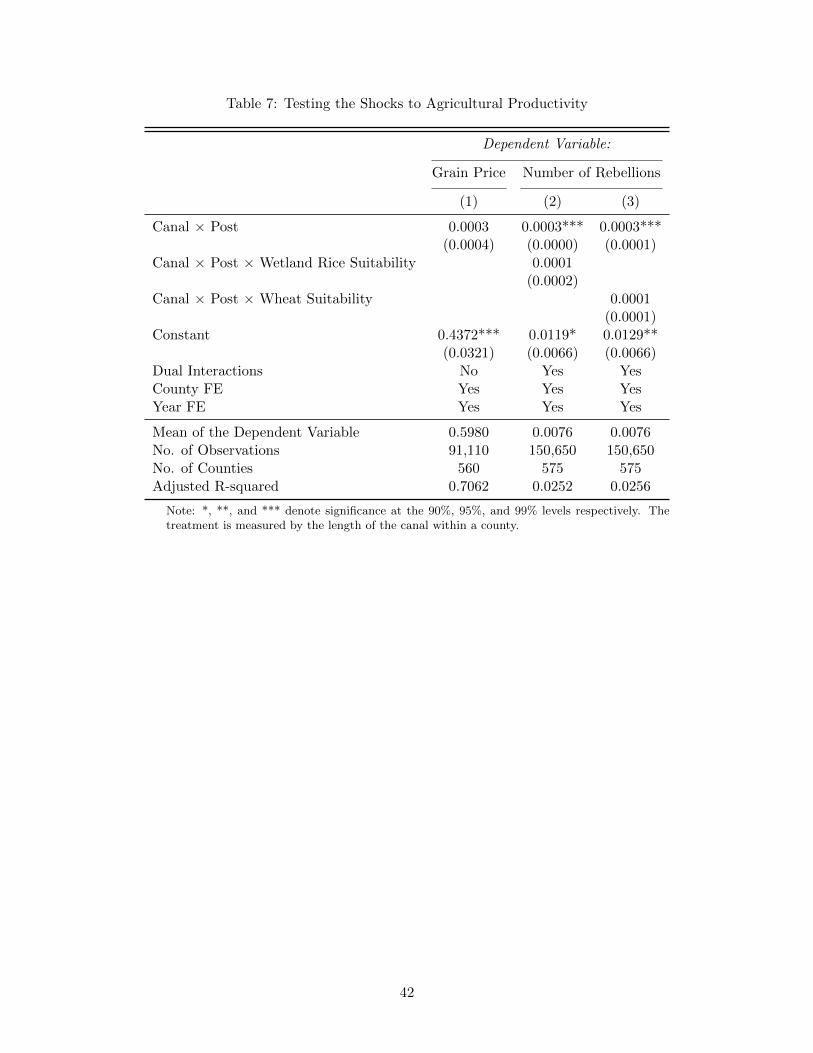
Table 7: Testing the Shocks to Agricultural Productivity

Dependent Variable:

Grain Price Number of Rebellions

(1) (2) (3)

Canal × Post 0.0003 0.0003*** 0.0003***(0.0004) (0.0000) (0.0001)

Canal × Post × Wetland Rice Suitability 0.0001(0.0002)

Canal × Post × Wheat Suitability 0.0001(0.0001)

Constant 0.4372*** 0.0119* 0.0129**(0.0321) (0.0066) (0.0066)

Dual Interactions No Yes YesCounty FE Yes Yes YesYear FE Yes Yes Yes

Mean of the Dependent Variable 0.5980 0.0076 0.0076No. of Observations 91,110 150,650 150,650No. of Counties 560 575 575Adjusted R-squared 0.7062 0.0252 0.0256

Note: *, **, and *** denote significance at the 90%, 95%, and 99% levels respectively. Thetreatment is measured by the length of the canal within a county.

42

Table 8: Testing the Shocks to Trade Accessibility

Dependent Variable:

Town Number Number of Rebellions

(1) (2) (3)

Canal × Post -0.1234*** -0.0023* 0.0028***(0.0389) (0.0012) (0.0006)

Canal × Post × 1776 Urbanshare 0.0004***(0.0001)

Canal × Post × Courier -0.0015**(0.0008)

Constant 1.2222*** 0.0117* 0.0116*(0.0292) (0.0066) (0.0066)

Dual Interactions No Yes YesCounty FE Yes Yes YesYear FE Yes Yes Yes

Mean of the Dependent Variable 2.1228 0.0076 0.0076No. of Observations 1,104 147,506 150,650No. of Counties 575 563 575Adjusted R-squared 0.6523 0.0253 0.0249

Note: *, **, and *** denote significance at the 90%, 95%, and 99% levels respectively.The treatment is measured by the length of canal within the boundary normalized bythe sizes of the counties.

43

Table 9: Testing the Persistent Effects of the Reform

Dependent variable:

Green Gang High-ranking Members Year of Communism Emergence Armed conflict(early 20th century) (1920 – 1949) (1966 – 1971)

(1) (2) (3)

Canal 0.0305*** -0.0327* 0.0027*(0.0098) (0.0189) (0.0015)

Prefecture FE Yes Yes Yes

Mean of the Dependent Variable 0.3533 1926.7339 0.6603No. of Observations 317 109 312Adjusted R-squared 0.1712 0.0597 0.1450

Note: *, **, and *** denote significance at the 90%, 95%, and 99% levels respectively. The treatment is measured by the length of the canalwithin the boundary.

44

A Additional Data Description

A.1 Coding Method

This section summarizes the coding method of our dependent variable: the number of rebellions. We start by

describing the structure and content of Qing Shilu (The Veritable Records of Qing Emperors). Then the detailed

steps taken to locate and code the relevant records are described with illustrative examples.

Qing Shilu is a collection of 13 books (See Figure A1 for a photo of its appearance), each corresponding to one

of the 13 emperors in Qing China. The books consist of the words, orders and activities of the emperors documented

by the court on a daily basis. According to many historians, they provide the most detailed information on social

instability (among many others) throughout the Qing Dynasty.

We collected and digitalized the information in the Qing Shilu in two steps. In the first step, we identified the

items related to rebellions from the books by searching for the keyword “fei” (bandits), which is the most common

term used by the Qing government to refer to rebels 20. We document a separate record for each county mentioned

in the identified items, which gives us 3, 041 mentions of rebellions after dropping the duplications.

In the second step, we categorized the mentions through a close reading of the text. We defined five collectively

exhaustive and mutually exclusive groups of actions taken by the rebels: onset, attacking, defending, stationing and

retreating. Specifically, onset refers to cases where the rebelling group did not exist previously and started to rebel

locally. This is often identified by phases such as “hu you” (suddenly there is), “shu qi” (raise their flag), “qi shi”

(starts rebelling), etc. Attacking refers to cases where the rebelling group already exists and is trying to attack

another county. Defending refers to cases where the rebelling group already exists and is being repressed by the

government. Stationing refers to cases where the rebelling group already exists and is staying in one county without

other military action. Finally, Retreating refers to cases where the rebelling group already exists and is retreating to

a county (often after being defeated by the government).

For illustration, Figure A2 demonstrates a typical record obtained from the Qing Shilu. The report one of the

emperor’s orders in July 1900, saying that a group of rebels formed in Jiangshan County and Pucheng County and

that they have conquered Jiangshan County and Changshan County. In this example, we identify two cases of onset

events in 1900, one in Jiangshan County and the other in Pucheng County. Changshan County, however, is coded

with one attacking event in the data. Our categorization is mutually exclusive in the sense that Jiangshan County is

no longer coded with an attacking event in this record once it has been coded as onset (i.e., it is the place where the

rebellion starts).

The number of rebellions (by category) in each county year is defined as the total number of separate events

in each category 21 . For the purposes of this paper, we restrict our analysis to the cases of local onsets to avoid the

complexity of military considerations. Yet we use the attacking and retreating cases as placebos in the discussion of

mechanisms.

20The Qing government often referred to rebel groups according to their identity (usually the location or theleader’s surname) followed by the keyword “fei”. For example, “yue fei” refers to rebelling groups originating fromGuangdong and Guangxi (also named “yue”); “cuan fei” refers to rebels moving around (“cuan”).

21By the term separate we mean events that are not obviously connected according to the text record. Forexample, if the county reports two onset cases in one year, the number of onset events in that county year will becoded as 2 as long as there is no explicit connection between these two events implied in the text (e.g. one is acontinuation of the other, or initiated by the same leader, or there is some sort of collusion between the rebels, etc.).It is possible that the two events are implicitly connected in an unobservable manner that is not recorded. We addressthis concern by using the presence of rebellion as a robustness check in our analysis.

45

A.Figures

Figure A1: The Photo of Qing Shilu

46

Figure A2: Coding Method

July, Guangxu 26 (1900):

A telegraph report from Shutang Liu suggests that a rebel group led by Laitou Wu and Jiafu Liu has

formed in Jiangshan County and Pucheng County. They have captured Jiangshan County and Chang-

shan County. Keep alert!

Guangxu Shilu (vol. 266)

47

B Supplementary Results

Figure B1: Suitability Index for Wetland Rice (irrigation, medium input)

48

_Zhili

Hubei

Henan

Anhui

Jiangxi

Shandong

Zhejiang

Jiangsu

_ Beijing

The Grand CanalYangtze RiverMain region for grain collectionProvinces Collecting Tribute Grain

Figure B2: Sources and Shipping Routes of tribute rice in the Qing Dynasty

49

Figure B3: Shipping Amount of Grains

50

(a) Across Regions

(b) Over Time

Figure B4: Distribution of Climate Measures

51

Figure B5: Spatial Distribution of the Ruggedness Index

52

(a) Year of Adoption

(b) Number of Counties Adopted

Figure B6: The Spread of New World Crops

53

(a) Across Regions

(b) Over Time

Figure B7: The Distribution of jinshi

54

Table B1: The Effects of the Canal’s Abandonment on the Number of Rebellions Clustered at thePrefecture Level

Dependent Variable: Number of Rebellions

(1) (2) (3) (4)

Along Canal × After Abandonment 0.0094** 0.0100** 0.0076* 0.0076*(0.0044) (0.0040) (0.0042) (0.0040)[0.0026] [0.0026] [0.0027] [0.0026]

Constant 0.0119*** -0.0066*** -0.0026 -0.4522***(0.0007) (0.0020) (0.0290) (0.1576)

County FE Yes Yes Yes YesYear FE Yes Yes Yes YesProvince × Emperor FE No Yes No YesPrefecture Year Trend No No Yes Yes

Mean of the Dependent Variable 0.0076 0.0076 0.0076 0.0076No. of Observations 150,650 150,650 150,650 150,650No. of Counties 575 575 575 575No. of Clusters 79 79 79 79Adjusted R-squared 0.0250 0.0263 0.0277 0.0290

Note: *, **, and *** denote significance at the 90%, 95%, and 99% levels respectively. Standarderrors in parentheses are clustered at the prefecture level. Standard errors in square brackets areConley standard errors robust for spatial correlation.

55

Table B2: The Effects of the Canal’s Abandonment on the Presence of Rebellions

Dependent Variable: Presence of Rebellions

(1) (2) (3) (4)

Along Canal × After Abandonment 0.0090** 0.0097*** 0.0071** 0.0071**(0.0035) (0.0035) (0.0035) (0.0035)[0.0025] [0.0025] [0.0025] [0.0025]

Constant 0.0121*** -0.0062*** -0.0074 -0.4471**(0.0004) (0.0010) (0.0749) (0.1803)

County FE Yes Yes Yes YesYear FE Yes Yes Yes YesProvince × Emperor FE No Yes No YesPrefecture Year Trend No No Yes Yes

Mean of the Dependent Variable 0.0073 0.0073 0.0073 0.0073No. of Observations 150,650 150,650 150,650 150,650No. of Counties 575 575 575 575No. of Clusters 575 575 575 575Adjusted R-squared 0.0239 0.0253 0.0265 0.0278

Note: *, **, and *** denote significance at the 90%, 95%, and 99% levels, respectively. Standarderrors in parentheses are clustered at the county level. Standard errors in square brackets are Conleystandard errors robust for spatial correlation.

56

Table B3: The Effects of the Canal’s Abandonment on Rebellions Normalized by Population

Dependent Variable:Number of Rebellions Presence of Rebellions

(1) (2) (3) (4)

Along Canal × After Abandonment 0.0004* 0.0004** 0.0003* 0.0004**(0.0002) (0.0002) (0.0002) (0.0002)[0.0002] [0.0001] [0.0001] [0.0001]

Constant 0.0001*** -0.0001*** 0.0001*** -0.0001***(0.0000) (0.0000) (0.0000) (0.0000)

County FE Yes Yes Yes YesYear FE Yes Yes Yes YesProvince × Emperor FE No Yes No Yes

Mean of the Dependent Variable 0.0003 0.0003 0.0003 0.0003No. of Observations 129,854 129,854 129,854 129,854No. of Counties 575 575 575 575No. of Clusters 563 563 563 563Adjusted R-squared 0.0145 0.0171 0.0139 0.0165

Note: *, **, and *** denote significance at the 90%, 95%, and 99% levels, respectively. The dependentvariables are normalized by population. Standard errors in parentheses are clustered at the countylevel. Standard errors in square brackets are Conley standard errors robust for spatial correlation.

57

Table B4: Continuous Treatment Effects using the Amount of Grain Shipped via Canal

Dependent Variable: Number of Rebellions

(1) (2) (3)

Canal Length × Shipping Amount (Actual) -0.0017**(0.0008)

Canal Length × Shipping Amount (Moving Average) -0.0005**(0.0002)

Canal Length × Shipping Amount (Simulated) -0.0103***(0.0032)

Constant -0.0033 -0.0077*** -0.0049***(0.0116) (0.0009) (0.0010)

County FE Yes Yes YesYear FE Yes Yes YesProvince × Emperor FE Yes Yes Yes

Mean of the Dependent Variable 0.0055 0.0083 0.0075No. of Observations 25,750 66,950 81,885No. of Counties 515 515 515Adjusted R-squared 0.0111 0.0266 0.0280

Note: *, **, and *** denote significance at the 90%, 95%, and 99% levels respectively. Canal length is measured per10 km, and shipping amount is measured per million dan. Standard errors in Columns (2) and (3) are clustered atthe county level.

58