Robin Hofmann, Leonie Ahrendts, and Rolf Ernst

23CPA: Compositional Performance Analysis

Robin Hofmann, Leonie Ahrendts, and Rolf Ernst

Abstract

In this chapter we review the foundations Compositional Performance Analysis(CPA) and explain many extensions which support its application in designpractice. CPA is widely used in automotive system design where it successfullycomplements or even replaces simulation-based approaches.

Acronyms

ACK AcknowledgementARQ Automatic Repeat RequestBCET Best-Case Execution TimeBCRT Best-Case Response TimeCAN Controller Area NetworkCOTS Commercial/Components Off-The-ShelfCPA Compositional Performance AnalysisDAG Directed Acyclic GraphDMA Direct Memory AccessECU Electronic Control UnitFIFO First-In First-OutMCR Mode Change RequestSPNP Static-Priority Non-PreemptiveSPP Static Priority PreemptiveTWCA Typical Worst-Case AnalysisTWCRT Typical Worst-Case Response TimeWCET Worst-Case Execution TimeWCRT Worst-Case Response Time

R. Hofmann (�) • L. Ahrendts • R. ErnstInstitute of Computer and Network Engineering, Technical University Braunschweig,Braunschweig, Germanye-mail: [email protected]; [email protected]; [email protected]

© Springer Science+Business Media Dordrecht 2017S. Ha, J. Teich (eds.), Handbook of Hardware/Software Codesign,DOI 10.1007/978-94-017-7267-9_24

721

mailto:[email protected]



722 R. Hofmann et al.

Contents

23.1 Motivation . . . . . . . . . . . . . . . . . . . . . . . . . . . . . . . . . . . . . . . . . . . . . . . . . . . . . . . . . . . . . 72223.2 Fundamentals . . . . . . . . . . . . . . . . . . . . . . . . . . . . . . . . . . . . . . . . . . . . . . . . . . . . . . . . . . 723

23.2.1 Timing Model . . . . . . . . . . . . . . . . . . . . . . . . . . . . . . . . . . . . . . . . . . . . . . . . . . . 72423.2.2 Analysis . . . . . . . . . . . . . . . . . . . . . . . . . . . . . . . . . . . . . . . . . . . . . . . . . . . . . . . 730

23.3 Extensions . . . . . . . . . . . . . . . . . . . . . . . . . . . . . . . . . . . . . . . . . . . . . . . . . . . . . . . . . . . . . 74023.3.1 Analysis of Systems with Shared Resources . . . . . . . . . . . . . . . . . . . . . . . . . . 74023.3.2 Analysis of Systems Undergoing Mode Changes . . . . . . . . . . . . . . . . . . . . . . 74223.3.3 Analysis of the Timing Impact of Errors and Error Handling . . . . . . . . . . . . . 74323.3.4 Refined Analysis of Task Chains . . . . . . . . . . . . . . . . . . . . . . . . . . . . . . . . . . . . 74523.3.5 Timing Verification of Weakly-Hard Real-Time Systems . . . . . . . . . . . . . . . . 74723.3.6 Further Contributions . . . . . . . . . . . . . . . . . . . . . . . . . . . . . . . . . . . . . . . . . . . . . 748

23.4 Conclusion . . . . . . . . . . . . . . . . . . . . . . . . . . . . . . . . . . . . . . . . . . . . . . . . . . . . . . . . . . . . 748References . . . . . . . . . . . . . . . . . . . . . . . . . . . . . . . . . . . . . . . . . . . . . . . . . . . . . . . . . . . . . . . . . . 748

23.1 Motivation

Despite the risk of overlooking critical corner cases, design verification is forthe most part based on execution and test using simulation, prototyping, and thefinal system. Formal analysis and verification are typically used in cases whereerrors are particularly expensive or may have catastrophic consequences, such as insafety critical or high availability systems. Such formal methods have considerablyimproved in performance and usability and can be used on a broader scale toimprove design quality, but they must cope with growing hardware and softwarearchitecture complexity.

The situation is similar when we consider system timing verification. Formaltiming analysis methods have been around for decades, starting with early workby Liu and Layland in the 70s [24] which provided schedulability analysis andworst-case response time data for a limited set of task system classes and schedulingstrategies for single processors. In the meantime, there were dramatic improvementsin the scope of considered tasks systems, architectures, and timing models. Oneof the key analysis inputs is the maximum execution time of a task, the Worst-Case Execution Time (WCET), where there has been similar progress [51]. As inthe case of function verification, progress in hardware and software architecturesmade analysis more challenging. In particular the dominant trend focusing Commer-cial/Components Off-The-Shelf (COTS) on average or typical system performancehas impaired system predictability forcing analysis to resort to more conservativemethods (i.e., methods that overestimate the real worst case). While architectureswith higher predictability have been proposed [29,51], design practice currently hasto live with the ongoing trend.

In some respect, efficient formal timing verification is even harder than func-tion verification because of systems integration. Today, a vehicle, an aircraft,a medical device, and even a smartphone integrates many applications sharingthe same network, processors, and run-time environment. This leads to potential

23 CPA: Compositional Performance Analysis 723

timing interference of seemingly unrelated applications. The integrated modulararchitecture (IMA), standardized as ARINC 653 [45] for aircraft design, and evenmore the automotive AUTOSAR standard are perfect examples for such softwarearchitectures. They also stand for different philosophies. While ARINC 653 takesa constructive approach and uses scheduling to obtain application isolation at thecost of resource efficiency, AUTOSAR does not constructively prevent timinginterference, but the related automotive safety standard ISO 26262 requires proofof “freedom from interference” for safety critical applications.

However, even with extensive runs on millions of cases, simulation and pro-totyping remain an investigation of collections of use cases with decreasingexpressiveness for large integrated systems. Therefore, there is a strong incentiveto use formal timing analysis methods at least on the network level. For example,there are formal methods for some protocols such as the automotive Controller AreaNetwork (CAN) bus which is the dominant automotive bus standard today [10].Unfortunately, current automotive systems are not only large but heterogeneouscombining different protocols and scheduling and arbitration strategies. To makethings worse, the component and network technology incrementally develops overtime challenging flexibility and scalability of any formal timing analysis.

In this situation, the introduction of modular timing analysis methods whichsupport composition of analyses for different scheduling and arbitration strategies aswell as different architectures and application systems with a variety of models-of-computation was considered a breakthrough. Today, most automotive manufacturersand many suppliers use formal timing analysis as part of their network development.A corresponding tool, SymTA/S, has been commercialized and is widely used. Theoriginal ideas which led to that tool can be found in [37].

This chapter presents the general concept of the Compositional PerformanceAnalysis (CPA) and extensions of the last couple of years. Since this is an overviewchapter, it stays on the surface to keep readability. For more details, the readeris referred to the large body of related scientific papers covering compositionalperformance analysis and a related approach based on the Real-Time Calculus(RTC) [49].

23.2 Fundamentals

CPA is an analysis framework which serves to formally derive the timing behaviorof embedded real-time systems.

From a hardware perspective, an embedded real-time system consists of aset of interconnected components. These components include communication andcomputation elements as well as sensors and actuators which act as the connection tothe system environment. The interconnected components represent the platform onwhich software applications with real-time requirements are executed. A softwareapplication is composed of tasks, entities of computation, which are distributed overand executed on different components of the system.


The execution order of tasks belonging to one application is constrained, forinstance, the read of a sensor must be performed before the computation of acontrol law and the control of an actuator. Moreover, if several tasks are executedon one component, the tasks have to share the processing service the componentoffers. This has obviously an impact on the timing behavior of each task. As aresult, in order to determine the timing behavior of the system, it is not sufficientto focus on isolated tasks. Apart from the interaction of tasks which are causedby functional dependencies (imposed execution order), nonfunctional dependencies(share of component service) have also to be taken into consideration.

In the following, the system model used for CPA is described, and then thecompositional analysis principle is deduced. Following the above argumentation,CPA structures its system model with respect to three aspects: (1) the individualtasks, (2) the individual components with intra-component (local) dependenciesbetween mapped tasks, and (3) the system platform with inter-component (global)dependencies between mapped tasks. The analysis is structured according to the lo-cal and global aspects, and it is compositional in the sense that the timing propertiesof the system can be conclusively derived from its constituting components.

23.2.1 Timing Model

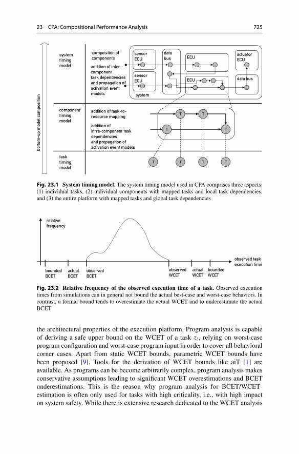
In the following the timing model of a real-time embedded system is described asit is used in CPA. The timing model is layered and includes the task timing model,the component timing model, and the system timing model. All three layers areexplained in detail below and are illustrated in Fig. 23.1.

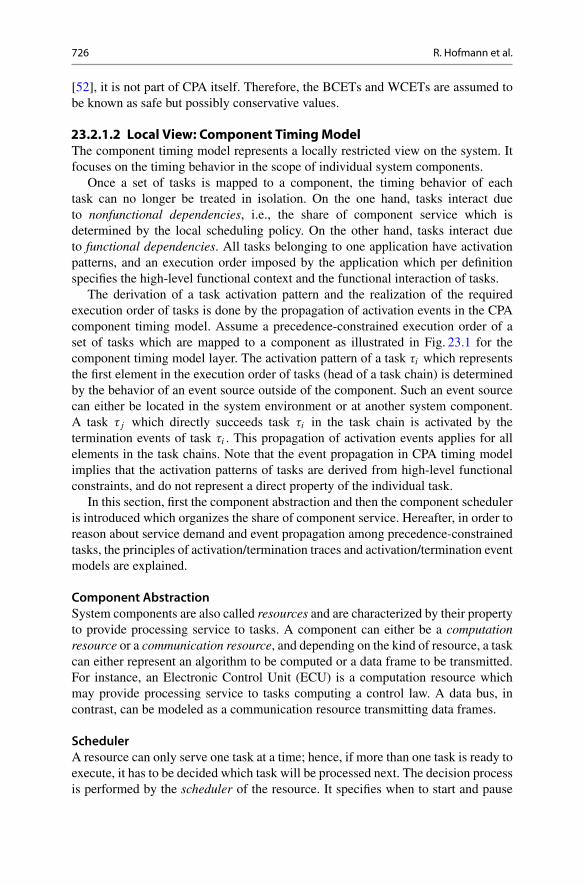
23.2.1.1 Task Timing ModelIn this section the timing behavior of an individual task �i is presented which ischaracterized completely by its execution time Ci . The execution time Ci is theamount of service time which a component has to provide in order to process task �i .The actual execution time of a task �i does not only heavily depend on the task inputand the task state but also on the execution platform. For instance, the processorarchitecture, the cache architecture, and the Direct Memory Access (DMA) policyimpact the execution time. As a result, a task �i does not have a static but rathera varying execution time Ci as illustrated in Fig. 23.2. For the CPA, the lower andthe upper bound on the task execution are of interest because they include everyintermediate timing behavior. The lower bound on the task execution time is calledBest-Case Execution Time (BCET) denoted as C �

i , whereas the upper bound iscalled the WCET denoted as C C

i .Different methods exist to derive the BCET and WCET of a task �i . One

method is to simulate the task execution under different scenarios and observethe required execution time. Since the number of test cases is naturally limited,the simulation is bound not to cover all corner cases thus underestimating theWCET and overestimating the BCET. Formal program analysis, on the other hand,evaluates the source or object code associated with a task �i and takes into account


Fig. 23.1 System timing model. The system timing model used in CPA comprises three aspects:(1) individual tasks, (2) individual components with mapped tasks and local task dependencies,and (3) the entire platform with mapped tasks and global task dependencies

Fig. 23.2 Relative frequency of the observed execution time of a task. Observed executiontimes from simulations can in general not bound the actual best-case and worst-case behaviors. Incontrast, a formal bound tends to overestimate the actual WCET and to underestimate the actualBCET

the architectural properties of the execution platform. Program analysis is capableof deriving a safe upper bound on the WCET of a task �i , relying on worst-caseprogram configuration and worst-case program input in order to cover all behavioralcorner cases. Apart from static WCET bounds, parametric WCET bounds havebeen proposed [9]. Tools for the derivation of WCET bounds like aiT [1] areavailable. As programs can be become arbitrarily complex, program analysis makesconservative assumptions leading to significant WCET overestimations and BCETunderestimations. This is the reason why program analysis for BCET/WCET-estimation is often only used for tasks with high criticality, i.e., with high impacton system safety. While there is extensive research dedicated to the WCET analysis


[52], it is not part of CPA itself. Therefore, the BCETs and WCETs are assumed tobe known as safe but possibly conservative values.

23.2.1.2 Local View: Component Timing ModelThe component timing model represents a locally restricted view on the system. Itfocuses on the timing behavior in the scope of individual system components.

Once a set of tasks is mapped to a component, the timing behavior of eachtask can no longer be treated in isolation. On the one hand, tasks interact dueto nonfunctional dependencies, i.e., the share of component service which isdetermined by the local scheduling policy. On the other hand, tasks interact dueto functional dependencies. All tasks belonging to one application have activationpatterns, and an execution order imposed by the application which per definitionspecifies the high-level functional context and the functional interaction of tasks.

The derivation of a task activation pattern and the realization of the requiredexecution order of tasks is done by the propagation of activation events in the CPAcomponent timing model. Assume a precedence-constrained execution order of aset of tasks which are mapped to a component as illustrated in Fig. 23.1 for thecomponent timing model layer. The activation pattern of a task �i which representsthe first element in the execution order of tasks (head of a task chain) is determinedby the behavior of an event source outside of the component. Such an event sourcecan either be located in the system environment or at another system component.A task �j which directly succeeds task �i in the task chain is activated by thetermination events of task �i . This propagation of activation events applies for allelements in the task chains. Note that the event propagation in CPA timing modelimplies that the activation patterns of tasks are derived from high-level functionalconstraints, and do not represent a direct property of the individual task.

In this section, first the component abstraction and then the component scheduleris introduced which organizes the share of component service. Hereafter, in order toreason about service demand and event propagation among precedence-constrainedtasks, the principles of activation/termination traces and activation/termination eventmodels are explained.

Component AbstractionSystem components are also called resources and are characterized by their propertyto provide processing service to tasks. A component can either be a computationresource or a communication resource, and depending on the kind of resource, a taskcan either represent an algorithm to be computed or a data frame to be transmitted.For instance, an Electronic Control Unit (ECU) is a computation resource whichmay provide processing service to tasks computing a control law. A data bus, incontrast, can be modeled as a communication resource transmitting data frames.

SchedulerA resource can only serve one task at a time; hence, if more than one task is ready toexecute, it has to be decided which task will be processed next. The decision processis performed by the scheduler of the resource. It specifies when to start and pause


the execution of pending tasks. Commonly used scheduling policies for embeddedreal-time systems are Static Priority Preemptive (SPP) and Static-Priority Non-Preemptive (SPNP) scheduling. We will use these policies as important examplesthroughout the chapter, noting that CPA is not limited to static priority policies.

Activation Traces and Termination TracesA task is activated by an activation event, where activation means that the task ismoved from a sleeping state to a ready-to-execute state. Such an activation eventcan either be time triggered or event triggered. A time-triggered activation occursaccording to a predefined time pattern, whereas an event-triggered activation isa reaction to a certain true condition in the system or the system environment.Additionally to being activated by an activation event, a task produces a terminationevent when it has finished.

An activation trace of a task �i describes the set of instants at which an activationevent for a task �i takes place. A similar definition applies to the termination trace.An activation event for a task �i originates either from an event source which istriggered by the system environment or another external event source like a timer,or it is produced by a predecessor task �j if a precedence constraint with respect tothe execution order exists between two tasks in the form of �j ! �i (�j precedes�i ). The termination event of the predecessor task �j , produced at the end of itsexecution, then represents the activation event for task �i . If the predecessor task isnot local to the component, an external event source with a conservative activationpattern is initially assumed in the CPA component timing model, see Sect. 23.2.2.2.

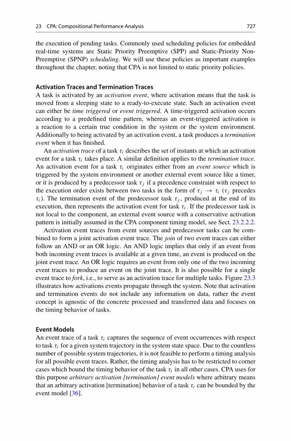
Activation event traces from event sources and predecessor tasks can be com-bined to form a joint activation event trace. The join of two event traces can eitherfollow an AND or an OR logic. An AND logic implies that only if an event fromboth incoming event traces is available at a given time, an event is produced on thejoint event trace. An OR logic requires an event from only one of the two incomingevent traces to produce an event on the joint trace. It is also possible for a singleevent trace to fork, i.e., to serve as an activation trace for multiple tasks. Figure 23.3illustrates how activations events propagate through the system. Note that activationand termination events do not include any information on data, rather the eventconcept is agnostic of the concrete processed and transferred data and focuses onthe timing behavior of tasks.

Event ModelsAn event trace of a task �i captures the sequence of event occurrences with respectto task �i for a given system trajectory in the system state space. Due to the countlessnumber of possible system trajectories, it is not feasible to perform a timing analysisfor all possible event traces. Rather, the timing analysis has to be restricted to cornercases which bound the timing behavior of the task �i in all other cases. CPA uses forthis purpose arbitrary activation [termination] event models where arbitrary meansthat an arbitrary activation [termination] behavior of a task �i can be bounded by theevent model [36].


Fig. 23.3 Event traces. Tasks are activated by activation events from time-triggered or event-triggered event sources as well as by the termination events of predecessor tasks. The arrowsconnecting event sources and tasks as well as tasks among each other indicate the flow of eventsthrough the system. The small arrows # indicate individual activation events which occur regularlyin case of time-triggering and irregularly in case of event-triggering and propagate through thesystem

An event model of a task �i is defined by the set of two distance functionsı�

i ; ıCi W N0 ! R

C0 , namely, the minimum distance function ı�

i and the maximumdistance function ıC

i . The minimum distance function ı�i .n/ describes the minimum

time distance between any n consecutive activation [termination] events of task�i . The maximum distance function ıC

i .n/ describes the maximum time distancebetween any n consecutive activation [termination] events of task �i . The distancebetween zero and one events is defined for mathematical convenience as zero so thatı

C;�i .0/ D ı

C;�i .1/ WD 0.

Pseudo inverses of the distance functions are the arrival functions �Ci ; ��

i W

RC0 ! N0. The maximum arrival function �C

i is the pseudo inverse of the minimumdistance function ı�

i , and the minimum arrival function ��i is the pseudo inverse

of the maximum distance function ıCi . The function �C.�t/, resp. ��.�t/, returns

the maximum, resp. minimum, number of activation [termination] events of task �i

within any half-open time interval Œt; t C �t/. For a time interval �t D 0, theevent arrival functions ��

i and �Ci are defined as zero. The pseudo inverses are

introduced because they often allow a more elegant mathematical formulation oftiming analysis problems.

The pair of minimum and maximum distance functions, resp. arrival functions,describe the best-case and worst-case event trace of a task �i with respect to eventfrequency. If distance functions, resp. arrival functions, cannot be formally derived,it is possible to extract them from measured event traces [17].

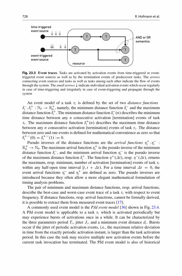
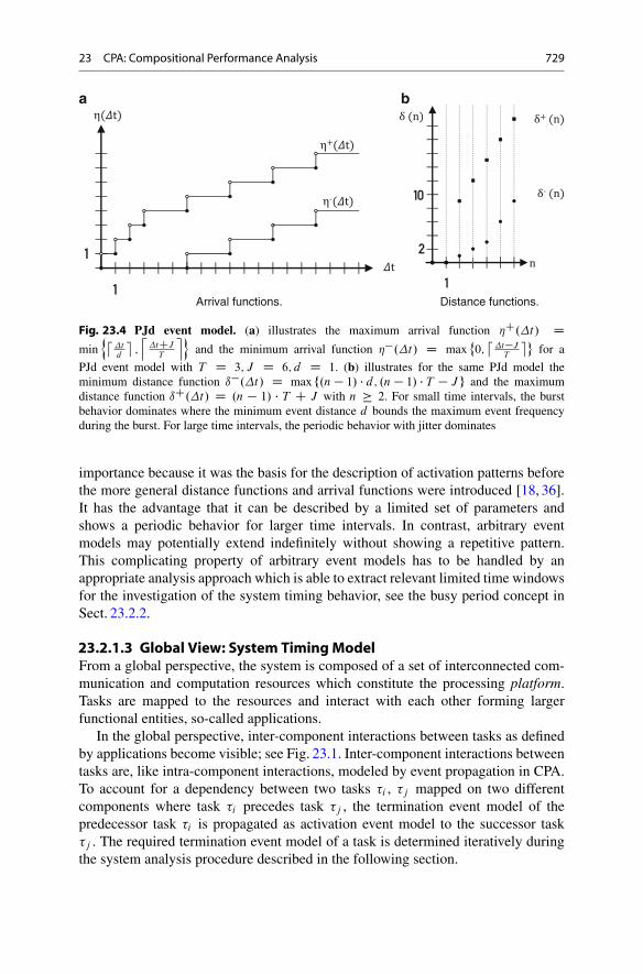
A commonly used event model is the PJd event model [36] shown in Fig. 23.4.A PJd event model is applicable to a task �i which is activated periodically butmay experience bursts of activations once in a while. It can be characterized bythe three parameters period Ti , jitter Ji , and a minimum event distance di . Burstsoccur if the jitter of periodic activation events, i.e., the maximum relative deviationin time from the exactly periodic activation instant, is larger than the task activationperiod. In this case the task may receive multiple new activation events before thecurrent task invocation has terminated. The PJd event model is also of historical


a

Arrival functions. Distance functions.

b

Fig. 23.4 PJd event model. (a) illustrates the maximum arrival function �C.�t/ D

minn˙

�td

�;l

�tCJT

moand the minimum arrival function ��.�t/ D max

˚0;

˙�t�J

T

��for a

PJd event model with T D 3; J D 6; d D 1. (b) illustrates for the same PJd model theminimum distance function ı�.�t/ D max f.n � 1/ � d; .n � 1/ � T � J g and the maximumdistance function ıC.�t/ D .n � 1/ � T C J with n � 2. For small time intervals, the burstbehavior dominates where the minimum event distance d bounds the maximum event frequencyduring the burst. For large time intervals, the periodic behavior with jitter dominates

importance because it was the basis for the description of activation patterns beforethe more general distance functions and arrival functions were introduced [18, 36].It has the advantage that it can be described by a limited set of parameters andshows a periodic behavior for larger time intervals. In contrast, arbitrary eventmodels may potentially extend indefinitely without showing a repetitive pattern.This complicating property of arbitrary event models has to be handled by anappropriate analysis approach which is able to extract relevant limited time windowsfor the investigation of the system timing behavior, see the busy period concept inSect. 23.2.2.

23.2.1.3 Global View: System Timing ModelFrom a global perspective, the system is composed of a set of interconnected com-munication and computation resources which constitute the processing platform.Tasks are mapped to the resources and interact with each other forming largerfunctional entities, so-called applications.

In the global perspective, inter-component interactions between tasks as definedby applications become visible; see Fig. 23.1. Inter-component interactions betweentasks are, like intra-component interactions, modeled by event propagation in CPA.To account for a dependency between two tasks �i , �j mapped on two differentcomponents where task �i precedes task �j , the termination event model of thepredecessor task �i is propagated as activation event model to the successor task�j . The required termination event model of a task is determined iteratively duringthe system analysis procedure described in the following section.


23.2.2 Analysis

CPA is a systematic timing analysis method which serves to verify the timing prop-erties of complex distributed real-time systems with heterogeneous components.The major challenge in analyzing such a system is to take into account the numerousinterdependencies of task executions which result both from direct task interactionand indirect task interaction due to the share of resources.

CPA follows a compositional approach which first performs a local component-related timing verification step and then, in a global timing verification step, sets thelocal verification problems in a system context where inter-component dependenciesare considered. The inter-component dependencies relate the local verificationproblems in such a manner that their inputs and outputs are linked. The relationof the local verification problems leads to a fixed point problem which converges ifthe propagation of outputs to inputs between related verification problems does notchange the verification results any more. If the system is overloaded, the fixed pointproblem does not converge, and an abort criterion, e.g., the detected miss of a taskdeadline, is used to stop the iteration process.

In this section, first the local analysis is presented and then the superordinateglobal analysis is introduced.

23.2.2.1 Local AnalysisLocal analysis refers to the analysis of timing properties of an individual systemresource which processes tasks according to a given scheduling policy. The localanalysis is based on the component timing model.

Resource UtilizationThe utilization U of a resource is defined as the quotient of the execution requestwhich the resource receives and the available service time which it can provide. Itis computed by accumulating the utilization Ui that each task �i with i D 1 : : : N

mapped to this resource imposes. The maximum utilization U Ci that an individual

task �i can impose on a resource is given if the task requests its maximum executiontime C C

i at its maximum activation frequency

U Ci D lim

n!1

n � C Ci

ı�i .n/

: (23.1)

The maximum utilization of a resource U C DPN

iD1 U Ci is an important variable

to determine whether the resource is overloaded, and consequently the tasksare not schedulable. Apparently, it is impossible to schedule tasks sets with aresource utilization larger than one. In this case, the local analysis will be stopped.While being a necessary (under some conditions even sufficient) indicator for theschedulability of a task set, the utilization is not an appropriate means to describethe system timing behavior in detail. The utilization of a resource does not give any


insight into the sequence of execution and suspension phases during the processingof a task which are determined by the applied scheduling policy.

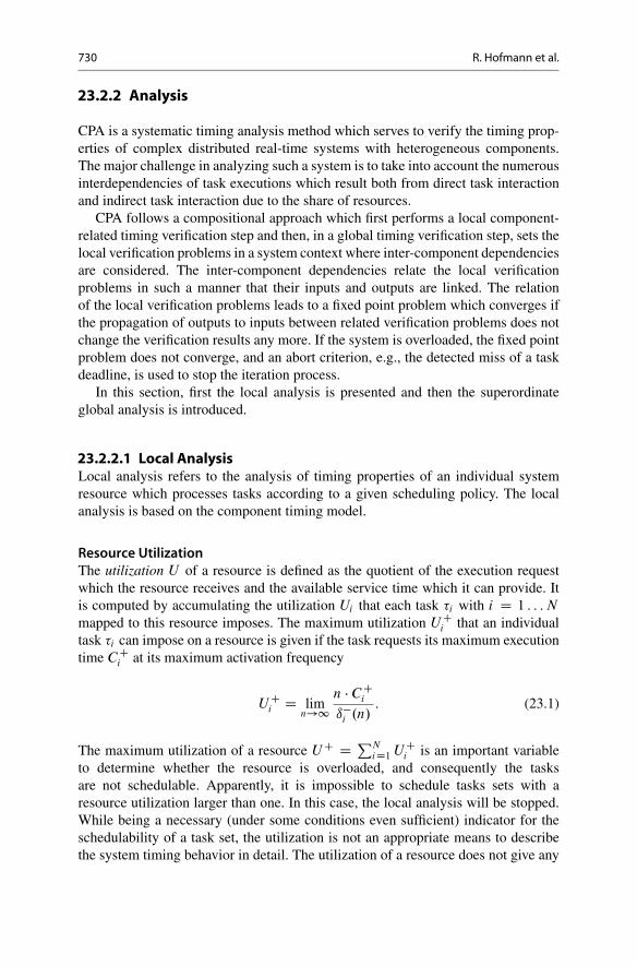
Worst-Case Response TimeSince tasks which are allocated to the same resource have to share its service, theprocessing of a task �i is preempted if other tasks with higher priority are activated.This is illustrated in Fig. 23.5. The time interval between the activation and thetermination of a task �i , including all suspension phases, is defined as the responsetime of task �i denoted as Ri . The minimum response time of task �i , denoted asR�

i , and the maximum response time of task �i , denoted as RCi , serve to bound the

response time behavior of task �i .The decisive property of hard real-time systems is that no task �i is allowed to

miss its deadline Di . In other words, it is required that the deadline Di is an upperbound on the worst-case response time RC

i . A major purpose of timing analysis likeCPA is to verify this system property which is crucial for safe operation of real-timesystems.

Determining the Worst-Case Response TimeIn order to verify whether the real-time requirement RC

i � Di for a task �i isfulfilled, the worst-case response time RC

i needs to be determined. Obviously, it isnot possible to explore the entire system state space for this purpose. Rather a worst-case scenario has to be derived which allows to find the worst-case response timeRC

i in a limited time window.The limited time window of system behavior comprising the worst-case response

time behavior of task �i is called the longest level-i busy period [23]. The longestlevel-i busy period is initiated by the so-called critical instant. The critical instantdescribes the alignment of task activations and the execution times which lead tothe maximum interference with respect to task �i and consequently to the worst-case response time RC

i . The longest level-i busy period closes if the investigation ofa longer time interval is known not to contribute any new information to the worst-case response time analysis. In the following, first the concept of the level-i busyperiod is explained. Then the multiple activation scheduling horizon as well as themultiple activation processing time processing time are introduced. Both of those

Fig. 23.5 Response time and relative deadline. Task �2 is preempted during execution by task�1 which is of higher priority. Therefore, the response time R2 is larger than the execution timeC2 D C2;1 C C2;2. The response time R2 is still smaller than the deadline D2


variables serve to formally describe the processing behavior of a local resource withrespect to task �i within the level-i busy period.

Busy PeriodA level-i busy period [23] is a time interval during which a resource R is busyprocessing a task �i or tasks of higher priority than task �i under a fixed priorityscheduling policy. Directly before and after the level-i busy period, the resource R

is idle with respect to task �i and tasks of higher priority.The level-i busy period is an elegant means to perform a worst-case response

time analysis by investigation of a limited time window. The idea is that the responsetime behavior of task �i in a level-i busy period is completely independent ofevents outside of this time interval. A level-i busy period is separated from thepreceding and succeeding level-i busy periods by idle phases of the resource R.An idle phase implies that the resource R is virtually reset to an initial state beingignorant of previous execution requests of task �i or tasks of higher priority. It isthus sufficient to investigate in the timing analysis the level-i busy period whichcomprises the worst-case response time behavior of task �i . This so-called longestlevel-i busy period is initiated by the critical instant, which creates the maximumpossible interference with respect to task �i so that the worst-case response time oftask �i can be observed within the longest level-i busy period. It is a skillful taskto derive this critical alignment of task activations and service requests for a givensystem configuration.

In the following, the longest level-i busy period and the initiating critical instantare derived for an SPP-scheduled task set on a single processing resource R with norestrictions on the task activation event models. Assume that at an instant t � �, theresource R is idle with respect to task �i and all tasks with higher priority. Shortlyafter at instant t , task �i is activated for the first time and requests its maximumexecution time C C

i . The activation causes the creation of the first task instance, alsocalled job, which is denoted as �i .1/. If all tasks with higher priority than task �i areactivated simultaneously with �i .1/ at t and request their maximum execution timeat the highest possible frequency, then the maximum interference with respect totask �i .1/ is evoked. This alignment of activations is the critical instant, the startingpoint of the longest level-i busy period. The level-i busy period generally comprisesmore than one job of task �i . The reason is that before job �i .1/ terminates, a secondactivation of task �i may occur. Consequently the resource stays busy processing job�i .2/ even if job �i .1/ terminated, and incoming jobs of tasks with priority higherthan task �i will preempt �i .2/ from time to time. The same may of course happenbefore job �i .2/ terminates etc., and only when a job of task �i finishes before a newactivation for task �i comes in and no tasks with higher priority are processed, thelevel-i busy period closes.

The critical instant for a task �i scheduled under an SPNP policy occurs (1) if task�i is activated simultaneously with all tasks of higher priority, (2) if task �i and alltasks of higher priority request their maximum execution times at highest possiblefrequency, and (3) if a task �j of lower priority, which has the largest execution time


among all tasks with a priority lower than task �i , started execution just previouslyto the first activation of task �i .

In the formal response time analysis, the closure of the level-i busy period isrepresented by the solution of a fixed point problem. In order to be able to formulatea formal response time analysis, the multiple activation scheduling horizon andthe multiple activation event processing time have to be introduced as done in thefollowing paragraphs. Both variables mathematically describe the timing behaviorof task �i within the level-i busy window.

Multiple Activation Scheduling HorizonThe q-activation scheduling horizon Si .q/ of task �i is defined as the maximumhalf-open time interval which starts with the arrival of the first job �i .1/ of anysequence of q consecutive jobs �i .1/; �i .2/; : : : �i .q/. The scheduling horizon closesat the (not included) point in time when a theoretical activation of task �i with aninfinitesimally short execution time � could be immediately served by the resourceR after the processing of the q consecutive jobs. This theoretical activation isindependent from the actual activation model of task �i since it is never actuallyexecuted [11].

The q-activation scheduling horizon generalizes the idea of the level-i busyperiod for a number q of activations. During the q-activation scheduling horizon,the resource R is busy processing task q jobs of �i and tasks of higher priority. Thecondition, which a theoretical activation with infinitesimally short execution time �

could be potentially served at the end of the scheduling horizon, enforces an idletime with respect to q jobs of task �i and all tasks of higher priority at the end of thescheduling horizon. The scheduling horizon for q D qC

i corresponds to the longestlevel-i busy period, where qC

i is the maximum number of activations of task �i

which fall into the scheduling horizon of their respective predecessor jobs

qCi D min fq � 1 j S.q/ < ı�

i .q C 1/g : (23.2)

For the SPP scheduling policy, the q-activation scheduling horizon Si .q/ is thesolution to the following fixed point equation

Si .q/ D q � C Ci C

Xj 2hp.i/

C Cj � �C

j .Si .q//: (23.3)

As can be seen in Eq. 23.3, the scheduling horizon Si .q/ is composed of two parts.Firstly, it contains the maximum time interval which is required to service q jobsof task �i . And secondly, it comprises the maximum interference caused by tasks ofhigher priority than task �i (hp.i/). The maximum interference is evoked if everytask �j with j 2 hp.i/ is activated according to its maximum arrival curve �C

j

and every job requests the worst-case execution time C Cj during Si .q/. At the end

of Si .q/, a hypothetical q C 1st activation of task �i with � execution time couldimmediately be served because all q jobs of task �i are processed and no jobs of


higher priority are pending. In case of the SPNP scheduling policy, the q-activationscheduling horizon Si .q/ has to take into account the worst-case one-time blockingcaused by a task of lower priority than task �i

Si .q/ D q � C Ci C max

j 2 lp.i/

nC C

j

oC

Xk 2 hp.i/

�Ck .Si .q// � C C

k : (23.4)

Therefore, Si .q/ is composed of (1) the maximum processing time of q jobs of task�i , (2) the maximum one-time blocking of task �i by a task of lower priority thantask �i due to non-preemption, and (3) the maximum interference of tasks with ahigher priority than task �i .

Multiple Activation Processing TimeThe q-activation processing time Bi .q/ is defined as the time interval starting withthe arrival of the first job �i .1/ and ending at the termination of job �i .q/ for anyq consecutive activations of task �i which fall into the scheduling horizon of theirrespective predecessors.

The maximum q-activation processing time BCi .q/ serves as basis for the worst-

case response computation. By definition, the maximum response time of the qthtask instance, denoted as RC

i .q/, is the difference of the maximum q-activationprocessing time of and its earliest possible time of activation

RCi .q/ D BC

i .q/ � ı�i .q/: (23.5)

The worst-case response time of a task �i , denoted as RCi , is the maximum response

time of task �i within the longest level-i busy period, respectively, the qCi -activation

scheduling horizon, thus

RCi D max

1�q�qCi

RCi .q/: (23.6)

For the SPP policy, the maximum q-activation processing time BCi .q/ is identical

to the q-activation scheduling horizon Si .q/ so that

BCi .q/ D q � C C

i CX

j 2hp.i/

C Cj � �C

j .BCi .q//: (23.7)

The identity of the q-activation processing time and the q-activation schedulinghorizon is due to the sub-additive behavior of the SPP scheduling policy with respectto the processing times [11, 39]: BC

i .q C p/ � BCi .q/ C BC

i .p/. This property is,however, not fulfilled for the SPNP scheduling policy. The maximum processingtime BC

i .q/ under the SPNP policy is the sum of the maximum queuing delay withrespect to job �i .q/, denoted as QC

i .q/, and the maximum execution time of job�i .q/


BCi .q/ D QC

i .q/ C C Ci : (23.8)

The maximum queuing delay QCi .q/ is the time a job �i .q/ has to wait before it

is selected for execution by the SPNP scheduler. Activations of tasks with a higherpriority than task �i which occur during the execution of the job �i .q/ do not prolongits processing time as by definition of the scheduling policy, it cannot be preemptedonce it has started executing. The queuing delay can be bounded from above by [10]

QCi .q/ D .q � 1/ � C C

i C maxj 2 lp.i/

nC C

j

oC

Xk 2 hp.i/

C Ck � �C

k .Qi .q/ C �/ :

(23.9)

The maximum queuing delay accounts for (1) the maximum execution demand ofall jobs of task �i activated prior to job �i .q/, (2) the longest one-time lower priorityblocking due to non-preemption, and (3) the longest higher priority blocking duringqueuing. The infinitesimally long time interval � added to the queuing delay servesto check whether another job interfering with task �i .q/ could start exactly at theend of the iteratively computed queuing delay, thus it extends the investigated timewindow. Note that Eq. 23.8–23.9 and Eq. 23.4 are not identical since the fixed pointiteration for BC

i .q/ accumulates higher priority interference only during the queuingdelay plus �, whereas Si .q/ takes also into account interference of higher priorityduring the execution of the qth job.

ExampleConsider the timing diagram in Fig. 23.6 which illustrates the concept of themultiple activation scheduling horizon and the multiple activation processing time.The timing diagram shows three tasks �1, �2, and �3 which are scheduled on acommon resource under an SPNP policy, where task �1 is of higher priority thantask �2 and task �2 is of higher priority than task �3. The scenario representsthe worst case with respect to the response time of task �2 since (1) task �3 isactivated just prior to tasks �1 and �2 with maximum execution demand, (2) task�1 causes maximum interference of higher priority, and (3) task �2 always requestsits maximum execution time at highest possible frequency.

In the timing diagram, the multiple activation scheduling horizons and themultiple activation processing times are indicated. All scheduling horizons andprocessing times start at time 0. The termination of job �2.1/ marks the end ofBC

2 .1/. The scheduling horizon S2.1/ is longer than BC2 .1/ due to the higher

priority interference which prevents that a hypothetical activation of task �2 with aninfinitesimally short execution time � could be immediately served after the first job�2.1/. Note that the scheduling horizon is defined as a half-open interval and thusdoes not take interference of higher priority into account which arrives exactly atthe interval boundary of S2.1/. Since the activation of �2.2/ falls into the schedulinghorizon S2.1/ of job �2.1/, BC

2 .2/ exists. Again, the scheduling horizon S2.2/ islonger than the processing time BC

2 .2/, but the activation of job �2.3/ does not fallinto the scheduling horizon S2.2/. Thus, S2.2/ is the longest scheduling horizon and


Fig. 23.6 Scheduling horizons and processing times for SPNP scheduling

represents the longest level-2 busy period. Note that the depicted scenario illustratesthe non-subadditive behavior of the processing times: BC

2 .2/ > BC2 .1/ C BC

2 .1/.The maximum processing time of job �2.1/ is BC

2 .1/ D 11, and its worst-caseresponse time equals RC

2 .1/ D BC2 .1/ � ı�.1/ D 11 � 0 D 11. The maximum

processing time of job �2.2/ is BC2 .1/ D 25, and its worst-case response time

equals RC2 .2/ D BC

2 .2/ � ı�.2/ D 25 � 15 D 10. Thus, a worst-case responsetime analysis yields the result RC

2 D max1�q�q

Ci

RC2 .q/ D 11.

Best-Case Response TimeThe best-case response time R�

i and the worst-case response time RCi serve to

bound the response time behavior of task �i . A simple approximation of the best-case response time R�

i relies on the following assumptions: (1) the absence ofinterference by tasks with equal or higher priority, and (2) the request of theminimum execution time C �

i .

R�i D C �

i : (23.10)

Even though this approximation does not necessarily represent a tight bound, it isusually acceptable as timing analysis aims to provide real-time guarantees and thusfocuses particularly on worst-case behavior.

JitterJitter represents the maximum time interval by which the occurrence of a given eventmay deviate from the expected occurrence of the event. The response time jitter ofa task �i can hence be calculated as the difference between the best-case responsetime RC

i and the worst-case response time R�i

Ji;resp D RCi � R�

i : (23.11)


BacklogIt is possible that an activation event for a task �i arrives before the previouslyactivated task instance has been processed, e.g., due to high interference or jitter. Inthis case, a backlog of activation events with respect to task �i arises. To prevent anyloss of information, all activation events are queued until they are processed. Thequeue semantics in CPA is characterized by a First-In First-Out (FIFO) organizationand a nondestructive write to and a destructive read from a queue storing activationevents. The determination of an appropriate queue size for pending activation eventsof task �i is important both to avoid dropping of events and over-dimensioning. Themaximum activation backlog for task �i , denoted as bC

i , is bounded by

bCi D max

1�q�qCi

˚0; �C

i .BCi .q/ C oi;out / � q C 1

�: (23.12)

The expression �C.�t/ represents the maximum possible number of task instanceswhich can be activated in �t , here with �t D BC

i .q/ C oi;out . The first termBC

i .q/ is the maximum processing time for the task instance q of �i , the secondterm oi;out represents the maximum overhead required to remove a finished taskinstance from the activation queue [13]. The term �q C 1 accounts for the factthat previously activated task instances have already been finished. In other words,Eq. 23.12 computes the difference between the number of occurred activation eventsand processed ones, hence returning the number of pending activation events.

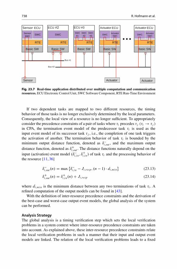
23.2.2.2 Global AnalysisIn the previous section on the principle of the local analysis, we have shown howto compute the worst-case and best-case response times, the output jitter and themaximum activation backlog for a task with a given activation model. The localanalysis is resource-related and does not consider any interaction between tasks ondifferent resources. However, in reality many real-time applications are composedof multiple tasks which are distributed over several resources. For instance, atypical real-time application performs a control function which evaluates andprocesses sensor data in order to control an actuator according to a given controllaw. An exemplary mapping of such a real-time application to a platform withcommunication and computation elements is illustrated in Fig. 23.7.

In this section, it is shown how the global analysis integrates the dependencies oftasks on different resources into the analysis.

Consideration of Global Precedence ConstraintsTasks in an application can generally not be executed in an arbitrary order buthave to be executed in a function-related order. The functional restrictions on thepossible execution orders of tasks are expressed in form of precedence constraints.Precedence constraints can be described by a directed graph, the nodes representingthe tasks, and the directed edges representing the directed execution dependencies.Paths in a precedence graph describe linear, branched, or even cyclic structures ofdependencies.


Fig. 23.7 Real-time application distributed over multiple computation and communicationresources. ECU Electronic Control Unit, SWC Software Component, RTE Run-Time Environment

If two dependent tasks are mapped to two different resources, the timingbehavior of those tasks is no longer exclusively determined by the local parameters.Consequently, the local view of a resource is no longer sufficient. To appropriatelyconsider the precedence constraints of a pair of tasks where �i precedes �j (�i ! �j )in CPA, the termination event model of the predecessor task �i is used as theinput event model of its successor task �j , i.e., the completion of one task triggersthe activation of another. The termination behavior of task �i is bounded by theminimum output distance function, denoted as ı�

i;out , and the maximum outputdistance function, denoted as ıC

i;out . The distance functions naturally depend on theinput (activation) event model .ı�

i;in; ıCi;in/ of task �i and the processing behavior of

the resource [11, 36]

ı�i;out .n/ D max

˚ı�

i;in � Ji;resp; .n � 1/ � di;min

�(23.13)

ıCi;out .n/ D ıC

i;in.n/ C Ji;resp (23.14)

where di;min is the minimum distance between any two terminations of task �i . Arefined computation of the output models can be found in [43].

With the definition of inter-resource precedence constraints and the derivation ofthe best-case and worst-case output event models, the global analysis of the systemcan be performed.

Analysis StrategyThe global analysis is a timing verification step which sets the local verificationproblems in a system context where inter-resource precedence constraints are takeninto account. As explained above, these inter-resource precedence constraints relatethe local verification problems in such a manner that their input and output eventmodels are linked. The relation of the local verification problems leads to a fixed


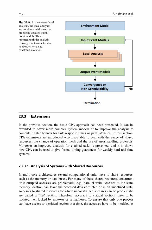
point problem which converges if the propagation of outputs to inputs betweenrelated verification problems does not change the verification results any more.Therefore, the CPA procedure consists of two parts: First, the local analysis ofthe individual resources is performed in order to generate the initial output eventmodels. Then in a global analysis step, the output event models are propagatedthrough the system to the tasks which utilize them as input event models due toglobal precedence constraints. The local analysis is repeated under updated inputparameters computing best-case and worst-case response times, jitter and requiredqueue sizes. Due to possible circular dependencies between activation models, itmight be necessary to repeat this process multiple times. This propagation of outputevent models and update of input event models is continued until the analysis resultsconverge.

In the following, the detailed procedure of the global analysis is presented whichis also illustrated in Fig. 23.8:

1. For every task �i which is activated by events in the system environment, theinput event model .ı�

i;in; ıCi;in/ is initialized with the input event model of the

respective external event source.2. For every task �j which is part of a precedence path, the input event model

.ı�j;in; ıC

j;in/ corresponds to the output event model of the predecessor task. If inthe initial analysis run no output event model of the predecessor task is available,then the input event model .ı�

j;in; ıCj;in/ is initialized with the input event model

of the predecessor task.3. A local analysis is performed for each resource with the objective of deriving the

task output event models. Additionally, it is checked if the local analysis resultsviolate any constraints, for instance, the required absence of system overload orthe guarantee of all task deadlines.

4. The computed task output event models are propagated through the system tothe tasks which utilize them as input event models due to respective precedenceconstraints.

5. If the propagated output event models are identical to the input event modelsused in the previous local analysis, a global fixed point has been reached andthe analysis terminates [46]. All timing constraints, particularly task deadlinesand end-to-end path latencies, are checked. The classical approach to computethe (worst case) end-to-end path latencies, is to accumulate the individual (worstcase) response times for each task along the path [21, 39, 47]. If any constraint isviolated, the system is not schedulable.

Otherwise, if no fixed point has been reached yet, the local analysis is repeatedwith the updated input event models.

If the CPA has successfully terminated, the Best-Case Response Times (BCRTs)and Worst-Case Response Times (WCRTs) of each task are known such that theresponse time behavior of every task can be safely bounded. Moreover, maximumrequired queue sizes are derived. Further system performance results can be derivedusing the supplementary analysis modules of CPA presented in Sect. 23.3.


Fig. 23.8 In the system-levelanalysis, the local analysesare combined with a step topropagate updated outputevent models. This isrepeated until the analysisconverges or terminates dueto abort criteria, e.g.,constraint violation

23.3 Extensions

In the previous section, the basic CPA approach has been presented. It can beextended to cover more complex system models or to improve the analysis tocompute tighter bounds for task response times or path latencies. In this section,CPA extensions are introduced which are able to deal with the usage of sharedresources, the change of operation modi and the use of error handling protocols.Moreover an improved analysis for chained tasks is presented, and it is shownhow CPA can be used to give formal timing guarantees for weakly-hard real-timesystems.

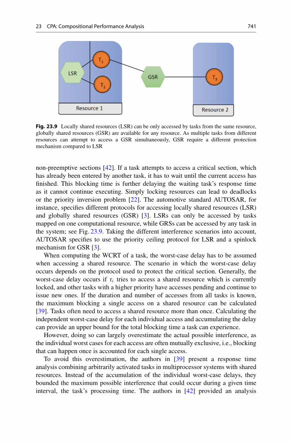
23.3.1 Analysis of Systems with Shared Resources

In multi-core architectures several computational units have to share resources,such as the memory or data buses. For many of these shared resources concurrentor interrupted accesses are problematic, e.g., parallel write accesses to the samememory location can leave the accessed data corrupted or in an undefined state.Accesses to shared resources for which unconstrained accesses can be problematicare called critical section. Therefore, accesses to critical sections have to beisolated, i.e., locked by mutexes or semaphores. To ensure that only one processcan have access to a critical section at a time, the accesses have to be modeled as


Fig. 23.9 Locally shared resources (LSR) can be only accessed by tasks from the same resource,globally shared resources (GSR) are available for any resource. As multiple tasks from differentresources can attempt to access a GSR simultaneously, GSR require a different protectionmechanism compared to LSR

non-preemptive sections [42]. If a task attempts to access a critical section, whichhas already been entered by another task, it has to wait until the current access hasfinished. This blocking time is further delaying the waiting task’s response timeas it cannot continue executing. Simply locking resources can lead to deadlocksor the priority inversion problem [22]. The automotive standard AUTOSAR, forinstance, specifies different protocols for accessing locally shared resources (LSR)and globally shared resources (GSR) [3]. LSRs can only be accessed by tasksmapped on one computational resource, while GRSs can be accessed by any task inthe system; see Fig. 23.9. Taking the different interference scenarios into account,AUTOSAR specifies to use the priority ceiling protocol for LSR and a spinlockmechanism for GSR [3].

When computing the WCRT of a task, the worst-case delay has to be assumedwhen accessing a shared resource. The scenario in which the worst-case delayoccurs depends on the protocol used to protect the critical section. Generally, theworst-case delay occurs if �i tries to access a shared resource which is currentlylocked, and other tasks with a higher priority have accesses pending and continue toissue new ones. If the duration and number of accesses from all tasks is known,the maximum blocking a single access on a shared resource can be calculated[39]. Tasks often need to access a shared resource more than once. Calculating theindependent worst-case delay for each individual access and accumulating the delaycan provide an upper bound for the total blocking time a task can experience.

However, doing so can largely overestimate the actual possible interference, asthe individual worst cases for each access are often mutually exclusive, i.e., blockingthat can happen once is accounted for each single access.

To avoid this overestimation, the authors in [39] present a response timeanalysis combining arbitrarily activated tasks in multiprocessor systems with sharedresources. Instead of the accumulation of the individual worst-case delays, theybounded the maximum possible interference that could occur during a given timeinterval, the task’s processing time. The authors in [42] provided an analysis


framework to calculate task timing behavior under the multi-core priority ceilingprotocol. In [28] the authors improved on this by taking into account localscheduling dependencies allowing to analyze sets of functional dependent tasks.The analysis has been extended to allow non-preemptive scheduling for tasks inmulti-core architectures with shared resources in [25].

23.3.2 Analysis of Systems Undergoing Mode Changes

Some real-time systems have to execute in multiple different modi, being able toadapt to the environment or the mission being executed in multiple stages. A plane,for instance, has to operate differently during start, landing, or flight, while in a carthe engine control might turn off certain analysis features, depending on the enginespeed [26]. With the capability to change its configuration, the system is able torun more efficiently as it only needs to execute tasks when necessary and disablesfunctions when no longer needed. Being able to deactivate unrequired functionscan prevent or reduce expensive hardware over-dimensionation. Switching betweendifferent configurations is called a mode change. This comes with the requirementto analyze and verify the safety not only under one static configuration, but of thedifferent operational modes and also of the transition phases. For real-time systems,this includes ensuring that the system satisfies all its deadlines during each possibleconfiguration.

A system is running in a steady state if it is executing in one mode without anyresiding influence from a previous mode change, only executing the tasks from thecorresponding task set. If the system receives a Mode Change Request (MCR) theset of running tasks has to be changed from the current mode to the new one. In orderto evaluate the transition phase, each task is classified according to the followingcategories:

1. Old tasks are tasks which were present in the previous mode but not in the newone. They are immediately terminated when the MCR occurs, i.e., any active orpending task instances are removed from the system.

2. Finished or completed tasks are tasks which were present in the previous modebut not in the new one. During the transition phase, these tasks are allowed tofinish their active and pending task instances, but no new instances will be started.

3. New or added tasks are tasks which are present in the new mode, but not in theold one. They can represent updated tasks from the old mode, e.g., with changedexecution time or activation pattern, or new functionalities.

4. Unchanged tasks are present during the old and new modes with identicalproperties, only in systems with periodicity.

If the system’s mode change protocol allows unchanged tasks, it is referred to aswith periodicity, and without periodicity if all task sets are disjunct.

When a MCR occurs, the system has to change from the current mode to the newone, remove old and finished tasks and add new tasks. If the system waits until all fin-ished tasks have completed their execution before starting to schedule new tasks, the


mode change protocol is called synchronous. Respectively, it is called asynchronous,if it starts scheduling new tasks right after the MCR has occurred, simultaneouslywith the last instances of finished tasks. Synchronous protocols ensure isolationbetween the modes and therefore do not require specific schedulability analysesfor the transition phase. However, due to the delay introduced by the separation ofthe modes, synchronous protocols are not always feasible, if the transition has tobe performed as fast as possible [27]. Asynchronous protocols, on the other hand,overcome this limitation and allow the simultaneous scheduling of tasks from theold and new mode. With an asynchronous protocol, the new tasks are added to theset of scheduled tasks, hence possibly increasing the resource utilization. As simplyadding new tasks to the current set can lead to temporal overload on the resource,asynchronous protocols require specific schedulability analyses [27, 34, 35, 50]. Forthe remainder of this section, we will focus be on asynchronous protocols.

The CPA approach provides functionality to analyze the WCRTs of tasks andpath latencies for a system in a certain mode. The transition periods can be modeledconservatively, by assuming that all tasks from the two (previous and new) modesare active simultaneously. In order to be able to model a transition phase, rules haveto be defined regarding which transition phases can occur. The CPA extension relieson the assumption that the system executes in a steady state when the MCR occurs,i.e., new mode changes are not allowed to arise, while an older MCR is still exertinginfluence on the task activations. With this restriction, only tasks from exactly twomode sets need to be considered for a transition phase. The outcome from this isthat not only the response times of tasks during steady states and the mode changephases are relevant but also the duration of these transition times. These transientlatencies determine the distance to the next possible mode change [27].

The authors in [27] have shown that due to complex task dependencies the effectsof a MCR are propagated delayed through the system, possibly causing feedback tothe source of the MCR. They have shown how to bound the transition latency, bydividing it into local task transition latencies and global system transition latencies.In [26] the authors evaluate options for the design of multi-core real-time systemsto minimize the impact of overly pessimistic measures taken in current practice.

23.3.3 Analysis of the Timing Impact of Errors and Error Handling

Safety-critical computing systems are usually designed to be fault tolerant towardcommunication and/or computation errors. However, each fault tolerance mecha-nisms incurs some time penalty because errors need first to be detected, and thenan error correction or error masking measure has to be taken. To guarantee thecorrect timing behavior of a fault-tolerant safety-critical computing system, a formalperformance analysis has to take these error-related, additional timing effects intoaccount.

The consideration of timing overhead of fault tolerance mechanisms requires theadaptation of the local CPA. The stochastic nature of errors involves the introductionof a stochastic busy period; this is described in Sect. 23.3.3.2. Apart from timing


overhead fault-tolerant systems have specific precedence constraints which result,for instance, from redundant task executions. In Sect. 23.3.3.1, an adapted worst-case response time analysis is briefly outlined for such fault-tolerant systems.

23.3.3.1 Computation Errors and Error HandlingA basic principle of detecting computational errors is to perform the same computa-tion several times and to compare the results. A discrepancy in the computed resultsis an evidence for an occurred fault. In a multi- or many-core processing system, it ispossible to parallelize the redundant computations or, respectively, the execution ofthe redundant tasks. Such a fault tolerance approach leads to fork-join task graphs,where forking means the parallel execution of replicated tasks and joining meanssynchronization and the comparison of results. In [5] a strategy is presented how toderive worst-case response times for tasks in a task set with fork-join precedenceconstraints, so that the timing impact of replicated and parallelized computationscan be evaluated.

23.3.3.2 Communication Errors and Error HandlingUnreliable communication links in data buses or packet-switched networks intro-duce bit errors in the digitally transmitted information. The occurrence of bit errorscan be modeled by stochastic processes which often use the average bit error rateor packet error rate as an important parameter. If the assumption of independent biterrors is justified, the Bernoulli process or its approximation as a Poisson process isa classical modeling choice. If the probability of a bit error depends on past events,a state-aware Markov process is more appropriate [44].

For multi-master data buses and point-to-point communication, the detection ofbit errors in transmitted frames at the receiver is typically based on error detectingcodes. If a an error has been detected and signaled, a retransmission of the thecorrupted or lost frame is initiated and the system is set back to a consistent state.Since bit errors can occur arbitrarily often albeit with a very low probability, thecomputation of a worst-case response time which includes an excessive detection,signaling, and correction time overhead is meaningless. A probabilistic schedulingguarantee, however, in the form of an exceedance function which specifies anupper bound on the probability that a task instance exceeds a reference responsetime value, is far more expressive. In [6], a probabilistic scheduling analysis ispresented for a fault-tolerant multi-master/point-to-point communication systemwith non-preemptive fixed priority arbitration which is, for instance, applicable toCAN. The analysis computes first the worst-case response time of a frame under1 : : : K errors and the corresponding probabilities, and then derives an exceedancefunction by summing up the probabilities for all error scenarios which have aworst-case response time smaller or equal than the reference response time. In [4],an improved approach is presented which relies on stochastic frame transmissiontimes. A stochastic frame transmission time is composed of the error-free frametransmission time and the stochastic overhead for error signaling and correction.


Stochastic frame transmission times give rise to stochastic busy periods from whichstochastic response times and a less pessimistic exceedance function can be derived.

The performance analysis of switched real-time networks, both on-chip and off-chip networks, is treated in [7]. The network switches are assumed to employ a fixedpriority-based arbitration scheme, and an end-to-end error protocol in form of anAutomatic Repeat Request (ARQ) scheme is investigated. In the ARQ scheme, thesender buffers a sent packet until an Acknowledgement (ACK) message is received.If no ACK arrives at the sender in a given time interval, a timeout occurs and thebuffered packet is retransmitted. The detection of corrupted packets at the receiveris typically based on error detecting codes. Both corrupted and lost packets aresignaled to the sender by an omitted acknowledgement so that a retransmissionis implicitly triggered. Variants of this type of ARQ error handling protocol areselective ARQ, stop-and-wait ARQ, and Go-back-N ARQ.

23.3.4 Refined Analysis of Task Chains

Real-time applications are usually not implemented as single tasks, but rather as aset of logical dependent tasks, as shown in Fig. 23.7. The tasks within an applicationare typically ordered and presented as a Directed Acyclic Graph (DAG), represent-ing the logical order of execution. Within such a graph any logical dependent tasksform a task path or task chain. Sensor-actuator chains in automotive or avionicsystems, for example, are distributed within the system as the components arephysically apart, or information needs to be gathered in a central instance to performdecision-making. Multimedia applications on the other hand are often pipelined inorder to process media streams more efficiently. To be able to take advantage of theparallelization of applications, the analyses methods need to support task paths andprovide mechanisms to efficiently analyze the dependencies between tasks.

The basic CPA approach supports the latency analysis of task paths, as describedin Sect. 23.2.2. The conservative approach is to compute the WCRT of each taskwhich is an element of the considered task path and to derive the path latencyby accumulating the individual WCRTs [21, 47]. While this simple accumulationprovides an upper bound for the path latency, it is pessimistic if local worst-casescenarios within the same path are mutually exclusive.

In [38] the authors consider the communication between application threadsand the corresponding precedence constraints in the resulting task graphs in orderto improve the local WCRTs. They exclude infeasible worst-case scenarios forlogically dependent tasks on the same SPP-scheduled resource by extending thescope of the busy period approach. By leveraging the particular semantics –including the distinction of synchronous and asynchronous communication – theywere able to significantly reduce pessimism and the analysis complexity, resultingin a faster execution of the local analysis.

Another situation, which can lead to especially large local WCRTs, occurs whena task is activated with a burst. Bursts can potentially occur anywhere within the


system, but the same burst cannot occur on all resources at once. Accumulating thelocal WCRTs from a path with a bursty activation event model can therefore leadto a significant overestimation. Pessimistically bounded WCRTs can translate intoover-dimensioning of the required hardware components and hence increased costs[39, 41]. This issue is captured in the ’pay burst only once’ problem [15].

In order to reduce the impact of the pay burst only once problem, the authorsin [40] proposed a method to identify relevant combinations of local responsetimes to derive a tighter worst-case path latency. They provided a methodologyfor computing path latencies, considering pipelined chains of tasks with transientoverload along the path. This approach was extended in [41] by enabling theanalysis of a wider variety of system topologies and including functional cyclesand nonfunctional dependencies.

A similar method can be used to improve the analysis of Ethernet networks.In Ethernet networks, different data streams often need to be transferred with thesame priority, as Ethernet switches only have a limited range of priorities. Streamswith the same priority are queued and transferred according to FIFO scheduling.Therefore, for the individual worst-case analyses, each other stream with the samepriority has be assumed to arrive simultaneously with the analyzed one but to beserved first [13].

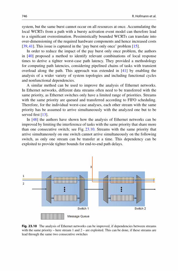
In [48] the authors have shown how the analysis of Ethernet networks can beimproved by limiting the interference of tasks with the same priority that share morethan one consecutive switch; see Fig. 23.10. Streams with the same priority thatarrive simultaneously on one switch cannot arrive simultaneously on the followingswitch, as only one stream can be transfer at a time. This dependency can beexploited to provide tighter bounds for end-to-end path delays.

Fig. 23.10 The analysis of Ethernet networks can be improved, if dependencies between streamswith the same priority – here stream 1 and 2 – are exploited. This can be done, if these streams arelead through the same two consecutive switches


23.3.5 Timing Verification of Weakly-Hard Real-Time Systems

Hard real-time computing systems require per definition that each instance of a taskmeets its deadline, whereas weakly-hard real-time systems tolerate occasional butin number and distribution precisely bounded deadline misses of tasks [8]. Forinstance, a weakly-hard system may require that a given task misses not morethan m deadlines in any sequence of k consecutive task activations. The tolerancetoward occasional deadline misses of tasks is usually based on the characteristicsof the implemented real-time applications. Prevalent real-time applications likecontrol functions, monitoring functions, and multimedia functions have shown tobe robust against occasional but bounded sample or frame losses which can beinterpreted as consequences of missed task deadlines. This robustness allows real-time applications to continue in safe operation even in the presence of limitedtransient overload [8, 16]. The analysis of weakly-hard real-time systems which isimplemented as an extension of CPA, called Typical Worst-Case Analysis (TWCA)[2,31,32,53], provides formal guarantees for the compliance with weakly-hard real-time requirements for a wide range of system configurations. It scales to real-sizedsystems and provides a good computational efficiency [30].

TWCA assumes that each task has a typical behavior, e.g., a periodic activationpattern, which is captured in a typical activation model. In rare circumstances, a taskmay additionally experience nontypical activations, e.g., sporadic activations [31] orsporadic bursts [32], and then can be described by its worst-case activation model.The distance between the typical and the worst-case activation model of a task iscaptured by the so-called overload model. In the typical worst case, which occurs ifall tasks show their densest pattern of typical activations and demand their maximumexecution time, no deadlines are missed. In the worst case, which occurs if all tasksshow their densest pattern of typical and nontypical activations and demand theirmaximum execution time, deadlines will be missed due to overload.

In two classical CPAs, the worst-case response times for both the typical worstcase and the worst-case behavior of the system are computed: Typical Worst-CaseResponse Time (TWCRT) and WCRT for all tasks. If the WCRT of a task �i exceedsits deadline, a deadline miss model is computed which indicates the maximumnumber of observable deadline misses m in any sequence of k of consecutiveinstances of task �i . The computation of the deadline miss model relies on threemain impact factors which need to be derived for each task interfering with task�i . Firstly, the overload model which is an indicator for how often nontypicalactivations can be encountered in a given time interval. Secondly, the longest timeinterval during which overload activations can impact the behavior of a sequence ofk of consecutive instances of task �i . And thirdly, the maximum number of deadlinemisses of task �i that can be traced back to one overload activation. The computeddeadline miss model for a task �i can be tightened if the number and distributionof overload activations, which induce the maximum number of deadline misses oftask �i in any sequence of k consecutive instances, are bounded as precisely aspossible [53].


23.3.6 Further Contributions

This chapter could only introduce the main functions of CPA. There are many morecontributions that exceed the available space and should only be mentioned.

The robustness of a system, for instance, determines how sensitive the systemreacts to changes in, e.g., execution and transmission delays, input data rates, orCPU clock cycles. A sensitivity analysis determines the influence of input data, orsystem configurations on the system robustness. The authors of [19, 20, 33] haveshown how to identify critical components for the system robustness and how tooptimize the platform. In many embedded systems, such as automotive systems,sensors are measuring the system behavior with a set period. If data is accessedperiodically, but the communication path, e.g., a FlexRay bus, is transmitting thedata with a different period, additional delay can occur due to the period mismatch.In [14] the authors discuss different end-to-end timing scenarios with a focus onregister-based communication, taking different aspects of end-to-end delays intoaccount.

23.4 Conclusion

In this chapter the compositional performance analysis approach has been presented.CPA provides a scalable framework to perform timing analysis of distributedembedded systems. It is widely used in the industrial development processes ofreal-time systems, especially in the automotive field where it is extensively provenin practice but also in avionics and even in networks-on-chip [12]. Numerousextensions exist to cover more complex applications, different applications of timinganalysis in sensitivity, and robustness as well as error analysis.

Acknowledgments The project leading to this overview has received funding from the EuropeanUnion’s Horizon 2020 research and innovation program under grant agreement No 644080 as wellas from the German Research Foundation (DFG) under the contract number TWCA ER168/30-1.

References

1. AbsInt. aiT. http://www.absint.com/ait/. Accessed 24 Feb 20162. Ahrendts L, Hammadeh ZAH, Ernst R (2016) Guarantees for runnable entities with heteroge-

neous real-time requirements (to appear). In: Design, automation & test in Europe conference& exhibition (DATE 2016)

3. Autosar (2011) Specification of operating system, 5.0.0 edn. http://autosar.org/download/R4.0/AUTOSAR_SWS_OS.pdf

4. Axer P, Ernst R (2013) Stochastic response-time guarantee for non-preemptive, fixed-priorityscheduling under errors. In: 50th ACM/EDAC/IEEE design automation conference (DAC2013), pp 1–7. doi:10.1145/2463209.2488946

5. Axer P, Quinton S, Neukirchner M, Ernst R, Dobel B, Hartig H (2013) Response-time analysisof parallel fork-join workloads with real-time constraints. In: 25th Euromicro conference onreal-time systems (ECRTS 2013), pp 215–224. doi:10.1109/ECRTS.2013.31

http://www.absint.com/ait/

http://autosar.org/download/R4.0/AUTOSAR_SWS_OS.pdf

http://autosar.org/download/R4.0/AUTOSAR_SWS_OS.pdf

http://dx.doi.org/10.1145/2463209.2488946

http://dx.doi.org/10.1109/ECRTS.2013.31


6. Axer P, Sebastian M, Ernst R (2012) Probabilistic response time bound for CAN messageswith arbitrary deadlines. In: Design, automation test in Europe conference exhibition (DATE2012), pp 1114–1117. doi:10.1109/DATE.2012.6176662

7. Axer P, Thiele D, Ernst R (2014) Formal timing analysis of automatic repeat request forswitched real-time networks. In: 9th IEEE international symposium on industrial embeddedsystems (SIES 2014), pp 78–87. doi:10.1109/SIES.2014.6871191

8. Bernat G, Burns A, Liamosi A (2001) Weakly hard real-time systems. IEEE Trans Comput50(4):308–321. doi:10.1109/12.919277

9. Bygde S (2010) Static WCET analysis based on abstract interpretation and counting ofelements. Mälardalen University, Västerås

10. Davis RI, Burns A, Bril RJ, Lukkien JJ (2007) Controller area network (CAN)schedulability analysis: refuted, revisited and revised. Real-Time Syst 35(3):239–272.doi:10.1007/s11241-007-9012-7

11. Diemer J (2016) Predictable architecture and performance analysis for general-purposenetworks-on-chip. Technische Universität Braunschweig, Braunschweig

12. Diemer J, Ernst R (2010) Back suction: service guarantees for latency-sensitive on-chipnetworks. In: Proceedings of the 2010 fourth ACM/IEEE international symposium onnetworks-on-chip (NOCS 2010). IEEE Computer Society, Washington, DC, pp 155–162.doi:10.1109/NOCS.2010.38

13. Diemer J, Rox J, Ernst R, Chen F, Kremer KT, Richter K (2012) Exploring the worst-case timing of ethernet AVB for industrial applications. In: Proceedings of the 38th annualconference of the IEEE industrial electronics society, Montreal. http://dx.doi.org/10.1109/IECON.2012.6389389

14. Feiertag N, Richter K, Nordlander J, Jonsson J (2008) A compositional framework for end-to-end path delay calculation of automotive systems under different path semantics. In:Proceedings of the IEEE real-time system symposium – workshop on compositional theoryand technology for real-time embedded systems, Barcelona, 30 Nov 2008

15. Fidler M (2003) Extending the network Calculus Pay bursts only once principle to aggregatescheduling. In: Proceedings of the quality of service in multiservice IP networks: secondinternational workshop, QoS-IP 2003 Milano, 24–26 Feb 2003. Springer, Berlin/Heidelberg,pp 19–34. doi:10.1007/3-540-36480-3-2

16. Frehse G, Hamann A, Quinton S, Wöhrle M (2014) Formal analysis of timing effects on closed-loop properties of control software. In: 35th IEEE real-time systems symposium 2014 (RTSS),Rome. https://hal.inria.fr/hal-01097622

17. GmbH S. SymTA/S and traceanalyzer. https://www.symtavision.com/products/symtas-traceanalyzer/. Accessed 29 Jan 2016

18. Gresser K (1993) An event model for deadline verification of hard real-time systems. In:Proceedings of the fifth Euromicro workshop on real-time systems, 1993, pp 118–123.doi:10.1109/EMWRT.1993.639067

19. Hamann A, Racu R, Ernst R (2006) A formal approach to robustness maximization of complexheterogeneous embedded systems. In: Proceedings of the international conference on hardware– software codesign and system synthesis (CODES), Seoul

20. Hamann A, Racu R, Ernst R (2007) Multidimensional robustness optimization in heteroge-neous distributed embedded systems. In: Proceedings of the 13th IEEE real-time and embeddedtechnology and applications symposium

21. Henia R, Hamann A, Jersak M, Racu R, Richter K, Ernst R (2005) System level perfor-mance analysis – the symTA/S approach. IEE Proc Comput Digit Tech 152(2):148–166.doi:10.1049/ip-cdt:20045088

22. Lampson BW, Redell DD (1980) Experience with processes and monitors in mesa. CommunACM 23(2):105–117. doi:10.1145/358818.358824

23. Lehoczky JP (1990) Fixed priority scheduling of periodic task sets with arbitrarydeadlines. In: Proceedings of the 11th real-time systems symposium, pp 201–209.doi:10.1109/REAL.1990.128748

24. Liu JW (2000) Real-time systems. Prentice Hall, Englewood Cliffs

http://dx.doi.org/10.1109/DATE.2012.6176662

http://dx.doi.org/10.1109/SIES.2014.6871191

http://dx.doi.org/10.1109/12.919277

http://dx.doi.org/10.1007/s11241-007-9012-7

http://dx.doi.org/10.1109/NOCS.2010.38

http://dx.doi.org/10.1109/IECON.2012.6389389

http://dx.doi.org/10.1109/IECON.2012.6389389

http://dx.doi.org/10.1007/3-540-36480-3-2

https://hal.inria.fr/hal-01097622

https://www.symtavision.com/products/symtas-traceanalyzer/

https://www.symtavision.com/products/symtas-traceanalyzer/

http://dx.doi.org/10.1109/EMWRT.1993.639067

http://dx.doi.org/10.1049/ip-cdt:20045088

http://dx.doi.org/10.1145/358818.358824

http://dx.doi.org/10.1109/REAL.1990.128748


25. Negrean M, Ernst R (2012) Response-time analysis for non-preemptive scheduling in multi-core systems with shared resources. In: Proceedings of the 7th IEEE international symposiumon industrial embedded systems (SIES), Karlsruhe

26. Negrean M, Ernst R, Schliecker S (2012) Mastering timing challenges for the design of multi-mode applications on multi-core real-time embedded systems. In: 6th international congresson embedded real-time software and systems (ERTS), Toulouse

27. Negrean M, Neukirchner M, Stein S, Schliecker S, Ernst R (2011) Bounding mode changetransition latencies for multi-mode real-time distributed applications. In: 16th IEEE interna-tional conference on emerging technologies and factory automation (ETFA 2011), Toulouse.http://dx.doi.org/10.1109/ETFA.2011.6059009

28. Negrean M, Schliecker S, Ernst R (2009) Response-time analysis of arbitrarily activated tasksin multiprocessor systems with shared resources. In: Proceedings of the Design, Automa-tion, and Test in Europe (DATE), Nice. http://ieeexplore.ieee.org/xpls/abs_all.jsp?arnumber=5090720

29. Pellizzoni R, Schranzhofer A, Chen JJ, Caccamo M, Thiele L (2010) Worst case delayanalysis for memory interference in multicore systems. In: Design, automation test in Europeconference exhibition (DATE 2010), pp 741–746. doi:10.1109/DATE.2010.5456952

30. Quinton S, Ernst R, Bertrand D, Yomsi PM (2012) Challenges and new trends in probabilistictiming analysis. In: Design, automation & test in Europe conference & exhibition (DATE2012), pp 810–815. doi:10.1109/DATE.2012.6176605

31. Quinton S, Hanke M, Ernst R (2012) Formal analysis of sporadic overload in real-timesystems. In: Design, automation test in Europe conference exhibition (DATE), pp 515–520.doi:10.1109/DATE.2012.6176523

32. Quinton S, Negrean M, Ernst R (2013) Formal analysis of sporadic bursts in real-timesystems. In: Design, automation test in Europe conference exhibition (DATE), pp 767–772.doi:10.7873/DATE.2013.163

33. Racu R, Hamann A, Ernst R (2008) Sensitivity analysis of complex embedded real-timesystems. Real-Time Syst 39:31–72

34. Rafik Henia RE (2007) Scenario aware analysis for complex event models and distributedsystems. In: Proceedings real-time systems symposium

35. Real J, Crespo A (2004) Mode change protocols for real-time systems: a survey and a newproposal. Real-Time Syst 26(2):161–197. doi:10.1023/B:TIME.0000016129.97430.c6

36. Richter K (2005) Compositional scheduling analysis using standard event models. Ph.D. thesis,TU Braunschweig, IDA

37. Richter K, Jersak M, Ernst R (2003) A formal approach to MpSoC performance verification.Computer 36(4):60–67

38. Schlatow J, Ernst R (2016) Response-time analysis for task chains in communicating threads.In: 22nd IEEE real-time embedded technology and applications symposium (RTAS 2016),Vienna

39. Schliecker S (2011) Performance analysis of multiprocessor real-time systems with sharedresources. Ph.D. thesis, Technische Universität Braunschweig, Braunschweig. http://www.cuvillier.de/flycms/de/html/30/-UickI3zKPS76fkY=/Buchdetails.html

40. Schliecker S, Ernst R (2008) Compositional path latency computation with local busy times.Technical report IDA-08-01, Technical University Braunschweig, Braunschweig

41. Schliecker S, Ernst R (2009) A recursive approach to end-to-end path latency computation inheterogeneous multiprocessor systems. In: Proceedings of the 7th international conference onhardware software codesign and system synthesis (CODES-ISSS). ACM, Grenoble. http://doi.acm.org/10.1145/1629435.1629494

42. Schliecker S, Negrean M, Ernst R (2009) Response time analysis in multicore ECUs withshared resources. IEEE Trans Ind Inf 5(4):402–413. http://ieee-ies.org/tii/issues/iit09_4.shtml

43. Schliecker S, Rox J, Ivers M, Ernst R (2008) Providing accurate event models for theanalysis of heterogeneous multiprocessor systems. In: Proceedings of the 6th IEEE/ACM/IFIPinternational conference on Hardware/Software codesign and system synthesis. ACM, pp 185–190

http://dx.doi.org/10.1109/ETFA.2011.6059009

http://ieeexplore.ieee.org/xpls/abs_all.jsp?arnumber=5090720

http://ieeexplore.ieee.org/xpls/abs_all.jsp?arnumber=5090720





http://dx.doi.org/10.1023/B:TIME.0000016129.97430.c6

http://www.cuvillier.de/flycms/de/html/30/-UickI3zKPS76fkY=/Buchdetails.html

http://www.cuvillier.de/flycms/de/html/30/-UickI3zKPS76fkY=/Buchdetails.html

http://doi.acm.org/10.1145/1629435.1629494

http://doi.acm.org/10.1145/1629435.1629494

http://ieee-ies.org/tii/issues/iit09_4.shtml


44. Sebastian M, Axer P, Ernst R (2011) Utilizing hidden Markov models for formal re-liability analysis of real-time communication systems with errors. In: IEEE 17th Pa-cific Rim international symposium on dependable computing (PRDC 2011), pp 79–88.doi:10.1109/PRDC.2011.19

45. Service ASC. Arinc 600 series. http://store.aviation-ia.com/cf/store/catalog.cfm?prod_group_id=1&category_group_id=3. Accessed 16 Mar 2016

46. Stein S, Diemer J, Ivers M, Schliecker S, Ernst R (2008) On the convergence of the symta/sanalysis. Technical report, TU Braunschweig, Braunschweig

47. Sun J, Liu JWS (1995) Bounding the end-to-end response time in multiprocessor real-timesystems. In: Proceedings of the third workshop on parallel and distributed real-time systems,1995, pp 91–98. doi:10.1109/WPDRTS.1995.470502

48. Thiele D, Axer P, Ernst R (2015) Improving formal timing analysis of switched ethernet byexploiting fifo scheduling. In: Design automation conference (DAC), San Francisco

49. Thiele L, Chakraborty S, Naedele M (2000) Real-time calculus for scheduling hard real-timesystems. In: Proceedings of the IEEE international symposium on circuits and systems. Emerg-ing technologies for the 21st century, 2000, pp 101–104. doi:10.1109/ISCAS.2000.858698

50. Tindell KW, Burns A, Wellings AJ (1992) Mode changes in priority preemp-tively scheduled systems. In: Real-time systems symposium, 1992, pp 100–109.doi:10.1109/REAL.1992.242672

51. Wilhelm R, Engblom J, Ermedahl A, Holsti N, Thesing S, Whalley D, Bernat G, Ferdinand C,Heckmann R, Mitra T, Mueller F, Puaut I, Puschner P, Staschulat J, Stenstrom P (2008) Theworst-case execution time problem – overview of methods and survey of tools. ACM TransEmbed Comput Syst 7(3):Art. 36

52. Wilhelm R, Engblom J, Ermedahl A, Holsti N, Thesing S, Whalley D, Bernat G, Ferdinand C,Heckmann R, Mitra T, Mueller F, Puaut I, Puschner P, Staschulat J, Stenström, P (2008) Theworst-case execution-time problem—overview of methods and survey of tools. ACMTrans Embed Comput Syst 7(3):36:1–36:53. doi:10.1145/1347375.1347389

53. Xu W, Hammadeh Z, Quinton S, Kröller A, Ernst R (2015) Improved deadline miss modelsfor real-time systems using typical worst-case analysis. In: 27th Euromicro conference on real-time systems (ECRTS), Lund

http://dx.doi.org/10.1109/PRDC.2011.19

http://store.aviation-ia.com/cf/store/catalog.cfm?prod_group_id=1&category_group_id=3

http://store.aviation-ia.com/cf/store/catalog.cfm?prod_group_id=1&category_group_id=3

http://dx.doi.org/10.1109/WPDRTS.1995.470502

http://dx.doi.org/10.1109/ISCAS.2000.858698

http://dx.doi.org/10.1109/REAL.1992.242672

http://dx.doi.org/10.1145/1347375.1347389

Documents

Robin Hofmann, Leonie Ahrendts, and Rolf Ernst