AD-A238 : Q54lIllI lIII III 1111 111 11111 11111 l ii lliiil

ARI Research Note 91-83 I.

The Effects of Selective ReenlistmentBonuses, Part I: Background and

Theoretical Issues

Robert TinneyU.S. Army Research Institute

Manpower and Personnel Policy Research GroupMichael E. Benedict, Acting Chief

Manpower and Personnel Research LaboratoryZita M. Simutis, Director

June 1991

91-06071

United States ArmyResearch Institute for the Behavioral and Social Sciences

Approved for public release; distribution is unlimited.

910

U.S. ARMY RESEARCH INSTITUTEFOR THE BEHAVIORAL AND SOCIAL SCIENCES

A Field Operating Agency Under the Jurisdictionof the Deputy Chief of Staff for Personnel

EDGAR M. JOHNSON JON W. BLADESTechnical Director COL, IN

Commanding

Technical review by

Cyril E. Kearl

NOTICES

DISTRIBUTION: This report has been cleared for release to the Defense Technical InformationCenter (DTIC) to comply with regulatory requirements. It has been given no primary distributionother than to DTIC and will be available only through DTIC or the National TechnicalInformation Service (NTIS).

FINAL DISPOSITION: This report may be destroyed when it is no longer needed. Please do notreturn it to the U.S. Army Research Institute for the Behavioral and Social Sciences.

NOTE: The views, opinions, and findings in this report are those of the author(s) ard should notbe construed as an official Department of the Army position, policy, or decision, unless sodesignated by other authorized documents.

THE EFFECTS OF SELECTIVE REENLISTMENT BONUSES, PART I:BACKGROUND AND THEORETICAL ISSUES

CONTENTS

Page

INTRODUCTION...........................1

Historical Development of Reenlistment BonusPrograms......................................................1Cost-Effectiveness of the SRB Program............3

METHODOLOGICAL ISSUES IN REENLISTMENT RESEARCH ......... 6

Research Through the Mid-1970s..................6Key Questions and Models foz ReenlistmentResearch..............................8

THE ECONOMIC THEORY OF OCCUPATIONAL CHOICE.............13

ACOL MODEL RESEARCH.......................18

The Acol M odel..........................18

Review of Acol Literature and Related Research.........20

THE SECOND GENERATION ACOL (ACOL-2) MODEL............24

IMPLICATIONS..........................27

REFERENCES...............................29

UNCLASSIFIEDSECURITY CLASSIFICATION OF THIS PAGE

Form ApprovedREPORT DOCUMENTATION PAGE OMNo. 0704-0188

la. REPORT SECURITY CLASSIFICATION lb. RESTRICTIVE MARKINGS

Unclassified --

2a. SECURITY CLASSIFICATION AUTHORITY 3. DISTRIBUTION /AVAILABILITY OF REPORT-- __Approved for public release;2b. DECLASSIFICATION /DOWNGRADING SCHEDULE distribution is unlimited.

4. PERFORMING ORGANIZATION REPORT NUMBER(S) 5. MONITORING ORGANIZATION REPORT NUMBER(S)

ARI Research Note 91-83 --

6a. NAME OF PERFORMING ORGANIZATION 6b. OFFICE SYMBOL 7a. NAME OF MONITORING ORGANIZATION(If applicable)

U.S. Army Research Institute PERI-RG

6c. ADDRESS (City, State, and ZIP Code) 7b. ADDRESS (City, State, and ZIP Code)

5001 Eisenhower AvenueAlexd.iiLia, VA 22333-5600

8a. NAME OF FUNDING/SPONSORING 8b. OFFICE SYMBOL 9. PROCUREMENT INSTRUMENT IDENTIFICATION NUMBERORGANIZATION U.S. Army Research (If applicable)

Institute for the Behavioraland Social Sciences PERI-R --

8c. ADDRESS (City, State, and ZIP Code) 10. SOURCE OF FUNDING NUMBERS

Alexandria, VA 22333-5600 ELEMENT NO. NO. NO. ACCESSION NO.

AA63007A 792 2301 H04

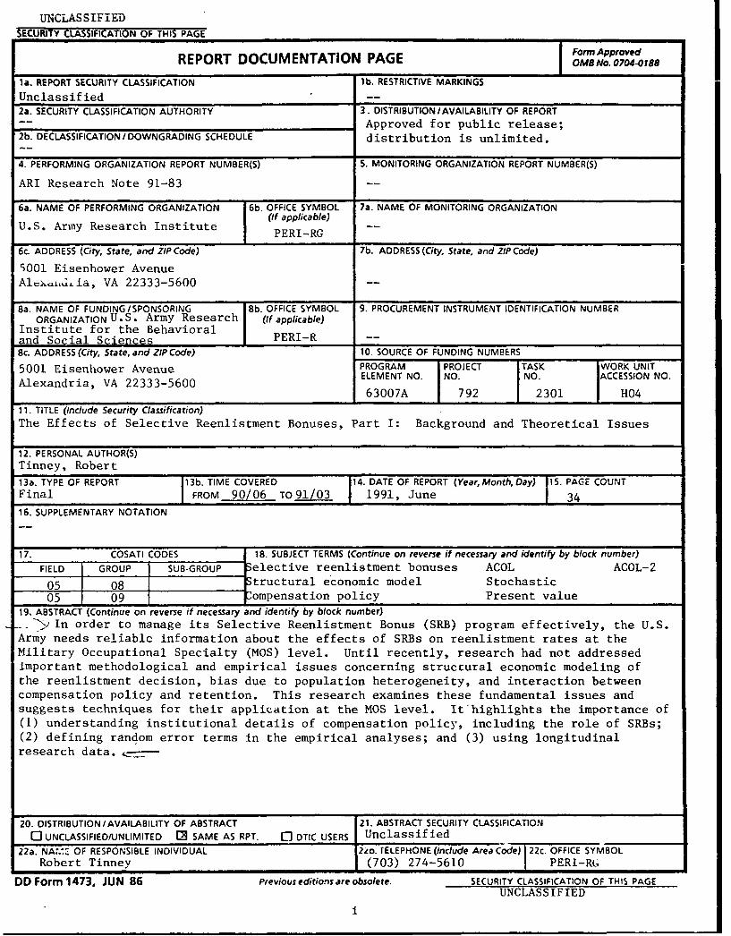
11. TITLE (Include Security Classification)The Effects of Selective Reenlistment Bonuses, Part I: Background and Theoretical Issues

12. PERSONAL AUTHOR(S)Tinney, Robert

13a. TYPE OF REPORT 13b. TIME COVERED 114. DATE OF REPORT (Year, Month, Day) 15. PAGE COUNTFinal I FROM 90/06 TO91/03 1991, June 34

16. SUPPLEMENTARY NOTATION

17. COSATI CODES 18. SUBJECT TERMS (Continue on reverse if necessary and identify by block number)

FIELD GROUP SUB-GROUP elective reenlistment bonuses ACOL ACOL-2

05 08 tructural economic model Stochastic

05 09 Fompensation policy Present value

19, ABSTRACT (Continue on reverse if necessary and identify by block number)---- > In order to manage its Selective Reenlistment Bonus (SRB) program effectively, the U.S.Army needs reliablc information about the effects of SRBs on reenlistment rates at theMilitary Occupational Specialty (MOS) level. Until recently, research had not addressedimportant methodological and empirical issues concerning structural economic modeling of

the reenlistment decision, bias due to population heterogeneity, and interaction betweencompensation policy and retention. This research examines these fundamental issues andsuggests techniques for their application at the MOS level. It highlights the importance of(1) understanding institutional details of compensation policy, including the role of SRBs;(2) defining random error terms in the empirical analyses; and (3) using longitudinal

research data. ,-

20. DISTRIBUTION/AVAILABILITY OF ABSTRACT 21. ABSTRACT SECURITY CLASSIFICATION

0 UNCLASSIFIED/UNLIMITED [ SAME AS RPT. C] DTIC USERS Unclassified

22a. NA%'.:' OF RESPONSIBLE INDIVIDUAL io. TELEPHONE (Include Area Code) 22c. OFFICE SYMBOL

Robert Tinney (703) 274-5610 PERI-RG

DD Form 1473. JUN 86 Previous editions are obsolete. SECURITY CLASSIFICATION OF THIS PAGEUNCLASSIFIED

THE EFFECTS OF SELECTIVE REENLISTMENT BONUSES, PART I:BACKGROUND AND THEORETICAL ISSUES

INTRODUCTION

Historical Development of Reenlistment Bonus Programs

The purpose of Selective Reenlistment Bonuses (SRBs) is to"provide a monetary incentive to encourage enlisted uniformedservices personnel in critical skill specialties with hightraining costs to reenlist."' Reenlistment bonuses for the Armywere first authorized by the Act of March 3, 1791, whichestablished a lump sum bonus of $6 for a reenlistment. Ofcourse, there have been many changes in reenlistment bonusprograms since that time. One characteristic has remainedunaltered, however. In order to qualify for the bonus, enlistedpersonnel must serve "continuously" by reenlisting "immediately."

Among the changes that have occurred are the uniformedservices covered, eligibility requirements, methods of payment(e.g. lump sum vs. installment), and length of serviceobligation. Reenlistment bonuses were first authorized forMarines in 1854 and Navy personnel in 1855. Lump sum bonuseswere also replaced by annual installment payments in 1854. In aneffort to establish a consistent approach to reenlistmentbonuses, Congress passed the Joint Services Pay Act of 1922.This law mandated a service-wide reenlistment bonus of $50 by thenumber of years served in the term of service from which themember was last discharged. Additional pay could be receivedbased on total rather than continuous length of service. Ineffect, the financial incentive to reenlist recognized the valueof experience.

The Career Compensation Act of 1949 substantially alteredreenlistment bonus programs. First, the Act required that yearsof future obligated service, rather than past service, be used tocompute bonus amounts. Second, bonuses increased with length ofobligated service to encourage longer reenlistments. Third,career limits were placed on (1) the number of times and lengthof obligated service during which bonuses could be received and(2) the cumulative amount of bonuses. Congress modified bonusesfurther by authorizing regular reenlistment bonuses (RRB) in theAct of July 16, 1954. This program directed relatively more ofthe budget for reenlistment bonuses to first term reenlistments,reduced the career total obligated service during which bonusescould be received (from 30 to 20), and increased the careerdollar limit.

1 The historical context of reenlistment bonuses and the

development of the SRB program are described in the third editionof Military Compensation Background Papers, Department OfDefense(1987).

1

The services subsequently experienced shortages of firstterm personnel in technical, high training-cost skills. Thevariable reenlistment bonus (VRB) program was authorized by theAct of August 23, 1965 to address these shortages. Under the VRBprogram, bonuses were computed as multiples of RRBs. The maximumVRB payment was not to exceed four times the RRB amount. Thislimited VRBs to a maximum of $bOOO because the maximum RRB was$2000. Four VRB multiplier levels were determined on the basisof first term training costs and shortages in critical skills.

RRBs were paid to all members of the military whether or notthey were in critical shortage skill categories. Consequently,bonuses were paid to personnel in skill categories that did nothave retention problems and could have been maintained atadequate levels without them. The Department of Defense (DCrh'.estimated that $43 million was spent unnecessarily for thisreason in fiscal years 1972 and 1973. During this period, aproblem with the VRB program also became apparent. VRBs couldonly be paid for first term reenlistments and could not be usedto address retention problems in critical skills at the secondand third term reenlistments. The Selective Reenlistment Bonusprogram was authorized by the Armed Forces Personnel Bc. usRevision Act of 1974 to correct these problems.

Initially, the Act provided payment of SRBs not to exceed$15000 to members who: (1) had completed at least 21 months butnot more than ten years of active service, (2) had a skilldesignated as critical, and (3) reenlisted or extended anexisting enlistment for at least three years. Obligated servicebeyond twelve years could not be used in computing SRB payments.The Department of Defense Authorization Act of 1981 expandedcoverage of the original SRB authorization to include memberswith up to fourteen years of active service. With this change,obligated service that could be used in computing SRB paymentswas limited to sixteen years. This regulation is still ineffect. The maximum bonus amount was also increased to $20000for members with nuclear skills and $16000 for everyone else.The maximum was further increased to $30000 in 1987.

The method of payment of SRBs has also undergone majorchanges since they were first authorized. Initially, bonuseswere paid in equal annual installments over the period ofobligated service. In 1979, Congress added a lump sum optionwhich allowed payment of the entire amount of bonus at thebeginning of a new reenlistment or extension of an existingenlistment. In 1982, this was changed so that fifty percent ofthe bonus could be paid as a lump sum and the remainder in equalannual installments. Members could still elect to be paid inequal annual installments. The DOD Authorization Act of 1986changed the percentage for lump sum amounts from fifty to atleast seventy five percent. However, this change has yet to beimplemented.

2

Other important aspects of the SRB program are regulationsdeveloped by the Secretary of Defense to implement SRBauthorization. Three eligibility zones have been establishedcorresponding to first, second, and third term reenlistments.Zone A is for reenlistments between 21 months and six years ofservice, Zone B reenlistments are between six and ten years, andZone C reenlistments are between ten and fourteen years. Amember completing between 21 months continuous and six yearstotal active duty can qualify for a Zone A SRB. A member whocompletes between six and ten years of continuous active duty canqualify for a Zone B SRB whether or not he/she received a Zone ASRB. Similarly, members completing between ten and fourteenyears of continuous active duty can qualify for a Zone C SRB,regardless of whether a Zone A or Zone B SRB was received.

Members are limited to one SRB in each zone, must possess a"critical" skill, be in pay grade E-3 or higher, and reenlist orextend an enlistment at least three years to qualify for an SRBin any zone. In addition, a reenlistment or extension whencombined with a member's completed active service time must totalat least six years of service for Zone A, ten years for Zone B,and fourteen years for Zone C. Those nembers eligible toreenlist may do so (or extend an existing enlistment) up to eightmonths prior to his/her expiration-of-term of service (ETS)date.2 Finally, six levels of skill "criticality" have beenauthorized for the military services for computation of SRBpayments.

The computation of SRBs is straight forward. A member'sbonus is the product of the skill criticality factor, ormultiplier, designated for his/her military occupationalspeciality, (MOS) monthly basic pay, and number of years ofactive obligated service (not to extend beyond sixteen years).For example, the SRB Pultiplier for the Army's Imagery AnalystMOS 96D was 5.0 in FY 1985. That year, the basic pay of soldiersin pay grade E-4 with three years of service was $10,292, or$858 per month. The SRB payment to soldiers in this pay gradewho reenlisted for three more years in 96D would therefore havebeen $12,865 (= 3x5.0x$858/mo.).

Cost-Effectiveness of the SRB Program

With the change from the draft to the All Volunteer Force(AVF) in 1973, the focus of military personnel policy shifted tomeeting career military manpower requirements through theretention of highly trained qualified personnel. In thissetting, SRBs became an important element in a system offinancial and non-financial incentives designed to make activemilitary service an attractive alternative to civilianoccupations. Since 1974, SRB program expenditures for all

2 Regulations governing reenlistment in the Army are in

Army Regulation 635-200, Department of the Army (1988).

3

uniformed services increased from $126 million in 1974 to a highof $487 million in 1985, an increase of almost four fold.3 Inproportional terms, SRB expenditures increased from .1 percent oftotal military compensation to 2.3 percent during this period.

SRB expenditures by the Army followed a similar pattern.Actual SRB payments rose from $44.5 to $140.5 million betweenfiscal years 1975 and 1986, and then declined to $88.4 million infiscal 1991.4 These fluctuations reflect changes in the size ofthe enlisted force and compensation policy. SRB payments by alluniformed services doubled in the 1980's compared to the 1970s asthe number of enlisted personnel increased and military pay rose.Similarly, the Army's SRB expcnditures reached a high of $145million in 1981 and, with one exception, remained above $100million until fiscal year 1989, when the Army began to downsizethe enlisted force.

SRB payments are a small proportion of the Army's personnelcosts (as well as the other uniformed services) because they area supplement to basic pay and are selective. They may beallocated to prevent manpower shortages in occupations criticalto the readiness capability of the force. For the SRB program toaccomplish this mission effectively and efficiently, informationis needed about (1) critically important MOS (2) retention ratesand "desired" force levels in critically important MOS, (3) theeffects of bonus payments on retention in these MOS and (4) thecosts of the SRB program. Understanding the relationship betweenbonus payments and SRB multipliers is also important because theArmy determines bonuses by selecting SRB multiplier levels.

Historically, the Army has used a subjective process toselect MOS that qualify for SRBs and define multiplier levels forthose MOS.5 Factors considered in this process includeauthorization levels for MOS, retention rates, per cent "fill" inMOS (i.e., difference between retention rate and authorization),training costs, pay grade, and SRB zones. These factors along

3 Dept. of Defense (1987).

4 The SRB expenditure data for the Army were obtained fromthe Force Alignment Division of the U.S. Personnel Command(PERSCOM), now Total Army Personnel Command.

5 The discussion in the text is an overview of a complexprocess used to manage the SRB program by personnel in the ForceAlignment Division of PERSCOM and the Office of the Deputy Chiefof Staff for Personnel (ODSCPER), U.S. Army. This is summarizedin "Selective Reenlistment Bonus Decision Support System(SRB.DSS) Study Directive", ODCSPER, 28 Aug 86, p. 3. See alsoAction Memorandum "Development of a Selective Reenlistment Bonus(SRB) Database and SRB Modules Within the Headquarters,Department of the Army.

4

with others are used as criteria in the selection of multiplierlevels.

Estimates of the effects of multipliers on reenlistmentrates for ten broad skill groupings are used to estimate thecosts of the SRB program and provide a check of the cost-effectiveness of multipliers selected for the SRB program. Theseestimates are not however applied in the current process ofsetting SRB multipliers and are inadequate for this purpose.First, they are results of a research completed in 1983 andtherefore based on data that are out of date. Secondly, theestimates attempt to measure the effects of multipliers rathelthan bonus payments themselves. In addition, they include theeffects of other factors correlated with bonus multipliers thathave an impact on reenlistments. These factors includeunobserved differences in preference for Army life, other formsof compensation, and the interaction between compensation policyand retention. Finally, the skill groupings are not MOS specificand do not correspond to the current Career Management Field(CMF) definition of skill categories.

In this context, the U.S. Army Research Institute (ARI)undertook economic research to evaluate the effects of SRBpayments on retention at the MOS level. The informationobjectives of the research are spelled out by the Office of theDeputy Chief of Staff for Personnel (ODCSPER), U.S. Army asfollows :6

"Further, it is impossible to subjectively determine theappropriate multiplier level for a MOS in a cost-effectivemanner without modeling the expected reenlistment responseto the SRB by the soldiers in the MOS. A methodology isneeded to improve the selection of multiplier levels so thatthe Army may better meet the needs of MOS given aconstrained budget environment." (1986, p.3).

Economic theory and military manpower research are reviewedin this report to identify relevant methodological issues andalternative techniques. Results of early research are summarizedin the section on methodological issues. The focus of thediscussion is on fundamental research issues that need to beaddressed in reenlistment research. A structural economic modelof the reenlistment decision is described next, beginning with asummary of the economic theory of occupational choice.Reenlistment research since the late 1970s is reviewed in thesection on research based on the Annualized Cost of Leaving(ACOL) model. The effectiveness of models developed during thisperiod in forecasting the impact of personnel policy options isexamined in this section. Conclusions demonstrate: (1) theimportance of accounting for unobserved differences between

6 Information needs for the SRB program are dpfined in thetwo SRB.DSS memorandum trom ODSCPER referred to above.

5

soldiers in their preferences for Army life, and (2) the need to

use longitudinal data on soldiers' careers for this purpose.

METHODOLOGICAL ISSUES IN REENLISTMENT RESEARCH

Research Through the Mid-1970s

Most early reenlistment research examined the budgetarycosts of increasing retention for an all volunteer force. Theresearch objective was to evaluate the effect of alternativecompensation policies on reenlistments in the military or in theservice branches of the military. Nelson (1970) estimated thepercent increase in the reenlistment rate (i.e. the elasticity ofreenlistments) of first term Army personnel per 1 percentincrease in total military pay to be 2.0.7 Grubert and Weiher(1970) found an elasticity of 2.2 for first term Navy enlistedpersonnel. Wilburn (1970) obtained a similar estimate of 2.4 forenlisted Air Force personnel at their first reenlistment decisionpoint.

In an early study of the effects of bonuses, Kleinman andShugart (1974) estimated elasticities of reenlistments withrespect to variable reenlistment bonuses (VRBs) for Navypersonnel at their first reenlistment decision. Estimatesranging from 2.2 to 4.2 were derived for three time periods, FY1965-67, FY 1968-1969 and FY 1971-1972. Enns (1977) estimatedVRB elasticities separately for the Army, Navy and Air Force.His estimate for the Army was 2.0, indicating that a one percentincrease in expected military pay due to higher VRB paymentswould result in a two percent increase in reenlis.ments in theArmy.

There are several problems with this early work.8 First,the empirical econometric models used in the research areexamples of reduced form rather than structural models of thereenlistment decision because they were not derived explicitlyfrom the economic theory ot occupational choice (Black, Fogan, &Sylwester, 1987). 9 This has implications for forecast accuracyof costs and benefits of compensation policy options, and theyare examined in the next section.

7 The studies discussed in this section are representativeof earlier retention research. See Enns (1977) for a survey ofresearch during the period 1966-1974.

8 Black et al. (1987) discuss a list of problems with early

retention research.

9 Kleinman and Shugart (1974) developed a model of thereenlistment decision based on the theory of occupational choice.However, their empirical specification was not rigorously derivedfrom this model.

6

Second, the lack of structural modeling meant thatfunctional forms of reenlistment supply functions (e.g. linearprobability models, logistic functions) were chosen for ease ofinterpretation and empirical estimation rather than theoreticalreasons. Thus, as Nelson indicates, "The choice of a specificfunctional form for the supply of reenlistments is somewhatarbitrary." (1970, p 11-6-3). He estimated a log normal equationthat related reenlistment rates to expected military pay andcivilian earnings, respectively, and variables indicatingdependency status, service in Vietnam, enlistment motivation, andcombat status. Enns (1977) used the logistic probability modelto relate a transformation of reenlistment rates to dollaramounts of VRBs, base pay, race, education, mental aptitude, ageat entry and presence of dependents. 0 The logistic model iseasy to estimate and was applied in most of the early research onreenlistments. Hausman and Wise (1978) have shown, however, thatthis model is inconsistent with the assumption of utilitymaximization underlying the theory of occupational choice. Amodel that is consistent with this theory and related research isexamined in the methodological issues section.

Third, the presence of unobserved population heterogeneityand selection bias were relatively unknown in econometricresearch at the time early reenlistment studies were conducted.Consequently, retention research during this period did notaddress the issue of unobserved heterogeneity and its effects onestimates of policy effectiveness.

11

Fourth, important details of the services respectivepersonnel systems were often incorrectly specified inreenlistment models. For example, all of the early studiesassumed arbitrary planning horizons, usually three or four

10 Nelson (1970) used average values computed from data for

individual soldiers grouped according to race, education, mentalgroup and Army MOS. Enns (1977) also used average valuescalculated from enlisted personnel data grouped by service,occupation (e.g.MOS), pre-service education, AFQT percentile,dependents status, race and age at entry. The use of averages inthese two studies is typical of early retention research. Muchof the variation in the data is due to differences between ratherthan within military occupations. Consequently, the effects ofreenlistment bonuses could not be estimated for specific MOS.

11 Kleinman and Shugart (1974) recognized that Navypersonnel reaching their second reenlistment decision differedfrom the first-term population. They attempted to control forthis by including changes in VRBs in second term reenlistmentequations.

7

years.12 However, length of service is an outcome of thereenlistment decision because: (1) enlisted personnel in eachbranch of service must choose a length of time for theirreenlistment, and (2) there are multiple reenlistment decisionpoints.

A fifth issue stems from the fact that personnel policyprovides incentives to reenlist in specific MOS. This can createan interaction between policy variables and reenlistments thatresults in the econometric problem of simultaneous equation bias.Research through the mid-1970s did not address this problem.

Key Questions and Models for Reenlistment Research

The problems described above raise impc-tant questions foranalysts of military compensation policy. What does economictheory imply about the reenlistment decision process and theeffects of reenlistment bonuses on that decision? Whateconometric techniques are available to address estimationproblems posed by the presence of unobserved heterogeneity amongsoldiers? What is the nature of the econometric issue ofsimultaneous equation bias and how can it be resolved? Whatkinds of data are needed to address these issues? Answers tothese questions involve basic principles of economic researchstrategy and policy evaluation.

The first question concerns specification of economic modelsfor the evaluation of policy alternatives. Marschak (1953)described a process for deriving structural economic modelswherein economists interpret economic behavior as the outcome ofdecisions made by economic agents (e.g., consumers, firms, andgovernment) in institutional and technological environments.Structural models describe the interaction between Zehavioralrelationships, institutional factors such as government policy,and the technological environment. The form of behavioralrelationships is determined by psychological and social factors,or "preferences". Structural models also incorporateinterdependence between variables that measure the outcome ofeconomic decisions. Reduced form models are transformations ofstructural models that simplify the relationship between thedependent variables (i.e., outcome) and factors that influencethem. Unlike structural models, reduced forms do not directlyreflect the interdependence of decision variables.

Structural models. These include endogenous and exogenousvariables. Endogenous variables m.;asure the outcome ofbehavioral decisions. Exogenous variables measure factors thataffect endogenous variables and are determined outside of the

12 For example, Nelson (1970) assumed a three year planninghorizon. Enns (1977) and Kleinman and Shugart (1974) used fouryear horizons.

8

model (e.g., policy variables). The behavioral relationships ofa structural model describe how each endogenous variable isdetermined by exogenous variables and other endogenous variables.After accounting for the effects of observed variables, however,an unexplained residual would remain for each outcome (i.e.,endogenous) variable. These residuals are disturbances thatrepresent the joint effect of random shocks, measurement errors,and unobserved factors. Shocks, errors and unobserved influencescan be considered random variables with a joint probabilitydistribution. This distribution may be regarded as anothercharacteristic of a given economic structure.

In this framework, changes in government policy affectexogenous variables, behavioral relationships, and/or thestochastic nature of a structural model. Knowledge of economicstructure and the effects of changes in policy on that structureis, therefore, necessary to predict the effects of alternativepolicies (Marschak, 1953).

Reduced form models. A reduced form is derived by solvingthe equations of a structural model. A reduced form modeldefines each endogenous variable as a function of the exogenousvariables and population parameters of a given structure.Reduced forms are a class of models often used in policyevaluation. They are generally easier to formulate, understand,estimate, and apply than their structural counterparts. Theempirical models of earlier reenlistment research are examples ofreduced form models.

Structural vs. reduced form models in Policy evaluation.Reduced form models can predict behavior as long as policies thatexisted in the past are not expected to change in the future(Marschak, 1953). Policy evaluation, however, involvespredicting the effects of changes in policy. Marschak and Lucas(1976) demonstrated that changes in policy cause shifts in theparameters of reduced form models. Consequently, predictionsbased on reduced forms with fixed parameter estimates (i.e.,ignoring shifts due to policy change) result in errors inforecasts of policy effects (Lucas, 1976; Taylor, 1986).

An effective research strategy, therefore, is to define andestimate structural rather than reduced form economic models(Marschak, 1953). Structural models are capable of accuratelyforecasting the effects of a wide range of policy options. Thisis especially important because policy changes are difficult topredict in advance.

13 The relationship between structural and reduced form

models can be found in any econometrics text that discussessimultaneous equation estimation. See, for example, Goldberger(1964).

9

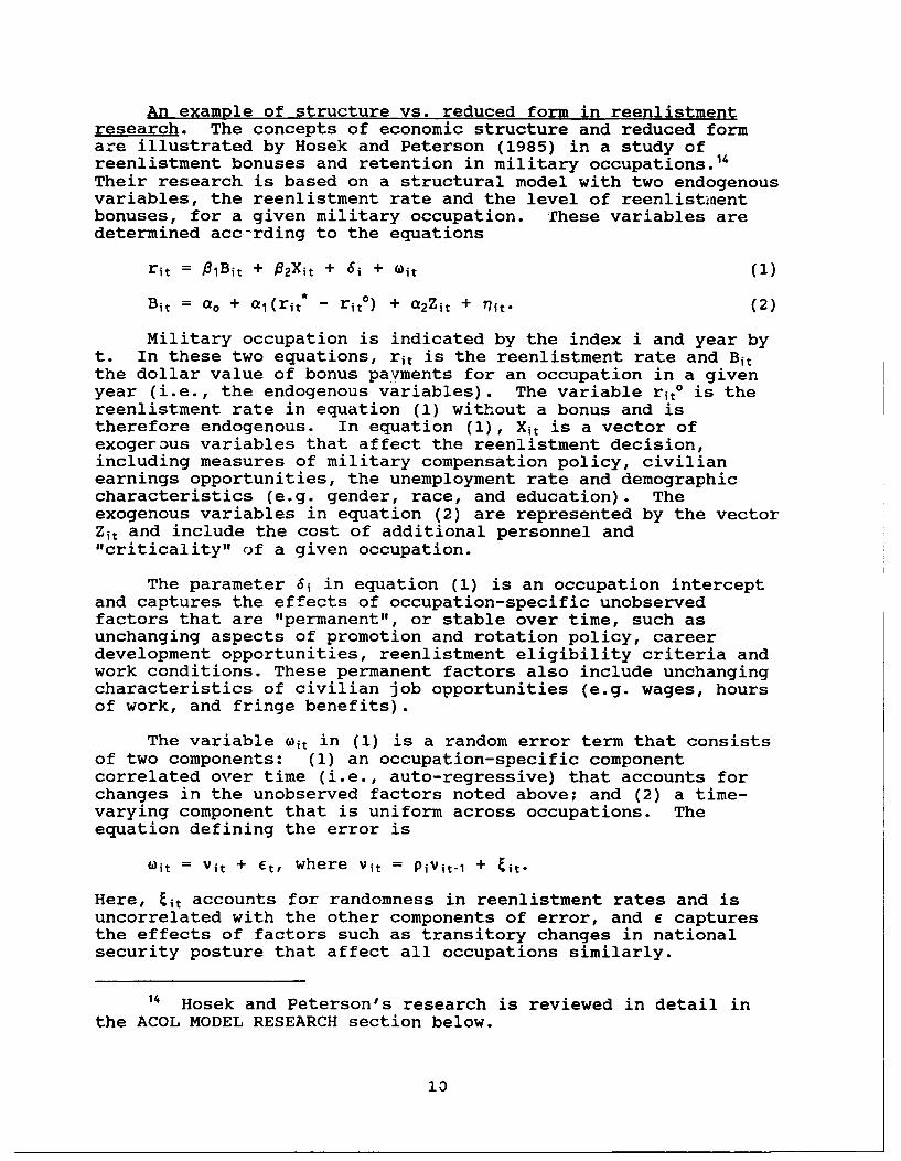
An example of structure vs. reduced form in reenlistmentresearch. The concepts of economic structure and reduced formare illustrated by Hosek and Peterson (1985) in a study ofreenlistment bonuses and retention in military occupations."Their research is based on a structural model with two endogenousvariables, the reenlistment rate and the level of reenlistmentbonuses, for a given military occupation. These variables aredetermined acc-rding to the equations

rit = PlBit + 02Xit + 6i + wit (1)

Bit = ao + al(rit* - rit ° ) + a2Zit + flit. (2)

Military occupation is indicated by the index i and year byt. In these two equations, rit is the reenlistment rate and Bitthe dollar value of bonus payments for an occupation in a givenyear (i.e., the endogenous variables). The variable rit* is thereenlistment rate in equation (1) without a bonus and istherefore endogenous. In equation (1), Xit is a vector ofexogerous variables that affect the reenlistment decision,including measures of military compensation policy, civilianearnings opportunities, the unemployment rate and demographiccharacteristics (e.g. gender, race, and education). Theexogenous variables in equation (2) are represented by the vectorZit and include the cost of additional personnel and"criticality" of a given occupation.

The parameter 6i in equation (1) is an occupation interceptand captures the effects of occupation-specific unobservedfactors that are "permanent", or stable over time, such asunchanging aspects of promotion and rotation policy, careerdevelopment opportunities, reenlistment eligibility criteria andwork conditions. These permanent factors also include unchangingcharacteristics of civilian job opportunities (e.g. wages, hoursof work, and fringe benefits).

The variable wit in (1) is a random error term that consistsof two components: (1) an occupation-specific componentcorrelated over time (i.e., auto-regressive) that accounts forchanges in the unobserved factors noted above; and (2) a time-varying component that is uniform across occupations. Theequation defining the error is

wit = vit + e, where vit = pivit-i + tit.

Here, Eit accounts for randomness in reenlistment rates and isuncorrelated with the other components of error, and e capturesthe effects of factors such as transitory changes in nationalsecurity posture that affect all occupations similarly.

14 Hosek and Peterson's research is reviewed in detail in

the ACOL MODEL RESEARCH section below.

13

In equation (2), rit* is the reenlistment rate needed to meetmanning requirements for occupation i in period t, and nit is arandom error. Finally, the reenlistment rate without a bonus in(2) is the forecast for period t derived by setting Bit equal tozero equation in (1) which yields

rit' = P2Xit + 6i + Piit-1 (3)

The term Mit-i in equation (3) is defined as the residual betweenthe actual and predicted reenlistment rates for a given period(t-1 in this case).

Compensation policy determines occupation-specificreenlistment rates and the level of bonus payments in this model(i.e., the endogenous variables of the structure) in severalways. First, compensation and other personnel costs affect themagnitudes of the exogenous variables Xit and Zit directly.Defining skill "criticality" factors for occupations also affectsthe latter. Second, the selection of critically important MOS andthe definition of their manning requirements rit are the resultof military personnel policy decisions. Finally, the random errorterm in (1) is influenced by policy changes because it accountsfor unobserved policy effects on reenlistment rates.

If data are available to measure the variables and policyparameters defined for equations (1) and (2), the structuralreenlistment equation (i.e., (1)) can be estimated and used toforecast the impact of changes in SRB policy. An alternative isto estimate the reduced form of (1) and apply the results toevaluate changes in SRB policy. This approach is lesscomplicated than structural estimation because: (a) the detailedformulation of a structural model may be avoided, and (2) reducedforms depend only on exogenous variables and are therefore easierto estimate.

In general, the reduced form of a structural equation can beformulated and estimated without knowledge of structure. Areduced form equation can therefore be determined without knowinghow changes in policy affect the structure of economic decisionmaking. Under this circumstance, the effects of policy changeson the parameters of a reduced form will also be unknown. Theexample below demonstrates that application of a reduced formmodel in this context can result in erroneous forecasts of policyeffects.

The reduced form of the reenlistment equation (1) is derivedas follows: (1) substitute equation (3) for rit° in (2) and solvefor Bit as a function of the exogenous variables Xit and Zi., and(2) insert the result in (1). The reduced form of (1) is

rit = (aO + alrit*)Pl + (1 - Cf1P1)j 2Xt + 12IZit (4)

+ flinit - flicPigit-i + wit-

11

Equation (4) can be estimated by fitting reenlistment ratesfor given MOS to data measuring the exogenous variables Xit andZit, a constant term and an appropriately specified random errorterm. Forecasts of reenlistment rates can be derived forparticular MOS provided SRB policy remains unchanged. Supposehowever the Army reduces the required manning level rit* for agiven occupation as part of a broader manpower policy objectiveof downsizing the enlisted force. This change in policy causes a*

shift in the constant term, (ao + airit)PI, in (4). Forecasts ofreenlistment rates based on the "old" reduced form are thereforesubject to forecast error.

Another important research question concerns potentialsources of bias. Self selection occurs if soldiers who reenlistdiffer from soldiers who separate, and these differences areunobserved and constant over time. Failure to account forsuch differences may result in estimates of the effects ofmilitary compensation that are inaccurate.

The interaction between reenlistment bonuses and thereenlistment decision may also result in biased estimates of theeffects of bonuses on reenlistment rates. Higher SRBs areexpected to increase reenlistment rates. At the same time,selective reenlistment bonus policy targets increased bonuspayments to critical shortage MOS. Estimation of the effects ofSRB payments proceeds by comparing different levels of bonuspayments with corresponding reenlistment rates. Unless the useof reenlistment bonus policy is accounted for in the analysis,estimates of SRB effects may be too low (i.e., biased downward)compared to their actual impact.

The Dynamic Retention Model (DRM), the Annualized Cost ofLeaving Model (ACOL) and the ACOL-2 model, a recent extension ofthe ACOL model, are structural models that depart from theapproach of previous research.16 However, the development ofthese models from the economic theory of occupational choice isnot thoroughly discussed in the literature. Such a discussion is

15 Lee (1976) and Heckman (1976) independently undertookeconometric analyses of self-selection. Maddala (1983) surveyseconometric research on selection bias. Recent developmentsinclude the application of duration models in analyses oflongitudinal data. See for example Heckman and Singer (1986).

16 The DRM preceded the ACOL model. The latter was in

fact, derived from the former. See Warner (1979) for the firstdescription and application of the ACOL model, and a discussionof its origins. Research involving the development andapplication of the DRM and ACOL models has focused on theinstitutional aspects of compensation policy. ACOL-2 researchshifts attention to the importance of structure and theresolution of structural issues.

12

needed and is important for two reasons. First, it providesinformation that can be used by policy makers/analysts and otherresearchers to asses the effectiveness of alternative modelsavailable for analyses of reenlistment policy. Second, itidentifies areas of research that may improve the forecastingaccuracy of models of the reenlistment decision.

The next section describes a structural model of thereenlistment decision beginning with the economic theory ofoccupational choice. This is followed by a summary of the ACOLmodel and a review of research based on this model and analternative methodology. The section on the ACOL-2 modelexamines the second generation ACOL model. Finally, theimplications of this review for estimation of SRB effect fnrselected MOS are discussed in the last section.

THE ECONOMIC THEORY OF OCCUPATIONAL CHOICE

Willis and Rosen (1979) summarized the economic theory ofoccupational choice in the context of educational investments.17

The theory predicts that an individual will select thatoccupation providing the largest expected lifetime utility, orsatisfaction. This criterion is expressed in terms of thepresent value of monetary benefits of each alternative. Non-pecuniary differences between occupations are also incorporatedin the analysis to account for the effects of observed andunobserved individual tastes and family circumstances on theselection of an occupation.

For example, suppose an individual must select an occupationfrom n alternatives. Each occupation provides earnings duringthe time he/she is employed. The time dimension of earnings isignored initially to simplify the discussion. Let Y be potentiallifetime earnings for a given individual, indicated by the indexi, if occupation j is selected, where

Yij = yj (Xi, Ti) (5)

Here Xi includes observed ability indicators and socioeconomicfactors (e.g., race, gender, education, experience) that affectthe individual's lifetime earnings, and ri represents unobservedcomponents of ability.

The value of choosing occupation j is the value now, orpresent value, of expected future earnings and non-pecuniarybenefits in that occupation. Present value is defined accordingto

Vii = g(Yij, zi, 1) (6)

17 The general theory of human capital is developed by

Becker (1975) and Mincer (1974).

13

where zi represents observed individual taste and familybackground factors, and Ai captures unobserved taste and familybackground effects. Equation (6) translates expected futureearnings into present value and is conditioned on taste andfamily background effects.

In this model, a given individual selects that occupationwith the highest present value, Vi*, where

Vi* = max (Vil, Vi2 , ... , Vin) (7)

The model also incorporates the assumption that unobservedindividual and family effects, ri and As0 are distributed amongindividuals according to the distribution function

F(7-iAi) (8)

A structural model of the decision to reenlist in the Armyis derived from equations (5) - (8) as follows. The value ofstaying in the Army, VAi, is the present value of: (1) militarycompensation, (2) civilian earnings after separation orretirement from the army, and (3) the value of non-pecuniarybenefits. From equation (6), this present value is definedaccording to

VAi = g(YAi, zi, A) (9)

where YAi is expected earnings over time if a soldier reenlists.Similarly, Vcj, the present value of civilian occupations thatare alternatives to the Army, is defined as

VCi = g(Yci, zi, A) (10)

where Yci is expected lifetime earnings if a soldier leaves theArmy and enters a civilian occupation instead.

Equation (7) implies that an individual will reenlist in theArmy if and only if VAj > Vci. Otherwise he/she will separateimmediately and enter a civilian occupation (i.e., if Vci > VAj).The selection criteria in this model are defined in terms ofprobabilities (Pr)

Pr(reenlist in the Army) = Pr (VAi > Vcj) (11)

Pr(separate from the Army) = Pr (VAi : Vcj) (12)

Stochastic assumptions (i.e., regarding random or non-parametric errors) and key features of military compensation needto be added to the model represented by equations (5)-(8) tocomplete the specification of a structural reenlistment model.Both issues are addressed by translating equations (9) and (10)into empirical definitions of the present value of the incomestreams for staying in and leaving the Army, respectively. In

14

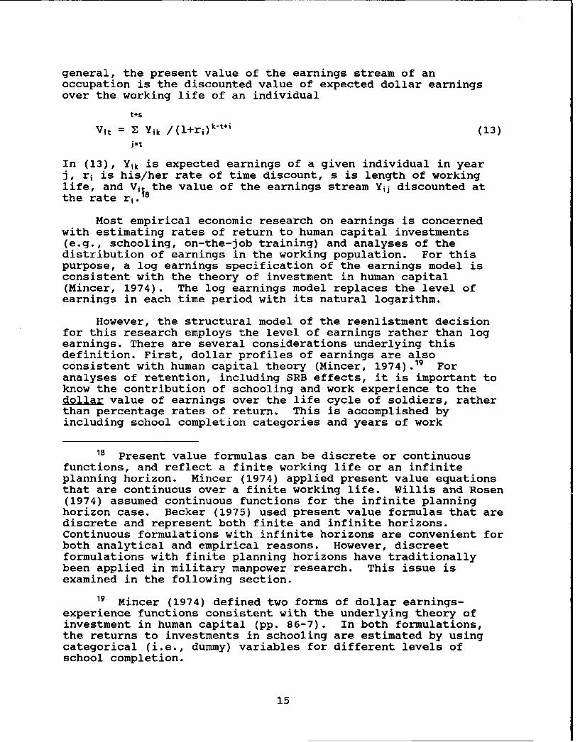
general, the present value of the earnings stream of anoccupation is the discounted value of expected dollar earningsover the working life of an individual

t S

Vit = Z Yik /(l+ri)k-t+ (13)j=t

In (13), Yik is expected earnings of a given individual in yearj, ri is his/her rate of time discount, s is length of workinglife, and Vil the value of the earnings stream Yij discounted atthe rate ri.

Most empirical economic research on earnings is concernedwith estimating rates of return to human capital investments(e.g., schooling, on-the-job training) and analyses of thedistribution of earnings in the working population. For thispurpose, a log earnings specification of the earnings model isconsistent with the theory of investment in human capital(Mincer, 1974). The log earnings model replaces the level ofearnings in each time period with its natural logarithm.

However, the structural model of the reenlistment decisionfor this research employs the level of earnings rather than logearnings. There are several considerations underlying thisdefinition. First, dollar profiles of earnings are alsoconsistent with human capital theory (Mincer, 1974). 19 Foranalyses of retention, including SRB effects, it is important toknow the contribution of schooling and work experience to thedollar value of earnings over the life cycle of soldiers, ratherthan percentage rates of return. This is accomplished byincluding school completion categories and years of work

18 Present value formulas can be discrete or continuousfunctions, and reflect a finite working life or an infiniteplanning horizon. Mincer (1974) applied present value equationsthat are continuous over a finite working life. Willis and Rosen(1974) assumed continuous functions for the infinite planninghorizon case. Becker (1975) used present value formulas that arediscrete and represent both finite and infinite horizons.Continuous formulations with infinite horizons are convenient forboth analytical and empirical reasons. However, discreetformulations with finite planning horizons have traditionallybeen applied in military manpower research. This issue isexamined in the following section.

19 Mincer (1974) defined two forms of dollar earnings-experience functions consistent with the underlying theory ofinvestment in human capital (pp. 86-7). In both formulations,the returns to investments in schooling are estimated by usingcategorical (i.e., dummy) variables for different levels ofschool completion.

15

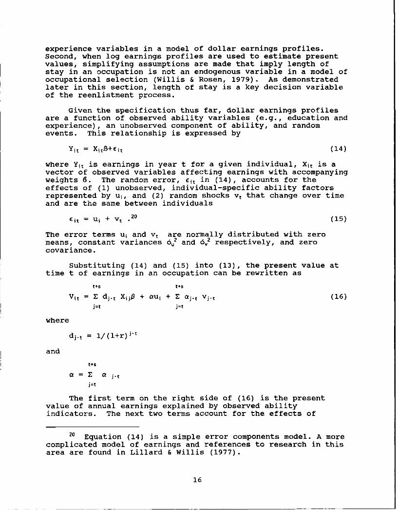
experience variables in a model of dollar earnings profiles.Second, when log earnings profiles are used to estimate presentvalues, simplifying assumptions are made that imply length ofstay in an occupation is not an endogenous variable in a model ofoccupational selection (Willis & Rosen, 1979). As demonstratedlater in this section, length of stay is a key decision variableof the reenlistment process.

Given the specification thus far, dollar earnings profilesare a function of observed ability variables (e.g., education andexperience), an unobserved component of ability, and randomevents. This relationship is expressed by

Yit = XitB+Eit (14)

where Yit is earnings in year t for a given individual, Xit is avector of observed variables affecting earnings with accompanyingweights B. The random error, Eit in (14), accounts for theeffects of (1) unobserved, individual-specific ability factorsrepresented by ui, and (2) random shocks vt that change over timeand are the same between individuals

Cit = ui + vt .20 (15)

The error terms ui and vt are normally distributed with zeromeans, constant variances 6u2 and 6V2 respectively, and zerocovariance.

Substituting (14) and (15) into (13), the present value at

time t of earnings in an occupation can be rewritten as

t+s t+s

Vit= dj-t XjjP + aui + Z aj-t vj-t (16)j=t j=t

where

dj t = i/(l+r)j-t

and

t+s

a a j-t

j=t

The first term on the right side of (16) is the presentvalue of annual earnings explained by observed abilityindicators. The next two terms account for the effects of

20 Equation (14) is a simple error components model. A more

complicated model of earnings and references to research in thisarea are found in Lillard & Willis (1977).

16

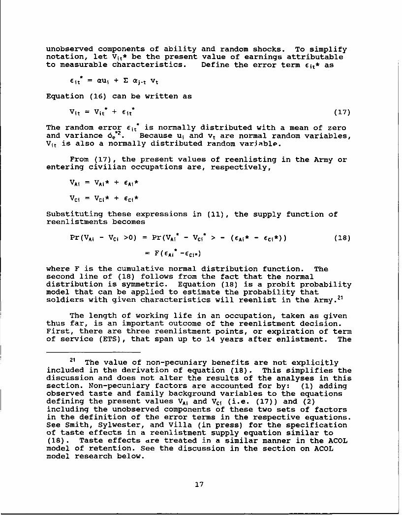
unobserved components of ability and random shocks. To simplifynotation, let Vit* be the present value of earnings attributableto measurable characteristics. Define the error term cit* as

*

Eit = Gui + E Zj-t vt

Equation (16) can be written as

Vit = Vit* + fit* (17)

The random error fit is normally distributed with a mean of zeroand variance 6e2 . Because ui and vt are normal random variables,Vit is also a normally distributed random variable.

From (17), the present values of reenlisting in the Army orentering civilian occupations are, respectively,

VAi = VAi* + EAi*

Vci = Vci* + eCi*

Substituting these expressions in (11), the supply function ofreenlistments becomes

Pr(VA, - Vci >0) = Pr(VAi* - Vci* > - (eAi* - CCi*)) (18)

F(EAi* -EC*)

where F is the cumulative normal distribution function. Thesecond line of (18) follows from the fact that the normaldistribution is symmetric. Equation (18) is a probit probabilitymodel that can be applied to estimate the probability thatsoldiers with given characteristics will reenlist in the Army.2'

The length of working life in an occupation, taken as giventhus far, is an important outcome of the reenlistment decision.First, there are three reenlistment points, or expiration of termof service (ETS), that span up to 14 years after enlistment. The

21 The value of non-pecuniary benefits are not explicitly

included in the derivation of equation (18). This simplifies thediscussion and does not alter the results of the analyses in thissection. Non-pecuniary factors are accounted for by: (1) addingobserved taste and family background variables to the equationsdefining the present values VAi and Vci (i.e. (17)) and (2)including the unobserved components of these two sets of factorsin the definition of the error terms in the respective equations.See Smith, Sylwester, and Villa (in press) for the specificationof taste effects in a reenlistment supply equation similar to(18). Taste effects are treated in a similar manner in the ACOLmodel of retention. See the discussion in the section on ACOLmodel research below.

17

first ETS date occurs between 2 and 6 years of service. Thesecond and third ETS dates take place in the intervals 6-10 and11-14, respectively. When soldiers reenlist, they select alength of service obligation within the relevant ETS interval.Retirement is a second feature of the Army's personnel systemthat makes length of service an important decision variable. Asoldier must stay in the Army at least 20 years to receiveretirement benefits. The value of expected retirement paydepends on the personal discount rate ri. If this rate isrelatively low (e.g., less than 10 percent), retirement benefitswill be given greater value than if ri is relativelyhigh.Soldiers with lower discount rates are therefore more likelyto reenlist and make the Army a career than those with higherdiscount rates.

An early attempt to formulate a structural model of themilitary reenlistment decision was the ACOL model. It isexamined below and compared to the model described in thissection. Research that has applied the ACOL model to estimatesupply elasticities for military occupations is summarized next.Other evaluations of the effects of SRBs are included in thisdiscussion. The ACOL-2 model, a recent extension and improvementof the ACOL model, is described in the following section. Theimplications of this review for analyses of the impact of SRB'sare discussed in the final section.

ACOL MODEL RESEARCH

The ACOL Model

The ACOL model evaluates the Cost of leaving the militaryfor addtitonal years of active duty service. Warner (1979)developed the initial specification of the ACOL model in analysesof the military retirement system. Recently, several versions ofthe model have been applied across the services to a variety ofcompensation policy issues. The essential elements of the modelare described as follows.22 A given soldier eligible toreenlist according to Army standards can either stay for anadditional period of time or leave and enter a civilianoccupation. Let RS (s) be the present value of the expectedincome stream at time t if the soldier stays in the Army s moreyears (VA in (9)). Similarly, let RL be the present value ofincome expected over time if the soldier leaves the Army at timet (Vc1 in (10)). The returns to staying, RS(s), are the sum of(1) the present value (at time t) of expected active duty pay fors more periods (2) the present value of retirement benefits (ifany) that would begin in period t+s, and (3) the present value ofexpected civilian earnings after s additional years in the Army.The returns to leaving at t are: (1) the present value of

22 The notation and variable definitions in this sectionare in Black et al. (1987), Appendix A.

18

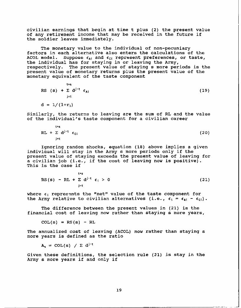
civilian earnings that begin at time t plus (2) the present valueof any retirement income that may be received in the future ifthe soldier leaves immediately.

The monetary value to the individual of non-pecuniaryfactors in each alternative also enters the calculations of theACOL model. Suppose EAi and eci represent preferences, or taste,the individual has for staying in or leaving the Army,respectively. The present value of staying s more periods is thepresent value of monetary returns plus the present value of themonetary equivalent of the taste component

t+s

RS (s) + Z di-t EAi (19)

j=t

d = 1/(l+r)

Similarly, the returns to leaving are the sum of RL and the valueof the individual's taste component for a civilian career

t+s

RL + Z di-t Eci (20)j=t

Ignoring random shocks, equation (18) above implies a givenindiviaual will stay in the Army s more periods only if thepresent value of staying exceeds the present value of leaving fora civilian job (i.e., if the cost of leaving now is positive).This is the case if

t+s

RS(s) - RL + Z di-t Ei > 0 (21)j=t

where ei represents the "net" value of the taste component forthe Army relative to civilian alternatives (i.e., eC = EAi - EC)-

The difference between the present values in (21) is thefinancial cost of leaving now rather than staying s more years,

COL(s) = RS(s) - RL

The annualized cost of leaving (ACOL) now rather than staying smore years is defined as the ratio

A, = COL(s) / E di-t

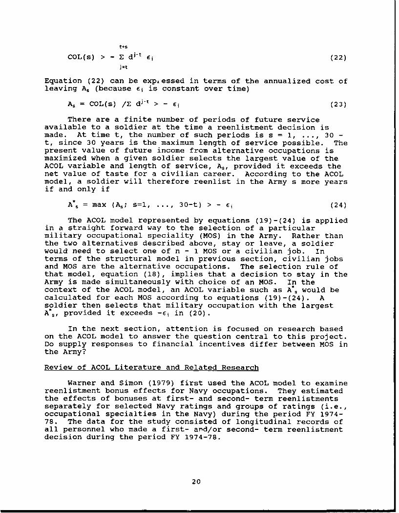
Given these definitions, the selection rule (21) is stay in theArmy s more years if and only if

19

t+s

COL(s) > - E dj't Ei (22)j=t

Equation (22) can be expiessed in terms of the annualized cost ofleaving A, (because Ei is constant over time)

As = COL(s) /E dj-t > - Ei (23)

There are a finite number of periods of future serviceavailable to a soldier at the time a reenlistment decision ismade. At time t, the number of such periods is s = 1, ..., 30 -t, since 30 years is the maximum length of service possible. Thepresent value of future income from alternative occupations ismaximized when a given soldier selects the largest value of theACOL variable and length of service, A,, provided it exceeds thenet value of taste for a civilian career. According to the ACOLmodel, a soldier will therefore reenlist in the Army s more yearsif and only if

A% = max (A,; s=l, ... , 30-t) > - ci (24)

The ACOL model represented by equations (19)-(24) is appliedin a straight forward way to the selection of a particularmilitary occupational speciality (MOS) in the Army. Rather thanthe two alternatives described above, stay or leave, a soldierwould need to select one of n - 1 MOS or a civilian job. Interms of the structural model in previous section, civilian jobsand MOS are the alternative occupations. The selection rule ofthat model, equation (18), implies that a decision to stay in theArmy is made simultaneously with choice of an MOS. In thecontext of the ACOL model, an ACOL variable such as A*% would becalculated for each MOS according to equations (19)-(24). Asoldier then selects that military occupation with the largestA*9, provided it exceeds -Ei in (20).

In the next section, attention is focused on research basedon the ACOL model to answer the question central to this project.Do supply responses to financial incentives differ between MOS inthe Army?

Review of ACOL Literature and Related Research

Warner and Simon (1979) first used the ACOL model to examinereenlistment bonus effects for Navy occupations. They estimatedthe effects of bonuses at first- and second- term reenlistmentsseparately for selected Navy ratings and groups of ratings (i.e.,occupational specialties in the Navy) during the period FY 1974-78. The data for the study consisted of longitudinal records ofall personnel who made a first- and/or second- term reenlistmentdecision during the period FY 1974-78.

20

A probit model was estimated that included alternativemeasures of the ACOL variable, fiscal year dummy variables (i.e.,variables with a value of 1 or 0), marital status, and in somecases, education and race variables. In an effort to account fora changing distribution of taste for Navy life, the first-termreenlistment bonus was included as a variable in second-termreenlistment equations. The estimated effect of a one unitincrease in the bonus multiplier at first-term reenlistmentranged from 1.7 to 5.1 additional reenlistments per 100 eligibleNavy personnel. The estimated effect of a one unit change in thebonus multiplier on second-term reenlistment rates were similar.The effect of first-term bonuses on second-term reenlistmentrates was consistently negative as expected.

Goldberg & Warner (1982) applied another version of the ACOLmodel to assess the impact of reenlistment bonuses and regularmilitary compensation on reenlistments and extensions across Navyratings during FY 1974-80. Using data grouped by fiscal year,Navy rating and length of service, they estimated multinomiallogit models of reenlistments and extensions for first- andsecond-term reenlistments separately. They found that the effectof a one level increase in SRB multipliers increasedreenlistments at the first term point from 1.7 to 3.3 persons perhundred eligible to reenlist and 1.9 to 6.0 persons at the secondterm.

A measure of the incidence of shore duty was included in thefirst term and second term equations to determine whetherreenlistment rates were relatively lower for ratings thatrequired more time at sea. The results for this variable weremixed, although the majority of the estimates were negative andstatistically significant. Following Warner and Simon (1979),Goldberg and Warner (1982) also included actual (average) SRBpayments received at first-term reenlistment as a variable in thesecond term equations. The results for this variable wereinconclusive.

Neither version of the ACOL model described above explainswhy pay elasticities, including SRB effects, are expected todiffer between occupations. In a subsequent study, Warner andGoldberg (1984) developed an ACOL model where differential payeffects are a consequence of the role of non-pecuniary factors inthe reenlistment decision process. In their model, the tasteparameters for civilian and military occupations, respectively,are assumed to be normally distributed, unobserved randomvariables. The effects of non-pecuniary factors on reenlistmentsupply elasticities are captured by the variances of theseunderlying taste distributions. The principle implicationsconcerning supply elasticities are:

1. Peenlistment supply will be more elastic with respect topay if there is no correlation between taste for militaryand civilian occupations, and the dispersion of tastefactors in the population is small.

21

2. The greater the correlation in taste between occupationsin military and civilian jobs, the more easily occupationsin the two sectors can be substituted for one another. Thismeans that small changes in military compensation will leadto relatively large increases in reenlistment rates.Conversely, small changes in civilian earnings will inducerelatively large reductions inreenlistment rates.

3. The primary non-pecuniary factor present among Navyratings is the incidence of sea duty, measured by theproportion of time spent at sea. Warner and Goldberg (1984)demonstrated that reenlistment supply was more inelasticwith respect to pay the greater this ratio. In terms of theArmy, comparable non-pecuniary factors would include degreeof risk (e.g., combat arms) and location of duty station(CONUS vs OCONUS). For example, combat arms MOS (lIB - 19E)and MOS that involve overseas duty stations are expected tobe less responsive (i.e., less elastic) to reenlistmentbonuses and other forms of military compensationrelative to other MOS.

In their empirical analyses, Warner and Goldberg (1984)focused on Navy personnel who made a first-term reenlistmentdecision during the period FY 1974-78. Approximately 80 enlistedoccupations were reclassified into 16 occupational categories.The proportion of enlisted personnel assigned to sea duty variedbetween occupational groups from a low of 6.3% to 69.8%.Separate probit models of reenlistment were estimated for each ofthe 16 occupational groups. The estimated increase inreenlistment rates from a 1 unit increase in SRB multipliersranged from 1.8 to 5.5 persons per hundred eligible to reenlist.The results also support the hypothesis that a higher incidenceof sea duty is associated with lower supply elasticities. Thecorrelation between the percentage of personnel assigned sea dutyand estimated pay effects, -.49, was statistically significant atthe 5% level.

None of the research reported above accounted for the effectof simultaneous equation bias discussed earlier. This issuearises because there is interaction between reenlistment ratesand selective reenlistment bonuses. When selective reenlistmentbonuses increase in an MOS, the returns to staying relative toother MOS and civilian jobs increase, causing the annualized costof leaving to rise. Soldiers in an MOS (and possibly other MOSas well) on the margin of reenlisting who would have left theArmy in the absence of the SRB, will stay. For these soldiers,higher values of ACOL exceed the value they place on taste forcivilian employment. On the other hand, the Army systematicallyallocates reenlistment bonuses to increase reenlistments incritically important MOS that are below target force levels.Consequently, estimates of the effects of SRBs on reenlistmentrates will be based on data that include low reenlistment ratesassociated with high SRB's. As noted earlier, this tends to biasthe estimate of the average SRB effect downward.

22

Hosek and Peterson (1985) address the simulteneous equationbias issue in a study that compares the effects o± annualized vs.lump sum reenlistment bonuses. They do this by controlling forthe effects of unobserved factors on reenlistments. First, eachmilitary occupation (i.e., Army MOS) has its own intercept termin their model. The intercept accounts for the effects ofunobserved factors that are fixed over time. These factorsinclude the unchanging aspects of work conditions in the MOS,promotion policy, reenlistment eligibility criteria, rotationpolicy and career development opportunities. The effects ofunchanging aspects of civilian jobs that are alternatives forpersonnel in the MOS, such as wages, hours of work, etc., arealso accounted for by the intercept. Secondly, the error term inHosek and Peterson's model has two components. The firstcomponent is an occupat ion-specific first order autoregressiveerror. It represents the effects of the unobserved factorsdescribed above that do change over time. The second componentallows for the effect of transitory changes that affect all MOSequally. Examples of the latter are an unexpected threat tonational security and changes in military compensation that wouldaffect all services and military occupations alike.

Other variables include a military/civilian wage index(rather than an ACOL variable), an indicator of the presence of abonus in a MOS, bonus amount, national unemployment rate, percentof males without a high school diploma and percent black. Thebonus presence and amount variables are multiplied by a factordefined as one if the time period was after April 1, 1979 tocompare the effects of lump sum vs. annual installments onreenlistments. Logit models were estimated for reenlistments,extensions and retention. Retention was defined as theoccurrence of either a reenlistment or an extension. The modelswere estimated using data consisting of cell means for allmilitary occupational specialties in the Army, Navy, and AirForce during the period FY 76-81.

An important implication of Hosek and Peterson's (1985)model is that if reenlistment bonuses are targeted so that theyare higher for "critical shortage" MOS, the inclusion ofoccupation intercepts and removal of intertemporal correlationfrom the error term controls for simultaneous equation bias.Therefore it would be reasonable to expect estimates ofreenlistment bonus effects based on this specification to exceedestimates derived from a model that excludes an occupationintercept and/or fails to remove auto-correlation from the errorterm. The results of the study confirm this hypothesis. Theestimated effect of reenlistment bonuses for first-termreenlistments was .0173 when simultaneity was ignored. Thisestimate increased significantly to .0759, however, whenoccupation intercepts were added to control for permanent fixedeffects. The addition of the auto-correlated error disturbancesto account for the influence of time varying unobserved factorshad little effect on the estimates.

23

THE SECOND GENERATION ACOL (ACOL-2) MODEL

The preceding discussion of ACOL research raises importantissues about the specification of the ACOL model as a structuraleconomic model. First, the stochastic assumptions of the ACOLmodel do not provide adequate control for the influence ofunobserved population heterogeneity. Consequently, estimates ofeffects of policy variables may be biased. Furthermore, the ACOLmodel incorporates incomplete knowledge about the effects ofchanges in defense policy and Army personnel policy on thestructure of the reenlistment decision. These specificationproblems may reduce the forecasting accuracy of the ACOL modeland its usefulness as a policy evaluation tool.

Unobserved heterogeneity is included in the ACOL model asthe source of random error in the earnings and cost of leavingequations. The selection rule of the model, equation (24),implies that a soldier will reenlist if the net cost of leaving(the value of expected military compensation less the value ofexpected civilian income) exceeds the monetary equivalent valueto him/her of net (unobserved) taste for civilian life. The costof leaving measures the pecuniary or financial cost of leaving toan individual. The value of net taste for civilian life on theother hand is the monetary value of non-pecuniary benefits ofcivilian relative to Army life. Given the financial cost ofleaving, the smaller the non-pecuniary benefits of civilianrelative to Army life, the more likely it is that a soldier willstay in the Army. Alternatively, given the cost of leaving(ACOL) the greater the preference for Army life, the higher isthe probability soldiers will reenlist. Thus, the presence ofunobserved heterogeneity means that for an enlistment cohort,soldiers eligible to reenlist who decide to stay at their firstreenlistment decision point are those with greater preferencesfor Army life than soldiers who leave.

As length of service increases the value of the ACOLvariable tends to rise because of retirement pay. Thedistribution of unobserved preferences for Army life also changesover time. In particular, at the 2nd ETS, the average value ofunobserved taste factors will increase for soldiers who reenlista second time. Differences in taste also become smaller (i.e.,the variance of the taste distribution declines) as soldiersbecome more homogeneous in terms of their preferences. Thedistributional changes outlined here combined with rising ACOLvalues imply that the probability of reenlistments will increaseover time. Thus, the probability of reenlistment at the secondETS is expected to be higher than at the first ETS. A similarconclusion follows comparing the second and third reenlistments.

The specification of the random error term in the ACOL modeldoes not capture the notion of a changing taste distribution asdescribed here. One consequence is that the model does notaccurately predict reenlistment rates after the first ETS. Asecond issue is that estimates of the effect of the ACOL variable

24

derived from the model are biased upward. Consider first, theselection rule, equation (24). By assumption, the error term ciis constant over time. Furthermore, as indicated above, thevalue of ACOL tends to rise with length of service.Consequently, the value of As* at the second reenlistmentdecision print, call it A2 , will be greater than ACOL at thefirst reenlistment, A,*. The ACOL model, therefore, predicts(i.e., see equation (24)) that all soldiers who reenlisted thattheir first ETS will also reenlist at their second ETS. That is,it predicts a reenlistment rate of one.

Observed reenlistment rates after the first ETS, thoughhigh, are significantly less than one. The source of thisspecification problem is that the error term in (24) consists ofonly a permanent fixed component. Thus, soldiers do not revisetheir assessments of the value of non-pecuniary factors over timeaccording to the ACOL model.23 This problem can be corrected byincluding a random shock, or transitory, error component thatfluctuates randomly over time. Such a component representschanges in non-pecuniary factors and other unobserved variablesthat may influence reenlistments. This issue is examined indetail in the discussion of the ACOL-2 model below.

Warner (1979), Warner and Simon (1979), and Goldberg andWarner (1982) acknowledged the potential for bias attributable tounobserved differences and included the value of first termreenlistment bonuses as a variable in second term reenlistmentequations. This approach did not however adequately address theheterogeneity issue. Estimation of reenlistment supply functionsbased only on data for soldiers at a specific ETS (e.g., Warnerand Simon) ignores selectivity by implicitly assuming that theerror term is normally distributed with a mean of zero and aconstant variance for that ETS decision point.

Another issue raised by the specification of the ACOL modelconcerns how policy changes are incorporated in a structuralmodel of reenlistments. For example, consider the effects of ageneral increase in selective reenlistment bonuses. As the valueof the ACOL variable increases, soldiers with relatively lesstaste for Army life will reenlist rather than leave. If firstterm bonuses are not maintained for the second reenlistmentdecision, however, ACOL values will decline (relative to theirvalues at the first ETS) and second term reenlistment rates fallas soldiers with relatively less taste for Army life leave. Ingeneral, changes in compensation policy affect reenlistment ratesby changing the relative benefits of the Army as an occupation,and changing the distribution of unobserved taste for Army life.

23 See Smith, Sylwester, and Villa (in press) for an

analysis of this issue. The specification of the error term inthe ACOL model does not allow standard methods of estimation tobe applied to the multiple decision process of reenlistment.

25

Therefore, for policy evaluation purposes a structural economicmodel of the reenlistment decision must address the issue ofheterogeneity in a multiple stay-leave environment. Thepreceding discussion demonstrates that the ACOL model does not dothis.

A fourth issue is the selection of probability models usedto estimate the probability of reenlistments. Much of the ACOLresearch (as well as other military manpower research) has reliedon the logit probability model for reasons of computationalconvenience and cost. However, empirical research on dollarearnings and log earnings profiles has traditionally hypothesizednormally distributed error terms. The earlier discussionindicates that under this circumstance, the probit probabilitymodel is the appropriate model for analyses of the reenlistmentdecision. 24

Recent research has extended the ACOL framework to addressthe problem of unobserved heterogeneity. Black, Hogan andSylwester (1987) developed the ACOL-2 model for analysis ofreenlistment in the Navy. This model is an error componentsprobit model that predicts the probability of reenlistment basedon estimates derived from longitudinal data. Self selection iscontrolled by specifying an error term with two components. Onecomponent represents the effect of heterogeneity of taste formilitary service. The second component reflects the impact oftransitory changes on the value of non-pecuniary factors for theArmy and civilian occupations. Data for the study were obtainedfrom annual enlisted master files for first-term ETS cohorts inFY 75, FY 77, FY 79 and FY 81. These annual files were linked toconstruct longitudinal records that traced each individual'scareer in the Navy through 30 June 1985.

As the objective of the research was to evaluate theinformation gains of the ACOL-2 model relative to the ACOL model,a conventional ACOL model was also estimated using thelongitudinal database. Each model included an ACOL variable,Armed Forces Qualifying Test (AFQT) score, date of entry into theNavy, Navy occupational group (groups of Navy ratings), gender,race, education and number of dependents. Variables for 2nd and3rd ETS and years of service (YOS) entered some models as

24 The method for computing the ACOL variable in research

based on the ACOL and more recent ACOL-2 and other methodologiesraises a specification issue. Earnings profiles are calculatedby transforming the log of earnings. Because log earnings arenormally distributed in this research, dollar earnings do notfollow a normal distribution. Section three demonstrates,however, that the probit probability model follows from thehypothesis that dollar earnings are normally distributed. Theempirical implications of this specification issue are unclear.

26

regressors to assess the effects of military experience onreenlistments.

The estimated impact of the ACOL variable ignoringheterogeneity indicated that for each $1000 increase in militarypay, the 1st term reenlistment rate increased by 1.7 percent.The estimate of ACOL in the ACOL-2 model which does control forunobserved heterogeneity, was .9 percent, approximately half aslarge as the conventional estimate. This difference clearlysuggests that the estimated impact of military pay in the ACOLmodel includes the impact of self selection, and thus overstatesthe effect of military pay.

An ad hoc procedure for controlling selection bias wasevaluated by including term of service and YOS variables in theACOL model. When these two sets of military experience variableswere entered separately and together as regressors, the estimatesof the effects of the ACOL variable were about .9, the same asthe ACOL-2 model. It appears that "YOS and ETS serve as proxiesfor the censoring of the taste distribution over successivereenlistment decisions." (Black et al., 1987, p. 5-10). Thisfinding appears to suggest that including experience-relatedvariables in the conventional ACOL model may provide adequatestatistical control for the effects of unobserved heterogeneity.

However, the ACOL model does not capture the effects ofpolicy changes on the structure of the reenlistment decisionprocess as noted previously. To illustrate this, Black et al.(1987) simulate policy alternatives by assuming reenlistmentbonuses increase at the 1st ETS in such a way that ACOL valuesrise by 50 percent. The ACOL-2 model predicts an increase of2.4% in reenlistments at the 1st ETS and a decrease of 1.3% and.5% at the 2nd and 3rd ETS. The ACOL model predicts a 2.1%increase at the 1st ETS and no change for subsequent ETS.

IMPLICATIONS

The purpose of this research is to examine key issues thatmust be addressed to reliably estimate the effects of SRBs onreenlistment rates in critical shortage MOS. First, evidencefrom recent economic research indicates that unobservedheterogeneity is an important factor affecting reenlistments andcan result in overestimates of the impact of financialincentives, including SRBs, on reenlistment rates. Second, thereis also evidence that reenlistments and reenlistment bonuses areinterrelated within specific military occupations. Unlesscorrected, this interaction may impart a downward bias inestimated bonus effects. Third, what characteristics of soldiersare important in estimating SRB effects (e.g. race/ethnicity,sex, mental category), and what is the most appropriate way toobtain these estimates at the MOS level?

The ACOL-2 model combined with longitudinal data controlsfor biased compensation effects due to population heterogeneity.

27

The simultaneous equation bias problem is also addressed byappropriate specification of the model's random error term. Inaddition, the ACOL-2 model provides a flexible approach forevaluating SRB effects for subgroups of soldiers in selected MOS.

28

References

Becker, G. (1975). Human capital (2nd ed.). Chicago:University of Chicago.

Black, M., Hogan,P., & Sylwester, S. (1987). Dynamic model ofreenlistment behavior (Congressional Budget Office, ContractNo. 85-0058). Arlington, VA: Systems Research andApplications Corp.

Department of Defense. (1987). Military compensation backgroundpapers (3rd ed.). Washington, DC: U.S. Government PrintingOffice.

Enns, J. H. (1977). Reenlistment bonuses and first-termretention (Report No. R-1935-ARPA). Santa Monica, CA: Rand

Goldberg, M., & Warner, J. T. (1982). Determinants of Navyreenlistment and extension rates (Report No. CRC 476).Alexandria, VA: Center For Naval Analyses.

Goldberger, A. (1964). Econometric theory. New York: JohnWiley & Sons.

Grubert, H., & Weiher, R. (1970). Navy reenlistments: The roleof pay and draft pressure. In Studies prepared for thePresident's Commission On All-Volunteer Force. Washington,DC: U.S. Government Printing Office.

Hausman, J. A., & Wise, D. A. (1978). A conditional probitmodel for qualitative choice: Discreet decisionsrecognizing interdependence and heterogeneous preferences.Econometrica, 46, 403-426.

Heckman, J. J. (1976). The common structure of statisticalmodels of truncation, sample selection, and limiteddependent variables and a simple estimator for such models.Annals of Economic and Social Measurement, 5, 475-492.

Heckman J. J., & Singer, B. (1986). Econometric analysis oflongitudinal data. In Z. Griliches & M. Intriligator(Eds.), Handbook of Econometrics (Vol. 3, pp. 1689-1763).New York: North Holland.

Hosek, J. R., & Peterson, C. (1985). Reenlistment bonuses andretention behavior (Report No. R-3199-MIL). Santa Monica,CA: Rand.

Kleinman, S. D., & Shugart, W. F. (1974). The effects ofreenlistment bonuses (Report No. CRC 269). Alexandria, VA:Center For Naval Analyses.

29

Lee, L. F. (1976). Estimation of limited dependent variablemodels by two stage methods. Unpublished doctoraldissertation, University of Rochester, Rochester, NY.

Lillard, L., & Willis, R. J. (1978). Dynamic aspects ofearnings mobility. Econometrica, 46, 985-1012.

Lucas, R. (1976). Econometric policy evaluation: A critique.In K. Brunner & A. Meltzer (Eds.), The Phillips curve andlabor markets, Carnegie-Rochester conference on publicpolicy, (Vol.1, pp. 19-46). New York: North Holland.

Maddala, G. S. (1983). Limited dependent and qualitativevariables in econometrics (Econometric Society monographsNo. 3). Cambridge: Cambridge University Press.

Marschak, J. (1953). Economic measurements for policy andprediction. In W. C. Hood & T. C. Koopmans (Eds.), Studiesin econometric method (pp. 1-26, Cowles Commission MonographNo. 14). New York: Wiley & Sons.

Mincer, J. (1974). Schooling, experience and earnings. NewYork: National Bureau of Economic Research.

Office of the Deputy Chief of Staff for Personnel. (1986, August28). Selective Reenlistment Bonus Decision Support System(SRB.DSS) Study Directive.

Nelson, G. R. (1970). Economic analysis of first-termreenlistments in the Army. In Studies prepared for thePresident's Commission On All-Volunteer Force. Washington,DC: U.S. Government Printing Office.

Smith, D. A., Sylwester, S., & Villa, C. (In preparation). Armyreenlistment models. In D. K. Horne, D. A. Smith, & C. L.Gilroy (Eds). Military compensation and personnelretention: models and evidence (Ch. 3). Alexandria, VA:U.S. Army Research Institute for the Behavioral and SocialSciences.

Taylor, J. B. (1986). Econometric approaches to stabilizationpolicy in stochastic models of macroeconomic fluctuations.In Z. Griliches & M. Intriligator (Eds.), Handbook ofeconometrics (Vol. 3, pp. 1997-2055). New York: NorthHolland.

Warner, J. T. (1979). Alternative military retirement systems:their effects on enlisted retention (Report No. CRC 376).Ajexandria, VA: Center For Naval Analyses.

30

Warner, J. T., & Goldberg, M. (1984). The influence ofnon-pecuniary factors and labor supply: The case of Navyenlisted personnel. Review of Economics and Statistics,66(l), 26-35.

Warner, J. T., & Simon, B. (1979). An empirical analysis of payand Navy enlisted retention in the AVF: Preliminaryresults. (Professional Paper No. 392). Alexandria, VA:Center For Naval Analyses.

Wilburn, R. C. (1970). Impact of income, the draft, and otherfactors in retention of Air Force enlisted men. In Studiesprepared for the President's Commission On All-VolunteerForce. Washington, DC: U.S. Government Printing Office.

Willis, R. J., & Rosen, S. (1979). Education and selfselection. Journal of Political Economy, 87(5,pt.2), S7-S36.

31