Embed Size (px)
DESCRIPTION
applied mathematics
Citation preview
Society for Industrial and Applied MathematicsPhiladelphia
MARINEACOUSTICS
Direct and Inverse Problems
James L. BuchananUnited States Naval Academy Annapolis, Maryland
Robert P. GilbertUniversity of Delaware Newark, Delaware
Armand WirginLaboratoire de Mécanique et d’AcoustiqueMarseille, France
Yongzhi S. XuUniversity of Tennessee at Chattanooga Chattanooga, Tennessee
OT84_fmA2.qxd 10/27/2004 3:52 PM Page 3
Copyright © 2004 by the Society for Industrial and Applied Mathematics.
10 9 8 7 6 5 4 3 2 1
All rights reserved. Printed in the United States of America. No part of this bookmay be reproduced, stored, or transmitted in any manner without the written permission of the publisher. For information, write to the Society for Industrialand Applied Mathematics, 3600 University City Science Center, Philadelphia, PA19104-2688.
Library of Congress Cataloging-in-Publication Data
Marine acoustics : direct and inverse problems / James L. Buchanan … [et al.].p. cm.
Includes bibliographical references and index.ISBN 0-89871-547-4 (pbk.)
1. Underwater acoustics. I. Buchanan, James L.
QC242.2.M37 2004620.2’5—dc22 2003070359
This research was supported in part by the National Science Foundation throughgrants BES-9402539, INT-9726213, BES-9820813, the Office of Naval Researchthrough grant N00014-001-0853, and the Centre National de la RechercheScientifique through grant NSF/CNRS-5932.
is a registered trademark.
OT84_fmA2.qxd 10/27/2004 3:52 PM Page 4
v This page has been reformatted by Knovel to provide easier navigation.
Contents
Preface ....................................................................................... xi
Acknowledgments ...................................................................... xii
1. The Mechanics of Continua ............................................... 1 1.1 Introduction ............................................................................. 1 1.2 Survey of Previous Work ........................................................ 5 1.3 Underlying Principles of the Mechanics of Continua .............. 9
1.3.1 Introduction ............................................................. 9 1.3.2 Lagrangian and Eulerian Coordinates, Deformation,
Strain, Displacement, and Rotation ......................... 10 1.3.3 Deformation Gradients and Deformation
Tensors ................................................................... 11 1.3.4 The Cauchy and Green Deformation Tensors ......... 12 1.3.5 Strain Tensors and Displacement Vectors .............. 13 1.3.6 Infinitesimal Strains and Rotations .......................... 15 1.3.7 Lagrangian and Eulerian Strains in the Framework
of Infinitesimal Deformations ................................... 16 1.3.8 Strain Invariants and Principal Directions ................ 17 1.3.9 Area and Volume Changes Due to Infinitesimal
Deformations ........................................................... 18 1.3.10 Kinematics .............................................................. 19 1.3.11 Material Derivatives of Line, Surface, and
Volume Integrals over Regions Devoid of Discontinuities ......................................................... 21
1.3.12 Material Derivatives of Integrals over Regions Containing a Discontinuity Surface .......................... 23
1.3.13 Conservation of Mass Law for Uniform Bodies ........ 24
vi Contents
This page has been reformatted by Knovel to provide easier navigation.
1.3.14 Conservation of Momentum and Energy Laws ........ 25 1.3.15 External and Internal Loads and Their Incorporation
in the Conservation of Momentum Equation ............ 25 1.3.16 Stress ...................................................................... 26 1.3.17 Global and Local Forms of the Conservation of
Momentum Law in Terms of Stress ......................... 27 1.3.18 Local Form of the Boundary Conditions on
Discontinuity Surfaces ............................................. 28 1.3.19 Thermodynamic Considerations .............................. 29 1.3.20 Constitutive Relations ............................................. 33
1.4 Mechanics of Elastic Media and Elastodynamics ................... 33 1.4.1 Definition of Elastic Media ....................................... 33 1.4.2 Constitutive Equations ............................................ 33 1.4.3 Linear Constitutive Equations (Linear Elasticity) ..... 37 1.4.4 Symmetry Properties of the Elastic Moduli
Tensor ..................................................................... 41 1.4.5 The Wave Equation for Elastodynamics in Linear
Elastic Media ........................................................... 42 1.4.6 Wave Equation for Elastodynamics in
Compressible, Homogeneous Materials .................. 43 1.4.7 Wave Equation for Elastodynamics in
Heterogeneous, Isotropic Solids .............................. 43 1.4.8 Wave Equation for Elastodynamics in
Homogeneous, Isotropic Solids ............................... 43 1.4.9 Obtaining the Wave Equation of Acoustics in
Heterogeneous, Inviscid Fluids from Navier’s Equation .................................................................. 45
1.4.10 Boundary Conditions between Two Linear, Isotropic, Homogeneous, Elastic Materials .............. 46
1.5 Forward and Inverse Wavefield Problems .............................. 48 1.5.1 Introduction ............................................................. 48 1.5.2 The Frequency-domain Equation for Propagation
in an Unbounded, Heterogeneous, Inviscid Fluid Medium ................................................................... 49

Contents vii
This page has been reformatted by Knovel to provide easier navigation.
1.5.3 The Frequency-domain Radiation Condition at Infinity ..................................................................... 50
1.5.4 Governing Equations for the Frequency-domain Formulation of Wave Propagation in an Unbounded, Heterogeneous, Inviscid Fluid Medium ................................................................... 51
1.5.5 Governing Equations for the Frequency-domain Formulation of Wave Propagation in Two Contiguous, Semi-infinite, Heterogeneous, Inviscid Fluid Media ................................................. 51
1.5.6 Governing Equations for the Frequency-domain Formulation of Wave Propagation in an Unbounded, Heterogeneous, Isotropic, Elastic Solid ........................................................................ 52
1.5.7 Governing Equations for the Frequency-domain Formulation of Wave Propagation in Two Semi-infinite, Heterogeneous, Isotropic, Elastic Solid Media in Welded Contact ........................................ 52
1.5.8 Governing Equations for the Frequency-domain Formulation of Wave Propagation in a Semi-infinite Domain Occupied by a Heterogeneous, Inviscid Fluid Contiguous with a Semi-infinite Domain Occupied by a Heterogeneous, Isotropic, Elastic Solid ............................................. 54
1.5.9 Eigenmodes of a Linear, Homogeneous, Isotropic Solid Medium of Infinite Extent ................. 55
2. Direct Scattering Problems in Ocean Environments ....... 57 2.1 The Constant Depth, Homogeneous Ocean .......................... 57
2.1.1 Point Source Response in a Constant Depth, Homogeneous Ocean ............................................. 57
2.1.2 Propagating Solutions in an Ocean with Sound-soft Obstacle ........................................................... 58
2.1.3 The Representation of Propagating Solutions ......... 59
viii Contents
This page has been reformatted by Knovel to provide easier navigation.
2.1.4 The Uniqueness Theorem for the Dirichlet Problem .................................................................. 61
2.1.5 An Existence Theorem for the Dirichlet Problem .................................................................. 66
2.1.6 Propagating Far-field Patterns ................................ 69 2.1.7 Density Properties of Far-field Patterns ................... 72 2.1.8 Complete Sets in L2(δΩ) .......................................... 72 2.1.9 Dense Sets in L2(δΩ) ............................................... 74 2.1.10 The Projection Theorem in VN ................................. 76 2.1.11 Injection Theorems for the Far-field Pattern
Operator .................................................................. 79 2.1.12 An Approximate Boundary Integral Method for
Acoustic Scattering in Shallow Oceans ................... 83 2.2 Scattered Waves in a Stratified Medium ................................ 92
2.2.1 Green’s Function of a Stratified Medium and the Generalized Sommerfeld Radiation Condition ......... 92
2.2.2 Scattering of Acoustic Waves by an Obstacle in a Stratified Space .................................................... 96
2.2.3 Reciprocity Relations .............................................. 98 2.2.4 Completeness of the Far-field Patterns ................... 101
3. Inverse Scattering Problems in Ocean Environments ...................................................................... 107 3.1 Inverse Scattering Problems in Homogeneous Oceans ......... 107
3.1.1 Inverse Problems and Their Approximate Solutions ................................................................. 108
3.1.2 Inverse Scattering Using Generalized Herglotz Functions ................................................................ 114
3.2 The Generalized Dual Space Indicator Method ...................... 123 3.2.1 Acoustic Wave in a Wave Guide with an
Obstacle .................................................................. 123 3.3 Determination of an Inhomogeneity in a Two-layered
Wave Guide ............................................................................ 129 3.3.1 Numerical Example ................................................. 133
Contents ix
This page has been reformatted by Knovel to provide easier navigation.
3.4 The Seamount Problem .......................................................... 133 3.4.1 Formulation ............................................................. 133 3.4.2 Uniqueness of the Seamount Problem .................... 135 3.4.3 A Linearized Algorithm for the Reconstruction of
a Seamount ............................................................. 139 3.5 Inverse Scattering for an Obstacle in a Stratified Medium ..... 142
3.5.1 Formulation of the Inverse Problem ........................ 142 3.5.2 Uniqueness ............................................................. 144 3.5.3 An Example of Nonuniqueness ............................... 147 3.5.4 The Far-field Approximation Method ....................... 148
3.6 The Intersecting Canonical Body Approximation .................... 154 3.6.1 Forward and Inverse Scattering Problems for a
Body in Free Space ................................................. 154 3.6.2 A Method for the Reconstruction of the Shape of
the Body Using the ICBA as the Estimator .............. 156 3.6.3 Use of the K Discrepancy Functional and a
Perturbation Technique ........................................... 157 3.6.4 More on the Ambiguity of Solutions of the
Inverse Problem Arising from Use of the ICBA ........ 158 3.6.5 Method for Reducing the Ambiguity of the
Boundary Reconstruction ........................................ 159 3.7 The ICBA for Shallow Oceans: Objects of Revolution ............ 162
3.7.1 Derivation of the Recurrences for Calculation of the Scattered Field .................................................. 163
3.7.2 Numerical Simulation of Object Reconstruction Using ICBA ............................................................. 166
3.7.3 3D Objects in a Shallow Ocean ............................... 168
4. Oceans over Elastic Basements ........................................ 171 4.1 A Uniform Ocean over an Elastic Seabed .............................. 171
4.1.1 The Boundary Integral Equation Method for the Direct Problem ........................................................ 174

x Contents
This page has been reformatted by Knovel to provide easier navigation.
4.1.2 Far-field and Near-field Estimates for the Green’s Function .................................................................. 177
4.1.3 The Far-field Approximation .................................... 180 4.1.4 Near-field Approximations ....................................... 183 4.1.5 Approximating the Propagation Solution ................. 184 4.1.6 Computing the Scattered Solution ........................... 186
4.2 Undetermined Coefficient Problem for the Seabed ................ 189 4.2.1 Numerical Determination of the Seabed
Coefficients ............................................................. 191 4.3 The Nonhomogeneous Water Column, Elastic Basement
System .................................................................................... 193 4.4 An Inner Product for the Ocean–Seabed System .................. 201 4.5 Numerical Verification of the Inner Product ............................ 206 4.6 Asymptotic Approximations of the Seabed ............................. 208
4.6.1 A Thin Plate Approximation for an Elastic Seabed ................................................................... 208
4.6.2 A Thick Plate Approximation for the Elastic Seabed ................................................................... 214
5. Shallow Oceans over Poroelastic Seabeds ...................... 217 5.1 Introduction ............................................................................. 217 5.2 Elastic Model of a Seabed ...................................................... 217 5.3 The Poroelastic Model of a Seabed ....................................... 219
5.3.1 Constitutive Equations for an Isotropic Porous Medium ................................................................... 219
5.3.2 Dynamical Equations for a Porous Medium ............. 220 5.3.3 Calculation of the Coefficients in the Biot Model ..... 222 5.3.4 Experimental Determination of the Biot–Stoll
Inputs ...................................................................... 226 5.4 Solution of the Time-harmonic Biot Equations ....................... 229
5.4.1 Simplification of the Equations ................................ 229 5.4.2 Speeds of Compressional and Shear Waves .......... 232
Contents xi
This page has been reformatted by Knovel to provide easier navigation.
5.4.3 Solution of the Differential Equations for a Poroelastic Layer .................................................... 247
5.5 Representation of Acoustic Pressure ..................................... 252 5.5.1 Differential Equations for Pressure and Vertical
Displacement in the Ocean ..................................... 253 5.5.2 Interface Conditions ................................................ 253 5.5.3 Green’s Function Representation of Acoustic
Pressure ................................................................. 255 5.6 Sound Transmission over a Poroelastic Half-space ............... 257
6. Homogenization of the Seabed and Other Asymptotic Methods ............................................................................... 267 6.1 Low Shear Asymptotics for Elastic Seabeds .......................... 267
6.1.1 The Wentzel–Kramers–Brillouin Expansion of the Displacements ................................................... 269
6.1.2 The Regular Perturbation Expansion ....................... 270 6.1.3 A Singular Perturbation Problem for the Love
Function .................................................................. 271 6.2 Homogenization of the Seabed .............................................. 273
6.2.1 Time-variable Solutions in Rigid Porous Media ....... 274 6.3 Time-harmonic Solutions in a Periodic Poroelastic
Medium ................................................................................... 279 6.3.1 Inner Expansion and Homogenized System ............ 281 6.3.2 Interface Matching and Boundary Layers ................ 284
6.4 Rough Surfaces ...................................................................... 290 6.5 A Numerical Example ............................................................. 296
Bibliography ............................................................................. 299
Index .......................................................................................... 333

Preface
This book is written with several audiences in mind. For those unacquainted with theoreticalacoustics, the first chapter goes into some detail about the physics of vibrations, beginningwith the Cauchy–Green deformation tensor, stress tensors, and symmetry properties of theelastic moduli tensor. This chapter concludes with a derivation of the wave equation forelastodynamics in heterogeneous isotropic solids. Finally, we discuss for propagation inan unbounded, heterogeneous, inviscid fluid; an isotropic, elastic solid; and a semi-infinitedomain occupied by a heterogeneous, inviscid fluid contiguous with a semi-infinite domainoccupied by a heterogeneous, isotropic, elastic solid. This first chapter contains all thephysics necessary understanding for the book.
The style of Chapters 2 and 3 is quite different. This material is written for mathe-maticians wishing to see a theorem–proof discussion of the direct and inverse problems ofocean acoustics, where the ocean is assumed to be a wave guide with a completely reflectingbottom. The surface is, as usual, considered to be a pressure release surface, i.e., the acous-tic pressure vanishes there. The approach here is to show the existence and uniquenessof the acoustic scattering problem off of smooth inclusions and seamounts in the ocean.Based on these theorems the corresponding inverse problem is proposed. Namely, fromacoustic far-field, the data discern the shape and position of an inclusion. Such problemsare important in ecological challenges, such as determining the shape and size of methanecathrates on the seafloor.
Natural methane hydrate exists in large quantities close to the earth’s surface. Thesudden release of this gas could significantly affect the global climate. There are numerousnatural phenomena that continually alter the temperature and pressure profiles in seabottomsediments. This may result in occasional and potentially massive release of free methaneinto the atmosphere.
Inverse ocean acoustic problems are important not only in locating hydrate-ladensediments on a particular ocean floor but in other ecological problems as well, such aslocating sunken objects and pollutants.
Chapters 4 and 5 treat more complicated ocean basements. Chapter 4 treats the caseof an elastic seabed. It is important to consider this case, as much of the sound energy of theacoustic signal passes into the seabed. The inverse problems we investigate here are thoseof determining the elastic coefficients of the seabed. Knowing what type of basement one isdealing with is important for determining the spawning ground of different species of fish.The undetermined inclusion problem for an ocean over an elastic seabed is fraught withproblems, one being that there is no existence and uniqueness result for the direct problem.This problem is currently out of reach of mathematics. Hence Chapter 4 is written more in
xi
xii Preface
the style of theoretical engineering, where we obtain representation formulas for the directproblem and algorithms for solving the associated inverse problem. In this chapter we takethe point of view that the problem exists—What can we do with it computationally? Afterall, people watered their gardens even before Euler. Various simplified models of the seabedare suggested such as thin and thick plate approximations.
Chapter 5 treats the case where the seabed is a poroelastic, Biot-type model. Thischapter mainly focuses on the direct problem and the development of good three-dimensionalcodes for the propagating field.
Finally, Chapter 6 returns once more to mathematics. Here we derive a mathematicallyrigorous treatment of poroelastic materials using the methods of homogenization theory.There appear to be several regimes, depending on the size of various physical parameters,that determine the macroscopic equations governing the propagation of sound in the medium.Only one of these regimes corresponds to a Biot-like material. Other regimes turn out tobe more or less viscoelastic in nature. This suggests a new group of direct problems andconsequently inverse problems. A final topic in this chapter concerns the treatment of roughseabed surfaces. Again, we use homogenization to obtain the correct macroscopic equations.
AcknowledgmentsSpecial thanks are due to the National Science Foundation, which supported our researchthrough grants BES-9402539 and BES-9820813 from the Environmental Engineering Divi-sion and through grant NSF INT-9726213 from the International Program, and to the Officeof Naval Research, who supported our research through grant N00014-001-0853.
We also wish to thank Diane Klownowski, who debugged some of our LATEX.
James L. BuchananRobert P. Gilbert
Armand WirginYongzhi S. Xu

Chapter 1
The Mechanics of Continua
1.1 IntroductionBodies of water such as oceans, lakes, and rivers (in short, seas) cover more than two-thirds of the surface of our planet. The climate of the earth is largely conditioned byexchanges of heat and mass between the seas and the atmosphere. Although much ofhuman activity, i.e., shipping, fishing, extraction of natural resources (such as water itself,sedimentary solids, and petroleum), communication, traveling, washing, rejection of waste,warfare, etc., occurs on the surface and within these fluid masses. For humans, seas are,and remain, essentially a hostile, unknown, and unexplored medium (it being understoodthat the latter includes sedimentary layers located below the seafloor). For this reasonways have been sought of probing the sea at a distance. Doing this by optical meansproved unsuccessful, except at rather small distances, because of (fluid) turbidity or (solid)opacity. Other electromagnetic waves are more or less absorbed due to the conductivity ofseawater. On the other hand, elastic waves, i.e., longitudinal (acoustic) waves in fluids, orcombined longitudinal-transverse waves in solids, propagate well over long distances (i.e.,with little attenuation, this being less true in the sedimentary layers) in sea environments andthus constitute excellent vectors for gathering information (including that of a mechanicalnature, of great importance in many applications) concerning what lies beneath the surfaceof the seas.
The first way of probing the sea at a distance is achieved by detecting sounds (generatednaturally within the sea or by some artificial source) by means of a set of hydrophones (i.e.,microphones adapted for detecting sound in water) attached to, or suspended from, the hullof a ship (or other floating or submerged structure). Recordings of these sounds enableone to obtain a crude picture of sea activity and appearance (this may require repeatingthe operation at a series of locations near or below the sea surface). Recording sounds—aprocedure called “data acquisition’’—is usually not sufficient and must be followed by aprocedure called “data processing’’ (i.e., unraveling the signals, which, as such, usuallyhave no obvious meaning), so as to actually form the sought-after “image’’ of the sea (or apart thereof).
The complete procedure, which can be termed “underwater acoustical imaging,’’ falls
1
2 Chapter 1. The Mechanics of Continua
within the realm of inverse problems and, as such, can be divided into several categories,depending on what target (i.e., sources, boundary, wavespeed/material constant) one wantsto identify. For example, sailors aboard submarines who have the task of identifying enemyvessels solve inverse problems. On the other hand, dolphins [13] and whales trying to locateand identify mates and prey also solve inverse source problems by processing (by meansof acquired or hereditary expertise) sounds emitted by diverse sources on or below thesea surface. Electronic signal processing devices are often employed, together with humanexpertise [156], [113], in vertical echo sonar (for determining the depth of the water column,i.e., locating a boundary) and side-looking sonar (for obtaining an image of the seafloor andof objects lying thereon). This is accomplished with the help of a rather simple travel-timeinversion formula appealing to geometrical acoustics (an interaction model that is valid dueto the use of high frequencies in these sonars). Geometrical acoustics and/or mode theory arealso employed to account for ducting phenomena in long-distance oceanic propagation andto recover the vertical distribution of wavespeed in the water (usually assuming a horizontalstratification of refractive index in the fluid medium).
If all one seeks is a sort of qualitative picture of the target (i.e., source; medium;floating, buried (in the sediment), or submerged body), then these diagnostic tasks can be,and usually are, accomplished [136] without recourse to the rather elaborate machinery ofwhat has come to be known, in the last 10 years [126], [371], [458], [341], as model-basedinversion. Otherwise, model-based inversion (often termed matched field processing in thepresent context) must be implemented, but the question is, How? The literature on thisissue is rare before 1990 and somewhat less scarce in the period 1990–1996. A chapteris devoted to this subject (more precisely, to the identification of underwater sources) ina well-known book [255]. More comprehensive treatments are given in the monograph[421], which is concerned with the use of matched field processing to identify sourcesand wavespeeds in rather small lateral stretches of range-independent water columns andsediment; in the proceedings [147], [449]; and in the monographs [28], [316], which dealwith identification of ocean currents and other hydrodynamical features in rather largestretches of ocean. Little if anything has, until recently, appeared in books, conferenceproceedings, and articles concerning model-based inversions of the boundaries and materialconstants of finite-sized targets located in either the (especially shallow) water column orin the sediments. The reason for this may be that much of this work was financed andclassified by military establishments. Since around 1997 the situation has changed, as isdemonstrated by the contents of at least six conference proceedings.1 This is perhaps dueto the decrease in tension between the East and the West, to the increased concern withenvironmental problems in general, and with removal of underwater ordnance (i.e., minessuspended in the water column, lying on the seabed, or buried in the sediments) in particular.
Several features make underwater acoustical imaging a challenging inverse problemfor applied mathematicians. The first is that reliable (i.e., reproducible, sufficient in quan-tity and nature) data (i.e., the input to the inversion procedure) is difficult to obtain, so thatexistence and uniqueness theorems, which usually concern complete sets of perfect data,need overhauling. Concerning real data obtained in the field (i.e., sea), the difficulties aremostly of a material nature: the sheer size of the zones to be covered and the cost of sendingout ships loaded with sophisticated equipment and qualified personnel (this is not a mathe-
1See [4], [417], [105], [373], [94], and [106].
1.1. Introduction 3
matical problem, but is mentioned to show that incomplete data is an irreducible feature ofunderwater acoustic inverse problems). The problem with data acquired in laboratory ex-periments (typically, where a tank replaces the sea) is that it is not always clear whether theexperiment properly scales down and accounts for all the physical properties of the real seaconfiguration. The “reality’’ of data obtained by numerical simulation is also open to doubt,namely because of the difficulty of taking into account all the important aspects of the oceanmedium and of its interaction with sound in the theoretical model (see why in the followingdescription of the other features). The second feature is the complexity of the medium: theinhomogeneous nature (at various scales) of the water, the divided and anisotropic nature ofthe sediments, and the rough nature (at various scales) of the ocean surface and ocean bottomboundaries. The third feature is the nonstationary, often stochastic, nature of the mediumand ocean surface due to tide, wind, and currents. The fourth is the nonstationary nature ofthe sources and detectors: the vessels or buoys that serve as emitters and/or receiving plat-forms move (notably due to gravitational wave motion), suspended hydrophones move (dueto ocean currents and smaller scale convective movements), and targets such as plankton,crustaceans, fish, and submarines move, bubbles generated by living organisms or rotatingboat propellers move and change size and shape. The fifth feature derives from the fact thatthe sea is a very noisy environment [264], [450] due to storms and rainfall, breaking surfacewaves, ship engines, drills on offshore platforms, whales, dolphins [13], snapping shrimp[14], earthquakes, etc.; considerable effort is required to filter out some of the contaminat-ing components from the useful component of signals. The sixth feature is that the objectto be characterized, whether a bounded body, layer, or interface, might be viewed (moreappropriately “sounded’’) from the exterior or on the surface of the fluid medium rather thanfrom the interior of the latter; moreover, the object is usually viewed via a limited ratherthan a full aperture (viewing an object from all sides is so-called full-aperture viewing).
The following list gives an idea of current areas of practical interest in connectionwith underwater acoustical imaging:
• Offshore petroleum and gas drilling platforms: characterization, prior to installationof the platform, of the sediment layer on/in which the infrastructure rests/is embedded
• Offshore petroleum and gas drilling platforms: in situ nondestructive testing/monitoringof key elements of the infrastructure (steel/concrete columns or footings, etc.)
• Bridges and harbor moorings: nondestructive testing of infrastructure in water orsediment
• Localization and/or characterization of submerged/buried communication cables andpetroleum/gas/waste transport pipelines
• Imaging of the seabed for ecological survey and cleanup: localization, counting,and eventually identification of macro waste resting on the seabed (plastic or glasscontainers, tires, metallic containers (possibly with radioactive contents), toxic ornontoxic industrial garbage, building material debris (brick, plaster, cement, concrete,metallic armatures), scrap resulting from vessel dismantling, sunken ships, airplanes,and helicopters
• Imaging objects of archaeological interest on and below the seafloor

4 Chapter 1. The Mechanics of Continua
• Rheological characterization of the seabed for coastal ecological survey and harborextension, evaluation of underwater landslide risks
• Classification of, and communication with, submerged moving objects (e.g., sub-marines) [86], [297]
• Localization and classification of dangerous submerged, moored, or idle objects(mines, navigational obstacles in harbors, etc.)
• Localization and classification of dangerous objects embedded in the sediment (e.g.,mines)
• Localization and classification of mineral deposits in the sediment
• Identification of the geometry of the water–sediment interface, i.e., mapping theseafloor [298])
• More precise characterization of underwater temperatures, currents, and sedimenttransport
• Characterization of sea surface waves and ocean/atmosphere mass and heat exchanges
• Identification of sea surface pollutants
• Detection, localization, characterization, and monitoring of underwater earthquakesand the activity of underwater volcanoes [342]
• Detection and characterization of fish and plankton swarms
• Monitoring and characterization of the migratory patterns and populations of dolphins,whales, etc.
Many of these applications appeal to (or should appeal to) model-based inversionsof acoustic data, and some require that this be done in near real-time. In all cases, themain problem is to find a realistic three-dimensional (3D) model of the interaction of soundwith the chosen configuration of the sea (notably to solve the forward problem during theinversion). Often, the model should allow for a depth- and range-dependent fluid medium,a layered subbottom that is elastic-like or even poroelastic-like, and for bulk and boundaryirregularities of the medium to account for reverberation and other troublesome effects,etc. To our knowledge such a (working) model, which should be able to account for thepressure field in the fluid medium (wherein the data is acquired) over a rather wide rangeof frequencies, does not yet exist. Thus, one either has to rely on 2D models or modelsthat neglect many features of the medium and/or of its interaction with the acoustic wave[255]. This model mismatch (with respect to reality), plus the incomplete, fluctuating, andperhaps unrealistic (for the simulated or experimental variety) nature of the data, contributesto exacerbating the ill-posed nature of the inverse problem [90], [371]. Needless to say,much still has to be done before the above-mentioned practical problems are resolved.
The purpose of this book is to indicate several current research trends in the field ofunderwater acoustic wave inverse problems. Essentially everything will be concerned withmodel-based inversion so that heavy emphasis is placed on the description and resolution of

1.2. Survey of Previous Work 5
the forward scattering problem. This is first done, once the material configuration is chosenand the related physics is defined, in a mathematically rigorous context. The rigorousforward scattering models are incorporated in inverse scattering schemes when the durationof the computations is not a problem; otherwise, approximate forward scattering schemes,some of which are described in detail, are employed to meet the fast imaging requirement.
1.2 Survey of Previous WorkThe principal themes and techniques that have been studied in the realm of inverse scattering(which necessarily encompasses forward scattering) problems of marine acoustics are:
(1) determining the velocity profile or other physical parameters of the underwater en-vironment, generally modeled as a 1D semi-infinite or thick layer (with acousticallyrigid or penetrable bottom) stratified medium; for layers that are all fluid-like: [28],[30], [57], [54], [74], [94], [96], [102], [147], [203], [204], [188], [210], [212], [318],[335], [409], [415], [421], [427], [449]; for layers that are fluid- and elastic-like: [3],[80]; and for layers that are fluid- and poroelastic-like: [6], [65], [82], [84], [87];
(2) locating and characterizing a source situated in the water or on the sea surface: [85],[244], [238], [255], [333], [365], [397], [421], [422], [479], [481], [484];
(3) detecting the presence of an object (including the seafloor itself) located in the watercolumn or on the water–seabed interface: [162], [168], [490];
(4) classifying an object (i.e., determining whether it is natural or manmade) located inthe water column or on the water–seabed interface: [109], [114], [489], [490], [491];
(5) imaging an object located in the water column or on the water–seabed interface: [66],[67], [69], [71], [97], [366], [368], [466], [474], [477], [478];
(6) detecting and classifying an object located within the seabed (sediment): [223], [227],[228], [247], [490].
Historically speaking, theme (1) was the first to become a topic of interest to researchers.As early as 1822, the Swiss physicist, J.-D. Colladon, attempted to compute the speed ofsound in the waters (at a temperature near its surface of 8C) of Lake Geneva [340]. Todo this, he had an assistant, located at one end of the lake, strike an underwater bell andsimultaneously flash a signal of light, while Colladon was on a rowboat at the other endof the lake, facing his assistant (to see the light signal and start his Swiss stopwatch at thismoment), slightly inclined so that his ear was at the narrow end of a Swiss alpenhorn, thelatter capturing at its other flared end (immersed in the water) the sounds emitted by the bell.By measuring the time (T ) between the start of the light signal and the moment of hearingthe bell, Colladon had known the soundspeed (C) in the water, knowing the distance (D)between him and his assistant, via the formula C = D/T , and so found C = 1435m/s.
Obviously, if Colladon knewC and measuredT , he could have computed, via the sameformula, the distance of the source of sound (bell) from his boat, which is essentially themethod (with various refinements) used for partially solving the inverse problems connectedwith theme (2).
6 Chapter 1. The Mechanics of Continua
The detection, classification, and imaging tasks associated with themes (3)–(6)) (see,e.g., [27]), are basically nonlinear problems (in terms of the to-be-reconstructed parameters)which must be solved by the aforementioned procedure called model-based inversion [458].The latter involves the adoption of a model of the object, a model of its environment, a modelof the interaction of sound with the object and/or environment, a model of the propagationof the wavefield to the locations of the detectors, and a systematic, automated algorithmfor extracting the geometric and/or physical characteristics of the object by minimization ofthe discrepancy between the measured wavefield at the sensor locations and the predictedwavefield. Most of the published investigations on themes (3)–(6) (e.g., [458], [51], [21],[109], [115], [156], [176], [223], [226], [297], [426]) involve either very simple wavefieldinversion schemes (such as that of Colladon) or no inversion at all, which is to say that theymimick classical optical imaging (i.e., the image is in more or less (because of noise andaberrations) one-to-one correspondence with the object) [458], [459].
The most widely used technique in connection with theme (3) is SONAR (i.e., SOundNavigation And Ranging), the sound equivalent of RADAR (RAdio Detection And Rang-ing). Sonar [297], [345], [396], is often employed to get either a picture of the immediateneighborhood of a vessel (such as for obstacle detection or avoidance, floating-mine hunt-ing, or fishing), in which case it is called forward-looking sonar, or a picture of the seafloor,in which case it is called downward-looking or bathymetric sonar [298]. When a high-frequency (∼ 100kHz) acoustic wave encounters the obstacle or surface, which is generallyuneven, at least a part of the energy associated with this wave is backscattered towards theemitter. In its simplest form, a sonar system sends out a single narrow beam and recordsthe signal strength (information that is not always used) and travel time of the backscatteredpulse. Assuming the medium is homogeneous between the emitter and the surface, andthe velocity of sound therein is known, this time interval yields the distance of the target(a point on the surface) to the emitter. In side-looking sonar (SLR) [346], the object is tomap large areas of the seafloor, and this is done by means of a narrow fan-shaped beamilluminating a swath parallel to, and off the side of, the emitter. The map (picture) of theseafloor is produced as the instrument travels along a line (shiptrack), sweeping its insonifiedswath along the surface underneath it. Objects or outcrops on the seafloor are recognizedby the shadows (areas that are not insonified by the incident sound beam) produced in thesepictures. Resolution in SLR is limited by the length of the emitting antenna. Syntheticaperture radar (SAR), and its sonar equivalent (SAS) [137], [154], [239], [426], overcomesomewhat this limitation by employing a synthetic antenna of much larger length, therebygiving rise to a narrower beam and increased resolution.
Techniques employing high-frequency sonar (as used for (3)–(5)) cannot be employedeither for precise characterization of a closely packed composite object (e.g., pile of debris)lying on the water–seabed interface since only the insonified (upper) portions of the pileis insonified, nor for (6) due to the fact that high-frequency sound is highly scattered orabsorbed in sediments and is therefore an unsuitable means of probing such a medium—except if the object is close to the seafloor surface (see, e.g., [291], [247], [447], [430], [429]).
In studies of types (2) and (3) the detector is not necessarily close to the source and/orobject, but in (4) and (5) the acquisition of data is carried out rather close to the object,just as in underwater optical imaging. In all but exceptional circumstances, the sources anddetectors are in the water column so that it is usually impossible to employ the methods of (4)and (5) to the situation in (6). Most of the studies of types (4)–(5) are based on simple laws
1.2. Survey of Previous Work 7
of geometrical acoustics such as rays, well-defined shadows, one-to-one correspondencebetween a temporal echo and the presence of a target, distance of the target obtained bya time lag between emission and reception of an echo of the emitted pulse, so that the“inversion’’ reduces at best to a problem of signal processing [51] and at worst to one ofimage processing (e.g., to eliminate speckle or to distinguish features from backgroundreturns) [115].
Concerning (relatively) long-range detection and identification at (relatively) lowfrequencies, a large number of investigations assume point or line source approximations ofthe object, require a rather thorough knowledge of the sea environment which is assumed tobe fluid-like and is often modeled by 1D or 2D geometries, and rely heavily on ray theoryand much signal processing (see, e.g., [157], [136], [132], [55], [41], [448]).
Another technique worthy of mention in connection with themes (2)–(4) can be termed“empirical’’ in that for the purpose of identification it relies not on any knowledge of howa sound is produced in the water column, but only on a comparison of this sound to a set ofprerecorded sounds whose origins are known (e.g., those emitted by a whale or dolphin [13],swarms of shrimp [14], a motorized ship on the sea surface (constituting a potential threatto a submarine), a submarine (constituting a potential threat to a ship on the sea surface),etc.). This signature-recognition technique can be implemented either by trained operatorsaboard ships or submarines, or by neural networks [109], [489], [490]. Aquatic animalssuch as whales probably rely instinctively on such a technique to avoid prey and recognizeoffspring and mates.
As mentioned earlier, papers on model-based inversion (MBI) (often termed wavefieldinversion [458]) in the context of themes (3)–(6) were scarce before the end of the Cold Warera. However, MBI was applied fairly often in the earlier period to problems concerningthemes (1) and (2), notably for characterizing the deep-ocean wavespeed variation with depth[54], [53], [284], [286] and locating sources in such stretches of water [255]. More often thannot, these studies employed 1D multilayer [54] or continuum models [1], [451], [6] of theocean (i.e., no lateral variation of wavespeed and density and all interfaces being horizontalplanes), with each layer being occupied by a fluid-like medium. Various inversion schemeswere either borrowed from the field of quantum mechanics [101], [371], [341] (e.g., theAgranovich–Marchenko scheme) and used frequency-domain data or were taken from thefield of geophysical prospection (wave splitting, invariant imbedding and layer-strippingschemes [122]) and used time-domain data [130]. There is still much research being con-ducted to find the solutions to the inverse problem of determining the wavespeed distributionin the water column, notably by the so-called matched-field processing technique (a variantof MBI) [255], [420], [421], [422], [414] or by various other methods (e.g., plane-wave orBorn approximations combined with genetic algorithms) [274], [275], [276], [272], [273].The case of a source in a half-space layered medium such as a range-independent deep oceanconstitutes a difficult problem, even in the forward-scattering context [255]. Research isstill active on the corresponding inverse problem [333], [255], [420], [421], [422], [414],[237], [238].
MBI in general, and matched field processing in particular, have been (and continueto be) employed to determine the geoacoustic parameters of a shallow-water marine en-vironment with horizontal interfaces [85] as well as one in which the bottom is sloped[149], [317] or uneven [481], notably to locate sources in such media [244], [355], [392]in such environments, which are increasingly considered to have 3D geometry, even the
8 Chapter 1. The Mechanics of Continua
forward problem [338] is a challenge, and a large variety of techniques have been em-ployed to solve it: the parabolic equation method [412], [255], [283], [301], [335], [336],[337], [116], [117], [118], [119], [120], [282], [278], [158], [278], [270], [359]; the modalmethod [52], [325], [255]; the coupled mode method [160], [161], [370]; and the Green’sfunction/transmutation method [152], [199], [201], [205], [203], [187], [206], [209], [212],[198], [292], [84], [89]. Time reversal constitutes a relatively new technique for locatingsources in complex (with stochastic heterogeneity and/or multiphasic) media [172], [269],[32], [33], [50], [306], [431], [171].
The sea surface (with or without an ice cover), seafloor, and other interfaces in a realocean are not generally flat and can affect underwater communication (through bottom loss)and imaging systems. To account for interface unevenness and reverberation introducedin the sound field, a large number of investigations, most of which are concerned with theforward problem, have been made [22], [25], [31], [42], [108], [138], [146], [155], [177],[180], [222], [196], [253], [256], [257], [281], [309], [310], [311], [324], [339], [353],[357], [378], [408], [411], [425], [434], [441], [438], [452], [453], [454], [455], [456],[457], [459], [466], [480], [485], [483].
Bubbles and small-scale heterogeneities in the water column produce volume rever-beration which causes adverse effects similar to those produced by interface irregularities.They can also cause strong signatures (the case of bubbles produced by boat propellers)which are exploited for the detection of enemies. Research on these topics has been pub-lished in [100], [151], [174], [169], [229], [252], [324], [424], [433], [435], and [445].
Another topic that is receiving more and more attention is the propagation of acousticwaves within the sediment below the seafloor, this being of importance for the computationof bottom loss in underwater communication links, the geoacoustic characterization of thesubbottom medium of the sea, and the detection and classification of objects buried in thesediment layer. When it is admitted that the wave penetrates the seafloor (otherwise, thelatter is taken to be acoustically hard [135], [216], [413], [481], [485]), the sediment ismore often than not modeled as a fluid-like medium (e.g., as in a Pekeris wave guide) [276],[272], [255], [227], [228], [67], [103], [46], [55], [54], [53], [149], [155], [158], [160],[161], [165], [166], [173], [194], [224], [237], [238], [247], [265], [268], [274], [275],[286], [287], [298], [307], [317], [338], [345], [361], [391], [416], [420], [421], [422],[423], [451], [466], [469], [489], or else as an elastic medium [79], [255], [116], [42], [44],[138], [184], [185], [186], [188], [222], [258], [301], [300], [303], [337], [390], [483]. Inrecent times it has also been modeled as a poroelastic (i.e., two-phase) medium, appealingeither to the Biot or homogenization approaches [91], [88], [95], [102], [111], [113], [5],[26], [34], [36], [38], [40], [39], [76], [65], [133], [134], [143], [205], [206], [190], [193],[213], [231], [236], [242], [245], [288], [289], [291], [292], [314], [315], [322], [393],[399], [400], [402], [403], [404], [406], [407], [452], [482], [492].
The subject of forward and inverse scattering by a bounded object (e.g., a submarineor mine) in a marine environment, which is one of the principal themes of this book,has been investigated in several contexts and by a variety of methods such as domainintegral, boundary integral, Rayleigh hypothesis, modified Rayleigh conjecture, extinction,discrete sources, partial waves, finite elements, finite differences, intersecting canonicalbody approximation (ICBA), boundary perturbation, Born tomography, level sets, etc. Foran object in a homogeneous ocean with boundaries at infinity, some of the references are [12],[20], [29], [47], [48], [49], [56], [24], [62], [93], [104], [107], [110], [121], [124], [125],
1.3. Underlying Principles of the Mechanics of Continua 9
[126], [129], [131], [114], [139], [140], [144], [145], [226], [229], [230], [232], [250],[148], [266], [259], [263], [267], [271], [277], [293], [294], [321], [308], [319], [323],[327], [328], [329], [330], [344], [349], [351], [352], [348], [358], [360], [364], [369],[371], [377], [381], [382], [383], [384], [386], [387], [388], [398], [410], [419], [426],[436], [437], [444], [448], [457], [461], [462], [466], [478], [486], [487], [489], [491]. Foran object in a deep ocean, with the sea surface taken into account, one can consult [43],[150], and [477]. For an object (also a seamount) in a deep ocean, with the seafloor takeninto account, the appropriate references are [42], [43], [109], [169], [170], [176], [179],[182], [363], [362], [217], [216], [258], [485]. For an object in a shallow ocean (the seasurface and seabottom are taken into account and are usually, but not always, consideredimpenetrable) the published works include [8], [9], [10], [11], [45], [66], [69], [70], [67],[71], [97], [131], [135], [141], [142], [162], [163], [167], [164], [184], [207], [208], [194],[215], [196], [197], [218], [225], [234], [235], [240], [241], [243], [251], [268], [285],[296], [304], [305], [365], [366], [368], [367], [372], [374], [375], [376], [379], [428],[442], [443], [23], [464], [465], [469], [471], [474], [480], [481], [459]. For an object (alsoa seamount) partially or fully imbedded in the sediment, the appropriate references are [89],[165], [168], [223], [227], [228], [247], [289], [290], [291], [378], [385], [447], [492].
Other references will be given further on in their specific contexts.
1.3 Underlying Principles of the Mechanics of Continua
1.3.1 Introduction
Continuous media such as solids or fluids, or the solid and fluid components of poroelasticmedia, are deformed, rotated, and displaced when subjected to forces. The mathematicaldescription of these mechanical phenomena is the subject of this and the following sections(1.3–1.5) and will draw heavily on Eringen’s book Mechanics of Continua (including mostof the notations) [159].
Since most of the acoustical phenomena in underwater environments occur in thewater column, fluid acoustics will receive the largest emphasis herein. Insofar as acousticalwaves propagating in water can encounter floating or immersed solid objects and penetratethe latter, the subject of the acoustics of solids must, and will, be treated in some depth. Sinceunderwater sound also encounters and penetrates the sedimentary layers that lie underneaththe seafloor, and the matter in these layers is neither solid nor fluid but a combination ofboth, the acoustics of poroelastic media will be treated at some length (Chapter 5).
Continuum mechanics can be formulated by two mathematical descriptions. Thelagrangian description emphasizes what happens to a particular particle of matter specifiedby its original position at a reference time. The eulerian description puts emphasis onwhat happens to a particle occupying a particular location. Often the eulerian descriptionis employed for fluids and the lagrangian description for solids, but in the reference workof Eringen this separation is not so clear-cut, which is justified by the fact that fluids and(elastic) solids share many properties. Thus, the reader of the following material should notbe surprised to often find side-by-side formulae applying to both descriptions.
10 Chapter 1. The Mechanics of Continua
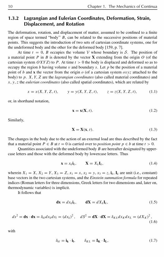
1.3.2 Lagrangian and Eulerian Coordinates, Deformation, Strain,Displacement, and Rotation
The deformation, rotation, and displacement of matter, assumed to be confined to a finiteregion of space termed “body’’ B, can be related to the successive positions of materialpoints. This suggests the introduction of two sets of cartesian coordinate systems, one forthe undeformed body and the other for the deformed body [159, p. 7].
At time t = 0, B occupies the volume V whose boundary is S. The position ofa material point P in B is denoted by the vector X extending from the origin O (of thecartesian system OXYZ) to P . At time t > 0 the body is displaced and deformed so as tooccupy the region b having volume v and boundary s. Let p be the position of a materialpoint of b and x the vector from the origin o (of a cartesian system oxyz attached to thebody) to p. X, Y,Z are the lagrangian coordinates (also called material coordinates) andx, y, z the eulerian coordinates (also called spatial coordinates), which are related by
x = x(X, Y,Z, t), y = y(X, Y,Z, t), z = z(X, Y, Z, t), (1.1)
or, in shorthand notation,
x = x(X, t). (1.2)
Similarly,
X = X(x, t). (1.3)
The changes in the body due to the action of an external load are thus described by the factthat a material point P ∈ B at t = 0 is carried over to position point p ∈ b at time t > 0.
Quantities associated with the undeformed body B are hereafter designated by upper-case letters and those with the deformed body by lowercase letters. Thus
x = xkik, X = XkIk, (1.4)
wherein X1 = X, X2 = Y , X3 = Z, x1 = x, x2 = y, x3 = z, ik , Ik are unit (i.e., constant)base vectors in the two cartesian systems, and the Einstein summation formula for repeatedindices (Roman letters for three dimensions, Greek letters for two dimensions and, later on,thermodynamic variables) is implicit.
It follows that
dx = dxkik, dX = dXkIk, (1.5)
ds2 = dx · dx = δkldxkdxl = (dxk)2 , dS2 = dX · dX = δKLdxKdxL = (dXK)
2 ,
(1.6)
with
δkl = ik · il, δKL = IK · IL, (1.7)
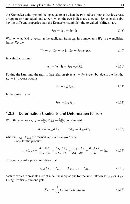
1.3. Underlying Principles of the Mechanics of Continua 11
the Kronecker delta symbols being equal to one when the two indices (both either lowercaseor uppercase) are equal, and to zero when the two indices are unequal. By extension (buthaving different properties than the Kronecker symbols), the so-called “shifters’’ are
δKk = δkK = IK · ik. (1.8)
With w = wk(x)ik a vector in the euclidean frame xk , its components WK in the euclideanframe XK are
WK = w · IK = wkik · IK = δKkwk(x). (1.9)
In a similar manner,
wk = W · ik = δKkWK(X). (1.10)
Putting the latter into the next-to-last relation gives wk = δKkδKlwl , but due to the fact thatwk = δklwl , one obtains
δkl = δKkδKl. (1.11)
In the same manner,
δKL = δKkδLk. (1.12)
1.3.3 Deformation Gradients and Deformation Tensors
With the notations xk,K ≡ ∂xk∂XK
, XK,k ≡ ∂XK∂xk
, one can write
dxk = xk,KdXK, dXK = XK,kdxk, (1.13)
wherein xk,K , XK,k are termed deformation gradients.Consider the product
xk,KXK,l = ∂xk
∂X1
∂X1
∂xl+ ∂xk
∂X2
∂X2
∂xl+ ∂xk
∂X3
∂X3
∂xl= ∂xk(X)
∂xl= δkl . (1.14)
This and a similar procedure show that
xk,KXK,l = δkl, XK,kxk,L = δKL, (1.15)
each of which represents a set of nine linear equations for the nine unknowns xk,K or XK,k .Using Cramer’s rule one gets
XK,k = 1
2JεKLMεklmxl,Lxm,M, (1.16)
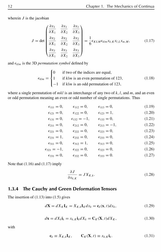
12 Chapter 1. The Mechanics of Continua
wherein J is the jacobian
J = det
∂x1
∂X1
∂x1
∂X2
∂x1
∂X3
∂x2
∂X1
∂x2
∂X2
∂x2
∂X3
∂x3
∂X1
∂x3
∂X2
∂x3
∂X3
= 1
6εKLMεklmxk,Kxl,Lxm,M, (1.17)
and εklm is the 3D permutation symbol defined by
εklm =
0 if two of the indices are equal,
1 if klm is an even permutation of 123,
−1 if klm is an odd permutation of 123,
(1.18)
where a single permutation of mkl is an interchange of any two of k, l, and m, and an evenor odd permutation meaning an even or odd number of single permutations. Thus
ε111 = 0, ε112 = 0, ε113 = 0, (1.19)
ε121 = 0, ε122 = 0, ε123 = 1, (1.20)
ε131 = 0, ε132 = −1, ε133 = 0, (1.21)
ε211 = 0, ε212 = 0, ε213 = −1, (1.22)
ε221 = 0, ε222 = 0, ε223 = 0, (1.23)
ε231 = 1, ε232 = 0, ε233 = 0, (1.24)
ε311 = 0, ε312 = 1, ε313 = 0, (1.25)
ε321 = −1, ε322 = 0, ε323 = 0, (1.26)
ε331 = 0, ε332 = 0, ε333 = 0. (1.27)
Note that (1.16) and (1.17) imply
∂J
∂xk,K= JXK,k. (1.28)
1.3.4 The Cauchy and Green Deformation Tensors
The insertion of (1.13) into (1.5) gives
dX = dXKIK = XK,kIKdxk = ck(x, t)dxk, (1.29)
dx = dXkik = xk,K ikdXk = CK(X, t)dXK, (1.30)
with
ck ≡ XK,kIK, CK(X, t) ≡ xk,K ik. (1.31)

1.3. Underlying Principles of the Mechanics of Continua 13
One can express I and i in terms of c and C by employing (1.15):
IK = xk,Kck, ik = XK,kCK. (1.32)
Employing (1.29) and (1.31) in (1.6) leads to
ds2 = ckldxkdxl, dS2 = CKLdXKdXL, (1.33)
wherein
ckl(x, t) ≡ ck · cl = XK,kXK,l, (1.34)
is the Cauchy deformation tensor and
CKL(X, t) ≡ CK · CL = xk,Kxk,L, (1.35)
Green’s deformation tensor. Both are symmetric and positive definite.
1.3.5 Strain Tensors and Displacement Vectors
The difference ds2 − dS2, for the same material points in B and b, is a measure of thechange of length so that vanishing ds2 − dS2 denotes a situation in which deformation hasnot changed the distance between two neighboring points. If this is so for all points in thebody, the body is subject only to a rigid displacement. This difference can be written ineither of the two euclidian frames as
ds2 − dS2 = (CKL − δKL)dXKdXL = 2EKL(X, t)dXKdXL, (1.36)
ds2 − dS2 = (δkl − ckl)dxkdxl = 2ekl(x, t)dxkdxl, (1.37)
wherein
2EKL ≡ CKL(X, t)− δKL (1.38)
is the lagrangian strain tensor and
2ekl ≡ δkl − ckl(x, t) (1.39)
the eulerian strain tensor.When either of these strain tensors vanishes, one obtains, via (1.36) and (1.37),
EKLdXKdXL = ekldxkdxl , so that
EKL = ekl∂xk
∂XK
∂xl
∂XL= eklxk,Kxl,L, (1.40)
ekl = EKL∂XK
∂xk
∂XL
∂xl= EKLXK,kXL,l . (1.41)
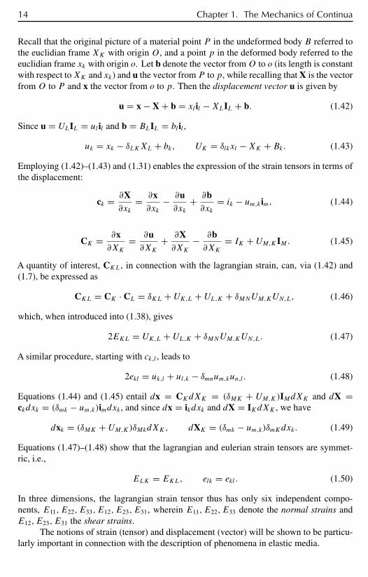
14 Chapter 1. The Mechanics of Continua
Recall that the original picture of a material point P in the undeformed body B referred tothe euclidian frame XK with origin O, and a point p in the deformed body referred to theeuclidian frame xk with origin o. Let b denote the vector fromO to o (its length is constantwith respect toXK and xk) and u the vector from P to p, while recalling that X is the vectorfrom O to P and x the vector from o to p. Then the displacement vector u is given by
u = x − X + b = xl il −XLIL + b. (1.42)
Since u = ULIL = ul il and b = BLIL = bl il ,
uk = xk − δLKXL + bk, UK = δlkxl −XK + Bk. (1.43)
Employing (1.42)–(1.43) and (1.31) enables the expression of the strain tensors in terms ofthe displacement:
ck = ∂X∂xk
= ∂x∂xk
− ∂u∂xk
+ ∂b∂xk
= ik − um,kim, (1.44)
CK = ∂x∂XK
= ∂u∂XK
+ ∂X∂XK
− ∂b∂XK
= IK + UM,KIM. (1.45)
A quantity of interest, CKL, in connection with the lagrangian strain, can, via (1.42) and(1.7), be expressed as
CKL = CK · CL = δKL + UK,L + UL,K + δMNUM,KUN,L, (1.46)
which, when introduced into (1.38), gives
2EKL = UK,L + UL,K + δMNUM,KUN,L. (1.47)
A similar procedure, starting with ck,l , leads to
2ekl = uk,l + ul,k − δmnum,kun,l . (1.48)
Equations (1.44) and (1.45) entail dx = CKdXK = (δMK + UM,K)IMdXK and dX =ckdxk = (δmk − um,k)imdxk , and since dx = ikdxk and dX = IKdXK , we have
dxk = (δMK + UM,K)δMkdXK, dXK = (δmk − um,k)δmKdxk. (1.49)
Equations (1.47)–(1.48) show that the lagrangian and eulerian strain tensors are symmet-ric, i.e.,
ELK = EKL, elk = ekl . (1.50)
In three dimensions, the lagrangian strain tensor thus has only six independent compo-nents, E11, E22, E33, E12, E23, E31, wherein E11, E22, E33 denote the normal strains andE12, E23, E31 the shear strains.
The notions of strain (tensor) and displacement (vector) will be shown to be particu-larly important in connection with the description of phenomena in elastic media.
1.3. Underlying Principles of the Mechanics of Continua 15
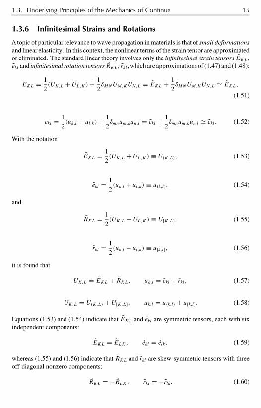
1.3.6 Infinitesimal Strains and Rotations
Atopic of particular relevance to wave propagation in materials is that of small deformationsand linear elasticity. In this context, the nonlinear terms of the strain tensor are approximatedor eliminated. The standard linear theory involves only the infinitesimal strain tensors EKL,ekl and infinitesimal rotation tensors RKL, rkl , which are approximations of (1.47) and (1.48):
EKL = 1
2(UK,L + UL,K)+ 1
2δMNUM,KUN,L = EKL + 1
2δMNUM,KUN,L EKL,
(1.51)
ekl = 1
2(uk,l + ul,k)+ 1
2δmnum,kun,l = ekl + 1
2δmnum,kun,l ekl . (1.52)
With the notation
EKL = 1
2(UK,L + UL,K) ≡ U(K,L), (1.53)
ekl = 1
2(uk,l + ul,k) ≡ u(k,l), (1.54)
and
RKL = 1
2(UK,L − UL,K) ≡ U[K,L], (1.55)
rkl = 1
2(uk,l − ul,k) ≡ u[k,l], (1.56)
it is found that
UK,L = EKL + RKL, uk,l = ekl + rkl , (1.57)
UK,L = U(K,L) + U[K,L], uk,l = u(k,l) + u[k,l]. (1.58)
Equations (1.53) and (1.54) indicate that EKL and ekl are symmetric tensors, each with sixindependent components:
EKL = ELK, ekl = elk, (1.59)
whereas (1.55) and (1.56) indicate that RKL and rkl are skew-symmetric tensors with threeoff-diagonal nonzero components:
RKL = −RLK, rkl = −rlk. (1.60)
16 Chapter 1. The Mechanics of Continua
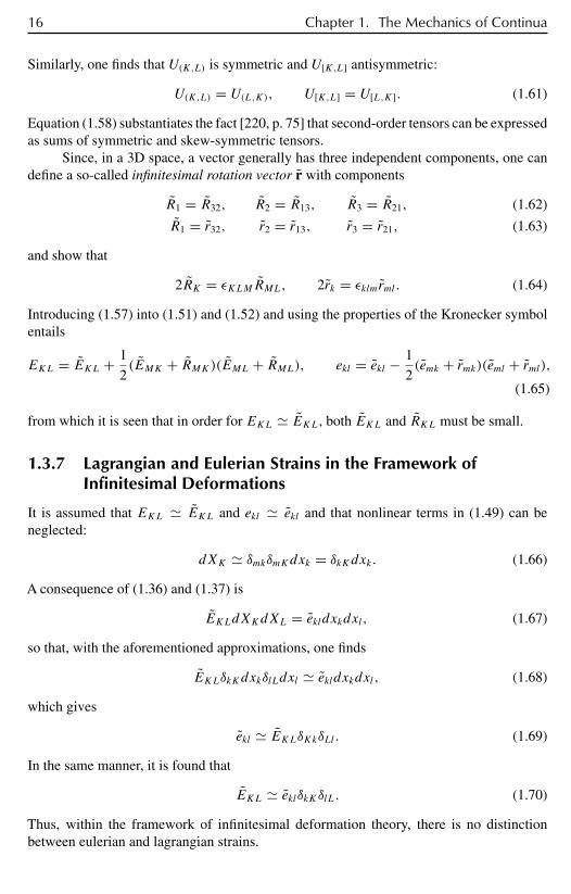
Similarly, one finds that U(K,L) is symmetric and U[K,L] antisymmetric:
U(K,L) = U(L,K), U[K,L] = U[L,K]. (1.61)
Equation (1.58) substantiates the fact [220, p. 75] that second-order tensors can be expressedas sums of symmetric and skew-symmetric tensors.
Since, in a 3D space, a vector generally has three independent components, one candefine a so-called infinitesimal rotation vector r with components
R1 = R32, R2 = R13, R3 = R21, (1.62)
R1 = r32, r2 = r13, r3 = r21, (1.63)
and show that
2RK = εKLMRML, 2rk = εklmrml. (1.64)
Introducing (1.57) into (1.51) and (1.52) and using the properties of the Kronecker symbolentails
EKL = EKL + 1
2(EMK + RMK)(EML + RML), ekl = ekl − 1
2(emk + rmk)(eml + rml),
(1.65)
from which it is seen that in order for EKL EKL, both EKL and RKL must be small.
1.3.7 Lagrangian and Eulerian Strains in the Framework ofInfinitesimal Deformations
It is assumed that EKL EKL and ekl ekl and that nonlinear terms in (1.49) can beneglected:
dXK δmkδmKdxk = δkKdxk. (1.66)
A consequence of (1.36) and (1.37) is
EKLdXKdXL = ekldxkdxl, (1.67)
so that, with the aforementioned approximations, one finds
EKLδkKdxkδlLdxl ekldxkdxl, (1.68)
which gives
ekl EKLδKkδLl. (1.69)
In the same manner, it is found that
EKL eklδkKδlL. (1.70)
Thus, within the framework of infinitesimal deformation theory, there is no distinctionbetween eulerian and lagrangian strains.

1.3. Underlying Principles of the Mechanics of Continua 17
1.3.8 Strain Invariants and Principal Directions
In [159, pp. 28–31], it was shown how the deformations in a body transform an infinitesimalsphere therein into an ellipsoid, called the strain ellipsoid. Deformation also rotates theprincipal directions of the ellipsoid. The strain components, referred to the principal axesof the strain ellipsoid, can be expressed in terms of those referred to any other axes oncethe cosine directors of the principal directions are found.
An important task is to find the principal directions and primitive functions of strainsthat are invariant during such coordinate transformations. The so-called principal strainsare solutions E of the equation
det
E11 − E E12 E13
E21 E22 − E E23
E31 E32 E33 − E
= 0. (1.71)
This leads to the cubic equation
E3 + IEE2 − IIEE + IIIE = 0, (1.72)
wherein
IE = EKK = E11 + E22 + E33, (1.73)
IIE = det
(E22 E23
E32 E33
)+ det
(E11 E31
E13 E33
)+ det
(E11 E12
E21 E22
), (1.74)
IIIE = det
E11 E12 E13
E21 E22 E23
E31 E32 E33
. (1.75)
The characteristic equation (1.72) possesses the three roots E1, E2, E3, which are termedprincipal strains. Then the coefficients IE, IIE, IIIE can be expressed in terms of theseprincipal strains:
IE = E1 + E2 + E3,
I IE = E2E3 + E3E1 + E1E2,
I IIE = E1E2E3.
(1.76)
Thus, IE, IIE, IIIE are invariant with respect to any coordinate transformation at P .This result substantiates the fact that in three dimensions, there exist no more than threeindependent invariants of a second-order tensor.
Invariants may also be obtained via (1.38), (1.39) in terms of the strain tensors EKL,ekl , ekl , CKL, ckl . For instance,
IC = 3 + 2IE, Ic = 3 − 2Ie,I IC = 3 + 4IE + 4IIE, IIc = 3 − 4Ie + 4IIe,
I IIC = 1 + 2IE + 4IIE + 8IIIE, IIIc = 1 − 2Ie + 4IIe − 8IIIe.(1.77)
with
Ic = IIC
IIIC, IIc = IC
IIIC, IIIc = 1
IIIC. (1.78)

18 Chapter 1. The Mechanics of Continua
1.3.9 Area and Volume Changes Due to Infinitesimal Deformations
An infinitesimal parallelepiped within the body, with edge vectors I1dX1, I2dX2, I3dX3, istransformed, subsequent to deformation, into a rectilinear parallelepiped with edge vectorsC1dX1, C2dX2, C3dX3, where (see (1.45))
CK = xk,K ik. (1.79)
One of the three area vectors is
da3 = (C1dX1)× (C2dX2) = xk,1xl,2dX1dX2ik × il , (1.80)
which, on account of dA3 = dX1dX2 and
ik × il = εklmim, (1.81)
becomes
da3 = εklmxk,1xl,2imdA3. (1.82)
With the definition (1.17), (1.19) of the jacobian,
J = 1
6εKLMεklmxk,Kxl,Lxm,M = εklmxk,1xl,2xm,3, (1.83)
one finds, with the help of (1.15),
JX3,m = εklmxk,1xl,2xm,3X3,m = εklmxk,1xl,2, (1.84)
which, upon introduction into (1.82), yields
da3 = JX3,mimdA3. (1.85)
More generally,
dal = JXl,mimdAl, (1.86)
so that
da = da1 + da2 + da3 = JXK,kdAK ik = dakik. (1.87)
Recalling (1.35), one finds, with the help of (1.17),
det(CKL) = det(xk,K)det(xk,L) = J 2. (1.88)
In the same way that (1.75) was obtained, one can show that
IIIC = det(CKL), (1.89)
1.3. Underlying Principles of the Mechanics of Continua 19
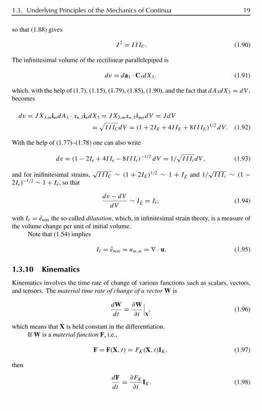
so that (1.88) gives
J 2 = IIIC. (1.90)
The infinitesimal volume of the rectilinear parallelepiped is
dv = da3 · C3dX3, (1.91)
which, with the help of (1.7), (1.15), (1.79), (1.85), (1.90), and the fact that dA3dX3 = dV ,becomes
dv = JX3,mimdA3 · xn,3indX3 = JX3,mxn,3δmndV = JdV
= √IIICdV = (1 + 2IE + 4IIE + 8IIIE)
1/2 dV . (1.92)
With the help of (1.77)–(1.78) one can also write
dv = (1 − 2Ie + 4IIe − 8IIIe)−1/2 dV = 1/
√IIIcdV, (1.93)
and for inifinitesimal strains,√IIIC ∼ (1 + 2IE)1/2 ∼ 1 + IE and 1/
√IIIc ∼ (1 −
2Ie)−1/2 ∼ 1 + Ie, so that
dv − dVdV
∼ IE = Ie, (1.94)
with Ie = emm the so-called dilatation, which, in infinitesimal strain theory, is a measure ofthe volume change per unit of initial volume.
Note that (1.54) implies
Ie = emm = um,m = ∇ · u. (1.95)
1.3.10 Kinematics
Kinematics involves the time rate of change of various functions such as scalars, vectors,and tensors. The material time rate of change of a vector W is
dWdt
= ∂W∂t
∣∣∣X, (1.96)
which means that X is held constant in the differentiation.If W is a material function F, i.e.,
F = F(X, t) = FK(X, t)IK, (1.97)
then
dFdt
= ∂FK
∂tIK. (1.98)
20 Chapter 1. The Mechanics of Continua
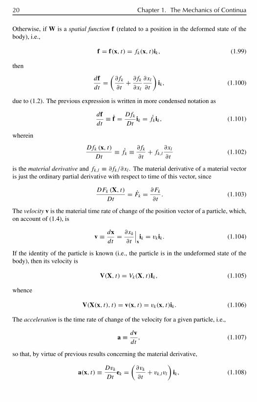
Otherwise, if W is a spatial function f (related to a position in the deformed state of thebody), i.e.,
f = f(x, t) = fk(x, t)ik, (1.99)
then
dfdt
=(∂fk
∂t+ ∂fk
∂xl
∂xl
∂t
)ik, (1.100)
due to (1.2). The previous expression is written in more condensed notation as
dfdt
≡ f = Dfk
Dtik = fkik, (1.101)
wherein
Dfk (x, t)Dt
≡ fk ≡ ∂fk
∂t+ fk,l ∂xl
∂t(1.102)
is the material derivative and fk,l ≡ ∂fk/∂xl . The material derivative of a material vectoris just the ordinary partial derivative with respect to time of this vector, since
DFk (X, t)Dt
= Fk = ∂Fk
∂t. (1.103)
The velocity v is the material time rate of change of the position vector of a particle, which,on account of (1.4), is
v ≡ dxdt
= ∂xk
∂t
∣∣∣xik = vkik. (1.104)
If the identity of the particle is known (i.e., the particle is in the undeformed state of thebody), then its velocity is
V(X, t) = Vk(X, t)Ik, (1.105)
whence
V(X(x, t), t) = v(x, t) = vk(x, t)ik. (1.106)
The acceleration is the time rate of change of the velocity for a given particle, i.e.,
a ≡ dvdt, (1.107)
so that, by virtue of previous results concerning the material derivative,
a(x, t) ≡ Dvk
Dtek =
(∂vk
∂t+ vk,lvl
)ik, (1.108)

1.3. Underlying Principles of the Mechanics of Continua 21
whereas in lagrangian coordinates,
a(X, t) ≡ ∂Vk (X, t)∂t
∣∣∣x. (1.109)
In the lagrangian representation, the particle with a given velocity or acceleration is known,as in the (classical) mechanics of the particle. In the eulerian representation, the velocityand acceleration at time t and spatial point x are known, but the particle occupying thispoint at this time is not known (it could be any of the material particles of the undeformedbody).
The material derivative of elements of arc, surface, and volume intervene in variousbalance and conservation laws. In [159, pp. 70–73], it is shown that (i)
D
Dt(dxk) = vk,ldxl (1.110)
with dxk ≡ xk,ldXl ; (ii) the material derivative of a cartesian component of an element ofarea da is
D
Dt(dak) = vm,mdak − vm,kdam; (1.111)
and (iii) the material derivative of the volume element dv is
D
Dt(dv) = vk,kdv. (1.112)
1.3.11 Material Derivatives of Line, Surface, and Volume Integralsover Regions Devoid of Discontinuities
The material derivative of a line integral of a scalar field φ over a material line C is
IC = D
Dt
∫Cφdxk. (1.113)
A material line C can be described by the equation X = X(S), with S arc length so that nodifferentiation of C is necessary. This means that
IC =∫
C
D
Dt(φdxk) =
∫Cdxk
Dφ
Dt+∫
CφD
Dt(dxk), (1.114)
which, on account of (1.110), yields
IC = D
Dt
∫Cφdxk =
∫C(φdxk + φvk,ldxl). (1.115)
The time rate of change of a line integral over a spatially fixed line c is
Ic = ∂
∂t
∫c
φdxk =∫c
∂φ
∂tdxk, (1.116)
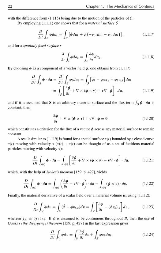
22 Chapter 1. The Mechanics of Continua
with the difference from (1.115) being due to the motion of the particles of C.By employing (1.111) one shows that for a material surface S
D
Dt
∫Sφdak =
∫S
[φdak + φ (−vl,kdal + vl,ldak)] , (1.117)
and for a spatially fixed surface s
∂
∂t
∫s
φdak =∫s
∂φ
∂tdak. (1.118)
By choosing φ as a component of a vector field φ, one obtains from (1.117)
D
Dt
∫Sφ · da = D
Dt
∫Sφkdak =
∫S
[φk − φlvk,l + φkvl,l
]dak
=∫
S
[∂φ
∂t+ ∇ × (φ × v)+ v∇ · φ
]· da, (1.119)
and if it is assumed that S is an arbitrary material surface and the flux term∫S φ · da is
constant, then
∂φ
∂t+ ∇ × (φ × v)+ v∇ · φ = 0, (1.120)
which constitutes a criterion for the flux of a vector φ across any material surface to remainconstant.
A result similar to (1.119) is found for a spatial surface s(t) bounded by a closed curvec(t) moving with velocity ν (s(t) + c(t) can be thought of as a set of fictitious materialparticles moving with velocity ν):
D
Dt
∫s(t)
φ · da =∫s(t)
[∂φ
∂t+ ∇ × (φ × ν)+ ν∇ · φ
]· da, (1.121)
which, with the help of Stokes’s theorem [159, p. 427], yields
D
Dt
∫s(t)
φ · da =∫s(t)
(∂φ
∂t+ ν∇ · φ
)· da +
∫c(t)
(φ × ν) · dc. (1.122)
Finally, the material derivative of a scalar field over a material volume is, using (1.112),
D
Dt
∫Vφdv =
∫V(φ + φvk,k)dv =
∫V
[∂φ
∂t+ (φvk),k
]dv, (1.123)
wherein f,k ≡ ∂f/∂xk . If φ is assumed to be continuous throughout B, then the use ofGauss’s (the divergence) theorem [159, p. 427] in the last expression gives
D
Dt
∫Vφdv =
∫V
∂φ
∂tdv +
∫Sφvkdak. (1.124)

1.3. Underlying Principles of the Mechanics of Continua 23
A remarkable result (due to the formal similarity with (1.124)) is that when V and S arereplaced instantaneously with a fixed spatial volume v and boundary s, then
D
Dt
∫Vφdv =
∫v
∂φ
∂tdv +
∫s
φvkdak, (1.125)
which signifies that the rate of change of a scalar field φ over a material volume V is equalto the sum of the rate of creation of φ in a fixed volume v instantaneously coinciding withV and the flux φvk through the boundary surface s of v.
Another remarkable result (again due to the formal similarity with (1.124), for anarbitrary spatial volume v(t) bounded by the closed surface s(t) and moving with thevelocity ν) is that
D
Dt
∫v(t)
φdv =∫v(t)
∂φ
∂tdv +
∫s
φν · da. (1.126)
1.3.12 Material Derivatives of Integrals over Regions Containing aDiscontinuity Surface
First consider the situation in which a discontinuity surface σ(t), moving with velocity ν,cuts through the material volume V [159, p. 76]. This discontinuity surface divides V intotwo uniform portions V+ and V− bounded by S+ + σ+ and S− + σ−, respectively, so thatapplying (1.126) in each of these regions leads to
D
Dt
∫V±φdv =
∫V±
∂φ
∂tdv +
∫S±φν · da ∓
∫σ±φν · da, (1.127)
which, when added and after taking the limit σ± → σ , give
D
Dt
∫V−σ
φdv =∫
V−σ∂φ
∂tdv +
∫S−σ
φν · da −∫σ
[[φν]] · da, (1.128)
wherein [[A]] ≡ A+ − A−. Using the Gauss theorem, the last expression takes the form
D
Dt
∫V−σ
φdv =∫
V−σ
[∂φ
∂t+ ∇ · (φν)
]dv +
∫σ
[[φ(v − ν)]] · da. (1.129)
Asimilar procedure can be applied [159, p. 77] to a material surface S bounded by the closedcurve C on which a discontinuity line γ (t) is moving with velocity ν. At a given instant t ,this line divides S into two portions S+ and S−. Assuming that the normal component ofν to γ is continuous, one finds, from (1.119) and with the help of the Stokes theorem,
D
Dt
∫Sφ · da =
∫S−γ
[∂φ
∂t+ ∇ × (φ × v)+ v∇ · φ
]· da
+∫γ
[[φ × (v − ν)]] · kds, (1.130)
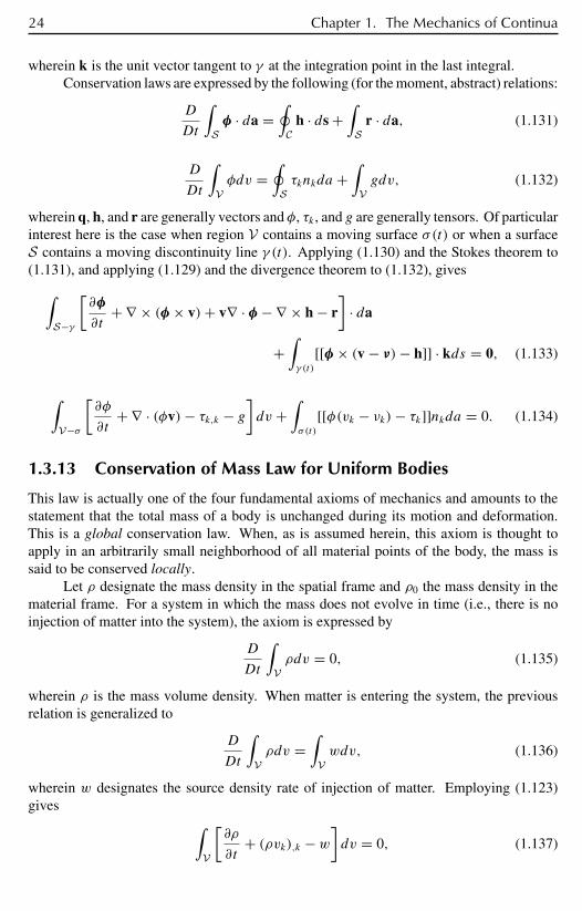
24 Chapter 1. The Mechanics of Continua
wherein k is the unit vector tangent to γ at the integration point in the last integral.Conservation laws are expressed by the following (for the moment, abstract) relations:
D
Dt
∫Sφ · da =
∮C
h · ds +∫
Sr · da, (1.131)
D
Dt
∫Vφdv =
∮Sτknkda +
∫Vgdv, (1.132)
wherein q, h, and r are generally vectors and φ, τk , and g are generally tensors. Of particularinterest here is the case when region V contains a moving surface σ(t) or when a surfaceS contains a moving discontinuity line γ (t). Applying (1.130) and the Stokes theorem to(1.131), and applying (1.129) and the divergence theorem to (1.132), gives∫
S−γ
[∂φ
∂t+ ∇ × (φ × v)+ v∇ · φ − ∇ × h − r
]· da
+∫γ (t)
[[φ × (v − ν)− h]] · kds = 0, (1.133)
∫V−σ
[∂φ
∂t+ ∇ · (φv)− τk,k − g
]dv +
∫σ(t)
[[φ(vk − νk)− τk]]nkda = 0. (1.134)
1.3.13 Conservation of Mass Law for Uniform Bodies
This law is actually one of the four fundamental axioms of mechanics and amounts to thestatement that the total mass of a body is unchanged during its motion and deformation.This is a global conservation law. When, as is assumed herein, this axiom is thought toapply in an arbitrarily small neighborhood of all material points of the body, the mass issaid to be conserved locally.
Let ρ designate the mass density in the spatial frame and ρ0 the mass density in thematerial frame. For a system in which the mass does not evolve in time (i.e., there is noinjection of matter into the system), the axiom is expressed by
D
Dt
∫Vρdv = 0, (1.135)
wherein ρ is the mass volume density. When matter is entering the system, the previousrelation is generalized to
D
Dt
∫Vρdv =
∫Vwdv, (1.136)
wherein w designates the source density rate of injection of matter. Employing (1.123)gives ∫
V
[∂ρ
∂t+ (ρvk),k − w
]dv = 0, (1.137)

1.3. Underlying Principles of the Mechanics of Continua 25
and since this global form of the law of conservation of mass holds for arbitrary V , onededuces from it the local form of the conservation of mass law
∂ρ
∂t+ (ρvk),k = w. (1.138)
Although this expression is suitable for fluids, it turns out that another relation is moresuitable for solids and is given by ∫
Vρdv =
∫V
ρ0dV, (1.139)
or, on account of (1.92), ∫V
(ρ0 − ρJ )dV = 0. (1.140)
For this to be valid for every volume element, one must have (see also (1.92) and (1.77))
ρ0 = ρJ = ρ√IIIC = ρ
√1 + 2IE + 4IIE + 8IIIE, (1.141)
which is the local form of the conservation of mass law, equivalent to (1.138).
1.3.14 Conservation of Momentum and Energy Laws
These laws are actually the expression of three axioms. The first, deriving from Newton’ssecond law, takes the form
D
Dt
∫Vρvkdv = Fk, (1.142)
wherein Fk is the kth cartesian component of the resultant force F acting on the body. Amore detailed global form of this law is given later on from which will be derived a localform of the conservation of momentum law. Before doing this it is necessary to distinguishbetween external and internal forces (i.e., loads) and then introduce the notion of stress.
Another equation translates the axiom of conservation of momentum, and yet anotherrelation expresses the conservation of energy [159, pp. 84–86].
1.3.15 External and Internal Loads and Their Incorporation in theConservation of Momentum Equation
Bodies of matter are deformed and displaced under the influence of external forces. How-ever, deformation is also caused by the action of internal forces. These forces have to becategorized in order to relate them to their effects.
An almost trivial statement is that the resultant of forces acting on a body is
F =∫
VdF. (1.143)

26 Chapter 1. The Mechanics of Continua
Insofar as the resultant of internal forces (due to the action of one particle on another) is nil(according to Newton’s third law of action and reaction), F in the preceding equation canbe considered an external, and therefore usually known, force. This force is due either toextrinsic body (or volume) loads such as gravity or to extrinsic surface (or contact) loadsthat arise from the action of one body on another across their boundaries.
The extrinsic surface force per unit area is called the surface traction, an example ofwhich is the hydrostatic pressure exerted by a fluid acting on a submerged body. If f denotesthe body force per unit mass and t(n) the surface traction per unit area acting on the surfaceof the body with exterior unit normal n, then
F =∮
St(n)da +
∫Vρfdv, (1.144)
where the body force and surface force densities can eventually be considered distributionsto account for concentrated forces acting at isolated points. Consequently, the conservationof momentum (Euler) equation (1.142) takes the general form
D
Dt
∫Vρvdv =
∮S
t(n)da +∫
Vρfdv. (1.145)
1.3.16 Stress
Consider a small closed subregion, of volume v and boundary s, fully contained in the bodyof volume V and boundary S. At a point p ∈ s, V − v makes itself felt by (i) surface forcest(n) called stress vectors, (ii) surface couples termed couple stress vectors, (iii) body forceswhose density is designated by ρf , and (iv) body couples. The surface loads vary with theposition p ∈ s and with the exterior unit normal vector at p. The law of conservation ofmomentum, expressed by (1.145), which was previously applied to the body V + S, holdsalso for the subbody v + s by replacing the domains of integration V and S by v and s,respectively.
In [159, pp. 97–98], it is shown, by applying this conservation of momentum law andthe conservation of mass law to a small tetrahedron-shaped subbody, that the stress vectort(n) at a point p ∈ s is a known linear function of the stress vectors tk acting on the coordinatesurfaces passing through this point, i.e.,
t(n) = tknk. (1.146)
To render the notion of stress objective, i.e., independent of the coordinate frame, oneintroduces the stress tensor tkl related to tk by
tk = tkl il , (1.147)
where, as before, the il are unit vectors along the coordinate axes. The first subscript intkl indicates the coordinate surface xk = const. on which the stress vector tk acts, and thesecond indicates the direction of the component of tk so that t11, t22, t33 are normal stressesand the other components of tkl are shear stresses. The units of both normal and shearstress are force per unit area. Note that the stress tensor is often designated by the symbolσkl or τkl .
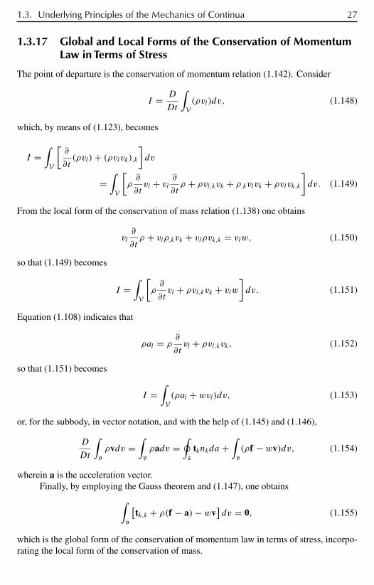
1.3. Underlying Principles of the Mechanics of Continua 27
1.3.17 Global and Local Forms of the Conservation of MomentumLaw in Terms of Stress
The point of departure is the conservation of momentum relation (1.142). Consider
I = D
Dt
∫V(ρvl)dv, (1.148)
which, by means of (1.123), becomes
I =∫
V
[∂
∂t(ρvl)+ (ρvlvk),k
]dv
=∫
V
[ρ∂
∂tvl + vl ∂
∂tρ + ρvl,kvk + ρ,kvlvk + ρvlvk,k
]dv. (1.149)
From the local form of the conservation of mass relation (1.138) one obtains
vl∂
∂tρ + vlρ,kvk + vlρvk,k = vlw, (1.150)
so that (1.149) becomes
I =∫
V
[ρ∂
∂tvl + ρvl,kvk + vlw
]dv. (1.151)
Equation (1.108) indicates that
ρal = ρ∂
∂tvl + ρvl,kvk, (1.152)
so that (1.151) becomes
I =∫
V(ρal + wvl)dv, (1.153)
or, for the subbody, in vector notation, and with the help of (1.145) and (1.146),
D
Dt
∫v
ρvdv =∫
v
ρadv =∮
s
tknkda +∫
v
(ρf − wv)dv, (1.154)
wherein a is the acceleration vector.Finally, by employing the Gauss theorem and (1.147), one obtains∫
v
[tk,k + ρ(f − a)− wv
]dv = 0, (1.155)
which is the global form of the conservation of momentum law in terms of stress, incorpo-rating the local form of the conservation of mass.

28 Chapter 1. The Mechanics of Continua
For this law to be valid for an arbitrary volume v, one must have
tk,k + ρ(f − a)− wv = 0, (1.156)
or, after use of (1.147),
tlk,k + ρ(fk − ak)− wvk = 0, (1.157)
which is the local form of the conservation of momentum law. By a similar procedure, basedon an analysis of the conservation of the moment of momentum, it can be shown that, for alarge class of (nonpolar) materials, the stress tensor is symmetric, i.e.,
tlk = tkl . (1.158)
The last two equations are Cauchy’s first and second laws of motion.
1.3.18 Local Form of the Boundary Conditions on DiscontinuitySurfaces
The starting point is (1.131)–(1.134). Taking φ = ρ therein gives, on account of (1.137)(i.e., this amounts to taking g = w and τk = 0),∫
V−σ
[∂ρ
∂t+ ∇ · (ρv)− w
]dv +
∫σ
[[ρ(vk − νk)]]nkda = 0. (1.159)
Using (1.138) yields ∫σ
[[ρ(vk − νk)]]nkda = 0, (1.160)
which, for arbitrary σ , implies
[[ρ(vk − νk)]]nkda = 0. (1.161)
Considering the definition of ν (it is the velocity of the moving surface σ and therefore notdiscontinuous), the last expression can be written as
[[ρv]] · n − [[ρ]]ν · n = 0, (1.162)
this being the local form of the boundary condition resulting from the continuity of massrelation.
The choices φ = ρvl , τk = tk , and g = ρfl − wvl in (1.134) give∫V−σ
[∂(ρvl)
∂t+ ∇ · (ρvlv)− tk,k − ρfl + wvl
]dv +
∫σ
[[ρvl(vk − νk)− tk]]nkda = 0.
(1.163)
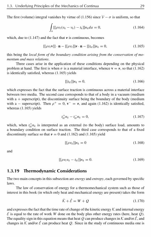
1.3. Underlying Principles of the Mechanics of Continua 29
The first (volume) integral vanishes by virtue of (1.156) since V − σ is uniform, so that∫σ
[[ρvl(vk − νk)− tk]]nkda = 0, (1.164)
which, due to (1.147) and the fact that ν is continuous, becomes
[[ρvlv]] · n − [[ρvl]]ν · n − [[tkl]]nk = 0, (1.165)
this being the local form of the boundary condition arising from the conservation of mo-mentum and mass relations.
Three cases arise in the application of these conditions depending on the physicalproblem at hand. The first is when σ is a material interface, whence v = ν, so that (1.162)is identically satisfied, whereas (1.165) yields
[[tkl]]nk = 0, (1.166)
which expresses the fact that the surface traction is continuous across a material interfacebetween two media. The second case corresponds to that of a body in a vacuum (mediumwith a + superscript), the discontinuity surface being the boundary of the body (mediumwith a − superscript). Then ρ+ = 0, v− = ν, and again (1.162) is identically satisfied,whereas (1.165) yields
t+kl nk − t−kl nk = 0, (1.167)
which, when t+kl nk is interpreted as an external (to the body) surface load, amounts toa boundary condition on surface traction. The third case corresponds to that of a fixeddiscontinuity surface so that ν = 0 and (1.162) and (1.165) yield
[[ρvk]]nk = 0 (1.168)
and
[[ρvlvk − tkl]]nk = 0. (1.169)
1.3.19 Thermodynamic Considerations
The two main concepts in this subsection are energy and entropy, each governed by specificlaws.
The law of conservation of energy for a thermomechanical system such as those ofinterest in this book (in which only heat and mechanical energy are present) takes the form
K + E = W +Q (1.170)
and expresses the fact that the time rate of change of the kinetic energy K and internal energyE is equal to the rate of work W done on the body plus other energy rates (here, heat Q).The equality sign in this equation means that heatQ can produce changes in K and/or E , andchanges in K and/or E can produce heat Q. Since in the study of continuous media one is
30 Chapter 1. The Mechanics of Continua
primarily interested in body deformation, the point of view is primarily one of thermostatics,this meaning that the change of kinetic energy is considered negligible compared to theother thermodynamic quantities, i.e., K ≈ 0, which, with E ≡ dE ,Wdt ≡ δW ,Qdt ≡ δQ,enables one to obtain from (1.169)
dE = δW + δQ, (1.171)
which is an expression of the first law of thermodynamics. The units for Q and W in theabove expressions are force times distance per unit time.
In a uniform body V + S, heat can enter the body through S or be supplied fromwithin V via distributed heat sources per unit mass h. Let q denote the heat vector per unitarea acting at point x of S and directed outwards with respect to the body (whose outwardunit normal vector is n at point x). The total heat input is
Q =∮
Sq · nda +
∫Vρhdv, (1.172)
whereas, by definition,
K = 1
2
∫Vρvkvkdv, (1.173)
E =∫
Vρεdv, (1.174)
and ε is the internal energy density per unit mass of the body.The mechanical energy is the work done by surface and body forces per unit time:
W =∮
Stlkvknlda +
∫Vρfkvkdv. (1.175)
Taking the time derivatives of the kinetic and internal energies and employing the divergencetheorem in the expressions ofQ andW yields
K =∫
V
[ρvkakdv + 1
2vkvk
D
Dt(ρdv)
], (1.176)
E =∫
V
[ρεdv + ε D
Dt(ρdv)
], (1.177)
W =∫
V
[tlk,lvk + tlkvk,l + ρfkvk
]dv, (1.178)
Q =∫
V
[qk,d + ρh] dv, (1.179)
1.3. Underlying Principles of the Mechanics of Continua 31
which, when inserted into (1.170), gives the following expression of global conservationof energy: ∫
V
(ρε − tlkvk,l − qk,k − ρh) dv +
∫V
(ε + 1
2vkvk
)D
Dt(ρdv)
−∫
Vvk(tlk,l + ρfk − ρak
)dv = 0. (1.180)
Henceforth, it is assumed that no matter is injected into the body, so that the second integralin the last expression vanishes. Also, on account of the conservation of momentum law, thethird integral vanishes so that, for arbitrary V , one obtains the local form of the conservationof energy law:
ρε = tklvl,k + qk,k + ρh. (1.181)
Using the second Cauchy law of motion (1.158), and with
dkl = vk,l + vl,k2
= dlk, (1.182)
the deformation rate (symmetric) tensor, one can express the local form of conservation ofenergy as
ρε = tkldlk + qk,k + ρh. (1.183)
The concepts of entropy and temperature are considered to have a self-evident status anal-ogous to that of mass.
Let η designate the entropy density whose dimensions are energy per unit temperatureper unit mass. Let θ designate the temperature and recall that ε designates the internalenergy density. The set of n + 1 independent variables η, υ ≡ υα , α = 1, 2, . . . , n, onwhich depend ε and θ at a material point X corresponding to a position x at time t , defines thethermodynamic state of the body. The entries (υα) of υ have the dimensions of mechanicalentities. η is independent of υ so that
ε = ε(η,υ,X), (1.184)
θ = θ(η,υ,X), (1.185)
which are the so-called thermodynamic constitutive equations for internal energy and tem-perature.
The choice of υ is discussed in [159, p. 124]. The upshot is that υ cannot be time,position, velocity, etc., and hence the internal energy and entropy density are not explicitfunctions of x and t , but they are dependent on the values of η and υ at location x and time t .There is some evidence that for dilute gases and some fluids, one should consider υ1 = 1/ρand all other entries of υ to be irrelevant. The changes in ε and θ due to changes in υ andθ are collectively termed a thermodynamic process.

32 Chapter 1. The Mechanics of Continua
Many of the working principles of thermodynamics, like those of continuum me-chanics, derive from a series of axioms. The foremost of these is the Clausius–Duheminequality
≡ dH
dt− B −
∮S · da ≥ 0, (1.186)
wherein is the total entropy production,H the total entropy, S the entropy passing throughS, and B the entropy resulting from sources in the body, which, for a uniform body, aregiven by
H =∫
Vρηdv, (1.187)
B =∫
Vρbdv, (1.188)
and b is the local entropy source per unit mass.The surface integral in (1.186) can be transformed into a volume integral via the Gauss
theorem, enabling (for arbitrary V) the following relation, translating the local form of theproduction of entropy:
ργ ≡ ρη − ρb − ∇ · S ≥ 0, (1.189)
wherein γ designates the local entropy production. The particular form of this equationdepends on the type of process (thermal, diffusion, chemical, etc.). Whatever this type is,one can express S and b by
S = qθ
+ S1, (1.190)
b = h
θ+ b1, (1.191)
where q/θ is the entropy influx due to heat input, h/θ is the entropy source supplied by theenergy source, and the remaining terms are due to other effects. Combining (1.191) and thelocal form of the conservation of energy relation results in
ρθb = ρθb1 + ρε − tklvl,k − qk,k, (1.192)
and introducing this result, as well as (1.190), into (1.189) gives
ργ ≡ ρ
(η − ε
θ
)+ 1
θtklvl,k + 1
θ2qkθ,k − ∇ · S1 − ρb1 ≥ 0. (1.193)
Henceforth, attention will be directed to simple thermomechanical processes (e.g., in whichthere are no chemical reactions) for which S1 = 0 and b1 = 0, so that (1.193) becomes
ργ ≡ ρ
(η − ε
θ
)+ 1
θtklvl,k + 1
θ2qkθ,k ≥ 0, (1.194)
1.4. Mechanics of Elastic Media and Elastodynamics 33
this being the local form of the Clausius–Duhem inequality to which corresponds the globalform inequality
≡ dH
dt−∮
qθ
· da −∫V
ρh
θdv ≥ 0. (1.195)
A process (such as all those to be considered in the context of underwater acoustics)is said to be adiabatic if q = 0 and h = 0, from which it ensues that H ≥ 0, signifying thatthe global entropy cannot decrease in an adiabatic process.
1.3.20 Constitutive Relations
The conservation of mass relation, the Cauchy first and second laws of motion, and theconservation of energy equation constitute a system of eight independent equations in theseventeen unknowns ρ, vk , k = 1, 2, 3; tkl , k, l = 1, 2, 3; qk , k = 1, 2, 3; ε if φk , k =1, 2, 3, andh are prescribed. Although the Clausius–Duhem inequality somewhat constrainsthe variation of the unknowns, it introduces two additional unknowns η and θ , so that elevenadditional relations must be found to make the problem solvable.
Up to this point, abstraction has been made of the specific nature of the material ofwhich the body B is composed. This information takes the form of constitutive relationswhich relate the above-mentioned unknowns to each other in specific functional forms thatare constrained by axioms such as causality, material invariance, etc. [159, p. 145].
The materials considered herein fall into a rather wide class, termed thermomechanicalmaterials, which are deformed and moved by heat or produce heat when they are deformedand moved. Actually, attention will be restricted to a subclass of this class, concerned withsimple (thermomechanical) materials.
1.4 Mechanics of Elastic Media and Elastodynamics
1.4.1 Definition of Elastic Media
Our focus henceforth is on so-called simple (thermomechanical) materials. Such materialsare widespread and such that tkl , qk , η, and ε at a given point of B are influenced only bywhat occurs in a small neighborhood of this point. A subclass of simple materials is thatof elastic materials which are such that tkl , qk , η, and ε at a given point P and instant tdepend only on the deformation gradient x,k and temperature θ at P , t , not on the wholepast thermomechanical history of the material.
1.4.2 Constitutive Equations
The constitutive equations for elastic materials are
t(X, t) = t(x,k, θ,DK,X),q(X, t) = q(x,k, θ,DK,X),ε(X, t) = ε(x,k, θ,DK,X),η(X, t) = η(x,k, θ,DK,X),
(1.196)
34 Chapter 1. The Mechanics of Continua
wherein t is the stress tensor and DK material descriptors indicative of the directionaldependence of the constitutive functions t, q, ε, and η.
As stated above, the change in this material arises uniquely from a change of theconfiguration at time t . More precisely, if the reference configuration X is the undeformed,unstressed uniform-temperature initial configuration, the stress at time t is a result of the rel-ative change of the configuration and temperature with respect to the initial state, regardlessof intermediate changes.
Equations (1.31) and (1.40) suggest that it can be useful to define the two functions
FKL = tklxk,Kxl,L, GK = xk,KqK, (1.197)
where FKL, GK , ε, and η are scalar invariants with respect to rigid motions of the spatialframe of reference (definition of objectivity). According to a theorem of Cauchy [159,p. 446], these functions must reduce to functions of the scalar products of the three vectorsx,k and their determinant, i.e., (see (1.35)), of CKL and det(xk,K) = ρ0/ρ. This means thatthe constitutive equations take the form
FKL(X, t) = FKL(C, ρ−1, θ,DK,X),GK(X, t) = GK(C, ρ−1, θ,DK,X),ε(X, t) = ε(C, ρ−1, θ,DK,X),η(X, t) = η(C, ρ−1, θ,DK,X),
(1.198)
wherein C is the Cauchy tensor. The argument ρ−1 can be discarded since, for given C,ρ−1 is determined through the mass conservation relation. Also, since FKL and GK arereferred to the material frame, it is not necessary to explicitly write their dependence onDK . Employing (1.197) and (1.15) gives
tkl = FKLXK,kXL,l, qk = GKXK,k, (1.199)
so that (1.198) becomes
tkl = FKL(C, θ,X)XK,kXL,l,qk = GK(C, θ,X)XK,k,ε(X, t) = ε(C, θ,X),η(X, t) = η(C, θ,X).
(1.200)
To these constitutive equations one must add the conservation of mass, conservation ofmomentum, conservation of energy, and Clausius–Duhem relations, which, for convenience,are rewritten as
J = ρ0/ρ = √IIIC
tkl,k + ρ(fl − vl) = 0 (with tkl = tlk),
ρε = tkldlk + qk,k + ρh (with dlk = (vk,l + vl,k)/2),ρ(η − εθ−1)+ θ−1tklvl,k + θ−2qkθ,k ≥ 0.
(1.201)
On account of the symmetry of tkl , and with the help of a dummy index interchange, onefinds that
tkl,kvl,k = 1
2(tklvl,k + tlkvl,k) = 1
2(tkl,kvl,k + tklvk,l) = tkldlk, (1.202)

1.4. Mechanics of Elastic Media and Elastodynamics 35
so that the Clausius–Duhem inequality takes the form
ρ(η − εθ−1)+ θ−1tkldlk + θ−2qkθ,k ≥ 0. (1.203)
Moreover, the constitutive relations, and the fact that X = 0, yield
η = ∂η
∂CC + ∂η
∂θθ, ε = ∂ε
∂CC + ∂ε
∂θθ , (1.204)
so that (1.203) can be written as
ρ
(∂η
∂CKL− 1
θ
∂ε
∂CKL
)CKL + ρ
(∂η
∂θ− 1
θ
∂ε
∂θ
)θ + 1
θtkldlk + 1
θ2qkθ,k ≥ 0. (1.205)
The lagrangian and eulerian strain rates are
EKL = DEKL
Dt= ∂EKL
∂t, (1.206)
ekl = Dekl
Dt= ∂ekl
∂t+ ∂ekl
∂xmvm. (1.207)
Equations (1.38) and (1.34), with the help of dummy index interchanges, entail
2EKL = CKL = DCKL
Dt= D
Dt(xk,Kxk,L) = Dxk,K
Dtxk,L + xk,K Dxk,L
Dt
= vk,lxl,Kxk,L + vk,lxl,Lxk,K = vl,kxk,Kxl,L + vk,lxl,Lxk,K = 2dlkxk,Kxl,L. (1.208)
Consequently, (1.205) takes the form[2ρ
(∂η
∂CKL− 1
θ
∂ε
∂CKL
)xk,Kxl,L + 1
θtkl
]dlk + ρ
(∂η
∂θ− 1
θ
∂ε
∂θ
)θ + 1
θ2qkθ,k ≥ 0.
(1.209)
This expression cannot be maintained for all d, θ , θ,k unless the coefficients of each ofthese factors vanish, so that
tkl = 2ρ
(∂ε
∂CKL− θ ∂η
∂CKL
)xk,Kxl,L, (1.210)
θ∂η
∂θ− ∂ε
∂θ= 0, (1.211)
qk = 0. (1.212)

36 Chapter 1. The Mechanics of Continua
Again, use is made of the symmetry of the stress tensor and the fact [220, p. 75] thatsecond-order tensors can be expressed as sums of symmetric and skew-symmetric tensorsto obtain
t(kl) = tkl, t[kl] = 0. (1.213)
A similar treatment of the bivector xk,Kxl,L leads to
x(k,Kxl),L = 1
2
(xk,Kxl,L + xl,Kxk,L
), x[k,Kxl],L = 1
2
(xk,Kxl,L − xl,Kxk,L
),
(1.214)
so that
tkl = t(kl) = 2ρ
(∂ε
∂CKL− θ ∂η
∂CKL
)x(k,Kxl),L, (1.215)
0 = t[kl] = 2ρ
(∂ε
∂CKL− θ ∂η
∂CKL
)x[k,Kxl],L. (1.216)
The free energy is defined by
ψ = ε − θη = ψ(C, θ,X), (1.217)
whence
∂ψ
∂CKL= ∂ε
∂CKL− θ ∂η
∂CKL, (1.218)
and from (1.215) and (1.216):
tkl = 2ρ∂ψ
∂CKLx(k,Kxl),L, (1.219)
0 = 2ρ∂ψ
∂CKLx[k,Kxl],L. (1.220)
On the other hand, (1.211) and the fact that
∂ψ
∂θ= ∂ε
∂θ− θ ∂η
∂θ− η, (1.221)
give
η = −∂ψ∂θ. (1.222)
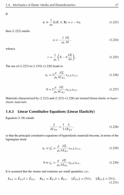
1.4. Mechanics of Elastic Media and Elastodynamics 37
If
ψ ≡ 1
ρ0(C, θ,X) = ε − θη, (1.223)
then (1.222) entails
η = − 1
ρ0
∂
∂θ, (1.224)
whence
ε = 1
ρ0
( − θ ∂
∂θ
), (1.225)
The use of (1.223) in (1.219)–(1.220) leads to
tkl = 2ρ
ρ0
∂
∂CKLx(k,Kxl),L, (1.226)
0 = 2ρ
ρ0
∂
∂CKLx[k,Kxl],L. (1.227)
Materials characterized by (1.212) and (1.223)–(1.226) are termed Green-elastic or hyper-elastic materials.
1.4.3 Linear Constitutive Equations (Linear Elasticity)
Equation (1.38) entails
∂
∂CKL= 1
2
∂
∂EKL, (1.228)
so that the principal constitutive equations of hyperelastic materials become, in terms of thelagrangian strain
tkl ≡ t+kl = ρ
ρ0
∂
∂EKLx(k,Kxl),L, (1.229)
0 ≡ t−kl = ρ
ρ0
∂
∂EKLx[k,Kxl],L. (1.230)
It is assumed that the strains and rotations are small quantities, i.e.,
EKL = EKLδ EKL, RKL = RKLδ RKL; ‖EKL‖ = O(1), ‖RKL‖ = O(1),(1.231)
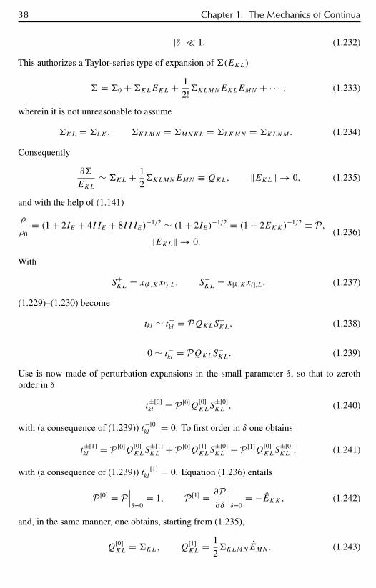
38 Chapter 1. The Mechanics of Continua
|δ| 1. (1.232)
This authorizes a Taylor-series type of expansion of (EKL)
= 0 +KLEKL + 1
2!KLMNEKLEMN + · · · , (1.233)
wherein it is not unreasonable to assume
KL = LK, KLMN = MNKL = LKMN = KLNM. (1.234)
Consequently
∂
EKL∼ KL + 1
2KLMNEMN ≡ QKL, ‖EKL‖ → 0, (1.235)
and with the help of (1.141)
ρ
ρ0= (1 + 2IE + 4IIE + 8IIIE)
−1/2 ∼ (1 + 2IE)−1/2 = (1 + 2EKK)
−1/2 ≡ P,‖EKL‖ → 0.
(1.236)
With
S+KL = x(k,Kxl),L, S−
KL = x[k,Kxl],L, (1.237)
(1.229)–(1.230) become
tkl ∼ t+kl = PQKLS+KL, (1.238)
0 ∼ t−kl = PQKLS−KL. (1.239)
Use is now made of perturbation expansions in the small parameter δ, so that to zerothorder in δ
t±[0]kl = P [0]Q[0]
KLS±[0]KL , (1.240)
with (a consequence of (1.239)) t−[0]kl = 0. To first order in δ one obtains
t±[1]kl = P [0]Q[0]
KLS±[1]KL + P [0]Q[1]
KLS±[0]KL + P [1]Q[0]
KLS±[0]KL , (1.241)
with (a consequence of (1.239)) t−[1]kl = 0. Equation (1.236) entails
P [0] = P∣∣∣δ=0
= 1, P [1] = ∂P∂δ
∣∣∣δ=0
= −EKK, (1.242)
and, in the same manner, one obtains, starting from (1.235),
Q[0]KL = KL, Q
[1]KL = 1
2KLMNEMN. (1.243)
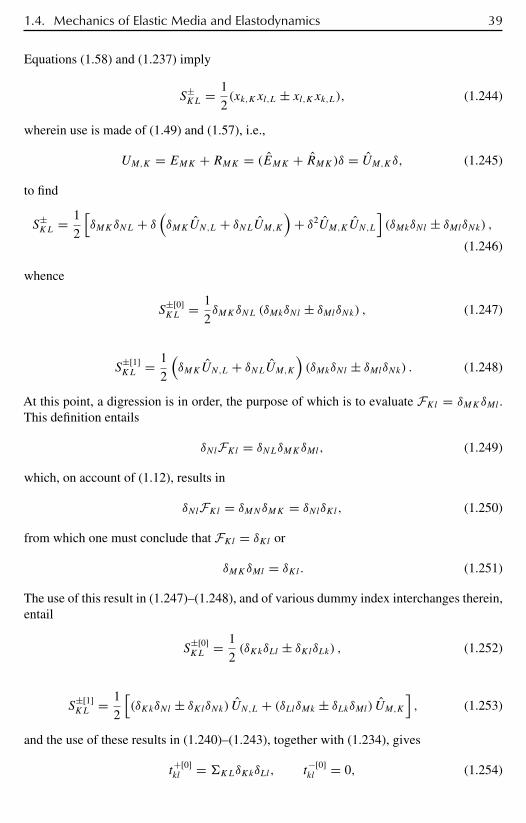
1.4. Mechanics of Elastic Media and Elastodynamics 39
Equations (1.58) and (1.237) imply
S±KL = 1
2(xk,Kxl,L ± xl,Kxk,L), (1.244)
wherein use is made of (1.49) and (1.57), i.e.,
UM,K = EMK + RMK = (EMK + RMK)δ = UM,Kδ, (1.245)
to find
S±KL = 1
2
[δMKδNL + δ
(δMKUN,L + δNLUM,K
)+ δ2UM,KUN,L
](δMkδNl ± δMlδNk) ,
(1.246)
whence
S±[0]KL = 1
2δMKδNL (δMkδNl ± δMlδNk) , (1.247)
S±[1]KL = 1
2
(δMKUN,L + δNLUM,K
)(δMkδNl ± δMlδNk) . (1.248)
At this point, a digression is in order, the purpose of which is to evaluate FKl = δMKδMl .This definition entails
δNlFKl = δNLδMKδMl, (1.249)
which, on account of (1.12), results in
δNlFKl = δMNδMK = δNlδKl, (1.250)
from which one must conclude that FKl = δKl or
δMKδMl = δKl. (1.251)
The use of this result in (1.247)–(1.248), and of various dummy index interchanges therein,entail
S±[0]KL = 1
2(δKkδLl ± δKlδLk) , (1.252)
S±[1]KL = 1
2
[(δKkδNl ± δKlδNk) UN,L + (δLlδMk ± δLkδMl) UM,K
], (1.253)
and the use of these results in (1.240)–(1.243), together with (1.234), gives
t+[0]kl = KLδKkδLl, t
−[0]kl = 0, (1.254)
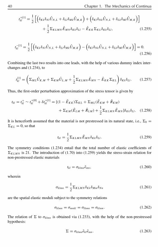
40 Chapter 1. The Mechanics of Continua
t+[1]kl = 1
2
[(δKkδNlUN,L + δLlδMkUM,K
)+(δKlδNkUN,L + δLkδMlUM,K
)]+ 1
2KLMNEMNδKkδLl − EKKKLδKkδLl, (1.255)
t−[1]kl = 1
2
[(δKkδNlUN,L + δLlδMkUM,K
)−(δKlδNkUN,L + δLkδMlUM,K
)]= 0.
(1.256)
Combining the last two results into one leads, with the help of various dummy index inter-changes and (1.234), to
t[1]kl =
(MLUK,M +KMUL,M + 1
2KLMNEMN − EKKKL
)δKkδLl. (1.257)
Thus, the first-order perturbation approximation of the stress tensor is given by
tkl = t+kl ∼ t+[0]kl + δt+[1]
kl = [(1 − EKK)KL +ML(EKM + RKM)+KM(ELM + RLM)+ 1
2KLMNEMN ]δKkδLl. (1.258)
It is henceforth assumed that the material is not prestressed in its natural state, i.e., 0 =KL = 0, so that
tkl = 1
2KLMNEMNδKkδLl. (1.259)
The symmetry conditions (1.234) entail that the total number of elastic coefficients ofKLMN is 21. The introduction of (1.70) into (1.259) yields the stress-strain relation fornon-prestressed elastic materials
tkl = σklmnemn, (1.260)
wherein
σklmn = 1
2KLMNδKkδMmδNn (1.261)
are the spatial elastic moduli subject to the symmetry relations
σklmn = σmnkl = σlkmn = σklnm. (1.262)
The relation of to σklmn is obtained via (1.233), with the help of the non-prestressedhypothesis:
= σklmnekl emn. (1.263)
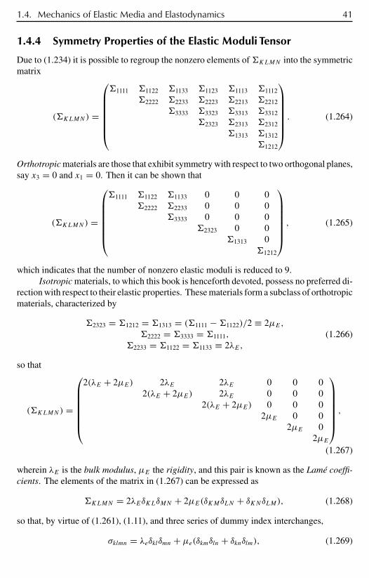
1.4. Mechanics of Elastic Media and Elastodynamics 41
1.4.4 Symmetry Properties of the Elastic Moduli Tensor
Due to (1.234) it is possible to regroup the nonzero elements ofKLMN into the symmetricmatrix
(KLMN) =
1111 1122 1133 1123 1113 1112
2222 2233 2223 2213 2212
3333 3323 3313 3312
2323 2313 2312
1313 1312
1212
. (1.264)
Orthotropic materials are those that exhibit symmetry with respect to two orthogonal planes,say x3 = 0 and x1 = 0. Then it can be shown that
(KLMN) =
1111 1122 1133 0 0 0
2222 2233 0 0 03333 0 0 0
2323 0 01313 0
1212
, (1.265)
which indicates that the number of nonzero elastic moduli is reduced to 9.Isotropic materials, to which this book is henceforth devoted, possess no preferred di-
rection with respect to their elastic properties. These materials form a subclass of orthotropicmaterials, characterized by
2323 = 1212 = 1313 = (1111 −1122)/2 ≡ 2µE,2222 = 3333 = 1111,
2233 = 1122 = 1133 ≡ 2λE,(1.266)
so that
(KLMN) =
2(λE + 2µE) 2λE 2λE 0 0 0
2(λE + 2µE) 2λE 0 0 02(λE + 2µE) 0 0 0
2µE 0 02µE 0
2µE
,(1.267)
wherein λE is the bulk modulus, µE the rigidity, and this pair is known as the Lamé coeffi-cients. The elements of the matrix in (1.267) can be expressed as
KLMN = 2λEδKLδMN + 2µE(δKMδLN + δKNδLM), (1.268)
so that, by virtue of (1.261), (1.11), and three series of dummy index interchanges,
σklmn = λeδklδmn + µe(δkmδln + δknδlm), (1.269)
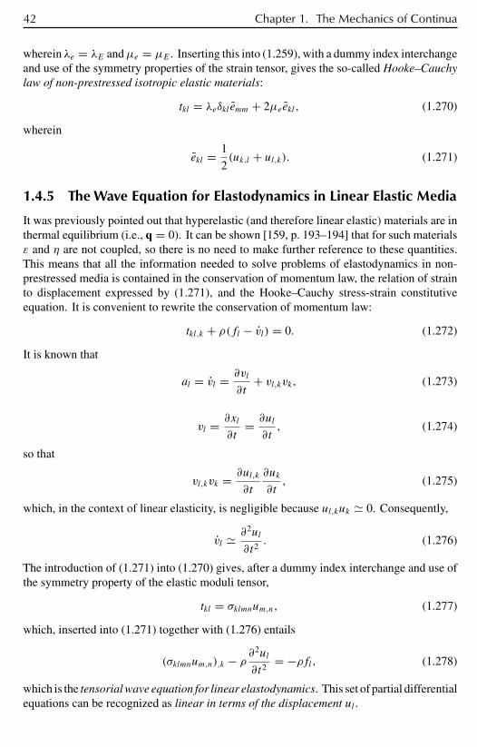
42 Chapter 1. The Mechanics of Continua
wherein λe = λE andµe = µE . Inserting this into (1.259), with a dummy index interchangeand use of the symmetry properties of the strain tensor, gives the so-called Hooke–Cauchylaw of non-prestressed isotropic elastic materials:
tkl = λeδkl emm + 2µeekl, (1.270)
wherein
ekl = 1
2(uk,l + ul,k). (1.271)
1.4.5 The Wave Equation for Elastodynamics in Linear Elastic Media
It was previously pointed out that hyperelastic (and therefore linear elastic) materials are inthermal equilibrium (i.e., q = 0). It can be shown [159, p. 193–194] that for such materialsε and η are not coupled, so there is no need to make further reference to these quantities.This means that all the information needed to solve problems of elastodynamics in non-prestressed media is contained in the conservation of momentum law, the relation of strainto displacement expressed by (1.271), and the Hooke–Cauchy stress-strain constitutiveequation. It is convenient to rewrite the conservation of momentum law:
tkl,k + ρ(fl − vl) = 0. (1.272)
It is known that
al = vl = ∂vl
∂t+ vl,kvk, (1.273)
vl = ∂xl
∂t= ∂ul
∂t, (1.274)
so that
vl,kvk = ∂ul,k
∂t
∂uk
∂t, (1.275)
which, in the context of linear elasticity, is negligible because ul,kuk 0. Consequently,
vl ∂2ul
∂t2. (1.276)
The introduction of (1.271) into (1.270) gives, after a dummy index interchange and use ofthe symmetry property of the elastic moduli tensor,
tkl = σklmnum,n, (1.277)
which, inserted into (1.271) together with (1.276) entails
(σklmnum,n),k − ρ ∂2ul
∂t2= −ρfl, (1.278)
which is the tensorial wave equation for linear elastodynamics. This set of partial differentialequations can be recognized as linear in terms of the displacement ul .

1.4. Mechanics of Elastic Media and Elastodynamics 43
1.4.6 Wave Equation for Elastodynamics in Compressible,Homogeneous Materials
This case corresponds to
σklmn,k = 0, (1.279)
so that (1.278) becomes
σklmnum,nk − ρ ∂2ul
∂t2= −ρfl. (1.280)
1.4.7 Wave Equation for Elastodynamics in Heterogeneous,Isotropic Solids
Starting from (1.269) it can be shown, with the help of a few dummy index interchanges,that
(σklmnum,n),k = λe,luk,k + (λe + µe)uk,kl + µeul,kk + µe,k(uk,l + ul,k), (1.281)
so that
(λe + µe)uk,kl + µeul,kk + λe,luk,k + µe,k(uk,l + ul,k)− ρ ∂2ul
∂t2= −ρfl. (1.282)
1.4.8 Wave Equation for Elastodynamics in Homogeneous,Isotropic Solids
The case of principal interest hereafter, that of waves in homogeneous (and isotropic) solids,is the one in which
λe,l = 0, µe,k = 0. (1.283)
The corresponding wave equation is
(λe + µe)uk,kl + µeul,kk − ρ ∂2ul
∂t2= −ρfl, (1.284)
which is known as Navier’s equation. Note that this equation is linear, like the wave equationfor acoustics in homogeneous fluids, but unlike the nonlinear Navier–Stokes equation.
By using (for any vector w)
wk,kl = (∇∇ · w)l, wl,kk = (∇2w)l, (1.285)
one obtains the vectorial form of Navier’s equation
µe∇2u + (λe + µe)∇∇ · u − ρ ∂2u∂t2
= −ρf . (1.286)

44 Chapter 1. The Mechanics of Continua
It proves useful to invoke the so-called Helmholtz decomposition of u and f [2, p. 85]
u = ∇φ + ∇ × ψ, f = ∇g + ∇ × h. (1.287)
Use is made of
∇∇ · ∇ × ψ = ∇(∇ · ∇ × ψ) = ∇(0) = 0,∇2∇ × ψ = ∇ × ∇2ψ,
∇2∇φ = ∇∇2φ,
∂2∇φ∂t2
= ∇ ∂2φ
∂t2,
∂2∇ × ψ
∂t2= ∇ × ∂2ψ
∂t2,
(1.288)
and of (1.283) to obtain
∇[µe∇2φ + (λe + µe)∇ · ∇φ − ρ ∂
2φ
∂t2+ ρg
]+ ∇ ×
[µe∇2ψ − ρ ∂
2ψ
∂t2+ ρh
]= 0,
(1.289)
which implies (for arbitrary u)
(λe + 2µe)∇2φ − ρ ∂2φ
∂t2= −ρg, (1.290)
µe∇2ψ − ρ ∂2ψ
∂t2= −ρh. (1.291)
These two relations can be written as
∇2φ − 1
c2p
∂2φ
∂t2= − 1
c2p
g, (1.292)
∇2ψ − 1
c2s
∂2ψ
∂t2= − 1
c2s
h, (1.293)
wherein
cp =√λe + 2µe
ρ, (1.294)
cs =õe
ρ< cp. (1.295)
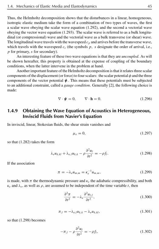
1.4. Mechanics of Elastic Media and Elastodynamics 45
Thus, the Helmholtz decomposition shows that the disturbances in a linear, homogeneous,isotropic elastic medium take the form of a combination of two types of waves, the firsta scalar wave obeying the scalar wave equation (1.292), and the second a vectorial waveobeying the vector wave equation (1.293). The scalar wave is referred to as a bulk longitu-dinal (or compressional) wave and the vectorial wave as a bulk transverse (or shear) wave.The longitudinal wave travels with the wavespeed cp and arrives before the transverse wave,which travels with the wavespeed cs (the symbols p, s designate the order of arrival, i.e.,p for primary, s for secondary).
An interesting feature of these two wave equations is that they are uncoupled. As willbe shown hereafter, this property is obtained at the expense of coupling of the boundaryconditions, when the latter intervene in the problem at hand.
Another important feature of the Helmholtz decomposition is that it relates three scalarcomponents of the displacement (or force) to four scalars: the scalar potentialφ and the threecomponents of the vector potential ψ . This means that these potentials must be subjectedto an additional constraint, called a gauge condition. Generally [2], the following choice ismade:
∇ · ψ = 0, ∇ · h = 0. (1.296)
1.4.9 Obtaining the Wave Equation of Acoustics in Heterogeneous,Inviscid Fluids from Navier’s Equation
In inviscid, linear, Stokesian fluids, the shear strain vanishes and
µe = 0, (1.297)
so that (1.282) takes the form
λeuk,kl + λe,luk,k − ρ ∂2ul
∂t2= −ρfl. (1.298)
If the association
π = −λeum,m = κ−1e um,m, (1.299)
is made, with π the thermodynamic pressure and κe the adiabatic compressibility, and bothκe and λe, as well as ρ, are assumed to be independent of the time variable t , then
∂2π
∂t2= −λe ∂
2ul,l
∂t2, (1.300)
π,l = −λe,luk,k − λeuk,kl, (1.301)
so that (1.298) becomes
−π,l − ρ ∂2ul
∂t2= −ρfl, (1.302)
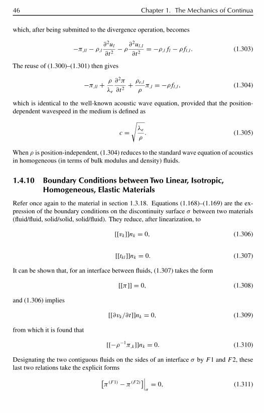
46 Chapter 1. The Mechanics of Continua
which, after being submitted to the divergence operation, becomes
−π,ll − ρ,l ∂2ul
∂t2− ρ ∂
2ul,l
∂t2= −ρ,lfl − ρfl,l . (1.303)
The reuse of (1.300)–(1.301) then gives
−π,ll + ρ
λe
∂2π
∂t2+ ρe,l
ρπ,l = −ρfl,l, (1.304)
which is identical to the well-known acoustic wave equation, provided that the position-dependent wavespeed in the medium is defined as
c =√λe
ρ. (1.305)
When ρ is position-independent, (1.304) reduces to the standard wave equation of acousticsin homogeneous (in terms of bulk modulus and density) fluids.
1.4.10 Boundary Conditions between Two Linear, Isotropic,Homogeneous, Elastic Materials
Refer once again to the material in section 1.3.18. Equations (1.168)–(1.169) are the ex-pression of the boundary conditions on the discontinuity surface σ between two materials(fluid/fluid, solid/solid, solid/fluid). They reduce, after linearization, to
[[vk]]nk = 0, (1.306)
[[tkl]]nk = 0. (1.307)
It can be shown that, for an interface between fluids, (1.307) takes the form
[[π ]] = 0, (1.308)
and (1.306) implies
[[∂vk/∂t]]nk = 0, (1.309)
from which it is found that
[[−ρ−1π,k]]nk = 0. (1.310)
Designating the two contiguous fluids on the sides of an interface σ by F1 and F2, theselast two relations take the explicit forms[
π(F1) − π(F2)]∣∣∣σ
= 0, (1.311)

1.4. Mechanics of Elastic Media and Elastodynamics 47[− 1
ρ(F1)π(F1),k + 1
ρ(F2)π(F2),k
]nk
∣∣∣σ
= 0. (1.312)
We recall (see sections 1.4.4 and 1.4.8) that for an arbitrary (solid or fluid), isotropic, elasticmaterial
tkl = λeδklum,m + µe(uk,l + ul,k
), (1.313)
and at points of space on which there are no applied forces, and in the neighborhood ofwhich the elastic material is homogeneous,
ρ∂vl
∂t= (λe + µe)uk,kl + µeul,kk, (1.314)
so that (1.307) and (1.309) take the forms
[[λeδklum,m + µe(uk,l + ul,k
)]]nk = 0, (1.315)
[[ρ−1(λe + µe)uk,kl + ρ−1µeul,kk]]nl = 0, (1.316)
which, for the interface between two contiguous solid media S1 and S2, become[λ(S1)e δklu
(S1)m,m + µ(S1)
e
(u(S1)k,l + u(S1)
l,k
)− λ(S2)
e δklu(S2)m,m − µ(S2)
e
(u(S2)k,l + u(S2)
l,k
)]nk
∣∣∣σ
= 0,
(1.317)
[λ(S1)e + µ(S1)
e
ρ(S1)u(S1)k,kl + µ(S1)
e
ρ(S1)u(S1)l,kk − λ(S2)
e + µ(S2)e
ρ(S2)u(S2)k,kl − µ(S2)
e
ρ(S2)u(S12)l,kk
]nl
∣∣∣σ
= 0. (1.318)
Combining these results, one obtains, on an interface between a fluid F1 and a solid S2,[−π(F1)δkl − λ(S2)
e δklu(S2)m,m − µ(S2)
e
(u(S2)k,l + u(S2)
l,k
)]nk
∣∣∣σ
= 0, (1.319)
[− 1
ρ(F1)π(F1),l − λ(S2)
e + µ(S2)e
ρ(S2)u(S2)k,kl − µ(S2)
e
ρ(S2)u(S12)l,kk
]nl
∣∣∣σ
= 0. (1.320)
The following limit cases, of considerable mathematical (if not physical) interest, are easilyderivable from the preceding relations:
π(F1)∣∣∣σ
= 0 (1.321)
for a fluid/acoustically soft material interface, the pressure being negligible in the acousti-cally soft material;
π(F1),k nk
∣∣∣σ
= 0 (1.322)

48 Chapter 1. The Mechanics of Continua
for a fluid/acoustically hard material interface, the velocity being negligible in the acousti-cally soft material; [
λ(S1)e + µ(S1)
e
ρ(S1)u(S1)k,kl + µ(S1)
e
ρ(S1)u(S1)l,kk
]nl
∣∣∣σ
= 0 (1.323)
for a solid/rigid solid (in which the displacement is negligible) interface;[λ(S1)e δklu
(S1)m,m + µ(S1)
e
(u(S1)k,l + u(S1)
l,k
)]nl
∣∣∣σ
= 0 (1.324)
for a solid/vacuum (in which the stress is negligible) interface,[α(λeδklu
(1)m,m + µ(1)e
(u(1)k,l + u(1)l,k
))+ β
(λ(S1)e + µ(S1)
e
ρ(S1)u(S1)k,kl + µ(S1)
e
ρ(S1)u(S1)l,kk
)]nl
∣∣∣σ
= 0,
(1.325)
corresponding to the so-called impedance or Robin boundary condition (in which α and βare arbitrary real coefficients) of which the relations (1.323) and (1.324) are special cases (inall three cases, expressed by (1.323)–(1.325), the stress and/or displacement are assumedto be negligible in the second medium).
It is also possible to account for applied (and therefore assumed known) accelerationor stress on a portion σ (a) of σ :[
λ(S1)e + µ(S1)
e
ρ(S1)u(S1)k,kl + µ(S1)
e
ρ(S1)u(S1)l,kk
]nl
∣∣∣σ (a)
=(∂vl
∂t
)(a)(1.326)
for known applied acceleration on σ (a) (the other conditions being the previously evokedones on σ − σ (a)) and[
λeδklu(1)m,m + µ(1)e
(u(1)k,l + u(1)l,k
)]nk
∣∣∣σ (a)
= t(a)kl (1.327)
for known applied stress on σ (a) (the other conditions being the previously evoked ones onσ − σ (a)). Formulas equivalent to (1.323)–(1.327) in terms of velocity and pressure can beobtained for the case in which the adjoining media are both fluids.
1.5 Forward and Inverse Wavefield Problems
1.5.1 Introduction
The fundamental ingredients of the forward and inverse wavefield problems considered inthis book are (i) the system of partial differential equations (PDEs) for the wavefield, (ii) theboundary conditions (BCs), and (iii) the radiation conditions at infinity (RCIs) in case thespatial domain in which the solution sought is infinite.
Since waves are spatiotemporal phenomena, they are treated, in the most natural way,in the space-time framework. The PDEs and BCs for this type of analysis were given in thepreceding sections.
1.5. Forward and Inverse Wavefield Problems 49
It often proves useful to analyze the problem in the space-frequency framework—notably for treating wave phenomena in dissipative media. This is done by Fourier trans-formation of the space-time PDEs, BCs, and RCIs and will be described in subsequentsections.
Since wave motion in the sea environment corresponds to many particular situations,the governing equations of only a few of these situations will be given in the remainder ofthis chapter. The others will be described in the applications part of this book (Chapters 2–5).
Referring to the material in section 1.4.9, recall that f , π , and u are generally functionsof x and t , whereas c, λe, µe, and ρ are generally functions of position x = (x1, x2, . . . , xn)
(with n the dimension of the considered space), but not of t . The following symbol replace-ments will be made to conform with the usual notations:
p(x, t) ≡ π,
λ(x) ≡ λe,
µ(x) ≡ µe.
(1.328)
1.5.2 The Frequency-Domain Equation for Propagation in anUnbounded, Heterogeneous, Inviscid Fluid Medium
Recall that the density is assumed not to depend on time t . The pressure and applied forceare expressed by the Fourier integrals
p(x, t) =∫ ∞
−∞p(x, ω) exp(−iωt)dω, (1.329)
fl(x, t) =∫ ∞
−∞fl(x, ω) exp(−iωt)dω, (1.330)
and since p(x, t) and fl(x, t) are real functions, it is readily shown that
p(x,−ω) = p∗(x, ω), fl(x,−ω) = f ∗l (x, ω), (1.331)
wherein the symbol ∗ signifies the complex conjugate operator, so that
p(x, t) = 2∫ ∞
0p(x, ω) exp(−iωt)dω, (1.332)
fl(x, t) = 2∫ ∞
0fl(x, ω) exp(−iωt)dω, (1.333)
wherein signifies “real part of.’’ In spite of this latter result, it is preferable to employ(1.329)–(1.330), with the understanding that p(x, ω) and fl(x, ω) obey (1.331).
The introduction of (1.329)–(1.330) into the time-domain wave equation gives (afterinterchange of integration and differentiation operators)∫ ∞
−∞
[−p,ll(x, ω)− ω2
c2(x)p(x, ω)+ ρ,l(x)
ρ(x)p,l(x, ω)+ ρ(x)fl,l(x, ω)
]exp(−iωt)dω = 0
∀x ∈ Rn, ∀t > 0. (1.334)
50 Chapter 1. The Mechanics of Continua
This relation can be true for all t > 0 only if [ . ] = 0, which means that
−p,ll(x, ω)− ω2
c2(x)p(x, ω)+ ρ,l(x)
ρ(x)p,l(x, ω) = −ρ(x)fl,l(x, ω) ∀x ∈ Rn, ∀ω ∈ R.
(1.335)
This is the sought-after frequency-domain wave equation (also termed the inhomogeneousHelmholtz equation) in heterogeneous fluids.
1.5.3 The Frequency-Domain Radiation Condition at Infinity
It is assumed that (i) space is divided into a bounded (inner) domainin and an unbounded(outer) domain out , (ii) the origin o of a euclidian reference system ox1x2x3 is entirelywithin in, (iii) the support of the sources of the wavefield is entirely within in, and(iv) the medium filling in is generally heterogeneous, whereas the medium filling out ishomogeneous. One can show, as in the previous section, that the frequency-domain waveequation in out (which, it is recalled, is homogeneous, and wherein the wavespeed is theconstant c) satisfied by the scalar potential φ and the three scalar components of the vectorpotential ψ (in an elastic solid) is of the generic form
w,ll(x, ω)+ ω2
c2w(x, ω) = 0 ∀x ∈ out , ∀ω ∈ R. (1.336)
The case of a 3D space is treated first. A plausible guess is that the asymptotic solutions for
large ‖x‖ =√x2
1 + x22 + x2
3 are of the form
w(x, ω) ∼ w±(x, ω) ≡ 1
‖x‖ exp(±ik · x), (1.337)
wherein
k = ω
ck, ‖k‖ = 1, i ≡ √−1. (1.338)
One finds that
w,ll(x, ω)+ ω2
c2w(x, ω) ∼ ±i k · x
‖x‖3exp(±ik · x)→ 0, ‖x‖ → ∞, (1.339)
which shows that the two functions w± written in (1.337) are indeed asymptotic solutions,for large |x‖, of the frequency-domain wave equation (1.336).
One can write
w±(x, t) ∼∫ ∞
∞w±(x, ω) exp(−iωt)dω =
∫ ∞
∞1
‖x‖ exp[i(±k · x − ωt)]dω
=∫ ∞
∞1
‖x‖ exp[i(±ωc
k · x − ωt)]dω. (1.340)
1.5. Forward and Inverse Wavefield Problems 51
The only way to ensure compatibility with the solution satisfying the time-domain radiation(i.e., outgoing wave) condition at infinity (TDRCI) is by choosing w+(x, ω) instead ofw−(x, ω). Thus, in three dimensions, the frequency-domain radiation condition at infinity(FDRCI) amounts to the choice
w(x, ω) ∼ w+(x, ω) = 1
‖x‖ exp(ik · x), ‖x‖ → ∞. (1.341)
In the same manner one can show that the 2D version of the FDRCI corresponds to thechoice
w(x, ω) ∼ w+(x, ω) = 1√‖x‖ exp(ik · x), ‖x‖ → ∞, (1.342)
wherein x = x1i1 + x2i2.
1.5.4 Governing Equations for the Frequency-Domain Formulationof Wave Propagation in an Unbounded, Heterogeneous,Inviscid Fluid Medium
It was already shown that the PDE of this problem (see (1.335)) is
−p,ll(x, ω)− ω2
c2(x)p(x, ω)+ ρ,l(x)
ρ(x)p,l(x, ω) = −ρ(x)fl,l(x, ω) ∀x ∈ Rn, ∀ω ∈ R.
(1.343)
There are no initial conditions to cope with in the frequency domain since this is a permanentregime. The only remaining condition is the RCI, which takes the following form:
p(x, ω) satisfies the FDRCI: ‖x‖ → ∞ ∀ x‖x‖ , ∀ω ∈ R. (1.344)
1.5.5 Governing Equations for the Frequency-Domain Formulationof Wave Propagation in Two Contiguous, Semi-Infinite,Heterogeneous, Inviscid Fluid Media
The media are the same as in section 1.5.2, so that the governing equations are (after useof (1.329))
− p(F1),ll (x, ω)−
ω2(c(F1)(x)
)2p(F1)(x, ω)+ ρ
(F1),l (x)
ρ(F1)(x)p(F1),l (x, ω) = −ρ(F1)(x)fl,l(x, ω)
∀x ∈ (F1), ∀ω ∈ R, (1.345)
− p(F2),ll (x, ω)−
ω2(c(F2)(x)
)2p(F2)(x, ω)+ ρ
(F2),l (x)
ρ(F2)(x)p(F2),l (x, ω) = −ρ(F2)(x)fl,l(x, ω)
∀x ∈ (F2), ∀ω ∈ R, (1.346)
52 Chapter 1. The Mechanics of Continua
[p(F1)(x, ω)− p(F2)(x, ω)
]∣∣∣σ
= 0 ∀ω ∈ R, (1.347)
[1
ρ(F1)p(F1),k (x, ω)− 1
ρ(F2)p(F2),k (x, ω)
]nk
∣∣∣σ
= 0 ∀ω ∈ R, (1.348)
p(F1)(x, ω) satisfies the FDRCI: ‖x‖ → ∞ ∀ x‖x‖ such that x ∈ (F1) ∀ω ∈ R,
(1.349)
p(F2)(x, t) satisfies the FDRCI: ‖x‖ → ∞ ∀ x‖x‖ such that x ∈ (F2) ∀ω ∈ R.
(1.350)
When the domain occupied by the second fluid medium is bounded, the governing equationsare the same as above, and the radiation condition (1.350) becomes superfluous.
1.5.6 Governing Equations for the Frequency-Domain Formulationof Wave Propagation in an Unbounded, Heterogeneous,Isotropic, Elastic Solid
The configuration is the same as in section 1.4.7, so that the governing equations are (afteruse of a Fourier transform such as (1.329))
[λ(x)+ µ(x)] uk,kl(x, ω)+ µ(x)ul,kk(x, ω)+ λ,l(x)uk,k(x, ω)+ µ,k(x)
[uk,l(x, ω)+ ul,k(x, t)
]+ ρ(x)ω2ul(x, ω) = −ρ(x)fl(x, ω)∀x ∈ Rn, ∀ω ∈ R, (1.351)
uk(x, ω) satisfies the FDRCI: ‖x‖ → ∞ ∀ω ∈ R. (1.352)
1.5.7 Governing Equations for the Frequency-Domain Formulationof Wave Propagation in Two Semi-Infinite, Heterogeneous,Isotropic, Elastic Solid Media in Welded Contact
The media are the same as in section 1.5.6, so that the governing equations are (after use of(1.329))[
λ(S1)(x)+ µ(S1)(x)]u(S1)k,kl (x, ω)+ µ(S1)(x)u(S1)
l,kk (x, ω)+ λ(S1),l (x)u(S1)
k,k (x, ω)
+ µ(S1),k (x)
[u(S1)k,l (x, ω)+ u(S1)
l,k (x, ω)]+ ρ(S1)(x)ω2u
(S1)l (x, ω)
= −ρ(S1)(x)f (S1)l (x, ω) ∀x ∈ (S1), ∀ω ∈ R, (1.353)
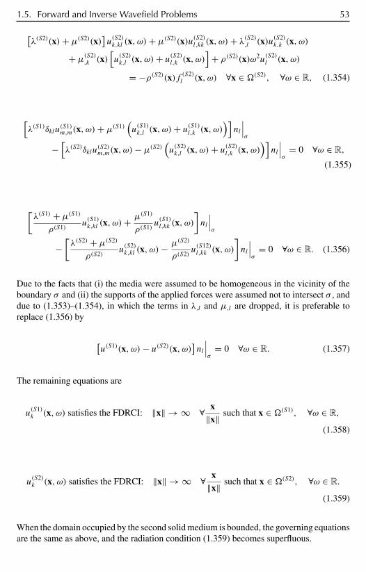
1.5. Forward and Inverse Wavefield Problems 53
[λ(S2)(x)+ µ(S2)(x)
]u(S2)k,kl (x, ω)+ µ(S2)(x)u(S2)
l,kk (x, ω)+ λ(S2),l (x)u(S2)
k,k (x, ω)
+ µ(S2),k (x)
[u(S2)k,l (x, ω)+ u(S2)
l,k (x, ω)]+ ρ(S2)(x)ω2u
(S2)l (x, ω)
= −ρ(S2)(x)f (S2)l (x, ω) ∀x ∈ (S2), ∀ω ∈ R, (1.354)
[λ(S1)δklu
(S1)m,m(x, ω)+ µ(S1)
(u(S1)k,l (x, ω)+ u(S1)
l,k (x, ω))]nl
∣∣∣σ
−[λ(S2)δklu
(S2)m,m(x, ω)− µ(S2)
(u(S2)k,l (x, ω)+ u(S2)
l,k (x, ω))]nl
∣∣∣σ
= 0 ∀ω ∈ R,
(1.355)
[λ(S1) + µ(S1)
ρ(S1)u(S1)k,kl (x, ω)+
µ(S1)
ρ(S1)u(S1)l,kk (x, ω)
]nl
∣∣∣σ
−[λ(S2) + µ(S2)
ρ(S2)u(S2)k,kl (x, ω)−
µ(S2)
ρ(S2)u(S12)l,kk (x, ω)
]nl
∣∣∣σ
= 0 ∀ω ∈ R. (1.356)
Due to the facts that (i) the media were assumed to be homogeneous in the vicinity of theboundary σ and (ii) the supports of the applied forces were assumed not to intersect σ , anddue to (1.353)–(1.354), in which the terms in λ,l and µ,l are dropped, it is preferable toreplace (1.356) by
[u(S1)(x, ω)− u(S2)(x, ω)
]nl
∣∣∣σ
= 0 ∀ω ∈ R. (1.357)
The remaining equations are
u(S1)k (x, ω) satisfies the FDRCI: ‖x‖ → ∞ ∀ x
‖x‖ such that x ∈ (S1), ∀ω ∈ R,
(1.358)
u(S2)k (x, ω) satisfies the FDRCI: ‖x‖ → ∞ ∀ x
‖x‖ such that x ∈ (S2), ∀ω ∈ R.
(1.359)
When the domain occupied by the second solid medium is bounded, the governing equationsare the same as above, and the radiation condition (1.359) becomes superfluous.
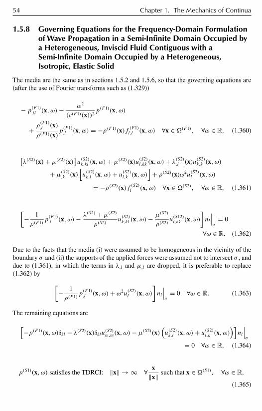
54 Chapter 1. The Mechanics of Continua
1.5.8 Governing Equations for the Frequency-Domain Formulationof Wave Propagation in a Semi-Infinite Domain Occupied bya Heterogeneous, Inviscid Fluid Contiguous with aSemi-Infinite Domain Occupied by a Heterogeneous,Isotropic, Elastic Solid
The media are the same as in sections 1.5.2 and 1.5.6, so that the governing equations are(after the use of Fourier transforms such as (1.329))
− p(F1),ll (x, ω)−
ω2
(c(F1)(x))2p(F1)(x, ω)
+ ρ(F1),l (x)
ρ(F1)(x)p(F1),l (x, ω) = −ρ(F1)(x)f (F1)
l,l (x, ω) ∀x ∈ (F1), ∀ω ∈ R, (1.360)
[λ(S2)(x)+ µ(S2)(x)
]u(S2)k,kl (x, ω)+ µ(S2)(x)u(S2)
l,kk (x, ω)+ λ(S2),l (x)u(S2)
k,k (x, ω)
+ µ(S2),k (x)
[u(S2)k,l (x, ω)+ u(S2)
l,k (x, ω)]+ ρ(S2)(x)ω2u
(S2)l (x, ω)
= −ρ(S2)(x)f (S2)l (x, ω) ∀x ∈ (S2), ∀ω ∈ R, (1.361)
[− 1
ρ(F1)p(F1),l (x, ω)− λ(S2) + µ(S2)
ρ(S2)u(S2)k,kl (x, ω)−
µ(S2)
ρ(S2)u(S12)l,kk (x, ω)
]nl
∣∣∣σ
= 0
∀ω ∈ R. (1.362)
Due to the facts that the media (i) were assumed to be homogeneous in the vicinity of theboundary σ and (ii) the supports of the applied forces were assumed not to intersect σ , anddue to (1.361), in which the terms in λ,l and µ,l are dropped, it is preferable to replace(1.362) by [
− 1
ρ(F1)p(F1),l (x, ω)+ ω2u
(S2)l (x, ω)
]nl
∣∣∣σ
= 0 ∀ω ∈ R. (1.363)
The remaining equations are
[−p(F1)(x, ω)δkl − λ(S2)(x)δklu(S2)
m,m(x, ω)− µ(S2)(x)(u(S2)k,l (x, ω)+ u(S2)
l,k (x, ω))]nl
∣∣∣σ
= 0 ∀ω ∈ R, (1.364)
p(S1)(x, ω) satisfies the TDRCI: ‖x‖ → ∞ ∀ x‖x‖ such that x ∈ (S1), ∀ω ∈ R,
(1.365)
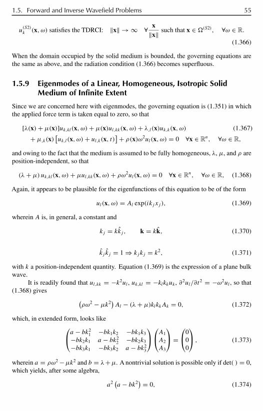
1.5. Forward and Inverse Wavefield Problems 55
u(S2)k (x, ω) satisfies the TDRCI: ‖x‖ → ∞ ∀ x
‖x‖ such that x ∈ (S2), ∀ω ∈ R.
(1.366)
When the domain occupied by the solid medium is bounded, the governing equations arethe same as above, and the radiation condition (1.366) becomes superfluous.
1.5.9 Eigenmodes of a Linear, Homogeneous, Isotropic SolidMedium of Infinite Extent
Since we are concerned here with eigenmodes, the governing equation is (1.351) in whichthe applied force term is taken equal to zero, so that
[λ(x)+ µ(x)]uk,kl(x, ω)+ µ(x)ul,kk(x, ω)+ λ,l(x)uk,k(x, ω) (1.367)
+ µ,k(x)[uk,l(x, ω)+ ul,k(x, t)
]+ ρ(x)ω2ul(x, ω) = 0 ∀x ∈ Rn, ∀ω ∈ R,
and owing to the fact that the medium is assumed to be fully homogeneous, λ, µ, and ρ areposition-independent, so that
(λ+ µ) uk,kl(x, ω)+ µul,kk(x, ω)+ ρω2ul(x, ω) = 0 ∀x ∈ Rn, ∀ω ∈ R, (1.368)
Again, it appears to be plausible for the eigenfunctions of this equation to be of the form
ul(x, ω) = Al exp(ikjxj ), (1.369)
wherein A is, in general, a constant and
kj = kkj , k = kk, (1.370)
kj kj = 1 ⇒ kj kj = k2, (1.371)
with k a position-independent quantity. Equation (1.369) is the expression of a plane bulkwave.
It is readily found that ul,kk = −k2ul , uk,kl = −klkkuk , ∂2ul/∂t2 = −ω2ul , so that
(1.368) gives (ρω2 − µk2
)Al − (λ+ µ)klkkAk = 0, (1.372)
which, in extended form, looks likea − bk21 −bk1k2 −bk1k3
−bk2k1 a − bk22 −bk2k3
−bk3k1 −bk3k2 a − bk23
A1
A2
A3
=0
00
, (1.373)
wherein a = ρω2 −µk2 and b = λ+µ. A nontrivial solution is possible only if det( ) = 0,which yields, after some algebra,
a2(a − bk2
) = 0, (1.374)
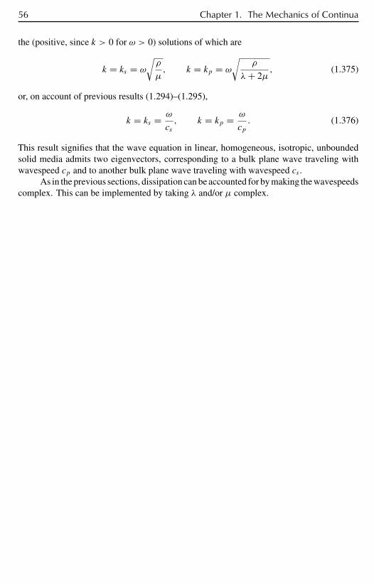
56 Chapter 1. The Mechanics of Continua
the (positive, since k > 0 for ω > 0) solutions of which are
k = ks = ω
√ρ
µ, k = kp = ω
√ρ
λ+ 2µ, (1.375)
or, on account of previous results (1.294)–(1.295),
k = ks = ω
cs, k = kp = ω
cp. (1.376)
This result signifies that the wave equation in linear, homogeneous, isotropic, unboundedsolid media admits two eigenvectors, corresponding to a bulk plane wave traveling withwavespeed cp and to another bulk plane wave traveling with wavespeed cs .
As in the previous sections, dissipation can be accounted for by making the wavespeedscomplex. This can be implemented by taking λ and/or µ complex.
Chapter 2
Direct Scattering Problemsin Ocean Environments
2.1 The Constant Depth, Homogeneous OceanIn Chapters 2 and 3 we consider in mathematical detail the direct and inverse scatteringproblems for an object in a wave guide.
2.1.1 Point Source Response in a Constant Depth, HomogeneousOcean
In a homogeneous ocean of constant depth, the response to the point source time-harmonicacoustic wave (Green’s function) satisfies the nonhomogeneous equation
G+ k2G = −δ(z− z0)δ(r)
2πr. (2.1)
Here, the source is located at (x0, 0) in a cylindrical coordinate system, where 3 isthe 3D Laplace operator.
Assuming the ocean to be of constant depth h, the surface conditions are
G = 0 at the surface z = 0 and∂G
∂z= 0 at the bottom at z = h. (2.2)
z = 0 is referred to as a pressure-release boundary, and z = h is a totally reflecting boundary.Using the method of separation of variables with the boundary conditions (2.2), we mayrepresent the Green’s function as
G(r, z; 0, z0) =∞∑n=0
φn(z)ψn(r)
=∞∑n=0
φn(z)[anH
(1)0 (kanr)+ bnH(2)
0 (kanr)],
57
58 Chapter 2. Direct Scattering Problems in Ocean Environments
where H(1)0 and H(2)
0 are Hankel functions of order zero of the first and second kind, re-spectively. Since we restrict our attention to outgoing waves, the appropriate form of theradiation condition is
limr→∞ r
1/2
(∂ψn
∂r− ikanψn
)= 0. (2.3)
Here the coefficients an are the eigenvalues of the separated modal solutions φn, i.e.,
an =[
1 − (2n+ 1)2π2
4k2h2
]1/2
, (2.4)
φn(z) = sin[k(1 − a2n)
1/2z]. (2.5)
Throughout this book, we shall refer to this condition (and some of its variations) as theoutgoing radiation condition, and the corresponding Green’s function shall be referred toas the outgoing Green’s function. The outgoing Green’s function has several equivalentrepresentations [6], including the normal mode representation
G(r, z; 0, z0) = i
2h
∞∑n=0
φn(z)φn(z0)H(1)0 (kanr) (2.6)
and the integral representation
G(r, z; 0, z0) = − k
2π
∫ ∞
0J0(kar)
sin(k√k(1 − a2)z>
)cos
(k√k(1 − a2)z<
)√
1 − a2 cos(k√k(1 − a2)
) da.
(2.7)
2.1.2 Propagating Solutions in an Ocean with Sound-Soft Obstacle
In this section we use the methods of integral equations to solve the direct scattering problemfor the reduced wave equation.2 Integral equation methods are powerful tools for theinvestigation of the boundary value problems associated with the scattering of waves bybounded obstacles. For simplicity we concentrate on scattering surfaces that are smooth,say at least twice continuously differentiable. The reader may find further details concerningthe regularity properties of surface potentials corresponding to nonsmooth surfaces in [125].
We suppose that the ocean occupies the space given by R3h = (x, z) ∈ R3; x =
(x1, x2) ∈ R2, 0 ≤ z ≤ h, h being the ocean depth. The submerged object occupies thespace ⊂⊂ R3
h, a bounded domain with aC2 boundary. The outward-pointing unit normalis denoted by ν. Without loss of generality, it may be assumed that (0, z0) ∈ for somez0 ∈ [0, h].
2In this and subsequent chapters, unless otherwise stated we shall restrict our attention to the case of a finite,homogeneous ocean.
2.1. The Constant Depth, Homogeneous Ocean 59
In this and subsequent chapters we retain the following notation:
R := (y, ζ ) ∈ R3h; |y| < R, R := ∂R,
CR = (y, ζ ) ∈ R3h; |y| = R,
SR = (x, 0) ∈ R3h; |x| ≤ R, BR = (x, h) ∈ R3
h; |x| ≤ R,
eR = (x, z) ∈ R3h \; |x| ≤ R, e = R3
h \.The direct scattering problem in a constant depth, homogeneous ocean with a pressure-release surface and a rigid bottom may be formulated as seeking a function u ∈ C2(R3
h \) ∩ C(R3
h \) such that u satisfies the Helmholtz equation
3u+ k2u = 0 in R3h \, (2.8)
with the pressure-release condition, the completely reflecting bottom, and the outgoingradiation condition. Moreover, on the submerged object the boundary condition
u = g(x, z) for (x, z) ∈ ∂ (2.9)
holds.It is well known that u has a normal mode representation
u =∞∑n=0
un(x, z) =∞∑n=0
φn(z)un(x) for |x| ≥ R, (2.10)
whereun(x) is thenth Fourier coefficient with respect to the eigenfunctionφn, which satisfiesoutgoing radiation condition
limr→∞ r
1/2
(∂un
∂r− ikanun
)= 0 (2.11)
uniformly for θ ∈ [0, 2π), where r = |x| and θ = tan−1( x2x1). The constant R is chosen so
that ⊂ R [6].We will refer to the problem described by (2.8), (2.2), (2.9), (2.10), (2.11) as Prob-
lem D.
2.1.3 The Representation of Propagating Solutions
If u is a solution of Problem D in C2(R3h \)∩C(R3
h \), such that the normal derivativeon the boundary exists in the sense that the limit
∂u
∂ν(x, z) = lim
δ→0(ν(x, z), grad u(x, z)− δν(x, z)) , (x, z) ∈ ∂,

60 Chapter 2. Direct Scattering Problems in Ocean Environments
exists uniformly on ∂, then it follows by Green’s identity that∫R
G(z, ζ, |x − ξ |)∂u(ξ, ζ )
∂ν− ∂G
∂ν(z, ζ, |x − ξ |)u(ξ, ζ )
dσ
−∫∂
G(z, ζ, |x − ξ |)∂u(ξ, ζ )
∂ν− ∂G
∂ν(z, ζ, |x − ξ |)u(ξ, ζ )
dσ
=
0 if (x, z) ∈ ,− ∫
εG(z, ζ, |x − ξ |) ∂u(ξ,ζ )
∂ν− ∂G
∂ν(z, ζ, |x − ξ |)u(ξ, ζ )dσ, (2.12)
if (x, z) ∈ R3h \.
Here G is the Green’s function defined in section 2.1.1, and
ε := (y, ζ ); [|y − x|2 + (ζ − z)2]1/2 < εrepresents an ε-neighborhood of (x, z); moreover,ε := ∂ε, and ε, R are positive numberssuch that ε ⊂ R3
h \, ⊂ R .It is clear that we can separate the polar singularity of G(z, ζ, |x − ξ |) [6] into the
form
G(z, ζ, |x − ξ |) = eik√
|x−ξ |2+(z−ζ )2
4π√
|x − ξ |2 + (z− ζ )2+1(z, ζ, |x − ξ |), (2.13)
where the regular part is given by
1(z, ζ, |x − ξ |)
= 1
4π
∞∑n=−∞,n=0
eik
√|x−ξ |2+(z−ζ−2nh)2√|x − ξ |2 + (z− ζ − 2nh)2
− eik√
|x−ξ |2+(z+ζ−2nh)2√|x − ξ |2 + (z+ ζ − 2nh)2
− eik√
|x−ξ |2+(z+ζ )2
4π√
|x − ξ |2 + (z+ ζ )2.
Moreover, 1(z, ζ, |x − ξ |) is bounded and continuous at z = ζ, x = ξ . It is easily seenthat ∫
ε
G∂u
∂νdσ → 0
and ∫ε
u∂G
∂νdσ → u(x, z) as ε → 0.
2.1. The Constant Depth, Homogeneous Ocean 61
From (2.12) and using (2.2), (2.9), (2.10), we thereby obtain∫CR
G∂u
∂ν− ∂G
∂νu
dσ −
∫∂
G∂u
∂ν− ∂G
∂νu
dσ
=
0 if (x, z) ∈ ,u(x, z) if (x, z) ∈ R3
h \.
Using the radiation condition (2.11) and the fact that H(1)0 (kan|x − ξ |) = 0( 1
r1/2 ), asr → ∞, it is easy to see that [467]∫
CR
G∂u
∂r− ikGu
dσ → 0 as R → ∞.
Therefore, we may conclude that if u ∈ C2(R3h \ ) ∩ C(R3
h \ ) is a solution toProblem D, then∫
∂
u∂G
∂ν−G∂u
∂ν
dσ =
0 if (x, z) ∈ ,u(x, z) if (x, z) ∈ R3
h \. (2.14)
Remark. Since G(z, ζ, |x − ξ |) satisfies the radiation condition, u(x, z) must alsosatisfy the same condition.
2.1.4 The Uniqueness Theorem for the Dirichlet Problem
In order to show that our problem has a solution that uniquely depends on the boundarydata, we need to show that the problem with homogeneous data has the trivial solution. Inother words, we want to show that if u ∈ C2(R3
h \ ) ∩ C(R3h \ ) is a solution of the
homogeneous Problem D and k = (2n+ 1)π/2h for n = 0, 1, . . . , then u ≡ 0 in R3h \.
We will prove this in several steps.
Lemma 2.1. If u ∈ C2(R3h \)∩C(R3
h \) is a solution of Problem D with homogeneousboundary data g = 0, then for any R > 0 such that R ⊃
∞∑n=0
Im∫ 2π
0
[un∂un
∂r
]r=R
R dθ = 0,
when un is the nth normal mode of the solution.
Proof. By Green’s identity, we have∫∂∪CR
(u∂u
∂ν− u∂u
∂ν
)dσ =
∫R\
(u u− u u) dX
=∫R\
(k
2|u|2 − k2|u|2)dX = 0.
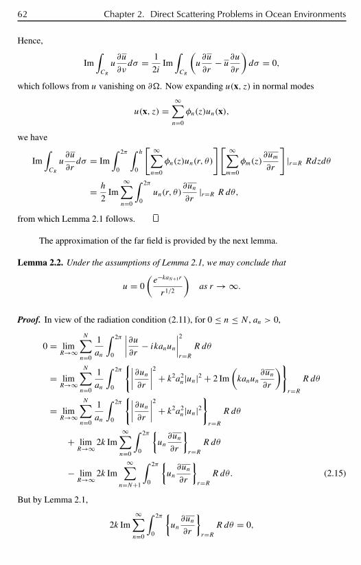
62 Chapter 2. Direct Scattering Problems in Ocean Environments
Hence,
Im∫CR
u∂u
∂νdσ = 1
2iIm
∫CR
(u∂u
∂r− u∂u
∂r
)dσ = 0,
which follows from u vanishing on ∂. Now expanding u(x, z) in normal modes
u(x, z) =∞∑n=0
φn(z)un(x),
we have
Im∫CR
u∂u
∂rdσ = Im
∫ 2π
0
∫ h
0
[ ∞∑n=0
φn(z)un(r, θ)
][ ∞∑m=0
φm(z)∂um
∂r
]|r=R Rdzdθ
= h
2Im
∞∑n=0
∫ 2π
0un(r, θ)
∂un
∂r|r=R R dθ,
from which Lemma 2.1 follows.
The approximation of the far field is provided by the next lemma.
Lemma 2.2. Under the assumptions of Lemma 2.1, we may conclude that
u = 0
(e−kaN+1r
r1/2
)as r → ∞.
Proof. In view of the radiation condition (2.11), for 0 ≤ n ≤ N , an > 0,
0 = limR→∞
N∑n=0
1
an
∫ 2π
0
∣∣∣∣∂u∂r − ikanun∣∣∣∣2r=R
R dθ
= limR→∞
N∑n=0
1
an
∫ 2π
0
∣∣∣∣∂un∂r∣∣∣∣2 + k2a2
n|un|2 + 2 Im
(kanun
∂un
∂r
)r=R
R dθ
= limR→∞
N∑n=0
1
an
∫ 2π
0
∣∣∣∣∂un∂r∣∣∣∣2 + k2a2
n|un|2r=R
R dθ
+ limR→∞ 2k Im
∞∑n=0
∫ 2π
0
un∂un
∂r
r=R
R dθ
− limR→∞ 2k Im
∞∑n=N+1
∫ 2π
0
un∂un
∂r
r=R
R dθ. (2.15)
But by Lemma 2.1,
2k Im∞∑n=0
∫ 2π
0
un∂un
∂r
r=R
R dθ = 0,
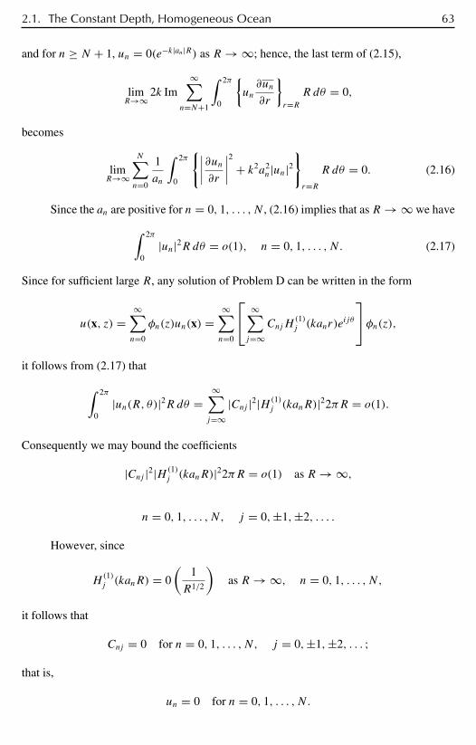
2.1. The Constant Depth, Homogeneous Ocean 63
and for n ≥ N + 1, un = 0(e−k|an|R) as R → ∞; hence, the last term of (2.15),
limR→∞ 2k Im
∞∑n=N+1
∫ 2π
0
un∂un
∂r
r=R
R dθ = 0,
becomes
limR→∞
N∑n=0
1
an
∫ 2π
0
∣∣∣∣∂un∂r∣∣∣∣2 + k2a2
n|un|2r=R
R dθ = 0. (2.16)
Since the an are positive for n = 0, 1, . . . , N , (2.16) implies that as R → ∞ we have∫ 2π
0|un|2R dθ = o(1), n = 0, 1, . . . , N. (2.17)
Since for sufficient large R, any solution of Problem D can be written in the form
u(x, z) =∞∑n=0
φn(z)un(x) =∞∑n=0
∞∑j=∞
CnjH(1)j (kanr)e
ijθ
φn(z),it follows from (2.17) that∫ 2π
0|un(R, θ)|2R dθ =
∞∑j=∞
|Cnj |2|H(1)j (kanR)|22πR = o(1).
Consequently we may bound the coefficients
|Cnj |2|H(1)j (kanR)|22πR = o(1) as R → ∞,
n = 0, 1, . . . , N, j = 0,±1,±2, . . . .
However, since
H(1)j (kanR) = 0
(1
R1/2
)as R → ∞, n = 0, 1, . . . , N,
it follows that
Cnj = 0 for n = 0, 1, . . . , N, j = 0,±1,±2, . . . ;
that is,
un = 0 for n = 0, 1, . . . , N.

64 Chapter 2. Direct Scattering Problems in Ocean Environments
Hence, we obtain the desired result, namely,
u(x, z) =∞∑
n=N+1
φn(z)un(x) =∞∑
n=N+1
∞∑j=∞
CnjH(1)j (kanr)e
ijθ
φn(z)
= 0
(e−kaN+1r
r1/2
)as r → ∞.
Now we may establish the following lemma, which is crucial for establishing ouruniqueness theorem. The original idea of the proof is from [312].
Lemma 2.3. Let νx = (ν1, ν2, ν3) be the outward-pointing normal vector of ∂ at (x, z)and ν
′x = (ν1, ν2), x = (x1, x2). If x · ν ′
x ≥ 0 holds for any (x, z) ∈ ∂, and u satisfies theassumption of Lemma 2.1, then
∂u
∂x1= 0,
∂u
∂x2= 0 for (x, z) ∈ R3
h \.
Proof. Let ′ = ( ∂∂x1, ∂∂x2) and ν be the outward-pointing normal of er . Then let us
consider the function defined by the integral
A(r) :=∫∂er
x ·[∂u
∂ν′u+ ∂u
∂ν′u− | u|2ν ′
]dσ
=2∑j=1
∫∂er
xj
(∂u
∂ν
∂u
∂xj+ ∂u
∂ν
∂u
∂xj− | u|2νj
)dσ
=2∑j=1
∫er
·
[xj
(u ∂u∂xj
+ u ∂u∂xj
)]− ∂
∂xj
(xj | u|2
)dv
=2∑j=1
∫er
2
∣∣∣∣ ∂u∂xj∣∣∣∣2 + xj
[u ∂u∂xj
+ u ∂u∂xj
+(∂
∂xj u
)· u
+(∂
∂xj u
)· u+
]− | u|2 − xj ∂
∂xj
(| u|2) dv=
2∑j=1
∫er
2
∣∣∣∣ ∂u∂xj∣∣∣∣2 − k2xj
(u∂u
∂xj+ u ∂u
∂xj
)− | u|2
dv
= 2∫er
| ′u|2dv − k2
2∑j=1
∫er
xj∂
∂xj(|u|2)dv − 2
∫er
| u|2dv
= 2∫er
| ′u|2dv − k2
2∑j=1
∫er
∂
∂xj
(xj |u|2
)dv + 2k2
∫er
|u|2dv
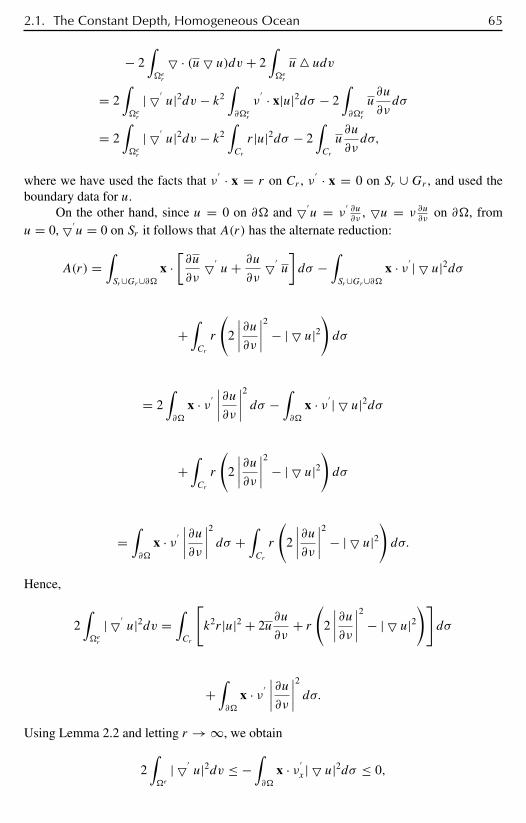
2.1. The Constant Depth, Homogeneous Ocean 65
− 2∫er
· (u u)dv + 2∫er
u udv
= 2∫er
| ′u|2dv − k2
∫∂er
ν′ · x|u|2dσ − 2
∫∂er
u∂u
∂νdσ
= 2∫er
| ′u|2dv − k2
∫Cr
r|u|2dσ − 2∫Cr
u∂u
∂νdσ,
where we have used the facts that ν′ · x = r on Cr , ν
′ · x = 0 on Sr ∪ Gr , and used theboundary data for u.
On the other hand, since u = 0 on ∂ and ′u = ν
′ ∂u∂ν
, u = ν ∂u∂ν
on ∂, fromu = 0, ′
u = 0 on Sr it follows that A(r) has the alternate reduction:
A(r) =∫Sr∪Gr∪∂
x ·[∂u
∂ν′u+ ∂u
∂ν′u
]dσ −
∫Sr∪Gr∪∂
x · ν ′ | u|2dσ
+∫Cr
r
(2
∣∣∣∣∂u∂ν∣∣∣∣2 − | u|2
)dσ
= 2∫∂
x · ν ′∣∣∣∣∂u∂ν
∣∣∣∣2 dσ −∫∂
x · ν ′ | u|2dσ
+∫Cr
r
(2
∣∣∣∣∂u∂ν∣∣∣∣2 − | u|2
)dσ
=∫∂
x · ν ′∣∣∣∣∂u∂ν
∣∣∣∣2 dσ +∫Cr
r
(2
∣∣∣∣∂u∂ν∣∣∣∣2 − | u|2
)dσ.
Hence,
2∫er
| ′u|2dv =
∫Cr
[k2r|u|2 + 2u
∂u
∂ν+ r
(2
∣∣∣∣∂u∂ν∣∣∣∣2 − | u|2
)]dσ
+∫∂
x · ν ′∣∣∣∣∂u∂ν
∣∣∣∣2 dσ.Using Lemma 2.2 and letting r → ∞, we obtain
2∫e
| ′u|2dv ≤ −
∫∂
x · ν ′x | u|2dσ ≤ 0,
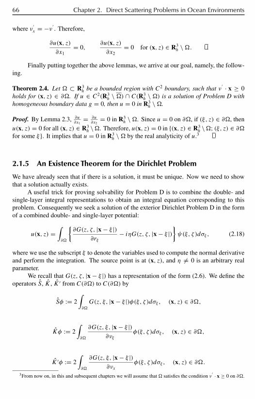
66 Chapter 2. Direct Scattering Problems in Ocean Environments
where ν′x = −ν ′
. Therefore,
∂u(x, z)∂x1
= 0,∂u(x, z)∂x2
= 0 for (x, z) ∈ R3h \.
Finally putting together the above lemmas, we arrive at our goal, namely, the follow-ing.
Theorem 2.4. Let ⊂ R3h be a bounded region with C2 boundary, such that ν
′ · x ≥ 0holds for (x, z) ∈ ∂. If u ∈ C2(R3
h \ ) ∩ C(R3h \ ) is a solution of Problem D with
homogeneous boundary data g = 0, then u = 0 in R3h \.
Proof. By Lemma 2.3, ∂u∂x1
= ∂u∂x2
= 0 in R3h \. Since u = 0 on ∂, if (ξ, z) ∈ ∂, then
u(x, z) = 0 for all (x, z) ∈ R3h \. Therefore, u(x, z) = 0 in (x, z) ∈ R3
h \; (ξ, z) ∈ ∂for some ξ. It implies that u = 0 in R3
h \ by the real analyticity of u.3
2.1.5 An Existence Theorem for the Dirichlet Problem
We have already seen that if there is a solution, it must be unique. Now we need to showthat a solution actually exists.
A useful trick for proving solvability for Problem D is to combine the double- andsingle-layer integral representations to obtain an integral equation corresponding to thisproblem. Consequently we seek a solution of the exterior Dirichlet Problem D in the formof a combined double- and single-layer potential:
u(x, z) =∫∂
∂G(z, ζ, |x − ξ |)
∂rξ− iηG(z, ζ, |x − ξ |)
ψ(ξ, ζ )dσξ , (2.18)
where we use the subscript ξ to denote the variables used to compute the normal derivativeand perform the integration. The source point is at (x, z), and η = 0 is an arbitrary realparameter.
We recall that G(z, ζ, |x − ξ |) has a representation of the form (2.6). We define theoperators S, K , K ′ from C(∂) to C(∂) by
Sφ := 2∫∂
G(z, ξ, |x − ξ |)φ(ξ, ζ )dσξ , (x, z) ∈ ∂,
Kφ := 2∫∂
∂G(z, ξ, |x − ξ |)∂νξ
φ(ξ, ζ )dσξ , (x, z) ∈ ∂,
K ′φ := 2∫∂
∂G(z, ξ, |x − ξ |)∂νx
φ(ξ, ζ )dσξ , (x, z) ∈ ∂.3From now on, in this and subsequent chapters we will assume that satisfies the condition ν
′ · x ≥ 0 on ∂.
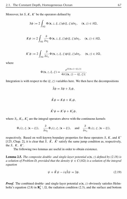
2.1. The Constant Depth, Homogeneous Ocean 67
Moreover, let S, K , K ′ be the operators defined by
Sφ := 2∫∂
(x, z, ξ, ζ )φ(ξ, ζ )dσξ , (x, z) ∈ ∂,
Kφ := 2∫∂
∂
∂νξ(x, z, ξ, ζ )φ(ξ, ζ )dσξ , (x, z) ∈ ∂,
K ′φ := 2∫∂
∂
∂νx(x, z, ξ, ζ )φ(ξ, ζ )dσξ , (x, z) ∈ ∂,
where
(x, z, ξ, ζ ) = eik|(x,z)−(ξ,ζ )|
4π |(x, z)− (ξ, ζ )| .
Integration is with respect to the (ξ, ζ ) variables here. We then have the decompositions
Sφ = Sφ + S1φ,
Kφ = Kφ +K1φ,
K ′φ = K ′φ +K ′1φ,
where S1, K1, K ′1 are the integral operators above with the continuous kernels
1(z, ζ, |x − ξ |), ∂
∂νξ1(z, ζ, |x − ξ |), and
∂
∂νx1(z, ζ, |x − ξ |),
respectively. Based on well-known boundary properties for these operators S, K , and K ′[125, Chap. 2], it is clear that S, K, K ′ satisfy the same jump condition as, respectively,the S, K, K ′.
The following two lemmas are useful in order to obtain existence.
Lemma 2.5. The composite double- and single-layer potential u(x, z) defined by (2.18) isa solution of Problem D, provided that the density ψ ∈ C(∂) is a solution of the integralequation
ψ + Kψ − iηSψ = 2φ. (2.19)
Proof. The combined double- and single-layer potential u(x, z) obviously satisfies Helm-holtz’s equation (2.8) in R3
h \ , the radiation condition (2.3), and the surface and bottom

68 Chapter 2. Direct Scattering Problems in Ocean Environments
conditions (2.2). If (x, z) ∈ R3h \, then by letting (x, z) → (x0, z0) ∈ ∂, we obtain the
integral equation
u(x, z) =∫∂
(∂
∂νξ− iη
)ψdσξ +
∫∂
(∂1
∂νξ− iη1
)ψdσξ
→(
1
2Kψ + ψ − i η
2Sψ
)+(
1
2K1ψ − i η
2S1ψ
)
= 1
2Kψ + ψ − i η
2Sψ.
So if ψ satisfies (2.19), then
lim(x,z)→(x0,z0)
u(x, z) = 1
2Kψ + ψ − i η
2Sψ = φ(x0, z0).
Lemma 2.6. The integral equation (2.19) is uniquely solvable.
Proof. Since K − iηS is a compact operator, we need to prove that the only solution of thehomogeneous form of (2.19) is trivial.
Let ψ ∈ C(∂) be a solution to the homogeneous equation ψ + Kψ − iηSψ = 0,then u as defined by (2.18) solves Problem D with g = 0. Therefore, by the uniquenesstheorem, u = 0 in R3
h \.Let (x, z) ∈ , and define the interior limits as (x0, z0) ∈ ∂,
u− := lim(x,z)→(x0,z0)
u(x, z),∂u−∂νx
:= lim(x,z)→(x0,z0)
∂u(x, z)∂νx
.
From the jump relations we have
−u− = ψ, −∂u−∂νx
= iηψ on ∂.
The first Green’s identity implies that
iη
∫∂
|ψ |2dσ =∫∂
u∂u−∂νx
dσx =∫
(| u|2 − k2|u|2)dvx.
Since k is real, it must follow that ∫∂
|ψ |2dσ = 0
and ψ = 0 on ∂.
Combining Lemmas 2.5 and 2.6, the conclusion then follows.
Theorem 2.7. Problem D is uniquely solvable if x · ν ′ ≥ 0 holds on ∂.
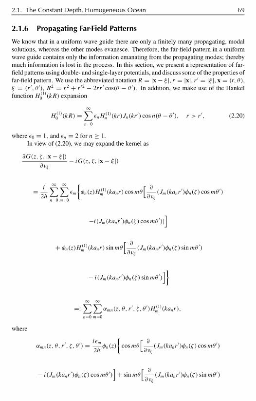
2.1. The Constant Depth, Homogeneous Ocean 69
2.1.6 Propagating Far-Field Patterns
We know that in a uniform wave guide there are only a finitely many propagating, modalsolutions, whereas the other modes evanesce. Therefore, the far-field pattern in a uniformwave guide contains only the information emanating from the propagating modes; therebymuch information is lost in the process. In this section, we present a representation of far-field patterns using double- and single-layer potentials, and discuss some of the properties offar-field pattern. We use the abbreviated notationR = |x − ξ |, r = |x|, r ′ = |ξ |, x = (r, θ),ξ = (r ′, θ ′), R2 = r2 + r ′2 − 2rr ′ cos(θ − θ ′). In addition, we make use of the Hankelfunction H(1)
0 (kR) expansion
H(1)0 (kR) =
∞∑n=0
εnH(1)n (kr)Jn(kr
′) cos n(θ − θ ′), r > r ′, (2.20)
where ε0 = 1, and εn = 2 for n ≥ 1.In view of (2.20), we may expand the kernel as
∂G(z, ζ, |x − ξ |)∂νξ
− iG(z, ζ, |x − ξ |)
= i
2h
∞∑n=0
∞∑m=0
εm
φn(z)H
(1)m (kanr) cosmθ
[ ∂∂νξ
(Jm(kanr′)φn(ζ ) cosmθ ′)
−i(Jm(kanr ′)φn(ζ ) cosmθ ′)|]
+ φn(z)H (1)m (kanr) sinmθ
[ ∂∂νξ
(Jm(kanr′)φn(ζ ) sinmθ ′)
− i(Jm(kanr ′)φn(ζ ) sinmθ ′)]
=:∞∑n=0
∞∑m=0
αmn(z, θ, r′, ζ, θ ′)H (1)
m (kanr),
where
αmn(z, θ, r′, ζ, θ ′) = iεm
2hφn(z)
cosmθ
[ ∂∂νξ
(Jm(kanr′)φn(ζ ) cosmθ ′)
− i(Jm(kanr ′)φn(ζ ) cosmθ ′)]+ sinmθ
[ ∂∂νξ
(Jm(kanr′)φn(ζ ) sinmθ ′)
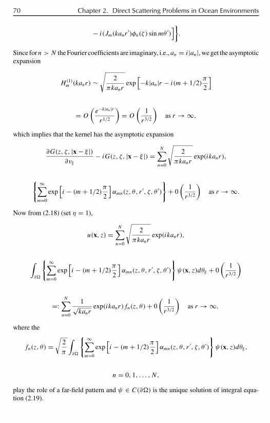
70 Chapter 2. Direct Scattering Problems in Ocean Environments
− i(Jm(kanr ′)φn(ζ ) sinmθ ′)].
Since forn > N the Fourier coefficients are imaginary, i.e., an = i|an|, we get the asymptoticexpansion
H(1)m (kanr) ∼
√2
πkanrexp
[−k|an|r − i(m+ 1/2)
π
2
]
= O
(e−k|an|r
r1/2
)= O
(1
r3/2
)as r → ∞,
which implies that the kernel has the asymptotic expansion
∂G(z, ζ, |x − ξ |)∂νξ
− iG(z, ζ, |x − ξ |) =N∑n=0
√2
πkanrexp(ikanr),
∞∑m=0
exp[i − (m+ 1/2)
π
2
]αmn(z, θ, r
′, ζ, θ ′)
+ 0
(1
r3/2
)as r → ∞.
Now from (2.18) (set η = 1),
u(x, z) =N∑n=0
√2
πkanrexp(ikanr),
∫∂
∞∑m=0
exp[i − (m+ 1/2)
π
2
]αmn(z, θ, r
′, ζ, θ ′)
ψ(x, z)dθξ + 0
(1
r3/2
)
=:N∑n=0
1√kanr
exp(ikanr)fn(z, θ)+ 0
(1
r3/2
)as r → ∞,
where the
fn(z, θ) =√
2
π
∫∂
∞∑m=0
exp[i − (m+ 1/2)
π
2
]αmn(z, θ, r
′, ζ, θ ′)
ψ(x, z)dθξ ,
n = 0, 1, . . . , N,
play the role of a far-field pattern and ψ ∈ C(∂) is the unique solution of integral equa-tion (2.19).
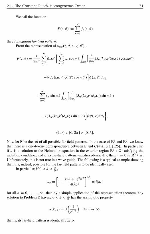
2.1. The Constant Depth, Homogeneous Ocean 71
We call the function
F(z, θ) :=N∑n=0
fn(z, θ)
the propagating far-field pattern.From the representation of αmn(z, θ, r ′, ζ, θ ′),
F(z, θ) = i
2hπ
N∑n=0
φn(z)
∞∑m=0
εm cosmθ∫∂
[ ∂∂νξ
(Jm(kanr′)φn(ζ ) cosmθ ′)
−i(Jm(kanr ′)φn(ζ ) cosmθ ′)]ψ(x, ζ )dσξ
+∞∑m=0
εm sinmθ∫∂
[ ∂∂νξ
(Jm(kanr′)φn(ζ ) sinmθ ′)
−i(Jm(kanr ′)φn(ζ ) sinmθ ′)]ψ(x, ζ )dσξ
,
(θ, z) ∈ [0, 2π ] × [0, h].
Now let F be the set of all possible far-field patterns. In the case of R3 and R2, we knowthat there is a one-to-one correspondence between F and C(∂) (cf. [125]). In particular,if u is a solution to the Helmholtz equation in the exterior region R3 \ satisfying theradiation condition, and if its far-field pattern vanishes identically, then u ≡ 0 in R3 \ .Unfortunately, this is not true in a wave guide. The following is a typical example showingthat it is, indeed, possible for the far-field pattern to be identically zero.
In particular, if 0 < k < π2h ,
an =[
1 − (2h+ 1)2π2
4k2h2
]1/2
= i|an|
for all n = 0, 1, . . . ,∞, then by a simple application of the representation theorem, anysolution to Problem D having 0 < k < π
2h has the asymptotic property
u(x, z) = 0
(1
r3/2
)as r → ∞;
that is, its far-field pattern is identically zero.
72 Chapter 2. Direct Scattering Problems in Ocean Environments
2.1.7 Density Properties of Far-Field Patterns
In this section we discuss scattered waves and the corresponding far-field patterns for agiven incident wave ui . The incident wave ui is scattered by , thereby producing afar-field pattern. We want to extract information about the far field in order to use it toinvestigate the object . A similar problem has already been investigated in R2 by Coltonand Kirsch [123]. They introduced a certain dense subset of the far-field pattern. Coltonand Monk [127], [128] were able to determine the shape of the object by introducing anextremal problem and solving it in projected subspaces. However, in the case of finite depthoceans, we have shown in Gilbert and Xu [211, 210] that the propagating far-field patterncan only carry the information fromN+1 propagating modes, whereN is the largest integerless than 2kh−π
2π . This loss of information makes this nonlinear, improperly posed, inversescattering problem very different from the case studied by Colton and Kirsch [123] and theothers mentioned above.
Let ui be the incident wave and us the corresponding scattered wave. Then, for asound-soft object , the total field u = ui + us satisfies
3u+ k2u = 0 in R3h \, (2.21)
u = 0 as z = 0, (2.22)
∂u
∂z= 0 as z = h, (2.23)
u = 0 on ∂. (2.24)
In addition, the outgoing radiation condition must be satisfied:
limr→∞ r
1/2
(∂usn
∂r− ikanusn
)= 0, r = |x|, n = 0, 1, . . . ,∞, (2.25)
where usn(x) is the nth mode of us .In what follows we consider density properties of the propagating far field in a suitable
subspace of L2(C1), where C1 is the unit cylinder. The decomposition of the propagatingfar field into orthogonal components suggests a numerical algorithm for the express purposeof reconstructing the object .
2.1.8 Complete Sets in L2(∂)
In order to reconstruct an object it is useful to approximate the integral density by a completeset of functions on an arbitrary boundary ∂. The relative complement of in R3
h ise := R3
h \. We use Jn(r) to denote Bessel’s function of order n, and H(1)n (r) to denote
Hankel’s function of the first kind of order n. φn(z) and an are defined as before by (2.4)and (2.5).
2.1. The Constant Depth, Homogeneous Ocean 73
Theorem 2.8. Let λ be a complex number such that 0 ≤ Im λ ≤ ∞ and k = (2n+ 1)π/2hfor n = 0, 1, 2, . . . . Then the sets of functions(
∂
∂ν+ λ
)[φn(z)Jm(kanr) cos(mθ)],(
∂
∂ν+ λ
)[φn(z)Jm(kanr) sin(mθ)],
n,m = 0, 1, . . . ,∞,are complete in L2(∂).
Proof. It suffices to show that if g ∈ L2(∂), if the following projections hold:∫∂
g(r, z, θ)
(∂
∂ν+ λ
)[φn(z)Jm(kanr) cos(mθ)]dσ = 0, (2.26)∫
∂
g(r, z, θ)
(∂
∂ν+ λ
)[φn(z)Jm(kanr) sin(mθ)]dσ = 0 (2.27)
for m, n = 0, 1, . . . ,∞, then g is identically zero on ∂.Let (2.26), (2.27) be true for some g ∈ L2(∂), and let r0 be a solid cylinder
containing in its interior, r0 = (x, z) ∈ R3h, |x| < r0. Then, when (x, z) ∈ R3
h \ r0and (ξ, ζ ) ∈ ∂, we know that for r = |x| > |ξ | = r ′, we can expand the Green’s functionG(z, ζ, |x − ξ |) as
G(z, ζ, |x − ξ |) = i
4
∞∑n=0
∞∑m=0
εmφn(z)φn(ζ )
‖ φn ‖2 H(1)m (kanr)Jm(kanr
′)
× [cos(mθ) cos(mθ ′)+ sin(mθ) sin(mθ ′)]. (2.28)
Here we denote (x, z) in cylindrical coordinates by (r, θ, z) and denote (ξ, ζ ) by (r ′, θ ′, ζ ).From (2.26) and (2.27), we can see that
u(x, z) :=∫∂
(∂
∂νξ+ λ
)G(z, ζ, |x − ξ |)g(r ′, ζ ′, θ ′)dσ (2.29)
is identically zero for (x, z) ∈ R3h \ r0 . Since u, as defined by (2.29), is a solution of
the Helmholtz equation in R3h \r0 , we can conclude by the analyticity of solutions to the
Helmholtz equation [125] that u(x, z) is identically zero for (x,z) ∈ R3h \.
Let (x, z) tend to ∂. Then, in view of the ray representation for the Green’s function(2.13) and from the properties of single- and double-layer potentials, we know (cf. [125],[262]) that
0 = g(x, z)+∫∂
(∂
∂νξ+ λ
)G(z, ζ, |x − ξ |)g(ξ, ζ )dσ, (x, z) ∈ ∂. (2.30)

74 Chapter 2. Direct Scattering Problems in Ocean Environments
Now let us denote by u+(x0, z0), u−(x0, z0) the boundary values
u+(x0, z0) = lim(x,z)→(x0,z0)
u(x, z), (x, z) ∈ e, (x0, z0) ∈ ∂,
and
u−(x0, z0) = lim(x,z)→(x0,z0)
u(x, z), (x, z) ∈ , (x0, z0) ∈ ∂.
Similar definitions are made for ( ∂u∂ν)+ and ( ∂u
∂ν)−. From our knowledge of single- and
double-layer potentials,
u+ − u− = 2g on ∂, (2.31)
and (∂u
∂ν
)+
−(∂u
∂ν
)−
= −2λg on ∂. (2.32)
Since u+ = ( ∂u∂ν)+ = 0, we have from (2.31) and (2.32) that(
∂u
∂ν
)−
+ λu− = 0 on ∂. (2.33)
Hence u, as defined by (2.29), is a solution of the Helmholtz equation in and continuouslyassumes the boundary data (2.33) on ∂. It follows that u ≡ 0 in .
By the relation
g = 1
2(u+ − u−) on ∂,
we can conclude that g = 0 on ∂. This proves Theorem 2.8.
2.1.9 Dense Sets in L2(∂)
In this section we construct a dense set of functions in order to approximate boundary dataon ∂. We modify the notation of [123] to the case of R3
h; namely, let N be the family ofany finite subset of natural numbers containing 0, 1, . . . , N ; C1 = [0, h] × [0, 2π ]; and let
H(k,e) := u : u ∈ C2(e) ∩ C1(e), u satisfies (2.21)–(2.25)
,
A(k, R3h) :=
u : u(x, z) =
∫ 2π
0
∫ h
0g(ζ, θ ′)
∑n∈
φn(ζ )φn(z)eikanx·ydζdθ, (2.34)
where (x, z) ∈ R3h, y = (cos θ ′, sin θ ′), g ∈ L2(C1), ∈ N
. (2.35)
2.1. The Constant Depth, Homogeneous Ocean 75
Moreover, we set
TD(k,e) := u; u = ui + us, ui ∈ A(k,R3
h), us ∈ H(k,e), u = 0 on ∂
,
and
∂TD(k,e)
∂ν
∣∣∣∂
:=∂u
∂ν
∣∣∣∂
: u ∈ TD(k,e).
We want to prove the following theorem.
Theorem 2.9. ∂TD(k,e)
∂ν|∂ is dense in L2(∂).
Proof. Let g ∈ L2(∂) such that∫∂
g∂u
∂νds = 0 for any u ∈ TD(k,e). (2.36)
We need to show that (2.36) implies g = 0 on ∂. If u is an arbitrary element of TD(k,e),then from the representation formula (2.14), we get
u(x, z) = ui(x, z)−∫∂
G(z, ζ, |x − ξ |)∂u∂νdσξ , (2.37)
where ui ∈ A(k,R3h), u = ui + us .
Let (x, z)→ ∂. Then u = 0, and (2.37) implies that
ui(x, z) =∫∂
G(z, ζ, |x − ξ |)∂u∂νdσξ (2.38)
and
∂u(x, z)∂νx
+ 2∫∂
∂
∂νxG(z, ζ, |x − ξ |) ∂u
∂νξdσξ = 2
∂ui(x, z)∂νx
. (2.39)
In view of the representation (2.13) forG(z, ζ, |x−ξ |) and the fact that it is symmetric withrespect to the points (x, z) and (ξ, ζ ), it may be shown that K′ is the adjoint operator to K,subject to the pairing
〈φ,ψ〉 :=∫∂
φψdσ.
Moreover, it can be seen that I + K′ + iS is invertible from section 2.1.5. Now from (2.38)and (2.39) it follows that
(I + K′ + iS)∂u(x, z)∂ν
= 2
(∂ui(x, z)∂ν
+ iui(x, z)), (x, z) ∈ ∂, (2.40)
76 Chapter 2. Direct Scattering Problems in Ocean Environments
and hence
∂u(x, z)∂ν
= 2(I + K′ + iS)−1
(∂ui(x, z)∂ν
+ iui(x, z)), (x, z) ∈ ∂. (2.41)
Substituting (2.41) into (2.36) yields
0 =⟨g,∂u
∂ν
⟩=⟨g, 2(I + K′ + iS)−1
(∂ui
∂ν+ iui
)⟩
= 2
⟨(I + K + iS)−1g,
∂ui
∂ν+ iui
⟩.
Since ui ∈ A(k,R3h), by using the Jacobi–Anger expansion,
φn(z)eikanr cos θ =
∞∑m=−∞
imφn(z)Jm(kanr)eimθ for n = 0, 1, . . . ,∞,
we conclude thatφn(z)Jm(kanr) cos(mθ) andφn(z)Jm(kanr) sin(mθ) are elements ofA(k,R3h).
Hence, from Theorem 2.8, we get
(I + K + iS)−1g = 0
and
g = 0 on ∂.
2.1.10 The Projection Theorem in V N
We will now establish a condition for the far-field patterns to be dense in V N for arbitraryscattering regions which, moreover, satisfy the property x · ν ′ ≥ 0 on ∂. Let N =[ 2kh−π
2π ], where [a] means the integer part of a, and let us introduce the product space
V N := L2[0, 2π ] × spanφ0, φ1, . . . , φN , (2.42)
where the φn, n = 0, 1, . . . , N, are defined by (2.5). From section 2.1.6 we know thatthe propagating far-field patterns from the reduced wave equation, in a homogeneous waveguide, are contained in V N .
We define the injections as follows:(1) P : AN ⊂ A(k,R3
h)→ V N by g := Pu, where
u(x, z) =∫C1
g(θ, ζ )∑n∈
φn(z)φn(ζ )eikanx·ydσ (2.43)
and where g ∈ V N , y = (cos θ ′, sin θ ′), (x, z) ∈ R3h. A
N = u ∈ A(k,R3h) : g ∈ V N).

2.1. The Constant Depth, Homogeneous Ocean 77
(2) F : A(k,R3h) → V N by F(θ, z, k) := Fui , where F(θ, z, k) is the propagating
far-field pattern of us for u = ui + us ∈ TD(k,e).Let ED(k,) = u : u ∈ C2() ∩ C(), u a solution of Helmholtz’s equation in
and u = 0 on ∂.We will prove the following decomposition for the space V N .
Theorem 2.10.
V N = [P(ED(k,) ∩ AN)] ⊕ F(A(k,R3h)),
where F(A(k, R3h)) is the closure of F(A(k, R3
h)) in V N .
Proof. By the representation formula (2.14), we have
us(x, z) =∫∂
(us∂G
∂ν−G∂u
s
∂ν
)dσ, (x, z) ∈ e,
and
0 =∫∂
(ui∂G
∂ν−G∂u
i
∂ν
)dσ, (x, z) ∈ e.
We decompose the total field into the incident and scattered waves, u = ui+us , from whichfollows the integral identity
us(x, z) =∫∂
(u∂G
∂ν−G∂u
∂ν
)dσ, (x, z) ∈ e.
In view of the asymptotic behavior of Hankel’s function and the representation
G(z, ζ, |x − ξ |) = i
2h
∞∑n=0
φn(z)φn(ζ )H(1)0 (kan|x − ξ |),
we obtain the asymptotic formula
us(x, z) = i
2he−iπ/4
N∑n=0
(2
πkanr
)1/2
eikanrfn(θ, z, k)+O(
1
r3/2
), (2.44)
fn(θ, z, k) = φn(z)
∫∂
u(ξ, ζ )
∂
∂νξ(e−ikanx·ξφn(ζ ))− ∂u(ξ, ζ )
∂νξ(e−ikanx·ξφn(ζ ))
dσξ ,
(2.45)
x = (cos θ, sin θ).
The function F(θ, z, k) := ∑Nn=0 fn(θ, z, k) ∈ V N is an alternate representation of
the propagating far-field pattern.

78 Chapter 2. Direct Scattering Problems in Ocean Environments
Let u = ui + us ∈ TD(k,e) and v ∈ ED(k,) ∩ AN , then Pv ∈ V N. From (2.44)and (2.45), we have
us(x, z) = −∫∂
G(z, ζ, |x − ξ |)∂u∂νdσ, (x, z) ∈ e,
Fui(θ, z, k) = −N∑n=0
φn(z)
∫∂
∂u(ξ, ζ )
∂νξ(e−ikanx·ξφn(ζ ))dσξ .
·∫C1
Pv(z, θ)Fui(θ, z, k)dzdθ
= −∫C1
g(z, θ)
[N∑n=0
φn(z)
∫∂
∂u
∂νφn(ζ )e
−ikanx·ξ dσξ
]dzdθ
= −∫∂
∂u
∂νξ
[∫C1
g(z, θ)
N∑n=0
φn(z)e−ikanx·ξ dzdθ
]φn(ζ )dσξ .
Since g(z, θ) ∈ V N , ∫C1
g(z, θ)φn(z)e−ikanx·ξ dzdθ = 0
for any n = N + 1, . . . ,∞, the previous expression becomes∫C1
Pv(z, θ)Fui(θ, z, k)dzdθ = −∫∂
∂u
∂νξv(ξ, ζ )dσξ = 0. (2.46)
This proves the orthogonality
P(ED(k,) ∩ AN) ⊥ F(A(k,R3h)).
Now we prove that
P(ED(k,) ∩ AN) = F(A(k,R3h))
⊥. (2.47)
In fact, if g ∈ V N such that∫C1
g(z, θ)Fui(θ, z, k)dzdθ = 0 ∀ui ∈ A(k,R3h),
then from (2.46) ∫∂
∂u
∂νξv(ξ, ζ )dσξ = 0 ∀u ∈ TD(k,e),
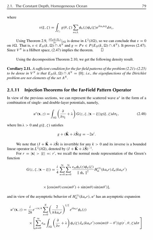
2.1. The Constant Depth, Homogeneous Ocean 79
where
v(ξ, ζ ) =∫C1
g(θ, ζ )∑n∈
φn(z)φn(ζ )eikanx·ydσx.
Using Theorem 2.9, ∂TD(k,e)∂ν
|∂ is dense in L2(∂), so we can conclude that v = 0on ∂. That is, v ∈ ED(k,) ∩ AN and g = Pv ∈ P(ED(k,) ∩ AN). It proves (2.47).Since V N is a Hilbert space, (2.47) implies the theorem.
Using the decomposition Theorem 2.10, we get the following density result.
Corollary 2.11. A sufficient condition for the far-field patterns of the problem (2.21)–(2.25)to be dense in V N is that ED(k,) ∩ AN = 0; i.e., the eigenfunctions of the Dirichletproblem are not elements of the set AN .
2.1.11 Injection Theorems for the Far-Field Pattern Operator
In view of the previous sections, we can represent the scattered wave us in the form of acombination of single- and double-layer potentials, namely,
us(x, z) =∫∂
(∂
∂νξ+ λ
)G(z, ζ, |x − ξ |)g(ξ, ζ )dσξ , (2.48)
where Im λ > 0 and g(ξ, ζ ) satisfies
g + (K + λS)g = −2ui.
We note that (I + K + λS) is invertible for any k > 0 and its inverse is a boundedlinear operator in L2(∂), denoted by (I + K + λS)−1.
For r = |x| > |ξ | =: r ′, we recall the normal mode representation of the Green’sfunction
G(z, ζ, |x − ξ |) = i
4
∞∑n=0
∞∑m=0
εmφn(z)φn(ζ )
‖ φn ‖2 H(1)m (kanr)Jm(kanr
′)
× [cos(mθ) cos(mθ ′)+ sin(mθ) sin(mθ ′)],
and in view of the asymptotic behavior of H(1)m (kanr), u
s has an asymptotic expansion
us(x, z) = i
2he−iπ/4
N∑n=0
(2
πkanr
)1/2
eikanrφn(z)
×[ ∞∑m=0
εm
∫∂
(∂
∂ν+ λ
)φn(ζ )Jm(kanr
′) cos(m(θ − θ ′))g(r′, θ, ζ )dσ
]
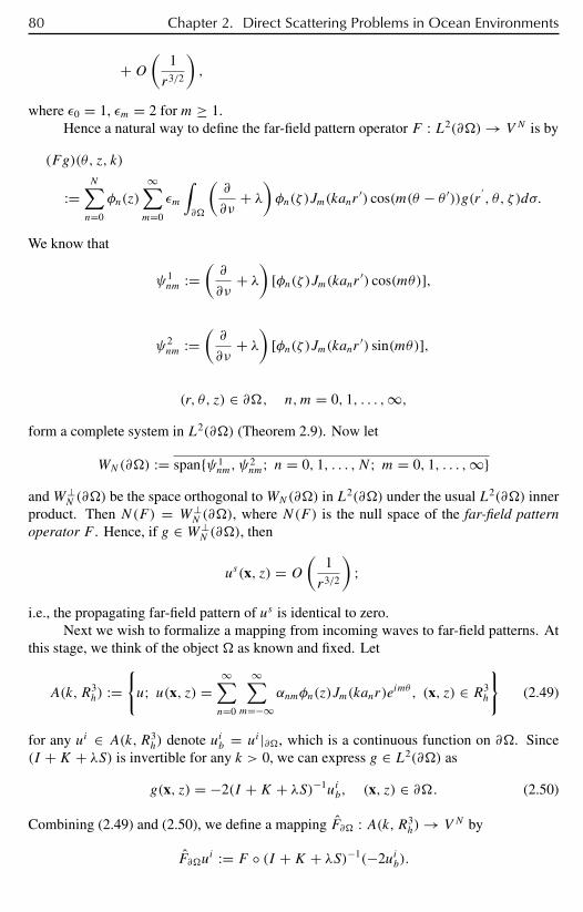
80 Chapter 2. Direct Scattering Problems in Ocean Environments
+O(
1
r3/2
),
where ε0 = 1, εm = 2 for m ≥ 1.Hence a natural way to define the far-field pattern operator F : L2(∂)→ V N is by
(Fg)(θ, z, k)
:=N∑n=0
φn(z)
∞∑m=0
εm
∫∂
(∂
∂ν+ λ
)φn(ζ )Jm(kanr
′) cos(m(θ − θ ′))g(r′, θ, ζ )dσ.
We know that
ψ1nm :=
(∂
∂ν+ λ
)[φn(ζ )Jm(kanr ′) cos(mθ)],
ψ2nm :=
(∂
∂ν+ λ
)[φn(ζ )Jm(kanr ′) sin(mθ)],
(r, θ, z) ∈ ∂, n,m = 0, 1, . . . ,∞,form a complete system in L2(∂) (Theorem 2.9). Now let
WN(∂) := spanψ1nm, ψ
2nm; n = 0, 1, . . . , N; m = 0, 1, . . . ,∞
andW⊥N (∂) be the space orthogonal toWN(∂) in L2(∂) under the usual L2(∂) inner
product. Then N(F) = W⊥N (∂), where N(F) is the null space of the far-field pattern
operator F . Hence, if g ∈ W⊥N (∂), then
us(x, z) = O
(1
r3/2
);
i.e., the propagating far-field pattern of us is identical to zero.Next we wish to formalize a mapping from incoming waves to far-field patterns. At
this stage, we think of the object as known and fixed. Let
A(k,R3h) :=
u; u(x, z) =
∞∑n=0
∞∑m=−∞
αnmφn(z)Jm(kanr)eimθ , (x, z) ∈ R3
h
(2.49)
for any ui ∈ A(k,R3h) denote uib = ui |∂, which is a continuous function on ∂. Since
(I +K + λS) is invertible for any k > 0, we can express g ∈ L2(∂) as
g(x, z) = −2(I +K + λS)−1uib, (x, z) ∈ ∂. (2.50)
Combining (2.49) and (2.50), we define a mapping F∂ : A(k,R3h)→ V N by
F∂ui := F (I +K + λS)−1(−2uib).
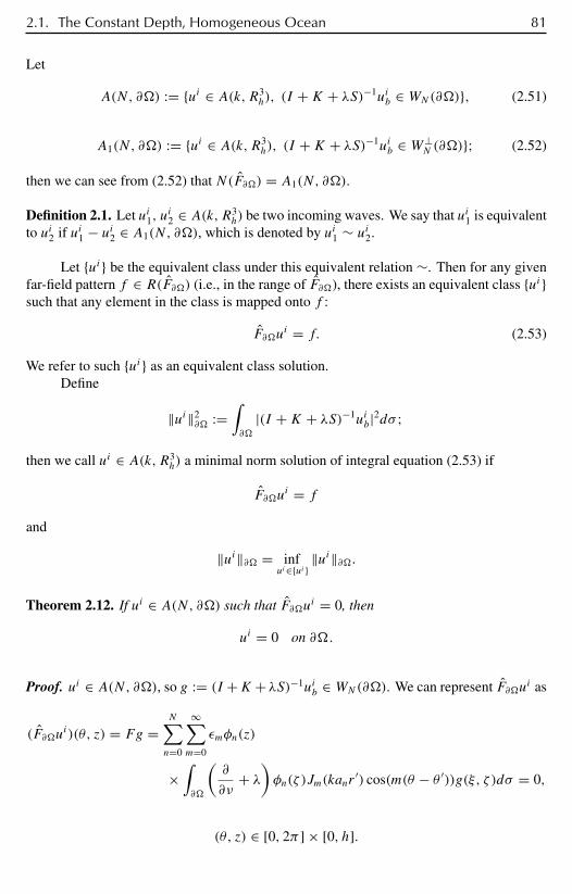
2.1. The Constant Depth, Homogeneous Ocean 81
Let
A(N, ∂) := ui ∈ A(k,R3h), (I +K + λS)−1uib ∈ WN(∂), (2.51)
A1(N, ∂) := ui ∈ A(k,R3h), (I +K + λS)−1uib ∈ W⊥
N (∂); (2.52)
then we can see from (2.52) that N(F∂) = A1(N, ∂).
Definition 2.1. Let ui1, ui2 ∈ A(k,R3
h) be two incoming waves. We say that ui1 is equivalentto ui2 if ui1 − ui2 ∈ A1(N, ∂), which is denoted by ui1 ∼ ui2.
Let ui be the equivalent class under this equivalent relation ∼. Then for any givenfar-field pattern f ∈ R(F∂) (i.e., in the range of F∂), there exists an equivalent class uisuch that any element in the class is mapped onto f :
F∂ui = f. (2.53)
We refer to such ui as an equivalent class solution.Define
‖ui‖2∂ :=
∫∂
|(I +K + λS)−1uib|2dσ ;
then we call ui ∈ A(k,R3h) a minimal norm solution of integral equation (2.53) if
F∂ui = f
and
‖ui‖∂ = infui∈ui
‖ui‖∂.
Theorem 2.12. If ui ∈ A(N, ∂) such that F∂ui = 0, then
ui = 0 on ∂.
Proof. ui ∈ A(N, ∂), so g := (I +K +λS)−1uib ∈ WN(∂). We can represent F∂ui as
(F∂ui)(θ, z) = Fg =
N∑n=0
∞∑m=0
εmφn(z)
×∫∂
(∂
∂ν+ λ
)φn(ζ )Jm(kanr
′) cos(m(θ − θ ′))g(ξ, ζ )dσ = 0,
(θ, z) ∈ [0, 2π ] × [0, h].
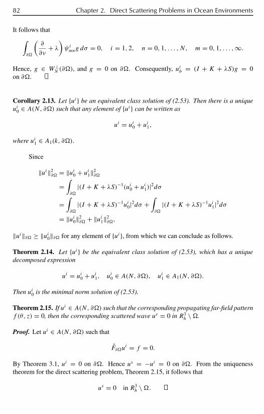
82 Chapter 2. Direct Scattering Problems in Ocean Environments
It follows that∫∂
(∂
∂ν+ λ
)ψimng dσ = 0, i = 1, 2, n = 0, 1, . . . , N, m = 0, 1, . . . ,∞.
Hence, g ∈ W⊥N (∂), and g = 0 on ∂. Consequently, uib = (I + K + λS)g = 0
on ∂.
Corollary 2.13. Let ui be an equivalent class solution of (2.53). Then there is a uniqueui0 ∈ A(N, ∂) such that any element of ui can be written as
ui = ui0 + ui1,
where ui1 ∈ A1(k, ∂).
Since
‖ui‖2∂ = ‖ui0 + ui1‖2
∂
=∫∂
|(I +K + λS)−1(ui0 + ui1)|2dσ
=∫∂
|(I +K + λS)−1ui0|2dσ +∫∂
|(I +K + λS)−1ui1|2dσ= ‖ui0‖2
∂ + ‖ui1‖2∂,
‖ui‖∂ ≥ ‖ui0‖∂ for any element of ui, from which we can conclude as follows.
Theorem 2.14. Let ui be the equivalent class solution of (2.53), which has a uniquedecomposed expression
ui = ui0 + ui1, ui0 ∈ A(N, ∂), ui1 ∈ A1(N, ∂).
Then ui0 is the minimal norm solution of (2.53).
Theorem 2.15. If ui ∈ A(N, ∂) such that the corresponding propagating far-field patternf (θ, z) = 0, then the corresponding scattered wave us = 0 in R3
h \.
Proof. Let ui ∈ A(N, ∂) such that
F∂ui = f = 0.
By Theorem 3.1, ui = 0 on ∂. Hence us = −ui = 0 on ∂. From the uniquenesstheorem for the direct scattering problem, Theorem 2.15, it follows that
us = 0 in R3h \.
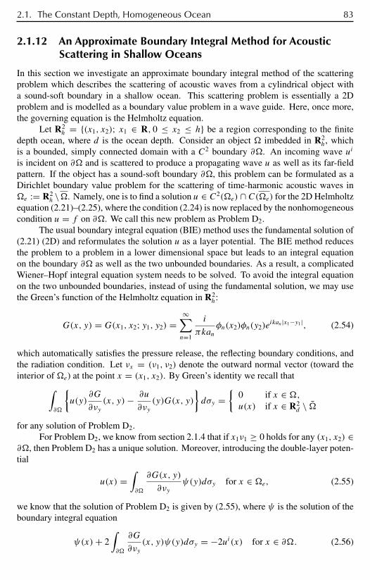
2.1. The Constant Depth, Homogeneous Ocean 83
2.1.12 An Approximate Boundary Integral Method for AcousticScattering in Shallow Oceans
In this section we investigate an approximate boundary integral method of the scatteringproblem which describes the scattering of acoustic waves from a cylindrical object witha sound-soft boundary in a shallow ocean. This scattering problem is essentially a 2Dproblem and is modelled as a boundary value problem in a wave guide. Here, once more,the governing equation is the Helmholtz equation.
Let R2h = (x1, x2); x1 ∈ R, 0 ≤ x2 ≤ h be a region corresponding to the finite
depth ocean, where d is the ocean depth. Consider an object imbedded in R2h, which
is a bounded, simply connected domain with a C2 boundary ∂. An incoming wave ui
is incident on ∂ and is scattered to produce a propagating wave u as well as its far-fieldpattern. If the object has a sound-soft boundary ∂, this problem can be formulated as aDirichlet boundary value problem for the scattering of time-harmonic acoustic waves ine := R2
h \. Namely, one is to find a solution u ∈ C2(e) ∩ C(e) for the 2D Helmholtzequation (2.21)–(2.25), where the condition (2.24) is now replaced by the nonhomogeneouscondition u = f on ∂. We call this new problem as Problem D2.
The usual boundary integral equation (BIE) method uses the fundamental solution of(2.21) (2D) and reformulates the solution u as a layer potential. The BIE method reducesthe problem to a problem in a lower dimensional space but leads to an integral equationon the boundary ∂ as well as the two unbounded boundaries. As a result, a complicatedWiener–Hopf integral equation system needs to be solved. To avoid the integral equationon the two unbounded boundaries, instead of using the fundamental solution, we may usethe Green’s function of the Helmholtz equation in R2
h:
G(x, y) = G(x1, x2; y1, y2) =∞∑n=1
i
πkanφn(x2)φn(y2)e
ikan|x1−y1|, (2.54)
which automatically satisfies the pressure release, the reflecting boundary conditions, andthe radiation condition. Let νx = (ν1, ν2) denote the outward normal vector (toward theinterior of e) at the point x = (x1, x2). By Green’s identity we recall that∫
∂
u(y)
∂G
∂νy(x, y)− ∂u
∂νy(y)G(x, y)
dσy =
0 if x ∈ ,u(x) if x ∈ R2
d \ for any solution of Problem D2.
For Problem D2, we know from section 2.1.4 that if x1ν1 ≥ 0 holds for any (x1, x2) ∈∂, then Problem D2 has a unique solution. Moreover, introducing the double-layer poten-tial
u(x) =∫∂
∂G(x, y)
∂νyψ(y)dσy for x ∈ e, (2.55)
we know that the solution of Problem D2 is given by (2.55), where ψ is the solution of theboundary integral equation
ψ(x)+ 2∫∂
∂G
∂νy(x, y)ψ(y)dσy = −2ui(x) for x ∈ ∂. (2.56)
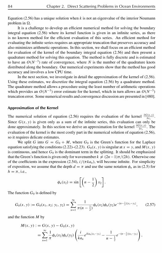
84 Chapter 2. Direct Scattering Problems in Ocean Environments
Equation (2.56) has a unique solution when k is not an eigenvalue of the interior Neumannproblem in .
It is a challenge to develop an efficient numerical method for solving the boundaryintegral equation (2.56) where its kernel function is given in an infinite series, as thereis no known method for the efficient evaluation of this series. An efficient method forevaluating the infinite series requires an appropriate truncation that preserves accuracy andalso minimizes arithmetic operations. In this section, we shall focus on an efficient methodfor evaluation of the kernel of the boundary integral equation (2.56) and then present aquadrature method for solving this equation. The method is fully discrete and is estimatedto have an O(N−3) rate of convergence, where N is the number of the quadrature knotsdistributed along the boundary. Our numerical experiments show that the method has goodaccuracy and involves a low CPU time.
In the next section, we investigate in detail the approximation of the kernel of (2.56).Using these estimates, we discretize the integral equation (2.56) by a quadrature method.The quadrature method allows a procedure using the least number of arithmetic operationswhich provides an O(N−3) error estimate for the kernel, which in turn allows an O(N−3)
truncation error. Some numerical results and convergence discussion are presented in [480].
Approximation of the Kernel
The numerical solution of equation (2.56) requires the evaluation of the kernel ∂G(x,y)
∂νy.
Since G(x, y) is given only as a sum of the infinite series, this evaluation can only bedone approximately. In this section we derive an approximation for the kernel ∂G(x,y)
∂νy. The
evaluation of the kernel is the most costly part in the numerical solution of equation (2.56),so it requires delicate estimates.
We split G into G = G0 + M , where G0 is the Green’s function for the Laplaceequation satisfying the conditions (2.22)–(2.23). G0(x, y) is singular at x = y, andM(x, y)is continuous, and hence G0 is the dominant term in the splitting. It should be emphasizedthat the Green’s function is given only for wavenumber k = (2n−1)π/(2h). Otherwise oneof the coefficients in the expression (2.54), i/(πkan), will become infinite. For simplicityof exposition, we assume that the depth d = π and use the same notation φn as in (2.5) forh = π , i.e.,
φn(x2) = sin
[(n− 1
2
)x2
].
The function G0 is defined by
G0(x, y) := G0(x1, x2; y1, y2) =∞∑n=1
1
π(n− 12 )φn(x2)φn(y2)e
−(n− 12 )|x1−y1|, (2.57)
and the functionM by
M(x, y) : = G(x, y)−G0(x, y)
=∞∑n=1
1
πφn(x2)φn(y2)
(i
kaneikan|x1−y1| − 1
n− 12
e−(n−12 )|x1−y1|
),
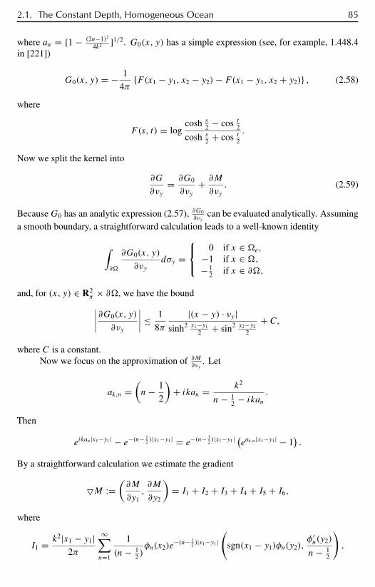
2.1. The Constant Depth, Homogeneous Ocean 85
where an = [1 − (2n−1)2
4k2 ]1/2. G0(x, y) has a simple expression (see, for example, 1.448.4in [221])
G0(x, y) = − 1
4πF(x1 − y1, x2 − y2)− F(x1 − y1, x2 + y2) , (2.58)
where
F(s, t) = logcosh s
2 − cos t2cosh s
2 + cos t2.
Now we split the kernel into
∂G
∂νy= ∂G0
∂νy+ ∂M
∂νy. (2.59)
BecauseG0 has an analytic expression (2.57), ∂G0∂νy
can be evaluated analytically. Assuminga smooth boundary, a straightforward calculation leads to a well-known identity
∫∂
∂G0(x, y)
∂νydσy =
0 if x ∈ e,
−1 if x ∈ ,− 1
2 if x ∈ ∂,
and, for (x, y) ∈ R2π × ∂, we have the bound∣∣∣∣∂G0(x, y)
∂νy
∣∣∣∣ ≤ 1
8π
|(x − y) · νy |sinh2 x1−y1
2 + sin2 x2−y2
2
+ C,
where C is a constant.Now we focus on the approximation of ∂M
∂νy. Let
ak,n =(n− 1
2
)+ ikan = k2
n− 12 − ikan
.
Then
eikan|x1−y1| − e−(n− 12 )|x1−y1| = e−(n−
12 )|x1−y1| (eak,n|x1−y1| − 1
).
By a straightforward calculation we estimate the gradient
M :=(∂M
∂y1,∂M
∂y2
)= I1 + I2 + I3 + I4 + I5 + I6,
where
I1 = k2|x1 − y1|2π
∞∑n=1
1
(n− 12 )φn(x2)e
−(n− 12 )|x1−y1|
(sgn(x1 − y1)φn(y2),
φ′n(y2)
n− 12
),
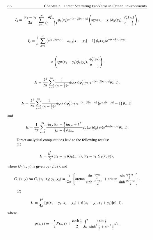
86 Chapter 2. Direct Scattering Problems in Ocean Environments
I2 = |x1 − y1|2π
∞∑n=1
a2k,n
(n− 12 )φn(x2)e
−(n− 12 )|x1−y1|
(sgn(x1 − y1)φn(y2),
φ′n(y2)
n− 12
),
I3 = 1
π
∞∑n=1
(eak,n|x1−y1| − ak,n|x1 − y1| − 1
)φn(x2)e
−(n− 12 )|x1−y1|
×(
sgn(x1 − y1)φn(y2),φ′n(y2)
n− 12
),
I4 = k2
2π
∞∑n=1
1
(n− 12 )
2φn(x2)φ
′n(y2)e
−(n− 12 )|x1−y1|(0, 1),
I5 = k2
2π
∞∑n=1
1
(n− 12 )
2φn(x2)φ
′n(y2)e
−(n− 12 )|x1−y1| (eak,n|x1−y1| − 1
)(0, 1),
and
I6 = 1
2π
∞∑n=1
iak,n[(n− 12 )ak,n + k2]
(n− 12 )
3kanφn(x2)φ
′n(y2)e
ikan|x1−y1|(0, 1).
Direct analytical computations lead to the following results:(1)
I1 = k2
2((x1 − y1)G0(x, y), |x1 − y1|G1(x, y)),
where G0(x, y) is given by (2.58), and
G1(x, y) := G1(x1, x2; y1, y2) = 1
2π
arctan
sin x2−y2
2
sinh |x1−y1|2
+ arctansin x2+y2
2
sinh |x1−y1|2
.
(2)
I4 = k2
4π[φ(x1 − y1, x2 − y2)+ φ(x1 − y1, x2 + y2)](0, 1),
where
φ(s, t) = − t2F(s, t)+ cosh s
2
2
∫ t
0
z sin z2
sinh2 s2 + sin2 z
2
dz.
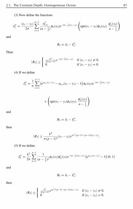
2.1. The Constant Depth, Homogeneous Ocean 87
(3) Now define the functions
Ip
2 = |x1 − y1|2π
p−1∑n=1
a2k,n
(n− 12 )φn(x2)e
−(n− 12 )|x1−y1|
(sgn(x1 − y1)φn(y2),
φ′n(y2)
n− 12
)
and
R2 = I2 − Ip2 .Then
|R2| ≤
k4
2π(p−1)3 e−(p−1)|x1−y1| if |x1 − y1| = 0,
0 if |x1 − y1| = 0.
(4) If we define
Ip
3 = 1
π
p−1∑n=1
(eak,n|x1−y1| − ak,n|x1 − y1| − 1
)φn(x2)e
−(n− 12 )|x1−y1|
×(
sgn(x1 − y1)φn(y2),φ′n(y2)
n− 12
)
and
R3 = I3 − Ip3 ,then
|R3| ≤ k4
π(p − 1)2|x1 − y1|e(κ2/(p−1)−(p−1))|x1−y1|.
(5) If we define
Ip
5 = k2
2π
p−1∑n=1
1
(n− 12 )
2φn(x2)φ
′n(y2)e
−(n− 12 )|x1−y1| (eak,n|x1−y1| − 1
)(0, 1)
and
R5 = I5 − Ip5 ,then
|R5| ≤
k4
π(p−1)3 e(κ2/(p−1)−(p−1))|x1−y1| if |x1 − y1| = 0,
0 if |x1 − y1| = 0.
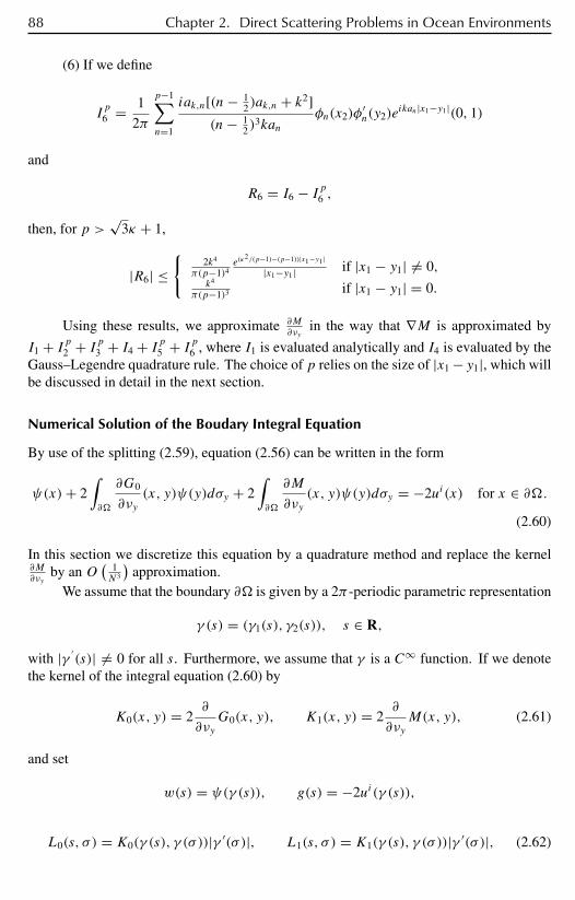
88 Chapter 2. Direct Scattering Problems in Ocean Environments
(6) If we define
Ip
6 = 1
2π
p−1∑n=1
iak,n[(n− 12 )ak,n + k2]
(n− 12 )
3kanφn(x2)φ
′n(y2)e
ikan|x1−y1|(0, 1)
and
R6 = I6 − Ip6 ,
then, for p >√
3κ + 1,
|R6| ≤
2k4
π(p−1)4e(κ
2/(p−1)−(p−1))|x1−y1 ||x1−y1| if |x1 − y1| = 0,
k4
π(p−1)3 if |x1 − y1| = 0.
Using these results, we approximate ∂M∂νy
in the way that ∇M is approximated by
I1 + Ip2 + Ip3 + I4 + Ip5 + Ip6 , where I1 is evaluated analytically and I4 is evaluated by theGauss–Legendre quadrature rule. The choice of p relies on the size of |x1 − y1|, which willbe discussed in detail in the next section.
Numerical Solution of the Boudary Integral Equation
By use of the splitting (2.59), equation (2.56) can be written in the form
ψ(x)+ 2∫∂
∂G0
∂νy(x, y)ψ(y)dσy + 2
∫∂
∂M
∂νy(x, y)ψ(y)dσy = −2ui(x) for x ∈ ∂.
(2.60)
In this section we discretize this equation by a quadrature method and replace the kernel∂M∂νy
by an O(
1N3
)approximation.
We assume that the boundary ∂ is given by a 2π -periodic parametric representation
γ (s) = (γ1(s), γ2(s)), s ∈ R,
with |γ ′(s)| = 0 for all s. Furthermore, we assume that γ is a C∞ function. If we denote
the kernel of the integral equation (2.60) by
K0(x, y) = 2∂
∂νyG0(x, y), K1(x, y) = 2
∂
∂νyM(x, y), (2.61)
and set
w(s) = ψ(γ (s)), g(s) = −2ui(γ (s)),
L0(s, σ ) = K0(γ (s), γ (σ ))|γ ′(σ )|, L1(s, σ ) = K1(γ (s), γ (σ ))|γ ′(σ )|, (2.62)
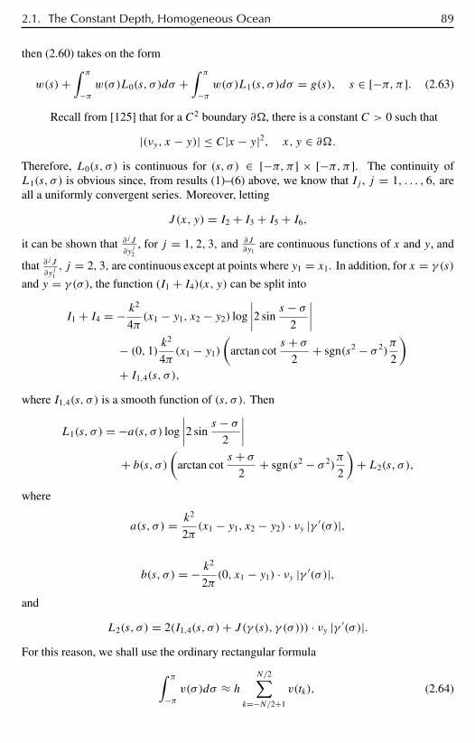
2.1. The Constant Depth, Homogeneous Ocean 89
then (2.60) takes on the form
w(s)+∫ π
−πw(σ)L0(s, σ )dσ +
∫ π
−πw(σ)L1(s, σ )dσ = g(s), s ∈ [−π, π ]. (2.63)
Recall from [125] that for a C2 boundary ∂, there is a constant C > 0 such that
|(νy, x − y)| ≤ C|x − y|2, x, y ∈ ∂.Therefore, L0(s, σ ) is continuous for (s, σ ) ∈ [−π, π ] × [−π, π ]. The continuity ofL1(s, σ ) is obvious since, from results (1)–(6) above, we know that Ij , j = 1, . . . , 6, areall a uniformly convergent series. Moreover, letting
J (x, y) = I2 + I3 + I5 + I6,
it can be shown that ∂j J
∂yj
2
, for j = 1, 2, 3, and ∂J∂y1
are continuous functions of x and y, and
that ∂j J
∂yj
1
, j = 2, 3, are continuous except at points where y1 = x1. In addition, for x = γ (s)
and y = γ (σ ), the function (I1 + I4)(x, y) can be split into
I1 + I4 = − k2
4π(x1 − y1, x2 − y2) log
∣∣∣∣2 sins − σ
2
∣∣∣∣− (0, 1) k
2
4π(x1 − y1)
(arctan cot
s + σ2
+ sgn(s2 − σ 2)π
2
)+ I1,4(s, σ ),
where I1,4(s, σ ) is a smooth function of (s, σ ). Then
L1(s, σ ) = −a(s, σ ) log
∣∣∣∣2 sins − σ
2
∣∣∣∣+ b(s, σ )
(arctan cot
s + σ2
+ sgn(s2 − σ 2)π
2
)+ L2(s, σ ),
where
a(s, σ ) = k2
2π(x1 − y1, x2 − y2) · νy |γ ′(σ )|,
b(s, σ ) = − k2
2π(0, x1 − y1) · νy |γ ′(σ )|,
and
L2(s, σ ) = 2(I1,4(s, σ )+ J (γ (s), γ (σ ))) · νy |γ ′(σ )|.For this reason, we shall use the ordinary rectangular formula∫ π
−πv(σ )dσ ≈ h
N/2∑k=−N/2+1
v(tk), (2.64)
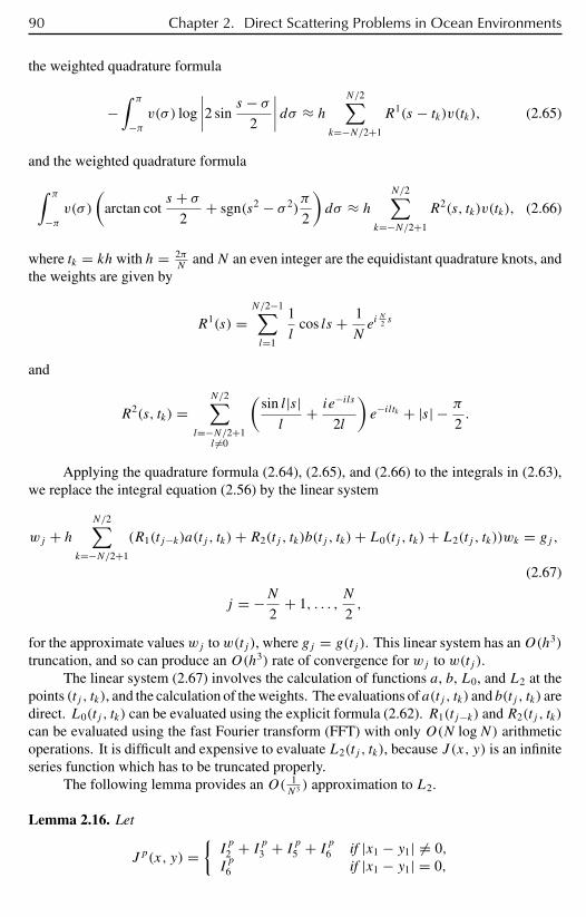
90 Chapter 2. Direct Scattering Problems in Ocean Environments
the weighted quadrature formula
−∫ π
−πv(σ ) log
∣∣∣∣2 sins − σ
2
∣∣∣∣ dσ ≈ h
N/2∑k=−N/2+1
R1(s − tk)v(tk), (2.65)
and the weighted quadrature formula∫ π
−πv(σ )
(arctan cot
s + σ2
+ sgn(s2 − σ 2)π
2
)dσ ≈ h
N/2∑k=−N/2+1
R2(s, tk)v(tk), (2.66)
where tk = khwith h = 2πN
andN an even integer are the equidistant quadrature knots, andthe weights are given by
R1(s) =N/2−1∑l=1
1
lcos ls + 1
Nei
N2 s
and
R2(s, tk) =N/2∑
l=−N/2+1l =0
(sin l|s|l
+ ie−ils
2l
)e−iltk + |s| − π
2.
Applying the quadrature formula (2.64), (2.65), and (2.66) to the integrals in (2.63),we replace the integral equation (2.56) by the linear system
wj + hN/2∑
k=−N/2+1
(R1(tj−k)a(tj , tk)+ R2(tj , tk)b(tj , tk)+ L0(tj , tk)+ L2(tj , tk))wk = gj ,
(2.67)
j = −N2
+ 1, . . . ,N
2,
for the approximate valueswj tow(tj ), where gj = g(tj ). This linear system has anO(h3)
truncation, and so can produce an O(h3) rate of convergence for wj to w(tj ).The linear system (2.67) involves the calculation of functions a, b, L0, and L2 at the
points (tj , tk), and the calculation of the weights. The evaluations of a(tj , tk) and b(tj , tk) aredirect. L0(tj , tk) can be evaluated using the explicit formula (2.62). R1(tj−k) and R2(tj , tk)
can be evaluated using the fast Fourier transform (FFT) with only O(N logN) arithmeticoperations. It is difficult and expensive to evaluate L2(tj , tk), because J (x, y) is an infiniteseries function which has to be truncated properly.
The following lemma provides an O( 1N3 ) approximation to L2.
Lemma 2.16. Let
Jp(x, y) =Ip
2 + Ip3 + Ip5 + Ip6 if |x1 − y1| = 0,Ip
6 if |x1 − y1| = 0,
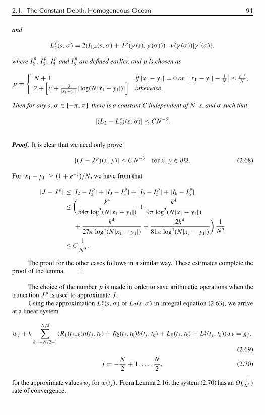
2.1. The Constant Depth, Homogeneous Ocean 91
and
L∗2(s, σ ) = 2(I1,4(s, σ )+ Jp(γ (s), γ (σ ))) · ν(γ (σ ))|γ ′(σ )|,
where Ip2 , Ip
3 , Ip
5 and Ip6 are defined earlier, and p is chosen as
p =N + 1 if |x1 − y1| = 0 or
∣∣|x1 − y1| − 1N
∣∣ ≤ e−1
N,
2 +[κ + 3
|x1−y1| | log(N |x1 − y1|)|]
otherwise.
Then for any s, σ ∈ [−π, π ], there is a constant C independent of N , s, and σ such that
|(L2 − L∗2)(s, σ )| ≤ CN−3.
Proof. It is clear that we need only prove
|(J − Jp)(x, y)| ≤ CN−3 for x, y ∈ ∂. (2.68)
For |x1 − y1| ≥ (1 + e−1)/N , we have from that
|J − Jp| ≤ |I2 − Ip2 | + |I3 − Ip3 | + |I5 − Ip5 | + |I6 − Ip6 |≤(
k4
54π log3(N |x1 − y1|)+ k4
9π log2(N |x1 − y1|)+ k4
27π log3(N |x1 − y1|)+ 2k4
81π log4(N |x1 − y1|))
1
N3
≤ C 1
N3.
The proof for the other cases follows in a similar way. These estimates complete theproof of the lemma.
The choice of the number p is made in order to save arithmetic operations when thetruncation Jp is used to approximate J .
Using the approximation L∗2(s, σ ) of L2(s, σ ) in integral equation (2.63), we arrive
at a linear system
wj + hN/2∑
k=−N/2+1
(R1(tj−k)a(tj , tk)+ R2(tj , tk)b(tj , tk)+ L0(tj , tk)+ L∗2(tj , tk))wk = gj ,
(2.69)
j = −N2
+ 1, . . . ,N
2, (2.70)
for the approximate valueswj forw(tj ). From Lemma 2.16, the system (2.70) has anO( 1N3 )
rate of convergence.
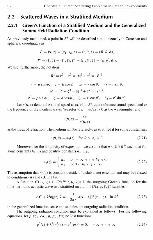
92 Chapter 2. Direct Scattering Problems in Ocean Environments
2.2 Scattered Waves in a Stratified Medium
2.2.1 Green’s Function of a Stratified Medium and the GeneralizedSommerfeld Radiation Condition
As previously mentioned, a point in R3 will be described simultaneously in Cartesian andspherical coordinates as
P = (x, z) = (x1, x2, z) = (r, θ, z) = (R, θ, φ),
P ′ = (ξ, ζ ) = (ξ1, ξ2, ζ ) = (r′, θ
′, ζ ) = (ρ, θ
′, φ
′).
We use, furthermore, the notation
R2 = r2 + z2 = |x|2 + z2 = |P |2,r = R sin φ, z = R cosφ, x1 = r cos θ, x2 = r sin θ,
ρ2 = r′2 + ζ 2 = |ξ |2 + ζ 2 = |P ′|2,
r′ = ρ sin φ
′, ζ = ρ cosφ
′, ξ1 = r ′ cos θ ′, ξ2 = r ′ sin θ ′.
Let c(x, z) denote the sound speed at (x, z) ∈ R3, c0 a reference sound speed, and ωthe frequency of the incident wave. We refer to k = ω/c0 > 0 as the wavenumber and
n(x, z) = c0
c(x, z)
as the index of refraction. The medium will be referred to as stratified if for some constant a0,
n(x, z) = n0(z) for R > a0 > 0. (2.71)
Moreover, for the simplicity of exposition, we assume that n ∈ C1(R3) such that forsome constants h1, h2 and positive constants n−, n+,
n0(z) =n− for − ∞ < z < h1 < 0,n+ for 0 < h2 < z <∞. (2.72)
The assumption that n0(z) is constant outside of a slab is not essential and may be relaxedto conditions (A) and (B) in [470].
A function G(·; ξ, ζ ) ∈ C2(R3 \ (ξ, ζ )) is the outgoing Green’s function for thetime-harmonic acoustic wave in a stratified medium if G(x, z; ξ, ζ ) satisfies
G+ k2n20(z)G = − 1
2πrδ(|x − ξ |)δ(z− ζ ) in R3 (2.73)
in the generalized function sense and satisfies the outgoing radiation condition.The outgoing radiation condition may be explained as follows. For the following
equations, let p1(z<, ka), p2(z>, ka) be Jost functions:
p′′(z)+ k2[n2
0(z)− a2]p(z) = 0, −∞ < z <∞; (2.74)
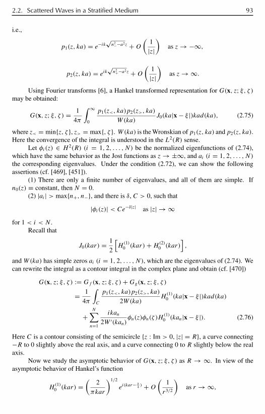
2.2. Scattered Waves in a Stratified Medium 93
i.e.,
p1(z, ka) = e−ik√n2−−a2z +O
(1
|z|)
as z → −∞,
p2(z, ka) = eik√n2+−a2z +O
(1
|z|)
as z → ∞.
Using Fourier transforms [6], a Hankel transformed representation for G(x, z; ξ, ζ )may be obtained:
G(x, z; ξ, ζ ) = 1
4π
∫ ∞
0
p1(z<, ka)p2(z>, ka)
W(ka)J0(ka|x − ξ |)kad(ka), (2.75)
where z< = minz, ζ , z> = max, ζ . W(ka) is the Wronskian of p1(z, ka) andp2(z, ka).Here the convergence of the integral is understood in the L2(R) sense.
Let φi(z) ∈ H 2(R) (i = 1, 2, . . . , N) be the normalized eigenfunctions of (2.74),which have the same behavior as the Jost functions as z → ±∞, and ai (i = 1, 2, . . . , N)the corresponding eigenvalues. Under the condition (2.72), we can show the followingassertions (cf. [469], [451]).
(1) There are only a finite number of eigenvalues, and all of them are simple. Ifn0(z) ≡ constant, then N = 0.
(2) |ai | > maxn+, n−, and there is δ, C > 0, such that
|φi(z)| < Ce−δ|z| as |z| → ∞for 1 < i < N .
Recall that
J0(kar) = 1
2
[H(1)0 (kar)+H(2)
0 (kar)],
andW(ka) has simple zeros ai (i = 1, 2, . . . , N), which are the eigenvalues of (2.74). Wecan rewrite the integral as a contour integral in the complex plane and obtain (cf. [470])
G(x, z; ξ, ζ ) := Gf (x, z; ξ, ζ )+Gg(x, z; ξ, ζ )= 1
4π
∫C
p1(z<, ka)p2(z>, ka)
2W(ka)H(1)0 (ka|x − ξ |)kad(ka)
+N∑n=1
ikan
2W ′(kan)φn(z)φn(ζ )H
(1)0 (kan|x − ξ |). (2.76)
Here C is a contour consisting of the semicircle z : Im > 0, |z| = R, a curve connecting−R to 0 slightly above the real axis, and a curve connecting 0 to R slightly below the realaxis.
Now we study the asymptotic behavior of G(x, z; ξ, ζ ) as R → ∞. In view of theasymptotic behavior of Hankel’s function
H(1)0 (kar) =
(2
πkar
)1/2
ei(kar−π4 ) +O
(1
r3/2
)as r → ∞,
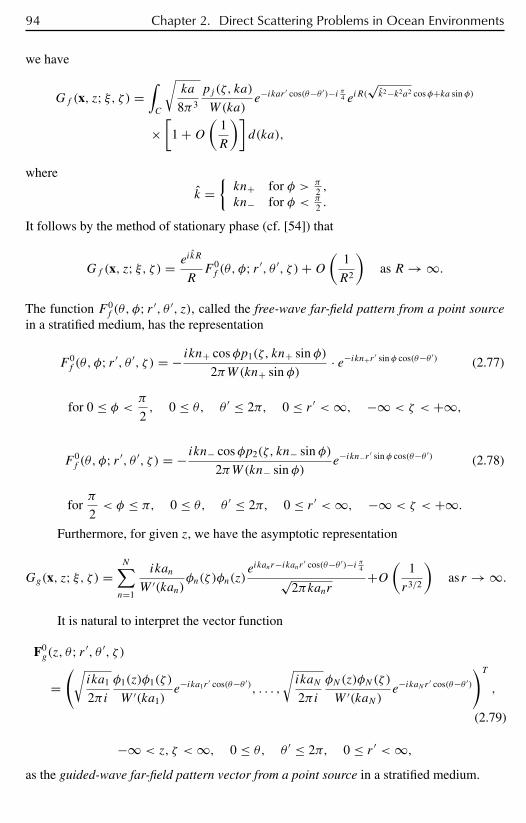
94 Chapter 2. Direct Scattering Problems in Ocean Environments
we have
Gf (x, z; ξ, ζ ) =∫C
√ka
8π3
pj (ζ, ka)
W(ka)e−ikar
′ cos(θ−θ ′)−i π4 eiR(√k2−k2a2 cosφ+ka sin φ)
×[
1 +O(
1
R
)]d(ka),
where
k =kn+ for φ > π
2 ,
kn− for φ < π2 .
It follows by the method of stationary phase (cf. [54]) that
Gf (x, z; ξ, ζ ) = eikR
RF 0f (θ, φ; r ′, θ ′, ζ )+O
(1
R2
)as R → ∞.
The function F 0f (θ, φ; r ′, θ ′, z), called the free-wave far-field pattern from a point source
in a stratified medium, has the representation
F 0f (θ, φ; r ′, θ ′, ζ ) = − ikn+ cosφp1(ζ, kn+ sin φ)
2πW(kn+ sin φ)· e−ikn+r ′ sin φ cos(θ−θ ′) (2.77)
for 0 ≤ φ < π
2, 0 ≤ θ, θ ′ ≤ 2π, 0 ≤ r ′ <∞, −∞ < ζ < +∞,
F 0f (θ, φ; r ′, θ ′, ζ ) = − ikn− cosφp2(ζ, kn− sin φ)
2πW(kn− sin φ)e−ikn−r ′ sin φ cos(θ−θ ′) (2.78)
forπ
2< φ ≤ π, 0 ≤ θ, θ ′ ≤ 2π, 0 ≤ r ′ <∞, −∞ < ζ < +∞.
Furthermore, for given z, we have the asymptotic representation
Gg(x, z; ξ, ζ ) =N∑n=1
ikan
W ′(kan)φn(ζ )φn(z)
eikanr−ikanr ′ cos(θ−θ ′)−i π4√2πkanr
+O(
1
r3/2
)as r → ∞.
It is natural to interpret the vector function
F0g(z, θ; r ′, θ ′, ζ )
=(√
ika1
2πi
φ1(z)φ1(ζ )
W ′(ka1)e−ika1r
′ cos(θ−θ ′), . . . ,
√ikaN
2πi
φN(z)φN(ζ )
W ′(kaN)e−ikaN r
′ cos(θ−θ ′)
)T,
(2.79)
−∞ < z, ζ <∞, 0 ≤ θ, θ ′ ≤ 2π, 0 ≤ r ′ <∞,as the guided-wave far-field pattern vector from a point source in a stratified medium.
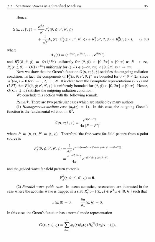
2.2. Scattered Waves in a Stratified Medium 95
Hence,
G(x, z; ξ, ζ ) = eikR
RF 0f (θ, φ; r ′, θ ′, ζ )
+ 1√r
Ag(r) · F0g(z, θ, r
′, θ ′, ζ )+ R0f (R, θ, φ)+ R0
g(r, z, θ), (2.80)
whereAg(r) = (eika1r , eika2r , . . . , eikaN r )
and R0f (R, θ, φ) = O(1/R2) uniformly for (θ, φ) ∈ [0, 2π ] × [0, π ] as R → ∞,
R0g(r, z, θ) = O(1/r3/2) uniformly for (z, θ) ∈ (−∞,∞)× [0, 2π ] as r → ∞.
Now we show that the Green’s function G(x, z; ξ, ζ ) satisfies the outgoing radiationcondition. In fact, the components of F0
g(z, θ; r ′, θ, ζ ) are bounded for 0 ≤ θ ≤ 2π sinceW ′(kai) = 0 for i = 1, 2, . . . , N . It is clear from the asymptotic representations (2.77) and(2.87) that F 0
f (θ, φ; r ′, θ ′, ζ ) is uniformly bounded for (θ, φ) ∈ [0, 2π ] × [0, π ]. Hence,G(x, z; ξ, ζ ) satisfies the outgoing radiation condition.
We conclude this section with the following remark.
Remark. There are two particular cases which are studied by many authors.(1) Homogeneous medium case (n0(z) ≡ 1). In this case, the outgoing Green’s
function is the fundamental solution in R3,
G(x, z; ξ, ζ ) = eik|P−P ′|
4π |P − P ′| ,
where P = (x, z), P ′ = (ξ, ζ ). Therefore, the free-wave far-field pattern from a pointsource is
F 0f (θ, φ; r ′, θ ′, ζ ) = 1
4πe−ikρ[cosφ cosφ′+sin φ sin φ′ cos(θ−θ ′)]
= e−ikζ cosφ
4πe−ikr
′ sin φ cos(θ−θ ′),
and the guided-wave far-field pattern vector is
F0g(z, θ; r ′, θ ′, ζ ) = 0.
(2) Parallel wave guide case. In ocean acoustics, researchers are interested in thecase where the acoustic wave is trapped in a slab R3
h := (x, z) ∈ R3|z ∈ [0, h] such that
u(x, 0) = 0,∂u
∂z(x, h) = 0.
In this case, the Green’s function has a normal mode representation
G(x, z; ξ, ζ ) =∞∑n=1
φn(z)φn(ζ )H(1)0 (kan|x − ξ |),

96 Chapter 2. Direct Scattering Problems in Ocean Environments
where φn(z) and an are, respectively, the nth eigenfunction and eigenvalue of the Sturm–Liouville system
φ′′(z)+ k2[n20(z)− a2]φ(z) = 0, 0 < z < h.
φ(0) = 0, φ′(h) = 0.
Hence, the free-wave far-field pattern is identical to zero, as we expected. The guided-wavefar-field pattern is given by(
φ1(z)φ1(ζ )√ka1πi
e−ika1r′ cos(θ−θ ′), . . . ,
φN(z)φN(ζ )√kaNπi
e−ikaN r′ cos(θ−θ ′)
).
Here N is the number of the propagating modes. From (2.77), (2.78), and (2.79) we havethe following lemmas.
Lemma 2.17. For given α ∈ S1, F 0f (α;P ′) is a solution to the corresponding homogeneous
form of (2.73) with respect to P ′ ∈ R3.For given (x, z) ∈ D1, each component of F0
g(x, z;P ′) is a solution to the corre-sponding homogeneous form of (2.73) with respect to P ′ ∈ R3.
Lemma 2.18. For any given P ′ ∈ R3, z ∈ R, F 0g (θ, z;P ′; j) (0 ≤ j ≤ N) are analytic4
in θ for θ ∈ [0, 2π ]. For any given P ′ ∈ R3, F 0f (θ, φ, P
′) is analytic in θ and φ forθ ∈ [0, 2π ] and φ ∈ [0, π/2) ∪ (π/2, π ].
In what follows we prove three reciprocity relations among the free-wave far-fieldpatterns and the guided-wave far-field pattern vectors corresponding to incident distortedplane waves and normal mode waves. Then we prove conditions under which a set offar-field patterns is complete in a Hilbert space based on the reciprocity relation. Theseproperties are important in investigating the inverse scattering problems.
2.2.2 Scattering of Acoustic Waves by an Obstacle in a StratifiedSpace
In a stratified medium, sound waves may be trapped by acoustic ducts and caused to prop-agate horizontally [470], [54], [451], [446]. In this case, the waves scattered by either acompact obstacle or a local inhomogeneity does not, in general, satisfy the Sommerfeldradiation condition, but rather a generalized Sommerfeld condition. Consequently, we referto these scattering problems as generalized scattering problems.
In this section, we investigate the scattering of time-harmonic, acoustic waves in astratified medium with a local inhomogeneity. The uniqueness and existence of the gener-alized, direct scattering problem is established using integral equation methods. Relationsbetween the far field of scattered acoustic waves and the sound profile of the inhomogeneitywill be obtained. Using these relations, we shall prove three reciprocity relations amongthe free-wave far-field patterns and the guided-wave far-field pattern vectors corresponding
4By analytic here we mean that the real and imaginary parts are real analytic functions.

2.2. Scattered Waves in a Stratified Medium 97
to incident distorted plane waves and normal modes. Then, based on these reciprocity rela-tions, we shall establish a condition under which a set of far-field patterns forms a completesubspace of a Hilbert space. These properties are important for investigating generalized,inverse scattering problems.
Let be a bounded domain with C2 boundary. The obstacle, scattering problemsfor a time-harmonic wave can be described mathematically as follows: Given an incidentwave, ui ∈ C2(R3), satisfying
ui + k2n20(z)u
i = 0 in R3, (2.81)
find the scattered field us ∈ C2(R3 \ ),us + k2n2
0(z)us = 0 in R3 \, (2.82)
such that the total field, u = ui + us, satisfies one of the following boundary conditionsdepending on the physical property of the obstacle.
(1) Dirichlet condition (Problem D):
u = 0 on ∂. (2.83)
(2) Neumann condition (Problem N):
∂u
∂ν= 0 on ∂. (2.84)
(3) Robin condition (Problem R):
∂u
∂ν+ σu = 0 on ∂, (2.85)
where σ ∈ C(∂) and σ > 0.Moreover, the scattered wave us(x, z) satisfies the generalized outgoing radiation
condition. That is, we define the scattered guided wave usg and the scattered free wave usfas follows:
un(x) =∫ ∞
−∞φn(ζ )u
s(x, z)dζ,
usg(x, z) =N∑n=1
φn(z)un(x),
usf (x, z) = us(x, z)− usg(x, z);however, usf and un satisfy
∂usf
∂R− ikusf = O
(1
R2
), usf = O
(1
R
),
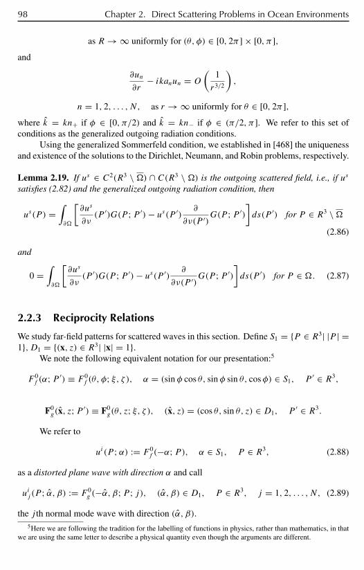
98 Chapter 2. Direct Scattering Problems in Ocean Environments
as R → ∞ uniformly for (θ, φ) ∈ [0, 2π ] × [0, π ],and
∂un
∂r− ikanun = O
(1
r3/2
),
n = 1, 2, . . . , N, as r → ∞ uniformly for θ ∈ [0, 2π ],where k = kn+ if φ ∈ [0, π/2) and k = kn− if φ ∈ (π/2, π ]. We refer to this set ofconditions as the generalized outgoing radiation conditions.
Using the generalized Sommerfeld condition, we established in [468] the uniquenessand existence of the solutions to the Dirichlet, Neumann, and Robin problems, respectively.
Lemma 2.19. If us ∈ C2(R3 \ ) ∩ C(R3 \ ) is the outgoing scattered field, i.e., if us
satisfies (2.82) and the generalized outgoing radiation condition, then
us(P ) =∫∂
[∂us
∂ν(P ′)G(P ;P ′)− us(P ′)
∂
∂ν(P ′)G(P ;P ′)
]ds(P ′) for P ∈ R3 \
(2.86)
and
0 =∫∂
[∂us
∂ν(P ′)G(P ;P ′)− us(P ′)
∂
∂ν(P ′)G(P ;P ′)
]ds(P ′) for P ∈ . (2.87)
2.2.3 Reciprocity Relations
We study far-field patterns for scattered waves in this section. Define S1 = P ∈ R3| |P | =1,D1 = (x, z) ∈ R3| |x| = 1.
We note the following equivalent notation for our presentation:5
F 0f (α;P ′) ≡ F 0
f (θ, φ; ξ, ζ ), α = (sin φ cos θ, sin φ sin θ, cosφ) ∈ S1, P ′ ∈ R3,
F0g(x, z;P ′) ≡ F0
g(θ, z; ξ, ζ ), (x, z) = (cos θ, sin θ, z) ∈ D1, P ′ ∈ R3.
We refer to
ui(P ;α) := F 0f (−α;P), α ∈ S1, P ∈ R3, (2.88)
as a distorted plane wave with direction α and call
uij (P ; α, β) := F 0g (−α, β;P ; j), (α, β) ∈ D1, P ∈ R3, j = 1, 2, . . . , N, (2.89)
the j th normal mode wave with direction (α, β).5Here we are following the tradition for the labelling of functions in physics, rather than mathematics, in that
we are using the same letter to describe a physical quantity even though the arguments are different.
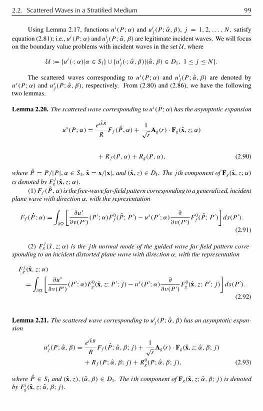
2.2. Scattered Waves in a Stratified Medium 99
Using Lemma 2.17, functions ui(P ;α) and uij (P ; α, β), j = 1, 2, . . . , N, satisfyequation (2.81); i.e., ui(P ;α) and uij (P ; α, β) are legitimate incident waves. We will focuson the boundary value problems with incident waves in the set U , where
U := ui(·;α)|α ∈ S1 ∪ uij (·; α, β)|(α, β) ∈ D1, 1 ≤ j ≤ N.
The scattered waves corresponding to ui(P ;α) and uij (P ; α, β) are denoted byus(P ;α) and usj (P ; α, β), respectively. From (2.80) and (2.86), we have the followingtwo lemmas.
Lemma 2.20. The scattered wave corresponding to ui(P ;α) has the asymptotic expansion
us(P ;α) = eikR
RFf (P , α)+ 1√
rAg(r) · Fg(x, z;α)
+ Rf (P, α)+ Rg(P, α), (2.90)
where P = P/|P |, α ∈ S1, x = x/|x|, and (x, z) ∈ D1. The j th component of Fg(x, z;α)is denoted by Fjg (x, z;α).
(1)Ff (P , α) is the free-wave far-field pattern corresponding to a generalized, incidentplane wave with direction α, with the representation
Ff (P ;α) =∫∂
[∂us
∂ν(P ′)(P ′;α)F 0
f (P ;P ′)− us(P ′;α) ∂
∂ν(P ′)F 0f (P ;P ′)
]ds(P ′).
(2.91)
(2) F jg (x, z;α) is the j th normal mode of the guided-wave far-field pattern corre-sponding to an incident distorted plane wave with direction α, with the representation
Fjg (x, z;α)=∫∂
[∂us
∂ν(P ′)(P ′;α)F 0
g (x, z;P ′; j)− us(P ′;α) ∂
∂ν(P ′)F 0g (x, z;P ′; j)
]ds(P ′).
(2.92)
Lemma 2.21. The scattered wave corresponding to uij (P ; α, β) has an asymptotic expan-sion
usj (P ; α, β) = eikR
RFf (P ; α, β; j)+ 1√
rAg(r) · Fg(x, z; α, β; j)
+ Rf (P ; α, β; j)+ R0g(P ; α, β; j), (2.93)
where P ∈ S1 and (x, z), (α, β) ∈ D1. The ith component of Fg(x, z; α, β; j) is denotedby F ig(x, z; α, β; j).
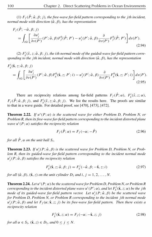
100 Chapter 2. Direct Scattering Problems in Ocean Environments
(1) Ff (P ; α, β; j), the free-wave far-field pattern corresponding to the j th incident,normal mode with direction (α, β), has the representation
Ff (P ;−α, β; j)=∫∂
[∂usj
∂ν(P ′)(P ′; α, β)F 0
f (P ;P ′)− usj (P ′; α, β) ∂
∂ν(P ′)F 0f (P ;P ′)
]ds(P ′).
(2.94)
(2) F ig(x, z; α, β; j), the ith normal mode of the guided-wave far-field pattern corre-sponding to the j th incident, normal mode with direction (α, β), has the representation
F ig(x, z; α, β; j)
=∫∂
[∂usj
∂ν(P ′)(P ′; α, β)F 0
g (x, z;P ′; i)− usj (P ′; α, β) ∂
∂ν(P ′)F 0g (x, z;P ′; i)
]ds(P ′).
(2.95)
There are reciprocity relations among far-field patterns Ff (P ;α), F ig(x, z;α),Ff (P ; α, β; j), and F ig(x, z; α, β; j). We list the results here. The proofs are similarto that in a wave guide. For detailed proof, see [470], [473], [472].
Theorem 2.22. If us(P ;α) is the scattered wave for either Problem D, Problem N, orProblem R, then its free-wave far-field pattern corresponding to the incident distorted planewave ui(P ;α) satisfies the reciprocity relation
Ff (P ;α) = Ff (−α;−P ) (2.96)
for all P , α on the unit ball S1.
Theorem 2.23. If usj (P ; α, β) is the scattered wave for Problem D, Problem N, or Prob-lem R, then its guided-wave far-field pattern corresponding to the incident normal modeuij (P ; α, β) satisfies the reciprocity relation
F ig(x, z; α, β; j) = Fjg (−α, β;−x, z; i) (2.97)
for all (α, β), (x, z) on the unit cylinder D1 and i, j = 1, 2, . . . , N .
Theorem 2.24. Let us(P ;α) be the scattered wave for Problem D, Problem N, or Problem Rcorresponding to the incident distorted plane wave ui(P ′;α), and let Fjg (x, z;α) be the j thmode of its guided-wave far-field pattern vector. Let usj (P ; α, β) be the scattered wavefor Problem D, Problem N, or Problem R corresponding to the incident j th normal modeuij (P ; α, β) and let Ff (α; x, z; j) be its free-wave far-field pattern. Then there exists areciprocity relation
Fjg (x, z;α) = Ff (−α;−x, z; j) (2.98)
for all α ∈ S1, (x, z) ∈ D1, and 0 ≤ j ≤ N .
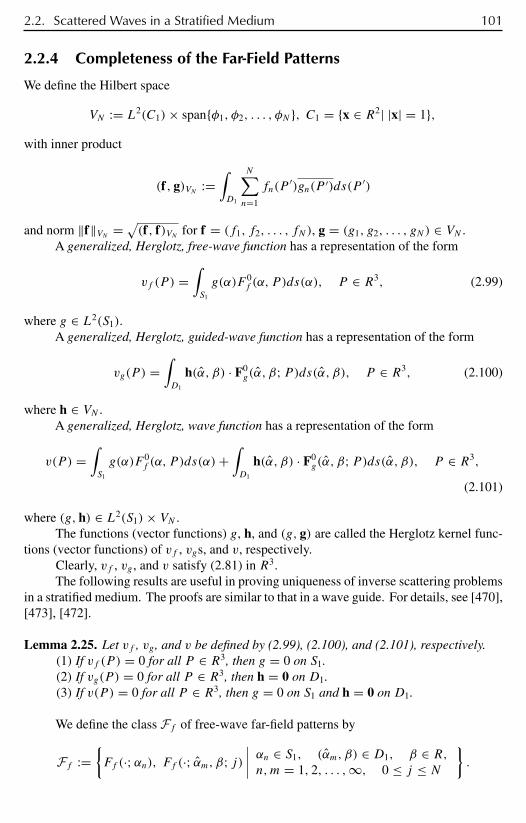
2.2. Scattered Waves in a Stratified Medium 101
2.2.4 Completeness of the Far-Field Patterns
We define the Hilbert space
VN := L2(C1)× spanφ1, φ2, . . . , φN , C1 = x ∈ R2| |x| = 1,with inner product
(f , g)VN :=∫D1
N∑n=1
fn(P′)gn(P ′)ds(P ′)
and norm ‖f‖VN = √(f , f)VN for f = (f1, f2, . . . , fN), g = (g1, g2, . . . , gN) ∈ VN .
A generalized, Herglotz, free-wave function has a representation of the form
vf (P ) =∫S1
g(α)F 0f (α, P )ds(α), P ∈ R3, (2.99)
where g ∈ L2(S1).A generalized, Herglotz, guided-wave function has a representation of the form
vg(P ) =∫D1
h(α, β) · F0g(α, β;P)ds(α, β), P ∈ R3, (2.100)
where h ∈ VN .A generalized, Herglotz, wave function has a representation of the form
v(P ) =∫S1
g(α)F 0f (α, P )ds(α)+
∫D1
h(α, β) · F0g(α, β;P)ds(α, β), P ∈ R3,
(2.101)
where (g, h) ∈ L2(S1)× VN .The functions (vector functions) g, h, and (g, g) are called the Herglotz kernel func-
tions (vector functions) of vf , vgs, and v, respectively.Clearly, vf , vg , and v satisfy (2.81) in R3.The following results are useful in proving uniqueness of inverse scattering problems
in a stratified medium. The proofs are similar to that in a wave guide. For details, see [470],[473], [472].
Lemma 2.25. Let vf , vg , and v be defined by (2.99), (2.100), and (2.101), respectively.(1) If vf (P ) = 0 for all P ∈ R3, then g = 0 on S1.(2) If vg(P ) = 0 for all P ∈ R3, then h = 0 on D1.(3) If v(P ) = 0 for all P ∈ R3, then g = 0 on S1 and h = 0 on D1.
We define the class Ff of free-wave far-field patterns by
Ff :=Ff (·;αn), Ff (·; αm, β; j)
∣∣∣∣ αn ∈ S1, (αm, β) ∈ D1, β ∈ R,n,m = 1, 2, . . . ,∞, 0 ≤ j ≤ N
.
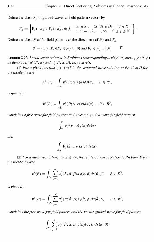
102 Chapter 2. Direct Scattering Problems in Ocean Environments
Define the class Fg of guided-wave far-field pattern vectors by
Fg :=
Fg(·;αn), Fg(·; αm, β; j)∣∣∣∣ αn ∈ S1, (α, β) ∈ D1, β ∈ R,n,m = 1, 2, . . . ,∞, 0 ≤ j ≤ N
.
Define the class F of far-field patterns as the direct sum of Ff and FgF = (Ff ,Fg)|Ff ∈ Ff ∪ 0 and Fg ∈ Fg ∪ 0.
Lemma 2.26. Let the scattered wave in Problem D corresponding toui(P ;α)anduij (P ; α, β)be denoted by us(P ;α) and usj (P ; α, β), respectively.
(1) For a given function g ∈ L2(S1), the scattered wave solution to Problem D forthe incident wave
vi(P ) =∫S1
ui(P ;α)g(α)ds(α), P ∈ R3,
is given by
vs(P ) =∫S1
us(P ;α)g(α)ds(α), P ∈ R3,
which has a free-wave far-field pattern and a vector, guided-wave far-field pattern∫S1
Ff (P , α)g(α)ds(α)
and ∫S1
Fg(x, z;α)g(α)ds(α).
(2) For a given vector function h ∈ VN , the scattered wave solution to Problem D forthe incident wave
vi(P ) =∫D1
N∑j=1
uij (P ; α, β)hj (α, β)ds(α, β), P ∈ R3,
is given by
vs(P ) =∫D1
N∑j=1
usj (P ; α, β)hj (α, β)ds(α, β), P ∈ R3,
which has the free-wave far-field pattern and the vector, guided-wave far-field pattern∫D1
N∑j=1
Ff (P ; α, β; j)hj (α, β)ds(α, β),
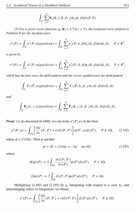
2.2. Scattered Waves in a Stratified Medium 103
∫D1
N∑j=1
Fg(x, z; α, β; j)hj (α, β)ds(α, β).
(3) For a given vector function (g, h) ∈ L2(S1)× VN the scattered wave solution toProblem D for the incident wave
vi(P ) =∫S1
ui(P ;α)g(α)ds(α)+∫D1
N∑j=1
uij (P ; α, β)hj (α, β)ds(α, β), P ∈ R3,
is given by
vs(P ) =∫S1
us(P ;α)g(α)ds(α)+∫D1
N∑j=1
usj (P ; α, β)hj (α, β)ds(α, β), P ∈ R3,
which has the free-wave far-field pattern and the vector, guided-wave far-field pattern∫S1
Ff (P , α)g(α)ds(α)+∫D1
N∑j=1
Ff (P ; α, β; j)hj (α, β)ds(α, β)
and ∫S1
Fg(x, z;α)g(α)ds(α)+∫D1
N∑j=1
Fg(x, z; α, β; j)hj (α, β)ds(α, β).
Proof. (1) As discussed in [468], we can write us(P ;α) in the form
us(P ;α) =∫∂
[∂G
∂ν(P ;P ′)+ iλG(P ;P ′)
]φ(P ′;α)ds(P ′), P /∈ ∂, (2.102)
where φ ∈ C(∂). Then φ satisfies
φ + (K + iλS)φ = −2ui on ∂, (2.103)
where
(Kφ)(P ) := 2∫∂
∂G(P ;P ′)∂ν(P ′)
φ(P ′)ds(P ′), P ∈ ∂,
(Sφ)(P ) := 2∫∂
G(P ;P ′)φ(P ′)ds(P ′), P ∈ ∂.
Multiplying (2.102) and (2.103) by g, integrating with respect to α over S1, andinterchanging orders of integration, we obtain
vs(P ) =∫∂
[∂G
∂ν(P ;P ′)+ iλG(P ;P ′)
]ψ(P ′)ds(P ′), P /∈ ∂,
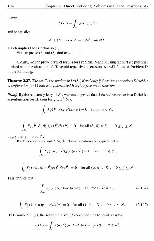
104 Chapter 2. Direct Scattering Problems in Ocean Environments
where
ψ(P ′) =∫S1
φ(P ′;α)dαand ψ satisfies
ψ + (K + iλS)ψ = −2vi on ∂,
which implies the assertion in (1).We can prove (2) and (3) similarly.
Clearly, we can prove parallel results for Problems N and R using the surface potentialmethod as in the above proof. To avoid repetitive discussion, we will focus on Problem Din the following.
Theorem 2.27. The set Ff is complete inL2(S1) if and only if there does not exist a Dirichleteigenfunction for that is a generalized Herglotz free-wave function.
Proof. By the real analyticity of Ff , we need to prove that if there does not exist a Dirichleteigenfunction for , then for g ∈ L2(S1),∫
S1
Ff (P ;α)g(P )ds(P ) = 0 for all α ∈ S1,
∫S1
Ff (P ; α, β; j)g(P )ds(P ) = 0 for all (α, β) ∈ D1, 0 ≤ j ≤ N,
imply that g = 0 on S1.By Theorems 2.22 and 2.24, the above equations are equivalent to∫
S1
Ff (−α;−P )g(P )ds(P ) = 0 for all α ∈ S1,
∫S1
F jg (−α, β;−P )g(P )ds(P ) = 0 for all (α, β) ∈ D1, 0 ≤ j ≤ N.
This implies that ∫S1
Ff (P ;α)g(−α)ds(α) = 0 for all P ∈ S1, (2.104)
∫S1
F jg (x, z;α)g(−α)ds(α) = 0 for all (x, z) ∈ D1, 0 ≤ j ≤ N. (2.105)
By Lemma 2.26 (1), the scattered wave us corresponding to incident wave
vi(P ) =∫S1
g(α)F 0f (α;P)ds(α) = vf (P ), P ∈ R3,

2.2. Scattered Waves in a Stratified Medium 105
has vanishing far-field patterns given by (2.100) and (2.105), whence us is identical to zeroin R3 \. By the Dirichlet boundary condition vf ≡ vi = −us = 0 on ∂. Hence vf = 0in R3, for there does not exist any Dirichlet eigenfunction for . From Lemma 2.25 (1) itfollows that g = 0 on S1.
Theorem 2.28. The set Fg is complete in VN if and only if there does not exist a Dirichleteigenfunction for that is a generalized Herglotz guided-wave function.
Proof. We want to prove that if there does not exist a Dirichlet eigenfunction for , thenfor h ∈ VN , we may conclude that h = 0 from
N∑j=1
∫D1
F jg (x, z;α)hj (x, z)ds(x, z) = 0 for all α ∈ S1, (2.106)
N∑j=1
∫D1
F jg (x, z; α, β; i)hj (P )ds(P ) = 0, i = 1, 2, . . . , N, for all (x, z) ∈ D1.
(2.107)
By Theorem 2.23, equations (2.106) and (2.107) are equivalent to
N∑j=1
∫D1
Ff (P ; α, β; j)hj (−α, β)ds(α, β) = 0 for all P ∈ S1,
N∑j=1
∫D1
F ig(x, z; α, β; j)hj (α, β)ds(α, β) = 0, i = 1, 2, . . . , N, for all (x, z) ∈ D1.
By Lemma 2.26 (2), the scattered wave corresponding to incident wave
vi(P ) =N∑j=1
∫D1
Fg
0 (α, β;P ; j)hj (α, β)ds(α, β) = vg(P ), P ∈ R3,
has vanished far-field patterns. Using the same argument as in the proof of Theorem 2.27,we know that vg ≡ 0 in R3, hence h = 0 on D1 by Lemma 2.25 (2).
Using similar proofs as in Theorems 2.27 and 2.28, we can show the following.
Theorem 2.29. The set F is complete in L2(S1)× VN if and only if there does not exist aDirichlet eigenfunction for that is a generalized Herglotz function.
Since the free-wave and guided-wave solutions are linearly independent, we have thefollowing corollary.
Corollary 2.30. If k is a simple Dirichlet eigenvalue in , then either Ff is complete inL2(S1) or Fg is complete in VN .


Chapter 3
Inverse Scattering Problemsin Ocean Environments
3.1 Inverse Scattering Problems in Homogeneous OceansThe inverse scattering problem for acoustic waves consists of recovering the shape of a scat-terer from the scattered field. Inverse problems have inspired a wide variety of techniquesin the engineering sciences, such as remote sensing, nondestructive testing, and imagingetc., and for this reason have been the object of study by scientists in a number of diversedisciplines. Rapid progress in this field has been made since the early 1970s, and a surveyof these results can be found in [126], [121], and the references cited there. However, mostof the activity in this field has been directed to the cases of R2 and R3. It has been noticedthat in some situations, for example, in a wave guide, remote sensing and imaging lead tomore complicated problems. In a homogeneous, finite-depth ocean, Gilbert and Xu [211],[210] showed6 that the “propagating’’ far-field pattern can carry only the information fromtheN+1 propagating modes, whereN is the largest integer less than (2kh−π)/2π and h isthe depth of the ocean. This loss of information makes this problem different from inverseproblems in Rn since the far-field pattern operator is no longer injective. A particular ex-ample of this occurs for 0 < k < π/2h; thenN = −1 and the far-field pattern is identicallyzero for any incoming waves. Even in the case of sufficiently large k, the vanished far-fieldpattern only implies that the N + 1 propagating modes are identically zero. Therefore, thefar-field pattern operator F is not an injection on the Hilbert space L2(∂).
In Chapter 2, section 2.1.11 we established theoretical results for constructing aninjective far-field operator. These results are essential for finding a generalized inverse forF. In section 3.1 we consider the following problem: Given the far-field pattern f (x, z, k)for one or several incoming (entire) waves ui , find the shape of the scattering object .Other inverse problems are considered in the following sections.
6See also Chapter 2 of the present work.
107
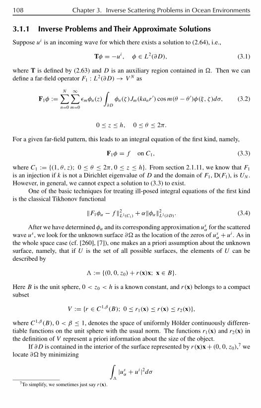
108 Chapter 3. Inverse Scattering Problems in Ocean Environments
3.1.1 Inverse Problems and Their Approximate Solutions
Suppose ui is an incoming wave for which there exists a solution to (2.64), i.e.,
Tφ = −ui, φ ∈ L2(∂D), (3.1)
where T is defined by (2.63) and D is an auxiliary region contained in . Then we candefine a far-field operator F1 : L2(∂D)→ V N as
F1φ :=N∑n=0
∞∑m=0
εmφn(z)
∫∂D
φn(ζ )Jm(kanr′) cosm(θ − θ ′)φ(ξ, ζ )dσ, (3.2)
0 ≤ z ≤ h, 0 ≤ θ ≤ 2π.
For a given far-field pattern, this leads to an integral equation of the first kind, namely,
F1φ = f on C1, (3.3)
where C1 := (1, θ, z); 0 ≤ θ ≤ 2π, 0 ≤ z ≤ h. From section 2.1.11, we know that F1
is an injection if k is not a Dirichlet eigenvalue of D and the domain of F1, D(F1), is UN .However, in general, we cannot expect a solution to (3.3) to exist.
One of the basic techniques for treating ill-posed integral equations of the first kindis the classical Tikhonov functional
‖F1φα − f ‖2L2(C1)
+ α‖φα‖2L2(∂D). (3.4)
After we have determined φα and its corresponding approximation usα for the scatteredwave us , we look for the unknown surface ∂ as the location of the zeros of usα + ui . As inthe whole space case (cf. [260], [7]), one makes an a priori assumption about the unknownsurface, namely, that if U is the set of all possible surfaces, the elements of U can bedescribed by
:= (0, 0, z0)+ r(x)x; x ∈ B.Here B is the unit sphere, 0 < z0 < h is a known constant, and r(x) belongs to a compactsubset
V := r ∈ C1,β(B); 0 ≤ r1(x) ≤ r(x) ≤ r2(x),where C1,β(B), 0 < β ≤ 1, denotes the space of uniformly Hölder continuously differen-tiable functions on the unit sphere with the usual norm. The functions r1(x) and r2(x) inthe definition of V represent a priori information about the size of the object.
If ∂D is contained in the interior of the surface represented by r(x)x + (0, 0, z0),7 welocate ∂ by minimizing ∫
|usα + ui |2dσ7To simplify, we sometimes just say r(x).
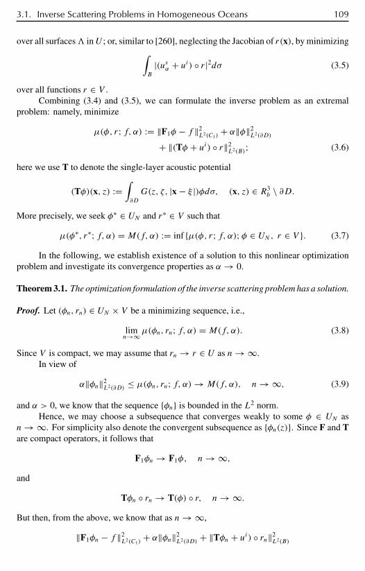
3.1. Inverse Scattering Problems in Homogeneous Oceans 109
over all surfaces inU ; or, similar to [260], neglecting the Jacobian of r(x), by minimizing∫B
|(usα + ui) r|2dσ (3.5)
over all functions r ∈ V .Combining (3.4) and (3.5), we can formulate the inverse problem as an extremal
problem: namely, minimize
µ(φ, r; f, α) := ‖F1φ − f ‖2L2(C1)
+ α‖φ‖2L2(∂D)
+ ‖(Tφ + ui) r‖2L2(B); (3.6)
here we use T to denote the single-layer acoustic potential
(Tφ)(x, z) :=∫∂D
G(z, ζ, |x − ξ |)φdσ, (x, z) ∈ R3b \ ∂D.
More precisely, we seek φ∗ ∈ UN and r∗ ∈ V such that
µ(φ∗, r∗; f, α) = M(f, α) := inf µ(φ, r; f, α);φ ∈ UN, r ∈ V . (3.7)
In the following, we establish existence of a solution to this nonlinear optimizationproblem and investigate its convergence properties as α → 0.
Theorem 3.1. The optimization formulation of the inverse scattering problem has a solution.
Proof. Let (φn, rn) ∈ UN × V be a minimizing sequence, i.e.,
limn→∞µ(φn, rn; f, α) = M(f, α). (3.8)
Since V is compact, we may assume that rn → r ∈ U as n→ ∞.In view of
α‖φn‖2L2(∂D) ≤ µ(φn, rn; f, α)→ M(f, α), n→ ∞, (3.9)
and α > 0, we know that the sequence φn is bounded in the L2 norm.Hence, we may choose a subsequence that converges weakly to some φ ∈ UN as
n→ ∞. For simplicity also denote the convergent subsequence as φn(z). Since F and Tare compact operators, it follows that
F1φn → F1φ, n→ ∞,and
Tφn rn → T(φ) r, n→ ∞.But then, from the above, we know that as n→ ∞,
‖F1φn − f ‖2L2(C1)
+ α‖φn‖2L2(∂D) + ‖Tφn + ui) rn‖2
L2(B)

110 Chapter 3. Inverse Scattering Problems in Ocean Environments
→ ‖F1φ − f ‖2L2(C1)
+ α‖φ‖2L2(∂D) + ‖Tφ + ui) r‖2
L2(B);hence,
‖φn‖2L2(∂D) → ‖φ‖2
L2(∂D), n→ ∞.This, together with the weak convergence, implies that
‖φn − φ‖2L2(∂D) =
∫∂D
|φn(ξ, ζ )− φ(ξ, ζ )|2dσ
=∫∂D
|φn(ξ, ζ )|2dσ +∫∂D
|φ(ξ, ζ )|2dσ − 2Re∫∂D
φn(ξ, ζ )φ(ξ, ζ )dσ
→ 2∫∂D
|φ(ξ, ζ )|2dσ − 2Re∫∂D
φ(ξ, ζ )φ(ξ, ζ )dσ = 0 as n→ ∞, (3.10)
and φ ∈ UN since UN is a closed set. Hence,
µ(φ, r; f, α) = limn→∞µ(φn, rn; f, α) = M(f, α). (3.11)
This completes the proof.
Theorem 3.2. Let ui ∈ B(N, ∂) and f0 be the corresponding far-field pattern of a domain∂ that described by some r ∈ V . Then
limα→0
M(f0, α) = 0.
Proof. Let ε > 0 be arbitrary. Then there exists φ ∈ UN such that
‖Tφ + ui) r‖L2(B) < ε,
due toui ∈ B(N, ∂). Since the far-field pattern of the scattered wave depends continuouslyon the boundary data us , we can find a constant depending on ∂, C = C(∂), such that
‖F1φ − f0‖L2() ≤ C‖Tφ − us) r‖L2(B). (3.12)
Since ui + us = 0 on ∂, we have
µ(φ, r; f0, α) ≤ (1 + C)‖(Tφ + ui) r‖L2(B) + α‖φ‖L2(∂D)
≤ (1 + C)ε + α‖φ‖ → (1 + C)ε as α → 0.
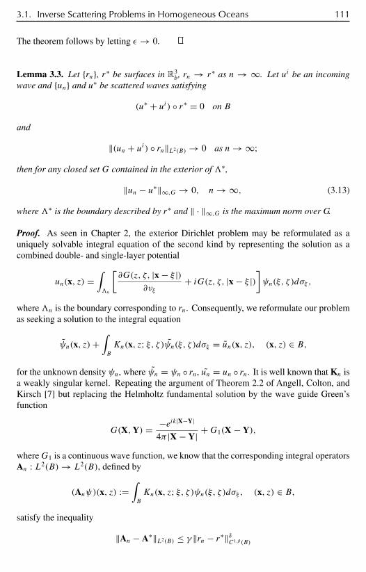
3.1. Inverse Scattering Problems in Homogeneous Oceans 111
The theorem follows by letting ε → 0.
Lemma 3.3. Let rn, r∗ be surfaces in R3b, rn → r∗ as n → ∞. Let ui be an incoming
wave and un and u∗ be scattered waves satisfying
(u∗ + ui) r∗ = 0 on B
and
‖(un + ui) rn‖L2(B) → 0 as n→ ∞;then for any closed set G contained in the exterior of ∗,
‖un − u∗‖∞,G → 0, n→ ∞, (3.13)
where ∗ is the boundary described by r∗ and ‖ · ‖∞,G is the maximum norm over G.
Proof. As seen in Chapter 2, the exterior Dirichlet problem may be reformulated as auniquely solvable integral equation of the second kind by representing the solution as acombined double- and single-layer potential
un(x, z) =∫n
[∂G(z, ζ, |x − ξ |)
∂νξ+ iG(z, ζ, |x − ξ |)
]ψn(ξ, ζ )dσξ ,
where n is the boundary corresponding to rn. Consequently, we reformulate our problemas seeking a solution to the integral equation
ψn(x, z)+∫B
Kn(x, z; ξ, ζ )ψn(ξ, ζ )dσξ = un(x, z), (x, z) ∈ B,
for the unknown density ψn, where ψn = ψn rn, un = un rn. It is well known that Kn isa weakly singular kernel. Repeating the argument of Theorem 2.2 of Angell, Colton, andKirsch [7] but replacing the Helmholtz fundamental solution by the wave guide Green’sfunction
G(X,Y) = −eik|X−Y|
4π |X − Y| +G1(X − Y),
whereG1 is a continuous wave function, we know that the corresponding integral operatorsAn : L2(B)→ L2(B), defined by
(Anψ)(x, z) :=∫B
Kn(x, z; ξ, ζ )ψn(ξ, ζ )dσξ , (x, z) ∈ B,
satisfy the inequality
‖An − A∗‖L2(B) ≤ γ ‖rn − r∗‖δC1,β (B)

112 Chapter 3. Inverse Scattering Problems in Ocean Environments
for 0 < δ < β(β + 1) with some constant γ .Consequently, we obtain the following error estimate:
‖ψn − ψ∗‖L2(B) = ‖(I + An)−1un rn − (I + A∗)−1ui r∗‖L2(B)
≤ ‖(I + An)−1(un − ui) rn‖L2(B) + ‖(I + A∗)−1ui (rn − r∗)‖L2(B)
+ ‖[(I + An)−1 − (I + A∗)−1]ui rn‖L2(B)
≤ ‖(I + An)−1(un − ui) rn‖L2(B) + ‖(I + A∗)−1ui (rn − r∗)‖L2(B)
+ ‖(I + An)−1‖ ‖A∗ − An‖ ‖(I + A∗)−1‖ ‖ui rn‖L2(B)
→ 0 as n→ ∞,
where we have used the fact that (I + An)−1 is uniformly bounded for n (see the proof ofTheorem 2.2 in [7]). Substituting this into the combined double- and single-layer potential,it follows that for each closed set G contained in the exterior of ∗,
‖un − u∗‖∞,G → 0 as n→ ∞.
This may be summarized as follows.
Theorem 3.4. Let ui ∈ B(N, ∂) be an incoming wave such that ui |∂ ∈ T UN and fbe the corresponding far-field pattern of a domain , and let (φn, rn) be a solution to theminimization problem with regularization parameter αn. Then there exists a convergentsubsequence of the sequence rn. There is only a finite number of limit points, and everylimit point represents a surface on which the total field us + ui vanishes.
Proof. From the compactness of V, there exists a convergent subsequence of rn whichconverges to, say, r∗. For simplicity we also denote this subsequence as rn so that rn → r∗as n→ ∞. Let u∗ denote the unique solution to the direct scattering problem for the objectwith boundary ∗ parameterized by r∗. Then
(u∗ + ui) r∗ = 0 on B. (3.14)
The function un corresponds to the solution of an exterior Dirichlet problem with boundaryvalues Tφn|n on a boundary n described by rn.
From Lemma 3.3, we know the far-field patterns F1φn of un converge uniformly tothe far-field pattern f ∗ of u∗, since
‖F1φn − f ∗‖L2(C1) ≤ C‖Tφn − u∗‖L2(∂)

3.1. Inverse Scattering Problems in Homogeneous Oceans 113
≤ C‖un − u∗‖∞,∂ → 0 as n→ ∞.Moreover, by Theorem 3.1,
‖F1φn − f ‖L2(C1) → 0 as n→ ∞.Therefore, we conclude that the far-field patterns coincide:
f = f ∗.
Recall that f is the far-field pattern with respect to an incoming wave ui ∈ B(N, ∂)such that Tφ = −ui admits a solution φ0 ∈ UN ; therefore, we can represent the scatteredwave as
us(x, z) = (Tφ0)(x, z), (x, z) ∈ R3b \.
Since f = F1φ0,
‖F1(φn − φ0)‖L2(C1) = ‖F1φn − f ‖L2(C1) → 0 as n→ ∞; (3.15)
it is implied from (3.15) that∫∂D
[φn − φ0][φn(ζ )Jm(kanr ′) cos(mθ ′)]dσ → 0,
∫∂D
[φn − φ0][φn(ζ )Jm(kanr ′) sin(mθ ′)]dσ → 0
as n→ ∞.It follows immediately that for any closed set G ⊂ R3
b \D,
‖Tφn − us‖∞,G = ‖T(φn − φ0)‖∞,G → 0 as n→ ∞. (3.16)
Consequently,
‖us − u∗‖∞,G ≤ ‖us − Tφn‖∞,G + ‖Tφn − u∗‖∞,G
= ‖T(φn − φ0)‖∞,G + ‖un − u∗‖∞,G → 0, n→ ∞, (3.17)
due to (3.15) and (3.17), where G is any closed set in R3b \ D. In view of (3.17) and
u∗ + ui = 0 on ∗ with ∗ ⊂ R3b \D, we can conclude that
us + ui = 0 on ∗. (3.18)
If there existed an infinite number of different limit points, then by the compactnessof V we could find a cluster point of these limit points. Thus, it would follow that there was
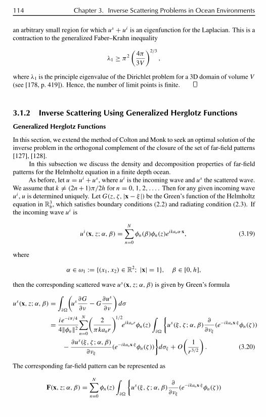
114 Chapter 3. Inverse Scattering Problems in Ocean Environments
an arbitrary small region for which us + ui is an eigenfunction for the Laplacian. This is acontraction to the generalized Faber–Krahn inequality
λ1 ≥ π2
(4π
3V
)2/3
,
where λ1 is the principle eigenvalue of the Dirichlet problem for a 3D domain of volume V(see [178, p. 419]). Hence, the number of limit points is finite.
3.1.2 Inverse Scattering Using Generalized Herglotz Functions
Generalized Herglotz Functions
In this section, we extend the method of Colton and Monk to seek an optimal solution of theinverse problem in the orthogonal complement of the closure of the set of far-field patterns[127], [128].
In this subsection we discuss the density and decomposition properties of far-fieldpatterns for the Helmholtz equation in a finite depth ocean.
As before, let u = ui + us , where ui is the incoming wave and us the scattered wave.We assume that k = (2n+ 1)π/2h for n = 0, 1, 2, . . . . Then for any given incoming waveui , u is determined uniquely. LetG(z, ζ, |x − ξ |) be the Green’s function of the Helmholtzequation in R3
b, which satisfies boundary conditions (2.2) and radiating condition (2.3). Ifthe incoming wave ui is
ui(x, z;α, β) =N∑n=0
φn(β)φn(z)eikanα·x, (3.19)
where
α ∈ ω1 := (x1, x2) ∈ R2; |x| = 1, β ∈ [0, h],then the corresponding scattered wave us(x, z;α, β) is given by Green’s formula
us(x, z;α, β) =∫∂
(us∂G
∂ν−G∂u
s
∂ν
)dσ
= ie−iπ/4
4‖φn‖2
N∑n=0
(2
πkanr
)1/2
eikanrφn(z)
∫∂
us(ξ, ζ ;α, β) ∂
∂νξ(e−ikanx·ξφn(ζ ))
− ∂us(ξ, ζ ;α, β)∂νξ
(e−ikanx·ξφn(ζ ))dσξ +O
(1
r3/2
). (3.20)
The corresponding far-field pattern can be represented as
F(x, z;α, β) =N∑n=0
φn(z)
∫∂
us(ξ, ζ ;α, β) ∂
∂νξ(e−ikanx·ξφn(ζ ))
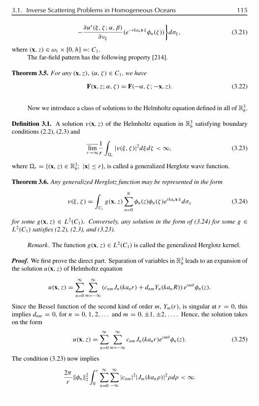
3.1. Inverse Scattering Problems in Homogeneous Oceans 115
−∂us(ξ, ζ ;α, β)∂νξ
(e−ikanx·ξφn(ζ ))dσξ , (3.21)
where (x, z) ∈ ω1 × [0, h] =: C1.
The far-field pattern has the following property [214].
Theorem 3.5. For any (x, z), (α, ζ ) ∈ C1, we have
F(x, z;α, ζ ) = F(−α, ζ ;−x, z). (3.22)
Now we introduce a class of solutions to the Helmholtz equation defined in all of R3b.
Definition 3.1. A solution v(x, z) of the Helmholtz equation in R3b satisfying boundary
conditions (2.2), (2.3) and
limr→∞
1
r
∫r
|v(ξ, ζ )|2dξdζ <∞, (3.23)
where r = (x, z) ∈ R3b; |x| ≤ r, is called a generalized Herglotz wave function.
Theorem 3.6. Any generalized Herglotz function may be represented in the form
v(ξ, ζ ) =∫C1
g(x, z)N∑n=0
φn(z)φn(ζ )eikanx·ξ dσx (3.24)
for some g(x, z) ∈ L2(C1). Conversely, any solution in the form of (3.24) for some g ∈L2(C1) satisfies (2.2), (2.3), and (3.23).
Remark. The function g(x, z) ∈ L2(C1) is called the generalized Herglotz kernel.
Proof. We first prove the direct part. Separation of variables in R3b leads to an expansion of
the solution u(x, z) of Helmholtz equation
u(x, z) =∞∑n=0
∞∑m=−∞
(cnmJn(kanr)+ dnmYn(kanR)) eimθφn(z).
Since the Bessel function of the second kind of order m, Ym(r), is singular at r = 0, thisimplies dnm = 0, for n = 0, 1, 2, . . . and m = 0,±1,±2, . . . . Hence, the solution takeson the form
u(x, z) =∞∑n=0
∞∑m=−∞
cnmJn(kanr)eimθφn(z). (3.25)
The condition (3.23) now implies
2π
r‖φn‖2
2
∫ r
0
∞∑n=0
∞∑−∞
|cnm|2|Jm(kanρ)|2ρdρ <∞.

116 Chapter 3. Inverse Scattering Problems in Ocean Environments
Note that for any integer n > N , where N = [(2kh − π)/2π ], an defined by (2.6) is animaginary number. Using the asymptotic expansion
Jm(kanr) ≈√
1
2πkanr
(e−ikanr+i(m+1/2)π/2 + eikanr−i(m+1/2)π/2
),
we realize that since Jm(kanr)/√r → ∞ as r → ∞, then cnm = 0 for any n > N and
m = 0,±1,±2, . . . . From this, (3.25) reduces to a propagating wave of the form
u(x, z) =N∑n=0
∞∑m=−∞
cnmJn(kanr)eimθφn(z). (3.26)
To show that v(x, z) may be written in the form (3.24), we rewrite (3.24) as
v(x, z) =N∑n=0
∫ h
0
∫ 2π
0g(φ, ζ )φn(z)φn(ζ )e
−ikanr cos(θ−φ)dφdζ,
where r = |x| and (r, θ, z) are the cylindrical coordinates of (x, z). Using the Jacobi–Angerexpansion
e−kanrcos(θ−φ) =∞∑
m=−∞(−i)mJm(kanr)eim(θ−φ),
we rewrite v(x, z) as
v(x, z) =N∑n=0
∞∑m=−∞
φn(z)eimθJm(kanr)
[∫ h
0
∫ 2π
0(−i)me−imφφn(ζ )g(φ, ζ )dφdζ
].
(3.27)
Now if g(φ, ζ ) is defined to be the function given by the series
g(φ, ζ ) =N∑n=0
∞∑m=−∞
imcnm
2πφn(ζ )e
imφ,
then u(x, z) ≡ v(x, z). Moreover, since∫ h
0
∫ 2π
0|g(φ, ζ )|2dφdζ = 1
2π
N∑n=0
∞∑m=−∞
|cnm|2 · ‖φn‖2
= h
4π
N∑n=0
∞∑m=−∞
|cnm|2, (3.28)
we may show that g(φ, ζ ) ∈ L2(C1) if (3.28) is bounded. From (3.23) we have
N∑n=0
∞∑m=−∞
|cnm|2(
1
r
∫ r
0|Jm(kanρ)|2ρdρ
)<∞.
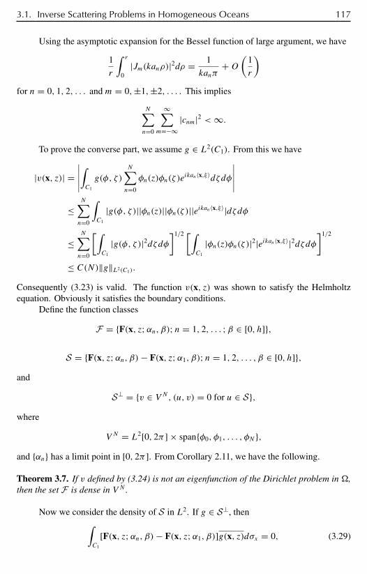
3.1. Inverse Scattering Problems in Homogeneous Oceans 117
Using the asymptotic expansion for the Bessel function of large argument, we have
1
r
∫ r
0|Jm(kanρ)|2dρ = 1
kanπ+O
(1
r
)for n = 0, 1, 2, . . . and m = 0,±1,±2, . . . . This implies
N∑n=0
∞∑m=−∞
|cnm|2 <∞.
To prove the converse part, we assume g ∈ L2(C1). From this we have
|v(x, z)| =∣∣∣∣∣∫C1
g(φ, ζ )
N∑n=0
φn(z)φn(ζ )eikan〈x,ξ〉dζdφ
∣∣∣∣∣≤
N∑n=0
∫C1
|g(φ, ζ )||φn(z)||φn(ζ )||eikan〈x,ξ〉|dζdφ
≤N∑n=0
[∫C1
|g(φ, ζ )|2dζdφ]1/2 [∫
C1
|φn(z)φn(ζ )|2|eikan〈x,ξ〉|2dζdφ]1/2
≤ C(N)‖g‖L2(C1).
Consequently (3.23) is valid. The function v(x, z) was shown to satisfy the Helmholtzequation. Obviously it satisfies the boundary conditions.
Define the function classes
F = F(x, z;αn, β); n = 1, 2, . . . ;β ∈ [0, h],
S = F(x, z;αn, β)− F(x, z;α1, β); n = 1, 2, . . . , β ∈ [0, h],and
S⊥ = v ∈ V N, (u, v) = 0 for u ∈ S,where
V N = L2[0, 2π ] × spanφ0, φ1, . . . , φN ,and αn has a limit point in [0, 2π ]. From Corollary 2.11, we have the following.
Theorem 3.7. If v defined by (3.24) is not an eigenfunction of the Dirichlet problem in ,then the set F is dense in V N .
Now we consider the density of S in L2. If g ∈ S⊥, then∫C1
[F(x, z;αn, β)− F(x, z;α1, β)]g(x, z)dσx = 0, (3.29)

118 Chapter 3. Inverse Scattering Problems in Ocean Environments
n = 1, 2, . . . , β ∈ [0, h].By analytic continuation of F(x, z;α, β) with respect to (α, β), it follows that for everyα ∈ ω1 ∫
C1
[F(x, z;α, β)]g(x, z)dσx =N∑n=0
cnφn(β), β ∈ [0, h], (3.30)
where the cn are constants.Suppose now that not all the cn are equal to zero, and define
Us(x, z) =∫C1
us(x, z;α, β)g(−α, β)dσα. (3.31)
Then the far-field pattern of Us(x, z) is given by∫C1
F(x, z;α, β)g(−α, β)dσα
=∫C1
F(−α, β;−x, z)g(−α, β)dσα
=N∑n=0
cnφn(z). (3.32)
Without loss of generality, we assume that cn = φn(z0), where (0, z0) is in the interior of. It follows that for |x| ≥ R, where R is a constant such that DR ⊃ ,
Us(x, z) = 2
h
N∑n=0
φn(z)φn(z0)H(1)0 (kanr)+ σN, (3.33)
where σN contains no propagating modes. However, since g ∈ S⊥ ⊂ V N , for |x| ≥ R,Us(x, z) can be expressed as
Us(x, z) =∫C1
us(x, z;α, β)g(−α, β)dσα
=N∑n=0
φn(z)Usn(x). (3.34)
Hence, we must have
Us(x, z) = 2
h
N∑n=0
φn(z)φn(z0)H(1)0 (kanr), r ≥ R. (3.35)
The importance of the above result is that even though for a given far-field pattern weusually cannot determine a unique near field, we can find a function such as Us(x, z) thatis uniquely determined by the far-field pattern∫
C1
F(x, z;α, β)g(−α, β)dσα.
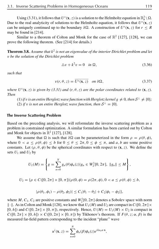
3.1. Inverse Scattering Problems in Homogeneous Oceans 119
Using (3.31), it follows thatUs(x, z) is a solution to the Helmholtz equation in R3b \.
Due to the real analyticity of solutions to the Helmholtz equation, it follows that Us(x, z)can be uniquely continued up to the boundary ∂. A construction of Us(x, z) for r ≤ R
may be found in [214].Similar to a theorem of Colton and Monk for the case of R2 [127], [128], we can
prove the following theorem. (See [214] for details.)
Theorem 3.8. Assume that k2 is not an eigenvalue of the interior Dirichlet problem and letv be the solution of the Dirichlet problem
v + k2v = 0 in , (3.36)
such that
v(r, θ, z) = Us(x, z) on ∂, (3.37)
where Us(x, z) is given by (3.31) and (r, θ, z) are the polar coordinates related to (x, z).Then
(1) if v is an entire Herglotz wave function with Herglotz kernel g = 0, then S⊥ = 0;(2) if v is not an entire Herglotz wave function, then S⊥ = 0.
The Inverse Scattering Problem
Based on the preceding analysis, we will reformulate the inverse scattering problem as aproblem in constrained optimization. A similar formulation has been carried out by Coltonand Monk for objects in R2 [127], [128].
We assume that is such that ∂ can be parameterized in the form ρ = ρ(θ, φ),where 0 < a ≤ ρ(θ, φ) ≤ b for 0 ≤ θ ≤ 2π, 0 ≤ φ ≤ π, and a, b are some positiveconstants. Let (ρ, θ, φ) be the spherical coordinates with respect to (x, z). We define thesets U1 and U2 by
U1(M) =g =
N∑n=0
gn(θ)φn(z)|gn ∈ W 12 [0, 2π ], ‖gn‖ ≤ M
,
U2 = ρ ∈ C([0, 2π ] × [0, π ])|ρ(0, φ) = ρ(2π, φ), 0 < a ≤ ρ(θ, φ) ≤ b,
|ρ(θ1, φ1)− ρ(θ2, φ2)| ≤ C1|θ1 − θ2| + C2|φ1 − φ2|,whereM,C1, C2 are positive constants andW 1
2 [0, 2π ] denotes a Sobolev space with norm‖·‖. As in Colton and Monk [128], we know thatU1(M) andU2 are compact inC([0, 2π ]×[0, h]) and C([0, 2π ] × [0, π ]), respectively. Hence, U(M) = U1(M)× U2 is compact inC([0, 2π ] × [0, h]) × C([0, 2π ] × [0, π ]) by Tikhonov’s theorem. If F(θ, z;α, β) is themeasured far-field pattern corresponding to the incident “plane’’ wave
ui(x, z) =N∑n=0
φn(β)φn(z)eikanα·x,

120 Chapter 3. Inverse Scattering Problems in Ocean Environments
then we define the optimization problem as
J (F,M, J, L) = min(g,ρ)∈U(M)
J∑j=1
L∑l=1
∣∣∣∣∣∫C1
F(x, z;αl, βj )g(x, z)dσx −N∑n=0
φn(z0)φn(βj )
∣∣∣∣∣2
+∫ π
0
∫ 2π
0|v(r(θ, φ), θ, z(θ, φ))− Us(r(θ, φ), θ, z(θ, φ))|2dθdφ
, (3.38)
where
r(θ, φ) = ρ(θ, φ) sin φ, z(θ, φ) = ρ(θ, φ) cosφ + z0.
v is defined by (3.24).
Definition 3.2. A function ρ ∈ C([0, 2π ] × [0, π ]) is said to be admissible if and only ifthe pair (g, ρ) ∈ U(M) minimizes (3.38) over U(M).
It is clear that, from the compactness of U(M) and continuity of the integral in (3.38)with respect to ρ and g, there exists at least one admissible solution.
In examining the relationship between admissible solutions and actual solutions ofthe inverse scattering problem, we can prove the following theorems in a similar way as thecorresponding theorem in [127], [128].
Theorem 3.9. Let (F) be the set of admissible solutions corresponding to the far-fieldpattern F . If Fj → F in V N , ρj ∈ (Fj ), then there exists a convergent subsequence ofρj whose every limit point lies in (F).
Proof. Since U2 is compact, without loss of generality we can assume that ρj convergesto ρ∗ ∈ U2. Let (gj , ρj ) be the corresponding pair such that the sequence (gj , ρj ) →(g∗, ρ∗) ∈ U(M). We need to show that
J (F,M, J, L) =J∑j=1
L∑l=1
∣∣∣∣∣∫C1
F(x, z;αl, βj )g∗(x, z)dσx −N∑n=0
φn(z0)φn(βj )
∣∣∣∣∣2
+∫ π
0
∫ 2π
0|v∗(r∗(θ, φ), θ, z∗(θ, φ))− Us(r∗(θ, φ), θ, z∗(θ, φ))|2dθdφ, (3.39)
where v∗ is the generalized Herglotz wave function associated with g∗, r∗ = ρ∗ sin φ andz∗ = ρ∗ cosφ. Now if ρ ∈ (F) has the corresponding pair (g, ρ), then
J (F,M, J, L) ≤J∑j=1
L∑l=1
∣∣∣∣∣∫C1
F(x, z;αl, βj )g∗(x, z)dσx −N∑n=0
φn(z0)φn(βj )
∣∣∣∣∣2
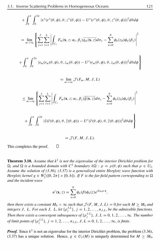
3.1. Inverse Scattering Problems in Homogeneous Oceans 121
+∫ π
0
∫ 2π
0|v∗(r∗(θ, φ), θ, z∗(θ, φ))− Us(r∗(θ, φ), θ, z∗(θ, φ))|2dθdφ
= limm→∞
J∑j=1
L∑l=1
∣∣∣∣∣∫C1
Fm(x, z;αl, βj )gm(x, z)dσx −N∑n=0
φn(z0)φn(βj )
∣∣∣∣∣2
+∫ π
0
∫ 2π
0|vm(rm(θ, φ), θ, zm(θ, φ))− Us(rm(θ, φ), θ, zm(θ, φ))|2dθdφ
= limm→∞ J (Fm,M, J, L)
≤ limm→∞
J∑j=1
L∑l=1
∣∣∣∣∣∫C1
Fm(x, z;αl, βj )g(x, z)dσx −N∑n=0
φn(z0)φn(βj )
∣∣∣∣∣2
+∫ π
0
∫ 2π
0|v(r(θ, φ), θ, z(θ, φ))− Us(r(θ, φ), θ, z(θ, φ))|2dθdφ
= J (F,M, J, L).
This completes the proof.
Theorem 3.10. Assume that k2 is not the eigenvalue of the interior Dirichlet problem for, and is a bounded domain with C2 boundary ∂ : ρ = ρ(θ, φ) such that ρ ∈ U2.Assume the solution of (3.36), (3.37) is a generalized entire Herglotz wave function withHerglotz kernel g ∈ W 1
2 ([0, 2π ] × [0, h]). If F is the far-field pattern corresponding to and the incident wave
ui(x, z) =N∑n=0
φn(β)φn(z)eikanα·x,
then there exists a constant M0 < ∞ such that J (F,M, J, L) = 0 for each M ≥ M0 andintegers J, L. For each J, L, let ρJ,Lj , j = 1, 2, . . . , nJ,L, be the admissible functions.
Then there exists a convergent subsequence of ρJ,Lj , J, L = 0, 1, 2, . . . ,∞. The number
of limit points of ρJ,Lj , j = 1, 2, . . . , nJ,L, J, L = 0, 1, 2, . . . ,∞, is finite.
Proof. Since k2 is not an eigenvalue for the interior Dirichlet problem, the problem (3.36),(3.37) has a unique solution. Hence, g ∈ U1(M) is uniquely determined for M ≥ M0,
122 Chapter 3. Inverse Scattering Problems in Ocean Environments
where M0 is a positive constant. From (3.30) and (3.37) we see that J (F,M, J, L) = 0for eachM ≥ M0 and every integer J and L.
Now let ρJ,Lj be as defined in the statement of the theorem. Then sinceU2 is compact,
the sequence ρJ,Lj has a subsequence converging to ρ∗ ∈ U2. Let gJ,Lj ∈ U1(M) be a
function associated with ρJ,Lj . Then gJ,Lj has a subsequence converging to a limit pointg∗ ∈ U1(M). But it follows from the fact that J (F,M, J, L) = 0 for M ≥ M0 and foreach J, L,
∫C1
[F(x, z;αi, βl)]gJ,Lj (x, z)dσx =N∑n=0
φn(z0)φn(βl) (3.40)
for i = 1, 2, . . . , J , l = 1, 2, . . . , L. Hence,
∫C1
[F(x, z;αi, βl)]g∗(x, z)dσx =N∑n=0
φn(z0)φn(βl) (3.41)
for i = 1, 2, . . . , l = 1, 2, . . . . In view of Theorem 3.7, F is dense in V N . Therefore, wenow can conclude that g∗ = g.
Now we prove that there is only a finite number of limit points ρ∗ lying in U2. Letρi, gi be the convergent subsequences defined above, then, since J (F,M, J, L) = 0forM ≥ M0, we have that
vm(ρm(θ, z), θ, z) =∫D1
gm(φ, ζ )
[N∑n=0
φn(z)φn(ζ )eikanρm(θ,z) cos(θ−φ)
]dσξ
= Us(ρm, θ, z), (3.42)
and hence by passing to the limit
v(ρ∗(θ, z), θ, z) =∫D1
g(φ, ζ )
N∑n=0
φn(z)φn(ζ )eikanρ
∗(θ,z) cos(θ−φ)dσξ = Us(ρ∗, θ, z).
(3.43)
If there existed an infinite number of limit points ρ∗ in U2, then from the compactness ofU2 the set of limit points ρ∗ would have an accumulation point. Hence, we could find adomain D∗ with an arbitrarily small area such that
vk(ρ, θ, z) := v(ρ, θ, z)− Us(ρ, θ, z)
would be an eigenfunction of D∗ with corresponding eigenvalue k2. But this is impossibledue to the Faber–Krahn inequality (see [178, p. 419]). Hence, there is only a finite numberof limit points ρ∗.
Numerical examples using this method may be found in [214].
3.2. The Generalized Dual Space Indicator Method 123
3.2 The Generalized Dual Space Indicator Method
3.2.1 Acoustic Wave in a Wave Guide with an Obstacle
In this section we consider the acoustic imaging problem in a homogeneous, shallow-waterwave guide. The shallow-water wave guide is denoted by R2
h := (x1, x2) ∈ R2 : 0 ≤ x2 ≤h, where h is the depth of the ocean. Let be a bounded obstacle imbedded in the waveguide. The total acoustic field u from a point source xs = (xs1, x
s2) satisfies
u(x)+ k2u(x) = δ(x − xs) for x = (x1, x2) ∈ Rh\, (3.44)
u = 0 at x2 = 0, (3.45)
∂u
∂n= 0 at x2 = h. (3.46)
u also satisfies the outgoing radiation condition
lim|x1|→∞√|x1|
(∂un
∂|x1| − ikanun)
= 0 for n = 1, . . . ,∞, (3.47)
where xs1 is the location of the acoustic source, k > 0 is the wavenumber, and un is the nthnormal propagation mode; i.e., if
an =[
1 − (2n+ 1)2π2
4k2h2
]1/2
, (3.48)
φn(x2) = sin[k(1 − a2n)
1/2x2], (3.49)
then u has representation
u(x1, x2) =∞∑n=0
φn(x2)un(x1) for |x1| large.
On the boundary of, denoted by ∂, u satisfies some unknown boundary condition of theDirichlet, Neumann, and impedence types. We denote the boundary conditions as
Bu = 0 on ∂. (3.50)
We consider the total wave u as the combination of a prime field ui and a scatteredfield us , u = ui + us , where ui is the Green’s function for the parallel wave guide withoutany obstacle:
ui(x) = G(x, xs) := i
4H(1)0 (k|x − xs |)− i
4H(1)0 (k|x − x∗
s |)
124 Chapter 3. Inverse Scattering Problems in Ocean Environments
+∑n=0
(−1)ni
4H(1)0 (k|x − xn|)− i
4H(1)0 (k|x − x∗
n |),
where
xn = xs + 2nh, xn = −xs + 2nh, ; x∗s = (x1
s ,−x2s ).
From (3.44)–(3.47), we have
us(x)+ k2us(x) = 0 for x ∈ Rh\, (3.51)
us = 0 at x2 = 0, (3.52)
∂us
∂n= 0 at x2 = h, (3.53)
lim|x1|→∞√|x1|
(∂usn
∂|x1| − ikanusn)
= 0 for n = 1, . . . ,∞. (3.54)
On ∂, us satisfies some unspecified boundary condition
Bus = −Bui on ∂, (3.55)
where (3.55) may be data of the following types, namely Dirichlet:
us = −ui on ∂, (3.56)
Neumann:
∂us
∂n= −∂u
i
∂non ∂, (3.57)
Robin (impedence):
∂us
∂n+ λus = −∂u
i
∂n− λui on ∂, (3.58)
where λ > 0. We assume that ∂ is regular enough to admit a solution and that k2 is notan eigenvalue of the Dirichlet, Neumann, or Robin problem. Therefore, for each givenxs , ui(x) = G(x, xs) is known and us(x) is determined uniquely for any given boundarycondition B.
Note. The uniqueness of the direct scattering problem in a shallow-water wave guidewith an obstacle is still an open problem in general. For some recent discussion, see [475].
3.2. The Generalized Dual Space Indicator Method 125
The Scattered Field on a Straight Line
Let
= (x1, x2) ∈ R2|x2 = x02 = constant (3.59)
and
s = (xs, xs2) ∈ R2|xs2 = xs02 = constant. (3.60)
We assume that both ands are “above’’the obstacle; i.e., maxx02 , x
s02 < minx2 ∈ .
(Note that here we denote the ocean surface by x2 = 0 and the ocean bottom by x2 = h > 0.)We consider the following problem: Given u(x, xs) for x ∈ and xs ∈ s , construct theunknown obstacle without knowing which of the above three boundary conditions us
satisfies on ∂.Here we may choose = s . LetD be a region containing. For any y = (y1, y2) ∈
D, we consider the integral equation∫s
us(x, xs)g(xs; y) dxs = G(x, y) for x ∈ , (3.61)
whereG(x, y) is the Green’s function for the parallel wave guide without any obstacle. Wehave the following theorem [478].
Theorem 3.11.(1) For y ∈ D \, (3.61) does not have a solution.(2) If (3.61) has a solution g(xs; y) when xs ∈ s and a given y ∈ , then the
solution is unique, providing there does not exist an eigenfunction for with homogeneousboundary condition corresponding to any of the conditions (3.56), (3.57), and (3.58).
(3) If (3.61) has a solution g for given y ∈ , then
limy→∂
‖g(·; y)‖L2(s) = ∞. (3.62)
From the above theorem, if we can solve (3.61) exactly for y ∈ D, then the norm‖g(·, y)‖ blows up for y /∈ , whereas the norm ‖g(·, y)‖ is finite when y ∈ and (2.13)has a solution. Therefore, the shape of the obstacle may be revealed by plotting the norm‖g(·, y)‖ as a function of y ∈ D. Unfortunately, (3.61) usually cannot be solved exactly.
For the inverse scattering problem in a homogeneous space, a method was developedby Colton and Kirsch [124] to look for a solution that has the property∥∥∥∥∫ π
−πu∞(·, θ)g(θ; y) dθ − e−ikρ cos(·−α)
∥∥∥∥L2([−π,π ])
< ε, (3.63)
where ε is a small positive constant and u∞ is the corresponding far-field pattern. Theirmethod is based on the fact that the norm of the regularized solution ‖g(·, y)‖ is unboundednear the unknown boundary. In [323] Norris considered a similar problem using the eigen-value expansion of the far-field operator. His method is based on the observation that the
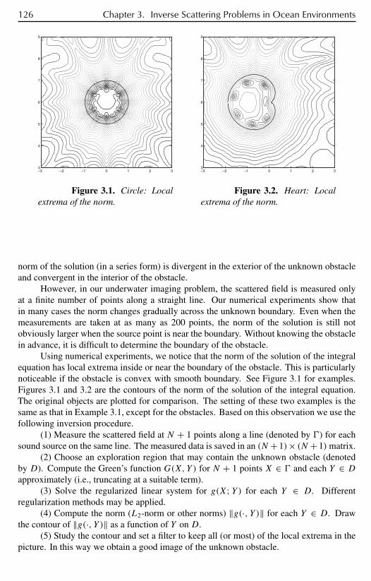
126 Chapter 3. Inverse Scattering Problems in Ocean Environments
–3 –2 –1 0 1 2 33
4
5
6
7
8
9
Figure 3.1. Circle: Localextrema of the norm.
–3 –2 –1 0 1 2 33
4
5
6
7
8
9
Figure 3.2. Heart: Localextrema of the norm.
norm of the solution (in a series form) is divergent in the exterior of the unknown obstacleand convergent in the interior of the obstacle.
However, in our underwater imaging problem, the scattered field is measured onlyat a finite number of points along a straight line. Our numerical experiments show thatin many cases the norm changes gradually across the unknown boundary. Even when themeasurements are taken at as many as 200 points, the norm of the solution is still notobviously larger when the source point is near the boundary. Without knowing the obstaclein advance, it is difficult to determine the boundary of the obstacle.
Using numerical experiments, we notice that the norm of the solution of the integralequation has local extrema inside or near the boundary of the obstacle. This is particularlynoticeable if the obstacle is convex with smooth boundary. See Figure 3.1 for examples.Figures 3.1 and 3.2 are the contours of the norm of the solution of the integral equation.The original objects are plotted for comparison. The setting of these two examples is thesame as that in Example 3.1, except for the obstacles. Based on this observation we use thefollowing inversion procedure.
(1) Measure the scattered field at N + 1 points along a line (denoted by ) for eachsound source on the same line. The measured data is saved in an (N +1)× (N +1)matrix.
(2) Choose an exploration region that may contain the unknown obstacle (denotedby D). Compute the Green’s function G(X, Y ) for N + 1 points X ∈ and each Y ∈ Dapproximately (i.e., truncating at a suitable term).
(3) Solve the regularized linear system for g(X;Y ) for each Y ∈ D. Differentregularization methods may be applied.
(4) Compute the norm (L2-norm or other norms) ‖g(·, Y )‖ for each Y ∈ D. Drawthe contour of ‖g(·, Y )‖ as a function of Y on D.
(5) Study the contour and set a filter to keep all (or most) of the local extrema in thepicture. In this way we obtain a good image of the unknown obstacle.
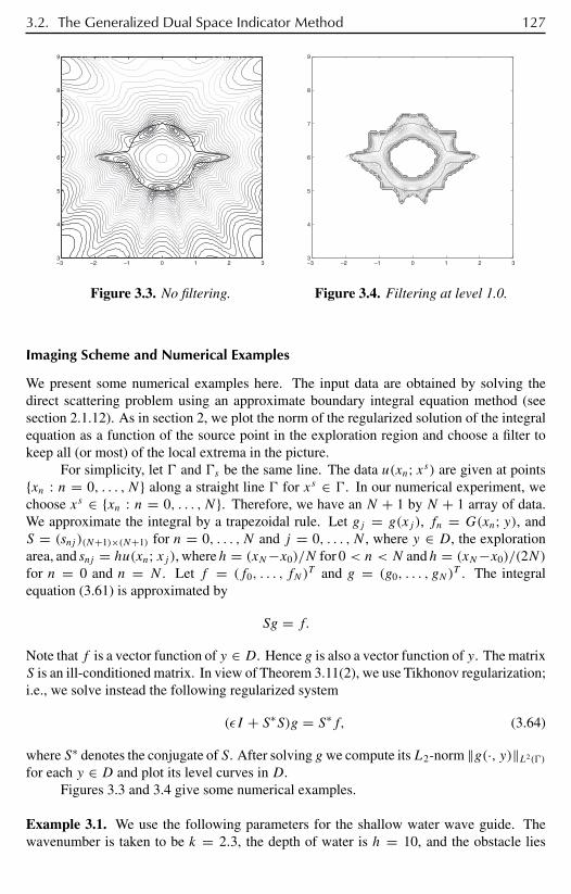
3.2. The Generalized Dual Space Indicator Method 127
–3 –2 –1 0 1 2 33
4
5
6
7
8
9
Figure 3.3. No filtering.
–3 –2 –1 0 1 2 33
4
5
6
7
8
9
Figure 3.4. Filtering at level 1.0.
Imaging Scheme and Numerical Examples
We present some numerical examples here. The input data are obtained by solving thedirect scattering problem using an approximate boundary integral equation method (seesection 2.1.12). As in section 2, we plot the norm of the regularized solution of the integralequation as a function of the source point in the exploration region and choose a filter tokeep all (or most) of the local extrema in the picture.
For simplicity, let and s be the same line. The data u(xn; xs) are given at pointsxn : n = 0, . . . , N along a straight line for xs ∈ . In our numerical experiment, wechoose xs ∈ xn : n = 0, . . . , N. Therefore, we have an N + 1 by N + 1 array of data.We approximate the integral by a trapezoidal rule. Let gj = g(xj ), fn = G(xn; y), andS = (snj )(N+1)×(N+1) for n = 0, . . . , N and j = 0, . . . , N , where y ∈ D, the explorationarea, and snj = hu(xn; xj ), whereh = (xN−x0)/N for 0 < n < N andh = (xN−x0)/(2N)for n = 0 and n = N . Let f = (f0, . . . , fN)
T and g = (g0, . . . , gN)T . The integral
equation (3.61) is approximated by
Sg = f.
Note that f is a vector function of y ∈ D. Hence g is also a vector function of y. The matrixS is an ill-conditioned matrix. In view of Theorem 3.11(2), we use Tikhonov regularization;i.e., we solve instead the following regularized system
(εI + S∗S)g = S∗f, (3.64)
where S∗ denotes the conjugate of S. After solving g we compute itsL2-norm ‖g(·, y)‖L2()
for each y ∈ D and plot its level curves in D.Figures 3.3 and 3.4 give some numerical examples.
Example 3.1. We use the following parameters for the shallow water wave guide. Thewavenumber is taken to be k = 2.3, the depth of water is h = 10, and the obstacle lies
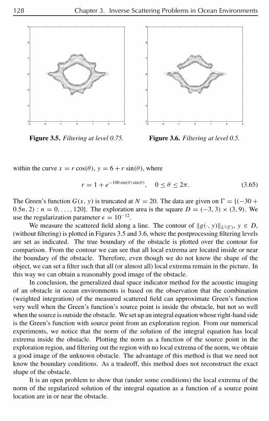
128 Chapter 3. Inverse Scattering Problems in Ocean Environments
–3 –2 –1 0 1 2 33
4
5
6
7
8
9
Figure 3.5. Filtering at level 0.75.
–3 –2 –1 0 1 2 33
4
5
6
7
8
9
Figure 3.6. Filtering at level 0.5.
within the curve x = r cos(θ), y = 6 + r sin(θ), where
r = 1 + e−100 sin(θ) sin(θ), 0 ≤ θ ≤ 2π. (3.65)
The Green’s function G(x, y) is truncated at N = 20. The data are given on = (−30 +0.5n, 2) : n = 0, . . . , 120. The exploration area is the square D = (−3, 3) × (3, 9). Weuse the regularization parameter ε = 10−12.
We measure the scattered field along a line. The contour of ‖g(·, y)‖L2(), y ∈ D,(without filtering) is plotted in Figures 3.5 and 3.6, where the postprocessing filtering levelsare set as indicated. The true boundary of the obstacle is plotted over the contour forcomparison. From the contour we can see that all local extrema are located inside or nearthe boundary of the obstacle. Therefore, even though we do not know the shape of theobject, we can set a filter such that all (or almost all) local extrema remain in the picture. Inthis way we can obtain a reasonably good image of the obstacle.
In conclusion, the generalized dual space indicator method for the acoustic imagingof an obstacle in ocean environments is based on the observation that the combination(weighted integration) of the measured scattered field can approximate Green’s functionvery well when the Green’s function’s source point is inside the obstacle, but not so wellwhen the source is outside the obstacle. We set up an integral equation whose right-hand sideis the Green’s function with source point from an exploration region. From our numericalexperiments, we notice that the norm of the solution of the integral equation has localextrema inside the obstacle. Plotting the norm as a function of the source point in theexploration region, and filtering out the region with no local extrema of the norm, we obtaina good image of the unknown obstacle. The advantage of this method is that we need notknow the boundary conditions. As a tradeoff, this method does not reconstruct the exactshape of the obstacle.
It is an open problem to show that (under some conditions) the local extrema of thenorm of the regularized solution of the integral equation as a function of a source pointlocation are in or near the obstacle.

3.3. Determination of an Inhomogeneity in a Two-Layered Wave Guide 129
3.3 Determination of an Inhomogeneity in a Two-LayeredWave Guide
Consider a 2D acoustic model of a two-layered wave guide:
M1 = (x, z)|0 < z < d,−∞ < x <∞,M2 = (x, z)|d < z < h,−∞ < x <∞, = (x, z)|z = d,−∞ < x <∞,
Rh2 = (x, z)|0 < z < h,−∞ < x <∞ = R × (0, h).Here d and h are constants, and h > d > 0.
We assume that the inhomogeneity is contained in a bounded domain with C2
boundary having an outward pointing normal vector. The propagating solution
u(x, z) = u1(x, z) if (x, z) ∈ M1 \,u2(x, z) if (x, z) ∈ M2,
u3(x, z) if (x, z) ∈ ,(3.66)
satisfies
u1 + k21u1 = −δ(x − xs)δ(z− zs) inM1 \, (3.67)
u3 + k23(x, z)u3 = 0 in , (3.68)
u2 + k22u2 = 0 inM2, (3.69)
ρ1u1 = ρ2u2 on , (3.70)
∂u1
∂ν= ∂u2
∂νon , (3.71)
u1 (x, 0) = 0, (3.72)
∂u2
∂z(x, h) = 0, (3.73)
ρ1u1 = ρ3u3 on ∂, (3.74)
∂u1
∂ν= ∂u3
∂νon ∂, (3.75)
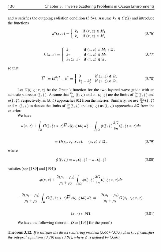
130 Chapter 3. Inverse Scattering Problems in Ocean Environments
and u satisfies the outgoing radiation condition (3.54). Assume k3 ∈ C() and introducethe functions
ko(x, z) =k1 if (x, z) ∈ M1,
k2 if (x, z) ∈ M2,(3.76)
k (x, z) =k1 if (x, z) ∈ M1 \,k2 if (x, z) ∈ M2
k3 (x, z) if (x, z) ∈ ,(3.77)
so that
k2 := (k0)2 − k2 =
0 if (x, z) /∈ ,k2
1 − k23 if (x, z) ∈ . (3.78)
Let G(ξ, ζ ; x, z) be the Green’s function for the two-layered wave guide with anacoustic source at (ξ, ζ ). Assume that ∂u−
∂n(ξ, ζ ) and u− (ξ, ζ ) are the limits of ∂u
∂n(ξ, ζ ) and
u(ξ, ζ ), respectively, as (ξ, ζ ) approaches ∂ from the interior. Similarly, we use ∂u+∂n(ξ, ζ )
and u+(ξ, ζ ) to denote the limits of ∂u∂n(ξ, ζ ) and u(ξ, ζ ) as (ξ, ζ ) approaches ∂ from the
exterior.We have
u(x, z)+∫
G(ξ, ζ ; x, z)k2u(ξ, ζ )dξ dζ −∫∂
φ(ξ, ζ )∂G
∂n(ξ, ζ ; x, z)ds
= G(xs, zs; x, z), (x, z) ∈ , (3.79)
where
φ(ξ, ζ ) = u+(ξ, ζ )− u−(ξ, ζ ) (3.80)
satisfies (see [189] and [194])
φ(x, z)+ 2(ρ1 − ρ3)
ρ1 + ρ3
∫∂
φ(ξ, ζ )∂G
∂n(ξ, ζ ; x, z)ds
−2(ρ1 − ρ3)
ρ1 + ρ3
∫
G(ξ, ζ ; x, z)k2u(ξ, ζ )dξ dζ = −2(ρ1 − ρ3)
ρ1 + ρ3G(xs, zs; x, z),
(x, z) ∈ ∂. (3.81)
We have the following theorem. (See [195] for the proof.)
Theorem 3.12. If u satisfies the direct scattering problem (3.66)–(3.75), then (u, φ) satisfiesthe integral equations (3.79) and (3.81), where φ is defined by (3.80).
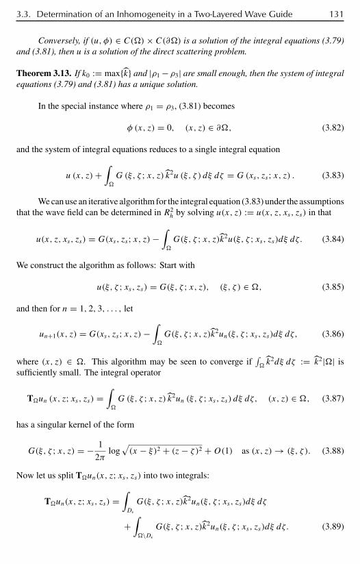
3.3. Determination of an Inhomogeneity in a Two-Layered Wave Guide 131
Conversely, if (u, φ) ∈ C()× C(∂) is a solution of the integral equations (3.79)and (3.81), then u is a solution of the direct scattering problem.
Theorem 3.13. If k0 := maxk and |ρ1 −ρ3| are small enough, then the system of integralequations (3.79) and (3.81) has a unique solution.
In the special instance where ρ1 = ρ3, (3.81) becomes
φ (x, z) = 0, (x, z) ∈ ∂, (3.82)
and the system of integral equations reduces to a single integral equation
u (x, z)+∫
G (ξ, ζ ; x, z) k2u (ξ, ζ ) dξ dζ = G(xs, zs; x, z) . (3.83)
We can use an iterative algorithm for the integral equation (3.83) under the assumptionsthat the wave field can be determined in R2
h by solving u(x, z) := u(x, z, xs, zs) in that
u(x, z, xs, zs) = G(xs, zs; x, z)−∫
G(ξ, ζ ; x, z)k2u(ξ, ζ ; xs, zs)dξ dζ. (3.84)
We construct the algorithm as follows: Start with
u(ξ, ζ ; xs, zs) = G(ξ, ζ ; x, z), (ξ, ζ ) ∈ , (3.85)
and then for n = 1, 2, 3, . . . , let
un+1(x, z) = G(xs, zs; x, z)−∫
G(ξ, ζ ; x, z)k2un(ξ, ζ ; xs, zs)dξ dζ, (3.86)
where (x, z) ∈ . This algorithm may be seen to converge if∫k2dξ dζ := k2|| is
sufficiently small. The integral operator
Tun (x, z; xs, zs) =∫
G (ξ, ζ ; x, z) k2un (ξ, ζ ; xs, zs) dξ dζ, (x, z) ∈ , (3.87)
has a singular kernel of the form
G(ξ, ζ ; x, z) = − 1
2πlog
√(x − ξ)2 + (z− ζ )2 +O(1) as (x, z)→ (ξ, ζ ). (3.88)
Now let us split Tun(x, z; xs, zs) into two integrals:
Tun(x, z; xs, zs) =∫Dε
G(ξ, ζ ; x, z)k2un(ξ, ζ ; xs, zs)dξ dζ
+∫\Dε
G(ξ, ζ ; x, z)k2un(ξ, ζ ; xs, zs)dξ dζ. (3.89)
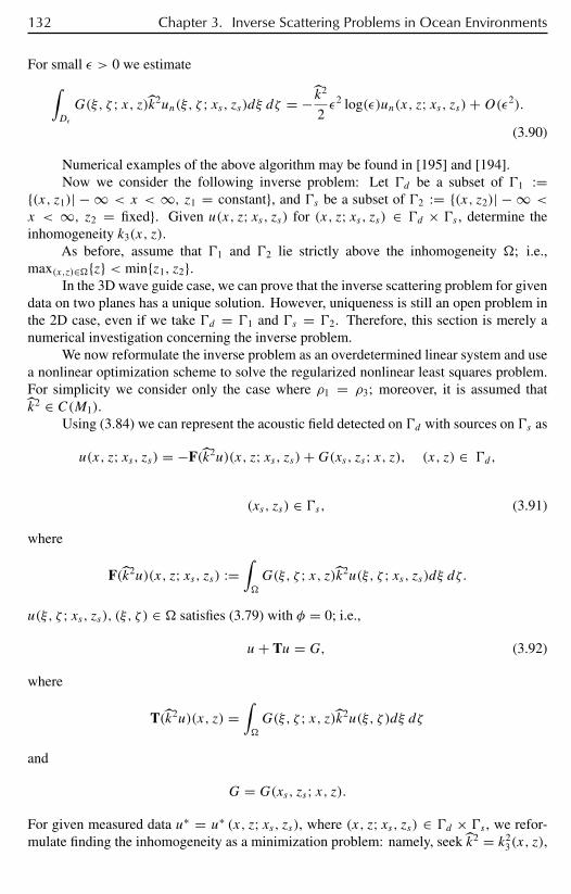
132 Chapter 3. Inverse Scattering Problems in Ocean Environments
For small ε > 0 we estimate∫Dε
G(ξ, ζ ; x, z)k2un(ξ, ζ ; xs, zs)dξ dζ = − k2
2ε2 log(ε)un(x, z; xs, zs)+O(ε2).
(3.90)
Numerical examples of the above algorithm may be found in [195] and [194].Now we consider the following inverse problem: Let d be a subset of 1 :=
(x, z1)| − ∞ < x < ∞, z1 = constant, and s be a subset of 2 := (x, z2)| − ∞ <
x < ∞, z2 = fixed. Given u(x, z; xs, zs) for (x, z; xs, zs) ∈ d × s , determine theinhomogeneity k3(x, z).
As before, assume that 1 and 2 lie strictly above the inhomogeneity ; i.e.,max(x,z)∈z < minz1, z2.
In the 3D wave guide case, we can prove that the inverse scattering problem for givendata on two planes has a unique solution. However, uniqueness is still an open problem inthe 2D case, even if we take d = 1 and s = 2. Therefore, this section is merely anumerical investigation concerning the inverse problem.
We now reformulate the inverse problem as an overdetermined linear system and usea nonlinear optimization scheme to solve the regularized nonlinear least squares problem.For simplicity we consider only the case where ρ1 = ρ3; moreover, it is assumed thatk2 ∈ C(M1).
Using (3.84) we can represent the acoustic field detected on d with sources on s as
u(x, z; xs, zs) = −F(k2u)(x, z; xs, zs)+G(xs, zs; x, z), (x, z) ∈ d,
(xs, zs) ∈ s, (3.91)
where
F(k2u)(x, z; xs, zs) :=∫
G(ξ, ζ ; x, z)k2u(ξ, ζ ; xs, zs)dξ dζ.
u(ξ, ζ ; xs, zs), (ξ, ζ ) ∈ satisfies (3.79) with φ = 0; i.e.,
u+ Tu = G, (3.92)
where
T(k2u)(x, z) =∫
G(ξ, ζ ; x, z)k2u(ξ, ζ )dξ dζ
and
G = G(xs, zs; x, z).For given measured data u∗ = u∗ (x, z; xs, zs), where (x, z; xs, zs) ∈ d × s , we refor-mulate finding the inhomogeneity as a minimization problem: namely, seek k2 = k2
3(x, z),

3.4. The Seamount Problem 133
(x, z) ∈ , such that the functional Jε (k2) is minimized for some suitably chosen ε. Herethe functional is defined by
Jε (k2) := ‖u∗ − F(k2(I + T)−1G)−G‖2L2(d )
+ ε‖ k2‖2L2(). (3.93)
Since max |k2| is small, we may approximate
(I + T)−1 ∼ I − T + T2 − T3,
which suggests solving the inverse problem by minimizing
Jε (k2) := ‖u∗ − F(k2(I − T + T2 − T3)G)−G‖2L2(d )
+ ε‖ k2‖2L2(). (3.94)
The difference between the minimization of (3.93) and the minimization of (3.94) is that nointegral equation needs to be solved in (3.94).
3.3.1 Numerical Example
We illustrate the method with a numerical example. The distributed inhomogeneity iscontained in a rectangle (x, z)|50 < x < 70, 75 < z < 90. The measured data are fromd = (−140 + 0.5m, 60)|m = 0, 1, 2, . . . , 800. The inhomogeneity is
k2 =
0.2sin( (z−77.5)π10 ) sin( (x−53.3)π
13.3 ), (x, z) ∈ [53.3, 66.6] × [77.5, 87.5],0 otherwise.
The reconstruction is shown in Figure 3.7.
3.4 The Seamount Problem
3.4.1 Formulation
In this section we continue to restrict our attention to constant depth oceans with completelyreflecting seabottoms. However, in the present example we consider the case where thereis a seamount on the ocean floor. We wish to reconstruct the seamount using far-fielddata. To this end we generate an acoustic field using a point source at a given location, say$x := (x1
0 , z0) = (x0, y0, z0). The acoustic pressure then satisfies
p + k2p = −δ($x − $x0), $x ∈ R3h \, (3.95)
p = 0 at z = h, (3.96)∂p
∂z= 0 at z = 0, a ≤ r ≤ ∞, (3.97)
∂p
∂ν= 0 on M, (3.98)
and the outgoing radiation condition. Here we assume that k = (2n+1)π2h , n = 0, 1, . . . , and
k2 is not an eigenvalue of the exterior boundary problem.
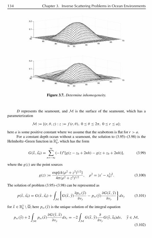
134 Chapter 3. Inverse Scattering Problems in Ocean Environments
5055
6065
70
7580
8590
0
0.1
0.2
5055
6065
70
7580
8590
0
0.1
0.2
Figure 3.7. Determine inhomogeneity.
D represents the seamount, and M is the surface of the seamount, which has aparameterization
M := (r, θ, z) : z := f (r, θ), 0 ≤ θ ≤ 2π, 0 ≤ r ≤ a;here a is some positive constant where we assume that the seabottom is flat for r > a.
For a constant depth ocean without a seamount, the solution to (3.95)–(3.98) is theHelmholtz–Green function in R3
h, which has the form
G($x, $x0) =∞∑
n=−∞(−1)n[g(z− z0 + 2nh)− g(z+ z0 + 2nh)], (3.99)
where the g(z) are the point sources
g(z) := expik(ρ2 + z2)1/24π(ρ2 + z2)1/2
, ρ2 = |x ′ − x10 |2. (3.100)
The solution of problem (3.95)–(3.98) can be represented as
p($x, $x0) = G($x, $x0)+∫
M
G($x, $y)∂psc($y)
∂νy− psc($y)∂G($x, $y)
∂νy
dsy (3.101)
for $x ∈ R3h \; here psc($y) is the unique solution of the integral equation
psc($y)+ 2∫
Mpsc($x)∂G($y, $x)
∂νydsx = −2
∫MG($x, $y) ∂
∂νyG($y, $x0)ds, $y ∈ M,
(3.102)
3.4. The Seamount Problem 135
and
∂
∂νpsc($y) = − ∂
∂νyG($y, $x0), $y ∈ M. (3.103)
The inverse problem is the following: Given p($x, $x0) for all $x ∈ , := (r, θ, z) :z = d = constant and $x0 ∈ 2, 2 := (r, θ, z) : z = d2 = constant, determine theseamount M.8
3.4.2 Uniqueness of the Seamount Problem
We assume that both 1 (the receiving plane) and 2 (the source location plane) are abovethe seamount. Our proof follows the uniqueness arguments for R3; in particular, see [261].
Theorem 3.14. Assume that D1 and D2 are two seamounts with rigid boundary M1 andM2 such that the corresponding solutions of problem (3.95)–(3.98) coincide on 1 for all$x0 ∈ , where is the unbounded component of R3
h (D1 ∪D2). Then D1 = D2.
Proof. Suppose that D1 = D2. Then without loss of generality we can assume there exists$x∗ ∈ ∂ such that $x∗ ∈ M1 and $x∗ /∈ M2. We choose ε > 0 such that
$xn := $x∗ + ε
nν($x∗) (n = 1, 2, . . . ) (3.104)
is contained in, where ν is the unit normal vector. Consider the solutionun,j to the problem(3.95)–(3.98) with $x0 replaced by $xn corresponding to the seamount Dj (j = 1, 2). Byassumption,
un,1 = un,2 on 1. (3.105)
In view of the fact that un,1 = un,2 = 0 at z = h and that un,j (j = 1, 2) are outgoing, weknow that un := un,1 − un,2 ≡ 0 in the region between 1 and the surface z = h. Owingto the real analyticity of solutions of the Helmholtz equation, it follows that un ≡ 0 in .Hence, un,1 = un,2 in . Consider un = un,2 as the wave corresponding to seamount D2.We know that the
∂un
∂ν= −∂G(·, $xn)
∂νon M2 (3.106)
are uniformly bounded with respect to the maximum norm on M2. It follows from thecontinuous dependence on the boundary values for the exterior Neumann problem that the∂un∂ν
are uniformly bounded with respect to the maximum norm on closed subsets of R3h\D2.
In particular, we have the estimate ∣∣∣∣∂un∂ν ($x∗)∣∣∣∣ ≤ C (3.107)
8Here we assume that 1 and 2 lie strictly above the seamount, i.e., maxr,θ z|z = f (r, θ) < mind1, d2.
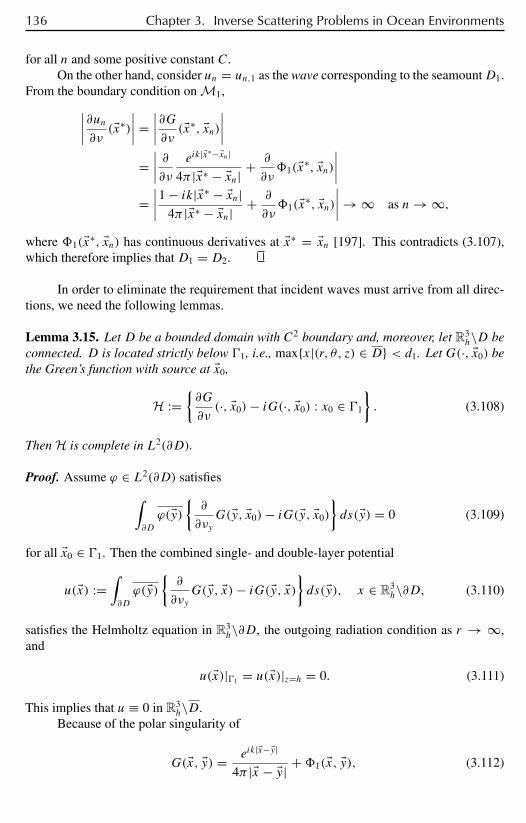
136 Chapter 3. Inverse Scattering Problems in Ocean Environments
for all n and some positive constant C.On the other hand, consider un = un,1 as the wave corresponding to the seamountD1.
From the boundary condition on M1,∣∣∣∣∂un∂ν ($x∗)∣∣∣∣ = ∣∣∣∣∂G∂ν ($x∗, $xn)
∣∣∣∣=∣∣∣∣ ∂∂ν eik|$x∗−$xn|
4π |$x∗ − $xn| + ∂
∂ν1($x∗, $xn)
∣∣∣∣=∣∣∣∣1 − ik|$x∗ − $xn|
4π |$x∗ − $xn| + ∂
∂ν1($x∗, $xn)
∣∣∣∣ → ∞ as n→ ∞,
where 1($x∗, $xn) has continuous derivatives at $x∗ = $xn [197]. This contradicts (3.107),which therefore implies that D1 = D2.
In order to eliminate the requirement that incident waves must arrive from all direc-tions, we need the following lemmas.
Lemma 3.15. Let D be a bounded domain with C2 boundary and, moreover, let R3h\D be
connected. D is located strictly below 1, i.e., maxx|(r, θ, z) ∈ D < d1. Let G(·, $x0) bethe Green’s function with source at $x0,
H :=∂G
∂ν(·, $x0)− iG(·, $x0) : x0 ∈ 1
. (3.108)
Then H is complete in L2(∂D).
Proof. Assume ϕ ∈ L2(∂D) satisfies∫∂D
ϕ($y)∂
∂νyG($y, $x0)− iG($y, $x0)
ds($y) = 0 (3.109)
for all $x0 ∈ 1. Then the combined single- and double-layer potential
u($x) :=∫∂D
ϕ($y)∂
∂νyG($y, $x)− iG($y, $x)
ds($y), x ∈ R3
h\∂D, (3.110)
satisfies the Helmholtz equation in R3h\∂D, the outgoing radiation condition as r → ∞,
and
u($x)|1 = u($x)|z=h = 0. (3.111)
This implies that u ≡ 0 in R3h\D.
Because of the polar singularity of
G($x, $y) = eik|$x−$y|
4π |$x − $y| +1($x, $y), (3.112)

3.4. The Seamount Problem 137
where 1($x, $y) is continuous at $x = $y, by letting $x → $y, we obtain the boundary integralequation
ϕ + Kϕ − iSϕ = 0 on ∂D. (3.113)
Here
Kϕ($x) : = 2∫∂D
∂G
∂νy($y, $x)ϕ($y)ds($y), (3.114)
Sϕ($x) : = 2∫∂D
G($y, $x)ϕ($y)ds($y). (3.115)
The operator I + K − iS is invertible for k = (2n+1)π2h (n = 0, 1, 2, . . . ) (see [197])
and its inverse is a bounded linear operator in L2(∂D). Hence, we have from (3.113) ϕ = 0on ∂D and the completeness of H is proved.
Lemma 3.16. Let D be a bounded domain with C2 boundary ∂D such that R3h\D is
connected andD is located strictly below 1. Let u ∈ C2(D)∩C1(D) be a solution of theHelmholtz equation. Then there exists a sequence vn in
V := spanG(·, $x0) : $x0 ∈ 1such that
vn → u, ∇vn → ∇u as n→ ∞, (3.116)
uniformly on compact subsets of D.
Proof. By Lemma 2.1, there exists a sequence vn in V such that∥∥∥∥∂vn∂v − ivn −(∂u
∂v− iu
)∥∥∥∥L2(∂D)
→ 0 as h→ ∞. (3.117)
Notice thatwn := un−u satisfies the Helmholtz equation inD and the impedance boundarycondition
∂wn
∂ν− iwn = ∂vn
∂ν− ivn −
(∂u
∂ν− iu
)on ∂D. (3.118)
We represent wn as a sequence of single-layer potentials
wn($x) :=∫∂D
G($y, $x)ψn($y)ds($y), $x ∈ D, n = 1, 2, . . . , (3.119)
where the ψn ∈ C(∂D) are density functions. Letting $x approach a point on ∂D, we obtainthe boundary integral equations
ψn + K′ψn − iS′ψn = 2fn on ∂D, (3.120)
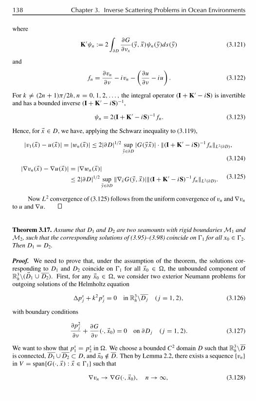
138 Chapter 3. Inverse Scattering Problems in Ocean Environments
where
K′ψn := 2∫∂D
∂G
∂νx($y, $x)ψn($y)ds($y) (3.121)
and
fn = ∂vn
∂ν− ivn −
(∂u
∂ν− iu
). (3.122)
For k = (2n + 1)π/2h, n = 0, 1, 2, . . . , the integral operator (I + K′ − iS) is invertibleand has a bounded inverse (I + K′ − iS)−1,
ψn = 2(I + K′ − iS)−1fn. (3.123)
Hence, for $x ∈ D, we have, applying the Schwarz inequality to (3.119),
|v1($x)− u($x)| = |wn($x)| ≤ 2|∂D|1/2 sup$y∈∂D
|G($y $x)| · ‖(I + K′ − iS)−1fn‖L2(∂D),
(3.124)
|∇vn($x)− ∇u($x)| = |∇wn($x)|≤ 2|∂D|1/2 sup
$y∈∂D‖∇$xG($y, $x)|‖(I + K′ − iS)−1fn‖L2(∂D).
(3.125)
NowL2 convergence of (3.125) follows from the uniform convergence of vn and ∇vnto u and ∇u.
Theorem 3.17. Assume that D1 and D2 are two seamounts with rigid boundaries M1 andM2, such that the corresponding solutions of (3.95)–(3.98) coincide on 1 for all x0 ∈ 2.Then D1 = D2.
Proof. We need to prove that, under the assumption of the theorem, the solutions cor-responding to D1 and D2 coincide on 1 for all $x0 ∈ , the unbounded component ofR3h\( $D1 ∪ D2). First, for any $x0 ∈ , we consider two exterior Neumann problems for
outgoing solutions of the Helmholtz equation
psj + k2psj = 0 in R3h\Dj (j = 1, 2), (3.126)
with boundary conditions
∂p2j
∂ν+ ∂G
∂ν(·, $x0) = 0 on ∂Dj (j = 1, 2). (3.127)
We want to show that ps1 = ps2 in . We choose a bounded C2 domain D such that R3h\D
is connected,D1 ∪D2 ⊂ D, and $x0 /∈ D. Then by Lemma 2.2, there exists a sequence vnin V = spanG(·, $x) : $x ∈ 1 such that
∇vn → ∇G(·, $x0), n→ ∞, (3.128)
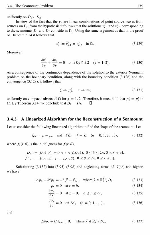
3.4. The Seamount Problem 139
uniformly on D1 ∪D2.
In view of the fact that the vn are linear combinations of point source waves fromsources on 1, from the hypothesis it follows that the solutions vsn,1 and vsn,2 correspondingto the seamounts D1 and D2 coincide in 1. Using the same argument as that in the proofof Theorem 3.14 it follows that
vsn := vsn,1 = vsn,2 in . (3.129)
Moreover,
∂vsn
∂ν+ ∂vn
∂ν= 0 on ∂Dj ∩ ∂ (j = 1, 2). (3.130)
As a consequence of the continuous dependence of the solution to the exterior Neumannproblem on the boundary condition, along with the boundary condition (3.126) and theconvergence (3.128), it follows that
vsn → psj , n→ ∞, (3.131)
uniformly on compact subsets of for j = 1, 2. Therefore, it must hold that ps1 = ps2 in. By Theorem 3.14, we conclude that D1 = D2.
3.4.3 A Linearized Algorithm for the Reconstruction of a Seamount
Let us consider the following linearized algorithm to find the shape of the seamount. Let
δpn = p − pn and δfn = f − fn (n = 0, 1, 2, . . . ), (3.132)
where f0(r, θ) is the initial guess for f (r, θ),
Dn : = (r, θ, z) := 0 < z < fn(r, θ), 0 ≤ θ ≤ 2π, 0 < r < a,Mn : = (r, θ, z) : z := fn(r, θ), 0 ≤ θ ≤ 2π, 0 ≤ r ≤ a.
Substituting (3.132) into (3.95)–(3.98) and neglecting terms of O(δ2) and higher,we have
pn + k2pn = −δ($x − $x0), where $x ∈ R3h \Dn, (3.133)
pn = 0 at z = h, (3.134)∂pn
∂z= 0 at z = 0, a ≤ r ≤ ∞, (3.135)
∂pn
∂ν= 0 on Mn (n = 0, 1, . . . ), (3.136)
and
δpn + k2δpn = 0, where $x ∈ R3h \Dn, (3.137)

140 Chapter 3. Inverse Scattering Problems in Ocean Environments
δpn = 0 at z = h, (3.138)∂δpn
∂z= 0 at z = 0, 0 ≤ r ≤ a, (3.139)
∂δpn
∂ν= −
(∂2
∂ν2pn
)δfn on Mn. (3.140)
We can now use single-layer potentials to obtain a relation between δpn and δfn in(3.140). Let us represent δpn as
δpn($x) :=∫
Mn
G ($x, $y) φ($y)dsy, $x ∈ R3h \Dn. (3.141)
Then φ($y) satisfies
φ($x)− 2∫
Mn
∂G ($x, $y)∂νx
φ($y)dsy = −2∂2
∂ν2pnδfn on Mn (3.142)
and ∫Mn
G ($x, $y) φ($y)dsy = δpn($x) := p($x)− pn($x) for $x ∈ 1. (3.143)
Now we can establish an iterative algorithm for solving the inverse problem as follows:
1. Initial guess f0(r, θ); for n = 0,2. Solve for pn($x) from (3.137)–(3.140).3. Let δpn($x) = p($x)− pn($x), Solve φ($y) = φn($y) for $y ∈ Mn from (3.143).4. For chosen εn > 0, set
δfn = min
εn,
[φ($x)− 2
∫Mn
∂G ($x, $y)∂νx
φ($y)dsy] [
−2∂2
∂ν2pn
]−1.
5. Let fn+1 = fn + δfn.Repeat steps 2–5 for (n = 1, 2, . . . ) solving forpn, δpn, φn, δfn, respectively, until |δfn| < εfor some chosen ε.
Step 3 in the above algorithm solves an ill-posed integral equation, inherited fromthe original ill-posedness of the inverse problem. A proper regularization method must beadapted in order to solve (3.143). With this in mind we first discuss some properties of theintegral operators T and TN defined by
Tφ($x) =∫
MG($x, $y)φ($y)dsy, $x ∈ 1, (3.144)
Tnφ($x) =∫
Mn
G($x, $y)φ($y)dsy, $x ∈ (n = 0, 1, 2, . . . ). (3.145)

3.4. The Seamount Problem 141
We will need the following spaces that are weighted in x ′ = (x1, x2) ∈ R2:
L2,s(R2) := u : (1 + |x ′|2)s/2u ∈ L2(R2)
,
H 1,s(R2) := u : Dαu ∈ L2,s(R2), |α| < 1
,
where we use the multi-index notation α = (α1, α2), |α| = |α1| + |α2|, and Dα = ∂α
∂xα11 ∂x
α22
;
L2 denotes the space of square-integrable functions, and L2(M), H 1(M), L2(Mn), andH 1(Mn) denote the usual Hilbert spaces and Sobolev spaces on the surfaces M and Mn,respectively.
Owing to the form of the normal mode expansion of the Helmholtz–Green functionG($x, $y),
G($x, $y) = i
4
∞∑n=0
∞∑m=−∞
εmφn(z)φn(z′)
‖φn‖2H(1)m (kanr)Jm(kanr
′) cos[m(θ − θ ′)], r ′ < r,
(3.146)
where $x = (r, θ, z), $y = (r ′, θ ′, z′) and an is purely imaginary except for a finite numberof ns, ε0 = 1, and εm = 2 for m = 0. We know that G($x, $y) is real analytic in $x for any$y ∈ M. Moreover, we have for some constant C the estimates
|G($x, $y)| < C|x ′|−1/2,
|DαG($x, $y)| < C|x ′|−1/2, |α| ≤ 2,
holding uniformly for $y ∈ M as |x ′| → ∞. From these facts we have the followingtheorem. (See [216] for proofs.)
Theorem 3.18.(1) The operator T is compact from L2(M) into H 1,−s(1) for s > 1/2.(2) The operator Tn is compact from L2(Mn) into H 1,−s(1) for s > 1/2.
Theorem 3.19. The operator T is injective and has dense range provided that the mixedboundary valued problem
u+ k2u = 0, $x ∈ D, (3.147)
u = 0 on M, (3.148)
∂u
∂z= 0 at z = 0, 0 ≤ r ≤ a, (3.149)
has no nontrivial solution.
Based on Theorems 3.18 and 3.19, we may apply the Tikhonov regularization tostep 3; that is, we solve
αφα + T∗nTnφα = T∗
n(p − pn) (3.150)
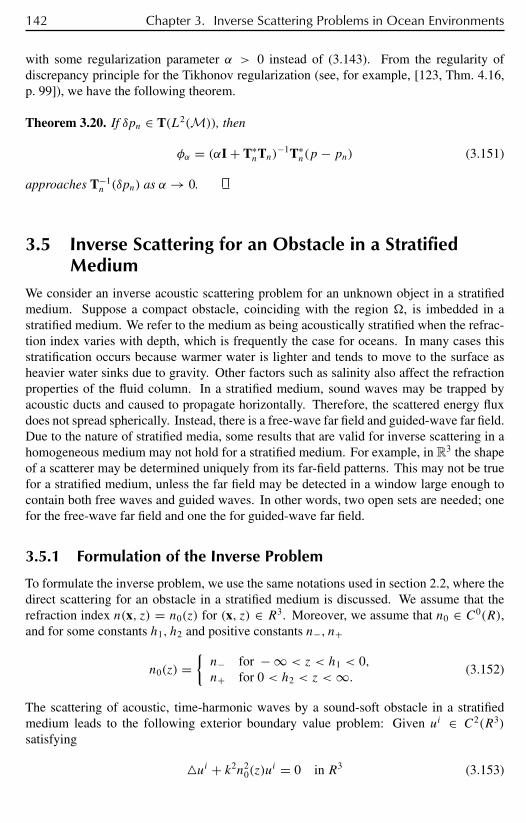
142 Chapter 3. Inverse Scattering Problems in Ocean Environments
with some regularization parameter α > 0 instead of (3.143). From the regularity ofdiscrepancy principle for the Tikhonov regularization (see, for example, [123, Thm. 4.16,p. 99]), we have the following theorem.
Theorem 3.20. If δpn ∈ T(L2(M)), then
φα = (αI + T∗nTn)
−1T∗n(p − pn) (3.151)
approaches T−1n (δpn) as α → 0.
3.5 Inverse Scattering for an Obstacle in a StratifiedMedium
We consider an inverse acoustic scattering problem for an unknown object in a stratifiedmedium. Suppose a compact obstacle, coinciding with the region , is imbedded in astratified medium. We refer to the medium as being acoustically stratified when the refrac-tion index varies with depth, which is frequently the case for oceans. In many cases thisstratification occurs because warmer water is lighter and tends to move to the surface asheavier water sinks due to gravity. Other factors such as salinity also affect the refractionproperties of the fluid column. In a stratified medium, sound waves may be trapped byacoustic ducts and caused to propagate horizontally. Therefore, the scattered energy fluxdoes not spread spherically. Instead, there is a free-wave far field and guided-wave far field.Due to the nature of stratified media, some results that are valid for inverse scattering in ahomogeneous medium may not hold for a stratified medium. For example, in R3 the shapeof a scatterer may be determined uniquely from its far-field patterns. This may not be truefor a stratified medium, unless the far field may be detected in a window large enough tocontain both free waves and guided waves. In other words, two open sets are needed; onefor the free-wave far field and one the for guided-wave far field.
3.5.1 Formulation of the Inverse Problem
To formulate the inverse problem, we use the same notations used in section 2.2, where thedirect scattering for an obstacle in a stratified medium is discussed. We assume that therefraction index n(x, z) = n0(z) for (x, z) ∈ R3. Moreover, we assume that n0 ∈ C0(R),and for some constants h1, h2 and positive constants n−, n+
n0(z) =n− for − ∞ < z < h1 < 0,n+ for 0 < h2 < z <∞. (3.152)
The scattering of acoustic, time-harmonic waves by a sound-soft obstacle in a stratifiedmedium leads to the following exterior boundary value problem: Given ui ∈ C2(R3)
satisfying
ui + k2n20(z)u
i = 0 in R3 (3.153)
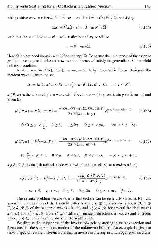
3.5. Inverse Scattering for an Obstacle in a Stratified Medium 143
with positive wavenumber k, find the scattered field us ∈ C2(R3 \) satisfying
us + k2n20(z)u
s = 0 in R3 \ (3.154)
such that the total field u = ui + us satisfies boundary condition
u = 0 on ∂. (3.155)
Here is a bounded domain withC2 boundary ∂. To ensure the uniqueness of the exteriorproblem, we require that the unknown scattered wave us satisfy the generalized Sommerfeldradiation condition.
As discussed in [469], [473], we are particularly interested in the scattering of theincident wave ui from the set
U := ui(·;α)|α ∈ S1 ∪ uij (·; α, β)|(α, β) ∈ D1, 1 ≤ j ≤ N.
ui(P ;α) is the distorted plane wave with direction α = (sin γ cos δ, sin γ sin δ, cos γ ) andgiven by
ui(P ;α) = F 0f (−α;P) = −ikn+ cos γp1(z, kn+ sin γ )
2πW(kn+ sin γ )eikn+r sin γ cos(δ−θ) (3.156)
for 0 ≤ γ < π
2, 0 ≤ δ, θ ≤ 2π, 0 ≤ r <∞, −∞ < z < +∞,
ui(P ;α) = F 0f (−α;P) = −ikn− cos γp2(z, kn− sin γ )
2πW(kn− sin γ )eikn−r sin γ cos(δ−θ) (3.157)
forπ
2< γ ≤ π, 0 ≤ δ, θ ≤ 2π, 0 ≤ r <∞, −∞ < z < +∞.
uij (P ; α, β) is the j th normal mode wave with direction (α, β) = (cos δ, sin δ, β),
uij (P ; α, β) = F 0g (−α, β;P ; j) =
√kaj
2πi
φj (β)φj (z)
W ′(kaj )eikaj r cos(δ−θ), (3.158)
−∞ < β, ζ <∞, 0 ≤ δ, θ ≤ 2π, 0 ≤ r <∞, j ∈ IN .The inverse problem we consider in this section can be generally stated as follows:
given the combination of the far-field patterns Ff (·;α) ⊕ Fg(·;α) and Ff (·; α, β; j) ⊕Fg(·; α, β; j) of the scattered waves us(·;α) and usj (·; α, β) for several incident wavesui(·;α) and uij (·; α, β) from U with different incident directions α, (α, β) and differentmodes j ∈ IN , determine the shape of the scatterer .
We discuss the uniqueness of the inverse obstacle scattering in the next section andthen consider the shape reconstruction of the unknown obstacle. An example is given toshow a special feature different from that in inverse scattering in a homogeneous medium.
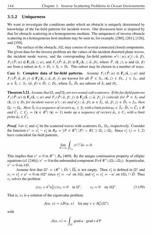
144 Chapter 3. Inverse Scattering Problems in Ocean Environments
3.5.2 Uniqueness
We want to investigate the conditions under which an obstacle is uniquely determined byknowledge of the far-field patterns for incident waves. Our discussion here is inspired bythat for obstacle scattering in a homogeneous medium. The uniqueness of inverse obstaclescattering in a homogeneous host medium may be seen in, for example, [280], [261], [126],and [350].
The surface of the obstacle, ∂, may consist of several connected closed components.The given data for the inverse problem are the values of the incident distorted plane waves,the incident mode waves, and the corresponding far-field patterns ui(·;α), uij (·; α, β),Ff (P ;α) ⊕ Fg(x, z;α), and Ff (P ; α, β) ⊕ Fg(x, z; α, β), where P , (x, z), α and (α, β)are from a subset in S1 ×D1 × S1 ×D1. This subset may be chosen in a number of ways.
Case 1: Complete data of far-field patterns. Assume Ff (P ;α) ⊕ Fg(x, z;α) andFf (P ; α, β; j) ⊕ Fg(x, z; α, β; j) are known for all P ∈ S1, (x, z) ∈ D1, j ∈ IN , andα ∈ S1 ⊂ S1, (α, β) ∈ D1 ⊂ D1, where S1, D1 are subsets of S1 and D1.
Theorem 3.21. Assume that1 and2 are two sound-soft scatterers. If the far-field patternsFf (P ;α) ⊕ Fg(x, z;α) and Ff (P ; α, β; j) ⊕ Fg(x, z; α, β; j) coincide for P ∈ S1 and(x, z) ∈ D1 for incident waves ui(·;α) and uij (·; α, β), α ∈ S1, (α, β; j) ∈ D1 × IN , then
1 = 2. Here S1 is a sequence of vectors αn ∈ S1 with a limit point α0 ∈ S1; D1 = C1 ×Rand C1 ⊂ C1 = x ∈ R2| |x| = 1 make up a sequence of vectors αn ∈ C1 with a limitpoint α0 ∈ C1.
Proof. Let vs1 and vs2 be the scattered waves with scatterers 1, 2, respectively. Considerthe function vs = vs1 − vs2 in BR = P ∈ R3| |P | < R ⊃ 1 ∪ 2. Since vsj (j = 1, 2)have coincident far-field patterns,
limR→∞
∫R
|vs |2ds = 0.
This implies that vs = 0 in R3 \ BR [469]. By the unique continuation property of ellipticequations (cf. [246]), vs = 0 in the unbounded componentD ofR3\(1∪2). In particular,vs = 0 on ∂D.
Assume first that ∗ = (R3 \ D) \ 2 is not empty. Then vs2 is defined in ∗ andv2 = vs2 + ui = 0 on ∂∗ since vs2 = −ui on ∂2 and vs2 = vs1 = −ui on ∂1 ∩ D. Thusv2 solves the problem
v2 + k2n20(z)v2 = 0 in ∗, v2 = 0 on ∂∗. (3.159)
That is, v2 is a solution of the eigenvalue problem
A(u, v) = λB(u, v) for any v ∈ H 10 (
∗)
with
A(u, v) =∫∗
grad u · grad v dP
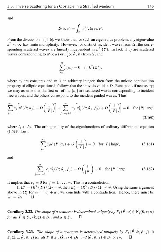
3.5. Inverse Scattering for an Obstacle in a Stratified Medium 145
and
B(u, v) =∫∗n2
0(z)uv dP.
From the discussion in [446], we know that for such an eigenvalue problem, any eigenvaluek2 < ∞ has finite multiplicity. However, for distinct incident waves from U , the corre-sponding scattered waves are linearly independent in L2(∗). In fact, if vj are scatteredwaves corresponding to ui(·;α) or uij (·; α, β) from U , and
m∑j=1
cjvj = 0 in L2(∗),
where cj are constants and m is an arbitrary integer, then from the unique continuationproperty of elliptic equations it follows that the above is valid inD. Rename vj if necessary;we may assume that the first m1 of the vj are scattered waves corresponding to incidentfree waves, and the others correspond to the incident guided waves. Thus,
m1∑j=1
cj
[ui(P ;αj )+O
(1
|P |)]
+m∑
j=m1+1
cj
[uilj (P ; αj , βj )+O
(1
|P |)]
= 0 for |P | large,
(3.160)
where lj ∈ IN . The orthogonality of the eigenfunctions of ordinary differential equation(1.5) follows:
m1∑j=1
cjui(P ;αj )+O
(1
|P |)
= 0 for |P | large, (3.161)
and
m∑j=m1+1
cjuilj(P ; αj , βj )+O
(1
|P |)
= 0 for |P | large. (3.162)
It implies that cj = 0 for j = 1, . . . , m. This is a contradiction.If∗ = (R3 \ D) \ 2 = ∅, then∗
1 = (R3 \ D) \ 1 = ∅. Using the same argumentabove in ∗
1 for v1 = vs1 + ui , we conclude with a contradiction. Hence, there must be1 = 2.
Corollary 3.22. The shape of a scatterer is determined uniquely by Ff (P ;α)⊕Fg(x, z;α)for all P ∈ S1, (x, z) ∈ D1, and α ∈ S1.
Corollary 3.23. The shape of a scatterer is determined uniquely by Ff (P ; α, β; j) ⊕Fg(x, z; α, β; j) for all P ∈ S1, (x, z) ∈ D1, and (α, β; j) ∈ D1 × IN .
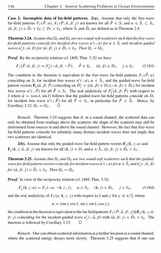
146 Chapter 3. Inverse Scattering Problems in Ocean Environments
Case 2: Incomplete data of far-field patterns. 2(a). Assume that only the free-wavefar-field patterns Ff (P ;α), Ff (P ; α, β; j) are known for all P ∈ S1 and α ∈ S1 ⊂ S1,(α, β; j) ∈ D1 × IN ⊂ D1 × IN , where S1 and D1 are defined as in Theorem 2.4.
Theorem 3.24. Assume that1 and2 are two sound-soft scatterers such that the free-wavefar-field patterns coincide for incident free waves ui(·;α) for α ∈ S1 and incident guidedwaves uij (·; α, β) for (α, β; j) ∈ D1 × IN . Then 1 = 2.
Proof. By the reciprocity relation (cf. [469, Thm. 3.3]) we have
Ff (P ; α, β; j) = Fjg (−α, β;−P ), P ∈ S1, (α, β) ∈ D1, j ∈ IN . (3.163)
The condition in the theorem is equivalent to the free-wave far-field patterns Ff (P ;α)coinciding on S1 for incident free waves ui(·;α), α ∈ S1, and the guided-wave far-fieldpattern vectors Fg(α, β; P ) coinciding on D∗
1 = (α, β) ∈ D1|(−α, β) ∈ D1 for incidentfree waves ui(·; P ) for all P ∈ S1. The real analyticity of Fjg (α, β; P ) with respect toδ where α = (cos δ, sin δ) follows that the guided-wave far-field patterns coincide on D1
for incident free wave ui(·; P ) for all P ∈ S1, in particular for P ∈ S1. Hence, byCorollary 3.23, 1 = 2.
Remark. Theorem 3.24 suggests that if, in a sound channel, the scattered data canonly be obtained from readings above the scatterer, the shape of the scatterer may still bedetermined from sources in and above the sound channel. However, the fact that free-wavefar-field patterns coincide for infinitely many distinct incident waves does not imply thattwo scatterers are identical.
2(b). Assume that only the guided-wave far-field pattern vectors Fg(x, z;α) andFg(x, z; α, β; j) are known for all (x, z) ∈ D1 and α ∈ S1, (α, β; j) ∈ D1 × IN .
Theorem 3.25. Assume that1 and2 are two sound-soft scatterers such that the guided-wave far-field pattern vectors coincide for incident waves ui(·;α) for α ∈ S1 and uij (·; α, β)for (α, β; j) ∈ D1 × IN . Then 1 = 2.
Proof. In view of the reciprocity relation (cf. [469, Thm. 3.3])
F jg (x, z;α) = Ff (−α;−x, z; j), α ∈ S1, (x, z) ∈ D1, j ∈ IN, (3.164)
and the real analyticity of Ff (α; x, z; j) with respect to δ and γ for γ = π/2, where
α = (sin γ cos δ, sin γ sin δ, cos γ ),
the condition in the theorem is equivalent to the far-field patternsFf (P ; α, β; j)⊕Fg(x, z; α,β; j) coinciding for the incident guided wave uij (·; α, β) with (α, β; j) ∈ D1 × IN . Thetheorem is followed by Corollary 3.23.
Remark. One can obtain scattered information at a further location in a sound channel,where the scattered energy decays more slowly. Theorem 3.25 suggests that if one can
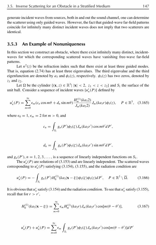
3.5. Inverse Scattering for an Obstacle in a Stratified Medium 147
generate incident waves from sources, both in and out the sound channel, one can determinethe scatterer using only guided waves. However, the fact that guided-wave far-field patternscoincide for infinitely many distinct incident waves does not imply that two scatterers areidentical.
3.5.3 An Example of Nonuniqueness
In this section we construct an obstacle, where there exist infinitely many distinct, incident-waves for which the corresponding scattered waves have vanishing free-wave far-fieldpatterns.
Let n2(z) be the refraction index such that there exist at least three guided modes.That is, equation (2.74) has at least three eigenvalues. The third eigenvalue and the thirdeigenfunction are denoted by a3 and φ3(z), respectively. φ3(z) has two zeros, denoted byz1 and z2.
Let be the cylinder (x, z) ∈ R3| |x| < 2, z1 < z < z2 and S1 the surface of theunit ball. Consider a sequence of incident waves uin(P ) defined by
uin(P ) =∞∑m=0
εm(cn cosmθ + dn sinmθ)H(1)m (ka32)
Jm(ka32)Jm(ka3r)φ3(z), P ∈ R3, (3.165)
where ε0 = 1, εm = 2 for m > 0, and
cn =∫S1
gn(P′)φ3(ζ )Jm(ka3r
′) cosmθ ′dP ′,
dn =∫S1
gn(P′)φ3(ζ )Jm(ka3r
′) sinmθ ′dP ′,
and gn(P ′), n = 1, 2, 3, . . . , is a sequence of linearly independent functions on S1.The uin(P ) are solutions of (3.153) and are linearly independent. The scattered waves
corresponding to uin(P ) satisfying (3.154), (3.155), and the radiation condition are
usn(P ) = −∫S1
gn(P′)H (1)
0 (ka3|x − ξ |)φ3(ζ )φ3(z)dP′, P ∈ R3 \. (3.166)
It is obvious that usn satisfy (3.154) and the radiation condition. To see that usn satisfy (3.155),recall that for r > r ′,
H(1)0 (ka3|x − ξ |) =
∞∑m=0
εmH(1)m (ka3r)Jm(ka3r
′) cos[m(θ − θ ′)], (3.167)
uin(P )+ usn(P ) =∞∑m=0
εm
∫S1
gn(P′)φ3(ζ )Jm(ka3r
′) cos[m(θ − θ ′)]dP ′
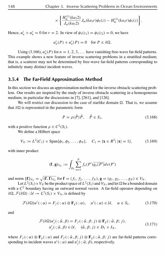
148 Chapter 3. Inverse Scattering Problems in Ocean Environments
×H(1)m (ka32)
Jm(ka32)Jm(ka3r)φ3(z)−H(1)
m (ka3r)φ3(z)
.
Hence, uin + usn = 0 for r = 2. In view of φ3(z1) = φ3(z2) = 0, we have
uin(P )+ usn(P ) = 0 for P ∈ ∂.Using (3.166), usn(P ) for n = 1, 2, 3, . . . have vanishing free-wave far-field patterns.
This example shows a new feature of inverse scattering problems in a stratified medium;that is, a scatterer may not be determined by free-wave far-field patterns corresponding toinfinitely many distinct incident waves.
3.5.4 The Far-Field Approximation Method
In this section we discuss an approximation method for the inverse obstacle scattering prob-lem. Our results are inspired by the study of inverse obstacle scattering in a homogeneousmedium, in particular the discussions in [7], [261], and [126].
We will restrict our discussion to the case of starlike domain . That is, we assumethat ∂ is represented in the parametric form
P = ρ(P )P , P ∈ S1, (3.168)
with a positive function ρ ∈ C2(S1).We define a Hilbert space
VN := L2(C1)× Spanφ1, φ2, . . . , φN , C1 = x ∈ R2| |x| = 1, (3.169)
with inner product
(f , g)VN :=∫D1
N∑n=1
fn(P′)gn(P ′)ds(P ′)
and norm ‖f‖VN = √(f , f)VN for f = (f1, f2, . . . , fN), g = (g1, g2, . . . , gN) ∈ VN .
LetL2(S1)×VN be the product space ofL2(S1) andVN , and let be a bounded domainwith a C2 boundary having an outward normal vector. A far-field operator depending on∂, F(∂) : U → L2(S1)× VN , is defined by
F(∂)ui(·;α) = Ff (·;α)⊕ Fg(·;α), ui(·;α) ∈ U, α ∈ S1, (3.170)
and
F(∂)uij (·; α, β) = Ff (·; α, β; j)⊕ Fg(·; α, β; j),uij (·; α, β) ∈ U, (α, β; j) ∈ D1 × IN, (3.171)
where Ff (·;α) ⊕ Fg(·;α) and Ff (·; α, β; j) ⊕ Fg(·; α, β; j) are far-field patterns corre-sponding to incident waves ui(·;α) and uij (·; α, β), respectively.

3.5. Inverse Scattering for an Obstacle in a Stratified Medium 149
Let B be the set of all starlike boundaries and W the set of all far-field operators.By the uniqueness theorem in section 3.5.2, the mapping ∂ &→ F(∂) is a one-to-onemapping from B to W .
Define integral operators K, S by
(Kφ)(P ) := 2∫∂
∂G(P ;P ′)∂ν(P ′)
φ(P ′)ds(P ′), P ∈ ∂,
(Sφ)(P ) := 2∫∂
G(P ;P ′)φ(P ′)ds(P ′), P ∈ ∂.
It is easy to prove that for any λ = 0, the operatorK+ iλS : C(∂)→ C(∂) is compact.
Theorem 3.26. Let be a bounded domain with aC2 boundary having an outward normalvector. The far-field operator depending on ∂ has representation
F(∂)ui(P ;α) = −2∫∂
(∂
∂ν+ iλ
)F 0f (P ;P ′)
⊕ F0g(x, z;P ′)(I +K + iλS)−1ui(P ′;α)ds(P ′) (3.172)
F(∂)uij (P ; α, β) = −2∫∂
(∂
∂ν+ iλ
)F 0f (P ;P ′)
⊕ F0g(x, z;P ′)(I +K + iλS)−1uij (P
′; α, β)ds(P ′) (3.173)
for any ui(·;α) and uij (·; α, β) ∈ U .
Proof. As discussed in [469], we can write us(P ;α) in the form
us(P ) =∫∂
[∂G
∂ν(P ;P ′)+ iλG(P ;P ′)
]φ(P ′)ds(P ′), P /∈ ∂, (3.174)
where φ ∈ C(∂). Then φ satisfies
φ + (K + iλS)φ = −2ui on ∂. (3.175)
Equation (3.175) has a unique solution for any ui ∈ U , and the operator I + K + λS hasbounded inverse operator (I +K + λS)−1 in C(∂). Hence
φ = (I +K + λS)−1(−2ui)
and
us(P ) = −2∫∂
[∂G
∂ν(P ;P ′)+ iλG(P ;P ′)
](I +K + λS)−1ui(P ′)ds(P ′).
Using the asymptotic representation of the Green’s function (cf. [469], [473])
G(P ;P ′) = eikR
RF 0f (θ, φ;P ′)+ 1√
rAg(r) · F0
g(θ, z;P ′)+ R0f (P )+ R0
g(P ), (3.176)

150 Chapter 3. Inverse Scattering Problems in Ocean Environments
we have
Ff (P ) = −2∫∂
[∂
∂ν+ iλ
]F 0f (P ;P ′)(I +K + λS)−1ui(P ′)ds(P ′),
Fg(x; z) = −2∫∂
[∂
∂ν+ iλ
]F0g(x, z;P ′)(I +K + λS)−1ui(P ′)ds(P ′).
The theorem is implied.
Following Angell, Colton, and Kirsch [7], we consider the following continuousdependence on boundary. Letn, be a sequence of starlike C2 surfaces having represen-tation
Pn = ρn(P )P , P = ρ(P )P , P ∈ S1.
By the convergence n → , n → ∞, we mean the convergence ‖ρn − ρ‖1,µ → 0,n → ∞, where ‖ · ‖1,µ is the C1,µ Hölder norm on S1. A sequence of function fn fromL2(n) is L2 convergent to a function f in L2() if
limn→∞
∫S1
|fn(ρn(P )P )− f (ρ(P )P )|2ds(P ) = 0.
Theorem 3.27. Letn be a sequence of starlike C2 surfaces that converges with respect tothe C1,µ norm to a C2 surface as n→ ∞, and let un and u be solutions to the Helmholtzequation in the exterior of n and , respectively. Assume that the continuous boundaryvalues of un onn are L2 convergent to the boundary values of u on. Then the sequenceun, together with all its derivatives, converges to u uniformly on compact subsets of theopen exterior of .
Proof. Representing u in the form of the combined double- and single-layer potential(3.174), and using (3.175), we obtain
ψ(P )+∫S1
H(P ; P ′)ψ(P ′)ds(P ′) = f (P ), P ∈ S1, (3.177)
where ψ(P ) = φ(ρ(P )P ), f (P ) = −2ui(ρ(P )P ),
H(P ; P ′) = 2
∂
∂ν(P ′)G(P ; P ′)+ iλG(P ; P ′)
J(P
′), (3.178)
P = ρ(P )P , P ′ = ρ(P ′)P ′,
G(P ; P ′) = G(ρ(P )P , ρ(P ′)P ′),

3.5. Inverse Scattering for an Obstacle in a Stratified Medium 151
JR(P′) = ρ(P
′)√
|ρ(P )|2 + | ρ(P )|2. (3.179)
Writing
G(P ;P ′) = (P ;P ′)+G1(P ;P ′),
where
(P ;P ′) = eikn(z)|P−P ′|
4π |P − P ′|and G1 ∈ C2(R3 \ P ), we have
H(P ; P ′) = 2
∂
∂ν(P ′)(P ; P ′)+ iλ(P ; P ′)
JR(P
′)
+ 2
∂
∂ν(P ′)G1(P ; P ′)+ iλG1(P ; P ′)
JR(P
′)
= 2
ν(P ′) · (P − P ′)
c1(|P − P ′|)|P − P ′|3 + c2(|P − P ′|)
|P − P ′| + c3(|P − P ′|)JR(P ),
where c1, c2, and c3 are C1 functions. Using the inequalities proved by Angell, Colton,and Kirsch (cf. [7] or [126, Lemmas 5.10 and 5.11]), we can prove that if R,Q ∈ C1,µ(S1)
and R(P ),Q(P ) ≥ a for some positive constant a, then there exist constants M > 0 and0 < µ1, µ2 < 1, such that
|HR(P ; P ′)| ≤ M
|P − P ′|2−µ2,
|HR(P ; P ′)−HQ(P ; P ′)| ≤ M‖R −Q‖µ11−µ
|P − P ′|2−µ2
for all P , P ′ ∈ S1. Proceeding along the line of the proof of [126, Thm. 5.9], we prove thetheorem.
Theorem 3.28.(1) The far-field operator F(∂) is injective.(2) Let F1(∂) := F(∂) (I +K + λS) : L2(∂)→ L2(S1)× VN .
F1(∂) has a dense range in L2(S1)× VN . Moreover, if k2 is not the Dirichlet eigenvaluefor (2.2) in , then the range of F(∂) consists of a complete set in L2(S1)× VN .
Proof. (1) Let F(∂)ui1 = F(∂)ui2 and φ = −2(I +K + iλS)−1(ui1 − ui2). Then
F1(∂)φ =∫∂
(∂
∂ν+ iλ
)F 0f ⊕ F0
gφds = 0,
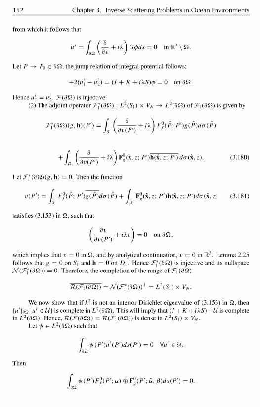
152 Chapter 3. Inverse Scattering Problems in Ocean Environments
from which it follows that
us =∫∂
(∂
∂ν+ iλ
)Gφds = 0 in R3 \.
Let P → P0 ∈ ∂; the jump relation of integral potential follows:
−2(ui1 − ui2) = (I +K + iλS)φ = 0 on ∂.
Hence ui1 = ui2. F(∂) is injective.(2) The adjoint operator F∗
1 (∂) : L2(S1)× VN → L2(∂) of F1(∂) is given by
F∗1 (∂)(g, h)(P
′) =∫S1
(∂
∂ν(P ′)+ iλ
)F 0f (P ;P ′)g(P )dσ (P )
+∫D1
(∂
∂ν(P ′)+ iλ
)F0g(x, z;P ′)h(x, z;P ′) dσ (x, z). (3.180)
Let F∗1 (∂)(g, h) = 0. Then the function
v(P ′) =∫S1
F 0f (P ;P ′)g(P )dσ (P )+
∫D1
F0g(x, z;P ′)h(x, z;P ′)dσ (x, z) (3.181)
satisfies (3.153) in , such that(∂v
∂ν(P ′)+ iλv
)= 0 on ∂,
which implies that v = 0 in , and by analytical continuation, v = 0 in R3. Lemma 2.25follows that g = 0 on S1 and h = 0 on D1. Hence F∗
1 (∂) is injective and its nullspaceN (F∗
1 (∂)) = 0. Therefore, the completion of the range of F1(∂)
R(F1(∂)) = N (F∗1 (∂))
⊥ = L2(S1)× VN.
We now show that if k2 is not an interior Dirichlet eigenvalue of (3.153) in , thenui |∂| ui ∈ U is complete in L2(∂). This will imply that (I +K+ iλS)−1U is completein L2(∂). Hence, R(F(∂)) = R(F1(∂)) is dense in L2(S1)× VN .
Let ψ ∈ L2(∂) such that∫∂
ψ(P ′)ui(P ′)ds(P ′) = 0 ∀ui ∈ U .
Then ∫∂
ψ(P ′)F 0f (P
′;α)⊕ F0g(P
′; α, β)ds(P ′) = 0.
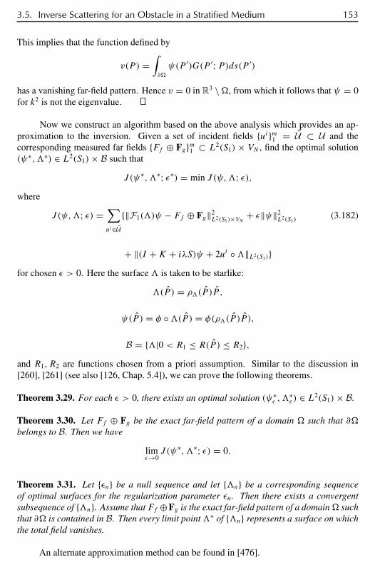
3.5. Inverse Scattering for an Obstacle in a Stratified Medium 153
This implies that the function defined by
v(P ) =∫∂
ψ(P ′)G(P ′;P)ds(P ′)
has a vanishing far-field pattern. Hence v = 0 in R3 \, from which it follows that ψ = 0for k2 is not the eigenvalue.
Now we construct an algorithm based on the above analysis which provides an ap-proximation to the inversion. Given a set of incident fields uim1 = U ⊂ U and thecorresponding measured far fields Ff ⊕ Fgm1 ⊂ L2(S1) × VN , find the optimal solution(ψ∗,∗) ∈ L2(S1)× B such that
J (ψ∗,∗; ε∗) = min J (ψ,; ε),where
J (ψ,; ε) =∑ui∈U
‖F1()ψ − Ff ⊕ Fg‖2L2(S1)×VN + ε‖ψ‖2
L2(S1)(3.182)
+ ‖(I +K + iλS)ψ + 2ui ‖L2(S1)for chosen ε > 0. Here the surface is taken to be starlike:
(P ) = ρ(P )P ,
ψ(P ) = φ (P ) = φ(ρ(P )P ),
B = |0 < R1 ≤ R(P ) ≤ R2,and R1, R2 are functions chosen from a priori assumption. Similar to the discussion in[260], [261] (see also [126, Chap. 5.4]), we can prove the following theorems.
Theorem 3.29. For each ε > 0, there exists an optimal solution (ψ∗ε ,
∗ε ) ∈ L2(S1)× B.
Theorem 3.30. Let Ff ⊕ Fg be the exact far-field pattern of a domain such that ∂belongs to B. Then we have
limε→0
J (ψ∗,∗; ε) = 0.
Theorem 3.31. Let εn be a null sequence and let n be a corresponding sequenceof optimal surfaces for the regularization parameter εn. Then there exists a convergentsubsequence of n. Assume that Ff ⊕Fg is the exact far-field pattern of a domain suchthat ∂ is contained in B. Then every limit point∗ of n represents a surface on whichthe total field vanishes.
An alternate approximation method can be found in [476].
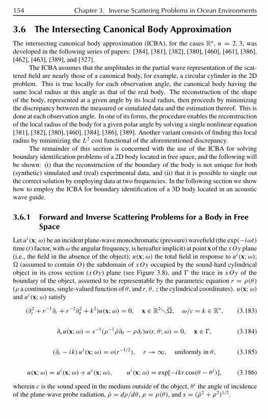
154 Chapter 3. Inverse Scattering Problems in Ocean Environments
3.6 The Intersecting Canonical Body ApproximationThe intersecting canonical body approximation (ICBA), for the cases Rn, n = 2, 3, wasdeveloped in the following series of papers: [384], [381], [382], [380], [460], [461], [386],[462], [463], [389], and [327].
The ICBA assumes that the amplitudes in the partial wave representation of the scat-tered field are nearly those of a canonical body, for example, a circular cylinder in the 2Dproblem. This is true locally for each observation angle, the canonical body having thesame local radius at this angle as that of the real body. The reconstruction of the shapeof the body, represented at a given angle by its local radius, then proceeds by minimizingthe discrepancy between the measured or simulated data and the estimation thereof. This isdone at each observation angle. In one of its forms, the procedure enables the reconstructionof the local radius of the body for a given polar angle by solving a single nonlinear equation[381], [382], [380], [460], [384], [386], [389]. Another variant consists of finding this localradius by minimizing the L2 cost functional of the aforementioned discrepancy.
The remainder of this section is concerned with the use of the ICBA for solvingboundary identification problems of a 2D body located in free space, and the following willbe shown: (i) that the reconstruction of the boundary of the body is not unique for both(synthetic) simulated and (real) experimental data, and (ii) that it is possible to single outthe correct solution by employing data at two frequencies. In the following section we showhow to employ the ICBA for boundary identification of a 3D body located in an acousticwave guide.
3.6.1 Forward and Inverse Scattering Problems for a Body in FreeSpace
Let ui(x;ω) be an incident plane-wave monochromatic (pressure) wavefield (the exp(−iωt)time (t) factor, withω the angular frequency, is hereafter implicit) at point x of the xOy plane(i.e., the field in the absence of the object); u(x;ω) the total field in response to ui(x;ω); (assumed to contain O) the subdomain of xOy occupied by the sound-hard cylindricalobject in its cross section (xOy) plane (see Figure 3.8), and the trace in xOy of theboundary of the object, assumed to be representable by the parametric equation r = ρ(θ)
(ρ a continuous, single-valued function of θ , and r, θ, z the cylindrical coordinates). u(x;ω)and ui(x;ω) satisfy
(∂2r + r−1∂r + r−2∂2
θ + k2)u(x;ω) = 0, x ∈ R2, ω/c = k ∈ R∗, (3.183)
∂νu(x;ω) = s−1(ρ−1ρ∂θ − ρ∂r)u(r, θ;ω) = 0, x ∈ , (3.184)
(∂r − ik) us(x;ω) = o(r−1/2), r → ∞, uniformly in θ, (3.185)
u(x;ω) = ui(x;ω)+ us(x;ω), ui(x;ω) = exp[−ikr cos(θ − θ i)], (3.186)
wherein c is the sound speed in the medium outside of the object, θ i the angle of incidenceof the plane-wave probe radiation, ρ = dρ/dθ , ρ = ρ(θ), and s = (ρ2 + ρ2)1/2.

3.6. The Intersecting Canonical Body Approximation 155
Figure 3.8. Scattering configuration.
The forward scattering (measurement) problem is: Givenω, c, ui(x;ω), and, deter-mineu(x;ω) at all points on the circumscribing circleb of radiusb > ρ = Maxθ∈[0,2π [ ρ(θ).
Of particular interest here is the inverse scattering problem: Given ω, c, ui(x, ω), b,and the simulated or measured field on b, determine the location, size, and shape of theobject embodied by the so-called shape function ρ(θ), knowing a priori that (i) the originO is somewhere within the object, and (ii)
b > ρ(θ) > ρ0, ρ0 > 0, b > 0, (3.187)
wherein ρ0 is assumed to be a known positive real constant (as is b). Note that in the inverseproblem, u(x;ω) is unknown everywhere except on b.
156 Chapter 3. Inverse Scattering Problems in Ocean Environments
3.6.2 A Method for the Reconstruction of the Shape of the BodyUsing the ICBA as the Estimator
The estimator appeals to the ICBA [461], [381], [382], [460], [380], the mathematicalexpression of which is
u(x;ω)− ui(x;ω) = uICBA(x;ω)− ui(x;ω)
≡N∑
n=−Nan(τ (θ), θ)H
(1)n (kr)e
inθ , r ≥ τ(θ), θ ∈ [0, 2π [,(3.188)
wherein N = O(kρ),
an(τ (θ), θ) = − Jn(kτ (θ)
H(1)n (kτ (θ)
e−in(θi+π/2) ∀n ∈ −N, . . . ,−1, 0, 1, . . . , N, (3.189)
H(1)n ( . ) is the nth-order Hankel function of the first kind, Jn( . ) the nth-order Bessel
function, Zn(ζ ) = dZn(ζ )/dζ , and τ(θ) is the trial boundary shape function (which, ifthe inverse problem is solved exactly, is identical to ρ(θ)). The ICBA furnishes the exactsolution for scattering from a sound-hard circular cylinder of radius a and center O (i.e.,the case τ = a) provided N → ∞. It also furnishes an approximate solution to theforward-scattering problem for cylindrical obstacles of more general shape [461].
Let ui , us , u designate synthetic (simulated) or real (experimental) data pertainingto the incident, scattered, and total field, respectively, for the (real) body whose (real) shape(defined by the function ρ(θ)) is unknown and to be determined. Let ui , us , u designatethe estimated incident, scattered, and total field for a trial body with trial shape τ(θ). Toreconstruct the entire shape of the body requires finding ρ(θ) for all values of θ . In principle,we can identify the reconstructed value of ρ(θ) with that τ(θ) for which a discrepancyfunctional between the measured and estimated fields vanishes. Practically speaking, thisis done atM measurement angles θm;m = 1, 2, . . . ,M, so that the discretized version of, embodied in the set τ(θm);m = 1, 2, . . . ,M, is recovered from the set ofM equations(i.e., the discretized form of the discrepancy functional):
KICBA(τ(θm), θm;ω) ≡ u(b, θm;ω)− uICBA(b, θm;ω)
= u(b, θm;ω)− ui(b, θm;ω)−N∑
n=−Nan(τ (θm), θm)H
(1)n (kb)e
inθm
= 0, m = 1, 2, . . . ,M, (3.190)
wherein it is observed, with the help of (3.188)–(3.189), that themth equation depends onlyon the mth trial boundary shape parameter τ(θm). Although these equations are uncoupledin terms of τ(θm); m = 1, 2, . . . ,M, each one is nonlinear because each member of theset an(τ (θm), θm) is a nonlinear function of τ(θm).
3.6. The Intersecting Canonical Body Approximation 157
3.6.3 Use of the K Discrepancy Functional and a PerturbationTechnique
We assume that
kτ(θ) = kd + kεf (θ), kρ(θ) = ka + kεg(θ), (3.191)
where a, d , and ε are positive real constants, f (θ) has the same functional properties asτ(θ), g(θ) has the same functional properties as ρ(θ), |f (θ)| ≤ 1, |g(θ)| ≤ 1, and
kε 1. (3.192)
To zeroth order in kε, us(b, θm;ω) is just the field scattered by a circular cylinder of radiusa and center atO, which, if it were simulated or measured in an exact manner, would be ofthe form
us(b, θm;ω) = −∞∑
n=−∞
Jn(ka)
H(1)n (ka)
e−in(θi+π/2)H (1)
n (kb)einθm, (3.193)
whereas the ICBA representation of the estimated scattered field takes the same form, withd replacing a.
At this stage, rather than attempt to solve the system (3.190), we prefer to return to itscontinuous form, which we project onto the set of Fourier basis functions exp(−imθ) ∀m ∈Z. The inverse problem thus reduces to the recovery of d from the following set ofequations:
Km :=∫ 2π
0KICBA(τ(θ), θ, ω) exp(−imθ)dθ = 0 ∀m ∈ Z, (3.194)
which, after use of the identity∫ 2π
0ei(n−m)θdθ = 2πδmn ∀m, n ∈ Z (3.195)
(with δmn the Kronecker symbol), yields
Km =[− Jm(ka)
H(1)m (ka)
+ Jm(kd)
H(1)m (kd)
]H(1)m (kb)e
−im(θi+π/2) = 0 ∀m ∈ Z, (3.196)
from which we deduce, after using the relation [313] H(1)n (ζ ) = Jn(ζ ) + iYn(ζ ) between
the Hankel (H ), Bessel (J ), and Neumann (Y ) functions,
−Jm(ka)Ym(kd)+ Jm(kd)Ym(ka) = 0 ∀m ∈ Z. (3.197)
A consequence of this expression, from which we now try to determine d, is that if d isa solution of (3.197) for a finite subset of Z, then it must be a solution of (3.197) for theremainder of values of m in Z.

158 Chapter 3. Inverse Scattering Problems in Ocean Environments
An obvious solution of (3.197) is d = a, which is the correct solution to order (kε)0
for the shape function, since τ(θ) = d and ρ(θ) = a to zeroth order in kε, but this does notnecessarily mean that it is the only solution.
Consider the subset of equations (3.197) for which |m| kd and assume also thatka is such that |m| ka. We use the general formula [313]
−Zm(ζ ) = −Zm+1(ζ )+ m
ζZm(ζ ) (3.198)
and the following asymptotic forms of the Bessel and Neumann functions [313]:
Jm(ζ ) ∼√
2
πζcos
(ζ − πm
2− π
4
),
Ym(ζ ) ∼√
2
πζsin
(ζ − πm
2− π
4
), |m| ζ,
(3.199)
to find
Jm(ζ ) ∼ −√
2
πζsin
(ζ − πm
2− π
4
),
Ym(ζ ) ∼√
2
πζcos
(ζ − πm
2− π
4
), |m| ζ,
(3.200)
which enable us to obtain the asymptotic form of (3.197), from which it ensues that
sin(kd − ka) ∼ 0 ∀|m| kd, ka, (3.201)
the solutions of which are
d = a + lπ
kl ∈ Z ∀|m| kd, ka. (3.202)
A similar type of asymptotic analysis shows that (3.202) possesses only the single solutiond = a in the regime |m| ' kd , |m| ' ka.
Equation (3.202) indicates the possible existence of more than one solution of theinverse problem.
3.6.4 More on the Ambiguity of Solutions of the Inverse ProblemArising from Use of the ICBA
Instead of actually solving (i.e., looking for the roots of) each member of the set in (3.197), wecan rather search for the set of shape parameters τ(θm); m = 1, 2, . . . ,M by minimizingthe cost functionals
J (τ(θm, θm;ω)) =∣∣∣∣∣us(b, θm;ω)−
L∑n=−L
an(τ (θm), θm)H(1)n (kb)e
inθm
∣∣∣∣∣2
, m = 1, 2, . . . ,M,
(3.203)
3.6. The Intersecting Canonical Body Approximation 159
and again apply the perturbation method to zeroth order in kε so as to find, on account ofthe results of the preceding section,
J
(a + lπ
k, θm;ω
)
≈∣∣∣∣∣∣∑
|n|≈kd,ka
[−Jn(ka)Yn(ka + lπ)+ Jn(ka + lπ)Yn(ka)] ein(θ−θ i−π/2)
∣∣∣∣∣∣2
(3.204)
(wherein is finite for l = 0), whence J (a, θ;ω) = 0 ∀θ ∈ [0, 2π [, which indicatesthat the zeroth-order perturbation J cost functional possesses a global minimum when d isat its correct value d = a (this being true for all angles). This is a reassuring result, butdoes not mean that there do not exist local minima for other values of d. In fact, as shownempirically in [327], [330], [328], J (a + lπ/k, θ;ω) does not vanish for values of l otherthan 0, but indeed exhibits a series of local minima at positions not far removed from thosepredicted by (3.202).
3.6.5 Method for Reducing the Ambiguity of the BoundaryReconstruction
The principal result of the preceding sections is the zeroth-order perturbation prediction
d = a + lπ
k, l ∈ L, (3.205)
wherein L is the finite subset of Z for which d is within the bounds of ρ written in (3.187).We hypothesize (admittedly encouraged by the results of numerical experiments [327]) thatif the perturbation analysis were carried out to higher order it would give a relation of thesort
τ(θ) ≈ ρ(θ)+ lπ
k, l ∈ L. (3.206)
This relation signifies that the inversion process should lead to a series of nearly homotheticreconstructed bodies, one of which (i.e., the one for which l = 0) is nearly the real body.Thus, we are faced with the problem of eliminating or at least reducing the nonuniquenessexpressed by (3.206).
Let us term the curves for which l = 0 “artifacts.’’ Equation (3.206) tells us that thecurves relative to the artifacts, contrary to the one relative to the boundary of the real body,depend on the wavenumber of the probe radiation. This suggests that the boundary we arelooking for is the only one that does not change when the frequency of the probe radiation ischanged. It is then a relatively simple matter to devise a scheme that filters out the artifactsfrom two sets of data obtained at two frequencies [327].
This scheme has the following ingredients [327]. First, divide the interval [0, 2π [ intoS sectors, which amounts to discretizing θ according to θs = (s − 1)δs , s = 1, 2, . . . , S,where δs = 2π/S. Second, divide the interval [ρ0, b] into I subintervals Ii , which amounts
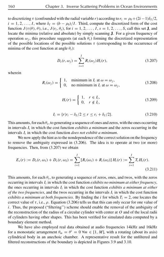
160 Chapter 3. Inverse Scattering Problems in Ocean Environments
to discretizing τ (confounded with the radial variable r) according to ri = ρ0+(2i−1)δI /2,i = 1, 2, . . . , I , where δI = (b − ρ0)/I . Third, compute the discretized form of the costfunction J (τ(θ), θ), i.e., J (ri, θs), for i = 1, 2, . . . , I , s = 1, 2, . . . , S, call this set J, andlocate the minima (relative and absolute) by simply scanning J. For a given frequency ofoperation ωj , this procedure suggests (at each θs) forming the discretized representationof the possible locations of the possible solutions τ (corresponding to the occurrence ofminima of the cost function at angle θs):
Ds(r, ωj ) =I∑i=1
Ri(ωj )Hi(r), (3.207)
wherein
Ri(ωj ) =
1, minimum in Ii at ω = ωj ,
0, no minimum in Ii at ω = ωj ,(3.208)
Hi(r) =
1, r ∈ Ii,0, r /∈ Ii, (3.209)
Ii = r|ri − δI /2 ≤ r ≤ ri + δI /2. (3.210)
This amounts, for each θs , to generating a sequence of ones and zeros, with the ones occurringin intervals Ii in which the cost function exhibits a minimum and the zeros occurring in theintervals Ii in which the cost function does not exhibit a minimum.
We now apply the hint as to the nondependence of the correct solution on the frequencyto remove the ambiguity expressed in (3.206). The idea is to operate at two (or more)frequencies. Then, from (3.207) we obtain
Es(r) := Ds(r, ω1)+Ds(r, ω2) =I∑i=1
[Ri(ω1)+ Ri(ω2)]Hi(r) :=I∑i=1
TiHi(r).
(3.211)
This amounts, for each θs , to generating a sequence of zeros, ones, and twos, with the zerosoccurring in intervals Ii in which the cost function exhibits no minimum at either frequency,the ones occurring in intervals Ii in which the cost function exhibits a minimum at eitherof the two frequencies, and the twos occurring in the intervals Ii in which the cost functionexhibits a minimum at both frequencies. By finding the i for which Ti = 2, one locates thecorrect value of τ , i.e., ρ. Equation (3.206) tells us that this can only occur for one value ofi. Thus, the proposed (“filtering’’) scheme should enable the removal of the ambiguity ofthe reconstruction of the radius of a circular cylinder with center at O and of the local radiiof cylinders having other shapes. This has been verified for simulated data computed by aboundary element method.
We have also employed real data obtained at audio frequencies 14kHz and 16kHzfor a monostatic arrangement θm = θ i = 0 ∀m ∈ [1,M], with a rotating (about its axis)cylindrical body in an anechoic chamber. A representative result for the unfiltered andfiltered reconstructions of the boundary is depicted in Figures 3.9 and 3.10.

3.6. The Intersecting Canonical Body Approximation 161
Figure 3.9. Real data case. Polar plot of the minima of the cost functionals J atthe two frequencies 14kHz (+) and 16kHz (∗) for an acoustically hard hexagonal cylin-der [328].
Figure 3.10. Filtered reconstruction (squares) of the shape function of the hex-agonal cylinder (continuous curve). The real data at the two frequencies 14kHz and 16kHzwere employed in the filtering scheme for this task. The reconstruction (not shown) is lessambiguous with synthetic data [328].

162 Chapter 3. Inverse Scattering Problems in Ocean Environments
Figure 3.11. Obstacle in an acoustic wave guide (shallow sea) configuration.
3.7 The ICBA for Shallow Oceans: Objects of Revolution
Let the ocean occupy the region := R2 × [0, h], the surface being designated by 0 :=R2 × 0, and the bottom by h := R2 × h.9
ICBA takes advantage of the fact that whatever the shape of the scatterer, for anycylinder Dd having axis perpendicular to the wave guide surfaces and enclosing the body(see Figure 3.11), the total wave field may be represented in −Dd by
u(r, θ, z) = uinc(r, θ, z) (3.212)
+∞∑n=1
∞∑m=0
φn(z)H(1)m (kanr)[Anm cos(mθ)+ Bnm sin(mθ)],
where the incident “plane wave’’ is
uinc(r, θ, z) =N∑n=1
∞∑m=0
imεmφn(z)φn(z0)Jm(kanr) cosm(θ − θ0) (3.213)
and
N =⌊
1
2+ kh
π
⌋,
φn(z) =√
2
hsin
((2n− 1)πz
2h
),
an =√
1 − (n− 12 )
2π2
k2h2.
9The authors also have written a series of papers using ICBA to image objects in a shallow ocean; in this regardsee [66], [67], [68], [69], [70], [71], [73], [74].
3.7. The ICBA for Shallow Oceans: Objects of Revolution 163
Here the φn(z) are modal solutions, εm = 1 form = 0, and εm = 2 form > 0. The functionsJm and H(1)
m are the mth-order Bessel and Hankel functions of the first kind, respectively.For the case in which the object is a sound-soft circular cylinder coaxial with the
z-axis and having radius R, the coefficients Anm and Bnm are given by [208], [207]
Anm =
−εmimφn(z0) cos(mθ0)Jm(kanR)
H(1)m (kanR)
for 1 ≤ n ≤ N,0 for n > N,
Bnm =
−εmimφn(z0) sin(mθ0)Jm(kanR)
H(1)m (kanR)
for 1 ≤ n ≤ N,0 for n > N.
Thus the total pressure field may be represented by [208], [207],
u(r, θ, z) = ui(r, θ, z)+N∑n=1
∞∑m=0
Cnm(a) cos(m[θ − θ0])φn(z)H (1)m (kanr), (3.214)
where
Cnm(R) = −εmimφn(z0)Jm(kanR)
H(1)m (kanR)
.
This permits the generalization of the method of Scotti and Wirgin [381], [382] for objectsin R3 to the case of objects in a wave guide, which can be parameterized by r = ρ(θ, z),0 ≤ θ ≤ 2π , 0 ≤ z ≤ h.
Gilbert et al. [208], [207] posed the following inverse problem: Determine the dis-cretized shape functionρqp = ρ(θq, zp)on the index setq ∈ 1, . . . ,Q andp ∈ 1, . . . , P such that
u∗(rb, θq, zp)− [ui(rb, θq, zp)
+N∑n=1
M∑m=0
Cnm(ρqp) cos(m[θq − θ0])φn(zp)H (1)
m (kanrb)] ∼= 0,
whereu∗(rb, θq, zp) are the given data for the total field on a cylinder of radius rb. Numericalsimulations using the above method led to very good results [208], [207]. However, as thesame procedure was used to invert the data as to generate it, this could be considered ascommitting the “inverse crime,’’ even though different lengths of expansions were used forthe forward and inverse computations.
3.7.1 Derivation of the Recurrences for Calculation of theScattered Field
The method of variation of boundaries [58, 59, 60, 61] is applicable to the situation wherethe scattering object is a small perturbation of a shape for which the scattering problemis explicitly solvable. In the case of an ocean of uniform depth the appropriate canonicalshape is the circular cylinder for which the solution to the scattering problem was stated in
164 Chapter 3. Inverse Scattering Problems in Ocean Environments
the previous section. In [72] we used this method to generate the acoustic field for depthindependent cylinders having a cross section of the form r = R + δf (θ). In this sectionwe consider solids of revolution of the form r = R + δf (z). In the method of variation ofboundaries the scattered wave is expanded in terms of the parameter δ as
usc(r, θ, z) =∞∑l=0
δlul(r, θ, z) (3.215)
where each ul is assumed to have the form of the canonical solution
ul(r, θ, z) =N∑n=1
∞∑m=0
φn(z)H(1)m (kanr)
(cnm;l cosmθ + dnm;l sinmθ
).
The unknown coefficients cnm;l and dnm;l are determined by the condition imposed at thesurface of the scatterer.
At the surface r = R + δf (z) of the obstacle, assuming a sound-soft boundarycondition,
uinc(R + δf (z), θ, z) = −∞∑p=0
δpup(R + δf (z), θ, z). (3.216)
By setting δ = 0 we obtain from
N∑n=1
∞∑m=0
imεmφn(z)φn(z0)Jm(kanR) (cosmθ0 cosmθ + sinmθ0 sinmθ)
= −N∑n=1
∞∑m=0
φn(z)H(1)m (kanR)
(cnm;0 cosmθ + dnm;0 sinmθ
)the first expansion coefficients
cnm;0 = − 1
H(1)m (kanR)
imεmφn(z0)Jm(kanR) cosmθ0,
dnm;0 = − 1
H(1)m (kanR)
imεmφn(z0)Jm(kanR) sinmθ0.
The higher order coefficients are obtained by differentiating (3.222) l times to get
dl
dδluinc = −
∞∑p=0
l∑q=0
(l
q
)dq
dδqδpdl−q
dδl−qup.
Upon setting δ = 0 we get
dl
dδluinc
∣∣∣∣δ=0
= −l∑
p=0
(l
p
)p! d
l−p
dδl−pup
∣∣∣∣δ=0
= −l!l∑
p=0
1
(l − p)!dl−p
dδl−pup
∣∣∣∣δ=0
,
3.7. The ICBA for Shallow Oceans: Objects of Revolution 165
whence
ul|δ=0 = − 1
l!dl
dδluinc
∣∣∣∣δ=0
−l−1∑p=0
1
(l − p)!dl−p
dδl−pup
∣∣∣∣δ=0
. (3.217)
One may then extract the coefficients cjm;l and djm;l after rather long analytic calculationsto be given in terms of the recurrence relations [72]
cjm;l = −1
Hjm;0
(imεm cosmθ0
N∑n=1
φn(z0)Jnm;l
·( n∑q=1
q;l1√hεn−q
Ij,n−q +N∑
q=n+1
q;l1√hεq−n
Ij,q−n −N∑q=1
q;l1√
hεq+n−1Ij,q+n−1
)
+N∑n=1
l−1∑p=0
Hnm;l−p( n∑q=1
q;l−p1√hεn−q
Ij,n−q +N∑
q=n+1
q;l−p1√hεq−n
Ij,q−n
−N∑q=1
q;l−p1√
hεq+n−1Ij,q+n−1
)cnm;p
)
djm;l = −1
Hjm;0
(imεm sinmθ0
N∑n=1
φn(z0)Jnm;l
·( n∑q=1
q;l1√hεn−q
Ij,n−q +∞∑
q=n+1
q;l1√hεq−n
Ij,q−n −∞∑q=1
q;l1√
hεq+n−1Ij,q+n−1
)
+N∑n=1
l−1∑p=0
Hnm;l−p( n∑q=1
q;l−p1√hεn−q
Ij,n−q +∞∑
q=n+1
q;l−p1√hεq−n
Ij,q−n
−∞∑q=1
q;l−p1√
hεq+n−1Ij,q+n−1
)dnm;p
).
Here the q;l are the Fourier coefficients of f (z)l with respect to the modal solutionsφq(z), namely,
f (z)l =∞∑q=1
q;lφq(z).
To complete the recursion formulas we need to determine these coefficients. In [72], recur-sive relations for the coefficients of the Fourier series of
f (z)l =∞∑q=1
q;lφq(z)
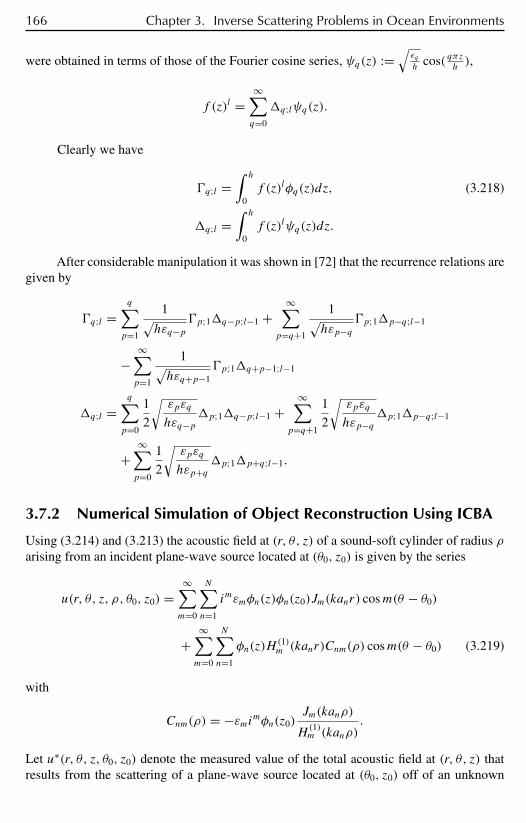
166 Chapter 3. Inverse Scattering Problems in Ocean Environments
were obtained in terms of those of the Fourier cosine series, ψq(z) :=√εqh
cos( qπzh),
f (z)l =∞∑q=0
q;lψq(z).
Clearly we have
q;l =∫ h
0f (z)lφq(z)dz, (3.218)
q;l =∫ h
0f (z)lψq(z)dz.
After considerable manipulation it was shown in [72] that the recurrence relations aregiven by
q;l =q∑p=1
1√hεq−p
p;1q−p;l−1 +∞∑
p=q+1
1√hεp−q
p;1p−q;l−1
−∞∑p=1
1√hεq+p−1
p;1q+p−1;l−1
q;l =q∑p=0
1
2
√εpεq
hεq−pp;1q−p;l−1 +
∞∑p=q+1
1
2
√εpεq
hεp−qp;1p−q;l−1
+∞∑p=0
1
2
√εpεq
hεp+qp;1p+q;l−1.
3.7.2 Numerical Simulation of Object Reconstruction Using ICBA
Using (3.214) and (3.213) the acoustic field at (r, θ, z) of a sound-soft cylinder of radius ρarising from an incident plane-wave source located at (θ0, z0) is given by the series
u(r, θ, z, ρ, θ0, z0) =∞∑m=0
N∑n=1
imεmφn(z)φn(z0)Jm(kanr) cosm(θ − θ0)
+∞∑m=0
N∑n=1
φn(z)H(1)m (kanr)Cnm(ρ) cosm(θ − θ0) (3.219)
with
Cnm(ρ) = −εmimφn(z0)Jm(kanρ)
H(1)m (kanρ)
.
Let u∗(r, θ, z, θ0, z0) denote the measured value of the total acoustic field at (r, θ, z) thatresults from the scattering of a plane-wave source located at (θ0, z0) off of an unknown

3.7. The ICBA for Shallow Oceans: Objects of Revolution 167
–2
–1
0
1
2
–2
–1
0
1
20
2
4
6
8
10
Figure 3.12. Two-level cylinder.
–2
–1
0
1
2
–2
–1
0
1
20
2
4
6
8
10
Figure 3.13. Indentedparabolic spindle.
object. For measured fields u∗(r, θ, z, θq0 , zp
0 ) arising from sources at positions (θq, zp),q = 1, . . . ,Q0, p = 1, . . . , P0, which are assumed to be distinguishable by the receiver,the ICBA method determines the radius ρ of the object at angle θ and depth z by minimizingthe objective function
fobj (ρ) =√√√√ P0∑p=1
Q0∑q=1
∣∣u∗(r, θ, z, θq0 , zp
0 )− u(r, θ, z, ρ, θq0 , zp0 )∣∣2.
We considered the case where a single source/receiver unit emits a monochromaticplane wave from a position (r, θ, z) and measures the resulting field u∗ at the same position.In this circumstance (θ0, z0) = (θ, z) and the objective function simplifies to
fobj (ρ) = ∣∣u∗(r, θ, z, θ, z)− u(r, θ, z, ρ, θ, z)∣∣ . (3.220)
To test the ICBA method, measured data was simulated for wavenumbers k = 4, 8and 12 for the following two shapes for the scatterer.
(1) A two-level cylinder (Figure 3.12):
g(z) =
1, a ≤ z ≤ b,12 otherwise,
with a = 3 and b = 6.(2) An indented parabolic spindle (Figure 3.13):
g(z) = 4
( 12 h+1)2
z( 12h+ 1 − z), 0 ≤ z ≤ 1
2h,
4( 1
2 h+1)2(z+ 1 − 1
2h)(h− z), 12h < z ≤ h.
The ICBA method seeks to find the global minimum ρ of the objective function(3.220) at a specified direction and depth (θ, z). The objective function may have multiplelocal minima. Figures 3.14 and 3.15 show 3D reconstructions of the two test objects forwavenumber k = 12.
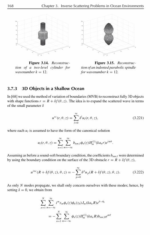
168 Chapter 3. Inverse Scattering Problems in Ocean Environments
–2
–1
0
1
2
–2
–1
0
1
20
2
4
6
8
10
Figure 3.14. Reconstruc-tion of a two-level cylinder forwavenumber k = 12.
–2
–1
0
1
2
–2
–1
0
1
20
2
4
6
8
10
Figure 3.15. Reconstruc-tion of an indented parabolic spindlefor wavenumber k = 12.
3.7.3 3D Objects in a Shallow Ocean
In [68] we used the method of variation of boundaries (MVB) to reconstruct fully 3D objectswith shape functions r = R + δf (θ, z). The idea is to expand the scattered wave in termsof the small parameter δ
usc(r, θ, z) =∞∑l=0
δlul(r, θ, z), (3.221)
where each ul is assumed to have the form of the canonical solution
ul(r, θ, z) =∞∑n=1
∞∑m=−∞
bnm;lφn(z)H (1)m (kanr)e
imθ .
Assuming as before a sound-soft boundary condition, the coefficients bnm;l were determinedby using the boundary condition on the surface of the 3D obstacle r = R + δf (θ, z),
uinc(R + δf (θ, z), θ, z) = −∞∑p=0
δpup(R + δf (θ, z), θ, z). (3.222)
As only N modes propagate, we shall only concern ourselves with these modes; hence, bysetting δ = 0, we obtain from
N∑n=1
∞∑m=−∞
imεmφn(z)φn(z0)Jm(kanR)eθ−θ0
= −N∑n=1
∞∑m=−∞
φn(z)H(1)m (kanR)bnm;0emθ
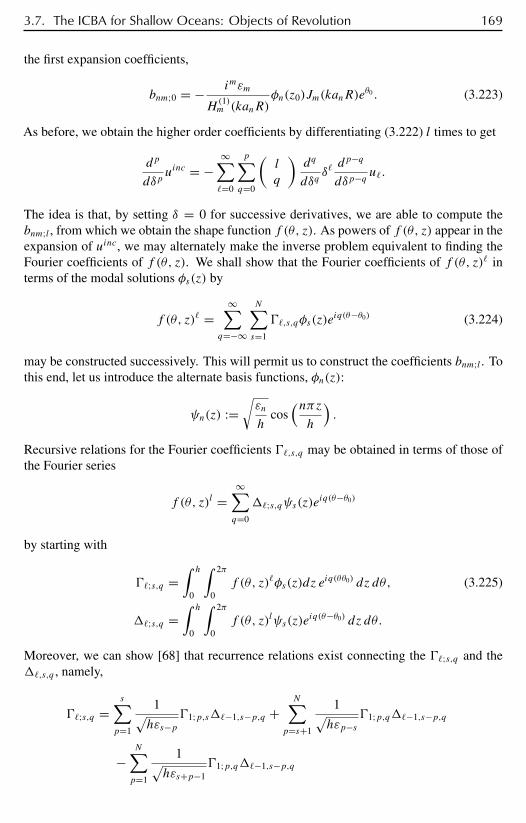
3.7. The ICBA for Shallow Oceans: Objects of Revolution 169
the first expansion coefficients,
bnm;0 = − imεm
H(1)m (kanR)
φn(z0)Jm(kanR)eθ0 . (3.223)
As before, we obtain the higher order coefficients by differentiating (3.222) l times to get
dp
dδpuinc = −
∞∑=0
p∑q=0
(l
q
)dq
dδqδdp−q
dδp−qu.
The idea is that, by setting δ = 0 for successive derivatives, we are able to compute thebnm;l , from which we obtain the shape function f (θ, z). As powers of f (θ, z) appear in theexpansion of uinc, we may alternately make the inverse problem equivalent to finding theFourier coefficients of f (θ, z). We shall show that the Fourier coefficients of f (θ, z) interms of the modal solutions φs(z) by
f (θ, z) =∞∑
q=−∞
N∑s=1
,s,qφs(z)eiq(θ−θ0) (3.224)
may be constructed successively. This will permit us to construct the coefficients bnm;l . Tothis end, let us introduce the alternate basis functions, φn(z):
ψn(z) :=√εn
hcos
(nπzh
).
Recursive relations for the Fourier coefficients ,s,q may be obtained in terms of those ofthe Fourier series
f (θ, z)l =∞∑q=0
;s,qψs(z)eiq(θ−θ0)
by starting with
;s,q =∫ h
0
∫ 2π
0f (θ, z)φs(z)dz e
iq(θθ0) dz dθ, (3.225)
;s,q =∫ h
0
∫ 2π
0f (θ, z)lψs(z)e
iq(θ−θ0) dz dθ.
Moreover, we can show [68] that recurrence relations exist connecting the ;s,q and the,s,q , namely,
;s,q =s∑p=1
1√hεs−p
1;p,s−1,s−p,q +N∑
p=s+1
1√hεp−s
1;p,q−1,s−p,q
−N∑p=1
1√hεs+p−1
1;p,q−1,s−p,q

170 Chapter 3. Inverse Scattering Problems in Ocean Environments
,s =s∑p=0
1
2
√εpεs
hεs−p1;p,q,p−s,q +
∞∑p=s+1
1
2
√εpεs
hεp−s1;p,q−1;p−s,q
+∞∑p=0
1
2
√εpεs
hεp+s1;p,q−1,p−s,q .
Following the same procedure as in the last subsection, Ou [332] has been able to reconstructcompletely 3D objects.

Chapter 4
Oceans over ElasticBasements
4.1 A Uniform Ocean over an Elastic SeabedIn the previous two chapters we have discussed wave propagation in acoustic wave guideswith a completely reflecting bottom and a pressure-release surface. In this section we willextend our discussion to the case of a time-harmonic point source in a water column with aninteractive elastic seabed. Our approach follows that given in our papers [185], [186], [203].
We assume a time-harmonic, point source is situated in a homogeneous, shallowocean of uniform depth h, which lies over an elastic seabed of finite depth b. Here the watercolumn occupies the region
f := (r, z) : 0 < r <∞, 0 < z < h
and the seabed occupies
s := (r, z) : 0 < r <∞, b < z < h.
The boundaries of these regions, shown in Figure 4.1, are given by f , s , and f s :
f := (r, z) : 0 < r <∞, z = 0,
f s := (r, z) : 0 < r <∞, z = h,
s := (r, z) : 0 < r <∞, z = b.
Imbedded in the water column is a hard, smooth scatterer, which occupies the regionD. Onthe ocean–seabed interface, both the reflection and transmission of acoustic energy occurs;namely, a portion of the energy leaves the ocean and enters the seabed. Another way ofdescribing this situation is to note that the total field consists of direct radiation, partialreflection off the sea floor, and scattered radiation off the object.
171

172 Chapter 4. Oceans over Elastic Basements
Figure 4.1
For convenience we write x := (x, y), the pressure field as p(x, z), and the verticaldisplacement as uzo(x, z). Similar notation will be used for future unknown variables. Werecall from Chapter 1 that these physical entities are related to each other by
p(x, z)+ k20p(x, z) = −δ(x − xs)δ(y − xs)δ(z− zs),
∂zp + ω2ρuzo = 0,
where ω is the frequency, ρw the density of ocean water, k0 = ω/c0 the wavenumber, and(xs, ys, zs) the source position.
As in the previous two chapters, it is assumed that the seabed is a homogeneous,isotropic medium. Moreover, we assume that the amplitude of the acoustic oscillations inthe seabed are sufficiently small to ensure the validity of a linear elasticity. In the seabed let$u := [ux, uy, uz] be the displacement vector and σij the components of the Cauchy stresstensor. The time-harmonic equations of motion are given by10
∂xσxx + ∂yσxy + ∂zσxz + ρsω2ux = 0, (4.1)
∂xσxy + ∂yσyy + ∂zσyz + ρsω2uy = 0, (4.2)
∂xσxz + ∂yσzy + ∂zσzz + ρsω2uz = 0. (4.3)
In the above assume we have isotropic constitutive relations, namely,
e = ∂xux + ∂yuy + ∂zuz, (4.4)10See Chapter 1.

4.1. A Uniform Ocean over an Elastic Seabed 173
σxx = λe + 2µ∂xux, (4.5)
σyy = λe + 2µ∂yuy, (4.6)
σzz = λe + 2µ∂zuz, (4.7)
σxy = µ(∂xuy + ∂yux), (4.8)
σxz = µ(∂xuz + ∂zux), (4.9)
σyz = µ(∂zuy + ∂yuz), (4.10)
whereλ,µ are Lamé coefficients andρs is the density of the seabed. The following boundaryand transmission conditions are used for the ocean–elastic-seabed model [53]:
p(x, 0) = 0, (4.11)
uzo(x, h−) = uz(x, h+), (4.12)
p(x, h−) = σzz = (x, h+) = (λe)(x, h+) (4.13)
+ 2(µ∂zuz)(x, h+) (4.14)
σxz = σyz = 0, (4.15)
whereas at bottom of the seabed, it is assumed that
uz(x, b) = 0, (4.16)
∂zσzz(x, b) = 0. (4.17)
By using the elasticity equations and (4.15)–(4.17), the problem can be reformulated asa seismology problem similar to the Lamb problem [221]. That is, one seeks the verticaldisplacement as a response to the normal-stress load on the shear-free interfacef s ; in otherwords, we seek the stress-to-displacement mapping
σzz(x, h+)→ uz(x, h
+).
In view of (4.14)–(4.15), this is equivalent to the vertical-displacement-to-normal-stressmap
T : T(p(x, h−)) = ∂zp(x, z)∣∣z=h− (4.18)
on the interface being linear. Therefore, how the water column and the seabed interact iscontained in the operator T, which provides a nonlocal condition.11 The reflecting seabedcan be treated as the special case when T ≡ 0. In this notation, scattering off a hard,submerged object is mathematically formulated by the system
p + k20p = −δ(x − xs)δ(y − ys)δ(z− zs), (x, z) ∈ c, (4.19)
p(x, 0) = 0, (4.20)
∂zp(x, z)∣∣z=h− = T (p(x, h)), (4.21)
11Kleinman and Angell (see [9]) have considered an impedance boundary condition, which corresponds to alocal condition. Then condition (1.19) reduces to ∂zp(x, z)
∣∣z=h− = T(p(x, h−)) ≡ ap(x, h−).

174 Chapter 4. Oceans over Elastic Basements
∂p
∂ν= 0. (4.22)
Here ν is taken to be the outward normal to ∂. In order to ensure that the waves areoutgoing, the separated solutions are represented in terms of Hankel functions of the firstkind and of order zero, H(1)
0 (√ξr).
4.1.1 The Boundary Integral Equation Method for the DirectProblem
Because the exterior problem inside a wave guide is an unbounded region with a finiteboundary, it is convenient to reformulate our problem as a boundary integral equation. Thispermits a reduction from a 3D unbounded region problem to a 2D, bounded region problem.The difficulty in applying the boundary element method depends on obtaining a suitablefundamental singularity for the entire ocean–seabed system. For example, a suitable singularsolution might be taken to be the Green’s function for the ocean–seabed system. We denotethis fundamental solution by G. G is the pressure field excited by a time-harmonic pointsource at (x0, y0, z0) in the object-free wave guide. G must then satisfy
G+ k20n(z)G = −δ(x − x0)δ(y − y0)δ(z− z0), (4.23)
G∣∣z=h = 0, (4.24)
∂zG∣∣z=h− = T (G
∣∣z=h−). (4.25)
We must show that this singular solution exists. We state this as a theorem but postpone theproof until later.
Theorem 4.1. The problem (4.23)–(4.25) has an axially symmetric solution for all ω ∈ R+except for a discrete, countable set of values ωj . Because of the axial symmetry of theequations about any point, the Green’s function may be expressed in the form G(|x −x0|, z, z0).
It shall be tacitly assumed in all subsequent discussions that the frequency ω is neverone of the exceptional ωj mentioned in the hypothesis. If G(|x − x0|, z, z0) is taken to bethe incident wave, the function defined as
p1(x, z) := p(x, z)−G(|x − xs |, z, zs)corresponds to the scattered wave. Clearly, p1(x, z) must satisfy
p1 + k20p1 = 0, (x, z) ∈ c, (4.26)
p1(x, h−) = 0, (4.27)
∂zp1(x, z)∣∣z=h− = T (p1(x, h−)), (4.28)
∂p1
∂ν
∣∣∂
= −∂G(|x − xs |, z, zs)∂ν
∣∣∂. (4.29)
Because of Huygens’s principle, each point on the object’s surface ∂ functions as a sourceof a scattered wave. This suggests that we represent p1 in terms of a single-layer potential,
4.1. A Uniform Ocean over an Elastic Seabed 175
namely as
p1(x, z) =∫∂
G(|x − xd |, z, zd)f (xd , zd)dSd, (4.30)
where f is an unknown density function that is to be determined. The following lemmamay be found in [185].
Lemma 4.2. The single-layer potential (4.30) satisfies equation (4.26), boundary condition(4.27), and transmission condition (4.28) for any f for which the integral exists.
Proof. For (xd , zd) ∈ , G(|x − xd |, z, zd) satisfies (4.23) and (4.24); hence, p1 satisfies(4.26) and (4.27). To show it also satisfies (4.28), the linearity of T may be used to compute
∂z
∫∂
G(|x − xd |, z, zd)f (xd , zd)dS ∣∣
z=0
=∫∂
∂zG(|x − xd |, z, zd)∣∣z=h−f (xd , zd)dSd
=∫∂
T(G(|x − xd |, z, zd)∣∣z=h−)f (xd , z0)dS
= T([∫
∂
G(|x − xd |, z, zd)f (xd , zd)dSd] ∣∣z=h−
).
To complete the verification that p1 may be expressed as a single-layer potential, it isnecessary to find an f such that the potential (4.30) satisfies (4.29).
Intuitively speaking, the propagating solution G(|x − x0|, z, z0) can be decomposedinto a direct-radiation term plus the combined effect of partial-reflection and transmission,namely if
γ (ρ, z, z0) := eik0√ρ2 + (z2 − z0)2
4π√ρ2 + (z− z0)2
,
then
G(|x − x0|, z, z0) = γ (|x − x1|, z, z0)+ G1(|x − x0|, z, z0). (4.31)
Since G1(|x − x0|, z, z0) as a function of the arguments z, x satisfies the homogeneousHelmholtz equation, it belongs to C1(1).
For any (x1, z1) ∈ ∂, the outward normal ν(x1,z1) exists. Take the directional deriva-tive ∂
∂ν(x1 ,z1)of the both sides of (4.30) and let (x, z) approach (x1, z1) along ν(x1,z1). Note
that the term ek0r1/4πr1 in (4.31) undergoes a jump discontinuity, whereas G1 does not.Therefore, it follows that
−1
2f (x1, z1)+
∫∂
∂G(|x1 − xd |, z1, zd)
∂ν(x1,z1)
f (xd , zd)dSd (4.32)
= −∂G(|x1 − xd |, z1, zd)
∂ν(x1,z1)
, (x1, z1) ∈ ∂,
176 Chapter 4. Oceans over Elastic Basements
or symbolically one may write this as the boundary integral equation
−1
2f (x, z)+ K∗
Gf (x, z) = g(x, z), (x, z) ∈ ∂,
where K∗G, the boundary integral operator associated with G, is defined by
f → K∗Gf (x, z) :=
∫∂
∂G(|x − xd |, z1, zd)
∂νx,zf (xd , zd)dSd.
This boundary integral equation is similar to the boundary integral equation for objectsimbedded inR3, modulo the extra term in its kernel. Because of the nature of this additionalterm the basic weak singularity of the kernel is preserved. More precisely, this may beformulated as the following lemma [185].
Lemma 4.3. If ∂ ∈ C2, then
K∗G : Hs−1/2(∂)
(compact)−→ Hs−1/2(∂).
Proof.K∗G = K∗
γ + K∗G1.
By a classical result [488], one has
K∗G : Hs−1/2(∂)
(compact)−→ Hs+1/2(∂).
For the second term, because G1 ∈ C1, it follows that
K∗G : Hs−1/2(∂)
(compact)−→ Hs−1/2(∂).
Therefore the lemma follows from the property of compactness.
The solvability and regularity of this integral equation may be investigated by standardmethods [107].
Theorem 4.4. If ∂ ∈ C2, the boundary integral equation is uniquely solvable inHs−1/2(∂)
if and only if the original problem has at most one solution Hs+1loc (
c).
Proof. Since K∗G is compact, the Fredholm alternative applies. Because of this it is necessary
only to consider the homogeneous equation
−1
2f + K∗
Gf = 0.
If this equation has a nontrivial solution f , then it is convenient to introduce the function
p2(x, z) :=∫∂
G(|x − xd |, z, zd)f (xd , zd)dSd,
4.1. A Uniform Ocean over an Elastic Seabed 177
which is just the single-layer potential with density f . By Lemma 4.2, we know that p2
satisfies (4.26)–(4.28), and by (4.29), it also satisfies the homogeneous boundary condition
∂p2
∂ν|∂ = 0.
Hence, p2 corresponds to a free oscillation that is identically zero if and only if the originalproblem has a unique solution. This completes the proof.
The boundary integral equation may then be solved for the density f and the acousticpressure field computed using the potential representation (4.30). Using a computationalpoint of view, the fact that the density f could be inHs−1/2, s > 0, allows us more freedomfor choosing boundary elements. Note that ∂G
∂νappears as the kernel and in the right-hand
side. Because both (x1, z1) and (xd , zd) run over ∂, while (xs , zs) is away from ∂, thenear-field approximation for the kernel is necessary; however, for the right-hand side it ispreferable to use the far-field approximation. With this purpose in mind, these two differentapproximations are constructed in the next section.
4.1.2 Far-Field and Near-Field Estimates for the Green’s Function
Denote the compressional wave and shear wave velocities in the seabed by cl and ct , and thecompressional wave velocity in the ocean as c0, which are related to the Lamé coefficientsand density by
c2o = λo
ρo, c2
l = λ+ 2µ
ρs, and c2
t = µ
ρs.
The corresponding wavenumbers are given by
ko = ω
co, kl = ω
cl, kt = ω
ct.
Because of axial symmetry it is convenient to introduce cylindrical coordinates, in whichthe equations for G and uzo become(
∂r + 1
r
)∂rG+ ∂2
zG+ k20G+ δ (r) δ (z− z0)
2πr= 0, (4.33)
ω2ρwuzo + ∂zG = 0, 0 < z < h.
We use the Helmholtz decomposition of the sediment displacement, using the potentials φand ψ , which satisfy the equations(
∂r + 1
r
)∂rφ + ∂2
z φ + k2l φ = 0, (4.34)
∂r
(∂r + 1
r
)ψ + ∂2
z ψ + k2t ψ = 0, h < z < b. (4.35)
In terms of these potentials, the displacements are given by
ur = ∂rφ − ∂zψ, (4.36)
178 Chapter 4. Oceans over Elastic Basements
uz =(∂r + 1
r
)ψ + ∂zφ, (4.37)
and the stresses are expressed as
σzz = λ
(∂zuz +
(∂r + 1
r
)ur
)+ 2µ∂zuz
= (λ+ 2µ)
(∂zuz +
(∂r + 1
r
)ur
)− 2µ
(∂r + 1
r
)ur
= −c2l ρsk
2l φ − 2µ
(∂r + 1
r
)ur
= −µk2t φ − 2µ
(∂r + 1
r
)ur, (4.38)
σzr = µ(∂ruz + ∂zur). (4.39)
In order to rewrite our expressions using the same order of Hankel transform, we introducethe symbol χ := (∂r + 1
r)ψ . By letting ∂r + 1
ract on (4.35), (4.36), and (4.39), we can
rewrite these as(∂r + 1
r
)∂rχ + ∂2
z χ + k2t χ = 0,(
∂r + 1
r
)ur =
(∂r + 1
r
)∂rφ − ∂zχ,
uz = ∂zφ + χ,σzz = µ
(−2
(∂r + 1
r
)∂rφ + 2∂zχ − k2
t φ
),
1
µ
(∂r + 1
r
)σzr =
(∂r + 1
r
)∂ruz + ∂z
(∂r + 1
r
)∂rφ − ∂2
z χ
=(∂r + 1
r
)∂ruz +
(∂r + 1
r
)∂r (∂zφ + χ)+ k2
t χ
= 2
(∂r + 1
r
)∂r(∂zφ + χ)+ k2
t χ .
In cylindrical coordinates the transmission conditions in terms of the displacement poten-tials are
∂zφ(b)+ χ(b) = 0, (4.40)(k2t + 2
(∂r + 1
r
)∂r
)∂zφ(b) (4.41)
+ 2
(∂r + 1
r
)∂rχ(b)+ 2k2
t χ(b) = 0. (4.42)
Inserting one of these into the other implies
∂zφ(b) = χ(b) = 0.
4.1. A Uniform Ocean over an Elastic Seabed 179
The Hankel transform of the function f is defined to be
f := H0(f ) =∫ ∞
0f (r)rJ0(kr)dr.
As k ∈ (0,∞), for convenience, we make the substitution k = √ξ .We now transform the
partial differential equations and the associated boundary transition conditions, using theidentity H0((∂r + 1
r)∂rF ) = −ξF , to obtain system
G∣∣z=0 = 0, (4.43)
∂2z G+ (k2
0 − ξ)G+ 1
2πδ(z− z0) = 0, (4.44)
∂2z φ + (k2
l − ξ)φ = 0, (4.45)
∂2z χ + (k2
t − ξ)χ = 0, (4.46)(ω2ρw(∂zφ + χ)+ ∂zG
) ∣∣z=h = 0, (4.47)(
G− µ((2ξ − k2t )φ + 2∂zχ)
) ∣∣z=h = 0, (4.48)(
−2ξ∂zφ + (k2t − 2ξ)χ
) ∣∣z=h = 0, (4.49)
χ∣∣z=b = ∂zφ
∣∣z=b = 0. (4.50)
These equations may be solved to obtain
G = 1
2π
C1
sinh
(√ξ − k2
0z
)√ξ − k2
0
−H(z− z0)
sinh
(√ξ − k2
0(z− z0)
)√ξ − k2
0
,φ = C2 cosh
(√ξ − k2
0(b − z)),
χ = C3
sinh
(√ξ − k2
0(b − z))
√ξ − k2
0
,
where H(z) is the Heaviside function. Substituting these into the transmission conditionsresults in a solution to the transformed ocean–seabed system [185]
G(ξ, z, z0) = 1
2π
L(ξ, h− z0)
L(ξ, h)
sinh
(√ξ − k2
0z
)√ξ − k2
0
−H(z− z0)
sinh
(√ξ − k2
0(z− z0)
)√ξ − k2
0
,
φ = 2ξ − k2t
2πµL(ξ, h)
sinh(√ξ − k2
t (b − h))
√ξ − kt2
sinh
(√ξ − k2
0z0
)√ξ − k2
0
cosh
(√ξ − k2
0(b − z)),

180 Chapter 4. Oceans over Elastic Basements
χ = 2ξ(ξ − k2l )
2πµL(ξ, h)
sinh
(√ξ − k2
l (b − h))
√ξ − k2
l
sinh
(√ξ − k2
0z0
)√ξ − k2
0
sinh
(√ξ − k2
0(b − z))
√ξ − k2
0
.
Here the function L(ξ, z) is defined to be
L(ξ, z) := A cosh
(√ξ − k2
0z
)+ B
sinh
(√ξ − k2
0z
)√ξ − k2
0
(4.51)
with
A(ξ) := (k2t − 2ξ)2 cosh
(√ξ − k2
l (b − h)) sinh
(√ξ − k2
t (b − h))
√ξ − k2
t
,
− 4ξ(ξ − k2l )
sinh
(√ξ − k2
l (b − h))
√ξ − k2
l
cosh
(√ξ − k2
t (b − h)),
B(ξ) := βk4t (ξ − k2
l )
sinh
(√ξ − k2
l (b − h))
√ξ − k2
l
sinh(√ξ − k2
t (b − h))
√ξ − k2
t
.
Recall that the solution may be represented using the Hankel inversion theorem as
G(r, z, z0) =∫ ∞
0kG(ξ, z, z0)J0(kr)dk = 1
2
∫ ∞
0G(ξ, z, z0)J0(
√ξr)dξ.
Since this integral may not be obtained in closed form, we approximate it. It is interesting thattwo different procedures for approximating G lead, respectively, to a far-field approximationand a near-field approximation, depending on the particular inversion method used.
4.1.3 The Far-Field Approximation
To get a far-field representation, we first continue G(·, z, z0) to the complex ξ -plane. For = | |eθi , −π < θ ≤ π , we choose the branch
√ = √| |eθi/2. Note that both
cosh√ z and sinh
√ z/
√ are continuous across the branch cut. Hence, as A, B, and
L(·, z) are entire functions of ξ , we conclude that G is a meromorphic function. From theexpression for L(ξ, z), one has
L(ξ, h− z0)
L(ξ, h)∼
cos
(√ξ − k2
0(h− z0)
)cosh
(√ξ − k2
0h
) as |ξ | → ∞, |Imξ | > ε > 0,

4.1. A Uniform Ocean over an Elastic Seabed 181
which implies, excluding neighborhoods of the poles, that G(ξ, z, z0) is bounded in theentire ξ -plane.
Whether G(ξ, z, z0) is Hankel invertible or not depends on the location of the zerosof L(·, h). Let ξj ∞j=0 be the simple zeros of L(·, h) and ξ ∗
j Nj=0 be the multiple zeros
(note that from the asymptotic behavior of L(·, h), the number of multiple zeros of L(·, h)is finite). By using the Mittag-Leffler decomposition, one obtains
G(ξ, z, z0) =∞∑j=0
Resξj G1
ξ − ξj +N∑j=0
cj (z)
(ξ − ξ ∗j )dj
= 1
2π
∞∑j=0
L(ξj , h− z0)
∂ξ L(ξj , h)
sinh
(√ξj − k2
0z
)√ξj − k2
0
1
ξ − ξj +N∑j=0
cj (z)
(ξ − ξ ∗j )dj.
From the asymptotic behavior of L(·, h), it follows that the series converges. The three casesbelow, which are interesting, follow from a simple calculation using the inverse transform.
• For negative or complex ξj or ξ ∗j , the Hankel inversion of the term 1/(ξ − ξj ) or
1/(ξ − ξ ∗j ) exits in the normal sense; in particular, for negative ξj we have
H−10
(1
ξ − ξj)
=∫ ∞
0
kJ0(kr)
k2 − ξj dk = 1
2
∫ ∞
0
J0(√ξj r)
ξ − ξj dξ = K0
(√−ξ−
j r).
The inversion of 1/(ξ − ξ ∗j )dj can obtained by differentiating the above dj − 1 times
with respect to ξj and expressed in terms of the Kn, n = 0, 1, . . . , dj − 1. Since theKn(x) decrease exponentially, these negative zeros don’t actually make a significantcontribution to the far field.
• For positive zero ξj , the Hankel inversion of 1/(ξ−ξj ) exists in the Cauchy principle-value (p.v.) sense and
H(1)0 (
√ξj r) = 1
πip.v.
∫ ∞
0
J0(√ξr)
ξ − ξj dξ.
The terms corresponding to inversions of these type constitute the main contributionto the far field. As the zeros of the analytic function are isolated and the zeros arebounded above by k2
0, the number of positive zeros is finite.
• For positive ξ ∗j , the Hankel inversion of 1/(ξ − ξ ∗
j )dj does not exist because the
integral∫∞
0kJ0(kr)
(k2−ξ∗j )djdk does not exist in any proper sense.
• If 1/ξj = 0, the resulting terms 1/ξ or 1/ξdj have no Hankel inversion, for theintegrals
∫∞0
kJ0(kr)
k2 dk and∫∞
0kJ0(kr)
k2djdk do not exist.
Therefore, if and only if there are no nonnegative multiple zeros, can we invertG(ξ, z, z0). In particular, if there are no ξ ∗
j terms, one has the following concise for-mula [185]
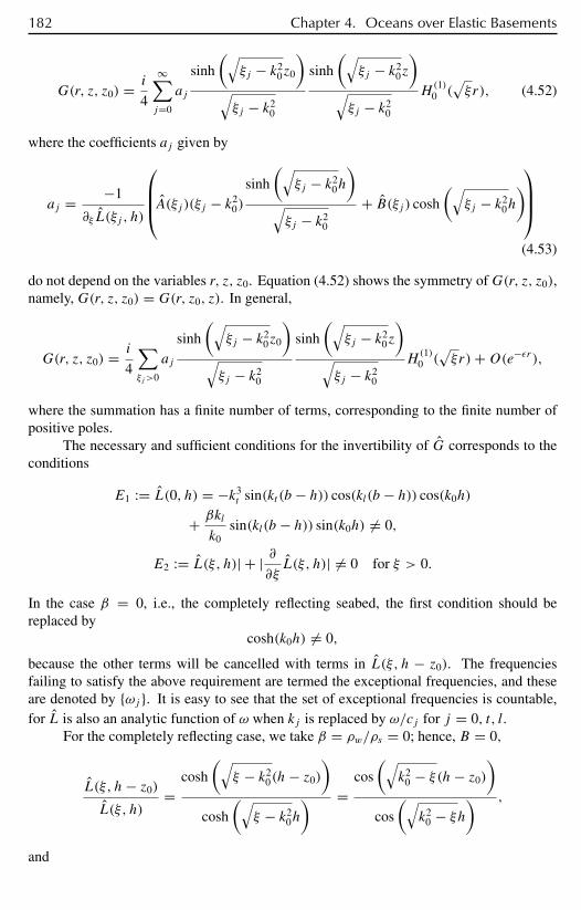
182 Chapter 4. Oceans over Elastic Basements
G(r, z, z0) = i
4
∞∑j=0
aj
sinh
(√ξj − k2
0z0
)√ξj − k2
0
sinh
(√ξj − k2
0z
)√ξj − k2
0
H(1)0 (
√ξr), (4.52)
where the coefficients aj given by
aj = −1
∂ξ L(ξj , h)
A(ξj )(ξj − k20)
sinh
(√ξj − k2
0h
)√ξj − k2
0
+ B(ξj ) cosh
(√ξj − k2
0h
)(4.53)
do not depend on the variables r, z, z0. Equation (4.52) shows the symmetry ofG(r, z, z0),namely, G(r, z, z0) = G(r, z0, z). In general,
G(r, z, z0) = i
4
∑ξj>0
aj
sinh
(√ξj − k2
0z0
)√ξj − k2
0
sinh
(√ξj − k2
0z
)√ξj − k2
0
H(1)0 (
√ξr)+O(e−εr ),
where the summation has a finite number of terms, corresponding to the finite number ofpositive poles.
The necessary and sufficient conditions for the invertibility of G corresponds to theconditions
E1 := L(0, h) = −k3t sin(kt (b − h)) cos(kl(b − h)) cos(k0h)
+ βkl
k0sin(kl(b − h)) sin(k0h) = 0,
E2 := L(ξ, h)| + | ∂∂ξL(ξ, h)| = 0 for ξ > 0.
In the case β = 0, i.e., the completely reflecting seabed, the first condition should bereplaced by
cosh(k0h) = 0,
because the other terms will be cancelled with terms in L(ξ, h − z0). The frequenciesfailing to satisfy the above requirement are termed the exceptional frequencies, and theseare denoted by ωj . It is easy to see that the set of exceptional frequencies is countable,for L is also an analytic function of ω when kj is replaced by ω/cj for j = 0, t, l.
For the completely reflecting case, we take β = ρw/ρs = 0; hence, B = 0,
L(ξ, h− z0)
L(ξ, h)=
cosh
(√ξ − k2
0(h− z0)
)cosh
(√ξ − k2
0h
) =cos
(√k2
0 − ξ(h− z0)
)cos
(√k2
0 − ξh) ,
and
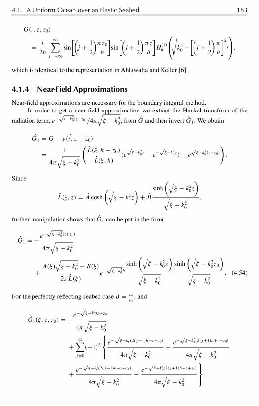
4.1. A Uniform Ocean over an Elastic Seabed 183
G(r, z, z0)
= i
2h
∞∑j=−∞
sin
[(j + 1
2
)πz0
h
]sin
[(j + 1
2
)πz
h
]H(1)0
√k20 −
[(j + 1
2
)π
h
]2
r
,which is identical to the representation in Ahluwalia and Keller [6].
4.1.4 Near-Field Approximations
Near-field approximations are necessary for the boundary integral method.In order to get a near-field approximation we extract the Hankel transform of the
radiation term, e−√ξ−k2
0 |z−z0|/4π√ξ − k2
0, from G and then invert G1. We obtain
G1 = ˆG− γ (r, z− z0)
= 1
4π√ξ − k2
0
(L(ξ, h− z0)
L(ξ, h)(e
√ξ−k2
0z − e−√ξ−k2
0z)− e√ξ−k2
0(z−z0)
).
Since
L(ξ, z) = A cosh
(√ξ − k2
0z
)+ B
sinh
(√ξ − k2
0z
)√ξ − k2
0
,
further manipulation shows that G1 can be put in the form
G1 = −e−√ξ−k2
0(z+z0)
4π√ξ − k2
0
+A(ξ)
√ξ − k2
0 − B(ξ)2πL(ξ)
e−√ξ−k2
0h
sinh
(√ξ − k2
0z
)√ξ − k2
0
sinh
(√ξ − k2
0z0
)√ξ − k2
0
. (4.54)
For the perfectly reflecting seabed case β = ρoρs
, and
G1(ξ, z, z0) = −e−√ξ−k2
0(z+z0)
4π√ξ − k2
0
+∞∑j=0
(−1)j
e−√ξ−k2
0(2(j+1)h−z−z0)
4π√ξ − k2
0
− e−√ξ−k2
0(2(j+1)h+z−z0)
4π√ξ − k2
0
+ e−√ξ−k2
0(2(j+1)h−z+z0)
4π√ξ − k2
0
− e−√ξ−k2
0(2(j+1)h−z+z0)
4π√ξ − k2
0
.
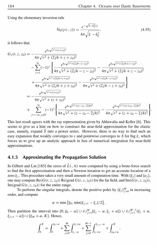
184 Chapter 4. Oceans over Elastic Basements
Using the elementary inversion rule
H0(γ (·, z)) = e−√ξ−k2
0 |z|
4π√ξ − k2
0
, (4.55)
it follows that
G1(r, z, z0) = − ek0
√r2+(z+z0)2
4π√r2 + (2jh+ z+ z0)2
−∞∑j=1
(−1)j
ek0
√r2+(2jh−z−z0)2
4π√r2 + (2jh− z− z0)2
− ek0
√r2+(2jh+z−z0)2
4π√r2 + (2jh+ z− z0)2
+ ek0
√r2+(2jh+z+z0)2
4π√r2 + (2jh+ z+ z0)2
− ek0
√r2+(2jh−z+z0)2
4π√r2 + (2jh− z+ z0)2
= − ek0
√r2+(z+z0)2
4π√r2 + (z+ z0)2
+∞∑
j=−∞,j =0
(−1)j
ek0
√r2+(z−z0−2jh)2
4π√r2 + (z− z0 − 2jh)2
− ek0
√r2+(z+z0−2jh)2
4π√r2 + (z+ z0 − 2jh)2
.
This last result agrees with the ray representation given by Ahluwalia and Keller [6]. Thisseems to give us a hint on how to construct the near-field approximation for the elasticcase, namely, expand S into a power series. However, there is no way to find such aneasy expansion that weakly converges to s and pointwise converges to S for big ξ , whichforces us to give up an analytic approach in lieu of numerical integration for near-fieldapproximations.
4.1.5 Approximating the Propagation Solution
In Gilbert and Lin [185] the zeros of L(·, h) were computed by using a brute-force searchto find the first approximation and then a Newton iteration to get an accurate location of azero ξj . This procedure takes a very small amount of computation time. With ξj and aj ,one may compute Re(G(r, z, z0)) Re(gradG(r, z, z0)) for the far field, and Im(G(r, z, z0)),Im(gradG(r, z, z0)) for the entire range.
To perform the singular integrals, denote the positive poles by ξj Mj=0 in increasingorder, and compute
α = minξ0,minξj+1 − ξj /2
.
Then partition the interval into [0, ξ0 − α] ∪ (∪Mj=1[ξj − α, ξj + α]) ∪ (∪M−1j=1 (ξj + α,
ξj+1 − α]) ∪ [ξM + α,K]. Hence,∫ K
0=∫ ξ0−α
0+
M∑j=0
∫ ξj+α
ξj−α+M−1∑j=0
∫ ξj+1−α
ξj+α+∫ K
ξM+α.
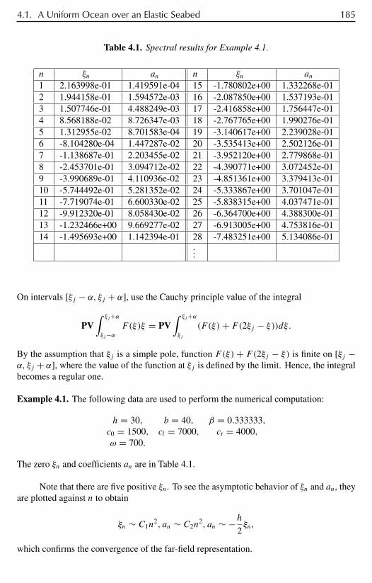
4.1. A Uniform Ocean over an Elastic Seabed 185
Table 4.1. Spectral results for Example 4.1.
n ξn an n ξn an1 2.163998e-01 1.419591e-04 15 -1.780802e+00 1.332268e-012 1.944158e-01 1.594572e-03 16 -2.087850e+00 1.537193e-013 1.507746e-01 4.488249e-03 17 -2.416858e+00 1.756447e-014 8.568188e-02 8.726347e-03 18 -2.767765e+00 1.990276e-015 1.312955e-02 8.701583e-04 19 -3.140617e+00 2.239028e-016 -8.104280e-04 1.447287e-02 20 -3.535413e+00 2.502126e-017 -1.138687e-01 2.203455e-02 21 -3.952120e+00 2.779868e-018 -2.453701e-01 3.094712e-02 22 -4.390771e+00 3.072452e-019 -3.990689e-01 4.110936e-02 23 -4.851361e+00 3.379413e-0110 -5.744492e-01 5.281352e-02 24 -5.333867e+00 3.701047e-0111 -7.719074e-01 6.600330e-02 25 -5.838315e+00 4.037471e-0112 -9.912320e-01 8.058430e-02 26 -6.364700e+00 4.388300e-0113 -1.232466e+00 9.669277e-02 27 -6.913005e+00 4.753816e-0114 -1.495693e+00 1.142394e-01 28 -7.483251e+00 5.134086e-01
...
On intervals [ξj − α, ξj + α], use the Cauchy principle value of the integral
PV∫ ξj+α
ξj−αF (ξ)ξ = PV
∫ ξj+α
ξj
(F (ξ)+ F(2ξj − ξ))dξ.
By the assumption that ξj is a simple pole, function F(ξ) + F(2ξj − ξ) is finite on [ξj −α, ξj + α], where the value of the function at ξj is defined by the limit. Hence, the integralbecomes a regular one.
Example 4.1. The following data are used to perform the numerical computation:
h = 30, b = 40, β = 0.333333,c0 = 1500, cl = 7000, ct = 4000,ω = 700.
The zero ξn and coefficients an are in Table 4.1.
Note that there are five positive ξn. To see the asymptotic behavior of ξn and an, theyare plotted against n to obtain
ξn ∼ C1n2, an ∼ C2n
2, an ∼ −h2ξn,
which confirms the convergence of the far-field representation.
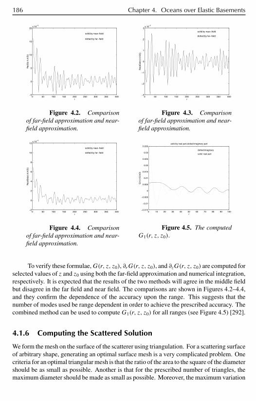
186 Chapter 4. Oceans over Elastic Basements
0 50 100 150 200 250 300 350 400−5
0
5
10
15
20x 10
−3
r
Re(
G(r
,h,h
/2))
solid:by near−field
dotted:by far−field
Figure 4.2. Comparisonof far-field approximation and near-field approximation.
0 50 100 150 200 250 300 350 400−3
−2
−1
0
1
2
3x 10
−3
r
Re(
dGdr
(r,h
,h/2
))
solid:by near−field
dotted:by far−field
Figure 4.3. Comparisonof far-field approximation and near-field approximation.
0 50 100 150 200 250 300 350 400−2
0
2
4
6
8
10
12x 10
−4
r
Re(
dGdz
(r,h
,h/2
))
solid:by near−field
dotted:by far−field
Figure 4.4. Comparisonof far-field approximation and near-field approximation.
0 10 20 30 40 50 60 70 80 90 100−0.015
−0.01
−0.005
0
0.005
0.01
0.015
0.02
0.025
0.03
0.035
solid: real part
dotted:imaginary
r
G1(
r,h/
2,h/
2)
solid:by real part,dotted:imaginary part
Figure 4.5. The computedG1(r, z, z0).
To verify these formulae,G(r, z, z0), ∂rG(r, z, z0), and ∂zG(r, z, z0) are computed forselected values of z and z0 using both the far-field approximation and numerical integration,respectively. It is expected that the results of the two methods will agree in the middle fieldbut disagree in the far field and near field. The comparisons are shown in Figures 4.2–4.4,and they confirm the dependence of the accuracy upon the range. This suggests that thenumber of modes used be range dependent in order to achieve the prescribed accuracy. Thecombined method can be used to computeG1(r, z, z0) for all ranges (see Figure 4.5) [292].
4.1.6 Computing the Scattered Solution
We form the mesh on the surface of the scatterer using triangulation. For a scattering surfaceof arbitrary shape, generating an optimal surface mesh is a very complicated problem. Onecriteria for an optimal triangular mesh is that the ratio of the area to the square of the diametershould be as small as possible. Another is that for the prescribed number of triangles, themaximum diameter should be made as small as possible. Moreover, the maximum variation

4.1. A Uniform Ocean over an Elastic Seabed 187
of the normal on a triangle should be made as small as possible. Hence, this is a multipleobjective optimization problem. See [185] for numerical data.
Let ˜∂ = ∪Tj be the approximation of the boundary ∂, where each Tj is a planartriangle. Moreover, let (xj , zj ) be the center of Tj , and nj the outward normal of Tj .Approximate the unknown function f on Tj by the constant fj . Then the boundary integralequation is discretized as (
−1
2I + A
)F + B = 0,
whereA = Aij Ni,j=1,
B = B1, B2, . . . , BN (,F = F1, F2, . . . , FN (,
with
Aij =∫Tj
∂
∂niG(|xi − x|, zi, z)dS(x,z),
Bi = ∂
∂niG(|xi − xs |, zi, zs).
To compute Aij , write G(|xi − x|, zi, z) as
G(|xi − x|, zi, z) = cos(k0r1)
r1+ Re(G1(|xi − x|, zi, z))+ i Im(G(|xi − x|, zi, z)),
where r1 = |xi − x, yi − y, zi − z|. The last two terms are regular, and their contributionstoAij can be approximated by using a routine quadrature formula for all i, j = 1, 2, . . . , N .For the first term, when i = j , since both (x, z) and (xj , zj ) are on Ti , xi−x, yi−y, zi−zis perpendicular to ni , and hence
∂
∂ni
cos(k0r1)
r1= 0.
For i = j , since r1 > 0, a quadrature method is used to compute∫Ti
∂
∂ni
cos(k0r1)
r1dS,
but when r1 is very small, a more accurate approximation may be needed.Due to the complicated wave guide fundamental singularity, the construction of the
stiff matrix A is a very time-consuming computation. This results from an essential difficultyof this problem, due to the interaction between the water column and the seabed. Comparedwith the scattering problems in the whole space, the computation of this step is sloweddown roughly by a factor proportional to the average number of modes multiplied by thetime for computing a Bessel function. Consequently, a parallel computation appears to bean efficient way to perform this calculation. Moreover, a number of parallelizations maybe used; for example, let each processor in a parallel computer be responsible for a portionof elements and use the iteration algorithm. The following generic scheme seems to beefficient [292].
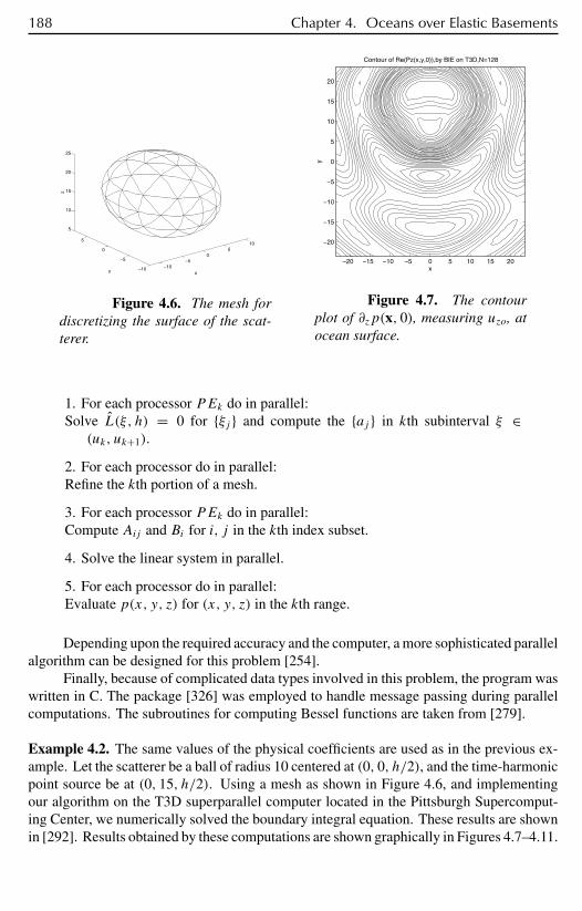
188 Chapter 4. Oceans over Elastic Basements
−10−5
05
10
−10
−5
0
5
5
10
15
20
25
xy
z
Figure 4.6. The mesh fordiscretizing the surface of the scat-terer.
−20 −15 −10 −5 0 5 10 15 20
−20
−15
−10
−5
0
5
10
15
20
x
y
Contour of Re(Pz(x,y,0)),by BIE on T3D,N=128
Figure 4.7. The contourplot of ∂zp(x, 0), measuring uzo, atocean surface.
1. For each processor PEk do in parallel:Solve L(ξ, h) = 0 for ξj and compute the aj in kth subinterval ξ ∈(uk, uk+1).
2. For each processor do in parallel:Refine the kth portion of a mesh.
3. For each processor PEk do in parallel:Compute Aij and Bi for i, j in the kth index subset.
4. Solve the linear system in parallel.
5. For each processor do in parallel:Evaluate p(x, y, z) for (x, y, z) in the kth range.
Depending upon the required accuracy and the computer, a more sophisticated parallelalgorithm can be designed for this problem [254].
Finally, because of complicated data types involved in this problem, the program waswritten in C. The package [326] was employed to handle message passing during parallelcomputations. The subroutines for computing Bessel functions are taken from [279].
Example 4.2. The same values of the physical coefficients are used as in the previous ex-ample. Let the scatterer be a ball of radius 10 centered at (0, 0, h/2), and the time-harmonicpoint source be at (0, 15, h/2). Using a mesh as shown in Figure 4.6, and implementingour algorithm on the T3D superparallel computer located in the Pittsburgh Supercomput-ing Center, we numerically solved the boundary integral equation. These results are shownin [292]. Results obtained by these computations are shown graphically in Figures 4.7–4.11.
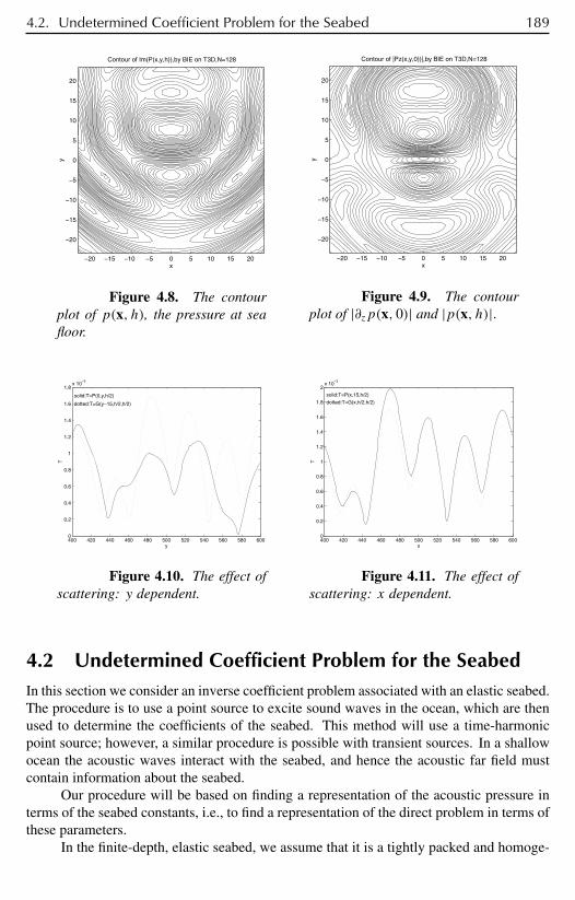
4.2. Undetermined Coefficient Problem for the Seabed 189
−20 −15 −10 −5 0 5 10 15 20
−20
−15
−10
−5
0
5
10
15
20
x
yContour of Im(P(x,y,h)),by BIE on T3D,N=128
Figure 4.8. The contourplot of p(x, h), the pressure at seafloor.
−20 −15 −10 −5 0 5 10 15 20
−20
−15
−10
−5
0
5
10
15
20
x
y
Contour of |Pz(x,y,0))|,by BIE on T3D,N=128
Figure 4.9. The contourplot of |∂zp(x, 0)| and |p(x, h)|.
400 420 440 460 480 500 520 540 560 580 6000
0.2
0.4
0.6
0.8
1
1.2
1.4
1.6
1.8x 10
−3
y
T
solid:T=P(0,y,h/2)
dotted:T=G(y−15,h/2,h/2)
Figure 4.10. The effect ofscattering: y dependent.
400 420 440 460 480 500 520 540 560 580 6000
0.2
0.4
0.6
0.8
1
1.2
1.4
1.6
1.8
2x 10
−3
x
T
solid:T=P(x,15,h/2)
dotted:T=G(x,h/2,h/2)
Figure 4.11. The effect ofscattering: x dependent.
4.2 Undetermined Coefficient Problem for the SeabedIn this section we consider an inverse coefficient problem associated with an elastic seabed.The procedure is to use a point source to excite sound waves in the ocean, which are thenused to determine the coefficients of the seabed. This method will use a time-harmonicpoint source; however, a similar procedure is possible with transient sources. In a shallowocean the acoustic waves interact with the seabed, and hence the acoustic far field mustcontain information about the seabed.
Our procedure will be based on finding a representation of the acoustic pressure interms of the seabed constants, i.e., to find a representation of the direct problem in terms ofthese parameters.
In the finite-depth, elastic seabed, we assume that it is a tightly packed and homoge-
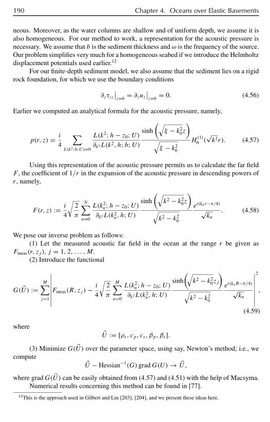
190 Chapter 4. Oceans over Elastic Basements
neous. Moreover, as the water columns are shallow and of uniform depth, we assume it isalso homogeneous. For our method to work, a representation for the acoustic pressure isnecessary. We assume that b is the sediment thickness and ω is the frequency of the source.Our problem simplifies very much for a homogeneous seabed if we introduce the Helmholtzdisplacement potentials used earlier.12
For our finite-depth sediment model, we also assume that the sediment lies on a rigidrock foundation, for which we use the boundary conditions
∂zτzz∣∣z=b = ∂zuz
∣∣z=b = 0. (4.56)
Earlier we computed an analytical formula for the acoustic pressure, namely,
p(r, z) = i
4
∑L(k2;h;U)=0
L(k2;h− z0;U)∂k2L(k2, h; b;U)
sinh
(√ξ − k2
0z
)√ξ − k2
0
H(1)0 (
√k2r). (4.57)
Using this representation of the acoustic pressure permits us to calculate the far fieldF , the coefficient of 1/r in the expansion of the acoustic pressure in descending powers ofr , namely,
F(r, z) := i
4
√2
π
N∑n=0
L(k2n;h− z0;U)
∂k2L(k2n, h;U)
sinh
(√k2 − k2
0z
)√k2 − k2
0
ei(knr−π/4)√kn
. (4.58)
We pose our inverse problem as follows:(1) Let the measured acoustic far field in the ocean at the range r be given as
Fmeas(r, zj ), j = 1, 2, . . . ,M .(2) Introduce the functional
G( $U) :=M∑j=1
∣∣∣∣∣∣∣∣Fmeas(R, zj )− i
4
√2
π
M∑n=0
L(k2n;h− z0;U)
∂k2L(k2n, h;U)
sinh
(√k2 − k2
0zj
)√k2 − k2
0
ei(knR−π/4)√kn
∣∣∣∣∣∣∣∣2
,
(4.59)
where$U := [ρs, cp, cs, βp, βs].
(3) Minimize G( $U) over the parameter space, using say, Newton’s method; i.e., wecompute
$U − Hessian−1(G) gradG(U)→ $U,where gradG( $U) can be easily obtained from (4.57) and (4.51) with the help of Macsyma.
Numerical results concerning this method can be found in [77].12This is the approach used in Gilbert and Lin [203], [204], and we present these ideas here.
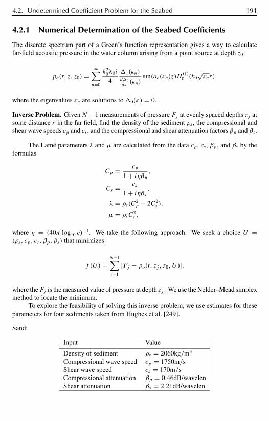
4.2. Undetermined Coefficient Problem for the Seabed 191
4.2.1 Numerical Determination of the Seabed Coefficients
The discrete spectrum part of a Green’s function representation gives a way to calculatefar-field acoustic pressure in the water column arising from a point source at depth z0:
po(r, z, z0) =∞∑n=0
k20λ0i
4
1(κn)d0dκ(κn)
sin(ao(κn)z)H(1)0 (k0
√κnr),
where the eigenvalues κn are solutions to 0(κ) = 0.
Inverse Problem. GivenN − 1 measurements of pressure Fj at evenly spaced depths zj atsome distance r in the far field, find the density of the sediment ρs , the compressional andshear wave speeds cp and cs , and the compressional and shear attenuation factors βp and βs .
The Lamé parameters λ and µ are calculated from the data cp, cs , βp, and βs by theformulas
Cp = cp
1 + iηβp ,
Cs = cs
1 + iηβs ,λ = ρs(C
2p − 2C2
s ),
µ = ρsC2s ,
where η = (40π log10 e)−1. We take the following approach. We seek a choice U =
(ρs, cp, cs, βp, βs) that minimizes
f (U) =N−1∑i=1
|Fj − po(r, zj , z0, U)|,
where theFj is the measured value of pressure at depth zj . We use the Nelder–Mead simplexmethod to locate the minimum.
To explore the feasibility of solving this inverse problem, we use estimates for theseparameters for four sediments taken from Hughes et al. [249].
Sand:
Input Value
Density of sediment ρs = 2060kg/m3
Compressional wave speed cp = 1750m/sShear wave speed cs = 170m/sCompressional attenuation βp = 0.46dB/wavelenShear attenuation βs = 2.21dB/wavelen
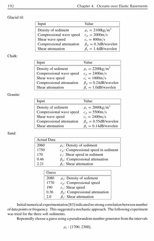
192 Chapter 4. Oceans over Elastic Basements
Glacial til:
Input Value
Density of sediment ρs = 2100kg/m3
Compressional wave speed cp = 2000m/sShear wave speed cs = 800m/sCompressional attenuation βp = 0.3dB/wavelenShear attenuation βs = 1.4dB/wavelen
Chalk:
Input Value
Density of sediment ρs = 2200kg/m3
Compressional wave speed cp = 2400m/sShear wave speed cs = 1000m/sCompressional attenuation βp = 0.24dB/wavelenShear attenuation βs = 1.0dB/wavelen
Granite:
Input Value
Density of sediment ρs = 2600kg/m3
Compressional wave speed cp = 5500m/sShear wave speed cs = 2400m/sCompressional attenuation βp = 0.55dB/wavelenShear attenuation βs = 0.14dB/wavelen
Sand:
Actual Data
2060 ρs : Density of sediment1750 cp: Compressional speed in sediment170 cs : Shear speed in sediment0.46 βp: Compressional attenuation2.21 βs : Shear attenuation
Guess
2080 ρs : Density of sediment1770 cp: Compressional speed190 cs : Shear speed0.36 βp: Compressional attenuation2.0 βs : Shear attenuation
Initial numerical experimentation [83] indicated no strong correlation between numberof data points or frequency. This suggested a stochastic approach. The following experimentwas tried for the three soft sediments.
Repeatedly choose a guess using a pseudorandom number generator from the intervals
ρs : [1700, 2300],
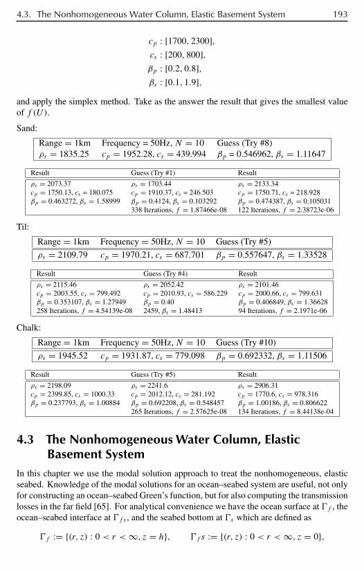
4.3. The Nonhomogeneous Water Column, Elastic Basement System 193
cp : [1700, 2300],cs : [200, 800],βp : [0.2, 0.8],βs : [0.1, 1.9],
and apply the simplex method. Take as the answer the result that gives the smallest valueof f (U).
Sand:
Range = 1km Frequency = 50Hz, N = 10 Guess (Try #8)ρs = 1835.25 cp = 1952.28, cs = 439.994 βp = 0.546962, βs = 1.11647
Result Guess (Try #1) Result
ρs = 2073.37 ρs = 1703.44 ρs = 2133.34cp = 1750.13, cs = 180.075 cp = 1910.37, cs = 246.503 cp = 1750.71, cs = 218.928βp = 0.463272, βs = 1.58999 βp = 0.4124, βs = 0.103292 βp = 0.474387, βs = 0.105031
338 Iterations, f = 1.87466e-08 122 Iterations, f = 2.38723e-06
Til:
Range = 1km Frequency = 50Hz, N = 10 Guess (Try #5)
ρs = 2109.79 cp = 1970.21, cs = 687.701 βp = 0.557647, βs = 1.33528
Result Guess (Try #4) Result
ρs = 2115.46 ρs = 2052.42 ρs = 2101.46cp = 2003.55, cs = 799.492 cp = 2010.93, cs = 586.229 cp = 2000.66, cs = 799.631βp = 0.353107, βs = 1.27949 βp = 0.40 βp = 0.406849, βs = 1.36628258 Iterations, f = 4.54139e-08 2459, βs = 1.48413 94 Iterations, f = 2.1971e-06
Chalk:
Range = 1km Frequency = 50Hz, N = 10 Guess (Try #10)
ρs = 1945.52 cp = 1931.87, cs = 779.098 βp = 0.692332, βs = 1.11506
Result Guess (Try #5) Result
ρs = 2198.09 ρs = 2241.6 ρs = 2906.31cp = 2399.85, cs = 1000.33 cp = 2012.12, cs = 281.192 cp = 1770.6, cs = 978.316βp = 0.237793, βs = 1.00884 βp = 0.692208, βs = 0.548457 βp = 1.00186, βs = 0.806622
265 Iterations, f = 2.57625e-08 134 Iterations, f = 8.44138e-04
4.3 The Nonhomogeneous Water Column, ElasticBasement System
In this chapter we use the modal solution approach to treat the nonhomogeneous, elasticseabed. Knowledge of the modal solutions for an ocean–seabed system are useful, not onlyfor constructing an ocean–seabed Green’s function, but for also computing the transmissionlosses in the far field [65]. For analytical convenience we have the ocean surface at f , theocean–seabed interface at f s , and the seabed bottom at s which are defined as
f := (r, z) : 0 < r <∞, z = h, f s := (r, z) : 0 < r <∞, z = 0,
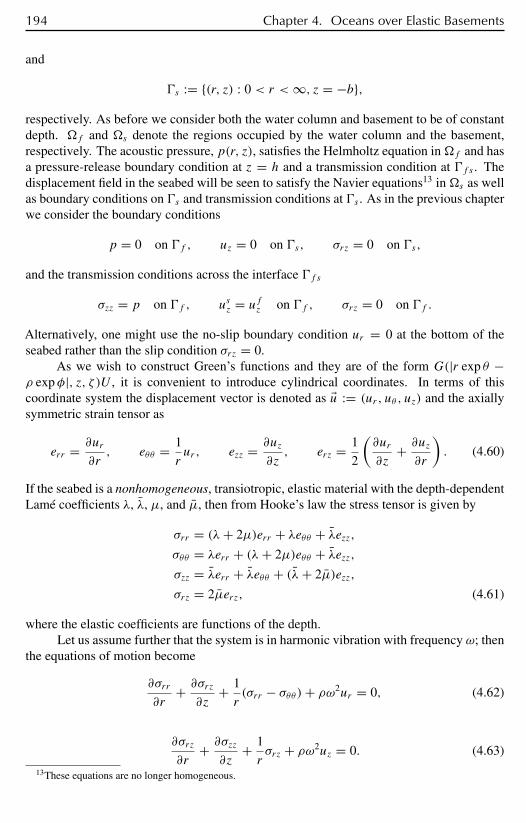
194 Chapter 4. Oceans over Elastic Basements
and
s := (r, z) : 0 < r <∞, z = −b,respectively. As before we consider both the water column and basement to be of constantdepth. f and s denote the regions occupied by the water column and the basement,respectively. The acoustic pressure, p(r, z), satisfies the Helmholtz equation inf and hasa pressure-release boundary condition at z = h and a transmission condition at f s . Thedisplacement field in the seabed will be seen to satisfy the Navier equations13 ins as wellas boundary conditions on s and transmission conditions at s . As in the previous chapterwe consider the boundary conditions
p = 0 on f , uz = 0 on s, σrz = 0 on s,
and the transmission conditions across the interface f s
σzz = p on f , usz = ufz on f , σrz = 0 on f .
Alternatively, one might use the no-slip boundary condition ur = 0 at the bottom of theseabed rather than the slip condition σrz = 0.
As we wish to construct Green’s functions and they are of the form G(|r exp θ −ρ expφ|, z, ζ )U , it is convenient to introduce cylindrical coordinates. In terms of thiscoordinate system the displacement vector is denoted as $u := (ur , uθ , uz) and the axiallysymmetric strain tensor as
err = ∂ur
∂r, eθθ = 1
rur , ezz = ∂uz
∂z, erz = 1
2
(∂ur
∂z+ ∂uz
∂r
). (4.60)
If the seabed is a nonhomogeneous, transiotropic, elastic material with the depth-dependentLamé coefficients λ, λ, µ, and µ, then from Hooke’s law the stress tensor is given by
σrr = (λ+ 2µ)err + λeθθ + λezz,σθθ = λerr + (λ+ 2µ)eθθ + λezz,σzz = λerr + λeθθ + (λ+ 2µ)ezz,
σrz = 2µerz, (4.61)
where the elastic coefficients are functions of the depth.Let us assume further that the system is in harmonic vibration with frequency ω; then
the equations of motion become
∂σrr
∂r+ ∂σrz
∂z+ 1
r(σrr − σθθ )+ ρω2ur = 0, (4.62)
∂σrz
∂r+ ∂σzz
∂z+ 1
rσrz + ρω2uz = 0. (4.63)
13These equations are no longer homogeneous.
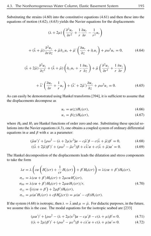
4.3. The Nonhomogeneous Water Column, Elastic Basement System 195
Substituting the strains (4.60) into the constitutive equations (4.61) and then these into theequations of motion (4.62), (4.63) yields the Navier equations for the displacements
(λ+ 2µ)
(∂2ur
∂r2+ 1
r
∂ur
∂r− 1
r2ur
)
+ (λ+ µ) ∂2uz
∂r∂z+ µ∂zzur + µ′
(∂ur
∂z+ ∂ruz
)+ ρω2ur = 0, (4.64)
(λ+ 2µ)∂2uz
∂z2+ (λ+ µ)
(∂rzur + 1
r
∂ur
∂z
)+ µ
(∂2uz
∂r2+ 1
r
∂uz
∂r
)
+ λ′(∂ur
∂r+ 1
rur
)+ (λ′ + 2µ′)
∂uz
∂z+ ρω2uz = 0. (4.65)
As can easily be demonstrated using Hankel transforms [394], it is sufficient to assume thatthe displacements decompose as
ur = α(z)H1(cr), (4.66)
uz = β(z)H0(cr), (4.67)
whereH0 andH1 are Hankel functions of order zero and one. Substituting these special so-lutions into the Navier equations (4.3), one obtains a coupled system of ordinary differentialequations in α and β with κ as a parameter:
(µα′)′ + [ρω2 − (λ+ 2µ)c2]α − cµ′β − c(λ+ µ)β ′ = 0, (4.68)
((λ+ 2µ)β ′)′ + (ρω2 − µc2)β + cλ′α + c(λ+ µ)α′ = 0. (4.69)
The Hankel decomposition of the displacements leads the dilatation and stress componentsto take the form
λe = λ
(cα
(H ′
1(cr)+1
crH1(cr)
)+ β ′H0(cr)
)= λ(cα + β ′)H0(cr),
σrr = λ(cα + β ′)H0(cr)+ 2µcαH ′1(cr),
σθθ = λ(cα + β ′)H0(cr)+ 2µαH1(cr)/r, (4.70)
σzz = (λ(cα + β ′)+ 2µβ ′)H0(cr),
σrz = µ(α′H1(cr)+ cβH ′0(cr)) = µ(α′ − cβ)H1(cr).
If the system (4.68) is isotropic, then λ = λ andµ = µ. For didactic purposes, in the future,we assume this is the case. The modal equations for the isotropic seabed are [233]
(µα′)′ + [ρω2 − (λ+ 2µ)c2]α − cµ′β − c(λ+ µ)β ′= 0, (4.71)
((λ+ 2µ)β ′)′ + (ρω2 − µc2)β + cλ′α + c(λ+ µ)α′= 0. (4.72)
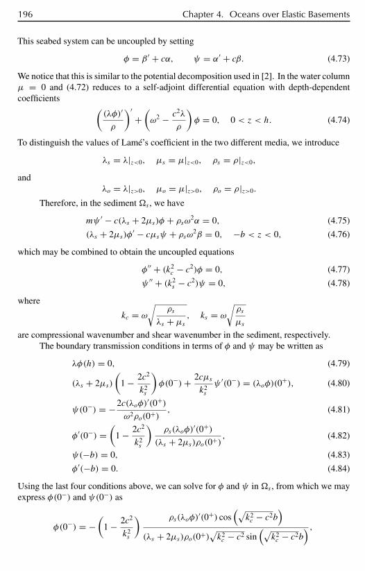
196 Chapter 4. Oceans over Elastic Basements
This seabed system can be uncoupled by setting
φ = β ′ + cα, ψ = α′ + cβ. (4.73)
We notice that this is similar to the potential decomposition used in [2]. In the water columnµ = 0 and (4.72) reduces to a self-adjoint differential equation with depth-dependentcoefficients (
(λφ)′
ρ
)′+(ω2 − c2λ
ρ
)φ = 0, 0 < z < h. (4.74)
To distinguish the values of Lamé’s coefficient in the two different media, we introduce
λs = λ|z<0, µs = µ|z<0, ρs = ρ|z<0,
andλo = λ|z>0, µo = µ|z>0, ρo = ρ|z>0.
Therefore, in the sediment s , we have
mψ ′ − c(λs + 2µs)φ + ρsω2α = 0, (4.75)
(λs + 2µs)φ′ − cµsψ + ρsω2β = 0, −b < z < 0, (4.76)
which may be combined to obtain the uncoupled equations
φ′′ + (k2c − c2)φ = 0, (4.77)
ψ ′′ + (k2s − c2)ψ = 0, (4.78)
where
kc = ω
√ρs
λs + µs , ks = ω
√ρs
µs
are compressional wavenumber and shear wavenumber in the sediment, respectively.The boundary transmission conditions in terms of φ and ψ may be written as
λφ(h) = 0, (4.79)
(λs + 2µs)
(1 − 2c2
k2s
)φ(0−)+ 2cµs
k2s
ψ ′(0−) = (λoφ)(0+), (4.80)
ψ(0−) = −2c(λoφ)′(0+)ω2ρo(0+)
, (4.81)
φ′(0−) =(
1 − 2c2
k2s
)ρs(λoφ)
′(0+)(λs + 2µs)ρo(0+)
, (4.82)
ψ(−b) = 0, (4.83)
φ′(−b) = 0. (4.84)
Using the last four conditions above, we can solve for φ and ψ in s , from which we mayexpress φ(0−) and ψ(0−) as
φ(0−) = −(
1 − 2c2
k2s
) ρs(λoφ)′(0+) cos
(√k2c − c2b
)(λs + 2µs)ρo(0+)
√k2c − c2 sin
(√k2c − c2b
) ,
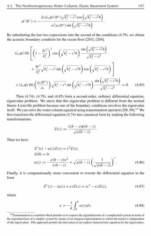
4.3. The Nonhomogeneous Water Column, Elastic Basement System 197
ψ ′(0−) = −2c(λoφ)′(0+)
√k2s − c2 cos
(√k2s − c2b
)ω2ρo(0+) sin
(√k2s − c2b
) .
By substituting the last two expressions into the second of the conditions (4.79), we obtainthe acoustic boundary condition for the ocean floor [203], [204].
(λoφ)′(0)
(1 − 2c2
k2s
)2
cos
(√k2c − c2b
) sin(√k2s − c2b
)√k2s − c2
+ 4c2
k4s
√k2c − c2 sin
(√k2c − c2b
)cos
(√k2s − c2b
)+ (λoφ) (0)
(ρo(0+)ρs
)√k2c − c2 sin
(√k2c − c2b
) sin(√k2s − c2b
)√k2s − c2
= 0. (4.85)
Then (4.74), (4.79), and (4.85) form a second-order, ordinary differential equation,eigenvalue problem. We stress that this eigenvalue problem is different from the normalSturm–Liouville problem because one of the boundary conditions involves the eigenvalueitself. We can solve the water column equation using transmutation operators [98, 99].14 Wefirst transform the differential equation (4.74) into canonical form by making the followingtransformations:
Z(z) := λ(h− z)φ(h− z)√ρ(h− z) .
Then we have
Z′′(z)− a(z)Z(z) = c2Z(z),
Z(0) = 0,
a(z) := −ρ(h− z)ω2
λ(h− z) +√ρ(h− z)
(1√
ρ(h− z))′′. (4.86)
Finally, it is computationally more convenient to rewrite the differential equation in theform
Z′′(z)− (a(z)+ κ)Z(z) = (c2 − κ)Z(z), (4.87)
where
κ = −1
h
∫ h
0a(τ)dτ. (4.88)
14Transmutation is a method which permits us to express the eigenfunctions of a complicated system in terms ofthe eigenfunctions of a simpler system by means of an integral representation in which the kernel is independentof the eigenvalues. This approach permits the derivation of an explicit characteristic equation for the eigenvalues.
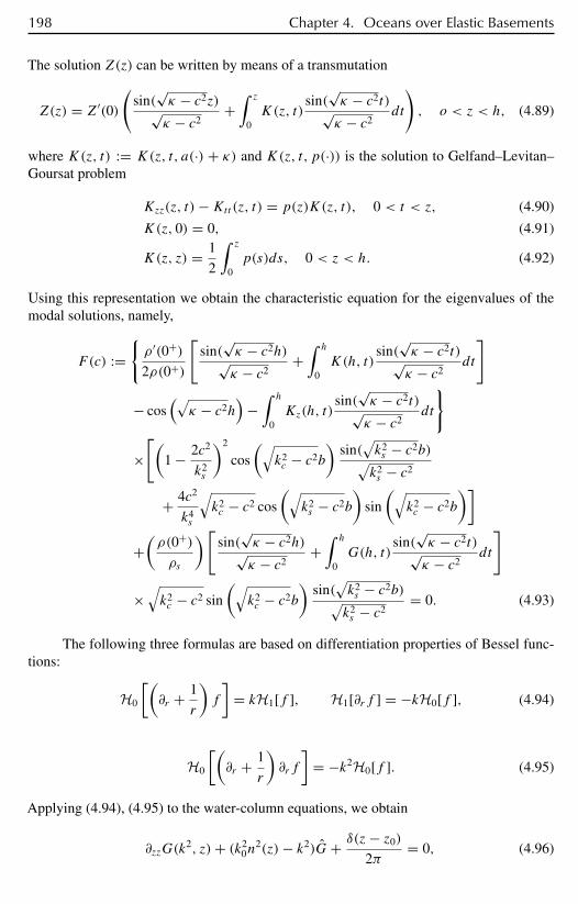
198 Chapter 4. Oceans over Elastic Basements
The solution Z(z) can be written by means of a transmutation
Z(z) = Z′(0)
(sin(
√κ − c2z)√κ − c2
+∫ z
0K(z, t)
sin(√κ − c2t)√κ − c2
dt
), o < z < h, (4.89)
where K(z, t) := K(z, t, a(·) + κ) and K(z, t, p(·)) is the solution to Gelfand–Levitan–Goursat problem
Kzz(z, t)−Ktt (z, t) = p(z)K(z, t), 0 < t < z, (4.90)
K(z, 0) = 0, (4.91)
K(z, z) = 1
2
∫ z
0p(s)ds, 0 < z < h. (4.92)
Using this representation we obtain the characteristic equation for the eigenvalues of themodal solutions, namely,
F(c) :=ρ ′(0+)2ρ(0+)
[sin(
√κ − c2h)√κ − c2
+∫ h
0K(h, t)
sin(√κ − c2t)√κ − c2
dt
]
− cos(√κ − c2h
)−∫ h
0Kz(h, t)
sin(√κ − c2t)√κ − c2
dt
×[(
1 − 2c2
k2s
)2
cos
(√k2c − c2b
)sin(
√k2s − c2b)√
k2s − c2
+ 4c2
k4s
√k2c − c2 cos
(√k2s − c2b
)sin
(√k2c − c2b
)]+(ρ(0+)ρs
)[sin(
√κ − c2h)√κ − c2
+∫ h
0G(h, t)
sin(√κ − c2t)√κ − c2
dt
]
×√k2c − c2 sin
(√k2c − c2b
)sin(
√k2s − c2b)√
k2s − c2
= 0. (4.93)
The following three formulas are based on differentiation properties of Bessel func-tions:
H0
[(∂r + 1
r
)f
]= kH1[f ], H1[∂rf ] = −kH0[f ], (4.94)
H0
[(∂r + 1
r
)∂rf
]= −k2H0[f ]. (4.95)
Applying (4.94), (4.95) to the water-column equations, we obtain
∂zzG(k2, z)+ (k2
0n2(z)− k2)G+ δ(z− z0)
2π= 0, (4.96)

4.3. The Nonhomogeneous Water Column, Elastic Basement System 199
ω2ρwuzo + ∂zG = 0, 0 < z < h. (4.97)
Applying (4.94) to the dilatation and the stress components, we get
H0[e] = k2ur + ∂zuz, (4.98)
H0[σzz] = λ(k2ur + ∂zuz)+ 2µ∂zuz, (4.99)
H1[σrz] = µk(∂zur − uz), (4.100)
H0[σrr ] = (λ+ 2µ)k2ur + λ∂zuz − 2µH0
[urr
]. (4.101)
Letting H1 act on (4.62), H0 on (4.63), and applying (4.94) to them, we obtain
−kH0[σrr ] + ∂zH1[σrz] − 2kµH0
[urr
]+ ω2ρkur = 0. (4.102)
kH1[σrz] + ∂zH0[σzz] + ω2ρuz = 0. (4.103)
Inserting (4.99)–(4.101) into (4.102)–(4.103) yields
∂z(µ∂zur )+ [ρω2 − (λ+ 2µ)k2]ur − µ′uz − (λ+ µ)∂zuz = 0, (4.104)
∂z((λ+ 2µ)∂zuz)+ (ρω2 − µk2)uz + k2λ′ur + k2(λ+ µ)∂zur = 0. (4.105)
Similarly, the boundary transmission conditions are transformed into
G∣∣z=0 = 0, (4.106)
uzo|z=h− = uz|z=h+ , (4.107)
G|z=h− = [λ(k2ur + ∂uz)+ 2µ∂zu]∣∣∣∣z=h+
, (4.108)
[∂zur − uz]∣∣∣∣z=h+
= 0, (4.109)
∂zur
∣∣∣∣z=b
= uz
∣∣∣∣z=b
= 0. (4.110)
The equations (4.96), (4.97), (4.104)–(4.110) form the Hankel-transformed ocean–seabedsystem. In the case of constant coefficients, we can solve it explicitly. If the coefficientsare variable, we can construct a solution to this system and implement it numerically.
For the case of depth-dependent coefficients, we associate the initial value problemwith the Hankel-transformed modal equations for the water column,
X′′(z)+ (k20n
2(z)− k2)X(z) = 0, z ∈ (0, h), (4.111)
X(c) = 0, X′(c) = 1. (4.112)
The Green’s function of (4.112) can be constructed using undetermined coefficients. As theGreen’s function, G(k2, z), satisfies (4.96)–(4.106), it must be expressed as
G(k2, z) = 1
2π[C1X(k
2, z, 0)−H(z− z0)X(k2, z, z0)] (4.113)
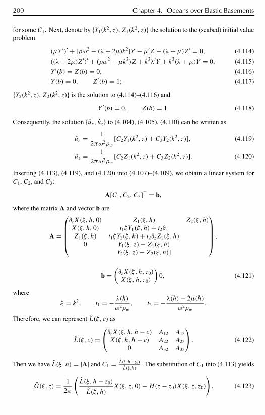
200 Chapter 4. Oceans over Elastic Basements
for someC1. Next, denote by Y1(k2, z), Z1(k
2, z) the solution to the (seabed) initial valueproblem
(µY ′)′ + [ρω2 − (λ+ 2µ)k2]Y − µ′Z − (λ+ µ)Z′ = 0, (4.114)
((λ+ 2µ)Z′)′ + (ρω2 − µk2)Z + k2λ′Y + k2(λ+ µ)Y = 0, (4.115)
Y ′(b) = Z(b) = 0, (4.116)
Y (b) = 0, Z′(b) = 1; (4.117)
Y2(k2, z), Z2(k
2, z) is the solution to (4.114)–(4.116) and
Y ′(b) = 0, Z(b) = 1. (4.118)
Consequently, the solution ur , uz to (4.104), (4.105), (4.110) can be written as
ur = 1
2πω2ρw[C2Y1(k
2, z)+ C3Y2(k2, z)], (4.119)
uz = 1
2πω2ρw[C2Z1(k
2, z)+ C3Z2(k2, z)]. (4.120)
Inserting (4.113), (4.119), and (4.120) into (4.107)–(4.109), we obtain a linear system forC1, C2, and C3:
A[C1, C2, C3]( = b,
where the matrix A and vector b are
A =
∂zX(ξ, h, 0) Z1(ξ, h) Z2(ξ, h)
X(ξ, h, 0) t1ξY1(ξ, h)+ t2∂zZ1(ξ, h) t1ξY2(ξ, h)+ t2∂zZ2(ξ, h)
0 Y1(ξ, z)− Z1(ξ, h)
Y2(ξ, z)− Z2(ξ, h)]
,
b =(∂zX(ξ, h, z0)
X(ξ, h, z0)
)0, (4.121)
where
ξ = k2, t1 = − λ(h)
ω2ρw, t2 = −λ(h)+ 2µ(h)
ω2ρw.
Therefore, we can represent L(ξ, c) as
L(ξ, c) =∂zX(ξ, h, h− c) A12 A13
X(ξ, h, h− c) A22 A23
0 A32 A33
. (4.122)
Then we have L(ξ, h) = |A| and C1 = L(ξ,h−z0)
L(ξ,h). The substitution of C1 into (4.113) yields
G(ξ, z) = 1
2π
(L(ξ, h− z0)
L(ξ, h)X(ξ, z, 0)−H(z− z0)X(ξ, z, z0)
). (4.123)
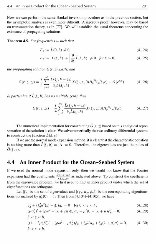
4.4. An Inner Product for the Ocean–Seabed System 201
Now we can perform the same Hankel inversion procedure as in the previous section, butthe asymptotic analysis is even more difficult. A rigorous proof, however, may be basedon transmutation theory, as in [77]. We will establish the usual theorems concerning theexistence of propagating solutions.
Theorem 4.5. For frequencies ω such that
E1 := L(0, h) = 0, (4.124)
E2 := |L(ξ, h)| +∣∣∣∣ ∂∂ξ L(ξ, h)
∣∣∣∣ = 0 for ξ > 0, (4.125)
the propagating solution G(r, z) exists, and
G(r, z, z0) = i
4
M∑j=0
L(ξj , h− z0)
∂ξ L(ξj , h)X(ξj , z, 0)H
(1)0 (
√ξj r)+O(eε2r ). (4.126)
In particular, if L(ξ, h) has no multiple zeros, then
G(r, z, z0) = i
4
∞∑j=0
L(ξj , h− z0)
∂ξ L(ξj , h)X(ξj , z, 0)H
(1)0 (
√ξj r). (4.127)
The numerical implementation for constructingG(r, z) based on this analytical repre-sentation of the solution is clear. We solve numerically the two ordinary differential systemsto construct the function L(ξ, c).
If we use the normal mode expansion method, it is clear that the characteristic equationis nothing more than L(ξ, h) = |A| = 0. Therefore, the eigenvalues are just the poles ofG(ξ, z).
4.4 An Inner Product for the Ocean–Seabed SystemIf we used the normal mode expansion only, then we would not know that the Fourier
expansion had the coefficients L(ξj ,h−z0)
∂ξ L(ξj ,h)as indicated above. To construct the coefficients
from the eigenvalue problem, we first need to find an inner product under which the set ofeigenfunctions are orthogonal.
Let ξn be the set of eigenvalues and (gn, αn, βn) be the corresponding eigenfunc-tions normalized by g′
n(0) = 1. Then from (4.104)–(4.105), we have
g′′n + (k2
0n2(z)− ξn)gn = 0 for 0 < z < h, (4.128)
(µα′n)
′ + [ρω2 − (λ+ 2µ)ξn]αn − µ′βn − (λ+ µ)β ′n = 0, (4.129)
h < z < b,
((λ+ 2µ)β ′n)
′ + (ρω2 − µξ 2n )βn + ξnλ′αn + ξn(λ+ µ)α′
n = 0, (4.130)
h < z < b,
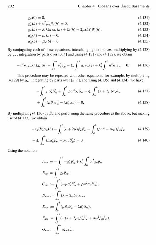
202 Chapter 4. Oceans over Elastic Basements
gn(0) = 0, (4.131)
g′n(h)+ ω2ρwβn(h) = 0, (4.132)
gn(h) = ξnλ(h)αn(h)+ (λ(h)+ 2µ(h))β ′n(h), (4.133)
α′n(h)− βn(h) = 0, (4.134)
α′n(b) = βn(b) = 0. (4.135)
By conjugating each of these equations, interchanging the indices, multiplying by (4.128)by gm, integration by parts over [0, h] and using (4.131) and (4.132), we obtain
−ω2ρwβn(h)gm(h)−∫ h
0g′ng
′m − ξn
∫ h
0gngm(z)+ k2
0
∫ h
0n2gngm = 0. (4.136)
This procedure may be repeated with other equations; for example, by multiplying(4.129) by αm, integrating by parts over [h, b], and using (4.135) and (4.134), we have
−∫ b
h
µα′nα
′m +
∫ b
h
ρω2αnαm − ξn∫ b
h
(λ+ 2µ)αnαm (4.137)
+∫ b
h
(µβnα′m − λβ ′
nαm) = 0. (4.138)
By multiplying (4.130) by βm and performing the same procedure as the above, but makinguse of (4.133), we obtain
−gn(h)βm(h)−∫ b
h
(λ+ 2µ)β ′nβ
′m +
∫ b
h
(ρω2 − µξn)βnβm (4.139)
+ ξn∫ b
h
(µα′nβm − λαnβ ′
m) = 0. (4.140)
Using the notation
Anm = −∫ h
0−g′
ng′m + k2
0
∫ h
0n2gngm,
Bnm =∫ h
0gngm,
Cnm :=∫ b
h
(−µα′nα
′m + ρω2αnαm),
Dnm :=∫ b
h
(λ+ 2µ)αnαm,
Enm :=∫ b
h
(µβnα′m − λβ ′
nαm),
Fnm :=∫ b
h
(−(λ+ 2µ)β ′nβ
′m + ρω2βnβm),
Gnm :=∫ b
h
µβnβm,
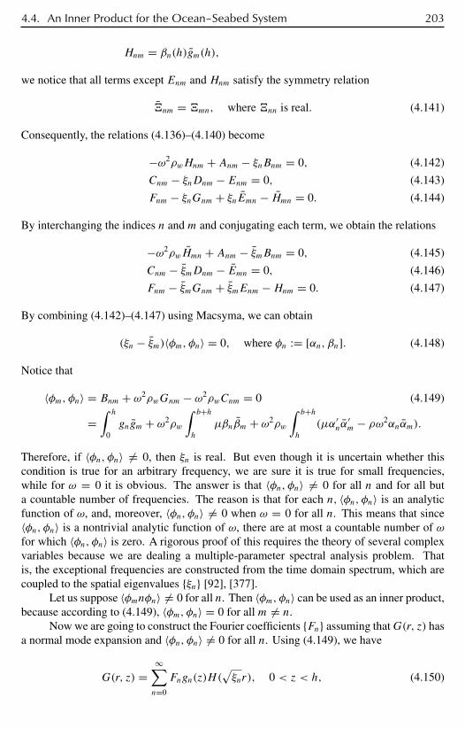
4.4. An Inner Product for the Ocean–Seabed System 203
Hnm = βn(h)gm(h),
we notice that all terms except Enm and Hnm satisfy the symmetry relation
nm = mn, where nn is real. (4.141)
Consequently, the relations (4.136)–(4.140) become
−ω2ρwHnm + Anm − ξnBnm = 0, (4.142)
Cnm − ξnDnm − Enm = 0, (4.143)
Fnm − ξnGnm + ξnEmn − Hmn = 0. (4.144)
By interchanging the indices n and m and conjugating each term, we obtain the relations
−ω2ρwHmn + Anm − ξmBnm = 0, (4.145)
Cnm − ξmDnm − Emn = 0, (4.146)
Fnm − ξmGnm + ξmEnm −Hnm = 0. (4.147)
By combining (4.142)–(4.147) using Macsyma, we can obtain
(ξn − ξm)〈φm, φn〉 = 0, where φn := [αn, βn]. (4.148)
Notice that
〈φm, φn〉 = Bnm + ω2ρwGnm − ω2ρwCnm = 0 (4.149)
=∫ h
0gngm + ω2ρw
∫ b+h
h
µβnβm + ω2ρw
∫ b+h
h
(µα′nα
′m − ρω2αnαm).
Therefore, if 〈φn, φn〉 = 0, then ξn is real. But even though it is uncertain whether thiscondition is true for an arbitrary frequency, we are sure it is true for small frequencies,while for ω = 0 it is obvious. The answer is that 〈φn, φn〉 = 0 for all n and for all buta countable number of frequencies. The reason is that for each n, 〈φn, φn〉 is an analyticfunction of ω, and, moreover, 〈φn, φn〉 = 0 when ω = 0 for all n. This means that since〈φn, φn〉 is a nontrivial analytic function of ω, there are at most a countable number of ωfor which 〈φn, φn〉 is zero. A rigorous proof of this requires the theory of several complexvariables because we are dealing a multiple-parameter spectral analysis problem. Thatis, the exceptional frequencies are constructed from the time domain spectrum, which arecoupled to the spatial eigenvalues ξn [92], [377].
Let us suppose 〈φmnφn〉 = 0 for all n. Then 〈φm, φn〉 can be used as an inner product,because according to (4.149), 〈φm, φn〉 = 0 for all m = n.
Now we are going to construct the Fourier coefficients Fn assuming thatG(r, z) hasa normal mode expansion and 〈φn, φn〉 = 0 for all n. Using (4.149), we have
G(r, z) =∞∑n=0
Fngn(z)H(√ξnr), 0 < z < h, (4.150)
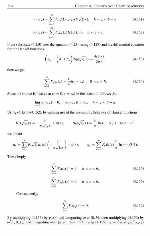
204 Chapter 4. Oceans over Elastic Basements
ur(r, z) =∞∑n=0
Fn√ξnαn(z)H(
√ξnr), h < z < b + h, (4.151)
uz(r, z) =∞∑n=0
Fnβn(z)H(√ξnr), h < z < b. (4.152)
If we substitute (4.150) into the equation (4.23), using (4.128) and the differential equationfor the Hankel functions(
∂rr + 1
r∂r + ξn
)H0(
√ξnr) = 4iδ(r)
2πr, (4.153)
then we get
∞∑n=1
Fngn(z) = i
4δ(z− z0), 0 < z < h. (4.154)
Since the source is located at (r = 0, z = z0) in the ocean, it follows that
limr→0
ur(r, z) = 0, |uz(r, z)| <∞, h < z < b + h.
Using (4.151)–(4.152), by making use of the asymptotic behavior of Hankel functions
H1(√ξnx) = − 2i
π√ξnx
+ o(x), H0(√ξnx) = 2i
πln x +O(1) as x → 0,
we obtain
ur =∞∑n=1
Fn√ξnαn(z)
(− 2i
π√ξnr
)+ o(r), uz =
∞∑n=1
Fnβn(z)2i
πln r +O(1).
These imply
∞∑n=1
Fnαn(z) = 0, h < z < b, (4.155)
∞∑n=1
Fnβn(z) = 0, h < z < b. (4.156)
Consequently,
∞∑n=1
Fnα′n(z) = 0. (4.157)
By multiplying (4.154) by gm(z) and integrating over [0, h], then multiplying (4.156) byω2ρwβm(z) and integrating over [h, b], then multiplying (4.155) by −ω2ρwρ(z)ω
2αm(z)
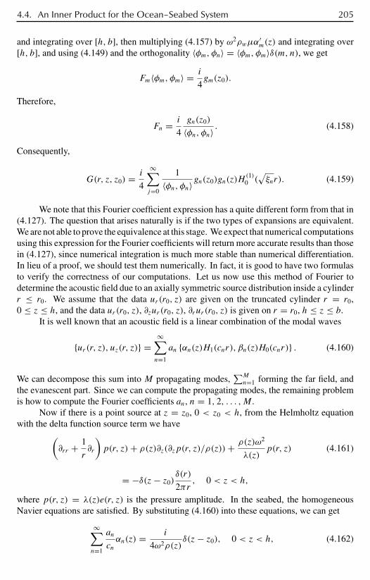
4.4. An Inner Product for the Ocean–Seabed System 205
and integrating over [h, b], then multiplying (4.157) by ω2ρwµα′m(z) and integrating over
[h, b], and using (4.149) and the orthogonality 〈φm, φn〉 = 〈φm, φm〉δ(m, n), we get
Fm〈φm, φm〉 = i
4gm(z0).
Therefore,
Fn = i
4
gn(z0)
〈φn, φn〉 . (4.158)
Consequently,
G(r, z, z0) = i
4
∞∑j=0
1
〈φn, φn〉gn(z0)gn(z)H(1)0 (
√ξnr). (4.159)
We note that this Fourier coefficient expression has a quite different form from that in(4.127). The question that arises naturally is if the two types of expansions are equivalent.We are not able to prove the equivalence at this stage. We expect that numerical computationsusing this expression for the Fourier coefficients will return more accurate results than thosein (4.127), since numerical integration is much more stable than numerical differentiation.In lieu of a proof, we should test them numerically. In fact, it is good to have two formulasto verify the correctness of our computations. Let us now use this method of Fourier todetermine the acoustic field due to an axially symmetric source distribution inside a cylinderr ≤ r0. We assume that the data ur(r0, z) are given on the truncated cylinder r = r0,0 ≤ z ≤ h, and the data ur(r0, z), ∂zur(r0, z), ∂rur(r0, z) is given on r = r0, h ≤ z ≤ b.
It is well known that an acoustic field is a linear combination of the modal waves
ur(r, z), uz(r, z) =∞∑n=1
an αn(z)H1(cnr), βn(z)H0(cnr) . (4.160)
We can decompose this sum into M propagating modes,∑Mn=1 forming the far field, and
the evanescent part. Since we can compute the propagating modes, the remaining problemis how to compute the Fourier coefficients an, n = 1, 2, . . . ,M .
Now if there is a point source at z = z0, 0 < z0 < h, from the Helmholtz equationwith the delta function source term we have(
∂rr + 1
r∂r
)p(r, z)+ ρ(z)∂z(∂zp(r, z)/ρ(z))+ ρ(z)ω2
λ(z)p(r, z) (4.161)
= −δ(z− z0)δ(r)
2πr, 0 < z < h,
where p(r, z) = λ(z)e(r, z) is the pressure amplitude. In the seabed, the homogeneousNavier equations are satisfied. By substituting (4.160) into these equations, we can get
∞∑n=1
an
cnαn(z) = i
4ω2ρ(z)δ(z− z0), 0 < z < h, (4.162)
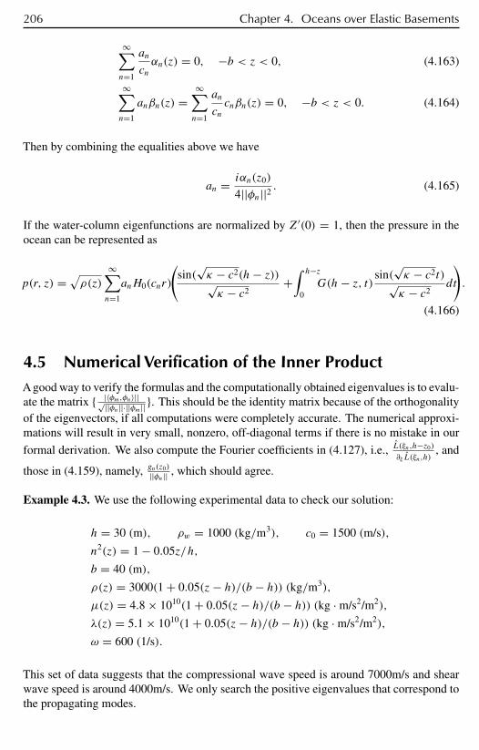
206 Chapter 4. Oceans over Elastic Basements
∞∑n=1
an
cnαn(z) = 0, −b < z < 0, (4.163)
∞∑n=1
anβn(z) =∞∑n=1
an
cncnβn(z) = 0, −b < z < 0. (4.164)
Then by combining the equalities above we have
an = iαn(z0)
4||φn||2 . (4.165)
If the water-column eigenfunctions are normalized by Z′(0) = 1, then the pressure in theocean can be represented as
p(r, z) = √ρ(z)
∞∑n=1
anH0(cnr)
(sin(
√κ − c2(h− z))√κ − c2
+∫ h−z
0G(h− z, t) sin(
√κ − c2t)√κ − c2
dt
).
(4.166)
4.5 Numerical Verification of the Inner ProductA good way to verify the formulas and the computationally obtained eigenvalues is to evalu-ate the matrix |〈φm,φn〉||√||φn||·||φm|| . This should be the identity matrix because of the orthogonalityof the eigenvectors, if all computations were completely accurate. The numerical approxi-mations will result in very small, nonzero, off-diagonal terms if there is no mistake in our
formal derivation. We also compute the Fourier coefficients in (4.127), i.e., L(ξn,h−z0)
∂ξ L(ξn,h), and
those in (4.159), namely, gn(z0)
||φn|| , which should agree.
Example 4.3. We use the following experimental data to check our solution:
h = 30 (m), ρw = 1000 (kg/m3), c0 = 1500 (m/s),
n2(z) = 1 − 0.05z/h,
b = 40 (m),
ρ(z) = 3000(1 + 0.05(z− h)/(b − h)) (kg/m3),
µ(z) = 4.8 × 10¹⁰(1 + 0.05(z− h)/(b − h)) (kg · m/s2/m2),
λ(z) = 5.1 × 10¹⁰(1 + 0.05(z− h)/(b − h)) (kg · m/s2/m2),
ω = 600 (1/s).
This set of data suggests that the compressional wave speed is around 7000m/s and shearwave speed is around 4000m/s. We only search the positive eigenvalues that correspond tothe propagating modes.

4.5. Numerical Verification of the Inner Product 207
Table 4.2. The comparison of Fourier coefficients.
n ξnL(ξn,h)
∂ξ (ξn,h)in (4.127) gn(z0)
T (n,n)in (4.159)
1 2.719182e-02 -1.717591e-02 -1.725774e-022 9.176573e-02 -1.203690e-02 -1.205485e-023 1.353713e-01 7.586275e-03 7.610731e-034 1.569599e-01 2.312212e-03 2.319580e-03
0 5 10 15 20 25 30−10
−5
0
5
10
15
20
25
z
g[n]
(z)
Figure 4.12. Eigenfunc-tions gn(z), n = 1, 2, 3, 4, in theocean.
30 31 32 33 34 35 36 37 38 39 40−8
−6
−4
−2
0
2
4
6
8
10x 10
−10
z
alph
a[n]
(z)
Figure 4.13. Eigenfunc-tions αn(z) in the seabed.
The matrix T (m,n)√|T (m,m)T (n,n)| is as follows:
1.00000 0.00344 0.00288 0.002810.00344 1.00000 0.00160 0.001160.00288 0.00160 1.00000 0.001170.00281 0.00116 0.00117 1.00000
.
Figure 4.15 shows the procedure for searching eigenvalues. We use the combinationof a brute-force search and the bisection method. It turns out that computing ∂ξ L(ξ, h)is very expensive, so we approximate it by central differences. The eigenfunctions gn areplotted in Figure 4.12, αn(z) in Figure 4.13, and βn(z) in Figure 4.14. Finally, in order to seethe effect of interaction of the seabed on the far field, we compare an elastic seabed with thetotally reflecting seabed, using the following data as input: ocean as in Example 4.3; elasticseabed with constant cl = 7000m/s, ct = 4000m/s, and b = 10m; frequency ω = 600 1/s;depth of the source z0 = 15m; range r = 2000m. Figure 4.16 shows the comparisonbetween the case of a totally reflecting seabed and that of an elastic seabed. We can seefrom the far field that the effect of the seabed interaction is significant.
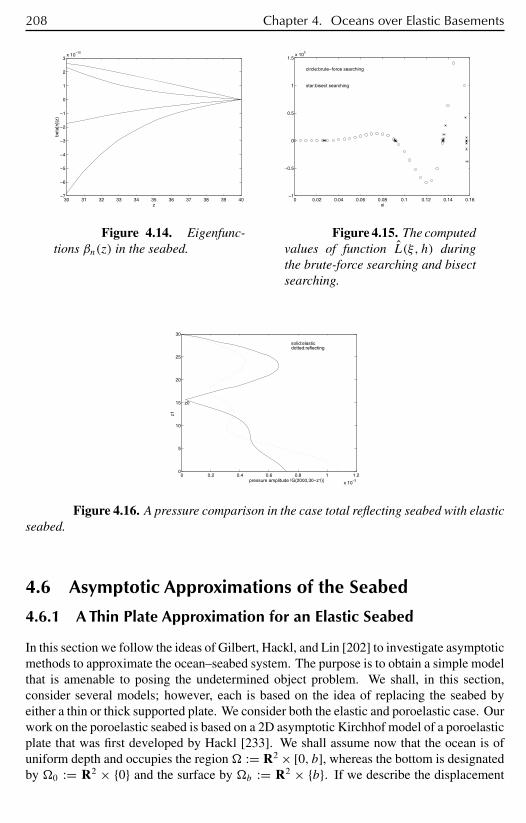
208 Chapter 4. Oceans over Elastic Basements
30 31 32 33 34 35 36 37 38 39 40−7
−6
−5
−4
−3
−2
−1
0
1
2
3x 10
−10
z
beta
[n](
z)
Figure 4.14. Eigenfunc-tions βn(z) in the seabed.
0 0.02 0.04 0.06 0.08 0.1 0.12 0.14 0.16−1
−0.5
0
0.5
1
1.5x 10
5
xi
star:bisect searching
circle:brute−force searching
Figure 4.15. The computedvalues of function L(ξ, h) duringthe brute-force searching and bisectsearching.
0 0.2 0.4 0.6 0.8 1 1.2
x 10−3
0
5
10
15
20
25
30
z1
pressure amplitude !G(2000,30−z1)|
z0
solid:elasticdotted:reflecting
Figure 4.16. A pressure comparison in the case total reflecting seabed with elasticseabed.
4.6 Asymptotic Approximations of the Seabed
4.6.1 A Thin Plate Approximation for an Elastic Seabed
In this section we follow the ideas of Gilbert, Hackl, and Lin [202] to investigate asymptoticmethods to approximate the ocean–seabed system. The purpose is to obtain a simple modelthat is amenable to posing the undetermined object problem. We shall, in this section,consider several models; however, each is based on the idea of replacing the seabed byeither a thin or thick supported plate. We consider both the elastic and poroelastic case. Ourwork on the poroelastic seabed is based on a 2D asymptotic Kirchhof model of a poroelasticplate that was first developed by Hackl [233]. We shall assume now that the ocean is ofuniform depth and occupies the region := R2 × [0, b], whereas the bottom is designatedby 0 := R2 × 0 and the surface by b := R2 × b. If we describe the displacement
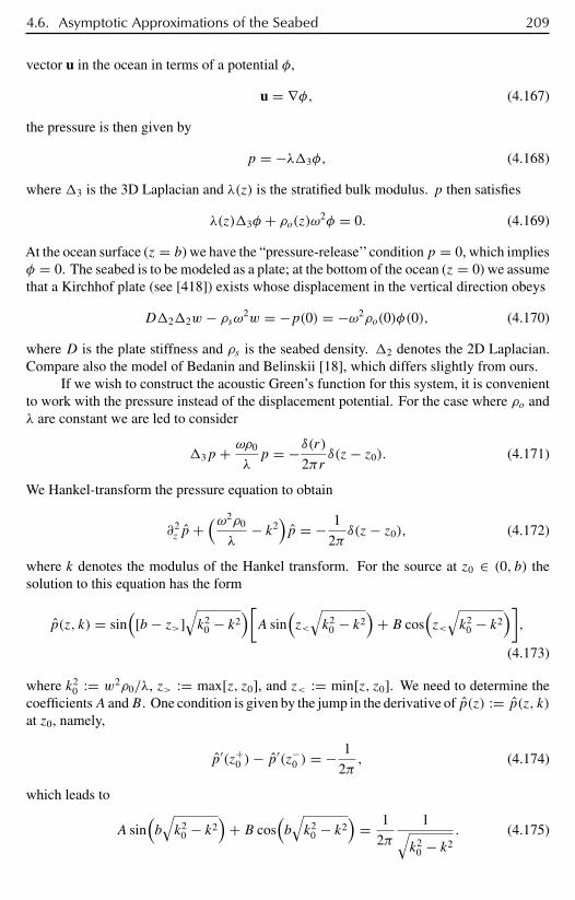
4.6. Asymptotic Approximations of the Seabed 209
vector u in the ocean in terms of a potential φ,
u = ∇φ, (4.167)
the pressure is then given by
p = −λ3φ, (4.168)
where 3 is the 3D Laplacian and λ(z) is the stratified bulk modulus. p then satisfies
λ(z)3φ + ρo(z)ω2φ = 0. (4.169)
At the ocean surface (z = b) we have the “pressure-release’’conditionp = 0, which impliesφ = 0. The seabed is to be modeled as a plate; at the bottom of the ocean (z = 0) we assumethat a Kirchhof plate (see [418]) exists whose displacement in the vertical direction obeys
D22w − ρsω2w = −p(0) = −ω2ρo(0)φ(0), (4.170)
where D is the plate stiffness and ρs is the seabed density. 2 denotes the 2D Laplacian.Compare also the model of Bedanin and Belinskii [18], which differs slightly from ours.
If we wish to construct the acoustic Green’s function for this system, it is convenientto work with the pressure instead of the displacement potential. For the case where ρo andλ are constant we are led to consider
3p + ωρ0
λp = −δ(r)
2πrδ(z− z0). (4.171)
We Hankel-transform the pressure equation to obtain
∂2z p +
(ω2ρ0
λ− k2
)p = − 1
2πδ(z− z0), (4.172)
where k denotes the modulus of the Hankel transform. For the source at z0 ∈ (0, b) thesolution to this equation has the form
p(z, k) = sin([b − z>]
√k2
0 − k2)[A sin
(z<
√k2
0 − k2)
+ B cos(z<
√k2
0 − k2)],
(4.173)
where k20 := w2ρ0/λ, z> := max[z, z0], and z< := min[z, z0]. We need to determine the
coefficientsA andB. One condition is given by the jump in the derivative of p(z) := p(z, k)
at z0, namely,
p′(z+0 )− p′(z−0 ) = − 1
2π, (4.174)
which leads to
A sin(b
√k2
0 − k2)
+ B cos(b
√k2
0 − k2)
= 1
2π
1√k2
0 − k2. (4.175)
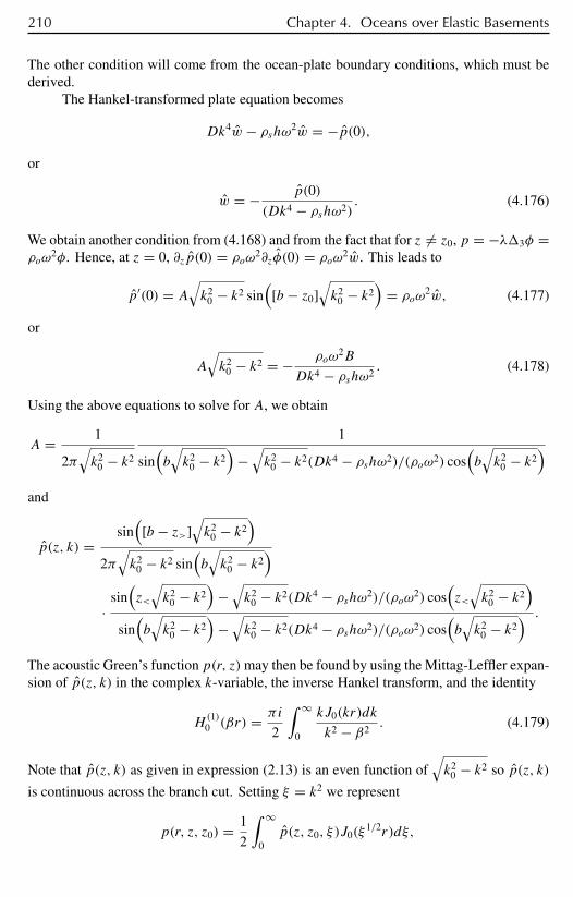
210 Chapter 4. Oceans over Elastic Basements
The other condition will come from the ocean-plate boundary conditions, which must bederived.
The Hankel-transformed plate equation becomes
Dk4w − ρshω2w = −p(0),or
w = − p(0)
(Dk4 − ρshω2). (4.176)
We obtain another condition from (4.168) and from the fact that for z = z0, p = −λ3φ =ρoω
2φ. Hence, at z = 0, ∂zp(0) = ρoω2∂zφ(0) = ρoω
2w. This leads to
p′(0) = A
√k2
0 − k2 sin([b − z0]
√k2
0 − k2)
= ρoω2w, (4.177)
or
A
√k2
0 − k2 = − ρoω2B
Dk4 − ρshω2. (4.178)
Using the above equations to solve for A, we obtain
A = 1
2π√k2
0 − k2
1
sin(b
√k2
0 − k2)
−√k2
0 − k2(Dk4 − ρshω2)/(ρoω2) cos(b
√k2
0 − k2)
and
p(z, k) =sin([b − z>]
√k2
0 − k2)
2π√k2
0 − k2 sin(b
√k2
0 − k2)
·sin(z<
√k2
0 − k2)
−√k2
0 − k2(Dk4 − ρshω2)/(ρoω2) cos
(z<
√k2
0 − k2)
sin(b
√k2
0 − k2)
−√k2
0 − k2(Dk4 − ρshω2)/(ρoω2) cos(b
√k2
0 − k2) .
The acoustic Green’s function p(r, z)may then be found by using the Mittag-Leffler expan-sion of p(z, k) in the complex k-variable, the inverse Hankel transform, and the identity
H(1)0 (βr) = πi
2
∫ ∞
0
kJ0(kr)dk
k2 − β2. (4.179)
Note that p(z, k) as given in expression (2.13) is an even function of√k2
0 − k2 so p(z, k)
is continuous across the branch cut. Setting ξ = k2 we represent
p(r, z, z0) = 1
2
∫ ∞
0p(z, z0, ξ)J0(ξ
1/2r)dξ,
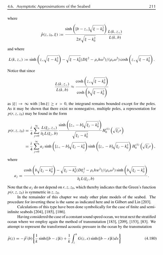
4.6. Asymptotic Approximations of the Seabed 211
where
p(z, z0, ξ) :=sinh
([b − z>]
√ξ − k2
0
)2π√ξ − k2
0
L(k, z<)
L(k, b)
and where
L(k, z<) := sinh
(z<
√ξ − k2
0
)−√ξ − k2
0(Dξ2 − ρshω2)/(ρoω
2) cosh
(z<
√ξ − k2
0
).
Notice that since
L(k, z<)
L(k, b)≈
cosh
(z<
√ξ − k2
0
)cosh
(b
√ξ − k2
0
)as |ξ | → ∞ with | Im ξ | ≥ ε > 0, the integrand remains bounded except for the poles.As it may be shown that there exist no nonnegative, multiple poles, a representation forp(r, z, z0) may be found in the form
p(r, z, z0) = i
4
∞∑j=0
L(ξj , z<)
∂ξL(ξj , b)
sinh
([z> − b]
√ξj − k2
0
)√ξj − k2
0
H(1)0
(√ξj r
)
= i
4
∞∑j=0
aj sinh
([z< − b]
√ξj − k2
0
)sinh
([z> − b]
√ξj − k2
0
)H(1)0
(√ξj r
),
where
aj =cosh
(b
√ξj − k2
0
)−√ξj − k2
0(Dξ2j − ρshw2)/(ρoω
2) sinh
(b
√ξj − k2
0
)∂ξL(ξj , b)
.
Note that the aj do not depend on r, z, z0, which thereby indicates that the Green’s functionp(r, z, z0) is symmetric in z, z0.
In the remainder of this chapter we study other plate models of the seabed. Theprocedure for inverting these is the same as indicated here and in Gilbert and Lin [203].
Calculations of this type have been done symbolically for the case of finite and semi-infinite seabeds [204], [185], [186].
Having considered the case of a constant sound speed ocean, we treat next the stratifiedocean where we employ again the method of transmutation [183], [209], [153], [83]. Weattempt to represent the transformed acoustic pressure in the ocean by the transmutation
p(z) = −p′(b)
1
ksinh([b − z]k)+ 1
k
∫ b
z
G(z, s) sinh([b − s]k)ds
(4.180)
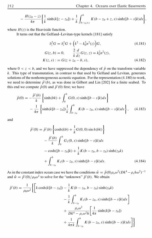
212 Chapter 4. Oceans over Elastic Basements
− H(z0 − z)4π
1
ksinh(k[z− z0])+ 1
k
∫ b
b−z0+zK(b − z0 + z, s) sinh([b − s]k)ds
,
where H(z) is the Heaviside function.It turns out that the Gelfand–Levitan-type kernels [181] satisfy
∂2zG = ∂2
s G+(k2 − k2
0n2(z)
)G, (4.181)
G(z, b) = 0,2
k
d
dzG(z, z) = k2
0n2(z),
K(z, s) : = G(z+ z0 − b, s), (4.182)
where 0 < z < b, and we have suppressed the dependency of p on the transform variablek. This type of transmutation, in contrast to that used by Gelfand and Levitan, generatessolutions of the nonhomogeneous acoustic equation. For the representation (4.180) to work,we need to determine p′(b), as was done in Gilbert and Lin [202] for a finite seabed. Tothis end we compute p(0) and p′(0) first; we have
p(0) = − p′(b)k
sinh(bk)+
∫ b
0G(0, s) sinh([b − s]k)ds
− 1
4π
sinh(k[b − z0])1
k
∫ b
b−z0
K(b − z0, s) sinh([b − s]k)ds, (4.183)
and
p′(0) = p′(b)
cosh(kb)+ 1
kG(0, 0) sin h(bk)
− p′(b)
k
∫ b
0G1(0, s) sinh([b − s]k)ds
− cosh([b − z0]k)+ 1
kK(b − z0, b − z0) sinh(z0k)
+∫ b
b−z0
K1(b − z0, s) sinh([b − s]k)ds. (4.184)
As in the constant index ocean case we have the conditions w = p(0)ρoω2(Dk4 −ρshω2)−1
and w = p′(0)/ρ0ω2 to solve for the “unknown’’ p′(b). We obtain
p′(b) = 1
ρ0ω2
[k cosh(k[b − z0])− 1
kK(b − z0, b − z0) sinh(z0k)
− 1
k
∫ b
b−z0
K1(b − z0, s) sinh([b − s]k)ds]
+ ρoω2
Dk4 − ρsω2h
[1
4πsinh(k[b − z0])
+ 1
4πk
∫ b
b−z0
K(b − z0, s) sinh([b − s]k)ds]
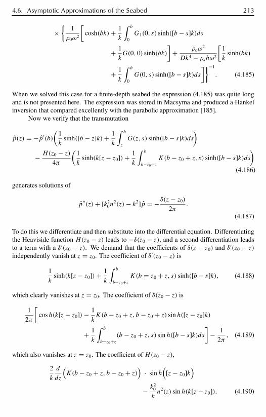
4.6. Asymptotic Approximations of the Seabed 213
×
1
ρ0ω2
[cosh(bk)+ 1
k
∫ b
0G1(0, s) sinh([b − s]k)ds
+ 1
kG(0, 0) sinh(bk)
]+ ρoω
2
Dk4 − ρshω2
[1
ksinh(bk)
+ 1
k
∫ b
0G(0, s) sinh([b − s]k)ds
]−1
. (4.185)
When we solved this case for a finite-depth seabed the expression (4.185) was quite longand is not presented here. The expression was stored in Macsyma and produced a Hankelinversion that compared excellently with the parabolic approximation [185].
Now we verify that the transmutation
p(z) = −p′(b)(
1
ksinh([b − z]k)+ 1
k
∫ b
z
G(z, s) sinh([b − s]k)ds)
− H(z0 − z)4π
(1
ksinh(k[z− z0])+ 1
k
∫ b
b−z0+zK(b − z0 + z, s) sinh([b − s]k)ds
)(4.186)
generates solutions of
p′′(z)+ [k20n
2(z)− k2]p = −δ(z− z0)
2π.
(4.187)
To do this we differentiate and then substitute into the differential equation. Differentiatingthe Heaviside function H(z0 − z) leads to −δ(z0 − z), and a second differentiation leadsto a term with a δ′(z0 − z). We demand that the coefficients of δ(z − z0) and δ′(z0 − z)
independently vanish at z = z0. The coefficient of δ′(z0 − z) is
1
ksinh(k[z− z0])+ 1
k
∫ b
b−z0+zK(b = z0 + z, s) sinh([b − s]k), (4.188)
which clearly vanishes at z = z0. The coefficient of δ(z0 − z) is
1
2π
[cosh(k[z− z0])− 1
kK(b − z0 + z, b − z0 + z) sin h([z− z0]k)
+ 1
k
∫ b
b−z0+z(b − z0 + z, s) sin h([b − s]k)ds
]− 1
2π, (4.189)
which also vanishes at z = z0. The coefficient of H(z0 − z),2
k
d
dz
(K(b − z0 + z, b − z0 + z)
)· sin h
([z− z0]k
)− k2
0
kn2(z) sin h(k[z− z0]), (4.190)
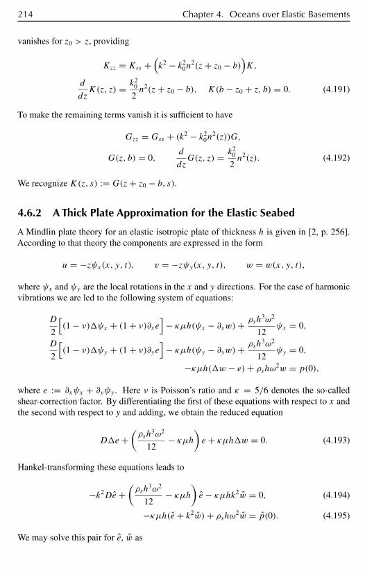
214 Chapter 4. Oceans over Elastic Basements
vanishes for z0 > z, providing
Kzz = Kss +(k2 − k2
0n2(z+ z0 − b)
)K,
d
dzK(z, z) = k2
0
2n2(z+ z0 − b), K(b − z0 + z, b) = 0. (4.191)
To make the remaining terms vanish it is sufficient to have
Gzz = Gss + (k2 − k20n
2(z))G,
G(z, b) = 0,d
dzG(z, z) = k2
0
2n2(z). (4.192)
We recognize K(z, s) := G(z+ z0 − b, s).
4.6.2 A Thick Plate Approximation for the Elastic Seabed
A Mindlin plate theory for an elastic isotropic plate of thickness h is given in [2, p. 256].According to that theory the components are expressed in the form
u = −zψx(x, y, t), v = −zψy(x, y, t), w = w(x, y, t),
where ψx and ψy are the local rotations in the x and y directions. For the case of harmonicvibrations we are led to the following system of equations:
D
2
[(1 − ν)ψx + (1 + ν)∂xe
]− κµh(ψx − ∂xw)+ ρsh
3ω2
12ψx = 0,
D
2
[(1 − ν)ψy + (1 + ν)∂ye
]− κµh(ψy − ∂yw)+ ρsh
3ω2
12ψy = 0,
−κµh(w − e)+ ρshω2w = p(0),
where e := ∂xψx + ∂yψy . Here ν is Poisson’s ratio and κ = 5/6 denotes the so-calledshear-correction factor. By differentiating the first of these equations with respect to x andthe second with respect to y and adding, we obtain the reduced equation
De +(ρsh
3ω2
12− κµh
)e + κµhw = 0. (4.193)
Hankel-transforming these equations leads to
−k2De +(ρsh
3ω2
12− κµh
)e − κµhk2w = 0, (4.194)
−κµh(e + k2w)+ ρshω2w = p(0). (4.195)
We may solve this pair for e, w as

4.6. Asymptotic Approximations of the Seabed 215
e = κµhk2p(0)(ρsh3ω2/12 −Dk2 − κµh
)(ρshω2 − κµhk2
)+ κ2µ2h2k2
, (4.196)
w = (ρsh3ω2/12 −Dk2 − κµh)p(0)(
ρsh3ω2/12 −Dk2 − κµh)(ρshω2 − κµhk2
)+ κ2µ2h2k2
. (4.197)
We choose for the constant index ocean the representation (4.180) for p(z). We now proceedas in the thin plate approximation. Once again we can solve for the coefficients A and B.Substitution in (4.180) yields
p(z, k) =sin([b − z>]
√k2
0 − k2)
2π√k2
0 − k2 sin(b
√k2
0 − k2)
·sin(z<
√k2
0 − k2)
+√k2
0 − k2C(k) cos(z<
√k2
0 − k2)
sin(b
√k2
0 − k2)
+√k2
0 − k2C(k) cos(b
√k2
0 − k2) ,
with
C(k) =(ρsh
3ω2/12 −Dk2 − κµh)(ρshω
2 − κµhk2)
+ κ2µ2h2k2
(ρsh3ω2/12 −Dk2 − κµh)ρoω2. (4.198)
For the stratified ocean we again use the same representation to determine p′(b). To thisend we compute
p′(0) = E1(k)p′(b)+ E2(k), (4.199)
p(0) = E3(k)p′(b)+ E4(k), (4.200)
with
E1(k) := cosh(bk)+ 1
kG(0, 0) sinh(bk)− 1
k
∫ b
0G1(0, s) sinh
([b − s]k
)ds,
E2(k) := − cosh([b − z0]k
)+ 1
kK(b − z0, b − z0) sinh(z0b)
+ 1
k
∫ b
b−z0
K1(b − z0, s) sinh([b − s]k
)ds,
E3(k) := − sinh(bk)−∫ b
0G(0, s) sinh
([z− s]k
)ds,
E4(k) := − 1
4πsinh
(k[z− z0]
)− 1
4πk
∫ b
b−z0
K(b − z0, s) sinh([b − s]k
)ds.
Then we obtain

216 Chapter 4. Oceans over Elastic Basements
p′(b) = −E4(k)− C(k)E2(k)
E3(k)− C(k)E1(k), (4.201)
and we have
e = 1
ρoω2C(k)
κµhk2
ρsh3ω2/12 −Dk2 − κµh(E3(k)p
′(b)+ E4(k)), (4.202)
w = 1
ρoω2C(k)
(E3(k)p
′(b)+ E4(k)). (4.203)
Chapter 5
Shallow Oceans overPoroelastic Seabeds
5.1 IntroductionIn a shallow ocean, sound waves travelling distances of several kilometers will interactrepeatedly with the underlying seabed. Consequently, in developing a mathematical meansfor predicting acoustic pressure in a shallow ocean the manner in which the seabed ismodelled is important. In such computations the seabed typically is treated as a dense fluid,an elastic solid, or a poroelastic medium. As indicated in Vidmar [439], [440] the fluidmodel is appropriate for thick sediment layers, but thin sediment layers, where conversionof energy to shear waves is an important loss mechanism, require a model that supports sheareffects. Examples of the poor predictions made by the fluid model for thin sediment layerscan be found in Hughes et al. [249]. Since thin superficial sediment layers are common inshallow ocean environments, our concern will be a comparison of the solid elastic modelwith the poroelastic model developed by Biot in [36], [38], [40], [39]. This chapter is basedon a series of papers by Buchanan and Gilbert [65], [75], [79], [81] and the paper [84] ofBuchanan, Gilbert, and Xu.
5.2 Elastic Model of a SeabedThe elastic model of a seabed is widely used in ocean acoustics. Hence, before deriv-ing Biot’s model for a porous medium, let us summarize the equations for the elasticmodel. A sediment layer is treated as a viscoelastic slab depending upon the parame-ters ρ, the aggregate density of the layer; λ and µ, the compressional and shear Lamécoefficients; and γp and γs , the compressional and shear attenuation coefficients. Let thevector u(x, y, z, t) = [ux(x, y, z, t), uy(x, y, z, t), uz(x, y, z, t)] track displacement of amaterial point in the seabed. The dilatation e = ∇ · u then measures the relative volu-metric increment due to deformation. The constitutive equations for an isotropic elasticmaterial are
σxx = λe + 2µexx, (5.1)
σyy = λe + 2µeyy,
217
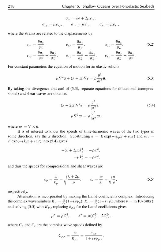
218 Chapter 5. Shallow Oceans over Poroelastic Seabeds
σzz = λe + 2µezz,
σxy = µexy, σxz = µexz, σyz = µeyz,
where the strains are related to the displacements by
exx = ∂ux
∂x, eyy = ∂uy
∂y, ezz = ∂uz
∂z, (5.2)
exy = ∂ux
∂y+ ∂uy
∂x, exz = ∂ux
∂z+ ∂uz
∂x, eyz = ∂uy
∂z+ ∂uz
∂y.
For constant parameters the equation of motion for an elastic solid is
µ∇2u + (λ+ µ)∇e = ρ∂2
∂t2u. (5.3)
By taking the divergence and curl of (5.3), separate equations for dilatational (compres-sional) and shear waves are obtained:
(λ+ 2µ)∇2e = ρ∂2
∂t2e, (5.4)
µ∇2! = ρ∂2
∂t2!,
where! = ∇ × u.It is of interest to know the speeds of time-harmonic waves of the two types in
some direction, say the x direction. Substituting e = E exp(−ikpx + iωt) and !x =F exp(−iksx + iωt) into (5.4) gives
−(λ+ 2µ)k2p = −ρω2,
−µk2s = −ρω2,
and thus the speeds for compressional and shear waves are
cp = ω
kp=√λ+ 2µ
ρ, cs = ω
ks=õ
ρ, (5.5)
respectively.Attenuation is incorporated by making the Lamé coefficients complex. Introducing
the complex wavenumbersKp = ωcp(1+iνγp),Ks = ω
cs(1+iνγs), where ν = ln 10/(40π),
and solving (5.5) with Kp,s replacing kp,s for the Lamé coefficients gives
µ∗ = ρC2s , λ∗ = ρ(C2
p − 2C2s ),
where Cp and Cs are the complex wave speeds defined by
Cp,s = ω
Kp,s= cp,s
1 + iνγp,s .
5.3. The Poroelastic Model of a Seabed 219
The normalization factor ν is inserted so that the loss in decibels over one wavelength2π/k is
L = −20 log
∣∣∣∣exp
(iK
(2π
k
))∣∣∣∣ = −20 log exp(−2πνγ ) = γ.
The units for γ are said to be “decibels per wavelength.’’ In ocean acoustic literatureattenuation is often written in the form
= Af, (5.6)
where is measured in dB/m, f is the frequency measured in kHz, and thus the constantK is in dB/m/kHz. In terms of γ the loss per meter is
= γ
(2πc/ω)= 1000γ
cf,
which gives the formula for converting between the coefficients A and γ .
5.3 The Poroelastic Model of a SeabedThe most commonly used model for a poroelastic medium is that developed by Biot in [35],[36], [38], [40], [39]. In sections 5.3.1 and 5.3.2 we sketch the derivation of Biot’s model.In section 5.3.3 we discuss the calculation of the parameters in the model from the set ofinput parameters introduced by Stoll [400]. In section 5.3.4 sets of Biot–Stoll parameterstaken from the literature are given and the difficulties in determining these parameters arediscussed.
5.3.1 Constitutive Equations for an Isotropic Porous Medium
The Biot model treats the medium as an elastic frame with interstitial pore fluid. Twodisplacement vectors u(x, y, z, t) = [ux(x, y, z, t), uy(x, y, z, t), uz(x, y, z, t)] andU(x, y, z, t) = [Ux(x, y, z, t), Uy(x, y, z, t), Uz(x, y, z, t)] track the motion of the frameand fluid, respectively, while the divergences e = ∇ · u and ε = ∇ · U give the frameand fluid dilatations. We shall treat only the case of an isotropic frame. In this case theframe has six components of stress, σxx, σyy, σzz, σxy, σxz, σyz. The corresponding strainswill be denoted by exx, eyy, ezz, exy, exz, eyz. The fluid stress in the pore space is given byσ(x, y, z, t) = −βpf , where pf is the pressure of the pore fluid and the parameter β isthe fraction of fluid area per unit cross section. Biot makes the assumption of statisticalisotropy, that is, that β is the same for all cross sections. Thus β is equal to the porosity ofthe medium (volume of the pore space per unit volume).
In an isotropic medium the strain energy will be a function
W = W(I1, I2, I3, ε),
where the Ij are the three elastic invariants (see Love [295])
I1 = exx + eyy + ezz = e,
220 Chapter 5. Shallow Oceans over Poroelastic Seabeds
I2 = eyyezz + exxezz + exxeyy − 1
4(e2yz + e2
xz + e2xy),
I3 = exxeyyezz + 1
4(eyzexzexy − exxe2
yz − eyye2xz − ezze2
xy).
For small amplitude vibrations we can neglect powers of the displacements above the firstorder and obtain linear constitutive equations. This corresponds to a strain energy functionthat is purely quadratic in the strains and hence it will be a linear combination of the fourquadratic terms e2, I2, eε, and ε2:
W = P
2e2 − 2µI2 +Qeε + R
2ε2.
The components of stress are related to the strain energy function by
σxx = ∂W
∂exx, . . . , σyz = ∂W
∂eyz, σ = ∂W
∂ε.
This gives the constitutive equations
σxx = Pe − 2µ(eyy + ezz
)+Qε,σyy = Pe − 2µ (exx + ezz)+Qε,σzz = Pe − 2µ
(exx + eyy
)+Qε,σxy = µexy, σxz = µexz, σyz = µeyz,
σ = Qe + Rε.
Since exx + eyy + ezz = e the equations can be put in the form
σxx = λe + 2µexx +Qε, (5.7)
σyy = λe + 2µeyy +Qε,σzz = λe + 2µezz +Qε,σxy = µexy, σxz = µexz, σyz = µeyz,
σ = Qe + Rε
with λ = P − 2µ. The symbols assigned to the parameters λ and µ are due to theirformal analogy to the Lamé coefficients in the constitutive equations (5.1) of an elasticsolid. Indeed, the tangential stress equations (5.7)4 suggest that µ is the Lamé coefficient ofshear for the frame. However, as we shall see, λ is not the frame compressional coefficient.
5.3.2 Dynamical Equations for a Porous Medium
In [36] Biot adopted the following form for the kinetic energy of the system
T = 1
2
[ρ11
(.u
2x + .
u2y + .
u2z
)+ 2ρ12
(.ux
.
Ux + .uy
.
Uyx + .uz
.
Uz
)
5.3. The Poroelastic Model of a Seabed 221
+ ρ22
(.
U2
x + .
U2
y + .
U2
z
)], (5.8)
where.ux = ∂ux
∂t, . . . . Thus ρ11 and ρ22 are effective mass density parameters of the frame
and fluid, respectively, and ρ12 is a mass coupling parameter for the frame–fluid interaction.A Rayleigh dissipation function
D = 1
2b
[(.ux − .
Ux
)2 +(.uy − .
Uy
)2 +(.uz −
.
Uz
)2]
is introduced to account for energy loss due to the motion of the fluid relative to that of theframe. The lagrangian equations of motion are
∂σxx
∂x+ ∂σxy
∂y+ ∂σxz
∂z= d
dt
(∂T
∂.ux
)+ ∂D
∂.ux,
∂σxy
∂x+ ∂σyy
∂y+ ∂σyz
∂z= d
dt
(∂T
∂.uy
)+ ∂D
∂.uy,
∂σxz
∂x+ ∂σyz
∂y+ ∂σzz
∂z= d
dt
(∂T
∂.uz
)+ ∂D
∂.uz,
∂σ
∂x= d
dt
(∂T
∂.
Ux
)+ ∂D
∂.
Ux
,
∂σ
∂y= d
dt
(∂T
∂.
Uy
)+ ∂D
∂.
Uy
,
∂σ
∂z= d
dt
(∂T
∂.
Uz
)+ ∂D
∂.
Uz
.
Substituting the constitutive equations (5.7) and the strain-displacement relations (5.2) givesthe equations of motion
∂
∂x
(λe + 2µ
∂ux
∂x+Qε
)+ ∂
∂y
(µ
(∂ux
∂y+ ∂uy
∂x
))(5.9)
+ ∂
∂z
(µ
(∂ux
∂z+ ∂uz
∂x
))= ∂2
∂t2(ρ11ux + ρ12Ux)+ b ∂
∂t(ux − Ux) ,
∂
∂y
(λe + 2µ
∂uy
∂y+Qε
)+ ∂
∂x
(µ
(∂uy
∂x+ ∂ux
∂y
))+ ∂
∂z
(µ
(∂uy
∂z+ ∂uz
∂y
))= ∂2
∂t2
(ρ11uy + ρ12Uy
)+ b ∂∂t
(uy − Uy
),
∂
∂z
(λe + 2µ
∂uz
∂z+Qε
)+ ∂
∂y
(µ
(∂uz
∂y+ ∂uy
∂z
))
222 Chapter 5. Shallow Oceans over Poroelastic Seabeds
+ ∂
∂x
(µ
(∂ux
∂z+ ∂uz
∂x
))= ∂2
∂t2(ρ11uz + ρ12Uz)+ b ∂
∂t(uz − Uz) ,
∂
∂x(Qe + Rε) = ∂2
∂t2(ρ12ux + ρ22Ux)− b ∂
∂t(ux − Ux),
∂
∂y(Qe + Rε) = ∂2
∂t2(ρ12uy + ρ22Uy)− b ∂
∂t(uy − Uy),
∂
∂z(Qe + Rε) = ∂2
∂t2(ρ12uz + ρ22Uz)− b ∂
∂t(uz − Uz).
In the case where all parameters are constant, we have, upon expressing the cross partialderivatives in terms of the derivatives of the dilatations, the considerably simpler vectorequations
µ∇2u + ∇[(λ+ µ)e +Qε] = ∂2
∂t2(ρ11u + ρ12U)+ b ∂
∂t(u − U), (5.10)
∇[Qe + Rε] = ∂2
∂t2(ρ12u + ρ22U)− b ∂
∂t(u − U).
The form of the dissipation parameter b is complicated. In [38] Biot gave the formula
b = F(a√ωρf /η
)β2η
k(5.11)
when the medium is undergoing time-harmonic oscillations of angular frequency ω. Hereρf is the density of the pore fluid, η is the viscosity of the fluid, k is the Darcy permeabilityof the medium, and a is referred to as the pore size parameter. The function F is given by
F(ζ ) = 1
4
ζT (ζ )
1 − 2T (ζ )/iζ,
where T is defined in terms of Kelvin functions
T (ζ ) = ber′(ζ )+ ibei′(ζ )ber(ζ )+ ibei(ζ )
.
Figure 5.1 shows the graphs of |F | and its real and imaginary parts. At low frequenciesthe flow of the fluid is of Poiseuille type; i.e., inertial effects are inconsequential relative toviscous effects. The purpose of the function F is to correct for the increased influence ofinertial terms at higher frequencies. Biot estimates the range of validity of the Poiseuilleregime to be 0 ≤ ζ ≤ √
3.
5.3.3 Calculation of the Coefficients in the Biot Model
The equations of motion (5.10) depend upon the parameters λ, µ, R, Q, ρ11, ρ12, ρ22, andb, which need to be calculated from measured and estimated seabed parameters. We seek
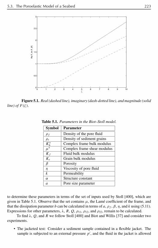
5.3. The Poroelastic Model of a Seabed 223
0 1 2 3 4 5 6 7 8 9 100
0.5
1
1.5
2
2.5
3
ζ
Re
F, I
m F
, |F
|
Figure 5.1. Real (dashed line), imaginary (dash-dotted line), and magnitude (solidline) of F(ζ ).
Table 5.1. Parameters in the Biot–Stoll model.
Symbol Parameterρf Density of the pore fluidρr Density of sediment grainsK∗b Complex frame bulk modulus
µ∗ Complex frame shear modulusKf Fluid bulk modulusKr Grain bulk modulusβ Porosityη Viscosity of pore fluidk Permeabilityα Structure constanta Pore size parameter
to determine these parameters in terms of the set of inputs used by Stoll [400], which aregiven in Table 5.1. Observe that the set contains µ, the Lamé coefficient of the frame, andthat the dissipation parameter b can be calculated in terms of a, ρf , β, η, and k using (5.11).Expressions for other parameters, λ, R,Q, ρ11, ρ12, and ρ22, remain to be calculated.
To find λ,Q, and R we follow Stoll [400] and Biot and Willis [37] and consider twoexperiments.
• The jacketed test: Consider a sediment sample contained in a flexible jacket. Thesample is subjected to an external pressure p′, and the fluid in the jacket is allowed
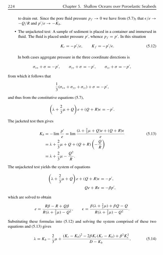
224 Chapter 5. Shallow Oceans over Poroelastic Seabeds
to drain out. Since the pore fluid pressure pf → 0 we have from (5.7)5 that ε/e →−Q/R and p′/e → −Kb.
• The unjacketed test: A sample of sediment is placed in a container and immersed influid. The fluid is placed under pressure p′, whence pf = p′. In this situation
Kr = −p′/e, Kf = −p′/ε. (5.12)
In both cases aggregate pressure in the three coordinate directions is
σxx + σ = −p′, σyy + σ = −p′, σzz + σ = −p′,
from which it follows that
1
3(σxx + σyy + σzz)+ σ = −p′,
and thus from the constitutive equations (5.7),(λ+ 2
3µ+Q
)e + (Q+ R)ε = −p′.
The jacketed test then gives
Kb = − limp′
e= lim
(λ+ 23µ+Q)e + (Q+ R)ε
e(5.13)
= λ+ 2
3µ+Q+ (Q+ R)
(−QR
)= λ+ 2
3µ− Q2
R.
The unjacketed test yields the system of equations(λ+ 2
3µ+Q
)e + (Q+ R)ε = −p′,
Qe + Rε = −βp′,
which are solved to obtain
e = Rβ − R +QβR(λ+ 2
3µ)−Q2, ε = β(λ+ 2
3µ)+ βQ−QR(λ+ 2
3µ)−Q2.
Substituting these formulas into (5.12) and solving the system comprised of these twoequations and (5.13) gives
λ = Kb − 2
3µ+ (Kr −Kb)2 − 2βKr(Kr −Kb)+ β2K2
r
D −Kb , (5.14)
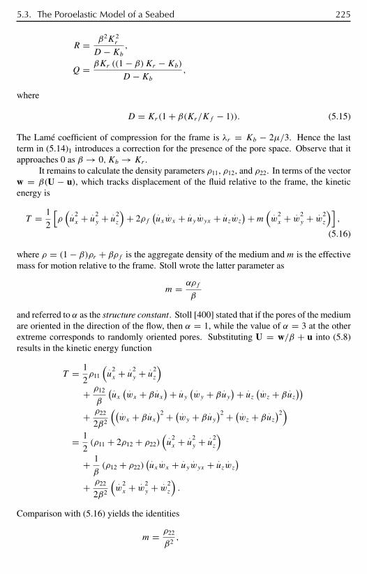
5.3. The Poroelastic Model of a Seabed 225
R = β2K2r
D −Kb ,
Q = βKr ((1 − β)Kr −Kb)D −Kb ,
where
D = Kr(1 + β(Kr/Kf − 1)). (5.15)
The Lamé coefficient of compression for the frame is λr = Kb − 2µ/3. Hence the lastterm in (5.14)1 introduces a correction for the presence of the pore space. Observe that itapproaches 0 as β → 0,Kb → Kr .
It remains to calculate the density parameters ρ11, ρ12, and ρ22. In terms of the vectorw = β(U − u), which tracks displacement of the fluid relative to the frame, the kineticenergy is
T = 1
2
[ρ(.u
2x + .
u2y + .
u2z
)+ 2ρf
( .ux
.wx + .
uy.wyx + .
uz.wz)+m
(.w
2x + .
w2y + .
w2z
)],
(5.16)
where ρ = (1 − β)ρr + βρf is the aggregate density of the medium and m is the effectivemass for motion relative to the frame. Stoll wrote the latter parameter as
m = αρf
β
and referred to α as the structure constant. Stoll [400] stated that if the pores of the mediumare oriented in the direction of the flow, then α = 1, while the value of α = 3 at the otherextreme corresponds to randomly oriented pores. Substituting U = w/β + u into (5.8)results in the kinetic energy function
T = 1
2ρ11
(.u
2x + .
u2y + .
u2z
)+ ρ12
β
( .ux( .wx + β .ux
)+ .uy( .wy + β .uy
)+ .uz( .wz + β .uz
))+ ρ22
2β2
(( .wx + β .ux
)2 + ( .wy + β .uy
)2 + ( .wz + β .uz
)2)
= 1
2(ρ11 + 2ρ12 + ρ22)
(.u
2x + .
u2y + .
u2z
)+ 1
β(ρ12 + ρ22)
( .ux
.wx + .
uy.wyx + .
uz.wz)
+ ρ22
2β2
(.w
2x + .
w2y + .
w2z
).
Comparison with (5.16) yields the identities
m = ρ22
β2,

226 Chapter 5. Shallow Oceans over Poroelastic Seabeds
Table 5.2. Grain and frame parameters for the Biot–Stoll model for five sediments.
Sediment ρr Kr β k α a
FS 2670 4.0 × 10¹⁰ 0.43 3.12 × 10⁻¹⁴ 1.25 1.20 × 10⁻⁶
CS 2710 5.6 × 10¹⁰ 0.38 7.5 × 10⁻¹¹ 1.25 6.28 × 10⁻⁵
CSFG 2680 4.0 × 10¹⁰ 0.30 2.58 × 10⁻¹⁰ 1.25 1.31 × 10⁻⁴
SS 2670 3.8 × 10¹⁰ 0.65 6.33 × 10⁻¹⁵ 3.0 4.25 × 10⁻⁷
SC 2680 3.5 × 10¹⁰ 0.68 5.2 × 10⁻¹⁴ 3.0 1.24 × 10⁻⁶
ρf = 1
β(ρ12 + ρ22) ,
ρ = ρ11 + 2ρ12 + ρ22,
from which it follows that
ρ11 = (1 − β)ρr − β(ρf −mβ),ρ12 = β(ρf −mβ),ρ22 = mβ2.
In deriving the Biot model the frame was regarded as purely elastic. A realistic modelmust allow for attenuation due to intergranular friction. Biot [40], Stoll [400], and Stolland Bryan [406] argued by appeal to viscoelastic models that this can be accomplishedadequately by introducing frequency-independent imaginary components to the moduliKband µ to obtain complex moduli that we will denote byK∗
b and µ∗. However, in [405] Stollsuggested that for fine, silty sediments a second loss mechanism, the “squeeze film’’ effect,which is frequency dependent, may be significant. Under what is termed the correspondenceprinciple by Biot, the complex versions of the remaining moduli λ∗, R∗, and Q∗ can beobtained by substituting K∗
b and µ∗ into the relations (5.14).
5.3.4 Experimental Determination of the Biot–Stoll Inputs
In order to evaluate the Biot model we shall examine its predictions for the acoustic fieldfor five different sediments encompassing the range of types that may be expected in ashallow ocean environment. The test suite, the parameters for which are shown in Table5.2, consists of a coarse to medium sand (CS) sediment off of Daytona Beach, Florida and asilty sand (SS) sediment off of Corpus Christi, Texas, for which most of the parameters weretaken from Beebe, McDaniel, and Rubano [26], and a coarse sand and fine gravel (CSFG)sediment, a fine sand (FS) sediment, and a silty clay (SC) sediment located at three differentsites in the Gulf of La Spezia, Italy, with the parameters mostly taken from Holland andBrunson [245].
The parameters of Table 5.1 fall into three categories: pore fluid parameters ρf , Kf ,and η; grain parameters ρr andKr ; and frame parametersKb, µ, β, k, α, and a. To illustratethe considerations involved in determining the Biot–Stoll parameters we shall examine thetechniques used by the two sets of authors cited above. Further discussion and alternatives
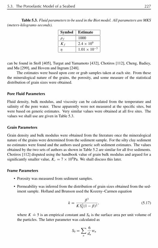
5.3. The Poroelastic Model of a Seabed 227
Table 5.3. Fluid parameters to be used in the Biot model. All parameters are MKS(meters-kilograms-seconds).
Symbol Estimateρf 1000
Kf 2.4 × 10⁹
η 1.01 × 10⁻³
can be found in Stoll [405], Turgut and Yamamoto [432], Chotiros [112], Cheng, Badiey,and Mu [299], and Hovem and Ingram [248].
The estimates were based upon core or grab samples taken at each site. From thesethe mineralogical nature of the grains, the porosity, and some measure of the statisticaldistribution of grain sizes were obtained.
Pore Fluid Parameters
Fluid density, bulk modulus, and viscosity can be calculated from the temperature andsalinity of the pore water. These apparently were not measured at the specific sites, butwere based on generic estimates. Very similar values were obtained at all five sites. Thevalues we shall use are given in Table 5.3.
Grain Parameters
Grain density and bulk modulus were obtained from the literature once the mineralogicalnature of the grains were determined from the sediment sample. For the silty clay sedimentno estimates were found and the authors used generic soft sediment estimates. The valuesobtained by the two sets of authors as shown in Table 5.2 are similar for all five sediments.Chotiros [112] disputed using the handbook value of grain bulk modulus and argued for asignificantly smaller value, Kr = 7 × 10⁹Pa. We shall discuss this later.
Frame Parameters
• Porosity was measured from sediment samples.
• Permeability was inferred from the distribution of grain sizes obtained from the sed-iment sample. Holland and Brunson used the Kozeny–Carmen equation
k = β3
KS20(1 − β)2 , (5.17)
where K.= 5 is an empirical constant and S0 is the surface area per unit volume of
the particles. The latter parameter was calculated as
S0 =∑n
6
dnwn

228 Chapter 5. Shallow Oceans over Poroelastic Seabeds
from a discrete set (dn, wn) of grain sizes dn and proportions wn of total volumeobtained by sorting the sample. Beebe et al. used a different empirical relation due toKrumbien and Monk, which depends upon the mean Mφ and standard deviation σφof grain sizes in φ units
k = 7.6d2e−1.31σφ × 10−6,
where d = 2−Mφ mm is the mean grain diameter.
• Shear and bulk moduli were calculated from generic parameters for the type of sed-iment. Holland and Brunson calculated the frame shear modulus from the empiricalformula of Hardin and Richart for sands and clays,
µ = 1230(2.97 − ε)2
1 + ε√σ0, (5.18)
in pounds per square inch. Here
ε = β
1 − βis the voids ratio, and the mean effective stress due to over burden pressure is
σ0 = 1 + 2K0
3
∫ z
0g(1 − β(z))(ρr − ρf )dz, (5.19)
where z is the depth in the seabed,K0 is the coefficient of earth pressure at rest, whichis typically taken to be 0.5, and g is the acceleration due to gravity. The complexmoduli were then calculated from
µ∗ = (1 + iµ/π)µ, (5.20)
K∗b = 2(1 + Rp)
3(1 − 2Rp)µ(1 + iKb/π),
whereKb andµ are the log decrements for compressional and shear vibrations andRp is the Poisson ratio. Since Holland and Brunson were interested in wave velocityand attenuation near the sediment surface, they used a depth of z = 0.1m in (5.19).
An alternative to (5.18) due to Bryan and Stoll [64], [405] is to assume a func-tional form for the shear modulus
µ1 = paa exp(bε)(σ0/pa)n, (5.21)
where pa is the atmospheric pressure. Based on statistical regressions on laboratoryresults, Stoll arrived at the values a = 2526, b = −1.504, and n = 0.448. As fieldtests tend to lead to somewhat higher values for the shear modulus than laboratoryresults, Stoll suggested an empirical modification µ = FF · µ1, where FF = 2.
Beebe et al. used the formulas
E∗ = (1 − β)ρrV 2E(1 + iE/π), (5.22)

5.4. Solution of the Time-Harmonic Biot Equations 229
G∗ = (1 − β)ρrV 2S (1 + iS/π),
K∗b = − E∗G∗
3(E∗ − 3G∗)
of Stoll and Bryan [406]. HereVE andVS are the uniaxial velocities for compressionaland shear vibrations, respectively, andE andS are the log decrements for the twotypes of vibrations. Thus both sets of authors use frequency-independent choices forthe complex moduli, which means as mentioned earlier that they take into accountintergranular friction, but not the squeeze film effect.
• The pore size parameter is generally agreed to be proportional to√k. It was calculated
by Holland and Brunson from an empirical relation of Hovem and Ingram [248]
a = 2
√Kk
β. (5.23)
Beebe et al., following Stoll, used the empirical relation a.= √
k/0.26.
• Both sets of authors follow Stoll in assigning a value of α = 1.25 for “clean’’ sandsand α = 3 for silty sediments. This parameter seems to be of little influence whenconventional estimates of the grain bulk modulus Kr such as those in Table 5.2 areused, but is more significant if the lower value of this modulus suggested by Chotirosis employed.
Table 5.2 gives estimates for some of the grain and frame parameters of the Biot–Stoll model for the five sediments. The values shown were taken from the articles citedabove with the exception that the pore size parameter was calculated from (5.23) for all fivesediments. The calculation of the moduli K∗
b and µ∗ will be discussed in section 5.4.2.
5.4 Solution of the Time-Harmonic Biot Equations
5.4.1 Simplification of the Equations
For a medium that is assumed to oscillate harmonically in time, we have u(x, y, z, t) =u(x, y, z)eiωt , U(x, y, z, t) = U(x, y, z)eiωt , . . . . Substituting these representations intothe constant parameter equations (5.10) gives
µ∇2u + ∇[(λ+ µ)e +Qε] + p11u + p12U = 0, (5.24)
∇[Qe + Rε] + p12u + p22U = 0,
where
p11 := ω2ρ11 − iωb, p12 := ω2ρ12 + iωb, p22 := ω2ρ22 − iωb. (5.25)
Taking the divergence and curl of both equations in (5.24) yields the system
∇2((λ+ 2µ)e +Qε)+ p11e + p12ε = 0, (5.26)
230 Chapter 5. Shallow Oceans over Poroelastic Seabeds
∇2(Qe + Rε)+ p12e + p22ε = 0,
µ∇2! + p11! + p12 = 0,
p12! + p22 = 0,
where! := ∇ × u and := ∇ × U.In the first two equations of (5.26) we make the change of dependent variables
τ := (λ+ 2µ)e +Qε, σ := Qe + Rε, (5.27)
the inverse transformation for which is
e = a11τ − a12σ, ε = −a12τ + a22σ, (5.28)
where
a11 := R/d, a12 := Q/d, a22 := (λ+ 2µ)/d
with
d := R(λ+ 2µ)−Q2.
Note that for the transformation given by (5.27) to be nonsingular it must be the case thatd = 0,∞. From (5.14)
d = (3Kb + 4µ)Kbβ2
3 (D −Kb) ,
whereD is given by (5.15). SinceKr > Kb,Kf implies thatD > Kr > Kb, it follows that0 < d <∞.
Thus we have from (5.26)1,2
∇2τ + B11τ + B12σ = 0, (5.29)
∇2σ + B21τ + B22σ = 0,
where
B11 := a11p11 − a12p12, B12 := −a12p11 + a22p12,
B21 := a11p12 − a12p22, B22 := −a12p12 + a22p22.
From (5.24)2 the fluid displacement vector is
U = − 1
p22(∇σ + p12u) . (5.30)
Substituting this into (5.24)1 gives a partial differential equation for the frame displacementvector
∇2u + A31∇τ + A32∇σ + B33u = 0, (5.31)

5.4. Solution of the Time-Harmonic Biot Equations 231
where
A31 := 1 − µa11
µ, A32 := a12 − p12
µp22, B33 := p11p22 − p2
12
µp22.
Also the third and fourth equations of (5.26) imply that shear waves in the frame satisfy
∇2! + B33! = 0. (5.32)
In section 5.3.4 we saw that the moduli are expected to vary with depth due to overbur-den pressure. Thus it is of interest to examine the equations that result when the four moduliλ, µ, R, and Q depend upon depth and all other parameters are assumed constant. Uponwriting the cross partials in (5.9) in terms of the dilatations, eliminating the components ofU, and introducing the coordinate change (5.27) we obtain the system
∇2
τ
σ
uz
+ A ∂∂z
τ
σ
uz
+ B τ
σ
uz
= 0, (5.33)
where the elements of the matrices A and B are given by
A11 = −2µ′(z)µ(z)
, A12 = 2p11µ
′(z)p22µ(z)
, A13 = 2µ′′(z)− 4µ′(z)2
µ(z), (5.34)
A21 = A22 = A33 = 0,
A31 = −R(z)d(z)
+ 1
µ(z), A32 = −Q(z)
3
d(z)2+ 2
µ(z)R(z)Q(z)
d(z)2+ λ(z)R(z)Q(z)
d(z)2,
A33 = 2µ′(z)µ(z)
,
B11 = −Q(z)p12
d(z)+ 4
µ′(z)2
µ(z)d(z)− 2
µ′′(z)R(z)d(z)
+ p11R(z)
d(z), (5.35)
B12 = −4µ′(z)2Q(z)µ(z)d(z)
+ 2p12µ(z)
d(z)+ 2
µ′′(z)Q(z)d(z)
+ p12λ(z)
d(z)− p11Q(z)
d(z),
B13 = −2p11µ
′(z)µ(z)
+ 2p2
12µ′(z)
p22µ(z),
B21 = p12R(z)
d(z)− p22Q(z)
d(z),
B22 = 2p22µ(z)
d(z)+ p22λ(z)
d(z)− p12Q(z)
d(z),
B23 = 0,
B31 = λ(z)R(z)R′(z)d(z)2
− R′(z)d(z)
− 2R(z)Q(z)Q′(z)
d(z)2+ R(z)2λ′(z)
d(z)2
+ 2R(z)2µ′(z)d(z)2
− 2R(z)µ′(z)µ(z)d(z)
+ 2µ(z)R(z)R′(z)
d(z)2,
232 Chapter 5. Shallow Oceans over Poroelastic Seabeds
B32 = −λ(z)Q(z)R′(z)
d(z)2− 2
µ(z)Q(z)R′(z)d(z)2
− 2Q(z)3µ′(z)µ(z)d(z)2
− Q′(z)d(z)
+ 2λ(z)R(z)Q′(z)
d(z)2+ 2
R(z)Q(z)µ′(z)d(z)2
+ 4µ(z)R(z)Q′(z)
d(z)2
− R(z)Q(z)λ′(z)d(z)2
+ 2λ(z)R(z)Q(z)µ′(z)
µ(z)d(z)2,
B33 = p11
µ(z)− p2
12
p22µ(z).
As indicated by (5.29), the equations for τ and σ are independent of the components of uin the case of constant seabed parameters. Observe that this remains true in the quasi-staticcase, in which the moduli λ,µ,R, andQ are allowed to vary with depth, but their derivativesare set to zero.
5.4.2 Speeds of Compressional and Shear Waves
Proceeding in the manner of section 5.2, we can ascertain the speed of propagation andattenuation of dilatational and shear waves in the x direction for the constant coefficientequations. Because the time-harmonic variation has already been incorporated into thecoefficients of equations (5.29) we seek solutions of the form τ(x) = c1e
−ikpx and σ(x) =c2e
−ikpx . To represent a physical (spatially decaying) solution the imaginary part of thecomplex wavenumber kp must be positive. Substituting these forms into (5.29) and requiringthe constants c1 and c2 to be arbitrary gives the condition(
B11 − k2p
) (B22 − k2
p
)− B12B21 = 0,
from which two possible physical wavenumbers
kp± =√B11 + B22 ±√
(B11 − B22)2 + 4B12B21
2(5.36)
are obtained. The branch cut for the outer square root is taken to lie along the positive realaxis so that Im kp± ≥ 0. The sign of Re kp± may be either positive or negative. If we write
kp± = ω
cp±(sgn(Re kp±)+ iνγp±),
where ν = ln 10/(40π) and the attenuation coefficients γp± are measured in decibels perwavelength, then the compressional wave speeds and attenuation coefficients for the twowaves are given by
cp± = ω∣∣Re kp±∣∣ , γp± = Im kp±
ν∣∣Re kp±
∣∣ . (5.37)
A similar analysis of equation (5.32) gives
ks = √B33, (5.38)
5.4. Solution of the Time-Harmonic Biot Equations 233
Table 5.4. Bulk moduli of five sediments.
Sediment Stoll–Bryan Bryan–Stoll (z = 1m) Chotiros
FS 4.8 × 10⁷ + 6.7 × 10⁵i 3.9 × 10⁷ + 1.9 × 10⁶i 4.0 × 10⁹ + 1.9 × 10⁸i
CS 5.3 × 10⁷ + 7.4 × 10⁵i 5.1 × 10⁷ + 2.4 × 10⁶i 7.9 × 10⁹ + 2.5 × 10⁸i
CSFG 5.9 × 10⁷ + 8.2 × 10⁵i 7.1 × 10⁷ + 3.4 × 10⁶i 7.6 × 10⁹ + 3.6 × 10⁸i
SS 2.9 × 10⁷ + 1.3 × 10⁶i 6.0 × 10⁶ + 6.6 × 10⁵i
SC 2.6 × 10⁷ + 1.2 × 10⁶i 3.9 × 10⁶ + 6.2 × 10⁵i
Table 5.5. Shear moduli of five sediments.
Sediment Stoll–Bryan Bryan–Stoll (z = 1m)
FS 6.7 × 10⁷ + 4.3 × 10⁶i 2.4 × 10⁷ + 1.1 × 10⁶i
CS 7.4 × 10⁷ + 4.7 × 10⁶i 3.1 × 10⁷ + 1.8 × 10⁶i
CSFG 8.3 × 10⁷ + 5.3 × 10⁶i 4.3 × 10⁷ + 2.0 × 10⁶i
SS 2.9 × 10⁷ + 1.3 × 10⁶i 3.6 × 10⁶ + 5.7 × 10⁵i
SC 3.4 × 10⁷ + 7.2 × 10⁶i 2.3 × 10⁶ + 3.7 × 10⁵i
cs = ω
|Re ks | , γs = Im ksν |Re ks |
for the speed and attenuation of shear waves through the frame. The compressional wavescorresponding to the wavenumbers kp+ and kp− are sometimes referred to as Type I andType II compressional waves. As we shall see, Type I waves correspond in magnitude tothe compressional waves of the elastic model. Type II waves, which are slower and morestrongly attenuated, do not occur in the elastic model.
In section 5.3.4 two approaches to estimating the complex moduli K∗b and µ∗ were
described. One possibility is to use the Stoll–Bryan formulas (5.22). When using theseformulas we follow [26] in taking the rod velocity to be VE = 300m/s, the shear velocityto be VS = 210m/s, and the log decrements to be E = 0.45 and S = 0.6 for the twosilty sediments and E = 0.15 and S = 0.2 for the other three sand sediments. Theprecise values of VE and VS are not important as the values of the moduli are insensitiveto them in the range around the stated values. Another way to calculate the moduli is touse formula (5.18) or (5.21) in conjunction with (5.20). In formula (5.20) we will use aPoisson ratio of Rp = 0.25, and following Stoll and Kan [407] we will use log decrementsof Kb = µ = 0.15 for the three sand sediments and Kb = µ = 0.5 for the two siltysediments. For unconsolidated sediments the moduli are not very sensitive to the precisechoice of Rp unless it is very near the theoretical upper limit of 0.5. It should be noted,however, that there is not a consensus on the values of the log decrement, with some authorssuch as Turgut and Yamamoto [432] and, later, Stoll in [405] using lower values of Kband µ in the 0.05–0.1 range. Tables 5.4 and 5.5 give the computed complex bulk andshear moduli computed according to the Stoll–Bryan formula (5.22) and the Bryan–Stollformula (5.21) at depth of 1m into the sediment for each of the sediments of Table 5.2. Alsoshown in Table 5.4 are the substantially higher values of the bulk modulus when computed
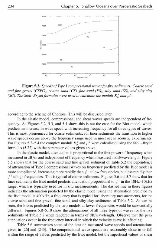
234 Chapter 5. Shallow Oceans over Poroelastic Seabeds
101
102
103
104
105
106
1400
1500
1600
1700
1800
1900
2000
Spe
ed (
m/s
)
Frequency (Hz)
CSFG
CS
FS
SS
SC
Figure 5.2. Speeds of Type I compressional waves for five sediments. Coarse sandand fine gravel (CSFG), coarse sand (CS), fine sand (FS), silty sand (SS), and silty clay(SC). The Stoll–Bryan formulas were used to calculate the moduli K∗
b and µ∗.
according to the scheme of Chotiros. This will be discussed later.In the elastic model, compressional and shear waves speeds are independent of fre-
quency. As Figures 5.2, 5.3, and 5.4 show, this is not the case for the Biot model, whichpredicts an increase in wave speed with increasing frequency for all three types of waves.This is most pronounced for coarse sediments; for finer sediments the transition to higherwave speeds occurs above the frequency range used in most ocean acoustic experiments.For Figures 5.2–5.4 the complex moduli K∗
b and µ∗ were calculated using the Stoll–Bryanformulas (5.22) with the parameter values given above.
In the elastic model, attenuation is proportional to the first power of frequency whenmeasured in dB/m and independent of frequency when measured in dB/wavelength. Figure5.5 shows that for the coarse sand and fine gravel sediment of Table 5.2 the dependenceof attenuation of Type I compressional waves on frequency predicted by the Biot model ismore complicated, increasing more rapidly than f 1 at low frequencies, but less rapidly thanf 1 at high frequencies. This is typical of coarse sediments. Figures 5.6 and 5.7 show that forfiner sediments the Biot model predicts attenuation proportional to f 1 in the 10Hz–10kHzrange, which is typically used for in situ measurements. The dashed line in these figuresindicates the attenuation predicted by the elastic model using the attenuation predicted bythe Biot model at 400kHz, a frequency that is typical for laboratory measurements, for thecoarse sand and fine gravel, fine sand, and silty clay sediments of Table 5.2. As can beseen, the losses predicted by the two models at lower frequencies would be substantiallydifferent. Figures 5.8–5.10 show the attenuations of all three types of waves for the fivesediments of Table 5.2 when rendered in terms of dB/wavelength. Observe that the peakattenuations occur in the frequency interval in which the velocity curve is inflecting.
Table 5.6 summarizes some of the data on measured wave speeds and attenuationsgiven in [26] and [245]. The compressional wave speeds are reasonably close to or fallwithin the range of values predicted by the Biot model, but the superficial values of shear
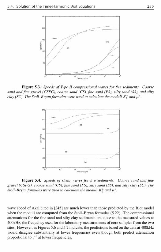
5.4. Solution of the Time-Harmonic Biot Equations 235
101
102
103
104
105
106
0
50
100
150
200
250
Spe
ed (
m/s
)
Frequency (Hz)
CSFG
CS
FS
SC
SS
Figure 5.3. Speeds of Type II compressional waves for five sediments. Coarsesand and fine gravel (CSFG), coarse sand (CS), fine sand (FS), silty sand (SS), and siltyclay (SC). The Stoll–Bryan formulas were used to calculate the moduli K∗
b and µ∗.
101
102
103
104
105
106
150
160
170
180
190
200
210
Spe
ed (
m/s
)
Frequency (Hz)
CSFG
CS
FS
SS
SC
Figure 5.4. Speeds of shear waves for five sediments. Coarse sand and finegravel (CSFG), coarse sand (CS), fine sand (FS), silty sand (SS), and silty clay (SC). TheStoll–Bryan formulas were used to calculate the moduli K∗
b and µ∗.
wave speed of Akal cited in [245] are much lower than those predicted by the Biot modelwhen the moduli are computed from the Stoll–Bryan formulas (5.22). The compressionalattenuations for the fine sand and silty clay sediments are close to the measured values at400kHz, the frequency used for the laboratory measurements of core samples from the twosites. However, as Figures 5.6 and 5.7 indicate, the predictions based on the data at 400kHzwould disagree substantially at lower frequencies even though both predict attenuationproportional to f 1 at lower frequencies.
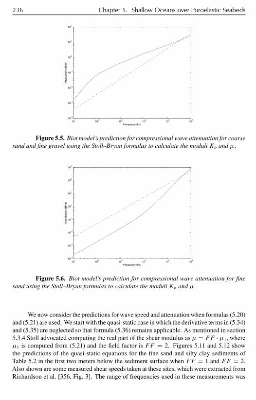
236 Chapter 5. Shallow Oceans over Poroelastic Seabeds
101
102
103
104
105
106
10−4
10−3
10−2
10−1
100
101
102
Atte
nuat
ion
(dB
/m)
Frequency (Hz)
Figure 5.5. Biot model’s prediction for compressional wave attenuation for coarsesand and fine gravel using the Stoll–Bryan formulas to calculate the moduli Kb and µ.
101
102
103
104
105
106
10−4
10−3
10−2
10−1
100
101
102
103
Atte
nuat
ion
(dB
/m)
Frequency (Hz)
Figure 5.6. Biot model’s prediction for compressional wave attenuation for finesand using the Stoll–Bryan formulas to calculate the moduli Kb and µ.
We now consider the predictions for wave speed and attenuation when formulas (5.20)and (5.21) are used. We start with the quasi-static case in which the derivative terms in (5.34)and (5.35) are neglected so that formula (5.36) remains applicable. As mentioned in section5.3.4 Stoll advocated computing the real part of the shear modulus as µ = FF · µ1, whereµ1 is computed from (5.21) and the field factor is FF = 2. Figures 5.11 and 5.12 showthe predictions of the quasi-static equations for the fine sand and silty clay sediments ofTable 5.2 in the first two meters below the sediment surface when FF = 1 and FF = 2.Also shown are some measured shear speeds taken at these sites, which were extracted fromRichardson et al. [356, Fig. 3]. The range of frequencies used in these measurements was

5.4. Solution of the Time-Harmonic Biot Equations 237
101
102
103
104
105
106
10−4
10−3
10−2
10−1
100
101
102
103
Atte
nuat
ion
(dB
/m)
Frequency (Hz)
Figure 5.7. Biot model’s prediction for compressional wave attenuation for siltyclay using the Stoll–Bryan formulas to calculate the moduli Kb and µ.
101
102
103
104
105
106
0
0.2
0.4
0.6
0.8
1
1.2
1.4
Atte
nuat
ion
(dB
/λ)
Frequency (Hz)
CSFG CS
FS
SC
SS
Figure 5.8. Biot model’s prediction for compressional wave attenuation for coarsesand and fine gravel using the Stoll–Bryan formulas to calculate the moduli K∗
b and µ∗.
200–2000Hz, but the Biot model predictions for shear speed vary only slightly over thisrange. As can be seen, the choice FF = 1 better fits the measurements. Hence we shallsimply use equation (5.21) to compute the real part of the shear modulus and disregard thefield factor.
Figures 5.13 and 5.14 show the predictions at frequency 320Hz for the speed of TypeI compressional and shear waves for the five sediments of Table 5.2 as functions of depthwhen the real part of the shear modulus was computed using (5.20) and (5.21).
Figure 5.15 shows that the Stoll–Bryan formula (5.22) and the Bryan–Stoll formula(5.21) at a depth of 1m make very similar predictions for the speed of Type I compressional
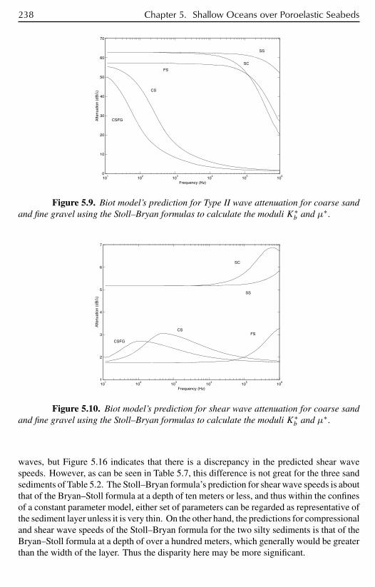
238 Chapter 5. Shallow Oceans over Poroelastic Seabeds
101
102
103
104
105
106
0
10
20
30
40
50
60
70
Atte
nuat
ion
(dB
/λ)
Frequency (Hz)
CSFG
CS
FS
SS
SC
Figure 5.9. Biot model’s prediction for Type II wave attenuation for coarse sandand fine gravel using the Stoll–Bryan formulas to calculate the moduli K∗
b and µ∗.
101
102
103
104
105
106
1
2
3
4
5
6
7
Atte
nuat
ion
(dB
/λ)
Frequency (Hz)
SC
SS
FS CS
CSFG
Figure 5.10. Biot model’s prediction for shear wave attenuation for coarse sandand fine gravel using the Stoll–Bryan formulas to calculate the moduli K∗
b and µ∗.
waves, but Figure 5.16 indicates that there is a discrepancy in the predicted shear wavespeeds. However, as can be seen in Table 5.7, this difference is not great for the three sandsediments of Table 5.2. The Stoll–Bryan formula’s prediction for shear wave speeds is aboutthat of the Bryan–Stoll formula at a depth of ten meters or less, and thus within the confinesof a constant parameter model, either set of parameters can be regarded as representative ofthe sediment layer unless it is very thin. On the other hand, the predictions for compressionaland shear wave speeds of the Stoll–Bryan formula for the two silty sediments is that of theBryan–Stoll formula at a depth of over a hundred meters, which generally would be greaterthan the width of the layer. Thus the disparity here may be more significant.
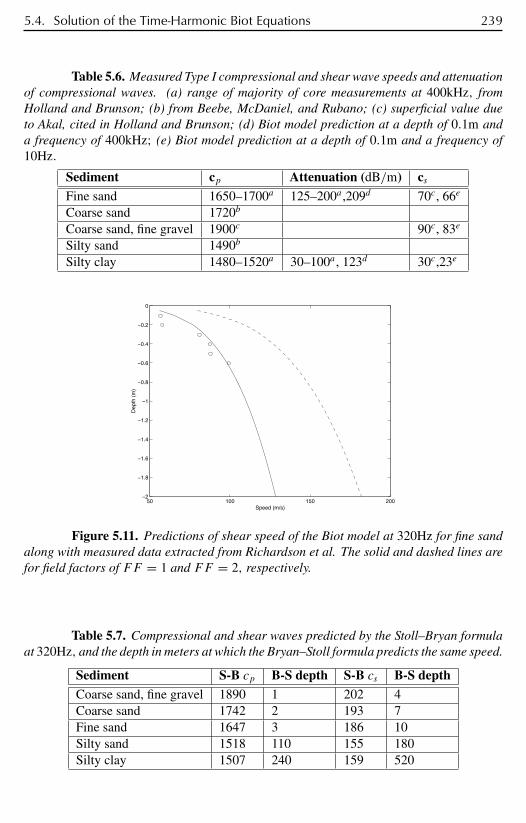
5.4. Solution of the Time-Harmonic Biot Equations 239
Table 5.6. Measured Type I compressional and shear wave speeds and attenuationof compressional waves. (a) range of majority of core measurements at 400kHz, fromHolland and Brunson; (b) from Beebe, McDaniel, and Rubano; (c) superficial value dueto Akal, cited in Holland and Brunson; (d) Biot model prediction at a depth of 0.1m anda frequency of 400kHz; (e) Biot model prediction at a depth of 0.1m and a frequency of10Hz.
Sediment cp Attenuation (dB/m) csFine sand 1650–1700a 125–200a ,209d 70c, 66e
Coarse sand 1720b
Coarse sand, fine gravel 1900c 90c, 83e
Silty sand 1490b
Silty clay 1480–1520a 30–100a , 123d 30c,23e
50 100 150 200−2
−1.8
−1.6
−1.4
−1.2
−1
−0.8
−0.6
−0.4
−0.2
0
Speed (m/s)
Dep
th (
m)
Figure 5.11. Predictions of shear speed of the Biot model at 320Hz for fine sandalong with measured data extracted from Richardson et al. The solid and dashed lines arefor field factors of FF = 1 and FF = 2, respectively.
Table 5.7. Compressional and shear waves predicted by the Stoll–Bryan formulaat 320Hz, and the depth in meters at which the Bryan–Stoll formula predicts the same speed.
Sediment S-B cp B-S depth S-B cs B-S depthCoarse sand, fine gravel 1890 1 202 4Coarse sand 1742 2 193 7Fine sand 1647 3 186 10Silty sand 1518 110 155 180Silty clay 1507 240 159 520
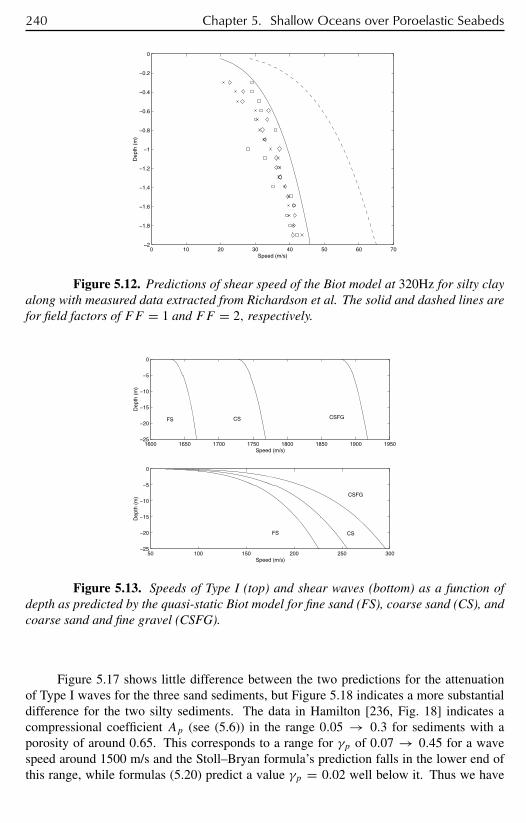
240 Chapter 5. Shallow Oceans over Poroelastic Seabeds
0 10 20 30 40 50 60 70−2
−1.8
−1.6
−1.4
−1.2
−1
−0.8
−0.6
−0.4
−0.2
0
Speed (m/s)
Dep
th (
m)
Figure 5.12. Predictions of shear speed of the Biot model at 320Hz for silty clayalong with measured data extracted from Richardson et al. The solid and dashed lines arefor field factors of FF = 1 and FF = 2, respectively.
1600 1650 1700 1750 1800 1850 1900 1950−25
−20
−15
−10
−5
0
Speed (m/s)
Dep
th (
m)
50 100 150 200 250 300−25
−20
−15
−10
−5
0
Speed (m/s)
Dep
th (
m)
FS CS CSFG
FS CS
CSFG
Figure 5.13. Speeds of Type I (top) and shear waves (bottom) as a function ofdepth as predicted by the quasi-static Biot model for fine sand (FS), coarse sand (CS), andcoarse sand and fine gravel (CSFG).
Figure 5.17 shows little difference between the two predictions for the attenuationof Type I waves for the three sand sediments, but Figure 5.18 indicates a more substantialdifference for the two silty sediments. The data in Hamilton [236, Fig. 18] indicates acompressional coefficient Ap (see (5.6)) in the range 0.05 → 0.3 for sediments with aporosity of around 0.65. This corresponds to a range for γp of 0.07 → 0.45 for a wavespeed around 1500 m/s and the Stoll–Bryan formula’s prediction falls in the lower end ofthis range, while formulas (5.20) predict a value γp = 0.02 well below it. Thus we have

5.4. Solution of the Time-Harmonic Biot Equations 241
1490 1492 1494 1496 1498 1500 1502 1504 1506 1508 1510−25
−20
−15
−10
−5
0
Speed (m/s)
Dep
th (
m)
20 30 40 50 60 70 80 90 100−25
−20
−15
−10
−5
0
Speed (m/s)
Dep
th (
m)
SC SS
SC
SS
Figure 5.14. Speeds of Type I (top) and shear waves (bottom) as a function ofdepth at 320Hz as predicted by the quasi-static Biot model for silty sand (SS) and silty clay(SC).
101
102
103
104
105
106
1400
1500
1600
1700
1800
1900
2000
Spe
ed (
m/s
)
Frequency (Hz)
CSFG
CS
FS
SS
SC
Figure 5.15. Type I compressional wave speeds as predicted by the Stoll–Bryanformula (solid line) and the Bryan–Stoll formula (dashed line) at a depth of 1m below thesediment surface for coarse sand and fine gravel (CSFG), coarse sand (CS), fine sand (FS),silty sand (SS), and silty clay (SC).
the dilemma that the Bryan–Stoll formula makes better predictions for compressional andshear wave speeds for silty sediments, whereas the Stoll–Bryan formula’s predictions forcompressional wave attenuation seem more in accord with the literature.
There is other evidence to support the Biot model’s predictions. For Type I compres-sional waves a frequency dependence conforming reasonably with the Biot model predic-tions has been confirmed both in laboratory measurement for a porous structure composed

242 Chapter 5. Shallow Oceans over Poroelastic Seabeds
101
102
103
104
105
106
20
40
60
80
100
120
140
160
180
200
220
Spe
ed (
m/s
)
Frequency (Hz)
CSFG CS FS
SS SC
Figure 5.16. Shear wave speeds as predicted by the Stoll–Bryan formula (solidline) and the Bryan–Stoll formula (dashed line) at a depth of 1m below the sediment surfacefor coarse sand and fine gravel (CSFG), coarse sand (CS), fine sand (FS), silty sand (SS),and silty clay (SC).
101
102
103
104
105
106
0
0.5
1
1.5
Atte
nuat
ion
(dB
/λ)
Frequency (Hz)
CSFG
CS
FS
Figure 5.17. Type I compresional wave attenuation as predicted by the Stoll–Bryanformula (solid line) and the Bryan–Stoll formula (dash-dotted line) at a depth of 1m belowthe sediment surface for coarse sand and fine gravel (CSFG), coarse sand (CS), and finesand (FS).
of glass beads (Hovem and Ingram [248]) and in situ (Turgut and Yamamoto [432]). Thelatter authors also adduce evidence for dispersion of compressional attenuation with respectto frequency. The laboratory measurements of attenuation of shear waves given in Brunsonand Johnson [63] are also in accord with the Biot model’s predictions. On the other hand,in his 1980 survey article [236] Hamilton found that the evidence from in situ studies at
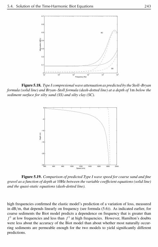
5.4. Solution of the Time-Harmonic Biot Equations 243
101
102
103
104
105
106
0
0.1
0.2
0.3
0.4
0.5
0.6
0.7
Atte
nuat
ion
(dB
/λ)
Frequency (Hz)
SC
SS
Figure 5.18. Type I compresional wave attenuation as predicted by the Stoll–Bryanformula (solid line) and Bryan–Stoll formula (dash-dotted line) at a depth of 1m below thesediment surface for silty sand (SS) and silty clay (SC).
400 600 800 1000 1200 1400 1600 1800 2000−25
−20
−15
−10
−5
0
Speed (m/s)
Dep
th (
m)
Figure 5.19. Comparison of predicted Type I wave speed for coarse sand and finegravel as a function of depth at 10Hz between the variable coefficient equations (solid line)and the quasi-static equations (dash-dotted line).
high frequencies confirmed the elastic model’s prediction of a variation of loss, measuredin dB/m, that depends linearly on frequency (see formula (5.6)). As indicated earlier, forcoarse sediments the Biot model predicts a dependence on frequency that is greater thanf 1 at low frequencies and less than f 1 at high frequencies. However, Hamilton’s doubtswere less about the accuracy of the Biot model than about whether most naturally occur-ring sediments are permeable enough for the two models to yield significantly differentpredictions.
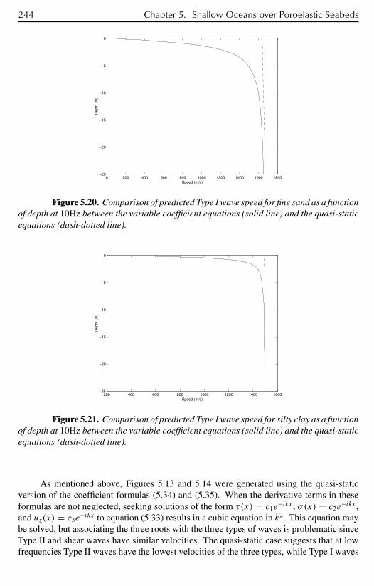
244 Chapter 5. Shallow Oceans over Poroelastic Seabeds
0 200 400 600 800 1000 1200 1400 1600 1800−25
−20
−15
−10
−5
0
Speed (m/s)
Dep
th (
m)
Figure 5.20. Comparison of predicted Type I wave speed for fine sand as a functionof depth at 10Hz between the variable coefficient equations (solid line) and the quasi-staticequations (dash-dotted line).
200 400 600 800 1000 1200 1400 1600−25
−20
−15
−10
−5
0
Speed (m/s)
Dep
th (
m)
Figure 5.21. Comparison of predicted Type I wave speed for silty clay as a functionof depth at 10Hz between the variable coefficient equations (solid line) and the quasi-staticequations (dash-dotted line).
As mentioned above, Figures 5.13 and 5.14 were generated using the quasi-staticversion of the coefficient formulas (5.34) and (5.35). When the derivative terms in theseformulas are not neglected, seeking solutions of the form τ(x) = c1e
−ikx , σ(x) = c2e−ikx ,
and uz(x) = c3e−ikx to equation (5.33) results in a cubic equation in k2. This equation may
be solved, but associating the three roots with the three types of waves is problematic sinceType II and shear waves have similar velocities. The quasi-static case suggests that at lowfrequencies Type II waves have the lowest velocities of the three types, while Type I waves

5.4. Solution of the Time-Harmonic Biot Equations 245
50 100 150 200 250 300−25
−20
−15
−10
−5
0
Speed (m/s)
Dep
th (
m)
Figure 5.22. Comparison of predicted shear wave speed for coarse sand and finegravel as a function of depth at 10Hz between the variable coefficient equations (solid line)and the quasi-static equations (dash-dotted line).
have the highest speeds. Based upon this ansatz, Figures 5.19–5.21 compare the predictionsfor Type I waves as a function of depth at a frequency of 10Hz for the coarse sand and finegravel, fine sand, and silty clay sediments. As can be seen, the variable coefficient formulaspredict very low speeds for Type I waves near the sediment surface with the disparity beinggreater for coarser sediments. On the other hand, Figure 5.22 shows that the predictionsfor shear speed as a function of depth differs little between the quasi-static and the variablecoefficient cases for coarse sand and fine gravel. This is also the case for the other twosediments. Figures 5.23, 5.24 and 5.25 show that at a depth of 1m below the sedimentsurface, the predictions for the speed of Type I waves are in disagreement below 200Hz,while the predictions for Type II and shear wave speeds are in agreement down to about10Hz. We know of no experimental data that confirms the low velocities of Type I wavespredicted by the variable coefficient model, however, most measurements encountered inthe literature that are associated with a specific frequency are at a frequency of a kilohertzor higher. Moreover, Burridge and Keller [91], using the mathematical technique of two-scale homogenization, were able to derive the Biot equations from the microstructure inthe case of constant seabed parameters. However, they found that the variable coefficientequations differed from the Biot equations. Thus there are also theoretical grounds to doubtthe predictions of the variable coefficient model.
Observe from Figures 5.26 and 5.27 that Type II waves are highly attenuated withrespect to range and thus cannot be detected at distances far from the source. Stoll [401]estimated the energy loss due to conversion to Type II waves at the ocean–sediment interfaceto be around 1% at frequencies in the kilohertz range, but smaller at lower frequencies. Thehigh attenuation of Type II waves makes them inherently difficult to detect, however Plona[343] cites possible evidence for their existence. Also, Chotiros has attempted to categorizewaves that have been detected experimentally near the sediment surface at short source-to-receiver distances and shallow grazing angles with speeds in the 1000–1300m/s range as
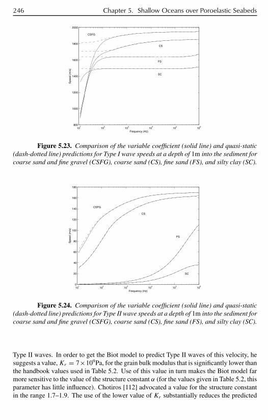
246 Chapter 5. Shallow Oceans over Poroelastic Seabeds
101
102
103
104
105
106
800
1000
1200
1400
1600
1800
2000
Frequency (Hz)
Spe
ed (
m/s
)
CSFG
CS
FS
SC
Figure 5.23. Comparison of the variable coefficient (solid line) and quasi-static(dash-dotted line) predictions for Type I wave speeds at a depth of 1m into the sediment forcoarse sand and fine gravel (CSFG), coarse sand (CS), fine sand (FS), and silty clay (SC).
101
102
103
104
105
106
0
20
40
60
80
100
120
140
160
180
Frequency (Hz)
Spe
ed (
m/s
)
CSFG
CS
FS
SC
Figure 5.24. Comparison of the variable coefficient (solid line) and quasi-static(dash-dotted line) predictions for Type II wave speeds at a depth of 1m into the sediment forcoarse sand and fine gravel (CSFG), coarse sand (CS), fine sand (FS), and silty clay (SC).
Type II waves. In order to get the Biot model to predict Type II waves of this velocity, hesuggests a value,Kr = 7×10⁹Pa, for the grain bulk modulus that is significantly lower thanthe handbook values used in Table 5.2. Use of this value in turn makes the Biot model farmore sensitive to the value of the structure constant α (for the values given in Table 5.2, thisparameter has little influence). Chotiros [112] advocated a value for the structure constantin the range 1.7–1.9. The use of the lower value of Kr substantially reduces the predicted
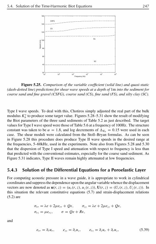
5.4. Solution of the Time-Harmonic Biot Equations 247
101
102
103
104
105
106
20
40
60
80
100
120
140
160
Frequency (Hz)
Spe
ed (
m/s
)
CSFG
CS
FS
SC
Figure 5.25. Comparison of the variable coefficient (solid line) and quasi-static(dash-dotted line) predictions for shear wave speeds at a depth of 1m into the sediment forcoarse sand and fine gravel (CSFG), coarse sand (CS), fine sand (FS), and silty clay (SC).
Type I wave speeds. To deal with this, Chotiros simply adjusted the real part of the bulkmodulusK∗
b to produce some target value. Figures 5.28–5.31 show the result of modifyingthe Biot parameters of the three sand sediments of Table 5.2 as just described. The targetvalues for Type I wave speed were those of Table 5.6 at a frequency of 100Hz. The structureconstant was taken to be α = 1.8, and log decrements of Kb = 0.15 were used in eachcase. The shear moduli were calculated from the Stoll–Bryan formulas. As can be seenin Figure 5.28 this procedure does produce Type II wave speeds in the desired range atthe frequencies, 5–60kHz, used in the experiments. Note also from Figures 5.28 and 5.30that the dispersion of Type I speed and attenuation with respect to frequency is less thanthat predicted with the conventional estimates, especially for the coarse sand sediment. AsFigure 5.31 indicates, Type II waves remain highly attenuated at low frequencies.
5.4.3 Solution of the Differential Equations for a Poroelastic Layer
For computing acoustic pressure in a wave guide, it is appropriate to work in cylindricalcoordinates and suppress the dependence upon the angular variable whence the displacementvectors are now denoted as u(r, z) = (ur(r, z), uz(r, z)),U(r, z) = (Ur(r, z), Uz(r, z)). Inthis situation the relevant constitutive equations (5.7) and strain-displacement relations(5.2) are
σrr = λe + 2µerr +Qε, σzz = λe + 2µezz +Qε,σrz = µerz, σ = Qe + Rε,
and
err = ∂rur , ezz = ∂zuz, erz = ∂zur + ∂ruz, (5.39)
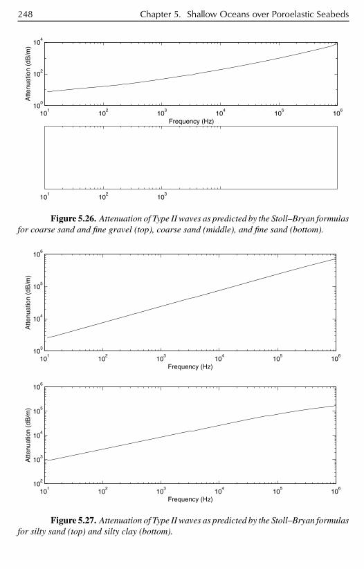
248 Chapter 5. Shallow Oceans over Poroelastic Seabeds
101
102
103
104
105
106
100
102
104
Atte
nuat
ion
(dB
/m)
Frequency (Hz)
101
102
103
Figure 5.26. Attenuation of Type II waves as predicted by the Stoll–Bryan formulasfor coarse sand and fine gravel (top), coarse sand (middle), and fine sand (bottom).
101
102
103
104
105
106
103
104
105
106
Atte
nuat
ion
(dB
/m)
Frequency (Hz)
101
102
103
104
105
106
102
103
104
105
106
Atte
nuat
ion
(dB
/m)
Frequency (Hz)
Figure 5.27. Attenuation of Type II waves as predicted by the Stoll–Bryan formulasfor silty sand (top) and silty clay (bottom).
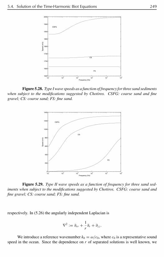
5.4. Solution of the Time-Harmonic Biot Equations 249
101
102
103
104
105
106
1600
1650
1700
1750
1800
1850
1900
1950
2000
Spe
ed (
m/s
)
Frequency (Hz)
CSFG
CS
FS
Figure 5.28. Type I wave speeds as a function of frequency for three sand sedimentswhen subject to the modifications suggested by Chotiros. CSFG: coarse sand and finegravel; CS: coarse sand; FS: fine sand.
101
102
103
104
105
106
0
200
400
600
800
1000
1200
1400
Spe
ed (
m/s
)
Frequency (Hz)
CSFG
CS
FS
Figure 5.29. Type II wave speeds as a function of frequency for three sand sed-iments when subject to the modifications suggested by Chotiros. CSFG: coarse sand andfine gravel; CS: coarse sand; FS: fine sand.
respectively. In (5.26) the angularly independent Laplacian is
∇2 := ∂rr + 1
r∂r + ∂zz.
We introduce a reference wavenumber k0 = ω/c0, where c0 is a representative soundspeed in the ocean. Since the dependence on r of separated solutions is well known, we

250 Chapter 5. Shallow Oceans over Poroelastic Seabeds
101
102
103
104
105
106
0
0.5
1
1.5
2
2.5
3
Atte
nuat
ion
(dB
/λ)
Frequency (Hz)
CSFG
CS
FS
Figure 5.30. Attenuation of Type I waves as a function of frequency for three sandsediments when subject to the modifications suggested by Chotiros. CSFG: coarse sandand fine gravel; CS: coarse sand; FS: fine sand.
101
102
103
104
105
106
0
10
20
30
40
50
60
Atte
nuat
ion
(dB
/λ)
Frequency (Hz)
FS
CS
CSFG
Figure 5.31. Attenuation of Type II waves as a function of frequency for three sandsediments when subject to the modifications suggested by Chotiros. CSFG: coarse sandand fine gravel; CS: coarse sand; FS: fine sand.
seek solutions of the form
τ(r, z) = τ(z)H(1)0 (k0
√κr), σ (r, z) = σ(z)H
(1)0 (k0
√κr), (5.40)
uz(r, z) = uz(z)H(1)0 (k0
√κr), Uz(r, z) = Uz(z)H
(1)0 (k0
√κr),
ur(r, z) = ur(z)H(1)1 (k0
√κr), Ur(r, z) = Ur(z)H
(1)1 (k0
√κr),
whereH(1)j , j = 0, 1, are outgoing Hankel functions and Im(κ) ≥ 0 is required for solutions

5.4. Solution of the Time-Harmonic Biot Equations 251
to approach zero as r → ∞. The presence of the Hankel functions requires the use of thetime-harmonic factor e−iωt rather than the factor eiωt used in connection with (5.24). Thiscan be accomplished by using the complex conjugates of the various coefficients used insection 5.4. Substituting the assumed forms into the system (5.24) gives
τ ′′(z)+ a2τ τ (z)+ B12σ(z) = 0, (5.41)
σ ′′(z)+ B21τ(z)+ a2σ σ (z) = 0,
where
a2τ := B11 − k2
0κ,
a2σ := B22 − k2
0κ.
The general solution to this system is
τ(z) = c1eim+(z−zd ) + c2e
−im+(z−zd ) + c3eim−(z−zd ) + c4e
−im−(z−zd ) (5.42)
σ(z) = c1m2+ − a2
τ
B12eim+(z−zd ) + c2
m2+ − a2τ
B12e−im+(z−zd )
+ c3m2− − a2
τ
B12eim−(z−zd ) + c4
m2− − a2τ
B12e−im−(z−zd ),
where zd is the depth of the layer surface and
m± :=
√√√√a2τ + a2
σ ±√(a2τ − a2
σ )2 + 4B12B21
2
with the branch cut for the square root function is chosen so that Im(m±) ≥ 0. The frameand fluid dilatations now can be computed from (5.28).
From (5.31) and (5.40) the depth factor for vertical displacement of the sedimentframe now can be obtained by solving the differential equation
u′′z (z)+ A31τ
′(z)+ A32σ′(z)+ a2
uuz(z) = 0,
where
a2u := B33 − k2
0κ.
The solution is
uz(z) = c1im+
(A32m
2+ − A32a2τ + A31B12
)B12
(m2+ − a2
u
) eim+(z−zd )
− c2im+
(A32m
2+ − A32a2τ + A31B12
)B12
(m2+ − a2
u
) e−im+(z−zd )
+ c3im−
(A32m
2− − A32a2τ + A31B12
)B12
(m2− − a2
u
) eim−(z−zd )

252 Chapter 5. Shallow Oceans over Poroelastic Seabeds
− c4im−
(A32m
2− − A32a2τ + A31B12
)B12
(m2− − a2
u
) e−im−(z−zd )
+ c5eiau(z−zd ) + c6e
−iau(z−zd ).
From (5.30) vertical displacement of the pore fluid is given by
Uz = − 1
p22(p12uz + ∂zσ ).
Finally, the definitions of the dilatations
e = ∇ · u = ∂rur + 1
rur + ∂zuz,
ε = ∇ · U = ∂rUr + 1
rUr + ∂zUz
and (5.40) yield solutions for the depth factors for radial displacement
ur(z) = 1
k0√κ
(e(z)− u′
z(z)),
Ur(z) = 1
k0√κ
(ε(z)− U ′
z(z)).
Similar solutions can be obtained for the elastic model. In the elastic case, from (5.3)and (5.4)1, the formulas corresponding to (5.41) are
e′′(z)+ a2e(z) = 0,
u′′z (z)+ b2uz(z) = −Ce′(z), (5.43)
where
a2 := ρω2
λ+ 2µ− k2
0κ, b2 := ρω2
µ− k2
0κ, C := 1 + λ
µ.
The dilatation and vertical displacement are then
e = c1eia(z−zd ) + c2e
−ia(z−zd ), (5.44)
uz = iCac1e
ia(z−zd ) − c2e−ia(z−zd )
a2 − b2+ c3e
ib(z−zd ) + c4e−ib(z−zd ).
5.5 Representation of Acoustic PressureIn this section we present appropriate interface conditions and then derive a representationfor pressure in an ocean over a poroelastic sediment.
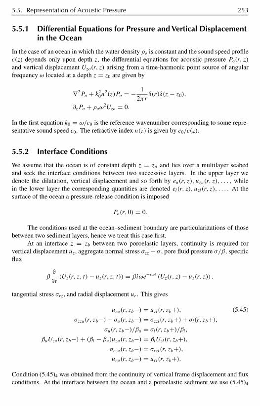
5.5. Representation of Acoustic Pressure 253
5.5.1 Differential Equations for Pressure and Vertical Displacementin the Ocean
In the case of an ocean in which the water density ρo is constant and the sound speed profilec(z) depends only upon depth z, the differential equations for acoustic pressure Po(r, z)and vertical displacement Uzo(r, z) arising from a time-harmonic point source of angularfrequency ω located at a depth z = z0 are given by
∇2Po + k20n
2(z)Po = − 1
2πrδ(r)δ(z− z0),
∂zPo + ρoω2Uzo = 0.
In the first equation k0 = ω/c0 is the reference wavenumber corresponding to some repre-sentative sound speed c0. The refractive index n(z) is given by c0/c(z).
5.5.2 Interface Conditions
We assume that the ocean is of constant depth z = zd and lies over a multilayer seabedand seek the interface conditions between two successive layers. In the upper layer wedenote the dilatation, vertical displacement and so forth by eu(r, z), uzu(r, z), . . . , whilein the lower layer the corresponding quantities are denoted el(r, z), uzl(r, z), . . . . At thesurface of the ocean a pressure-release condition is imposed
Po(r, 0) = 0.
The conditions used at the ocean–sediment boundary are particularizations of thosebetween two sediment layers, hence we treat this case first.
At an interface z = zb between two poroelastic layers, continuity is required forvertical displacement uz, aggregate normal stress σzz + σ , pore fluid pressure σ/β, specificflux
β∂
∂t(Uz(r, z, t)− uz(r, z, t)) = βiωe−iωt (Uz(r, z)− uz(r, z)) ,
tangential stress σrz, and radial displacement ur . This gives
uzu(r, zb−) = uzl(r, zb+), (5.45)
σzzu(r, zb−)+ σu(r, zb−) = σzzl(r, zb+)+ σl(r, zb+),σu(r, zb−)/βu = σl(r, zb+)/βl,
βuUzu(r, zb−)+ (βl − βu)uzu(r, zb−) = βlUzl(r, zb+),σrzu(r, zb−) = σrzl(r, zb+),uru(r, zb−) = url(r, zb+).
Condition (5.45)4 was obtained from the continuity of vertical frame displacement and fluxconditions. At the interface between the ocean and a poroelastic sediment we use (5.45)4

254 Chapter 5. Shallow Oceans over Poroelastic Seabeds
with β = 1 on the ocean side, equate both sediment side normal stress and pore stress toPo, and set tangential stress to zero on the ocean side. This gives
Uzo(r, zd−) = βsUzs(r, zd+)+ (1 − βs)uzs(r, zd+), (5.46)
Po(r, zd−) = σzzs(r, zd+)+ σs(r, zd+),Po(r, zd−) = σs(r, zd+)/βs,σrzs(r, zd+) = 0.
For a poroelastic layer over an elastic layer, continuity is required for both skele-tal and fluid vertical displacement, aggregate normal stress, tangential stress, and radialdisplacement. This gives
uzu(r, zb−) = Uzu(r, zb−) = uzl(r, zb+),σzzu(r, zb−)+ σu(r, zb−) = σzzl(r, zb+),
σrzu(r, zb−) = σrzl(r, zb+),uru(r, zb−) = url(r, zb+).
For an interface between two elastic layers we require continuity of vertical displace-ment uz, normal stress σzz, tangential stress σrz, and radial displacement ur . At the boundaryz = zb between the two elastic layers this gives
uzu(r, zb−) = uzl(r, zb+),σzzu(r, zb−) = σzzl(r, zb+),σrzu(r, zb−) = σrzl(r, zb+),uru(r, zb−) = url(r, zb+).
At the interface z = zd between the ocean and an elastic sediment, the radial displacementcondition is dropped and tangential stress is set to zero on the ocean side. This gives
Uzo(r, zd−) = uz(r, zd+),Po(r, zd−) = σzz(r, zd+),σrz(r, zd+) = 0.
The bottom-most, substrate layer will be treated as a half-space. We require as asymp-totic conditions that all dilatations and displacements vanish as z → ∞. Thus, if the top ofthe substrate layer is a distance zb from the ocean surface and it is poroelastic, the solutions(5.42) have the form
τ(z) = c1eim+(z−zb) + c3e
im−(z−zb), (5.47)
σ(z) = m2+B12
c1eim+(z−zb) + m2−
B12c3e
im−(z−zb) − a2τs
B12
(c1e
im+(z−zb) + c3eim−(z−zb)) ,
uz(z) = c1im+
(A32m
2+ − A32a2τ + A31B12
)B12
(m2+ − a2
u
) eim+(z−zb)

5.5. Representation of Acoustic Pressure 255
+ c3im−
(A32m
2− − A32a2τ + A31B12
)B12
(m2− − a2
u
) eim−(z−zb) + c5eiau(z−zb).
Similarly, for an elastic substrate we have from (5.44)
e = c1eia(z−zb),
uz = iCac1eia(z−zd )
a2 − b2+ c3e
ib(z−zd ).
5.5.3 Green’s Function Representation of Acoustic Pressure
We now construct a modal representation for acoustic pressure in the ocean, following theformulation presented in Boyles [52]. The process is similar irrespective of which model,elastic or poroelastic, is used for the sediment layers. We illustrate with the case of an oceanover a poroelastic half-space. More detail can be found in Buchanan, Gilbert, and Xu [84].A Green’s function representation
Po(r, z, z0) = k20
8π
∮C0
H(1)0 (k0
√κr)G2(z, z0, κ)dκ (5.48)
is sought. The contour C0 must enclose all singularities of G2 and exclude those ofH(1)0 (k0
√κr). We choose it to be the slit cut enclosing the positive real axis, oriented
counterclockwise. The depth Green’s function G2 then satisfies the differential equation
d2G2
dz2+ a2
oG2 = −δ(z− z0), (5.49)
where ao(z, κ) := k0
√n(z)2 − κ , with the interface conditions
G2(0, z0, κ) = 0 (5.50)
at the ocean surface and
G2(z0−, z0, κ) = G2(z0+, z0, κ),
dG2
dz(z0+, z0, κ)− dG2
dz(z0−, z0, κ) = −1 (5.51)
at the source depth.Let ϕ1(z, κ) and ϕ2(z, κ) be solutions to
d2ϕ
dz2+ a2
o(z, κ)ϕ = 0 (5.52)
satisfying the conditions
ϕ1(0, κ) = 0, ϕ′1(0, κ) = 1, (5.53)
ϕ2(0, κ) = 1, ϕ′2(0, κ) = 0.
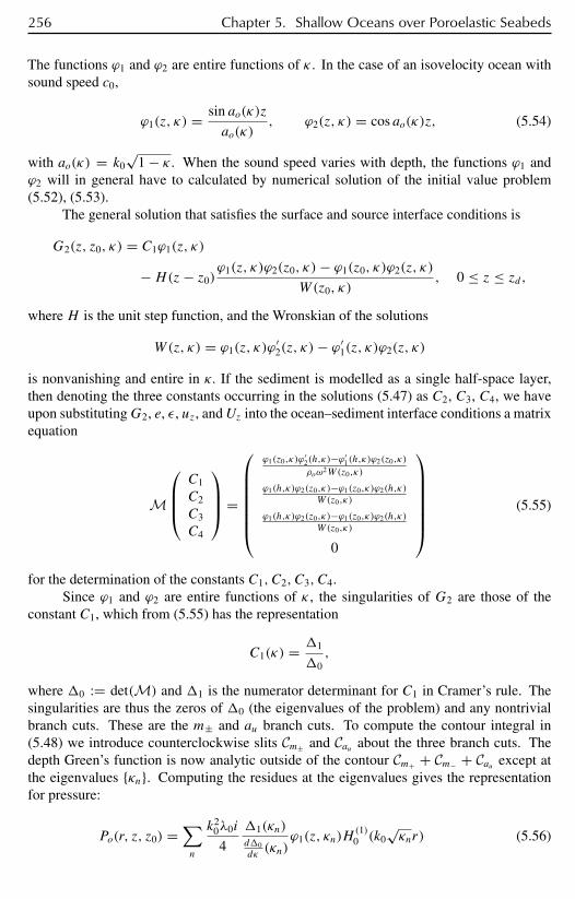
256 Chapter 5. Shallow Oceans over Poroelastic Seabeds
The functions ϕ1 and ϕ2 are entire functions of κ . In the case of an isovelocity ocean withsound speed c0,
ϕ1(z, κ) = sin ao(κ)z
ao(κ), ϕ2(z, κ) = cos ao(κ)z, (5.54)
with ao(κ) = k0√
1 − κ . When the sound speed varies with depth, the functions ϕ1 andϕ2 will in general have to calculated by numerical solution of the initial value problem(5.52), (5.53).
The general solution that satisfies the surface and source interface conditions is
G2(z, z0, κ) = C1ϕ1(z, κ)
−H(z− z0)ϕ1(z, κ)ϕ2(z0, κ)− ϕ1(z0, κ)ϕ2(z, κ)
W(z0, κ), 0 ≤ z ≤ zd,
where H is the unit step function, and the Wronskian of the solutions
W(z, κ) = ϕ1(z, κ)ϕ′2(z, κ)− ϕ′
1(z, κ)ϕ2(z, κ)
is nonvanishing and entire in κ. If the sediment is modelled as a single half-space layer,then denoting the three constants occurring in the solutions (5.47) as C2, C3, C4, we haveupon substitutingG2, e, ε, uz, andUz into the ocean–sediment interface conditions a matrixequation
M
C1
C2
C3
C4
=
ϕ1(z0,κ)ϕ′2(h,κ)−ϕ′
1(h,κ)ϕ2(z0,κ)
ρoω2W(z0,κ)
ϕ1(h,κ)ϕ2(z0,κ)−ϕ1(z0,κ)ϕ2(h,κ)
W(z0,κ)
ϕ1(h,κ)ϕ2(z0,κ)−ϕ1(z0,κ)ϕ2(h,κ)
W(z0,κ)
0
(5.55)
for the determination of the constants C1, C2, C3, C4.Since ϕ1 and ϕ2 are entire functions of κ , the singularities of G2 are those of the
constant C1, which from (5.55) has the representation
C1(κ) = 1
0,
where 0 := det(M) and 1 is the numerator determinant for C1 in Cramer’s rule. Thesingularities are thus the zeros of 0 (the eigenvalues of the problem) and any nontrivialbranch cuts. These are the m± and au branch cuts. To compute the contour integral in(5.48) we introduce counterclockwise slits Cm± and Cau about the three branch cuts. Thedepth Green’s function is now analytic outside of the contour Cm+ + Cm− + Cau except atthe eigenvalues κn. Computing the residues at the eigenvalues gives the representationfor pressure:
Po(r, z, z0) =∑n
k20λ0i
4
1(κn)d0dκ(κn)
ϕ1(z, κn)H(1)0 (k0
√κnr) (5.56)

5.6. Sound Transmission over a Poroelastic Half-Space 257
− k20
8π
∮Cm++Cm−+Cau
C1(κ)ϕ1(z, κ)H(1)0 (k0
√κr)dκ.
When the sediment has multiple layers, then in all layers except the bottom one thesolutions (5.42) can be written as
τ(z) = c1sinm+(z− zd)
m++ c2 cosm+(z− zd)+ c3
sinm−(z− zd)m−
+ c4 cosm−(z− zd)
and so forth, and thus the solutions are entire in κ . Therefore, the integrals in (5.56) need onlybe computed for the bottom, half-space, layer. It should be noted that while the solutionsτ , σ , and uz can in theory be calculated numerically, thereby permitting consideration ofsediments with depth-varying coefficients, this is not practical because the two solutionscorresponding to the twom+ terms in (5.47) undergo enormous variations in magnitude overeven a small change in depth, making accurate determination of their values difficult. Amore feasible approach for the case of depth-varying parameters is the numerical techniqueparabolic approximation. This method is discussed in Buchanan and Gilbert [78], but weshall not pursue it here.
5.6 Sound Transmission over a Poroelastic Half-SpaceIn section 5.4.2 we considered the effect of the parameters on the speeds and attenuationsof the different types of waves predicted by the Biot model. Investigating such effects hasbeen the primary concern of many of the articles cited. Perhaps more important but less wellstudied is the ability of the model to predict acoustic pressure. Of the articles cited, only[26] considers the Biot model’s predictions of acoustic pressure, and the model used therewas not an implementation of the full set of Biot equations. As seen in the previous section,it is possible to completely solve these equations in the case of constant seabed parameters.The predictions made by these solutions will be the concern of this and the next section.Let us first consider the predictions of (5.56) for an isovelocity ocean over a poroelastichalf-space. We shall use transmission loss as a measure of the strength of the acoustic fieldPo(r, z, z0). Transmission loss, normalized to be zero decibels 1m from a point source, is
T L = −20 log(4π |Po(r, z, z0)|). (5.57)
From (5.56) the total acoustic field consists of a discrete and a continuous spectrumterm. The eigenvalues κn in the discrete term are found numerically by minimizing|0(κ)|, since this is found to be more reliable than solving 0(κ) = 0 numerically. Thederivatives d0
dκ(κn) in the discrete spectrum term and the integrals along the branch cuts
in the continuous spectrum term are computed numerically. At very low frequencies thereare no eigenvalues, and hence all the energy is in the continuous spectrum. The frequencyat which the first eigenvalue emerges is the modal cutoff . As the frequency increases,more and more of the energy in the field shifts to the discrete spectrum. The mathematicalmechanism for this shift is the emergence of eigenvalues from the branch cuts at certainfrequencies. Having emerged from the branch cut the eigenvalues migrate toward the pointκ = 1 (Figure 5.32 (top)). The clustering of the eigenvalues near κ = 1 means that locating
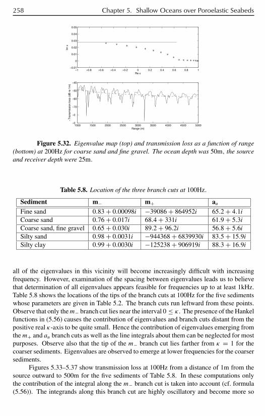
258 Chapter 5. Shallow Oceans over Poroelastic Seabeds
−1 −0.8 −0.6 −0.4 −0.2 0 0.2 0.4 0.6 0.8 1−0.01
0
0.01
0.02
0.03
0.04
0.05
Re κ
Im κ
1000 1500 2000 2500 3000 3500 4000 4500 5000−90
−80
−70
−60
−50
−40
Range (m)
−T
rans
mis
sion
loss
(dB
re
1m)
Figure 5.32. Eigenvalue map (top) and transmission loss as a function of range(bottom) at 200Hz for coarse sand and fine gravel. The ocean depth was 50m, the sourceand receiver depth were 25m.
Table 5.8. Location of the three branch cuts at 100Hz.
Sediment m− m+ auFine sand 0.83 + 0.00098i −39086 + 864952i 65.2 + 4.1iCoarse sand 0.76 + 0.017i 68.4 + 331i 61.9 + 5.3iCoarse sand, fine gravel 0.65 + 0.030i 89.2 + 96.2i 56.8 + 5.6iSilty sand 0.98 + 0.0031i −944368 + 6839930i 83.5 + 15.9iSilty clay 0.99 + 0.0030i −125238 + 906919i 88.3 + 16.9i
all of the eigenvalues in this vicinity will become increasingly difficult with increasingfrequency. However, examination of the spacing between eigenvalues leads us to believethat determination of all eigenvalues appears feasible for frequencies up to at least 1kHz.Table 5.8 shows the locations of the tips of the branch cuts at 100Hz for the five sedimentswhose parameters are given in Table 5.2. The branch cuts run leftward from these points.Observe that only them− branch cut lies near the interval 0 ≤ κ . The presence of the Hankelfunctions in (5.56) causes the contribution of eigenvalues and branch cuts distant from thepositive real κ-axis to be quite small. Hence the contribution of eigenvalues emerging fromthem+ and au branch cuts as well as the line integrals about them can be neglected for mostpurposes. Observe also that the tip of the m− branch cut lies farther from κ = 1 for thecoarser sediments. Eigenvalues are observed to emerge at lower frequencies for the coarsersediments.
Figures 5.33–5.37 show transmission loss at 100Hz from a distance of 1m from thesource outward to 500m for the five sediments of Table 5.8. In these computations onlythe contribution of the integral along the m− branch cut is taken into account (cf. formula(5.56)). The integrands along this branch cut are highly oscillatory and become more so
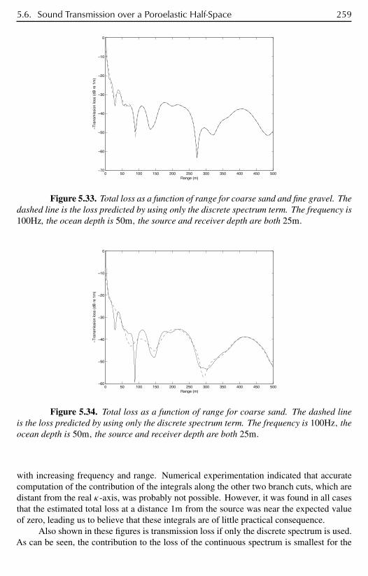
5.6. Sound Transmission over a Poroelastic Half-Space 259
0 50 100 150 200 250 300 350 400 450 500−70
−60
−50
−40
−30
−20
−10
0
Range (m)
−T
rans
mis
sion
loss
(dB
re
1m)
Figure 5.33. Total loss as a function of range for coarse sand and fine gravel. Thedashed line is the loss predicted by using only the discrete spectrum term. The frequency is100Hz, the ocean depth is 50m, the source and receiver depth are both 25m.
0 50 100 150 200 250 300 350 400 450 500−60
−50
−40
−30
−20
−10
0
Range (m)
−T
rans
mis
sion
loss
(dB
re
1m)
Figure 5.34. Total loss as a function of range for coarse sand. The dashed lineis the loss predicted by using only the discrete spectrum term. The frequency is 100Hz, theocean depth is 50m, the source and receiver depth are both 25m.
with increasing frequency and range. Numerical experimentation indicated that accuratecomputation of the contribution of the integrals along the other two branch cuts, which aredistant from the real κ-axis, was probably not possible. However, it was found in all casesthat the estimated total loss at a distance 1m from the source was near the expected valueof zero, leading us to believe that these integrals are of little practical consequence.
Also shown in these figures is transmission loss if only the discrete spectrum is used.As can be seen, the contribution to the loss of the continuous spectrum is smallest for the
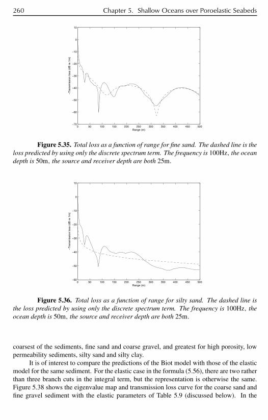
260 Chapter 5. Shallow Oceans over Poroelastic Seabeds
0 50 100 150 200 250 300 350 400 450 500−70
−60
−50
−40
−30
−20
−10
0
10
Range (m)
−T
rans
mis
sion
loss
(dB
re
1m)
Figure 5.35. Total loss as a function of range for fine sand. The dashed line is theloss predicted by using only the discrete spectrum term. The frequency is 100Hz, the oceandepth is 50m, the source and receiver depth are both 25m.
0 50 100 150 200 250 300 350 400 450 500−60
−50
−40
−30
−20
−10
0
10
Range (m)
−T
rans
mis
sion
loss
(dB
re
1m)
Figure 5.36. Total loss as a function of range for silty sand. The dashed line isthe loss predicted by using only the discrete spectrum term. The frequency is 100Hz, theocean depth is 50m, the source and receiver depth are both 25m.
coarsest of the sediments, fine sand and coarse gravel, and greatest for high porosity, lowpermeability sediments, silty sand and silty clay.
It is of interest to compare the predictions of the Biot model with those of the elasticmodel for the same sediment. For the elastic case in the formula (5.56), there are two ratherthan three branch cuts in the integral term, but the representation is otherwise the same.Figure 5.38 shows the eigenvalue map and transmission loss curve for the coarse sand andfine gravel sediment with the elastic parameters of Table 5.9 (discussed below). In the
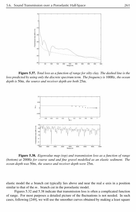
5.6. Sound Transmission over a Poroelastic Half-Space 261
0 50 100 150 200 250 300 350 400 450 500−60
−50
−40
−30
−20
−10
0
10
Range (m)
−T
rans
mis
sion
loss
(dB
re
1m)
Figure 5.37. Total loss as a function of range for silty clay. The dashed line is theloss predicted by using only the discrete spectrum term. The frequency is 100Hz, the oceandepth is 50m, the source and receiver depth are both 25m.
−1 −0.8 −0.6 −0.4 −0.2 0 0.2 0.4 0.6 0.8 1
−0.05
0
0.05
0.1
Re κ
Im κ
1000 1500 2000 2500 3000 3500 4000 4500 5000−100
−90
−80
−70
−60
−50
−40
Range (m)
−T
rans
mis
sion
loss
(dB
re
1m)
Figure 5.38. Eigenvalue map (top) and transmission loss as a function of range(bottom) at 200Hz for coarse sand and fine gravel modelled as an elastic sediment. Theocean depth was 50m, the source and receiver depth were 25m.
elastic model the a branch cut typically lies above and near the real κ-axis in a positionsimilar to that of the m− branch cut in the poroelastic model.
Figures 5.32 and 5.38 indicate that transmission loss is often a complicated functionof range. For most purposes a detailed picture of the fluctuations is not needed. In suchcases, following [249], we will use the smoother curves obtained by making a least square
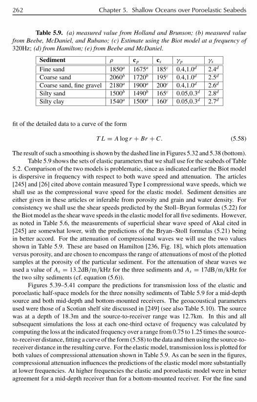
262 Chapter 5. Shallow Oceans over Poroelastic Seabeds
Table 5.9. (a) measured value from Holland and Brunson; (b) measured valuefrom Beebe, McDaniel, and Rubano; (c) Estimate using the Biot model at a frequency of320Hz; (d) from Hamilton; (e) from Beebe and McDaniel.
Sediment ρ cp cs γp γs
Fine sand 1850a 1675a 185c 0.4,1.0d 2.4d
Coarse sand 2060b 1720b 195c 0.4,1.0d 2.5d
Coarse sand, fine gravel 2180a 1900a 200c 0.4,1.0d 2.6d
Silty sand 1500b 1490b 165c 0.05,0.3d 2.8d
Silty clay 1540a 1500a 160c 0.05,0.3d 2.7d
fit of the detailed data to a curve of the form
T L = A log r + Br + C. (5.58)
The result of such a smoothing is shown by the dashed line in Figures 5.32 and 5.38 (bottom).Table 5.9 shows the sets of elastic parameters that we shall use for the seabeds of Table
5.2. Comparison of the two models is problematic, since as indicated earlier the Biot modelis dispersive in frequency with respect to both wave speed and attenuation. The articles[245] and [26] cited above contain measured Type I compressional wave speeds, which weshall use as the compressional wave speed for the elastic model. Sediment densities areeither given in these articles or inferable from porosity and grain and water density. Forconsistency we shall use the shear speeds predicted by the Stoll–Bryan formulas (5.22) forthe Biot model as the shear wave speeds in the elastic model for all five sediments. However,as noted in Table 5.6, the measurements of superficial shear wave speed of Akal cited in[245] are somewhat lower, with the predictions of the Bryan–Stoll formulas (5.21) beingin better accord. For the attenuation of compressional waves we will use the two valuesshown in Table 5.9. These are based on Hamilton [236, Fig. 18], which plots attenuationversus porosity, and are chosen to encompass the range of attenuations of most of the plottedsamples at the porosity of the particular sediment. For the attenuation of shear waves weused a value of As = 13.2dB/m/kHz for the three sediments and As = 17dB/m/kHz forthe two silty sediments (cf. equation (5.6)).
Figures 5.39–5.41 compare the predictions for transmission loss of the elastic andporoelastic half-space models for the three nonsilty sediments of Table 5.9 for a mid-depthsource and both mid-depth and bottom-mounted receivers. The geoacoustical parametersused were those of a Scotian shelf site discussed in [249] (see also Table 5.10). The sourcewas at a depth of 18.3m and the source-to-receiver range was 12.7km. In this and allsubsequent simulations the loss at each one-third octave of frequency was calculated bycomputing the loss at the indicated frequency over a range from 0.75 to 1.25 times the source-to-receiver distance, fitting a curve of the form (5.58) to the data and then using the source-to-receiver distance in the resulting curve. For the elastic model, transmission loss is plotted forboth values of compressional attenuation shown in Table 5.9. As can be seen in the figures,compressional attenuation influences the predictions of the elastic model more substantiallyat lower frequencies. At higher frequencies the elastic and poroelastic model were in betteragreement for a mid-depth receiver than for a bottom-mounted receiver. For the fine sand
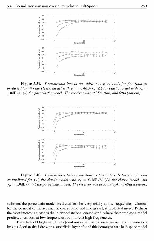
5.6. Sound Transmission over a Poroelastic Half-Space 263
101
102
103
−120
−110
−100
−90
−80
−70
−60
−50
Frequency (Hz)
−T
rans
mis
sion
loss
(dB
re
1m)
101
102
103
−120
−110
−100
−90
−80
−70
−60
−50
Frequency (Hz)
−T
rans
mis
sion
loss
(dB
re
1m)
Figure 5.39. Transmission loss at one-third octave intervals for fine sand aspredicted for () the elastic model with γp = 0.4dB/λ; () the elastic model with γp =1.0dB/λ; () the poroelastic model. The receiver was at 35m (top) and 69m (bottom).
101
102
103
−120
−110
−100
−90
−80
−70
−60
−50
Frequency (Hz)
−T
rans
mis
sion
loss
(dB
re
1m)
101
102
103
−120
−110
−100
−90
−80
−70
−60
−50
Frequency (Hz)
−T
rans
mis
sion
loss
(dB
re
1m)
Figure 5.40. Transmission loss at one-third octave intervals for coarse sandas predicted for () the elastic model with γp = 0.4dB/λ; () the elastic model withγp = 1.0dB/λ; () the poroelastic model. The receiver was at 35m (top) and 69m (bottom).
sediment the poroelastic model predicted less loss, especially at low frequencies, whereasfor the coarsest of the sediments, coarse sand and fine gravel, it predicted more. Perhapsthe most interesting case is the intermediate one, coarse sand, where the poroelastic modelpredicted less loss at low frequencies, but more at high frequencies.
The article of Hughes et al. [249] contains experimental measurements of transmissionloss at a Scotian shelf site with a superficial layer of sand thick enough that a half-space model
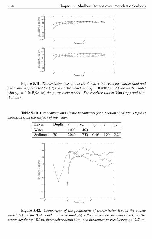
264 Chapter 5. Shallow Oceans over Poroelastic Seabeds
101
102
103
−120
−110
−100
−90
−80
−70
−60
−50
Frequency (Hz)
−T
rans
mis
sion
loss
(dB
re
1m)
101
102
103
−120
−110
−100
−90
−80
−70
−60
−50
Frequency (Hz)
−T
rans
mis
sion
loss
(dB
re
1m)
Figure 5.41. Transmission loss at one-third octave intervals for coarse sand andfine gravel as predicted for () the elastic model with γp = 0.4dB/λ; () the elastic modelwith γp = 1.0dB/λ; () the poroelastic model. The receiver was at 35m (top) and 69m(bottom).
Table 5.10. Geoacoustic and elastic parameters for a Scotian shelf site. Depth ismeasured from the surface of the water.
Layer Depth ρ cp γp cs γs
Water 1000 1460Sediment 70 2060 1750 0.46 170 2.2
100
101
102
103
−100
−95
−90
−85
−80
−75
−70
−65
−60
Frequency (Hz)
−T
rans
mis
sion
loss
(dB
re
1m)
Figure 5.42. Comparison of the predictions of transmission loss of the elasticmodel () and the Biot model for coarse sand ()with experimental measurement (). Thesource depth was 18.3m, the receiver depth 69m, and the source-to-receiver range 12.7km.
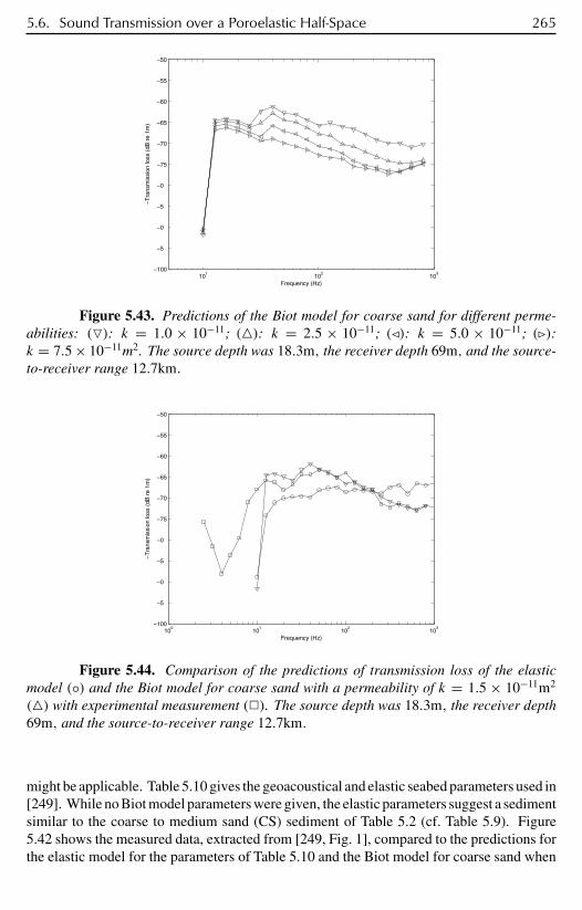
5.6. Sound Transmission over a Poroelastic Half-Space 265
101
102
103
−100
−95
−90
−85
−80
−75
−70
−65
−60
−55
−50
Frequency (Hz)
−T
rans
mis
sion
loss
(dB
re
1m)
Figure 5.43. Predictions of the Biot model for coarse sand for different perme-abilities: (): k = 1.0 × 10⁻¹¹; (): k = 2.5 × 10⁻¹¹; ()): k = 5.0 × 10⁻¹¹; (*):k = 7.5 × 10⁻¹¹m2. The source depth was 18.3m, the receiver depth 69m, and the source-to-receiver range 12.7km.
100
101
102
103
−100
−95
−90
−85
−80
−75
−70
−65
−60
−55
−50
Frequency (Hz)
−T
rans
mis
sion
loss
(dB
re
1m)
Figure 5.44. Comparison of the predictions of transmission loss of the elasticmodel () and the Biot model for coarse sand with a permeability of k = 1.5 × 10⁻¹¹m2
() with experimental measurement (). The source depth was 18.3m, the receiver depth69m, and the source-to-receiver range 12.7km.
might be applicable. Table 5.10 gives the geoacoustical and elastic seabed parameters used in[249]. While no Biot model parameters were given, the elastic parameters suggest a sedimentsimilar to the coarse to medium sand (CS) sediment of Table 5.2 (cf. Table 5.9). Figure5.42 shows the measured data, extracted from [249, Fig. 1], compared to the predictions forthe elastic model for the parameters of Table 5.10 and the Biot model for coarse sand when
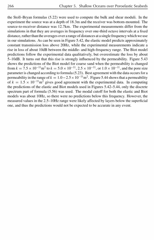
266 Chapter 5. Shallow Oceans over Poroelastic Seabeds
the Stoll–Bryan formulas (5.22) were used to compute the bulk and shear moduli. In theexperiment the source was at a depth of 18.3m and the receiver was bottom-mounted. Thesource-to-receiver distance was 12.7km. The experimental measurements differ from thesimulations in that they are averages in frequency over one-third octave intervals at a fixeddistance, rather than the averages over a range of distances at a single frequency which we usein our simulations. As can be seen in Figure 5.42, the elastic model predicts approximatelyconstant transmission loss above 20Hz, while the experimental measurements indicate arise in loss of about 10dB between the middle- and high-frequency range. The Biot modelpredictions follow the experimental data qualitatively, but overestimate the loss by about5–10dB. It turns out that this rise is strongly influenced by the permeability. Figure 5.43shows the predictions of the Biot model for coarse sand when the permeability is changedfrom k = 7.5 × 10⁻¹¹m2 to k = 5.0 × 10⁻¹¹, 2.5 × 10⁻¹¹, or 1.0 × 10⁻¹¹, and the pore sizeparameter is changed according to formula (5.23). Best agreement with the data occurs for apermeability in the range of k = 1.0−2.5×10⁻¹¹m2. Figure 5.44 shows that a permeabilityof k = 1.5 × 10⁻¹¹m2 gives good agreement with the experimental data. In computingthe predictions of the elastic and Biot models used in Figures 5.42–5.44, only the discretespectrum part of formula (5.56) was used. The modal cutoff for both the elastic and Biotmodels was about 10Hz, so there were no predictions below this frequency. However, themeasured values in the 2.5–10Hz range were likely affected by layers below the superficialone, and thus the predictions would not be expected to be accurate in any event.
Chapter 6
Homogenization of theSeabed and OtherAsymptotic Methods
6.1 Low Shear Asymptotics for Elastic SeabedsIn this section on small shear asymptotics, we find it convenient to have the ocean surfaceat z = −h, the bottom at z = 0, and the seabed lying in the region z > 0. For simplicitywe treat only the case of a 2D ocean–seabed system.
In this section we report on the work of Gilbert and Makrakis [188] on the asymptoticbehavior of 2D time-harmonic acoustic waves in an ocean lying on an elastic seabed, wherethe modulus of the shear modulus is small compared with its bulk modulus.
We assume that the ocean D = (x, z)|x ∈ R, −h ≤ z ≤ 0 is filled by an idealacoustic fluid with constant density ρf , while the bottom is filled by a homogeneous andisotropic elastic material, with Lamè constants λ,µ and density ρ. The compressional andshear wave velocities are cp = √
(λ+ 2µ)/ρ and cs = √µ/ρ.
Under the above assumptions, the pressure in the ocean is governed by the Helmholtzequation and we assume, as customary, that the surface is pressure released.
Let u, v be the displacements of the elastic bottom B = (x, z)|x ∈ R, z ≥ 0 in thedirections x, z, respectively. For an isotropic medium the stresses σxx, σzz, σxz are given interms of the displacements by the relations
σxx = (λ+ 2µ)∂xu+ λ∂zv,σzz = λ∂xu+ (λ+ 2µ)∂zv,
σxz = µ(∂zu+ ∂xu).Recalling Chapter 4, the equations of motion in terms of the stresses are given by
∂xσxx + ∂zσxz + ρω2u = 0, ∂xσxz + ∂zσzz + ρω2v = 0,
while in terms of the displacements $u = (u, v), they satisfy
µ$u+ (λ+ µ)∇(∇$u)+ ρω2$u = 0. (6.1)
The usual continuity conditions are satisfied on the interface between the ocean and
267
268 Chapter 6. Homogenization of the Seabed and Other Asymptotic Methods
the seabed, namely,
σxz(x, 0) = 0, σzz(x, 0) = −p(x, 0), x ∈ R. (6.2)
It is convenient to formulate the problem in terms of the Lamé displacement potentials φand ψ . These potentials are related to the displacements by
u = ∂xφ + ∂zψ, v = ∂zφ − ∂xψ. (6.3)
In terms of these potentials the equations of motion are equivalent to the Helmholtz equations
φ + k2s φ = 0, ψ + k2
pψ = 0, (6.4)
and kp = ω/cp, ks = ω/cs are the compressional and shear wavenumbers, respectively.By introducing the Love function L, which is related to the displacements by15
u = −λ+ µµ
∂2xzL, v = λ+ µ
µ∂2xL+ ∂2
z L+ ρω2
µL, (6.5)
the equations of motion are equivalent to the metaharmonic equation
LεL = ε(2L+ k2L)+ k2(L+ k2L) = 0, (6.6)
where
ε = (cp/cs)2 = µ/(λ+ 2µ).
In terms of the Love function, the stresses are given by
σxx = (ρc2p)∂z((1 − 2ε)(L+ ε−1k2L)− 2(1 − ε)∂2
xL), (6.7)
σzz = (ρc2p)∂z((1 − 2ε)(L+ ε−1k2L)+ 2(L+ k2L)− 2(1 − ε)∂2
z L), (6.8)
σxz = (ρc2p)∂x((L+ k2L)− 2(1 − ε)∂2
z L). (6.9)
We observe that as µ → 0, the Navier system (6.1) leads formally to a singularperturbation problem, while from (6.9) it follows that the zero shear condition is triviallysatisfied. In the Lamé potential formulation, we observe that only the equation for thepotential ψ becomes a singular perturbation, while the zero shear boundary condition isagain trivially satisfied. In the formulation with the Love function, the metaharmonicequation (6.9) leads to a singular perturbation, as it reduces to the Helmholtz equation forL as ε → 0, and the conditions (6.7), (6.8), and (6.9) imply that σxz = 0, whereas σxx, σzzremain finite on the boundary y = 0 only if σxx = 0 = σzz on z = 0, which is a trivial case.In the formal limit ε = 0, the compressional velocity cp tends to c0 = √
λ/ρ, and we put
k20 = ω2
c20
= ρω2
λ.
Following physical considerations, we anticipate that the limit under investigationmust correspond to a fluid seabed, which suggests that the shear boundary condition shouldbecome trivial. In fact, it turns out that one of the elastodynamic equations plays the roleof a kinematic constraint. In the next subsection we investigate the singular perturbationnature starting with the displacement formulation, which is the most natural one.
15See [347], [354], [395].
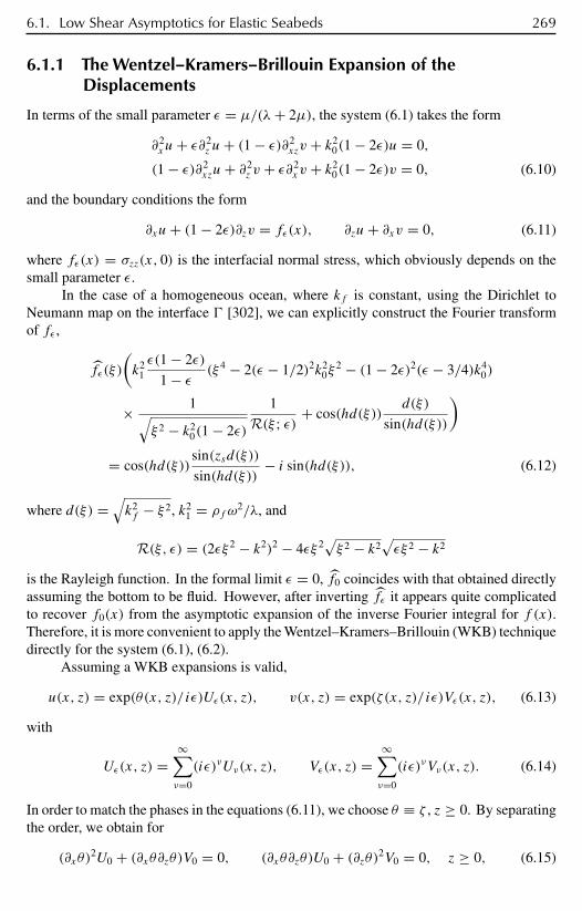
6.1. Low Shear Asymptotics for Elastic Seabeds 269
6.1.1 The Wentzel–Kramers–Brillouin Expansion of theDisplacements
In terms of the small parameter ε = µ/(λ+ 2µ), the system (6.1) takes the form
∂2xu+ ε∂2
z u+ (1 − ε)∂2xzv + k2
0(1 − 2ε)u = 0,
(1 − ε)∂2xzu+ ∂2
z v + ε∂2x v + k2
0(1 − 2ε)v = 0, (6.10)
and the boundary conditions the form
∂xu+ (1 − 2ε)∂zv = fε(x), ∂zu+ ∂xv = 0, (6.11)
where fε(x) = σzz(x, 0) is the interfacial normal stress, which obviously depends on thesmall parameter ε.
In the case of a homogeneous ocean, where kf is constant, using the Dirichlet toNeumann map on the interface [302], we can explicitly construct the Fourier transformof fε ,
fε(ξ)
(k2
1ε(1 − 2ε)
1 − ε (ξ 4 − 2(ε − 1/2)2k20ξ
2 − (1 − 2ε)2(ε − 3/4)k40)
× 1√ξ 2 − k2
0(1 − 2ε)
1
R(ξ ; ε) + cos(hd(ξ))d(ξ)
sin(hd(ξ))
)
= cos(hd(ξ))sin(zsd(ξ))
sin(hd(ξ))− i sin(hd(ξ)), (6.12)
where d(ξ) =√k2f − ξ 2, k2
1 = ρf ω2/λ, and
R(ξ, ε) = (2εξ 2 − k2)2 − 4εξ 2√ξ 2 − k2
√εξ 2 − k2
is the Rayleigh function. In the formal limit ε = 0, f0 coincides with that obtained directlyassuming the bottom to be fluid. However, after inverting fε it appears quite complicatedto recover f0(x) from the asymptotic expansion of the inverse Fourier integral for f (x).Therefore, it is more convenient to apply the Wentzel–Kramers–Brillouin (WKB) techniquedirectly for the system (6.1), (6.2).
Assuming a WKB expansions is valid,
u(x, z) = exp(θ(x, z)/iε)Uε(x, z), v(x, z) = exp(ζ(x, z)/iε)Vε(x, z), (6.13)
with
Uε(x, z) =∞∑ν=0
(iε)νUν(x, z), Vε(x, z) =∞∑ν=0
(iε)νVν(x, z). (6.14)
In order to match the phases in the equations (6.11), we choose θ ≡ ζ , z ≥ 0. By separatingthe order, we obtain for
(∂xθ)2U0 + (∂xθ∂zθ)V0 = 0, (∂xθ∂zθ)U0 + (∂zθ)2V0 = 0, z ≥ 0, (6.15)

270 Chapter 6. Homogenization of the Seabed and Other Asymptotic Methods
and
(∂zθ)U0 + (∂xθ)V0 = 0, (∂xθ)U0 + (∂xθ)V0 = 0, z = 0. (6.16)
Obviously (6.15) can have nontrivial solutions since the determinant of the system forU0, V0
is zero, and the boundary conditions (6.16) can be satisfied if (∂zθ)2 − (∂xθ)2 = 0 for z = 0.On the other hand, all these conditions are trivially satisfied for θ = 0, which should be thecase when the source term in the nonhomogeneous Helmholtz equation, which describesthe signal in the ocean, does not contain an oscillatory term like exp(θ/iε). Therefore, theproblem at hand is a regular perturbation problem.
6.1.2 The Regular Perturbation Expansion
We now assume that the displacements and the normal boundary traction have the followingregular perturbation expansion:
u(x, z) =∞∑ν=0
ενuν(x, z), v(x, z) =∞∑ν=0
ενvν(x, z), f (x) =∞∑ν=0
ενfν(x),
(6.17)
where ε = cs/cp. Substituting these expansions into the equations of motion (6.1), andseparating the various orders, we obtain the following hierarchy of equations in B:
∂2xu0 + ∂2
xzv0 + k20u0 = 0, ∂2
z v0 + ∂2xzu0 + k2
0v0 = 0, (6.18)
∂2xuν + ∂2
xzvν + k20uν = ∂2
xzvν−1 − ∂2z vν−1 + 2k2
0uν−1 (6.19)
∂2z vν + ∂2
xzuν + k20vν = ∂2
xzuν−1 − ∂2x vν−1 + 2k2
0vν−1, ν ≥ 1, (6.20)
where k20 = ρω2/λ. Moreover, substituting the expansions (6.17) into the boundary con-
ditions (6.7), (6.9), (6.8) we construct the corresponding boundary conditions on z = 0,namely,
∂xu0 + ∂zv0 = f0, (6.21)
∂xuν + ∂zvν = 2∂zvν−1 + fν − 2fν−1, ν ≥ 1, (6.22)
from the normal stress, and
g0 = 0, ∂zu0 + ∂xv0 = g1, (6.23)
∂zuν−1 + ∂xvν−1 = gν − 2gν−1, ν ≥ 2, (6.24)
from the zero shear stress.First we consider the zeroth-order system (6.18), (6.21), and (6.24). Moreover, let
"ν = ∂xuν + ∂zvν, Wν = ∂zuν − ∂xvν (6.25)
be the dilation and the rotation corresponding to the displacements (uν, vν). By differenti-ating the equations (6.18) with respect to x, z, respectively, we find that
"0 + k20"0 = 0, W0 = 0, (6.26)

6.1. Low Shear Asymptotics for Elastic Seabeds 271
which is to say that the displacement field (u0, v0) is rotation free. This corresponds to thefluid limit, as ε → 0. Using now the condition W0 = 0 as a kinematic constraint in theform ∂zu0 = ∂xv0, we rewrite (6.18) as a decoupled system:
u0 + k20u0 = 0, v0 + k2
0v0 = 0, (6.27)
which satisfies the coupled boundary conditions (6.21) and (6.23).Similarly, we can show that the (uν, vν), ν ≥ 1 satisfy the uncoupled equations
uν + k20uν = 2∂zWν−1 + k−2
0 ∂z(∂xWν−1 + ∂2
z (∂xvν−1 − ∂zvν1))
+ ∂2xzvν−1 − ∂2
z vν−1 + 2k20uν−1, (6.28)
vν + k20vν = 2∂xWν−1 + k−2
0 ∂x(∂2xWν−1 + ∂2
z (∂xvν−1 − ∂zvν−1))
+ ∂2xzuν−1 − ∂2
x vν−1 + 2k20vν−1. (6.29)
The above systems for uν, vν , can be solved by using Fourier transform methods andthe correct radiation conditions as z → ∞. For example, for the zeroth-order displacementswe find
u0(x, z) = − i
2π
∫ ∞
−∞f0(ξ)
ξ
2ξ 2 − k20
exp
(−iξx − z
√ξ 2 − k2
0
)dξ, (6.30)
v0(x, z) = − 1
2π
∫ ∞
−∞f0(ξ)
√ξ 2 − k2
0
2ξ 2 − k20
exp
(−iξx − z
√ξ 2 − k2
0
)dξ, (6.31)
where f0(ξ) = ∫∞−∞ exp(ixξ)f0(x)dx is the Fourier transform of the boundary traction
f0(x), given by
f0(ξ) = sin(d(ξ)h)
d(ξ)
(sin(d(ξ)zs)
sin(d(ξ)h)− i tan(d(ξ)h)
). (6.32)
The analysis of this section and the expressions (1.7) for the displacements in terms of theLamé potentials suggest that a similar regular perturbation expansion can be constructedusing the potential formulation. The constructed regular perturbation for the elastodynamicfield in the bottom leads to a regular perturbation expansion for the pressure field p =p(x, z), the zeroth-order term of which coincides with that corresponding to the limitingfluid bottom.
6.1.3 A Singular Perturbation Problem for the Love Function
Introducing the new unknown l byL = εl and putting µ = ελ/(1−2ε), we see that l againsatisfies the metaharmonic equation (6.6), and we rewrite the displacements (6.5) and thestresses (6.7)–(6.9) in the form
u = −(1 − ε)∂2xzl, v = (1 − ε)∂2
x l + ε∂2z l + k2
0(1 − 2ε)l, (6.33)
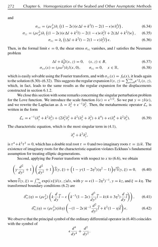
272 Chapter 6. Homogenization of the Seabed and Other Asymptotic Methods
and
σxx = (ρc2p)∂z
((1 − 2ε)(εl + k2l)− 2(1 − ε)ε∂2
x l), (6.34)
σzz = (ρc2p)∂z
((1 − 2ε)(εl + k2l)− 2(1 − ε)ε∂2
z l + 2(l + k2l)ε), (6.35)
σxz = ∂x((l + k2l)− 2(1 − ε)∂2
z l)ε. (6.36)
Then, in the formal limit ε = 0, the shear stress σxz vanishes, and l satisfies the Neumannproblem
l + k20 l(x, z) = 0, (x, z) ∈ B, (6.37)
σxx(x) = (ρω2)∂zl(x, 0), σxz = 0, x ∈ R, (6.38)
which is easily solvable using the Fourier transform, and with σzz(x) = f0(x), it leads againto the solution (6.30)–(6.32). This suggests the regular expansion l(x, z) = ∑∞
ν=0ενlν(x, z),
which, in fact, leads to the same results as the regular expansion for the displacementsconstructed in section 6.1.2.
We close this section with some remarks concerning the singular perturbation problemfor the Love function. We introduce the scale function δ(ε) = ε1/2. So we put y = zδ(ε),and we rewrite the Laplacian as = ∂2
x + ε−1∂2y . Then, the metaharmonic operator Lε is
written in the form
Lε = ε−1(∂4y + k2∂2
y )+ (2∂2x ∂
2y + k2(∂2
x + ∂2y )+ k4)+ ε(∂4
x + k2∂2x ). (6.39)
The characteristic equation, which is the most singular term in (4.1),
∂4y + k2∂2
y ,
is τ 4 +k2τ 2 = 0, which has a double real root τ = 0 and two imaginary roots τ = ±ik. Theexistence of imaginary roots for the characteristic equation violates Eckhaus’s fundamentalassumption for treating elliptic degenerations.
Second, applying the Fourier transform with respect to x to (6.6), we obtain(γd2
dy2+ 1
)(d2
dy2+ 1
)l(y, ξ)+
(1 − γ (1 − 2η2)(η2 − 1)
)η2l(y, ξ) = 0, (6.40)
where l(y, ξ) = ∫∞−∞ exp(ixξ)l(x, z)dx, with γ = ε(1−2η2)−1, y = kz, and ξ = kη. The
transformed boundary conditions (6.2) are
σzz(η) = (ρc2p)
(kd
dyl − ε
(k−3(1 − 2ε)
d3
dy3l − k(4 + 3η2)
d
dyl
)), (6.41)
σxz(η) = (ρc2p)(ikη)
(−(1 − 2ε)k−2 d
2
dy2l + k2(1 − η)l
)ε. (6.42)
We observe that the principal symbol of the ordinary differential operator in (6.40) coincideswith the symbol of
εd4
dy4+ d2
dy2.
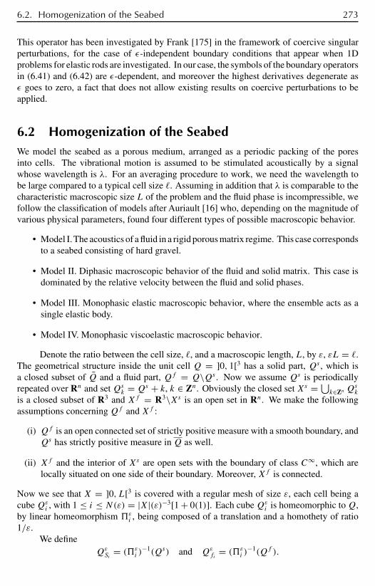
6.2. Homogenization of the Seabed 273
This operator has been investigated by Frank [175] in the framework of coercive singularperturbations, for the case of ε-independent boundary conditions that appear when 1Dproblems for elastic rods are investigated. In our case, the symbols of the boundary operatorsin (6.41) and (6.42) are ε-dependent, and moreover the highest derivatives degenerate asε goes to zero, a fact that does not allow existing results on coercive perturbations to beapplied.
6.2 Homogenization of the SeabedWe model the seabed as a porous medium, arranged as a periodic packing of the poresinto cells. The vibrational motion is assumed to be stimulated acoustically by a signalwhose wavelength is λ. For an averaging procedure to work, we need the wavelength tobe large compared to a typical cell size . Assuming in addition that λ is comparable to thecharacteristic macroscopic size L of the problem and the fluid phase is incompressible, wefollow the classification of models after Auriault [16] who, depending on the magnitude ofvarious physical parameters, found four different types of possible macroscopic behavior.
• Model I. The acoustics of a fluid in a rigid porous matrix regime. This case correspondsto a seabed consisting of hard gravel.
• Model II. Diphasic macroscopic behavior of the fluid and solid matrix. This case isdominated by the relative velocity between the fluid and solid phases.
• Model III. Monophasic elastic macroscopic behavior, where the ensemble acts as asingle elastic body.
• Model IV. Monophasic viscoelastic macroscopic behavior.
Denote the ratio between the cell size, , and a macroscopic length, L, by ε, εL = .The geometrical structure inside the unit cell Q = ]0, 1[3 has a solid part, Qs , which isa closed subset of Q and a fluid part, Qf = Q\Qs . Now we assume Qs is periodicallyrepeated over Rn and setQsk = Qs + k, k ∈ Zn. Obviously the closed set Xs = ⋃
k∈Zn Qsk
is a closed subset of R3 and Xf = R3\Xs is an open set in Rn. We make the followingassumptions concerningQf and Xf :
(i) Qf is an open connected set of strictly positive measure with a smooth boundary, andQs has strictly positive measure inQ as well.
(ii) Xf and the interior of Xs are open sets with the boundary of class C∞, which arelocally situated on one side of their boundary. Moreover, Xf is connected.
Now we see that X = ]0, L[3 is covered with a regular mesh of size ε, each cell being acubeQεi , with 1 ≤ i ≤ N(ε) = |X|(ε)−3[1 + 0(1)]. Each cubeQεi is homeomorphic toQ,by linear homeomorphism #εi , being composed of a translation and a homothety of ratio1/ε.
We defineQεSi = (#εi )
−1(Qs) and Qεfi = (#εi )−1(Qf ).

274 Chapter 6. Homogenization of the Seabed and Other Asymptotic Methods
For sufficiently small ε > 0 we consider the sets
Tε = k ∈ Zn|QεSk ⊂ X,Kε =
k ∈ Zn|QεSk
⋂∂X = ∅
,
and define
Xεs =⋃k∈Tε
QεSk , Sε = ∂Xεs , Xεf = X \Xεs .
Obviously, ∂Xεf = ∂X ∪ Sε. The domains Xεs and Xεf represent the solid and fluid parts ofa porous medium X, respectively. For simplicity we suppose L/ε ∈ N. Then Kε = ∅.
6.2.1 Time-Variable Solutions in Rigid Porous Media
A seabed consisting of gravel or sandstone might be modeled as a rigid porous media.Consider the acoustic equation
∂2
∂t2uε − auε = f ($x, t), $x ∈ ε, t > 0, (6.43)
where a is a positive constant and Lε
is an integer, f ∈ C∞0 ((−L,L)3 ×[0,+∞)). Consider
the boundary value problem for (6.43) with conditions
uε = 0 on the surface ∂Aε and x1 = T , (6.44)
a∂uε
∂η= g(x ′, t) on the surface x1 = −T , (6.45)
a∂uε
∂η= 0, x2 = ∓T ∪ x3 = ∓T , (6.46)
uε|t=0= 0,
∂uε
∂t |t=0= 0. (6.47)
The problem (6.43)–(6.47) could be extended on the layer x1 ∈ (−L,L) withoutXεεf by means of an even extension of the right-hand-side functions f , g and the solutionuε. So we consider further the problem (6.43), (6.44), (6.47), and (6.45) for x1 = −L withthe conditions of 4T -periodicity in x2 and x3.
We build the asymptotic expansion of the solution uε as ε −→ 0. We shall applythe method of boundary layers in homogenization to obtain the asymptotic expansion ofthe solution of the problem posed in the partially perforated layer. We seek the asymptoticexpansion in the form
u(∞) =∞∑q,l=0
εq+l+2∑|i|=l
(Nq,i(ξ) χ [0L]x1 + NLq,i(ξ) +N0
q,i(ξ)
)Dq,if (x, t) (6.48)

6.2. Homogenization of the Seabed 275
+ v(x, t)χ [−L0]x1 +∞∑q,l=0
εq+l∑|i|=l
M0q,i(ξ)(D
q,iv(x, t))|x1=0,
where
u(∞) =∞∑q,l=0
εq+l+2∑|i|=l
(Nq,i(ξ)χ[0,L](x1)+ NLq,i(ξ)+N0
q,i(ξ))Dq,if (x, t) (6.49)
+ v(x, t)χ[−L,0](x1)+∞∑q,l=0
εq+1∑|i|−;
M0q,i(ξ)(D
q,iv(x, t))|x1=0,
where
Dq,i · = ∂l+q
∂q t∂xil ∂xi2 · · · ∂xil, ij ∈ 1, 2, 3, |i| = l,
and
χ[c,d](t) =
1 for t ∈ [c, d],0 for t /∈ [c, d],
NLq,i = NLq,i
(x1 − Tε
,x ′
ε
), x ′ = (x2, x3). (6.50)
Nq,i(ξ) are 1-periodic of ξ ∈ R3, N0q,i(ξ), N
Lq,i(ξ), and M0q, i(ξ) are the boundary layer
functions, 1-periodic in ξ ′ and exponentially decaying as |ξ1| → +∞,
v(x, t) =∞∑j=0
εjvj (x, t) is a regular series. (6.51)
Substituting (6.44) into (6.43), (6.45), (6.46), and the interface conditions on x1 = 0,[uε] = 0, (6.52)
[∂uε
∂η
]= 0, (6.53)
we obtain
∂2
∂t2u(∞) − au(∞) = −
∞∑q,l=0
εq+l∑|i|=l
(aξNq,i(ξ)+ T Nq,i(ξ)
χ[0,L](x1) (6.54)
+ aξN
Tq,i(ξ)
+aξN
0q,i(ξ)+ T N
0
q,i (ξ))Dq,if (x, t)
+(∂2
∂t2v − axv(x, t)
)χ[−T ,0](x1)
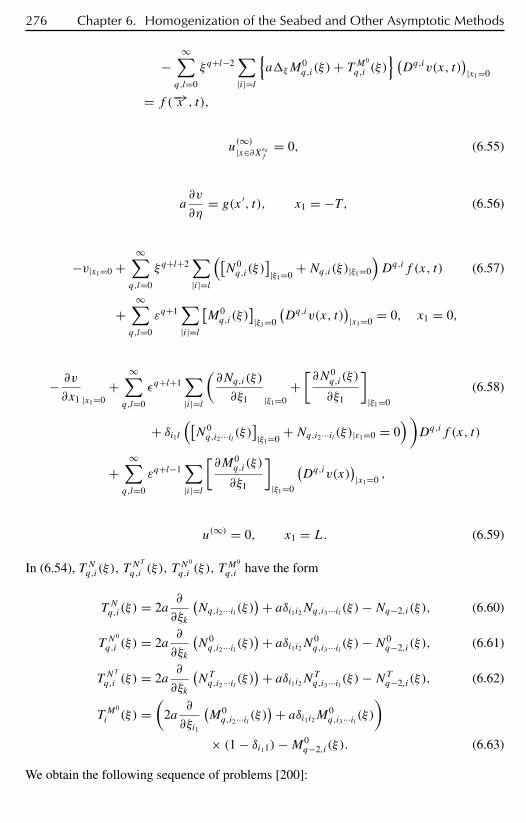
276 Chapter 6. Homogenization of the Seabed and Other Asymptotic Methods
−∞∑q,l=0
ξq+l−2∑|i|=l
aξM
0q,i(ξ)+ T M
0
q,i (ξ) (Dq,iv(x, t)
)|x1=0
= f (−→x , t),
u(∞)|x∈∂Xεεf = 0, (6.55)
a∂v
∂η= g(x ′, t), x1 = −T , (6.56)
−v|x1=0 +∞∑q,l=0
ξq+l+2∑|i|=l
([N0q,i(ξ)
]|ξ1=0
+Nq,i(ξ)|ξ1=0
)Dq,if (x, t) (6.57)
+∞∑q,l=0
εq+1∑|i|=l
[M0q,i(ξ)
]|ξ1=0
(Dq,iv(x, t)
)|x1=0 = 0, x1 = 0,
− ∂v
∂x1 |x1=0+
∞∑q,l=0
εq+l+1∑|i|=l
(∂Nq,i(ξ)
∂ξ1 |ξ1=0+[∂N0
q,i(ξ)
∂ξ1
]|ξ1=0
(6.58)
+ δi1l([N0q,i2···il (ξ )
]|ξ1=0
+Nq,i2···il (ξ )|ε1=0 = 0))Dq,if (x, t)
+∞∑q,l=0
εq+l−1∑|i|=l
[∂M0
q,i(ξ)
∂ξ1
]|ξ1=0
(Dq,iv(x)
)|x1=0 ,
u(∞) = 0, x1 = L. (6.59)
In (6.54), T Nq,i(ξ), TNT
q,i (ξ), TN0
q,i (ξ), TM0
q,i have the form
T Nq,i(ξ) = 2a∂
∂ξk
(Nq,i2···il (ξ )
)+ aδi1i2Nq,i3···il (ξ )−Nq−2,i (ξ), (6.60)
T N0
q,i (ξ) = 2a∂
∂ξk
(N0q,i2···il (ξ )
)+ aδi1i2N0q,i3···il (ξ )−N0
q−2,i (ξ), (6.61)
T NT
q,i (ξ) = 2a∂
∂ξk
(NTq,i2···il (ξ )
)+ aδi1i2NTq,i3···il (ξ )−NTq−2,i (ξ), (6.62)
T M0
i (ξ ) =(
2a∂
∂ξi1
(M0q,i2···il (ξ )
)+ aδi1i2M0q,i3···il (ξ )
)× (1 − δi11)−M0
q−2,i (ξ). (6.63)
We obtain the following sequence of problems [200]:
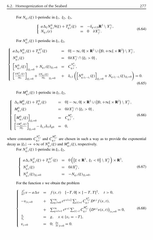
6.2. Homogenization of the Seabed 277
For Nq,i(ξ) 1-periodic in ξ1, ξ2, ξ3,aξN
0q,i9(ξ)+ T Nq,i(ξ) = −δq+l,0R3 \Xε1
f ,
Nq,i(ε) = 0 ∂Xε1f .
(6.64)
For N0q,i(ξ) 1-periodic in ξ1, ξ2,
aξN0q,i(ξ)+ T N0
q,i (ξ) = 0] − ∞, 0[ × R2 ∪ (]0,+∞[ × R2) \Xε1
f ,
N0q,i(ξ) = 0∂Xε1
f ∩ ξ1 > 0 ,[N0q,i(ξ)
]|ξ1=0
+Nq,i(ξ)|ξ1=0 = CN0q,i
q,i ,[∂N0
q,i (ξ)
∂ξ1
]|ξ1=0
+ ∂Nq,i (ξ)
∂ξ1 |ξ1=0+ δi11
([N0q,i2···i1(ξ)
]|ξ1=0
+Nq,i2···i1(ξ)|ξ1=0
)= 0.
(6.65)
ForM0q,i(ξ) 1-periodic in ξ1, ξ2,
ξM0q,i(ξ)+ T 0
q,i(ξ) = 0] − ∞, 0[ × R2 ∪ (]0,+∞[ × R2) \Xε1
f ,
M0q,i(ξ) = 0∂Xε1
f ∩ ξ1 > 0 ,[M0q,i(ξ)
]|ξ1=0
= CM0q,i
q,i ,[∂M0
q,i (ξ)
∂ξ1
]|ξ1=0
− δi11δl1δq0 = 0,
(6.66)
where constants CN0q,i
q,i and CM0q,i
q,i are chosen in such a way as to provide the exponentialdecay as |ξ1| → +∞ of N0
q,i(ξ) andM0q,i(ξ), respectively.
For NTq,i(ξ) 1-periodic in ξ1, ξ2,aεN
Tq,i(ξ)+ T NTq,i (ξ) = 0
(ξ ∈ R3, ξ1 < 0
\Xε1f
)× R2,
NTq,i(ξ) = 0∂Xε1f ,
NTq,i(ξ)|ξ1=0 = −Nq,i(ξ)|ξ1=0.
(6.67)
For the function v we obtain the problem
∂2
∂t2v − av = f (x, t) [−T , 0[ × ] − T , T [2, t > 0,
−v|x1=0 + ∑∞q,l=0 ε
q+l+2 ∑|i|=l CN0q,i
q,i Dq,if (x, t),
+ ∑∞q+l=1 ε
q+l∑|i|−l CM0q,i
q,i
(Dq,iv(x, t)
)|x1=0 = 0,
∂v∂η
= g, x ∈ x1 = −T ,v|t=0 = 0; ∂v
∂t |t=0= 0.
(6.68)
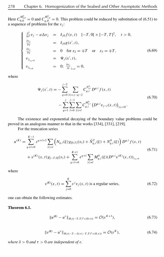
278 Chapter 6. Homogenization of the Seabed and Other Asymptotic Methods
Here CM0
0,∅0,∅ = 0 and C
M01,∅
q,∅ = 0. This problem could be reduced by substitution of (6.51) toa sequence of problems for the vj :
∂2
∂t2vj − avj = δj0f (x, t) [−T , 0[ × [−T , T ]2, t > 0,
∂vj∂η
= δj0g(x′, t),
∂vj∂η
= 0 for x2 = ∓T or x3 = ∓T ,vj|x1=0
= $j(x′, t),
vj|t=0= 0; ∂vj
∂t |t=0= 0,
(6.69)
where
$j(x′, t) = −
j−2∑q=0
∑|i|=j−q−2
CN0q,i
q,i Dq,if (x, t)
−j∑q=1
j−1∑l=0
∑|i|=l
CM0q,i
q,i
(Dq,ivj−l(x, t)
)|x1=0 .
(6.70)
The existence and exponential decaying of the boundary value problems could beproved in an analogous manner to that in the works [334], [331], [219].
For the truncation series
u(K) =K−1∑q+l=0
εq+l+2∑|i|=l
(Nq,i(ξ)χ[0,T ](x1)+ NTq,i(ξ)+N0
q,i(ξ))Dq,if (x, t)
+ v(K)(x, t)χ[−T ,0](x1)+K+1∑q+l=0
εq+l∑|i|=l
M0q,i(ξ)(D
q,iv(K)(x, t))|x1=0
(6.71)
where
v(K)(x, t) =K∑j=0
εjvj (x, t) is a regular series, (6.72)
one can obtain the following estimates.
Theorem 6.1.
‖u(K) − uε‖H1((−T ,T )3×(0,τ )) = O(εK+1), (6.73)
‖v(K) − uε‖H1((−T ,−δ)×(−T ,T )2×(0,τ )) = O(εK), (6.74)
where δ > 0 and τ > 0 are independent of ε.
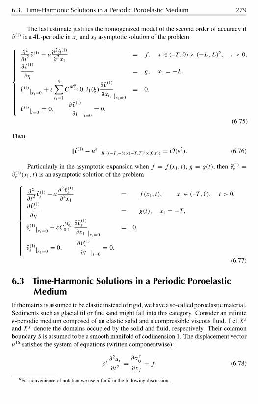
6.3. Time-Harmonic Solutions in a Periodic Poroelastic Medium 279
The last estimate justifies the homogenized model of the second order of accuracy ifv(1) is a 4L-periodic in x2 and x3 asymptotic solution of the problem
∂2
∂t2v(1) − a ∂2v(1)
∂2x1= f, x ∈ (−T , 0)× (−L,L)2, t > 0,
∂v(1)
∂η= g, x1 = −L,
v(1)|x1=0+ ε
3∑i1=1
CM0
0,i1 0, i1(ξ)∂v(1)
∂xi1 |x1=0
= 0,
v(1)|t=0= 0,
∂v(1)
∂t |t=0= 0.
(6.75)
Then
‖v(1) − uε‖H1((−T ,−δ)×(−T ,T )2×(0,τ )) = O(ε2). (6.76)
Particularly in the asymptotic expansion when f = f (x1, t), g = g(t), then v(1)ε =v(1)ε (x1, t) is an asymptotic solution of the problem
∂2
∂t2v(1)ε − a ∂
2v(1)ε∂2x1
= f (x1, t), x1 ∈ (−T , 0), t > 0,
∂v(1)ε
∂η= g(t), x1 = −T ,
v(1)ε |x1=0+ εCM0
0,1
0,1
∂v(1)ε
∂x1 |x1=0
= 0,
v(1)ε |x1=0= 0,
∂v(1)ε
∂t |t=0= 0.
(6.77)
6.3 Time-Harmonic Solutions in a Periodic PoroelasticMedium
If the matrix is assumed to be elastic instead of rigid, we have a so-called poroelastic material.Sediments such as glacial til or fine sand might fall into this category. Consider an infiniteε-periodic medium composed of an elastic solid and a compressible viscous fluid. Let Xs
and Xf denote the domains occupied by the solid and fluid, respectively. Their commonboundary S is assumed to be a smooth manifold of codimension 1. The displacement vectoru16 satisfies the system of equations (written componentwise):
ρs∂2ui
∂t2= ∂σ sij
∂xj+ fi (6.78)
16For convenience of notation we use u for $u in the following discussion.

280 Chapter 6. Homogenization of the Seabed and Other Asymptotic Methods
in Xs , and
ρf∂2ui
∂t2= ∂σ
f
ij
∂xj+ fi (6.79)
in Xf . Moreover, on the interface S, the following transmission conditions hold:
[u] = 0, (6.80)
[σij νj ] = 0,
where νj denote components of the unit normal to S pointing inside ofXs . In the solid part,components of the stress tensor σ s satisfy Hooke’s law:
σ sij = asijklekl(u), ekl(u) = 1
2
(∂uk
∂xl+ ∂ul
∂xk
)(6.81)
with coefficients asijkl ∈ C∞(Xs) satisfying conditions of symmetry and positivity:
asijkl = asjikl = ajilk = asklij ,
k1eij (u)eij (u) ≥ asijkleij (u)ekl(u) ≥ k2eij (u)eij (u). (6.82)
In the fluid part Xf , the stress tensor satisfies the Navier–Stokes law:
σf
ij = −δijP + (λδij δkl + 2µδikδjl)ekl
(∂u
∂t
), (6.83)
where viscosity coefficients µ and λ satisfy
µ > 0,λ
µ> −2
3k2, 0 < k2 < 1. (6.84)
If the displacement is small, we can linearize the equation near the reference state charac-terized by the known reference densities ρs and ρf . The linearized equation of state relatespressure P to the perturbation of density ρ:
P = c2ρ, (6.85)
where c is the speed of sound. Moreover, linearizing the conservation of mass equationpermits the pressure to be eliminated from (6.83):
σf
ij = af
ijklekl(u), (6.86)
where
af
ijkl = −c2ρf δij δkl + (λδij δkl + 2µδikδjl)∂
∂t.
Denote by aijkl the components of symmetric fourth-order tensor equal to asijkl in Xs .
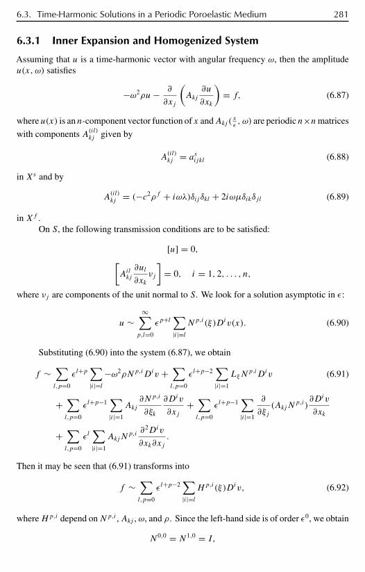
6.3. Time-Harmonic Solutions in a Periodic Poroelastic Medium 281
6.3.1 Inner Expansion and Homogenized System
Assuming that u is a time-harmonic vector with angular frequency ω, then the amplitudeu(x, ω) satisfies
−ω2ρu− ∂
∂xj
(Akj
∂u
∂xk
)= f, (6.87)
where u(x) is an n-component vector function of x andAkj ( xε , ω) are periodic n×nmatrices
with components A(il)kj given by
A(il)kj = asijkl (6.88)
in Xs and by
A(il)kj = (−c2ρf + iωλ)δij δkl + 2iωµδikδjl (6.89)
in Xf .On S, the following transmission conditions are to be satisfied:
[u] = 0,[Ailkj
∂ul
∂xkνj
]= 0, i = 1, 2, . . . , n,
where νj are components of the unit normal to S. We look for a solution asymptotic in ε:
u ∼∞∑
p,l=0
εp+l∑|i|=l
Np,i(ξ)Div(x). (6.90)
Substituting (6.90) into the system (6.87), we obtain
f ∼∑l,p=0
εl+p∑|i|=l
−ω2ρNp,iDiv +∑l,p=0
εl+p−2∑|i|=1
LξNp.iDiv (6.91)
+∑l,p=0
εl+p−1∑|i|=1
Akj∂Np,i
∂ξk
∂Div
∂xj+∑l,p=0
εl+p−1∑|i|=1
∂
∂ξj(AkjN
p,i)∂Div
∂xk
+∑l,p=0
εl∑|i|=1
AkjNp,i ∂
2Div
∂xk∂xj.
Then it may be seen that (6.91) transforms into
f ∼∑l,p=0
εl+p−2∑|i|=l
Hp,i(ξ)Div, (6.92)
whereHp,i depend onNp,i ,Akj , ω, and ρ. Since the left-hand side is of order ε0, we obtain
N0,0 = N1,0 = I,
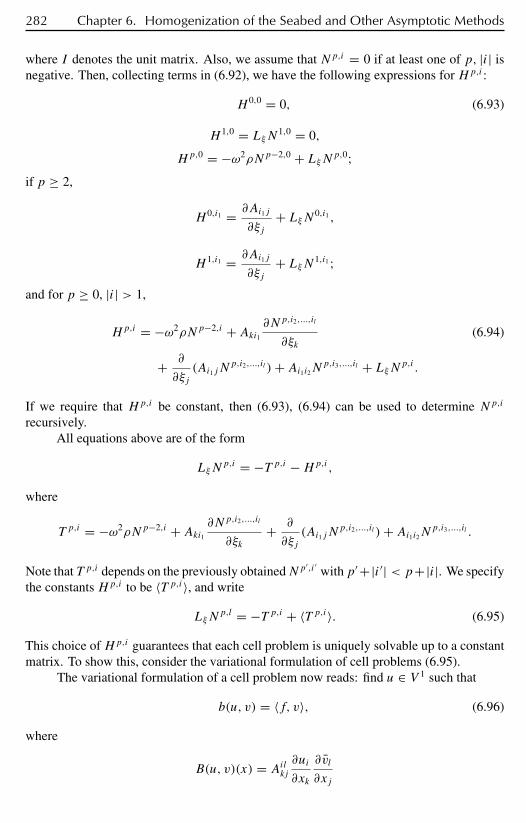
282 Chapter 6. Homogenization of the Seabed and Other Asymptotic Methods
where I denotes the unit matrix. Also, we assume that Np,i = 0 if at least one of p, |i| isnegative. Then, collecting terms in (6.92), we have the following expressions for Hp,i :
H 0,0 = 0, (6.93)
H 1,0 = LξN1,0 = 0,
Hp,0 = −ω2ρNp−2,0 + LξNp,0;if p ≥ 2,
H 0,i1 = ∂Ai1j
∂ξj+ LξN0,i1 ,
H 1,i1 = ∂Ai1j
∂ξj+ LξN1,i1;
and for p ≥ 0, |i| > 1,
Hp,i = −ω2ρNp−2,i + Aki1∂Np,i2,...,il
∂ξk(6.94)
+ ∂
∂ξj(Ai1jN
p,i2,...,il )+ Ai1i2Np,i3,...,il + LξNp,i .
If we require that Hp,i be constant, then (6.93), (6.94) can be used to determine Np,i
recursively.All equations above are of the form
LξNp,i = −T p,i −Hp,i,
where
T p,i = −ω2ρNp−2,i + Aki1∂Np,i2,...,il
∂ξk+ ∂
∂ξj(Ai1jN
p,i2,...,il )+ Ai1i2Np,i3,...,il .
Note that T p,i depends on the previously obtainedNp′,i ′ with p′ +|i ′| < p+|i|. We specify
the constants Hp,i to be 〈T p,i〉, and write
LξNp,l = −T p,i + 〈T p,i〉. (6.95)
This choice of Hp,i guarantees that each cell problem is uniquely solvable up to a constantmatrix. To show this, consider the variational formulation of cell problems (6.95).
The variational formulation of a cell problem now reads: find u ∈ V 1 such that
b(u, v) = 〈f, v〉, (6.96)
where
B(u, v)(x) = Ailkj∂ui
∂xk
∂vl
∂xj
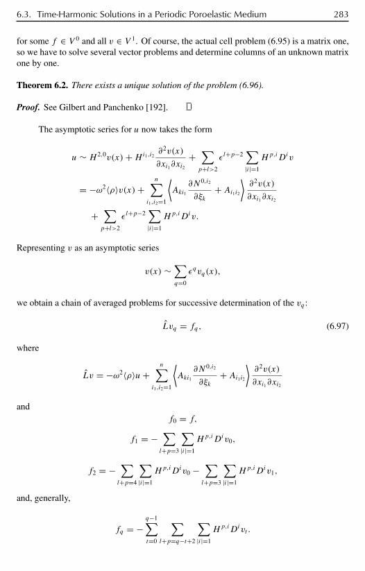
6.3. Time-Harmonic Solutions in a Periodic Poroelastic Medium 283
for some f ∈ V 0 and all v ∈ V 1. Of course, the actual cell problem (6.95) is a matrix one,so we have to solve several vector problems and determine columns of an unknown matrixone by one.
Theorem 6.2. There exists a unique solution of the problem (6.96).
Proof. See Gilbert and Panchenko [192].
The asymptotic series for u now takes the form
u ∼ H 2,0v(x)+Hi1,i2∂2v(x)
∂xi1∂xi2+
∑p+l>2
εl+p−2∑|i|=1
Hp,iDiv
= −ω2〈ρ〉v(x)+n∑
i1,i2=1
⟨Aki1
∂N0,i2
∂ξk+ Ai1i2
⟩∂2v(x)
∂xi1∂xi2
+∑p+l>2
εl+p−2∑|i|=1
Hp,iDiv.
Representing v as an asymptotic series
v(x) ∼∑q=0
εqvq(x),
we obtain a chain of averaged problems for successive determination of the vq :
Lvq = fq, (6.97)
where
Lv = −ω2〈ρ〉u+n∑
i1,i2=1
⟨Aki1
∂N0,i2
∂ξk+ Ai1i2
⟩∂2v(x)
∂xi1∂xi2
andf0 = f,
f1 = −∑l+p=3
∑|i|=1
Hp,iDiv0,
f2 = −∑l+p=4
∑|i|=1
Hp,iDiv0 −∑l+p=3
∑|i|=1
Hp,iDiv1,
and, generally,
fq = −q−1∑t=0
∑l+p=q−t+2
∑|i|=1
Hp,iDivt .

284 Chapter 6. Homogenization of the Seabed and Other Asymptotic Methods
The first equation in the chain (6.97) is the homogenized system:
−ω2ρu+n∑
i1,i2=1
⟨Aki1
∂N0,i2
∂ξk+ Ai1i2
⟩∂2v(x)
∂xi1∂xi2= f. (6.98)
The matrices N0,i2 above are obtained as solutions of the cell problem:
LξN0,i2 = − ∂
∂ξjAi2j (6.99)
satisfying the periodic boundary conditions and the transmission conditions:
[N0,i2 ] = 0
and [Akj
∂Np,i
∂ξkn
]= 0
on the interface hypersurface S.
6.3.2 Interface Matching and Boundary Layers
In the previous section we did not consider boundary conditions, so the construction aboveapplies only locally in R3. To investigate the nature of the changes needed to incorporateboundary effects, consider the following model problem. Suppose that the plane interfacex : x3 = 0 separates two different periodic media. We assume that the equations (6.87)together with the constitutive relations (6.88) with possibly different 1-periodic matricesA±kj are valid in the half-spacesK+ = x : x3 > 0 andK− = x : x3 < 0, respectively. A
particular case of this is acoustics in a two-layer media of the type with homogeneous fluidabove, fluid-saturated sediment below. At this point we prescribe no conditions on u as|x3| → ∞. Our primary interest is to investigate how the presence of the interface affectshomogenization.
For any z = (z1, . . . , z3) ∈ R3, let z denote the vector (z1, z2, 0). In what follows,we use the following notation:
ω(a, b) = x : a < x3 < b,ω(a, b) = x : 0 < xj < 1, j = 1, 2; a < x3 < b,
and
t = x : x3 = t,with t modified accordingly. We also denote
Q = x : xj ∈ (0, 1), j = 1, 2, 3
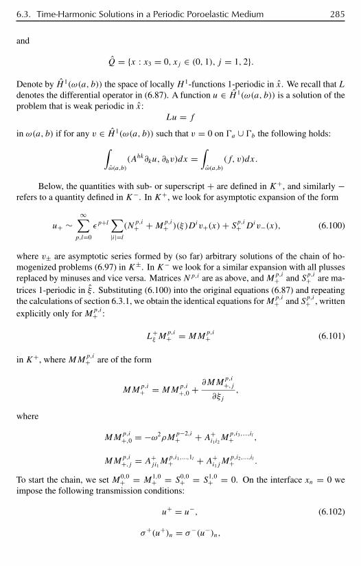
6.3. Time-Harmonic Solutions in a Periodic Poroelastic Medium 285
and
Q = x : x3 = 0, xj ∈ (0, 1), j = 1, 2.
Denote by H 1(ω(a, b)) the space of locally H 1-functions 1-periodic in x. We recall that Ldenotes the differential operator in (6.87). A function u ∈ H 1(ω(a, b)) is a solution of theproblem that is weak periodic in x:
Lu = f
in ω(a, b) if for any v ∈ H 1(ω(a, b)) such that v = 0 on a ∪ b the following holds:∫ω(a,b)
(Ahk∂ku, ∂hv)dx =∫ω(a,b)
(f, v)dx.
Below, the quantities with sub- or superscript + are defined in K+, and similarly −refers to a quantity defined in K−. In K+, we look for asymptotic expansion of the form
u+ ∼∞∑
p,l=0
εp+l∑|i|=l(N
p,i+ +Mp,i
+ )(ξ)Div+(x)+ Sp,i+ Div−(x), (6.100)
where v± are asymptotic series formed by (so far) arbitrary solutions of the chain of ho-mogenized problems (6.97) in K±. In K− we look for a similar expansion with all plussesreplaced by minuses and vice versa. Matrices Np,i are as above, andMp,i
+ and Sp,i+ are ma-trices 1-periodic in ξ . Substituting (6.100) into the original equations (6.87) and repeatingthe calculations of section 6.3.1, we obtain the identical equations forMp,i
+ and Sp,i+ , writtenexplicitly only forMp,i
+ :
L+ξ M
p,i+ = MM
p,i+ (6.101)
in K+, whereMMp,i+ are of the form
MMp,i+ = MM
p,i
+,0 + ∂MMp,i
+,j∂ξj
,
where
MMp,i
+,0 = −ω2ρMp−2,i+ + A+
i1i2Mp,i3,...,il+ ,
MMp,i
+,j = A+ji1Mp,i1,...,1l+ + A+
i1jMp,i2,...,il+ .
To start the chain, we set M0,0+ = M
1,0+ = S
0,0+ = S
1,0+ = 0. On the interface xn = 0 we
impose the following transmission conditions:
u+ = u−, (6.102)
σ+(u+)n = σ−(u−)n,

286 Chapter 6. Homogenization of the Seabed and Other Asymptotic Methods
where
σ±(u±)n = Anj±∂
∂xju±.
These conditions arise due to requirements of continuity of displacements and stresses.Differentiating u± and shifting indices in the sums in the same fashion as in section 6.3.1,we obtain
σ+(u+)N =∞∑
p,l=0
εp+l−1∑|i|=l
[A+nj
∂
∂ξj(N
p,i+ +Mp,i
+ )+ A+ni1(N
p,i2,...,il+
+Mp,i2,...,il+ )
]Div+ +
∞∑p,l=0
εp+l−1∑|i|=l
[A+nj
∂Sp,i+∂ξj
+ A+ni1Sp,i2,...,il+
]Div−,
and a similar expression for σ−(u−)n. Substituting into the second equation in (6.102),collecting terms, and combining with the equations (6.101) we obtain the following trans-mission problems for determination of the pair of matricesMp,i
+ , Sp,i− :
L+ξ M
p,i+ = MM
p,i+ , (6.103)
in K+,
L−ξ S
p,i− = SS
p,i− ,
in K−, with the interface conditions
Np,i+ +Mp,i
+ = Sp,i− + kp,i+ , (6.104)
A+nj
∂
∂ξj(N
p,i+ +Mp,i
+ )+ A+ni1(N
p,i2,...,il+ +Mp,i2,...,il+ ) = A−nj
∂Sp,i−∂ξj
+ A−ni1Sp,i2,...,il− + tp,i+ ,
where kp,i+ , tp,i+ are constant matrices. We look for the solution of this problem in a class
of 1-periodic-in-ξ matrices that decay exponentially as |ξn| → ∞. Similarly, the pairMp,i− , S
p,i+ should be a solution to the problem
L−ξ M
p,i− = MM
p,i− (6.105)
in K−,
L+ξ S
p,i+ = SS
p,i+
in K+,
Np,i− +Mp,i
− = Sp,i+ + kp,i− (6.106)
and
A−nj
∂
∂ξj(N
p,i− +Mp,i
− )+ A−ni1(N
p,i2,...,il− +Mp,i2,...,il− ) = A+nj
∂Sp,i+∂ξj
+ A+ni1Sp,i2,...,il+ + tp,i−

6.3. Time-Harmonic Solutions in a Periodic Poroelastic Medium 287
at the interface. Let us define the operator L to be L+ in K+ and L− in K−. Then theproblems above can be written in common form:
Lu = f in K+ ∪K−, (6.107)
[u] = (x) at xn = 0,
[σ(u)n] = $(x)+ t at xn = 0.
In order to formulate the solvability theorem, we first introduce some definitions.
Definition 6.1. Let u(x, xn) ∈ L2loc be a vector function 1-periodic in x.We say that u has
one-sided exponential decay if the estimate
‖ u ‖L2(Qs)≤ Ce−a|s| (6.108)
holds either for s ∈ Z+ or s ∈ Z− with positive constants C independent of s.If (6.108) holds for all s ∈ Z, we will say that u has two-sided exponential decay.
To describe behavior at infinity we will use the following definition.
Definition 6.2. A vector function u will be called one-sided exponentially stabilizing ifthere exists a constant vector w such that the function u− w satisfies the estimate (6.108)either for s ∈ Z+ or s ∈ Z−. If there is a pair of constant vectors w+, w− such thatone-sided estimates (6.108) hold for both respective differences, we will call u two-sidedexponentially stabilizing to w+, w−.
Theorem 6.3. Suppose that f in (6.107) has two-sided exponential decay. Then thereexist constant vectors t , w+, and w− such that the problem (6.107) has a 1-periodic-in-ξsolution u such that e(u) has two-sided exponential decay and u is two-sided exponentiallystabilizing to w+ and w−.
Moreover,
t =∫K−f (x)dx −
∫K+f (x)dx −
∫Q
$(x)dx. (6.109)
Proof. See [191] for details.
Theorem 6.4. Let s > h > 0 be integers and let u be a periodic-in-x solution of
Lu = 0
in ω(s − h, s + h+ 1). Suppose that P(s − 1, u) = 0. Then∫ω(s,s+1)
|B(u, u)|dx ≤ e−Ah∫ω(s−h,s+h+1)
|B(u, u)|dx, (6.110)
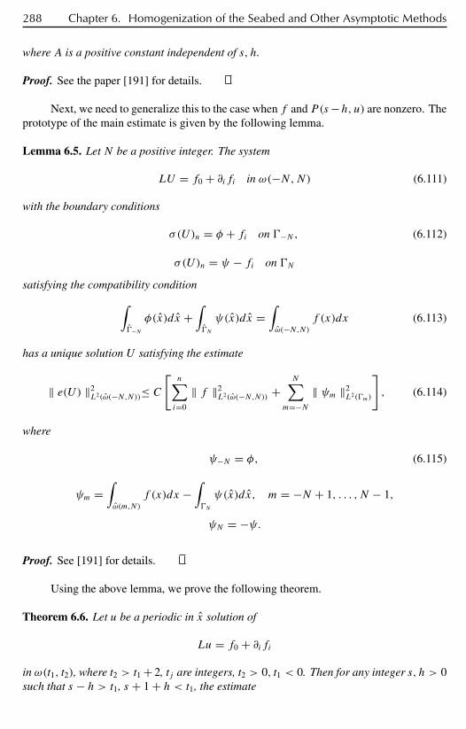
288 Chapter 6. Homogenization of the Seabed and Other Asymptotic Methods
where A is a positive constant independent of s, h.
Proof. See the paper [191] for details.
Next, we need to generalize this to the case when f and P(s−h, u) are nonzero. Theprototype of the main estimate is given by the following lemma.
Lemma 6.5. Let N be a positive integer. The system
LU = f0 + ∂ifi in ω(−N,N) (6.111)
with the boundary conditions
σ(U)n = φ + fi on −N, (6.112)
σ(U)n = ψ − fi on N
satisfying the compatibility condition∫−N
φ(x)dx +∫N
ψ(x)dx =∫ω(−N,N)
f (x)dx (6.113)
has a unique solution U satisfying the estimate
‖ e(U) ‖2L2(ω(−N,N))≤ C
[n∑i=0
‖ f ‖2L2(ω(−N,N)) +
N∑m=−N
‖ ψm ‖2L2(m)
], (6.114)
where
ψ−N = φ, (6.115)
ψm =∫ω(m,N)
f (x)dx −∫N
ψ(x)dx, m = −N + 1, . . . , N − 1,
ψN = −ψ.
Proof. See [191] for details.
Using the above lemma, we prove the following theorem.
Theorem 6.6. Let u be a periodic in x solution of
Lu = f0 + ∂ifiin ω(t1, t2), where t2 > t1 + 2, tj are integers, t2 > 0, t1 < 0. Then for any integer s, h > 0such that s − h > t1, s + 1 + h < t1, the estimate

6.3. Time-Harmonic Solutions in a Periodic Poroelastic Medium 289∫ω(s,s+1)
|e(u)|2dx
≤ C[e−Ah
∫ω(s−h,s+1+h)
|e(u)|2dx +2h+1∑m=0
+∫ω(s−h,s−h+m)
(|f0|2 + (fi, fi))dx
+∣∣∣∣P(s − h, u)+
∫ω(s−h,s−h+m)
f0dx −∫s−h
fidxs
∣∣∣∣2]holds with C independent of s, h. A is a constant from Theorem 6.4.
Proof. See [191] for further details.
As a consequence, we derive the following theorem.
Theorem 6.7. Let fi be a vector function satisfying the inequality
n∑i=0
‖ fi ‖L2(ω(s,s+1)) + ‖ fn ‖L2(s )≤ ce−as, s = 0, 1, 2, . . . , (6.116)
where c, a are positive constants independent of s.Let u be a periodic solution of the system
Lu = f0 + ∂ifiin ω(0,∞) such that P(0, u) = − ∫
ω(0,∞) f0dx + ∫0fn,
‖ e(u) ‖L2(ω(0, 3s+12 ))≤ ce(A−δ)s/2, (6.117)
s = 1, 2, . . . , where c is a constant independent of s, A is a constant from Theorem 6.4,and δ is a constant such that 0 < δ ≤ A.
Then there exist constants C1, C2, a1, a2 independent of s and a constant vector wsuch that
‖ e(u) ‖L2(ω(s,s+1))≤ C1e−a1s , (6.118)
‖ u− w ‖L2(ω(s,s+1))≤ C2e−a2s . (6.119)
Proof. See [191] for further details.
The next result is an existence theorem of the type needed for construction of theboundary layer.
Consider the problem
Lu = f0 + ∂ifi (6.120)
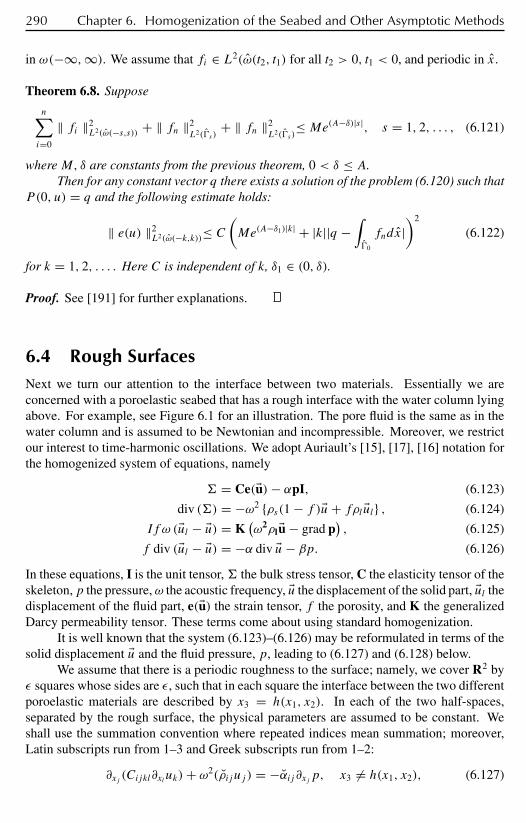
290 Chapter 6. Homogenization of the Seabed and Other Asymptotic Methods
in ω(−∞,∞). We assume that fi ∈ L2(ω(t2, t1) for all t2 > 0, t1 < 0, and periodic in x.
Theorem 6.8. Suppose
n∑i=0
‖ fi ‖2L2(ω(−s,s)) + ‖ fn ‖2
L2(s )+ ‖ fn ‖2
L2(s )≤ Me(A−δ)|s|, s = 1, 2, . . . , (6.121)
whereM, δ are constants from the previous theorem, 0 < δ ≤ A.Then for any constant vector q there exists a solution of the problem (6.120) such that
P(0, u) = q and the following estimate holds:
‖ e(u) ‖2L2(ω(−k,k))≤ C
(Me(A−δ1)|k| + |k||q −
∫0
fndx|)2
(6.122)
for k = 1, 2, . . . . Here C is independent of k, δ1 ∈ (0, δ).
Proof. See [191] for further explanations.
6.4 Rough SurfacesNext we turn our attention to the interface between two materials. Essentially we areconcerned with a poroelastic seabed that has a rough interface with the water column lyingabove. For example, see Figure 6.1 for an illustration. The pore fluid is the same as in thewater column and is assumed to be Newtonian and incompressible. Moreover, we restrictour interest to time-harmonic oscillations. We adopt Auriault’s [15], [17], [16] notation forthe homogenized system of equations, namely
= Ce($u)− αpI, (6.123)
div () = −ω2 ρs(1 − f )$u+ fρl $ul , (6.124)
If ω ($ul − $u) = K(ω2ρl$u − grad p
), (6.125)
f div ($ul − $u) = −α div $u− βp. (6.126)
In these equations, I is the unit tensor, the bulk stress tensor, C the elasticity tensor of theskeleton, p the pressure,ω the acoustic frequency, $u the displacement of the solid part, $ul thedisplacement of the fluid part, e($u) the strain tensor, f the porosity, and K the generalizedDarcy permeability tensor. These terms come about using standard homogenization.
It is well known that the system (6.123)–(6.126) may be reformulated in terms of thesolid displacement $u and the fluid pressure, p, leading to (6.127) and (6.128) below.
We assume that there is a periodic roughness to the surface; namely, we cover R2 byε squares whose sides are ε, such that in each square the interface between the two differentporoelastic materials are described by x3 = h(x1, x2). In each of the two half-spaces,separated by the rough surface, the physical parameters are assumed to be constant. Weshall use the summation convention where repeated indices mean summation; moreover,Latin subscripts run from 1–3 and Greek subscripts run from 1–2:
∂xj (Cijkl∂xl uk)+ ω2(ρij uj ) = −αij ∂xj p, x3 = h(x1, x2), (6.127)
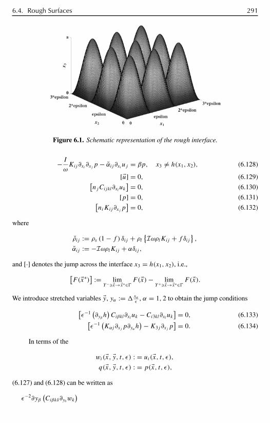
6.4. Rough Surfaces 291
x 3
x1x2
Figure 6.1. Schematic representation of the rough interface.
− IωKij ∂xi ∂xj p − αij ∂xi uj = βp, x3 = h(x1, x2), (6.128)
[$u] = 0, (6.129)[njCijkl∂xl uk
] = 0, (6.130)
[p] = 0, (6.131)[niKij ∂xj p
] = 0, (6.132)
where
ρij := ρs (1 − f ) δij + ρlIωρlKij + f δij
,
αij := −IωρlKij + αδij ,and [·] denotes the jump across the interface x3 = h(x1, x2), i.e.,[
F($x∗)] := lim
Y−-$x→$x∗∈F ($x)− lim
Y+-$x→$x∗∈F ($x).
We introduce stretched variables $y, yα := xαε
, α = 1, 2 to obtain the jump conditions[ε−1
(∂yβh
)Ciβkl∂xl uk − Ci3kl∂xl uk
] = 0, (6.133)[ε−1
(Kαj∂xj p∂yαh
)−K3j ∂xj p] = 0. (6.134)
In terms of the
wi($x, $y, t, ε) : = ui($x, t, ε),q($x, $y, t, ε) : = p($x, t, ε),
(6.127) and (6.128) can be written as
ε−2∂yβ(Ciβkδ∂yδwk
)
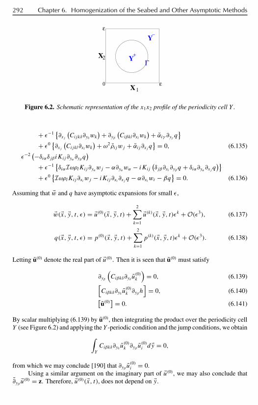
292 Chapter 6. Homogenization of the Seabed and Other Asymptotic Methods
Y+
Y−
Γ
X
X
1
2
ε
0 ε
Figure 6.2. Schematic representation of the x1x2 profile of the periodicity cell Y .
+ ε−1∂xj
(Cijkδ∂yδwk
)+ ∂yβ(Ciβkl∂xlwk
)+ αiγ ∂yγ q
+ ε0∂xj
(Cijkl∂xlwk
)+ ω2ρijwj + αij ∂xj q = 0, (6.135)
ε−2(−δiαδjβiKij ∂yα ∂yβ q)
+ ε−1δiαIωρlKij∂yαwj − α∂yαwα − iKij
(δjβ∂xi ∂yβ q + δiα∂yα ∂xj q
)+ ε0
IωρlKij∂xiwj − iKij ∂xi ∂xj q − α∂xiwi − βq = 0. (6.136)
Assuming that $w and q have asymptotic expansions for small ε,
$w($x, $y, t, ε) = $u(0)($x, $y, t)+2∑k=1
$u(k)($x, $y, t)εk + O(ε3), (6.137)
q($x, $y, t, ε) = p(0)($x, $y, t)+2∑k=1
p(k)($x, $y, t)εk + O(ε3). (6.138)
Letting u(0) denote the real part of $u(0). Then it is seen that u(0) must satisfy
∂yβ
(Ciβkδ∂yδ u
(0)k
)= 0, (6.139)[
Ciβkδ∂yδ u(0)k ∂yβ h
]= 0, (6.140)[
u(0)] = 0. (6.141)
By scalar multiplying (6.139) by u(0), then integrating the product over the periodicity cellY (see Figure 6.2) and applying the Y -periodic condition and the jump conditions, we obtain∫
Y
Ciβkδ∂yδ u(0)k ∂yβ u
(0)i d $y = 0,
from which we may conclude [190] that ∂yβ u(0)i = 0.
Using a similar argument on the imaginary part of $u(0), we may also conclude that∂yβ $u(0) = z. Therefore, $u(0)($x, t), does not depend on $y.
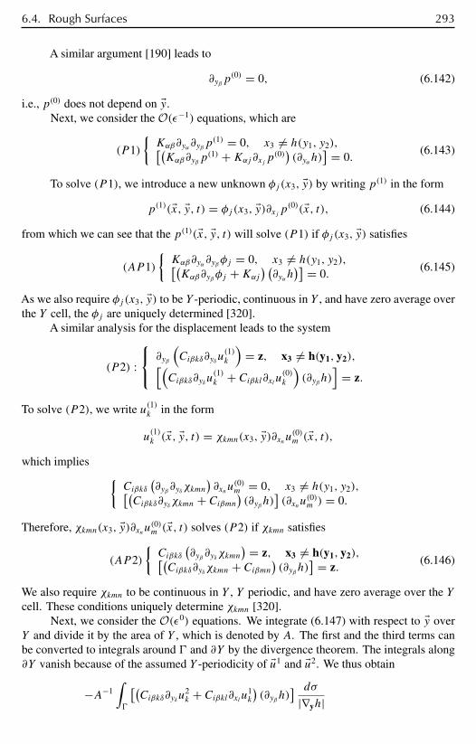
6.4. Rough Surfaces 293
A similar argument [190] leads to
∂yβp(0) = 0, (6.142)
i.e., p(0) does not depend on $y.Next, we consider the O(ε−1) equations, which are
(P1)
Kαβ∂yα∂yβp
(1) = 0, x3 = h(y1, y2),[(Kαβ∂yβp
(1) +Kαj∂xj p(0))(∂yαh)
] = 0.(6.143)
To solve (P1), we introduce a new unknown φj (x3, $y) by writing p(1) in the form
p(1)($x, $y, t) = φj (x3, $y)∂xj p(0)($x, t), (6.144)
from which we can see that the p(1)($x, $y, t) will solve (P1) if φj (x3, $y) satisfies
(AP1)
Kαβ∂yα∂yβφj = 0, x3 = h(y1, y2),[(Kαβ∂yβφj +Kαj
) (∂yαh
)] = 0.(6.145)
As we also require φj (x3, $y) to be Y -periodic, continuous in Y , and have zero average overthe Y cell, the φj are uniquely determined [320].
A similar analysis for the displacement leads to the system
(P2) : ∂yβ
(Ciβkδ∂yδu
(1)k
)= z, x3 = h(y1, y2),[(
Ciβkδ∂yδu(1)k + Ciβkl∂xlu
(0)k
)(∂yβ h)
]= z.
To solve (P2), we write u(1)k in the form
u(1)k ($x, $y, t) = χkmn(x3, $y)∂xnu(0)m ($x, t),
which implies Ciβkδ
(∂yβ ∂yδχkmn
)∂xnu
(0)m = 0, x3 = h(y1, y2),[(
Ciβkδ∂yδχkmn + Ciβmn)(∂yβ h)
](∂xnu
(0)m ) = 0.
Therefore, χkmn(x3, $y)∂xnu(0)m ($x, t) solves (P2) if χkmn satisfies
(AP2)
Ciβkδ
(∂yβ ∂yδχkmn
) = z, x3 = h(y1, y2),[(Ciβkδ∂yδχkmn + Ciβmn
)(∂yβ h)
] = z.(6.146)
We also require χkmn to be continuous in Y , Y periodic, and have zero average over the Ycell. These conditions uniquely determine χkmn [320].
Next, we consider the O(ε0) equations. We integrate (6.147) with respect to $y overY and divide it by the area of Y , which is denoted by A. The first and the third terms canbe converted to integrals around and ∂Y by the divergence theorem. The integrals along∂Y vanish because of the assumed Y -periodicity of $u1 and $u2. We thus obtain
−A−1∫
[(Ciβkδ∂yδu
2k + Ciβkl∂xlu
1k
)(∂yβ h)
] dσ
|∇yh|

294 Chapter 6. Homogenization of the Seabed and Other Asymptotic Methods
+ A−1∫Y
∂xj(Cijkδ∂yδu
1k
)d $y + A−1
∫Y
αiγ ∂yγ p1d $y
+ A−1∫Y
∂xj
(Cijkl∂xlu
(0)k
)d $y + ω2〈ρij 〉u(0)j
+ 〈αij 〉∂xj p(0) = 0, (6.147)
where 〈·〉 is the “averaging operator’’ defined as
〈·〉 := A−1∫Y
·d $y.
By using (6.98), the first integral in (6.147) can be written as
−A−1∫
[Ci3kδ∂yδu
1k + Ci3kl∂xlu
(0)k
] dσ
|∇yh|= −A−1
∫
[Ci3kδ∂yδu
1k
] dσ
|∇yh| − A−1 [Ci3kl] ∂xlu(0)k
∫
dσ
|∇yh|= −A−1
∫
[Ci3kδ∂yδu
1k
] dσ
|∇yh| − A−1 [Ci3kl] ∂xlu(0)k ∂x3A1, (6.148)
where A1 is the area of Y+ [190]. By direct calculation and using the facts that Y+ and Y−are functions of x3 only and $u(0) doesn’t depend on $y, the second integral in (6.147) can beconverted to
A−1(∂xj ∂xnu
(0)m
) ∫Y
Cijkδ∂yδχkmn d $y + A−1(∂xnu
(0)m
) ∫Y
∂x3
(Ci3kδ∂yδχkmn
)d $y. (6.149)
The fourth integral in (6.147) is equal to ∂xj ∂xlu(0)k 〈Cijkl〉 because $u(0) is not a function of $y
and Cijkl are constants in Y+ and Y−. Realizing that 〈Cijkl〉 depends only on x3 and
〈Cijkl〉 = A−1(A1C
+ijkl + (A− A1)C
−ijkl
),
we may further write (∂xj ∂xlu(0)k )〈Cijkl〉 as(
∂xj ∂xlu(0)k
)〈Cijkl〉
= ∂xj
(∂xlu
(0)k 〈Cijkl〉
)+ A−1
(∂x3A1
)[Ci3kl] ∂xlu
(0)k . (6.150)
Finally, we substitute (6.148), (6.149), and (6.150) into (6.147), then replace p1 and u1k by
φj∂xj p(0) and χkmn∂xnu
(0)m , respectively. Note that the last term in (6.148) cancels with the
last term in (6.150). This yields a new equation:
−(A−1
∫
[Ci3kδ∂yδχkmn
] dσ
|∇yh|)∂xnu
(0)m
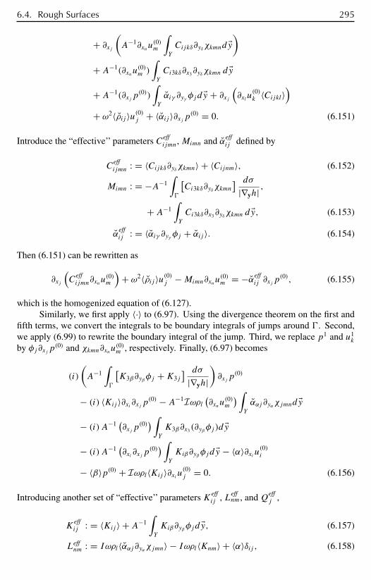
6.4. Rough Surfaces 295
+ ∂xj(A−1∂xnu
(0)m
∫Y
Cijkδ∂yδχkmnd $y)
+ A−1(∂xnu(0)m )
∫Y
Ci3kδ∂x3∂yδχkmn d $y
+ A−1(∂xj p(0))
∫Y
αiγ ∂yγ φjd $y + ∂xj(∂xlu
(0)k 〈Cijkl〉
)+ ω2〈ρij 〉u(0)j + 〈αij 〉∂xj p(0) = 0. (6.151)
Introduce the “effective’’ parameters Ceffijmn,Mimn and αeff
ij defined by
Ceffijmn : = 〈Cijkδ∂yδχkmn〉 + 〈Cijnm〉, (6.152)
Mimn : = −A−1∫
[Ci3kδ∂yδχkmn
] dσ
|∇yh| ,
+ A−1∫Y
Ci3kδ∂x3∂yδχkmn d $y, (6.153)
αeffij : = 〈αiγ ∂yγ φj + αij 〉. (6.154)
Then (6.151) can be rewritten as
∂xj
(C
effijmn∂xnu
(0)m
)+ ω2〈ρij 〉u(0)j −Mimn∂xnu
(0)m = −αeff
ij ∂xj p(0), (6.155)
which is the homogenized equation of (6.127).Similarly, we first apply 〈·〉 to (6.97). Using the divergence theorem on the first and
fifth terms, we convert the integrals to be boundary integrals of jumps around . Second,we apply (6.99) to rewrite the boundary integral of the jump. Third, we replace p1 and u1
k
by φj∂xj p(0) and χkmn∂xnu
(0)m , respectively. Finally, (6.97) becomes
(i)
(A−1
∫
[K3β∂yβφj +K3j
] dσ
|∇yh|)∂xj p
(0)
− (i) 〈Kij 〉∂xi ∂xj p(0) − A−1Iωρl(∂xnu
(0)m
) ∫Y
ααj ∂yαχjmnd $y
− (i) A−1(∂xj p
(0)) ∫
Y
K3β∂x3(∂yβφj )d $y
− (i) A−1(∂xi ∂xj p
(0)) ∫
Y
Kiβ∂yβφjd $y − 〈α〉∂xi u(0)i− 〈β〉p(0) + Iωρl〈Kij 〉∂xi u(0)j = 0. (6.156)
Introducing another set of “effective’’ parameters Keffij , Leff
nm, andQeffj ,
Keffij : = 〈Kij 〉 + A−1
∫Y
Kiβ∂yβφjd $y, (6.157)
Leffnm : = Iωρl〈ααj ∂yαχjmn〉 − Iωρl〈Knm〉 + 〈α〉δij , (6.158)
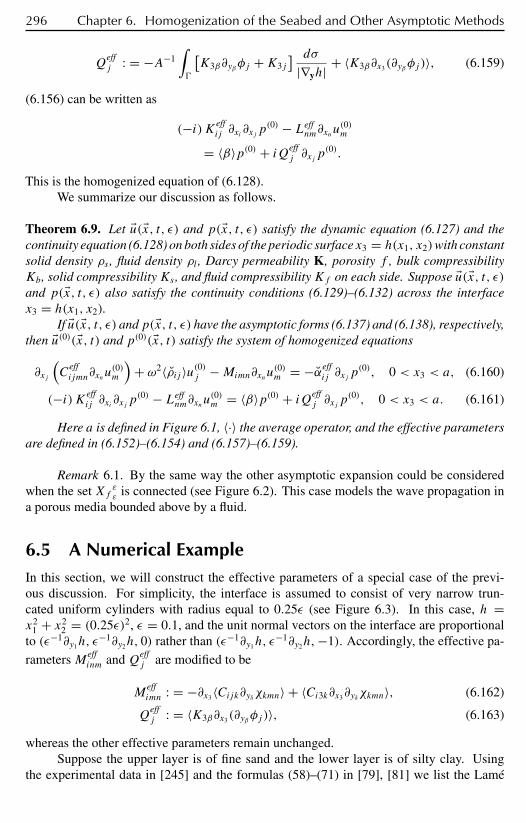
296 Chapter 6. Homogenization of the Seabed and Other Asymptotic Methods
Qeffj : = −A−1
∫
[K3β∂yβφj +K3j
] dσ
|∇yh| + 〈K3β∂x3(∂yβφj )〉, (6.159)
(6.156) can be written as
(−i)Keffij ∂xi ∂xj p
(0) − Leffnm∂xnu
(0)m
= 〈β〉p(0) + iQeffj ∂xj p
(0).
This is the homogenized equation of (6.128).We summarize our discussion as follows.
Theorem 6.9. Let $u($x, t, ε) and p($x, t, ε) satisfy the dynamic equation (6.127) and thecontinuity equation (6.128) on both sides of the periodic surfacex3 = h(x1, x2)with constantsolid density ρs , fluid density ρl , Darcy permeability K, porosity f , bulk compressibilityKb, solid compressibilityKs , and fluid compressibilityKf on each side. Suppose $u($x, t, ε)and p($x, t, ε) also satisfy the continuity conditions (6.129)–(6.132) across the interfacex3 = h(x1, x2).
If $u($x, t, ε) andp($x, t, ε) have the asymptotic forms (6.137) and (6.138), respectively,then $u(0)($x, t) and p(0)($x, t) satisfy the system of homogenized equations
∂xj
(C
effijmn∂xnu
(0)m
)+ ω2〈ρij 〉u(0)j −Mimn∂xnu
(0)m = −αeff
ij ∂xj p(0), 0 < x3 < a, (6.160)
(−i)Keffij ∂xi ∂xj p
(0) − Leffnm∂xnu
(0)m = 〈β〉p(0) + iQeff
j ∂xj p(0), 0 < x3 < a. (6.161)
Here a is defined in Figure 6.1, 〈·〉 the average operator, and the effective parametersare defined in (6.152)–(6.154) and (6.157)–(6.159).
Remark 6.1. By the same way the other asymptotic expansion could be consideredwhen the set Xf εε is connected (see Figure 6.2). This case models the wave propagation ina porous media bounded above by a fluid.
6.5 A Numerical ExampleIn this section, we will construct the effective parameters of a special case of the previ-ous discussion. For simplicity, the interface is assumed to consist of very narrow trun-cated uniform cylinders with radius equal to 0.25ε (see Figure 6.3). In this case, h =x2
1 + x22 = (0.25ε)2, ε = 0.1, and the unit normal vectors on the interface are proportional
to (ε−1∂y1h, ε−1∂y2h, 0) rather than (ε−1∂y1h, ε
−1∂y2h,−1). Accordingly, the effective pa-
rametersMeffinm andQeff
j are modified to be
Meffimn : = −∂x3〈Cijk∂yδχkmn〉 + 〈Ci3k∂x3∂yδχkmn〉, (6.162)
Qeffj : = 〈K3β∂x3(∂yβφj )〉, (6.163)
whereas the other effective parameters remain unchanged.Suppose the upper layer is of fine sand and the lower layer is of silty clay. Using
the experimental data in [245] and the formulas (58)–(71) in [79], [81] we list the Lamé
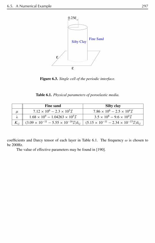
6.5. A Numerical Example 297
ε
ε
Silty ClayFine Sand
0.25ε
Figure 6.3. Single cell of the periodic interface.
Table 6.1. Physical parameters of poroelastic media.
Fine sand Silty clayµ 7.12 × 10⁶ − 2.3 × 10⁵I 7.86 × 10⁶ − 2.5 × 10⁴Iλ 1.68 × 10⁹ − 1.04263 × 10⁵I 3.5 × 10⁸ − 9.6 × 10⁴IKij (3.09 × 10⁻¹¹ − 5.55 × 10⁻¹⁶I)δij (5.15 × 10⁻¹¹ − 2.34 × 10⁻¹⁵I)δij
coefficients and Darcy tensor of each layer in Table 6.1. The frequency ω is chosen tobe 200Hz.
The value of effective parameters may be found in [190].


Bibliography
[1] P. B.Abraham and H. E. Moses. Exact solutions of the one-dimensional acoustic waveequations for several new velocity profiles: Transmission and reflection coefficients.J. Acoustical Soc. Am., 71:1391–1399, 1982.
[2] J. D. Achenbach. Wave Propagation in Elastic Solids. North-Holland, Amsterdam,1976.
[3] K. Aki and P. G. Richards. Quantitative Seismology Theory and Methods. W. H. Free-man and Company, New York, 1980.
[4] A. Alippi and G. B. Cannelli. Proceedings of the Fourth European Conference onUnderwater Acoustics. CNR-IDAC, Rome, 1998.
[5] R. A. Altenburg, N. P. Chotiros, and C. M. Faulkner. Plane-wave analysis of acousticsignals in a sandy sediment. J. Acoustical Soc. Am., 89:165–170, 1990.
[6] D. Ahluwalia and J. Keller. Exact and asymptotic representations of the sound fieldin a stratified ocean. In Wave Propagation and Underwater Acoustics, pages 14–85.Lecture Notes in Physics 70. Springer-Verlag, Berlin, 1977.
[7] T.Angell, D. Colton, andA. Kirsch. The three-dimensional inverse scattering problemfor acoustic waves. J. Differential Equations, 46:46–58, 1982.
[8] T. S. Angell, X. Jiang, and R. E. Kleinman. A distributed source method for inverseacoustic scattering. Inverse Problems, 13:531–545, 1997.
[9] T. S. Angell, R. E. Kleinman, C. Rozier, and D. Lesselier. Uniqueness and CompleteFamilies for an Acoustic Waveguide Problem. Technical report 4, Wave Center,University of Delaware, Newark, 1996.
[10] H. Antoine and P. Cristini. Experimental investigation of the acoustic field in ashallow water waveguide containing an elastic target. In Proceedings of the FourthEuropean Conference on Underwater Acoustics, pages 807–812. CNR-IDAC, Rome,1998.
[11] H. Antoine and P. Cristini. Influence of the presence of an elastic shell in shallowwater: Theoretical and experimental study. Acustica-Acta Acust., 85:24–30, 1999.
299
300 Bibliography
[12] Y. Arnaoudov and G. Dassios. High-frequency asymptotics in inverse scattering byellipsoids. Math. Methods Appl. Sci., 16:1–12, 1993.
[13] R. Au. The Sonar of Dolphins. Springer-Verlag, New York, 1993.
[14] W. W. L. Au and K. Banks. The acoustics of the snapping shrimp synalpheus par-neomeris in Kaneohe Bay. J. Acoustical Soc. Am., 103:41–47, 1998.
[15] J.-L. Auriault. Dynamic behaviour of a porous medium saturated by a newtonianfluid. Internat. J. Eng. Sci., 16:775–785, 1980.
[16] J.-L.Auriault. Poroelastic media. In U. Hornung, editor, Homogenization and PorousMedia, pages 163–182. Springer-Verlag, Berlin, New York, 1997.
[17] J.-L. Auriault, L. Borne, and R. Chambers. Dynamics of a porous saturated media,checking out the generalized law of Darcy. J. Acoustical Soc. Am., 28:1641–1650,1985.
[18] A. V. Badanin and B. P. Belinskii. Oscillations of a liquid in a bounded cavity witha plate on the boundary. Comput. Math. Math. Phys., 33:829–835, 1993.
[19] R. P. Banaugh and W. Goldsmith. Diffraction of steady acoustic waves by surfacesof arbitrary shape, J. Acoustical Soc. Am., 35:1590–1601, 1963.
[20] R. G. Barakat. Transient diffraction of scalar waves by a fixed sphere. J. AcousticalSoc. Am., 32:61–66, 1960.
[21] J. E. Barger. Sonar systems. In M. J. Crocker, editor, Handbook of Acoustics, pages435–455. Wiley, New York, 1998.
[22] F. G. Bass and I. M. Fuks. Wave Scattering from Statistically Rough Surfaces. Perg-amon, Oxford, UK, 1979.
[23] F. Beaumont, M. Garajeu, and A. Wirgin. Scattering of SH-waves by a discontinuityin the material properties and/or by a crack in an infinite plate. Review of Progressin Quantitative NDE, 18A:63–70, 1999.
[24] E. Bécache, P. Joly, and C. Tsogka. An analysis of new mixed finite elements for theapproximation of wave propagation problems. SIAM J. Numer. Anal., 37:1053–1084,2000.
[25] P. Beckmann and A. Spizzichino. The Scattering of Electromagnetic Waves FromRough Surfaces. Pergamon, Oxford, UK, 1963.
[26] J. H. Beebe, S. T. McDaniel, and L. A. Rubano. Shallow-water transmission lossprediction using the Biot sediment model. J. Acoustical Soc. Am., 71:1417–1426,1982.
[27] T. G. Bell. Sonar and submarine detection. Report 545, USN Underwater SoundLaboratory, Harvard University, Cambridge, MA, 1962.
Bibliography 301
[28] A. F. Bennett. Inverse Methods in Physical Oceanography. Cambridge UniversityPress, Cambridge, UK, 1992.
[29] C. L. Bennett and H. Mieras. Time domain integral equation solution for acousticscattering from fluid targets. J. Acoustical Soc. Am., 69:1261–1265, 1981.
[30] J. Benson, N. R. Chapman, and A. Antoniou. Geoacoustic model inversion usingartificial neural networks. Inverse Problems, 16:1627–1640, 2000.
[31] A. P. Berkhoff, J. M. Thijssen, and P. M. van den Berg. Ultrasound wave propagationthrough rough interfaces: Iterative methods. J. Acoustical Soc. Am., 99:1306–1314,1996.
[32] J. Berryman, L. Borcea, G. Papanicolaou, and C. Tsogka. Statistically stable ultrasonicimaging in random media. J. Acoustical Soc. Am., 112:1509–1522, 2002.
[33] J. Berryman, L. Borcea, G. Papanicolaou, and C. Tsogka. Imaging methods in ran-dom media. In A. Wirgin, editor, Acoustics, Mechanics, and the Related Topics ofMathematical Analysis, pages 14–20. World Scientific, Singapore, 2003.
[34] J. G. Berryman. Single-scattering approximations for coefficients in Biot’s equationsof poroelasticity. J. Acoustical Soc. Am., 91:551–571, 1992.
[35] M. A. Biot. General theory of three-dimensional consolidation. J. Applied Physics,12:155–164, February 1941.
[36] M. A. Biot. Theory of propagation of elastic waves in a fluid-saturated porous solid:I. Lower frequency range. J. Acoustical Soc. Am., 28:168–178, 179–191, 1956.
[37] M. A. Biot and D. G. Willis. The elastic coefficients of the theory of consolidation.J. Appl. Mech., 24:594–601, 1957.
[38] M. A. Biot. Theory of propagation of elastic waves in a fluid-saturated porous solid.II. Higher frequency range. J. Acoustical Soc. Am., 28:179–191, 1956.
[39] M. A. Biot. Generalized theory of acoustic propagation in porous dissipative media.J. Acoustical Soc. Am., 34:1254–1264, 1962.
[40] M. A. Biot. Mechanics of deformation and acoustic propagation in porous media. J.Appl. Phys., 33:1482–1498, 1962.
[41] T. G. Birdsall and K. Metzger. Factor inverse matched filtering. J. Acoustical Soc.Am., 79:91–99, 1986.
[42] G. C. Bishop and J. Smith. Scattering from an elastic shell and a rough fluid-elasticinterface: Theory. J. Acoustical Soc. Am., 101:767–788, 1997.
[43] G. C. Bishop and J. Smith. Scattering from rigid and soft targets near a planarboundary: Numerical results. J. Acoustical Soc. Am., 105:130–143, 1999.
[44] L. Bjorno and S. Sun. Use of the Kirchhoff approximation in scattering from elastic,rough surfaces. Acoustical Phys., 41:637–648, 1995.
302 Bibliography
[45] M. Bocly, M. Lambert, C. Rozier, and D. Lesselier. Optimal contour reconstructionof a sound-hard obstacle in a shallow water acoustic waveguide. In A. Alippi and G.B. Cannelli, editors, Proceedings of the Fourth European Conference on UnderwaterAcoustics, pages 643–648. CNR-IDAC, Rome, 1998.
[46] R. Bohbot, D. Lesselier, and W. Tabbara. Evaluation de diverses méthodes de diag-nostic acoustique d’un fond marin stratifié. J. Phys. Coll., 51 supp. au no. 2:997–1000,1990.
[47] J. C. Bolomey and A. Wirgin. Numerical comparison of the Green’s function and thewaterman and Rayleigh theories of scattering from a cylinder with arbitrary cross-section. Proc. IEEE, 121:794–804, 1974.
[48] M. Bonnet. BIE and material differentiation applied to the formulation of obstacleinverse problems. Engrg. Anal. Bound. Elem., 15:121–136, 1995.
[49] M. Bonnet. Boundary Integral Equation Methods for Solids and Fluids. Wiley,Chichester, UK, 1995.
[50] L. Borcea, G. C. Papanicolaou, C. Tsogka, and J. G. Berryman. Imaging and timereversal in random media. Inverse Problems, 18:1247–1279, 2002.
[51] M. Bouvet. Traitements des signaux pour les systèmes sonar. Masson, Paris, 1992.
[52] C. A. Boyles. Acoustic Waveguides. Wiley, New York, 1984.
[53] L. Brekhovskikh andV. Lysanov. Fundamentals of OceanAcoustics. Springer-Verlag,Berlin, 1982.
[54] L. M. Brekhovskikh. Waves in Layered Media. 2nd ed. Academic Press, New York,1980.
[55] L. M. Brekhovskikh and O. A. Godin. Acoustics of Layered Media. Springer-Verlag,Berlin, 1990.
[56] D. Brill, G. C. Gaunaurd, and H. Uberall. Mechanical eigenfrequencies of axisym-metric fluid objects: Acoustic spectroscopy. Acustica, 53:11–18, 1983.
[57] M. G. Brown. Linearized travel time, intensity, and waveform inversions in the oceansound channel—a comparison. J. Acoustical Soc. Am., 75:1451–1461, 1984.
[58] O. Bruno and F. Reitich. Numerical solution of diffraction problems: A method ofvariation of boundaries. J. Opt. Soc. Amer., 10:1168–1175, 1993.
[59] O. Bruno and F. Reitich. Numerical solution of diffraction problems: A methodof variation of boundaries. ii finitely conducting gratings, padé approximants, andsingularities. J. Opt. Soc. Amer., 10:2307–2316, 1993.
[60] O. Bruno and F. Reitich. Numerical solution of diffraction problems: A method ofvariation of boundaries. III. Doubly periodic gratings. J. Opt. Soc. Amer., 10:2551–2562, 1993.

Bibliography 303
[61] O. Bruno and F. Reitich. Approximation of analytic functions: A method of enhancedconvergence. Math. Comput., 63:195–215, 1994.
[62] O. P. Bruno and F. Reitich. Boundary-variation solutions for bounded-obstacle scat-tering problems in three dimensions. J. Acoustical Soc. Am., 104:2579–2583, 1998.
[63] B.A. Brunson and R. K. Johnson. Laboratory measuements of shear wave attenuationin saturated sand. J. Acoustical Soc. Am., 68:1371–1375, 1980.
[64] G. M. Bryan and R. D. Stoll. The dynamic shear modulus of marine sediments. J.Acoustical Soc. Am., 83:2159–2164, 1988.
[65] J. Buchanan and R. Gilbert. Transmission loss in the far field over a seabed with rigidsubstrata assuming the Biot sediment model. J. Computational Acoust., 4:29–54,1996.
[66] J. Buchanan, R. Gilbert, and A. Wirgin. Finding an inclusion in a shallow ocean usinga canonical domain method. In A. Alippi and G. B. Canneli, editors, Proceedings ofthe Fourth European Conference on Underwater Acoustics, pages 389–394. CNR-IDAC, Rome, 1998.
[67] J. Buchanan, R. P. Gilbert, A. Wirgin, and Y. Xu. The unidentified object problemin a shallow ocean with a fluid-like sediment layer overlying a rigid seabed. Appl.Anal., 73:5–17, 1999.
[68] J. L. Buchanan, R. P. Gilbert, and M. Ou. Implementation of the method of variationof boundaries for three-dimensional objects in a waveguide. In Mathematical andNumerical Aspects of Wave Propogation (Santiago de Compostela, 2000), pages482–488. SIAM, Philadelphia, 2000.
[69] J. L. Buchanan, R. P. Gilbert, and A. Wirgin. Finding an inclusion in a shallow oceanusing the ICBA method. Appl. Anal., 71:347–378, 1999.
[70] J. L. Buchanan, R. P. Gilbert, and A. Wirgin. Implementation of the ICBA methodfor solids of revolution. In Problemi Atuali dell’Analisi e della Fisica Matematica.Aracne, Rome, 1999.
[71] J. L. Buchanan, R. P. Gilbert, A. Wirgin, and Y. Xu. Identification, by the canonicaldomain method, of the size shape and depth of a soft body of revolution locatedwithin an acoustic waveguide. Inverse Problems, 16:1709–1726, 2000.
[72] J. L. Buchanan, R. P. Gilbert, A. Wirgin, and Yongzhi Xu. Identification by theintersecting canonical domain method of the size, shape and depth of a soft body ofrevolution located within an acoustic waveguide. Report LMA, 11/98-2. 1998.
[73] J. L. Buchanan, P. Cristini, R. P. Gilbert, A. Wirgin, and Yongzhi Xu. Propagation inan acoustic waveguide containing a soft body of revolution. Report PI/LMA, 11/98-4.1998.
304 Bibliography
[74] J. L. Buchanan, R. P. Gilbert, A. Wirgin., and Y. Xu. Depth sounding: An illustrationof some of the pitfalls of inverse scattering problems. Math. Comput. Modelling,35:1315–1354, 2002.
[75] J. L. Buchanan and R. P. Gilbert. Transmission loss in the far field over a seabedwith rigid substrate assuming the Biot sediment model. J. Computational Acoust.,4:29–54, 1996.
[76] J. L. Buchanan and R. P. Gilbert. Transition loss in the farfield for an ocean with aBiot sediment over an elastic substrate. ZAMM, 77:121–135, 1997.
[77] J. L. Buchanan and R. P. Gilbert. Transmission loss in the far field over a one-layerseabed assuming the Biot sediment model. ZAMM, 77:121–135, 1997.
[78] J. L. Buchanan and R. P. Gilbert. Comparison of the solution to a problem inocean acoustics by parabolic approximation with the exact solution obtained fromthe residue calculus. In Generalized Analytic Functions. Kluwer, Dordrecht, theNetherlands, 1998.
[79] J. L. Buchanan and R. P. Gilbert. Determination of the coefficients of an elasticseabed. Appl. Anal., 65:75–86, 1998.
[80] J. L. Buchanan and R. P. Gilbert. Simplex-based algorithms for determining thecoefficients of an elastic seabed. In K. Hackl, K. Florian, and W. Tutschke, editors,Analytic Functions. Kluwer, Dordrecht, the Netherlands, 1998.
[81] J. L. Buchanan and R. P. Gilbert. Transmission loss in a stratified ocean over aporoelastic seabed. In H. Begehr, R. P. Gilbert, and G.-C. Wen, editors, Proceedingsof the First ISAAC Conference. Kluwer, Dordrecht, the Netherlands, 1998.
[82] J. L. Buchanan and R. P. Gilbert. Transmission loss over a two-layer seabed. Internat.J. Solids Structures, 35:4779–4801, 1998.
[83] J. L. Buchanan, R. P. Gilbert, Z. Lin, and Y. Xu. Direct and inverse problems in oceanacoustics. Nonlinear Analysis, 30:1535–1546, 1996.
[84] J. L. Buchanan, R. P. Gilbert, and Y. Xu. Green’s function representation for acousticpressure over a poroelastic seabed. Appl. Anal., 65:57–68, 1997.
[85] H. P. Bucker. Use of calculated wave field and matched field detection to locate soundsource in shallow water. J. Acoustical Soc. Am., 59:368–373, 1976.
[86] M. Buckingham, J. Potter, and C. Epifanio. L’imagerie acoustique. Pour la Science,No. hors série: Le monde des sons, Juillet/Août:54–57, 2001.
[87] M. J. Buckingham. Seismic wave propagation in rocks and marine sediments: Anew theoretical approach. In A. Alippi and G. B. Cannelli, editors, Proceedings ofthe Fourth European Conference on Underwater Acoustics, pages 299–300. CNR-IDAC, Rome, 1998.
Bibliography 305
[88] M. J. Buckingham. Theory of compressional and shear waves in fluid-like marinesediments. J. Acoustical Soc. Am., 103:288–299, 1998.
[89] M. J. Buckingham. Theory of acoustic propagation around a conical seamount. J.Acoustical Soc. Am., 80:265–277, 1986.
[90] H. D. Bui. Introduction aux problèmes inverses en mécanique des matériaux. Ey-rolles, Paris, 1993.
[91] R. Burridge and J. B. Keller. Poroelasticity equations derived from micro-structure.J. Acoustical Soc. Am., 70:1140–1146, 1981.
[92] A. Burton and G. Miller. The application of integral equations methods to the nu-merical solution of some exterior boundary value problems. Proc. Roy. Soc. LondonSer. A, 323:201–210, 1971.
[93] A. J. Burton and G. F. Miller. The application of integral equation methods to thenumerical solutions of some exterior boundary-value problems. Proc. Roy. Soc.London Ser. A, 323:201–210, 1971.
[94] A. Caiti, J.-P. Hermand, S. Jesus, and M. Porter. Experimental Acoustic InversionMethods for Exploration of the Shallow Water Environment. Kluwer, Amsterdam,2000.
[95] J. M. Carcione. Wave Fields in Real Media: Wave Propagation in Anisotropic,Anelastic and Porous Media. Pergamon-Elsevier, Oxford, UK, 2001.
[96] P. Carrion. Reflection tomography in underwater acoustics. J. Acoustical Soc. Am.,97:1318–1321, 1995.
[97] P. Carrion and G. Boehm. Tomographic imaging of opaque and low-contrast objectsin range-independent waveguides. J. Acoustical Soc. Am., 91:1440–1446, 1992.
[98] R. Carroll. Transmutation and Operator Differential Equations. North-Holland,Amsterdam, 1979.
[99] R. Carroll. The Bergman-Gilbert opearator as a transmutation. C. R. Math. Rep.Acad. Sci. Canada, 4:267–269, 1982.
[100] E. L. Carstensen and L. L. Foldy. Propagation of sound through a liquid containingbubbles. J. Acoustical Soc. Am., 19:481–501, 1947.
[101] K. Chadan and P. C. Sabatier. Inverse Problems in Quantum Scattering Theory.Springer-Verlag, Berlin, 1989.
[102] J. R. Chamuel. An explanation for the anomalous ultrasonic slow wave in underwatersand. IEEE Trans. Ultrason. Ferroel. Freq. Control, 45:1441–1443, 1998.
[103] R. Chapman and A. Tolstoy. Special issue: Benchmarking geoacoustic inversionmethods. J. Computational Acoust., 6(1 & 2), 1998.
306 Bibliography
[104] A. Charalambopoulos, G. Dassios, and P. Ergatis. A small axisymmetric obstacle inthe presence of an underwater point-source field. J. Computational Acoust., 5:243–263, 1997.
[105] G. Chavent and P. C. Sabatier. Inverse Problems of Wave Propagation and Diffraction.Springer-Verlag, Berlin, 1997.
[106] C. Chen and M.-K. Kuo. Computing and modeling in underwater acoustics, seis-mology and wave propagation. J. Computational Acoust., 9:395–703, 2001.
[107] G. Chen and J. Zhou. Boundary Element Methods. Academic Press, New York, 1992.
[108] J. M. Chesneaux and A. Wirgin. Reflection from a corrugated surface revisited. J.Acoustical Soc. Am., 96:1116–1129, 1994.
[109] P. Chevret, N. Gache, and V. Zimpfer. Target classification near complex bound-aries. In A. Alippi and G. B. Cannelli, editors, Proceedings of the Fourth EuropeanConference on Underwater Acoustics, pages 825–830. CNR-IDAC, Rome, 1998.
[110] W. C. Chew. Waves and fields in Inhomogeneous Media. IEEE Press, New York,1995.
[111] N. P. Chotiros. Biot model of sound propagation in water-saturated sand. J. AcousticalSoc. Am., 97:199–214, 1995.
[112] N. P. Chotiros. Biot model of sound propagation in water-saturated sand. J. AcousticalSoc. Am., 97:199–214, 1995.
[113] N. P. Chotiros. Response to: “Comments on Biot model of sound propagation inwater-saturated sand [J.Acoustical Soc.Am. 103, 2723–2725 (1998)], ’’ J.AcousticalSoc. Am., 103:2726–2729, 1998.
[114] D. Chu, T. K Stanton, and P. H. Wiebe. Model-based acoustic characterization andclassification of irregular-shaped targets: Application to fisheries and zooplanktonacoustics. J. Acoustical Soc. Am., 112:2307–2314, 2002.
[115] C. Collet, P. Thourel, M. Mignotte, P. Perez, and P. Bouthemy. Segmentation markovi-enne hierarchique multimodèle d’images sonar haute résolution. Traitement du Sig-nal, 15:231–249, 1998.
[116] M. D. Collins. Higher-order and elastic parabolic equations for wave propagationin the ocean. In D. Lee, A. Cakmak, and R. Vichnevetsky, editors, ComputationalAcoustics, Volume 3, pages 167–184. Elsevier, Amsterdam, 1990.
[117] M. D. Collins. Higher order Padé approximations for accurate and stable elasticparabolic equations with application to interface wave propagation. J. AcousticalSoc. Am., 89:1050–1057, 1991.
[118] M. D. Collins. Topics in ocean acoustic inverse problems. In G. Chavent, G. Papan-icolaou, P. Sacks, and W. Symes, editors, Inverse Problems in Wave Propagation,pages 85–104. Springer-Verlag, New York, 1997.

Bibliography 307
[119] M. D. Collins and W. A. Kuperman. Inverse problems in ocean acoustics. InverseProblems, 10:1023–1040, 1994.
[120] M. D. Collins and W. L. Siegmann. Parabolic equation techniques for wave prop-agation. In J. A. de Santo, editor, Mathematical and Numerical Aspects of WavePropagation, pages 3–11. SIAM, Philadelphia, 1998.
[121] D. Colton, J. Coyle, and P. Monk. Recent developments in inverse acoustic scatteringtheory. SIAM Review, 42:369–414, 2000.
[122] D. Colton, R. Ewing, and W. Rundell, editors. Inverse Problems in Partial DifferentialEquations. SIAM, Philadelphia, 1990.
[123] D. Colton and A. Kirsch. Dense sets and far field patterns in acoustic wave propaga-tion. SIAM J. Math. Anal., 15:996–1006, 1984.
[124] D. Colton and A. Kirsch. A simple method for solving inverse scattering problemsin the resonance region. Inverse Problems, 12:383–393, 1996.
[125] D. Colton and R. Kress. Integral Equation Methods in Scattering Theory. Wiley,New York, 1983.
[126] D. Colton and R. Kress. Inverse Acoustic and Electromagnetic Scattering Theory.Springer-Verlag, Berlin, 1993.
[127] D. Colton and P. Monk. A novel method for solving the inverse scattering problemfor time-harmonic acoustic waves in the resonance region. SIAM J. Appl. Math.,45:1039–1053, 1985.
[128] D. Colton and P. Monk. A novel method for solving the inverse scattering problemfor time-harmonic acoustic waves in the resonance region: II. SIAM J. Appl. Math.,46:506–523, 1986.
[129] D. Colton, M. Piana, and R. Potthast. A simple method using Morozov’s discrepancyprinciple for solving inverse scattering problems. Inverse Problems, 13:1477–1493,1997.
[130] J. P. Corones, G. Kristensson, P. Nelson, and D. L. Seth. Invariant Imbedding andInverse Problems. SIAM, Philadelphia, 1992.
[131] L. Couchman, D. N. Ghosh Roy, and A. G. Ramm. Inversion of low-frequencysubsurface data in a finite-depth ocean. Appl. Math. Lett., 7:11–14, 1994.
[132] G. B. Crawford, R. J. Lataitis, and S. F. Clifford. Remote sensing of ocean flows byspatial filtering of acoustic scintillations theory. J. Acoustical Soc. Am., 88:442–454,1990.
[133] P. Cristini. Quelques caractéristiques de la propagation des ondes acoustiques en eaupeu profonde en présence d’un fond stratifié. Acustica-Acta Acustica, 82:260–267,1996.
308 Bibliography
[134] P. Cristini. A Short Guide to KrakenZ, Publications du LMA 150. LMA/CNRS,Marseille, France, 1998.
[135] P. Cristini and A. Wirgin. Identification of the size, proportions and location of a softbody of revolution in a shallow-water waveguide. Inverse Problems, 16:1727–1740,2000.
[136] M. J. Crocker. Part IV: Underwater sound. In Encyclopedia of Acoustics, pages373–618. Wiley, New York, 1997.
[137] L. J. Cutrona. Comparison of sonar system performance achievable using synthetic-aperture techniques with the performance achievable by more conventional means.J. Acoustical Soc. Am., 58:336–348, 1975.
[138] D. K. Dacol. The Kirchhoff approximation for acoustic scattering from a roughfluid-elastic solid interface. J. Acoustical Soc. Am., 88:978–983, 1990.
[139] G. Dassios. Energy functionals in scattering theory and inversion of low frequencymoments. In A. Wirgin, editor, Wavefield Inversion, pages 1–58. Springer-Verlag,Wien, 1999.
[140] G. Dassios and R. J. Lucas. Inverse scattering for the penetrable ellipsoid and ellip-soidal boss. J. Acoustical Soc. Am., 99:1877–1882, 1996.
[141] T. W. Dawson. Acoustic scattering in a three-dimensional oceanic waveguide usingboundary integral methods. J. Acoustical Soc. Am., 90:2609–2622, 1991.
[142] T. W. Dawson and J. A. Fawcett. A boundary integral equation method for acousticscattering in a waveguide with nonplanar surfaces. J. Acoustical Soc. Am., 87:1110–1125, 1990.
[143] G. Degrande, G. de Roeck, and P. van den Broeck. Wave propagation in layered dry,saturated and unsaturated poroelastic media. Internat. J. Solids Structures, 35:4753–4778, 1998.
[144] S. Delamare. Une amélioration de la tomographie ultrasonore en réflexion. C. R.Acad. Sci. Paris Ser. IIb, 327:475–480, 1999.
[145] S. Delamare, J.-P. Lefebvre, and A. Wirgin. Ghosts in Born images of a layer probedby acoustic waves. Ultrasonics, 37:633–643, 2000.
[146] J. A. DeSanto. Scalar Wave Theory. Springer-Verlag, Berlin, 1992.
[147] Y. Desaubies, A. Tarantola, and J. Zinn-Justin. Oceanographic and GeophysicalTomography. North-Holland, Amsterdam, 1990.
[148] A. Doicu, Y. Eremin, and T. Wriedt. Acoustic and Electromagnetic Scattering AnalysisUsing Discrete Sources. Academic Press, San Diego, 2000.
[149] S. E. Dosso. Benchmarking range-dependent propagation modeling in matched-fieldinversion. J. Computational Acoust., 10:231–242, 2002.
Bibliography 309
[150] B. Duchêne and W. Tabbara. Characterization of a buried cylindrical object from itsscattered field. IEEE Trans. Sonics Ultrason., 31:658–663, 1984.
[151] R. Duraiswami, S. Prabhukumar, and L. Chahine. Bubble counting using an inverseacoustic scattering method. J. Acoustical Soc. Am., 104:2699–2717, 1998.
[152] M. D. Duston, R. P. Gilbert, and D. H. Wood. Direct generation of normal modes bytransmutation theory. In Computational Acoustics and Wave Propagation, Volume 2.North-Holland, Groningen, the Netherlands, 1988.
[153] M. D. Duston, R. P. Gilbert, and D. H. Wood. A wave propagation computationtechnique using function theoretic representation. In Numerical Mathematics andApplications, pages 281–288. North-Holland, New York, 1986.
[154] J. Dybedal. A high resolution sonar for sea-bed imaging. Ultrasonics, 24:71–76,1985.
[155] S. L. Edelstein. Asymptotic behavior of the modes of a smoothly irregular waveguidewith permeable boundaries. Soviet Phys. Acoustical, 36:193–195, 1990.
[156] H. E. Edgerton. Sonar Images. Prentice-Hall, Englewood Cliffs, NJ, 1986.
[157] J. E. Ehrenberg, T. E. Ewart, and R. D Morris. Signal-processing techniques forresolving individual pulses in a multipath environment. J. Acoustical Soc. Am.,63:1801–1808, 1978.
[158] A. El Badia. Coefficient identification in a parabolic equation from input sourcesand partial boundary measurements. In J. A. de Santo, editor, Mathematical andNumerical Aspects of Wave Propagation, pages 532–534. SIAM, Philadelphia, 1998.
[159] A. C. Eringen. Mechanics of Continua. Wiley, New York, 1967.
[160] R. B. Evans. A coupled mode solution for acoustic propagation in a waveguide withstepwise depth variations of a penetrable bottom. J. Acoustical Soc. Am., 74:188–195,1983.
[161] R. B. Evans and K. E. Gilbert. The periodic extension of stepwise coupled modes.J. Acoustical Soc. Am., 77:963–988, 1985.
[162] J. A. Fawcett. The computation of the scattered pressure field from a cylinder em-bedded between two half-spaces with different densities. J. Acoustical Soc. Am.,99:2435–2438, 1996.
[163] J. A. Fawcett. A plane-wave decomposition method for modeling scattering fromobjects and bathymetry in a waveguide. J. Acoustical Soc. Am., 100:183–192, 1996.
[164] J. A. Fawcett. Modeling acousto-elastic waveguide/object scattering with theRayleigh hypothesis. J. Acoustical Soc. Am., 106:164–168, 1999.
[165] J. A. Fawcett. Modeling of scattering by partially buried elastic cylinders. J. Acous-tical Soc. Am., 105:2628–2633, 1999.

310 Bibliography
[166] J. A. Fawcett, M. L. Yeremy, and N. R. Chapman. Matched-field source localizationin a range-dependent environment. J. Acoustical Soc. Am., 99:272–282, 1996.
[167] J.A. Fawcett. Coupled-mode modeling of acoustic scattering from three-dimensional,axisymmetric objects. J. Acoustical Soc. Am., 102:3387–3393, 1997.
[168] J. A. Fawcett, W. L. J. Fox, and A. Maguer. Modeling of scattering by objects on theseabed. J. Acoustical Soc. Am., 104:3296–3304, 1998.
[169] N. R. Feuillade and M. F. Werby. Resonant multiple scattering from two deformedwater-entrained air bubbles. Acoust. Lett., 18:19–24, 1994.
[170] P. J. T. Filippi, D. Habault, J.-P. Lefebvre, and A. Bergassoli. Acoustics: BasicPhysics, Theory and Methods. Academic Press, San Diego, 1999.
[171] M. Fink, W. A. Kuperman, J. P. Montagner, and A. Tourin. Imaging of ComplexMedia with Acoustic and Seismic Waves. Springer-Verlag, Berlin, 2002.
[172] M. Fink and C. Prada. Acoustic time-reversal mirrors. Inverse Problems, 17:R1–R38,2001.
[173] L. Fishman. Exact, uniform asymptotic, and numerical constructions of Helmholtzoperator symbols. In J. A. de Santo, editor, Mathematical and Numerical Aspects ofWave Propagation, pages 259–263. SIAM, Philadelphia, 1998.
[174] L. L. Foldy. The multiple scattering of waves. Physical Rev., 67:107–119, 1945.
[175] L. Frank. Singular Perturbations in Elasticity Theory. North-Holland, Groningen,the Netherlands, 1999.
[176] A. Freedman. The high frequency echo structure of some simple body shapes. Acus-tica, 12:63–70, 1962.
[177] J. R. Fricke. Acoustic scattering from elemental artic ice features: Numerical mod-eling results. J. Acoustical Soc. Am., 93:1784–1796, 1993.
[178] P. R. Garabedian. Partial Differential Equations. Wiley, New York, 1964.
[179] G. C. Gaunaurd, D. Brill, H. Huang, P. W. B. Moore, and H. C. Strifors. Signalprocessing of the echo signatures returned by submerged shells insonified by dolphin“clicks’’: Active classification. J. Acoustical Soc. Am., 103:1547–1557, 1998.
[180] C. Gazanhes. Quelques aspects de la reverberation de surface. Rev. CETHEDEC,48:165–178, 1976.
[181] I. M. Gelfand and B. M. Levitan. On the determination of a differential equationfrom its spectral function. Trans. Amer. Math. Soc., I:253–304, 1955.
[182] A. Gérard, A. Guran, G. Maze, J. Ripoche, and H. Uberall. New developments inthe applications of inverse scattering to target recognition and remote sensing. InG. Chavent and P. C. Sabatier, editors, Inverse Problems of Wave Propagation andDiffraction, pages 186–203. Springer-Verlag, Berlin, 1997.
Bibliography 311
[183] R. P. Gilbert. Function Theoretic Methods in Partial Differential Equations. Aca-demic Press, New York, 1969.
[184] R. P. Gilbert, K. Hackl, andA. Wirgin. The intersecting canonical domain approxima-tion for the identification of an object in a shallow ocean with elastic and poro-elasticseabeds. InA.Alippi and G. B. Cannelli, editors, Proceedings of the Fourth EuropeanConference on Underwater Acoustics, pages 763–768. CNR-IDAC, Rome, 1998.
[185] R. P. Gilbert and Z. Lin. Scattering in a shallow ocean with an elastic seabed.Computational Acoust., 5:403–431, 1997.
[186] R. P. Gilbert and Z. Lin. The fundamental singularity in a shallow ocean with anelastic seabed. Appl. Anal., 68:87–99, 1998.
[187] R. P. Gilbert and Z. Lin. Underwater acoustics. In K. Hackl, K. Florian, andW. Tutschke, editors, Generalized Analytic Functions, pages 215–228. Kluwer, Dor-drecht, the Netherlands, 1998.
[188] R. P. Gilbert and G. N. Makrakis. Low shear asymptotics for elastic seabeds. Math.Comput. Modelling, 33:877–882, 2001.
[189] R. P. Gilbert, C. Mawata, and Y. Xu. Determination of a distributed inhomogeneity ina two-layer wave guide from scattered sound. In J. Kajiwara, R. P. Gilbert, and Y. Xu,editors, Direct and Inverse Problems of Mathematical Physics. Kluwer, Dordrecht,the Netherlands, 1999.
[190] R. P. Gilbert and M. Ou. Acoustic wave propagation in a composite of two differ-ent poroelastic materials with a very rough periodic interface: A homogenizationapproach. Int. J. Multiscale Engrg., 1, 2003, to appear.
[191] R. P. Gilbert andA. Panchenko. Acoustics of a stratified poroelastc composite. Z. Anal.Anwendungen, 18:977–1001, 1999.
[192] R. P. Gilbert and A. Panchenko. Effective acoustic equations for a two-phase mediumwith microstructure. Math. Comput. Modelling, to appear.
[193] R. P. Gilbert and A. Panchenko. Effective acoustic equations for a nonconsolidatedmedium with microstructure. In A. Wirgin, editor, Acoustics, Mechanics, and the Re-lated Topics of Mathematical Analysis, pages 164–170. World Scientific, Singapore,2003.
[194] R. P. Gilbert, M. Werby, and Y. Xu. Determination of a buried object in a two-layeredshallow ocean. J. Computational Acoust., 9:1025–1037, 2001.
[195] R. P. Gilbert and Y. Xu. The coefficient problem for a shallow ocean with an unknowninhomogeneity and an elastic seabed. Appl. Anal., 63:77–86, 1996.
[196] R. P. Gilbert and Y. Xu. Acoustic imaging in a shallow ocean with a thin ice cap.Inverse Problems, 16:1799–1811, 2000.
312 Bibliography
[197] R. P. Gilbert, Y. Xu, and P. Thejll. An approximation scheme for three-dimensionalscattered wave and its propagating far-field pattern in a finite depth ocean. ZAMM,72:459–480, 1992.
[198] R. P. Gilbert, Y. Xu, and D. H. Wood. Construction of approximations to acousticGreen’s functions for nonhomogeneous oceans using transmutation. Wave Motion,10:285–297, 1988.
[199] R. P. Gilbert. Transmutations occurring in ocean acoustics. In Proceedings of theConference on Partial Differential Equations and Applied Mathematics, OaklandUniversity. Pitman, London, 1986.
[200] R. Gilbert, S. Gnélécoumbaga, and G. Panasenko. Wave propagation in a system:Porous media with Dirichlet’s condition on the boundary—continuous media. InGary Cohen, editor, Proc. Third Internat. Conf. on Mathematical and NumericalAspects of Wave Propagation, pages 449–455. SIAM, Philadelphia, 1995.
[201] R. P. Gilbert and K. Hackl. Inverse acoustic problems in shallow oceans. In J. A.de Santo, editor, Mathematical and Numerical Aspects of Wave Propagation, pages244–248. SIAM, Philadelphia, 1998.
[202] R. P. Gilbert, K. Hackl, and Z. Lin. Acoustic Green’s function approximations. J.Comput. Acoust., 6:435–452, 1998.
[203] R. P. Gilbert and Z. Lin. Acoustic waves in a shallow inhomogeneous ocean with alayer of sediment. Acta Acustica, 82:729–736, 1996.
[204] R. P. Gilbert and Z. Lin. Inverse problems in a shallow ocean with an interactiveseabed. ZAMM, 76:57–60, 1996.
[205] R. P. Gilbert and Z. Lin. Acoustic field in a shallow stratified ocean with a poro-elasticseabed. ZAMM, 77:677–688, 1997.
[206] R. P. Gilbert, Z. Lin, and J. L. Buchanan. Acoustic waves in shallow inhomogeneousocean with an interactive seabed. In A. Bourgeat, C. Carasso, S. Luckhaus, andA. Mikelic, editors, Mathematical Modeling of Flow Through Porous Media, pages196–215. World Scientific, Singapore, 1995.
[207] R. P. Gilbert, T. Scotti, A. Wirgin, and Y. Xu. Indentification of a 3D object in ashallow sea from scattered sound. C. R. Acad. Sci. Paris Ser. IIb, 325:383–389,1997.
[208] R. P. Gilbert, T. Scotti, A. Wirgin, and Y. Xu. The unidentified object problem in ashallow ocean. J. Acoustical Soc. Am., 103:1–8, 1998.
[209] R. P. Gilbert and D. H. Wood. A transmutation approach to underwater sound prop-agation. Wave Motion, 8:383–397, 1986.
[210] R. P. Gilbert and Y. Xu. Dense sets and the projection theorem for acoustic harmonicwaves in a homogeneous finite depth ocean. Math. Methods Appl. Sci., 12:69–76,1989.
Bibliography 313
[211] R. P. Gilbert and Y. Xu. Starting fields and far fields in ocean acoustics. Wave Motion,11:507–524, 1989.
[212] R. P. Gilbert and Y. Xu. The propagation problem and far-field patterns in a stratifiedfinite-depth ocean. Math. Methods Appl. Sci., 12:199–208, 1990.
[213] R. P. Gilbert and Y. Xu. Acoustic waves and far-field patterns in two dimensionaloceans with porous-elastic seabeds. Results in Mathematics, 22:685–700, 1992.
[214] R. P. Gilbert and Y. Xu. Generalized Herglotz functions and inverse scattering prob-lems in finite depth oceans. In Invariant Imbedding and Inverse Problems (Albu-querque, NM, 1990), pages 216–229. SIAM, Philadelphia, 1992.
[215] R. P. Gilbert and Y. Xu. Scattering of acoustic waves by an ellipse in a shallowocean. In R. Vichnevetsky et al., editors, Advances in Computer Methods for PartialDifferential Equations VII, pages 287–293. IMACS, New York, 1992.
[216] R. P. Gilbert and Y. Xu. The seamount problem. In T. S. Angell, L. P. Cook,R. E. Kleinman, and W. E. Olmstead, editors, Nonlinear Problems in Applied Math-ematics, pages 140–149. SIAM, Philadelphia, 1996.
[217] R. P. Gilbert and Y. Xu. Computational results for obstacle inverse scattering in awater waveguide. Appl. Anal., 83:619–628, 2003.
[218] R. P. Gilbert, Y. Xu, and D. H. Wood. Underwater acoustics for submersibles. InD. A. Ardus and M. A. Champ, editors, Ocean Resources, Volume 2, pages 135–146.Kluwer, Dordrecht, the Netherlands, 1990.
[219] S. Gnélécoumbaga. The Asymptotic Expansion of the Solution of Dirichlet’s Problemfor Poisson’s Equation Posed in Partially Perforated Layer. Technical report, Univ.St. Etienne, St. Etienne, 1999.
[220] S. Golab. Tensor Calculus. Elsevier, Amsterdam, 1974.
[221] K. F. Graff. Wave Motion in Elastic Solids. Ohio State University Press, Columbus,1975.
[222] R. F. Gragg, D. Wurmser, and R. C. Gauss. Small-slope scattering from rough elasticocean floors: General theory and computational algorithm. J. Acoustical Soc. Am.,110:2878–2901, 2001.
[223] M. Granara, A. Pescetto, F. Repetto, G. Tacconi, and A. Trucco. Buried objectdetection and classification by means of a parametric sonar. In A. Alippi and G. B.Cannelli, editors, Proceedings of the Fourth European Conference on UnderwaterAcoustics, pages 57–62. CNR-IDAC, Rome, 1998.
[224] P. Grassin, R. Bohbot, D. Lesselier, and W. Tabbara. Analyse de quelques approxi-mations utiles à la caractérisation acoustique d’un fond marin. J. Acoust., 2:241–254,1989.
314 Bibliography
[225] G. A. Grinblat, A. A. Kleshchev, and K. V. Smirnov. Acoustic fields of spheroidalscatterers and radiators in a plane waveguide. Acoust. Phys., 39:36–38, 1993.
[226] D. Guicking, K. Gork, and H. Peine. Classification of underwater objects usingresonance scattering and neural networks. In A. Alippi and G. B. Cannelli, editors,Proceedings of the Fourth European Conference on Underwater Acoustics, pages567–570. CNR-IDAC, Rome, 1998.
[227] R. Guillermin, P. Lasaygues, J. P. Sessarego, and A. Wirgin. Imaging an objectburied in the sediment bottom of a deep sea by linearized inversion of synthetic andexperimental scattered acoustic wavefields. Inverse Problems, 16:1777–1798, 2000.
[228] R. Guillermin, P. Lasaygues, J. P. Sessarego, and A. Wirgin. Inversion of syntheticand experimental acoustical scattering data for the comparison of two reconstructionmethods employing the Born approximation. Ultrasonics, 39:121–131, 2001.
[229] N. A. Gumerov and G. L. Chahine. An inverse method for the acoustic detection,localization and determination of the shape evolution of a bubble. Inverse Problems,16:1741–1760, 2000.
[230] A. Guran, A. de Hoop, D. Guicking, and F. Mainardi. Acoustic Interactions with Sub-merged Elastic Structures, Part III: Acoustic Propagation and Scattering, Waveletsand Time Frequency Analysis. World Scientific, Singapore, 2001.
[231] B. Gurevich and M. Schoenberg. Interface conditions for Biot’s equations of poroe-lasticity. J. Acoustical Soc. Am., 105:2585–2589, 1999.
[232] S. Gutman and A. G. Ramm. Numerical implementation of the MRC method forobstacle scattering problems. J. Phys. A, 35:1–11, 2002.
[233] K. Hackl. Asymptotic methods in ocean acoustics. In H. Florian, K. Hackl, andF. J. Schnitzer, editors, Generalized Analytic Functions Theory and Applications toMechanics, pages 259–268. Kluwer, Dordrecht, the Netherlands, 1993.
[234] R. H. Hackman and G. S. Sammelmann. Acoustic scattering in an inhomogeneouswaveguide: Theory. J. Acoustical Soc. Am., 80:1447–1458, 1986.
[235] R. H. Hackman and G. S. Sammelmann. Multiple-scattering analysis for a target inan oceanic waveguide. J. Acoustical Soc. Am., 84:1813–1825, 1988.
[236] E. L. Hamilton. Geoacoustic modeling of the seafloor. J. Acoustical Soc. Am.,68:1313–1340, 1980.
[237] R. M. Hamson and R. M. Heitmeyer. Environmental and system effects on sourcelocalization in shallow water by the matched-field processing of a vertical array. J.Acoustical Soc. Am., 86:1950–1959, 1989.
[238] B. F. Harrison. An inverse problem in underwater acoustic source localization: Robustmatched-field processing. Inverse Problems, 16:1641–1654, 2000.
Bibliography 315
[239] M. P. Hayes and P. T. Gough. Broad-band synthetic aperture sonar. IEEE J. Ocean.Engrg., 17:80–94, 1992.
[240] G. T. Herman. Image Reconstruction from Projections: Implementation and Appli-cations. Springer-Verlag, Berlin, 1979.
[241] G. T. Herman. Image Reconstruction from Projections: The Fundamentals of Com-puterized Tomography. Academic Press, New York, 1980.
[242] C. J. Hickey and J. M. Sabatier. Choosing Biot parameters for modeling water-saturated sand. J. Acoustical Soc. Am., 102:1480–1484, 1997.
[243] R. Hickling. Analysis of echoes from a solid elastic sphere in water. J. AcousticalSoc. Am., 34:1582–1592, 1962.
[244] M. J. Hinich. Maximum likelihood estimation of the position of a radiating sourcein a waveguide. J. Acoustical Soc. Am., 66:480–483, 1979.
[245] C. W. Holland and B. A. Brunson. The Biot-Stoll sediment model: An experimentalassessment. J. Acoustical Soc. Am., 84:1437–1443, 1988.
[246] L. Hörmander. Linear Partial Differential Operators. Springer-Verlag, Berlin, 1963.
[247] J. M. Hovem. Detection of buried objects in the seabed at very low grazing angles. InA.Alippi and G. B. Cannelli, editors, Proceedings of the Fourth European Conferenceon Underwater Acoustics, pages 855–860. CNR-IDAC, Rome, 1998.
[248] J. M. Hovem and G. D. Ingram. Viscous attenuation of sound in saturated sand. J.Acoustical Soc. Am., 66:1807–1812, 1979.
[249] S. J. Hughes, D. D. Ellis, D. M. F. Chapman, and P. R. Staal. Low-frequency acousticpropogation loss in shallow water over hard-rock seabeds covered by a thin layer ofelastic-solid sediment. J. Acoustical Soc. Am., 88:283–297, 1990.
[250] M. G. Imhof. Multiple multipole expansions for acoustic scattering. J. AcousticalSoc. Am., 97:754–763, 1995.
[251] F. Ingenito. Scattering from an object in a stratified medium. J. Acoustical Soc. Am.,82:2051–2059, 1987.
[252] A. Ishimaru. Wave Propagation and Scattering in Random Media. Vol. 2: MultipleScattering, Turbulence, Rough Surfaces and Remote Sensing. Academic Press, NewYork, 1978.
[253] K. Ito and F. Reitich. A high-order perturbation approach to profile reconstruction:I. Perfectly conducting gratings. Inverse Problems, 15:1067–1085, 1999.
[254] J. Jájá. An Introduction to Parallel Algorithm. Addison-Wesley, Reading, MA, 1998.
[255] F. B. Jensen, W. A. Kuperman, M. B. Porter, and H. Schmidt. Computational OceanAcoustics. Amer. Inst. Physics, New York, 1994.

316 Bibliography
[256] G. Jin, J. F. Lynch, R. Pawlowicz, and P. Wadhams. Effects of sea ice cover on acousticray travel times with applications to the Greenland sea tomography experiment. J.Acoustical Soc. Am., 94:1044–1057, 1993.
[257] D. A. Kapp and G. S. Brown. A new numerical method for rough-surface scatteringcalculations. IEEE Trans. Antennas and Propagation, 44:711–721, 1996.
[258] I. Karasalo and J. Mattsson. Accurate numerical modelling of scattering by 3Dbodies and shells in a fluid-solid medium. In A. Alippi and G. B. Cannelli, editors,Proceedings of the Fourth European Conference on Underwater Acoustics, pages691–696. CNR-IDAC, Rome, 1998.
[259] H. Kawabe. The two dimensional inverse acoustic scattering for shape identification.In H. D. Bui and H. Tanaka, editors, Inverse Problems in Engineering Mechanics,pages 33–39. Balkema, Rotterdam, 1994.
[260] A. Kirsch and R. Kress. An optimization method in inverse acoustic scattering. InBoundary Elements IX, Volume 3, pages 3–18. Springer-Verlag, Berlin, New York,1987.
[261] A. Kirsch and R. Kress. Uniqueness in inverse obstacle scattering. Inverse Problems,9:285–299, 1993.
[262] R. E. Kleinman and G. F. Roach. On modified Green’s functions in exterior problemsfor the Helmholtz equation. Proc. Roy. Soc. London Ser. A, 383:313–332, 1982.
[263] R. E. Kleinman and P. M. van den Berg. Two-dimensional location and shape recon-struction. Radio Sci., 29:1157–1169, 1994.
[264] V. O. Knudsen, R. S. Alford, and J. W. Emling. Underwater ambient noise. J. MarineRes., 7:410–429, 1948.
[265] E. T. Kornhauser and W. P. Raney. Attenuation in shallow water propagation due toan absorbing bottom. J. Acoustical Soc. Am., 27:688–692, 1955.
[266] R. Kress and W. Rundell. A quasi-Newton method in inverse obstacle scattering.Inverse Problems, 10:1145–1157, 1994.
[267] G. Kristensson, A. G. Ramm, and S. Strom. Convergence of the T-matrix approachin scattering theory. II. J. Math. Phys., 24, 1983.
[268] G. Kristensson and S. Strom. Scattering from buried inhomogeneities—a generalthree-dimensional formalism. J. Acoustical Soc. Am., 64:917–936, 1978.
[269] W. A. Kuperman, W. S. Hodgkiss, H. C. Song, T. Akal, C. Ferla, and D. R. Jackson.Phase conjugation in the ocean: Experimental demonstration of an acoustic time-reversal mirror. J. Acoustical Soc. Am., 103:25–40, 1998.
[270] J. R. Kuttler and G. D. Dockery. Areview of the development of the parabolic equationsplit-step Fourier method for electromagnetic propagation in the troposphere. In J. A.de Santo, editor, Mathematical and Numerical Aspects of Wave Propagation, pages329–333. SIAM, Philadelphia, 1998.
Bibliography 317
[271] C. Labreuche. Inverse obstacle scattering problem based on resonant frequencies. InG. Chavent. and P. C. Sabatier, editors, Inverse Problems of Wave Propagation andDiffraction, pages 169–185. Springer-Verlag, Berlin, 1997.
[272] M. Lambert, R. de Oliveira Bohbot, and D. Lesselier. Reconstruction des paramètresacoustiques d’un fond marin stratifié à partir de son coefficient de réflexion. J. Phys.IV, Coll. C1, supp. J. Phys. III, 2:945–948, 1992.
[273] M. Lambert, R. de Oliveira Bohbot, and D. Lesselier. Born-type schemes for theacoustic probing of 1-D fluid media from time-harmonic planar reflection coefficientsat two incidences. J. Acoustical Soc. Am., 99:243–253, 1996.
[274] M. Lambert, P. Gerstoft, A. Caiti, and R. Ambjornsen. Estimation of bottom pa-rameters from real data by genetic algorithms. In O. Diachok et al., editor, FullField Inversion Methods in Ocean and Seismo-Acoustics, pages 159–164. Kluwer,Amsterdam, 1995.
[275] M. Lambert and D. Lesselier. Détermination des profils acoustiques d’un fond marinde faible profondeur à partir du champ observé dans le chenal en présence d’unesource donnée. J. Phys. IV, 4:1067–1070, 1994.
[276] M. Lambert and D. Lesselier. On the retrieval of the plane wave reflection coefficientof a seabed in shallow water. Acta Acust. /Acust., 3:243–249, 1995.
[277] K. J. Langenberg, P. Fellinger, R. Marklein, P. Zanger, K. Mayer, and T. Kreutter.Inverse methods and imaging. In J. D. Achenbach, editor, Evaluation of Materialsand Structures by Quantitative Ultrasonics. Springer-Verlag, Vienna, 1993.
[278] E. Larsson and L. Abrahamsson. Parabolic wave equations versus the Helmholtzequation in ocean acoustics. In J. A. de Santo, editor, Mathematical and NumericalAspects of Wave Propagation, pages 582–584. SIAM, Philadelphia, 1998.
[279] H. T. Lau. A Numerical Library in C for Scientists and Engineers. CRC Press, BocaRaton, FL, 1995.
[280] P. D. Lax and R. S. Phillips. Scattering Theory. Academic Press, New York, 1967.
[281] L. A. F. Ledoux, A. P. Berkhoff, and J. M. Thijssen. Ultrasonic wave propaga-tion through aberrating layers: Experimental verification of the conjugate gradientRayleigh method. IEEE Trans. Ultrason. Ferroelec. Freq. Contr., 43:158–166, 1996.
[282] D. Lee. Parabolic equation development in recent decade. J. Computational Acoust.,3:95–173, 1995.
[283] D. Lee, A. D. Pierce, and E.-C. Shang. Parabolic equation development in thetwentieth century. J. Computational Acoust., 8:527–637, 2000.
[284] D. Lesselier. Optimization techniques and inverse problems: Probing of acousticimpedance profiles in time domain. J. Acoustical Soc. Am., 72:1276–1284, 1982.
318 Bibliography
[285] D. Lesselier and B. Duchêne. Wave-field inversion of objects in stratified environ-ments: From back-propagation schemes to full solutions. In W. Ross Stone, editor,Review of Radio Science 1993-1996, pages 235–268. URSI, Oxford University Press,Oxford, UK, 1996.
[286] D. Lesselier and W. Tabbara. Problèmes unidimensionnels de diffraction inverseen acoustique et électromagnétisme; étude bibliographique. J. Acoust., 1:363–384,1988.
[287] D. Lesselier and W. Tabbara. Probing one-dimensional inhomogeneous media: Howcan it be done? In C. Bourrely, P. Chiappetta, and B. Torresani, editors, Electro-magnetic and Acoustic Scattering: Detection and Inverse Problem, pages 303–316.World Scientific, Singapore, 1989.
[288] T. Lévy. Acoustic phenomena in elastic porous media. Mech. Res. Comm., 4:253,1977.
[289] R. Lim. Scattering by an obstacle in a plane-stratified poroelastic medium: Appli-cation to an obstacle in ocean sediments. J. Acoustical Soc. Am., 95:1223–1244,1994.
[290] R. Lim. Acoustic scattering by a partially buried three-dimensional elastic obstacle.J. Acoustical Soc. Am., 104:769–782, 1998.
[291] R. Lim, J. L. Lopes, R. H. Hackman, and D. G. Todoroff. Scattering by objectsburied in underwater sediments: Theory and experiment. J. Acoustical Soc. Am.,93:1762–1783, 1993.
[292] Z. Lin. Some Direct and Inverse Problems for Inhomogeneous Media. Ph.D. thesis,University of Delaware, Newark, 1998.
[293] A. Litman, D. Lesselier, and F. Santosa. Reconstruction of a two-dimensional binaryobstacle by controlled evolution of a level-set. Inverse Problems, 14:685–706, 1998.
[294] P. Lobel, L. Blanc-Féraud, C. Pichot, and M. Barlaud. A new regularization schemefor inverse scattering. Inverse Problems, 13:403–410, 1997.
[295] A. E. H. Love. A Treatise on the Mathematical Theory of Elasticity, 4th ed. Dover,New York, 1944.
[296] I. T. Lu. Analysis of acoustic wave scattering by scatterers in layered media usingthe hybrid ray-mode (boundary integral equation) method. J. Acoustical Soc. Am.,86:1136–1142, 1989.
[297] X. Lurton. Acoustique sous-marine. Présentation et applications. IFREMER,Plouzane, 1998.
[298] X. Lurton, J.-M. Augustin, and M. Voisset. La cartographie acoustique sous-marine.Pour la Science, Juillet/Août, 2001.
Bibliography 319
[299] A. Cheng M. Badiey and Y. Mu. From geology to geoacoustics—evaluation of theBiot-Stoll sound speed and attenuation for shallow water acoustics. J. AcousticalSoc. Am., 103:309–320, 1998.
[300] G. N. Makrakis. Parabolic approximation of nonlocal boundary conditions for elasticseabeds. Appl. Anal., 77:371–382, 2001.
[301] G. N. Makrakis and J. S. Papadakis. Parabolic approximation of nonlocal boundaryconditions in ocean acoustics. Appl. Anal., 66:323–332, 1997.
[302] G. N. Makrakis. Asymptotic study of the elastic bottom effects in underwater soundpropagation. Appl. Anal., 66:357–375, 1997.
[303] G. N. Makrakis. Asymptotic study of the elastic seabed effects in ocean acoustics.Appl. Anal., 66:357–375, 1997.
[304] N. C. Makris. A spectral approach to 3-D object scattering in layered media appliedto scattering from submerged spheres. J. Acoustical Soc. Am., 104:2105–2113, 1998.
[305] N. C. Makris, F. Ingenito, and W. A. Kuperman. Detection of a submerged objectinsonified by surface noise in an ocean waveguide. J. Acoustical Soc. Am., 96:1703–1724, 1994.
[306] T. D. Mast, A. I. Nachman, and R. C. Waag. Focusing and imaging using eigenfunc-tions of the scattering operator. J. Acoustical Soc. Am., 102:715–725, 1997.
[307] C. F. Mecklenbrauker, P. Gerstoft, J. F. Bohme, and P.-J. Chung. Hypothesis testingfor geoacoustic environmental models using likelihood ratio. J. Acoustical Soc. Am.,105:1738–1748, 1999.
[308] C. F. Mecklenbrauker, A. Waldhorst, P. Gerstoft, and G. Haralabus. Matched fieldprocessing using multipole expansion. In A. Alippi and G. B. Cannelli, editors,Proceedings of the Fourth European Conference on Underwater Acoustics, pages15–20. CNR-IDAC, Rome, 1998.
[309] D. M. Milder. An improved formalism for wave scattering from rough surfaces. J.Acoustical Soc. Am., 89:529–541, 1991.
[310] R. F. Millar. On the Rayleigh assumption in scattering by a periodic surface II. Proc.Cambridge Phil. Soc., 69:217–225, 1971.
[311] R. F. Millar. The Rayleigh hypothesis and a related least-squares solution to scatteringproblems for periodic surfaces and other scatterers. Radio Science, 8:785–796, 1973.
[312] K. Morgenrother and P. Werner. Resonances and standing waves. Math. MethodsAppl. Sci., 9:105–126, 1987.
[313] P. M. Morse and H. Feshbach. Methods of Theoretical Physics. McGraw-Hill, NewYork, 1953.
320 Bibliography
[314] A. Moussatov, L. Guillon, C. Ayrault, and B. Castagnède. Experimental study of thedispersion of ultrasonic waves in sandy sediments. C. R. Acad. Sci. Paris Ser. IIb,326:433–439, 1998.
[315] Y. Mu, M. Badiey, and A. Cheng. H-D parameter uncertainty analysis on acousticresponse in fluid filled poroelastic media. J. Acoustical Soc. Am., 106:151–163, 1999.
[316] W. Munk, P. Worcester, and C. Wunsch. Ocean Acoustic Tomography. CambridgeUniversity Press, Cambridge, UK, 1995.
[317] M. Musil, N. R. Chapman, and M. J. Wilmut. Range-dependent matched-field in-version of Swellex-96 data using the downhill simplex algorithm. J. Acoustical Soc.Am., 106:3270–3281, 1999.
[318] K. A. Naugolnykh, E. C. Shang, and Y. Y. Wang. Acoustic sensing of temperaturechanges in a strongly range-dependent ocean. Inverse Problems, 16:1667–1678,2000.
[319] W. G. Neubauer and L. R Dragonette. Observation of waves radiated from circularcylinders caused by an incident pulse. J. Acoustical Soc. Am., 48:1135–1149, 1970.
[320] J. Nevard and J. B. Keller. Homogenization of rough boundaries and interfaces.SIAM J. Applied Math., 57:1660–1686, 1997.
[321] J. V. Mc Nicholas, H. Uberall, and K. Choate. Pulse shapes of creeping waves aroundsoft cylinders. J. Acoustical Soc. Am., 44:752–764, 1968.
[322] A. N. Norris. Radiation from a point source and scattering theory in a fluid-saturatedporous solid. J. Acoustical Soc. Am., 77:2012–2023, 1985.
[323] A. N. Norris. A direct inverse scattering method for imaging obstacles with unknownsurface conditions. IMA J. Appl. Math., 61:267–290, 1998.
[324] G. V. Norton and J. C. Novarini. On the relative role of sea-surface roughness andbubble plumes in shallow-water propagation in the low-kilohertz region. J. AcousticalSoc. Am., 110:2946–2955, 2001.
[325] D. Odero. Essai de synthèse sur la résolution de l’équation de propagation du sonpar la théorie des modes. Rev. CETHEDEC, 48:75–94, 1976.
[326] Staff of PSC. A Message Passing Interface Standard. Technical report, PittsburghSupercomputing Center, 1995.
[327] E. Ogam, T. Scotti, and A. Wirgin. Non-ambiguous boundary identification of acylindrical object by acoustic waves. C. R. Acad. Sci. Paris Ser. IIb, 329:61–66,2001.
[328] E. Ogam, T. Scotti, and A. Wirgin. Non-uniqueness in connection with methods forthe reconstruction of the shape of cylindrical bodies from acoustic scattering data.In A. Wirgin, editor, Acoustics, Mechanics, and the Related Topics of MathematicalAnalysis, pages 222–228. World Scientific, Singapore, 2003.
Bibliography 321
[329] E. Ogam and A. Wirgin. Shape and size retrieval of obstacles by nonlinear inversionof measured scattered field data in response to audible acoustic probe radiation. InM. Halliwell and P. N. T. Wells, editors, Acoustical Imaging, Volume 25, pages122–130. Kluwer, Dordrecht, the Netherlands, 2000.
[330] E. Ogam and A. Wirgin. Caractérisation de forme et de taille d’objets par inversionnonlinéaire de données portant sur le son diffracté. In F. Lepoutre, D. Placko, andY. Surrel, editors, Systèmes et microsystèmes pour la caractérisation, C2I 2001,Volume 2, pages 447–454. Hermès, Paris, 2001.
[331] O. A. Oleinik and G. A. Iosifían. On asymptotic behaviour at infinity of solutions inlinear elasticity. Arch. Rational Mech. Anal., 78:29–53, 1982.
[332] M. Ou. Direct and Inverse Acoustic Scattering Problems for a Class of Three-Dimensional Wave Guides. Ph.D. thesis, University of Delaware, Newark, 2002.
[333] J. M. Ozard. Matched field processing in shallow water for range, depth and bearingdetermination: Results of experiment and simulation. J. Acoustical Soc. Am., 86:744–753, 1989.
[334] E. M. Landis and G. P. Panasenko. Atheorem on the asymptotics of solution of ellipticequations with coefficients periodic in all variables except one. Dokl. Akad. Nauk.SSSR, 235:1253–1258, 1977.
[335] J. S. Papadakis, V. A. Dougalis, N. A. Kampanis, E. T. Flouri, B. Pelloni, A. Plaisant,E. Noutary, L. Bjorno, P. Nielsen, and D. Zhu. Ocean acoustic models for lowfrequency propagation in 2D and 3D environments. Acustica-Acta/Acust., 84:1031–1041, 1998.
[336] J. S. Papadakis and B. Pelloni. A method for the treatment of a sloping seabottom inthe parabolic approximation. J. Computational Acoust., 4:89–100, 1996.
[337] J. S. Papadakis, M. I. Taroudakis, P. J. Papadakis, and B. Mayfield. A new method fora realistic treatment of the seabottom in the parabolic approximation. J. AcousticalSoc. Am., 92:2030–2038, 1980.
[338] C. L. Pekeris. Theory of propagation of explosive sound in shallow water. Geol. Soc.Am., 27:1–16, 1948.
[339] R. Petit and M. Cadilhac. Sur la diffraction d’une onde plane par un réseau infinimentconducteur. C. R. Acad. Sci. Paris, 262B:468–471, 1966.
[340] A. D. Pierce. Acoustics: An Introduction to Its Physical Principles and Applications.ASA, Melville, NY, 1989.
[341] R. Pike and P. Sabatier. Scattering. Academic Press, San Diego, 2002.
[342] P.-F. Piserchia, F. Schindelé, and O. Hyvernaud. A l’écoute des océans. In Pour laScience, No. hors série: Le monde des sons, pages 58–62, Juillet/Août 2001.
322 Bibliography
[343] T. J. Plona. Observation of a second bulk compressional wave in a porous mediumat ultrasonic frequencies. App. Phys. Lett., 36:259–261, 1980.
[344] R. Potthast. A fast new method to solve inverse scattering problems. Inverse Prob-lems, 12:731–742, 1996.
[345] E. Pouliquen and X. Lurton. Sea-bed identification using echo sounder signals. InM. Weydert, editor, European Conference on Underwater Acoustics, pages 535–538.Elsevier, London, 1992.
[346] L. F. Pratson and M. H. Edwards. Introduction to advances in seafloor mapping usingsidescan sonar and multibeam bathymetry data. Marine Geophys. Res., 18:601–605,1996.
[347] J. R. M. Ràdok. On the solution of problems in dynamic plane elasticity. Quart.Appl. Math., XIV:289–298, 1956.
[348] C. Ramananjaona, M. Lambert, D. Lesselier, and J.-P. Zolesio. On the controlledevolution of level sets and like methods: The shape and contrast reconstruction. InA. Wirgin, editor, Acoustics, Mechanics, and the Related Topics of MathematicalAnalysis, pages 243–250. World Scientific, Singapore, 2003.
[349] A. G. Ramm. Scattering by Obstacles. D. Reidel, Dordrecht, the Netherlands, 1986.
[350] A. G. Ramm. Multidimensional inverse problems and completeness of the products ofsolutions to partial differential equations. J. Math. Anal. Appl., 134:211–253, 1988.
[351] A. G. Ramm. Multidimensional Inverse Scattering Problems. Longman, New York,1992.
[352] A. G. Ramm. Modified Rayleigh conjecture and applications. J. Phys. A, 35:L357–L361, 2002.
[353] L. Rayleigh. The Theory of Sound, Vol. II, pages 89–96. Dover, New York, 1945.
[354] V. Rèkatch. Problemes da la theorie de l’élasticite. Mir, Moscow, 1980.
[355] M. J. Rendas and J. M. F. Moura. Channel matched source location: Sensitivity tothe propagation model. In M. Weydert, editor, European Conference on UnderwaterAcoustics, pages 118–121. Elsevier, London, 1992.
[356] M. D. Richardson, E. Muzi, B. Miaschi, and F. Turgutcan. Shear wave velocitygradients in near-surface marine sediment. In J. M. Hovem, M. D. Richardson, andR. D. Stoll, editors, Shear Waves in Marine Sediments, pages 295–304. Kluwer,Dordrecht, the Netherlands, 1991.
[357] C. L. Rino. Rough surface scattering using forward marching methods. In J. A.de Santo, editor, Mathematical and Numerical Aspects of Wave Propagation, pages339–343. SIAM, Philadelphia, 1998.
Bibliography 323
[358] J. Ripoche, G. Maze, and J. L. Izbicki. New research in nondestructive testing:Acoustic resonance spectroscopy. In Proceedings of the 15th Ultrasonics Interna-tional Conference, pages 364–370. Elsevier, London, 1985.
[359] E. R. Robinson and D. H. Wood. Generating starting fields for parabolic equations.J. Acoustical Soc. Am., 84:1794–1801, 1988.
[360] A. Roger. Survey of optimization algorithms applied to inverse problems. In C. Bour-rely, P. Chiappetta, and B. Torresani, editors, Electromagnetic and Acoustic Scatter-ing: Detection and Inverse Problem, pages 275–286. World Scientific, Singapore,1989.
[361] C. Rorres, J. Bai, P. C. Pedersen, and O. J. Tretiak. Inverse acoustic scattering forone-dimensional lossy media. J. Acoustical Soc. Am., 78:1851–1858, 1985.
[362] D. N. Ghosh Roy, J. Warner, L. S. Couchman, and J. Shirron. Inverse obstacletransmission problem in acoustics. Inverse Problems, 14:903–929, 1998.
[363] D. N. Ghosh Roy, L. Couchman, and J. Warner. Scattering and inverse scattering ofsound-hard obstacles via shape deformation. Inverse Problems, 13:585–606, 1997.
[364] L. Roy, L. Couchman, and J. Warner. Scattering and inverse scattering of sound-hardobstacles via shape deformation. Inverse Problems, 13:585–606, 1997.
[365] C. Rozier and D. Lesselier. Inversion of a cylindrical vibrating body in shallow waterfrom aspect-limited data using filtered SVD and the l-curve. Acustica/Acta Acustica,82:717–728, 1996.
[366] C. Rozier, D. Lesselier, and T. Angell. Optimal shape reconstruction of a perfecttarget in shallow water. In G. Makrakis, editor, Proceedings of the Third EuropeanConference on Underwater Acoustics. FORTH, Heraklion, 1996.
[367] C. Rozier, D. Lesselier, T. Angell, and R. Kleinman. Shape retrieval of an obstacleimmersed in shallow water from single-frequency farfields using a complete familymethod. Inverse Problems, 13:487–508, 1997.
[368] D. Rozier, D. Lesselier, T. Angell, and R. Kleinman. Reconstruction of an impen-etrable obstacle immersed in a shallow water acoustic waveguide. In G. Chaventand P. C. Sabatier, editors, Inverse Problems of Wave Propagation and Diffraction.Springer-Verlag, Berlin, 1997.
[369] A. J. Rudgers. Acoustic pulses scattered by a rigid sphere immersed in a fluid. J.Acoustical Soc. Am., 45:900–910, 1969.
[370] S. R. Rutherford and K. E. Hawker. Consistent coupled mode theory of soundpropagation for a class of nonseparable problems. J. Acoustical Soc. Am., 70:554–564, 1981.
[371] P. C. Sabatier. Past and future of inverse problems. J. Math. Phys., 41:4082–4124,2000.
324 Bibliography
[372] G. S. Sammelmann and R. H. Hackman. Acoustic scattering in a homogeneouswaveguide. J. Acoustical Soc. Am., 82:324–336, 1987.
[373] F. Santosa and I. Stakgold. Analytical and Computational Methods in Scattering andApplied Mathematics. Chapman and Hall/CRC, Boca Raton, FL, 2000.
[374] A. Sarkassian. Method of superposition applied to scattering from a target in shallowwater. J. Acoustical Soc. Am., 95:2340–2345, 1994.
[375] A. Sarkassian. Multiple scattering effects when scattering from a target in a boundedmedium. J. Acoustical Soc. Am., 96:3137–3144, 1994.
[376] A. Sarkassian. Extraction of a target scattering response from measurements madeover long ranges in shallow water. J. Acoustical Soc. Am., 102:825–832, 1997.
[377] H. A. Schenck. Improved integral formulation for acoustic radiation problems. J.Acoustical Soc. Am., 44:41–58, 1968.
[378] H. Schmidt and J. Lee. Physics of 3-D scattering from rippled seabeds and buriedtargets in shallow water. J. Acoustical Soc. Am., 105:1605–1617, 1999.
[379] J. Schwinger and D. S. Saxon. Discontinuities in Waveguides. Gordon and Breach,New York, 1968.
[380] T. Scotti and A. Wirgin. Location and reconstruction of the shape of an opaque bodyvia diffraction waves and cannonical solutions to a forward scattering problem. InJ. Herbertz, editor, Ultrasonics 1995 World Congress Proceedings, pages 89–92.GEFAU, Duisberg, 1995.
[381] T. Scotti and A. Wirgin. Location and shape reconstruction of a soft body by meansof canonical solutions and measured scattered sound fields. C. R. Acad. Sci. ParisSer. IIb, 330:641–646, 1995.
[382] T. Scotti and A. Wirgin. Shape reconstruction using diffracted waves and canonicalsolutions. Inverse Problems, 11:1097–1111, 1995.
[383] T. Scotti and A. Wirgin. Location and shape reconstruction via diffracted wavesand canonical solutions. In P. Tortoli, editor, Acoustical Imaging, Volume 22, pages101–106. Plenum, New York, 1996.
[384] T. Scotti and A. Wirgin. Shape construction of an impenetrable scattering body viathe Rayleigh hypothesis. Inverse Problems, 12:1027–1055, 1996.
[385] T. Scotti and A. Wirgin. Localisation and shape reconstruction of a hidden objectcontained within another object from measurements of the scattered acoustic field.In G. Canevet, editor, Actes du Quatrième Congrès Francais d’Acoustique, pages813–816. SFA/TEKNA, Toulouse, 1997.
[386] T. Scotti and A. Wirgin. Shape construction of a penetrable homogeneous 3D scat-tering body via the ICBA. In G. Chavent and P. Sabatier, editors, Inverse Problems ofWave Propagation and Diffraction, pages 367–372. Springer-Verlag, Berlin, 1997.
Bibliography 325
[387] T. Scotti and A. Wirgin. Shape reconstruction of a penetrable scattering body viadiffracted waves and canonical solutions. In S. Lees and L. A. Ferrari, editors,Acoustical Imaging, Volume 23, pages 459–464. Plenum, New York, 1997.
[388] T. Scotti and A. Wirgin. Location and shape reconstruction of an impenetrable 3Dbody by matching measurements of scattered sound to a canonical body field repre-sentation. In Inverse Problems in Engineering: Theory and Practice, Volume HTD,pages 29–36. ASME International, New York, 1998.
[389] T. Scotti and A. Wirgin. Real-time ultrasonic imagery of live vascular and non-vascular tubular organs based on the intersecting canonical body approximation ofthe diffracted wavefield. In Y.-C. Teng, E.-C. Shang, Y.-H. Pao, M. H. Schultz, andA. D. Pierce, editors, Theoretical and Computational Acoustics ’97, pages 707–728.World Scientific, Singapore, 1999.
[390] J. P. Sessarego. Propagation en présence d’un fond élastique. Rev. CETHEDEC,54:79–95, 1978.
[391] J. P. Sessarego, A. Plaisant, and C. Gazanhes. Etude du modèle de Pekeris. Rev.CETHEDEC, 54:5–36, 1978.
[392] E. C. Shang. An efficient high-resolution method of source localization processingin mode space. J. Acoustical Soc. Am., 86:1960–1964, 1989.
[393] Y. Shoumian and Y. Tian. Scattering of acoustic waves in an unbounded porouselastic medium. J. Acoustical Soc. Am., 88:1523–1529, 1990.
[394] I. Sneddon. Fourier Transforms. McGraw-Hill, New York, 1951.
[395] I. Sneddon and M. Berry. The classical theory of elasticity. In S. Flugge, editor,Encycl. Phys., Vol. VI, Elasticity and Plasticity. Springer-Verlag, Berlin, New York,1958.
[396] R. C. Spindel. Oceanographic and navigational instruments. In M. J. Crocker, editor,Handbook of Acoustics, pages 457–465. Wiley, New York, 1998.
[397] K. M. Stafford, C. G. Fox, and D. S. Clark. Long-range acoustic detection andlocalization of blue whale calls in the northeast Pacific ocean. J. Acoustical Soc. Am.,104:3616–3625, 1998.
[398] T. K. Stanton. Sound scattering by cylinders of finite length. III. Deformed cylinders.J. Acoustical Soc. Am., 86:691–705, 1989.
[399] M. Stern, A. Bedford, and H. R. Milwater. Wave reflection from a sediment layerwith depth-dependent properties. J. Acoustical Soc. Am., 77:1781–1788, 1985.
[400] R. D. Stoll. Acoustic waves in saturated sediments. In L. Hampton, editor, Physicsof Sound in Marine Sediments. Plenum, New York, 1974.
[401] R. D. Stoll. Acoustic waves in ocean sediments. Geophysics, 42:715–725, 1977.
326 Bibliography
[402] R. D. Stoll. Theoretical aspects of sound transmission in sediments. J. AcousticalSoc. Am., 68:1341–1350, 1980.
[403] R. D. Stoll. Marine sediment acoustics. J. Acoustical Soc. Am., 77:1789–1799, 1985.
[404] R. D. Stoll. Comments on “Biot model of sound propagation in water-saturatedsand.’’ J. Acoustical Soc. Am., 97, 103:199–214, 2723–2725, 1995, 1998.
[405] R. D. Stoll. Sediment Acoustics, Lecture Notes in Earth Sciences 26. Springer-Verlag,New York, 1989.
[406] R. D. Stoll and G. M. Bryan. Wave attenuation in saturated sediments. J. AcousticalSoc. Am., 47:1440–1447, 1970.
[407] R. D. Stoll and T.-K. Kan. Reflection of acoustic waves at a water sediment interface.J. Acoustical Soc. Am., 70:149–156, 1981.
[408] S. Sun and L. Bjorno. Sea bottom topography and the Kirchhoff approximation inscattering. In M. Weydert, editor, European Conference on Underwater Acoustics,pages 525–530. Elsevier, London, 1992.
[409] W. Tabbara. Reconstruction of permittivity profiles from a spectral analysis of thereflection coefficient. IEEE Trans. Antennas and Propagation, 27:241–244, 1979.
[410] W. Tabbara, B. Duchêne, C. Pichot, D. Lesselier, L. Chommeloux, and N. Joachi-mowicz. Diffraction tomography: Contribution to the analysis of some applicationsin microwaves and ultrasonics. Inverse Problems, 4:305–331, 1988.
[411] A. J. B. Tadeu, L. M. C. Godinho, and F. J. F. Branco. Acoustic scattering from a2-D fluid waveguide with an irregular floor via the BEM. J. Computational Acoust.,9:367–380, 2001.
[412] F. D. Tappert. The parabolic approximation method. In J. B. Keller and J. S.Papadakis, editors, Wave Propagation in Underwater Acoustics, pages 224–287.Springer-Verlag, New York, 1977.
[413] M. I. Taroudakis. A coupled-mode formulation for the solution of the Helmholtzequation in water in the presence of a conical sea-mount. J. Computational Acoust.,4:101–121, 1996.
[414] M. I. Taroudakis and G. N. Makrakis. Inverse Problems in Underwater Acoustics.Springer-Verlag, New York, 2001.
[415] M. I. Taroudakis and M. G. Markaki. Atwo-phase matched field processing scheme forbottom recognition using broad-band acoustic data. In A. Alippi and G. B. Cannelli,editors, Proceedings of the Fourth European Conference on Underwater Acoustics,pages 33–38. CNR-IDAC, Rome, 1998.
[416] M. I. Taroudakis and M. G. Markaki. Bottom geoacoustic inversion by matched fieldprocessing—a sensitivity study. Inverse Problems, 16:1679–1692, 2000.
Bibliography 327
[417] Y.-C. Teng, E.-C. Shang, Y.-H. Pao, M. H. Schultz, and A. D. Pierce. Theoretical andComputational Acoustics ’97. World Scientific, Singapore, 1999.
[418] S. P. Timoshenko and S. Woinowsky-Krieger. Theory of Plates and Shells. McGraw-Hill, New York, 1959.
[419] W. Tobocman. Inverse acoustic wave scattering in two dimensions from impenetrabletargets. Inverse Problems, 5:1131–1144, 1989.
[420] A. Tolstoy. Linearization of the matched field processing approach to acoustic to-mography. J. Acoustical Soc. Am., 91:781–787, 1992.
[421] A. Tolstoy. Matched Field Processing for Underwater Acoustics. World Scientific,Singapore, 1993.
[422] A. Tolstoy. Applications of matched-field processing to inverse problems in under-water acoustics. Inverse Problems, 16:1655–1666, 2000.
[423] A. Tolstoy, N. R. Chapman, and G. Brooke. Workshop ’97: Benchmarking forgeoacoustic inversion in shallow water. J. Computational Acoust., 6:1–28, 1998.
[424] I. Tolstoy. Superresonant systems of scatterers. J. Acoustical Soc. Am., 80:282–294,1986.
[425] K. Tomiyasu. Tutorial review of synthetic-aperture radar (SAR) with applications toimaging of the ocean surface. Proc. IEEE, 66:563–583, 1978.
[426] V. Tonard and J. Chatillon. Acoustical imaging of extended targets by means ofsynthetic aperture sonar technique. Acustica-Acta/Acustica, 83:992–999, 1997.
[427] J.-M. Q. D. Tran and W. S. Hodgkiss. Sound-speed profile inversion using a largeaperture vertical line-array. J. Acoustical Soc. Am., 93:803–812, 1993.
[428] M. Tran-Van-Nhieu. Scattering from slender bodies in a homogeneous waveguide.J. Acoustical Soc. Am., 88:2880–2888, 1990.
[429] A. Trucco. Detection of objects buried in the seafloor by a pattern recognition ap-proach. IEEE J. Ocean. Engrg., 26:769–782, 2001.
[430] A. Trucco and A. Pescetto. On the acoustic detection of objects buried in the seafloor.Electron. Lett., 36:1595–1596, 2000.
[431] C. Tsogka and G. C. Papanicolaou. Time reversal through a solid-liquid interface andsuper-resolution. Inverse Problems, 18:1639–1657, 2002.
[432] A. Turgut and T. Yamamoto. Measurements of acoustic wave velocities and attenu-ation in marine sediments. J. Acoustical Soc. Am., 87:2376–2383, 1990.
[433] V. Twersky. Comments on resonant systems of scatterers. J. Acoustical Soc. Am.,88:1179–1180, 1990.
328 Bibliography
[434] J. L. Uretsky. The scattering of plane waves from periodic surfaces. Ann. Phys.,33:400–427, 1965.
[435] R. J. Urick and W. S.Ament. The propagation of sound in composite media, J. Acous-tical Soc. Am., 21:115–119, 1949.
[436] P. M. van den Berg. Reconstruction of media posed as an optimization problem. InA. Wirgin, editor, Wavefield Inversion, pages 191–240. Springer-Verlag, Wien, 1999.
[437] V. K. Varadan, V. V. Varadan, J. H. Su, and T. A. K. Pillai. Comparison of soundscattering by rigid and elastic obstacles in water. J. Acoustical Soc. Am., 71:1377–1383, 1982.
[438] M. F. Verhaeghe and A. Wirgin. Propagation of acoustic or electromagnetic wavesin an inhomogeneous sea-type medium with rough frontiers. Rev. CETHEDEC,25:31–49, 1971.
[439] P. J. Vidmar. The effect of sediment rigidity on bottom reflection loss in a typicaldeep sea sediment. J. Acoustical Soc. Am., 68:634–638, 1980.
[440] P. J. Vidmar. Ray path analysis of sediment shear wave effects on bottom reflectionloss. J. Acoustical Soc. Am., 68:639–648, 1980.
[441] A. G. Voronovich. Wave Scattering from Rough Surfaces. Springer-Verlag, Berlin,1996.
[442] I. V. Vovk, A. M. Gomilko, and N. S. Gorodetskaya. Application of the partial-domaintechnique to waveguide problems. Acoust. Phys., 41:348–353, 1995.
[443] X.-M. Wang, C. F. Ying, and M.-X. Li. Scattering of antiplane shear waves by acircular cylinder in a traction-free plate. J. Acoustical Soc. Am., 108:913–923, 2000.
[444] J. A. Warner, D. N. Ghosh Roy, J. Bucaro, and L. Couchman. Inversion of penetrableobstacles from far-field data on narrow angular apertures. J. Acoustical Soc. Am.,107:1111–1120, 2000.
[445] P. C. Waterman and R. Truell. Multiple scattering of waves. J. Math. Phys., 2:512–537, 1961.
[446] R. Weder. Spectral and Scattering Theory for Wave Propagation in Perturbed Strat-ified Media. Springer-Verlag, New York, 1991.
[447] M. F. Werby and N. A. Sidorovskaia. The interaction of acoustic signals with objectsimbedded in sediment. J. Acoustical Soc. Am., 102:3211–3211, 1997.
[448] D. E. Weston. Ray acoustics for fluids. In M. J. Crocker, editor, Handbook ofAcoustics, pages 39–45. Wiley, New York, 1998.
[449] M. Weydert. European Conference on Underwater Acoustics. Elsevier AppliedScience, London, 1992.

Bibliography 329
[450] M. W. Widener. Ambient noise levels in selected shallow waters off Miami, Florida.J. Acoustical Soc. Am., 42:137–142, 1967.
[451] C. H. Wilcox. Sound Propagation in Stratified Fluids. Springer-Verlag, New York,1984.
[452] K. L. Williams, J. M. Grochocinski, and D. R. Jackson. Interface scattering byporoelastic seafloors: First-order theory. J. Acoustical Soc. Am., 110:2956–2963,2001.
[453] A. Wirgin. Reflection from a corrugated surface. J. Acoustical Soc. Am., 68:692–699,1980.
[454] A. Wirgin. Application de la méthode des ondes planes à l’étude des problèmes directet inverse de diffraction d’ondes sur des surfaces molles comportant un relief nonpériodique. C. R. Acad. Sci. Paris Ser. II, 294:17–19, 1982.
[455] A. Wirgin. Scattering from hard and soft corrugated surfaces; iterative corrections tothe Kirchhoff approximation through the extinction theorem. J. Acoustical Soc. Am.,85:670–679, 1989.
[456] A. Wirgin. Determination of the profile of a hard or soft grating from the scatteredfield. In M. Levy, editor, Proceedings of the IEEE Ultrasonics Symposium, pages1189–1193. IEEE/UFFC, New York, 1994.
[457] A. Wirgin. Some quasi-analytic and numerical methods for acoustical imaging ofcomplex media. In A. Wirgin, editor, Wavefield Inversion, pages 241–304. Springer-Verlag, Wien, 1999.
[458] A. Wirgin. Wavefield Inversion. Springer-Verlag, Wien, 1999.
[459] A. Wirgin. Acoustical imaging: Classical and emerging methods for applicationsin macrophysics. In R. Pike and P. Sabatier, editors, Scattering, pages 95–120.Academic Press, San Diego, 2002.
[460] A. Wirgin and T. Scotti. Location and shape reconstruction of a penetrable bodyusing solutions of a canonical forward wave interaction problem and measurementof scattered electromagnetic waves. In R. Collins, editor, Nondestructive Testing ofMaterials, pages 271–279. IOS Press, London, 1995.
[461] A. Wirgin and T. Scotti. Wide-band approximation of the sound field scattered by animpenetrable body of arbitrary shape. J. Sound Vibration, 194:537–572, 1996.
[462] A. Wirgin and T. Scotti. Complete family of functions methods for inverse acousticwave scattering problems. Acustica-Acta/Acustica, 84:1083–1090, 1998.
[463] A. Wirgin and T. Scotti. Inversion of seismograms for the identification of the shapeof a soft basin below the earth’s surface. In Y. C. Teng, E. C. Shang, Y. H. Pao, M.H. Schultz, and A. D. Pierce, editors, Theoretical and Computational Acoustics ’97,pages 195–216. World Scientific, Singapore, 1999.
330 Bibliography
[464] J. W. Wiskin, D. T. Borup, and S. A. Johnson. Inverse scattering from arbitrary two-dimensional objects in stratified environments via a Green’s operator. J. AcousticalSoc. Am., 102:853–864, 1997.
[465] T. W. Wu. On computational aspects of the boundary element method for acousticradiation and scattering in a perfect waveguide. J. Acoustical Soc. Am., 96:3733–3743, 1994.
[466] Y. Xu. Direct and Inverse Scattering in Shallow Oceans. Ph.D. thesis, University ofDelaware, Newark, 1990.
[467] Y. Xu. The propagating solution and far field patterns for acoustic harmonic wavesin a finite depth ocean. Appl. Anal., 35:129–151, 1990.
[468] Y. Xu. An injective far-field pattern operator and inverse scattering problem in a finitedepth ocean. Proceedings of the Edinburgh Mathematical Society, 34:295–311, 1991.
[469] Y. Xu. Scattering of acoustic wave by obstacle in stratified medium. In H. Begehrand A. Jeffrey, editors, Partial Differential Equations with Real Analysis, PitmanResearch Notes in Mathematics Series 263. Longman, Essex, UK, 1992.
[470] Y. Xu. Scattering of acoustic wave by obstacle in stratified medium. In H. Begehrand A. Jeffrey, editors, Partial Differential Equations with Real Analysis, PitmanResearch Notes in Mathematics Series 263. Longman, Essex, 1992.
[471] Y. Xu. Continuous wave mode structure and constraint beamforming in a waveguidewith unknown large inclusions. J. Acoustical Soc. Am., 95:1–13, 1994.
[472] Y. Xu. Radiation condition and scattering problem for time-harmonic acoustic wavesin a stratified medium with non-homogeneity. IMA J. Appl. Math., 54:9–29, 1995.
[473] Y. Xu. Reciprocity relations and completeness of far-field pattern vectors for obstaclescattering of acoustic wave in a stratified media. Math. Methods Appl. Sci., 18:51–66,1995.
[474] Y. Xu. Object shape determination using incomplete data in a stratified medium. InAutomatic Object Recognition, pages 164–173, 1996. SPIE Proceedings Vol. 2756.
[475] Y. Xu. A note on the uniqueness of the propagating solution for acoustic waves in afinite depth ocean. Appl. Anal., 67:129–151, 1997.
[476] Y. Xu. An inverse obstacle scattering problems in a stratified medium. Appl. Anal.,68:261–280, 1998.
[477] Y. Xu, R. P. Gilbert, and A. Wirgin. Imaging floating objects from underwater. InProceedings of the 3rd International ISAAC Congress, August 20-25, 2001. Berlin.
[478] Y. Xu, C. Mawata, and W. Lin. Generalized dual space indicator method for under-water imaging. Inverse Problems, 16:1761–1776, 2000.

Bibliography 331
[479] Y. Xu and Y. Yan. Boundary integral equation method for source localization with acontinuous wave sonar. J. Acoustical Soc. Am., 92:995–1002, 1992.
[480] Y. Xu and Y. Yan. An approximate boundary integral equation method for acousticscattering in shallow oceans. J. Computational Acoust., 1(1), 1993.
[481] Y. Xu and Y. Yan. A boundary integral equation method for acoustic source localiza-tion in a waveguide with inclusions. J. Computational Acoust., 2:133–145, 1994.
[482] T. Yamamoto. Acoustic propagation in the ocean with a poro-elastic bottom. J.Acoustical Soc. Am., 73:1578–1596, 1983.
[483] T. Yang and S. L. Broschat. Acoustic scattering from a fluid-elastic solid interfaceusing the small slope approximation. J. Acoustical Soc. Am., 96:1796–1804, 1994.
[484] T. C. Yang. A method of range and depth estimation by modal decomposition. J.Acoustical Soc. Am., 82:1736–1745, 1987.
[485] T. C. Yang. Scattering from boundary protuberances and reverberation imaging. J.Acoustical Soc. Am., 93:231–242, 1993.
[486] T. C. Yang and T. W. Yates. Scattering from an object in a stratified medium II:Extraction of scattering signature. J. Acoustical Soc. Am., 96:1020–1031, 1994.
[487] Z. Ye. Anovel approach to sound scattering by cylinders of finite length. J. AcousticalSoc. Am., 102:877–884, 1997.
[488] K. Yoshida. Functional Analysis. Springer-Verlag, Berlin, New York, 1968.
[489] M. E. Zakharia and P. Chevret. Neural network approach for inverting velocitydispersion; application to sediment and to sonar target characterization. InverseProblems, 16:1693–1708, 2000.
[490] M. E. Zakharia, P. Chevret, and P. Dubail. Proceedings of the Fifth European Con-ference on Underwater Acoustics. European Communities, Luxembourg, 2000.
[491] B. Zerr, A. Tesei, A. Maguer, W. L. J. Fox, and J. A. Fawcett. Target classificationmethodology combining reconstruction from multiple aspects and resonance scat-tering analysis. In A. Alippi and G. B. Cannelli, editors, Proceedings of the FourthEuropean Conference on Underwater Acoustics, pages 813–818. CNR-IDAC, Rome,1998.
[492] C. Zimmerman and M. Stern. Scattering of plane compressional waves by sphericalinclusions in a poroelastic medium. J. Acoustical Soc. Am., 94:527–536, 1993.


333 This page has been reformatted by Knovel to provide easier navigation.
Index
Index terms Links
1-periodic matrices 284
A acoustically hard 48
acoustically soft 47
adjoint operator 75 152
admissible solution 120
analytical continuation 152
angle of incidence 154
approximation of the kernel 84
asymptotic behavior of Hankel’s function 77
asymptotic expansion 269 274 279 285
asymptotic representation of Green’s function 94
attenuation coefficients 232
B Bessel function 72 156 187
Bessel function of large argument 117
Biot model 217 241
boundary conditions 46
boundary integral equation 176
boundary integral method 83
boundary perturbation 163 168
boundary transition conditions 179
branch cut 180 232
bulk modulus 41 267

334 Index terms Links
This page has been reformatted by Knovel to provide easier navigation.
C Cauchy deformation tensors 13
Cauchy law of motion 28
Cauchy principle value 185
Cauchy stress tensor 172
Cauchy tensor 34
cell 273
cell problem 282
Clausius–Duhem 32 34
coercive singular perturbation 273
comparison of Biot with elastic model 260
complete sets of functions 72
complete system 80
completeness of far-field patterns 101
complex Lame coefficient 218
compressional attenuation coefficients 217
compressional wave 177
compressional wave speed 206
conservation of energy 31 32
conservation of momentum 42
constant depth ocean 57 58 171
constitutive equations 34 195 220
constitutive laws 31
constitutive relations 33 172
contour integral 256
contour integral representation 93
correspondence principle 226
cost functionals 158
cylindrical coordinates 154 178 247
335 Index terms Links
This page has been reformatted by Knovel to provide easier navigation.
D Darcy permeability 222
Darcy permeability tensor 290
decomposition on the far field 72
decomposition theorem 78
dense sets of functions 74
dense subsets of far-field pattern 72
dilatation 217
diphasic behavior 273
direct scattering problem 59
Dirichlet eigenfunction 104
Dirichlet problem 66
Dirichlet to Neumann map 173 269
double-layer potential 83
dual space indicator method 123
E eigenfunctions 55 117
eigenmodes 55
eigenvalue problem 197
eigenvalues 58 84 133 256
Einstein convention 10
elastic invariants 219
elastic model 217
elastic seabed 171
elastic transmission conditions 173
entire Herglotz wave function 119
equation of state 280
equivalence class 81
eulerian coordinates 9
eulerian strain tensor 13
336 Index terms Links
This page has been reformatted by Knovel to provide easier navigation.
evanescent modes 69
exceptional frequencies 182
exploration region 128
extremal problem 109
F Faber–Krahn inequality 114 122
far-field approximation 62 177 180
far-field operator 151
far-field pattern 69 70 110
far-field pattern operator 80
fluid model 217
flux conditions 253
Fourier coefficients 59 169 205
frame displacement 253
free energy 36
free-wave far-field pattern 94
frequency domain 49
fundamental solution 111
G Gauss theorem 32
Gauss–Legendre quadrature rule 88
Gelfand–Levitan–Goursat problem 198
generalized function 92
generalized Herglotz functions 104 114
generalized Herglotz wave functions 115
generalized scattering problem 96
generalized Sommerfeld condition 96
Green’s deformation tensors 13
Green’s function 57 84 199

337 Index terms Links
This page has been reformatted by Knovel to provide easier navigation.
Green’s function integral representation 58
Green’s identity 60 61 83
guided-wave far-field pattern 94
H Hölder norm 150
Hankel function 58 72 156
Hankel function expansion 69
Hankel inversion 201
Hankel inversion theorem 180
Hankel transform 93 178 195
Heaviside function 179
Helmholtz decomposition 44 45 177
Helmholtz equation 59 172
Herglotz kernel 119
homogeneous oceans 57 107
homogenization 274
Hooke–Cauchy law 42
Huygens’s principle 174
hyperelastic materials 37
I ICBA 154 167
ill-posedness 140
imaging problems 107
impedance boundary condition 48
improperly posed inverse problem 72
inhomogeneity 132
injection theorem 79
injections 76
inner expansion 281
338 Index terms Links
This page has been reformatted by Knovel to provide easier navigation.
inner product 201
integral equation 68
interface conditions 253
interface matching 284
interior Neumann problem 84
intersecting canonical body approximation 154
inverse problem 142 157
inverse scattering problems 107 119
inversion procedure 126
invertibility of transformed Green’s function 182
isotropic 41
isovelocity ocean 256
iterative algorithm 131 140
J Jacobi–Anger 116
Jost functions 92
jump relation 152
K Kelvin functions 222
kinetic energy 220
kinetic energy function 225
Kirchhof model 208
Kozeny–Carmen equation 227
L lagrangian coordinates 9
lagrangian equations 221
lagrangian strain tensor 13
Lame coefficients 41 196 217
339 Index terms Links
This page has been reformatted by Knovel to provide easier navigation.
Lame displacement potentials 268
Laplacian in cylindrical coordinates 57
layer potentials 66 111
linearized algorithm 139
linear elasticity 15 172
linearized equation 280
local entropy 32
local extrema of the norm 128
locally H1-functions 285
Love function 268 272
M macroscopic size 273
measured data 133
measured far-field pattern 119
meromorphic function 180
metaharmonic 268
Mindlin plate 214
minimization 133
Mittag-Leffler 181
modal representation 255
modal solutions 58
monophasic elastic behavior 273
monophasic viscoelastic behavior 273
MVB 168
N Navier equations 194
near field 118
near-field approximation 177 180 183
Neumann function 158

340 Index terms Links
This page has been reformatted by Knovel to provide easier navigation.
nonlinear optimization 132
nonlocal condition 173
normal mode 61
normal mode representation 58 59
nullspace 152
numerical example 127 185 191 206 296
numerical methods 84 88
O object reconstruction 166
objects of revolution 162
optimal solution 153
optimal surfaces 153
optimization problem 109
orthotropic 41
outgoing condition 51 59
outgoing Green’s function 58
outgoing Hankel functions 250
outgoing radiation condition 58
P parallel computer 187
perfectly reflecting seabed 183
periodic roughness 290
Poiseuille fluid 222
Poisson ratio 214
pore size parameter 222
poroelastic 279
poroelastic coefficients 297
poroelastic plate 208
poroelastic seabeds 217
341 Index terms Links
This page has been reformatted by Knovel to provide easier navigation.
pressure-release boundary 57
principal symbol 272
projection theorem 76
propagating far-field pattern 71 80
propagating solution 129
R radiation condition 48 58 61 62
random number generator 192
ray representation of Green’s function 73
Rayleigh dissipation function 221
real analyticity 119
reciprocity relations 98 100
reconstruction 133
recurrence relations 163
reduced wave equation 57
reflecting seabottom 133
regular perturbation 270
regularization parameter 112
representation for pressure 256
residues 256
rigid matrix 274
rigidity 41
rough surfaces 290
S sand, chalk, til, granite 191
scattered wave 72 99 100 104
seamount problem 133
separation of variables 57
set of far-field patterns 71

342 Index terms Links
This page has been reformatted by Knovel to provide easier navigation.
shape function 155
shear attenuation coefficient 217
shear boundary condition 268
shear modulus 267
shear wave 177
shear wave speed 206
simple materials 33
single-layer potential 109 174
singular perturbation 268
singularity of Green’s function 60
Sobolev space 141
Stoll–Bryan formulas 233 238
strain energy 219
strain energy function 220
strain rates 35
strains 218
stratified medium 92 142
stress tensor 36
stress-strain relation 40
Sturm–Liouville problem 197
T thin plate approximation 208
Tikhonov functional 108
Tikhonov regularization 141
time domain 49
totally reflecting boundary 57
transisotropic 194
transmission conditions 178 281
transmutation 212 213
transmutation operator 197

343 Index terms Links
This page has been reformatted by Knovel to provide easier navigation.
triangular mesh 186
two-dimensional model 129
two-layered wave guide 129
two-sided exponential decay 287
U undetermined coefficient problem 189
uniquely determined 144
uniqueness 135
uniqueness of direct scattering problem 124
uniqueness theorem 61 66
V variational formulation 282
W wave equation 43
wave guide 83
wave speeds 232
weak convergence 109
weighted integration 128
Wiener–Hopf integral equation 83
WKB expansion 269