A Study or the Larp-SeaIe Structure

In • Supersoaic Slot Injected Flow Field

by

Robert L. Clark Jr.

Thesis submitted to the Faculty of the

Vuginia Polytechnic Institute and State University

in partial fulfillment of the requirements for the degree of

Master of Science

" " ,

in

Mechanical Engineering

APPROVED:

June, 1988

Blacksburg, Virginia

Dr. H. L. Moses

Dr. D. A. Walker

\..0 ~uSS v'B~S Iq~i'

t6LP C,.2-

A Study of the Large-Scale Structure

in a Supersonic Slot Injected Flow Field

by

Robert L. Clark Jr.

Dr. W. F. Ng, Chairman

Mechanical Engineering

(ABSTRACT)

Large-scale structures were studied in a supersonic stream of air (M = 3) with tangential

supersonic slot injection of air (M = 1.7). A dual constant temperature hot-wire probe

was used to determine the average structure angles and the characteristic length of the

turbulent structures. A zero pressure gradient supersonic boundary layer was studied

upstream of the slot injection, and results were compared with previously published data.

Structure angles on the order of 500 were obtained throughout the majority of the

boundary layer, which was consistent with previously published data. The slot injected

flowfield was studied at three axial locations (X/H of 4, 10, 20). Two distinct regions

were apparent at each station. A region dominated by the upstream supersonic

boundary layer resulted in structure angles on the order of S()O. The mixing region

between the slot in.jected flow (M = 1.7) and the tunnel flow (M = 3) resulted in

structure angles on the order of 65°. A compression ramp was used to generate a shock

between X/H of 10 and X/H of 20. Structure angles obtained at XjH of 20 appeared

unaffected by the streamwise pressure gradient. The characteristic length of the

turbulent structures in the supersonic boundary layer and the mixing region of the slot

injected flowfield were less than 3.5 nun; however, the characteristic length could not be

resolved in this region due to limitations imposed by the frequency response of the

hot-wire anemometer systems.

Acknowledgements

I would like to express my sincere gratitude for the guidance, patience, and support of

my major professor, Dr. Wing Fai Ng. His enthusiasm for his work combined with his

interest in his students provided an unequaled working atmosphere.

Many people contributed to the success of this project. Comments and suggestions from

Dr. Joseph Schetz and Dr. Dana Walker were invaluable. I would also like to thank

Mr. Frank Caldwell, Ms. Louisa Rettew, Mr. Randy Hyde, Mr. Ben Smith, Mr. Fei

Kwok, Mr. Roger Campbell, Mr. Kumud Ajmani, Mr. Curt Mitchel, and the machinists

of the Aerospace and Ocean Engineering machine shop.

I would like to express my sincere thanks to my wife, Dana, for maintaining her sanity

while living with a graduate student. Her comfort and support in times of need were

greatly appreciated. I would also like to thank her family for listening and caring.

Finally, I would like to thank my parents, Robert Clark Sr., and Sharon Clark. Together

we shared a dream, and together we made it a reality.

Acknowledgements iii

Table of Contents

t.o Introouetion .. ,..................................................... 1

2.0 Experimental Background •••..•••••••••..•••..•....•................... S

2.1 The Supersonic Wind Tunnel ........................................... 5

2.2 Experimental Model .................................................. 7

2.3 Experimental Control System ........................................... 9

2.4 Traversing System ................................................... 11

3.0 Measurement of Structure Angles •.••.•••.••••..••..••.•••••.••••.••.•.• 13

3.1 Hot-Wire Probe and Anemometers ...................................... 13

3.2 Analog/Digital Data Acquisition ........................................ 18

3.3 Data Reduction .................................................... 20

4.0 Rc:sults ........................................................... 23

4.1 Mean Flow Profiles .................................................. 23

4.2 Comparison with Published Data ........................................ 24

4.3 Criteria For Organized Structure ........................................ 30

Table of Contents iv

4.4 The Supersonic Slot Injected Flowfield ...... «« ... «........................ 32

4.4.1 Results at Station 2 ............................................... 32

4.4.2 Results at Station 3 ............................................... 34

4.4.3 Results at Station 4 ............................................... 37

4.4.4 Results at Station 4 with Shock Impingement ............................ 40

4.5 Integral Time Scale Results ............................................ 47

4.6 SummaI)' ......................................................... 47

5.0 Conclusions ................................................... ".... S2

References .•••• II • • • • • • • • • • .. • • • • • • • • • • • • • • • • • • • • • • • • • • • • • • • • • • • • • • • • • .,. 55

Appendix A. Details of Automated Data Acquisition Process •••••••.••••.••.•••...•• 57

Appendix B. Statistical Analysis ••.••••••••••••.••••••..•.•.•.••••.••.•.••.•. 64

Appendix C. Sampling Rate Requirement ••••••••.•••••••.•••..•••..•.••...•.•. 66

Appendix D. Nondimensional Variables ••.•••...•..•.•.•.•....••.•••.••...•••. 68

Appendix. E. Correlation Program ••••••••••••••••••••...•..••.•.•.••••.•.••• 70

Vita ............................................................... ,.. 74

Table of Contents v

List of Illustrations

Figure 1. Hairpin Vortices During the Bursting Process [15] ................. 3

Figure 2. Sketch of Tunnel Test Section ................................ 6

Figure 3. Spark Schlieren of Flowfield ................................. 8

Figure 4. Experimental Control System ............................... 10

Figure 5. Sketch of Hot .. Wire Probe .................................. 14

Figure 6. Sketch for Structure Angle Calculation ........................ 15

Figure 7. Schematic of the Constant Temperature Anemometer ............. 17

Figure 8. Typical Cross .. Correlation .................................. 21

Figure 9. Hot-Wire Trace ......................................... 25

Figure 10. Cross-Correlations Throughout the Boundary Layer .............. 26

Figure 11. Angle of Organized Structure Throughout the Boundary Layer ...... 28

Figure 12. Reliability Measurements in the Boundary Layer ................. 29

Figure 13. Time Dependent Signals in Two Different Flow Regimes ........... 31

Figure 14. Average Structure Angles at Station 2 ......................... 33

Figure 15. Velocity ProfIle at Station 2 [16] ............................. 35

Figure 16. Average Structure Angles at Station 3 ......................... 36

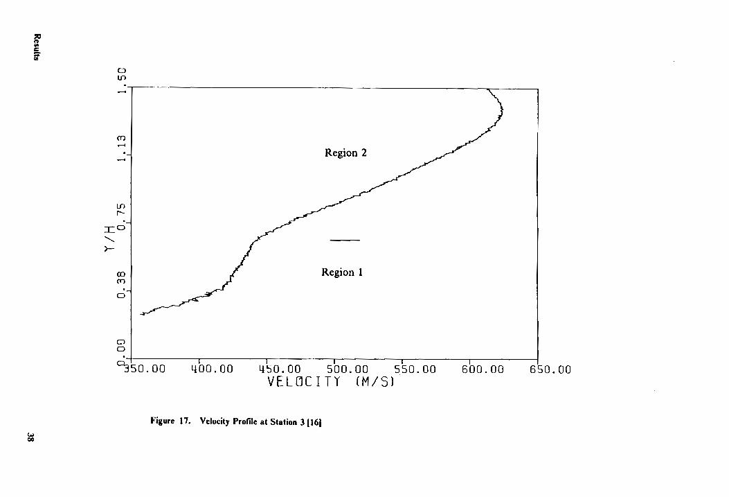
Figure 17. Velocity ProfIle at Station 3 [16] ............................. 38

Figure 18. Average Structure Angles at Station 4 ......................... 39

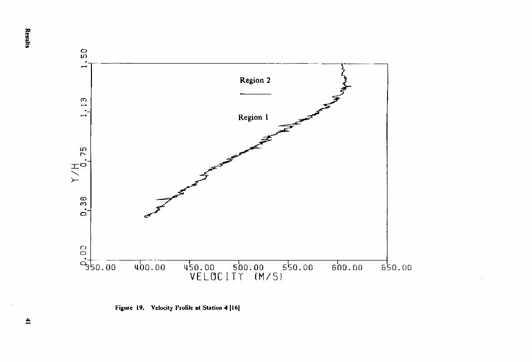
Figure 19. Velocity ProfIle at Station 4 [16] ............................. 41

List of Illustrations vi

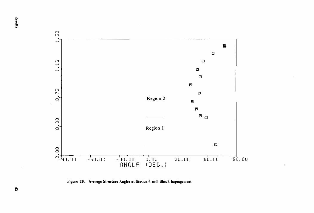
Figure 20. Average Structure Angles at Station 4 with Shock Impingement ...... 42

Figure 21. Velocity Profile at Station 4 with Shock Impingement [16] .......... 44

Figure 22. A verage Structure Angles at Station 4 without Shock Impingement ... 45

Figure 23. Average Structure Angles at Station 4 with and without Shock ...... 46

Figure 24. Average Structure Angle Results at Stations 2, 3, and 4 ............ 49

Figure 25. A verage Structure Angle Results for Three Data Sets at Station 4 .... 50

List of Illustrations vii

Nomenclature

8 w

u l'

S11

S12

HW1

HW1RMS

HW1

HW1RMS

y

t

M Pt

Tt

d H X y

Nomenclature

average structure angle

wire separation distance (1.33 rom)

local mean velocity

time delay between hot wire signals auto-correlation of hot wire signal

cross-correlation of hot wire signals

data from the upper hot wire

root mean square of data from the upper hot wire data from the lower hot wire

root mean square of data from the lower hot wire time shift applied in correlation time

Mach number

total pressure

total temperature

boundary layer thickness slot height

streamwise position referenced from slot injection vertical position referenced from the floor of the test section

viii

1.0 Introduction

Recent interest in developing an air breathing hypersonic vehicle with supersonic

combustion has prompted research in studying the effects of slot injection into a

supersonic flow. If fuel is injected tangent to the flow through a slot, the walls of the

combustion chamber can be cooled in addition to adding fuel [1]. This particular study

utilized supersonic injection, which would provide additional thrust in the propulsion

system [2]. For a hypersonic engine with an inlet Mach number between 8 and 10, the

Mach number in the combustion chamber would approach 3. As a result, a freestream

Mach number of 3 was chosen for this study.

The specific thrust of this research was to study the characteristics of organized

structures throughout the flowfield. In recent years, much research has been dedicated

to the study of turbulent structure. Recent studies indicate the existence of a complex

deterministic hierarchy of structures [3]. The existence of the structures has been

associated with turbulent energy.

Studies of organized structures in turbulent boundary layers flISt began in 1967 when

Kline proposed the bursting cycle [4]. Kline proposed that the bursting phenomenon

stimulates the production of turbulent energy and controls the diffusion of this energy

from the inner to the outer layer. Later work by Corino and Brodkey [5] indicated that

Introduction

the bursts account for approximately 70% of the Reynolds stress level in the boundary

layer near the wall. Kim et. al. [6] later showed that the majority of the net production

of turbulent energy in the range of 0 < y+ < 100 occurs during bursts. As a result,

interest developed in the interaction between the inner and outer layer structures and the

large scale, outer layer structure of the boundary layer. Studies by Brown and Thomas,

Chen and Blackwelder, Moin and Kim, Thomas and Bull, Rajagopalan and Antonia, and

Robinson have also suggested the existence of a hierarchy of organized structures

[7,8,9,10,11,12,].

Head and Bandyopadhyay later used flow visualization to study zero pressure gradient

boundary layers over Reynolds numbers ranging from 500 to 17,500 [13]. They observed

"hairpin" vortices which appeared to exist throughout the boundary layer. A sketch of

the structure is presented in Figure 1. These hairpin loops appeared to be inclined to the

wall at a characteristic "eddy angle'" of 4OO - 500. The structures appeared to describe the

whole of the boundary layer. While most of the research in this area has been dedicated

to the study of incompressible flow, Robinson observed structures in supersonic flow

which were similar to those found in incompressible flows [12]. Recent studies by Spina

and Smits indicate the existence of organized structures in a zero pressure gradient

supersonic turbulent boundary layer [3J. Small angles were measured near the floor;

however, the angles increased to approximately 450 and remained constant throughout

700/0 of the boundary layer. The angle tended toward 9OO near the edge of the boundary

layer. Similar results were obtained in studies of organized structures of a supersonic

boundary layer subjected to short regions of concave surface curvature by Donovan and

Smits [14]. Perturbations of the flowfield tended to increase the inclination of the

structure angle near the wall. In the present study, the existence of organized structures

in a supersonic slot injected flow field was investigated.

Introduction 2

.) lift-up and osc111ation

b) initiation of vort.x roll-up

Vorticity ·Sheet" I

c) vortex dtv.lopment: ~11'1clt10n and concentration

5tr .... 1s. Yortlx Stretc:1ng

/

d) vortex ejection. stretching Ind ... terlction

Figure 1. Hairpin Vortices During the Bursting Process (15)

Introduction 3

The supersonic wind tunnel and the experimental model are described in Chapter 2.

Means of obtaining measurements of the structure angles are presented in Chapter 3.

A zero pressure gradient supersonic boundary layer was studied upstream of the slot

injected flowfield for a consistency check. Results from this study are presented in

Chapter 4. Results obtained from studies of the supersonic slot injected flow field are

discussed in Chapter 4 as well. Conclusions are presented in Chapter 5. All other

aspects of the experiment are included in the Appendices.

Introduction 4

2.0 Experimental Background

Experiments were conducted in the VPI&SU 23 cm x 23 cm "blow-down" supersonic

wind tunnel. The tunnel control valves, the traversing mechanism, and the data

acquisition were all controlled by an IBM PC which contained a MetraByte

analogi digital, digital/ analog, input/ output board. Total pressure and temperature were

monitored in the settling chamber upstream of the nozzle block. Flowfield

measurements were obtained with high frequency response hot-wire anemometers, and

data were recorded via a LeCroy analogI digital data acquisition system. Details of the

wind tunnt.~ and the experimental model are included in the following sections.

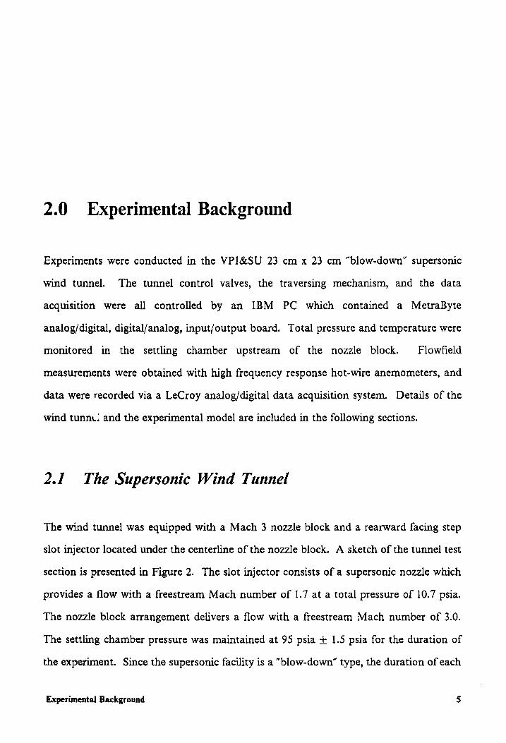
2.1 The Supersonic Wind Tunnel

The wind tunnel was equipped with a Mach 3 nozzle block and a rearward facing step

slot injector located under the centerline of the nozzle block. A sketch of the tunnel test

section is presented in Figure 2. The slot injector consists of a supersonic nozzle which

provides a flow with a freestream Mach number of 1.7 at a total pressure of 10.7 psia.

The nozzle block arrangement delivers a flow with a freestream Mach number of 3.0.

The settling chamber pressure was maintained at 95 psia ± 1.5 psia for the duration of

the experiment. Since the supersonic facility is a "blow-down" type, the duration of each

Experimental Background 5

r .. g' rt a I!.. = ~ lII:'"

(lei .. o c i.

QI.

<t

Figure 2. Sketch or Tunnel Test Section

Nozzle Block

M = 3.0 Siol (12.1 mm)

~ I M = 1.1 -.............. -==ro.o-----------TI-(--:-:-::(:.:c:1;1 Test Se:ion Plate

I \ I

SIOl Injector

run is less than ten seconds. The stagnation temperature also decreases approximately

5° C during the run.

Air is compressed by four Ingersoll Rand, Model 90, reciprocating compressors. The

air undergoes a drying and filtering process and is stored in 16 tanks with a total volume

of 75 cubic meters. In addition to supplying air for the supersonic wind tunnel, air is

bled from the storage tanks for the slot injection system.

The settling chamber contains probes for measuring total pressure and temperature.

Butt .. welded 3.9 micrometer diameter Type K thermocouple wires were used to measure

the temperature. The output signal was amplified and low pass filtered before sampling.

The stagnation pressure is regulated by a fast hydraulically controlled servo valve. The

servo valve is controlled by an analog servo control circuit which in turn receives an

analog voltage from the digital/analog MetraByte board.

2.2 Experimelltal Model

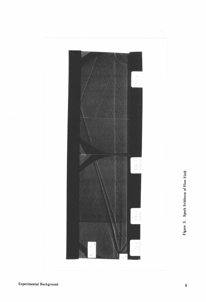
A Spark Schlieren of the flowfield is presented in Figure 3. The flow is from left to right.

As can be seen, the flowfield consists of the slot injection boundary layer near the floor

of the test section, the slot injection freestream, a mixing region, and the tunnel

free stream. The slot height is 1.27 cm. The turbulent boundary layer thickness on the

wall approaching the slot is approximately 1.0 cm. As can be seen from the photograph,

the injected flow is slightly overexpanded. An adjustment shock and its reflection in the

injectant stream can be seen just after the slot. The shear layer deflects toward the wall

initially indicating a slightly overexpanded injection condition. The "lip" shock can be

seen propagating into the freestream [1].

Experimental Background 7

Experimental Background

,..; " . .. :::I .~ \.1.0

8

Four stations are noted at the floor of the model; however, the flowfield was not studied

at station 1. Measurements were obtained at stations 2, 3, and 4 corresponding to X/H

of 4.0, 10.0, and 20.0 respectively. The ratio, X/H, corresponds to the distance from the

slot injector divided by the slot height. Effects of the lip shock as well as the adjustment

shock can be seen at station 2. The tunnel freestream, the mixing region, the slot

injection freestream, and the slot injection boundary layer are all distinct at station 2.

At station 3, the mixing region and slot injection boundary layer begin to merge. The

two flows appear completely mixed after reaching station 4. The lip shock reflection can

be seen at station 4 in the upper part of the tunnel freestream. Detailed measurements

of the flowfield at the previously mentioned stations have been made with pitot and

cone-static probes to determine mean profiles [16]. Hot-wire measurements were

obtained previously to determine the mass flux. The two-dimensionality of the flowfield

was checked [2].

In addition to studying the previously mentioned stations, the flowfield was studied 0.5

inches upstream of the slot injection in the turbulent boundary layer. The upstream

station can be denoted station -1 (not shown in Figure 3). Measurements were obtained

on the upper side of the splitter plate in the region of a supersonic zero pressure gradient

boundary layer. As discussed earlier, previous studies of supersonic zero pressure

gradient boundary layers suggest the existence of organized structures throughout the

boundary layer. Results obtained at station -1 were compared with previously published

data as a consistency check.

2.3 Experimental Control System

Experimental Background 9

Tunnel

<: Q - -.. 0 -<

'0 .. -d 0 U E-- Q c: r-: Go)

d > d -l :So E-

MetraByte

ffiEB VMI

Mainframe

Figure 4. ExperimentaJ Control System

ExperimentaJ Background

HWI DISA Constant

U <: -~ --

Temperature

Anemometers

IFA Signal

Conditioners

U U U Q <: 0

- N M

~ ?: ::: - - -.... .... ......

Lecroy

AID Converter

I

10

The experimental process was controlled with an IBM PC containing a MetraByte AID,

DIA, input/output board described in references [1] and [20]. A schematic of the

experimental control system is presented in Figure 4. The tunnel control valve,

stagnation pressure, and the LeCroy AID data acquisition system were all controlled by

analog outputs from the MetraByte board. The digital inputs were varied within a

FORTRA:'1 program by implementing software supplied by MetraByte. The program

is discussed in greater detail in Appendix A. Commands for controlling the speed,

positioning, and sequence of the traverse were also imbedded in the program.

2.4 Traversing System

The hot-wire probes were mounted in a traversing mechanism located under the floor

of the test section of the wind tunnel. The mounting system consisted of a clamping

mechanism for the probe which was bolted to a rack. The rack was driven by a stepper

motor with a pinion. A LYNN products stepper controller, Model 3701, was used to

control the input to the stepper motor driver. The rotational speed, angular

. displacement, and direction of rotation were controlled. An assembly language program

was compiled and utilized in conjunction with the FORTRAN program controlling the

tunnel operation (17]. The stepper motor can be operated at a maximum rotational

speed of 500 rpm, which corresponds to a vertical speed of 22.1 em/ s.

The vertical position of the hot-wire probe was determined from the output of a

Trans-Tek 245 Linear Voltage Displacement Transducer (L VDT), DC input and output.

The L VDT housing was clamped to the support frame of the traversing mechanism, and

the core was attached to the rack. The useable working range of the L VDT was 10.2

Experimental Background 11

cm. A Bessel filter was designed and built to eliminate the 2 kHz oscillation present in

the LVDT output signal [18]. A cathetometer was used to calibrate the traverse. For

a given location of the probe, the output from the L VDT was recorded. The

corresponding vertical distance of the hot wire from the floor of the tunnel was measured

with the cathetometer. The cathetometer could be read to within 0.001 cm; however,

measurements were accurate to ± 0.010 cm. The accuracy of the measurement was

obtained from a single sample statistical analysis which is included in Appendix B.

Experimental Background 12

3.0 Measurement of Structure Angles

The thrust of the experiments was to determine if organized structures existed in the

flowfield and if so, the corresponding structure angles. A parallel array dual wire probe

and two separate hot-wire anemometers were used to measure flowfield characteristics.

The hot-wires were oriented parallel to the floor of the tunnel. A LeCroy bigh speed

data acquisition system was employed to record data. Implementation of this equipment

as related to determining the structure angle is described in the following sections.

3.1 H{)t- Wire Probe and Anemometers

A DISA model 55P71 parallel array dual hot-wire probe with a flXed separation distance

between hot-wires of 1.33 mm was used. A sketch of the hot-wire probe is presented in

Figure 5. The separation distance, time delay between measurements and local velocity

are all used to obtain the local structure angle. The local velocity is obtained from

velocity profiles resulting from pitot and cone-static probe measurements. Although

calculation of average structure angles depends upon results from the velocity profiles,

hot-wire data used to determine the time delay between measurements are obtained

independently from mean flow measurements. In Figure 6, a triangle is constructed

showing the relation between the previous parameters. F or a given wire separation

Measurement of Structure Angles 13

Flow Direction

r-- 33

100

Side View of Hot Wire Probe

Wire length: 1.25 rom

Wire diameter: 5J.U1l 46.3 r-

r- 8 ~t--- 33 ~, --L

(h = __ ~'--________ --'-_""'= 2.3

T T All dimensions in millimeters

Figure S. Sketch or Hot Wire Probe

Measurement or Structure Angles 14

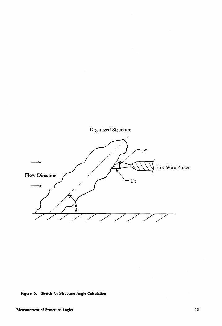
Organized Structure

w

Flow Direction

Figure 6. Sketch for Structure Angle Calculation

Measurement of Structure Angles 15

distance, a structure passing the parallel wire probe at a given angle will cause a time

delay between the output of the hot-wires. If this time delay is multiplied by the local

velocity, a dimension of the triangle can be obtained. From trigonometry, the structure

angle associated with an average large-scale motion can be calculated as follows:

8 -1 W = tan -­UT (1)

The dual wire probe was connected to two DISA 55DOI constant temperature

anemometers. The two hot wires were made of platinum plated tungsten wires of 5

micrometer diameter and 1.25 millimeter length.

A schematic of the constant temperature anemometer is presented in Figure 7. The hot

wire is used as a sensing element of the Wheatstone bridge. Flow past the wire tends to

cool the wire, which in tum reduces the resistance of the wire. The bridge becomes

unbalanced, and this unbalance is sensed and corrected by increasing the input voltage

to the bridge. The resulting increase in current increases the sensor temperature and

resistance. As a result, the input voltage is proportional to the convective heat loss and

can be monitored to determine flowfield characteristics such as mass flux and

temperature [19]. In this experiment, the hot wires were used to determine average

angles of organized structures which exist in the supersonic flowfield.

Frequency response of the anemometers was of prime importance since the flowfield was

supersonic. The bridge of the DISA 55DOI anemometer could be adjusted to yield a

1:20 or a 1:1 ratio. The bridge ratio is simply R2 /Rw. Greater frequency response was

obtained with the 1: 1 bridge ratio and was therefore used in the experiments. An

external resistance circuit was built to vary the overheat ratio of the hot wire. This

circuit allowed the user to adjust the resistance of the bridge. Circuits were designed

Measurement of Structure Angles 16

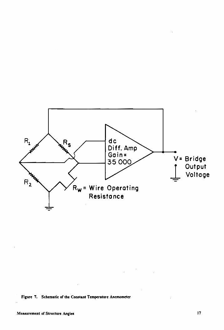
Rw= Wire Operating Resistance

Figure 7. Schematic of the Constant Temperature Anemometer

Measurement of Structure Angles

V= Bridge

1 Output Voltage

17

such that the two hot wires could be operated at the same overheat ratio of 1.8. Means

of adjusting inductance and conductance were built into the anemometer.

Once the bridge was balanced, the anemometer amplifier characteristics could be

adjusted to increase the frequency response of the hot-wire probe and anemometer. A

sine wave test was performed to determine the frequency response of the hot wires [20].

Frequency response curves were obtained in the freestream of the tunnel at Mach 3.0.

The frequency response of the hot wires was approximately 160 kHz [20].

After tuning the hot wires, each hot wire was checked during a run to determine if strain

gaging effects were prevalent. A resonance of the hot wire, typically at 13 kHz, was an

indication of strain gaging. Probes with hot wires exhibiting this characteristic were not

used.

3.2 Allalog/ Digital Data Acquisition

Data acquisition was performed with two LeCroy model 6810 waveform recorders and

the analog/digital portion of the MetraByte board. The LeCroy model 6810 is a 12 bit

vertical resolution, 1, 2, or 4 channel simultaneous waveform recorder. The 6810

contains 512 kBytes of memory and is capable of sampling at 5 MHz. The full scale

input range may be adjusted to suit the experiment. The range can be varied from 400

mV to 100 V, and a DC offset may be added or subtracted from the range as well. The

memory of the waveform recorder may be segmented, allowing the user to control the

number of samples to be stored in memory after each trigger event. Trigger options

include manual, internal, and external.

Measurement of Structure Angles 18

The LeCroy model 6810 was used in conjunction with an IBM PC. An lEEE·488

standard CGPIB) interface, a GPIB cable, and PC based WAVEFORM CA TAL YST

Oscilloscope software allowed the user to integrate the IBM PC into a multi-channel

waveform recording system [21]. A 20 megabyte hard drive was installed in the PC for

recording data. After sampling, the data were recorded to the hard drive and displayed

on the monitor.

The MetraByte board is capable of both D/A and A/D input/output. Data such as total

temperature and pressure were recorded with the MetraByte at a sampling rate of 1 kHz.

The signals from the hot wires were recorded with the LeCroy. The sampling rate was

set at 2 MHz, and 32,768 samples were obtained per channel. The 2 MHz sampling rate

was required to resolve the average angle of the organized structure. A more detailed

discussion of this requirement is presented in Appendix C. An anti-aliasing filter was

employed to prevent high frequency content from folding back into the data. The filter

was set at 900 kHz, which sufficiently filtered the output. Details of the hardware and

software required for the automated data acquisition process are presented in Appendix

A.

The system was tested to determine if any inherent time delay between recording

channels of the LeCroy was present. A 200 kHz square wave was sampled at 2 MHz

on 2 channels. Transition from high to low voltage occured at the same discrete time.

This test was important since calculation of average structure angles is dependent upon

the time delay observed between the two signals.

Measurement of Structure Angles 19

3.3 Data Reduction

The time delay between the data resulting from the two hot-wire signals was obtained

by performing a cross-correlation of the two signals. The cross-correlation function

provides a means of determining the dependence of one signal on the other. The

cross-correlation may be positive or negative; however, its magnitude wiIllie between -1

and 1 if the function is normalized. The function can be normalized by dividing by the

root mean square of the two functions being correlated. The cross-correlation is defined

by:

(2)

A cross-correlation between two hot-wire outputs yields a phase and magnitude of

correlation between the measurements. For example, if the two measuring systems

detect the same signal simultaneously, the peak value of correlation will occur at zero

time shift (y = 0). If the two measuring systems detect a signal at a discrete different

time, the peak value of correlation will result at the corresponding time shift.

This particular feature provided a means of determining the associated angle of an

organized structure. If an average large-scale structure has an angle of inclination

downstream as seen in Figure 6, the upper hot wire will detect the effects of the structure

prior to the lower hot wire. The data set from the lower hot wire was shifted in time to

determine the cross-correlation. A peak correlation occuring at some positive time shift,

y, indicates a structure with an angle inclining downstream. A plot of a typical

cross-correlation with a maximum at a nonzero time delay is presented in Figure 8. The

Measurement of Structure Angles 20

o o -o CX)

· o

o -(0

1L.. " LLO lLJ ID U

Z~ O· _0

I­a: ....J We a::C\.I a:: • DO U

e o · o

e N

· o~ ________ ~ ________ ~ ________ ~ ______ ~~ ______ ~ ________ ~ 1-30.00 -20.00 -10.00 0.00 10.00 20.00 30.00

Figure 8. Typical Cross-Correlation

Measurement or Structure Angles

.:ill. lJ

21

nonzero time delay between the data sets is represented by the symbol T. The time scale

was nondimensionalized based on the freestream velocity and the boundary layer

thickness. A discussion of the nondimensional parameters is presented in Appendix D.

A computer program was written to determine both auto .. correlations and

cross-correlations. Details of the program are presented in Appendix E. The

auto-correlation can be evaluated as follows:

(3)

The normalized value of the auto-correlation will obviously always have a magnitude

of one and occur at a zero time shift. The auto-correlation function can be integrated

over time to provide the integral time scale. If the integral time scale is multiplied by the

local velocity, a characteristic length of the structure of the turbulence in the flow can

be obtained (22).

Measurement of Structure Angles 22

4.0 Results

A region 0.5 inches upstream of the slot injection was studied. This region provided a

zero pressure gradient supersonic boundary layer which could be analyzed to determine

if present results were consistent with results obtained by Smits [3]. The supersonic slot

injected flowfield was then studied at stations 2, 3, and 4 corresponding to X/H of 4.0,

10.0, and 20.0. Results obtained at the station upstream of the slot injection and the

subsequent stations of interest are presented in the following sections.

4.1 Mean Flow Profiles

Plots of the velocity profiles at X/H of 4.0, 10.0, and 20.0 are presented in Figures 15,

17, and 19 respectively. As mentioned previously, mean flow profiles were necessary to

calculate the average-structure angle. The structure angle is relatively insensitive to

small variations in the velocity; therefore, the mean velocity is a sufficient

approximation.

Results 23

4.2 Comparison witl, Pllblished Data

Previous studies of zero pressure gradient supersonic boundary layers indicate the

existence of an organized structure. Results indicate an average structure angle which

is small near the floor, increases to about 450 throughout 700/0 of the boundary layer,

and increases rapidly to 900 at the edge of the boundary layer [3]. Before studying the

injected nowfield, the dual wire probe was placed upstream of the slot injection on the

upper side of the splitter plate. The zero pressure gradient supersonic boundary layer

was studied to determine if present results were consistent with previously published

data.

The dual hot-wire probe with a fixed separation distance of 1.33 mm between hot wires

was traversed through the boundary layer. Fixed point measurements were obtained to

map the nowfield. A trace of the fluctuating signal plotted against nondimensional time

is presented in Figure 9. The upper trace corresponds to the upper hot wire (hot~wire

# 1), and the lower trace corresponds to the lower hot wire (hot-wire #2). Regions of

the trace exhibit similar characteristics indicating the passage of an organized structure

larger than the wire separation distance. For the trace presented, a nondimensional time

delay, 't', between the two signals is apparent. The cross-correlations obtained at five

locations are presented with respect to position in the boundary layer in Figure 10.

Values of the cross-correlation reach a high of 0.68 in the middle of the boundary layer,

decreasing only to 0.42 at the edge of the boundary layer. The nondimensional time

delay (or) between signals decreases from 1.8 in the middle of the boundary layer to zero

at the edge of the boundary layer. The highly correlated output coupled with the

nonzero time delay indicates that both wires are detecting the same organized motion.

Results 24

- ('\J

a • W lJ.J a: a: - )-04

::J:. 3:

l- I-e 0 :I: :I:

Results

Ofl"O (A)

Ofl"O-3:J(jllfJA

0 0

0 0 ("f')

0 0

0 U1 C\J

0 0

0 0 C\J

0 a 0 U1 -0 a

0 0 -o a

o U1

o o

sl~

] -

2S

8

8

8

8

8

0.00

J.!.t a

y {)

- 1.0

.0'

"".00

= 0.61

.00

0.46

.00

== 0.31

.00

Figure 10. Cross-Correlations Throughout the Boundary Layer

Results 26

Since the time shift (y) in the correlation program was applied to the output from the

lower wire, a peak correlation occuring due to a positive time shift indicates a structure

inclining downstream.

Results of the structure angle from measurements taken in the boundary layer at station

-1 are presented in Figure 1 I. The angle is nearly 5()O throughout the majority of the

boundary layer and increases to 900 at the edge. Small angles were not detected near the

floor; however, measurements were not taken close enough to the floor with respect to

the bounda:y layer thickness. The boundary layer studied was relatively small compared

to boundary layers previously studied by Smits [3], making near wall measurements

difficult. The boundary layer studied by Smits was 2.8 cm thick, while the boundary

layer of this study was approximately 1.0 cm thick.

Six measurements were taken in the middle of the boundary layer at the same fIXed point

(X/H of 0.24) to detennine an arithmetic mean and corresponding uncertainty for the

time delay between signals. A plot of the cross-correlation between signals for each

measurement is presented in Figure 12. The arithmetic mean of the correlation was 0.66

and the uncertainty was 0.02. The arithmetic mean of the time delay was 5.833 J.l.S with

an uncertainty of 0.4 J.l.s. A mUltiple sample statistical analysis could not be performed

since the time and expense required to repeat the data set was not feasible. To establish

confidence intervals for probe location and structure angle, a statistical approach for

describing uncertainties in single-sample experiments was taken. The statistical analysis

is presented in Appendix B. Results indicate that the probe location lies within a

confidence interval of ± 0.01 cm. The structure angles obtained lie within a confidence

interval of ± 2.10•

Results 27

~ ~ filii

N QO

::L b

o o .-.

Lf)1 r--

0 l.{) . 0

Lf> (\J

ol

o o

en.oo

(!]

l!1

[!} [!]

l!1

[!}

[!]

T 15.00

1- -. I I

45.00 60.00 75.00 1

30.00 90.00 RNGLE (0 E G . )

Figure 11. Angle of Organized Structure Throughout the Boundary Layer

..:

CI N

0 1-30• 00 -15.00

8 ..:

CJ U:I

ci

CJ IV c:i

10 N ,

-!O.OO -15.00

8

0 • c: • o 0 .~

'" ~ 5 2 u .

0

0 N

ci 1-30. DO -15.00

0.00 IS.00 30.00

0.00 IS.00 30.00

0.00 15.00 30.00

Ut T

CJ CJ

..:

CJ CJ

..;

0 U:I

a

0 N

0

0 N

Q 1_30• 00

0 N

a

0 1'\1

ci '-3D. 00

Figure 12. Reliability Measurements in the Boundary Layer

Results

-lS.DO 0.00 15.00 30.00

-15.00 0.00 15.00 30.00

-15.00 0.00 15.00 30.00

29

After duplicating results from previously documented research, a level of confidence was

established in the measuring technique. The goal of this study was to examine the effects

of slot injection on the flowfield and determine if organized structures existed in the

flowfield. After establishing the consistency of the experimental procedure, the injected

flowfield downstream of the splitter plate was studied.

4.3 Criteria For O,lIganized StructuJ"e

In the boundary layer study at station -1, the peak value of the correlation and the

non-zero value of the time delay implied the existence of an organized structure. The

correlation was relatively high throughout the boundary layer indicating the existence

of an organized structure. For the slot injected flowfield, regions of the flowfield are

substantially different. Regions of low correlation or no correlation were expected. A

means of determining if an organized structure existed was necessary.

Each data set was screened to determine if an organized structure passed the hot wires.

Two means of screening the data were used. Initially, the fluctuating time dependent

signals were analyzed. The peak to peak fluctuations of each hot wire were compared

to determine if the hot wires were in the same regime of the flowfield. For example, the

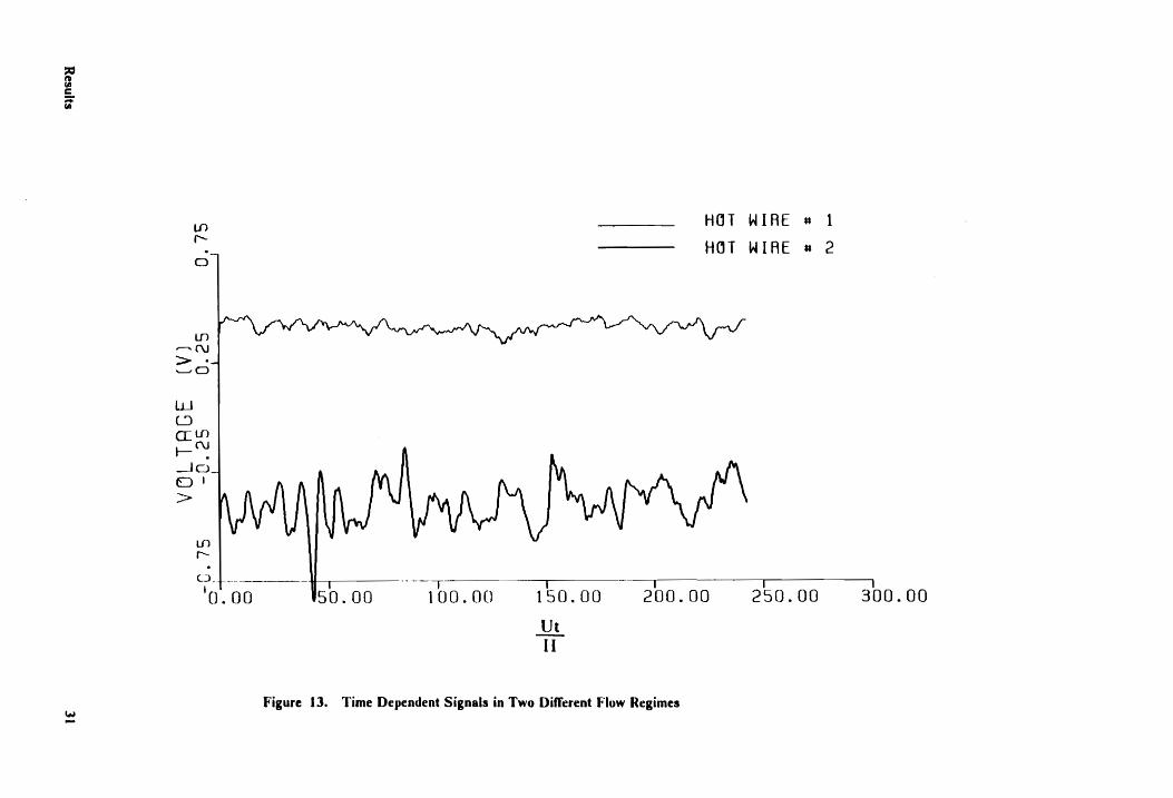
time dependent trace of Figure 13 illustrates the difference in peak to peak fluctuations

for a given fIXed point measurement.

The lower hot wire, corresponding to the lower trace, was in the mixing region of the

flowfield at X/H of 3 and Y /H of 1.5. The upper wire was located above this region in

the tunnel freestream. The traces were further compared to determine if any common

fluctuations were present. The two traces of Figure 13 show no similar character. The

Results 30

!' c :::; III

(N

U1 f-

a

If) ,......., ('\J

> .......... 0

w C)

cr U1 I-{'\J

---10 £) I

>

Ul r-

((o~-oo- 1sb. 00 O. 00 I 150.00

lJt II

Hell WIRE ** 1 Hell WIRE ** 2

I .---. 200.00 250.00 300.00

Figure 13. Time Dependent Signals in Two Different Flow Regimes

final means of screening data was based on results from the cross-correlation. The

cross-correlation of the two time dependent signals of Figure 13 was on the order of 0.1.

In general, cross-correlations with peak values of 0.3 and less were rejected. The peak

value of the cross-correlation was difficult to determine for data sets exhibiting poor

correlation.

4.4 The Supersonic Slot Injected Flowfield

With a means of determining if an organized structure existed, the flowfield was studied

in detail at X/H of 4.0, 10.0, and 20.0. Fixed point measurements were taken at each

station from the floor of the test section to Y/H of 1.5. The ratio, Y/H, corresponds to

the vertical distance from the floor of the test section divided by the slot height. After

studying the flowfield at each station, a compression ramp was used to generate a weak

shock between X/H of 10 and X/H of 20. Measurements were repeated at station 4

(X/H of 20) to determine the effects of the streamwise pressure gradient on the organized

structures. Results from each station are discussed in detail in the following subsections.

4.4.1 Results at Station 2

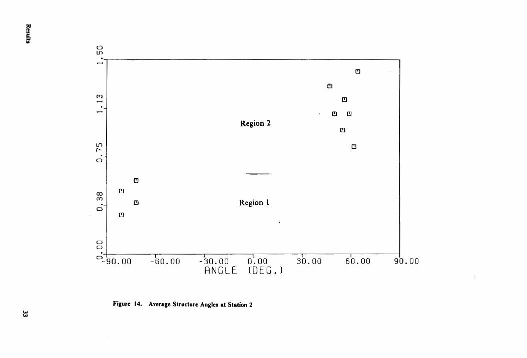
A plot of the average angles of the organized structures at X/H of 4.0 is presented in

Figure 14. As can be seen in the figure, an abrupt transition occurs in the calculated

average structure angles. The plot indicates the existence of distinct regions where the

angles are consistent. In region 1, average structure angles are seen to vary from -720

to -81°, This region is between Y/H of 0.2 and Y/H of 0.6. The second region consists

of average angles on the order of 500 and lies between Y/H 0[0.6 and Y/H of 1.5.

Results 32

if 5. ... •

w w

0 U1

en/ ........

"....... I

Lf)i ,...... .

°1

:~

o o

(!)

[!J

-90.00

[!J

£!l

-60.00 -30.00 RNGLE

Region 2

Region 1

0.00 (0 E G • )

Figure 14. Average Structure Angles at Station 2

I!J

[!)

[!) [!)

[!)

(!)

30.00 60.00 90.00

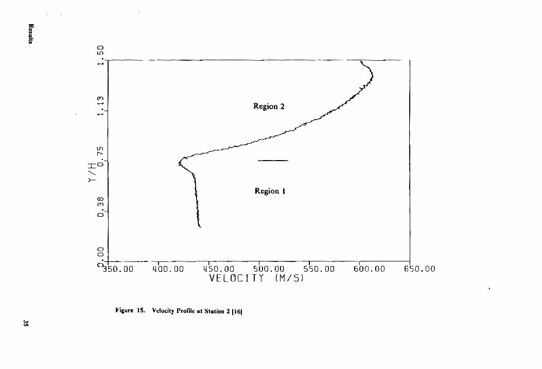
These results may seem confusing at frrst; however, a plot of the velocity profile helps

clarify the results. In Figure 15, the velocity profile [16] is presented with each region

of interest identified. As can be seen from the profile, two different regions can be

identified in the flowfield. The region from Y/H of 0.2 to Y/H of 0.75 consists of the

boundary layer which developed on the underside of the splitter plate used in the

supersonic slot injection. The region from YjH of 0.75 to Y/H of 1.5 consists of the

boundary layer which developed on the upper side of the splitter plate.

As discussed earlier, average angles of organized structures followed similar trends to

boundary layer profiles in zero pressure gradient supersonic flows. The supersonic slot

injected flowfield consists of multiple flowfield profiles at station 2. Two regions were

discussed and labeled in Figure 14. Comparing regions of interest from the velocity

profiles to the distribution of average structure angles, a pattern is recognized. In the

frrst region, the boundary layer resulting from the underside of the splitter plate

corresponds to the region where negative structure angles were obtained. Positive

structure angles similar in magnitude to those obtained upstream at station -1 were

obtained in region 2 where the boundary layer developed off the top of the splitter plate.

4.4.2 Results at Station 3

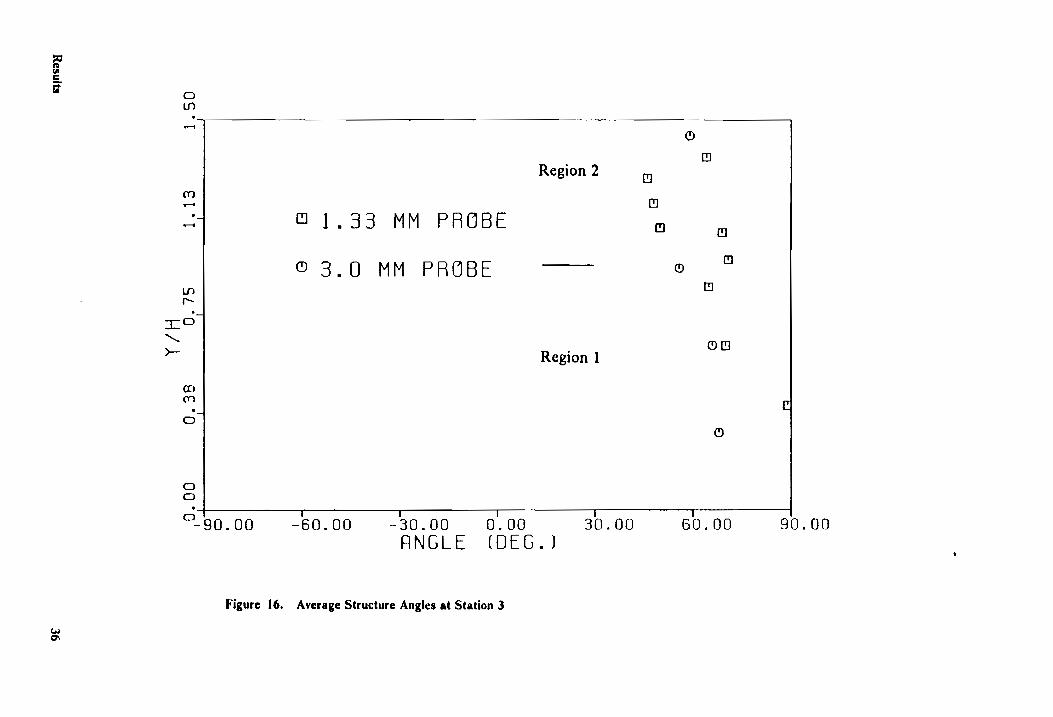
The flow field at station 3 was studied in a similar fashion. A plot of the average

structure angles is presented in Figure 16. Preliminary measurements were made at this

station with a dual hot-wire probe having a wire separation distance of 3 mm. The

corresponding sampling rate was 1 MHz. These measurements were initially obtained

to determine the feasibility of the study. Results of these measurements are included in

Figure 16 and are seen to support the results obtained with the dual hot-wire probe

Results 34

~ c: :; (jII

~

o Ln

........

en -........

Ln ,......

:cO ""­>-

(0

en

o

o o

Region 2

Region 1

~~O. 00 4dO.00 450. 00 SOD. 00 550.00 600. 00 6~0. 00 VELOCITY (MIS)

Figure I S. V clocity Profile at Station 2 116)

::0 ftI (I)

s:: if

~

° If)

........

~I -I

If) I

f"'-a

ID '-.. >-

(D en . 0

o o

-90.00

[!] 1.33

(!) 3. 0

-60.00

Region 2

MM PROBE

MM PROBE

-30.00 ANGLE

Region 1

0.00 (OEG.)

30.00

Figure 16. Average Structure Angles at Station 3

(9

(!]

[!]

[!]

[!] [!]

(!) [!]

(!]

(9f]

(!)

60.00 90.00

having a wire separation distance of 1.33 nun. Measurements were also made at station

2 with the hot-wire probe having a wire separation distance of 3 nun; however the

organized structures could not be resolved due to poor correlation between signals.

An average structure angle of 68° was obtained in region 1 which ranged from Y/H of

0.35 to Y/H of 1.0. From Y/H of 1.0 to Y/H of 1.5, a region consisting of average

structure angles of 500 appeared. Refering to the velocity profile [16] for station 3 in

Figure 17, trends become more apparent. After reaching X/H of 10.0, the boundary

layer from the upper side of the splitter plate began to merge with the slot injected

flowfield. Distinct regions due to slot injection are not as prevalent; however, varying

regions in the profile do exist. In region 1, the profile appears consistent with the

structure angles obtained. Angles on the order of 650 were obtained in this region.

Structure angles measured in region 2 also followed trends of the velocity profile in this

region. A verage structure angles on the order of 500 were obtained in this region.

Similar measurements were obtained at station 2 in the same region. This region

appears to be the remnant of the structure angles measured upstream at station -1.

4.4.3 Results at Station 4

Station 4t l:orresponding to 20 slot heights from the slot injection point, was the last

station studied. The flowfield was well mixed at this station since the boundary layer

from the splitter plate and the floor of the test section were completely merged. A plot

of the average structure angles is presented in Figure 18. Results obtained using the dual

hot-wire probe with a wire separation distance of 3 nun are again superimposed on this

plot. These results support the trends obtained with the dual hot-wire probe having a

wire separation distance of 1.33 mm.

Results 37

~ c if

~

o 1.11

..-.

m .--f

......

1.11 r-.

IO "­>-

co en

o

G)

o • I ~50. 00 400.00

Region 2

Region 1

450.00 500.00 550.00 VEL(j[ I TY (MIS)

Figure 17. Velocity Profile at Station 3 (l6J

600.00 650.00

~

'"

o o

-60.00 -30.00 ANGLE

0.00 (0 E G • )

Figure 18. Average Structure Angles at Station 4

30.00 60.00 90.00

Measurements indicate an average structure angle of approximately 600 from Y/H orO.2

to Y/H of 0.7. Measurements obtained in region 2, corresponding to Y/H of 0.7 to Y/H

of 1.5, indicate average structure angles on the order of 500• The region from Y/H of

0.2 to Y/H of 0.7 is similar to that obtained at station 3 with average structure angles

of 600. Region 2 appears consistent with measurements obtained at Y/H of 0.7 to Y/H

of 1.5 at the previous two stations. Average structure angles of 500 were obtained in this

region. These regions are dominated by the merged boundary layers which can be seen

from the velocity profile [16J of Figure 19. Structure angles obtained in the upper part

of region 2 appear to be increasing. The freestream of the tunnel can be seen in the

upper part of region 2. The structure angle was expected to approach 900 in this region

as was noticed in the study of the zero pressure gradient supersonic boundary layer

studied at station -1.

4.4.4 Results at Station 4 with Shock Impingement

A compression ramp was bolted to the test section of the tunnel to generate a weak

shock wave. The shock wave fell between station 3 and station 4. Measurements were

repeated at station 4 to determine the effects of the streamwise pressure gradient on the

organized structures. This data set was obtained approximately two months after the

data set previously discussed.

Results from these measurements are presented in Figure 20. Two regions of interest

are apparent in this figure. In region It ranging from Y/H of 0.2 to Y/H of 0.4, structure

angles on the order of 620 were obtained. From Y/H of 0.4 to Y/H of 1.2, structure

angles on the order of 500 were obtained. This region corresponds to the boundary layer

Results 40

::0 II foil C ::;' foil

.Ill> -

0 U1

........

en ........

....:-1

If)

r-. IO "'­>-

ro m

o

o o

400.00

Region 2

Region 1

450.00 500.00 550.00 VELCjC I TY (MIS)

Figure 19. Velocity Profile at Station 4 (16)

600.00 650.00

~ m E. -(jt

.a:.. N

0 If)

......

~I

~~ co· en 01

o o

CJ

Region 2 (!]

Region 1

m [!)

[!]

(!]

[!]

(!]

(!]

(!] CJ

(!]

o I I I I I I I 90.00 -60.00 -30.00 0.00 30.00 60.00 90.00

RNGLE (OEG.)

t'igure 20. Average Structure Angles at Station 4 with Shock Impingement

which developed on the upper side of the splitter plate. The upper part of region 2

approaches the tunnel freestream, and structure angles tend toward 900 .

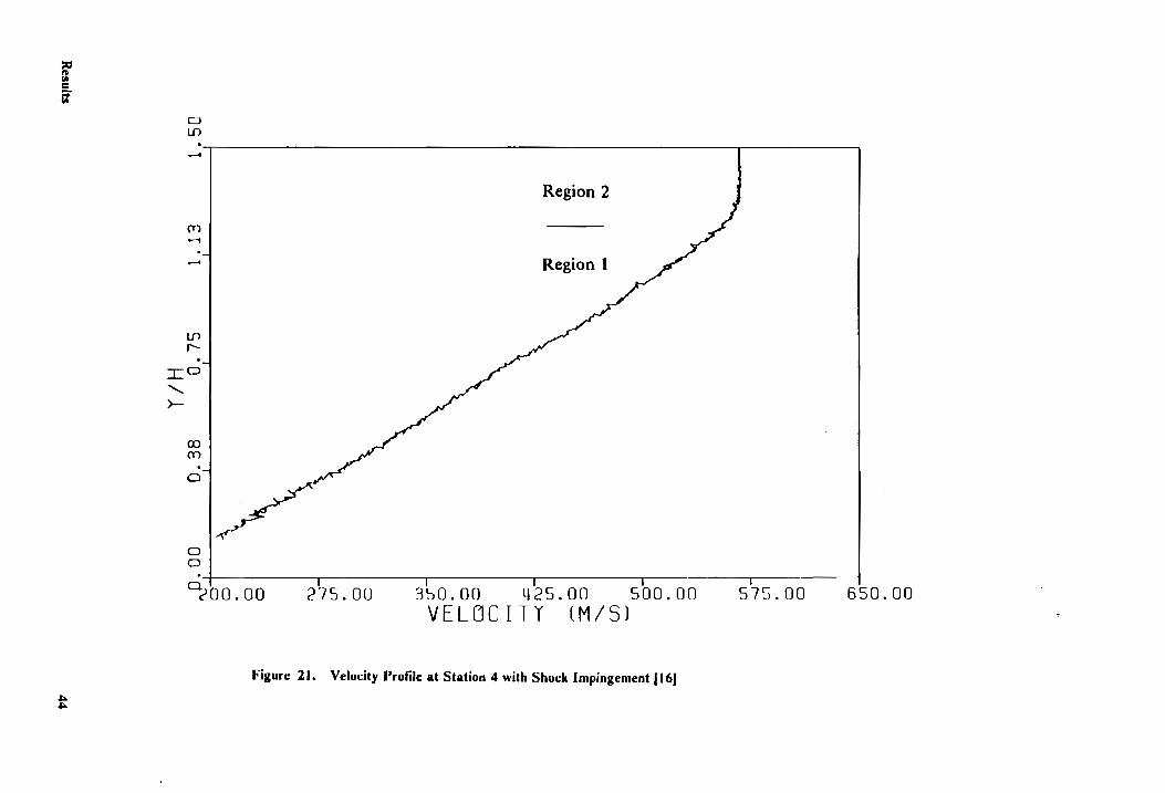
These results were compared with the velocity proflle [16] obtained for the flowfield with

shock impingement at station 4 in Figure 21. The streamwise pressure gradient resulting

from the shock impingement served to reduce the velocity throughout the profile. A

comparison of Figure 19 and Figure 21 readily supports this conclusion. Two regions

were labeled on the velocity profile of Figure 21. Structure angles varying from 65° to

500 were seen to dominate region 1 of the velocity profue. The second region of the

velocity profIle approaches the freestream, and structure angles are seen to tend toward

900 in this region.

Since measurements for studying the effect of the shock impingement were taken at a

later date, the compression ramp was removed from the test section and the unperturbed

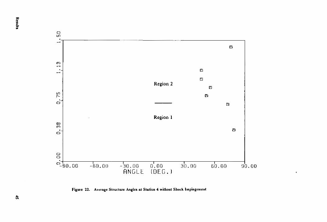
flowfield was again studied at station 4. Results from these measurements are presented

in Figure 22. Three regions can be identified. Region 1, varying from Y/1-I of 0.3 to Y/H

of 0.75 consists of structure angles on the order of 700• In region 2, structure angles

on the order of 500 were obtained. This region ranges from Y/H of 0.75 to Y/H of 1.1

and appears to be the remnant of the boundary layer which developed on the upper side

of the splitter plate. Finally, the third region suggests an increase in structure angle.

The increase toward 900 is to be expected approaching the tunnel freestream.

A comparison was made between measurements taken at station 4 with and without

shock impingement. Results from this comparison are presented in Figure 23. Angles

of the organized structures appear relatively unaffected by the streamwise pressure

gradient created by the shock between station 3 and station 4. Some deviation was

observed in the lower region, ranging from Y/H of 0.2 to Y/H of 0.6; however, this

Results 43

:::0 Jl c if

.c.. .c..

D Ln

........

en ........

'-:1

Ln ,.......

ID ...........

>-

CD en

o

o o

Region 2

Region I

00.00 275.00 350.00 425.00 500.00 VELDC I T Y (MIS)

Figure 21. Velocity Profile at Station 4 with Shock Impingement (16)

575.00 650.00

::;Q 1: e. -fjI

t:i

o If)

.........

en .........

"':1

~I . 01

COl (Y) .J

0

o a

-60.00 -30.00 ANGLE

Region 2

Region 1

0.00 (0 E G • )

[!]

[!]

[!)

30.00

Figure 22. Average Structure Angles at Station 4 without Shock Impingement

[!]

[!]

(!)

[!)

60.00 90.00

:;0 fl c iZ

~

0 to

..-.

~

(!)

:~ (!)

CJ WITHOUT SHOCK ~(!)

[!] ~

(!) WITH SHDCK (!) ~

I~~ m (!) [!J

..........

>-

(0' en .J 0

o o

(!)

(!) (!)

(!]

(!)

~I I I j I I I -90.00 -60.00 -30.00 0.00 30.00 60.00 90.00

ANGLE (DEG.)

Figure 23. Average Structure Angles at Station 4 with and without Shock

deviation could be due to fluctuations in the slot injected stream since the slot injected

stream was not controlled as accurately an the tunnel flowfield.

4.5 Integral Time Scale Results

An auto-correlation was performed on each data set to determine the integral time scale

and corresponding characteristic length. Nearly 50% of the results indicated an integral

time scale of 6 microseconds or less. The frequency response of the hot wires was

approximately 160 kHz; therefore, time scales of 6 microseconds and less could not be

resolved. A time scale of 6 microseconds and less corresponds to a length scale of 3.5

mm and less. Length scales of this order dominated the boundary layer upstream of the

slot injection and the mixing region of the flowfield at stations 2, 3, and 4.

Measurements obtained within the frequency response of the hot wires indicated

characteristic lengths of turbulent structures ranging from 3.5 mm to 21 mm near the

freestream of the tunnel and slot injection.

4.6 Summary

A zero pressure gradient supersonic boundary layer was studied upstream of the slot

injection for a consistency check with previously published data. Structure angles

obtained varied from SOO throughout the majority of the boundary layer to 900 at the

edge of the boundary layer. Structure angle calculations are dependent upon results

from the velocity profiles; however, hot-wire data for correlation purposes were obtained

independently of mean flow measurements. Although measurements were obtained by

Results 47

two different means, structure angle measurements obtained from hot-wire data served

to describe trends of the velocity proftles obtained with pitot and cone~static probes at

stations 2, 3, and 4.

Propagation of structure angles downstream appeared consistent in regions exhibiting

similar flowfield profIles. In Figure 24. results from stations 2, 3, and 4 are presented.

Regions I and 2 appear consistent from one station to the next. Angles on the order

of 650 are prevalent in region 1, which consists of the shear layer between the supersonic

slot injection stream and the supersonic flowfield. Structure angles obtained in region

2 appear to be the remnants of the structures observed upstream in the supersonic

boundary layer at station -1. A verage structure angles on the order of 500 were obtained

in this region. Near the freestream structure angles approach 900.

Results of structure angle measurements at station 4 with and without shock

impingement were compared. The streamwise pressure gradient appeared to have

negligable effect on the organized structures. A further comparison of data sets obtained

at station 4 gives an indication of repeatability. Results from three different data sets

are presented in Figure 25. The legend provides information concerning the results. The

wire separation distance is included as well as a number to indicate if measurements were

obtained the same day. Only one data set was studied with shock impingement, and this

is noted on the legend as well.

From Y/H of 0.75 to Y/H of 1.5, structure angles obtained are within a 50 bandwidth.

Greater deviation was noted in the region ranging from YjH of 0.2 to YjH of 0.75:

however, this region is controlled by the slot injection stream. The slot injection stream

was not as accurately controlled as the tunnel freestream, which could explain the

greater deviation in structure angles obtained in this region.

Results 48

f c = ~

~

II

~I

II

".1 • • : • • • II

~d •

•

,DO ~-lo.oo 410 •• 0 -So. 00 0'.00 SL.o. 1b.0D ANGLE (OE6.1

Figure 24. Average Structure Angle Results at Stations 2, 3, and 4

a •

• !! •

tI

• • " :;x::Q GI ..... ... •

I • 0- •

1.00 8 alo.oo .... 0.00 -~o .• O 0'.00 ------sb.oo eb.08 10.00

RNGLE IDEG.I

::0 ft {II

s:: ~

CJ Ln

...-. [!] ~

[!} +

:~ (g-

(J 1. 33 MM (N 0 SHOCK, 1 ) C)

~

(!]A + C) 3. 0 MM (N (J SHOCK, 2) +[!] A

J::~ [!]+ ~ 1.33 MM (N (j SHOCK, 3)

+ (!] A

"'->- + (!]

+ 1.33 MM (SH(jCK p 3) + + (!]

:~ [!] A

(!) (!)

+ 0 0

~-90. 00 I I I I I 60.00 -30.00 0.00 30.00 60.00 90.00

ANGLE (OEG.l

Figure 25. Average Structure Angle Results for Three Data Sets at Station 4 (.A CI

Integral time scales and characteristic lengths obtained by integrating the

auto-correlation function indicated turbulent structures ranging in size from 3.5 mm to

21 mm. Turbulent structures smaller than 3.5 mm appeared to dominate the mixing

region of the supersonic slot injected flowfield and the zero pressure gradient supersonic

boundary layer upstream of the slot injection. The smaller stuctures could not be

resolved due to the frequency response limitations of the hot-wire anemometer systems

used.

Results 51

5.0 Conclusions

Behavior of the average large-scale structure in a supersonic flow with supersonic slot

injection was explored in this study. To determine if the experimental procedure for

obtaining the average structure angle of the organized motions was consistent with

previous studies, a zero pressure gradient supersonic boundary layer was studied.

Results from this study were consistent with previously published data in that a structure

angle on the order of SOO was seen to dominate the majority of the boundary layer. After

determining consistency of the experimental technique, the supersonic flow with

supersonic slot injection was studied. Three stations were considered to determine the

effects of the organized motions on mixing. Stations 2, 3, and 4, corresponding to X/H

of 4.0, 10.0, and 20.0 were chosen. A compression plate was inserted between station 3

and station 4 to generate a weak shock. A· streamwise pressure gradient resulted at

station 4, and measurements were taken to determine its effect on the organized

structures.

The flowfield was studied at each station from Y/H of 0 to Y/H of 1.5. Measurements

obtained in this region mapped the flowfield from the floor of the test section to the

freestream of the supersonic flow. Average structure angles obtained at each station

resulted in distinct regions describing the nowfield. Of particular interest was an

approximate region ranging from Y/H of 0.8 to Y/H of 1.4. Measurements obtained in

Conclusions 52

this region at each station resulted in structure angles on the order of 50°. Structures in

this region appeared to be the remnants of structures observed in the boundary layer

which developed on the upper side of the splitter plate prior to the superonsic slot

injection. Similar trends for structure angles were noted at consecutive stations with

regions exhibiting similar nowfield profiles.

At stations 3 and 4, the boundary layer from the upper side of the splitter plate was seen

to merge with the boundary layer from the supersonic slot injection. At these stations,

a region from Y /H of 0.2 to Y /H of 0.8 was characterized by structure angles on the

order of 650• A verage structure angles tended toward 900 near the freestream of the

flowfield at stations 2, 3, and 4. The organized structures appeared to describe the whole

of the profile at each station of the supersonic slot injected flowfield.

After studying the unperturbed flowfield at stations 2, 3, and 4, a compression plate was

bolted to the test section of the tunnel. A weak. shock resulted between station 3 and

station 4. Measurements were repeated at station 4 to determine the effects of the

streamwise pressure gradient on the organized structures. Structure angles appeared

relatively unaffected by the streamwise pressure gradient. These results were further

compared with previously obtained data to estimate repeatability of the measurements.

Three data sets were compared, each of which were obtained at a different date.

Structure angles obtained from the data sets deviated within a 5° bandwidth.

Repeatability of the measurements was on the order of the 4.20 bandwidth predicted by

the single sample statistical analysis.

Characteristic lengths of the turbulent structures at each station were studied to

determine any trends in the flowfield. Characteristic lengths ranging from 3.5 nun to 21

mm were calculated; however, 500/0 of the data indicated structures less than 3.5 mm.

Conclusions S3

Length scales of this order dominated the turbulent boundary layer upstream of the slot

injection and the mixing region at stations 2, 3, and 4. Data resulting in integral time

scales of 6 microseconds and less, corresponding to length scales of 3.5 mm and less,

could not be resolved since these time scales were not within the 160 kHz frequency

response of the hot-wire anememometer systems. Future efforts should be devoted to

increasing the frequency response of the hot-wire anememeter systems in an effort to

resolve the size of the smaller structures in the mixing region and the upstream boundary

layer.

Conclusions S4

References

1. Walker, D. A., Campbell, R. L. and Schetz, J. A., "Turbulence Measurements for Slot Injection in Supersonic Flow," AIAA Paper 88-0723, Jan. 1988.

2. Rettew, L. A., "The Use of Hot-Wire Anemometry in Studying Supersonic Slot Injection into a Supersonic Flow," Master's of Science Thesis, Virginia Polytechnic Institute and State University, Feb. 1988.

3. Smits, A. J. and Spina, E. F., "The Effect of Compressibility on, the Large-Scale Structure of a Turbulent Boundary Layer," AIAA Paper 87-0195. January 1987.

4. Kline, S. J., Reynolds, W. C., Schraub, F. A. and Runstadler, P. W., "The Structure of Turbulent Boundary Layer," Journal of Fluid Mechanics. Vol. 30, 1967, p. 741.

5. Corino, E. R. and Brodkey, R. S., "A Visual Investigation of the Wall Region in Turbulent Flow," Journal of Fluid Mechanics, Vol. 37, 1969, p. 1.

6. Kim, H. T. Kline, S. J. and Reynolds, W. C., "The Production of Turbulence Near a Smooth Wall in a Turbulent Boundary Layer," Journal of Fluid Mechanics. Vol. 50, 1971, p. 133.

7. Brown, G. L. and Thomas, A. S. W., "Large Structure in a Turbulent Boundary Layer," Physics of Fluids, Vol. 20, No. 10, 1977, p. 243.

8. Chen, C. P. and Blackwelder, R. F., "Large-Scale Motion in a Turbulent Boundary Layer: A Study Using Temperature Contamination," Journal of Fluid Mechanics. Vol. 89, 1978, p. 1.

9. Moin, P. and Kim, J., "The Structure of the Vorticity Field in Turbulent Channel Flow. Part I·Analysis of Instantaneous Fields and Statistical Correlations," Journal of Fluid Mechanics, Vol. 155, 1985, p. 441.

10. Thomas, A. S. W. and Bull, M. K., "On the Roll of Wall-Pressure Fluctuations in Deterministic Motions in the Turbulent Boundary Layer," Journal of Fluid Mechanics, Vol. 128, 1983, p. 283.

References 55

11. Rajagopalan, S. and Antonia, R. A., "Some Properties of the Large Scale Structure in a Fully Developed Turbulent Duct Flow," Physics of Fluids. Vol. 22, No.4, 1979, p. 614.

12. Robinson, S. K., "Space-Time Correlation Measurements in a Compressible Turbulent Boundary Layer," AIAA Paper 86-1130, 1986.

13. Head, M. R. and Bandyopadhyay, P., "New Aspects of Turbulent Boundary Layer Structure," Journal of Fluid Mechanics, Vol. 107, 1981, p. 297.

14. Donovan, J. F. and Smits, A. J., "A Preliminary Investigation of Large-Scale Organized Motions in a Supersonic Turbulent Boundary Layer," AIAA Paper 87-1285. June 1987.

15. Smith, C. R.,"A Synthesized Model of the Near-Wall Behavior in Turbulent Boundary Layers," Proceedings of Eighth Symposium on Turbulence. Department of Chemical Engineering, University of Missouri-Rolla, 1984.

16. Hyde, Randy and Smith, Ben, personal communication.

17. Caldwell, Frank, personal communication.

18. Campbell, R. L., "Experimental Study of Supersonic Slot Injection into a Supersonic Stream," Master's of Science Thesis, Virginia Polytechnic Institute and State University, Nov. 1988.

19. Dally, J. W., Riley, W. F. and McConnel, K. G., Instrumentation for Engineering Measurements, John Wiley and Sons, 1984, p. 470.

20. Walker, D. A. and Ng, W. F., "Experimental Comparison of Two Hot Wire Techniques for Resolution of Turbulent Mass Flux and Local Stagnation Temperature in Supersonic Flow," AIAA Paper 88-0422, 1988.

21. Lecroy Model 6810 Waverform Recorder Operators Manual, Lecroy, Chestnut Ridge, NY, Sept. 1987.

22. Schlichting, Hermann,Boundary-Layer Theory, McGraw-Hill Book Company, 1987, p. 568.

23. Kline, S. J. and McClintock, F. A., "Describing Uncertainties in Single-Sample Experiments,", Mechanical Engineering. Jan. 1953, p. 3.

References 56

Appendix A. Details of Automated Data Acquisition

Process

The Spark Schlieren of the flowfield presented in Figure 3 illustrates the complexity of

the supersonic flow due to the supersonic slot injection. To describe the flowfield

adequately, fixed point measurements were made at X/H of 4.0, 10.0, and 20.0. The

traverse was used to increment the hot wire in intervals of the wire separation distance

(1.33 rom) from the floor of the test section to the freestream. Since the wind tunnel has

a limited run time and requires time for the compressors to replenish the storage tanks

between runs, a means of optimizing efficiency was desired.

The goal was to obtain as many fixed point measurements as possible for each given run.

A method of consistantly triggering the two LeCroy model 6810 waveform recorders was

desired. Since the FORTRAN program was written to control the traversing system as

well as utilize the MetraByte D/A board, a convenient method was available. As

mentioned previously, the traverse could be incremented at constant speeds and

displacements. As a result, the probe could be traversed to a desired position. After

allowing time for the traverse, the MetraByte board could be used to send an analog

signal to the two model 6810 Lecroy waveform recorders. A schematic of the system is

presented in Figure 4.

Appendix A. Details of Automated Data Acquisition Process 57

The external triggering capability of the two units made synchronization possible. An

analog voltage sent from the M etraByte board was applied across the input of the

external trigger of each waveform recorder. Both cables leading to each unit were of the

same length to assure simultaneous triggering. To test the synchronization, a 200 kHz

sine wave was sampled at 5 MHz. No phase shift between the two units was detected.

In the experiment, 4 channels were used, two channels per 6810 unit. Unit A was used

to record each of the two fluctuating hot-wire signal outputs. Unit B was used to record

output from the L VDT and the DC hot wire output. Since mUltiple triggering was

desired at each fIXed point, the memory of each 6810 was segmented. Only five

measurements per run were possible; therefore, five segments capable of recording

32,768 samples per channel were created. A 2 MHz sampling rate was required to

resolve the local structure angle at each point. This requirement is dependent upon the

wire separation distance as well as the local velocity_ An anti-aliasing filter was

employed to prevent high frequency content from folding back into the data. The filter

was set at 900 kHz, which sufficiently filtered the output.

After determining the details of the hardware necessary for tunnel instrumentation, the

software was written. The FORTRAN program used in the automated data acquisition

process follows.

PROGRAM CONTROL C C THIS PROGRAM TAKES DATA EITHER WHILE PROBE IS TRAVERSED OR FIXED C LINK WITH LIBRARIES: DAS16FOR, NUMER C

INTEGER*2 IHOURO,IHOUR1.IMINO,IMINt,.SECO.ISECl,IHUNDO. S DACN,RTNFLG,DATOUT.DATARRAY(28000).BASEADDR. $ STARTC.MODE,ENDCH.NOS,IPAR,DMALEV,CNTl.CNTI. $ INTLEV.IHUNDl,DATO(9).DACNO REAL MAXPSI,SECS,VOLT,TIMEO.TIMEl,TlMDIF character*6 fnaxne(5)

character*42 pgm(2),pgmJ ,pgm2.pgm3,pgm4 character*2 exe l,exe2 ,exe3,exe4,exe5 ,exe6,exe7 ,exe8,exe9 ,exe 1 0 CHARACTER*2 DUMMY

C COMMANDS FOR TRAVERSING SUBROUTINE C YI: EXECUTE PROGRAM ONCE, Y2: EXECUTE PROGRAM TWICE, ETC. c data pgml I 'V400 D200 Zl Rl • / c:: data pgm2 I 'V400 D200 ZJ.) Rl ' I

Appendix A. Details of Automated Data Acquisition Process 58

data pgm3 / 'VIOO 0200 Zl RI Z1J RI . I data pgm4 I'VIO D200 Zl Rl ZJ.) Rl ' I data exe 1 I 'Y l' I data exe2 I 'Y2' I data exe3 I 'Y3' I data exe4 I 'Y4' I data exeS I 'Y5' I data exe6 I 'Y6' I data exe7 I 'Y7' I data exeS I 'Y8' I data exe9 I 'Y9' I data exe 1 0 I 'xx' I

C DIGITAL REPRESENTATION OF TUNNEL PRESSURE DATA DATa /4095,3391,2882,2403,2006.1553,988,475,0/

C

C C

call cinit

write(*,*)'INSURE STEPPER POWER IS ON AND STEPPER RESET' C TRAVERSE IS INCREMENTED UPWARD IN STEPS OR IN ONE FULL TRAVERSE

write(* .*)' input traverse up command' C AS AN EXAMPLE, VIOO D20 ZO Rl C VIOO-SENDS 100 PULSES/SEC TO STEPPER C D20-COMMANDS THE STEPPER TO TURN 20 COUNTS TOTAL C Z1J-COMMAND FOR CLOCKWISE ROTATION, Zl-COUNTER CLOCKWISE C RI-COMMANDS PROGRAM TO REPEAT 1 TIME

read(* ;(A)')pgm( 1) write(* ,*)' input traverse down command'

C SIMILAR TO UP COMMAND, OPPOSITE DIRECfION. I.E. Zl read(* ,'(A)')pgm(2)

C C IF TAKING FIXED POINT MEASUREMENTS, YOU MUST TRAVERSE TO LAST POSTION C TO PREVENT REPEATING MEASUREMENTS.

WRITE(*,*), DO YOU NEED TO TRAVERSE TO LAST POSITION?' WRITE(*,*,. IF YES ENTER 1. IF NO ENTER 0' READ(* ,*)N FLAG IF(NFLAG.EQ.l )THEN

C EXAMPLE' :F LAST POSITION WAS 4 TRAVERSE INCREMENTS UP, INPUT YS WRJTE(*.~)' ENTER TRAVERSE COMMAND (EXAMPLE Y2)'

C

READ(* ;fAY)DUMMY ENDIF

WRITE(* ,*)'INPUT PRESSURE' READ(* ,*)MAXPSI

C PREPARE STEPPER MOTOR TO RECEIVE COMMANDS FOR FIRST PROGRAM C THIS COMMAND REQUIRES TIME FOR ECHO BACK TO THE COMPUTER

call outpgm (pgm(l» C C INITIALIZE VARIABLES

TDEL = 0.0 TRUP = 3.0 JINC = 7 SHUTD = 24.0 TV AL = 0.00000

C C INITIALIZE VARIABLES FOR AID

DACN = 1

C

DACNO = 0 BASEADDR = 768 DMALEV = 3 INTLEV = 2 CALL LOCATE(lS,2) MODE = 18 RTNFLG = 0

C INITIALIZE AID

C

CALL ADINIT(BASEADDR,DMALEV ,INTLEV ,RTNFLG) IF (RTNFLG.NE.O) GOTO 200

C ASSURE THAT ALL DIGlTAL OUTPUTS ARE ZERO CALL DIGOUT(O)

10 CALL CLRSCN(7,O)

Appendix A. Details of Automated Data Acquisition Process S9

C

C

C

CALL LOCATE(5,5)

WRITE(*,*)'DEFAULT TIME PARAMETERS ARE AS FOLLOWS:' WRITE(* .*)' , .. WRITE(*,*)TDEL: SECONDS DELAY BEFORE TUNNEL VALVE' WRITE(*,*)TVAL: VALVE OPENS AT T=O' WRITE(* ,*)TRUP: SECONDS TRAVERSE UP' WRITE(* ,·)JINC: # OF TRAVERSE INCREMENTS' WRITE(*,*)SHUTD: SECONDS DIGITAL OUTPUTS OFF' CALL LOCATE(lS,5) WRITE(*,*),WANT TO CHANGE PARAMETERS? ENTER (1) IF YES' READ(* ,'(F2.0)')CHA IF(CHA.NE.l.) GO TO 20

CALL CLRSCN(7,O) CALL LOCATE(S,S) WRITE(*,·)TIME IS SET AT ZERO WHEN WIND TUNNEL VALVE OPEN' WRITE(* ,.)' , WRITE(· .·)'ENTER TIME FOR TRAVERSE UP' READ(· ,*)TRUP WRITE(* .·)'ENTER # TRAVERSE INCREMENTS' READ(* .*)JINC WRITE(* .*),ENTER TIME FOR TUNNEL SHUTDOWN' READ(* ,·)SH UTD WRITE(· .·)'ENTER TIME DELAY BEFORE TIMER IS ENABLED' READ(· .*)TDEL WRITE(· .*)' , WRITE(· ,*)TIMES OK AS ENTERED? ENTER (2) TO CORRECT: READ(· :( F2.0)')CO RR IF(CORR.EQ.2.)GOTO 10

C SET UP AID SAMPLING PARAMETERS 20 CALL CLRSCN (7,0)

CALL LOCATE (4,0) C CHANNELS CAN VARY FROM 0 TO 4

WRITE(·:(A\)')' ENTER THE START CHANNEL - , READ(* :(I2),)ST ARTC WRITE(*:(A\)')' ENTER THE END CHANNEL _. READ(* .'(12)')ENDCH WRITE(*,·)

C WHEN SPECIFYING THE NUMBER OF POINTS, KEEP IN MIND THE DESIRED C SAMPLING RATE SINCE TIME SPENT IN AID MODE CAN BE DETERMINED

WRITE(* ,.)' # OF DATA POINTS PER CHANNEL' READ(* .'(IS),)NOS

C C ****** SET SAMPLE RATE ********

250 CALL CLRSCN(1,0) CALL LOCATE (0,0)

WRITE(· •• )' SET SAMPLE RATB. .•. .' WRITE(·,*)' , WRITE(* ,.)' , WRITE("" .*)' RATE IS ESTABLISHED BY DIVIDING THE CLOCK RATE' WRITE.{· .*" (1 MHZ) BY THE PRODUCT OF THE TWO COUNTS. • WRITE(" .*)' AS AN EXAMPLB:' WRITE(*,*)' , WRITE(*,*)' HIGH COUNT = 10, LOW COUNT = 10 ' WRITE(*.*)' SAMPLE RATE:: (1000000/(10*10» = 10000 ' WRITE(*,*)' SAMPLES PER SECOND PER CHANNEL' WRITE(* 1*)' , WRITE(* ,'(A\)')' ENTER THE LOW COUNT = ' READ(· ,'(I6)')CNTI WRITE(* .'CA\)')' ENTER THE HIGH COUNT READ(* ,'(16)')CNTI

DELTA = 1000000./FLOAT(CNTl*CNTI) SEes = NOS/DELTA TDATA = TRUP + 2.*SECS*FLOAT(JINC) + 1.0 ISECS = INT(SECS*100.) WRITE(·,·) WRITE(* I·)' THE COUNT SELECTION AS ENTERED WILL PROVIDE..: WRJTE(· ,*)' , WRITE(·.·)' ',DELTA: SAMPLES PER SECOND PER CHANNEL' WRITE(·,·)'FOR'

Appendix A. Details or Aut~mated Data Acquisition Process 60

WRITE(*,*)' ',SECS: SECONDS' WRITE(* .*)' , WRITE(*,*)' IF PARAMETERS OK, PRESS RETURN. IF NO, ENTER t' READ(* :(12),)IPAR IF(IPAR.EQ.l)GOTO 250

C SET THE SAMPLE RATE FOR AID 666 CALL CNTMOI (2,CNTl)

C CALL CNTM02 (2,CNT2)

WRITE(*.*)'ENTER (1) WHEN READY TO BEGIN COUNTDOWN' READ(· :(Ft.OnBRG IN IF(BRGIN.NE.1.)GOTO 10

C TIMER FOR TUNNEL OPERATIONS C MUST LINK WITH SUBROUTINE: NUMER

CALL GTIMR(IHOURO,IMINO,ISRCO,lHUNDO) TIMBO = IHOURO*3600. + IMINO*60. + ISECO + IH UNDO/IOO.

SI CALL GTIME(IHOURl.IMINl,ISECI,IHUNDl) TIMEt = IHOURl*3600. + IMINl*60. + ISECI + IHUNDI/lOO. TIMDIF = TIMEt - TIMBO IF(TIMDIF.LT.TDEL)GOTO 51 CALL CLRSCN(7,O) CALL LOCATE(tO,IO)

C INITIALIZE TIME TO ZERO IHOURO=O IMINO=O ISECO==O IHUNDO=O [HOURI =0 IMINl=O ISECI =0 IHUNDI =0 TIMBO=O TIMEt =0

C WRITE(* .*)' ******* TIMER ENABLED *******'

C C TIMED SEQUENCE BEGINS

CALL GTIME(IHOURO,IMINO,ISECO,IHUNDO) TIMBO = IHOURO*3600. + IMINO*60. + ISECO + IHUNDO/IOO.

C TAKE INPUT FOR PRESSURE AND DETERMINE DIGITAL EQUIVALENT FOR DESIRED C OUPUT. ASSURES TUNNEL PRESSURE IS OPERATED AT DESIRED LEVEL

VOLT = MAXPSI/lO. DATOUT = INT(VOLT /2.96E-3) CALL DAOUT(DACN.DATOUT,RTNFLG) WRITE(*.*)'VALVE ON'

C A COUNT OF 1 OPENS TUNNEL VALVE CALL 0 IGO UT(1)

39 CALL GTIME(IHOURl,IMINl,ISECl,IHUNDl) TIMEt IHOURI *3600. + IMIN 1*60. + ISECI + IHUNDt/IOO. TIMDIF = TIMEt - TIMBO IF(TIMDIF.LT.TRUP)GOTO 39

C TRAVERSE TO LAST POSITION IF NECESSARY IF(NFLAG.EQ.l)THEN CALL OUTEXE (DUMMY) CALL OUTEXE (EXEIO) ENDIF

C C DETERMINE PARAMETERS FOR MULTIPLE CHANNEL AID

NCONV == NOS * (ENOCH - STARTC + 1) NCONV2 = NCONV /ISECS NOS2 = NOS I ISECS IN = 1 IN2 == 1 IF(RTNFLG.NE.O)GO TO 200

C LOOP FOR TRIGGERING LECROY AND STEPPING TRAVERSE DO 777 Jl= t,lINC IF(JJ.NF l)THEN

C PARAMETERS FOR EXECUTING TRAVERSING PROGRAM C EXElO SINCE CHARACTER STRING TO CONTROLLER PREPARING IT TO ACCEPT C ANOTHER PROGRAM

call outexe (exe 1)

Appendix A. Details of Automated Data Acquisition Process 61

CALL OUTEXE (EXEIO) ENDIF

DO 19 N2 = 1 • ISECS C COMPUTER WILL BE IN AID MODE FOR TIME REQUIRED TO OBTAIN SAMPLES

CALL ADCONV(MO DE,STARTC,EN DCH,NOS2.DATARRA yeO + IN).RTN FLG) IF(RTNFLG.NE.O) GO TO 200 IN = IN + NCONV2

19 CONTINUE C CALL PROGRAM AGAIN

if(jj.ne.l.or.nflag.eq.l )then CALL OUTPGM (PGM(l» endif

C A COUNT OF 8 SENDS AN ANALOG OUTPUT TO THE LECROY AID SYSTEM C THIS COUNT MUST BE ADDED TO THE COUNT REQUIRED TO KEEP TUNNEL C VALVE ON. I.E. A TOTAL COUNT OF 9.

CALL DIGOUT(9) DO 99 N2 = 1 • IS ECS

C COMPUTER IN AID MODE AGAIN CALL ADCONV(MODE,sTARTC.ENDCH,NOS2,DATARRA Y(O + IN),RTNFLG) IF(RTNFLG.NE.O) GO TO 200 IN = IN + NCONV2

99 CONTINUE C SINCE ONLY A PULSE IS REQURED TO TRIGGER LECROY, ANALOG OUTPUT IS C HALTED. PREPARING FOR NEXT TRIGGER PULSE OF THE LOOP.

CALL DIGOUT(I) 777 CONTINUE

CALL 0 UTEXE (EXEl) call outexe (exe I 0)

159 CALL GTIME(IHOUR1,IMIN1,ISECl,IHUNDl) TIMEI = IHOURl*3600.+ IMINI*60.+ ISECI + IHUNDt/IOO. TIMDIF = TIMEt - TIMBO IF(TIMDIF.LT.TDATA)GOTO t59

C CALL SECOND PROGRAM TO COMMAND TRAVERSE BACK TO INITIAL POSITION call outpgm (pgm(2»

C C ALLOW TIME BETWEEN COMMANDS FOR TRAVERSE COMMANDS FOR ECHO

C

C

109 CALL GTIME(IHOURl,IMlNt.lSEC1,IHUNDl) TIMEt = IHOURI *3600. + IMINI*60. + ISECI + IHUNDlflOO. TIMDIF = TIMEt - TIMBO TEXTRA = TDATA + 1.0 IF(TIMDIF.LT.TEXTRA)GOTO 109 WRITE(*.*) WRITE(*.*)'fRAVERSE DOWN'

call outexe (exel) call outexe (exelO)

CALL DlGOUT(l) 29 CALL GTIME(IHOURl,IMlNI.ISECl,IHUNDl)

TIMEI = IHOURl*3600. + [MIN 1*60. + ISECI + IHUNDl/IOO. TIMDIF = TIMEl - TIMBO IF(TIMDIF.LT.SHUTD)GOTO 29 CALL DIGOUT(O) WRITE(*,*)'ALL DIGITAL OUTPUTS OFF' WRITE(*,*)

NSTEPS = 2*JlNC write(*,*)'WRITING TO FILES .. .'

NCH = ENOCH - STARTC + 1 C PREPARED TO STORE UP TO S CHANNELS OF DATA

FNAME(l) = 'B:DATl' FNAME(2) = 'B:DAT2' FNAME(3) = 'B:DAT3' FNAME(4) = 'B:DAT4' FNAME(S) = 'B:DATS' DO 23 J = 1.NCH

OPEN{J.FILE= FNAMB(J),sTATUS = 'NEW',FORM = 'FORMATTED') IN2 = J DO 13 I = 1.NOS*NSTEPS/l0

WRITE(J .767)(DAT ARRA Y(IN2 + (11-1)* NCH),II = 1,10) 767 FORMAT(lO(lX.IS»

IN2 = IN2 + 10*NCH 13 CONTINUE

Appendix A. Details of Automated Data Acquisition Process 62

CLOSE{J) 23 CONTINUE

C GO TO 188

C 200 CALL CLRSCN(7.0)

CALL DIGOUT(O) CALL LOCATE(2.2)

C

WRITE(*.*)"* THERE HAS BEEN AN ERROR NUMBER ',RTNFLG WRITE(*.*) WRITE(* ,t(A\)')' HIT < ENTER> TO RETURN TO MAIN MENU I

READ(* ,'(12)')IERR 188 CONTINUE

END

C SUBROUTINE FOR STEPPER CONTROLLER. A COMPILED ASSEMBLY LANGUAGE C PROGRAM MUST BE LINKED WITH THE PROGRAM TO COMMAND THE STEPPER C CONTROLLER. (ASSYCOMM.OBJ) C - outpgm

subroutine outpgm (pgm) char acte r* 42 pgm

do 100 i = 1,42 call cout (pgm(i:i»

1 00 continue C NOTE: IF THE NEXT COMMAND IS DELETED FROM THIS PROGRAM. THE PROGRAM C FOR THE STEPPER CONTROLLER CAN BE EXECUTED MULTIPLE TIMES AS OPPOSED C TO CALLING THE PROGRAM AFTER EXECUTING EACH COMMAND.

call cout (13) return

end

C - outexe subroutine outexe (exe) character*2 exe

do 100 i = 1,2 call cout (exe(i:i»

100 continue call cout (13) return

end

Appendix A. Details of Automated Data Acquisition Process 63

Appendix B. Statistical Analysis

A means of determinig the reliability of the measurements was desired. Ideally,

measurements should be repeated enough times such that the reliabilty can be assured

statistically. An equivalent of 100 runs of the supersonic wind tunnel was required to

obtain one data set to map the entire flowfield at stations -1, 2, 3, and 4. Repetition of

this data for statistical purposes would be both costly and time consuming. A reliability

measurement was made at station -1 to determine a confidence interval for results

obtained. The same measurement was repeated 6 times to determine an arithmetic mean

and uncertainty interval. Results of these measurements were studied to establish the

uncertainty of the single-sample measurements.

A confidence interval for both the average structure angle and the location of the probe

were desired. For single sample measurements, the uncertainty of a measurement may

be obtained as follows [23].

( oR dv ) 2 + ( oR dv ) 2 + OVl 1 OV2 2

, ..... + ( oR dv ) 2 OV n n

(6)

where:

dVn = uncertainty interval of variable Vn

Appendix B. Statistical Analysis 64

dv R = uncertainty of measurement

The structure angle was calculated from measurements as follows:

8 = (1)

From the ~tatistical approach presented, the uncertainty of the average structure angle

may be obtained from:

(7)

For the measurements repeated at station -1, the arithmetic mean and uncertainty of

each measurement were:

U = 600 mfs

T = 4.833 ps

w = 1.33 mm

dw = 25.4 pm

dU = 10 mfs

d-r = 0.41

Substituting these values into equation (6), the uncertainty of the average structure angle

is ± 2.1°.

The probe location was calibrated with a cathetometer. The actual measurement was

obtained by measuring the voltage output of the L VDT with the MetraByte AID board.

A similar single-sample statistical analysis of the pro be location resulted in an

uncertainty of 0.01 cm.

Appendix B. Statistical Analysis 6S

Appendix C. Sampling Rate Requirement

A wire separation distance of 1.33 mm was chosen for the dual wire probe to better

resolve organized structures in the flowfield. The angle of the associated organized

structure o~Jtained from the data sets is an average angle. A better estimate of the local

structure angle can be obtained by placing the hot wires closer together. The separation

distance between the hot wires is limited by the rate at which data can be sampled.

From equation (1), the structure angle is obtained from the wire separation distance, the

local velocity, and the time delay between the correlated signals from each hot wire. If

the two signals correlate perfectly in time, the corresponding time delay is zero. The

resulting structure angle approaches 900. For a structure angle of 750 , a local velocity

of 500 mis, a wire separation distance of 1.33 mm, and a sampling rate of 1 MHz, a time

delay of less than 1 microsecond is obtained between the two signals. As a result, angles

above approximately 75° can not be resolved due to limitations of the AID system. For

the same conditions, if a 2 MHz sampling rate is used, a time delay between the signals

of 1.4 microseconds is obtained, which corresponds to more than two digital counts of

the AID system.

Doubling the sampling rate simply doubles the resolution of the AID system. Twice as

many digital counts result for a given time delay between measurements. The 2 MHz

Appendix C. Sampling Rate Requirement 66

sampling rate was chosen for the given wire separation distance since structure angles

ranging from 00 to 900 could be resolved over the full range of the flowfield.

Appendix C. Sampling Rate Requirement 67

Appendix D. Nondimensional Variables

The location of the probe in the flowfield and resulting time varying trace of the data

were expressed in nondimensional form. Dimensions relative to the flowfield and test

section were chosen to nondimensionlize the results.

Data obtained from measurements in the supersonic boundary layer upstream of the

supersonic slot injected flowfield were nondimensionalized in the time domain. The

freestream velocity and the boundary layer thickness were used to obtain a

nondimensional time.

't' = (4)

where:

U = 602 mls

D = 1.0 cm

The location of the traverse was nondimensionalized by the boundary layer thickness.

Results obtained in the supersonic slot injected flow field were nondimensionalized

similarly. The nondimensional time was obtained from the freestream velocity and the

slot height by:

Appendix D. NondimensionaJ Variables 68

where:

U = 602 m/s

H = 1.27 em

1'= Ut H

The location of the traverse was nondimensionalized by the slot height.

Appendix D. Nondimensional Variables

(5)

69

Appendix E. Correlation Program

PROGRAM CORRELATION C A6810.FOR 3-15-88 C C THIS PROGRAM WAS ORIGINALLY WRITTEN BY RANDY HYDE, BASED ON A PROGRAM C WRITIEN BY D. WALKER. THIS PROGRAM HAS SINCE BEEN MODIFIED TO COMPUTE C A SYMETRIC AUTO-CORRELATION AND CROSS-CORRELATION OF TWO HOT-WIRE C DATA SETS. INTEGERS ARE USED IN COMPUTATION TO INCREASE SPEED. C C MODIFIED BY : ROB CLARK C C

C

C

DECLARE VARABLB TYPES AND SIZE INTEGER*2 SDFILE. HBADER(I7), LENGTH. TYPE. START, BLKCNT INTEGER*2 LEN, DATBUF(4100). WFILE, XFILE, DATARRAY(lOOOOO) INTEGER*2 I, K, BLKCHN, CHNLST, OFFSET, WIDTH, KSORT(24) INTEGER*4 TRIG. PERIOD. AMPL, TOTAL, DUM, CHANEL, FIRST. POINTS INTEGER*l YFILB, ZFILE REAL*4 U1SQRD,U2SQRD,Ul U2 CHARACfER*t TEXT(161),ANSWER CHARACfER*14 FNAME,NNAME INTEGER*4 SAMPLES,XIA,XIB,X2A,X2B,sSl,SSl,SS3 INTEGER*4 XCORR(1013),CORRl(1023),CORR2(1023) INTEGER*4 BLKSGMT,STRTSGMT,LENSEG,ISEG CHARACfER*20 XLBL, YLBL, CURVLAB(3) CHARACTER*60 LTITL. UTITL REAL XDAT(1023,3), YDAT(l023,3) INTEGER*4 NN(3), LINTYP(3), LlNFRQ(3)

DATA JIll. XFILE/2/. YFILEj3/. ZFILE/4/

C Note: 65536 ::: 64K RAM C

C

C

C

WRITE (*,.) , INSERT LECROY DATA DISK IN B DRIVE I

WRITE(*,*" ENTER NUMBER OF CHANNELS TO BE FORMATIED' RBAD(· ,*)ICHAN

IGO = 101

DO 444 J = 1,ICHAN

C INPUT FILE SPECIFICATION OF DATA FILE WRITE(*.*) , ENTER DRIVE.:FILBNAMB.TYPB OF DATA FILE' WRITE(·.*)' FOR CHANNEL = 'J READ(· :(A)')FNAMB WRITE(*.*)

C OPEN DISK DATA FILB OPEN{J. FILE= FNAME, STATUS = 'OLD', FORM = 'UNFORMATIED')

C THE FOLLOWING SPECIFICS ARE RELATED TO FORMAT OF LECROY AID OUTPUT C FOR MORE INFORMATION, SEE THE LECROY MANUALS FOR THE 6810 AID SYSTEM C Read data file header

READ(J)(HEADER(I),I = I, 17) RBAD(J)(TEXT(I). I = I, 161)

Appendix E. Correlation Program 70

LENGTH = HEADER(l) WIDTH = HEADER(2)

C Convert and print data parameters from me PERIOD HEADER(3) IF(PERIOD.LT.O)PERIOD = PERIOD +65536 DUM = HEADER(4)* 65S36

C

PERIOD = PERIOD + DUM WRITE(*,*)'THE SAMPLE PERIOD IS (O.lnSEC)= ..... ',PERIOD

OFFSET = HEADER(S) WRITE(*,·) 'ZERO VOLT OFFSET =. = .............. "OFFSET

TRIG = HEADER(6) IF(TRIG.LT.O) TRIG ==TRIG + 65536

DUM == HEADER(7)*6S536 TRIG=TRIG+DUM

C CONVERT AND PRINT AMPLITUDE DATA AMPL= HEADER(8)

C

IF(AMPL.LT.O) AMPL=AMPL+6S536 DUM = HEADER(9)*65536

AMPL=AMPL + DUM WRITE(* ,·)'AMPLITUDE :: ......................... ' ,AMPL

START = HEADER(lO) BLKCNT= HEADER(l1)

WRITE(* ,*)'NUMBER OF BLOCKS == .................. ',BLKCNT TYPE:: HEADER(12) BLKSGMT = HEADER(13) WRITE(· ,·),BLOCKS PER SEGMENT = ................ ',BLKSGMT STRTSGMT == HEADER(l4) WRITE("',*),STARTINO CHANNEL = .................. ',5TRTSOMT

WRITE{·,·)

WRITE(* .*) 'Input the number of samples for calculations' READ(* ,*)SAMPLES

LEN = (WIDTH + 7)/8 LEN = (LEN-LENOTH+l)/2

C CALCULATE THE LENGTH OF EACH SEGMENT OF DATA LENSEO = BLKSGMT-LEN WRITE(*.*)' THE SEGMENT LENGTH = ',LENSEO WRITE{-,-)' ENTER SEGMENT OF INTEREST' READ(* ,*)ISEG

C POP OFF DATA TO DESIRED SEGMENT JJSEG = (ISEG-l)*(BLKSGMT) DO 13 LL = I,JJSEO READ(J)(DATBUF(I),I = I,LEN)

13 CONTINUE C READ IN DATA. BLOCK AT A TIME, FROM DISK TO DATA BUFFER

DO 90 K= 1.BLKSOMT READ(J){DATBUF{J),I:: I.LEN) DO 99 1= I,LEN

C C TAKE DATA FROM EACH DATA BUFFER BLOCK AND PLACE IN DATA ARRAY C THE FIRST CHANNEL IS STORED IN THE FIRST PART OF THE DATARRA Y, THE C SECOND CHANNEL IS STORED IN THE FOLLOWINO PART. C

99 DATARRA Y({J-)* LENSEG + (K-t)* LEN + I) = DATBUF{I) 90 CONTINUE 20 CLOSE(J)

444 CONTINUE C Correlation segment

WRITE(*,*) WRITE(- ,*) , Starting correlation segment' WRITE(*,·)

C INITIALIZE VALUES TO 0 DO 27 I == 1,1023

CORRIeI) == 0 CORR2(I) = 0 XCORR(I) = 0

Appendix E. Correlation Program 71

27 CONTINUB C BASED ON NUMBER OF DATA POINTS USED IN CORRELATION, CALCULATE NUMBBR C OF DATA POINTS TO BB SKIPPED.

NUMJM') = SAMPLES + 1 JUMP = (LBNSEG - 1024)/SAMPLES

C C A SYMMETRIC AUTO-CORRBLATION AND CROSS-CORRELATION ARB COMPUTED

C

DO 4 K = 1. NUMJMP KIA = JUMP*(K-I) + 512 K2A = KIA + LENSEG XIA = DATARRAY(KIA) - OFFSET X2A = DATARRAY(K2A) - OFFSET

DO 6 L = -Sll,S11,1 LL = L + 512 KIB = KIA + L K2B = KIB + LENSEG XIB = DATARRAY(KIB) - OFFSET X2B = DATARRAY(K2B) - OFFSET CORRl(LL) = CORRl(LL) + XIA"'XIB CORR2(LL) CORR2(LL) + X2A·X2B XCORR(LL) = XCORR(LL) + XIA*X2B

6 CONTINUE 4 CONTINUE

WRITE(·,·) WRITE(* ,*) 'Subtracting steady state correlation values' WRITE(*,*)

C ASSUMING THE CORRELATION HAS REACHED A STEADY STATE VALUE, THE VALUE C CAN BB SUBTRACTED IN PREPARATION FOR NORMALIZING. C THE IDEAL METHOD WOULD BE TO COMPUTE THE MEAN OF THE DATA SET AND C SUBTRACT IT FROM ALL CORRELATED POINTS.

SSI = CORRt(I023) SS2 = CORR2(1023) SS3 XCORR(1023)

DO 10 1 = t ,1023 CORR1(1) = CORRl(I) - SSt CORR2(1) = CORR2(I) - SS2 XCORR(I) :;. XCORR(I) - SS3

10 CONTINUE

WRITB("',·) WRITE('" ,.) 'Normalizing correlations' WRITE(*,*)

C ALL VALUES OF THE CORRELATION ARE DIVIDED BY THE VALUE AT ZERO CTIMB DELAY

UISQRD = FLOAT(CORRl(512» U2SQRD = FLOAT(CORR2(512» Ul U2 = SQRT(UISQRD *' U2SQRD)

DO 2S I = 1,1023 YDAT(I,l) = FLOAT(CORRl(l)/UISQRD YDAT(I,2) = FLOAT(CORR2(1»/U2SQRD YDAT(J,3) = FLOAT(XCORR(l»JUl U2

25 CONTINUE

WRITE("',"') 'DO YOU WANT TO WRITE TO A DATA FILE?' READ(· ,200)ANSWER IF(ANSWER.NE. 'Y'.AND.ANSWER.NE.'y') GOTO 190

WRITH(* ,*) 'BNTER DRIVE:FILENAMB. TYPE TO WRITE AUTOCORRELATION' WRITE(*,*) 'DATA FOR CHANNEL l' RBAD(*:(A)') NNAME OPEN(XFILE, FILE= NNAME, STATUS='NBW', FORM = 'FORMATTED') WRITE("',·) WRITE(* ,.) 'ENTER DRIVE:FILENAMB.TYPE TO WRITE AUTOCORRELATION' WRITE(*."') 'DATA FOR CHANNEL 2 I

READ(* .'(AY) N N AM E OPEN{YFILE, FILE = NNAME. STATUS = 'NEW', FORM = 'FORMATTED' ) WRITE(*.*) WRITE(* ,*) 'ENTBR DRIVE:FILENAMB. TYPE TO WRITE CROSS-CORRELATION' WRITE{· •• ) 'DATA FOR CHANNELS 1 AND 2' READ(· :(A)') NNAME

Appendix E. Correlation Program 72

OPEN(ZFILE, FILE= NNAME, STATUS = 'NEW', FORM = 'FORMATIED') C BOTH AUTO-CORRELATIONS AND THE CROSS·CORRELATION ARE WRITIEN TO C FILE.

WRITE(XFILE,lOO)(I-512,YDAT(I,l), I = J,1023) WRITE(YFILE,100)(1-512,YDAT(I,2). I = 1,1023) WRITB(ZFILE,100)(I-S12.YDAT(I,3),l = 1,1023)

100 FORMAT(lX. 14, IX, E16.7) CLOSE(XFILE) CLOSE(YFILE) CLOSE(ZFILE)

C Plotting segment (For a complete explanation, see PLOTX software)

190 WRITE(* ,*) 'Do you want to plot (YIN)?' READ(* ,200) ANSWER

200 FORMAT(Al) IF(ANSWER.NE.'Y'.AND.ANSWER.NE.'y') GOTO 1000

C THIS LOOP IS SET FOR A FREQUENCY OF 2 MHz DO 160 K 1,1023

KKK = (K - S 12)/2.0 XDAT(K.l) = KKK XDAT(K,2) = KKK XDAT(K,3) = KKK

160 CONTINUE

IX = 1023 IY = 1023 NN(l) = 1023 NN(2) = 1023 NN(3) = 1023 M = 3 LINTYP{l) = 2 LINTYP(2) = 3 LINTYP(3) = 4 LlNFRQ(l) = NN(l)/lO LINFRQ(2) = NN(1)/l0 LINFRQ(3) = NN(I)/lO JGRAPH = 1 XLBL = 'Time Delay (mu-sec), YLBL = 'Correlation' LTITL = " UTITL = ' Correlations of H otwire Channels 1 and 2' Curvlab( 1) = 'Channel I' Curvlab(2) = 'Channel 2' Curvlab(3) = 'Cross-Correlation' XLEG = .S ISCALB = 1 CALL PLOTX(XDAT,YDAT,JX,IY.NN.M,LINTYP.LINFRQ,IGRAPH,xLBL,YLBL. 1 LTITL,UTITL,xLEG,CU RVLAB.IER.ISCALB,XMIN,xMAX,YM IN,YMAX)

C Pause Program

READ(- .200) ANSWER

C Return screen to text mode

GOTO 190 1000 CALL SCRNQQ(3)

STOP END

Appendix E. Correlation Program 73

Vita

The author was born on January 10, 1964, in Clifton Forge, Virginia. He graduated

as valedictorian of his class at Alleghany County High School in June of 1982 and began

attending Virginia Polytechnic Institute and State University in September of that year.

He obtained his Bachelor of Science in Mechanical Engineering, Summa Cum Laude,

in June 1987 at VPI & SU in Blacksburg, Virginia. He began his graduated work in June

1987 and has accepted a position of employment with Michelin America Research

Corporation (MARC) in Greenville, South Carolina.

Rob Clark

Vita 74