Case Closed∗

Robert A. Haugen and Nardin L. Baker

First Draft: October 2008

Forthcoming in The Handbook of Portfolio Construction: Contemporary Applications of Markowitz Techniques

Edited by John B. Guerard Jr.

Note: Effective 4/15/09, if you have comments about this paper, please go to: http://www.caseclosed.ws/

∗ We would like to thank Jan Bowler, Evan Einstein, Fred Elbert, and Tom Fees for their comments and research assistance.

Case Closed

Robert A. Haugen and Nardin L. Baker∗

Abstract

This article provides conclusive evidence that the U.S. stock market is highly inefficient. Our results, spanning a 45 year period, indicate dramatic, consistent, and negative payoffs to measures of risk, positive payoffs to measures of current profitability, positive payoffs to measures of cheapness, positive payoffs to momentum in stock return, and negative payoffs to recent stock performance. Our comprehensive expected return factor model successfully predicts future return, out of sample, in each of the forty-five years covered by our study save one. Stunningly, the ten percent of stocks with highest expected return, in aggregate, are low risk and highly profitable, with positive trends in profitability. They are cheap relative to current earnings, cash flow, sales, and dividends. They have relatively large market capitalization and positive price momentum over the previous year. The ten percent with lowest expected return (decile 1) have exactly the opposite profile, and we find a smooth transition in the profiles as we go from 1 through 10. We split the whole 45-year time period into five sub-periods, and find that the relative profiles hold over all periods. Undeniably, the highest expected return stocks are, collectively, highly attractive; the lowest expected return stocks are very scary – results fatal to the efficient market hypothesis. While this evidence is consistent with risk loving in the cross-section, we also present strong evidence consistent with risk aversion in the market aggregate’s longitudinal behavior. These behaviors cannot simultaneously exist in an efficient market.

∗ Haugen is President of Haugen Custom Financial Systems, which licenses the predictions of the expected return factor model to large institutional clients. Baker is Chief Investment Officer for Quantitative Equity Management, an institutional investment advisor that has successfully managed assets using the expected return factor model for the past fifteen years.

1

In 1996 we published an article (Haugen and Baker (1996)) on the commonality in the determinants of the cross-section of stock returns over limited periods of time and across countries. In our 1996 piece we attempted to explain the cross-section of stock returns with a simple but comprehensive list of stock and company characteristics. These included measures of risk, measures of stock liquidity, measures of profitability and trends in profitability, measures of cheapness in the stock price and trends in cheapness, and measures of stock price performance in trailing periods. These characteristics were called “factors” and the multiple regression procedure used to estimate the monthly payoffs to the factors an “expected return factor model”. The first expected return factor model was introduced by Fama and MacBeth (1973). Their theoretically guided model included only a few factors all related to market risk. The selection of factors in our model was intended to be comprehensive and largely unguided by financial theory. As it turned out, our more comprehensive model is more effective than the theoretically guided model in explaining returns in the cross-section. This article extends the application of the comprehensive model to a considerably longer period of time. In greatly extending the period, we find results that are highly consistent with the results of the original article. We find power and stability in the factors that are most influential in determining the structure of stock returns. In addition to its explanatory power, we find that the model also has amazing and consistent power in predicting which stocks will have relatively high and relatively low future returns in the future. Crucially and unambiguously, the highest (lowest) expected return stocks have the lowest (highest) risk – a result completely inconsistent with the efficient market hypothesis. At the heart of our case is the dramatic difference in risk preferences reflected in the cross-sectional and longitudinal data. We see dramatic evidence consistent with risk loving in the cross-section and dramatic evidence of risk aversion longitudinally. These two findings cannot be reconciled in the context of an efficient market. As an aside to these main results, we find that, an optimized portfolio management strategy using the expected return factor model outperforms the market index. Our conclusion is not overturned after considering the impact of trading costs. This is true over the total period and within each of the sub-periods.

I. Methodology and Data In a given month we simultaneously estimate the payoffs to a variety of company and stock characteristics using a multiple regression procedure of the following form: n r j,t = Σ P i, t F i,j,t-1 + μ j,t (1) i=1 Where:

2

r j,t = the total rate of return to stock j in month t.

P i,t = estimated regression coefficient (payoff) for factor i in month t.

F i,j,t-1 = normalized value for factor i for stock j at the end of month t-1. n = the number of factors in the expected return factor model.

μ j,t = component of total monthly return for stock j in month t unexplained by the set of factors.

At the beginning of 1963 there are 677 companies in our database. This number rises to 2, 835 in 1973, 4,915 in 1983, 5434 in 1993, 7309 in 2003, and 6382 in 2007. In 1963 there are 653 companies with sufficient data to be included in the factor estimation procedure. By 1973, there are more than 3000 and only the top 3000 market capitalization companies are used in the procedure thereafter. For accounting numbers, such as earnings-per-share, we use the month-end date after the report date (if available) or a reporting lag of three months (if the report date is unavailable). However, after 1987, the as reported set of data files that were actually commercially available in the forecast month, are used to calculate all factor exposures. Thus, "look ahead" bias should not significantly affect our results. Data for all factors are available during the entire period with the exception that three “trend” factors are not available until February 1964: Dividend-to-Price Trend, Book-to-Price Trend, and Cash Flow-to-Price Trend. If no factor data is available, the payoff to

tor is set to zero for the month. that fac

II. The Most Important Factors Explaining the Cross-sectional Structure of Stock Returns

We estimate equation (1) in each month over the period 1963 through 2007.1 In the manner of Fama and MacBeth, we then compute the average values for the monthly regression coefficients (payoffs) across the entire period. Dividing the mean payoffs by their standard errors, we obtain t-statistics. All the factors are ranked by the absolute values of their t-scores, and the twelve factors with the largest scores are presented in the first column of Table 1. The values for the most significant factors are computed as follows:

• Residual Return is last month’s residual stock return unexplained by the market.

1 Fifty-six factors are used in the model. The reader is referred to our original article for definitions.

3

• Cash Flow-to-Price is the 12-month trailing cash flow-per-share divided by the current price.

• Earnings-to-Price is the 12-month trailing earnings-per-share divided by the current price.

• Return On Assets is the 12-month trailing total income divided by the most recently reported total assets.

• Residual Risk is the 24-month trailing variance of residual stock return unexplained by market return.

• 12-month Return is the total return for the stock over the trailing twelve months.

• Return on Equity is the 12-month trailing earnings-per-share divided by the most recently reported book value-per-share.

• Variance is the 24-month trailing variance of total stock return.

• Book-to-Price is the most recently reported book value of equity divided by the current market price.

• Profit Margin is twelve-month trailing earnings before interest divided by 12-month trailing sales.

• 3-month Return is the total return for the stock over the trailing 3 months.

• Sales-to-Price is the 12-month trailing sales-per-share divided by the market price.

Last month’s residual return and the return over the preceding three months have negative predictive power relative to next month’s total return. This may be induced by the fact that the market tends to overreact to most information. The overreaction sets up a tendency for the market to reverse itself upon the receipt of the next piece of related information. Four measures of cheapness: cash flow-to-price, earnings-to-price, book-to-price, and sales-to-price, all have positive payoffs. Measures of cheapness have been frequently found in the past2

3

to be associated with relatively high stock returns, so it is not surprising that five measures of cheapness appear here as important determinants of structure in the cross-section. 2 See, for example, Fama and French (1992) 3 It could be argued that including all these measures of cheapness in the regressions would make the methodology prone to multicolinearity. Significant problems associated with multicolinearity should result in instability in the estimated regression coefficients from month to month. As we can see in Table 1, the mean values for these coefficients are very large relative to their standard errors. This is partly because we used a ridge regression procedure in estimating the payoffs. Here the estimated payoffs are equal to: P = (FTF + kI)-1FTr

4

While some have argued that cheap stocks are in distress and therefore risky (see for example Fama and French (1992)), that argument does not stand up to the evidence presented here. A comprehensive alternative explanation of the positive signs for the various measures of cheapness can be found in Haugen (2004). To be succinct here, we feel that the market overreacts to past record of success and failure on the part of companies, making relatively expensive (growth) stocks too expensive and relatively cheap (value) stocks too inexpensive. After the initial overreaction, the market tends to correct itself, producing low returns to expensive growth stocks and high returns to cheap value stocks, as the relative profitability of these companies tends to mean-revert faster than expected. Three measures of current profitability: return on assets, return on equity, and profit margin also appear prominently in Table 1. These have not been suggested by other authors as significant determinants of relative returns in the cross-section. All are positively related to future return. A comprehensive explanation of the positive signs for the various measures of profitability can be found in Haugen (2002). In short, we feel that the market prices stocks with a significant degree of imprecision. To understand this, assume that “true abnormal profit” is the best possible estimate of the risk-adjusted present value of a firm’s future abnormal profits – at least the portion that can be expected to accrue to the firm’s stockholders. Assume also that “priced abnormal profit” is that which is reflected in the current stock price. In a strictly efficient market the two measures of abnormal profit should always be equal. In a less than efficient market they can be different. The market may assign the same priced abnormal profit to stocks with different true abnormal profits. We would expect that true abnormal profit is positively correlated with a firm’s current measures of profitability. Given that it is, in a market that prices imprecisely, holding everything else constant (including the stock price), stocks with higher measures of current profitability should be expected to produce higher future returns. We also see in Table 1 that the two measures of risk4, including variance of total return and variance of residual return 5 have negative t-statistics for the whole period and for each of the five sub-periods. 6 Once again, a comprehensive explanation for the negative payoffs to risk can be found in Haugen (2002). Here, in brief, the market overreacts to the past success and failure by business firms, pricing the stocks of successful firms too high and the stocks of Where F is the factor matrix, I is the identity matrix, and r is the return. Small, positive values for the ridge parameter k improve the conditioning of the problem and reduce the variance of the estimates. 4 It should be noted that, although it fails to make the top 12 most important factors, market beta has a negative payoff overall and in each of the sub-periods. 5 Ang, Hodrick, Xing, and Zhang (2006) have recognized the negative payoff to residual risk. 6 Haugen and Heins (1975) were the first to identify the negative payoff to risk in the U.S. stock market. It should be noted that the working paper for this article was first released in 1969.

5

unsuccessful firms too low. The expensive stocks of successful firms also tend to have higher variance of total return.7

8

The overpricing of expensive stocks overrides the market’s risk aversion, and the market is consistently surprised to find that these relatively more risky stocks tend to produce relatively lower returns. Table 1 reveals that the stocks that pay dividends produce higher returns than stocks that don’t. This tendency may not be related to issues of market efficiency. During most of the period covered by the study, dividends were taxed at higher rates than capital gains. The market may, therefore, require higher returns on stocks that pay dividends to overcome their tax disadvantage. Ultimately, interpretation will rest on the magnitude of the payoff to paying dividends. Finally we note that momentum over the trailing twelve months seems to be positively related to next month’s return. This has been found by others9 and may be related to the fact that the market underestimates the tendency for good (or bad) earnings reports to be followed by others of the same sign. An interesting feature of Table 1 is the consistency of the payoffs within the sub-periods. We divide the total 45-year period into the first four decades and the final five years. It is interesting to note that the great majority of the payoffs continue to be important in each of the sub-periods, and they all continue to have the same sign.10

III. Our Case Begins – The Predictive Power of the Expected Return Factor Model

By developing a trailing history of the payoffs to the various factors, one can project an expected payoff for the next month. Thus,

n

E(r j,t ) = Σ E(P i,t ) F i,j,t-1 (2) i=1 Where:

7 See Lettau and Wachter (2007) p. 60. 8 In spite of the fact that market overreaction erases traces of risk aversion in the cross-section, risk aversion can be clearly seen in longitudinal studies of market behavior. As we shall see below, daily returns to the S&P 500 stock index are negatively related to percentage changes in the implied volatility (standard deviation) of the index over the period January 1990 through May 2008. The relationship between the two is clearly negative with a coefficient of determination of 47%. Increases in the perceived volatility of the index are associated with declines in its level, as the market lowers the price in order to provide higher future returns to investors in the more volatile future period. The reaction of highly risk-averse investors to changes in their perceptions of market risk is likely the most important determinant of the daily return to the market index. 9 See for example Jegadeesh and Titman (1993) 10 In interpreting the magnitude of the t-statistics, it’s important to remember that the number of observations used in the 2003-2007 period is half that used for the decades and 1/9th that of the total period.

6

E(r j,t ) = the expected return for stock j in month t.

E(P i,t ) = mean of a trailing window of 12 monthly payoffs for factor i at time t.

F i,j,t-1 = normalized value for factor i for stock j at time t-1. The factor value is computed with data that could be expected to have been available at t-1. 11

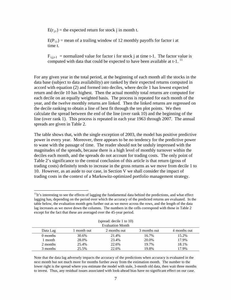
For any given year in the total period, at the beginning of each month all the stocks in the data base (subject to data availability) are ranked by their expected returns computed in accord with equation (2) and formed into deciles, where decile 1 has lowest expected return and decile 10 has highest. Then the actual monthly total returns are computed for each decile on an equally weighted basis. The process is repeated for each month of the year, and the twelve monthly returns are linked. Then the linked returns are regressed on the decile ranking to obtain a line of best fit through the ten plot points. We then calculate the spread between the end of the line (over rank 10) and the beginning of the line (over rank 1). This process is repeated in each year 1963 through 2007. The annual spreads are given in Table 2. The table shows that, with the single exception of 2003, the model has positive predictive power in every year. Moreover, there appears to be no tendency for the predictive power to wane with the passage of time. The reader should not be unduly impressed with the magnitudes of the spreads, because there is a high level of monthly turnover within the deciles each month, and the spreads do not account for trading costs. The only point of Table 2’s significance to the central conclusion of this article is that return (gross of trading costs) definitely tends to increase in the gross returns as we move from decile 1 to 10. However, as an aside to our case, in Section V we shall consider the impact of trading costs in the context of a Markowitz-optimized portfolio management strategy.

11It’s interesting to see the effects of lagging the fundamental data behind the predictions, and what effect lagging has, depending on the period over which the accuracy of the predicted returns are evaluated. In the table below, the evaluation month gets further out as we move across the rows, and the length of the data lag increases as we move down the columns. The numbers in the cells correspond with those in Table 2 except for the fact that these are averaged over the 45-year period.

(spread: decile 1 to 10) Evaluation Month

Data Lag 1 month out 2 months out 3 months out 4 months out 0 months 30.6% 21.4% 16.7% 15.2% 1 month 28.0% 23.4% 20.0% 17.9% 2 months 25.4% 22.6% 19.7% 18.1% 3 months 25.5% 22.6% 19.8% 17.9%

Note that the data lag adversely impacts the accuracy of the predictions when accuracy is evaluated in the next month but not much more for months further away from the estimation month. The number to the lower right is the spread where you estimate the model with stale, 3-month old data, then wait three months to invest. Thus, any residual issues associated with look-ahead bias have no significant effect on our case.

7

Some would argue that the spreads are reflective of differences in risk between the deciles, with decile 10 being more risky and decile 1 less risky. In the next section we investigate these decile characteristics.

IV. Our Case Ends – The Characteristics of Deciles One through Ten Table 3 shows the profile characteristics of the ten deciles. The numbers presented in the table are z-scores (number of standard deviations below or above the mean in a normalized distribution for the population). As we go from decile 1 through decile 10, the transformation in the character of the deciles is absolutely stunning. In terms of the risk associated with returns to the stocks, there can be no doubt that risk decreases as we go from the lowest expected return deciles to the highest. This, of course, is consistent with our findings that the payoff to risk is consistently negative over the 45-year period of this study. The spreads between the extreme deciles are larger for variance of total return and residual risk then they are for market beta, indicating that these may be more important to pricing than beta. We also see that high expected return stocks are larger in terms of market capitalization. The inescapable conclusion here is that higher gross expected return is associated with lower market risk. The picture becomes even more interesting as we move to fundamentals. As we go from decile 1 through decile 10, measures of profitability improve dramatically. High expected return stocks are clearly more profitable. Moreover, looking at the trend in profitability over the trailing 5-year window, the high expected return stocks are becoming even more profitable within this window. A higher fraction of the high expected return stocks also tend to pay dividends. High expected return stocks also sell at cheaper prices relative to earnings, cash flow, book value, and dividends than their low expected return counterparts. The total returns to higher expected return stocks are also larger over the trailing 6 and 12-month periods. Thus, high expected return is associated with trailing momentum in the stock price. In Table 4 we see the differences in the z-scores between deciles 10 and 1 for the whole period and for the five sub-periods. Consistent with our findings on the stability of the t-statistics in Table 1, the characteristics of high and low expected return stocks is amazingly stable over time. The relative nature of the profiles for high and low expected return holds in every period, save for book-to-price in the first sub-period, 6-month return in the second sub-period, and trend in profit margin in the final 5-year period. There can be no question that the high expected return decile has a more attractive profile than the low expected return decile and that this relative attraction continues through the decades.

8

A new type of investment style is being revealed here. Value and growth styles are well known. Some managers also offer a style that is known as “growth at a reasonable price”(GARP), in which they attempt to invest in stocks with good prospects while maintaining discipline in terms of the prices they are willing to pay. Our results reveal that it is possible to go beyond GARP. It is possible to get “growth at a low price”(GALP)12. Individually, the market is sufficiently efficient that few, if any, stocks individually have the GALP profile.13

14

However, it seems that the stock market is sufficiently inefficient that it is possible to assemble a collective portfolio (like our decile 10) that indeed has the GALP profile. It’s as if the market can see, and price, individual profiles but not potential combinations. Let’s assess this evidence with some simple intuition. Look at the nature of the profile of decile 1 – risky, smaller capitalization, lower profitability and getting even worse, selling at relatively high prices compared to earnings, cash flow, sales and dividends, and with negative momentum over the past year. Compare this with the profile of decile 10 – lower risk, larger capitalization, higher profitability and getting even better, selling at low prices relative to earnings, cash flow, sales and dividends, with positive momentum over the past year. Ask yourself the following question. Given a choice between investing in these two profiles, which would you choose? We can safely say that the vast majority of investors would choose decile 10.15 And, as it turns out, in the context of an inefficient market, this is the correct choice. Difficult as it may be to admit, the evidence strongly suggests that this simple intuition is more powerful than any of the complex theories about expected return that can be found in the literature of Modern Finance! The fundamental argument of our case is that there can be no question that risk goes down as you move from decile 1 through 10. In our view lingering discussion will center on whether net (of trading costs) return goes up or down as you move from 1 through 10. As we see in Table 2, in terms of gross return, it obviously goes up. Some may try to argue that the relative magnitude of trading costs required for maintaining high and low risk positions are crucial.16 . Discussions should center on the level of risk aversion 12 This new investment style might be pronounced “gallop”. 13 This raises an issue regarding the procedure by which money managers construct their portfolios. Stylized managers frequently sort stocks on the basis of some measure or measures of cheapness and then evaluate the sorted stocks on the basis of subjective considerations. Sorting procedures, whether applied to growth or value styles are limiting. To construct a GALP portfolio you need to consider how each stock contributes to the profile of the final portfolio, much in the way a chef considers how each ingredient contributes to the taste of the final dish. Rather than sorting, portfolio managers might want to turn to linear programming to create attractive GALP opportunities. 14 As an explanation of why our results have not been revealed in academic studies by others, most studies of properties of the cross-section also use ranking procedures. Ranking procedures again fall short in revealing the surprising characteristics of truly high and low expected return stock portfolios. 15 This assertion is based on an informal survey of many thousands of investors to whom Haugen has raised the issue in many speeches. Of course, until the issue was raised, the vast majority of these investors were never aware of the existence of GALP or its polar opposite DADP (decline at a dear price). 16 Suppose that, in the efficient market, the only determinant of differences in cross-sectional expected return was market beta. As an investor you could invest in the market portfolio, which has a beta of one. This decision would likely require relatively low trading costs. Moving either to a higher or lower beta would require higher portfolio turnover to maintain the investment objective of higher or lower beta. The expected trading costs associated with increasing your personal utility by moving either to the left (lower

9

displayed in the cross-section (net of trading costs) relative to the dramatically high level of risk aversion revealed in our longitudinal analysis as shown immediately below. In Figure 1 we show the relationship between daily changes in the implied volatility17 (the VIX, computed from options on the S&P 500 stock index) and the percentage changes in the index itself. Clearly, as the market’s assessment of risk over the expiration period of the options goes up, the value of the index goes down.18

19

A full 47% of the daily percentage changes in the index can be explained by changes in the market’s assessment of its volatility. As volatility goes up, risk-averse investors require a higher rate of return on their stock investments. Given current expectations of future dividends, they can only get this by lowering the current market value of common stock. Figure 1 reveals a high level of risk aversion on the part of investors. But where is any trace of risk aversion in Table 3? Advocates of the efficient market hypothesis must reconcile Table 2, Table 3, and Figure 1. In our opinion, that is an impossible task. Clearly, the combination of the results presented in Table 2, Table 3, and Figure 1 is a stake through the heart of the efficient market hypothesis. Given the strong results of Figure 1, in order to accept the view of those who think the market is efficient, realized return, net of trading costs, must fall dramatically as you move from 1 to 10. Those, who wish to maximize their utility by taking positions with the characteristics associated with decile 10, must face significantly lower returns, net of trading costs, than those taking positions with the characteristics associated with decile 1. Advocates of the efficient market hypothesis face a daunting task, since positions in the neighborhood of decile 10 will tend to be in larger companies. In our view this “net-return hypothesis” will never be credible. Note that it’s not sufficient to show that a strategy whereby you “go short” decile 1 (and therefore add trading costs to its returns) and “go long” decile 10 (subtracting trading costs from its returns) is unprofitable. Instead, it must be shown that assuming higher (lower) risk garners higher (lower) returns net of the trading costs associated with maintaining and managing these higher (lower) risk positions.20

beta) or to the right (higher beta) should be subtracted from both the expected returns to establish the true relationship between risk and return. 17 In Chapter 11 of Haugen (2009) it is argued that changes in implied volatility mostly stem from the market’s observation and reactions to its own recent pricing behavior, rather than reaction to real economic events. To support this notion, in the Appendix to Chapter 11, it is shown that the largest volatility shifts in Figure 1 aren’t associated with the occurrences of notable real events In this sense the lion’s share of what Haugen calls “price-driven volatility” is attributable to changes in the market’s perception of its risk and its simultaneous reactions to those changes. However, it should be noted that the case presented in this article is unrelated to the validity of the price-driven volatility hypothesis. 18 For those who wish to argue that the causation goes in the opposite direction from the return to implied volatility we would ask, “Why are extreme positive returns associated with reductions in implied volatility while extreme negative returns are associated with increases in implied volatility?” 19 For examples of additional longitudinal evidence of risk aversion see French, Schwert and Stambaugh (1987) and Haugen, Talmor and Torous (1991). 20 It should be noted that while the GALP and DADP styles are a natural consequence of following a comprehensive expected return factor model, investors can move deep into GALP or DADP with simple linear programming algorithms where portfolio turnover is kept at very low levels.

10

We feel that our case against an efficient stock market is proved beyond a shadow of a doubt at this point. However, in the spirit of this volume, in the next section we shall see if these inefficiencies can be exploited after allowing for trading costs using a Markowitz-based investment strategy.

V. The Profitability of Portfolios Managed with the Expected Return Factor Model

Nine years after the publication of our original article, Hanna and Ready (2005) wrote an article in which they replicated, as closely as possible, our original results for the U.S. markets. They then tested a trading strategy whereby deciles 1 and 10 are traded and the difference in returns is considered net of transactions costs. They contend the turnover associated with trading strategies using the expected return factor model eliminates its advantage relative to a strategy based on simple book-to-price or momentum. In Section 8 of our original article, we presented the results of an optimized (using a Markowitz-type procedure) investment strategy that was limited to the 1000 largest U.S. stocks. Portfolio turnover was limited to 20% to 40% per year and trading costs for these largest stocks were assumed to be a very generous 2% per round-trip. We showed that between 1979 and 1993 the difference in annualized return net of transactions costs, between a portfolio, optimized to provide maximum return, and the market index, was approximately 4%. This is what we argued to be the profitable predictability of the model. In Section 10 of our article we provided a similar optimization analysis, net of transactions costs, in several individual countries. In this article we expand our original optimized results to cover the extended time period and the five sub-periods21. In the optimizations, portfolio trading is controlled through a penalty function. When available, the optimizations are based on the largest 1000 stocks in the database. Estimates of portfolio volatility are based on the full covariance matrix of returns to the 1000 stocks in the previous 24 months. Two years of monthly return data, from 1963 through 1964, are used to construct the covariance matrix for the initial portfolios. Estimates of expected returns to the 1000 stocks are based on the expected return factor model discussed above. The following constraints are applied to portfolio weights for each quarterly optimization:

(1) The maximum weight in a portfolio that can be assigned to a single stock is limited to 5%. The minimum is 0% (Short selling is not permitted).

(2) The maximum invested in any one stock in the portfolio is three times the market capitalization weight or 0.25%, whichever is greater, subject to the 5% limit. (subject to the 5% limit in the first constraint)

21 We don’t account for a 1-day trading lag in our analysis as did Hanna and Ready. This is because those who use the expected return factor model in practice re-estimate the model as of the close of trading at the end of the month, work into the evening, and then rebalance their positions at the opening bell.

11

(3) The portfolio industry weight is restricted to be within 3% of the market capitalization weight of that industry. (Based on the two-digit SIC code.)

(4) Turnover in the portfolio is penalized through a linear cost applied to the trading of each stock. As a simplification, all stocks are subject to the same linear turnover cost although in practice portfolio managers use differential trading costs in their optimizations.

These constraints are designed to merely keep the portfolios diversified. Reasonable changes in the constraints do not materially affect the results. As in our original article, the portfolios are re-optimized quarterly. 22 The performances of the four optimized portfolios across the total period and the sub-periods are presented in Figures 2a through 2f and in Table 6. In the figures the dots represent the four optimized portfolios. The triangle shows the position of the market benchmark. In the optimization process we attempt to create a global minimum variance portfolio (which doesn’t employ the expected return factor model at all) and three portfolios (that do employ the model) that aim for successively higher expected return while minimizing volatility. Trading costs are not reflected in Figures 2a through 2f. We leave to the reader’s judgment what the trading costs might be. However, in Table 5 we present the average annual turnover for each of the portfolios. To calculate what the round-trip trading cost would be, in order to eliminate the spread between an optimized portfolio and the benchmark, simply divide the spread by the average annual turnover. Obviously, transactions costs would have to be unrealistically extreme to significantly close the gap between the high expected return portfolios and the market index. Results for the optimizations in the sub-periods are presented in Figures 2b through 2f. Note the positions of the benchmark23 relative to the global minimum variance portfolios. The positions reflect the fact that the cross-sectional payoff to risk was negative during the 45-year period. If we had constructed equally weighted portfolirandomly selected stocks, and plotted their realized return against their volatility, our imagined scatter plot would have had a negative slope in the fig 24

os of

ures.

VI. Summary

We find that measures of current profitability and cheapness are highly significant in determining the structure of the cross-section of stock returns. The statistical significance

22 With unconstrained optimization, with 24 monthly observations and 1000 stocks, there is no unique solution. However, given the constraints provided above, unique solutions exist. 23 The benchmark is the Russell 1000 stock index for as long as it was in existence. Prior to that the benchmark is the S&P 500 stock index. 24 This is essentially what Haugen and Heins found in 1969.

12

of risk is also high, but the payoff to risk has the wrong sign period after period. The riskiest stocks over measures including market beta, total return variance, and residual volatility tend to have the lowest returns. We also find that 1-year momentum pays off positively, and that last month’s residual return and last quarters total return pays off negatively. As in our earlier article the comprehensive expected return factor model is very powerful in predicting the future relative returns on stocks. High-return stock decile composites tend to be relatively large companies with low risk and they have positive market price momentum. The profitability of high-return stocks is good and getting better. The low-return counterparts to these stocks have the opposite profile. Rational investors would likely find the high-return profile very attractive and the low-return profile very scary. Subsequently, they would tend to find their intuition about future return to have been proven correct. While high expected return deciles tend to be unambiguously less risky, we find strong evidence supporting a high level of risk aversion in longitudinal data. This doesn’t square at all with the cross-sectional evidence of risk loving, unless the traces of risk aversion in the cross-section have been grossly distorted by mispricing within the cross-section.

In tests of rational trading strategies, where we can account for trading costs, the expected return factor model appears to be profitable net of reasonable trading costs. Profitability issues related to this section are irrelevant to our case against stock market efficiency. However, our case stands, aside from issues of profitability.

Although attempts may be made, it’s not likely that these results can be overturned without employing outrageous assumptions regarding investor risk preferences, convoluted econometric techniques, or self-serving, multi-factor “risk adjustment procedures”. The results presented here are the product of irrational behavior and the complexity and uniqueness of the interactions on the part of investors. Like it or not, these results are out there for all to find and to understand.

Given the overwhelming evidence presented here, the following conclusions are undeniable:

• The cross-sectional payoff to risk bearing is highly negative.

• The longitudinal payoff to risk bearing is highly positive.

• The safest and most attractive stock portfolios have the highest expected

returns.

• The scariest stock portfolios have the lowest expected returns.

13

An efficient market doesn’t simultaneously exhibit strong levels of risk loving in the cross-section and strong levels of risk aversion in the aggregate.

Case closed.

Note: Effective 4/15/09, if you have comments about this paper, please go to:

http://www.caseclosed.ws/

14

Bibliography

Ang, Abdrew, Robert J. Hodrick, Yuhang Xing, and Xiaoyan Zhang, 2006, The Cross-section of Volatility and Expected Returns, The Journal of Finance, 259-299. Fama, Eugene F. and Kenneth R. French, 1992, The Cross-section of Expected Stock Returns, Journal of Finance, 427-465. Fama, Eugene F. and Kenneth R. French, 2008, Dissecting Anomalies, Journal of Finance, 1653-1678. Fama, Eugene F. and James MacBeth, 1973, Risk, Return and Equilibrium: Empirical Tests, Journal of Political Economy, 607-636. French, Kenneth R., William Schwert and Robert Stambaugh, 1987, Expected Stock Returns and Volatility, Journal of Financial Economics, 3-29. Hanna, J. Douglas and Mark J. Ready, 2005, Profitable Predictability in the Cross Section of Stock Returns, Journal of Financial Economics, 463-505. Haugen, Robert A., The Inefficient Stock Market—Second Edition (Prentice Hall, Upper Saddle River, New Jersey, 2002) Haugen, Robert A. The New Finance – Overreaction, Complexity and Uniqueness, Third Edition, (Prentice Hall, Upper Saddle River, New Jersey, 2004) Haugen, Robert A. The New Finance – Overreaction, Complexity and Their Consequences, Fourth Edition, (Prentice Hall, Upper Saddle River, New Jersey, 2009, forthcoming) Haugen, Robert A. and A. James Heins, 1975, Risk and the Rate of Return on Financial Assets: Some Old Wine in New Bottles, Journal of Financial and Quantitative Analysis, 775-784. Haugen, Robert A. and Nardin L. Baker, 1996, Commonality in the Determinants of Expected Stock Returns, Journal of Financial Economics, 401-439. Haugen, Robert A., Eli Talmor and Walter Torous, 1991, The Effect of Volatility Changes on the Level of Stock Prices and Subsequent Expected Return, The Journal of Finance, 985-1007. Jegadeesh, Narasimhan and Sheridan Titman, 1993, Returns to Buying Winners and Selling Losers: Implications for Stock Market Efficiency, The Journal of Finance,65-92.

15

Lettau, Martin and Jessica A. Wachter, 2007, Why is the Long-horizon Equity Less Risky? A Duration-based Explanation of the Value Premium, The Journal of Finance, 55-92.

16

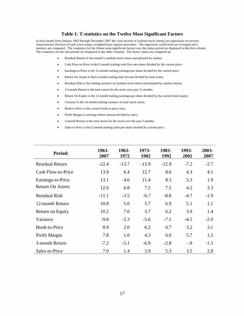
Table 1: T-statistics on the Twelve Most Significant Factors In each month from January 1963 through December 2007 the cross-section of realized stock returns are regressions on seventy characteristics (factors) of each stock using a weighted least squares procedure. The regression coefficients are averaged and t-statistics are computed. The t-statistics for the fifteen most significant factors over the entire period are displayed in the first column. The t-statistics for the sub-periods are displayed in the other columns. The factor values are computed as:

• Residual Return is last month’s residual stock return unexplained by market.

• Cash Flow-to-Price is the12-month trailing cash flow-per-share divided by the current price.

• Earnings-to-Price is the 12-month trailing earnings-per-share divided by the current price.

• Return On Assets is the12-month trailing total income divided by total assets.

• Residual Risk is the trailing variance of residual stock return unexplained by market return).

• 12-month Return is the total return for the stock over past 12 months.

• Return On Equity is the 12-month trailing earnings-per-share divided by the current book equity.

• Variance is the 24-month trailing variance of total stock return.

• Book-to-Price is the current book-to-price ratio.

• Profit Margin is earnings before interest divided by sales.

• 3-month Return is the total return for the stock over the past 3 months.

• Sales-to-Price is the12-month trailing sales-per-share divided by current price.

Period: 1963-2007

1963-1972

1973-1982

1983-1992

1993-2002

2003-2007

Residual Return -22.4 -13.7 -15.9 -12.9 -7.2 -2.7

Cash Flow-to-Price 13.9 6.4 12.7 8.6 4.3 4.1

Earnings-to-Price 13.1 4.0 11.4 8.3 5.3 1.9Return On Assets 12.6 6.8 7.5 7.5 4.2 3.3

Residual Risk -11.1 -3.5 -6.7 -8.8 -4.7 -1.9

12-month Return 10.8 5.0 5.7 6.9 5.1 1.1

Return on Equity 10.2 7.0 3.7 6.2 3.9 1.4

Variance -9.0 -2.3 -5.6 -7.1 -4.5 -2.0

Book-to-Price 8.9 2.0 6.2 6.7 3.2 3.1

Profit Margin 7.8 1.0 4.3 6.0 5.7 1.5

3-month Return -7.2 -5.1 -6.9 -2.8 -.9 -1.5

Sales-to-Price 7.0 1.4 3.9 5.3 3.5 2.8

17

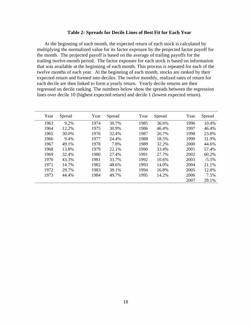
Table 2: Spreads for Decile Lines of Best Fit for Each Year

At the beginning of each month, the expected return of each stock is calculated by multiplying the normalized value for its factor exposure by the projected factor payoff for the month. The projected payoff is based on the average of trailing payoffs for the trailing twelve-month period. The factor exposure for each stock is based on information that was available at the beginning of each month. This process is repeated for each of the twelve months of each year. At the beginning of each month, stocks are ranked by their expected return and formed into deciles. The twelve monthly, realized rates of return for each decile are then linked to form a yearly return. Yearly decile returns are then regressed on decile ranking. The numbers below show the spreads between the regression lines over decile 10 (highest expected return) and decile 1 (lowest expected return).

Year Spread Year Spread Year Spread Year Spread 1963 9.2% 1974 30.7% 1985 36.6% 1996 10.4%1964 12.2% 1975 30.9% 1986 46.4% 1997 46.4%1965 30.0% 1976 32.4% 1987 26.7% 1998 23.8%1966 9.4% 1977 24.4% 1988 18.5% 1999 31.9%1967 49.1% 1978 7.8% 1989 32.2% 2000 44.6%1968 13.8% 1979 22.1% 1990 33.4% 2001 57.4%1969 32.4% 1980 27.4% 1991 27.7% 2002 60.2%1970 43.3% 1981 33.7% 1992 10.6% 2003 -5.5%1971 14.7% 1982 48.6% 1993 14.0% 2004 21.1%1972 29.7% 1983 39.1% 1994 16.8% 2005 12.8%1973 44.4% 1984 49.7% 1995 14.2% 2006 7.5%

2007 29.1%

18

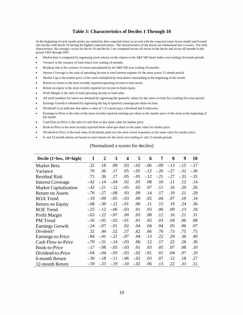
Table 3: Characteristics of Deciles 1 Through 10

At the beginning of each month stocks are ranked by their expected return in accord with the expected return factor model and formed into deciles with decile 10 having the highest expected return. The characteristics of the stocks are normalized into z-scores. For each characteristic, the average z-score for decile 10 and decile 1 are computed across all stocks in the decile and across all months in the period 1963 through 2007. • Market beta is computed by regressing stock returns on the returns to the S&P 500 Stock Index over trailing 24-month periods. • Variance is the variance of total return over trailing 24-months. • Residual risk is the variance of return unexplained by the S&P 500 over trailing 24-months. • Interest Coverage is the ratio of operating income to total interest expense for the most recent 12-month period. • Market Cap is the market price of the stock multiplied by total shares outstanding at the beginning of the month. • Return on Assets is the most recently reported operating income to total assets. • Return on equity is the most recently reported net income to book equity. • Profit Margin is the ratio of total operating income to total sales. • All trend numbers for ratios are obtained by regressing the quarterly values for the ratios on time for a trailing five-year period. • Earnings Growth is obtained by regressing the log of quarterly earnings-per-share on time. • Dividend? is an indicator that takes a value of 1 if a stock pays a dividend and 0 otherwise. • Earnings-to-Price is the ratio of the most recently reported earnings-per-share to the market price of the stock at the beginning of

the month. • Cash Flow-to-Price is the ratio of cash flow to this same value for market price. • Book-to-Price is the most recently reported book value-per-share to the same value for market price. • Dividend-to-Price is the total value of dividends paid over the most recent 4-quarters to the same value for market price. • 6- and 12-month returns are based on total returns for the stock over trailing 6- and 12-month periods.

(Normalized z-scores for deciles)

Decile (1=low, 10=high) 1 2 3 4 5 6 7 8 9 10Market Beta .32 .18 .09 .03 -.02 -.06 -.09 -.13 -.15 -.17Variance .70 .36 .17 .05 -.05 -.12 -.20 -.27 -.32 -.36Residual Risk .71 .36 .17 .05 -.05 -.12 -.21 -.27 -.33 -.35Interest Coverage -.42 -.14 -.04 .02 .05 .08 .10 .11 .12 .14Market Capitalization -.42 -.21 -.12 -.05 .02 .07 .11 .16 .20 .26Return on Assets -.76 -.27 -.08 .03 .09 .14 .17 .19 .21 .29ROA Trend -.19 -.09 -.05 -.03 .00 .02 .04 .07 .10 .14Return on Equity -.68 -.30 -.12 -.01 .06 .11 .15 .19 .24 .36ROE Trend -.25 -.12 -.06 -.03 .01 .03 .06 .09 .13 .18Profit Margin -.63 -.22 -.07 .00 .05 .08 .12 .16 .21 .31PM Trend -.16 -.05 -.02 -.01 .01 .02 .03 .04 .06 .08Earnings Growth -.24 -.07 -.01 .02 .04 .04 .04 .05 .06 .07Dividend? .32 .44 .52 .57 .62 .66 .70 .73 .75 .75Earnings-to-Price -.84 -.41 -.21 -.07 .04 .13 .22 .29 .36 .49Cash Flow-to-Price -.70 -.31 -.14 -.03 .06 .12 .17 .22 .26 .36Book-to-Price -.17 -.08 -.05 -.03 .01 .03 .05 .07 .08 .10Dividend-to-Price -.04 -.04 -.03 -.03 -.02 -.01 .01 .04 .07 .106-month Return -.30 -.18 -.11 -.06 -.02 .03 .07 .12 .18 .2712-month Return -.59 -.33 -.19 -.10 -.02 .06 .13 .22 .33 .51

19

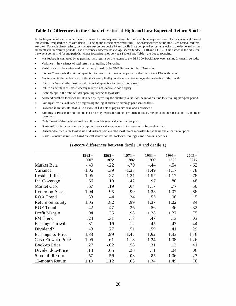
Table 4: Differences in the Characteristics of High and Low Expected Return Stocks

At the beginning of each month stocks are ranked by their expected return in accord with the expected return factor model and formed into equally-weighted deciles with decile 10 having the highest expected return. The characteristics of the stocks are normalized into z-scores. For each characteristic, the average z-score for decile 10 and decile 1 are computed across all stocks in the decile and across all months in the various periods. The differences between the average scores for deciles 10 and 1 (10 – 1) are shown in the table for the whole period and for sub-periods. Minor inconsistencies between Table 3 and Table 4 are due to rounding. • Market beta is computed by regressing stock returns on the returns to the S&P 500 Stock Index over trailing 24-month periods. • Variance is the variance of total return over trailing 24-months. • Residual risk is the variance of return unexplained by the S&P 500 over trailing 24-months. • Interest Coverage is the ratio of operating income to total interest expense for the most recent 12-month period. • Market Cap is the market price of the stock multiplied by total shares outstanding at the beginning of the month. • Return on Assets is the most recently reported operating income to total assets. • Return on equity is the most recently reported net income to book equity. • Profit Margin is the ratio of total operating income to total sales. • All trend numbers for ratios are obtained by regressing the quarterly values for the ratios on time for a trailing five-year period. • Earnings Growth is obtained by regressing the log of quarterly earnings-per-share on time. • Dividend is an indicator that takes a value of 1 if a stock pays a dividend and 0 otherwise. • Earnings-to-Price is the ratio of the most recently reported earnings-per-share to the market price of the stock at the beginning of

the month. • Cash Flow-to-Price is the ratio of cash flow to this same value for market price. • Book-to-Price is the most recently reported book value-per-share to the same value for market price. • Dividend-to-Price is the total value of dividends paid over the most recent 4-quarters to the same value for market price. • 6- and 12-month returns are based on total returns for the stock over trailing 6- and 12-month periods.

(z-score differences between decile 10 and decile 1)

1963 –

2007 1963 –

1972 1973 –

1982 1983 –

1992 1993 –

1902 2003 –

2007 Market Beta -.49 -.22 -.70 -.44 -.54 -.62Variance -1.06 -.39 -1.33 -1.49 -1.17 -.78Residual Risk -1.06 -.37 -1.31 -1.57 -1.17 -.78Int. Coverage .56 .10 .42 .97 .80 .48Market Cap. .67 .19 .64 1.17 .77 .50Return on Assets 1.04 .95 .90 1.33 1.07 .88ROA Trend .33 .44 .34 .53 .08 .15Return on Equity 1.05 .82 .89 1.37 1.22 .84ROE Trend .42 .47 .36 .56 .36 .32Profit Margin .94 .35 .98 1.28 1.27 .75PM Trend .24 .31 .18 .47 .13 -.03Earnings Growth .31 .16 .12 .45 .43 .44Dividend? .43 .27 .51 .59 .41 .29Earnings-to-Price 1.33 .99 1.47 1.62 1.33 1.16Cash Flow-to-Price 1.05 .61 1.18 1.24 1.08 1.26Book-to Price .27 -.02 .58 .31 .13 .41Dividend-to-Price .14 .05 .38 .11 .04 .066-month Return .57 .56 -.03 .85 1.06 .2712-month Return 1.10 1.12 .63 1.34 1.49 .76

20

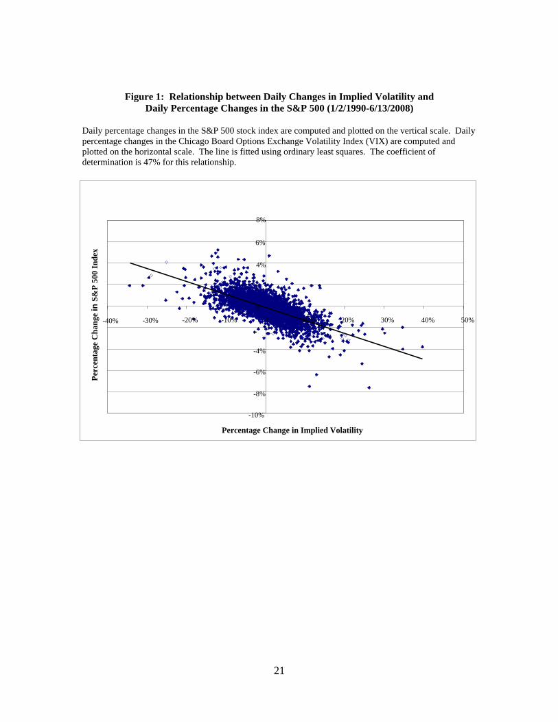
Figure 1: Relationship between Daily Changes in Implied Volatility and Daily Percentage Changes in the S&P 500 (1/2/1990-6/13/2008)

Daily percentage changes in the S&P 500 stock index are computed and plotted on the vertical scale. Daily percentage changes in the Chicago Board Options Exchange Volatility Index (VIX) are computed and plotted on the horizontal scale. The line is fitted using ordinary least squares. The coefficient of determination is 47% for this relationship.

-10%

-8%

-6%

-4%

-

0

2

4%

6%

8%

-40% -20% -10% 0 10% 20% 30% 40% 50%

Percentage Change in Implied Volatility

Perc

enta

ge C

hang

e in

S&

P 50

0 In

dex

-30%

21

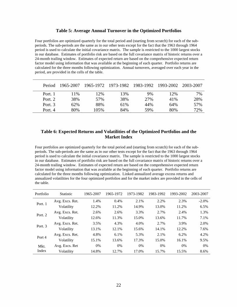
Table 5: Average Annual Turnover in the Optimized Portfolios

Four portfolios are optimized quarterly for the total period and (starting from scratch) for each of the sub-periods. The sub-periods are the same as in our other tests except for the fact that the 1963 through 1964 period is used to calculate the initial covariance matrix. The sample is restricted to the 1000 largest stocks in our database. Estimates of portfolio risk are based on the full covariance matrix of historic returns over a 24-month trailing window. Estimates of expected return are based on the comprehensive expected return factor model using information that was available at the beginning of each quarter. Portfolio returns are calculated for the three months following optimization. Annual turnovers, averaged over each year in the period, are provided in the cells of the table.

Period 1965-2007 1965-1972 1973-1982 1983-1992 1993-2002 2003-2007

Port. 1 11% 12% 13% 9% 12% 7%Port. 2 38% 57% 38% 27% 41% 28%Port. 3 62% 88% 61% 44% 64% 57%Port. 4 80% 105% 84% 59% 80% 72%

Table 6: Expected Returns and Volatilities of the Optimized Portfolios and the Market Index

Four portfolios are optimized quarterly for the total period and (starting from scratch) for each of the sub-periods. The sub-periods are the same as in our other tests except for the fact that the 1963 through 1964 period is used to calculate the initial covariance matrix. The sample is restricted to the 1000 largest stocks in our database. Estimates of portfolio risk are based on the full covariance matrix of historic returns over a 24-month trailing window. Estimates of expected return are based on the comprehensive expected return factor model using information that was available at the beginning of each quarter. Portfolio returns are calculated for the three months following optimization. Linked annualized average excess returns and annualized volatilities for the four optimized portfolios and for the market index are provided in the cells of the table.

Portfolio Statistic 1965-2007 1965-1972 1973-1982 1983-1992 1993-2002 2003-2007

Port. 1 Avg. Excs. Ret. 1.4% 0.4% 2.1% 2.2% 2.3% -2.0%

Volatility 12.2% 11.2% 14.9% 13.0% 11.2% 6.5%

Port. 2 Avg. Excs. Ret. 2.6% 2.6% 3.3% 2.7% 2.4% 1.3%

Volatility 12.6% 11.3% 15.0% 13.6% 11.7% 7.1%

Port. 3 Avg. Excs. Ret. 3.5% 4.3% 4.0% 2.7% 3.9% 2.0%

Volatility 13.1% 12.1% 15.6% 14.1% 12.2% 7.6%

Port 4 Avg. Excs. Ret. 4.8% 6.1% 5.3% 2.1% 6.2% 4.2%

Volatility 15.1% 13.6% 17.3% 15.0% 16.1% 9.5% Mkt. Index

Avg. Excs. Ret 0% 0% 0% 0% 0% 0% Volatility 14.8% 12.7% 17.0% 15.7% 15.5% 8.6%

22

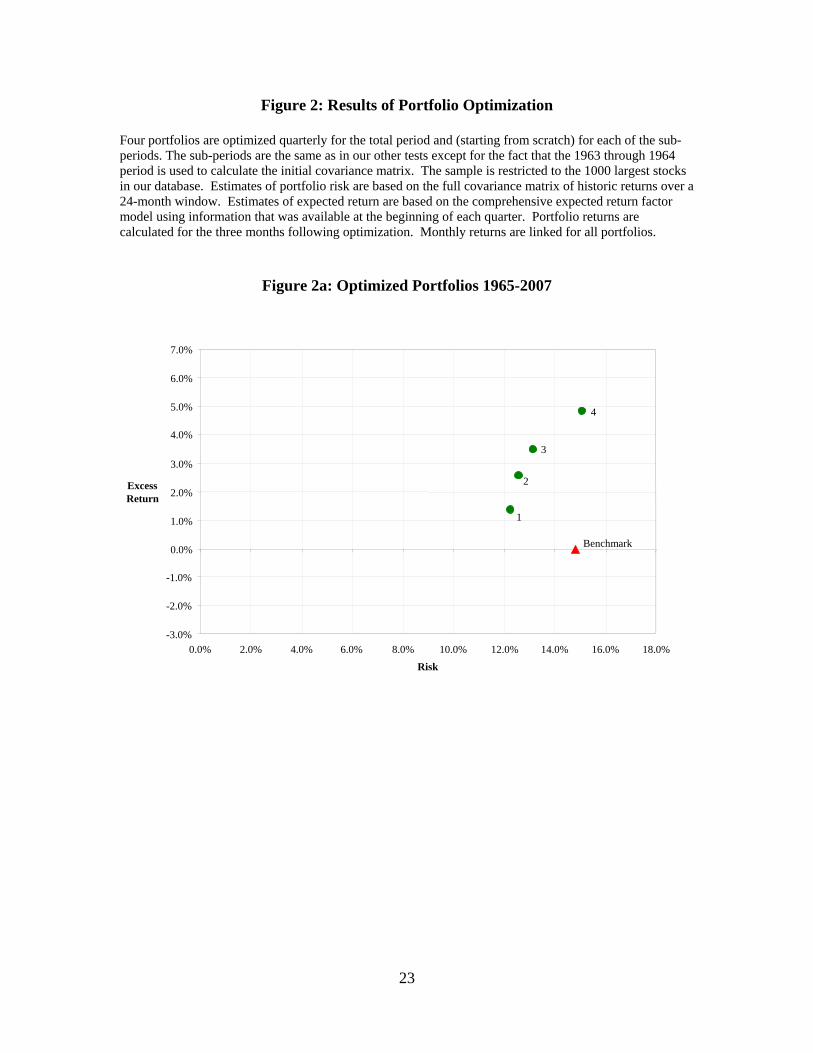
Figure 2: Results of Portfolio Optimization Four portfolios are optimized quarterly for the total period and (starting from scratch) for each of the sub-periods. The sub-periods are the same as in our other tests except for the fact that the 1963 through 1964 period is used to calculate the initial covariance matrix. The sample is restricted to the 1000 largest stocks in our database. Estimates of portfolio risk are based on the full covariance matrix of historic returns over a 24-month window. Estimates of expected return are based on the comprehensive expected return factor model using information that was available at the beginning of each quarter. Portfolio returns are calculated for the three months following optimization. Monthly returns are linked for all portfolios.

Figure 2a: Optimized Portfolios 1965-2007

Benchmark

1

2

3

4

-3.0%

-2.0%

-1.0%

0.0%

1.0%

2.0%

3.0%

4.0%

5.0%

6.0%

7.0%

0.0% 2.0% 4.0% 6.0% 8.0% 10.0% 12.0% 14.0% 16.0% 18.0%Risk

Excess Return

23

Figure 2b: Optimized Portfolios 1965-1972

Benchmark 1

2

3

4

-3.0%

-2.0%

-1.0%

0.0%

1.0%

2.0%

3.0%

4.0%

5.0%

6.0%

7.0%

0.0% 2.0% 4.0% 6.0% 8.0% 10.0% 12.0% 14.0% 16.0% 18.0%

Risk

Excess Return

Figure 2c: Optimized Portfolios 1973-1982

Benchmark

1

2

3

4

-3.0%

-2.0%

-1.0%

0.0%

1.0%

2.0%

3.0%

4.0%

5.0%

6.0%

7.0%

0.0% 2.0% 4.0% 6.0% 8.0% 10.0% 12.0% 14.0% 16.0% 18.0%

Risk

Excess Return

24

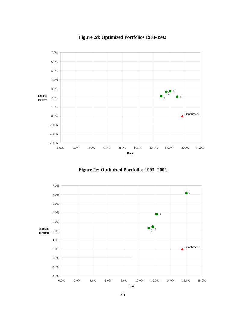
Figure 2d: Optimized Portfolios 1983-1992

Benchmark

12

3 4

-3.0%

-2.0%

-1.0%

0.0%

1.0%

2.0%

3.0%

4.0%

5.0%

6.0%

7.0%

0.0% 2.0% 4.0% 6.0% 8.0% 10.0% 12.0% 14.0% 16.0% 18.0%

Risk

Excess Return

Figure 2e: Optimized Portfolios 1993 -2002

4

3

21

Benchmark

-2.0%

-3.0%

-1.0%

0.0%

1.0%

2.0%

3.0%

4.0%

5.0%

6.0%

7.0%

0.0% 2.0% 4.0% 6.0% 8.0% 10.0% 12.0% 14.0% 16.0% 18.0%

Risk

Excess Return

25

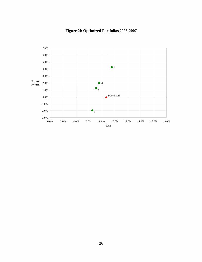
Figure 2f: Optimized Portfolios 2003-2007

4

3

2

Benchmark

-2.0% 1

-3.0%

-1.0%

0.0%

1.0%

2.0%

3.0%

4.0%

5.0%

6.0%

7.0%

0.0% 2.0% 4.0% 6.0% 8.0% 10.0% 12.0% 14.0% 16.0% 18.0%Risk

Excess Return

26