Embed Size (px)
Citation preview

Bayesian Machine Learning
Roadmap:— What is Machine Learning?
— Why/when Bayesian ML?
— Bayesian Interpolation
— Model complexity
Iain MurraySchool of Informatics, University of Edinburgh

What is Machine Learning?
(Depends who you ask)
“Getting computers to use data
to perform better at a task.”
Applications:
— Pattern Recognition, e.g., classification
— Inferring processes underlying data
— Controllers
· · ·

Face detection
How would you detect a face?
(R. Vaillant, C. Monrocq and Y. LeCun, 1994)
http://demo.pittpatt.com/
How does album software
tag your friends?
Face detection
Taken from: http://v10.ahprojects.com/art/cv-dazzle

How do humans do it?
Taken from: http://v10.ahprojects.com/art/cv-dazzle

Response surface optimization
Consult on making a new:concrete, weld, . . . widget?
(antmoose on Flickr, cc-by-2.0)(Bhadeshia et al.)
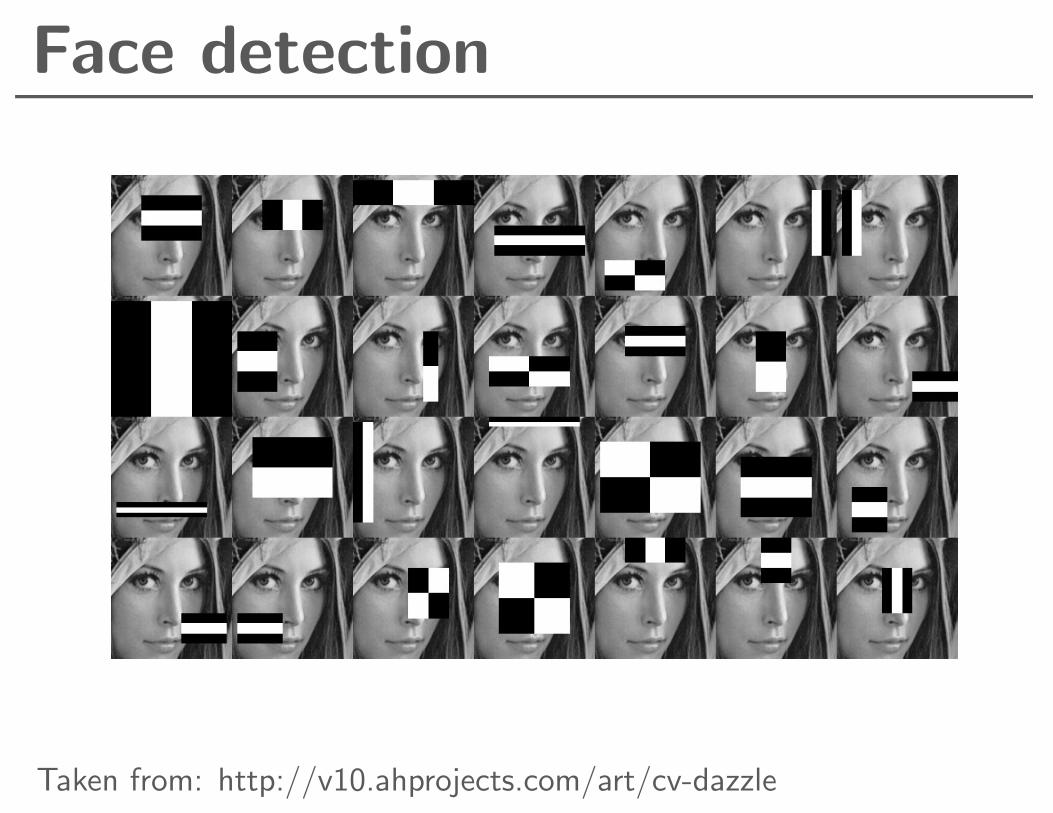
Bayesian Machine learning (examples)
Can be uncertain, even with lots of data:
Bayesian neural networks (MacKay 1995; Neal, 1996)
Bayesian Sets (Ghahramani and Heller, 2006)
TrueSkill (Herbrich, Minka and Graepel, 2006)
Bayesian Matrix Factorization (Salakhutdinov and Mnih, 2008)
...
Often only indirect or limited data about what you’re interested in at any given time.
Overview
Machine learning: fit a bunch of numbers from data
Bayesian: optimal inference with limited information
How much human tweaking is required?
Can our machines have insight?
This lecture: Bayesian interpolation

Linear regression
Elements of Statistical Learning (2nd Ed.) c©Hastie, Tibshirani & Friedman 2009 Chap 3
•• •
••
• ••
•
• •
••
•
•
•
••
•
••
••
•
•
••
•
•• ••
•
•
•
•
•
• ••
•
•
•
•
•
•
•
•
•
•
•• •
•
•
•
••
•
• ••
• •
••
• •••
•
•
•
•
X1
X2
Y
FIGURE 3.1. Linear least squares fitting withX ∈ IR2. We seek the linear function of X that mini-mizes the sum of squared residuals from Y .
Find linear function
y = Xw
that minimizes sum
of squared residuals
from y.
Matlab/Octave:
ww = X \ yy
Elements of Statistical Learning (2nd Ed.) c© Hastie, Tibshirani & Friedman 2009
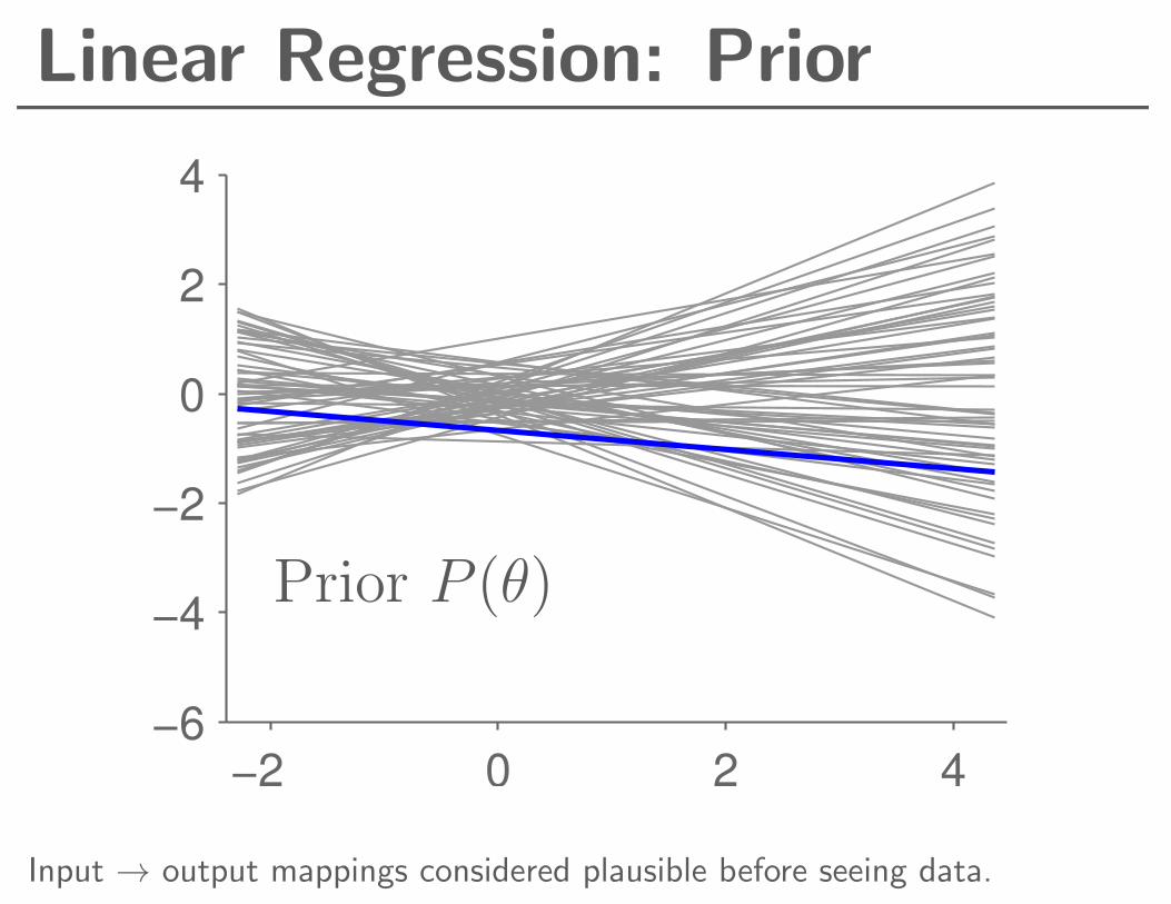
Linear Regression: Prior
−2 0 2 4
−6
−4
−2
0
2
4
Prior P (θ)
Input → output mappings considered plausible before seeing data.
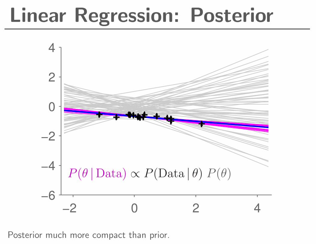
Linear Regression: Posterior
−2 0 2 4
−6
−4
−2
0
2
4
P (θ |Data) ∝ P (Data | θ) P (θ)
Posterior much more compact than prior.
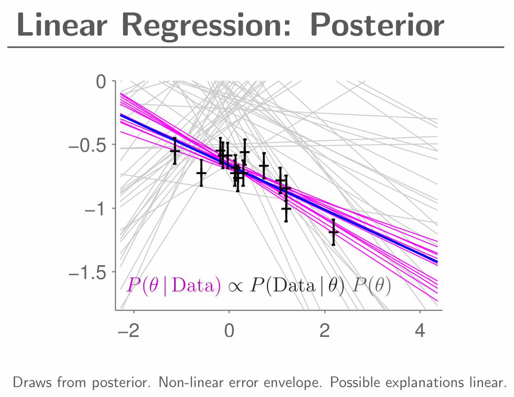
Linear Regression: Posterior
−2 0 2 4
−1.5
−1
−0.5
0
P (θ |Data) ∝ P (Data | θ) P (θ)
Draws from posterior. Non-linear error envelope. Possible explanations linear.
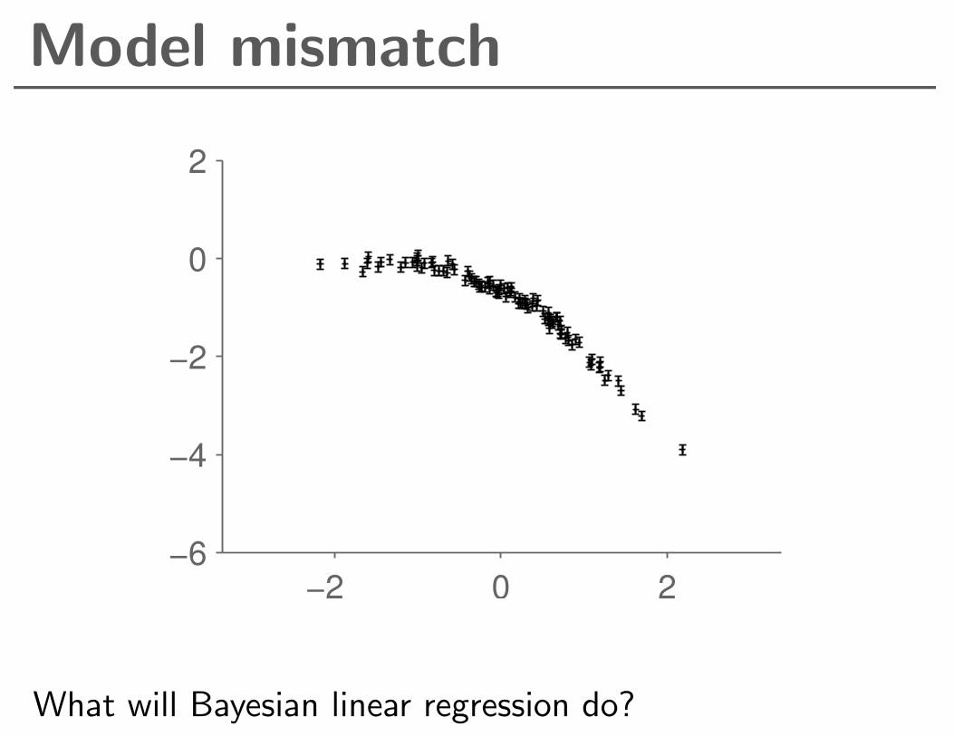
Model mismatch
−2 0 2
−6
−4
−2
0
2
What will Bayesian linear regression do?
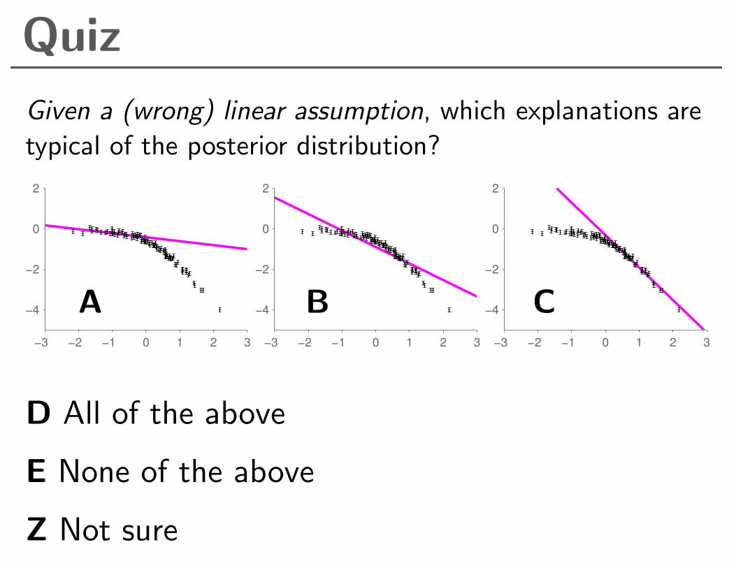
Quiz
Given a (wrong) linear assumption, which explanations are
typical of the posterior distribution?
−3 −2 −1 0 1 2 3
−4
−2
0
2
−3 −2 −1 0 1 2 3
−4
−2
0
2
−3 −2 −1 0 1 2 3
−4
−2
0
2
A B C
D All of the above
E None of the above
Z Not sure
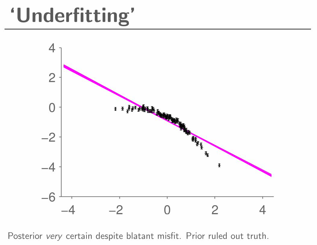
‘Underfitting’
−4 −2 0 2 4
−6
−4
−2
0
2
4
Posterior very certain despite blatant misfit. Prior ruled out truth.
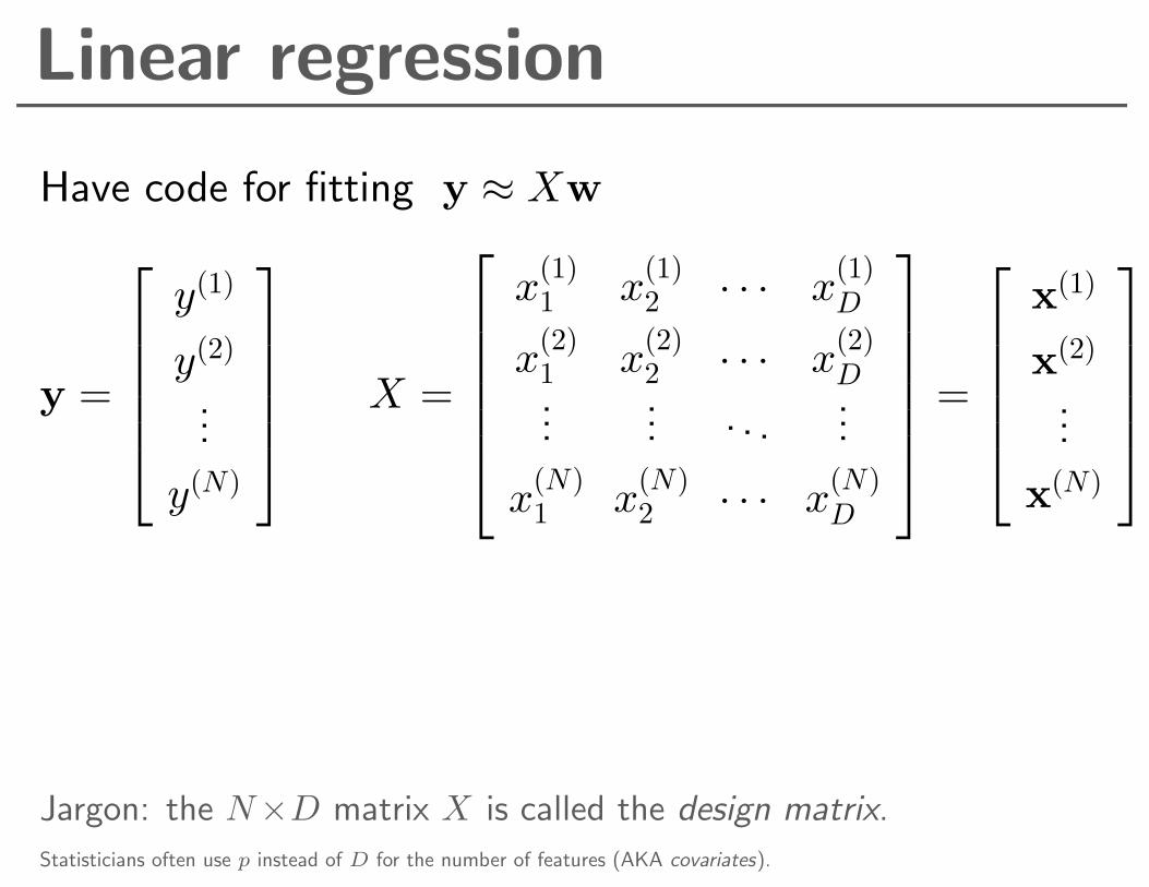
Linear regression
Have code for fitting y ≈ Xw
y =
y(1)
y(2)
...
y(N)
X =
x
(1)1 x
(1)2 · · · x
(1)D
x(2)1 x
(2)2 · · · x
(2)D
...... . . .
...
x(N)1 x
(N)2 · · · x
(N)D
=
x(1)
x(2)
...
x(N)
Jargon: the N×D matrix X is called the design matrix.
Statisticians often use p instead of D for the number of features (AKA covariates).

Linear regression (with features)
y ≈ w1 + w2 x+ w3 x2 = φ(x) ·w or y ≈ Xw:
y =
y(1)
y(2)
...
y(N)
X =
1 x(1) (x(1))2
1 x(2) (x(2))2
......
...
1 x(N) (x(N))2
=
φ(x(1))
φ(x(2))...
φ(x(N))
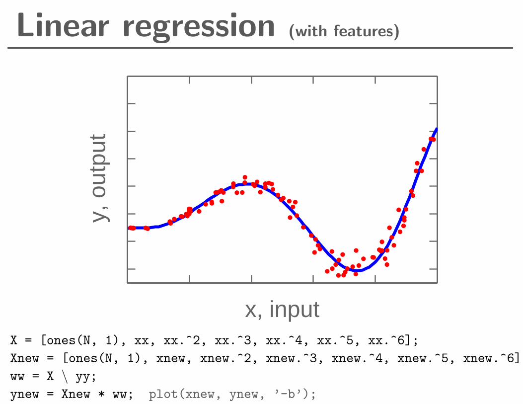
Linear regression (with features)
x, input
y, o
utpu
t
X = [ones(N, 1), xx, xx.^2, xx.^3, xx.^4, xx.^5, xx.^6];
Xnew = [ones(N, 1), xnew, xnew.^2, xnew.^3, xnew.^4, xnew.^5, xnew.^6];
ww = X \ yy;
ynew = Xnew * ww; plot(xnew, ynew, ’-b’);

Overfitting
x, input
y, outp
ut
valid.
p=2
p=5
p=9
train
X = [x.^0, x.^1, x.^2, ..., x.^p];
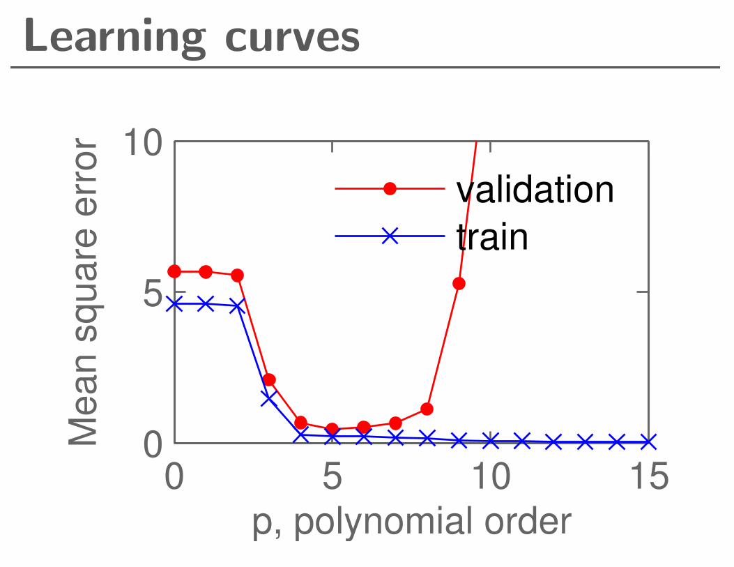
Learning curves
0 5 10 150
5
10
p, polynomial order
Me
an
sq
ua
re e
rro
r
validation
train
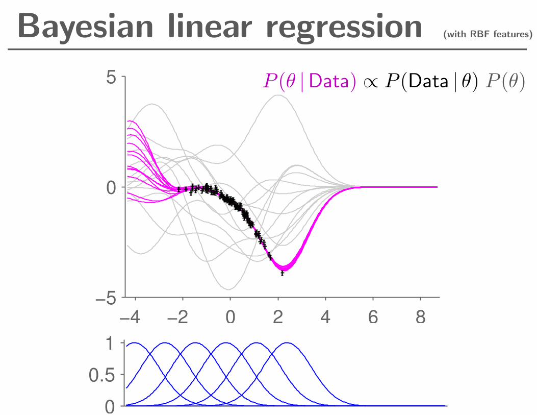
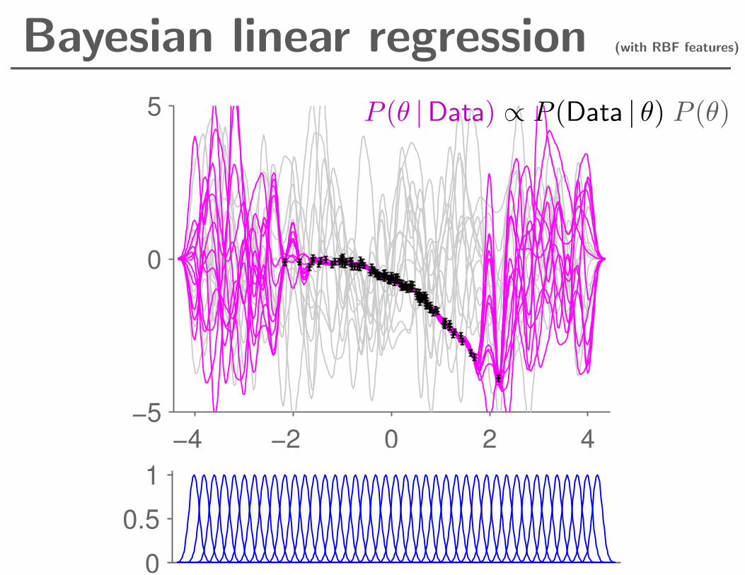
Bayesian linear regression (with RBF features)
−4 −2 0 2 4 6 8
−5
0
5
0
0.5
1
P (θ |Data) ∝ P (Data | θ) P (θ)

Bayesian linear regression (with RBF features)
−4 −2 0 2 4 6 8
−5
0
5
0
0.5
1
P (θ |Data) ∝ P (Data | θ) P (θ)
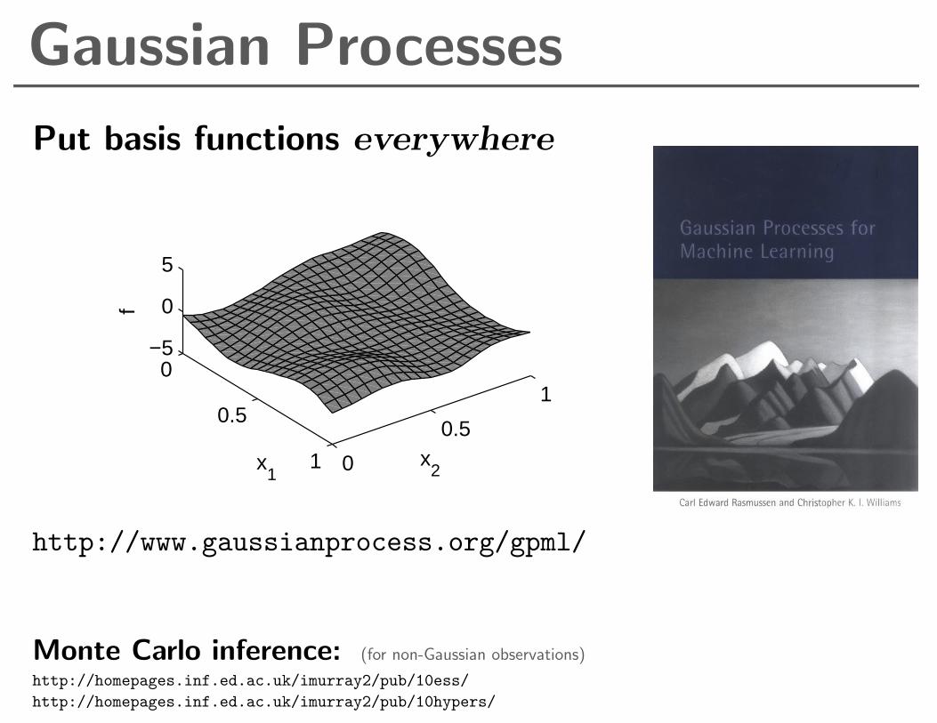
Gaussian Processes
Put basis functions everywhere
0
0.5
1 0
0.5
1
−5
0
5
x2x
1
f
http://www.gaussianprocess.org/gpml/
Monte Carlo inference: (for non-Gaussian observations)
http://homepages.inf.ed.ac.uk/imurray2/pub/10ess/
http://homepages.inf.ed.ac.uk/imurray2/pub/10hypers/

Overview
Bad to rule out truth in prior
Can use large models with little data
Q. What about Occam’s razor?
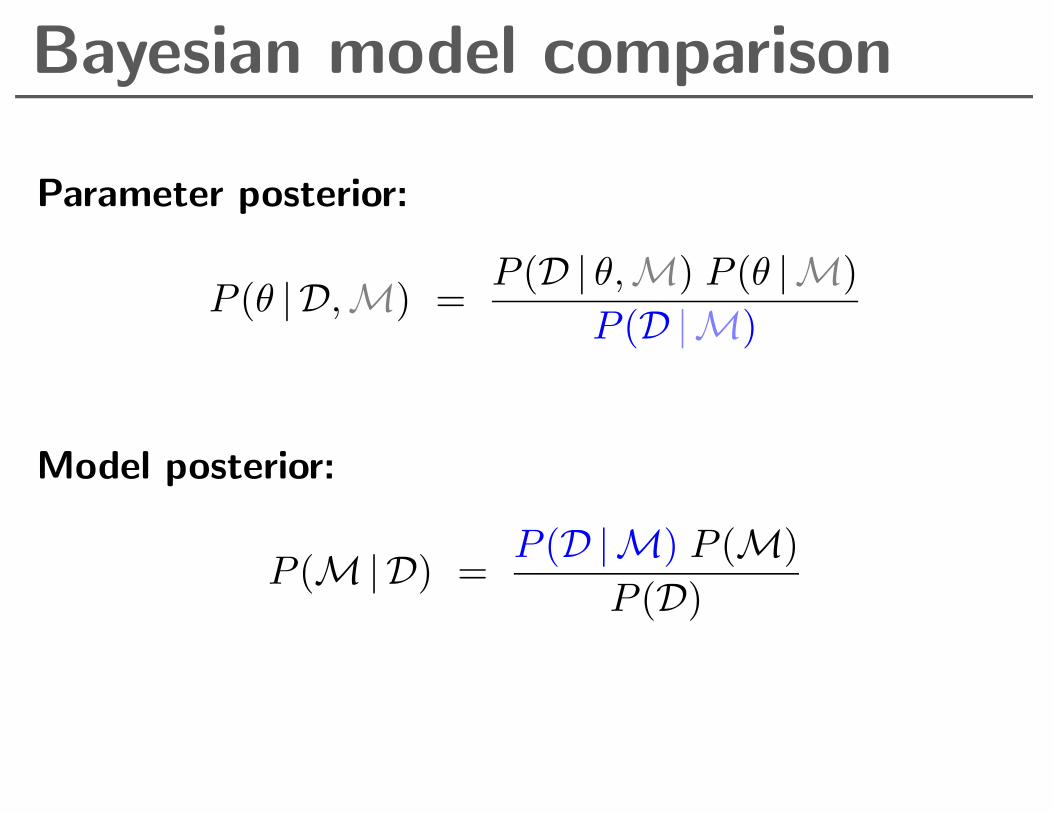
Bayesian model comparison
Parameter posterior:
P (θ | D,M) =P (D | θ,M) P (θ |M)
P (D |M)
Model posterior:
P (M|D) =P (D |M) P (M)
P (D)
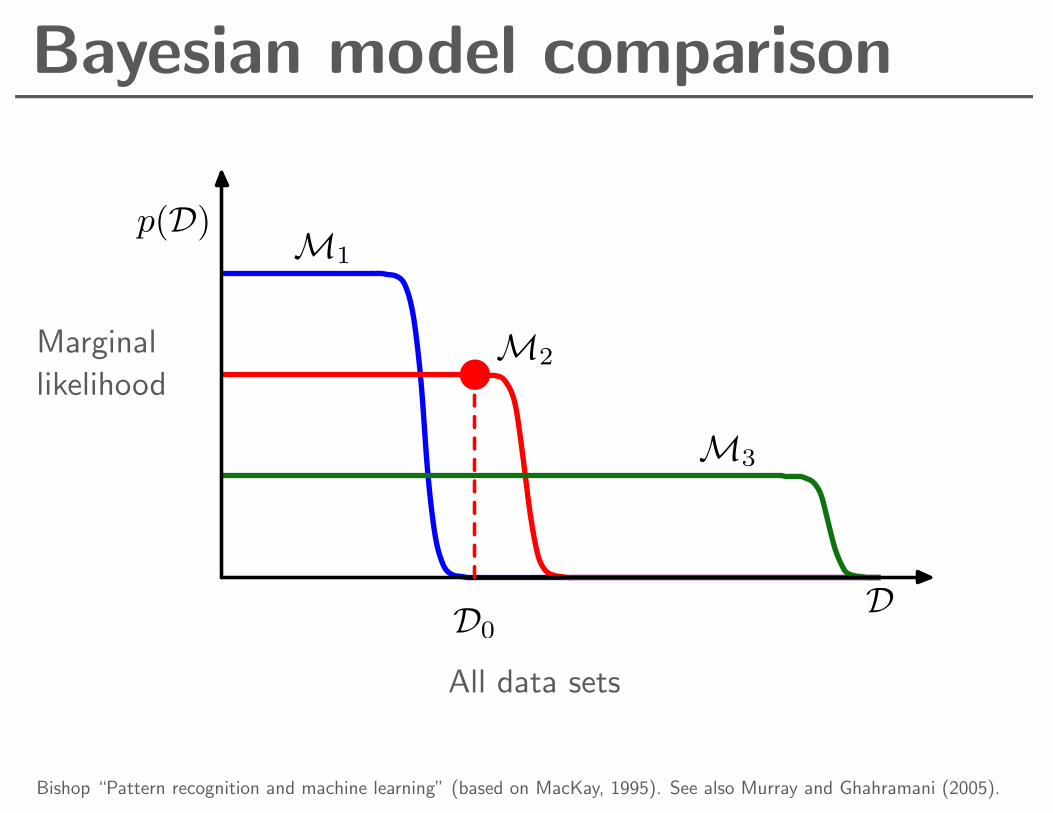
Bayesian model comparison
Marginal
likelihood
p(D)
DD0
M1
M2
M3
All data sets
Bishop “Pattern recognition and machine learning” (based on MacKay, 1995). See also Murray and Ghahramani (2005).
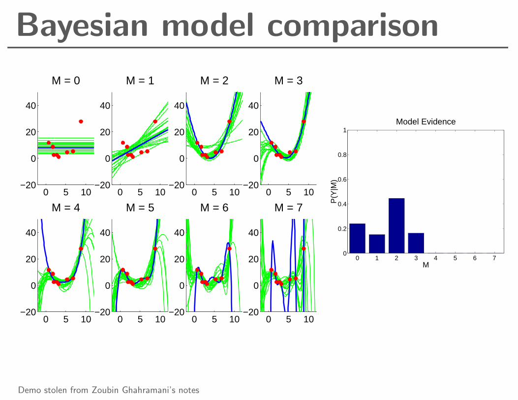
Bayesian model comparison
0 5 10−20
0
20
40
M = 0
0 5 10−20
0
20
40
M = 1
0 5 10−20
0
20
40
M = 2
0 5 10−20
0
20
40
M = 3
0 5 10−20
0
20
40
M = 4
0 5 10−20
0
20
40
M = 5
0 5 10−20
0
20
40
M = 6
0 5 10−20
0
20
40
M = 7
0 1 2 3 4 5 6 70
0.2
0.4
0.6
0.8
1
M
P(Y
|M)
Model Evidence
Demo stolen from Zoubin Ghahramani’s notes
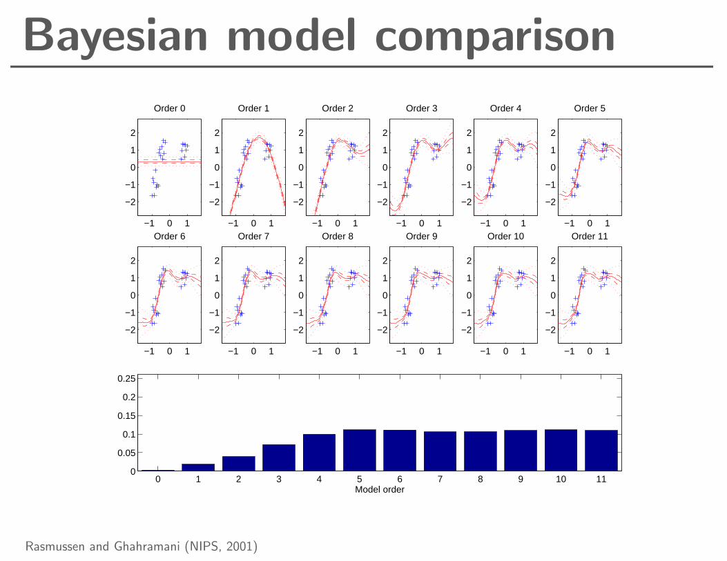
Bayesian model comparison
−1 0 1
−2
−1
0
1
2
Order 0
−1 0 1
−2
−1
0
1
2
Order 1
−1 0 1
−2
−1
0
1
2
Order 2
−1 0 1
−2
−1
0
1
2
Order 3
−1 0 1
−2
−1
0
1
2
Order 4
−1 0 1
−2
−1
0
1
2
Order 5
−1 0 1
−2
−1
0
1
2
Order 6
−1 0 1
−2
−1
0
1
2
Order 7
−1 0 1
−2
−1
0
1
2
Order 8
−1 0 1
−2
−1
0
1
2
Order 9
−1 0 1
−2
−1
0
1
2
Order 10
−1 0 1
−2
−1
0
1
2
Order 11
0 1 2 3 4 5 6 7 8 9 10 110
0.05
0.1
0.15
0.2
0.25
Model order
Rasmussen and Ghahramani (NIPS, 2001)
Bayesian linear regression (with RBF features)
−4 −2 0 2 4
−5
0
5
0
0.5
1
P (θ |Data) ∝ P (Data | θ) P (θ)
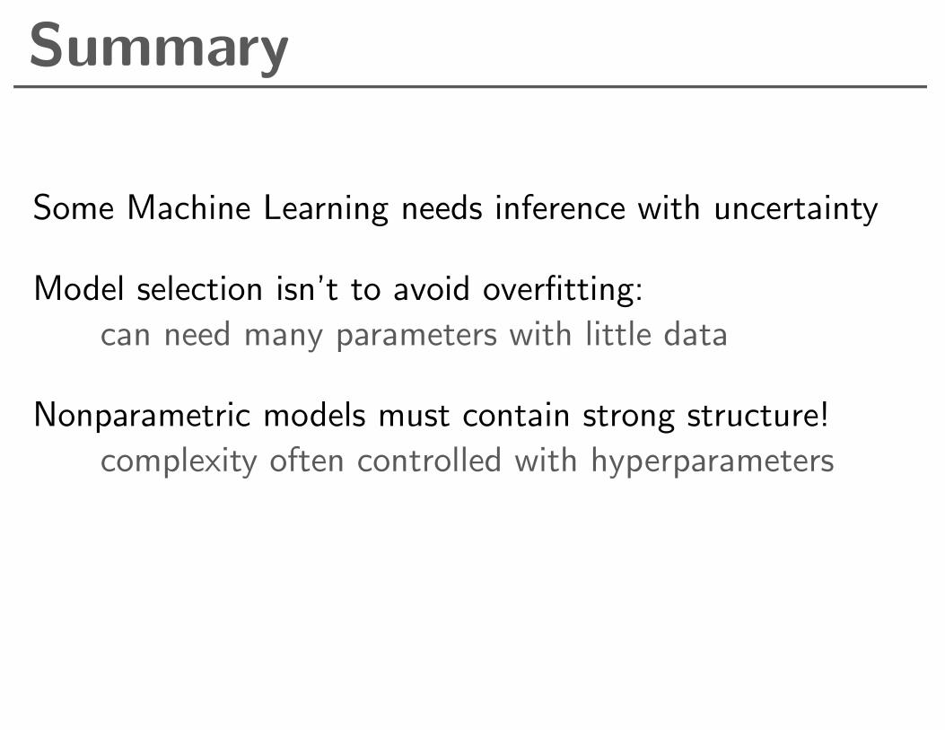
Summary
Some Machine Learning needs inference with uncertainty
Model selection isn’t to avoid overfitting:
can need many parameters with little data
Nonparametric models must contain strong structure!
complexity often controlled with hyperparameters

The messy truth
100 200 300 400 5000
0.02
0.04
0.06
0.08
0.10
Evidence
Al l data sets, D
10 20 30 40 50 60 70 80 900
0.02
0.04
0.06
0.08
0.10
Evi
den
ce
Subset of possible data sets, D
(a)
(b) (c)(d)
(e)
(f)(g)
(h)
P (D|H3)P (D|H2)P (D|H1)P (D|H0)
Murray and Ghahramani (2005).
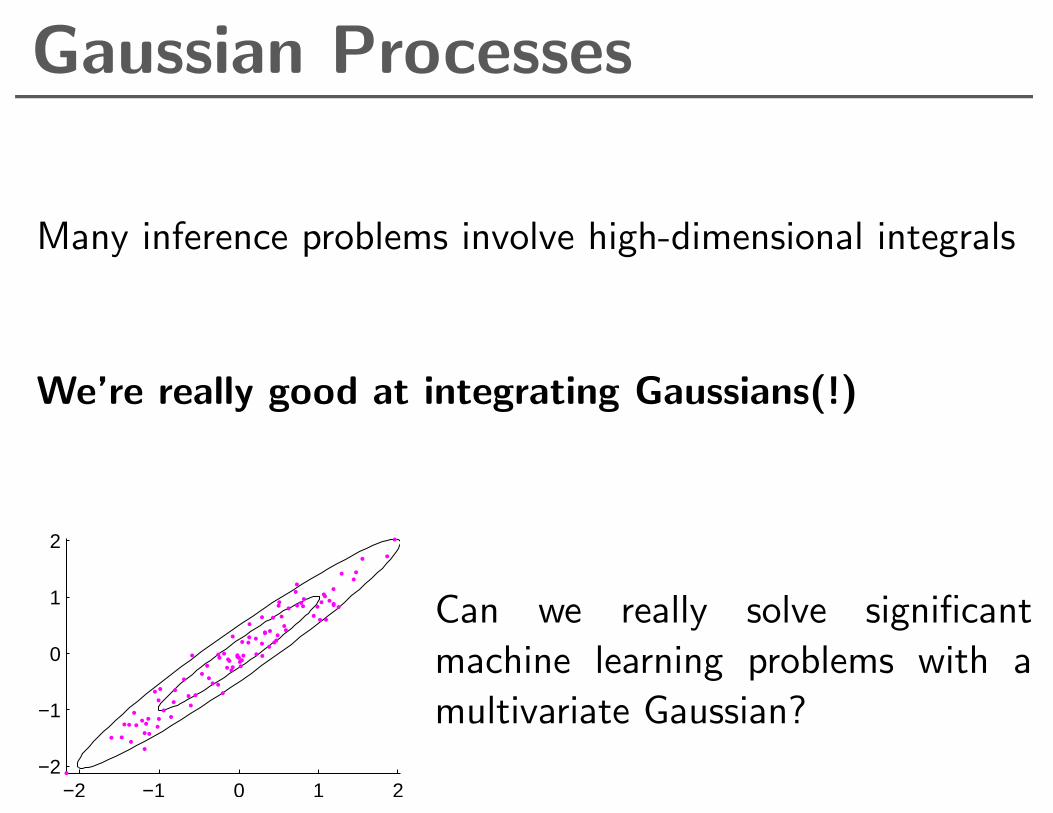
Gaussian Processes
Many inference problems involve high-dimensional integrals
We’re really good at integrating Gaussians(!)
−2 −1 0 1 2−2
−1
0
1
2
Can we really solve significant
machine learning problems with a
multivariate Gaussian?

Gaussian distributions
Completely described by mean µ and covariance Σ:
P (f |Σ, µ) = |2πΣ|−12 exp
(− 1
2(f − µ)TΣ−1(f − µ))
Where Σij = 〈fifj〉 − µiµj
If we know a distribution is Gaussian and know its mean
and covariances, we know its density function.

Marginal of Gaussian
The marginal of a Gaussian distribution is Gaussian.
P (f ,g) = N([
a
b
],
[A C
C> B
])As soon as you convince yourself that the marginal
P (f) =
∫dg P (f ,g)
is Gaussian, you already know the means and covariances:
P (f) = N (a, A).
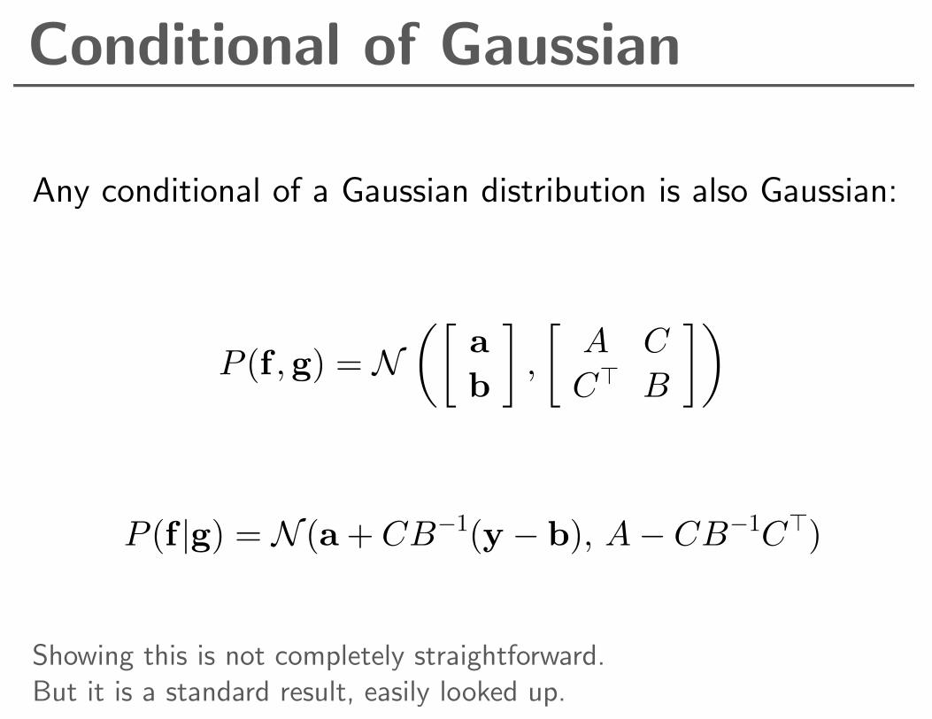
Conditional of Gaussian
Any conditional of a Gaussian distribution is also Gaussian:
P (f ,g) = N([
a
b
],
[A C
C> B
])
P (f |g) = N (a + CB−1(y − b), A− CB−1C>)
Showing this is not completely straightforward.But it is a standard result, easily looked up.
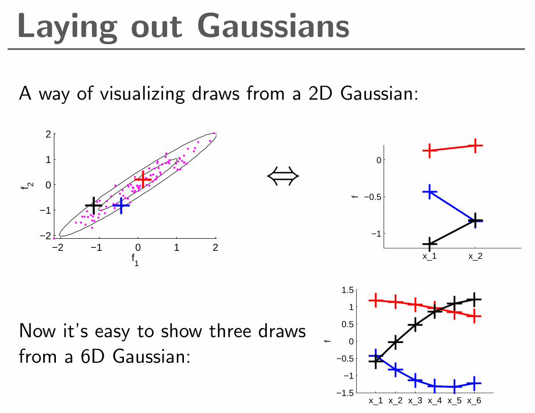
Laying out Gaussians
A way of visualizing draws from a 2D Gaussian:
−2 −1 0 1 2−2
−1
0
1
2
f1
f 2 ⇔
x_1 x_2
−1
−0.5
0
f
Now it’s easy to show three draws
from a 6D Gaussian:
x_1 x_2 x_3 x_4 x_5 x_6−1.5
−1
−0.5
0
0.5
1
1.5
f
Building large Gaussians
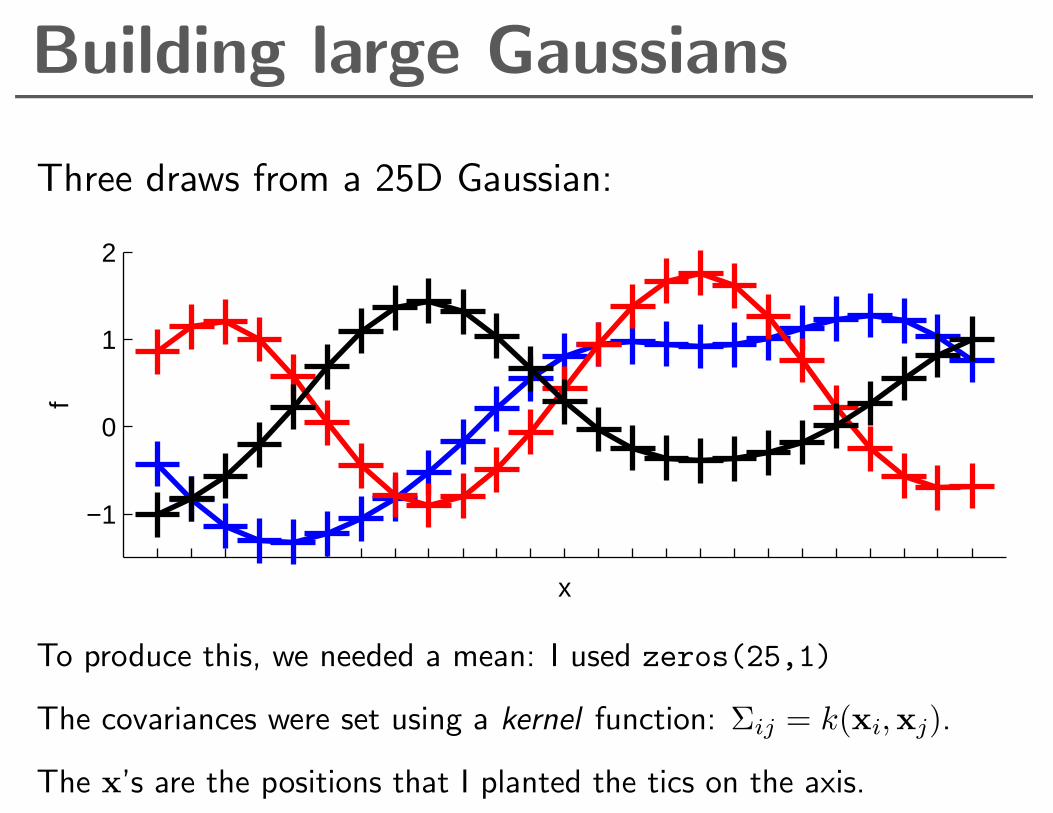
Three draws from a 25D Gaussian:
−1
0
1
2
f
x
To produce this, we needed a mean: I used zeros(25,1)
The covariances were set using a kernel function: Σij = k(xi,xj).
The x’s are the positions that I planted the tics on the axis.

GP regression model
0 0.2 0.4 0.6 0.8 1−1.5
−1
−0.5
0
0.5
1
0 0.2 0.4 0.6 0.8 1−1.5
−1
−0.5
0
0.5
1
f ∼ GP
f ∼ N (0,K), Kij = k(xi, xj)
where fi = f(xi)
Noisy observations:
yi|fi ∼ N (fi, σ2n)
GP Posterior
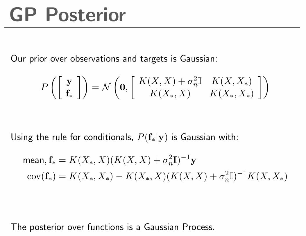
Our prior over observations and targets is Gaussian:
P
([y
f∗
])= N
(0,
[K(X,X) + σ2
nI K(X,X∗)
K(X∗, X) K(X∗, X∗)
])
Using the rule for conditionals, P (f∗|y) is Gaussian with:
mean, f∗ = K(X∗, X)(K(X,X) + σ2nI)−1y
cov(f∗) = K(X∗, X∗)−K(X∗, X)(K(X,X) + σ2nI)−1K(X,X∗)
The posterior over functions is a Gaussian Process.
GP posterior
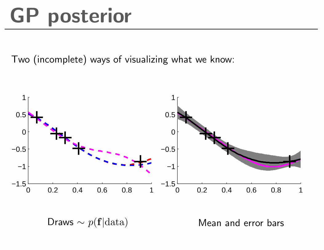
Two (incomplete) ways of visualizing what we know:
0 0.2 0.4 0.6 0.8 1−1.5
−1
−0.5
0
0.5
1
0 0.2 0.4 0.6 0.8 1−1.5
−1
−0.5
0
0.5
1
Draws ∼ p(f |data) Mean and error bars

Gaussian Process Summary
We can represent a function as a big vector f
We assume that this unknown vector was drawn from a big correlated
Gaussian distribution, a Gaussian process.
(This might upset some mathematicians, but for all practical machine learning and statistical problems, this is fine.)
Observing elements of the vector (optionally corrupted by Gaussian
noise) creates a posterior distribution. This is also Gaussian: the
posterior over functions is still a Gaussian process.
Because marginalization in Gaussians is trivial, we can easily ignore all
of the positions xi that are neither observed nor queried.

Appendix Slides
Card prediction
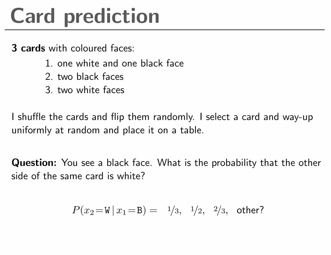
3 cards with coloured faces:
1. one white and one black face
2. two black faces
3. two white faces
I shuffle the cards and flip them randomly. I select a card and way-up
uniformly at random and place it on a table.
Question: You see a black face. What is the probability that the other
side of the same card is white?
P (x2=W |x1=B) = 1/3, 1/2, 2/3, other?

Notes on the card prediction problem:
This card problem is Ex. 8.10a), MacKay, p142.
http://www.inference.phy.cam.ac.uk/mackay/itila/
It is not the same as the famous ‘Monty Hall’ puzzle: Ex. 3.8–9 and
http://en.wikipedia.org/wiki/Monty_Hall_problem
The Monty Hall problem is also worth understanding. Although the
card problem is (hopefully) less controversial and more
straightforward. The process by which a card is selected should be
clear: P (c) = 1/3 for c = 1, 2, 3, and the face you see first is chosen at
random: e.g., P (x1=B|c=1) = 0.5.
Many people get this puzzle wrong on first viewing (it’s easy to mess
up). If you do get the answer right immediately (are you sure?), this
is will be a simple example on which to demonstrate some formalism.
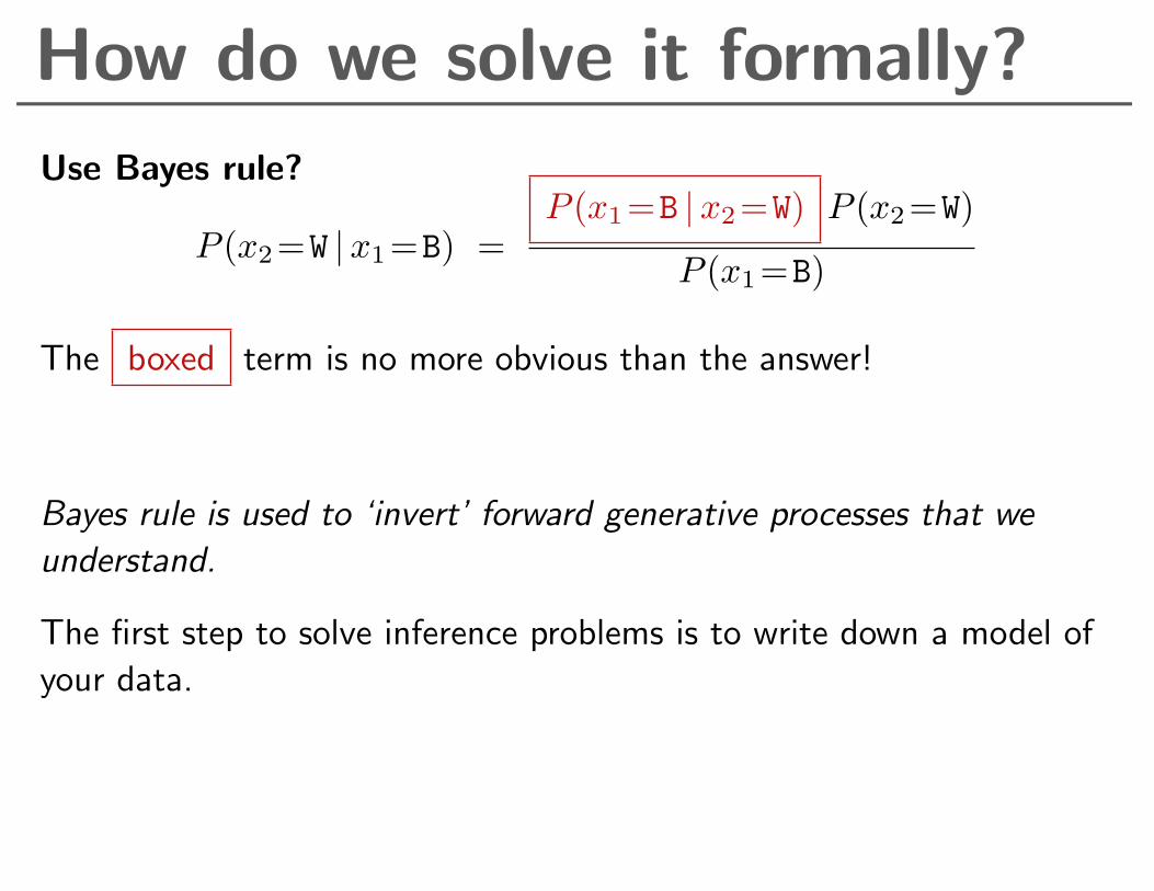
How do we solve it formally?
Use Bayes rule?
P (x2=W |x1=B) =P (x1=B |x2=W) P (x2=W)
P (x1=B)
The boxed term is no more obvious than the answer!
Bayes rule is used to ‘invert’ forward generative processes that we
understand.
The first step to solve inference problems is to write down a model of
your data.

The card game model
Cards: 1) B|W, 2) B|B, 3) W|W
P (c) =
{1/3 c = 1, 2, 3
0 otherwise.
P (x1=B | c) =
1/2 c = 1
1 c = 2
0 c = 3
Bayes rule can ‘invert’ this to tell us P (c |x1=B);
infer the generative process for the data we have.
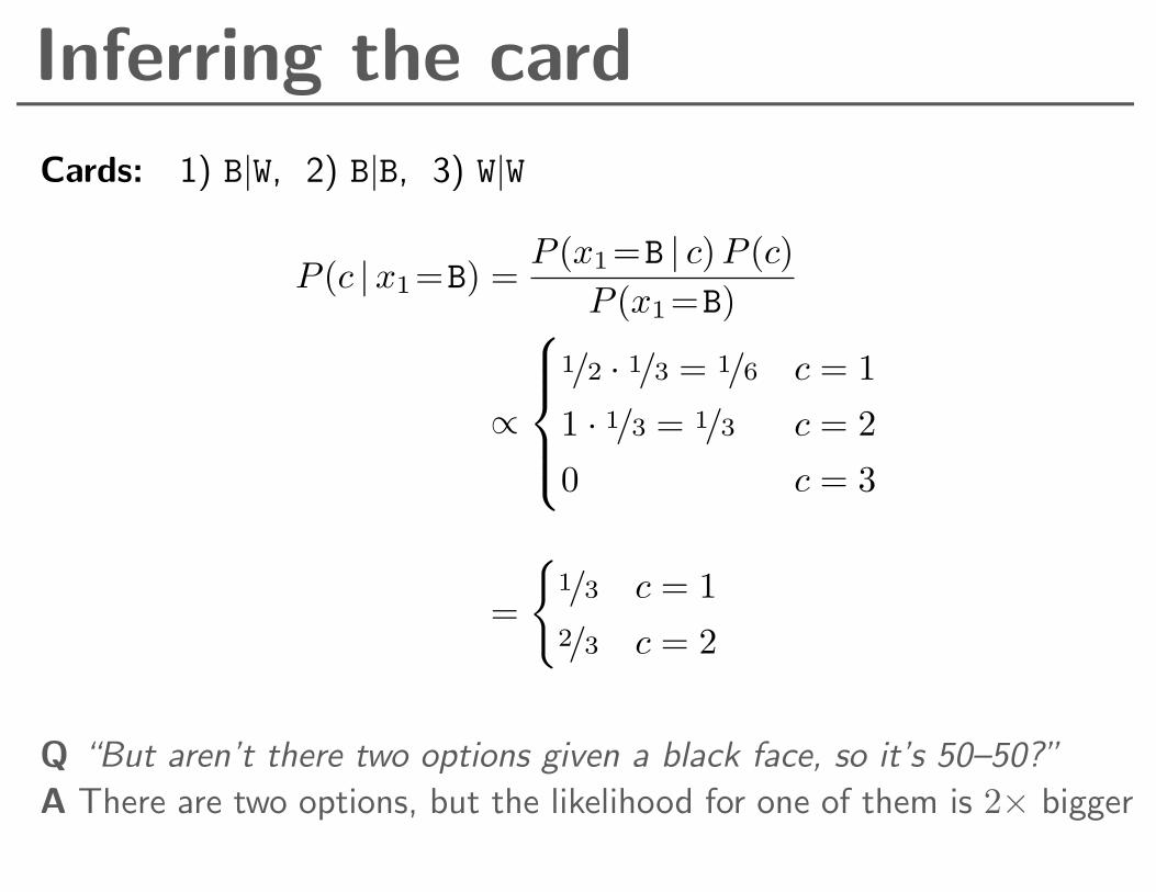
Inferring the card
Cards: 1) B|W, 2) B|B, 3) W|W
P (c |x1=B) =P (x1=B | c)P (c)
P (x1=B)
∝
1/2 · 1/3 = 1/6 c = 1
1 · 1/3 = 1/3 c = 2
0 c = 3
=
{1/3 c = 1
2/3 c = 2
Q “But aren’t there two options given a black face, so it’s 50–50?”
A There are two options, but the likelihood for one of them is 2× bigger
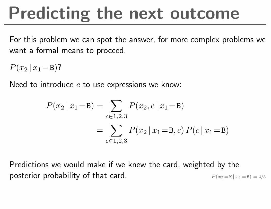
Predicting the next outcome
For this problem we can spot the answer, for more complex problems we
want a formal means to proceed.
P (x2 |x1=B)?
Need to introduce c to use expressions we know:
P (x2 |x1=B) =∑
c∈1,2,3P (x2, c |x1=B)
=∑
c∈1,2,3P (x2 |x1=B, c)P (c |x1=B)
Predictions we would make if we knew the card, weighted by the
posterior probability of that card. P (x2=W | x1=B) = 1/3
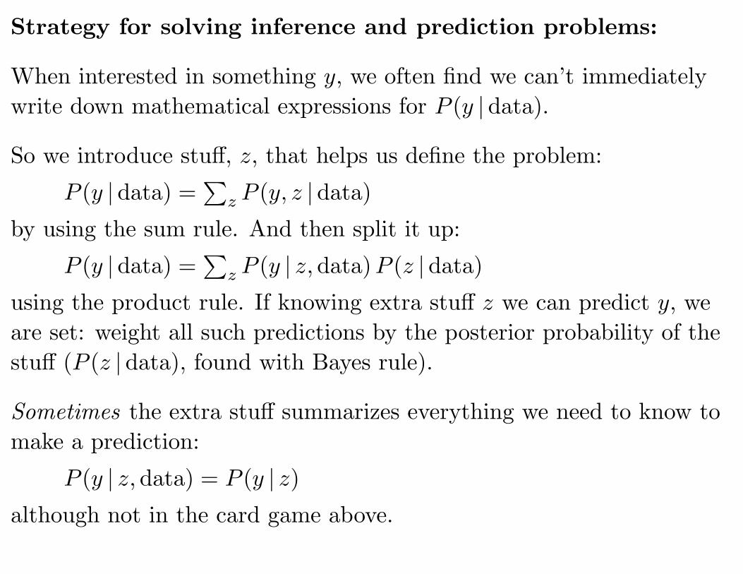
Strategy for solving inference and prediction problems:
When interested in something y, we often find we can’t immediately
write down mathematical expressions for P (y |data).
So we introduce stuff, z, that helps us define the problem:
P (y |data) =∑
z P (y, z |data)
by using the sum rule. And then split it up:
P (y |data) =∑
z P (y | z,data)P (z |data)
using the product rule. If knowing extra stuff z we can predict y, we
are set: weight all such predictions by the posterior probability of the
stuff (P (z |data), found with Bayes rule).
Sometimes the extra stuff summarizes everything we need to know to
make a prediction:
P (y | z,data) = P (y | z)although not in the card game above.
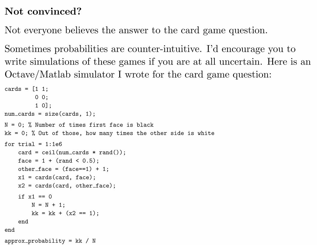
Not convinced?
Not everyone believes the answer to the card game question.
Sometimes probabilities are counter-intuitive. I’d encourage you to
write simulations of these games if you are at all uncertain. Here is an
Octave/Matlab simulator I wrote for the card game question:
cards = [1 1;
0 0;
1 0];
num cards = size(cards, 1);
N = 0; % Number of times first face is black
kk = 0; % Out of those, how many times the other side is white
for trial = 1:1e6
card = ceil(num cards * rand());
face = 1 + (rand < 0.5);
other face = (face==1) + 1;
x1 = cards(card, face);
x2 = cards(card, other face);
if x1 == 0
N = N + 1;
kk = kk + (x2 == 1);
end
end
approx probability = kk / N