D3.2 Data fusion - Traffic Project: ROADIDEA 215455 Document Number and Title: D3.2 Data fusion - Traffic Work-Package: WP3.2 Deliverable Type: Report Contractual Date of Delivery: 30.11.2008 Actual Date of Delivery: 30.11.2008 Author/Responsible(s): Olle Wedin (Semcon) Contributors: Igor Grabec (Amanova)

Ville Könönen (VTT) Matthieu Molinier (VTT) Sami Nousiainen (VTT) Esben Almquist (Klimator)

Approval of this report: Coordinator, Technical Committee Summary of this report: Report presents several methods for modeling traffic.

Filtered data is used as input to algorithms that are developed to model and predict traffic characteristics during normal weather conditions.

Keyword List: Data fusion, traffic models, traffic information, weather information, road conditions

Dissemination level: Public (PU)

ROADIDEA 215455

Change History Version Date Status Author (Partner) Description

0.1 22/10 2008 Draft Olle Wedin (Semcon) 1st draft 0.2 12/11 2008 Draft Olle Wedin (Semcon)

Igor Grabec (AMANOVA) Ville Könönen (VTT)

2nd draft

0.3 25/11 2008 Draft Olle Wedin (Semcon) Igor Grabec (AMANOVA) Ville Könönen (VTT)

Final draft

0.4 26/11 2008 Draft P. Saarikivi (FORC) Editorial check 1.0 30/11 2008 Final TCC Final check 1.1 26/05 2009 Final P. Saarikivi (FORC) Front page with flag

Distribution list European Commission Emilio Davila Gonzalez

Wolfgang Höfs

ROADIDEA partners E-mail list www.roadidea.eu

ROADIDEA 215455

Abstract Many methods for modelling traffic exist. The majority of them use the same set of basic building blocks. These are explained, as well as some of the methods. A list of earlier works in the field of traffic modelling is provided. One method (general regression) is selected to exemplify the use, and result on real data. This is described in detail and used to predict traffic flow. Also one method of modelling traffic flow via a sum of normal distributions is described briefly. A method for evaluating the performance of the models is also provided and exemplified.

Table of contents 1 Introduction........................................................................................................1

1.1 Background ................................................................................................1 1.2 Objectives ..................................................................................................2 1.3 Method.......................................................................................................2

2 Fundamentals of traffic modeling.........................................................................2 2.1 Measurements and data..............................................................................2

2.1.1 Measurement types .............................................................................2 2.1.2 Distance measures ..............................................................................3 2.1.3 Data quality.........................................................................................4

2.2 Modeling ....................................................................................................4 2.2.1 Predictive modeling .............................................................................5 2.2.2 Descriptive modeling ...........................................................................6 2.2.3 Bibliography ........................................................................................9

2.3 Relevant methods for the traffic domain......................................................10 2.3.1 Travel time prediction and travel data mining .......................................13 2.3.2 Friction and road surface condition .....................................................14 2.3.3 Traffic accidents ................................................................................15 2.3.4 Utilization of weather information ........................................................15

3 Specific traffic model ........................................................................................17 3.1 General regression ...................................................................................18

4 Examples with results from traffic flow modeling.................................................20 4.1 An example of traffic flow modeling and forecasting ....................................21 4.2 Estimation of modeling and forecasting accuracy ........................................22 4.3 Modeling of traffic flow field .......................................................................25 4.4 Completion and correction of data by a model ............................................26 4.5 Modeling of traffic flow by normal distributions ............................................29

5 Joining of weather and traffic data .....................................................................32 5.1 Classification of road weather ....................................................................32 5.2 Inclusion of weather variables into traffic flow modeling ...............................32

6 A route to intelligent traffic control .....................................................................36 7 Summary and conclusions ................................................................................38 8 References ......................................................................................................38

ROADIDEA 215455

1

1 Introduction The main objective of work package 3 “WP3 - Method and model development” is converting data into information; to use data from work package two as input and by models/data fusion produce valuable and correct information as an output. In order to achieve this, methods for filtering input data from errors have to be developed and implemented, as well as models to extract information from the filtered data. Methods to quantify and estimate their performance also play an important role. This document is a report of sub-package 2 of WP3 “WP3.2 Data fusion -Traffic ”. It will, as its name implies, deal with the second link in the chain above: data fusing. Data fusion refers to the group of data analysis that involves treatment of data of many kinds, from many sources. The aim of this sub work package is to use the filtered data from WP3.1 as input to algorithms that are developed to model and predict traffic characteristics, during normal weather conditions. Coming sub packages of WP3 (WP3.3 and WP3.4) will use the outcome of this report and add weather as an explicit input to estimate changes in states caused by weather, such road surface conditions. Much effort has been put into this topic already and references to previous work are given in section 2.

1.1 Background Road traffic is a consequence of population activity to which many agents (~100 M) participate.[1,2] In spite of this, the traffic flow does not exhibit completely random character because the population activity is synchronized to a high degree. The synchronization is stimulated externally by changing properties of the environment, as well as internally by social agreements about working days and holidays. The external stimulation can be physically described by the time and weather variables, while the internal one has to be modeled by some specific dynamic law. In agreement with these properties we treat road traffic as an example of very complex deterministic chaos.[3] Due to external influences we further treat the road traffic flow as a stochastic non-autonomous dynamic phenomenon and try to model its generating equation statistically. The basic information for the creation of the model can be extracted from records of traffic flow rate and related environmental variables. For this purpose a general non-parametric statistical method is proposed in section 1.3, while in the subsequent ones the applicability of the method is demonstrated by examples of traffic flow prediction in various countries. The performance of the proposed method is quantitatively estimated by a cross-validation method (section 3.5 of deliverable 3.1). It is based on estimation of the correlation coefficient between predicted and actually measured traffic data. Examination of the correlation coefficient dependence on the structure of the condition indicates how the method can be tuned to a specific case of modeling.

ROADIDEA 215455

2

1.2 Objectives • Provide an introduction to basic concepts involved in traffic modeling. • Find and present references to previous work and knowledge involved in traffic

modeling. • Present one approach of quantitative forecasting of traffic flow rate, which can

work as an efficient information support to participants in road traffic. • Give examples where the approach above is used on real data.

1.3 Method In accordance with the problem specified above, our goal is to extract from experimental data relations that describe dynamic properties of the transport system. For this purpose we apply general methods of statistical estimators that lead us to the modeling of traffic phenomenon in terms experimental data.[3] In the section 0 and forwards, this approach is tested. We limit our consideration to the traffic on roads and avoid description of the evolution of roads infrastructure. Before the specific method is described, the fundamentals of road traffic modeling will be presented.

2 Fundamentals of traffic modeling This section serves as a stepping-stone for the remaining sections of the document. We try to provide a brief outline of available data analysis methods and applicability of them to traffic related problem domains. We start the section by focusing on data, different types of the data and the quality issues. Then we proceed with discussing how to use data to model a physical phenomena and how to visualize multi-dimensional data sets.

2.1 Measurements and data Data are collected by observing entities in the environment of interest and setting values of the variables according to the properties of these entities. The relationships between different entities can be represented by using relationships between different variables. These relationships depend heavily on the measurement types and the concept of distance between entities. The results of the data analysis depend heavily on the quality of the data; both quality of individual samples and the whole data set.

2.1.1 Measurement types Measurement type is a classification of the variable reflecting nature of information that the variable contains. The measurement type information stipulates which mathematical operations can be applied to the variables. Hence, the term level of measurement is also used in this context illustrating the fact that it is possible to construct a hierarchical structure based on the measurement types according to the number of available mathematical operators for the variables.

ROADIDEA 215455

3

The lowest level of measurement is the nominal measurement level. A nominal variable assigns only a name for a property. For example, if we have a variable corresponding to the color of a car, the variable can get values likes red, black, etc. The only mathematical operation available for nominal variables is the equality operation (=). For example it is possible to deduct whether two cars share the same color. The second lowest level of measurement is the ordinal measurement level. The ordinal variable is used to rank entities in the environment of interest. For example, in a voting procedure, the options are put to an order. In addition to equality operation, comparisons (<, >) are available for ordinal measurements. The second highest measurement level is the interval measurement level. In addition to the comparison operations, also differences between objects can be defined. Therefore averaging and subtraction are allowed for interval variables. The highest measurement level is the ratio level. On this level, also a ratio between two measurements is defined. Operations such as multiplication and addition are allowed. Most physical measurements, e.g. mass or temperature belong to this level of measurements.

2.1.2 Distance measures Many data analysis and modeling methods rely on the concept of similarity (or more generally, proximity) between entities in environment of interest. Usually similarity of two entities is calculated from a vector form representation collecting values of several measurements. An element in the vector is of one of the measurement types discussed in the previous subsection. When handling similarity of entities formally, a mathematical concept of dissimilarity measure is used. Dissimilarity measure can be arbitrary but usually it is required that the measure fulfills the conditions of metric. A dissimilarity measure ),( yxd is metric if it fulfills the following conditions ( zyx ,, ) are arbitrary entities in the environment):

1. yxyxd ,0),( ∀≥ and 0),( =yxd iff yx = . 2. yxxydyxd ,),(),( ∀= 3. zyxyzdzxdyxd ,,),(),(),( ∀+≤

The condition 3 is called the triangle inequality. Sometimes this condition is relaxed and the corresponding dissimilarity measure is called pseudometric. Example metrics are for example Euclidean distance or more general dissimilarity measure called Minkowski distance. If we denote an element i of an entity j as

jix , Minkowski metric is as follows:

ROADIDEA 215455

4

λλ1

1))((),( ∑

=

−=N

i

yi

xi xxyxd ,

where N is the dimensionality of the vector containing measurements of the entities and λ is a positive integer. By setting 1=λ we get a Manhattan distance and 2=λ leads to the Euclidean distance.

2.1.3 Data quality The data quality has a crucial role in the usefulness of the results of the data analysis. Data quality can be divided into two main categories: data quality of the individual samples and the quality of the whole dataset. Let us start by considering the measurement process itself in which we measure different properties of the object of interest. Perhaps the most important quality metric related to the measurements is precision. If we measure the same object several times in a constant environment, the variance of the measurements is small if the precision of the measument process is high. In addition, if the measurement process is also accurate, it yields to the measurements that are very close to the true value of the property. Third important property directly related to the measurement process is the validity of the measurements. The measurements are valid only if they measure the property that they are supposed to measure. In addition to the quality of the individual measurement, the quality of the whole dataset affects a lot of the quality of the analysis results. The most important property of a dataset is that it should contain samples that represent the domain of interest as well as possible. For example, if we are measuring body mass indeces (BMI) of the whole population in some country, say Finland, the sample should be carefully chosen as for example educational background and occupation have a significant effect on the average BMI. Often measurement process also produces anomalous observations or outliers that should be filtered out before data analysis phase. In one dimensional case, these outliers can be easily detected visually. In multi-dimensional case, outlier detection is much harder and requires deep understanding of the underlying phenomena.

2.2 Modeling A model is a high level description of the data summarizing high-level characteristics of the data set. The model can be either descriptive or predictive. Descriptive models provide a summary or a human interpretable view of complex dataset and hence allows us to make decisions based on the data. Predictive models try to predict a value of the process form which the data is collected, for example estimate of the future value of a share. We start the section by introducing two predictive modeling tools, namely regression and classification. Then we proceed with different descriptive modeling

ROADIDEA 215455

5

techniques. Finally we present a short bibliography containing literature pointers to the relevant books on the domain.

2.2.1 Predictive modeling The goal of the regression as a predictive modeling method is to generalize, i.e. predict the behavior of a system based on the previous observations. The variables that are used as inputs for the prediction system are called predictor variables and the variable to be predicted is the response variable. In regression, the response variable normally gets numerical values. A classification task can be seen as building a model which maps a measurement vector

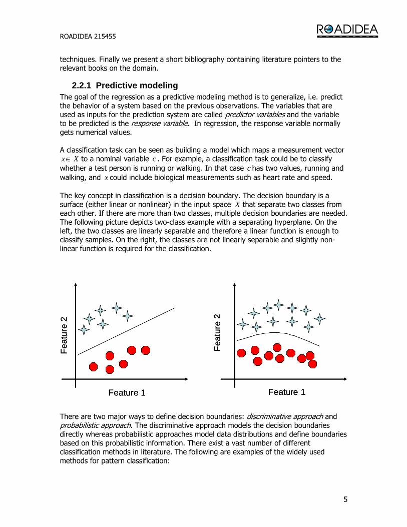
Xx ∈ to a nominal variable c . For example, a classification task could be to classify whether a test person is running or walking. In that case c has two values, running and walking, and x could include biological measurements such as heart rate and speed. The key concept in classification is a decision boundary. The decision boundary is a surface (either linear or nonlinear) in the input space X that separate two classes from each other. If there are more than two classes, multiple decision boundaries are needed. The following picture depicts two-class example with a separating hyperplane. On the left, the two classes are linearly separable and therefore a linear function is enough to classify samples. On the right, the classes are not linearly separable and slightly non-linear function is required for the classification. There are two major ways to define decision boundaries: discriminative approach and probabilistic approach. The discriminative approach models the decision boundaries directly whereas probabilistic approaches model data distributions and define boundaries based on this probabilistic information. There exist a vast number of different classification methods in literature. The following are examples of the widely used methods for pattern classification:

Feature 1

Feat

ure

2

Feature 1

Feat

ure

2

Feature 1

Feat

ure

2

Feature 1

Feat

ure

2

ROADIDEA 215455

6

• k-Nearest Neighbor classifier (kNN). Each sample is classified to the class that occurs most often in its neighborhood (with respect to some metric, e.g. Euclidean distance).

• Minimum-distance classifier. Each sample is compared to the class mean vectors and the nearest class is then selected.

• Bayesian classifiers. A priori probability distributions of the data are converted to posteriori distributions by using Bayes rule. Depending on the distributions and underlying assumptions this leads to several actual classification methods.

Note the major difference between regression techniques and classification techniques is that in the regression models the output of the system is numeric but in classification it is usually nominal.

2.2.2 Descriptive modeling Descriptive modeling methods are also known as exploratory analysis or unsupervised classification, because there is no a-priori knowledge available about the class labels to create the data model. Descriptive models are meant to be a summary of a usually large dataset. For example, the mean or variance of a single variable, or its histogram, are simple descriptive models of that variable, i.e. quantities that describe in a compact way the data content. The correlation coefficients between two variables of a dataset can also be seen as a descriptive model of the relationship between those two variables – the higher the correlation coefficient, the mode the variables are inter-related. Dimensionality reduction techniques such as Principal Component Analysis are also sometimes viewed as descriptive modeling, in the sense that they provide a more compact description of a dataset and explain how the data is organized. There exist a large amount of more or less complex descriptive models, that can be grouped into two main categories : Clustering : the dataset is partitioned into groups Density estimation : the probability distribution is estimated from data points

2.2.2.1 Clustering Clustering is also called unsupervised classification. A cluster is a group of data points that share similar properties. Each data point is described by a pattern or feature vector, which define the dimension of the feature space. The key principle to clustering is similarity between pattern vectors according to a distance or similarity measure in the feature space : pattern vectors close to each other form a same cluster, whereas dissimilar vectors belong to other clusters. Ideally the clusters should be homogeneous (minimal deviation within clusters) and well differentiated groups (maximal distance between clusters). Each cluster is represented by a unique feature vector, generally derived by averaging the feature vectors of the cluster points.

There are numerous types of clustering methods :

ROADIDEA 215455

7

In sequential clustering, a unique clustering is produced. The data points are presented a few times to the clustering method, and the result is dependent from the order in which the points were fed into the algorithm.

In Hierarchical clustering, the tree structure defines how pattern vectors are attached to clusters. Clusters at the fine level of the hierarchy are embedded in clusters at the coarser level. This is especially suited to describe categories and sub-categories in the data, as for example in biology for clustering species. Hierarchical clustering algorithms are usually iterative and can be either : agglomerative if starting from a high number of clusters and reducing at the next level. Clusters are merged through matrix or graph theory. Agglomerative algorithms are suited to create elongated clusters (single link algorithm) or compact clusters (complete link algorithm). divisive when the number of clusters increases at each step. A large number of clustering algorithms are based on the optimization of a cost function. Usually the number of clusters has to be chosen beforehand. Hard clustering is when a pattern vector can belong to one and only one cluster. Most well-known algorithms are k-means or ISODATA algorithm. Clusters are defined by their means or centroïd, and constitute a partition of the ensemble of data points. Probabilistic clustering is a variant of hard clustering, where a point is assigned to the cluster that has the highest a posteriori probability of containing that point. In fuzzy clustering, the membership of a point to a cluster can be quantified by a probability function. There are other clustering algorithms of various nature : genetic clustering algorithms are iterative and inspired from principles of population evolution (through merging and random selection) boundary detection methods focuses on the separation between clusters rather than clusters themselves competitive learning algorithms are iterative schemes without cost function. Self-Organising Map algorithm is based on competitive learning. The Self-Organising Map (SOM) is a neurally motivated unsupervised learning technique, forming a nonlinear mapping of a high-dimensional input space to a typically two-dimensional grid of neural units. During SOM training, the model vectors in its neurons get values which form a topology-preserving mapping : neighboring vectors in the input space are mapped into nearby units on the SOM grid. Patterns mutually similar in respect to a feature are closely located on the SOM surface. The Self-Organising Map is known to perform well for finding clusters in high dimensional input spaces.

ROADIDEA 215455

8

2.2.2.2 Density estimation

Density estimation is the construction of an estimate, based on observed data, of an underlying probability density function that is not directly observable. There are parametric models such as single multivariate Gaussian estimate, semi-parametric mixture models (mixture of Gaussians), or non-parametric models like histogram, Parzen windows and k-Nearest Neighbor density estimation.

The histogram method is the simplest way to estimate density functions. The axis of the feature space is divided into n parts, forming regions (bins) in the feature space. The approximation of the probability density function (pdf) at a bin is :

Nk

Vxp N1)(ˆ =

where V is the volume of a bin (constant), kN the number of data points inside the bin and N the total number of data samples. In the multidimensional case, the d-dimension space is divided into hypercubes of side h and volume V = hd. The approximation of the pdf at a certain bin is equivalent to :

⎟⎟⎠

⎞⎜⎜⎝

⎛⎟⎠⎞

⎜⎝⎛ −

= ∑=

N

i

i

hxx

NVxp

1

11)(ˆ φ

and ( )⎩⎨⎧ ≤

=otherwise

xforx iji 0

2/11φ

Indeed, the function φ is equal to 1 for all points inside the unit hypercube centered at the origin and equal to 0 outside the hypercube. Considering a hypercube of side h centered at x, where the pdf is to be estimated, the summation of φ functions is the number of points kN falling into that hypercube. The pdf estimate is then in the same form as for the 1-dimensional histogram case. Histograms are easy to compute in low dimension spaces (typically one dimension).

Parzen Windows. The previous equation is the estimate of a continuous function (the pdf) from a summation of discrete function (the step functions φ). The idea of Parzen Windows method is then to generalize this formula using smooth functions instead of step functions. Typical examples are exponential functions, Gaussian functions, or other monotonically decreasing positive functions - the Parzen windows, also called kernels.

Rather than grouping observations together in bins like in the histogram approach, the kernel density estimator can be thought as placing small "bumps" (kernel functions) at each observation point. The estimator consists of a sum of kernels and is smoother as a result. For a fixed number of samples N, the smaller the side h of the kernel, the higher the variance. For a fixed side h, the variance decreases when the number of sampled points

ROADIDEA 215455

9

N tends to +∞. Under certain conditions easy to achieve, the Parzen windows estimate is unbiased and asymptotically consistent, which are desired properties for estimators. If there is little data, it is better to use a wide kernel, and vice-versa. Usually a large number of samples N is required, which grows exponentially with the dimension d of the feature space (curse of dimensionality).

k-Nearest Neighbors (kNN) density estimation. In the Parzen Windows case, the volume considered around each point was fixed and the number of points kN inside this volume varied. The kNN method uses the contrary, a fixed number of points kN = k, and the volume around the point x will be adapted to include k points exactly. The volume is large in low density areas and small in high density areas. The pdf estimate is given by :

)()(ˆ

xNVkxp =

This is also an unbiased and asymptotically consistent estimate of the true pdf under certain conditions.

2.2.2.3 Connection to predictive models Prediction based on clusters can be performed, i.e. by assigning a new data point to the cluster it is the closest from given a similarity measure. Both the Parzen Windows and the kNN density estimation methods can as well be applied to classification, using likelihood ratios.

2.2.3 Bibliography Markus Törmä, Remote Sensing and Data Classification course, Helsinki University of Technology, 2004. Sergios Theodoridis, Konstantinos Koutroumbas, Pattern recognition – 2nd edition, Eslevier Academic Press, 2003. Teuvo Kohonen, Self-Organizing Maps, Volume 30 of Springer Series in Information Sciences. Springer-Verlag, 3rd edition, 2001. David Hand, Heikki Mannila, Padhraic Smyth, Principles of Data Mining, The MIT Press, 2001.

ROADIDEA 215455

10

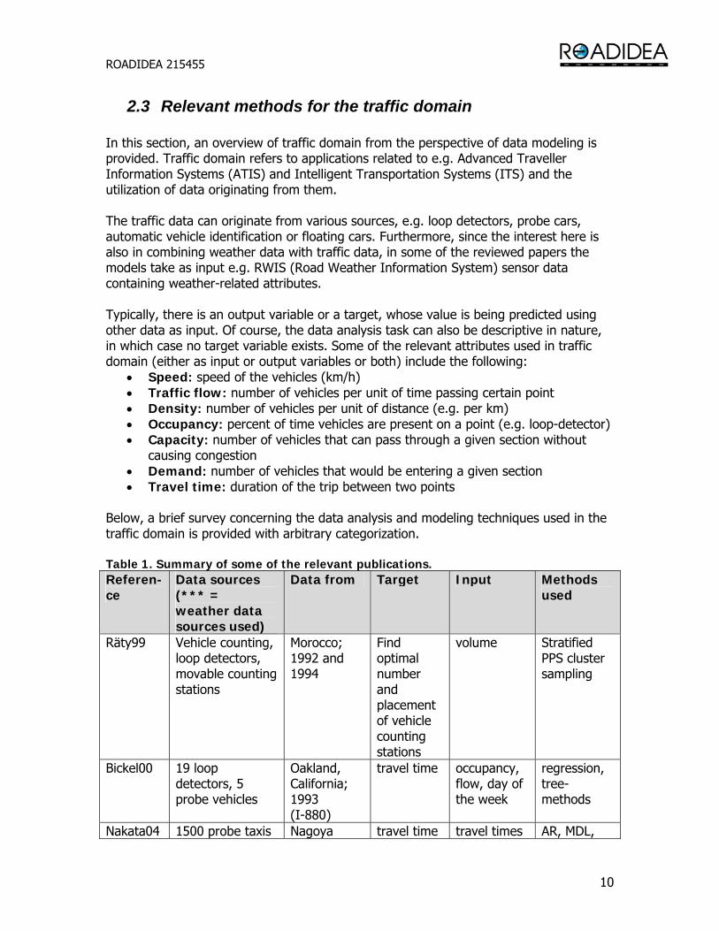
2.3 Relevant methods for the traffic domain In this section, an overview of traffic domain from the perspective of data modeling is provided. Traffic domain refers to applications related to e.g. Advanced Traveller Information Systems (ATIS) and Intelligent Transportation Systems (ITS) and the utilization of data originating from them. The traffic data can originate from various sources, e.g. loop detectors, probe cars, automatic vehicle identification or floating cars. Furthermore, since the interest here is also in combining weather data with traffic data, in some of the reviewed papers the models take as input e.g. RWIS (Road Weather Information System) sensor data containing weather-related attributes. Typically, there is an output variable or a target, whose value is being predicted using other data as input. Of course, the data analysis task can also be descriptive in nature, in which case no target variable exists. Some of the relevant attributes used in traffic domain (either as input or output variables or both) include the following:

• Speed: speed of the vehicles (km/h) • Traffic flow: number of vehicles per unit of time passing certain point • Density: number of vehicles per unit of distance (e.g. per km) • Occupancy: percent of time vehicles are present on a point (e.g. loop-detector) • Capacity: number of vehicles that can pass through a given section without

causing congestion • Demand: number of vehicles that would be entering a given section • Travel time: duration of the trip between two points

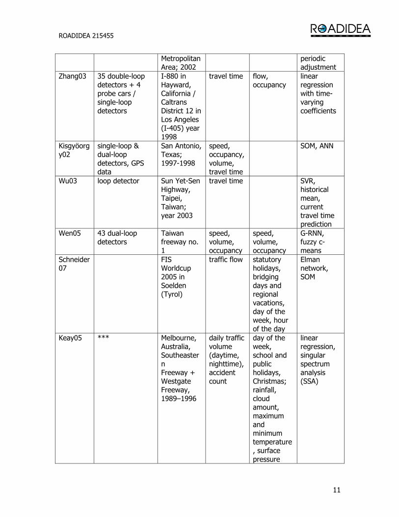
Below, a brief survey concerning the data analysis and modeling techniques used in the traffic domain is provided with arbitrary categorization. Table 1. Summary of some of the relevant publications. Referen-ce

Data sources (*** = weather data sources used)

Data from Target Input Methods used

Räty99 Vehicle counting, loop detectors, movable counting stations

Morocco; 1992 and 1994

Find optimal number and placement of vehicle counting stations

volume Stratified PPS cluster sampling

Bickel00 19 loop detectors, 5 probe vehicles

Oakland, California; 1993 (I-880)

travel time occupancy, flow, day of the week

regression, tree-methods

Nakata04 1500 probe taxis Nagoya travel time travel times AR, MDL,

ROADIDEA 215455

11

Metropolitan Area; 2002

periodic adjustment

Zhang03 35 double-loop detectors + 4 probe cars / single-loop detectors

I-880 in Hayward, California / Caltrans District 12 in Los Angeles (I-405) year 1998

travel time flow, occupancy

linear regression with time-varying coefficients

Kisgyöorgy02

single-loop & dual-loop detectors, GPS data

San Antonio, Texas; 1997-1998

speed, occupancy, volume, travel time

SOM, ANN

Wu03 loop detector Sun Yet-Sen Highway, Taipei, Taiwan; year 2003

travel time SVR, historical mean, current travel time prediction

Wen05 43 dual-loop detectors

Taiwan freeway no. 1

speed, volume, occupancy

speed, volume, occupancy

G-RNN, fuzzy c-means

Schneider07

FIS Worldcup 2005 in Soelden (Tyrol)

traffic flow statutory holidays, bridging days and regional vacations, day of the week, hour of the day

Elman network, SOM

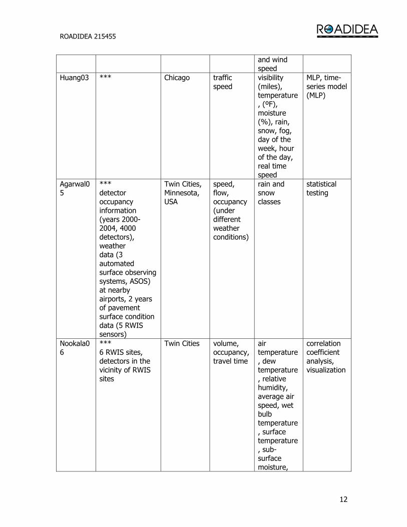
Keay05 *** Melbourne, Australia, Southeastern Freeway + Westgate Freeway, 1989–1996

daily traffic volume (daytime, nighttime), accident count

day of the week, school and public holidays, Christmas; rainfall, cloud amount, maximum and minimum temperature, surface pressure

linear regression, singular spectrum analysis (SSA)

ROADIDEA 215455

12

and wind speed

Huang03 *** Chicago traffic speed

visibility (miles), temperature, (ºF), moisture (%), rain, snow, fog, day of the week, hour of the day, real time speed

MLP, time-series model (MLP)

Agarwal05

*** detector occupancy information (years 2000-2004, 4000 detectors), weather data (3 automated surface observing systems, ASOS) at nearby airports, 2 years of pavement surface condition data (5 RWIS sensors)

Twin Cities, Minnesota, USA

speed, flow, occupancy (under different weather conditions)

rain and snow classes

statistical testing

Nookala06

*** 6 RWIS sites, detectors in the vicinity of RWIS sites

Twin Cities volume, occupancy, travel time

air temperature, dew temperature, relative humidity, average air speed, wet bulb temperature, surface temperature, sub-surface moisture,

correlation coefficient analysis, visualization

ROADIDEA 215455

13

pavement conditions

2.3.1 Travel time prediction and travel data mining Papers in this category attempt to model and predict the values of the traffic-related variables such as travel time and traffic flow by using other traffic variables or the previous values of the target variables. Some of the papers are summarized below. The papers selected do not take the weather into account explicitly in the predictions and do not utilize weather data directly. Various methods have been used in the papers below, such as linear regression, support vector regression (SVR), feed-forward neural networks (MLP), self organizing maps (SOM), recurrent neural networks (RNN) and auto-regressive models (AR).

[1] Pekka Räty, Pekka Leviäkangas, “Estimating Vehicle Kilometers of Travel Using PPS Sampling Method”, Transportation Research Record, 1999.

The goal of the paper is to provide an estimate how many counting sites should be used for estimating vehicle kilometers of travel. Initial clustering of the roads can be provided to the system, for example based on the road class.

[2] Peter Bickel, Jaimyoung Kwon, Benjamin Coifman, “Day-to-day travel time trends and travel time prediction from loop detector data”, Transportation Research Record, 2000.

This paper attempts to estimate travel times using flow and occupancy data (from loop detectors) and historical travel time data (from probe vehicles). Results for travel time predictions between 5 and 60 minutes in the future are provided. Linear regression, tree-based methods and neural networks are used (however, results on neural networks are omitted).

[3] Takayuki Nakata, Jun-ichi Takeuchi, “Mining Traffic Data from Probe-Car System for Travel Time Prediction”, Proceedings of the tenth ACM SIGKDD international conference on Knowledge discovery and data mining, 2004.

This paper is focused on predicting travel times. The data used is collected from 1500 probe-cars (taxis in that case). As a preprocessing step, outliers are removed from the data. They could be due to e.g. such a case, where the taxi has stopped to wait for a passenger for a longer time and thus the travel time does not anymore represent the actual traffic conditions. Daily periodicity is removed from the travel time time-series and after that an AR model (autoregressive) is fitted to the data. Also, the paper addresses the selection of input (explanatory) variables using MDL (Minimum Description Length).

[4] Xiaoyan Zhang, John A. Rice, “Short-term travel time prediction”, Transportation Research Part C, 2003.

This paper uses linear regression with time-varying coefficients for travel time prediction. Single loop detector, double loop detector and probe vehicle data are utilized in the study. Also, data quality issues are addressed.

ROADIDEA 215455

14

[5] Lajos KISGYÖRGY and Laurence R. RILETT, “Travel time prediction by advanced neural network”, Periodica Polytechnica Ser. Civ. Eng. VOL. 46, NO. 1, PP. 15–32 (2002).

This paper uses loop detector data as input for travel time prediction and GPS data from probe vehicles in validation phase. First, the data is clustered using self-organizing map (SOM). After that, a feed-forward neural network is trained for each cluster separately.

[6] Chun-Hsin Wu, Chia-Chen Wei, Da-Chun Su, Ming-Hua Chang, Jan-Ming Ho, “Travel time prediction with support vector regression”, Proceedings of IEEE Intelligent Transportation Systems, 12-15 Oct. 2003.

This paper uses loop detector data and support vector regression (SVR) for travel time prediction. The results obtained using SVR are compared to e.g. simple travel time prediction method that estimates the travel time with average value calculated from historical data.

[7] Hong-En LIN, Rocco ZITO, Michael A P TAYLOR, “A review of travel-time prediction in transport and logistics”, Proceedings of the Eastern Asia Society for Transportation Studies, Vol. 5, pp. 1433 - 1448, 2005

This paper provides a review of methods used for travel time prediction. It also describes various ways of measuring travel times, e.g.: registration plate matching, remote tracking and floating car data.

[8] Yuh-Horng Wen, Tsu-Tian Lee, “Fuzzy Data Mining and Grey Recurrent Neural Network Forecasting for Traffic Information Systems”, IRI -2005 IEEE International Conference on Information Reuse and Integration, 2005.

In the paper, traffic data is collected using dual-loop detectors that are capable of measuring speed and occupancy in addition to traffic flow. MATLAB is used to build models for predicting the three attributes. The method used for prediction is recurrent neural network (RNN). Furthermore, fuzzy c-means clustering (FCM) is used to cluster flow, speed, occupancy measurements into three groups corresponding to fluid, dense and slow traffic states.

[9] W. Schneider, J. Asamer, E. Mrakotsky, W. Toplak, “Influence of Environment Conditions on Traffic Flow”, Proceedings of the 2007 IEEE Intelligent Transportation Systems Conference Seattle, WA, USA, Sept. 30 - Oct. 3, 2007.

This paper attempts to predict traffic flow using e.g. day of the week and vacation time as input variables. First, visual analysis is used to relate the input variables to the traffic flow. Next, Elman network is used for flow prediction (time-series data) and SOM is used for clustering the data.

2.3.2 Friction and road surface condition The studies falling into this category deal with issues related to friction (coefficient) and road surface conditions more or less directly. Typically, issues on this level are such that physical modeling and knowledge about the physical phenomena is required. Papers related to this theme include e.g.:

ROADIDEA 215455

15

[10] Carl-Gustaf Wallman, Henrik Åström, “Friction measurement methods and the correlation between friction and traffic safety. A literature review”, VTI meddelande 911A, 2001.

The publication addresses two issues: friction measurement methods and relation between road friction and accident risk. It is pointed out in the publication that harmonization between different friction measurement methods is needed. Some analyses shown include the accident rate vs. friction number and wet accident rate dependence on various parameters (e.g. average daily traffic). For the latter one, linear regression model is given.

[11] Chang-Keun Song, Boram Lee, “Prognosis of the Road surface condition in Korea using Surface Energy Balance theory”, Proceedings of the 11th SIRWEC conference, 2002

The prediction of road surface temperature is addressed in the publication. The model used is based on physical modeling, utilizing the conservation of energy and thus relationships between heat fluxes.

2.3.3 Traffic accidents There are studies that address directly the traffic incident or accident aspects. They can utilize e.g. measurements of traffic data (loop detectors) or traffic reports. Below a couple of examples are given.

[12] Ying Jin, Jing Dai, Chang-Tien Lu, “Spatial-Temporal Data Mining in Traffic Incident Detection”, SIAM DM 2006 Workshop on Spatial Data Mining.

This paper points out that traffic incidents are a major reason for delays in traffic. Thus, there is need for incident detection algorithms that utilize e.g. loop-detector data and are capable of rapidly dispatching emergency crew in case of an incident. Basically, the method proposed in the paper for incident detection utilizes data to generate models for each day of week and then uses the model with real-time traffic data to detect outliers. The paper also addresses the issue of updating the traffic model based on the incident detection results (i.e. if the detection result is an outlier, it will not be used to update the model).

[13] Miao Chong, Ajith Abraham and Marcin Paprzycki, “Traffic Accident Data Mining Using Machine Learning Paradigms”, Informatica (Slovenia), Volume 29, 2005.

This paper addresses the classification of traffic accidents according to severity. The data used in the study contains more than 400000 cases and has information about e.g. the time of accident, driver and car. The objective of the study is to provide useful information for the development of traffic safety control policies. The methods used include neural network (MLP), decision tree and support vector machine.

2.3.4 Utilization of weather information Here, some papers that attempt to take into account the impact of weather-related variables (such as temperature and rain) on traffic-related variables (e.g. traffic speed) are reviewed. Methods such as regression and neural networks have been used in the studies to incorporate weather attributes into the prediction models.

ROADIDEA 215455

16

[14] “Traffic Forecast Using Weather Predictions”, Centrico briefing note [15] “Quality Control and Fusion of Road and Weather Data at SAPN”, Centrico

briefing note Both brochures point out that weather has a very significant influence on traffic. Also, it is mentioned that the system developed collects all the data from motorway roadside systems (e.g. traffic, weather data). However, it is not explained in detail, how the weather data and traffic data are used together or what kind of models have been developed.

[16] Koonar, A. Eng, P. Delannoy, P. Denault, D., “Building a Road Weather Information Network for integrating data from heterogeneous sources”, Third International Conference on Information Technology and Applications, 2005. ICITA 2005.

The paper is focused more on architectural issues (e.g. protocols for data transmission) and standards utilized. It is indicated that the system addressed can use both data from stationary environmental sensors as well as mobile sensors deployed in vehicles. Several objectives for the system are listed in the paper (e.g. highway maintenance operations, traveller information, information to planner). The modelling issues are not addressed in the paper, however.

[17] Kevin Keay, Ian Simmonds, “The association of rainfall and other weather variables with road traffic volume in Melbourne, Australia”, Accident Analysis & Prevention, Volume 37, Issue 1, January 2005, Pages 109-124.

The study utilizes data related traffic volumes, weather, holiday information and accident counts. A linear regression model is proposed incorporating as explanatory variables such information as day of the week (indicator variables), holiday and rainfall. Regression model is used both for traffic volume prediction as well as accident count prediction. Also, one point of the paper is to compare the traffic volume normalized accident counts with the raw accident counts.

[18] S. H. Huang and Bin Ran, “An Application of Neural Network on Traffic Speed Prediction Under Adverse Weather Condition”, TRB 2003 Annual Meeting.

A neural network-based model is developed in the paper and MATLAB used as tool to obtain numerical results. Hourly weather data is used in the paper and traffic speed data is obtained every five minutes. The weather-related input variables in the model include e.g. visibility, temperature, moisture and rain. Of course, also time-related variables (day of week, hour) are used as input. Also, a time-series model (non-linear, utilizing neural network as well) is developed in the paper.

[19] M Agarwal, T Maze, R Souleyrette, “Impacts of Weather on Urban Freeway Traffic Flow Characteristics and Facility Capacity”, Proceedings of the 2005 Mid-Continent Transportation Research Symposium, Ames, Iowa, August 2005.

In this paper, data utilized include four years of detector data from about 4000 detectors, weather data from 3 surface observing systems at airports and two years of pavement condition data from 5 RWIS sensors. The weather variables such as snow and rain are classified into a few categories (e.g. none, light, heavy) based on their

ROADIDEA 215455

17

intensities. The traffic speed and capacity values were simply linked to rain or snow classes and statistical analysis of the impact of rain and snow was carried out.

[20] Lalit Sivanandan Nookala, “Weather Impact on Traffic Conditions and Travel Time Prediction”, Master’s Thesis, Department of Computer Science, University of Minnesota Duluth, October 2006.

Data from RWIS sites is used in connection with traffic data obtained from loop-detectors. The raw RWIS data is obtained every 10 minutes, whereas the traffic data is available every 30 seconds. The weather data includes e.g. temperatures, humidity and air speed and the traffic variables predicted are volume and occupancy. In the paper, impact of weather on traffic conditions is analyzed using correlation analysis (computing the correlation coefficients between various weather-related variables and traffic-related variables). Also, visualization techniques are used in addition to correlation analysis.

3 Specific traffic model In the following sections a specific method/algorithm for prediction of traffic flow will be presented and exemplified. Since the traffic is a dynamic process the basic tool for its description is a time series.[1-5] However, the traffic is spatially distributed therefore its exhaustive description should be based on a specification of the corresponding time dependent field Q(t, r). This filed describes the traffic flow on the roads network which is most generally described by rate of vehicles passing at given time t a selected point of observation r. However, the traffic is generally comprised of several components moving on several lanes, and consequently, the variable Q has to be represented by a multi-component vector Q = (q1, q2, …). A detailed statistical description of this stochastic variable requires specification of the corresponding probability distribution. Although it can be estimated based upon given experimental data, its direct application appears inconvenient for traffic participants. Consequently we further avoid it by considering relations between characteristic variables characterizing traffic phenomenon. This approach lead us to a non-parametric modeling of traffic generating function that can be performed based upon data provided by traffic system sensory and information processing network. The traffic as a whole is a consequence of population activity that is influenced by various internal properties of population and environmental conditions. Let us describe all influencing variables by a vector V=(v1, v2,…). These variables can also represent weather conditions, calendar and various regulations and agreements of the population. Similarly as Q, the influences generally depend on time t and the point of observation r, therefore, the variable V should be generally considered as a time dependent filed: V=V(t,r). The traffic should be then considered as a non-autonomous phenomenon whose properties could be represented in a quasi-static description by a state equation: Q = G(V) Equation 1 in which G denotes the “traffic generating function”.

ROADIDEA 215455

18

Such a description is just a formal one since the variables Q and V have to be considered as stochastic vector variables whose properties could be properly described only in terms of probability distributions. Consequently, equation 1 should be interpreted just as an expression of a statistical mapping relation between two stochastic vector fields Q and V, while the traffic generating function G should be considered as a statistical estimator.[3] This estimator could be further interpreted as a description of a physical law governing the properties of observed traffic phenomenon in a statistical sense. One of the fundamental tasks of traffic observation and research is to specify this estimator. There are generally two approaches available for specification of statistical estimators.[3] The most well known is the analytical approach. In this case a specific structure of the traffic generating function G is formulated based upon analytical treatment of the phenomenon under consideration. This structure is then expressed in terms of characteristic parameters whose values are further adapted to a real situation by minimizing some statistical measure of error between estimated and observed values of variable Q. Consequently this approach is also called a parametric one while the expression of equation 1 is determined by a parametric regression. Most well known and frequently applied example of parametric modeling is a linear regression in which the mapping relation of equation 1 is generally expressed by a linear equation: Q = R * V + B, in which R and B denote response matrix and bias vector, respectively. Both can be determined from joint data about variables (Q , V) using standard methods. Quite often rather simplified expressions could only be obtained by the analytical approach. A disadvantage of analytical approach is therefore, that complex phenomena, such as traffic on a large roads network, hardly permit for an appropriate analytical modeling of the estimator G in terms of very simplified expressions. More generally, traffic requires a comprehensive research and rather complex models. Beside this, a critical step of analytical approach is the modeling that requires an expert in the corresponding field of research. When dealing with very complex phenomena an analytical specification of mapping relation form is often rather ambiguous. However, the theory of probability and statistics offers also an experimental, or non-parametric, approach which avoids these deficiencies.[3] This approach renders possible quite general formulation a quantitative statistical model of natural laws that that is based on experimental data only, and is consequently called general regression. Its advantage becomes obvious when dealing with very complex and chaotic phenomena, as is for example the traffic. Therefore, our goal in the framework of Roadidea project is to apply general regression to modeling of traffic under variable environmental conditions.[4,5]

3.1 General regression The non-parametric approach starts with an estimation of the joint probability distribution of variables Q and V. For this purpose a kernel function estimator is generally applicable that is based directly on measured data.[3] The mediator between

ROADIDEA 215455

19

the measured data and the joint probability distribution is a kernel function which can be interpreted as the scattering function of experimental or observation system.[6-7] Since the scattering function can also be determined experimentally, there is much less ambiguity introduced in the non-parametric approach as in the parametric one. The next advantage is that the procedure of statistical description of the observed traffic phenomenon can be performed completely automatically by modern data acquisition systems.[1-5] With respect to this, the non-parametric approach appears more suitable for the description of traffic dynamics as the parametric one. However, for this purpose the probability distribution of joint variables Q and V has to be converted into the estimator of the mapping relation in equation 1. To explain the corresponding procedure, let us assume that the traffic observation system has provided a set of N joint statistical samples: {Zn = (Qn, Vn) ; n = 1, 2, … , N} and that the scattering function g(Z-Zn) of the observation system has been determined by its calibration. Most often the scattering function corresponds to a multi-variate Gaussian distribution. The probability distribution is usually described by the probability density function f(Z). It can be expressed in terms of statistical samples by the kernel estimator:[3]

∑=

−=N

nng

N 1)(1)f( ZZZ

Equation 2 in which the kernel g(Z-Zn) represents the scattering function (described in 2.2.2.2). Determination of the probability density function corresponds to a most exhaustive description of the phenomenon under consideration and represents a foundation for the definition and calculation of statistical estimators characterizing it. From the theory of optimal statistical estimators it follows that function G can be interpreted as the conditional average of variable Q at given condition V: G(V)=E[Q|V]. From the definition of the conditional average and the probability density function equation 2 we obtain the following formula for the predictor of the mapping relation:[3,7]

)S()(1

nn

N

np VVQVGQ −== ∑

=

Equation 3 Here the function )S( nVV − describes the measure of similarity between given variable V and from it predicted variable pQ . In terms of the scattering function g(Z-Zn) and given data about the conditions Vn this similarity measure is given by:

∑=

−

−=− N

m

m

nn

g

g

1

)(

)()S(VV

VVVV

ROADIDEA 215455

20

Equation 4 The estimator specified by equation 3 and equation 4 yields a sound statistical basis for a simple and quite general determination of traffic generating function G in terms of joint statistical samples Zn=(Qn, Vn) and the scattering function g(Z-Zn). The more similar is the given condition V to the n-th sample Vn , the more its complement Qn contributes to the estimated value pQ . Therefore, the method of estimation specified by equations Equation 3 and Equation 4 correspond to an associative recall of stored data, while the extraction of function G from measured joint data (Q , V) corresponds in a most general sense to learning from examples that is a basis of artificial intelligence.[3] Determination of traffic generating function G represents creation of new information about the observed traffic phenomenon from measured data. Since this can be performed automatically, equation 3 and equation 4 provide a basis for development of intelligent traffic systems. In fact, this estimator corresponds to a normalized radial-basis function neural network that has already been utilized for modeling of very complex phenomena related with population activity.[3,8,9] For more information regarding general regression; see section 3.4.3 of deliverable 3.1. Statistical treatment and presentation of various traffic variables is well known already for a long time,[1,2] but its applicability became most outstanding with development of modern computer controlled data acquisition and information processing systems since it provides for an automatic production of new information and its further application even in very complex cases. In this aspect the most outstanding and promising appear to be the automatic forecasting and intelligent control of traffic. [2,4,5] Consequently, we pay more attention to these topics in the following sections.

4 Examples with results from traffic flow modeling To demonstrate the applicability of non-parametric modeling of traffic phenomenon we consider the rate Q of vehicles passing some point of observation at a selected road. The observation provides a set of statistical samples {Zn = (Qn, Vn) ; n = 1, 2, … , N} of traffic flow rate and the corresponding environmental variables.[4,5] For the sake of simplicity we first consider just one-component traffic flow rate described by a scalar variable Q. In the most simple case the components of vector V represent the hour H and a code D describing the character of the day of observation: V = (H, D). If we are interested in the traffic rate Q at a given hour H of a certain day D in the future, we specify values of both variables and use them as the condition in equation 3 when predicting the corresponding traffic rate: Q̂ (H, D). However, for this purpose we must provide joint samples obtained by past observation of traffic phenomenon {Zn = (Qn, Hn, Dn) ; n = 1, 2, … , N}.

ROADIDEA 215455

21

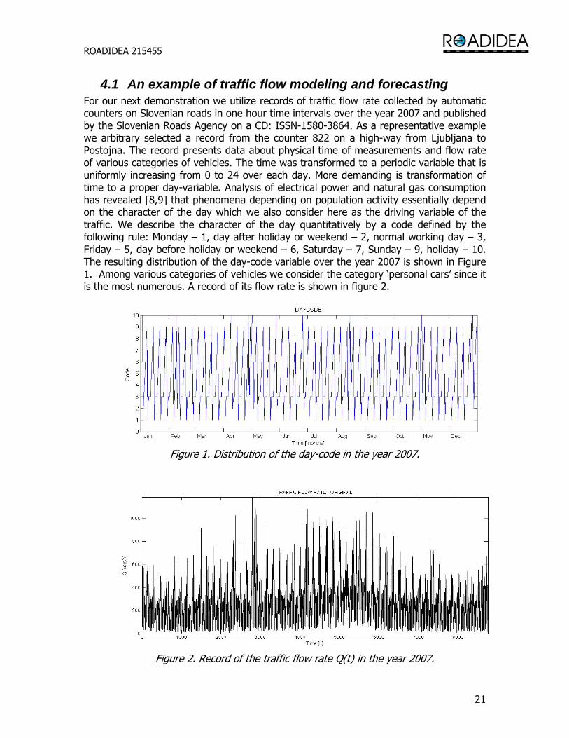
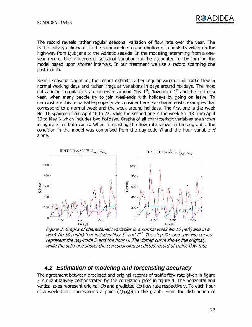
4.1 An example of traffic flow modeling and forecasting For our next demonstration we utilize records of traffic flow rate collected by automatic counters on Slovenian roads in one hour time intervals over the year 2007 and published by the Slovenian Roads Agency on a CD: ISSN-1580-3864. As a representative example we arbitrary selected a record from the counter 822 on a high-way from Ljubljana to Postojna. The record presents data about physical time of measurements and flow rate of various categories of vehicles. The time was transformed to a periodic variable that is uniformly increasing from 0 to 24 over each day. More demanding is transformation of time to a proper day-variable. Analysis of electrical power and natural gas consumption has revealed [8,9] that phenomena depending on population activity essentially depend on the character of the day which we also consider here as the driving variable of the traffic. We describe the character of the day quantitatively by a code defined by the following rule: Monday – 1, day after holiday or weekend – 2, normal working day – 3, Friday – 5, day before holiday or weekend – 6, Saturday – 7, Sunday – 9, holiday – 10. The resulting distribution of the day-code variable over the year 2007 is shown in Figure 1. Among various categories of vehicles we consider the category ‘personal cars’ since it is the most numerous. A record of its flow rate is shown in figure 2.

Figure 1. Distribution of the day-code in the year 2007.

Figure 2. Record of the traffic flow rate Q(t) in the year 2007.

ROADIDEA 215455

22

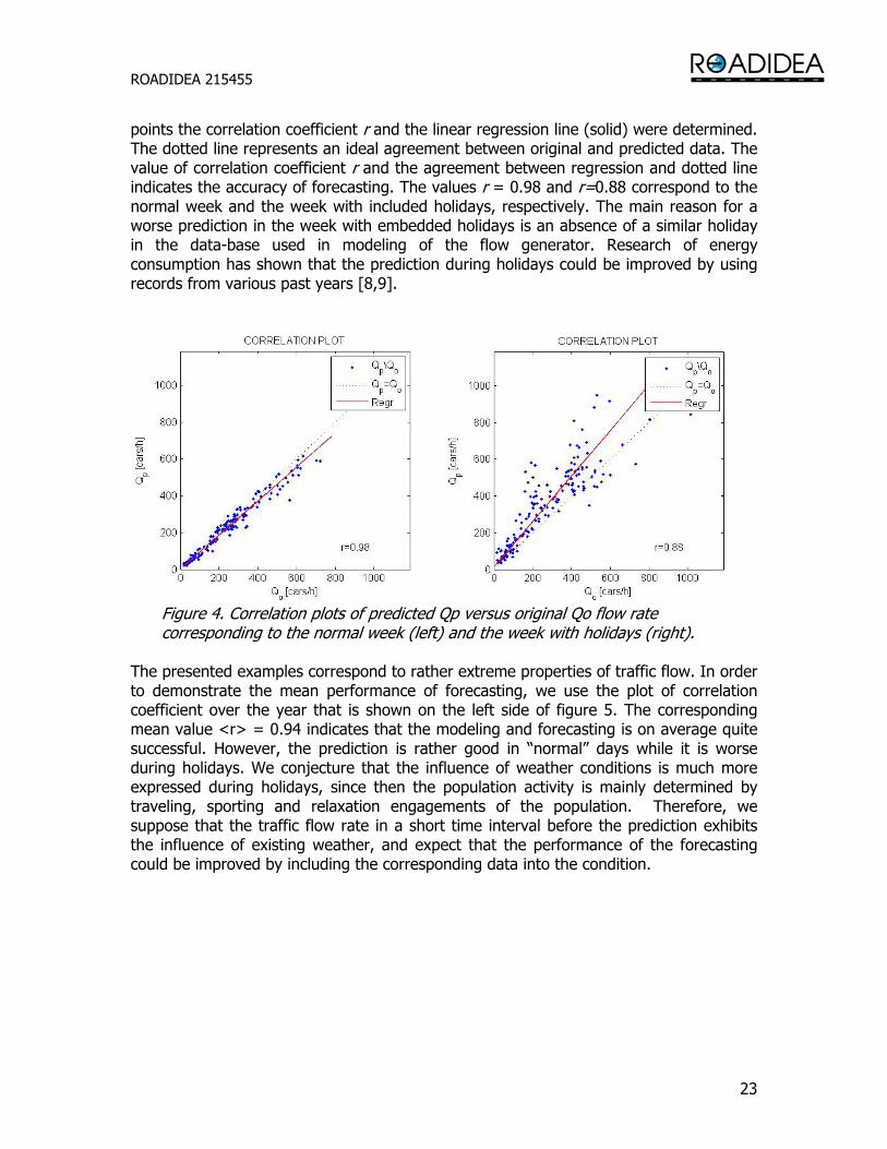
The record reveals rather regular seasonal variation of flow rate over the year. The traffic activity culminates in the summer due to contribution of tourists traveling on the high-way from Ljubljana to the Adriatic seaside. In the modeling, stemming from a one-year record, the influence of seasonal variation can be accounted for by forming the model based upon shorter intervals. In our treatment we use a record spanning one past month. Beside seasonal variation, the record exhibits rather regular variation of traffic flow in normal working days and rather irregular variations in days around holidays. The most outstanding irregularities are observed around May 1st, November 1st and the end of a year, when many people try to join weekends with holidays by going on leave. To demonstrate this remarkable property we consider here two characteristic examples that correspond to a normal week and the week around holidays. The first one is the week No. 16 spanning from April 16 to 22, while the second one is the week No. 18 from April 30 to May 6 which includes two holidays. Graphs of all characteristic variables are shown in figure 3 for both cases. When forecasting the flow rate shown in these graphs, the condition in the model was comprised from the day-code D and the hour variable H alone.

Figure 3. Graphs of characteristic variables in a normal week No.16 (left) and in a week No.18 (right) that includes May 1st and 2nd. The step-like and saw-like curves represent the day-code D and the hour H. The dotted curve shows the original, while the solid one shows the corresponding predicted record of traffic flow rate.

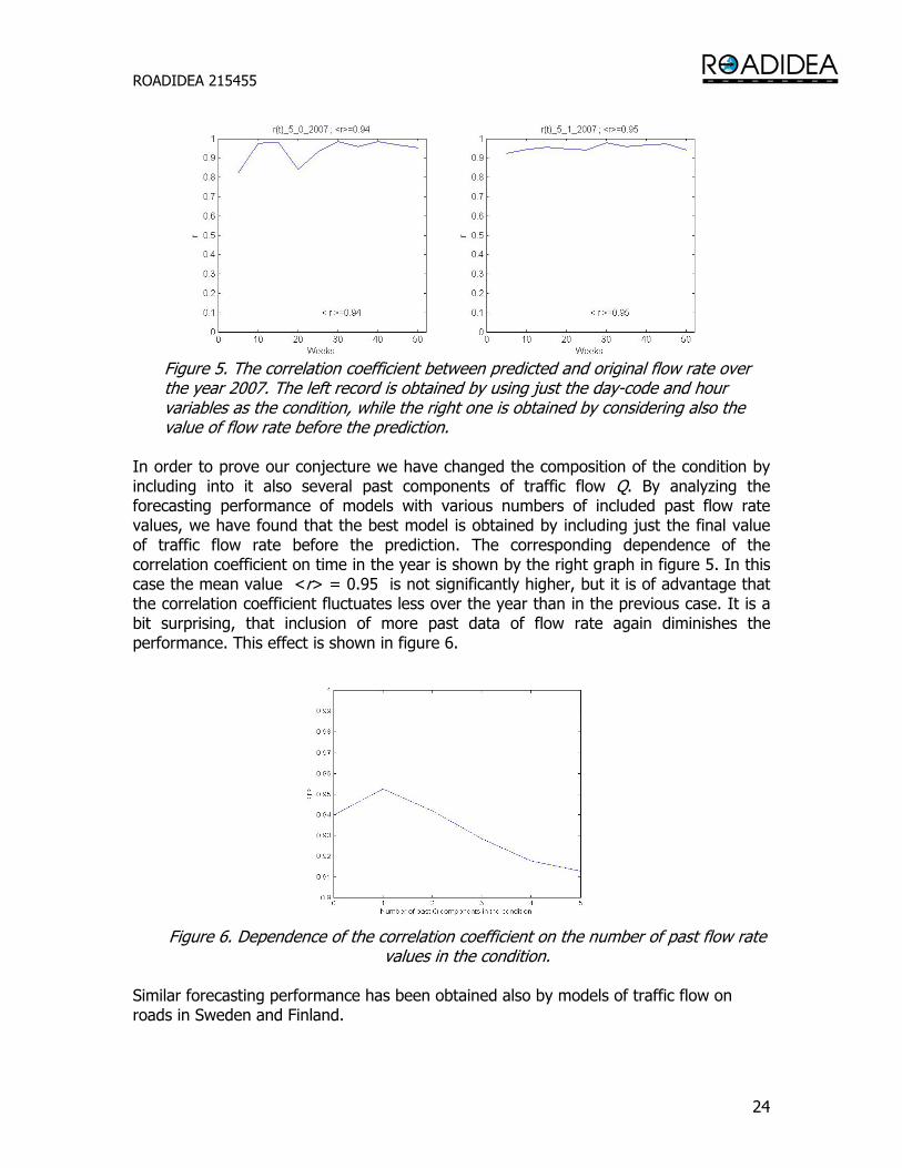
4.2 Estimation of modeling and forecasting accuracy The agreement between predicted and original records of traffic flow rate given in figure 3 is quantitatively demonstrated by the correlation plots in figure 4. The horizontal and vertical axes represent original Qo and predicted Qp flow rate respectively. To each hour of a week there corresponds a point (Qo,Qp) in the graph. From the distribution of

ROADIDEA 215455

23

points the correlation coefficient r and the linear regression line (solid) were determined. The dotted line represents an ideal agreement between original and predicted data. The value of correlation coefficient r and the agreement between regression and dotted line indicates the accuracy of forecasting. The values r = 0.98 and r=0.88 correspond to the normal week and the week with included holidays, respectively. The main reason for a worse prediction in the week with embedded holidays is an absence of a similar holiday in the data-base used in modeling of the flow generator. Research of energy consumption has shown that the prediction during holidays could be improved by using records from various past years [8,9].

Figure 4. Correlation plots of predicted Qp versus original Qo flow rate corresponding to the normal week (left) and the week with holidays (right).

The presented examples correspond to rather extreme properties of traffic flow. In order to demonstrate the mean performance of forecasting, we use the plot of correlation coefficient over the year that is shown on the left side of figure 5. The corresponding mean value <r> = 0.94 indicates that the modeling and forecasting is on average quite successful. However, the prediction is rather good in “normal” days while it is worse during holidays. We conjecture that the influence of weather conditions is much more expressed during holidays, since then the population activity is mainly determined by traveling, sporting and relaxation engagements of the population. Therefore, we suppose that the traffic flow rate in a short time interval before the prediction exhibits the influence of existing weather, and expect that the performance of the forecasting could be improved by including the corresponding data into the condition.

ROADIDEA 215455

24

Figure 5. The correlation coefficient between predicted and original flow rate over the year 2007. The left record is obtained by using just the day-code and hour variables as the condition, while the right one is obtained by considering also the value of flow rate before the prediction.

In order to prove our conjecture we have changed the composition of the condition by including into it also several past components of traffic flow Q. By analyzing the forecasting performance of models with various numbers of included past flow rate values, we have found that the best model is obtained by including just the final value of traffic flow rate before the prediction. The corresponding dependence of the correlation coefficient on time in the year is shown by the right graph in figure 5. In this case the mean value <r> = 0.95 is not significantly higher, but it is of advantage that the correlation coefficient fluctuates less over the year than in the previous case. It is a bit surprising, that inclusion of more past data of flow rate again diminishes the performance. This effect is shown in figure 6.

Figure 6. Dependence of the correlation coefficient on the number of past flow rate

values in the condition. Similar forecasting performance has been obtained also by models of traffic flow on roads in Sweden and Finland.

ROADIDEA 215455

25

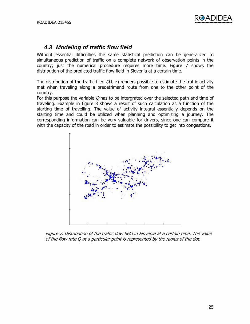
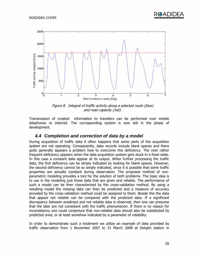
4.3 Modeling of traffic flow field Without essential difficulties the same statistical prediction can be generalized to simultaneous prediction of traffic on a complete network of observation points in the country; just the numerical procedure requires more time. Figure 7 shows the distribution of the predicted traffic flow field in Slovenia at a certain time. The distribution of the traffic filed Q(t, r) renders possible to estimate the traffic activity met when traveling along a predetrimend route from one to the other point of the country. For this purpose the variable Q has to be intergrated over the selected path and time of traveling. Example in figure 8 shows a result of such calculation as a function of the starting time of travelling. The value of activity integral essentially depends on the starting time and could be utilized when planning and optimizing a journey. The corresponding information can be very valuable for drivers, since one can compare it with the capacity of the road in order to estimate the possibility to get into congestions.

Figure 7. Distribution of the traffic flow field in Slovenia at a certain time. The value of the flow rate Q at a particular point is represented by the radius of the dot.

ROADIDEA 215455

26

Figure 8. Integral of traffic activity along a selected route (blue)

and road capacity (red). Transmission of created information to travellers can be performed over mobile telephones or internet. The corresponding system is now still in the phase of development.

4.4 Completion and correction of data by a model During acquisition of traffic data it often happens that some parts of the acquisition system are not operating. Consequently, data records include blank spaces and there quite generally appears a problem how to overcome this deficiency. The next rather frequent deficiency appears when the data acquisition system gets stuck in a fixed state. In this case a constant data appear at its output. When further processing the traffic data, the first deficiency can be simply indicated by looking for blank spaces. However, the second deficiency cannot be so simply indicated, since it is possible that some traffic properties are actually constant during observation. The proposed method of non-parametric modeling provides a tool for the solution of both problems. The basic idea is to use in the modeling just those data that are given and reliable. The performance of such a model can be then characterized by the cross-validation method. By using a resulting model the missing data can then be predicted and a measure of accuracy provided by the cross-validation method could be assigned to them. Beside this the data that appear not reliable can be compared with the predicted data. If a significant discrepancy between predicted and not reliable data is observed, then one can presume that the later are not consistent with the traffic phenomenon. If there is no reason for inconsistency one could conjecture that non-reliable data should also be substituted by predicted ones, or at least somehow indicated by a parameter of reliability. In order to demonstrate such a treatment we utilize an example of data provided by traffic observation from 1 November 2007 to 31 March 2008 at Delsjön station in

ROADIDEA 215455

27

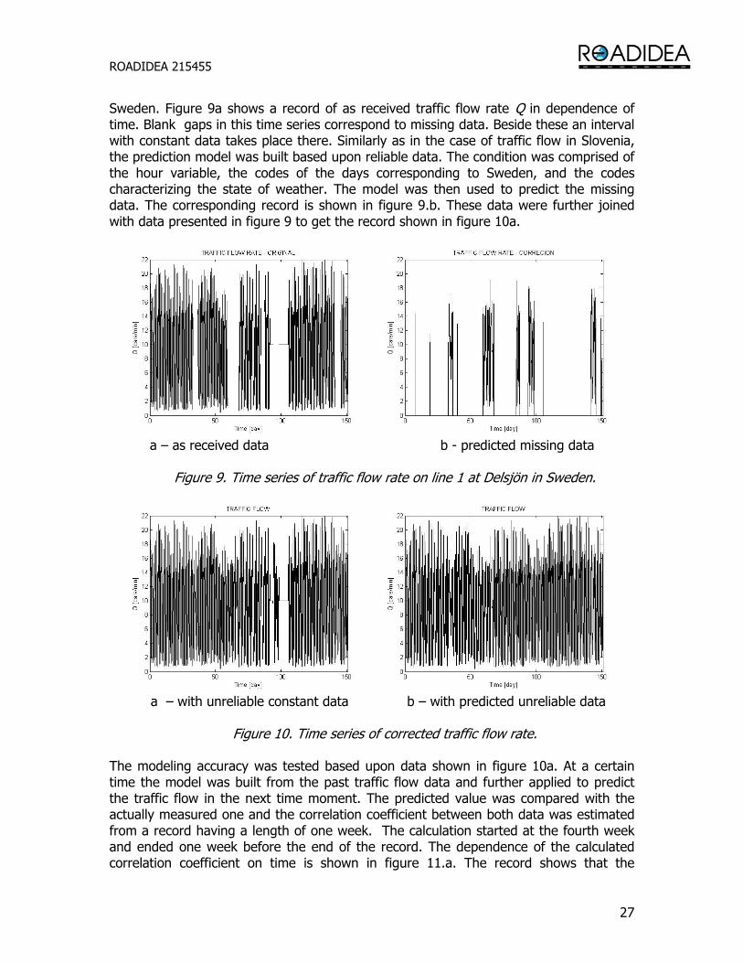
Sweden. Figure 9a shows a record of as received traffic flow rate Q in dependence of time. Blank gaps in this time series correspond to missing data. Beside these an interval with constant data takes place there. Similarly as in the case of traffic flow in Slovenia, the prediction model was built based upon reliable data. The condition was comprised of the hour variable, the codes of the days corresponding to Sweden, and the codes characterizing the state of weather. The model was then used to predict the missing data. The corresponding record is shown in figure 9.b. These data were further joined with data presented in figure 9 to get the record shown in figure 10a.

a – as received data b - predicted missing data

Figure 9. Time series of traffic flow rate on line 1 at Delsjön in Sweden.

a – with unreliable constant data b – with predicted unreliable data

Figure 10. Time series of corrected traffic flow rate.

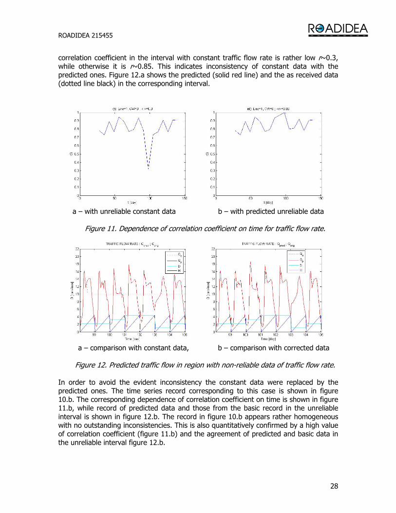
The modeling accuracy was tested based upon data shown in figure 10a. At a certain time the model was built from the past traffic flow data and further applied to predict the traffic flow in the next time moment. The predicted value was compared with the actually measured one and the correlation coefficient between both data was estimated from a record having a length of one week. The calculation started at the fourth week and ended one week before the end of the record. The dependence of the calculated correlation coefficient on time is shown in figure 11.a. The record shows that the

ROADIDEA 215455

28

correlation coefficient in the interval with constant traffic flow rate is rather low r~0.3, while otherwise it is r~0.85. This indicates inconsistency of constant data with the predicted ones. Figure 12.a shows the predicted (solid red line) and the as received data (dotted line black) in the corresponding interval.

a – with unreliable constant data b – with predicted unreliable data

Figure 11. Dependence of correlation coefficient on time for traffic flow rate.

a – comparison with constant data, b – comparison with corrected data

Figure 12. Predicted traffic flow in region with non-reliable data of traffic flow rate.

In order to avoid the evident inconsistency the constant data were replaced by the predicted ones. The time series record corresponding to this case is shown in figure 10.b. The corresponding dependence of correlation coefficient on time is shown in figure 11.b, while record of predicted data and those from the basic record in the unreliable interval is shown in figure 12.b. The record in figure 10.b appears rather homogeneous with no outstanding inconsistencies. This is also quantitatively confirmed by a high value of correlation coefficient (figure 11.b) and the agreement of predicted and basic data in the unreliable interval figure 12.b.

ROADIDEA 215455

29

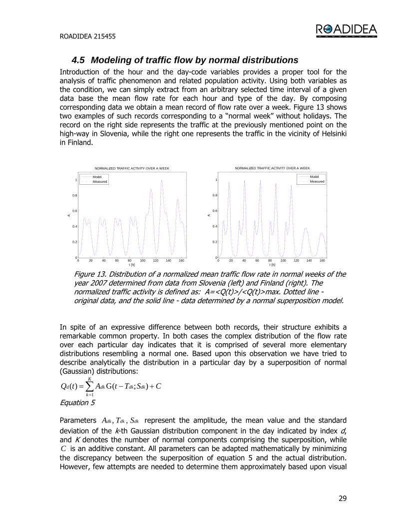
4.5 Modeling of traffic flow by normal distributions Introduction of the hour and the day-code variables provides a proper tool for the analysis of traffic phenomenon and related population activity. Using both variables as the condition, we can simply extract from an arbitrary selected time interval of a given data base the mean flow rate for each hour and type of the day. By composing corresponding data we obtain a mean record of flow rate over a week. Figure 13 shows two examples of such records corresponding to a “normal week” without holidays. The record on the right side represents the traffic at the previously mentioned point on the high-way in Slovenia, while the right one represents the traffic in the vicinity of Helsinki in Finland.

0 20 40 60 80 100 120 140 1600

0.2

0.4

0.6

0.8

1

t [h]

A

NORMALIZED TRAFFIC ACTIVITY OVER A WEEK

ModelMeasured

0 20 40 60 80 100 120 140 1600

0.2

0.4

0.6

0.8

1

t [h]

A

NORMALIZED TRAFFIC ACTIVITY OVER A WEEK

ModelMeasured

Figure 13. Distribution of a normalized mean traffic flow rate in normal weeks of the year 2007 determined from data from Slovenia (left) and Finland (right). The normalized traffic activity is defined as: A=<Q(t)>/<Q(t)>max. Dotted line - original data, and the solid line - data determined by a normal superposition model.

In spite of an expressive difference between both records, their structure exhibits a remarkable common property. In both cases the complex distribution of the flow rate over each particular day indicates that it is comprised of several more elementary distributions resembling a normal one. Based upon this observation we have tried to describe analytically the distribution in a particular day by a superposition of normal (Gaussian) distributions:

CSTtAtQ dkdk

K

kdkd +−= ∑

=

);(G)(1

Equation 5 Parameters dkdkdk STA ,, represent the amplitude, the mean value and the standard deviation of the k-th Gaussian distribution component in the day indicated by index d, and K denotes the number of normal components comprising the superposition, while C is an additive constant. All parameters can be adapted mathematically by minimizing the discrepancy between the superposition of equation 5 and the actual distribution. However, few attempts are needed to determine them approximately based upon visual

ROADIDEA 215455

30

inspection of a given record. According to this, we have found the following parameters of the superposition for both characteristic examples.

Parameters of normal superposition for data from Slovenia Parameter values: T1=9.9h, T2=17.6h, S1=2.7h, S2=3.1h, C=0.03 are constant while amplitudes are variable, as shown in Table 2.

ROADIDEA 215455

31

Mon Tue Wed Thu Fri Sat Sun

A1 1.0 1.0 1.0 1.0 1.0 2.0 1.5

A2 1.0 1.0 1.0 1.0 1.8 1.1 0.9

Table 2. Amplitudes of normal superposition for data from Slovenia.

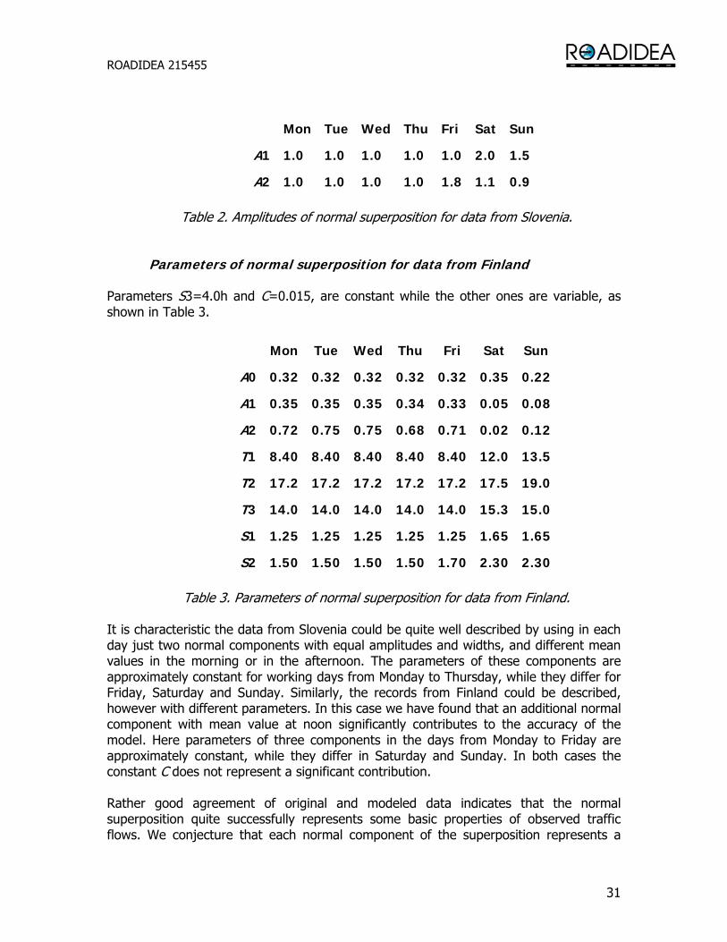
Parameters of normal superposition for data from Finland Parameters S3=4.0h and C=0.015, are constant while the other ones are variable, as shown in Table 3.

Mon Tue Wed Thu Fri Sat Sun

A0 0.32 0.32 0.32 0.32 0.32 0.35 0.22

A1 0.35 0.35 0.35 0.34 0.33 0.05 0.08

A2 0.72 0.75 0.75 0.68 0.71 0.02 0.12

T1 8.40 8.40 8.40 8.40 8.40 12.0 13.5

T2 17.2 17.2 17.2 17.2 17.2 17.5 19.0

T3 14.0 14.0 14.0 14.0 14.0 15.3 15.0

S1 1.25 1.25 1.25 1.25 1.25 1.65 1.65

S2 1.50 1.50 1.50 1.50 1.70 2.30 2.30

Table 3. Parameters of normal superposition for data from Finland. It is characteristic the data from Slovenia could be quite well described by using in each day just two normal components with equal amplitudes and widths, and different mean values in the morning or in the afternoon. The parameters of these components are approximately constant for working days from Monday to Thursday, while they differ for Friday, Saturday and Sunday. Similarly, the records from Finland could be described, however with different parameters. In this case we have found that an additional normal component with mean value at noon significantly contributes to the accuracy of the model. Here parameters of three components in the days from Monday to Friday are approximately constant, while they differ in Saturday and Sunday. In both cases the constant C does not represent a significant contribution. Rather good agreement of original and modeled data indicates that the normal superposition quite successfully represents some basic properties of observed traffic flows. We conjecture that each normal component of the superposition represents a

ROADIDEA 215455

32

synchronized activity of some group of population and expect that the corresponding characteristic parameters could be also determined based upon a proper sociological research.

5 Joining of weather and traffic data

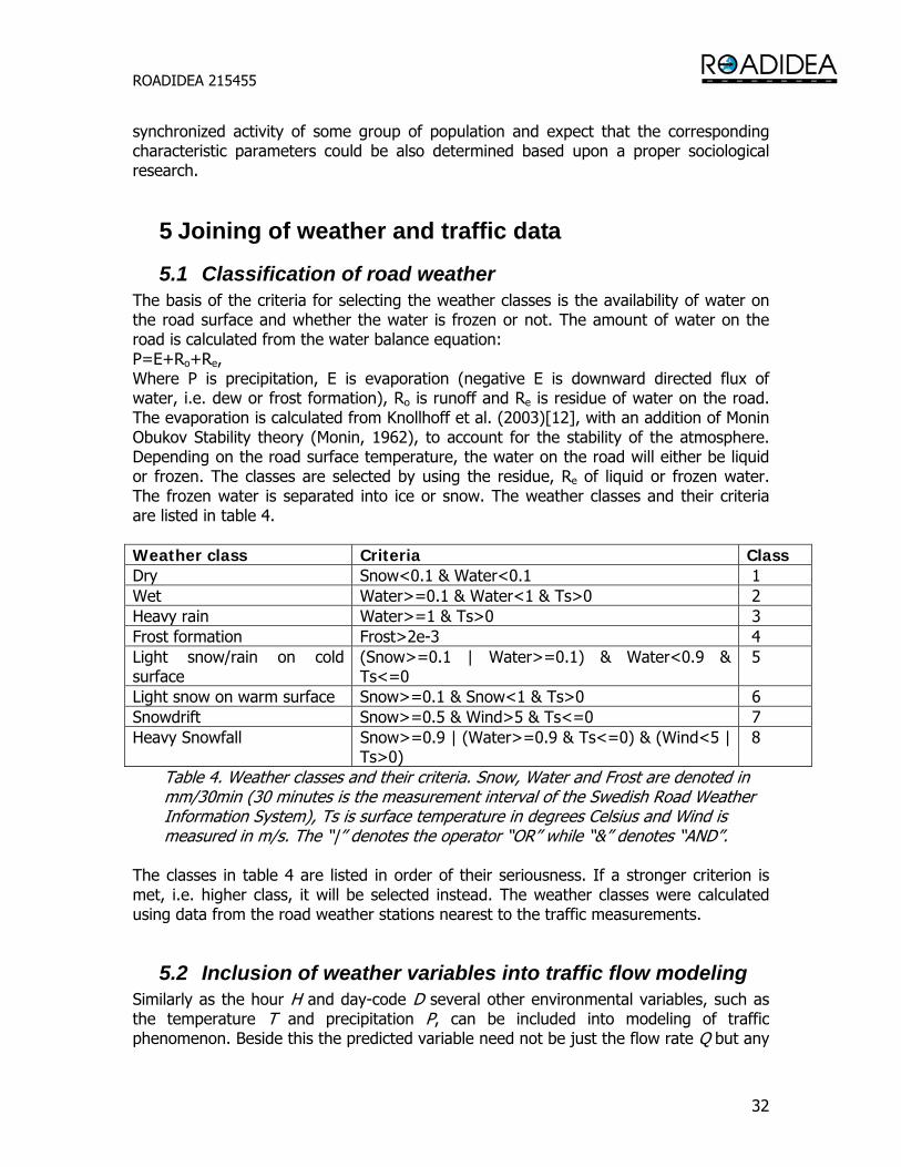
5.1 Classification of road weather The basis of the criteria for selecting the weather classes is the availability of water on the road surface and whether the water is frozen or not. The amount of water on the road is calculated from the water balance equation: P=E+Ro+Re, Where P is precipitation, E is evaporation (negative E is downward directed flux of water, i.e. dew or frost formation), Ro is runoff and Re is residue of water on the road. The evaporation is calculated from Knollhoff et al. (2003)[12], with an addition of Monin Obukov Stability theory (Monin, 1962), to account for the stability of the atmosphere. Depending on the road surface temperature, the water on the road will either be liquid or frozen. The classes are selected by using the residue, Re of liquid or frozen water. The frozen water is separated into ice or snow. The weather classes and their criteria are listed in table 4. Weather class Criteria Class Dry Snow<0.1 & Water<0.1 1 Wet Water>=0.1 & Water<1 & Ts>0 2 Heavy rain Water>=1 & Ts>0 3 Frost formation Frost>2e-3 4 Light snow/rain on cold surface

(Snow>=0.1 | Water>=0.1) & Water<0.9 & Ts<=0

5

Light snow on warm surface Snow>=0.1 & Snow<1 & Ts>0 6 Snowdrift Snow>=0.5 & Wind>5 & Ts<=0 7 Heavy Snowfall Snow>=0.9 | (Water>=0.9 & Ts<=0) & (Wind<5 |

Ts>0) 8

Table 4. Weather classes and their criteria. Snow, Water and Frost are denoted in mm/30min (30 minutes is the measurement interval of the Swedish Road Weather Information System), Ts is surface temperature in degrees Celsius and Wind is measured in m/s. The “|” denotes the operator “OR” while “&” denotes “AND”.

The classes in table 4 are listed in order of their seriousness. If a stronger criterion is met, i.e. higher class, it will be selected instead. The weather classes were calculated using data from the road weather stations nearest to the traffic measurements.

5.2 Inclusion of weather variables into traffic flow modeling Similarly as the hour H and day-code D several other environmental variables, such as the temperature T and precipitation P, can be included into modeling of traffic phenomenon. Beside this the predicted variable need not be just the flow rate Q but any

ROADIDEA 215455

33

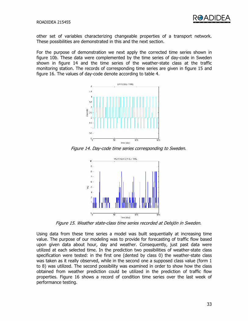
other set of variables characterizing changeable properties of a transport network. These possibilities are demonstrated in this and the next section. For the purpose of demonstration we next apply the corrected time series shown in figure 10b. These data were complemented by the time series of day-code in Sweden shown in figure 14 and the time series of the weather-state class at the traffic monitoring station. The records of corresponding time series are given in figure 15 and figure 16. The values of day-code denote according to table 4.

Figure 14. Day-code time series corresponding to Sweden.

Figure 15. Weather state-class time series recorded at Delsjön in Sweden.

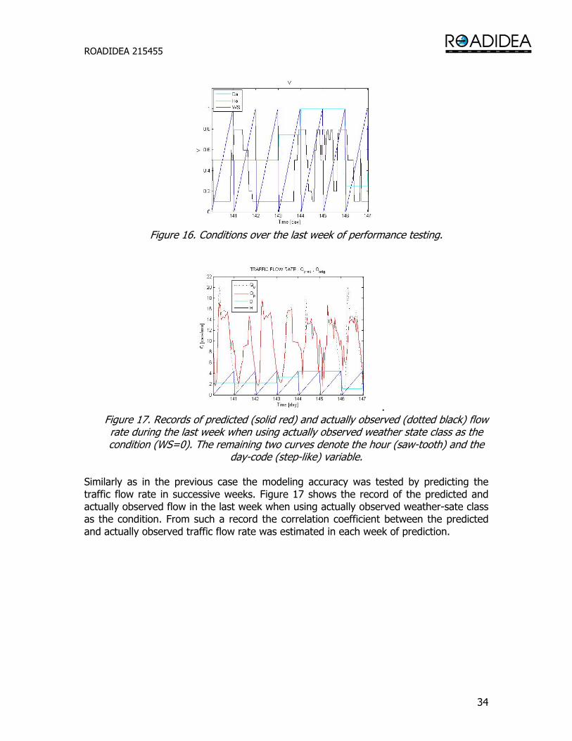
Using data from these time series a model was built sequentially at increasing time value. The purpose of our modeling was to provide for forecasting of traffic flow based upon given data about hour, day and weather. Consequently, just past data were utilized at each selected time. In the prediction two possibilities of weather-state class specification were tested: in the first one (dented by class 0) the weather-state class was taken as it really observed, while in the second one a supposed class value (form 1 to 8) was utilized. The second possibility was examined in order to show how the class obtained from weather prediction could be utilized in the prediction of traffic flow properties. Figure 16 shows a record of condition time series over the last week of performance testing.

ROADIDEA 215455

34

Figure 16. Conditions over the last week of performance testing.

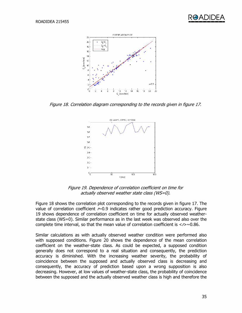
. Figure 17. Records of predicted (solid red) and actually observed (dotted black) flow rate during the last week when using actually observed weather state class as the condition (WS=0). The remaining two curves denote the hour (saw-tooth) and the

day-code (step-like) variable.

Similarly as in the previous case the modeling accuracy was tested by predicting the traffic flow rate in successive weeks. Figure 17 shows the record of the predicted and actually observed flow in the last week when using actually observed weather-sate class as the condition. From such a record the correlation coefficient between the predicted and actually observed traffic flow rate was estimated in each week of prediction.

ROADIDEA 215455

35

Figure 18. Correlation diagram corresponding to the records given in figure 17.

Figure 19. Dependence of correlation coefficient on time for actually observed weather state class (WS=0).

Figure 18 shows the correlation plot corresponding to the records given in figure 17. The value of correlation coefficient r~0.9 indicates rather good prediction accuracy. Figure 19 shows dependence of correlation coefficient on time for actually observed weather-state class (WS=0). Similar performance as in the last week was observed also over the complete time interval, so that the mean value of correlation coefficient is <r>~0.86. Similar calculations as with actually observed weather condition were performed also with supposed conditions. Figure 20 shows the dependence of the mean correlation coefficient on the weather-state class. As could be expected, a supposed condition generally does not correspond to a real situation and consequently, the prediction accuracy is diminished. With the increasing weather severity, the probability of coincidence between the supposed and actually observed class is decreasing and consequently, the accuracy of prediction based upon a wrong supposition is also decreasing. However, at low values of weather-state class, the probability of coincidence between the supposed and the actually observed weather class is high and therefore the

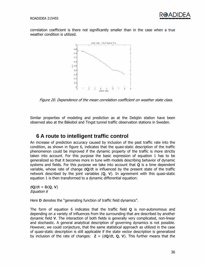
ROADIDEA 215455

36

correlation coefficient is there not significantly smaller than in the case when a true weather condition is utilized.

Figure 20. Dependence of the mean correlation coefficient on weather state class.

Similar properties of modeling and prediction as at the Delsjön station have been observed also at the Bäkebol and Tingst tunnel traffic observation stations in Sweden.

6 A route to intelligent traffic control An increase of prediction accuracy caused by inclusion of the past traffic rate into the condition, as shown in figure 6, indicates that the quasi-static description of the traffic phenomenon could be improved if the dynamic property of the traffic is more strictly taken into account. For this purpose the basic expression of equation 1 has to be generalized so that it becomes more in tune with models describing behavior of dynamic systems and fields. For this purpose we take into account that Q is a time dependent variable, whose rate of change dQ/dt is influenced by the present state of the traffic network described by the joint variables (Q, V). In agreement with this quasi-static equation 1 is then transformed to a dynamic differential equation: dQ/dt = D(Q, V) Equation 6 Here D denotes the “generating function of traffic field dynamics”. The form of equation 6 indicates that the traffic field Q is non-autonomous and depending on a variety of influences from the surrounding that are described by another dynamic field V. The interaction of both fields is generally very complicated, non-linear and stochastic. A general analytical description of governing dynamics is not possible. However, we could conjecture, that the same statistical approach as utilized in the case of quasi-static description is still applicable if the state vector description is generalized by inclusion of the rate of changes: Z = (dQ/dt, Q, V). This further means that the

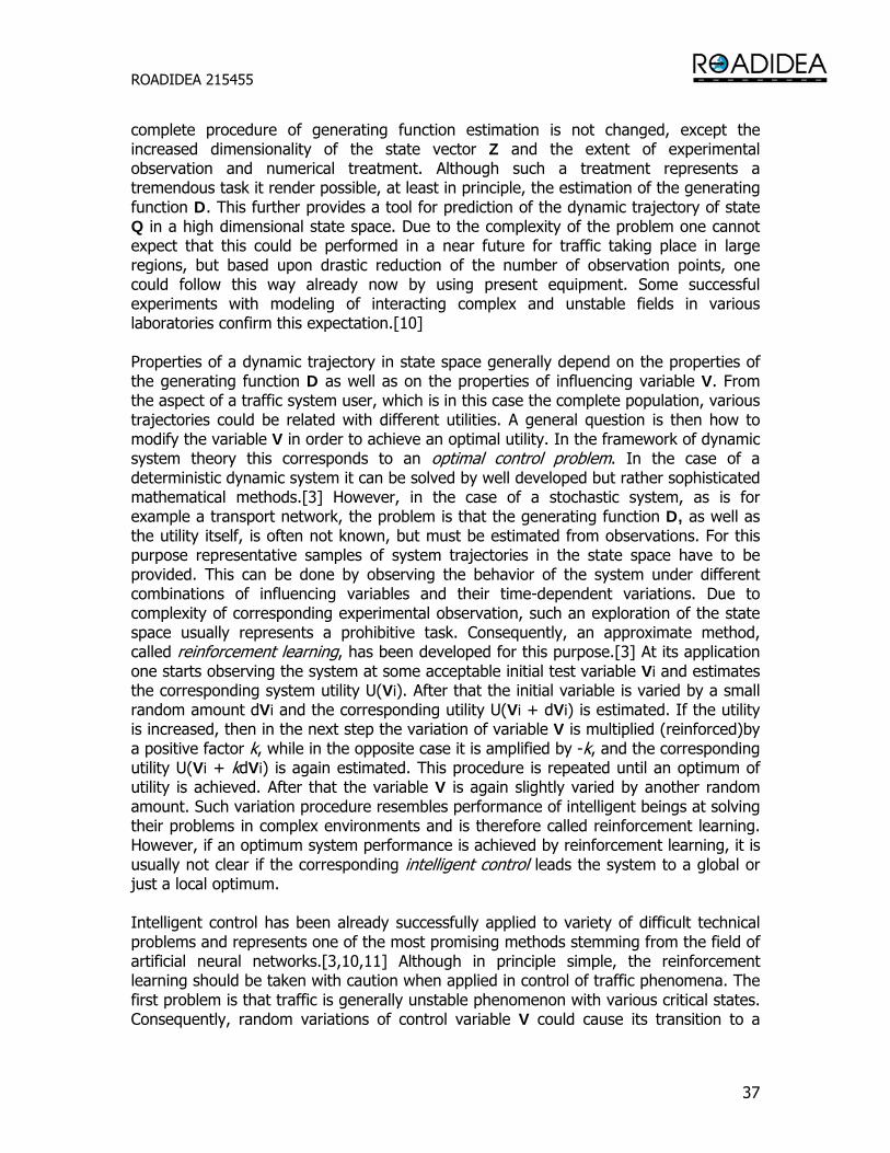
ROADIDEA 215455

37

complete procedure of generating function estimation is not changed, except the increased dimensionality of the state vector Z and the extent of experimental observation and numerical treatment. Although such a treatment represents a tremendous task it render possible, at least in principle, the estimation of the generating function D. This further provides a tool for prediction of the dynamic trajectory of state Q in a high dimensional state space. Due to the complexity of the problem one cannot expect that this could be performed in a near future for traffic taking place in large regions, but based upon drastic reduction of the number of observation points, one could follow this way already now by using present equipment. Some successful experiments with modeling of interacting complex and unstable fields in various laboratories confirm this expectation.[10] Properties of a dynamic trajectory in state space generally depend on the properties of the generating function D as well as on the properties of influencing variable V. From the aspect of a traffic system user, which is in this case the complete population, various trajectories could be related with different utilities. A general question is then how to modify the variable V in order to achieve an optimal utility. In the framework of dynamic system theory this corresponds to an optimal control problem. In the case of a deterministic dynamic system it can be solved by well developed but rather sophisticated mathematical methods.[3] However, in the case of a stochastic system, as is for example a transport network, the problem is that the generating function D, as well as the utility itself, is often not known, but must be estimated from observations. For this purpose representative samples of system trajectories in the state space have to be provided. This can be done by observing the behavior of the system under different combinations of influencing variables and their time-dependent variations. Due to complexity of corresponding experimental observation, such an exploration of the state space usually represents a prohibitive task. Consequently, an approximate method, called reinforcement learning, has been developed for this purpose.[3] At its application one starts observing the system at some acceptable initial test variable Vi and estimates the corresponding system utility U(Vi). After that the initial variable is varied by a small random amount dVi and the corresponding utility U(Vi + dVi) is estimated. If the utility is increased, then in the next step the variation of variable V is multiplied (reinforced)by a positive factor k, while in the opposite case it is amplified by -k, and the corresponding utility U(Vi + kdVi) is again estimated. This procedure is repeated until an optimum of utility is achieved. After that the variable V is again slightly varied by another random amount. Such variation procedure resembles performance of intelligent beings at solving their problems in complex environments and is therefore called reinforcement learning. However, if an optimum system performance is achieved by reinforcement learning, it is usually not clear if the corresponding intelligent control leads the system to a global or just a local optimum. Intelligent control has been already successfully applied to variety of difficult technical problems and represents one of the most promising methods stemming from the field of artificial neural networks.[3,10,11] Although in principle simple, the reinforcement learning should be taken with caution when applied in control of traffic phenomena. The first problem is that traffic is generally unstable phenomenon with various critical states. Consequently, random variations of control variable V could cause its transition to a

ROADIDEA 215455

38

critical state. Beside this, in the case of traffic, we generally deal with fields, and hence variation of external variables requires tremendous number of trials.

7 Summary and conclusions In this chapter of the report the focus is on a description of general statistical methods of traffic modeling. Hence, only non-parametric statistical approach has been considered, while specific parametric methods have been omitted. Similarly, description of problems related with adaptation of the proposed methods to specific information processing and transmission devices and estimation of information cost have also been omitted. Since the complete non-parametric model stems from recorded data it is rather generally applicable. In spite of the complexity of roads traffic phenomena, non-parametric statistical modeling of relations between characteristic variables by conditional average estimator appears quite promising for generation of new information. Demonstrated examples indicate that this method can be simply utilized in prediction of traffic field distribution and related variables such as integral of traffic activity and an optimal traveling time interval. It could also provide information about possibility of congestion development in the selected traveling time interval, etc. Beside this, non-parametric approach renders possible a simple joining of weather and traffic data and related prediction of critical states. The information generated by such a treatment can be simply transmitted to participants in the traffic over existing communication devices such as mobile telephones or internet. An important advantage of non-parametric statistical modeling is that the governing algorithm can be formulated rather generally and executed practically automatically without essential modification at its adaptation to a specific case. It also permits a simple inclusion of control variables into the description. Consequently, the non-parametric statistical modeling provides also a basis for an optimal control of traffic. However, its true application still requires additional research.

8 References [1] D. Helbing, Verkehrsdynamik, Springer, Berlin, 1997. [2] B. S. Kerner, The Physics of Traffic, Springer, Berlin, 2004. [3] I. Grabec, W. Sachse, Synergetics of Measurements, Prediction, and Control, Springer, Berlin. 1997 [4] I. Grabec, K. Kalcher, F. Švegl, Modelling and Forecasting of Traffic Flow on Slovenian High-Ways, Proc. of the conf.: Transport Research Arena Europe 2008”, Ljubljana, SI, April 21-24, 2008, ISBN 978-961-6527-12-5 (DRC) [5] I. Grabec, K. Kalcher, F. Švegl, Statistical Forecasting of Traffic Flow Rate, Proc. of the 14th Int. Road Weather Conf. 2008”, Prague, CzR, May 14-16, 2008, ID 50, ISBN 978-80-87205-01-3, disc published by Wirelesscom, www.sirwec.cz

ROADIDEA 215455

39

[6] I. Grabec, Experimental modelling of physical laws, Eur. Phys. J. B 22, 129-135 (2001). [7] I. Grabec, Extraction of physical laws from joint experimental data, Eur. Phys. J. B 48, 279-286 (2005). [8] B. Lunar, I. Grabec. Forecasting Electrical Power Consumption by Normalised Radial Basis Function Neural Network, Neural Network World, 12(3), 241-254 (2002) [9] M., Thaler, I. Grabec, A. Poredoš. Prediction of Energy Consumption and Risk of Excess Demand in a Distribution System, Physica A: Stat. Mech. & Applications, 355(1), 46-53 (2005). [10] Several references of interest for non-parametric statistical modeling of complex physical laws are available at web page of I. Grabec: http://www.fs.uni-lj.si [11] Handbook of Intelligent Control, Neural, Fuzzy and Adaptive Approaches, Eds.: D. A. White, D. A. Sofge, Van Nostrand Reinhold, New York 1992 [12] Knollhoff, D. S., E. S. Tackle, W. A. Gallus Jr., D. Burckheimer D. McCauley, 2003: Evaluation of a frost accumulation model. Meteor. Appl., 10, 337–343. Acknowledgement

The authors would like to thank the Slovenian Agency for Roads, and especially Mrs. Tatjana Bubnič for preparation of flow rate data. Data from Finland were provided by Ari Sirkiä from VTT – Technical Research Centre of Finland. Data from Sweden were provided by Roadidea Partners Semcon and Klimator.