Embed Size (px)
Citation preview

Master’s Thesis
Road Safety and Adverse Weather ConditionsAn empirical analysis of speeding behavior under wet pavement conditions
Submitted at theFaculty of Business, Economics and Social Sciences
University of Bern
Institute of Business Management and MarketingSection Consumer Behavior
SupervisorDr. Michael Schulte-Mecklenbeck
Submitted byAuthor: Ozan Harman
Student ID: 08-926-305Address: Muhlemattstrasse 59
3007 BernPlace of origin: Zurich, ZH
E-Mail: [email protected] of Submission: September 13, 2016

Abstract
Precipitation is known to increase traffic accidents and fatalities.
However, it is not fully understood how precipitation impact driver
behavior. This study examined how drivers’ adapt speed to changes
from dry to wet pavement conditions. Speed and pavement condition
were evaluated using radar data and surveillance images in a speed
limit 50 km/h two way road section in Zurich, Switzerland. The total
sample consisted of 195’799 vehicles and 7’988 images for the entire
month of February, 2016. To balance our sample we matched pairs by
day, hour, congestion, and hour category (for weekdays). Using the
wilcoxon signed rank test and the fligner-killeen variance homogeneity
test we analyzed speed median and dispersion for differences between
dry and wet pavement conditions. We found that a change from dry
to wet pavement conditions induce drivers’ to reduce speed by 2.7-
5.4 percent. For speed dispersion the results are less consistent; for
weekends and weekday middays dispersion did not differ, whereas dis-
persion differed for weekday mornings and evenings between dry and
wet conditions. Finally, we found that drivers’ do not reduce speed
sufficiently to have equal braking distances in dry and wet conditions.
2

Acknowledgement
First and foremost, I would like to express my gratitude to my supervisor
Dr. Michael Schulte-Mecklenbeck, who competently guided me and granted
me the freedom to explore the topics I was interested in.
I am also grateful to my dear friend, David Wartmann and my father in
law, Olivier Peter for their insightful comments and encouragement on those
scientifically dark days.
My parents supported me wherever possible during my whole life and enabled
me to pursue my education. They deserve my sincere gratitude.
Last but not least, my sincere thanks also goes to Audrey Peter for her loving
support, attention and encouragements.
3

Contents
1 Introduction 6
1.1 Problem Statement . . . . . . . . . . . . . . . . . . . . . . . . 7
2 Overview 8
2.1 Road Safety . . . . . . . . . . . . . . . . . . . . . . . . . . . . 8
2.2 Driver Behavior . . . . . . . . . . . . . . . . . . . . . . . . . . 12
2.3 Rain and Traffic . . . . . . . . . . . . . . . . . . . . . . . . . . 15
2.4 Research Question and Hypothesis . . . . . . . . . . . . . . . 18
3 Methodology 19
3.1 Site Characteristics . . . . . . . . . . . . . . . . . . . . . . . . 19
3.2 Traffic Data . . . . . . . . . . . . . . . . . . . . . . . . . . . . 19
3.3 Weather Data . . . . . . . . . . . . . . . . . . . . . . . . . . . 21
4 Results 23
4.1 Data Preparation . . . . . . . . . . . . . . . . . . . . . . . . . 23
4.2 Subsetting Data . . . . . . . . . . . . . . . . . . . . . . . . . . 24
4.3 Matching . . . . . . . . . . . . . . . . . . . . . . . . . . . . . 25
4.4 Hypothesis Testing . . . . . . . . . . . . . . . . . . . . . . . . 29
5 Conclusion and Discussion 33
5.1 Causal Chain Model and the Haddon Matrix . . . . . . . . . . 33
5.2 Strengths and weaknesses . . . . . . . . . . . . . . . . . . . . 39
5.3 Directions for Future Research . . . . . . . . . . . . . . . . . . 41
4

Appendix A 42
References 48
List of Tables 54
List of Figures 54
5

1 Introduction
Along with driver attributes many factors impact the probability of traffic
accidents. Environmental factors such as visibility, road design, weather, and
vehicle attributes interact with driver behavior (Tiwari et al., 2005). It is
widely accepted that increased vehicle speed, speed dispersion, and adverse
weather conditions – such as road slipperiness – increase traffic accident prob-
abilities (Brodsky & Hakkert, 1988; Sabey & Staughton, 1975; Almqvist &
Heinig, 2013; Aarts & Van Schagen, 2006; Garber & Gadirau, 1988), therefore
it is important to understand how changes in weather and road conditions
influence driver behavior. Speed alone merely causes an accident; speeding,
speed dispersion, and adverse weather on the other hand are a deadly mix-
ture. Accordingly, pavement conditions are of special interest because they
have a direct measurable influence on vehicle performance. Hamilton (2012)
demonstrated the significance of pavement condition regarding road safety
and showed that the majority of weather induced accidents are related to
wet road surfaces.
Over the past two decades, researchers in this field were challenged regarding
validity, replicability, and accuracy. There is no best way to find an appro-
priate proxy for weather or a preferable measurement method. and (Brodsky
& Hakkert, 1988; Jagerbrand & Sjobergh, 2016; Edwards, 1999).
1) We address accuracy and replicability problems by using raw data from
automated measurements. 2) Previous findings show that adverse weather
conditions such as rainfall measured at nearby weather station lead to higher
accident rates and reduced speeding.
6

We add to this by collecting our data – including our weather data – at
a single study site and by focusing on road surface wetness rather than on
precipitation. 3) Finally, to best of our knowledge there exists no similar
study in Switzerland. This location is of special interest because Switzerland
in line with Sweden is considered to be the safest driving environment world-
wide (BITRE, 2015). Nevertheless road safety needs to be improved since
wet road surface is the most frequent weather related cause of accidents in
Switzerland (ASTRA, 2016).
1.1 Problem Statement
It is commonly accepted that adverse weather conditions increase accident
risk. However, findings in road safety research show flaws regarding study
design, data quality, and methodology (Hauer, 2002). One issue is that
covariates indicating weather condition are based on measurements of nearby
weather stations. This leads to uncertainty about validity – ex post it can’t
be proven if the weather was identical at the different measurement locations.
Further it is loose to assume that a driver’s weather perception is identical
with measurements from a weather station. We solve this problem generating
our weather variable using images from a on site surveillance camera. The
image material is close to the driver’s visual perception of the road conditions.
Weather station measurements however are based on technical equipment
measuring physical conditions rather then human perception. An additional
issue using weather station measurements in the context of pavement state
is that the pavement stays wet after rain has stopped. This can lead to
7

erroneous classification into dry when generating a factor variable for weather
based on meteorological data.
In our paper we chose the causal chain model presented by Elvik (2003) as our
base to interpret our findings. The model provides a framework to analyze
the impact of road safety measures through two pathways – the engineering
and behavior effect. Former, captures the impact of safety measures on
accident risk and severity. Latter analyzes the behavioral adaptation to the
road safety measure. However, using the causal chain model for our purpose
is rather unconventional since the model was initially intended to evaluate
road safety measures. We assume that the model has the capacity to provide
a deeper understanding of the effect wet pavement has on driver behavior.
2 Overview
2.1 Road Safety
There is no doubt about the importance of road safety in our mobile society.
However, there is no universal measure of road safety or singular solution
to improve road safety. Moreover, through the lack of generally valid rules,
like they exist in physics, most of the conducted research does not have an
axiomatic base (Elvik, 2004). For example, one would expect drivers’ to slow
down under adverse light conditions – empirical finding indicate otherwise
(de Bellis et al., 2015). Differing from scientific areas with well accepted
rules, road safety researchers cannot rely on such premises for further rea-
soning. Nevertheless, there are well established theoretical frameworks that
8

seem to be a good starting point to classify phenomena on common grounds.
In this paper we base the discussion of our assumptions and findings on two
models – the haddon matrix for our assumptions and the causal chain model
for our findings. 1) The haddon matrix is the most prominent framework
from a situational point of view. Haddon (1972) distinguishes three traffic
factors (human, vehicle, and environment) that influence the risk and sever-
ity of an accident within three phases (pre-crash, crash, and post-crash). The
Table 1: Haddon Matrix
Crash Phases Traffic Factors
Human Vehicle Environment
Pre-crash alcohol consumption tire blowout pavement condition
Crash bleeding disorder safety equipment safety barriers
Post-crash first-aid skills cost of vehicle repair rescue facilities
Note: Adapted from Haddon (1972).
combination of different traffic factors and crash phases is shown in Table
1. In addition, exemplary elements of the haddon matrix are presented in
italic letters. The haddon matrix allows a systematic classification of com-
mon accident causes and provides a conceptual framework. In case of an
accident the three factors can be described in three phases. For example, an
alcoholized individual had a tire blowout while driving on a wet road section
(Pre-crash). The driver lost control of his vehicle and crashed into the safety
barriers. Severe injuries were prevented by the airbag and the driver suffered
a minor laceration. However, the driver needed medical care due to bleeding
(Crash). On-site the driver treated the wound with a compression bandage
and received treatment at the hospital in walking distance. Since the vehicle
9

was a limited edition the cost of repairs exceeded the value of the vehicle
(PostCrash).
Even though the haddon matrix has its strength in ad hoc and post hoc
descriptions of traffic situations it has its weakness from a procedural point
of view. It does not identify the driver’s behavioral adaptation to the situa-
tion nor how the accident and the human, vehicle, and environmental factors
affect each other. This is improved in the causal chain model (Elvik, 2004).
To understand this approach we take a step back. Our traffic infrastructure
Figure 1: Causal Chain Model
Note: Reprinted from Elvik (2004).
can be seen as a complex network of numerous road safety measures. To-
days roads are the result of incremental changes to our infrastructure aiming
to provide an efficient system. Traffic incidents are correlated in a way or
another to those road safety measures. As shown in Figure 1 a road safety
measure influences final outcomes through two pathways – target risk factors
and other risk factors. Target risk factors, also called ”engineering effect”,
identify nine factors similar to those classified by the haddon matrix. Their
main characteristic is a high level of physical measurability.
10

According to the causal chain model target risk factors of a road safety
measure can be reduced to one or more of the following types:
1. Kinetic energy2. Friction3. Visibility4. Compatibility5. Complexity6. Predictability7. Road user rationality8. Road user vulnerability9. Forgiveness
Kinetic energy is measured by the mass and speed of a vehicle. Con-
trolled kinetic energy is not a risk as such. However, if the friction between
the tires and the surface is not high enough (skid resistance) the driver will
loose control over the vehicle. Visibility identifies the distance at which a
traffic participant can identify objects. Compatibility refers to differences in
kinetic energy of proximate traffic participants. For example, a tractor is not
allowed on highways due to incompatibility. Another type of risk is the traffic
complexity measured by the amount of information a driver has to process
per unit of time. Closely related to the previous type predictability stands for
the reliability of a driver’s predictions of the immediate traffic situation. For
instance, oncoming traffic on a highway has a high predictability. Individual
rationality denotes the driver’s individual utility maximization. Accordingly,
driver rationality is influenced by multiple aspects such as delay to an ap-
pointment and speeding, alcohol consumption and alertness. Drivers’ are
in this case not minimizing risk but maximizing individual utility. Another
type of risk is a road users vulnerability, e.g., a driver – ceteris paribus –
with a bleeding disorder will behave different, since he is facing higher levels
of injury risk in case of an accident. Finally, system forgiveness measures
11

how forgiving the traffic infrastructure is in case of human and/or technical
failure. For example, safety barriers at steep curves possibly reduce the out-
come severity of an accident.
Up to this point many of the target risk factors can be classified in the haddon
matrix. However the main difference of the two approaches lie in the second
path over which road safety measures influence final outcomes, namely other
risk factors. These risk factors are also called ”behavioral effects” and will
be discussed in the next section.
2.2 Driver Behavior
Road safety measures influence traffic outcomes through behavioral effects.
These effects can be fragmented into the six factors below:
1. How easily a measure is noticed2. Antecedent behavioural adaptation to basic risk factors3. Size of the engineering effect on generic risk factors4. Whether or not a measure reduces injury severity and accident risk5. The likely size of the material damage incurred in an accident6. Whether or not additional utility can be gained
Road users evaluate their environment in order to adapt behavior to
sensory perception. Behavioral adaptation is a result of how a traffic
participant perceives a road safety measure. (1) Road safety measures that
are easily noticed by the driver are more likely to have a behavioral effect.
(2) If a target risk factor has provoked behavioral adaptation in a past
situation a road safety measure affecting this risk factor is more likely to
have a behavioral effect. For instance, the indication of aquaplaning risk
on a highway is more likely to have an effect on drivers’ that are conscious
about the risk of aquaplaning and have adapted their behavior in past
12

situations. (3) Safety measures that have a large engineering effect are more
likely to have a behavioral effect. (4) Accidents are unwanted events and
traffic participants adapt their behavior to road safety measures that affect
the perceived probability and severity of an accident. (5) Drivers’ weight the
consequences of an accident in terms of material damage. Ceteris paribus
an individual will drive more carefully in a parking lot with an expensive
car. (6) Lastly, road users are more likely to change their behavior if this
increases their individual utility.
So far we described theoretical frameworks in which we will discuss our
empirical findings. A missing point is that each individual has different
risk tolerances. In our approach we assume road users to have a invariant
level of risk tolerance. Haight’s (1986) discussion about human risk taking
behavior and the measurement of risk as such seems to complement our
approach rather well. In the following we will present some of his statements
regarding risk. To begin with one has to acknowledge that there is no
universally valid measurement unit such as kilograms or meters to measure
risk. Nevertheless, risk seems to be used synonymous with probability. In
this perspective we have to follow certain rules of probability theory such as
non-additivity of correlated events. Further, risk in the sense of probability
theory requests the measure to be defined in the unit space and to be –
at least in the road safety research – path dependent. Probability theory
is ubiquitous in natural sciences and is helpful to road research from a
technical perspective however formal logic breaks down when individual
risk behavior is studied. Accordingly Shermer (2008) shows that humans
tend to misperceive and miscalculate probabilities. Even though a pure
13

probabilistic approach seems fruitless, driver’s risk believe can be seen as
a mix of probability and outcome expectation. In other words, individuals
subjectively evaluate outcome severity and the probability of an event to
happen. Some attention is required distinguishing subjective and objective
risk. While the former is the risk experienced by the road user, the latter
refers to expert calculations. This distinction is of special interest for
our study analyzing differences in technically required and actual speed
reduction under reduced surface friction.
Individuals somehow balance different risk factors to maximize their indi-
vidual utility with subjective risk as a side condition. Closely linked, the
risk compensation theory assumes that individuals adapt their behavior to
changes in risk factors. For example, improved vehicle safety will lead to
less attentive driving in order to compensate the lower risk level (Wilde,
1976). A rather radical version of risk compensation is represented by the
risk homeostasis theory. It states that no road safety measure will have
any longterm safety improvement effect if the individual risk tolerance
remains unchanged (Wilde, 1988). The risk compensation theory is relevant
to our study in numerous ways. In line with the theory speed (kinetic
energy) should be reduced to compensate for the increased breaking distance
(friction) due to wet pavement.
14

2.3 Rain and Traffic
It is well accepted that precipitation has two main effects. First, crash prob-
ability is higher and second, drivers’ slow down. In the following we will
distinguish between traffic-accident and /-operation research. Prior studies,
analyzing traffic accidents and precipitation, are focusing on crash severity,
crash probabilities, seasonality, amount of rainfall per unit of time, and wet
pavement. There are three prominent methods of analysis dealing with traf-
fic research. 1) The matched pair approach where two measurement periods,
for example a Monday morning, under dry and wet conditions are compared.
2) The difference-in-differences approach where the accident ratios are based
on predicted expectations versus actual accidents in the wet pavement con-
dition rather than a direct comparison of dry and wet conditions. 3) Crash
frequency analysis using count data models.
Closely related to our study, Brodsky & Hakkert (1988) found by using a
difference-in-differences approach that the mean risk of fatal accident was
five (U.S.) to six (Israel) times higher on wet than on a dry pavement. Fur-
ther, in Israel the probability of accidents increases in the period between
November and March, where rain is sporadic. This is in line with our be-
havioral approach suggesting drivers’ risk adaptation to be more prominent
if the individual was previously exposed to the risk factor.
Based on data from a nearby weather station Eisenberg (2004) found a pos-
itive relationship between precipitation and crash rates using a negative bi-
nomial regression. Without exception, literature in which the matched-pair
approach is used present accident risk to be at least 50 % higher under rainy
15

weather compared to dry (Andrey & Olley, 1990; Andrey & Yagar, 1993;
Bertness, 1980; Sherretz & Farhar, 1978). However, there is no general re-
sult regarding accident severity (Andrey & Olley, 1990). Results differ on
country basis as well as urban / rural area. Fridstrøm et al. (1995) found in-
creased accident fatalities under rainy conditions in Denmark while no such
effect was found in Norway and Sweden. Bertness (1980) measured crash
severity as the average number of injuries per accident and found a positive
relationship in rural areas but not in urban areas.
In what follows we will survey past empirical findings on the effects of rainy
conditions on traffic operations. Even though accident and operation re-
search are closely related, operation research requires a broader perspective.
Researchers need to build their arguments in a procedural manner rather
than event based. In most cases accidents are well documented incidents in
the past as a result of traffic operations (Evans, 1991). Traffic operations
on the other hand are the interrelated movement of individuals through a
complex system connected by routes (Chowdhury et al., 2000). Therefore
traffic operations include the micro (car following), meso (link level), and
macro-level (network level) (Daganzo & Daganzo, 1997). In the scope of this
paper we will focus on the impact of rainy conditions on the micro-level vari-
ables, such as individual speeds and speed dispersion. Studying traffic on the
micro-level goes in line with driver behavior research. Summarizing previ-
ous findings, precipitation leads to reduction in speed, and increases in time
and headway spacing (El Faouzi et al., 2010). Findings are contradicting
regarding speed dispersion, while Unrau & Andrey (2006) found a decrease
in dispersion, Padget et al. (2001); Liang et al. (1998) found an increase.
16

Edwards (1999), studying commuter traffic on a speed limit 113 km/h high-
way section in south Wales, has found a speed reduction of 5 km/h in rainy
opposed to dry conditions concluding the speed reduction to be insufficient
for the increased risk related to adverse weather conditions. The measure-
ments were taken by onsite individuals using handheld speed cameras, and
manual notation of perceived weather conditions. In agreement, Unrau &
Andrey (2006) found a speed reduction of 10%, reduced speed dispersion,
and increase in time spacing under rainy conditions based on data from the
speed limit 90 km/h Gardiner Expressway, Canada. The results were more
pronounced in daytime compared to nighttime. The the findings are based
on weather data from nearby weather stations.
Based on a multilevel approach Billot et al. (2009) found reduced speed
and increased time/space headways under rainy conditions measured at a
nearby weather station. The study site was a speed limit 110 km/h national
road near Paris, France. The dependent variables were generated by catego-
rizing measurements into different ranges, for example 70 ≤ speed (km/h) <
90, 2 ≤ time headway (s) < 4, or 15 ≤ space headway (m) < 30. The in-
dependent variable was based on counts of observations in these categories
conditional on weather status. The categorical dependent variables provide
a novel perspective. However, no information about statistical significance is
provided.
Research in this domain found coherent results. However, the research
is to best of our knowledge solely carried out on expressways and highways,
where speed limits are higher then at our study site and weather measure-
ments where mostly taken at nearby weather stations.
17

2.4 Research Question and Hypothesis
The research question addressed in this paper is whether rainy conditions
impact traffic on the micro-level. Using cross selectional traffic data from
our study site in Zurich, Switzerland we answer this question by testing the
following hypotheses.
Uniform speed reduction hypothesis:
H0 : Wet pavement has no effect on vehicle speed
compared to dry conditions.
HA : Vehicle speed under wet pavement conditions are
slower than under dry conditions.
(1)
Homogenous speed dispersion hypothesis:
H0 : Wet pavement has no effect on vehicle speed dispersion
compared to dry conditions.
HA : Vehicle speed dispersion under wet pavement conditions differ
from those under dry conditions.
(2)
Friction risk compensation hypothesis:
H0 : The speed reduction is sufficient to compensate
for the increase in braking distance under wet,
compared to dry conditions.
HA : The speed reduction is lower than it would be required
to stop within the same distance under wet, compared to dry conditions.
(3)
18

To test our hypotheses (1, 2) we use speed as our numerical dependent vari-
able and pavement condition as our binary treatment variable with two states
wet and dry. In line with previous literature on this subject we subset, limit,
and match our data to reduce biases from confounding. Accordingly, vari-
ables considered are vehicle length, headway time, time of the day, day of
the week, weekdays and weekends, and direction.
To test our hypothesis (3) we use the results from our hypothesis (1) regard-
ing speed reduction to calculate which speed reduction is required if drivers’
aim to stop their vehicle within the same braking distance under dry and
wet conditions.
3 Methodology
3.1 Site Characteristics
Data was collected on a two-lane main road section in a suburban area in
Zurich, Switzerland. As illustrated in Figure 2 and 3, the study site lies in a
speed limit 50 km/h zone connecting to a speed limit 80 km/h zone.
3.2 Traffic Data
The traffic measurements contain information about speed, vehicle length,
and road light switching times. Our entire sample contains speed measure-
ments for 195’799 vehicles for the entire month of February, 2016. The speed
cameras were provided by the traffic service department of Zurich.
On average there is a daily volume of 3’292 vehicles driving out of the 50
19

Figure 2: Study Site Map
Note: Reprinted from Google (2016).
km/h zone and 3’460 in the other direction. As illustrated in Figure 4 we
see morning and afternoon (local maxima) peak periods at 7:00 and 17:00 in
both directions. As weekends are inspected a less pronounced peak is around
15:00 for vehicles out while vehicle counts in are scattered equally between
9:00 and 17:00.
In a next step we inspect if there are speed differences for direction and
weekday. A visual inspection of Figure 5 allows to conclude higher speeds
when vehicles are heading out.
In Table 2 we can see basic statistics of our complete sample.
20

Figure 3: Study Site Streetview
Table 2: Speed Statistics – Entire Sample
direction weekend N speed.mean speed.sdout weekday 75452 46.51 6.68out weekend 20014 46.94 6.93in weekday 81922 36.59 5.51in weekend 18423 37.28 5.41
3.3 Weather Data
There is no general agreement how precipitation impact on traffic should be
measured. Acknowledging this uncertainty, we argue that pavement wetness
is advantageous first because it is the predominant cause of weather related
21

Figure 4: Traffic Counts
weekday weekend
0
2500
5000
7500
10000
0
2500
5000
7500
10000
out
in
0 5 10 15 20 0 5 10 15 20
time of day
veh
icle
co
un
t
Figure 5: Speed Counts
weekday weekend
0
2000
4000
6000
0
2000
4000
6000
out
in
30 60 90 120 30 60 90 120
speed
ve
hic
le c
ou
nt
accidents and second because it is well known to traffic participants that the
stopping distances are increased under wet pavement conditions. Wet pave-
ment is caused by various atmospheric phenomena such as drizzle, rain, sleet,
22
snow, hail, mist, and fog. As a result researchers miss numerous causes of
wet pavement when they merely base their road surface variable on rainfall.
We generate data from digital surveillance camera images. The onsite camera
automatically records images every 5 minutes the entire month of February,
2016. In order to generate our pavement variable we classified the raw im-
ages into three categories ( dry, wet, and snow) by visual inspection. The
classification procedure is stated below.
(1) Order images according to date stamp and generate three subfolders dry,wet, and snow.
(2) Half of the road surface which has contact with vehicle tires is dry. Moveimage to subfolder dry. Repeat until rejected.
(3) There is snow on the road surface. Move image to subfolder snow. Repeatuntil rejected.
(4) Move images to subfolder wet.
As the date stamp was encoded in the filename, we then used the image
file names as well as the folder structure from the classification procedure to
generate a categorical variable indicating pavement status.
4 Results
4.1 Data Preparation
In the following section we will describe how the data was merged which ob-
servations were excluded and which primary subsetting steps were conducted.
To merge our traffic data and our weather data into one we generated a frame-
work consisting of a timestamp with one second precision. In a second step
the traffic data was calibrated to an atomic clock by adding 72 seconds to
23

each measurement timestamp. The calculation of the delay is based on cross
calibrating using a mobile phone video record of the study site.
• The mobile phone starts recording at 15:46 (seconds unclear) and switchesto 15:47 after 33 seconds. Therefore, the recording begins at 15:47:27
• A speed measurement recorded by the radar has the time stamp 15:45:07,the same vehicle appears on the video after 31 seconds.
• videot-39s+31s = videoT = video timestamp adjusted for atomic watch.
• videoT -radart = 72s
• radart+72s = radarT = radar timestamp adjusted for atomic watch.
Finally both samples were merged by filling the measurements into the
time framework. Since there are missing observations between the 5 minute
spot measurements of our weather measure gaps were continuously filled with
the preceding pavement category.
In order to ensure that our sample contains vehicles of the same type –
excluding motorcycles and trucks – we limit our vehicle length to lie between
2.5 m and 5.5 m (Schuster et al., 2011).
Further, we generated a variable indicating congestion if the time headway
was less then two seconds. The time headway of two seconds at 50 km/h
corresponds to approximately 27 meters (50×23.6
) which in turn is close to the
advised safety distance of 25 meters (half the value of the indicator in meters,
Treiber & Kesting (2010)).
4.2 Subsetting Data
Before we can begin with our main analysis subsetting of the data is required.
Following findings presented by Billot et al. (2009) we assume that time im-
pacts driver behavior and travel purpose, e.g., commuter traffic on weekdays
24

and transport for leisure purposes on weekends. Therefore, we distinguish
four subsets separated by direction (in/out) and day (weekday/weekend). As
we are interested in daytime behavior and our sample size is rather small for
nighttime observations we limit all our subsamples to the time between 6:00-
19:00. For weekdays a categorical variable is generated as follows: morning
6:00-9:00, midday 9:00-16:00, and evening 16:00-19:00. These time brackets
were selected based on Gao & Niemeier’s (2007) work where they identified
weekday differences in the three time categories regarding volume, vehicle
miles traveled, and fleet composition. In line with their results we can see in
Figure 4 that a time categorization is not needed for weekends if temporal
vehicle density is used as a proxy for intra day pattern identification – other
than weekdays, weekends have a single density peak.
4.3 Matching
To balance our samples we follow the paired match approach. Matching
is the preferred technique to study driver behavior in observational traffic
research. Since we wish to have an identical size of treatment and control
groups we have to find measurement pairs with similar characteristics. Iden-
tifying pairs enables us to obtain balanced samples. In a first step we balance
our sample by finding 1:1 exact matches for the variables presented in Table
3. We consider only pairs of observations that were subject to the treatment
on the same day. This step is considered to successfully capture any day re-
lated bias. An additional exact match variable (hour category) is introduced
for weekdays, since we expect different driving patterns on mornings, mid-
25

Table 3: Variables of Interest
Name Type Matching DescriptionDependent
speed discrete Measured speed in km/h.Treatment
category binary exact Indicator variable where zerostands for dry and one for wetpavement.
Covariateswday factor exact Indicator variable ranging from
Saturday to Sunday and Mondayto Friday.
hour category factor exact Indicator variable for {morning},{midday}, and {evening}.
hour discrete logistic Hour of the day rounded to fullhours.
congestion binary exact Indicator variable for congestionwhen time headway <2 seconds.
days, and evenings. Further, we identify commuter traffic by this indicator.
Congestion is also an exact match variable. In this regard we assume that a
binary indicator is sufficient to capture headway time related speed behavior.
To balance our samples we can now execute the exact matching. Based on
our variable specifications we first match a control (dry pavement) to each
treated unit (wet pavement) based on covariates defined for the exact match.
Further, we base our propensity score matching on a 1-nearest-neighbor al-
gorithm where the distance measure (propensity score) is calculated using a
logistic regression model. For the logistic regression we chose our dependent
variable to be pavement condition and our independent variable to be hour.
In a second step we discard observations – using the 1-nearest-neighbor algo-
rithm – that have the highest distance in propensity scores for the variable
hour until our sample is balanced. In the following we present the results of
the matching procedure. The matching procedure reduced our samples size
26

Table 4: Sample Size Matching
WeekdaysIn Out
Dry Wet Dry WetAll 24895 23626 16979 18552Matched 13278 13278 11839 11839Unmatched 11617 8887 5140 6108Discarded 0 1461 0 605
WeekendsIn Out
Dry Wet Dry WetAll 7765 3394 5416 4848Matched 3394 3394 4776 4776Unmatched 4371 0 640 72Discarded 0 0 0 0
by a remarkable amount. However, even our smallest sample, Weekends In,
still contains 3’394 observations for both treatment and control group (see
Table 4). The matching procedure allowed to improve balance on all our
samples (for further details see Appendix A).
The balanced samples were then used to plot mean, median, and 95% con-
fidence interval for our dependent variable speed. Since we did not inspect
our samples for normality the confidence intervals were generated using boot-
strapped samples. As shown in Figure 6 our sample confirms that drivers’
slow down under wet pavement conditions. However, there was no signifi-
cant speed difference for weekday evening in and morning out for dry and
wet conditions (see Table 5)1.
1We accept this preliminary parametric testing result without distribution analysis,since we are not interested in the amplitude or position of difference and our samples arelarge.
27

Hence, we assume that there is a non identified covariate inducing this
discrepancy and exclude these observations from our samples.
Table 5: Weekday Morning and Evening Differences
Morning Out Evening In
dry wet dry wet
M ± SD 46.50 ± 6.55 46.33 ± 6.70 35.91 ± 5.33 35.86 ± 4.17t(df) -.0.59 (1204) -0.46 (4009)p-value 0.55 0.65
Figure 6: Balanced Sample Speed Plot
morning midday evening
36.0
36.5
37.0
37.5
38.0
38.5
dry wet dry wet dry wet
speed
Weekday In
morning midday evening
44
45
46
47
48
dry wet dry wet dry wet
pavement condition
speed
Weekday Out
So Sa
36.0
36.5
37.0
37.5
38.0
38.5
dry wet dry wet
Weekend In
So Sa
44
45
46
47
48
dry wet dry wet
pavement condition
Weekend Out
Note: mean(red), median(blue), confidence interval 95%.
28

4.4 Hypothesis Testing
Up to this point we were primarily concerned with data processing. In what
follows we will inspect our data for normality. First we plot distributions of
our speed variable along with the normal distribution adjusted for mean and
standard deviation of the concerning subset. Visual inspection of Figures 9
and 10 (Appendix A) indicate speed to be normally distributed with some
degree of skewness and kurtosis. Accordingly, the Jarque-Bera test rejects
normality (∀ S : p < 2.2 × 10⁻¹⁶). However, since we know that our
speed variable has a lower/upper limit we suspect short tails. Therefore the
jarque-bera test is potentially biased (Thadewald & Buning, 2007), so we also
inspect the quantile to quantile plots in Figure 7 and 8 to control for short
tails (Appendix A). All subsamples appear to be light tailed indicating lower
observation densities in the upper/lower quantiles. This is is reasonable since
speed measures concentrate around the posted speed limit. As we cannot
assume the samples to be normally distributed on both the jarque-bera test
and the quantile to quantile plots we use a non-parametric method to test the
uniform speed reduction hypothesis (1). We assume the wilcoxon signed-rank
test to be appropriate (Siegel, 1956).In the Table 6 we present the results for
29

each subsample. The median of the differences (pseudomedian) between an
observation from Dry and an observation from Wet ranges from -1.00 to -
2.50 km/h. The one sided 95% CI upper limit ranges from -0.50 to -2.00
km/h. Therefore, we reject our null hypothesis in favor of the alternative
hypothesis (α = 0.05). Based on our samples we conclude that drivers’
reduce their speed under wet compared to dry conditions.
Table 6: Summary and Results Wilcoxon Signed Rank Test with ContinuityCorrection
Weekday In Weekend In Weekday Out Weekend Out
Dry Wet Dry Wet Dry Wet Dry Wet
N 9268 9268 3394 3394 10634 10634 4776 4776
M 37.40 36.70 38.25 36.98 46.03 44.55 46.95 44.73
Mdn 37 36 38 37 46 44 46 44
SD 4.87 4.78 4.93 4.89 6.46 5.97 6.52 6.27
Range 12...62 14...69 18...63 10...68 14...84 14...94 10...109 11...79
Rank sums 16433000 2002500 19843000 3617900
Pseudomedian -1.00 -1.50 -1.50 -2.50
�
as percent
– of MdnDry -2.7 -3.9 -3.3 -5.4
CI (95%) -∞...-0.50 -∞...-1.00 -∞...-1.50 -∞...-2.00
p-value 2.2× 10⁻¹⁶ 2.2× 10⁻¹⁶ 2.2× 10⁻¹⁶ 2.2× 10⁻¹⁶
Note: Observations from Weekday In Morning and Weekday Out Evening wereexcluded (see end of Section 4.3 and Figure 6).
30

In a next step we test our homogenous speed dispersion hypothesis (2) –
using the non-parametric fligner-killeen homogeneity of variances test. Based
on our weekend samples we have found that wet pavement has no effect on
speed dispersion. For weekdays wet pavement reduces dispersion for evenings
in both directions and mornings in. Dispersion increases for mornings out.
As shown in Table 7 the null (2) is partially rejected (α = 0.05).
Table 7: Fligner-Killeen Test of Homogeneity of Variances
Weekday In Weekend In
Morning Midday Evening
N 4361 4907 4010 3394
SD 4.67;4.45 5.03;5.03 5.33;4.17 4.93;4.89
χ2 8.45 0.05 105.30 0.51
p-value 3.65× 10⁻³ 0.82 1.2×10⁻¹⁶ 0.48
Weekday Out Weekend Out
Morning Midday Evening Mo.-Ev.
N 1205 4717 5917 4776
SD 6.55;7.00 6.23;6.25 6.62;5.72 6.52;6.27
χ2 6.57 0.31 36.67 1.00
p-value 0.01 0.58 4.95× 10⁻¹⁰ 0.32
Note: SD (dry;wet); N (dry=wet); Results in italic letters were excluded fromanalysis regarding speed reduction (see end of Section 4.3 and Figure 6).
31

Finally we test the friction risk compensation hypothesis (3). A change
from dry to wet pavement has a predominant effect on surface friction and
vehicle deceleration. Under dry conditions the average deceleration of vehi-
cles equipped with ABS is -8.31m/s2 and -4.86 m/s2 under wet conditions
(Wu et al., 1998). By the formulae below we evaluate the braking distances
and required speed reduction.
braking distance =speed2
2× deceleration
required speed reduction =√
stopping distancedry(2× decelerationwet)− speeddry
Table 8: Braking Distances
Weekday In Weekend In Weekday Out Weekend Out
Mdndry 10.28 10.56 12.78 12.78
Pseudomedian -0.28 -0.42 -0.42 -0.69
braking distance dry 6.35 6.70 9.82 9.82
braking distance wet 10.28 10.58 15.72 15.02
required speed reduction -2.42 -2.48 -3.01 -3.01
Note: All measures converted to m/s and m/s2; The speed measure to evaluate the brakingdistance under wet conditions was calculated by subtracting the Pseudomedian from theMdn in the dry state.
As shown in Table 8, the median speed reductions from our results (Pseu-
domedian) are not sufficient if the drivers’ aims to break – ceteris paribus –
within the same distance as in the dry pavement conditions. Based on our
samples we reject our null in favor of the alternative hypothesis (3).
32

5 Conclusion and Discussion
In this study, we have found that a change from dry to wet pavement
conditions lead to a reduction of speed. Across all samples we have found
that speed was reduced by 2.7 to 5.4 percent. For each direction the speed
reduction was higher when average speed was higher. However, the results
are unclear regarding speed dispersion. The dispersion in both directions
for weekends and weekday-middays are homogenous. For weekdays a
change from dry to wet decreases speed dispersion for all subsamples except
weekday mornings in the out direction. Therefore, we cannot make a
general statement regarding speed dispersion. Further, we have found that
drivers’ speed reduction is insufficient to compensate for the risk of lower
pavement friction. In the following we will discuss our assumptions and
findings using Haddon’s matrix (1972) and Elvik’s causal chain model (2003).
5.1 Causal Chain Model and the Haddon Matrix
The haddon matrix helped us to identify variables for our analysis and the
causal chain model to discuss our findings. Beginning with the haddon
matrix, for pre-crash phase human factors we based our analysis assum-
ing drivers’ to differ in their behavior regarding travel purpose (commuting,
leisure and others). We argue that the travel purpose has an impact on the
state of mind of an individual. E.g., commuters might be less attentive be-
cause they are – busy thinking about the oncoming workday (mornings) or
33

tired of the passed workday (evening). We identified travel purpose by dis-
tinguishing between weekends – assuming mostly leisure traffic – and week-
days. Further, we separated mornings, middays, and evenings to identify
commuters in the mornings and evenings. For the crash phase vehicle fac-
tors we assumed that most vehicles are equipped with ABS. This allowed
us to calculate average braking distances under dry and wet conditions to
test our friction risk compensation hypothesis (3). For the pre-crash phase
environmental factors we define two pavement conditions (dry, wet). For
the crash phase environmental factors we consider the route section to be
safe since there is no curvature or crossing traffic. Finally, for the post-crash
phase environmental factors we assume a favorable rescue situation since the
next hospital (Stadtspital Waid) is within 4.5km driving distance. The had-
don matrix is only partially identified since we have no individual level data
about drivers’ or their vehicles’.
Although the haddon matrix is useful to identify variables that potentially
impact traffic, it is inapplicable if we want to explore the relation of cause and
effect between our variables and speed. Therefore, we will asses if our em-
pirical findings make sense from a theoretical point of view using the causal
chain model.
As shown in Table 9 the causal chain model can be used as a checklist for en-
gineering and behavioral effects. The predominant engineering effects regard-
ing wet pavement are friction and visibility. Visibility is impaired through
reflections on the road surface – depending on the characteristics of light
(e.g., sunlight direction, other vehicles’ headlights, and illuminance) and at-
mospheric factors (e.g., fog and rain). Friction is reduced due to lower friction
34

of the pavement surface. Since friction and visibility are reduced by wet pave-
ment, drivers’ should adjust their speed to compensate for the higher risk due
to increased braking distances and impaired visibility. In line with Unrau &
Andrey (2006); Billot et al. (2009) we confirm that drivers’ reduce speed un-
der wet pavement conditions. However, in agreement with Edwards’s (1999)
findings the speed reduction is insufficient for each of our samples regarding
braking distance. Two possible explanations are: 1) Drivers’ misjudge their
driving abilities and the level of risk regarding speed. 2) The total stopping
distance – the sum of the braking distance and the reaction distance – re-
mains unchanged since drivers are more alert under wet pavement conditions
and reduce the reaction distance to compensate the risk from reduced fric-
tion. Road user rationality is adversely affected since the driving situation is
more challenging and the individual utility maximization is prone to human
error. The vehicle is harder to control and the driver depends stronger on
assumptions of the driving situation, his abilities, and the safety equipage of
his vehicle, e.g., rubber composition of the tires, ABS, and other technical
safety measures. Finally, the traffic infrastructure is less forgiving to human
and/or technical failure and the outcome of a collision is likely to be more
severe. Engineering effects by their own do not necessarily induce a change in
driver behavior. To explore how wet pavement affects driver’s behavior a set
of factors need to be assessed. To begin with, drivers’ continuously evaluate
their environment and determine how the level of risk changes. Measures
have to be noticed by the driver to affect their behavior – as wet pavement
can be noticed audibly and visually and drivers’ are sensibilised by their
driving education to the hazards of wet pavement drivers’ are likely to notice
35

surface wetness. Further, drivers’ seem to have a learning curve regarding
risk factors – if an individual faces a risk factor for the first time he is likely
to overlook it. However, if a risk factor such as wet pavement is regularly
noticed the driver learns how to react based on antecedent behavioral adap-
tation. As rain is a frequent event – wet pavement represented 48 percent of
our observations – drivers’ regularly adjust their behavior to wet pavement
conditions. Closely connected to the noticeability the size of an engineering
effect is positively correlated to the change in behavior. Drivers’ adapt their
behavior stronger for great changes in the engineering effect. Two of our
results seem to be affected by the size differences. 1) We found that speed
did not differ for a change from dry to wet pavement for weekday evening
in and morning out observations and assumed that there is some uniden-
tified covariate. We presume that the covariate leading to this bias is the
driver’s domicile. Commuting drivers’ living nearby leave for work in the
morning and come home in the evening. This subpopulation of drivers’ is
overrepresented in our sample predominantly in mornings and evenings lead-
ing to misbalances in our samples. The road section where the study site
is located leads out of the quarter Affoltern (population 25’000). Drivers’
living in Affoltern and frequently using this road section are familiar with the
surroundings and therefore behave differently then other traffic participants.
The perceived complexity and predictability of the driving environment is
lower to those drivers’ living close to this road section and result in a smaller
sized engineering effect. However, the size difference of the engineering effect
is due to the drivers domicile and not the pavement condition. 2) Testing
the homogenous speed dispersion hypothesis (2) we found that dispersion
36
was only affected in weekday mornings and evenings. Therefore, there is no
generally valid answer how dispersion is impacted by wet pavement. This is
in line with previous findings since results are contradictory. While Unrau &
Andrey (2006) found an increase in dispersion, Padget et al. (2001); Liang
et al. (1998) stated dispersion to decrease. Nevertheless, weekday mornings
and evenings are the periods with the highest traffic density and drivers’
are most likely to be commuters. High traffic density and drivers being
commuters increase the complexity of the driving environment. High traffic
density is more demanding since drivers’ have to adjust their behavior to
nearby traffic participants such as oncoming traffic and overtaking vehicles.
Further, commuters are likely to think about their oncoming/passed work-
day making them less attentive. Middays and weekends are less prone to
these biases therefore the size of the engineering effect is smaller. Again, the
size difference of the engineering effect results from other measures than the
pavement condition. Our results are more clear regarding speed as a factor
affecting accident risk, severity, and the size of material damage. Drivers’
seem to acknowledge this relationship in the context of wet pavement. We
found that the relative speed adjustment is higher when the average speed is
higher. This indicates that drivers’ adjustment is overproportional – drivers’
overcompensate the risk of wet pavement and higher speeds. Finally, it seems
reasonable that drivers’ can increase their individual utility by reducing their
speed to compensate for the risk related to wet pavement.
37

Table 9: Causal Chain Model – Effects of Wet Pavement
Engineering effect of wet pavement
Generic risk factors Effect of measure on generic risk fac-tors.
1. Kinetic energy Not affected2. Friction Adversely affected; wet road surfaces
provide less friction.3. Visibility Adversely affected: Shorter visibility
and road surface glare depending onthe level of wetness and illuminance.
4. Compatibility Not affected5. Complexity Not affected6. Predictability Not affected7. Road user rationality Adversely affected: more challeng-
ing driving environment; subjectiveerrors are more likely.
8. Road user vulnerability Not affected9. Forgiveness Adversely affected: infrastructure is
less forgiving; outcomes of humanand technical failure are likely to bemore severe.
Behavioral effect of wet pavement
Factors eliciting behavioral adaptation Effect of measure on factors elicitingbehavioral adaptation.
1. How easily a measure is noticed Wet pavement is easily noticed.2. Antecedent behavioural adaptation
to basic risk factorsDrivers’ are regularly in wet pave-ment situations.
3. Size of the engineering effect ongeneric risk factors
Depends on the situation.
4. Whether or not a measure reducesinjury severity and accident risk
Both injury severity and accidentrisk are increased.
5. The likely size of the material dam-age incurred in an accident
Slight increase.
6. Whether or not additional utilitycan be gained
Utility can be increased by reducingspeed due to lower accident risk.
Note: Adapted from Elvik (2004)
38

5.2 Strengths and weaknesses
By using large samples and robust testing methods we provide rigorous re-
sults for the location Zurich, Switzerland. Further, we used a novel approach
to generate our weather data, which we assume to be both valid and reli-
able. Nevertheless, we based our results on strong assumptions regarding the
sample selection, subsetting, and variables of interest. Our analysis covers a
single study site only with daytime observations for the month of February
2016. Further we acknowledge one should proceed with great caution if con-
clusions about individual level behavior are based on non-individual data.
Nevertheless, by using a paired matching approach we reduce biases.
With respect to variable selection researchers analyzing the effect of adverse
weather use different proxies, measurement units and evaluation methods
when defining weather and speed (see Table 10). Regarding speed data we
assume stationary radar measurements to be superior to those generated
using a handheld radar camera. Accordingly, we expect the handheld mea-
surements to be biased due to the possibility of distance and angle variation.
We acknowledge the limitations of our study considering the myriad possibil-
ities choosing a weather proxy in terms of measurement location (on site or
nearby), evaluation method (sensory or by research personnel), and unit of
measure (precipitation or road surface). However, our approach is favorable
based on following points.
1) We assume on site measurement to be more reliable since the study site
weather conditions are not necessarily identical to those of nearby weather
stations. 2) We believe a driver’s behavior to be strongly influenced by his
39

visual perception.
The closest proxy to a driver’s visual perception is the evaluation of the
on site weather conditions by another individual. Research following this
approach has chosen to base their result on weather data noted on site by
research personnel. Nevertheless, the data generated in this manner is biased
by the personnels perception and is not replicable. We fill this gap by gener-
ating our raw weather data, on site, using surveillance images. The raw data
is then categorized by research personnel into dry, wet, and snow pavement
conditions. Finally, we argue that wet pavement condition is an appropriate
representation of weather because it is the main cause of accidents related to
adverse weather conditions.
Table 10: Research Design
Speed
Handheld radar Stationary radar
Edwards (1999); Padget et al. (2001) Unrau & Andrey (2006); Billot et al. (2009)
Liang et al. (1998)
Weather
On site Nearby weather station
sensory (technical) research personnel
Percipitation Liang et al. (1998) Edwards (1999) Unrau & Andrey (2006); Billot et al. (2009)
Road surface Padget et al. (2001)
40

5.3 Directions for Future Research
For future research, we advise to cover longer study periods at different loca-
tions and traffic speed limits. Second, in order to understand how different
weather factors are interrelated and how they impact traffic behavior we
encourage researchers to introduce further variables such as visibility, illu-
minance and precipitation. Finally, we recommend to collect data on the
individual level to gain a deeper understanding of traffic behavior.
41
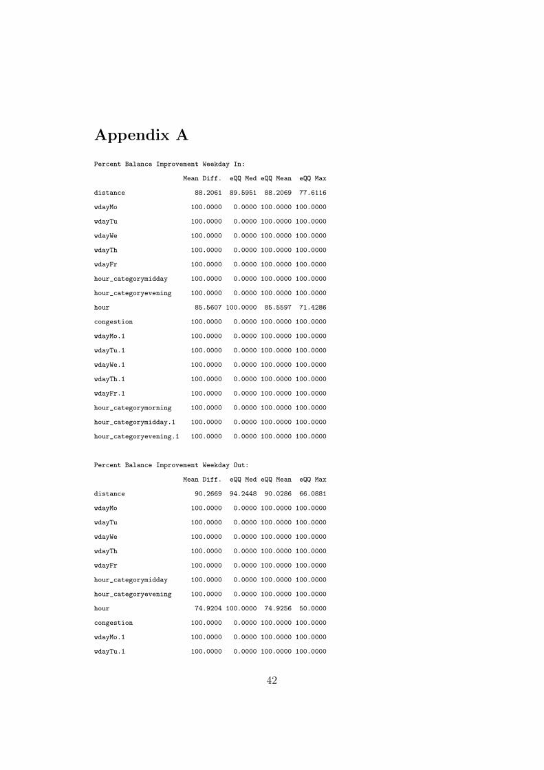
Appendix A
Percent Balance Improvement Weekday In:
Mean Diff. eQQ Med eQQ Mean eQQ Max
distance 88.2061 89.5951 88.2069 77.6116
wdayMo 100.0000 0.0000 100.0000 100.0000
wdayTu 100.0000 0.0000 100.0000 100.0000
wdayWe 100.0000 0.0000 100.0000 100.0000
wdayTh 100.0000 0.0000 100.0000 100.0000
wdayFr 100.0000 0.0000 100.0000 100.0000
hour_categorymidday 100.0000 0.0000 100.0000 100.0000
hour_categoryevening 100.0000 0.0000 100.0000 100.0000
hour 85.5607 100.0000 85.5597 71.4286
congestion 100.0000 0.0000 100.0000 100.0000
wdayMo.1 100.0000 0.0000 100.0000 100.0000
wdayTu.1 100.0000 0.0000 100.0000 100.0000
wdayWe.1 100.0000 0.0000 100.0000 100.0000
wdayTh.1 100.0000 0.0000 100.0000 100.0000
wdayFr.1 100.0000 0.0000 100.0000 100.0000
hour_categorymorning 100.0000 0.0000 100.0000 100.0000
hour_categorymidday.1 100.0000 0.0000 100.0000 100.0000
hour_categoryevening.1 100.0000 0.0000 100.0000 100.0000
Percent Balance Improvement Weekday Out:
Mean Diff. eQQ Med eQQ Mean eQQ Max
distance 90.2669 94.2448 90.0286 66.0881
wdayMo 100.0000 0.0000 100.0000 100.0000
wdayTu 100.0000 0.0000 100.0000 100.0000
wdayWe 100.0000 0.0000 100.0000 100.0000
wdayTh 100.0000 0.0000 100.0000 100.0000
wdayFr 100.0000 0.0000 100.0000 100.0000
hour_categorymidday 100.0000 0.0000 100.0000 100.0000
hour_categoryevening 100.0000 0.0000 100.0000 100.0000
hour 74.9204 100.0000 74.9256 50.0000
congestion 100.0000 0.0000 100.0000 100.0000
wdayMo.1 100.0000 0.0000 100.0000 100.0000
wdayTu.1 100.0000 0.0000 100.0000 100.0000
42

wdayWe.1 100.0000 0.0000 100.0000 100.0000
wdayTh.1 100.0000 0.0000 100.0000 100.0000
wdayFr.1 100.0000 0.0000 100.0000 100.0000
hour_categorymorning 100.0000 0.0000 100.0000 100.0000
hour_categorymidday.1 100.0000 0.0000 100.0000 100.0000
hour_categoryevening.1 100.0000 0.0000 100.0000 100.0000
Percent Balance Improvement Weekend In:
Mean Diff. eQQ Med eQQ Mean eQQ Max
distance 97.1691 100 97.1771 58.1291
wdaySo 100.0000 0 100.0000 100.0000
wdaySa 100.0000 0 100.0000 100.0000
hour 97.0831 100 97.5512 50.0000
congestion 100.0000 0 100.0000 100.0000
wdaySo.1 100.0000 0 100.0000 100.0000
wdaySa.1 100.0000 0 100.0000 100.0000
Percent Balance Improvement Weekend Out:
Mean Diff. eQQ Med eQQ Mean eQQ Max
distance 42.3380 66.8016 40.8860 49.9502
wdaySo 100.0000 0.0000 100.0000 100.0000
wdaySa 100.0000 0.0000 100.0000 100.0000
hour 16.1502 0.0000 15.5461 0.0000
congestion 100.0000 0.0000 100.0000 100.0000
wdaySo.1 100.0000 0.0000 100.0000 100.0000
wdaySa.1 100.0000 0.0000 100.0000 100.0000
43

Figure 7: Quanatile-Quantile Plot Weekday Matched Sample
−4 −2 0 2 4
20
40
60
Weekday In Wet
Theoretical Quantiles
Sa
mp
le Q
ua
ntile
s
−4 −2 0 2 4
10
20
30
40
50
60
Weekday In Dry
Theoretical Quantiles
Sa
mp
le Q
ua
ntile
s
−4 −2 0 2 4
20
40
60
80
Weekday Out Wet
Theoretical Quantiles
Sa
mp
le Q
ua
ntile
s
−4 −2 0 2 4
20
40
60
80
Weekday Out Dry
Theoretical Quantiles
Sa
mp
le Q
ua
ntile
s
44

Figure 8: Quanatile-Quantile Plot Weekend Matched Sample
−2 0 2
10
30
50
70
Weekend In Wet
Theoretical Quantiles
Sa
mp
le Q
ua
ntile
s
−2 0 2
20
30
40
50
60
Weekend In Dry
Theoretical Quantiles
Sa
mp
le Q
ua
ntile
s
−4 −2 0 2 4
20
40
60
80
Weekend Out Dry
Theoretical Quantiles
Sa
mp
le Q
ua
ntile
s
−4 −2 0 2 4
10
30
50
70
Weekend Out Wet
Theoretical Quantiles
Sa
mp
le Q
ua
ntile
s
45

Figure 9: Density Plot Weekday Matched Sample
Weekday In Dry
m.final_wday_in_momi$speed[m.final_wday_in_momi$category_n
Density
10 20 30 40 50 60
0.0
00.0
20.0
40.0
60.0
80.1
0
Weekday In Wet
m.final_wday_in_momi$speed[m.final_wday_in_momi$category_n
Density
20 30 40 50 60 70
0.0
00.0
20.0
40.0
60.0
80.1
0
Weekday Out Dry
Density
20 30 40 50 60 70 80
0.0
00.0
20.0
40.0
60.0
8
Weekday Out Wet
Density
20 40 60 80
0.0
00.0
20.0
40.0
60.0
8
46

Figure 10: Density Plot Weekend Matched Sample
Weekend In Dry
m.final_wend_in$speed[m.final_wend_in$category_numer
Density
20 30 40 50 60
0.0
00.0
20.0
40.0
60.0
8
Weekend In Wet
m.final_wend_in$speed[m.final_wend_in$category_numer
Density
10 20 30 40 50 60 70
0.0
00.0
20.0
40.0
60.0
80.1
0
Weekend Out Dry
Density
20 40 60 80 100
0.0
00.0
20.0
40.0
6
Weekend Out Wet
Density
10 20 30 40 50 60 70 80
0.0
00.0
20.0
40.0
60.0
8
47

References
Aarts, L., & Van Schagen, I. (2006). Driving speed and the risk of road
crashes: A review. Accident Analysis and Prevention, 38 (2), 215–224.
Almqvist, C., & Heinig, K. (2013). European accident research and safety
report 2013. Stockholm: Volvo.
Andrey, J., & Olley, R. (1990). The relationship between weather and road
safety: Past and future research directions. Climatological Bulletin, 24 (3),
123–127.
Andrey, J., & Yagar, S. (1993). A temporal analysis of rain-related crash
risk. Accident Analysis and Prevention, 25 (4), 465–472.
ASTRA. (2016). Unfallstatistik 2015 (Tech. Rep.). Bundesamt fur Strassen.
Bertness, J. (1980). Rain-related impacts on selected transportation activi-
ties and utility services in the chicago area. Journal of Applied Meteorology ,
19 (5), 545–556.
Billot, R., El Faouzi, N.-E., & De Vuyst, F. (2009). Multilevel assessment
of the impact of rain on drivers’ behavior: Standardized methodology and
empirical analysis. Transportation Research Record: Journal of the Trans-
portation Research Board(2107), 134–142.
BITRE. (2015). International road safety comparisons 2013. Bureau of
Infrastructure, Transport and Regional Economics (BITRE).
48

Brodsky, H., & Hakkert, A. S. (1988). Risk of a road accident in rainy
weather. Accident Analysis and Prevention, 20 (3), 161–176.
Chowdhury, D., Santen, L., & Schadschneider, A. (2000). Statistical physics
of vehicular traffic and some related systems. Physics Reports , 329 (4),
199–329.
Daganzo, C., & Daganzo, C. (1997). Fundamentals of transportation and
traffic operations (Vol. 30). Pergamon Oxford.
de Bellis, E., Schulte-Mecklenbeck, M., Brucks, W., Hermann, A., & Hertwig,
R. (2015, June). Blind haste: As light decreases, speeding increases.
Edwards, J. B. (1999). Speed adjustment of motorway commuter traffic to
inclement weather. Transportation Research Part F: Traffic Psychology
and Behaviour , 2 (1), 1–14.
Eisenberg, D. (2004). The mixed effects of precipitation on traffic crashes.
Accident analysis and prevention, 36 (4), 637–647.
El Faouzi, N.-E., Billot, R., Nurmi, P., & Nowotny, B. (2010). Effects
of adverse weather on traffic and safety: State-of-the-art and a european
initiative. In 15th international road weather conference.
Elvik, R. (2003). Assessing the validity of road safety evaluation studies
by analysing causal chains. Accident Analysis & Prevention, 35 (5),
741–748.
49

Elvik, R. (2004). To what extent can theory account for the findings of
road safety evaluation studies? Accident Analysis and Prevention, 36 (5),
841–849.
Evans, L. (1991). Traffic safety and the driver. Science Serving Society.
Fridstrøm, L., Ifver, J., Ingebrigtsen, S., Kulmala, R., & Thomsen, L. K.
(1995). Measuring the contribution of randomness, exposure, weather,
and daylight to the variation in road accident counts. Accident Analysis
and Prevention, 27 (1), 1–20.
Gao, H. O., & Niemeier, D. A. (2007). The impact of rush hour traffic and
mix on the ozone weekend effect in southern california. Transportation
Research Part D: Transport and Environment , 12 (2), 83–98.
Garber, N. J., & Gadirau, R. (1988). Speed variance and its influence on
accidents. AAA Foundation for Traffic Safety .
Google. (2016, August). Google maps screenshot fruttalstrasse. Retrieved
18.08.2016, from https://goo.gl/maps/1UEDd5HMXc32
Haddon, W. (1972). A logical framework for categorizing highway safety
phenomena and activity. Journal of Trauma and Acute Care Surgery ,
12 (3), 193–207.
Haight, F. A. (1986). Risk, especially risk of traffic accident. Accident
Analysis and Prevention, 18 (5), 359–366.
Hamilton, B.-A. (2012). Ten-year averages from 2002 to 2012
based on nhtsa data (Tech. Rep.). US Department of Transporta-
50

tion - Federal Highway Administration. Retrieved 03.08.2016, from
http://www.ops.fhwa.dot.gov/weather/
Hauer, E. (2002). Fishing for safety information in the murky waters of re-
search reports. In Transportation Research Board annual meeting, Wash-
ington DC.
Jagerbrand, A. K., & Sjobergh, J. (2016). Effects of weather conditions,
light conditions, and road lighting on vehicle speed. SpringerPlus , 5 (1),
1–17.
Liang, W., Kyte, M., Kitchener, F., & Shannon, P. (1998). Effect of envi-
ronmental factors on driver speed: A case study. Transportation Research
Record: Journal of the Transportation Research Board(1635), 155–161.
Padget, E., Knapp, K., & Thomas, G. (2001). Investigation of winter-weather
speed variability in sport utility vehicles, pickup trucks, and passenger cars.
Transportation Research Record: Journal of the Transportation Research
Board(1779), 116–124.
Sabey, B., & Staughton, G. (1975). Interacting roles of road environment
vehicle and road user in accidents. Ceste I Mostovi .
Schuster, A., Sattler, J., & Hoffman, S. (2011). Bestimmen der
aktuellen Abmessungen differenzierter Personen- Bemessungsfahrzeuge
(Tech. Rep.). Westsachsische Hochschule Zwickau.
Shermer, M. (2008). Folk numeracy and middle land. Scientific American,
299 (3), 40–40.
51

Sherretz, L. A., & Farhar, B. C. (1978). An analysis of the relationship
between rainfall and the occurrence of traffic accidents. Journal of Applied
Meteorology , 17 (5), 711–715.
Siegel, S. (1956). Nonparametric statistics for the behavioral sciences.
McGraw-Hill .
Thadewald, T., & Buning, H. (2007). Jarque–Bera test and its competitors
for testing normality: A power comparison. Journal of Applied Statistics ,
34 (1), 87–105.
Tiwari, G., Mohan, D., & Muhlrad, N. (2005). The way forward: Trans-
portation planning and road safety. Delhi: McMillan India Ltd .
Treiber, M., & Kesting, A. (2010). Darstellung von Querschnittsdaten. In
Verkehrsdynamik und-simulation (pp. 25–36). Springer.
Unrau, D., & Andrey, J. (2006). Driver response to rainfall on urban ex-
pressways. Transportation Research Record: Journal of the Transportation
Research Board(1980), 24–30.
Wilde, G. (1976). The risk compensation theory of accident causation and
its practical consequences for accident prevention. Transportation Research
Record: Journal of the Transportation Research Board .
Wilde, G. (1988). Risk homeostasis theory and traffic accidents: propositions,
deductions and discussion of dissension in recent reactions. Ergonomics ,
31 (4), 441–468.
52

Wu, M.-C., Lee, L.-C., & Shih, M.-C. (1998). Neuro-fuzzy controller design
of the anti-lock braking system. JSME International Journal Series C
Mechanical Systems, Machine Elements and Manufacturing , 41 (4), 836–
843.
53

List of Tables
1 Haddon Matrix . . . . . . . . . . . . . . . . . . . . . . . . . . 9
2 Speed Statistics – Entire Sample . . . . . . . . . . . . . . . . . 21
3 Variables of Interest . . . . . . . . . . . . . . . . . . . . . . . 26
4 Sample Size Matching . . . . . . . . . . . . . . . . . . . . . . 27
5 Weekday Morning and Evening Differences . . . . . . . . . . . 28
6 Summary and Results Wilcoxon Signed Rank Test with Con-
tinuity Correction . . . . . . . . . . . . . . . . . . . . . . . . . 30
7 Fligner-Killeen Test of Homogeneity of Variances . . . . . . . 31
8 Braking Distances . . . . . . . . . . . . . . . . . . . . . . . . . 32
9 Causal Chain Model – Effects of Wet Pavement . . . . . . . . 38
10 Research Design . . . . . . . . . . . . . . . . . . . . . . . . . . 40
List of Figures
1 Causal Chain Model . . . . . . . . . . . . . . . . . . . . . . . 10
2 Study Site Map . . . . . . . . . . . . . . . . . . . . . . . . . . 20
3 Study Site Streetview . . . . . . . . . . . . . . . . . . . . . . . 21
4 Traffic Counts . . . . . . . . . . . . . . . . . . . . . . . . . . . 22
5 Speed Counts . . . . . . . . . . . . . . . . . . . . . . . . . . . 22
6 Balanced Sample Speed Plot . . . . . . . . . . . . . . . . . . . 28
7 Quanatile-Quantile Plot Weekday Matched Sample . . . . . . 44
8 Quanatile-Quantile Plot Weekend Matched Sample . . . . . . 45
9 Density Plot Weekday Matched Sample . . . . . . . . . . . . . 46
54

10 Density Plot Weekend Matched Sample . . . . . . . . . . . . . 47
55

Statement of Authorship
I hereby declare that I have written this thesis without any help from others
and without the use of documents and aids other than those stated above.
I have mentioned all used sources and cited them correctly according to
established academic citation rules. I am aware that otherwise the Senat is
entitled to revoke the degree awarded on the basis of this thesis, according
to article 36 paragraph 1 letter o of the University Act from 5 September
1996.
Berne, September 13, 2016
Ozan Harman
56