Road lighting Foreword - nmfv.dk · road lighting and provided recommendations for the lighting levels to use on different roads. The attitude is that the experts are the only ones

Road lighting

Kai Sørensen, 8 April 2013

Foreword

This textbook on road lighting has been prepared by the NMF with the scope to collect the knowledge that

has been obtained in a number of projects carried out by the NMF or with the assistance of members of the

NMF, to put this knowledge into an international and practical perspective, and make it available for future

use, in particular for the education of persons working in the field of road signing.

It is the intention that the textbook itself is translated to Nordic language, when this is relevant, while the

annexes A to C with more detailed information remain in the English language only. It may also be useful to

translate the annex X on light and units.

Similar textbooks on road markings and road surfaces and retroreflective road equipment have already been

prepared. It is a further intention to prepare additional textbooks on other types of road equipment on which

the NMF has worked; including variable message signs, signal heads and yellow flashing lights at road

works.

NMF (Nordisk Møde for Forbedret vejudstyr – translates to Nordic Meeting for improved road equipment)

was founded in 1973 and is a well established forum in the Nordic countries for co-operation between the

national road administrations and researchers in the field of development and improvement of road

equipment. It is the scope of the NMF to provide – through FoU activities – the knowledge basis for

improvement of the visibility and/or legibility of the road and its various components (road markings, road

signs, road lighting, retroreflectors, delineators, signal and warning lights etc.).

The road users orientation and understanding of the road and current traffic situations is to be supported

through improvement of the transfer of information between the road and the road user.

An important activity of the NMF is to take part in the European standards work within the CEN. Through

the conduction of research, whose results should have directs consequences for the drafting of standards for

road equipment, the Nordic countries together have the possibility of playing a positive and decisive role in

this work.

2

Contents page

Introduction 3

1. History of modern road lighting 5

2. A basis for the selection of lighting classes 9

2.1 Introduction 9

2.2 Lighting classes of EN 13201-2 9

2.3 The visual performance offered by road lighting levels 10

2.4 Disability glare and its influence on visual performance 11

2.5 Considerations for the selection of lighting classes 13

3. Performance requirements for road lighting 15

3.1 The M, C, P and HS lighting classes 15

3.2 Average maintained value and uniformity 17

3.3 Additional requirements for the M classes 18

4. Light sources for road lighting 21

4.1 Introduction and summary 21

4.2 Visible light 23

4.3 Colour of emitted light 26

4.4 Correlated colour temperature 27

4.5 Colour rendering index 28

4.6 Production of light 28

4.7 Light sources 33

6. Luminaires for road lighting 39


6.2 Optics for luminaires 40

6.3 Light distributions of luminaires 44

6.4 Luminous intensity classes 52

6.5 Glare index classes 54

7. Lighting installations 55


7.2 Description of lighting installations 55

7.3 National requirements for road lighting installations 58

7.4 Lighting efficiency of road lighting installations 59

Literature 61

Annex A: Performance characteristics for road lighting 63

Annex B: Light sources for road lighting 105

Annex C: Luminaires for road lighting 137

Annex X: Lighting concepts and units used for road equipment 161

3

Introduction

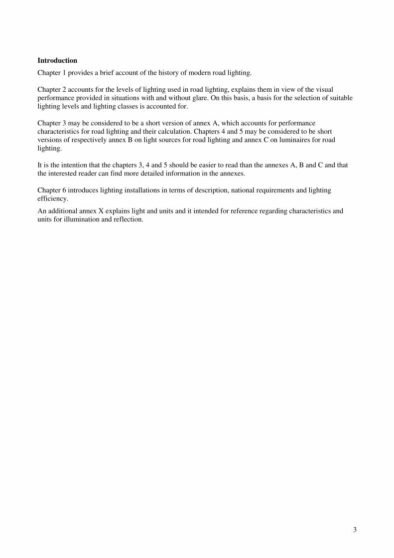
Chapter 1 provides a brief account of the history of modern road lighting.

Chapter 2 accounts for the levels of lighting used in road lighting, explains them in view of the visual

performance provided in situations with and without glare. On this basis, a basis for the selection of suitable

lighting levels and lighting classes is accounted for.

Chapter 3 may be considered to be a short version of annex A, which accounts for performance

characteristics for road lighting and their calculation. Chapters 4 and 5 may be considered to be short

versions of respectively annex B on light sources for road lighting and annex C on luminaires for road

lighting.

It is the intention that the chapters 3, 4 and 5 should be easier to read than the annexes A, B and C and that

the interested reader can find more detailed information in the annexes.

Chapter 6 introduces lighting installations in terms of description, national requirements and lighting

efficiency.

An additional annex X explains light and units and it intended for reference regarding characteristics and

units for illumination and reflection.

4

5

1. History of modern road lighting

Electrical road lighting started with the incandescent lamp and was developed in steps with each invention

and improvement of more efficient light sources in the sequence of low-pressure sodium lamps, mercury

lamps, fluorescent tubes, high pressure sodium lamps, compact fluorescent lamps and metal halide lamps.

The development of reflector optics has been linked to the these steps. It started with parabolic optics for the

mercury lamp, allowed by its relatively small and compact shape, and continued with pot optics for the

tubular high pressure sodium lamps and metal halide lamps allowed by their even smaller luminous shapes.

The driving force behind these steps of development has been the economy of road lighting. This is clearly

demonstrated by the wide spread use of high pressure sodium lamp in spite of its poor quality of light in

terms of colour of light and colour rendition.

The latest step is the LED module, that integrates the LED light sources with optics and electrical supply and

control gear. The LED module can match the lighting economy of the high pressure sodium lamp and may

pass it in the near future, and simultaneous provide light of a higher quality.

Early methods for designing road lighting installations were recipe methods for the spacing of luminaires or

the luminous output required per square metre of the illuminated area. The reflector optics lead to more

detailed design methods involving the distribution of illuminance or luminance of the illuminated area.

These design methods were developed in the CIE (Commission Internationale d’Eclairage) by a relatively

small group of experts representing lighting companies, road administrations and institutes. With a start

probably in mid 1960’s the methods were fully developed during the 1970’s when photometry of light

sources and luminaires - and computer calculations - had gradually become available. The CIE published

several reports and recommendations on road lighting in this period, later to become revised and

supplemented with more reports during the years.

The CIE is still active in this field, and still with a relatively small group of experts in CIE division 4. There

has of course been a gradual change of the experts over such a long period, but with a long average

membership and a continuation of the original pioneering spirit.

The CIE has some affiliation to ISO (International Standards Organisation), but no direct recognition of

governments. Nevertheless, the CIE publications have been important for the development of national road

lighting standards as they were the only international publications available.

The group of experts invented not only the complex design methods, but also the quality characteristics for

road lighting and provided recommendations for the lighting levels to use on different roads. The attitude is

that the experts are the only ones with a knowledge and have the responsibility for recommending good road

lighting and traffic safety all over the world.

Nevertheless, when the EN 13201 series of European standards was drafted during the 1990’s – to some

degree by the same experts - it turned out that the more or less common basis in CIE publications had

resulted in different interpretations in national road lighting standards. This was a surprise to the experts but

they had eventually to accept that the EN 13201 series provide some freedom in view of national traditions.

It was harder for the experts to accept that a part 1 on the selection of lighting classes was not welcome – it

eventually became a technical report of an informative nature. Because of disputes over this, the EN 13201

series was not published until 2003.

6

The two essential parts of the EN 13201 series are EN 13201-2 “Road lighting — Part 2: Performance

requirements” which defines lighting classes for different applications and EN 13201-3 “Road lighting —

Part 3: Calculation of performance” which defines methods of design calculations.

There is an EN 13201-4 “Road lighting — Part 4: Methods of measuring lighting performance”, but it should

be realized that road lighting installations are “works” in the sense of the Construction Products Regulation.

As with other works (buildings, bridges etc.), the performance is provided by design, quality assurance of the

products installed in the works (in this case lighting columns, luminaires, light sources etc.) and of the work

itself. Measurements are rarely carried out except in simplified manners as they are difficult and expensive,

involve closing of roads, and do not place the responsibility for deviations. Measurement of performance is

not considered further in this textbook.

A revision of the EN 13201 series was initiated in 2008. The group of experts had armed itself with a draft

revision of CIE 115 “Lighting of roads for motor and pedestrian traffic” and was ready to fight for a higher

status of part 1 and “harmonisation” of road lighting in Europe.

Now, about 5 years later (Spring 2013) the final drafts show an unchanged status of Part 1 and the same

degree of freedom in view of national traditions. But of course there is some improvement of the technical

contents. The revision includes addition of an EN 13201-5 “Road lighting – Part 5: Energy performance in

road lighting”. The addition of this part is only partly successful, as the final draft is of poor quality.

In the following it is assumed that above-mentioned final drafts are accepted in approximately the form there

are in at present.

The group of experts is not infallible. CIE 23 on international recommendations for motorway lighting from

1973 pointed to much too high lighting levels. The recommendations were followed in a period until the

practical lighting world gradually reduced the levels to about half.

Claims are often made of the role of road lighting for traffic safety, but these are generally unsubstantiated.

Some studies do indicate accident reductions by improved road lighting, but other studies are inconclusive or

point the other way. A real proof that road lighting levels are important for traffic safety has not been

provided. There is no basis at all for claims regarding less important lighting characteristics such as

uniformities of lighting.

The problem is that a good study has to involve large numbers of roads with control of all variables over a

period of years. It is almost impossible to do such a study in the practical world.

It should be stated that road lighting is of course important. If the road lighting is turned off in a city area, the

traffic comes to a standstill and accidents occur. If the road lighting is turned off in a domestic area, some

residents will stay at home after dark and many will object. The question is how much lighting is needed to

serve the purpose. Practical experience and common sense is as important as expertise. The final choice of

lighting level will involve a compromise between the needs of road users and the cost of road lighting.

Traffic accident rates have been steadily decreasing in many countries, and probably at a higher rate at night

on roads with road lighting. This cannot readily be assigned to road lighting as other factors are important.

Such may be shifting of a substantial traffic volume from ordinary traffic routes to the much safer

motorways, introduction of clear distinctions between traffic routes and domestic roads, improvement of

road geometries and use of more and better road equipment. An additional factor is the improvement of the

passive safety of the cars themselves.

The group of experts has shown too little respect for complications as shown by the introduction of concepts

like the luminance design, Threshold Increment and facial recognition:

7

- Luminance design is complex by involving the reflection properties of the road surfaces and the

locations of drivers on the road. It is a question if the gain outweighs the disadvantage of the

complexity.

- TI (Threshold Increment) as a measure of disability glare from the lighting installation is almost

incomprehensible – it is the percentage increase in the contrast of objects needed to make them as

visible as they would have been in the absence of glare. That is nonsense, and does not tell how to cope

with the glare.

- Facial recognition – to make the lighting sufficient to allow that one person is able to recognize a person

he meets on the road from some distance – is impractical and almost impossible to achieve on a

reasonable economical basis. It is described by semi-cylindrical lighting, which has the preferred

direction of the semi-cylinder representing the face of the person and therefore needs to be evaluated for

different directions of the face. Further, it takes much lighting into the face of a person to make him

recognizable at a distance, which is expensive and might prevent his recognition of the other person

because of glare. Nevertheless, this concept took up much attention in the CIE in a period and survives

as the supplementary SC lighting classes in EN 13201-2.

The concept of hemispherical illuminance is, on the other hand, simple and practical. It places equal weight

to all inclinations of surfaces and provides probably a better description of the lighting needs of pedestrians

and cyclists than the horizontal illuminance. In any case, it has the practical aspect of allowing lower

mountings of the luminaires than the horizontal illuminance – so that lighting poles can be kept low at areas

lighted for the benefit of pedestrians. This concept did not get much attention, but it is included in the HS

classes of EN 13201-2.

The author of this book was one of the experts for a long period and should feel some guilt. However, a

couple of matters provide consolation:

- The whole construction does work in practise. The necessary data are available, the design calculations

are strictly standardised and software is available as freeware.

- There is some sense in luminance design as a road of uniform appearance does not steal attention from

the main visual tasks.

- The difference between illuminance and luminance design is relatively small, when designing for a wet

condition in addition to the dry condition. This is done in the Nordic countries.

- The concept of facial recognition is probably used rarely. if at all.

- The concept of hemispherical illuminance is available for use in a few countries (perhaps only

Denmark).

8

9

2. A basis for the selection of lighting classes

2.1 Introduction

The basis for the selection of lighting classes is introduced in 2.5 after these introductory clauses:

- 2.2 lighting classes of EN 13201-2

- 2.3 the visual performance offered by road lighting levels

- 2.4 disability glare and its influence on visual performance.

2.2 Lighting classes of EN 13201-2

EN 13201-2 “Road lighting — Part 2: Performance requirements” defines the M, C, P and HS series of

lighting classes that are introduced in table 1.

Table 1: Steps of road lighting levels.

Road users

Lighting for drivers of motorized vehicles Lighting for pedestrians and cyclists

Type of road area

Traffic routes of medium to high driving speeds

Conflict areas such as shopping streets, road intersections of some complexity, round-abouts, queuing areas etc.

Footways, cycleways, emergency lanes and other road areas lying separately or along the carriageway of a traffic route, and for residential roads, pedestrian streets, parking places, schoolyards etc.

Lighting level

M classes

L in cd/m2

[minimum maintained]

C classes

E in lx [minimum maintained]

P classes

E in lx a


HS classes

E hs in lx [minimum maintained]

1 C0 50

2 M1 2,00 C1 30

3 M2 1,50 C2 20,0

4 M3 1,00 C3 15,0 P1 15,0

5 M4 0,75 C4 10,0 P2 10,0

6 M5 0,50 C5 7,50 P3 7,50 HS1 5,00

7 M6 0,30 P4 5,00 HS2 2,50

8 P5 3,00

9 P6 2,00 HS3 1,00

10 P7 performance

not determined

HS4 performance not determined

The M classes are intended for drivers of motorised vehicles on traffic routes of medium to high driving

speeds. The C classes are primarily intended also for drivers of motorised vehicles, but on conflict areas such

as road intersections of some complexity, roundabouts, queuing areas etc.

10

The P classes and the HS classes are alternatives to each other and intended for pedestrians and pedal cyclists

on footways, cycleways, emergency lanes and other road areas lying separately or along the carriageway of a

traffic route, and for residential roads, pedestrian streets, parking places, schoolyards etc.

NOTE: EN 13201-2 also defines SC and EV classes for additional requirements. The SC classes are intended as an

additional class for pedestrian areas for the purposes of reducing crime and increasing feelings of safety. The EV classes

are intended as an additional class in situations where vertical surfaces need to be seen, e.g. interchange areas. These

classes are not considered in this textbook.

2.3 The visual performance offered by road lighting levels

The lighting levels of the lighting classes of table 1 interlock approximately in such a manner that they can

be arranged into a total of 10 steps as also indicated in table 1.

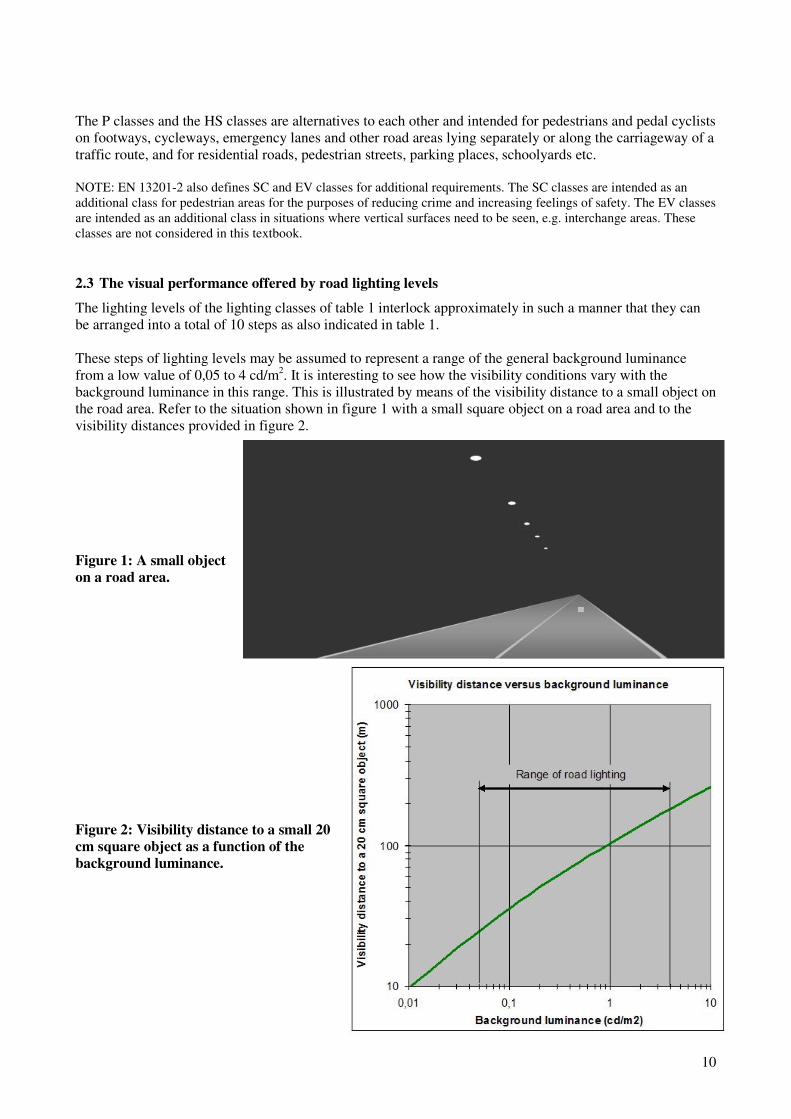
These steps of lighting levels may be assumed to represent a range of the general background luminance

from a low value of 0,05 to 4 cd/m2. It is interesting to see how the visibility conditions vary with the

background luminance in this range. This is illustrated by means of the visibility distance to a small object on

the road area. Refer to the situation shown in figure 1 with a small square object on a road area and to the

visibility distances provided in figure 2.

Figure 1: A small object

on a road area.

Figure 2: Visibility distance to a small 20

cm square object as a function of the

background luminance.

11

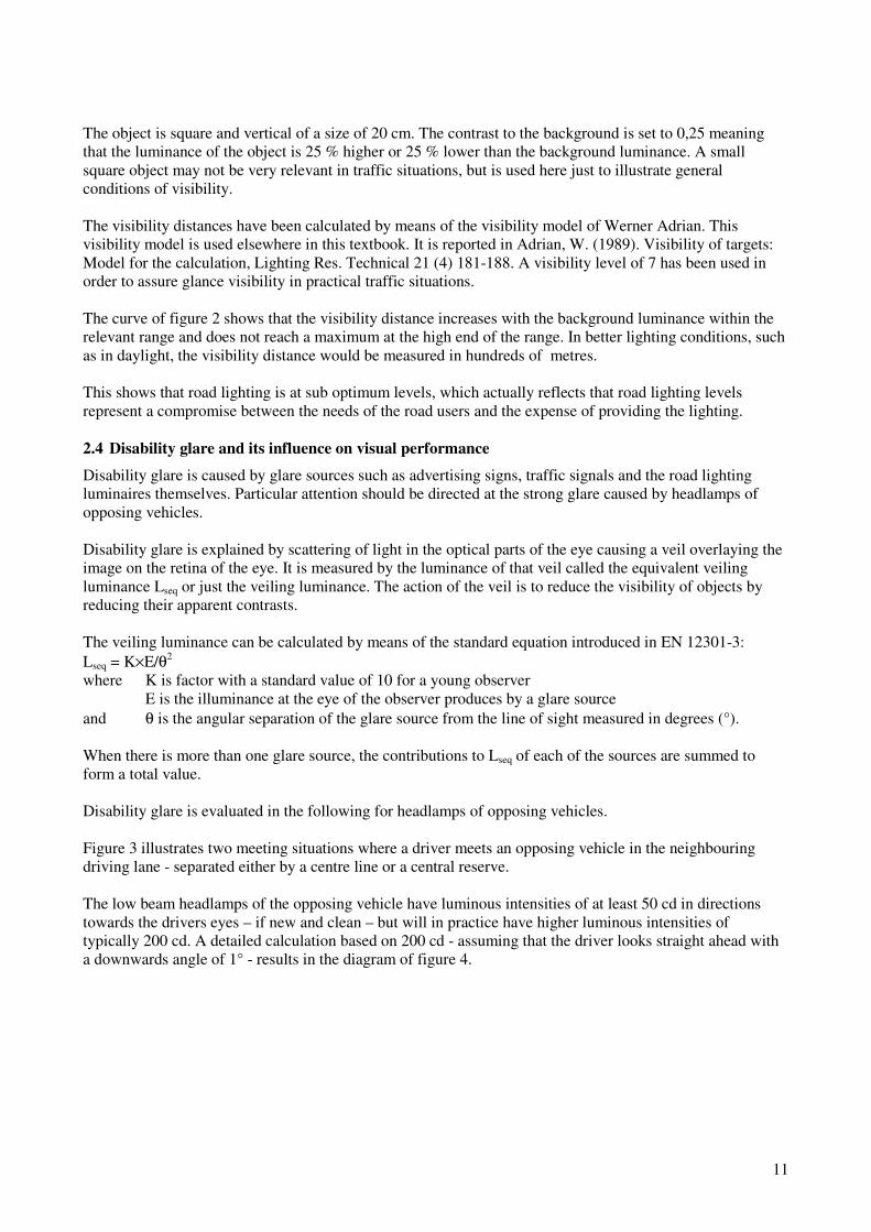
The object is square and vertical of a size of 20 cm. The contrast to the background is set to 0,25 meaning

that the luminance of the object is 25 % higher or 25 % lower than the background luminance. A small

square object may not be very relevant in traffic situations, but is used here just to illustrate general

conditions of visibility.

The visibility distances have been calculated by means of the visibility model of Werner Adrian. This

visibility model is used elsewhere in this textbook. It is reported in Adrian, W. (1989). Visibility of targets:

Model for the calculation, Lighting Res. Technical 21 (4) 181-188. A visibility level of 7 has been used in

order to assure glance visibility in practical traffic situations.

The curve of figure 2 shows that the visibility distance increases with the background luminance within the

relevant range and does not reach a maximum at the high end of the range. In better lighting conditions, such

as in daylight, the visibility distance would be measured in hundreds of metres.

This shows that road lighting is at sub optimum levels, which actually reflects that road lighting levels

represent a compromise between the needs of the road users and the expense of providing the lighting.

2.4 Disability glare and its influence on visual performance

Disability glare is caused by glare sources such as advertising signs, traffic signals and the road lighting

luminaires themselves. Particular attention should be directed at the strong glare caused by headlamps of

opposing vehicles.

Disability glare is explained by scattering of light in the optical parts of the eye causing a veil overlaying the

image on the retina of the eye. It is measured by the luminance of that veil called the equivalent veiling

luminance Lseq or just the veiling luminance. The action of the veil is to reduce the visibility of objects by

reducing their apparent contrasts.

The veiling luminance can be calculated by means of the standard equation introduced in EN 12301-3:

Lseq = K×E/θ2

where K is factor with a standard value of 10 for a young observer

E is the illuminance at the eye of the observer produces by a glare source

and θ is the angular separation of the glare source from the line of sight measured in degrees (°).

When there is more than one glare source, the contributions to Lseq of each of the sources are summed to

form a total value.

Disability glare is evaluated in the following for headlamps of opposing vehicles.

Figure 3 illustrates two meeting situations where a driver meets an opposing vehicle in the neighbouring

driving lane - separated either by a centre line or a central reserve.

The low beam headlamps of the opposing vehicle have luminous intensities of at least 50 cd in directions

towards the drivers eyes – if new and clean – but will in practice have higher luminous intensities of

typically 200 cd. A detailed calculation based on 200 cd - assuming that the driver looks straight ahead with

a downwards angle of 1° - results in the diagram of figure 4.

12

A: without central reserve.

B: with a central reserve.

Figure 3: Meeting situations without (A) and with a central reserve (B).

Figure 4: Veiling luminance in meeting

situations.

The veiling luminance is seen to be quite high for the situation without central reserve and much lower for

the situation with a central reserve. It increases as the two vehicles approach each other until shortly before

they pass by each other. It will then drop-off quickly, but this feature is not shown in the diagram of figure 4.

If the driver faces two or more opposing vehicles as illustrated in figure 5, the total veiling luminance may

easily become for instance 0,25 cd/m2 or higher.

Figure 5: Meeting situation with two

opposing vehicles.

Veiling luminance in meeting situations

0,00

0,02

0,04

0,06

0,08

0,10

0,12

0,14

20 70 120 170

Distance between vehicles (m)

Veilin

g lu

min

an

ce (

cd

/m2)

Without central reserve

With central reserve of 3 m

13

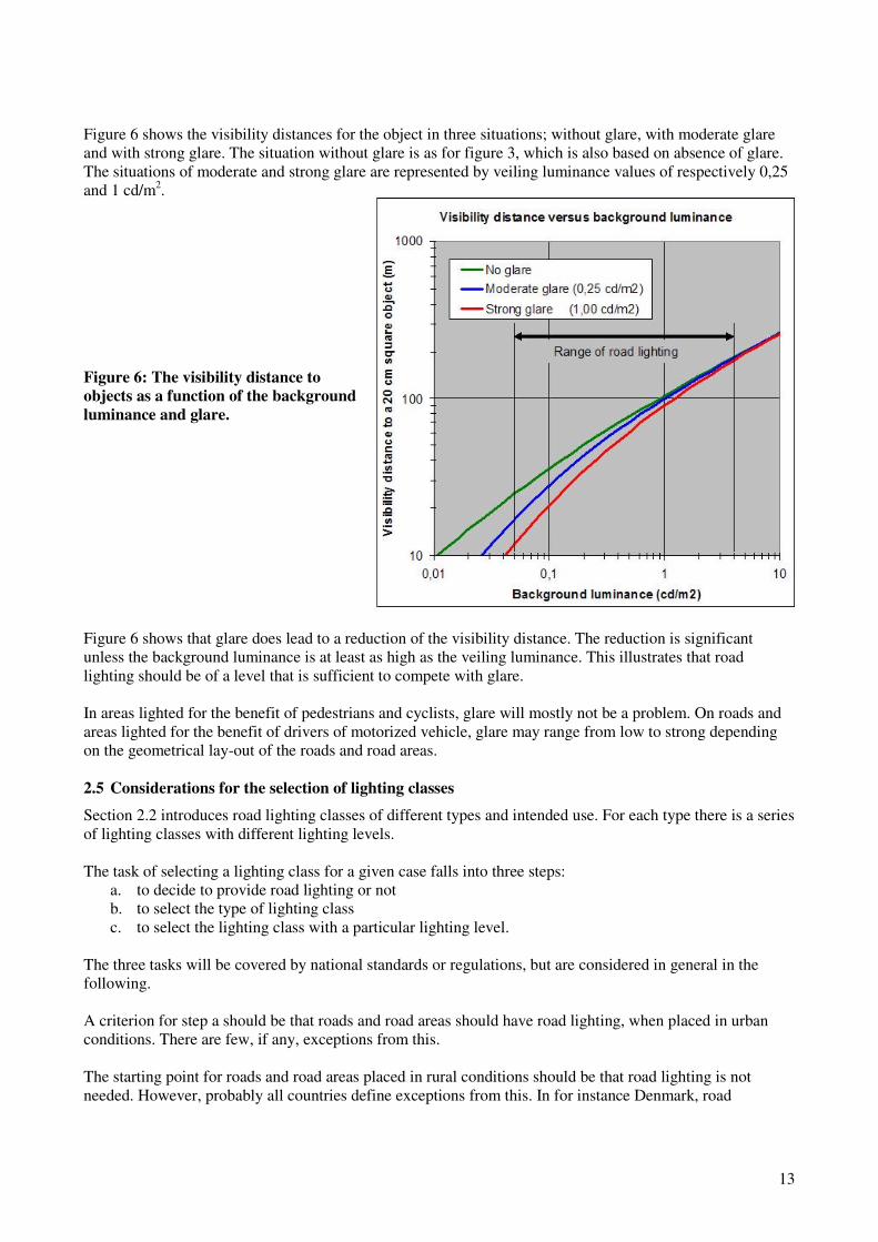
Figure 6 shows the visibility distances for the object in three situations; without glare, with moderate glare

and with strong glare. The situation without glare is as for figure 3, which is also based on absence of glare.

The situations of moderate and strong glare are represented by veiling luminance values of respectively 0,25

and 1 cd/m2.

Figure 6: The visibility distance to

objects as a function of the background

luminance and glare.

Figure 6 shows that glare does lead to a reduction of the visibility distance. The reduction is significant

unless the background luminance is at least as high as the veiling luminance. This illustrates that road

lighting should be of a level that is sufficient to compete with glare.

In areas lighted for the benefit of pedestrians and cyclists, glare will mostly not be a problem. On roads and

areas lighted for the benefit of drivers of motorized vehicle, glare may range from low to strong depending

on the geometrical lay-out of the roads and road areas.

2.5 Considerations for the selection of lighting classes

Section 2.2 introduces road lighting classes of different types and intended use. For each type there is a series

of lighting classes with different lighting levels.

The task of selecting a lighting class for a given case falls into three steps:

a. to decide to provide road lighting or not

b. to select the type of lighting class

c. to select the lighting class with a particular lighting level.

The three tasks will be covered by national standards or regulations, but are considered in general in the

following.

A criterion for step a should be that roads and road areas should have road lighting, when placed in urban

conditions. There are few, if any, exceptions from this.

The starting point for roads and road areas placed in rural conditions should be that road lighting is not

needed. However, probably all countries define exceptions from this. In for instance Denmark, road

14

crossings with traffic signals, roundabouts and speed humps are illuminated. In some Nordic countries, some

roads in rural conditions are illuminated as a traffic safety measure.

The step b should normally not cause much difficulty, so it is mainly step c – selection of the lighting level -

that needs to be considered.

It should be stated first of all that roads should not be considered individually, but in connection with an

overall plan for road lighting in a larger area in general. The overall plan may include the type of road, the

character of the road lighting, the types of lighting classes, the levels lighting, use of dimming etc.

In 2.3 it is concluded that road lighting is at sub optimum levels, which actually reflects that road lighting

levels represent a compromise between the visual needs of the road users and the expense of providing the

lighting.

The choice of level should therefore reflect the visual needs of the road users. This introduces the following

considerations:

i. drivers of motorised vehicles need a higher lighting level than pedestrians and cyclists as they

need to see objects at a longer distance

ii. a higher driving speed should point towards a higher lighting level.

A higher lighting level leads not only to longer visibility distances, but also a faster visual scanning of a

complex scenery. This introduces additional considerations:

iii. road crossings and roundabouts should be illuminated to at least the highest level of road

lighting on adjacent roads

iv. the complexity of the road area as for instance measured by the number of driving lanes should

point towards a higher lighting level

v. the complexity of the traffic measured for instance by the presence of pedal cyclists or

occasional pedestrians on the carriageway should point towards a higher lighting level

In 2.4 it is concluded that the lighting level should be at least as high as the level of glare measured by the

veiling luminance. Glare by the headlamps of opposing cars is a particular problem. The general rule is

probably that road lighting should be able to compete with the general level of ambient light in the

surroundings. This introduces further considerations:

vi. opposing traffic without separation by a central reserve should point towards a higher lighting

level

vii. the level of road lighting should be at least the general level of ambient light in the surroundings

Disability glare from the luminaires of the lighting installations is discussed in A.9. It is concluded that this

glare can be significant even when the Threshold Increment is within the maximum values specified for the

M classes. This introduces one more consideration:

viii. it should point towards a lower lighting level when the glare from the luminaires of the lighting

installation is reduced by for instance use of luminaires of full cut-off (classes G*5 and G*6 in

particular, refer to 6.4)

The feeling of safety and the amenity of the lighting are other considerations for the lighting for pedestrians

at for instance shopping streets.

National specifications for the selection of lighting classes should include all these considerations in a

comparatively simple manner.

15

3. Performance requirements for road lighting

3.1 The M, C, P and HS lighting classes

The performance requirements for road lighting are those of the M, C, P and HS lighting classes of EN

13201-2 “Road lighting — Part 2: Performance requirements”. These are defined in tables 1, 2, 3 and 4

respectively of EN 13201-2. The contents of those tables are presented below in tables 2, 3, 4 and 5 for

convenience.


speeds. The lighting criteria are based on the luminance of the road surface of the carriageway. This involves

not only the reflection properties of the road surface, but also the location and the direction of sight of an

observer representing a driver.

The C classes are also intended for drivers of motorised vehicles, but for use on conflict areas such as

shopping streets, road intersections of some complexity, roundabouts and queuing areas, where the

conventions for road surface luminance calculations do not apply or are impracticable. Instead, the lighting

criteria are based on the horizontal illuminance on the carriageway. The lighting installations mostly

comprise poles at strategic places, each with one or more luminaires – often mounted with different

orientations.

The P and HS classes are intended for pedestrians and pedal cyclists on footways, cycleways, emergency

lanes and other road areas lying separately or along the carriageway of a traffic route, and for residential

roads, pedestrian streets, parking places, schoolyards etc.

Road areas along the carriageway of traffic routes or conflict areas are mostly illuminated by the lighting

installation that is intended primarily for the carriageway, but receive in some cases illumination by

additional luminaires. Road areas lying separately have their own lighting installations.

The lighting criteria of the P and HS classes are based on respectively the horizontal illuminance and the

hemispherical illuminance on the traffic area.

16

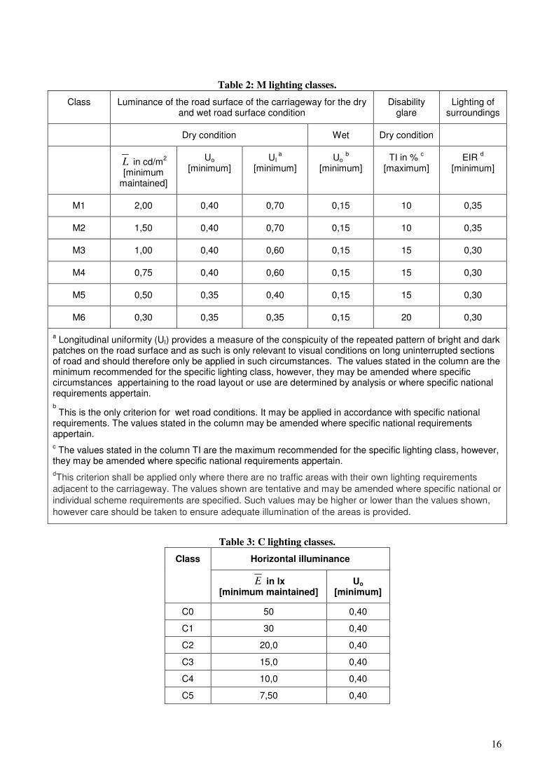
Table 2: M lighting classes.

Class Luminance of the road surface of the carriageway for the dry and wet road surface condition

Disability glare

Lighting of surroundings

Dry condition Wet Dry condition

L in cd/m2


Uo [minimum]

UI a

[minimum] Uo

b

[minimum] TI in %

c

[maximum] EIR

d

[minimum]

M1 2,00 0,40 0,70 0,15 10 0,35

M2 1,50 0,40 0,70 0,15 10 0,35

M3 1,00 0,40 0,60 0,15 15 0,30

M4 0,75 0,40 0,60 0,15 15 0,30

M5 0,50 0,35 0,40 0,15 15 0,30

M6 0,30 0,35 0,35 0,15 20 0,30

a Longitudinal uniformity (UI) provides a measure of the conspicuity of the repeated pattern of bright and dark

patches on the road surface and as such is only relevant to visual conditions on long uninterrupted sections of road and should therefore only be applied in such circumstances. The values stated in the column are the minimum recommended for the specific lighting class, however, they may be amended where specific circumstances appertaining to the road layout or use are determined by analysis or where specific national requirements appertain.

b

This is the only criterion for wet road conditions. It may be applied in accordance with specific national requirements. The values stated in the column may be amended where specific national requirements appertain.

c The values stated in the column TI are the maximum recommended for the specific lighting class, however,

they may be amended where specific national requirements appertain.

dThis criterion shall be applied only where there are no traffic areas with their own lighting requirements

adjacent to the carriageway. The values shown are tentative and may be amended where specific national or

individual scheme requirements are specified. Such values may be higher or lower than the values shown,

however care should be taken to ensure adequate illumination of the areas is provided.

Table 3: C lighting classes.

Class Horizontal illuminance


Uo [minimum]

C0 50 0,40

C1 30 0,40

C2 20,0 0,40

C3 15,0 0,40

C4 10,0 0,40

C5 7,50 0,40

17

Table 4: P lighting classes.


E in lx a

[minimum maintained] Emin in lx

[maintained]

P1 15,0 3,00

P2 10,0 2,00

P3 7,50 1,50

P4 5,00 1,00

P5 3,00 0,60

P6 2,00 0,40

P7 performance not determined performance not determined

a To provide for uniformity, the actual value of the maintained average

illuminance must not exceed 1,5 times the minimum E value indicated for the class.

Table 5: HS lighting classes.

Class Hemispherical illuminance


U0 minimum]

HS1 5,00 0,15

HS2 2,50 0,15

HS3 1,00 0,15

HS4 performance not determined performance not determined

3.2 Average maintained value and uniformity

The main requirement of a lighting class is the lighting level presented as a minimum requirement for the

maintained average value of the lighting parameter over the relevant road area. The lighting parameter for

the M classes is the road surface luminance, for the C and P classes it is the horizontal illuminance and for

the HS classes the hemispherical illuminance.

An average value is the simple average of values at locations covering the road area. The maintained average

value is in practice the nominal average value as determined for a new and clean lighting installation

multiplied by a maintenance factor with a value that takes gradual depreciation of the light output and

restoration of the light output at intervals into account.

Additional minimum requirements address the uniformity of the lighting parameter over the road area.

For the M, C and HS classes the uniformity is expressed by the overall uniformity defined as the ratio

between the lowest value at any location and the average value. The possible range of the overall uniformity

is from 0 to 1, where 0 means that parts of the road area receive no light at all and 1 means that the

distribution is completely uniform over the road area.

18

Uniformities are measures of the relative variation of the values of distributions. Because of this, and

because depreciation of the light output of the luminaires is assumed in general not to affect the shape of the

distributions, a value of a uniformity is thought to apply throughout the life of a lighting installation. This

includes periods of dimmed operation.

For the P lighting classes, the uniformity requirement is expressed by a minimum requirement to the lowest

maintained illuminance at any location within the road area.

3.3 Additional requirements for the M classes

The M classes provide additional minimum requirements for:

a. A longitudinal uniformity. Each driving lane of the road has a longitudinal uniformity defined as

the ratio between the lowest and the highest luminance at any locations in the middle of the

driving lane. The minimum requirement applies for each of the driving lanes.

b. The overall uniformity in a wet condition.

c. Restriction of the disability glare from the luminaires of the lighting installation themselves by

maximum values of the Threshold Increment TI. The value of TI is the combined result of the

equivalent veiling luminance provoked by the luminaires and the average luminance.

d. Illumination of the surrounds of the carriageway by means of an Edge Illumination Ratio EIR is

the proportion between two average horizontal illuminance values, one for a strip just outside the

edge of a carriageway and the other for a strip just inside the edge.

Normative notes in table 1 of EN 12301-2 defining the M classes allow freedom regarding the application of

requirements b and d, and freedom regarding the actual minimum values. The assumption is that national

regulations of road lighting standards specify when and what values to apply. The background for this

freedom is national road lighting traditions that could not and should not be made uniform by

“harmonisation”.

The longitudinal uniformity Ul provides a measure of the conspicuity of the repeated pattern of bright and

dark patches on the road surface on the road surface when driving on long uninterrupted sections of road. It

is used only for the M classes.

It is mentioned that requirements for uniformity in combination with requirements for glare limitation and

practical aspects set some limits to the geometrical lay-outs of lighting installations and that these may be

learned as rules of thumb.

Some particular matters relating to requirements for the road surface luminance are mentioned in A.8. These

matters are essentially that conventions dictate the use of more than one observer position, that the

distributions for these result in different values of the average luminance and the uniformities, and that the

conventions dictate use of the less favourable values to represent the lighting installation.

Disability glare is discussed in A.9. Disability glare is evaluated for the M lighting classes and is expressed

in terms of the Threshold Increment TI measured in percent (%). It is concluded that:

- the maximum permissible levels of TI correspond to significant levels of glare that it would be best to

avoid

- the methods and conventions for calculation of the TI lead to an “uncertainty” of calculation

- the concept of TI is complex and difficult to grasp.

As the TI cannot normally be calculated for the C lighting classes, the use of luminaires of the full cut-off

classes G*4, G*5 and G*6 for the purpose of glare control is studied (refer to 6.4). It is concluded that use of

luminaires of these classes this can assure adequate glare control for the C lighting classes, and also that the

classes are relevant for glare control for the M lighting classes as well.

19

Finally, the lighting of the surroundings of the carriageway in terms of a minimum Edge Illumination Ratio

EIR for the M lighting classes is considered in A.10. It is concluded that:

- the requirement itself is weak

- it is probably best to avoid the use of the EIR and always apply specific requirements to the areas next

to the carriageway

- specific requirements should be formulated as requirements for pedestrians and cyclist by means of the

P or HS lighting classes.

20

21

4. Light sources for road lighting

4.1 Introduction and summary

Light and colour is introduced in 4.2.

Light is electromagnetic radiation within a narrow band of wavelengths as perceived by the human eye and

as described in a conventional manner.

The concepts behind the colour of emitted light reflect that:

- the human eye has three different kinds of photoreceptors with different variations of the sensitivity

with the wavelength of the electromagnetic radiation.

- radiation at a particular wavelength is perceived with one of the spectral colours of the rainbow

- radiation at more than one wavelength is perceived as a mixture of the colours associated with the

different wavelengths.

The colour of emitted light is represented by the chromaticity co-ordinates x and y, which define a point in

the CIE colour triangle. The colour temperature – or the correlated colour temperature – is a descriptive of

the colour of emitted light. Colour temperatures over 5000 K are called cool colours (bluish white), while

lower colour temperatures of 2700 to 3000 K are called warm colours (yellowish white through red).

Colour rendition of surface colours is measured by the colour rendering index Ra.

It is pointed out that light has the right photon energy to be useful for life by triggering chemical reactions of

organic compounds - including the pigments in the photoreceptors of the human eye and the chlorophyll

responsible for the photosynthesis of plants – and that the sun has the right temperature to produce an

abundance of light without an excess of ultraviolet radiation that causes damage to organic compounds -

including DNA.

Production of light is introduced in 4.3.

Humans have generated light and heat by fires and flames for a very long time. A flame consists of

vaporized molecules that react with oxygen in the air and produce transient reaction intermediates with

excited electrons that produce photons when returning to a lower energy state. It is clearly a wasteful process

as only a little of the energy is converted to light.

Any process – chemical or electrical - that changes the energy states of electrons involves photons and may

potentially result in the production of light. Therefore, light can be produced in many ways, but only the

following are described as relevant for road lighting:

- thermal radiation

- gas discharge

- fluorescence

- electroluminiscence.

Hot materials produce light by thermal radiation, which is electromagnetic radiation generated by the thermal

motion of charged particles in matter – in particular electrons. The perfect case is blackbody radiation that is

governed by some laws of physics. It is also the instructive case for other thermal radiators, that emit less

radiation depending on the emissivity and the spectral distribution of the emissivity. The sun produces

almost perfect blackbody radiation, the filament of an incandescent lamp produces a little less light than a

blackbody at the same temperature.

22

Thermal radiation is like cooking the atoms to provoke excitation of the electrons and results in a spectrum

that is much wider than the visible range. In spite of this, the sun produces light with a high luminous

efficacy of about 100 lm⋅W-1 because of its high surface temperature of approximately 6500 K. Incandescent

lamps have a much lower temperature of the filament, produce mainly infrared radiation and has a much

lower luminous efficacy.

Gas-discharge lamps generate light by means of an electrical discharge through a gas that is ionized by the

discharge. This is like bombarding the atoms of the gas with electrons to provoke excitations of electrons of

the atoms and is obviously wasteful. It is a further matter that the spectrum of the emitted radiation depends

on the atoms of the gas and does not lend to production of light of a good quality in terms of colour of light

and colour rendition.

Electroluminiscence is the emission of light of a material in response to the passage of an electric current or

to a strong electric field. Light Emitting Diodes LED’s emits photons when passed by an electric current that

forces electrons and holes to recombine. This is an elegant way of converting electrical energy directly into

photon emission and the process with the highest potential for energy efficiency

Fluorescence is the emission of light by a substance that has absorbed light or other electromagnetic

radiation. Electrons in the substance are excited by the absorption of photons and release some of their

energy as photons. In most cases - and in general for light sources - the emitted light has a longer

wavelength, and therefore lower energy, than the absorbed radiation. This involves loss by its nature.

In fluorescent lamps the radiation of the gas is not light, but is used to produce light by fluorescence in a

coating with phosphors. This is partly the case also for mercury lamps, where the reddish part of the light is

produced by fluorescence. Fluorescence is also used by white LED’s to convert blue light to other colours (a

white LED emits blue light but is embedded in a fluorescent layer).

Light sources are introduced in 4.4.

The ideal light source for road lighting has a high luminous efficacy, a long useful life, a suitable light

output, a good quality of light (colour of light and colour rendition), small dimensions of the luminous parts

and can be dimmed.

The incandescent lamps were the first electrical lamps with wide application for road lighting. They

eventually failed the competition with other light sources because of a low luminous efficacy and a short

useful life and are no longer used for road lighting. They are actually being banned in general in many parts

of the world.

It is peculiar that the gas discharge lamps used for road lighting can be divided into two broad families -

based on discharge in gases with either sodium or mercury as the main components.

In each of the two families there is a distinction between low pressure of the gas (low pressure sodium and

fluorescent lamps) and high pressure (high pressure sodium on one hand, and mercury and metal halide on

the other hand).

Fluorescent lamps are subdivided into older types with rather large tube diameters and the modern compact

fluorescent lamps.

Metal halide lamps are subdivided into CDM and CPO lamps. Both have ceramic discharge tubes, while

older versions with fused quarts discharge tubes are not mentioned.

The gas discharge lamps were developed in this sequence:

Low-pressure sodium lamps

23

Mercury lamps and early versions of the fluorescent tubes

High pressure sodium lamps

Compact fluorescent lamps

Metal halide CDM

Metal halide CPO

These lamps have competed with each other and supplemented each other for several decades as they entered

the market and were improved by developments.

The mercury lamps and early versions of the fluorescent tubes lived side by side for most lighting purposes

in a long period of time, being roughly equal in terms of lighting economy and quality of light. The mercury

lamps eventually got the upper hand because of the smaller size of the luminous parts that allowed better

optical control of the light and more freedom in the lay-out of lighting installations.

The high pressure sodium lamps replaced the mercury lamps in large road lighting installations and even in

some of the small lighting installations because of a much better lighting economy – and in spite of a poor

quality of the light. The mercury lamps lived on in some of the small lighting installations, but are mow on

the way out – being banned in Europe.

The high pressure sodium lamps have kept their dominance for a long period of time, but are now in

competition with the metal halide lamps – in particular the CPO lamps. The CPO lamps match the high

pressure sodium lamps in terms of luminous efficacy, not quite in terms of useful life, but provide better

quality of light.

The more recent development of LED modules represents a break through into a light source with good

qualities in all respects and a potential for further development. There might be a day, where the LED

module is the only light source for road lighting. Unless something else is invented – there are many ways to

produce light.

4.2 Visible light

Electromagnetic radiation that gives the sensation of light to the human eye is often called visible light, even

if the word light in itself implies visible radiation. However, visible light is provided by electromagnetic

radiation in the narrow wavelength band about 0,5×10-6

m that is indicated in figure 7.

The quantity of light is derived by a summation of the radiation wavelength by wavelength using values of

the so-called V(λ) curve as weighting factors. The sum is converted to lighting units by multiplication with a

standard factor of 683 lumens per Watt (lm⋅W-1).

The V(λ) curve is shown in figure 8 It reflects the relative variation of perceived brightness with the

wavelength λ. Values of V(λ) are found in tables in CIE publications. The factor serves to provide lighting

units on the same scale as in older definitions of light based on standard light sources.

Figure 7: The band of wavelengths in which electromagnetic radiation gives the sensation of light.

24

The V(lambda) curve

0,0

0,2

0,4

0,6

0,8

1,0

300 400 500 600 700 800

Wavelength (nm)

Re

lati

ve

va

lue

The V(lambda) curve, the sun spectrum and the

product

0,0

0,5

1,0

1,5

2,0

2,5

0 500 1000 1500 2000 2500 3000

Wavelength (nm)

Re

lativ

e v

alu

e

V(lambda)

Sun

Product

Figure 8: The relative sensitivity of

the eye as given by the V(λλλλ) curve.

The characteristics used for lighting, as accounted for in annex X, are actually special versions of the

characteristics used for electromagnetic radiation. A comparison of characteristics, symbols and units used

for electromagnetic radiation and lighting is provided in table 6.

Table 6: Comparison of characteristics, symbols and units used for radiation and lighting.

Radiation Lighting Concept

Characteristic Symbol Unit Characteristic Symbol Unit

Total emission Radiated power P W Luminous flux Φ lm

Intensity in a direction Radiant intensity I W⋅sr-1

Luminous intensity I cd

Intensity on a surface Irradiance E W⋅m-2 Illuminance E lx

Intensity in a direction

from a surface

Radiance L W⋅sr-1⋅m-2

Luminance L cd⋅m-2

Figure 9 shows the V(λ) curve together with the sun spectrum, and also a curve for the product of the two

spectra nanometer by nanometer.

Figure 9: The V(λλλλ) curve, the sun

spectrum and the product of the two.

25

The V(lambda) curve and the sodium line

0,0

0,2

0,4

0,6

0,8

1,0

1,2

300 400 500 600 700 800

Wavelength (nm)

Rela

tiv

e v

alu

e

V(lambda)

Sodium line

The sum of the product curve represents a weighted summation of the sun spectrum using the values of the

V(λ) curve as weight factors. Such a sum represents the sensation of brightness of the eye without scale. It is

converted to lighting units by multiplication with a standard factor of 683 lumens per Watt (lm⋅W-1).

The sum of the product curve in figure 9 is an irradiance of 195 W⋅m-2. Multiplication with 683 lm⋅W-1

leads

to the result of 133.000 lm⋅m-2. This is to be understood as an illuminance in terms of lighting characteristics.

Further, the unit of lux (lx) equal to lm⋅m-2 is used in lighting so that the resulting illuminance by the sun at

ground level is 133.000 lx.

This is how lighting characteristics are calculated on the basis of spectra. The unit of Watt (W) is replaced by

the unit of lumen (lm) and in some cases composite units are replaced by new units. The above-mentioned

replacement of lm⋅m-2 with lux (lx) is one case. A replacement of lm⋅sr

-1 with candela (cd) is another case.

NOTE: Such replacement of composite units with new units are known from other fields. An example is power

expressed in Watt instead of Joule per second.

The sum of the product curve in figure 9 of 195 W⋅m-2 may be compared to the sum of the sun spectrum of

1340 W⋅m-2. This shows that the eye uses only a fraction of 195/1340 equal to 0,1446 of the energy of the

radiation of the sun. This fraction multiplied by the standard conversion value of 683 lm⋅W-1 results in a

value of 99 lm⋅W-1.

Such a value is called luminous efficacy. The maximum value is the value of 683 lm⋅W-1, which would be

obtained for radiation at a line at the wavelength of 555 nm, where the value of the V(λ) is 1. All other

spectra results in a lower luminous efficacy.

As an example of a potential for a high luminous efficacy, the spectrum of sodium vapour at low pressure

has, as shown in figure 10, a strong emission at a line at approximately 589 nm and virtually no other

emission. This line corresponds to a value of V(λ) of 0,77 and a luminous efficacy of 525 lm⋅W-1.

This emission line is produced by low pressure sodium lamps, while lines that are broadened more or less are

produced by a range of high pressure sodium lamps.

Figure 10: The V(λλλλ) curve and the

sodium line.

26

The V(lambda) curve and standard illuminant A

0,0

0,2

0,4

0,6

0,8

1,0

1,2

0 500 1000 1500 2000 2500 3000

Wavelength (nm)

Re

lati

ve

va

lue

V(lambda)

Standard illuminant A

The x, y and z curves

0,0

0,5

1,0

1,5

2,0

350 400 450 500 550 600 650 700 750

Wavelength (nm)

Sp

ectr

al s

en

sit

ivity

x curve

y curve

z curve

An example of a potentially low luminous efficacy is the spectrum of standard illuminant A as shown in

figure 11. It obviously has a low degree of emission within the V(λ) curve and a luminous efficacy of only

18,8 lm⋅W-1. Standard illuminant A represents an incandescent tungsten filament lamp and has a spectrum in

accordance with blackbody radiation at a temperature of 2856 Kelvin (K).

Figure 11: The V(λλλλ) curve and the

spectrum of standard illuminant A.

4.3 Colour of emitted light

The basis for colour perception is that the human eye has three different kinds of photoreceptors with

different variations of the sensitivity with the wavelength of the electromagnetic radiation. These sensitivities

are represented by curves labelled x, y and z, where y is the V(λ) curve and x and z are curves with peaks at

respectively long and short wavelengths. These curves are shown in figure 12.

Figure 12: The x, y and z curves.

27

The curves x, y and z are used to provide weighted sums of the radiation spectrum called the tristimulus

values X, Y and Z. The Y value is converted to the relevant lighting characteristic, while the colour is

represented by the chromaticity co-ordinates x and y given by x = X/(X+Y+Z) and y = Y/(X+Y+Z). The

colour of light is normally indicated in the CIE colour triangle as a point with the x, y co-ordinates. See

figure 13.

Figure 13: The CIE colour triangle.

4.4 Correlated colour temperature

The colour temperature – or the correlated colour temperature – is used as a descriptive of the colour of

emitted light. The colour temperature is assigned by comparison to the colours of blackbody radiation whose

spectra are characterised by a temperature measured on the absolute temperature scale of Kelvin (K). Colour

temperatures over 5.000 K are called cool colours (bluish white), while lower colour temperatures of 2.700

to 3.000 K are called warm colours (yellowish white through red).

NOTE 1: The Kelvin temperature scale equals the Celcius temperature except that it has its zero point of the absolute

zero of -273 C.

NOTE 2: It is ironic that a cool and warm colours correspond to respectively high and low colour temperatures.

The assignment of colour temperature works easily and well for light sources whose chromaticity points lies

on the Planckian locus or near to it - for instance incandescent lamps.

Other light sources are instead assigned a correlated colour temperature, which is the temperature of the

blackbody radiation whose colour resembles best the colour of light of the light source. It requires more

mathematical operation to determine a correlated colour temperature, and it is not a perfect descriptive of the

actual colour of light.

Such light sources may for instance be high pressure sodium lamps, some of which are assigned a correlated

colour temperature as low as 1950 K. This, however, is a poor description of the colour of light.

The methods are not explained in detail, but the diagram in figure 14 illustrates the concepts.

28

Figure 14: The Planckian locus (curve for

blackbody radiators) and lines of correlated

colour temperature.

4.5 Colour rendering index

Colour rendition of surface colours is measured by the colour rendering index Ra on a scale from 0 to 100 %,

which is determined by:

- eight test surfaces with different colours

- the colours are determined for the test surfaces in illumination by the actual light source

- the colours are determined for the test surfaces in illumination by a blackbody radiation with a

temperature equal to the correlated colour temperature of the actual light source

- the two sets of colours are compared and a final mark is determined.

The procedure is complex, but it works well enough on the computer. Any blackbody radiation will

obviously receive an Ra index of 100 %. This applies also for incandescent lamps, which have spectra very

similar to those of blackbody radiation.

The colour rendering index of a light source depends on the degree to which its spectrum of emitted light

covers the visible range.

A low pressure sodium light with the single line of emission has an Ra of 0 %. A high pressure sodium lamp

of the classical type with some broadening of the sodium line is assigned a colour rendering index of 25 %.

If a light source is to be assigned a high colour rendering index, its spectrum must cover all of the visible

range or at least most of it. This sets limit to the luminous efficacy. For instance a spectrum that covers a

reduced range from 420 to 700 nm with a constant intensity has a luminous efficacy of 192 lm⋅W-1. The limit

of efficacy of a practical light source, considering inevitable losses, is probably 150 lm⋅W-1.

4.6 Production of light

Any change of energy of an electron is by means of the electromagnetic force and photons are the carriers of

the electromagnetic force. Therefore, any process that changes the energy states of electrons involves

photons and may potentially result in the production of light. It is only a question of the wavelengths of the

photons and their possibility of escape.

29

Luminous efficacy versus absolute temperature

0

5

10

15

20

25

30

1800 2000 2200 2400 2600 2800 3000 3200

Absolute temperature (K)

Lu

min

ou

s e

ffic

ac

y (

%)

Accordingly, light can be produced in many ways, but only those that are useful for road lighting are

mentioned. They are all more or less wasteful:

- thermal radiation

- discharge in a gas

- electroluminiscence

- fluorescence.

Thermal radiation

All matter emits electromagnetic radiation when it has a temperature above absolute zero. The radiation

represents a conversion of a body's thermal energy into electromagnetic energy, and is therefore called

thermal radiation. The radiation of a completely black body can provide an insight into thermal radiation.

The following laws apply:

a. Stefan–Boltzmann law (the radiance of a blackbody is in proportion to the absolute temperature to the

power of 4)

b. Wien's displacement law (the wavelength at which the radiation is at a maximum is in inverse

proportion to the absolute temperature)

c. Planck's law (a complete, but fairly complex formula for the spectral distribution)

The sun represents a good approximation to a black body with a temperature of 6500 K. The radiance is

approximately 108 W⋅m−2

and has its maximum at a wavelength of 446 nm, which is inside the visible range.

The luminance is approximately 1010

cd⋅m-2. At the ground surface, it has to be taken into account that a bit

of the radiation is lost in the atmosphere. However, the values explain the intensity of irradiation and

illumination by the sun, even at its huge distance from the earth.

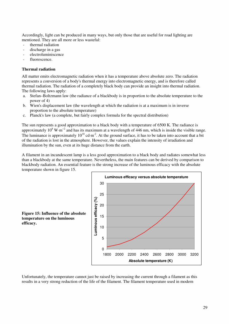
A filament in an incandescent lamp is a less good approximation to a black body and radiates somewhat less

than a blackbody at the same temperature. Nevertheless, the main features can be derived by comparison to

blackbody radiation. An essential feature is the strong increase of the luminous efficacy with the absolute

temperature shown in figure 15.

Figure 15: Influence of the absolute

temperature on the luminous

efficacy.

Unfortunately, the temperature cannot just be raised by increasing the current through a filament as this

results in a very strong reduction of the life of the filament. The filament temperature used in modern

30

standard lamps is in the range of 2800 to 2900 K. This, together with losses, explains that the luminous

efficacy of incandescent lamps is low.

Discharge in a gas

Gas-discharge lamps are light sources that generate light by sending an electrical discharge through an

ionized gas, a plasma. The principle is illustrated in figure 16.

Figure 16 The principle of generation of light by discharge in a gas.

The gas is enclosed in a tube with an electrical field applied between two electrodes. Free electrons

accelerate in the electrical field and collide with the atoms. Some electrons in the atomic orbitals of these

atoms are excited by these collisions to a higher energy state. When an excited electron falls back to a lower

energy state, it emits a photon of a characteristic energy.

The travel of the electrons in the electrical field represents the energy that is spent. The photons emitted

represent the luminous yield.

The gas in which the discharge takes place is either at a low pressure or at a high pressure.

By low pressure is meant that the gas is so rarified that the atoms do not interact with each other during

emission. Accordingly, the spectrum of the emitted light is the pure line spectrum of the particular gas.

By high pressure is meant that the lines of the spectrum are pressure broadening because of interaction

between the atoms. Most high pressure lamps for general lighting have pressures below the atmospheric

pressure and cause no danger of explosion. The exceptions are metal halide lamps.

Some gas discharge lamps use fluorescence to exchange photons of short wavelengths in the ultraviolet or

blue range to photons of longer wavelengths in the visible range. Fluorescence is introduced in 4.3.5.

Electroluminiscence

A diode consists of a chip of semiconducting material doped with impurities to create an excess of electrons

on one side and an excess of vacant states for electrons – called holes - on the other side. An electron has a

negative charge, while a hole acts like having a positive charge.

Once a diode is created, electrons and holes diffuse and meet at the junction between the two sides and

recombine in the sense that electrons fall into holes. This causes a lack of electrons and holes in a depletion

zone about the junction and simultaneously develops a voltage over this zone. The recombination of

electrons and holes stops when this voltage is sufficient to prevent diffusion through the zone. This voltage is

called the band voltage.

The current flows easily in one direction in a diode, but not in the reverse direction. Refer to figure 17 for

illustrations.

31

Figure 17: Construction of a semiconductor

diode, its depletion zone, current flow in one

direction, but not the other.

However, the current does flow in the reverse

direction if the voltage applied over the electrodes of the diode equals the band gap voltage and thereby

forces electrons and holes to meet and recombine. In this process, an electron receives an energy equal to the

charge of the electron multiplied with the band gap voltage, which it discharges as a photon with the same

energy.

This principle works for all diodes, but the particular matters of light emitting diodes (LED’s) are that the

generated photons have wavelengths in the visible range and that the construction of the diodes allows the

photons, or most of the photons, to escape.

The energy of a emitted photon E is given by its wavelength as λ= 1240 nm⋅eV/E eV, where λ is the

wavelength in nm. As an example, a band voltage of 2,48 V results in an energy of 2,48 eV of the photon

and a wavelength of 500 nm.

As the band voltage is characteristic of the semiconducting materials of the diode, a particular kind of LED

emits photons of a particular energy and thereby wavelength and colour.

It has been a substantial research and development work to arrive at different materials that produce light at

wavelengths ranging from the infrared over the colours of the visible spectrum to ultraviolet. Part of the

work has been to find materials and designs that allows the majority of the photons to escape the diode and

32

to create LED’s that can withstand a significant power without being destroyed the heating effects of the

current.

Over a period extending more than 30 years, the maximum luminous output of LED’s has been raised from

0,001 lm to now approaching 100 lm.

LED’s of the various signal colours like red, green and yellow have become the dominating light sources for

a large variety of signal lights.

However, white light is needed for lighting purposes. White light can in principle be composed of the light

from LED’s with different colours like red, green and blue, but the development has taken the way of using

blue light in combination with fluorescence to produce white light. Fluorescence is introduced in the next

section.

The available luminous flux per LED is sufficient for signal lights, but still small in view of the needs of road

lighting of perhaps 2 000 to 150 000 lm per light point. The development has gone in the direction of

combining a fairly large number of LED’s in modules, that do meet this need.

Fluorescence

Fluorescence is process in which a photon of a certain wavelength is absorbed in exchange for emission of a

photon of a longer wavelength.

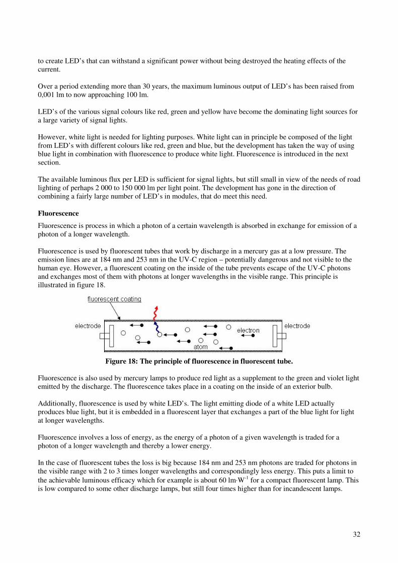
Fluorescence is used by fluorescent tubes that work by discharge in a mercury gas at a low pressure. The

emission lines are at 184 nm and 253 nm in the UV-C region – potentially dangerous and not visible to the

human eye. However, a fluorescent coating on the inside of the tube prevents escape of the UV-C photons

and exchanges most of them with photons at longer wavelengths in the visible range. This principle is

illustrated in figure 18.

Figure 18: The principle of fluorescence in fluorescent tube.

Fluorescence is also used by mercury lamps to produce red light as a supplement to the green and violet light

emitted by the discharge. The fluorescence takes place in a coating on the inside of an exterior bulb.

Additionally, fluorescence is used by white LED’s. The light emitting diode of a white LED actually

produces blue light, but it is embedded in a fluorescent layer that exchanges a part of the blue light for light

at longer wavelengths.

Fluorescence involves a loss of energy, as the energy of a photon of a given wavelength is traded for a

photon of a longer wavelength and thereby a lower energy.

In the case of fluorescent tubes the loss is big because 184 nm and 253 nm photons are traded for photons in

the visible range with 2 to 3 times longer wavelengths and correspondingly less energy. This puts a limit to

the achievable luminous efficacy which for example is about 60 lm⋅W-1 for a compact fluorescent lamp. This

is low compared to some other discharge lamps, but still four times higher than for incandescent lamps.

33

The loss is not so large for white LED’s, for which photons of 465 nm are traded for photons of 600 nm on

the average.

4.7 Light sources

Requirements for light sources

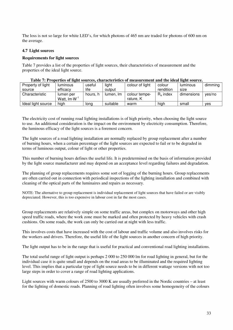
Table 7 provides a list of the properties of light sources, their characteristics of measurement and the

properties of the ideal light source.

Table 7: Properties of light sources, characteristics of measurement and the ideal light source. Property of light source

luminous efficacy

useful life

light output

colour of light colour rendition

luminous size

dimming

Characteristic lumen per

Watt, lm⋅W-1

hours, h lumen, lm colour tempe-rature, K

Ra index dimensions yes/no

Ideal light source high long suitable warm high small yes

The electricity cost of running road lighting installations is of high priority, when choosing the light source

to use. An additional consideration is the impact on the environment by electricity consumption. Therefore,

the luminous efficacy of the light sources is a foremost concern.

The light sources of a road lighting installation are normally replaced by group replacement after a number

of burning hours, when a certain percentage of the light sources are expected to fail or to be degraded in

terms of luminous output, colour of light or other properties.

This number of burning hours defines the useful life. It is predetermined on the basis of information provided

by the light source manufacturer and may depend on an acceptance level regarding failures and degradation.

The planning of group replacements requires some sort of logging of the burning hours. Group replacements

are often carried out in connection with periodical inspections of the lighting installation and combined with

cleaning of the optical parts of the luminaires and repairs as necessary.

NOTE: The alternative to group replacement is individual replacement of light sources that have failed or are visibly

depreciated. However, this is too expensive in labour cost in far the most cases.

Group replacements are relatively simple on some traffic areas, but complex on motorways and other high

speed traffic roads, where the work zone must be marked and often protected by heavy vehicles with crash

cushions. On some roads, the work can only be carried out at night with less traffic.

This involves costs that have increased with the cost of labour and traffic volume and also involves risks for

the workers and drivers. Therefore, the useful life of the light sources in another concern of high priority.

The light output has to be in the range that is useful for practical and conventional road lighting installations.

The total useful range of light output is perhaps 2 000 to 250 000 lm for road lighting in general, but for the

individual case it is quite small and depends on the road areas to be illuminated and the required lighting

level. This implies that a particular type of light source needs to be in different wattage versions with not too

large steps in order to cover a range of road lighting applications.

Light sources with warm colours of 2500 to 3000 K are usually preferred in the Nordic countries – at least

for the lighting of domestic roads. Planning of road lighting often involves some homogeneity of the colours

34

of light sources within a road network or an area for aesthetic reasons. For instance, light sources placed

close to each other or along a road should have similar colours of light.

It is generally agreed that colour rendition should be adequate on road areas that are lighted for pedestrians,

such as foot and cycle paths, domestic roads, pedestrians roads and even sidewalks and cycle paths along

traffic roads. In practice, priority has often been given to the efficiency of the road lighting, but this may

change with the availability of light sources with good colour rendition.

The luminous size of a light source has the significance that small dimensions allow optics that give better

control of the directionality of the light than large dimensions. Better control of the directionality has the

advantages of better aiming of the light towards the road areas to be illuminated and more freedom in the

lay-out of the lighting installations.

The development of optics for luminaires has actually gone hand in hand with the development of light

sources and has led to improvements of the lighting efficiency, the aesthetics of road lighting lay-out and

reductions of lighting nuisance such as undesirable lighting of properties and sky glow.

The possibility of dimming is an issue in those countries that use dimming at night for energy saving

purposes. All light sources can be dimmed in principle, but the equipment must be available and not too

complex and expensive. Additionally, the loss of luminous efficacy that is associated with dimming of most

light sources subtracts from the potential saving of energy and must not be too large.

Another matter not mentioned in table 7 is the prize of the lamps, ballasts and control gear. It is a trend that a

new type of lamp is more expensive than and older type of lamp and that this can affect the competition

between the two.

Light sources available for road lighting

Gas discharge lamps have had dominating use for road lighting in a long period. They can be divided into

two broad families based on discharge in gases with either sodium or mercury as the main components.

In each family there is a distinction between low pressure of the gas (low pressure sodium and fluorescent

lamps) and high pressure (high pressure sodium on one hand, and mercury and metal halide on the other

hand).

Fluorescent lamps may be subdivided into older types with rather large tube diameters and modern compact

fluorescent lamps.





produced by fluorescence. The metal halide lamps, on the other hand, do not rely of fluorescence.

Table 8 provides an account of the properties of light sources for road lighting. The account is indicative

only, as some of the properties vary with the wattages and subtypes of the lamps. Special versions with no or

little use for road lighting are not included in the table.

A red font is used where a property is unsatisfactory and a green font where it is acceptable or competitive

compared to other light sources. A black font means in between.

35

Table 8: Properties of light sources for road lighting. Property of light Source

luminous efficacy

useful life

light output

colour of light

colour rendition

Luminous size

dimming


Watt, lm⋅W-1

hours, h lumen, lm

colour temperature, K


Incandescent lamps 14 1 000 low 2800 K 100 small 1)

Gas discharge lamps

Low pressure sodium

High pressure sodium

Fluorescent tubes

Compact fluorescent

Mercury lamps

Metal halide CDM

Metal halide CPO

150

100

70

75

50

90

110

20 000

20 000

8 000

8 000

10 000

8 000

12 000

OK

OK

OK

OK 2)

OK

OK 2)

OK

false colour

2100 (false)

2900/4100

2700/4000

3500

3000

4000

0

25

51/63

82

50

80

65

large

small

large

medium

medium

small

small

1)

yes 1)

1)

yes

yes

yes

LED modules 100 30 000 OK OK 75 small yes

Ideal light source high long suitable warm high small yes 1)

Dimming has not been relevant for this lamp. 2)

The light output is in the lower end and sufficient for the lighting of domestic roads only.

The historical development of light sources has been in the sequence of incandescent lamps, gas discharge

lamps and LED modules. The gas discharge lamps are not quite listed in the sequence of historical

development – mercury lamps and fluorescent tubes in particular should be moved higher up in order to fit

that sequence.

However, with this in mind, table 8 does illustrate the historical development of road lighting and the quest

for better lighting economy in terms of higher luminous efficacy, longer useful life and better control of the

directionality of emitted light.

Incandescent lamps

Incandescent lamps were first, but are no longer used for road lighting and are included in table 8 for

historical reasons and for comparison only. They are not considered further.

The gas discharge lamps have competed with each other and supplemented each other for several decades.

The major competitors in later years have been high pressure sodium and metal halide lamps with some use

of compact fluorescent lamps for small installations.

Fluorescent tubes

The older types of fluorescent tubes are almost gone. Modern compact fluorescent tubes have some use for

the lighting of domestic areas, but will probably come under hard competition from LED modules.

Mercury lamps

The advantage of the mercury lamps compared to fluorescent tubes lies in the smaller dimensions of the

luminous parts. These are given by the approximately ellipsoidal shape of the exterior bulb. The size of the

ellipsoid depends on the lamp wattage. As an example, the width is 7,6 cm and the length is 12 cm for the

125 W lamp.

These dimensions are sufficiently small to allow for optics that direct the light both longitudinally and

transverse to the road so that use of large tilts and long arms can be avoided. This made the mercury lamps

popular for road lighting of traffic roads in a period ending with the advent of the far more efficient high

36

pressure sodium lamp. The mercury lamps kept its popularity for other road lighting purposes, such as the

lighting of domestic roads and city areas.

There is a process on eliminating the use of mercury lamps for road lighting and other lighting on the basis

of the Ecodesign or EuP Directive 2005/32/EC by the EU Commission. The long history of mercury lamps is

coming to an end.

Figure 19: A mercury lamp.

Low Pressure sodium lamps

Low pressure sodium lamps have had extensive use for road lighting on motorways and other large traffic

roads in some countries and some or very little or no use in other countries. The use is declining in view of

the poor quality of the light and competition from other light sources that can be supplied with efficient

optics.

Figure 20: A running low pressure sodium lamp.


The first high pressure sodium lamps came on the market in 1960’s, but with a wattage and a luminous

output too high for most road lighting applications. The 150 and 250 Watt lamps appeared late 1970’s with

luminous outputs suitable for road lighting of most traffic roads and they soon gained use as replacements for

250 and 400 W mercury lamps. The later addition of 50, 70 and 100 Watt lamps made the high pressure

sodium lamp the most ubiquitous lamp for street lighting on the planet.

High-pressure sodium lamps produce light by discharge in sodium at a higher pressure and with additional

elements such as mercury. On account of spectral pressure broadening and the emissions from mercury, the

spectrum has some coverage of colours. Because of the extremely high chemical activity of the high pressure

sodium arc, the arc tube is ceramic, made of translucent aluminium oxide.

Some advantages of high pressure sodium lamps are the same as for the low pressure sodium lamp, a high

efficacy and a long life. The luminous efficacy is about 100 lm⋅W-1 - and even higher for the high wattage

lamps.

The useful life is approximately 20 000 hours. It ends in a peculiar “cycling”, where a lamp turns itself off,

cools down, restarts, warms up etc.

An additional advantage is the small size of the luminous parts. The high pressure sodium lamps of suitable

wattages appeared first with frosted bulbs of the same elliptical shape and sizes as the mercury lamps they

were replacing. This allowed reuse of the optics developed for mercury lamps. Later versions with clear

bulbs allowed development of more efficient optics. Refer to figure 21.

High pressure sodium lamps can be dimmed individually by switching from the normal ballast to a ballast

with a higher reactive resistance. Another method with widespread use in Denmark is to reduce the voltage

to a group of lamps and luminaires by means of an autotransformer. The energy saving is approximately 35

% at a dimming level of 50 %.

37

Figure 21: A high pressure sodium lamp.

The colour of light is warm with a correlated colour temperature of 2100 K. The main disadvantages are that

the colour of light is a somewhat false yellow and that the colour rendition is poor with an Ra index of 25.

The main use of the high pressure sodium lamp is for road lighting of traffic road, but there is some use also

on domestic roads. This may be explained by the warm colour of light – even if the colour is not really nice.

Metal halide lamps

Metal halide lamps were not used, or at least not used much, for road lighting until the ceramic discharge

metal-halide (CDM) lamp emerged in the 1990’s. These lamps contain the discharge in ceramic tubes,

usually made of sintered alumina, similar to the ceramic tubes of the high pressure sodium lamps. The

advantage of the ceramic tubes, compared to fused quarts tubes, lies in their resistance to penetration by

metal ions.

The luminous efficacy of a CDM lamp is about 90 lm⋅W-1. The light is warm with a colour temperature of

3000 K. The colour rendition is good with an Ra index of approximately 80. The useful life is about 8 000

hours. The small ceramic tube is the luminous part.

Another more recent version of the ceramic discharge metal-halide lamp, the CPO lamp, has a higher

efficacy of 115 lm⋅W-1 and a longer useful life of about 12 000 hours. The cost of this is a higher colour

temperature of 4000 K and a somewhat lower Ra index of 60 to 70. This lamp is a real competitor to the high

pressure sodium lamp. A CPO lamp is shown in figure 22.

Figure 22: A metal halide lamp (CPO).

LED modules

LED modules of a luminous efficacy of 100 lm⋅W-1, a useful life of 30 000 hours, a reasonably good colour

of light and an Ra index of 75 are available. However, LED’s in general - and white LED’s in particular - are

still being improved.

LED modules represent a break through into a light source with good qualities in all respects. The lighting

world has been waiting – waiting - and waiting for this. The difficulties of developing the LED’s themselves

and the LED modules must have been severe. But now they are here and the potential for further

development is high.

There might be a day, where the LED module is the only light source for road lighting. Unless something

else is invented – there are many ways to produce light.

Figure 23: An LED module placed in a conventional housing.

38

39

6. Luminaires for road lighting


A luminaire has a housing with a fixing device and includes a socket for a light source, gear to start and

operate the light source, electrical terminals and cables, optics to direct the light from the light source, an

aperture through which the light can pass and a transparent screen covering the aperture.

The fixing device can be designed for mounting on the top of a lighting column, on a bracket extending from

a lighting column or in a wire suspension.

Most luminaires have one light source, but some have more than one. The gear to start and operate a light

source can be a starter and a magnetic ballast or it can be an electronic ballast. Some luminaires also include

gear for dimming and communication.

Optics to direct the light can be white surfaces, louvres, transilluminated surfaces with diffusing or light

scattering properties, mirror optics or refracting optics etc.

The aperture can be plane or have other shapes like cylinders, cones and spheres. The screen covering a

plane aperture can itself be plane, or it can curve or have the shape of a bowl. Some screens are clear and

some have properties of diffusion, light scattering or refraction. Some luminaires have apertures in addition

to main apertures that serve to illuminate the luminaires themselves.

Luminaires based on Light Emitting Diodes LED’s may have an LED module that integrates an electronic

ballast and optics to direct the light.

Optics for luminaires are discussed in 4.2, where distinction is made between simple optics, mirror optics

and optics of LED modules. Mirror optics are divided into “parabolic” and “pot” optics. Most luminaires

with mirror optics have setting options for the directionality of the emitted light by marked positions of the

light source or of the mirrors.

Optics of luminaires are intended to shape the directionality of the emitted light and to control glare.

The directionality of emitted light is described by means of light distributions that map the luminous

intensity in directions relative to the luminaires. Light distributions are tables in an angular system of two

angles that are placed in files and made available for design calculations of road lighting installations.

Light distributions are described in 4.3, with some detail provided for the conventional angular system, for

methods of measurement and for conventions regarding orientation of luminaires in design calculations.

Additionally, the polar diagram used to visualize the directionality of the light by means of curves is

explained, and some typical examples of light distributions are presented.

The luminaire cut-off classes G*1, G*2, G*3, G*4, G*5 and G*6 as defined in EN 13201-2 are introduced in

4.4. These classes are intended for luminaires at traffic roads and are relevant for the control of disability

glare of drivers and also for the control of lighting nuisances such as undesirable lighting of properties,

intrusions into the night scene at long distance and illumination of the sky.

In annex A it is demonstrated that use of luminaires of the higher classes G*4, G*5 and G*6 does ensure

relatively low levels of disability glare as measured by the Threshold Increment TI. The classes may also be

applied for luminaires at domestic roads.

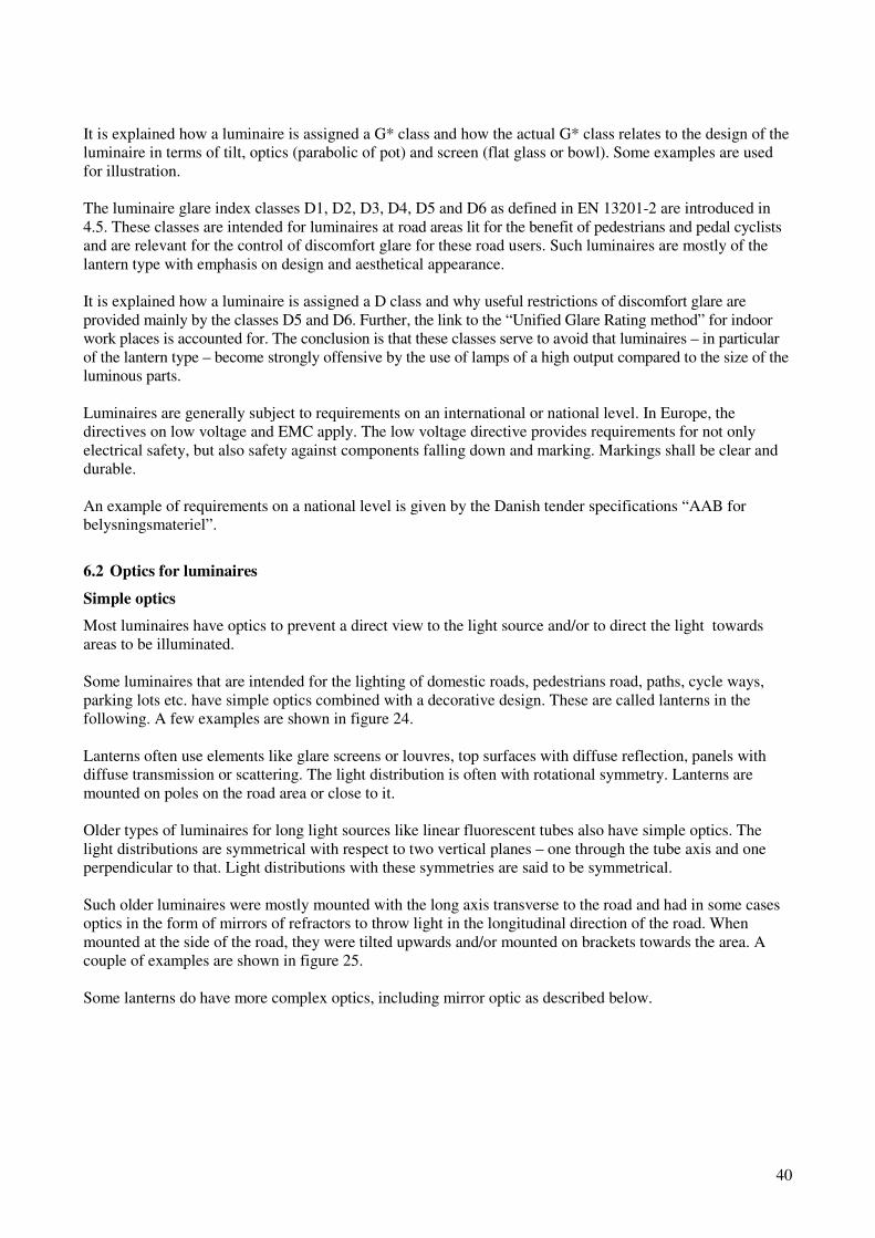
40

It is explained how a luminaire is assigned a G* class and how the actual G* class relates to the design of the

luminaire in terms of tilt, optics (parabolic of pot) and screen (flat glass or bowl). Some examples are used

for illustration.

The luminaire glare index classes D1, D2, D3, D4, D5 and D6 as defined in EN 13201-2 are introduced in

4.5. These classes are intended for luminaires at road areas lit for the benefit of pedestrians and pedal cyclists

and are relevant for the control of discomfort glare for these road users. Such luminaires are mostly of the

lantern type with emphasis on design and aesthetical appearance.

It is explained how a luminaire is assigned a D class and why useful restrictions of discomfort glare are

provided mainly by the classes D5 and D6. Further, the link to the “Unified Glare Rating method” for indoor

work places is accounted for. The conclusion is that these classes serve to avoid that luminaires – in particular

of the lantern type – become strongly offensive by the use of lamps of a high output compared to the size of the

luminous parts.

Luminaires are generally subject to requirements on an international or national level. In Europe, the

directives on low voltage and EMC apply. The low voltage directive provides requirements for not only

electrical safety, but also safety against components falling down and marking. Markings shall be clear and

durable.

An example of requirements on a national level is given by the Danish tender specifications “AAB for

belysningsmateriel”.

6.2 Optics for luminaires

Simple optics

Most luminaires have optics to prevent a direct view to the light source and/or to direct the light towards

areas to be illuminated.

Some luminaires that are intended for the lighting of domestic roads, pedestrians road, paths, cycle ways,

parking lots etc. have simple optics combined with a decorative design. These are called lanterns in the

following. A few examples are shown in figure 24.

Lanterns often use elements like glare screens or louvres, top surfaces with diffuse reflection, panels with

diffuse transmission or scattering. The light distribution is often with rotational symmetry. Lanterns are

mounted on poles on the road area or close to it.

Older types of luminaires for long light sources like linear fluorescent tubes also have simple optics. The

light distributions are symmetrical with respect to two vertical planes – one through the tube axis and one

perpendicular to that. Light distributions with these symmetries are said to be symmetrical.

Such older luminaires were mostly mounted with the long axis transverse to the road and had in some cases

optics in the form of mirrors of refractors to throw light in the longitudinal direction of the road. When

mounted at the side of the road, they were tilted upwards and/or mounted on brackets towards the area. A

couple of examples are shown in figure 25.

Some lanterns do have more complex optics, including mirror optic as described below.

41

Figure 24: Examples of lanterns.

Figure 25: Examples of luminaires with

fluorescent tubes.

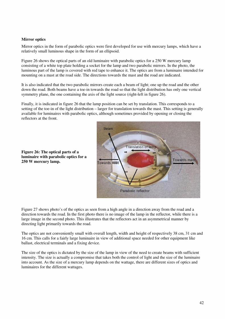
42

Mirror optics

Mirror optics in the form of parabolic optics were first developed for use with mercury lamps, which have a

relatively small luminous shape in the form of an ellipsoid.

Figure 26 shows the optical parts of an old luminaire with parabolic optics for a 250 W mercury lamp

consisting of a white top plate holding a socket for the lamp and two parabolic mirrors. In the photo, the

luminous part of the lamp is covered with red tape to enhance it. The optics are from a luminaire intended for

mounting on a mast at the road side. The directions towards the mast and the road are indicated.

It is also indicated that the two parabolic mirrors create each a beam of light; one up the road and the other

down the road. Both beams have a toe-in towards the road so that the light distribution has only one vertical

symmetry plane, the one containing the axis of the light source (right-left in figure 26).

Finally, it is indicated in figure 26 that the lamp position can be set by translation. This corresponds to a

setting of the toe-in of the light distribution – larger for translation towards the mast. This setting is generally

available for luminaires with parabolic optics, although sometimes provided by opening or closing the

reflectors at the front.

Figure 26: The optical parts of a

luminaire with parabolic optics for a

250 W mercury lamp.

Figure 27 shows photo’s of the optics as seen from a high angle in a direction away from the road and a

direction towards the road. In the first photo there is no image of the lamp in the reflector, while there is a

large image in the second photo. This illustrates that the reflectors act in an asymmetrical manner by

directing light primarily towards the road.

The optics are not conveniently small with overall length, width and height of respectively 38 cm, 31 cm and

16 cm. This calls for a fairly large luminaire in view of additional space needed for other equipment like

ballast, electrical terminals and a fixing device.

The size of the optics is dictated by the size of the lamp in view of the need to create beams with sufficient

intensity. The size is actually a compromise that takes both the control of light and the size of the luminaire

into account. As the size of a mercury lamp depends on the wattage, there are different sizes of optics and

luminaires for the different wattages.

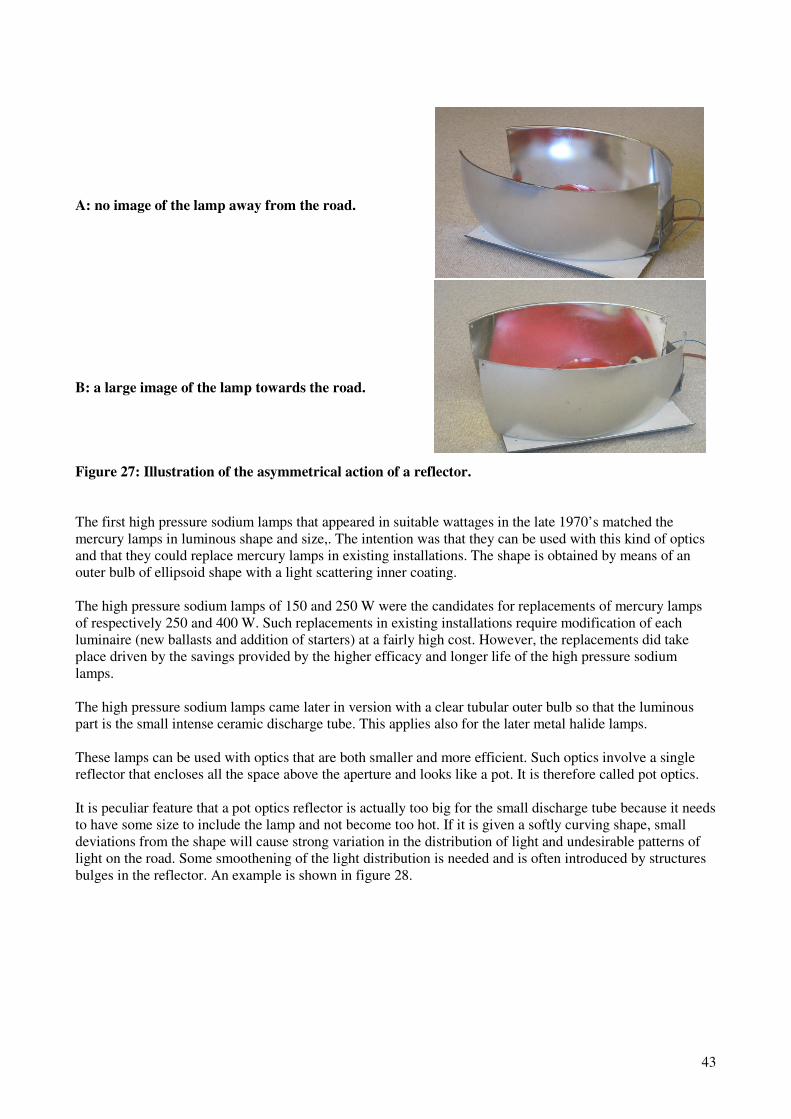
43

A: no image of the lamp away from the road.

B: a large image of the lamp towards the road.

Figure 27: Illustration of the asymmetrical action of a reflector.

The first high pressure sodium lamps that appeared in suitable wattages in the late 1970’s matched the

mercury lamps in luminous shape and size,. The intention was that they can be used with this kind of optics

and that they could replace mercury lamps in existing installations. The shape is obtained by means of an

outer bulb of ellipsoid shape with a light scattering inner coating.

The high pressure sodium lamps of 150 and 250 W were the candidates for replacements of mercury lamps

of respectively 250 and 400 W. Such replacements in existing installations require modification of each

luminaire (new ballasts and addition of starters) at a fairly high cost. However, the replacements did take

place driven by the savings provided by the higher efficacy and longer life of the high pressure sodium

lamps.

The high pressure sodium lamps came later in version with a clear tubular outer bulb so that the luminous

part is the small intense ceramic discharge tube. This applies also for the later metal halide lamps.

These lamps can be used with optics that are both smaller and more efficient. Such optics involve a single

reflector that encloses all the space above the aperture and looks like a pot. It is therefore called pot optics.

It is peculiar feature that a pot optics reflector is actually too big for the small discharge tube because it needs

to have some size to include the lamp and not become too hot. If it is given a softly curving shape, small

deviations from the shape will cause strong variation in the distribution of light and undesirable patterns of

light on the road. Some smoothening of the light distribution is needed and is often introduced by structures

bulges in the reflector. An example is shown in figure 28.

44

Figure 28: Example of pot optics.

The toe-in of the light distribution is set by translation of the lamp as with parabolic optics. Some luminaires

also offer alternative height positions of the lamps corresponding to lifting of lowering the beams of light (a

higher positions means lowering the beams and vice versa).

It took some years before efficient pot optic reflectors were available; this was probably by late 1980’s.

As the technique of providing reflectors with surfaces of high reflection had been developed at this point in

time, pot optics raised the efficiency of luminaires from typically 70 % to 80 %. The improvement in lighting

efficiency is higher because of the improved control of the directionality of the light.

Luminaires with reflector optics are used not only on traffic roads, but also on domestic roads and other road

areas for pedestrians and cyclists, where they compete with lanterns.

Optics for LED modules

It may some day be possible to make a compact light source based on LED’s that can be used with optics as

described above. With the present technology, it is necessary to use several LED’s placed in arrays that are a

bit large for use with reflectors.

Therefore, the light from each LED is often directed individually, with each LED forming a beam of some

width shaped by refracting and/or reflecting optics. The complete light distribution is added up by the beams

from the individual LED’s. There are probably several variations of this theme on the market, and new

variations being developed.

The first LED luminaires used pointing of the LED’s and their optics. This raises the problem in connection

with road lighting of traffic roads that there is a need to set the light distributions to match the need for the

individual installations.

At least one of the solutions is elegant. It is to mount the LED’s in a matrix and provide a plate with

individual refractive optics for each of the LED’s. The optics plate determines the light distribution and

change of the optics plate changes the light distribution. It is probably expensive to develop a sufficient

number of optics plates, but cheap to produce them by moulding.

6.3 Light distributions of luminaires

General about light distributions

A light distribution of a luminaire is a mapping of the luminous intensities of the luminaire in directions

relative to the luminaire. The somewhat longer and more correct designation is “luminous intensity

distribution”.

45

A light distribution table is generally placed in a file together with some information of the luminaire.

Several file formats have been used over the years, but a free program for lighting design calculation has

become so popular that its file format has become dominating in Europe. This the DIALux program; the file

format is called EULUMDAT. The files can be opened for inspection with programs like Notebook and

Microsoft Excel.

The values of the table are normally not the luminous intensities I in the unit of candela (cd), but the

proportions between I and the light output of the light source(s) installed in the luminaire Φlight source. The light

output of the light source(s) is measured in kilolumens (klm) and, accordingly, the unit of the values of the

table is candela per kilolumen (cd/klm).

This has the simple advantage that the values can be integers ranging from 0 up to typically a few hundreds.

The major advantage is, however, that the light distribution does not incorporate the light output of the light

sources and can be used in combination with light sources of different light outputs, when relevant.

Relevant cases can for instance be mercury lamps and high pressure sodium lamps with the same luminous

shape and size. The same light distribution table applies, but with different light outputs of the light sources.

The exception from this scaling of the values of the table is formed by luminaires using LED modules. In

these, the LED’s are inseparable from the optics and the power supplies, so that it has no meaning to identify

a light output of the LED’s themselves. For such luminaires the values of the table are directly the luminous

intensities in the unit of candela (cd). The term used is the rather drastic “absolute photometry”.

In geometrical terms, a luminaire is represented by an optical centre and three axes. Refer to figure 29.

Figure 29: The optical centre and three axes of a luminaire.

The optical centre is in the midpoint of the optical parts of the luminaire.

The axes point from the geometrical centre and are perpendicular to each other and have directions so that

the vector product of axes 1 and 2 point into the direction of axis 3. Because of this, the vector product of

axes 2 and 3 points into the direction of axes 1, and the vector product of axes 3 and 1 points into the

direction of axis 2.

The axis 1 is vertical and point downwards, when the luminaire is in the normal orientation. Axis 2 is

selected as a horizontal direction by:

- random selection, when the luminaire has rotational symmetry

- along the long direction of the light source(s), when the luminaire is symmetrical (two vertical

symmetry planes at right angles to each other)

- in the asymmetrical lighting direction, when the luminaire is asymmetrical (one vertical symmetry

plane).

Axis 3 is determined by the selections of axes 1 and 2.

46

With the starting point in these axes, directions relative to the luminaire are given by two angles C and γ in

an angular co-ordinate system (C,γ). Refer to the illustration in figure 30.

Figure 30: Definition of a direction relative to a

luminaire by two angles C and γγγγ.

It is common that light distribution tables have uniform steps in the angles C and γ, for instance 5° steps in C

and 2° steps in γ.

The angle C ranges in principle from 0° to 360°, for instance in the steps of 0°, 5°, 10° ... 355°. All these

values are included in the measurement resulting in an initial table, but the range is often reduced in

accordance with the symmetry of the luminaire in a final table:

- to a single value of C for luminaires of rotational symmetry (about a vertical axis)

- to a range from 0° to 90° for symmetrical luminaires (two vertical symmetry planes)

- to a range from -90° to 90° for asymmetrical luminaires (one vertical symmetry plane).

In this way, a symmetry is forced into the final table even if it may not quite be inherent in the initial table.

This is convenient, because a designer of lighting installations may expect the symmetry to prevail in the

results of calculations and would be puzzled if it isn’t.

Deviations from symmetry may be due to random variations. In other cases there are details of the structure

of a luminaire that are not quite symmetrical, but nevertheless ignored by a conventional assumption of

symmetry.

The angle γ ranges in principle from 0° to 180°, for instance in the steps of 0°, 2°, 4° ... 180°. However, in

cases where there is no light above a particular value of γ, the upper end of the range is sometimes reduced to

that value of γ.

The C, γ angles are similar to the latitude and longitude of the globe, although with a start of γ at 0° at the

south pole, the middle at 90° at the equator and an end at 180° at the north pole. Refer to figure 31.

47

Figure 31: The C, γγγγ angles drawn on a sphere with

indications of some directions.

As indicated in figure 31, each direction can be assigned an area of the sphere corresponding to a solid angle

dω. As the luminous intensity I is also available for the particular direction, it can be assigned a luminous

flux of dΦ= I×dω. The total light output Φoutput is obtained as the sum of dΦ over all the directions of the

light distribution.

The ratio between the total light output and the luminous flux of the light source is the efficiency of the

luminaire µ given by µ = Φoutput /Φlight source. The efficiency is often called the Light Output Ratio abbreviated

LOR.

When the values of the luminous intensity table are relative in the unit of candela per kilolumen, the

calculated value of Φoutput is 1000 times the efficiency, i.e. the efficiency measured per thousand.

The efficiency is of course an important characteristic of a luminaire. It is often split up in two components

involving light emitted up to γ = 90° and above γ = 90° and called respectively Lower Light Output Ratio

LLOR and Upper Light Output Ratio ULOR.

In case of absolute photometry of luminaires with LED modules, there is no values of Φoutput to refer to, and a

value of the efficiency cannot be determined. The value can formally be set to 1 or 100 %, but this does not

imply that LED modules are without losses.

Measurement of light distributions

A light distribution can be measured in a photometer bench with a goniometer and a photometer placed at a

sufficient distance along the bench as shown in figure 32.

Figure 32: A photometer bench with a

photometer and a goniometer.

48

The luminaire is mounted in a specific manner in the goniometer after which the angles C and γ are set by

rotations about respectively the second and the first rotation axes of the goniometer.

This method has the disadvantage that some light sources change their light output when being tilted. This

introduces the need for compensation by means of some additional measurements.

It is better to measure the light distribution in a special light distribution photometer, where the luminaire is

not tilted. The most widespread type is the rotating mirror photometer in which the luminaire is rotated about

a vertical axis (not changing tilt) and a large mirror rotates around the luminaire about a horizontal axis. The

measurements take place through the mirror, which shows different views of the luminaire when rotating.

Such a photometer is illustrated in figure 33.

Figure 33: A rotating mirror light distribution photometer.

A rotating mirror photometer also has two rotation axis. One is vertical, about which the luminaire is rotated,

and the other is horizontal about which the mirror is rotated. The angles C and γ are set by rotations of

respectively the luminaire and the mirror.

Polar diagrams

Polar diagrams are often used to illustrate light distributions by means of luminous distribution curves.

A curve applies for luminous intensities in directions in a vertical half plane through the optical centre of the

luminaire. The vertical half plane is defined by a value of the angle C. The curve shows the table value at

each value of γ in the way indicated in figure 34. The diagram is equipped with concentric circles with radii

that reflect steps of values, for instance 0, 50, 100, 150 and 200 cd/klm, and a set of lines through the optical

centre that reflect steps of γ, for instance 0°, 15°, 30°, 45° ... 180°.

Figure 34: A polar diagram with a light distribution

curve.

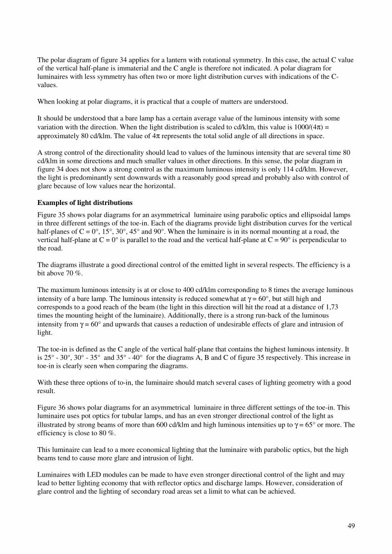
49

The polar diagram of figure 34 applies for a lantern with rotational symmetry. In this case, the actual C value

of the vertical half-plane is immaterial and the C angle is therefore not indicated. A polar diagram for

luminaires with less symmetry has often two or more light distribution curves with indications of the C-

values.

When looking at polar diagrams, it is practical that a couple of matters are understood.

It should be understood that a bare lamp has a certain average value of the luminous intensity with some

variation with the direction. When the light distribution is scaled to cd/klm, this value is 1000/(4π) =

approximately 80 cd/klm. The value of 4π represents the total solid angle of all directions in space.

A strong control of the directionality should lead to values of the luminous intensity that are several time 80

cd/klm in some directions and much smaller values in other directions. In this sense, the polar diagram in

figure 34 does not show a strong control as the maximum luminous intensity is only 114 cd/klm. However,

the light is predominantly sent downwards with a reasonably good spread and probably also with control of

glare because of low values near the horizontal.

Examples of light distributions

Figure 35 shows polar diagrams for an asymmetrical luminaire using parabolic optics and ellipsoidal lamps

in three different settings of the toe-in. Each of the diagrams provide light distribution curves for the vertical

half-planes of C = 0°, 15°, 30°, 45° and 90°. When the luminaire is in its normal mounting at a road, the

vertical half-plane at C = 0° is parallel to the road and the vertical half-plane at C = 90° is perpendicular to

the road.

The diagrams illustrate a good directional control of the emitted light in several respects. The efficiency is a

bit above 70 %.

The maximum luminous intensity is at or close to 400 cd/klm corresponding to 8 times the average luminous

intensity of a bare lamp. The luminous intensity is reduced somewhat at γ = 60°, but still high and

corresponds to a good reach of the beam (the light in this direction will hit the road at a distance of 1,73

times the mounting height of the luminaire). Additionally, there is a strong run-back of the luminous

intensity from γ = 60° and upwards that causes a reduction of undesirable effects of glare and intrusion of

light.

The toe-in is defined as the C angle of the vertical half-plane that contains the highest luminous intensity. It

is 25° - 30°, 30° - 35° and 35° - 40° for the diagrams A, B and C of figure 35 respectively. This increase in

toe-in is clearly seen when comparing the diagrams.

With these three options of to-in, the luminaire should match several cases of lighting geometry with a good

result.

Figure 36 shows polar diagrams for an asymmetrical luminaire in three different settings of the toe-in. This

luminaire uses pot optics for tubular lamps, and has an even stronger directional control of the light as

illustrated by strong beams of more than 600 cd/klm and high luminous intensities up to γ = 65° or more. The

efficiency is close to 80 %.

This luminaire can lead to a more economical lighting that the luminaire with parabolic optics, but the high

beams tend to cause more glare and intrusion of light.

Luminaires with LED modules can be made to have even stronger directional control of the light and may

lead to better lighting economy that with reflector optics and discharge lamps. However, consideration of

glare control and the lighting of secondary road areas set a limit to what can be achieved.

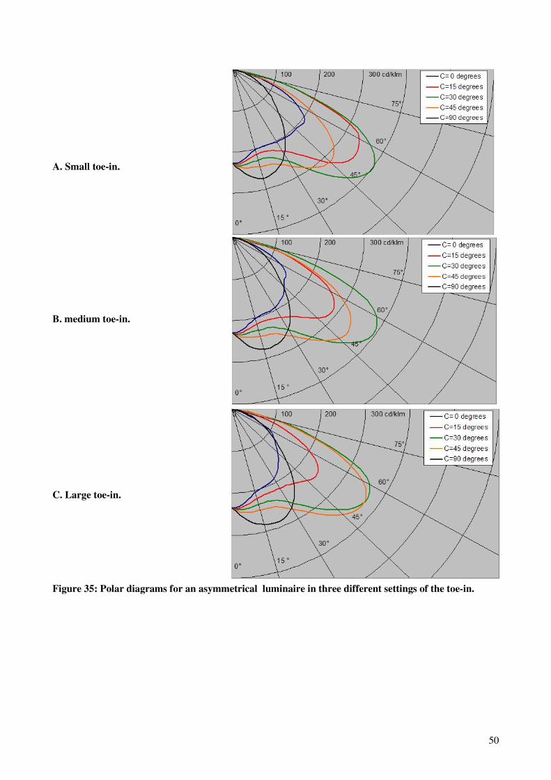
50

A. Small toe-in.

B. medium toe-in.

C. Large toe-in.

Figure 35: Polar diagrams for an asymmetrical luminaire in three different settings of the toe-in.

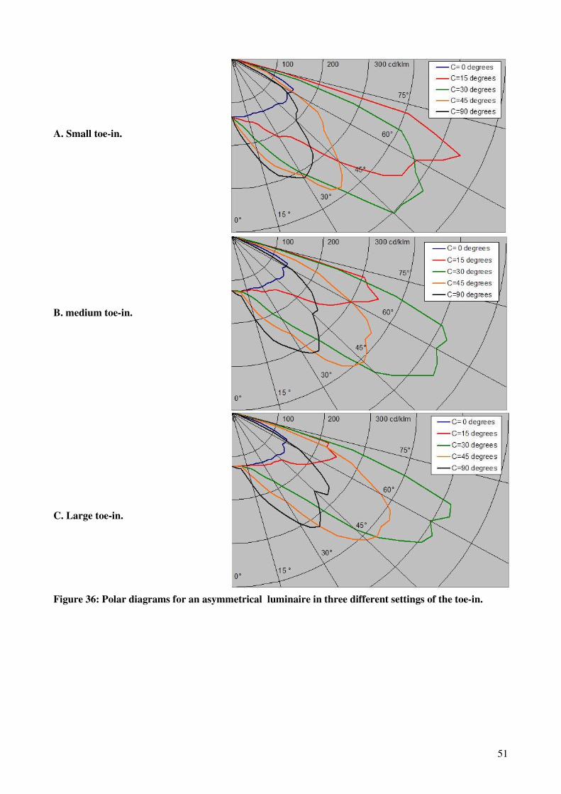
51

A. Small toe-in.

B. medium toe-in.

C. Large toe-in.

Figure 36: Polar diagrams for an asymmetrical luminaire in three different settings of the toe-in.

52

6.4 Luminous intensity classes

Table A.1 of EN 12301-2 defines luminous intensity classes for luminaires as installed. This table is shown

in table 9.

Table 9: Luminous intensity classes.

Class Maximum proportion between the luminous intensity and the luminous flux emitted in directions below the horizontal in cd/klm

Other requirements

at 70° a at 80°

a at 90°

a

G*1 200 50 None

G*2 150 30 None

G*3 100 20 None

G*4 500 100 10 Luminous intensities above 95° a) to be zero



a Any direction forming the specified angle from the downward vertical, with the luminaire installed for use.

b Luminous intensities up to 1 cd/klm can be regarded as being zero.

By luminous intensity classes for luminaires as installed is meant that the characteristic values used in table 9

are to be determined for the actual tilt with which the luminaire is mounted.

When a light distribution table is available for the actual tilt, the procedure is as follows:

a. the luminous flux in the lower hemisphere is determined by the method of summation that has been

accounted for in 6.3.1

b. this luminous flux is converted to kilolumens (klm) by division with 1000 lm/klm

c. all the values of the table are rescaled by division with the converted luminous flux

d. the rescaled values are compared to the maximum values indicated in table 9.

The classes G*1, G*2, G*3, G*4, G*5 and G*6 reflect increasing requirements for cut-off of the luminous

intensities at directions at the horizontal (90°), close below the horizontal (70° and 80°) or above. The

requirements are expressed by maximum proportions between the luminous intensity and the total light

output in the lower hemisphere.

The classes are intended for luminaires at traffic roads and are relevant for the control of glare of drivers and

also for the control of lighting nuisances such as undesirable lighting of properties, intrusions into the night

scene at long distance and illumination of the sky. It is demonstrated in the annex A that use of luminaires of

the higher classes G*4, G*5 and G*6 does ensure relatively low levels of disability glare as measured by the

Threshold Increment TI. The classes may also be applied for luminaires at domestic roads.

The classes G*1, G*2 and G*3 correspond to "semi cut-off" and "cut-off" concepts of traditional use with

requirements, however, modified to suit the prevailing use of light sources and luminaires. The luminaires

shown in figure 37 may be of these classes.

53

A: Luminaire with fluorescent tubes.

B: Luminaire with parabolic optics and a bowl.

C: Luminaire with a flat glass and a shirt.

Figure 37: Some luminaires with weak cut-off in the classes G*1, G*2 and G*3.

The classes G*4, G*5 and G*6 correspond to a strong cut-off as obtained with luminaires with little or no tilt

and flat glass screens of the light aperture. The luminaires shown in figure 38 may be of these classes.

A: Luminaire with pot optics and a flat horizontal glass.

B: Luminaire with an LED module and a flat horizontal glass.

Figure 38: Luminaires with strong cut-off in the classes G*4, G*5 or G*6.

54

6.5 Glare index classes

Table A.2 of EN 12301-2 defines glare index of luminaires. This table is shown in table 10.

Table 10: Glare index classes

Class D0 D1 D2 D3 D4 D5 D6

Glare index maximum – 7000 5500 4000 2000 1000 500

The glare index is I ×A-0,5

where I is the maximum value of the luminous intensity measured in candela (cd) in any direction

forming an angle of 85° from the downward vertical

and A is the apparent area in square metres (m2) of the luminous parts of the luminaire on a

plane perpendicular to the direction of I

The unit of the glare index is cd/m.

The value of I can be obtained from the light distribution of the luminaire. It has to be an absolute value in

candela (cd). The value of A can be derived from the luminous shape of the luminaire.

EXAMPLE: A luminaire with a circular horizontal light aperture of a diameter

D has an apparent area found by A = cos(85°)×π×D2/4 = 0,068×D

2.

The classes are intended for luminaires at road areas lit for the benefit of pedestrians and pedal cyclists and are

relevant for the control of discomfort glare for these road users. Such luminaires are mostly of the lantern

type with emphasis on design and aesthetical appearance.

It is an assumption that the optics of the lantern prevent a direct view of the light source in the direction of

the luminous intensity I by means of shielding or surfaces of some diffusion or scattering. Therefore, it is a

rule that class D0 applies if parts of the light source are visible in this direction.

However, when the EN 13201 series were first drafted during the 1990’s, scepticism among some of the

participants led to the inclusion of the classes D1, D2, D3 and partly D4 of high glare index values. Bare

ellipsoidal lamps of the lower wattages would be very unpleasant in the night scene, but are nevertheless

allowed by the classes. 50 and 70 W high pressure sodium lamps fit into D2 and D1 respectively, while bare

50 and 80 W mercury lamps fit into D3 and D2 respectively.

Therefore, useful restrictions of discomfort glare are provided mainly by the classes D5 and D6.

The glare index represents a strongly simplified version of the “Unified Glare Rating method” used for indoor

work places cannot be expected to provide an accurate impression of discomfort glare. However, the classes

serve to avoid that luminaires – in particular of the lantern type – become strongly offensive by the use of

lamps of a high output compared to the size of the luminous parts of the luminaire. The UGR method is

described in CIE 117 “Discomfort glare in interior lighting”.

55

7. Lighting installations


As a part of designing a road lighting installation, the installation needs to be described and documented.

This is considered in 7.2 in terms of road areas and lighting requirements, installation components and data

and finally installation geometry. A complete documentation would include guides for operation and

maintenance.

In 7.3 it is pointed out that national regulations, standards and tender specifications may provide

requirements for lighting installations with a view to their day time appearance, night time appearance and

comfort and minimizing light emitted in directions where it is neither necessary nor desirable. Such

requirements relate to national traditions with emphasis on particular aspects of road lighting. Additional

requirements may relate to energy efficiency.

Energy efficiency is an aspect that may gain particular and increasing attention. A simple measure of energy

efficiency is accounted for in 7.4. Ongoing work (Spring 2013) on a prEN 12352-5 “Road Lighting – Part 5:

Energy Performance in Road Lighting” follows related principles, while the above-mentioned measure is

included in a normative annex.

7.2 Description of lighting installations

Road areas and lighting requirements

Some road lighting installations provide road lighting for the benefit of drivers of motorized vehicles on one

or more carriageways and in addition provide road lighting on side areas. The side areas may include

pedestrian side walks, cycle lanes, emergency lanes or just plain areas next to the carriageway. The lighting

of these areas may be for the benefit of pedestrians, cyclists, drivers with an emergency stop, or just to

enable drivers on the carriageway to see persons or animals about to enter the carriageway.

Other road lighting installations provide lighting for the benefit of pedestrians and cyclists on a road area that

may comprise a pedestrian path, a cycle path, a domestic road, a parking lot or a pedestrian zone. Drivers of

motorized vehicles on these areas have to drive slowly and find their way with assistance of the vehicle

headlamps.

Therefore, one set of lighting requirements may apply for the carriageway with additional sets of

requirements for the side areas, or one set of lighting requirements apply for the whole road area.

An account for the road areas and the lighting requirements is a necessary part of a description of a lighting

installation. The road areas are to be accounted for in geometrical terms, while the lighting requirements are

to be accounted for in terms of lighting classes such a provided in EN 13201-2.

The geometry of road areas may sometimes be simple, for instance that a traffic road has a single

carriageway of a particular width and side areas of a different width, or that a domestic road has a particular

total width. In other cases, it may be necessary to provide an additional account for curve of a road, or for a

road area of complex shape in a global co-ordinate system.

The road areas and the lighting requirements may be subject to national standardisation or regulation.

Installation components and data

The main installation components include foundations, lighting columns, arms, brackets, wire suspensions,

luminaires and light sources. These should be accounted for in terms of manufacturers, types, dimensions,

56

passive safety, settings of luminaires, light distributions of luminaires, classes of luminaires, types and

properties of light sources etc.

When the lighting requirements are based on road surface luminance, such as for the M classes of EN 12352-

2, the reflection properties of the road surface is terms of standard road reflection table and Q0 (or Qd) value

must be specified as well. The specification must include the standard reflection table for the wet condition,

when an additional requirement is applied for the wet condition.

Electrical and electronic equipment for the power supply, electrical connections, monitoring and dimming of

the lighting installation should be accounted for as well. The account should include annual hours in normal

and dimmed operation and the power consumptions in these states of operation.

Finally, the assumptions regarding maintenance and the value selected for the maintenance factor should be

accounted for.

Lighting columns, arms and brackets are covered by the EN 40 series. These involve CE marking.

Installation components may be subject to national standardisation and tender specifications.

EXAMPLE: Danish road lighting standards specify use of road reflection table N2 with a Q0 of 0,09 (expressed by the

equivalent value for Qd of 0,078) for the dry condition and standard road reflection table W4 for the wet condition.

These specifications are based on tender specifications for road surfaces on roads with road lighting.

Installation geometry

The luminaires of lighting installations are mounted on columns, either directly on the top of the columns or

on arms or brackets extending from the columns, or they are suspended in wires stretched between the

columns.

On longitudinal stretches of road, the luminaires are generally mounted in one or more rows along the road.

The typical arrangements for column mounting are shown in shown in figure 39. The luminaire spacing, as

measured on one road side, is indicated.

The single sided arrangement has relatively few luminaires and thereby relatively low installation and

maintenance costs. It is the preferred arrangement for narrow roads.

In case of wider roads, the double sided arrangement is often preferred. Its two rows of luminaires add to the

installation and maintenance costs, but not quite to a factor of two compared to the single sided arrangement

as the spacing between luminaires can generally be larger.

In some cases, the staggered arrangement is preferred instead of the double sided arrangement as it often

allows a larger luminaire spacing than the double sided arrangement. The disadvantage is that this

arrangement has a poor optical guidance by the luminaires – in particular on curved roads.

On roads with a central reserve separating two road areas, the twin central installation with two luminaires

on each column is mostly preferred. This arrangement can be used with a fairly large luminaire spacing, and

it provides good use of the light output. The disadvantage on high speed roads, such as motorways, lies in the

difficulty of getting access to the luminaires for maintenance.

57

Figure 39: Arrangements of column mounted luminaires.

At other road areas, such as at intersections, roundabouts, squares, parking lots etc. the luminaires are

mounted so as to match the geometry of the road area and the lighting criteria. At intersections and

roundabouts, the number of columns is often kept low by mounting two or more luminaires on each column.

The luminaires can have different orientations, settings and even wattages. Some countries use high mast

lighting at complex motorway junctions with several narrow beam luminaires at the top of each mast.

Wire suspension of the luminaires was used widely in early road lighting based on fluorescent tubes and

mercury lamps in order to bring luminaires with poor control of the light over the road areas. This kind of

lighting has generally been replaced.

Wire suspension is still used in some city areas with lack of space in order to reduce the number of columns

or avoid them by stretching the wires between buildings. There are also cases of use of wire suspension at

roundabouts in order to place the columns at a safe distance from the road area.

A particular type of wire suspension called catenary lighting has in some cases been used for motorway

lighting. The characteristic feature is that high and strong columns at large spacing in the central reserve

carry several luminaires in between them. Catenary lighting has a good optical guidance by showing

luminaires like pearls on a string along the road. The disadvantage is a relatively high cost of the suspension

arrangement and intrusion into the visual scene at both day and night.

NOTE: Catenary lighting was the standard solution for early motorway lighting in the Copenhagen area, some of

remains by 2013.

A luminaire arrangement is described by its type of arrangement as described above, and by some additional

measures.

In the case of simple arrangements, such as single sided, double sided, staggered and twin central, only a few

measures are needed. These are illustrated in figure 40.

58

Figure 40: Some measures used for the

geometrical description of lighting

installations.

The geometrical measures are the luminaire mounting height, spacing and overhang.

It should be noted that these measures are with respect to the optical centres of the luminaires and that the

overhang is relative to the edge of the road area – positive when over the road area and negative when

outside of it. It should also be noted that the road area is not necessarily limited to a carriageway, but may

include the total road area when the lighting is for the benefit of pedestrians and cyclists.

The geometrical measures relate to the physical measures of the lighting installation:

- The mounting height is equal the column height, when the luminaires are mounted on the top of the

columns. However, the mounting height may be higher when there is a substantial outreach with a tilt.

- The luminaire spacing equals the column spacing.

- The overhang is the outreach minus the distance that the columns are mounted outside of the edge of the

road area.

To these measures should be added the angles describing the angular orientation of the luminaires; i.e. the

rotation, slope and tilt described in annex C.

For more complex arrangements, and curving roads, it is mostly necessary to describe the geometry of the

luminaire arrangement in a general way using a global co-ordinate system.

7.3 National requirements for road lighting installations

National regulations and standards may provide requirements for lighting installations with a view to their

day time appearance, night time appearance and comfort and minimizing light emitted in directions where it

is neither necessary nor desirable. Refer to the lists in EN 13201-2. Additional requirements may relate to

energy efficiency.

EXAMPLE: Danish road lighting standards require:

- maximum luminaire mounting heights

- mounting of luminaires on columns without extension by arms and brackets

- luminaires with flat horizontal glass on traffic roads (classes G*5 or G*6 of EN 12352-2)

- night dimming on traffic roads

59

- minimum colour rendition on roads with pedestrian and cyclists.

7.4 Lighting efficiency of road lighting installations

The benefit of a road lighting installation is the required maintained illumination provided on the areas to be

illuminated.

When the required maintained illumination of a given area A is specified by the average horizontal

illuminance E, the product E×A expresses the benefit for that area in terms of useful lumens. As an

explanation, E is measured in lux equal to lumens per square metres, while A is measured in square metres.

The product has, therefore, the unit of lumens.

By summation of the contribution from all areas to be illuminated, the total benefit of the lighting appears as

Φ= ΣE×A.

The cost of a road lighting installation is the power consumption P expressed in watts, W.

The ratio of the benefit to the cost is Φ/P. This ratio has the unit of lumens per Watt (lm/W), which is the

unit that is also used for the luminous efficacy of light sources. This ratio is called the luminous efficacy of

the lighting installation µinstallation and is used as a measure of the efficiency of lighting installations.

The value of µinstallation is actually the luminous efficacy of the light source µlight source reduced by a number of

loss factors. One of these accounts for lumen depreciation (the maintenance factor M), a second for loss in

the luminaires (the luminaire output ratio LOR), a third for loss by light falling outside of the areas to the

illuminated and a fourth for possible over lighting of the areas.

These losses calls for an appreciable reduction of µinstallation compared to µlight source, often to 40 % or less.

All of this is easy, but there are a couple of complications.

One complication is that the lighting level is not expressed by horizontal illuminance, but by road surface

illuminance, when lighting traffic roads for drivers of motorized vehicles – such as with the M classes of EN

13201-2.

However, this complication is overcome by converting the required maintained luminance to horizontal

illuminance by division with Q0 = 0,07 cd⋅m-2⋅lx-1 and proceeding as above. This introduces another factor to

the value of µinstallation, which has to do with the efficiency of the lighting installation to convert illuminance

to luminance. The factor has a central value of 1, but may be somewhat higher or lower depending on the

actual Q0 value of the road surface and the directionality of the lighting.

A similar complication is found when the lighting level is expressed by hemispherical illuminance instead of

horizontal luminance, such as with the HS classes of EN 13201-2. This is overcome by converting the

required maintained hemispherical illuminance by division with 0,65. The additional factor has a central

value of 1, but may be somewhat higher or lower depending on the directionality of the lighting.

The final complication is how to deal with variations of the power consumption such as when using night

dimming or CLO (Constant Light Output). The answer is to use a value of P that is the average over a year,

or even several years.

In spite of the complications, the installation efficacy is a simple measure of lighting efficiency, it involves

all lighting installations on the same scale, and it can be broken down into factors for closer analysis of the

losses. It has been used in a Nordic study of road lighting with a positive conclusion; refer to “Efficiency and

efficacy of road lighting”, NMF, November 2012.

60

During the drafting of prEN 12352-5 “Road Lighting – Part 5: Energy Performance in Road Lighting”, the

above-mentioned principles and alternatives have been discussed to a great length. It seems (in Spring 2013)

to end in the adoption of a “power density” that is the reciprocal of the installation efficacy, without the

possibility of factor analysis of the losses and with some alterations of the above-mentioned principles. One

of these is that the illumination of surroundings to a carriageway in accordance with the Edge Illumination

Ratio (EIR) is excluded from the benefit side. However, a clear account of the installation efficacy as

accounted for in the above remains in a normative annex B.

61

Literature

CEN publications (drafts 2013):

CEN/TR 13201-1 Road lighting — Part 1: Selection of lighting classes *)

EN 13201-2 Road lighting — Part 2: Performance requirements *)

EN 13201-3 Road lighting — Part 3: Calculation of performance *)

EN 13201-4 Road lighting - Part 4: Methods of measuring lighting performance *)

EN 13201-5 Road Lighting – Part 5: Energy Performance in road lighting

*) these publications are available in versions 2003.

CIE publications on road lighting:

CIE 23: International recommendations for motorway Lighting, 1973

CIE 30.2: Calculation and measurement of illuminance and luminance in road lighting, 1982

CIE 31, Glare and uniformity in road lighting installations, 1976

CIE 32: Road lighting in situations requiring special treatment; 1977

CIE 33, Depreciation of road lighting installation and their maintenance, 1977

CIE 12.2 Recommendations for the lighting of roads for motorized traffic, 1977

CIE 34, Road lighting lantern and installation data, photometrics, classification and performance, 1978

CIE 47, Road lighting for wet conditions, 1979

CIE 92: Guide to the lighting of urban areas, 1992

CIE 115, Recommendations for the lighting of roads for motor and pedestrian traffic, 1995

CIE 132, Design methods for lighting of roads, 1999

CIE 140, Road lighting calculations, 2000

CIE 144, Road surface and road marking reflection characteristics, 2001

CIE 115.2, Lighting of roads for motor and pedestrian traffic, 2010

Other CIE publications:

CIE 15, Colorimetry, 2004 CIE 117, Discomfort glare in interior lighting installations, 1995

Other publications:

Adrian, W. (1989). Visibility of targets: Model for the calculation, Lighting Res. Technical 21 (4) 181-188

62

63

Annex A: Performance characteristics for road lighting

A.1 Introduction

The quality characteristics and the performance requirements for road lighting - as discussed in this annex -

are those of the M, C, P and HS lighting classes of EN 13201-2 “Road lighting — Part 2: Performance

requirements”.

The quality characteristics are introduced in terms of design calculations for the reason that the performance

of lighting installations is in practice assured by standardized design calculation in accordance with EN

13201-3 “Road lighting — Part 3: Calculation of performance”. Some measurements can be carried out in

accordance with EN 13201-4 “Road lighting — Part 4: Methods of measuring lighting performance”, but

this is cumbersome and rarely done in practise.

Calculations are made by means of PC programs. Luminaires are represented by luminous intensity

distributions and road surfaces by standard reflection tables.

EN 13201-2 and the other parts of the EN 13201 series for road lighting are currently (Spring 2013)

undergoing a revision, which is near completion. An additional part 5 on energy efficiency is also near

completion. Whenever references are made to EN 13201-2 and the other parts of the EN 13201 series, they

aim at the revised versions and not the versions of 2003.

The requirements for the M, C, P and HS classes are provided in table 1, 2, 3 and 4 respectively of EN

13201-2. The contents of those tables are presented in tables A.1, A.2, A.3 and A.4 in A.2 for convenience.


speeds.

The lighting installations comprise normally one or more rows of luminaires in a single sided, double sided,

central twin, staggered or other arrangements. The luminaires may be mounted directly on columns, on

brackets on columns or suspended by wires.

During design calculations, it is mostly assumed that the road is horizontal and straight and that the

luminaires of a row has a constant mounting height and a uniform spacing. This is a simplification compared

to some real lighting installations – and it is possible to do design calculations for more complex cases.

The lighting criteria of the M classes are based on the luminance of the road surface of the carriageway. This

involves not only the reflection properties of the road surface, but also the location and the direction of sight

of an observer representing a driver.

The C classes are also intended for drivers of motorised vehicles, but for use on conflict areas such as

shopping streets, road intersections of some complexity, roundabouts and queuing areas, where the

conventions for road surface luminance calculations do not apply or are impracticable. Instead, the lighting

criteria are based on the horizontal illuminance on the carriageway. The lighting installations mostly

comprise columns at strategic places, each with one or more luminaires – often mounted with different

orientations.

The P and HS classes are intended for pedestrians and pedal cyclists on footways, cycleways, emergency

lanes and other road areas lying separately or along the carriageway of a traffic route, and for residential

roads, pedestrian streets, parking places, schoolyards etc.

Road areas along the carriageway of traffic routes or conflict areas are mostly illuminated by the lighting

installation intended primarily for the carriageway – sometimes with supporting illumination by additional

luminaires. Road areas lying separately have their own lighting installations.

64

The lighting criteria of the P and HS classes are based on respectively the horizontal illuminance and the

hemispherical illuminance on the traffic area.

The main lighting criterion of a lighting class is the level of illumination presented as the minimum of the

average value of the lighting parameter (luminance, horizontal illuminance or hemispherical illuminance)

over the relevant traffic area.

Additional lighting criteria address uniformities of luminance or illuminance, and disability glare in the case

of the M classes. National requirements can add other criteria such as the colour of the light and the colour

rendition of the light sources, and matters regarding appearance and environmental aspects.

Each series of lighting classes presents decreasing levels of lighting in their order, for instance M1, M2, M3

… M6.

The level of illumination applies for the maintained value, and this necessitates that a value of the

maintenance factor has been selected and is applied to the calculated initial value of the lighting level before

it is compared to the relevant requirement. The maintenance factor is introduced in A.3.

Average values and uniformities are derived on the basis of calculation fields with distributions of point

values.

Point values of horizontal illuminance, hemispherical illuminance and luminance are discussed in A.4 in this

order – which the more easy from a mathematical point of view. Fields of calculations and distributions of

point values are considered in A.5.

Average values for horizontal illuminance, hemispherical illuminance and luminance are discussed in A.6.

The symbols are respectively E , E hs and L .

It is explained that the M, C, P and HS classes can be placed into steps of lighting levels, and these are

discussed in terms of visibility and levels of glare. It is stated that the road lighting levels used in practice

reflect a compromise between the road user’s need for visibility and the expense of providing the lighting.

Some simple methods of estimating of the average values are introduced, because these provide a good

feeling with the levels of the three lighting parameters (horizontal illuminance, hemispherical illuminance

and luminance), their internal relationship and the actual losses represented by factors.

NOTE: The above-mentioned methods have the benefit that the comparison between typical values of the factors and

calculated values for actual lighting installations lead to good estimates of the energy efficiency of the lighting

installations.

Uniformities are discussed in A.7.

Uniformities are measures of the relative variation of the values of distributions. Because of this, and

because depreciation of the light output of the luminaires is assumed in general not to affect the shape of the

distributions, a value of a uniformity is thought to apply throughout the life of a lighting installation. This

includes periods of dimmed operation.

The overall uniformity U0 is a general measure of the uniformity of a distribution, which is used for the M, C

and HS lighting classes. The P classes has a substitute requirement for minimum illuminance which,

however, can be interpreted as a requirement for the overall uniformity.

65

The longitudinal uniformity Ul provides a measure of the conspicuity of the repeated pattern of bright and

dark patches on the road surface on the road surface when driving on long uninterrupted sections of road. It

is used only for the M classes.

It is mentioned that requirements for uniformity in combination with requirements for glare limitation and

practical aspects set some limits to the geometrical lay-outs of lighting installations and these may be learned

as rules of thumb.

Some particular matters relating to requirements for the road surface luminance are mentioned in A.8. These

matters are essentially that conventions dictate the use of more than one observer position, that the

distributions for these result in different values of the average luminance and the uniformities, and that the

conventions dictate use of the less favourable values to represent the lighting installation.

Disability glare is discussed in A.9.

Disability glare is evaluated only for the M lighting classes and is expressed in terms of the Threshold

Increment TI measured in percent (%). It is concluded that:

- the maximum permissible levels of TI correspond to significant levels of glare that it would be best to

avoid

- the methods and conventions for calculation of the TI lead to an “uncertainty” of calculation

- the concept of TI is complex and difficult to grasp.

On this basis, and because the TI can mostly not be calculated for the C lighting classes, the use of

luminaires of the full cut-off classes G*4, G*5 and G*6 for the purpose of glare control is studied. It is

concluded that use of luminaires of these classes this can assure adequate glare control for the C lighting

classes, and also that the classes are relevant for glare control for the M lighting classes as well.

Finally, the lighting of the surroundings of the carriageway in terms of a minimum Edge Illumination Ratio

EIR for the M lighting classes is considered in A.10.

It is concluded that:

- the requirement itself is weak

- it is probably best to avoid the use of the EIR and always apply specific requirements to the areas next

to the carriageway

- specific requirements should be formulated as requirements for pedestrians and cyclist by means of the

P or HS lighting classes.

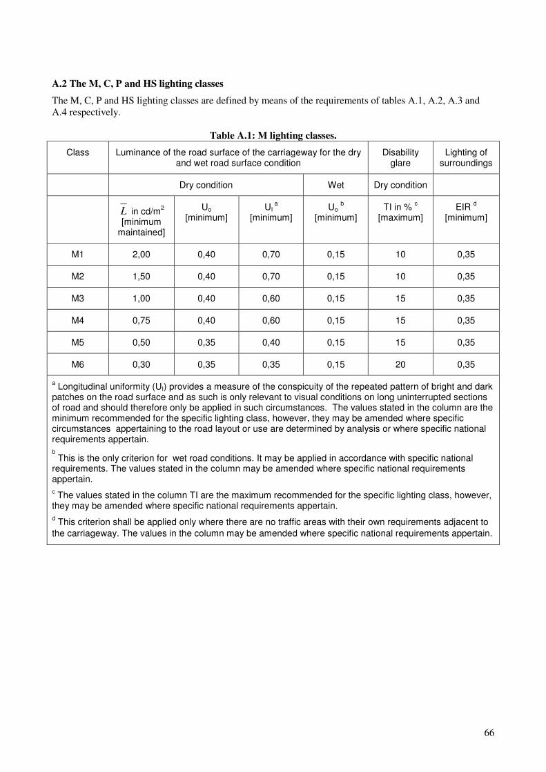
66

A.2 The M, C, P and HS lighting classes

The M, C, P and HS lighting classes are defined by means of the requirements of tables A.1, A.2, A.3 and

A.4 respectively.

Table A.1: M lighting classes.

Class Luminance of the road surface of the carriageway for the dry and wet road surface condition

Disability glare

Lighting of surroundings

Dry condition Wet Dry condition

L in cd/m2


Uo [minimum]

UI a

[minimum] Uo

b

[minimum] TI in %

c

[maximum] EIR

d

[minimum]

M1 2,00 0,40 0,70 0,15 10 0,35

M2 1,50 0,40 0,70 0,15 10 0,35

M3 1,00 0,40 0,60 0,15 15 0,35

M4 0,75 0,40 0,60 0,15 15 0,35

M5 0,50 0,35 0,40 0,15 15 0,35

M6 0,30 0,35 0,35 0,15 20 0,35

a Longitudinal uniformity (UI) provides a measure of the conspicuity of the repeated pattern of bright and dark

patches on the road surface and as such is only relevant to visual conditions on long uninterrupted sections of road and should therefore only be applied in such circumstances. The values stated in the column are the minimum recommended for the specific lighting class, however, they may be amended where specific circumstances appertaining to the road layout or use are determined by analysis or where specific national requirements appertain.

b

This is the only criterion for wet road conditions. It may be applied in accordance with specific national requirements. The values stated in the column may be amended where specific national requirements appertain.

c The values stated in the column TI are the maximum recommended for the specific lighting class, however,

they may be amended where specific national requirements appertain.

d This criterion shall be applied only where there are no traffic areas with their own requirements adjacent to

the carriageway. The values in the column may be amended where specific national requirements appertain.

67

Table A.2: C lighting classes.



Uo [minimum]

C0 50 0,40

C1 30 0,40

C2 20,0 0,40

C3 15,0 0,40

C4 10,0 0,40

C5 7,50 0,40

Table A.3: P lighting classes.


E in lx a

[minimum maintained] Emin in lx

[maintained]

P1 15,0 3,00

P2 10,0 2,00

P3 7,50 1,50

P4 5,00 1,00

P5 3,00 0,60

P6 2,00 0,40

P7 performance not determined performance not determined

a To provide for uniformity, the actual value of the maintained average

illuminance must not exceed 1,5 times the minimum E value indicated for the class.

Table A.4: HS lighting classes.

Class Hemispherical illuminance


U0 minimum]

HS1 5,00 0,15

HS2 2,50 0,15

HS3 1,00 0,15

HS4 performance not determined performance not determined

68

Depreciation of light output

0,0

0,2

0,4

0,6

0,8

1,0

1,2

0 20 40 60 80

Months

Facto

rs

factor for light source

factor for dirt on luminaire

factor for ageing of luminaire

product of factors

A.3 The maintenance factor

All types of electric light sources experience lumen depreciation, defined as the gradual decrease in light

output that occurs as a lamp is operated. An additional gradual depreciation of the light output is caused by

accumulation of dirt on the optical parts of the luminaires.

It is normally assumed that the light output is restored at intervals by maintenance involving replacement of

the light sources and cleaning of the optical parts of the luminaires. The restoration of the light output may

not be full, as ageing of the optical parts of the luminaires may cause irreversible loss of light.

EXAMPLE:

The figure illustrates the various factors

for depreciation of light output as a

function of time.

It is assumed that light sources are

replaced every 12 months and that the

optical parts of the luminaires are

replaced at the same time.

In lighting schemes this is normally described by a maintenance factor MF with a value less than one. The

value is applied as a reduction factor for the level of illumination in designs of lighting installations and is

selected in view of the light sources, the luminaires, the surrounds and the maintenance scheme to be carried

out.

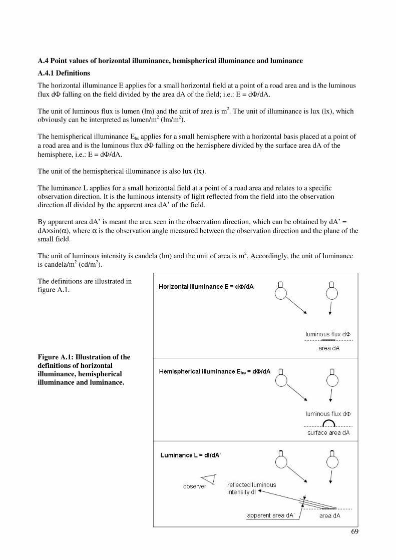
69

A.4 Point values of horizontal illuminance, hemispherical illuminance and luminance

A.4.1 Definitions

The horizontal illuminance E applies for a small horizontal field at a point of a road area and is the luminous

flux dΦ falling on the field divided by the area dA of the field; i.e.: E = dΦ/dA.

The unit of luminous flux is lumen (lm) and the unit of area is m2. The unit of illuminance is lux (lx), which

obviously can be interpreted as lumen/m2 (lm/m

2).

The hemispherical illuminance Ehs applies for a small hemisphere with a horizontal basis placed at a point of

a road area and is the luminous flux dΦ falling on the hemisphere divided by the surface area dA of the

hemisphere, i.e.: E = dΦ/dA.

The unit of the hemispherical illuminance is also lux (lx).

The luminance L applies for a small horizontal field at a point of a road area and relates to a specific

observation direction. It is the luminous intensity of light reflected from the field into the observation

direction dI divided by the apparent area dA’ of the field.

By apparent area dA’ is meant the area seen in the observation direction, which can be obtained by dA’ =

dA×sin(α), where α is the observation angle measured between the observation direction and the plane of the

small field.

The unit of luminous intensity is candela (lm) and the unit of area is m2. Accordingly, the unit of luminance

is candela/m2 (cd/m

2).

The definitions are illustrated in

figure A.1.

Figure A.1: Illustration of the

definitions of horizontal

illuminance, hemispherical

illuminance and luminance.

70

The horizontal illuminance E is a simple concept, being a measure of the density of light falling at a location

on a horizontal surface. The value has rotational symmetry in the sense that it does not matter if the light

comes from the side, front or the back or any other plane in between. This shows up also in the way that a

measured value in insensitive to rotation of the lux meter, as long as it is held horizontally.

The hemispherical illuminance Ehs is an equally simple concept. It has the same rotational symmetry as the

horizontal illuminance and differs only by having a different variation with the angle of incident light.

The luminance, on the other hand, has a more complex definition. Additionally, the value is a matter of not

only of illumination, but also of reflection in the surface.

Reflection is simple, when the surface has diffuse reflection. In this case, the luminance is derived by L =

ρ×E/π, where ρ is the reflectance of the surface and E is the horizontal illuminance. The division with π in

the conversion from illuminance to luminance is inherent in the definitions of illuminance and luminance.

Because of the division with π, and because the value of ρ is less than 1, the numerical value of the

luminance is smaller than the numerical value of the illuminance.

In road lighting, the reflection takes place in the road surface, which does not have diffuse reflection.

Because of this, the calculation of luminance is more complex than the calculation of illuminance, and the

result depends on the observation direction. This breaks the rotational symmetry that applies for illuminance.

The concept of luminance is more fundamental than the concept of illuminance in the sense that luminance is

the stimulus for vision. Luminance can be observed, while illuminance cannot – at least not directly.

Therefore, road lighting design based on luminance is more directly related to visual performance than road

lighting design based on illuminance. It is a simple point of view to think of the road surface luminance at a

location on the road as a blurred image of the luminous apertures of the luminaires above the location.

It is only in terms of the definition of luminance and calculations of luminance in road lighting that the

concept of luminance is the more complex. This, on the other hand, limits the use of luminance design to

roads where only a few observer positions need to be considered.

A.4.2 Equations for the calculation of point values

The lighting parameters discussed in A.4.1 - horizontal illuminance, hemispherical illuminance and

luminance - are additive in the sense that a value at a point is the sum of the contributions from the individual

luminaires of the lighting installation. Therefore, it is sufficient to consider the contribution from a single

luminaire at a time.

The contribution to the horizontal illuminance E at a point is calculated by means of the two laws of

illumination, the distance law and the cosine law:

dE(i) = I(i)×cos(v)/d2 (1)

where dE(i) means the contribution from luminaire number i

I(i) means the luminous intensity from luminaire number i in the direction towards the point

v is the angle of incidence

and d is the distance from the point to the luminaire.

This expression implies that the luminaire is treated as a point source with the point located in an optical

centre of the luminaire. This is permissible, when the luminous aperture of the luminaire is small compared

to its mounting height above the road area. That is mostly the case except for special cases such as use of

luminous columns or bands.

71

The angle of incidence v is measured from the vertical to the direction of illumination as shown in figure

A.2.

Figure A.2: The angle of incidence.

Figure A.3 shows the vertical plane that contains the point and the luminaire, and illustrates that the distance

d is linked to the mounting height of the luminaire h by h = d×cos(v). This provides a value of the distance

by d = h/cos(v). Accordingly, equation 1 can be converted to:

dE(i) = I(i)×cos3(v)/h

2 (2)

where h is the mounting height of the luminaire.

This equation is more practical than equation 1, because the mounting height h is known and is the same for

all luminaires of a lighting installations - or least for a row of luminaires. The distance d need not be

determined, while the value of cos(v) has to be determined in any case.

Figure A.3: Measures in the vertical plane

containing the point and the luminaire.

Equation 2 can be written as:

dE(i) = Fh×I(i) (3)

where Fh is a factor given by Fh = cos3(v)/h

2

This is interesting, because the same equation can be used for the contribution to the hemispherical

illuminance dEhr(i) when replacing Fh with:

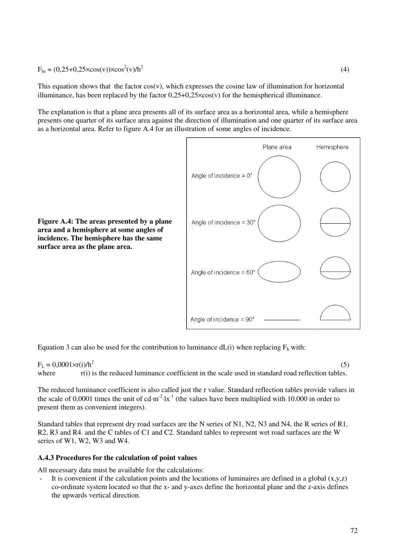
72

Fhs = (0,25+0,25×cos(v))×cos2(v)/h

2 (4)

This equation shows that the factor cos(v), which expresses the cosine law of illumination for horizontal

illuminance, has been replaced by the factor 0,25+0,25×cos(v) for the hemispherical illuminance.

The explanation is that a plane area presents all of its surface area as a horizontal area, while a hemisphere

presents one quarter of its surface area against the direction of illumination and one quarter of its surface area

as a horizontal area. Refer to figure A.4 for an illustration of some angles of incidence.

Figure A.4: The areas presented by a plane

area and a hemisphere at some angles of

incidence. The hemisphere has the same

surface area as the plane area.

Equation 3 can also be used for the contribution to luminance dL(i) when replacing Fh with:

FL = 0,0001×r(i)/h2 (5)

where r(i) is the reduced luminance coefficient in the scale used in standard road reflection tables.

The reduced luminance coefficient is also called just the r value. Standard reflection tables provide values in

the scale of 0,0001 times the unit of cd⋅m-2⋅lx-1 (the values have been multiplied with 10.000 in order to

present them as convenient integers).

Standard tables that represent dry road surfaces are the N series of N1, N2, N3 and N4, the R series of R1,

R2, R3 and R4. and the C tables of C1 and C2. Standard tables to represent wet road surfaces are the W

series of W1, W2, W3 and W4.

A.4.3 Procedures for the calculation of point values

All necessary data must be available for the calculations:

- It is convenient if the calculation points and the locations of luminaires are defined in a global (x,y,z)

co-ordinate system located so that the x- and y-axes define the horizontal plane and the z-axis defines

the upwards vertical direction.

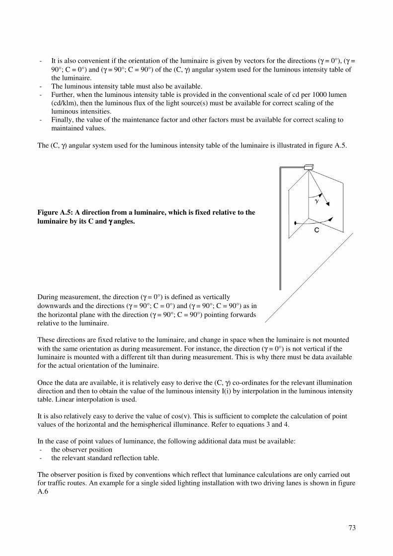
73

- It is also convenient if the orientation of the luminaire is given by vectors for the directions (γ = 0°), (γ =

90°; C = 0°) and (γ = 90°; C = 90°) of the (C, γ) angular system used for the luminous intensity table of

the luminaire.

- The luminous intensity table must also be available.

- Further, when the luminous intensity table is provided in the conventional scale of cd per 1000 lumen

(cd/klm), then the luminous flux of the light source(s) must be available for correct scaling of the

luminous intensities.

- Finally, the value of the maintenance factor and other factors must be available for correct scaling to

maintained values.

The (C, γ) angular system used for the luminous intensity table of the luminaire is illustrated in figure A.5.

Figure A.5: A direction from a luminaire, which is fixed relative to the

luminaire by its C and γγγγ angles.

During measurement, the direction (γ = 0°) is defined as vertically

downwards and the directions (γ = 90°; C = 0°) and (γ = 90°; C = 90°) as in

the horizontal plane with the direction (γ = 90°; C = 90°) pointing forwards

relative to the luminaire.

These directions are fixed relative to the luminaire, and change in space when the luminaire is not mounted

with the same orientation as during measurement. For instance, the direction (γ = 0°) is not vertical if the

luminaire is mounted with a different tilt than during measurement. This is why there must be data available

for the actual orientation of the luminaire.

Once the data are available, it is relatively easy to derive the (C, γ) co-ordinates for the relevant illumination

direction and then to obtain the value of the luminous intensity I(i) by interpolation in the luminous intensity

table. Linear interpolation is used.

It is also relatively easy to derive the value of cos(v). This is sufficient to complete the calculation of point

values of the horizontal and the hemispherical illuminance. Refer to equations 3 and 4.

In the case of point values of luminance, the following additional data must be available:

- the observer position

- the relevant standard reflection table.

The observer position is fixed by conventions which reflect that luminance calculations are only carried out

for traffic routes. An example for a single sided lighting installation with two driving lanes is shown in figure

A.6

74

Figure A.6: The observer position and a point within a field on the road area.

It is general within the conventions that the observer position is in the centre of a driving lane and 60 m in

front of a calculation field on the road, which stretches from one luminaire to the next. The observation

direction is the direction from the observer to the point within the field for which the calculations are done.

More details about the conventions will be provided later.

The r value is obtained by interpolation in the road reflection table, which has two entries, tan(v) and a side

angle β.

The angle v is the angle of incidence that is already described for the calculation of illuminance. Once the

value of cos(v) has been determined, it is relatively easy to determine tan(v).

The side angle β is measured between the projections of the observation and the illumination directions on

the road area. See figure A.7

It is also relatively easy to determine the value of β on the basis of the available data. The r value is then

determined by interpolation in the road reflection table. Linear interpolation is used.

Figure A.7: The side angle ββββ.

75

It may be noted that road reflection tables are measured with a constant observation angle α of 1°. With a

height of the observer above the road area of 1,5 m, this angle corresponds to a fixed distance of 86 m. The

actual distance from the observer to the points within the field may vary from approximately 60 m up to for

instance 100 m corresponding to a variation of α from 1,43° down to 0,86°.

This variation of the observation angle α is ignored in calculations of luminance by means of road reflection

tables. This is an approximation, but perhaps permissible because the r value does to a first approximation

not vary with the observation angle.

However, the variation of the height of observers above the road range in practise from perhaps 1,2 m for

drivers of passenger cars up to more than 2 m for drivers of large vehicles and this causes additional

variation of the observation angle. It has probably never been tested if the luminance really stays constant

within the practical range of α from perhaps 2° down to 0,5°.

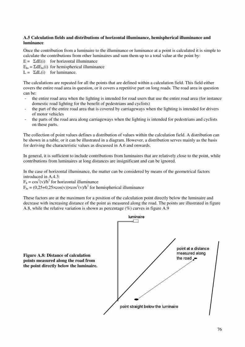
76

A.5 Calculation fields and distributions of horizontal illuminance, hemispherical illuminance and

luminance

Once the contribution from a luminaire to the illuminance or luminance at a point is calculated it is simple to

calculate the contributions from other luminaires and sum them up to a total value at the point by:

E = ΣdE(i) for horizontal illuminance

Ehs = ΣdEhs(i) for hemispherical illuminance

L = ΣdL(i) for luminance.

The calculations are repeated for all the points that are defined within a calculation field. This field either

covers the entire road area in question, or it covers a repetitive part on long roads. The road area in question

can be:

- the entire road area when the lighting is intended for road users that use the entire road area (for instance

domestic road lighting for the benefit of pedestrians and cyclists)

- the part of the entire road area that is covered by carriageways when the lighting is intended for drivers

of motor vehicles

- the parts of the road area along carriageways when the lighting is intended for pedestrians and cyclists

on these parts.

The collection of point values defines a distribution of values within the calculation field. A distribution can

be shown in a table, or it can be illustrated in a diagram. However, a distribution serves mainly as the basis

for deriving the characteristic values as discussed in A.6 and onwards.

In general, it is sufficient to include contributions from luminaires that are relatively close to the point, while

contributions from luminaires at long distances are insignificant and can be ignored.

In the case of horizontal illuminance, the matter can be considered by means of the geometrical factors

introduced in A.4.3:

Fh = cos3(v)/h

2 for horizontal illuminance

Fhr = (0,25+0,25×cos(v))×cos2(v)/h

2 for hemispherical illuminance

These factors are at the maximum for a position of the calculation point directly below the luminaire and

decrease with increasing distance of the point as measured along the road. The points are illustrated in figure

A.8, while the relative variation is shown as percentage (%) curves in figure A.9

Figure A.8: Distance of calculation

points measured along the road from

the point directly below the luminaire.

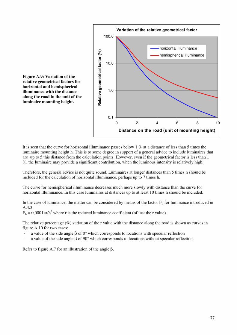
77

Figure A.9: Variation of the

relative geometrical factors for

horizontal and hemispherical

illuminance with the distance

along the road in the unit of the

luminaire mounting height.

It is seen that the curve for horizontal illuminance passes below 1 % at a distance of less than 5 times the

luminaire mounting height h. This is to some degree in support of a general advice to include luminaires that

are up to 5 this distance from the calculation points. However, even if the geometrical factor is less than 1

%, the luminaire may provide a significant contribution, when the luminous intensity is relatively high.

Therefore, the general advice is not quite sound. Luminaires at longer distances than 5 times h should be

included for the calculation of horizontal illuminance, perhaps up to 7 times h.

The curve for hemispherical illuminance decreases much more slowly with distance than the curve for

horizontal illuminance. In this case luminaires at distances up to at least 10 times h should be included.

In the case of luminance, the matter can be considered by means of the factor FL for luminance introduced in

A.4.3:

FL = 0,0001×r/h2 where r is the reduced luminance coefficient (of just the r value).

The relative percentage (%) variation of the r value with the distance along the road is shown as curves in

figure A.10 for two cases:

- a value of the side angle β of 0° which corresponds to locations with specular reflection

- a value of the side angle β of 90° which corresponds to locations without specular reflection.

Refer to figure A.7 for an illustration of the angle β.

Variation of the relative geometrical factor

0,1

1,0

10,0

100,0

0 2 4 6 8 10

Distance on the road (unit of mounting height)

Rela

tive g

eo

metr

ical

facto

r (%

) horizontal illuminance

hemispherical illuminance

78

Figure A.10: Variation of

the relative r value for

table N2 with the distance

along the road in the unit

of the luminaire mounting

height.

The curve for β = 90° is strongly similar to the curve for horizontal illumination shown in figure A.9. This

indicates that the road reflection is close to being of a diffuse nature for this value of β. This is actually the

case for most of the range of β.

The exception is a small range of β about 0°, where specular reflection causes much higher r values at large

distances. This is illustrated by the curve for β = 0° in figure A.9. It is noted that the curves are derived from

the standard table N2, which represents a low degree of specular reflection. Other tables of frequent use, like

R3, represent much higher degrees of specular reflection.

NOTE: There is an additional enhancement of r values for in a region of large values of the angle of incidence v with β

about 180°. This is due to coincidence of visible and illuminated facets.

Luminaires at large distances should be included, in particular in the forward direction. However, there is a

restriction which is set by the ranges of the angles γ and α that are covered by road reflection tables. This

restriction is expressed in terms of the luminaire mounting height h and is shown in figure A.11.

Variation of the relative r value (for table N2)

0,1

1,0

10,0

100,0

0 2 4 6 8 10 12

Distance on the road (unit of mounting height)

Rela

tive r

valu

e (

%)

beta = 0°

beta = 90°

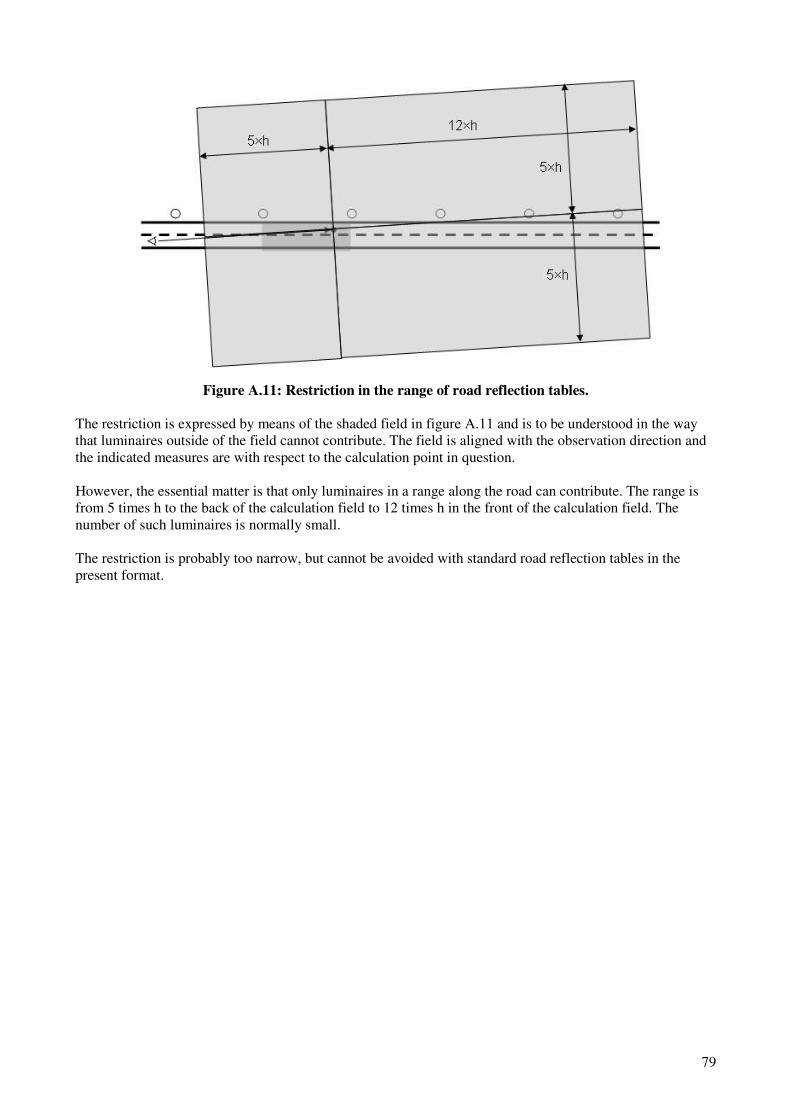
79

Figure A.11: Restriction in the range of road reflection tables.

The restriction is expressed by means of the shaded field in figure A.11 and is to be understood in the way

that luminaires outside of the field cannot contribute. The field is aligned with the observation direction and

the indicated measures are with respect to the calculation point in question.

However, the essential matter is that only luminaires in a range along the road can contribute. The range is

from 5 times h to the back of the calculation field to 12 times h in the front of the calculation field. The

number of such luminaires is normally small.

The restriction is probably too narrow, but cannot be avoided with standard road reflection tables in the

present format.

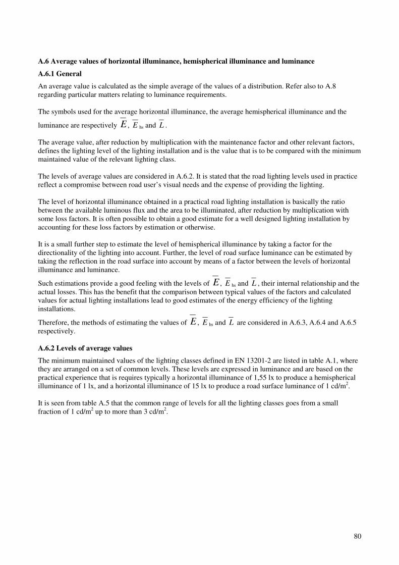
80

A.6 Average values of horizontal illuminance, hemispherical illuminance and luminance

A.6.1 General

An average value is calculated as the simple average of the values of a distribution. Refer also to A.8

regarding particular matters relating to luminance requirements.

The symbols used for the average horizontal illuminance, the average hemispherical illuminance and the

luminance are respectively E , E hs and L .

The average value, after reduction by multiplication with the maintenance factor and other relevant factors,

defines the lighting level of the lighting installation and is the value that is to be compared with the minimum

maintained value of the relevant lighting class.

The levels of average values are considered in A.6.2. It is stated that the road lighting levels used in practice

reflect a compromise between road user’s visual needs and the expense of providing the lighting.

The level of horizontal illuminance obtained in a practical road lighting installation is basically the ratio

between the available luminous flux and the area to be illuminated, after reduction by multiplication with

some loss factors. It is often possible to obtain a good estimate for a well designed lighting installation by

accounting for these loss factors by estimation or otherwise.

It is a small further step to estimate the level of hemispherical illuminance by taking a factor for the

directionality of the lighting into account. Further, the level of road surface luminance can be estimated by

taking the reflection in the road surface into account by means of a factor between the levels of horizontal

illuminance and luminance.

Such estimations provide a good feeling with the levels of E , E hs and L , their internal relationship and the

actual losses. This has the benefit that the comparison between typical values of the factors and calculated

values for actual lighting installations lead to good estimates of the energy efficiency of the lighting

installations.

Therefore, the methods of estimating the values of E , E hs and L are considered in A.6.3, A.6.4 and A.6.5

respectively.

A.6.2 Levels of average values

The minimum maintained values of the lighting classes defined in EN 13201-2 are listed in table A.1, where

they are arranged on a set of common levels. These levels are expressed in luminance and are based on the

practical experience that is requires typically a horizontal illuminance of 1,55 lx to produce a hemispherical

illuminance of 1 lx, and a horizontal illuminance of 15 lx to produce a road surface luminance of 1 cd/m2.

It is seen from table A.5 that the common range of levels for all the lighting classes goes from a small

fraction of 1 cd/m2 up to more than 3 cd/m

2.

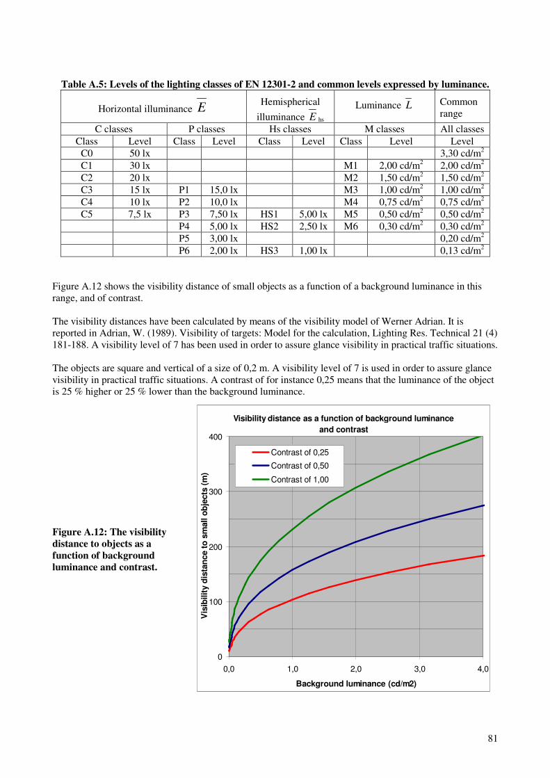
81

Visibility distance as a function of background luminance

and contrast

0

100

200

300

400

0,0 1,0 2,0 3,0 4,0

Background luminance (cd/m2)

Vis

ibilit

y d

ista

nce t

o s

mall o

bje

cts

(m

)

Contrast of 0,25

Contrast of 0,50

Contrast of 1,00

Table A.5: Levels of the lighting classes of EN 12301-2 and common levels expressed by luminance.

Horizontal illuminance E Hemispherical

illuminance E hs

Luminance L Common

range

C classes P classes Hs classes M classes All classes

Class Level Class Level Class Level Class Level Level

C0 50 lx 3,30 cd/m2

C1 30 lx M1 2,00 cd/m2 2,00 cd/m

2

C2 20 lx M2 1,50 cd/m2 1,50 cd/m

2

C3 15 lx P1 15,0 lx M3 1,00 cd/m2 1,00 cd/m

2

C4 10 lx P2 10,0 lx M4 0,75 cd/m2 0,75 cd/m

2

C5 7,5 lx P3 7,50 lx HS1 5,00 lx M5 0,50 cd/m2 0,50 cd/m

2

P4 5,00 lx HS2 2,50 lx M6 0,30 cd/m2 0,30 cd/m

2

P5 3,00 lx 0,20 cd/m2

P6 2,00 lx HS3 1,00 lx 0,13 cd/m2

Figure A.12 shows the visibility distance of small objects as a function of a background luminance in this

range, and of contrast.

The visibility distances have been calculated by means of the visibility model of Werner Adrian. It is

reported in Adrian, W. (1989). Visibility of targets: Model for the calculation, Lighting Res. Technical 21 (4)

181-188. A visibility level of 7 has been used in order to assure glance visibility in practical traffic situations.

The objects are square and vertical of a size of 0,2 m. A visibility level of 7 is used in order to assure glance

visibility in practical traffic situations. A contrast of for instance 0,25 means that the luminance of the object

is 25 % higher or 25 % lower than the background luminance.

Figure A.12: The visibility

distance to objects as a

function of background

luminance and contrast.

82

Visibility distance as a function of background luminance

and glare

0

25

50

75

100

0,0 0,3 0,5 0,8 1,0

Background luminance (cd/m2)

Vis

ibilit

y d

ista

nce t

o s

mall o

bje

cts

(m

)

No glare

Moderate glare (0,50 cd/m2)

Strong glare (1,00 cd/m2)

Small square objects may not be very relevant in traffic situation, and are used here just to illustrate that

conditions of visibility do improve with the level of lighting. Cases of low contrast should not be ignored

and, therefore, the lower of the curves in figure A.12 for a contrast of 0,25 needs to be taken into account.

This curve illustrates that road lighting levels reflect a compromise between the needs of road users and the

expense of providing the lighting.

The low end of the range represents road lighting for pedestrians and cyclists on for instance domestic roads.

The level can be low since fairly short visibility distances may be acceptable.

The high end of the range, on the other hand, represents road lighting for drivers in complex situations and

with a mixture of road users. Longer visibility distances need to be assured.

Figure A.13 shows the visibility distances for the object with a fairly low contrast of 0,25 in three situations;

without glare, with moderate glare and with strong glare.

The situation without glare is as for the previous figure A.12, which is also based on absence of glare. The

situations with glare are represented by veiling luminance values of 0,5 and 1 cd/m2. These levels correspond

to glare from the headlamps on oncoming vehicles – or just the level of ambient light as produced by other

lighting.

Figure A.13: The visibility

distance to objects as a

function of background

luminance and glare.

Figure A.13 shows that glare does lead to a reduction of the visibility distances. The reduction is significant

unless the background luminance is at least as high as the veiling luminance. This illustrates that the road

lighting should be able to compete with glare and ambient light.

83

The actual choice of road lighting levels for particular cases – as described in national standards or

regulations - is probably based on practical experience rather than deliberate investigations. Intuitive

understanding of the role of the background luminance and of glare has probably been a factor.

A.6.3 Simple estimation of the average horizontal illuminance

The average horizontal illuminance of a field is the ratio of the luminous flux falling on the field and the area

of the field.

NOTE: This is accurate only if the field is covered by calculation points with sufficiently small spacing, which is

normally the case.

This is useful for an estimation of the maximum value of the average horizontal illuminance that can be

provided by a lighting installation.

Assume that a field of an area A is illuminated by luminaires with a total installed luminous flux of the light

sources of Φ. The maximum possible value of E is then Φ/A. In some cases it is more easy to assign a

particular area A to each luminaire and then use the luminous flux Φ of the light source(s) of one luminaire

in the ratio Φ/A.

EXAMPLE 1: An 11 m wide road is illuminated by luminaires with a spacing of 35 m, each with a 50 W high pressure

sodium lamp with a luminous flux of 3500 lm. The maximum possible value of E is then 3500 lm/(11m×35 m) = 9

lm/m2 = 9 lx.

In the case of LED luminaires, it is often considered meaningless to measure the light output of the LED

light sources because it depends strongly on the supply and the conditions within the luminaire regarding

cooling. Therefore, a value of the light output of the light sources is often not available and in such cases the

maximum possible value of E has to be based of the light output from the luminaires instead.

The maximum possible value of E is not achieved in practice because of the following losses:

- depreciation of the light output

- loss of light in the luminaire

- loss of light outside of the road area to be illuminated.

Depreciation of the light output is accounted for by the value of the maintenance factor MF. This value is

often as low as 0,7.

Loss of light in the luminaire is traditionally described by an efficiency factor with a value of less than one.

The value is the ratio of the light output of the luminaire and the light output of the light source(s) of the

luminaire. The loss is caused by imperfections of the optical parts of the luminaires such as reflection losses

in mirror optics and transmission losses in screens at the luminaire aperture.

The light output of the light sources is measured in standard conditions involving use of a reference ballast,

an ambient temperature of 25°C and draft free air. The light output of the light sources may change when

mounted in a luminaire because of the actual conditions of supply and temperature within the luminaire.

Such changes are included in the efficiency factor.

The value of the efficiency factor is mostly fairly high, for instance 0,8.

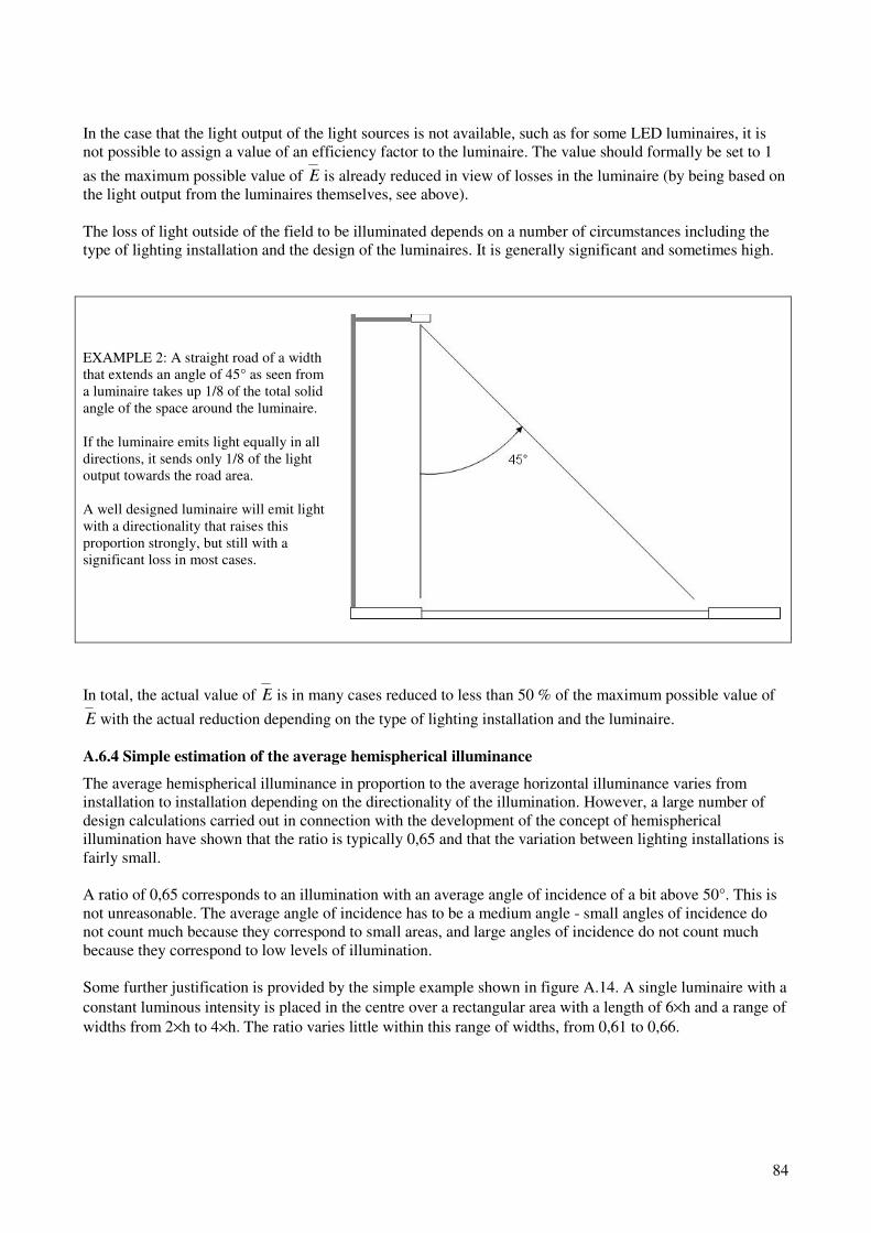
84

In the case that the light output of the light sources is not available, such as for some LED luminaires, it is

not possible to assign a value of an efficiency factor to the luminaire. The value should formally be set to 1

as the maximum possible value of E is already reduced in view of losses in the luminaire (by being based on

the light output from the luminaires themselves, see above).

The loss of light outside of the field to be illuminated depends on a number of circumstances including the

type of lighting installation and the design of the luminaires. It is generally significant and sometimes high.

EXAMPLE 2: A straight road of a width

that extends an angle of 45° as seen from

a luminaire takes up 1/8 of the total solid

angle of the space around the luminaire.

If the luminaire emits light equally in all

directions, it sends only 1/8 of the light

output towards the road area.

A well designed luminaire will emit light

with a directionality that raises this

proportion strongly, but still with a

significant loss in most cases.

In total, the actual value of E is in many cases reduced to less than 50 % of the maximum possible value of

E with the actual reduction depending on the type of lighting installation and the luminaire.

A.6.4 Simple estimation of the average hemispherical illuminance

The average hemispherical illuminance in proportion to the average horizontal illuminance varies from

installation to installation depending on the directionality of the illumination. However, a large number of

design calculations carried out in connection with the development of the concept of hemispherical

illumination have shown that the ratio is typically 0,65 and that the variation between lighting installations is

fairly small.

A ratio of 0,65 corresponds to an illumination with an average angle of incidence of a bit above 50°. This is

not unreasonable. The average angle of incidence has to be a medium angle - small angles of incidence do

not count much because they correspond to small areas, and large angles of incidence do not count much

because they correspond to low levels of illumination.

Some further justification is provided by the simple example shown in figure A.14. A single luminaire with a

constant luminous intensity is placed in the centre over a rectangular area with a length of 6×h and a range of

widths from 2×h to 4×h. The ratio varies little within this range of widths, from 0,61 to 0,66.

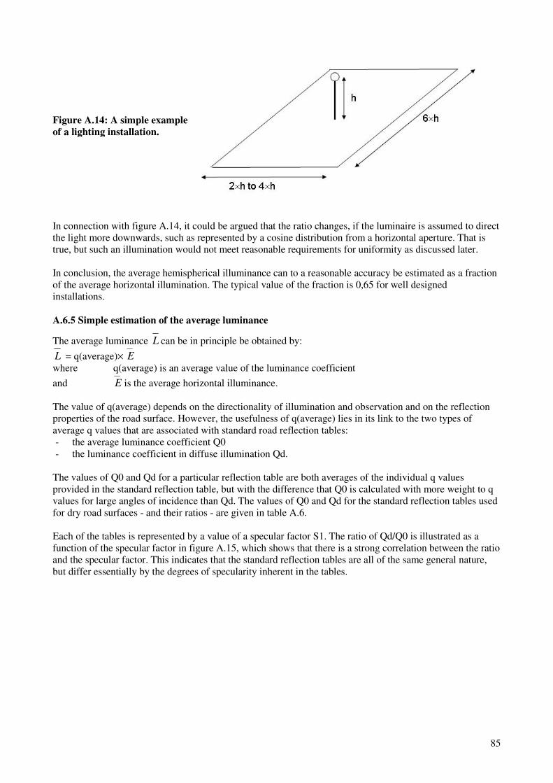
85

Figure A.14: A simple example

of a lighting installation.

In connection with figure A.14, it could be argued that the ratio changes, if the luminaire is assumed to direct

the light more downwards, such as represented by a cosine distribution from a horizontal aperture. That is

true, but such an illumination would not meet reasonable requirements for uniformity as discussed later.

In conclusion, the average hemispherical illuminance can to a reasonable accuracy be estimated as a fraction

of the average horizontal illumination. The typical value of the fraction is 0,65 for well designed

installations.

A.6.5 Simple estimation of the average luminance

The average luminance L can be in principle be obtained by:

L = q(average)× E

where q(average) is an average value of the luminance coefficient

and E is the average horizontal illuminance.

The value of q(average) depends on the directionality of illumination and observation and on the reflection

properties of the road surface. However, the usefulness of q(average) lies in its link to the two types of

average q values that are associated with standard road reflection tables:

- the average luminance coefficient Q0

- the luminance coefficient in diffuse illumination Qd.

The values of Q0 and Qd for a particular reflection table are both averages of the individual q values

provided in the standard reflection table, but with the difference that Q0 is calculated with more weight to q

values for large angles of incidence than Qd. The values of Q0 and Qd for the standard reflection tables used

for dry road surfaces - and their ratios - are given in table A.6.

Each of the tables is represented by a value of a specular factor S1. The ratio of Qd/Q0 is illustrated as a

function of the specular factor in figure A.15, which shows that there is a strong correlation between the ratio

and the specular factor. This indicates that the standard reflection tables are all of the same general nature,

but differ essentially by the degrees of specularity inherent in the tables.

86

Qd/Q0 as a function of the specular factor

0

0,2

0,4

0,6

0,8

1

0 0,5 1 1,5 2

Specular factor

Ra

tio

Qd

/Q0 N tables

R tables

C tables

Table A.6: Q0, Qd and their ratios for standard reflection tables for dry road surfaces.

Reflection

table

Q0

(cd⋅m-2⋅lx-1)

Qd

(cd⋅m-2⋅lx-1)

ratio Qd/Q0

N1

N2

N3 N4

0,100

0,070

0,070 0,080

0,092

0,061

0,054 0,054

0,92

0,87

0,78 0,68

R1

R2

R3 R4

0,100

0,070

0,070 0.080

0,087

0,057

0,050 0,052

0,87

0,81

0,71 0,65

C1

C2

0,100

0,070

0,090

0,054

0,90

0,77

Figure A.15: The ratio of Qd and Q0 as a function of the specular factor.

A large number of lighting installation design calculations that were carried out in connection with the

drafting of CIE 144 led to these findings:

- the value of q(average) is normally in between the values of Qd and Q0 for the standard reflection table

assumed in the individual design calculation

87

- the value of q(average) is closest to Q0, when the installation provides a relatively high degree of

illumination in specular directions, and closest to Qd, when the installation provides a relatively low

degree of illumination in specular directions.

The most common road lighting tradition prevailing in most of Europe leads to a relatively high degree of

illumination in specular directions and accordingly to q(average) values closest to Q0. Another road lighting

tradition, which is followed in a few countries only, leads to a reduction of the illumination in specular

direction and q(average) values closest to Qd.

These traditions are discussed elsewhere. In this connection it is stated only that it is in practice fairly

obvious if q(average) should be approximated by Q0 or Qd. In conclusion, the average luminance can to a

reasonable accuracy be estimated as a fraction of the average horizontal illumination. The fraction is either

Q0 or Qd.

The most common value to use for Q0 - almost the standard value - is 0,07 cd⋅m-2⋅lx-1. When reading the

standard values listed in table A.6, one should think that values for Qd should be lower. However, countries

abiding to the second road lighting tradition tend to use road surfaces with higher Qd values that those listed in

the table and, therefore, the value of 0,07 cd⋅m-2⋅lx-1 may be applied as the typical value in most cases.

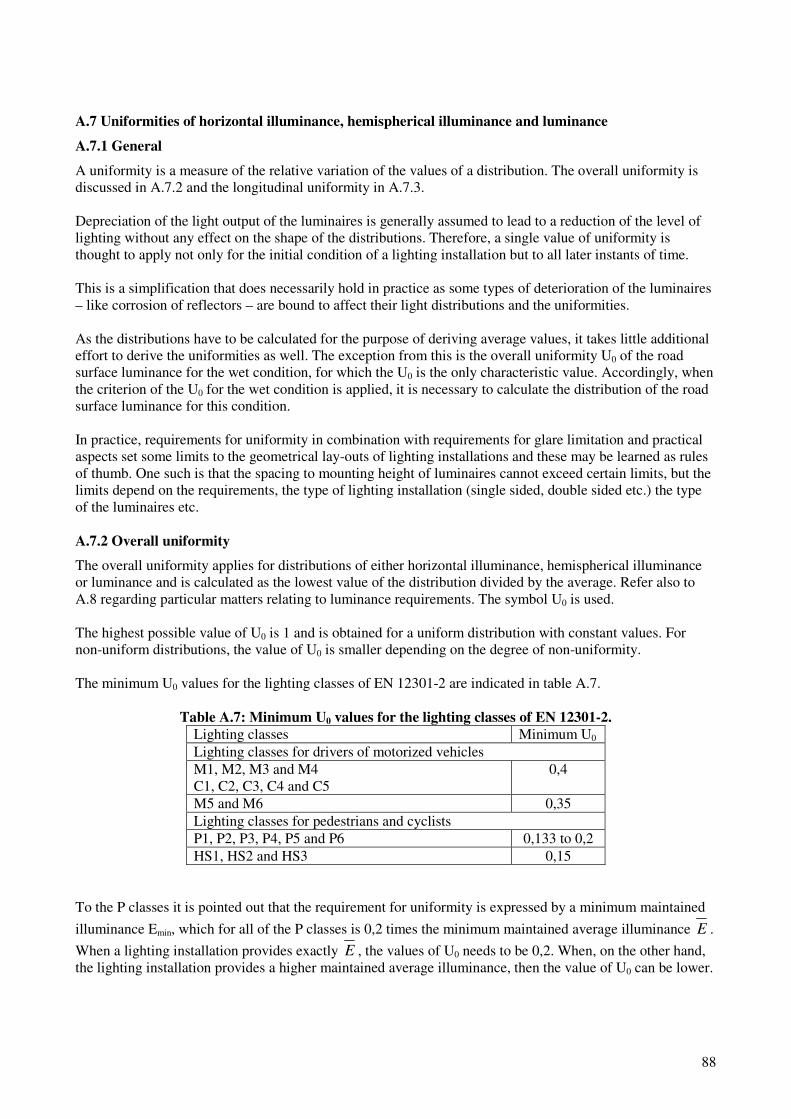
88

A.7 Uniformities of horizontal illuminance, hemispherical illuminance and luminance

A.7.1 General

A uniformity is a measure of the relative variation of the values of a distribution. The overall uniformity is

discussed in A.7.2 and the longitudinal uniformity in A.7.3.

Depreciation of the light output of the luminaires is generally assumed to lead to a reduction of the level of

lighting without any effect on the shape of the distributions. Therefore, a single value of uniformity is

thought to apply not only for the initial condition of a lighting installation but to all later instants of time.

This is a simplification that does necessarily hold in practice as some types of deterioration of the luminaires

– like corrosion of reflectors – are bound to affect their light distributions and the uniformities.

As the distributions have to be calculated for the purpose of deriving average values, it takes little additional

effort to derive the uniformities as well. The exception from this is the overall uniformity U0 of the road

surface luminance for the wet condition, for which the U0 is the only characteristic value. Accordingly, when

the criterion of the U0 for the wet condition is applied, it is necessary to calculate the distribution of the road

surface luminance for this condition.

In practice, requirements for uniformity in combination with requirements for glare limitation and practical

aspects set some limits to the geometrical lay-outs of lighting installations and these may be learned as rules

of thumb. One such is that the spacing to mounting height of luminaires cannot exceed certain limits, but the

limits depend on the requirements, the type of lighting installation (single sided, double sided etc.) the type

of the luminaires etc.

A.7.2 Overall uniformity

The overall uniformity applies for distributions of either horizontal illuminance, hemispherical illuminance

or luminance and is calculated as the lowest value of the distribution divided by the average. Refer also to

A.8 regarding particular matters relating to luminance requirements. The symbol U0 is used.

The highest possible value of U0 is 1 and is obtained for a uniform distribution with constant values. For

non-uniform distributions, the value of U0 is smaller depending on the degree of non-uniformity.

The minimum U0 values for the lighting classes of EN 12301-2 are indicated in table A.7.

Table A.7: Minimum U0 values for the lighting classes of EN 12301-2.

Lighting classes Minimum U0

Lighting classes for drivers of motorized vehicles

M1, M2, M3 and M4

C1, C2, C3, C4 and C5

0,4

M5 and M6 0,35

Lighting classes for pedestrians and cyclists

P1, P2, P3, P4, P5 and P6 0,133 to 0,2

HS1, HS2 and HS3 0,15

To the P classes it is pointed out that the requirement for uniformity is expressed by a minimum maintained

illuminance Emin, which for all of the P classes is 0,2 times the minimum maintained average illuminance E .

When a lighting installation provides exactly E , the values of U0 needs to be 0,2. When, on the other hand,

the lighting installation provides a higher maintained average illuminance, then the value of U0 can be lower.

89

However, it is a particular requirement that the actual value of the maintained average illuminance must not

exceed 1,5 times E and, therefore, the value of U0 cannot be lower than 0,2/1,5 = 0,133.

For the special case of U0 of the road surface luminance for the wet condition, the minimum requirement is

0,15. However, other requirements can be set in national requirements and indicated by the note b in table 1

for the M lighting classes of EN 13201-2:

“This is the only criterion for wet road conditions. It may be applied in accordance with specific national

requirements. The values stated in the column may be amended where specific national requirements

appertain”.

The intention of these requirements is to avoid that parts of the traffic area are very poorly illuminated. If, for

instance, the average horizontal illumination is 10 lx and the overall uniformity is 0,4 then the lowest

illuminance is 4 lx. As the highest illuminance may be for instance 20 lx in some locations, the illumination

may not appear to be quite uniform to the observer.

It can be noted that the requirements for U0 are relatively high for the lighting classes for drivers of

motorized vehicles, minimum 0,4 in most cases, while they are relatively low for the lighting classes for

pedestrians and cyclists, typically 0,15.

This does not necessarily reflect that pedestrians and cyclists have a lower need for uniformity than drivers

of motorized vehicles – rather that lighting installations with relatively low columns are preferred for

environmental reasons and that such lighting installation cannot provide high levels of uniformity.

A.7.3 Longitudinal uniformity

The longitudinal uniformity is applied only for distributions of road surface luminance and is calculated for

the values in the line of points with the same transverse location as the observer position as the lowest value

divided by the highest. Refer also to A.8 regarding particular matters relating to luminance requirements.

The symbol Ul is used.

The highest possible value of Ul is 1 and is obtained for a distribution with constant values in the line of

points. The value of Ul is less when the values vary.

The minimum requirements for Ul are provided in table 1 for the M lighting classes of EN 13201-2. They are

0,7 for M1 and M2, 0,6 for M3 and M4, 0,4 for M5 and 0,35 for M6. When taking into account that Ul is the

ratio between the lowest and the highest value, while U0 by comparison is the ratio between the lowest and

the average value, it can be understood that the requirements for Ul are quite high.

The intention of these requirements is make the road surface luminance in each driving lane appear uniform

so that the driver is not troubled by a repeated pattern of bright and dark patches on the road surface.

This is only relevant to visual conditions on long uninterrupted sections of road and should therefore only be

applied in relevant cases; for instance for the lighting of motorways. For this reason, the minimum

requirement for Ul can be set lower in national requirements. Refer to note a in table 1 for the M lighting

classes of EN 13201-2:

“Longitudinal uniformity (UI) provides a measure of the conspicuity of the repeated pattern of bright and

dark patches on the road surface and as such is only relevant to visual conditions on long uninterrupted

sections of road and should therefore only be applied in such circumstances. The values stated in the

column are the minimum recommended for the specific lighting class, however, they may be amended

where specific circumstances appertaining to the road layout or use are determined by analysis or where

specific national requirements appertain”.

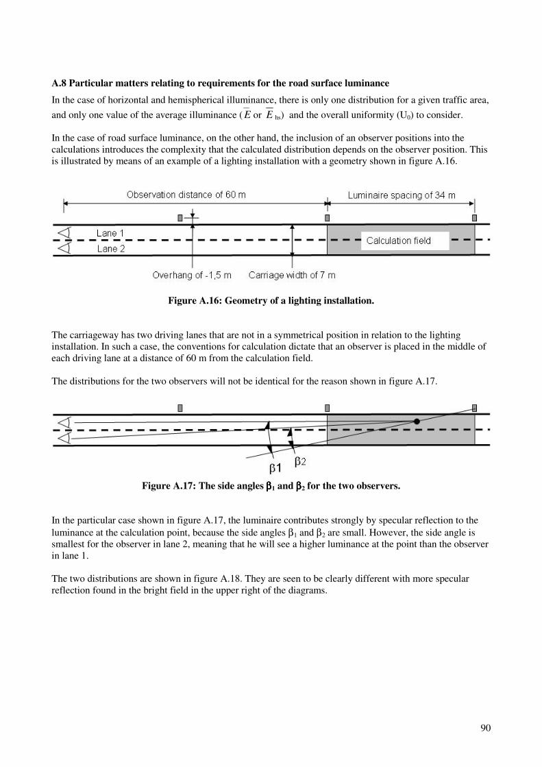
90

A.8 Particular matters relating to requirements for the road surface luminance

In the case of horizontal and hemispherical illuminance, there is only one distribution for a given traffic area,

and only one value of the average illuminance ( E or E hs) and the overall uniformity (U0) to consider.

In the case of road surface luminance, on the other hand, the inclusion of an observer positions into the

calculations introduces the complexity that the calculated distribution depends on the observer position. This

is illustrated by means of an example of a lighting installation with a geometry shown in figure A.16.

Figure A.16: Geometry of a lighting installation.

The carriageway has two driving lanes that are not in a symmetrical position in relation to the lighting

installation. In such a case, the conventions for calculation dictate that an observer is placed in the middle of

each driving lane at a distance of 60 m from the calculation field.

The distributions for the two observers will not be identical for the reason shown in figure A.17.

Figure A.17: The side angles ββββ1 and ββββ2 for the two observers.

In the particular case shown in figure A.17, the luminaire contributes strongly by specular reflection to the

luminance at the calculation point, because the side angles β1 and β2 are small. However, the side angle is

smallest for the observer in lane 2, meaning that he will see a higher luminance at the point than the observer

in lane 1.

The two distributions are shown in figure A.18. They are seen to be clearly different with more specular

reflection found in the bright field in the upper right of the diagrams.

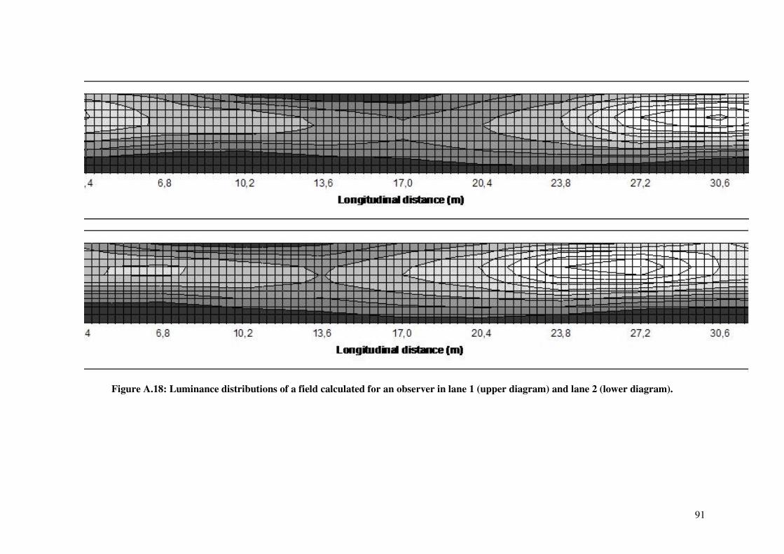
91

Figure A.18: Luminance distributions of a field calculated for an observer in lane 1 (upper diagram) and lane 2 (lower diagram).

The conventions dictate in general the use of one observer position in the middle of each driving lane, so that

the number of observer positions and distributions equals the number of driving lanes. However, in some

cases the two observer positions are in symmetrical positions with regard to both the road and the lighting

installation. In such cases, the two observer positions would provide identical or symmetrical distributions

with the same average value and uniformities, so that it is sufficient to include only one of them

Additionally, the conventions dictate that the lowest values of the average luminance L , as well as the

overall uniformity U0 and the longitudinal uniformity Ul for any of the observer positions are to be selected

to represent the lighting installation. The selected values L , U0 and Ul may result from different observer

positions.

Example: The lighting installation shown in figure A.18 results in these characteristic values:

Observer

position L (cd/m2) U0 Ul

In lane 1

In lane 2

0,58

0,62

0,44

0,42

0,44

0,70

Selected 0,58 0,42 0,44

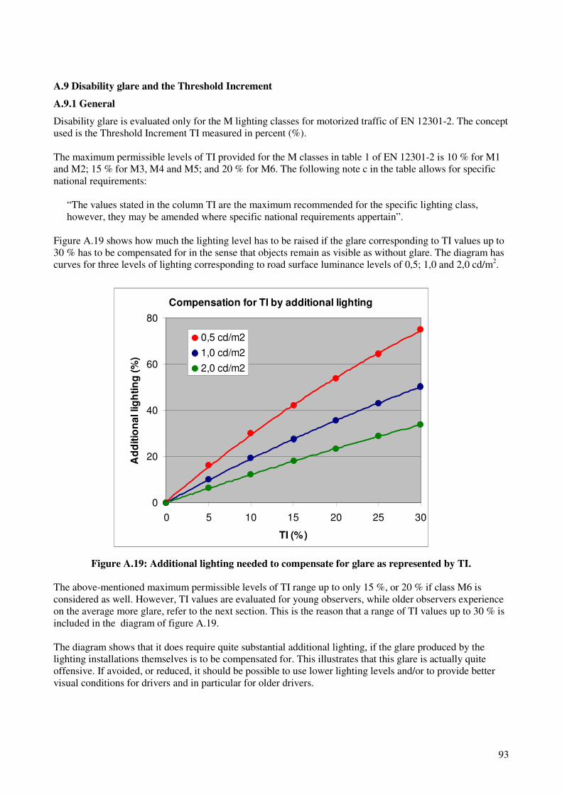
93

Compensation for TI by additional lighting

0

20

40

60

80

0 5 10 15 20 25 30

TI (%)

Ad

dit

ion

al lig

hti

ng

(%

)

0,5 cd/m2

1,0 cd/m2

2,0 cd/m2

A.9 Disability glare and the Threshold Increment

A.9.1 General

Disability glare is evaluated only for the M lighting classes for motorized traffic of EN 12301-2. The concept

used is the Threshold Increment TI measured in percent (%).

The maximum permissible levels of TI provided for the M classes in table 1 of EN 12301-2 is 10 % for M1

and M2; 15 % for M3, M4 and M5; and 20 % for M6. The following note c in the table allows for specific

national requirements:

“The values stated in the column TI are the maximum recommended for the specific lighting class,

however, they may be amended where specific national requirements appertain”.

Figure A.19 shows how much the lighting level has to be raised if the glare corresponding to TI values up to

30 % has to be compensated for in the sense that objects remain as visible as without glare. The diagram has

curves for three levels of lighting corresponding to road surface luminance levels of 0,5; 1,0 and 2,0 cd/m2.

Figure A.19: Additional lighting needed to compensate for glare as represented by TI.

The above-mentioned maximum permissible levels of TI range up to only 15 %, or 20 % if class M6 is

considered as well. However, TI values are evaluated for young observers, while older observers experience

on the average more glare, refer to the next section. This is the reason that a range of TI values up to 30 % is

included in the diagram of figure A.19.

The diagram shows that it does require quite substantial additional lighting, if the glare produced by the

lighting installations themselves is to be compensated for. This illustrates that this glare is actually quite

offensive. If avoided, or reduced, it should be possible to use lower lighting levels and/or to provide better

visual conditions for drivers and in particular for older drivers.

94

Methods and conventions for the calculation of TI are introduced in A.9.2, while the TI concept is discussed

in A.9.3.

It is pointed out that the methods and conventions lead to an “uncertainty” of calculations. This may go

deeper as an uncertainty regarding how a driver will be affected by the glare. Additionally, it is stated that

the concept of TI is complex and difficult to grasp.

In A.9.4, the use of luminaires of the full cut-off classes G*4, G*5 and G*6 for the purpose of glare control

is studied. It is concluded that luminaires of these classes can assure adequate glare control for the C lighting

classes and they are relevant for glare control for the M lighting classes as well.

A.9.2 Methods and conventions for the calculation of TI

As an intermediate step, the veiling luminance is calculated by the standard equation:

Lv = K×Σ(E/θ2)

Where Lv is the veiling luminance

K is a constant

Σ means summations over the luminaires of the lighting installation

E is the illuminance at the observer’s eyes from the luminaire measured in lux (lx)

And θ is the angle between the line of sight and the direction towards the luminaire measured in

degrees (°).

The equation represents scattering of light in the media of the eye. The constant K is given the value of 10,

which represents young observers. Older observers experience on the average more glare and should be

represented by higher values of K. This equation is provided in EN 13201-3:

+⋅=

4

4,66186,9

AK where A represents the age of the observer

The value of 10 is obtained for an age of 23 years, while twice that value is obtained for an age of 67 years.

The veiling luminance is obviously dependent on the location of the observer and his line of sight. These

matters are, therefore, described by conventions given in EN 12301-3:

a. the observers eyes are in the middle of a driving lane at a height of 1,5 m above the road

b. the line of sight is in a vertical plane parallel to the road and 1° downwards

c. luminaires at a distance of up to 500 m are included in the summation´

d. luminaires above a plane passing through the observers eyes and tilted 20° upwards are excluded from

the summation – this represents the limitation of the view by the roof of the vehicle.

Some of these conventions are illustrated in figure A.20.

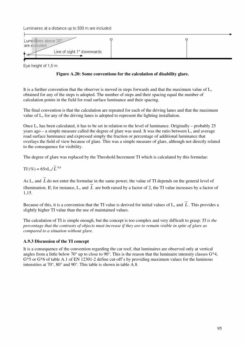
95

Figure A.20: Some conventions for the calculation of disability glare.

It is a further convention that the observer is moved in steps forwards and that the maximum value of Lv

obtained for any of the steps is adopted. The number of steps and their spacing equal the number of

calculation points in the field for road surface luminance and their spacing.

The final convention is that the calculation are repeated for each of the driving lanes and that the maximum

value of Lv for any of the driving lanes is adopted to represent the lighting installation.

Once Lv has been calculated, it has to be set in relation to the level of luminance. Originally – probably 25

years ago – a simple measure called the degree of glare was used. It was the ratio between Lv and average

road surface luminance and expressed simply the fraction or percentage of additional luminance that

overlays the field of view because of glare. This was a simple measure of glare, although not directly related

to the consequence for visibility.

The degree of glare was replaced by the Threshold Increment TI which is calculated by this formulae:

TI (%) = 65×Lv/ L 0,8

As Lv and L do not enter the formulae in the same power, the value of TI depends on the general level of

illumination. If, for instance, Lv and L are both raised by a factor of 2, the TI value increases by a factor of

1,15.

Because of this, it is a convention that the TI value is derived for initial values of Lv and L . This provides a

slightly higher TI value than the use of maintained values.

The calculation of TI is simple enough, but the concept is too complex and very difficult to grasp: TI is the

percentage that the contrasts of objects must increase if they are to remain visible in spite of glare as

compared to a situation without glare.

A.9.3 Discussion of the TI concept

It is a consequence of the convention regarding the car roof, that luminaires are observed only at vertical

angles from a little below 70° up to close to 90°. This is the reason that the luminaire intensity classes G*4,

G*5 or G*6 of table A.1 of EN 12301-2 define cut-off’s by providing maximum values for the luminous

intensities at 70°, 80° and 90°. This table is shown in table A.8.

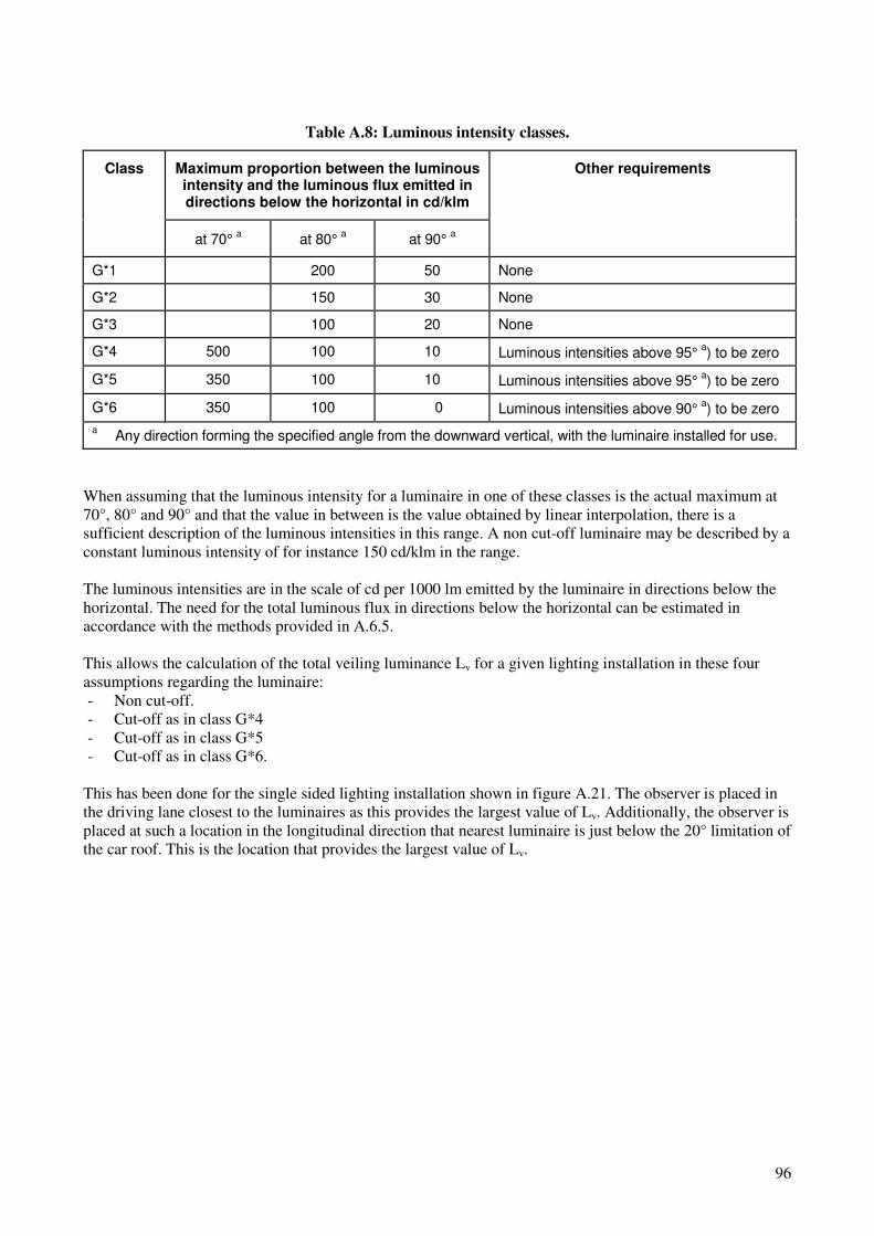
96

Table A.8: Luminous intensity classes.


Other requirements

at 70° a at 80°

a at 90°

a

G*1 200 50 None

G*2 150 30 None

G*3 100 20 None





When assuming that the luminous intensity for a luminaire in one of these classes is the actual maximum at

70°, 80° and 90° and that the value in between is the value obtained by linear interpolation, there is a

sufficient description of the luminous intensities in this range. A non cut-off luminaire may be described by a

constant luminous intensity of for instance 150 cd/klm in the range.

The luminous intensities are in the scale of cd per 1000 lm emitted by the luminaire in directions below the

horizontal. The need for the total luminous flux in directions below the horizontal can be estimated in

accordance with the methods provided in A.6.5.

This allows the calculation of the total veiling luminance Lv for a given lighting installation in these four

assumptions regarding the luminaire:

- Non cut-off.

- Cut-off as in class G*4

- Cut-off as in class G*5

- Cut-off as in class G*6.

This has been done for the single sided lighting installation shown in figure A.21. The observer is placed in

the driving lane closest to the luminaires as this provides the largest value of Lv. Additionally, the observer is

placed at such a location in the longitudinal direction that nearest luminaire is just below the 20° limitation of

the car roof. This is the location that provides the largest value of Lv.

97

Figure A.21: A single sided installation.

It is assumed that the initial emitted luminous flux in directions below the horizontal is 14.400 lm (14,4 klm)

and that 40 % of this luminous flux falls on the carriageway. This provides for an initial average illuminance

on the carriageway 17,8 lx and an initial value of the average luminance of 1,25 cd/m2, when assuming a Qd

value of 0,07.

The resulting summations of the veiling luminance for the four assumptions regarding the luminaire are

shown in figure A.22.

A feature to be noted from figure A.22 is that the sum of Lv keep increasing when adding contributions from

luminaires that are far away. This is in particular evident for the case of non cut-off luminaires, which is

discussed below.

This feature might be a surprise, considering that the contribution from a luminaire is in proportion to the

illuminance at the observers eyes and that this illuminance will decrease with the distance squared in

accordance with the distance law of illumination.

However, the contribution is also in inverse square proportion to the angle θ between the line of sight and the

direction to the luminaire. This angle decreases with distance as can be seen from figure A.23, and this

counteracts the distance law of illumination. The only reason that the contribution decreases with distance is

actually that the line of sight is 1° downwards. Had it been horizontal, the contributions from far away

luminaires would be constant and the sum would grow steadily without an upper limit.

98

Sums of veiling luminance for an increasing

number of luminaires

0,00

0,10

0,20

0,30

0,40

0,50

0,60

0,70

0 2 4 6 8 10 12 14 16 18 20

Number of luminaires

Su

m o

f veilin

g lu

min

an

ce

non cut-off

class G*4

class G*5

class G*6

500 m distance

Figure A.22: Sums of veiling luminance for an increasing number of luminaires.

Figure A.23: A single sided lighting installation seen in the perspective of the observer.

The above applies for the case of non cut-off luminaires. For the cases of cut-off luminaires, the contribution

an individual luminaire decreases more strongly with distance because of the decrease in luminous intensity.

However, it has to be concluded that disability glare measured by TI is high for installations with straight

rows of luminaires – because several of the luminaires in a row contribute to glare.

The 500 m distance, at which the summations are to be stopped in accordance with the conventions is also

indicated in figure A.22. The total Lv at this distance and the resulting TI values are indicated in table A.9.

99

TI variation with observer position for class G*6

0

4

8

12

16

1 2 3 4 5 6 7 8 9 10

Step of observer position

TI

valu

e (

%)

Table A.9: Lv and TI values.

Lv (cd/m2) TI (%)

Non cut-off

Cut-off as in class G*4



0,52

0,31

0,25

0,23

28,3

17,1

13,8

12,7

This table shows that the TI values decrease with stronger cut-off. However, some features of figure A.22

demonstrate that the matter is not very simple.

The first such feature is that the sum of Lv increases, when adding contributions from luminaires beyond the

500 m distance. This is in particular evident for the case of non cut-of , but even for the cases of cut-off there

is some increase.

This reflects a weakness of the conventions, as the 500 m distance has been set rather arbitrarily. If it had

been set longer or shorter, the TI values would change – in particular for the case of non cut-off.

Additionally, the matter that a luminaire may be just inside of just outside the 500 m distance introduces

some apparent random change of the TI value with small changes of the installation geometry.

The other feature is that the TI value has a discontinuous jump, when the observer is moved one step from a

position, where the nearest luminaire is just below the 20° plane representing the car roof, to the next

position along the road, where it is above.

This jump is large for luminaires with cut-off as illustrated for class G*6 in figure A.24. The explanation is

that the nearest luminaire contributes the most to the TI value, and that this contribution increases, when

approaching the luminaire – until the luminaire suddenly goes above the car roof.

Figure A.24: Variation of the TI value with the observer position for luminaires class G*6.

100

By convention the largest value of TI, in this case 15,2 %, is selected to represent the lighting installation. It

is a question if this is reasonable, as this level of glare occurs only in a short instant, when driving along the

road. An average value of 8,1 % might be more reasonable.

It is also a question, if the steps are arranged in such a way that the largest value of TI is actually found. If

the observer positions are moved just a bit ahead on the road, this would not be the case, and the next largest

value of 9,0 % would be selected to represent the lighting installation. This works like an uncertainty of

calculation where small changes of the installation geometry can cause large changes of the TI value.

In total, the TI concept used with the conventions described in the above is not good and needs to be

reworked.

A.9.4 Use of full cut-off luminaires

For lighting installations at conflict areas in accordance with the C classes of EN 13201-2 there are no clear

options for choosing the location and the direction of sight, or rather, there may be a multitude of options.

For this reason, table 2 of EN 13201-2 does not supply maximum TI values.

Instead, the informative annex A of prEN 13201-2 offers the advice that glare can be controlled by the use of

luminaires of the intensity classes G*.4, G*5, and G*6 defined in a table A.1 - refer to table A.8 of this

annex.

Additionally, because of the short-comings of the TI concept as discussed in A.9.3, it could be considered to

ensure additional glare control of lighting installations of the M classes for motorized traffic by the use of

luminaires of the above-mentioned classes.

The classes G*1, G*2 and G*3 correspond to "semi cut-off" and "cut-off" concepts of traditional use, with

requirements, however, modified to suit the prevailing use of light sources and luminaires. G*4, G*5 and

G*6 correspond to full cut-off.

As accounted for in A.9.3, the classes G*4, G*5 and G*6 provide restrictions for the luminous intensity at

the angles 70°, 80° and 90°, which are in the offending range for disability glare. The relevant directions are

generally not at precisely 70°, 80° and 90°, but it is reasonable to assume that actual luminaires in the classes

have luminous intensities at angles in between 70°, 80° and 90° that are limited by values derived by

interpolation.

Therefore, the classes G*4, G*5 and G*6 are considered for the control of disability glare in the following.

Figure A.25 illustrates a simple lighting installation for a rectangular conflict area with four luminaires

mounted at the corners of a rectangle.

101

Figure A.25: A simple lighting installation for a rectangular conflict area.

Calculations show that the TI values are low, less than 10 % and often much lower, as long as the input data

represent a reasonable geometry and a reasonably good use of the luminous output of the luminaires. This

applies for all of the three classes G*4, G*5 and G*6 with, however, the lowest TI values for the classes G*5

and G*6.

This shows that the use of full cut-off luminaires may provide glare control in such cases.

This conclusion is supported by the observation that the luminaires that contribute to glare also illuminate the

conflict area. This is opposed to the situation of lighting installations with rows of luminaires, where only a

few luminaires contribute to the illumination of the calculation field, while several of the luminaires

contribute to glare.

This can also be stated in a different manner; that the luminaires at a conflict area are not normally lined up

in a row parallel to an important line of sight.

The remaining question is then if the use of luminaires of the intensity classes G*.4, G*5, and G*6 will also

provide a useful control of glare for lighting installations of the M classes – where the luminaires do line up.

In order to supply an answer to this question, some estimated TI values are presented in figure A.26. The

estimations are carried out in the way accounted for in A.9.3 and for the single sided installation shown in

figure A.23 with an 8 m wide carriageway with two driving lanes and:

a. a value of the average maintained luminance L of 1 cd/m2

b. a value of the maintenance factor of 0,8

c. luminaires classified as G*6

d. a luminaire overhang of – 3 m

e. a luminaire mounting height in three steps of 8, 9 and 10 m

f. a luminaire spacing to mounting height ratio in three steps of 4,0; 4,5 and 5,0

g. a value of the utilisation factor of 0,5.

By utilization factor is meant the fraction of the installed luminous flux that falls in the carriageway.

102

Estimated TI values (%)

0

5

10

15

20

7 8 9 10 11

Luminaire mounting height (m)

TI

valu

e (

%)

spacing to height ratio of 5,0



Figure A.26: Estimated TI value for a single sided installation.

It is seen from figure A.26 that the TI value decreases somewhat with an increase of the mounting height and

increase somewhat with a decrease of the luminaire spacing to mounting height ratio. Apart from this, the TI

values are approximately 10 %.

This hints at some glare control, at least for luminaires of class G*6.

The TI value would tend to be lower for installations with more than one row of luminaires, and tend to be:

a. a bit lower/higher for lower/higher values of the average maintained luminance L than 1 cd/m2

b. a bit lower/higher for higher/lower values of the maintenance factor than 0,8

c. higher for luminaires classified lower than class G*6

d. a bit lower/higher for luminaires at longer/smaller distances from the road than given by an overhang of

– 3 m

e. lower/higher for values of the utilisation factor higher/lower than 0,5.

Additionally, the TI value is lower if the luminaires have luminous intensities that are lower than the

maximum values allowed for class G*6 at one or more of the angles 70°, 80° and 90° in those planes that

point towards the observer. It is likely that TI values are significantly lower in practical cases because of this.

The conclusion is that the use of luminaires of class G*6 and probably also classes G*4 and G*5 will ensure

a useful glare control in most cases.

103

A.10 Lighting of the surroundings of the carriageway

When lighting the carriageway for motorized traffic in accordance with the M classes of EN 13201-2, the

Edge Illumination Ratio, EIR may have to be considered.

The EIR is the average horizontal illuminance on a strip just outside the edge of a carriageway in proportion

to the average horizontal illuminance on a strip just inside the edge. The strips have the width of one driving

lane of the carriageway.

The requirement provided in table 1 of EN 12301-2 is that the EIR of both sides of the carriageway must be

minimum 0,35. However, a note d in the table states:

“This criterion shall be applied only where there are no traffic areas with their own requirements adjacent

to the carriageway. The values in the column may be amended where specific national requirements

appertain”.

Consequently, the EIR need not be applied if there are no traffic areas with their own requirements adjacent

to the carriageway. Further, the minimum value may be modified in national requirements.

The intention with the EIR requirement is to ensure that the lighting does not stop abruptly at the edges of

the carriageway as this causes a feeling like driving in a tunnel and also prevents visibility of road users or

animals about to enter the carriageway.

The requirement itself is weak. One of the driving lanes next to an edge may have a significantly lower

average ´horizontal illuminance than the carriageway as a whole, and the average horizontal illuminance

outside of the edge can drop to 25 % of that. Further, the uniformity of the illumination outside of the edge

may be poor as there is no requirement for that.

In total, it is allowed that parts of the strips outside of the carriageway are very poorly illuminated. This is

not desirable and not really necessary. The lighting installation with the luminance distributions shown in

figure A.18, is a quite common small single sided installation and, nevertheless, the EIR values of the two

edges are close to 0,50.

It is probably best to avoid the use of the EIR and always apply specific requirements to the areas outside of

the carriageway. After all, these areas mostly contain footways, cycle paths or parking areas. If not, the areas

may contain reserves or there may be road users on rare occasions.

The specific requirements should be formulated as requirements for pedestrians and cyclist by means of the

P or the HS lighting classes.

104

105

Annex B: Light sources for road lighting

B.1 Introduction and summary

Light and colour is introduced in B.2.


as described in a conventional manner.

The quantity of light is derived by a weighted summation of the radiation over the wavelengths followed by

multiplication of the sum with a standard factor. The weight factors reflect the relative variation of perceived

brightness with the wavelength λ, they are given by the V(λ) curve. The factor serves to provide lighting

units on the same scale as in older definitions of light, it has the value of 683 lumens per Watt (lm⋅W-1).

The characteristics used for lighting, as accounted for in annex X, are special versions of the characteristics

used for electromagnetic radiation. A comparison of characteristics, symbols and units used for

electromagnetic radiation and lighting is provided. The luminous efficacy of emitted light is the ratio

between the values of lighting and radiation characteristics, its value depends on the radiation spectrum.

The concepts behind the colour of emitted light reflect that:

- the human eye has three different kinds of photoreceptors with different variations of the sensitivity

with the wavelength of the electromagnetic radiation.




The colour of emitted light is represented by the chromaticity co-ordinates x and y, which define a point in

the CIE colour triangle. The colour temperature – or the correlated colour temperature – is a descriptive of

the colour of emitted light. Colour temperatures over 5000 K are called cool colours (bluish white), while

lower colour temperatures of 2700 to 3000 K are called warm colours (yellowish white through red).

Colour rendition of surface colours is measured by the colour rendering index Ra.

It is pointed out that light has the right photon energy to be useful for life by triggering chemical reactions of

organic compounds - including the pigments in the photoreceptors of the human eye and the chlorophyll

responsible for the photosynthesis of plants – and that the sun has the right temperature to produce an

abundance of light without an excess of ultraviolet radiation that causes damage organic compounds -

including DNA.

Production of light is introduced in B.3.

Humans have generated light and heat by fires and flames for a very long time. Excavations seem to indicate

that a predecessor of modern man, homo erectus could light and control fires. Lamps burning animal fat are

ancient and manmade lamps with wicks are older than the classic period of Greece. Olive oil, beeswax, fish

oil, whale oil, sesame oil, nut oil and other substances have been used as fuel. The petroleum lamp grew

popular 1800’s. Coal and natural gas lamps also became. Early in the 19th century, most cities in the United

States and Europe had streets that were gaslit.

A flame consists of vaporized molecules that react with oxygen in the air and produce transient reaction

intermediates with excited electrons that produce photons when returning to a lower energy state. It is clearly

a wasteful process as only a little of the energy is converted to light.

106

Any process – chemical or electrical - that changes the energy states of electrons involves photons and may

potentially result in the production of light. Therefore, light can be produced in many ways, but only the

following are described as relevant for road lighting:

- thermal radiation

- gas discharge

- fluorescence

- electroluminiscence.

Hot materials produce light by thermal radiation, which is electromagnetic radiation generated by the thermal

motion of charged particles in matter – in particular electrons. The perfect case is blackbody radiation that is

governed by some laws of physics. It is also the instructive case for other radiators, that emit less radiation

depending on the emissivity and the spectral distribution of the emissivity. The sun produces almost perfect

blackbody radiation, the filament of an incandescent lamp produces a little less than a blackbody at the same

temperature.

Thermal radiation is like cooking the atoms to provoke excitations of the electrons and results in a spectrum

that is much wider than the visible range. In spite of this, the sun produces light with a high luminous

efficacy of about 100 lm⋅W-1 because of its high surface temperature of approximately 6500 K. Incandescent

lamps have a much lower temperature of the filament and a much lower luminous efficacy because of

producing mainly infrared radiation.


discharge. This is like bombarding the atoms of the gas with electrons to provoke excitations of electrons of

the atoms and is obviously wasteful. It is a further matter that the spectrum of the emitted radiation depends

on the atoms of the gas and does not lend to production of light of a good quality in terms of colour of light

and colour rendition.

Electroluminiscence is the emission of light of a material in response to the passage of an electric current or

to a strong electric field. Light Emitting Diodes LED’s emits photons when passed by an electric current that

forces electrons and holes to recombine. This is an elegant way of converting electrical energy directly into

photon emission and the process with the highest potential for energy efficiency


radiation. Electrons in the substance are excited by the absorption of photons and release some of their

energy as photons. In most cases - and in general for light sources - the emitted light has a longer

wavelength, and therefore lower energy, than the absorbed radiation. This involves loss by its nature.



produced by fluorescence. Fluorescence is also used by white LED’s to convert blue light to other colours (a

white LED emits blue light but is embedded in a fluorescent layer).

Light sources are introduced in B.4.

The ideal light source for road lighting has a high luminous efficacy, a long useful life, a suitable light

output, a good quality of light (colour of light and colour rendition), small dimensions of the luminous parts

and can be dimmed.

The incandescent lamps were the first electrical lamps with wide application for road lighting and were a

major spur for the electrification of nations. They eventually failed in competition with other light sources

because of a poor luminous efficacy and a short useful life and are no longer used for road lighting. They are

actually being banned in general in many parts of the world.

107

It is peculiar that the gas discharge lamps used for road lighting can be divided into two broad families -

based on discharge in gases with either sodium or mercury as the main components.

In each of the two families there is a distinction between low pressure of the gas (low pressure sodium and

fluorescent lamps) and high pressure (high pressure sodium on one hand, and mercury and metal halide on

the other hand).


fluorescent lamps.



The gas discharge lamps were developed in this sequence:

Low-pressure sodium lamps

Mercury lamps and early versions of the fluorescent tubes


Compact fluorescent lamps

Metal halide CDM

Metal halide CPO

These lamps have competed with each other and supplemented each other for several decades as they entered

the market and were improved by developments.

The mercury lamps and early versions of the fluorescent tubes lived side by side for most lighting purposes

in a long period of time, being roughly equal in terms of lighting economy and quality of light. The mercury

lamps eventually got the upper hand because of the smaller size of the luminous parts that allowed better

optical control of the light and more freedom in the lay-out of lighting installations.

The high pressure sodium lamps replaced the mercury lamps in large road lighting installations and even

some of the small lighting installations because of a much better lighting economy – and in spite of a poor

quality of the light. The mercury lamps lived on in some of the small lighting installations, but are mow on

the way out – being banned in Europe.

The high pressure sodium lamps have kept their dominance for a long period of time, but are now in

competition with the metal halide lamps – in particular the CPO lamps. The CPO lamps match the high

pressure sodium lamps in terms of luminous efficacy, not quite in terms of useful life, but provide better

quality of light.

The more recent development of LED modules is a break through into a light source with good qualities in

all respects and a potential for further development. There might be a day, where the LED module is the only

light source for road lighting. Unless something else is invented – there are many ways to produce light.

108

B.2 Light and colour

B.2.1 Introduction to light and colour


as described in a conventional manner. Therefore, electromagnetic radiation and its spectral wavelength

distribution is introduced in B.2.2.

The band of wavelengths ranges formally from 360 nanometer to 830 nanometer, where a nanometer equals

10-9

m and is abbreviated to nm. Somewhat shorter ranges are often applied.

On this basis, visible light is introduced in B.2.3. The quantity of light is derived by a summation of the

radiation wavelength by wavelength using values of the so-called V(λ) curve as weighting factors. The sum

is converted to lighting units by multiplication with a standard factor of 683 lumens per Watt (lm⋅W-1).

The V(λ) curve reflects the relative variation of perceived brightness with the wavelength λ. Values of V(λ)

are found in tables in CIE publications. The factor serves to provide lighting units on the same scale as in

older definitions of light based on standard light sources.

It is explained that the characteristics used for lighting, as accounted for in annex X, are special versions of

the characteristics used for electromagnetic radiation. A comparison of characteristics, symbols and units

used for electromagnetic radiation and lighting is provided in table B.1.

Table B.1: Comparison of characteristics, symbols and units used for radiation and lighting.

Radiation Lighting Concept

Characteristic Symbol Unit Characteristic Symbol Unit

Total emission Radiated power P W Luminous flux Φ lm

Intensity in a direction Radiant intensity I W⋅sr-1

Luminous intensity I cd

Intensity on a surface Irradiance E W⋅m-2 Illuminance E lx

Intensity in a direction

from a surface

Radiance L W⋅sr-1⋅m-2

Luminance L cd⋅m-2

The ratio between values of lighting and radiation characteristic - called the luminous efficacy - is introduced

and it is explained that the value depends on the radiation spectrum. Actual values are accounted for in a few

cases in order to provide a basic understanding of the efficacies of practical light sources.

The concepts behind the colour of emitted light is introduced in B.2.4. The basis is that the human eye has

three different kinds of photoreceptors with different variations of the sensitivity with the wavelength of the

electromagnetic radiation. These sensitivities are represented by curves labelled x, y and z, where y is the

V(λ) curve and x and z are curves with peaks at respectively long and short wavelengths.

The curves x, y and z are used to provide weighted sums of the radiation spectrum called the tristimulus

values X, Y and Z. The Y value is converted to the relevant lighting characteristic, while the colour is

represented by the chromaticity co-ordinates x and y given by x = X/(X+Y+Z) and y = Y/(X+Y+Z). The

colour of light is normally indicated in the CIE colour triangle as a point with the x, y co-ordinates.

These concepts reflect that:




NOTE 1: This knowledge was made available by Isac Newton in 1672.

109

The colour temperature – or the correlated colour temperature – as a descriptive of the colour of emitted light

is introduced. The colour temperature is assigned by comparison to the colours of blackbody radiation whose

spectra are characterised by a temperature measured on the absolute temperature scale of Kelvin (K). Colour

temperatures over 5.000 K are called cool colours (bluish white), while lower colour temperatures of 2.700

to 3.000 K are called warm colours (yellowish white through red).

NOTE 2: The Kelvin temperature scale equals the Celcius temperature except that it has its zero point of the absolute

zero of -273 C.

NOTE 3: It is ironic that a cool and warm colours correspond to respectively high and low colour temperatures.

Colour rendition of surface colours - as measured by the colour rendering index Ra - is introduced in B.2.5. It

is estimated that the maximum efficacy of a light source with a high colour rendering index is 150 lm⋅W-1.

All of the above-mentioned colour conventions are those of the CIE x, y system. There are many other

systems in use for different applications, but those of the CIE x, y system are generally used for road lighting

applications.

All of the above is based on photopic vision, which is the vision of the eye under well-lit conditions. In

humans and many other animals, photopic vision allows colour perception, mediated by cone cells, and a

high visual acuity and temporal resolution.

NOTE 4: Scotopic vision is the vision of the eye under low light conditions at luminance levels of 10

−2 to 10

−6 cd⋅m2

.

This kind of vision can be disregarded because these luminance levels are too low to be relevant for road lighting.

NOTE 5: Mesopic vision is a combination of photopic vision and scotopic vision in low but not quite dark lighting

situations. In a period when light from Light Emitting Diodes (LED’s) was bluish, mesopic vision had some attention

because it would promote LED’s by comparison to other light sources. However, this attention has faded – probably

because LED’s were developed to compete with other light sources and because mesopic vision introduces some

difficulties of the conventions.

Light and colour is introduced in the above by means procedures involving summations over spectra and

other mathematical operations. Such procedures are actually employed, when using spectrophotometers for

the measurement of light and colour. However, it is most common to measure lighting characteristics in an

integral manner using photometers with a spectral sensitivity in accordance with the V(λ) curve.

Additionally, the tristimulus values X, Y and Z are sometimes measured in an integral manner using

photometers with spectral sensitivities in accordance with the x, y and z curves.

At this point it is stated that it is not a coincidence that vision occurs in the above-mentioned visible range of

wavelengths. The arguments are given in the following.

Electromagnetic radiation acts in packets called photons. These are elementary particles, the carriers of the

electromagnetic force and the agents in chemical processes. The energy of a photon is in inverse proportion

to the wavelength:

E = h×c/λ

where E is the energy of the photon

h is planks constant

c is the speed of light

and λ is the wavelength of the photon.

110

The energy is 2,48 electron Volts (eV) at 500 nm and 2 – 3 eV for photons in the visible range of

wavelengths. This is the energy needed to trigger chemical reactions of organic compounds including the

pigments in the photoreceptors of the human eye and the chlorophyll responsible for the photosynthesis of

plants.

NOTE 5: An electron Volt is the energy that it takes to move an electron 1 Volt against an electrical field. It is a

convenient measure for the energy exchanges in chemical reactions that are typically a few eV. As an example, it takes

4,09 eV to break one molecule of CO2 into one molecule of C and one molecule of O2.

Infrared light is found at longer wavelengths, where the photon energy is too low to cause chemical reactions

of organic compounds. Ultraviolet light is found at shorter wavelengths, where the photon energy high

enough to damage DNA and other organic compounds directly or indirectly by producing reactive oxygen.

The sun is a G type star of the right temperature to produce an abundance of light without excess ultraviolet

radiation – of which some is blocked by the ozone layer in the atmosphere. Additionally, the sun has a life

that is sufficient to allow development and evolution of life. Life as we know it is probably found only on

planets under stars like the sun. This is why there is no coincidence.

Photons are also the agents in electrical processes.

The working principle of the semiconductor photodiode is that visible photons are absorbed by electrons

which then have sufficient energy to pass in the reverse direction of the diode. This generates a current

through the circuit, in which the photodiode is inserted. By suitable amplification, spectral filtering and other

measures, photodiodes serve as photodetectors with very good properties such as virtual absence of a dark

signal, linearity, fast response, absence of hysteresis etc.

The working principle of a semiconductor Light Emitting Diode is the opposite of the photodiode. Electrons

are forced to pass in the reverse direction of the diode by a voltage. This brings the electrons into a state with

an additional energy that is released by the emission of photons.

B.2.2 Electromagnetic radiation and spectra

Light is electromagnetic radiation and is in family with other types of electromagnetic radiation like gamma

rays, X rays, UV (ultraviolet radiation), IR (infrared radiation), micro waves and etc. It is the wavelength that

distinguishes different kinds of electromagnetic radiation. The range of the wavelength is in principle

without limits, but within 10-16

m to 102 m for the above-mentioned types of radiation as illustrated in figure

B.1.

Figure B.1: Wavelengths of electromagnetic radiation.

A source of electromagnetic radiation may emit its radiation as lines at one or more wavelengths in a line

spectrum or as a continuous distribution over a range of wavelengths in a continuous spectrum. Radiation

spectra can also be in a mixture of the two types.

A spectrum can show the distribution any of these characteristics:

- P, radiant power measured in Watts (W)

111

The spectrum of irradiance by the sun

0,0

0,5

1,0

1,5

2,0

2,5

0 500 1000 1500 2000 2500 3000

Wavelength (nm)

Irra

dia

nc

e

- I, radiant intensity in a direction measured in Watts per steradian (W⋅sr-1

)

- E, irradiance on a surface measured in Watts per square metres (W⋅m-2)

- L, radiant intensity in a direction from a surface measured in Watts per steradian per square metres

(W⋅sr-1⋅m-2

).

In either of the cases, the values of the characteristic are presented in proportion to the unit used for the

wavelength.

As an example, the distribution of irradiance E by the sun at ground level is shown in figure B.2.

Figure B.2: Spectrum of irradiation by the sun.

The unit of irradiance is W⋅m-2 and the unit of wavelength used in the diagram of figure B.2 is nanometer

(nm) equal to 10-9

m. Accordingly, the scale of the irradiance used in the diagram is W⋅m-2⋅nm-1

.

The total irradiance can be obtained by summation of the irradiance over the spectrum - nanometer by

nanometer. For the diagram in figure B.2 the result is 1340 W⋅m-2.

NOTE: The spectrum in figure B.2 is provided in ASTM E-490 and applies in specific circumstances only. Other

spectra for sun irradiation may be found in the literature.

A spectrum is often provided in a relative manner, for instance so that the maximum value is 1. If so,

additional information is needed to provide absolute values – for instance the value of a scaling factor or the

absolute value of the sum.

B.2.3 Visible light

Electromagnetic radiation that gives the sensation of light to the human eye is often called visible light, even

if the word light in itself implies visible radiation.

However, visible light is provided by electromagnetic radiation in the narrow wavelength band about 0,5×10-

6 m that is indicated in figure B.3.

112

The V(lambda) curve

0,0

0,2

0,4

0,6

0,8

1,0

300 400 500 600 700 800

Wavelength (nm)

Re

lati

ve

va

lue

Figure B.3: The band of wavelengths in which electromagnetic radiation gives the sensation of light.

The sensitivity of the eye varies with the wavelength as given in a relative manner by the V(λ) curve shown

in figure B.4.

Figure B.4: The relative sensitivity of the eye as given by the V(λλλλ) curve.

Figure B.5 shows the V(λ) curve together with the sun spectrum of figure B.2, and also a curve for the

product of the two spectra nanometer by nanometer.

The sum of the product curve represents a weighted summation of the sun spectrum using the values of the

V(λ) curve as weight factors. Such a sum represents the sensation of brightness of the eye without scale. It is

converted to lighting units by multiplication with a standard factor of 683 lumens per Watt (lm⋅W-1).

The sum of the product curve in figure is an irradiance of 195 W⋅m-2. Multiplication with 683 lm⋅W-1

leads to

the result of 133.000 lm⋅m-2. This is to be understood as an illuminance in terms of lighting characteristics.

Further, the unit of lux (lx) equal to lm⋅m-2 is used in lighting so that the resulting illuminance by the sun at

ground level is 133.000 lx.

113

The V(lambda) curve, the sun spectrum and the

product

0,0

0,5

1,0

1,5

2,0

2,5

0 500 1000 1500 2000 2500 3000

Wavelength (nm)

Re

lati

ve

va

lue

V(lambda)

Sun

Product

Figure B.5: The V(λλλλ) curve, the sun spectrum and the product of the two.

This is how lighting characteristics are calculated on the basis of spectra. The unit of Watt (W) is replaced by

the unit of lumen (lm) and in some cases composite units are replaced by new units. The above-mentioned

replacement of lm⋅m-2 with lux (lx) is one case. A replacement of lm⋅sr

-1 with candela (cd) is another case.

NOTE 1: Such replacement of composite units with new units are known from other fields. An example is power

expressed in Watt instead of Joule per second.

The sum of the product curve in figure B.5 of 195 W⋅m-2 may be compared to the sum of the sun spectrum of

1340 W⋅m-2. This shows that the eye uses only a fraction of 195/1340 equal to 0,1446 of the energy of the

radiation of the sun. This fraction multiplied by the standard conversion value of 683 lm⋅W-1 results in a

value of 99 lm⋅W-1. This value is also obtained as the ratio of the illuminance and the irradiance of the sun at

ground level.

Such a value is called luminous efficacy. The maximum value is the value of 683 lm⋅W-1, which would be

obtained for radiation at a line at the wavelength of 555 nm, where the value of the V(λ) is 1. All other

spectra results in a lower luminous efficacy.

As an example of a potential for a high luminous efficacy, the spectrum of sodium vapour at low pressure

has, as shown in figure B.6, a strong emission at a line at approximately 589 nm and virtually no other

emission. This line corresponds to a value of V(λ) of 0,77 and a luminous efficacy of 525 lm⋅W-1.

This emission line is produced by low pressure sodium lamps, while lines that are broadened more or less are

produced by a range of high pressure sodium lamps.

NOTE 2: The sodium line consists actually of two lines very close to each other.

114

The V(lambda) curve and the sodium line

0,0

0,2

0,4

0,6

0,8

1,0

1,2

300 400 500 600 700 800

Wavelength (nm)

Re

lati

ve

va

lue

V(lambda)

Sodium line

The V(lambda) curve and standard illuminant A

0,0

0,2

0,4

0,6

0,8

1,0

1,2

0 500 1000 1500 2000 2500 3000

Wavelength (nm)

Re

lati

ve

va

lue

V(lambda)

Standard illuminant A

Figure B.6: The V(λλλλ) curve and the sodium line.

An example of a potentially low luminous efficacy is the spectrum of standard illuminant A as shown in

figure B.7. It obviously has a low degree of emission within the V(λ) curve and a luminous efficacy of only

18,8 lm⋅W-1. Standard illuminant A represents an incandescent tungsten filament lamp and has a spectrum in

accordance with blackbody radiation at a temperature of 2856 Kelvin (K).

Figure B.7: The V(λλλλ) curve and the spectrum of standard illuminant A.

In case of blackbody radiation, the potential luminous efficacy increases with the temperature to reach a

maximum at approximately the temperature of the sun of 6500 K.

The sun spectrum is represented by the spectrum of standard illuminant D65 in measurements. This spectrum

is in accordance with blackbody radiation at a temperature of 6500 K. The luminous efficacy is 111 lm⋅W-1.

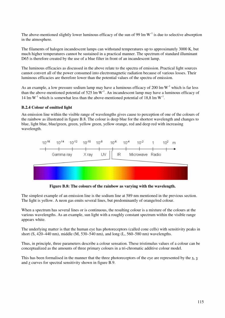
115

The above-mentioned slightly lower luminous efficacy of the sun of 99 lm⋅W-1 is due to selective absorption

in the atmosphere.

The filaments of halogen incandescent lamps can withstand temperatures up to approximately 3000 K, but

much higher temperatures cannot be sustained in a practical manner. The spectrum of standard illuminant

D65 is therefore created by the use of a blue filter in front of an incandescent lamp.

The luminous efficacies as discussed in the above relate to the spectra of emission. Practical light sources

cannot convert all of the power consumed into electromagnetic radiation because of various losses. Their

luminous efficacies are therefore lower than the potential values of the spectra of emission.

As an example, a low pressure sodium lamp may have a luminous efficacy of 200 lm⋅W-1 which is far less

than the above-mentioned potential of 525 lm⋅W-1. An incandescent lamp may have a luminous efficacy of

14 lm⋅W-1 which is somewhat less than the above-mentioned potential of 18,8 lm⋅W-1

.

B.2.4 Colour of emitted light

An emission line within the visible range of wavelengths gives cause to perception of one of the colours of

the rainbow as illustrated in figure B.8. The colour is deep blue for the shortest wavelength and changes to

blue, light blue, blue/green, green, yellow green, yellow orange, red and deep red with increasing

wavelength.

Figure B.8: The colours of the rainbow as varying with the wavelength.

The simplest example of an emission line is the sodium line at 589 nm mentioned in the previous section.

The light is yellow. A neon gas emits several lines, but predominantly of orange/red colour.

When a spectrum has several lines or is continuous, the resulting colour is a mixture of the colours at the

various wavelengths. As an example, sun light with a roughly constant spectrum within the visible range

appears white.

The underlying matter is that the human eye has photoreceptors (called cone cells) with sensitivity peaks in

short (S, 420–440 nm), middle (M, 530–540 nm), and long (L, 560–580 nm) wavelengths.

Thus, in principle, three parameters describe a colour sensation. These tristimulus values of a colour can be

conceptualized as the amounts of three primary colours in a tri-chromatic additive colour model.

This has been formalised in the manner that the three photoreceptors of the eye are represented by the x, y

and z curves for spectral sensitivity shown in figure B.9.

116

The x, y and z curves

0,0

0,5

1,0

1,5

2,0

350 400 450 500 550 600 650 700 750

Wavelength (nm)

Sp

ec

tra

l s

en

sit

ivit

y

x curve

y curve

z curve

Figure B.9: The x, y and z curves.

The x, y and z curves do not provide a true representation of the three photoreceptors of the human eye.

Instead, they have been constructed to be mathematically convenient while still accounting correctly for the

colour perception.

The y curve is actually the V(λ) curve used for summation of light as discussed in the previous section. The

x curve has its weight at long wavelengths corresponding to red light, while the z curve has its weight at

short wavelengths corresponding to blue light.

The curves are used for weighted summations of a spectrum in the manner accounted for in the previous

section for the V(λ) curve. The sums are the tristimulus values X, Y and Z.

The value of Y is the value of the relevant photometric characteristic, i.e.: luminous flux, luminous intensity,

illuminance or luminance. The values of X and Z are used to compute the chromaticity co-ordinates x and y

by means of:

x = X/(X+Y+Z)

y = Y/(X+Y+Z).

The values of x and y are used to indicate colours in the CIE 1931 colour space chromaticity diagram, also

called the CIE colour triangle, as shown in figure B.10.

Any colour of emitted light is represented by a point inside the colour space of the diagram. The points of

pure spectral colours lie along the curve limiting the colour space and are characterised by the wavelengths.

This curve is called the spectral locus. All other points are mixtures of pure spectral colours and lie inside the

spectral locus.

It might be noted that purple colours are mixtures of blue and red.

117

Figure B.10: The CIE colour triangle.

Blackbody radiation is characterized by a temperature measured in Kelvin (K) and their points in the CIE

colour triangle lie on a curve called the Planckian locus (Planckian because Max Planck explained the

spectra of blackbody radiation). Colour temperatures over 5.000 K are called cool colours (bluish white),

while lower colour temperatures of 2.700 to 3.000 K are called warm colours (yellowish white through red).

This is a convenient description of the colour of light. Additionally, most light sources emit light in spectra

that cover most or all of the visible range and are intended to resemble the spectra of blackbody radiation.

Therefore, most light sources are assigned a colour temperature.

This works easily and well for light sources whose chromaticity points lies on the Planckian locus or near to

it - for instance incandescent lamps.

Other light sources are instead assigned a correlated colour temperature, which is the temperature of the

blackbody radiation whose colour resembles best the colour of light of the light source. It requires more

mathematical operation to determine a correlated colour temperature, and it is not a perfect descriptive of the

actual colour of light.

Such light sources may for instance be high pressure sodium lamps, some of which are assigned a correlated

colour temperature as low as 1950 K. This, however, is a poor description of the colour of light.

The methods are not explained in detail, but the diagram in figure B.11 illustrates the concepts.

A light source needs to have a spectrum of emitted light that is similar to the spectrum of a blackbody

radiation, if it is to have a natural colour of light. The spectrum needs at least to cover some of the visible

range. This puts a limit to the luminous efficacy of emitted light and to the efficacy of the light source.

118

The spectral reflection of a red surface

0,0

0,2

0,4

0,6

0,8

1,0

300 400 500 600 700 800

Wavelength (nm)

Sp

ec

tra

l re

fle

cta

nc

e

Figure B.11: The Planckian locus (curve) and lines of correlated colour temperature.

B.2.5 Colour rendition of surface colours

The colour of a surface is neutral, when the spectral reflectance is constant within the visible wavelength,

and differs from neutral, when the spectral reflectance varies.

A neutral colour is described by its brightness and can be white, grey or black depending on the reflectance.

A non neutral colour needs a further description by for instance the type of colour and the saturation of the

colour. As an example, the spectral reflectance of a red surface is shown in figure B.12.

Figure B.12: Spectral reflectance of a red surface.

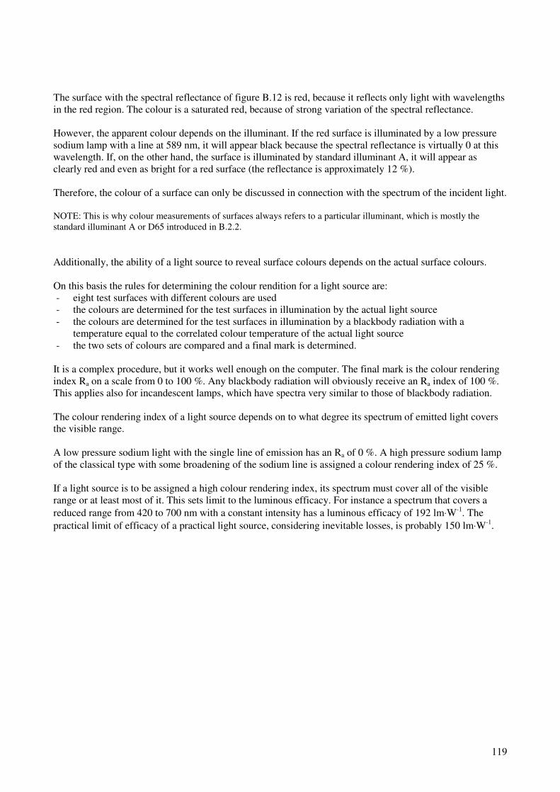
119

The surface with the spectral reflectance of figure B.12 is red, because it reflects only light with wavelengths

in the red region. The colour is a saturated red, because of strong variation of the spectral reflectance.

However, the apparent colour depends on the illuminant. If the red surface is illuminated by a low pressure

sodium lamp with a line at 589 nm, it will appear black because the spectral reflectance is virtually 0 at this

wavelength. If, on the other hand, the surface is illuminated by standard illuminant A, it will appear as

clearly red and even as bright for a red surface (the reflectance is approximately 12 %).

Therefore, the colour of a surface can only be discussed in connection with the spectrum of the incident light.

NOTE: This is why colour measurements of surfaces always refers to a particular illuminant, which is mostly the

standard illuminant A or D65 introduced in B.2.2.

Additionally, the ability of a light source to reveal surface colours depends on the actual surface colours.

On this basis the rules for determining the colour rendition for a light source are:

- eight test surfaces with different colours are used

- the colours are determined for the test surfaces in illumination by the actual light source

- the colours are determined for the test surfaces in illumination by a blackbody radiation with a

temperature equal to the correlated colour temperature of the actual light source

- the two sets of colours are compared and a final mark is determined.

It is a complex procedure, but it works well enough on the computer. The final mark is the colour rendering

index Ra on a scale from 0 to 100 %. Any blackbody radiation will obviously receive an Ra index of 100 %.

This applies also for incandescent lamps, which have spectra very similar to those of blackbody radiation.

The colour rendering index of a light source depends on to what degree its spectrum of emitted light covers

the visible range.

A low pressure sodium light with the single line of emission has an Ra of 0 %. A high pressure sodium lamp

of the classical type with some broadening of the sodium line is assigned a colour rendering index of 25 %.

If a light source is to be assigned a high colour rendering index, its spectrum must cover all of the visible

range or at least most of it. This sets limit to the luminous efficacy. For instance a spectrum that covers a

reduced range from 420 to 700 nm with a constant intensity has a luminous efficacy of 192 lm⋅W-1. The

practical limit of efficacy of a practical light source, considering inevitable losses, is probably 150 lm⋅W-1.

120

B.3 Production of light

B.3.1 Introduction to production of light

Humans have generated light and heat by burning for a very long time. Excavations seem to indicate that one

of our predecessors, homo erectus not only controlled fire but could light fires as long ago as perhaps one

million years.

The first lamp was invented around 70.000 BC. A hollow rock, shell or other natural found object was filled

with moss or a similar material that was soaked with animal fat and ignited. Humans began imitating the

natural shapes with manmade pottery, alabaster, and metal lamps. Wicks were later added to control the rate

of burning. Around the 7th century BC, the Greeks began making terra cotta lamps to replace handheld

torches. The word lamp is derived from the Greek word lampas, meaning torch.

Early lighting fuels consisted of olive oil, beeswax, fish oil, whale oil, sesame oil, nut oil, and similar

substances. When drilling for petroleum oil began mid 1800’s, the petroleum lamp grew popular. Coal and

natural gas lamps were also becoming wide-spread. Early in the 19th century, most cities in the United States

and Europe had streets that were gaslit.

Once a flame is ignited, the applied heat causes the fuel molecules to vaporize. In this state they can then

readily react with oxygen in the air, which gives off enough heat to vaporize yet more fuel, thus sustaining a

flame. Sufficient energy in the flame excites the electrons in some of the transient reaction intermediates,

which results in the emission of visible light.

Light production by burning is not considered further as burning is no longer used for road lighting.

Incandescent lamps produce light by thermal radiation, which is electromagnetic radiation generated by the

thermal motion of charged particles in matter – in particular electrons

Thermal radiation is considered in B.3.2. The starting point is blackbody radiation that is governed by some

laws of physics and instructive regarding light emission by other hot matter.


discharge. A discharge is sustained by an electrical field, which accelerates free electrons and cause them to

collide with the gas atoms. Some electrons in the atomic orbitals of these atoms are excited by these

collisions to a higher energy state. When an excited electron falls back to a lower energy state, it emits a

photon of a characteristic energy. Gas-discharge is considered in B.3.3.

Light Emitting Diodes LED’s generate light by electroluminiscence, in which a material emits light in

response to the passage of an electric current or to a strong electric field. Electroluminescence is the result of

recombination of electrons and holes in a material, usually a semiconductor. The electrons release the energy

they gain in recombination as photons.

This effect is explained in B.3.4 in view of LED’s. Other types of electroluminiscence – for instance in

panels used for backlighting – are not used for road lighting.

Some lamps - including gas-discharge lamps and white LED’s - use fluorescence to produce light or to

supplement the light emitted by other means.


radiation. In most cases - and in general for light sources - the emitted light has a longer wavelength, and

therefore lower energy, than the absorbed radiation. The process is that electrons in the substance are excited

by the absorption of photons and release some of their energy as photons. Fluorescence is considered in

B.3.5.

121

Any change of energy of an electron is by means of the electromagnetic force and photons are the carriers of

the electromagnetic force. Therefore, any process that changes the energy states of electrons involves

photons and may potentially result in the production of light. It is only a question of the wavelengths of the

photons and their possibility of escape.

Therefore, light can be produced in many ways, but only those that are useful for road lighting are mentioned

in the above. These processes are more or less wasteful:

- very little of the energy produced by burning results in light

- thermal radiation is like cooking the atoms to provoke excitations of the electrons and results in a

spectrum that is much wider than the visible range – and placed mainly outside of this range in the case

of incandescent lamps

- gas-discharge is like bombarding the atoms of the gas with electrons to provoke excitations of electrons

- electroluminiscence is an elegant way of converting electrical energy directly into photon emission and

the process with the highest potential for energy efficiency

- fluorescence involves loss by its nature of exchanging a photon with another photon of lower energy.

B.3.2 Thermal radiation

All matter emits electromagnetic radiation when it has a temperature above absolute zero. The radiation

represents a conversion of a body's thermal energy into electromagnetic energy, and is therefore called

thermal radiation.

The radiation of a completely black body can provide an insight into thermal radiation. The following laws

apply:

d. Stefan–Boltzmann law

e. Wien's displacement law

f. Planck's law

Stefan–Boltzmann law states that the radiance of a blackbody is in proportion to the absolute temperature to

the power of 4. The value of the factor is 5.67×10−8

W⋅m−2⋅K−4

Wien's displacement law states that the wavelength at which the radiation is at a maximum is in inverse

proportion to the absolute temperature. The value of the factor is 0,0029 K.

Planck's law provides a complete, but fairly complex formula for the spectral distribution.

The sun represents a good approximation to a black body with a temperature of 6500 K. The radiance is

approximately 1,0×108 W⋅m−2

and has its maximum at a wavelength of 446 nm, which is inside the visible

range. The luminance is approximately 100×108 cd⋅m-2

. At the ground surface, it has to be taken into account

that a bit of the radiation is lost in the atmosphere. However, the values explain the intensity of irradiation

and illumination by the sun, even at its huge distance from the earth.

A filament in an incandescent lamp is a less good approximation to a black body and radiates somewhat less

than a blackbody at the same temperature. Nevertheless, the main features can be derived by comparison to

blackbody radiation. An essential feature is the influence of the absolute temperature on the luminous

efficacy shown in figure B.13.

Figure B.13 shows that the luminous efficacy of an incandescent lamp increases strongly with the

temperature of the filament. Unfortunately the temperature cannot just be raised by increasing the current

through the filament as this results in a very strong reduction of the life of the filament. The filament

temperature used in modern standard lamps is in the range of 2800 to 2900 K.

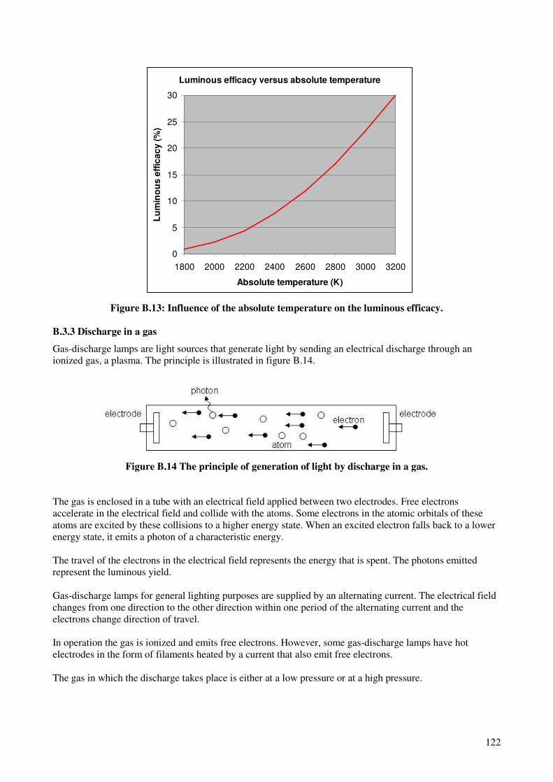
122

Luminous efficacy versus absolute temperature

0

5

10

15

20

25

30

1800 2000 2200 2400 2600 2800 3000 3200

Absolute temperature (K)

Lu

min

ou

s e

ffic

ac

y (

%)

Figure B.13: Influence of the absolute temperature on the luminous efficacy.

B.3.3 Discharge in a gas

Gas-discharge lamps are light sources that generate light by sending an electrical discharge through an

ionized gas, a plasma. The principle is illustrated in figure B.14.

Figure B.14 The principle of generation of light by discharge in a gas.

The gas is enclosed in a tube with an electrical field applied between two electrodes. Free electrons

accelerate in the electrical field and collide with the atoms. Some electrons in the atomic orbitals of these

atoms are excited by these collisions to a higher energy state. When an excited electron falls back to a lower

energy state, it emits a photon of a characteristic energy.

The travel of the electrons in the electrical field represents the energy that is spent. The photons emitted

represent the luminous yield.

Gas-discharge lamps for general lighting purposes are supplied by an alternating current. The electrical field

changes from one direction to the other direction within one period of the alternating current and the

electrons change direction of travel.

In operation the gas is ionized and emits free electrons. However, some gas-discharge lamps have hot

electrodes in the form of filaments heated by a current that also emit free electrons.

The gas in which the discharge takes place is either at a low pressure or at a high pressure.

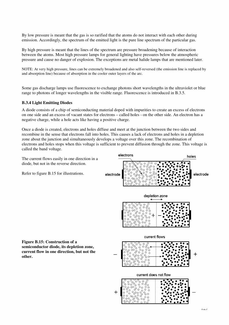
123

By low pressure is meant that the gas is so rarified that the atoms do not interact with each other during

emission. Accordingly, the spectrum of the emitted light is the pure line spectrum of the particular gas.

By high pressure is meant that the lines of the spectrum are pressure broadening because of interaction

between the atoms. Most high pressure lamps for general lighting have pressures below the atmospheric

pressure and cause no danger of explosion. The exceptions are metal halide lamps that are mentioned later.

NOTE: At very high pressure, lines can be extremely broadened and also self-reversed (the emission line is replaced by

and absorption line) because of absorption in the cooler outer layers of the arc.

Some gas discharge lamps use fluorescence to exchange photons short wavelengths in the ultraviolet or blue

range to photons of longer wavelengths in the visible range. Fluorescence is introduced in B.3.5.

B.3.4 Light Emitting Diodes

A diode consists of a chip of semiconducting material doped with impurities to create an excess of electrons

on one side and an excess of vacant states for electrons – called holes - on the other side. An electron has a

negative charge, while a hole acts like having a positive charge.

Once a diode is created, electrons and holes diffuse and meet at the junction between the two sides and

recombine in the sense that electrons fall into holes. This causes a lack of electrons and holes in a depletion

zone about the junction and simultaneously develops a voltage over this zone. The recombination of

electrons and holes stops when this voltage is sufficient to prevent diffusion through the zone. This voltage is

called the band voltage.

The current flows easily in one direction in a

diode, but not in the reverse direction.

Refer to figure B.15 for illustrations.

Figure B.15: Construction of a

semiconductor diode, its depletion zone,

current flow in one direction, but not the

other.

124

However, the current does flow in the reverse direction if the voltage applied over the electrodes of the diode

equals the band gap voltage and thereby force electrons and holes to meet and recombine. In this process, an

electron receives an energy equal to the charge of the electron multiplied with the band gap voltage, which it

discharges as a photon with the same energy.

This principle works for all diodes, but the particular matters of light emitting diodes (LED’s) are that the

generated photons have wavelengths in the visible range and that the construction of the diodes allows the

photons, or most of the photons, to escape.

The energy of a emitted photon E is reflected by the wavelength of the photon by λ= 1240 nm⋅eV/E eV,

where λ is the wavelength in nm. As an example, a band voltage of 2,48 V results in an energy of 2,48 eV of

the photon and a wavelength of 500 nm.

As the band voltage is characteristic of the semiconducting materials of the diode, a particular kind of LED

emits photons of a particular energy and thereby wavelength and colour.

It has been a substantial research and development work to arrive at different materials that produce light at

wavelengths ranging from the infrared over the colours of the visible spectrum to ultraviolet. Part of the

work has been to find materials and designs that allows the majority of the photons to escape the diode and

to create LED’s that can withstand a significant power without being destroyed the heating effects of the

current.

Over a period extending more than 30 years, the maximum luminous output of LED’s has been raised from

0,001 lm to now approaching 100 lm.

LED’s of the various signal colours like red, green and yellow have become the dominating light sources for

a large variety of signal lights.

However, white light is needed for lighting purposes. White light can in principle be composed of the light

from LED’s with different colours of emitted light like red, green and blue, but the development has taken

the way of using blue light in combination with fluorescence to produce white light. Fluorescence is

introduced in the next section.

The available luminous flux per LED is sufficient for signal lights, but still small in view of the needs of road

lighting of perhaps 2 000 to 150 000 lm per light point. The development has gone in the direction of

combining a fairly large number of LED’s in modules, that do meet this need.

B.3.5 Fluorescence

Fluorescence is the absorption of a photon of a certain wavelength in exchange for emission of a photon of a

longer wavelength.

Fluorescence is used by fluorescent tubes that work by discharge in a mercury gas at a low pressure. The

emission lines are at 184 nm and 253 nm in the UV-C region – potentially dangerous and not visible to the

human eye. However, a fluorescent coating on the inside of the tube prevents escape of the UV-C photons

and exchanges most of them with photons at longer wavelengths in the visible range. This principle is

illustrated in figure B.16.

125

Figure B.16: The principle of fluorescence in fluorescent tube.

Fluorescence is also used by mercury lamps to produce red light as a supplement to the green and violet light

emitted by the discharge. The fluorescence takes place in a coating on the inside of an exterior bulb.

Additionally, fluorescence is used by white LED’s. The light emitting diode of a white LED actually

produces blue light, but it is embedded in a fluorescent layer that exchanges a part of the blue light for light

at longer wavelengths.

Fluorescence involves a loss of energy, as the energy of a photon of a given wavelength is traded for a

photon of a longer wavelength and thereby a lower energy.

In the case of fluorescent tubes the loss is big because 184 nm and 253 nm photons are traded for photons in

the visible range with 2 to 3 times longer wavelengths and correspondingly less energy. This puts a limit to

the achievable luminous efficacy which for example is about 60 lm⋅W-1 for a compact fluorescent lamp. This

is low compared to some other discharge lamps, but still four times higher than for an incandescent lamp.

The loss is not so large for white LED’s, for which photons of 465 nm are traded for photons of 600 nm on

the average.

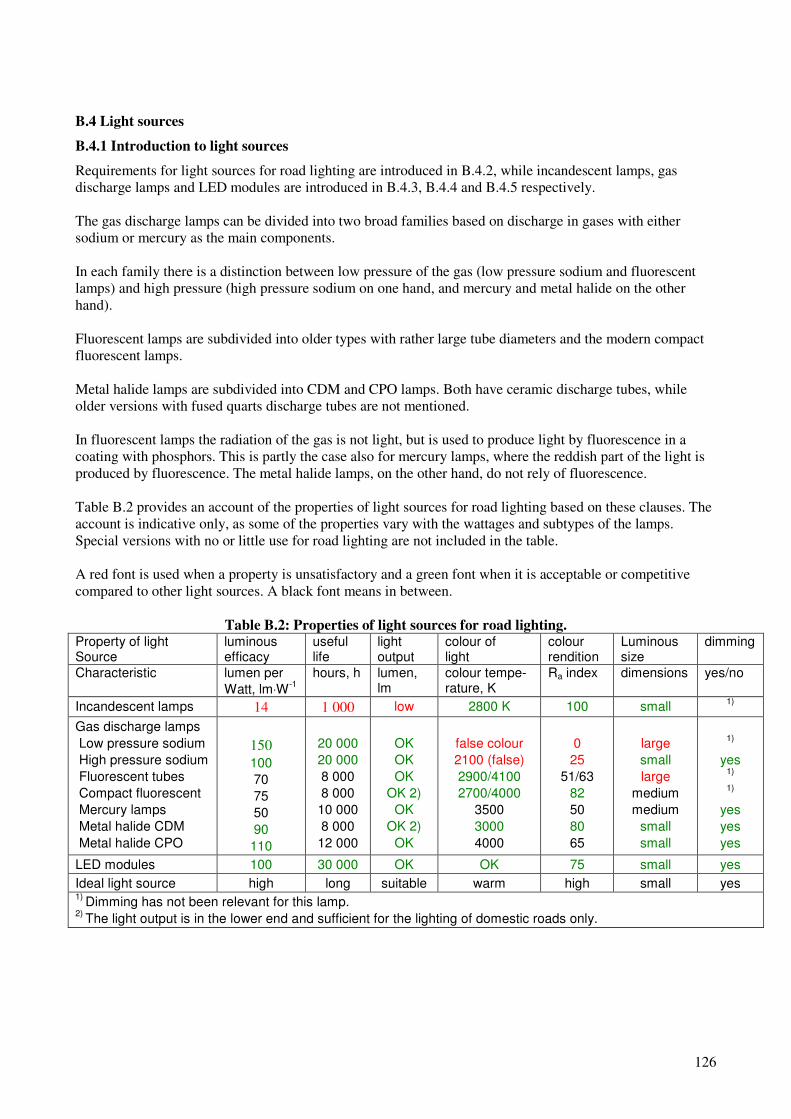
126

B.4 Light sources

B.4.1 Introduction to light sources

Requirements for light sources for road lighting are introduced in B.4.2, while incandescent lamps, gas

discharge lamps and LED modules are introduced in B.4.3, B.4.4 and B.4.5 respectively.

The gas discharge lamps can be divided into two broad families based on discharge in gases with either

sodium or mercury as the main components.

In each family there is a distinction between low pressure of the gas (low pressure sodium and fluorescent

lamps) and high pressure (high pressure sodium on one hand, and mercury and metal halide on the other

hand).


fluorescent lamps.





produced by fluorescence. The metal halide lamps, on the other hand, do not rely of fluorescence.

Table B.2 provides an account of the properties of light sources for road lighting based on these clauses. The

account is indicative only, as some of the properties vary with the wattages and subtypes of the lamps.

Special versions with no or little use for road lighting are not included in the table.

A red font is used when a property is unsatisfactory and a green font when it is acceptable or competitive

compared to other light sources. A black font means in between.

Table B.2: Properties of light sources for road lighting. Property of light Source

luminous efficacy

useful life

light output

colour of light

colour rendition

Luminous size

dimming


Watt, lm⋅W-1

hours, h lumen, lm

colour temperature, K


Incandescent lamps 14 1 000 low 2800 K 100 small 1)

Gas discharge lamps

Low pressure sodium

High pressure sodium

Fluorescent tubes

Compact fluorescent

Mercury lamps

Metal halide CDM

Metal halide CPO

150

100

70

75

50

90

110

20 000

20 000

8 000

8 000

10 000

8 000

12 000

OK

OK

OK

OK 2)

OK

OK 2)

OK

false colour

2100 (false)

2900/4100

2700/4000

3500

3000

4000

0

25

51/63

82

50

80

65

large

small

large

medium

medium

small

small

1)

yes 1)

1)

yes

yes

yes

LED modules 100 30 000 OK OK 75 small yes

Ideal light source high long suitable warm high small yes 1)

Dimming has not been relevant for this lamp. 2)

The light output is in the lower end and sufficient for the lighting of domestic roads only.

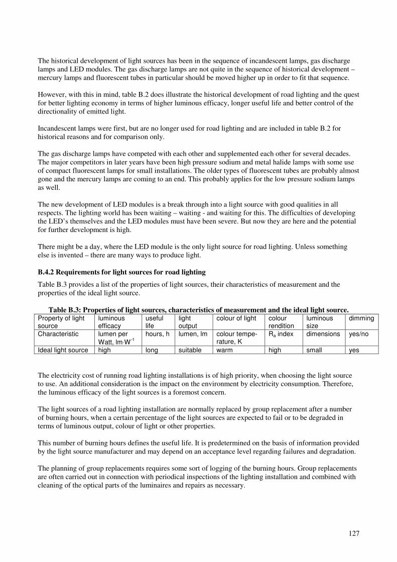
127

The historical development of light sources has been in the sequence of incandescent lamps, gas discharge

lamps and LED modules. The gas discharge lamps are not quite in the sequence of historical development –

mercury lamps and fluorescent tubes in particular should be moved higher up in order to fit that sequence.

However, with this in mind, table B.2 does illustrate the historical development of road lighting and the quest

for better lighting economy in terms of higher luminous efficacy, longer useful life and better control of the

directionality of emitted light.

Incandescent lamps were first, but are no longer used for road lighting and are included in table B.2 for

historical reasons and for comparison only.

The gas discharge lamps have competed with each other and supplemented each other for several decades.

The major competitors in later years have been high pressure sodium and metal halide lamps with some use

of compact fluorescent lamps for small installations. The older types of fluorescent tubes are probably almost

gone and the mercury lamps are coming to an end. This probably applies for the low pressure sodium lamps

as well.

The new development of LED modules is a break through into a light source with good qualities in all

respects. The lighting world has been waiting – waiting - and waiting for this. The difficulties of developing

the LED’s themselves and the LED modules must have been severe. But now they are here and the potential

for further development is high.

There might be a day, where the LED module is the only light source for road lighting. Unless something

else is invented – there are many ways to produce light.

B.4.2 Requirements for light sources for road lighting

Table B.3 provides a list of the properties of light sources, their characteristics of measurement and the

properties of the ideal light source.

Table B.3: Properties of light sources, characteristics of measurement and the ideal light source. Property of light source

luminous efficacy

useful life

light output

colour of light colour rendition

luminous size

dimming


Watt, lm⋅W-1

hours, h lumen, lm colour tempe-rature, K


Ideal light source high long suitable warm high small yes

The electricity cost of running road lighting installations is of high priority, when choosing the light source

to use. An additional consideration is the impact on the environment by electricity consumption. Therefore,

the luminous efficacy of the light sources is a foremost concern.

The light sources of a road lighting installation are normally replaced by group replacement after a number

of burning hours, when a certain percentage of the light sources are expected to fail or to be degraded in

terms of luminous output, colour of light or other properties.

This number of burning hours defines the useful life. It is predetermined on the basis of information provided

by the light source manufacturer and may depend on an acceptance level regarding failures and degradation.

The planning of group replacements requires some sort of logging of the burning hours. Group replacements

are often carried out in connection with periodical inspections of the lighting installation and combined with

cleaning of the optical parts of the luminaires and repairs as necessary.

128

NOTE: The alternative to group replacement is individual replacement of light sources that have failed or are visibly

depreciated. However, this is too expensive in labour cost in far the most cases.

Group replacements are relatively simple on some traffic areas, but complex on motorways and other high

speed traffic roads, where the work zone must be marked and often protected by heavy vehicles with crash

cushions. On some roads, the work can only be carried out at night with less traffic.

This involves costs that have increased with the cost of labour and traffic volume and also involves risks for

the workers and drivers. Therefore, the useful life of the light sources in another concern of high priority.

The light output has to be in the range that is useful for practical and conventional road lighting installations.

The total useful range of light output is perhaps 2 000 to 250 000 lm for road lighting in general, but for the

individual case it is quite small and depends on the road areas to be illuminated and the required lighting

level. This implies that a particular type of light source needs to be in different wattage versions with not too

large steps in order to cover a range of road lighting applications.

Light sources with warm colours of 2500 to 3000 K are usually preferred in the Nordic countries – at least

for the lighting of domestic roads. Planning of road lighting often involves some homogeneity of the colours

of light sources within a road network or an area for aesthetic reasons. For instance, light sources placed

close to each other or along a road should have similar colours of light.

It is generally agreed that colour rendition should be adequate on road areas that are lighted for pedestrians,

such as foot and cycle paths, domestic roads, pedestrians roads and even sidewalks and cycle paths along

traffic roads. In practice, priority has often been given to the efficiency of the road lighting, but this may

change with the availability of light sources with good colour rendition.

The luminous size of a light source has the significance that small dimensions allow optics that give better

control of the directionality of the light than large dimensions. Better control of the directionality has the

advantages of better aiming of the light towards the road areas to be illuminated and more freedom in the

lay-out of the lighting installations.

The development of optics for luminaires has actually gone hand in hand with the development of light

sources and has led to improvements of the lighting efficiency, the aesthetics of road lighting lay-out and

reductions of lighting nuisance such as undesirable lighting of properties and sky glow.

The possibility of dimming is an issue in those countries that use dimming at night for energy saving

purposes. All light sources can be dimmed in principle, but the equipment must be available and not too

complex and expensive. Additionally, the loss of luminous efficacy that is associated with dimming of most

light sources subtracts from the potential saving of energy and must not be too large.

Another matter not mentioned in table B.3 is the prize of the lamps, ballasts and control gear. It is a trend

that a new type of lamp is more expensive than and older type of lamp and that this can affect the

competition between the two.

B.4.3 Incandescent lamps

Incandescent lamps are based on thermal radiation as described in B.3.2.

Several improvements were made in a succession from Edison’s carbon filaments in vacuum bulbs to the use

of tantalium filaments and tungsten filaments in bulbs with inert gas filling. See figures B.17 and B.18.

129

Figure B.17: Edison’s first operational lamp of 1879.

Figure B.16: A modern standard incandescent lamp for general lighting.

The latest achievement was the halogen lamp, which was placed on the market in 1959. A small amount of

halogen is added to the filling of the bulb and reduces evaporation from the filament which can then be run at

a higher temperature.

Incandescent lamps are simple, cheap, operate directly on the voltage supply, have excellent properties in

terms of colour of light and colour rendition, are dimmable and well suited for use with reflectors. However,

the disadvantages of a low efficacy of typically 14 lm⋅W-1 and a short life, typically 1000 h are serious

indeed.

It seems not possible to raise the efficacy by a further raise of the temperature of the filament. Some attempts

have gone the other way – to reduce the power consumption by partly keeping the filament warm by means

of an IR reflecting coating on the inside of the bulb. This should raise the efficacy a good deal, but seems not

to have been commercially successful.

Therefore, the days of incandescent lamps in road lighting are gone, they ended in the 70’s. Thermal

radiation, however, still plays a small role. The discharge tubes of some of the high pressure discharge lamps

get so hot that thermal radiation provides a part of the light emission.

The days of incandescent lamps for indoor lighting are also coming to an end. Governments around the

world have passed measures to improve the energy efficiency of light bulbs used in homes and businesses.

Very often, these measures effectively ban the manufacture, importation or sale of current incandescent light

bulbs for general lighting. The aim is to increase the use and technological development of more energy-

efficient lighting alternatives, such as compact fluorescent lamps and LED lamps.

B.4.4 Gas discharge lamps

Gas discharge lamps are based on discharge in a gas as described in B.3.3.

130

Low pressure sodium lamps

Low-pressure sodium lamps (linear and U-shaped) were commercially introduced in 1932 and have been

subjected to continual improvements in materials and manufacturing technology over the years. They

produce light by discharge in sodium at low pressure. This produces a virtually monochromatic light

averaging a 589.3 nm wavelength (actually two dominant spectral lines very close together at 589.0 and

589.6 nm). It is a peculiar feature that these lamps need thermal insulation and have a larger vacuum

envelope with an infrared reflecting layer to that purpose. See figure B.19.

Figure B.19: A running low pressure sodium lamp.

The advantages of low pressure sodium lamps is a high luminous efficacy up to 200 lm⋅W-1 and a long life

up to 18 000 hours. Disadvantages are an ugly yellow colour of light, no colour rendition at all and large

dimensions of the luminous parts.

Low pressure sodium lamps have had extensive use for road lighting on motorways and other large traffic

roads in some countries and some or very little or no use in other countries. The use is declining in view of

the poor quality of the light and competition from other light sources that can be supplied with efficient

optics.


The first high pressure sodium lamps came on the market in 1960’s, but with a wattage and a luminous

output too high for most road lighting applications. The 150 and 250 Watt lamps appeared late 1970’s with

luminous outputs suitable for road lighting of most traffic roads and they soon gained use as replacements for

250 and 400 W mercury lamps. The later addition of 50, 70 and 100 Watt lamps made the high pressure

sodium lamp the most ubiquitous lamp for street lighting on the planet.

High-pressure sodium lamps produce light by discharge in sodium at a higher pressure and with additional

elements such as mercury. On account of spectral pressure broadening and the emissions from mercury, the

spectrum has some coverage of colours. Because of the extremely high chemical activity of the high pressure

sodium arc, the arc tube is ceramic, made of translucent aluminium oxide.

The advantages of high pressure sodium lamps are the same as for the low pressure sodium lamp, a high

efficacy and a long life. The luminous efficacy is about 100 lm⋅W-1 - and even higher for the high wattage

lamps.

The useful life is approximately 20 000 hours. It ends in a peculiar “cycling”, where a lamp turns itself off,

cools down, restarts, warms up etc.

An additional advantage is the small size of the luminous parts. The high pressure sodium lamps of suitable

wattages appeared first with frosted bulbs of the same elliptical shape and sizes as the mercury lamps they

were replacing. This allowed reuse of the optics developed for mercury lamps. Later versions with clear

bulbs allowed development of more efficient optics. Refer to figure B.20.

High pressure sodium lamps can be dimmed individually by switching from the normal ballast to a ballast

with a higher reactive resistance. Another method with widespread use in Denmark is to reduce the voltage

to a group of lamps and luminaires by means of an autotransformer. The energy saving is approximately 35

% at a dimming level of 50 %.

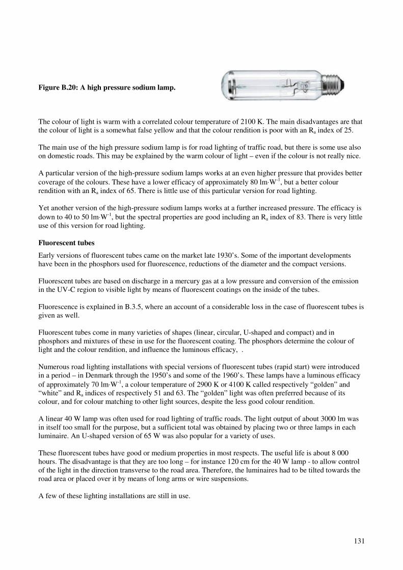
131

Figure B.20: A high pressure sodium lamp.

The colour of light is warm with a correlated colour temperature of 2100 K. The main disadvantages are that

the colour of light is a somewhat false yellow and that the colour rendition is poor with an Ra index of 25.

The main use of the high pressure sodium lamp is for road lighting of traffic road, but there is some use also

on domestic roads. This may be explained by the warm colour of light – even if the colour is not really nice.

A particular version of the high-pressure sodium lamps works at an even higher pressure that provides better

coverage of the colours. These have a lower efficacy of approximately 80 lm⋅W-1, but a better colour

rendition with an Ra index of 65. There is little use of this particular version for road lighting.

Yet another version of the high-pressure sodium lamps works at a further increased pressure. The efficacy is

down to 40 to 50 lm⋅W-1, but the spectral properties are good including an Ra index of 83. There is very little

use of this version for road lighting.

Fluorescent tubes

Early versions of fluorescent tubes came on the market late 1930’s. Some of the important developments

have been in the phosphors used for fluorescence, reductions of the diameter and the compact versions.

Fluorescent tubes are based on discharge in a mercury gas at a low pressure and conversion of the emission

in the UV-C region to visible light by means of fluorescent coatings on the inside of the tubes.

Fluorescence is explained in B.3.5, where an account of a considerable loss in the case of fluorescent tubes is

given as well.

Fluorescent tubes come in many varieties of shapes (linear, circular, U-shaped and compact) and in

phosphors and mixtures of these in use for the fluorescent coating. The phosphors determine the colour of

light and the colour rendition, and influence the luminous efficacy, .

Numerous road lighting installations with special versions of fluorescent tubes (rapid start) were introduced

in a period – in Denmark through the 1950’s and some of the 1960’s. These lamps have a luminous efficacy

of approximately 70 lm⋅W-1, a colour temperature of 2900 K or 4100 K called respectively “golden” and

“white” and Ra indices of respectively 51 and 63. The “golden” light was often preferred because of its

colour, and for colour matching to other light sources, despite the less good colour rendition.

A linear 40 W lamp was often used for road lighting of traffic roads. The light output of about 3000 lm was

in itself too small for the purpose, but a sufficient total was obtained by placing two or three lamps in each

luminaire. An U-shaped version of 65 W was also popular for a variety of uses.

These fluorescent tubes have good or medium properties in most respects. The useful life is about 8 000

hours. The disadvantage is that they are too long – for instance 120 cm for the 40 W lamp - to allow control

of the light in the direction transverse to the road area. Therefore, the luminaires had to be tilted towards the

road area or placed over it by means of long arms or wire suspensions.

A few of these lighting installations are still in use.

132

More modern compact fluorescent light bulbs have since gained some use for small road lighting

installations on for instance domestic roads. The efficacy and the useful life has not been improved compared

to the above (70 lm⋅W-1 and 8 000 hours), but the dimensions have been reduced drastically. The colour of

light is a choice from warm to cool and the colour rendition is good with an Ra index above 80. The

luminous output is up to 3200 lm for a 36 W lamp.

Mercury lamps

Mercury lamps have a long history resulting in the modern mercury lamp in 1936.

Mercury lamps are based on discharge in a mercury gas at a high pressure in a small discharge tube in fused

quartz. Compared to fluorescent tubes, this provides emission at some additional lines, including strong lines

in the violet and green. An exterior glass bulb has an inner fluorescent coating that adds mainly red light to

the spectrum. The construction and appearance is illustrated in figure B.21.

Figure B.21: The construction and appearance of a high pressure mercury lamp.

The luminous efficacy is 40 to 60 lm⋅W-1 with the highest values for the high wattage lamps. The light is a

bit cool with a colour temperature of 3500 K. The colour rendition is rather poor with an Ra index of

approximately 50.

The life is often indicated as long – like 20 000 hours. However, the luminous output and the quality of the

light degrade strongly during such a period due to degradation of the fluorescent coating. These lamps in fact

rarely burn out, but end with a weak green light if not replaced. The useful life should, therefore, be put

substantially lower, for instance at 10 000 hours.

A particular version of the mercury lamp, the QL lamp is not run by gas discharge, but by excitation of the

gas by an electromagnetic field. Compared to the mercury lamp it has a much longer life, a much better

colour rendition and a higher efficacy. It should have outcompeted the mercury lamp – but has been too

expensive.

The advantage of the mercury lamps compared to fluorescent tubes lies in the smaller dimensions of the

luminous parts. These are given by the approximately ellipsoidal shape of the exterior bulb. The size of the

ellipsoid depends on the lamp wattage. As an example, the width is 7,6 cm and the length is 12 cm for the

125 W lamp.

These dimensions are sufficiently small to allow for optics that direct the light both longitudinally and

transverse to the road so that use of large tilts and long arms can be avoided. This made the mercury lamps

popular for road lighting of traffic roads in a period ending with the advent of the far more efficient high

pressure sodium lamp.

133

The mercury lamps kept its popularity for other road lighting purposes, such as the lighting of domestic

roads and city areas.

There is a process on eliminating the use of mercury lamps for road lighting and other lighting on the basis

of the Ecodesign or EuP Directive 2005/32/EC by the EU Commission. The long history of mercury lamps is

coming to an end.

Metal halide lamps

Metal halide lamps are relatively new compared to other discharge lamps. They produce light by an electric

arc through a gaseous mixture of vaporized mercury and metal halides (compounds of metals with bromine

or iodine). They are similar to high pressure mercury lamps, but rely on the metal halides to produce visible

light in stead of fluorescence in a phosphor coating. The exterior glass bulb has a coating to filter out the

ultraviolet light produced.

Metal halide lamps were not used, or at least not used much, for road lighting until the ceramic discharge

metal-halide (CDM) lamp emerged in the 1990’s. These lamps contain the discharge in ceramic tubes,

usually made of sintered alumina, similar to the ceramic tubes of the high pressure sodium lamps. The

advantage of the ceramic tubes, compared to fused quarts tubes, lies in their resistance to penetration by

metal ions.

The luminous efficacy of a CDM lamp is about 90 lm⋅W-1. The light is warm with a colour temperature of

3000 K. The colour rendition is good with an Ra index of approximately 80. The useful life is about 8 000

hours. The small ceramic tube is the luminous part.

Another more recent version of the ceramic discharge metal-halide lamp, the CPO lamp, has a higher

efficacy of 115 lm⋅W-1 and a longer useful life of about 12 000 hours. The cost of this is a higher colour

temperature of 4000 K and a somewhat lower Ra index of 60 to 70. This lamp is a real competitor to the high

pressure sodium lamp. A CPO lamp is shown in figure B.22.

CDM and CPO lamps can be dimmed by means of electronic ballasts.

Figure B.22: A metal halide lamp (CPO).

Ballasts for gas discharge lamps

Gas discharge lamps do not - unlike incandescent lamps - in themselves control the current. If they were

connected to a constant-voltage power supply, they would draw an increasing amount of current until

becoming destroyed or cause the power supply to fail. Therefore, they require auxiliary equipment to control

current flow through the gas. This equipment may be a conventional reactive ballast or it may be an

electronic ballast

A reactive ballast consists of a coil of copper wire around an iron core that provides a reactive resistance. A

reactive ballast is also called a magnetic ballast or an inductor. It is placed in series with the gas discharge

lamp.

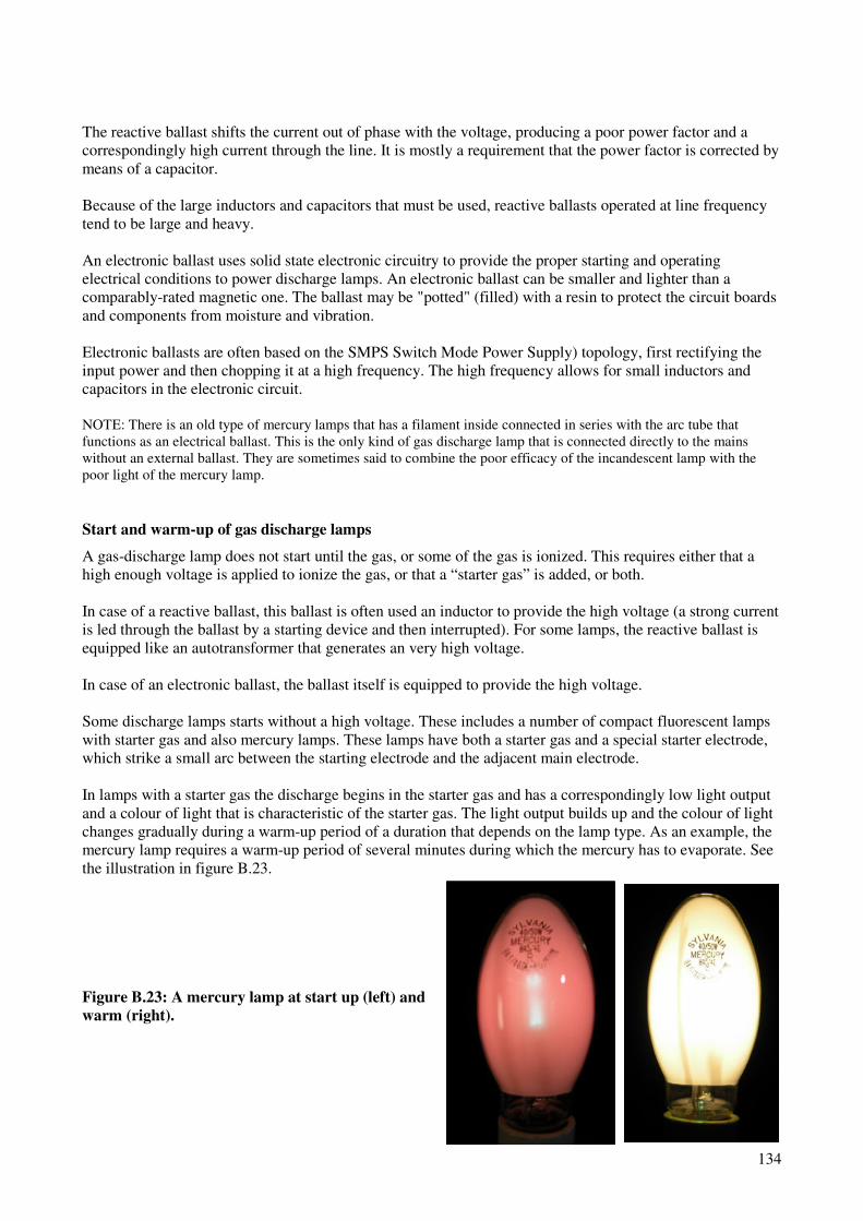
134

The reactive ballast shifts the current out of phase with the voltage, producing a poor power factor and a

correspondingly high current through the line. It is mostly a requirement that the power factor is corrected by

means of a capacitor.

Because of the large inductors and capacitors that must be used, reactive ballasts operated at line frequency

tend to be large and heavy.

An electronic ballast uses solid state electronic circuitry to provide the proper starting and operating

electrical conditions to power discharge lamps. An electronic ballast can be smaller and lighter than a

comparably-rated magnetic one. The ballast may be "potted" (filled) with a resin to protect the circuit boards

and components from moisture and vibration.

Electronic ballasts are often based on the SMPS Switch Mode Power Supply) topology, first rectifying the

input power and then chopping it at a high frequency. The high frequency allows for small inductors and

capacitors in the electronic circuit.

NOTE: There is an old type of mercury lamps that has a filament inside connected in series with the arc tube that

functions as an electrical ballast. This is the only kind of gas discharge lamp that is connected directly to the mains

without an external ballast. They are sometimes said to combine the poor efficacy of the incandescent lamp with the

poor light of the mercury lamp.

Start and warm-up of gas discharge lamps

A gas-discharge lamp does not start until the gas, or some of the gas is ionized. This requires either that a

high enough voltage is applied to ionize the gas, or that a “starter gas” is added, or both.

In case of a reactive ballast, this ballast is often used an inductor to provide the high voltage (a strong current

is led through the ballast by a starting device and then interrupted). For some lamps, the reactive ballast is

equipped like an autotransformer that generates an very high voltage.

In case of an electronic ballast, the ballast itself is equipped to provide the high voltage.

Some discharge lamps starts without a high voltage. These includes a number of compact fluorescent lamps

with starter gas and also mercury lamps. These lamps have both a starter gas and a special starter electrode,

which strike a small arc between the starting electrode and the adjacent main electrode.

In lamps with a starter gas the discharge begins in the starter gas and has a correspondingly low light output

and a colour of light that is characteristic of the starter gas. The light output builds up and the colour of light

changes gradually during a warm-up period of a duration that depends on the lamp type. As an example, the

mercury lamp requires a warm-up period of several minutes during which the mercury has to evaporate. See

the illustration in figure B.23.

Figure B.23: A mercury lamp at start up (left) and

warm (right).

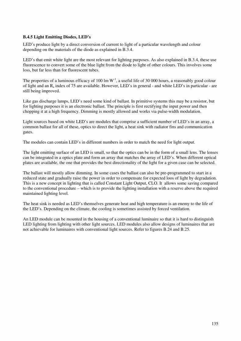
135

B.4.5 Light Emitting Diodes, LED’s

LED’s produce light by a direct conversion of current to light of a particular wavelength and colour

depending on the materials of the diode as explained in B.3.4.

LED’s that emit white light are the most relevant for lighting purposes. As also explained in B.3.4, these use

fluorescence to convert some of the blue light from the diode to light of other colours. This involves some

loss, but far less than for fluorescent tubes.

The properties of a luminous efficacy of 100 lm⋅W-1, a useful life of 30 000 hours, a reasonably good colour

of light and an Ra index of 75 are available. However, LED’s in general - and white LED’s in particular - are

still being improved.

Like gas discharge lamps, LED’s need some kind of ballast. In primitive systems this may be a resistor, but

for lighting purposes it is an electronic ballast. The principle is first rectifying the input power and then

chopping it at a high frequency. Dimming is mostly allowed and works via pulse-width modulation.

Light sources based on white LED’s are modules that comprise a sufficient number of LED’s in an array, a

common ballast for all of these, optics to direct the light, a heat sink with radiator fins and communication

gates.

The modules can contain LED’s in different numbers in order to match the need for light output.

The light emitting surface of an LED is small, so that the optics can be in the form of a small lens. The lenses

can be integrated in a optics plate and form an array that matches the array of LED’s. When different optical

plates are available, the one that provides the best directionality of the light for a given case can be selected.

The ballast will mostly allow dimming. In some cases the ballast can also be pre-programmed to start in a

reduced state and gradually raise the power in order to compensate for expected loos of light by degradation.

This is a new concept in lighting that is called Constant Light Output, CLO. It allows some saving compared

to the conventional procedure – which is to provide the lighting installation with a reserve above the required

maintained lighting level.

The heat sink is needed as LED’s themselves generate heat and high temperature is an enemy to the life of

the LED’s. Depending on the climate, the cooling is sometimes assisted by forced ventilation.

An LED module can be mounted in the housing of a conventional luminaire so that it is hard to distinguish

LED lighting from lighting with other light sources. LED modules also allow designs of luminaires that are

not achievable for luminaires with conventional light sources. Refer to figures B.24 and B.25.

136

Figure B.24: Conventional luminaires with

LED modules.

Figure B.25: An example of a flat design of

an LED luminaire.

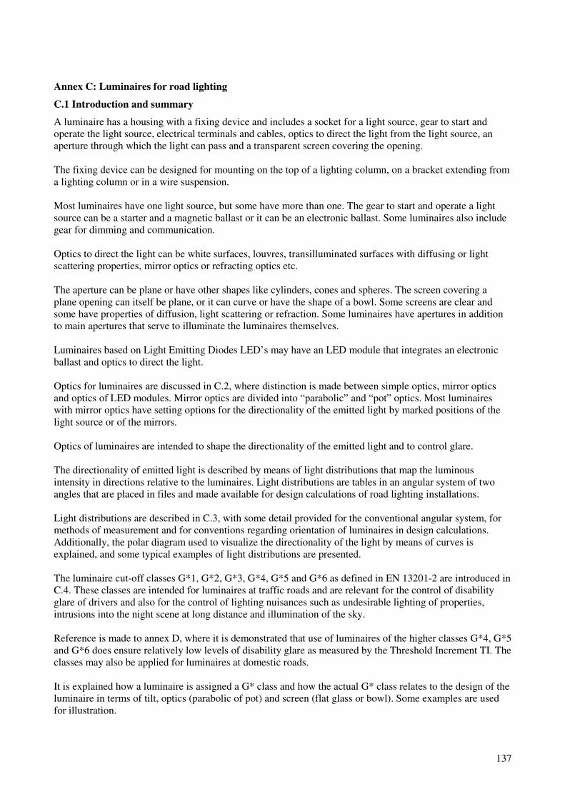
137

Annex C: Luminaires for road lighting

C.1 Introduction and summary

A luminaire has a housing with a fixing device and includes a socket for a light source, gear to start and

operate the light source, electrical terminals and cables, optics to direct the light from the light source, an

aperture through which the light can pass and a transparent screen covering the opening.

The fixing device can be designed for mounting on the top of a lighting column, on a bracket extending from

a lighting column or in a wire suspension.

Most luminaires have one light source, but some have more than one. The gear to start and operate a light

source can be a starter and a magnetic ballast or it can be an electronic ballast. Some luminaires also include

gear for dimming and communication.

Optics to direct the light can be white surfaces, louvres, transilluminated surfaces with diffusing or light

scattering properties, mirror optics or refracting optics etc.

The aperture can be plane or have other shapes like cylinders, cones and spheres. The screen covering a

plane opening can itself be plane, or it can curve or have the shape of a bowl. Some screens are clear and

some have properties of diffusion, light scattering or refraction. Some luminaires have apertures in addition

to main apertures that serve to illuminate the luminaires themselves.

Luminaires based on Light Emitting Diodes LED’s may have an LED module that integrates an electronic

ballast and optics to direct the light.

Optics for luminaires are discussed in C.2, where distinction is made between simple optics, mirror optics

and optics of LED modules. Mirror optics are divided into “parabolic” and “pot” optics. Most luminaires

with mirror optics have setting options for the directionality of the emitted light by marked positions of the

light source or of the mirrors.

Optics of luminaires are intended to shape the directionality of the emitted light and to control glare.

The directionality of emitted light is described by means of light distributions that map the luminous

intensity in directions relative to the luminaires. Light distributions are tables in an angular system of two

angles that are placed in files and made available for design calculations of road lighting installations.

Light distributions are described in C.3, with some detail provided for the conventional angular system, for

methods of measurement and for conventions regarding orientation of luminaires in design calculations.

Additionally, the polar diagram used to visualize the directionality of the light by means of curves is

explained, and some typical examples of light distributions are presented.

The luminaire cut-off classes G*1, G*2, G*3, G*4, G*5 and G*6 as defined in EN 13201-2 are introduced in

C.4. These classes are intended for luminaires at traffic roads and are relevant for the control of disability

glare of drivers and also for the control of lighting nuisances such as undesirable lighting of properties,

intrusions into the night scene at long distance and illumination of the sky.

Reference is made to annex D, where it is demonstrated that use of luminaires of the higher classes G*4, G*5

and G*6 does ensure relatively low levels of disability glare as measured by the Threshold Increment TI. The

classes may also be applied for luminaires at domestic roads.

It is explained how a luminaire is assigned a G* class and how the actual G* class relates to the design of the

luminaire in terms of tilt, optics (parabolic of pot) and screen (flat glass or bowl). Some examples are used

for illustration.

138

The luminaire glare index classes D1, D2, D3, D4, D5 and D6 as defined in EN 13201-2 are introduced in

C.5. These classes are intended for luminaires at road areas lit for the benefit of pedestrians and pedal cyclists

and are relevant for the control of discomfort glare for these road users. Such luminaires are mostly of the

lantern type with emphasis on design and aesthetical appearance.

It is explained how a luminaire is assigned a D class and why useful restrictions of discomfort glare are

provided mainly by the classes D5 and D6. Further, the link to the “Unified Glare Rating method” for indoor

work places is accounted for. The conclusion is that these classes serve to avoid that luminaires – in particular

of the lantern type – become strongly offensive by the use of lamps of a high output compared to the size of the

luminous parts.

Luminaires are generally subject to requirements on an international or national level. In Europe, the

directives on low voltage and EMC apply. The low voltage directive provides requirements for not only

electrical safety, but also safety against components falling down and marking. Markings shall be clear and

durable and include:

- Manufacturer, type designation and type of light source

- Encapsulation class (IP class)

- Electric isolation class

- setting options

- circuit diagram

- electrical terminals.

An example of requirements on a national level is given by the Danish tender specifications “AAB for

belysningsmateriel”. They include among else:

- connection to the phases

- encapsulation class

- avoidance of accumulation of water by condensation

- tightness to insects

- protection against vandalism

- access for cleaning and lamp replacement

- safety against falling parts

- durability against vibration

- resistance against soiling, cleaning, corrosion, weather and climate

- types of acceptable materials

- solidity

- variations of supply voltage

- electrical insulation class II

- inclusion of all electric components within the luminaire

- ballasts and starters in accordance with IEC provisions

- starting capability in temperatures from -20 °C to +40 °C

- capability to use light sources from at least two manufacturers

- load relief of electric cables

- user instructions including assembly, settings and cleaning

- documentation that the luminaire can provide compliance with the lighting requirements for specified

lighting installations.

139

C.2 Optics for luminaires

C.2.1 Simple optics

Most luminaires have optics to prevent a direct view to the light source and/or to direct the light towards

areas to be illuminated.

Some luminaires that are intended for the lighting of domestic roads, pedestrians road, paths, cycle ways,

parking lots etc. have simple optics combined with a decorative design. These are called lanterns in the

following. A few examples are shown in figure C.1

Figure C.1: Examples of lanterns.

Lanterns often use elements like glare screens or louvres, top surfaces with diffuse reflection, panels with

diffuse transmission or scattering. The light distribution is often with rotational symmetry. Lanterns are

mounted on columns on the road area or close to it.

Older types of luminaires for long light sources like linear fluorescent tubes also have simple optics. The

light distributions are symmetrical with respect to two vertical planes – one through the tube axis and one

perpendicular to that. Light distributions with these symmetries are said to be symmetrical.

Such older luminaires were mostly mounted with the long axis transverse to the road and had in some cases

optics in the form of mirrors of refractors to throw light in the longitudinal direction of the road. When

mounted at the side of the road, they were tilted upwards and/or mounted on brackets towards the area. A

couple of examples are shown in figure C.2.

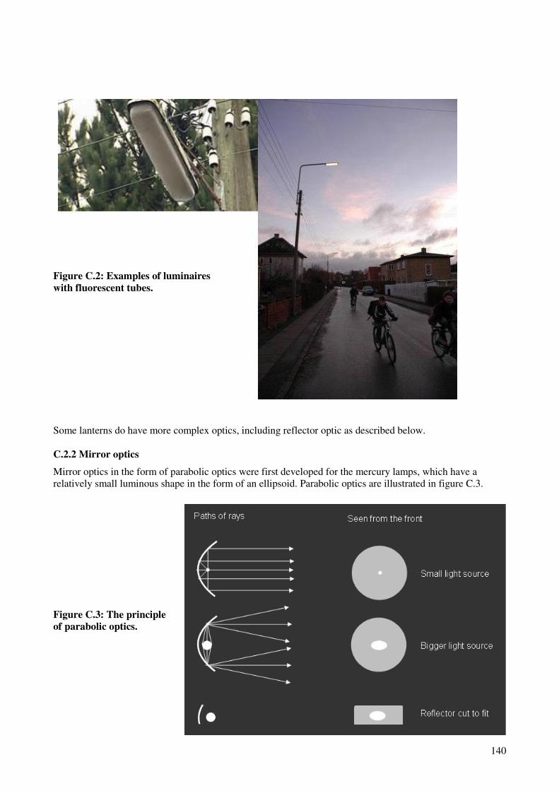
140

Figure C.2: Examples of luminaires

with fluorescent tubes.

Some lanterns do have more complex optics, including reflector optic as described below.

C.2.2 Mirror optics

Mirror optics in the form of parabolic optics were first developed for the mercury lamps, which have a

relatively small luminous shape in the form of an ellipsoid. Parabolic optics are illustrated in figure C.3.

Figure C.3: The principle

of parabolic optics.

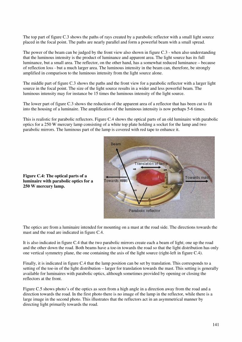
141

The top part of figure C.3 shows the paths of rays created by a parabolic reflector with a small light source

placed in the focal point. The paths are nearly parallel and form a powerful beam with a small spread.

The power of the beam can be judged by the front view also shown in figure C.3 - when also understanding

that the luminous intensity is the product of luminance and apparent area. The light source has its full

luminance, but a small area. The reflector, on the other hand, has a somewhat reduced luminance – because

of reflection loss - but a much larger area. The luminous intensity in the beam can, therefore, be strongly

amplified in comparison to the luminous intensity from the light source alone.

The middle part of figure C.3 shows the paths and the front view for a parabolic reflector with a larger light

source in the focal point. The size of the light source results in a wider and less powerful beam. The

luminous intensity may for instance be 15 times the luminous intensity of the light source.

The lower part of figure C.3 shows the reduction of the apparent area of a reflector that has been cut to fit

into the housing of a luminaire. The amplification of the luminous intensity is now perhaps 5-6 times.

This is realistic for parabolic reflectors. Figure C.4 shows the optical parts of an old luminaire with parabolic

optics for a 250 W mercury lamp consisting of a white top plate holding a socket for the lamp and two

parabolic mirrors. The luminous part of the lamp is covered with red tape to enhance it.

Figure C.4: The optical parts of a

luminaire with parabolic optics for a

250 W mercury lamp.

The optics are from a luminaire intended for mounting on a mast at the road side. The directions towards the

mast and the road are indicated in figure C.4.

It is also indicated in figure C.4 that the two parabolic mirrors create each a beam of light; one up the road

and the other down the road. Both beams have a toe-in towards the road so that the light distribution has only

one vertical symmetry plane, the one containing the axis of the light source (right-left in figure C.4).

Finally, it is indicated in figure C.4 that the lamp position can be set by translation. This corresponds to a

setting of the toe-in of the light distribution – larger for translation towards the mast. This setting is generally

available for luminaires with parabolic optics, although sometimes provided by opening or closing the

reflectors at the front.

Figure C.5 shows photo’s of the optics as seen from a high angle in a direction away from the road and a

direction towards the road. In the first photo there is no image of the lamp in the reflector, while there is a

large image in the second photo. This illustrates that the reflectors act in an asymmetrical manner by

directing light primarily towards the road.

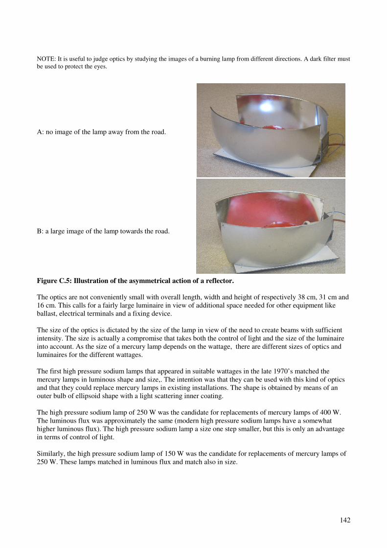
142

NOTE: It is useful to judge optics by studying the images of a burning lamp from different directions. A dark filter must

be used to protect the eyes.

A: no image of the lamp away from the road.

B: a large image of the lamp towards the road.

Figure C.5: Illustration of the asymmetrical action of a reflector.

The optics are not conveniently small with overall length, width and height of respectively 38 cm, 31 cm and

16 cm. This calls for a fairly large luminaire in view of additional space needed for other equipment like

ballast, electrical terminals and a fixing device.

The size of the optics is dictated by the size of the lamp in view of the need to create beams with sufficient

intensity. The size is actually a compromise that takes both the control of light and the size of the luminaire

into account. As the size of a mercury lamp depends on the wattage, there are different sizes of optics and

luminaires for the different wattages.

The first high pressure sodium lamps that appeared in suitable wattages in the late 1970’s matched the

mercury lamps in luminous shape and size,. The intention was that they can be used with this kind of optics

and that they could replace mercury lamps in existing installations. The shape is obtained by means of an

outer bulb of ellipsoid shape with a light scattering inner coating.

The high pressure sodium lamp of 250 W was the candidate for replacements of mercury lamps of 400 W.

The luminous flux was approximately the same (modern high pressure sodium lamps have a somewhat

higher luminous flux). The high pressure sodium lamp a size one step smaller, but this is only an advantage

in terms of control of light.

Similarly, the high pressure sodium lamp of 150 W was the candidate for replacements of mercury lamps of

250 W. These lamps matched in luminous flux and match also in size.

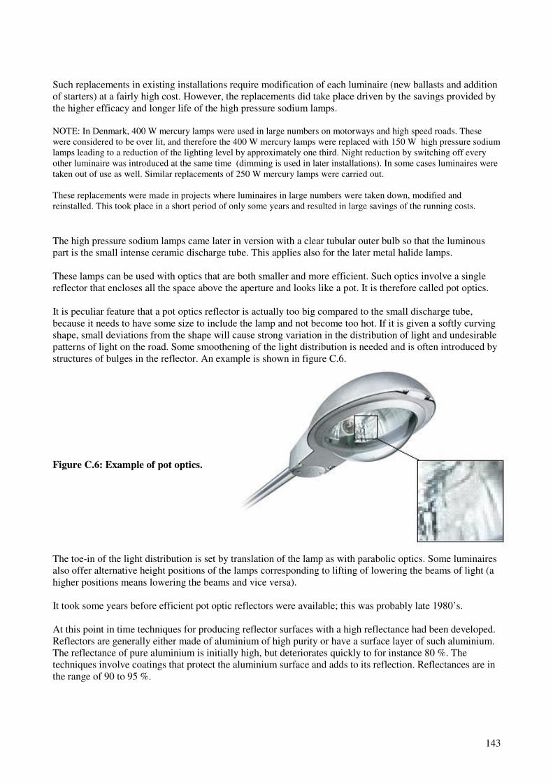
143

Such replacements in existing installations require modification of each luminaire (new ballasts and addition

of starters) at a fairly high cost. However, the replacements did take place driven by the savings provided by

the higher efficacy and longer life of the high pressure sodium lamps.

NOTE: In Denmark, 400 W mercury lamps were used in large numbers on motorways and high speed roads. These

were considered to be over lit, and therefore the 400 W mercury lamps were replaced with 150 W high pressure sodium

lamps leading to a reduction of the lighting level by approximately one third. Night reduction by switching off every

other luminaire was introduced at the same time (dimming is used in later installations). In some cases luminaires were

taken out of use as well. Similar replacements of 250 W mercury lamps were carried out.

These replacements were made in projects where luminaires in large numbers were taken down, modified and

reinstalled. This took place in a short period of only some years and resulted in large savings of the running costs.

The high pressure sodium lamps came later in version with a clear tubular outer bulb so that the luminous

part is the small intense ceramic discharge tube. This applies also for the later metal halide lamps.

These lamps can be used with optics that are both smaller and more efficient. Such optics involve a single

reflector that encloses all the space above the aperture and looks like a pot. It is therefore called pot optics.

It is peculiar feature that a pot optics reflector is actually too big compared to the small discharge tube,

because it needs to have some size to include the lamp and not become too hot. If it is given a softly curving

shape, small deviations from the shape will cause strong variation in the distribution of light and undesirable

patterns of light on the road. Some smoothening of the light distribution is needed and is often introduced by

structures of bulges in the reflector. An example is shown in figure C.6.

Figure C.6: Example of pot optics.

The toe-in of the light distribution is set by translation of the lamp as with parabolic optics. Some luminaires

also offer alternative height positions of the lamps corresponding to lifting of lowering the beams of light (a

higher positions means lowering the beams and vice versa).

It took some years before efficient pot optic reflectors were available; this was probably late 1980’s.

At this point in time techniques for producing reflector surfaces with a high reflectance had been developed.

Reflectors are generally either made of aluminium of high purity or have a surface layer of such aluminium.

The reflectance of pure aluminium is initially high, but deteriorates quickly to for instance 80 %. The

techniques involve coatings that protect the aluminium surface and adds to its reflection. Reflectances are in

the range of 90 to 95 %.

144

As pot optics reflectors have surfaces of high reflection as an additional advantage to the older forms of

parabolic optics, they raised the efficiency of luminaires from typically 70 % to 80 %. The improvement in

lighting efficiency is higher because of the improved control of the directionality of the light.

Luminaires to be mounted in wire suspension above the road have special versions of reflector optics that

produce symmetrical light distributions. An example of such a luminaire is shown in figure C.7.

Figure C.7: A luminaire in wire suspension.

Luminaires with reflector optics are used not only on traffic roads, but also on domestic roads and other road

areas for pedestrians and cyclists, where they compete with lanterns.

C.2.3 Optics for LED modules

It may some day be possible to make a compact light source based on LED’s that can be used with optics as

described above. With the present technology, it is necessary to use several LED’s placed in arrays that are a

bit large for use with reflectors.

Therefore, the light from each LED is often directed individually, with each LED forming a beam of some

width shaped by refracting and/or reflecting optics. The complete light distribution is added up by the beams

from the individual LED’s. There are probably several variations of this theme on the market, and new

variations being developed.

The first LED luminaires used pointing of the LED’s and their optics as an instrument. This raises the

problem in connection with road lighting of traffic roads that there is a need to set the light distributions to

match the need for the individual installations.

At least one of the solutions is elegant. It is to mount the LED’s in a matrix and provide a plate with

individual refractive optics for each of the LED’s. The optics plate determines the light distribution and

change of the optics plate changes the light distribution. It is probably expensive to develop a sufficient

number of optics plates, but cheap to produce them by moulding.

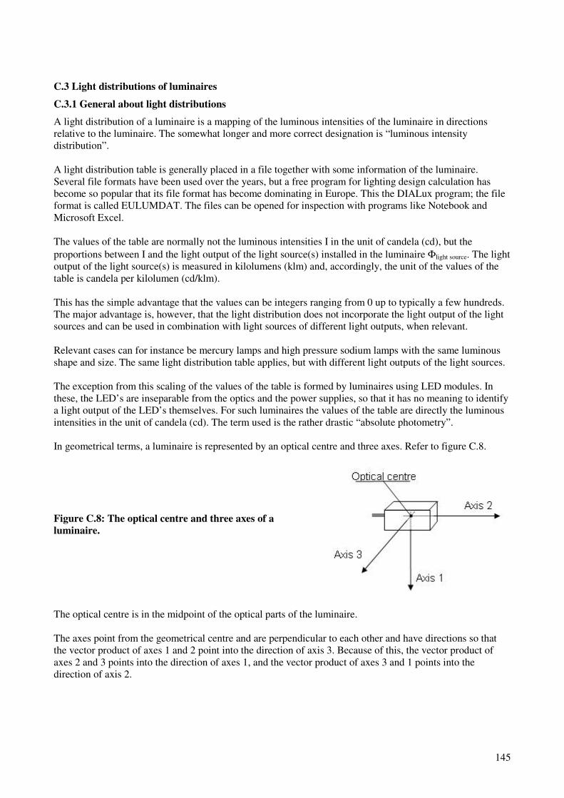
145

C.3 Light distributions of luminaires

C.3.1 General about light distributions

A light distribution of a luminaire is a mapping of the luminous intensities of the luminaire in directions

relative to the luminaire. The somewhat longer and more correct designation is “luminous intensity

distribution”.

A light distribution table is generally placed in a file together with some information of the luminaire.

Several file formats have been used over the years, but a free program for lighting design calculation has

become so popular that its file format has become dominating in Europe. This the DIALux program; the file

format is called EULUMDAT. The files can be opened for inspection with programs like Notebook and

Microsoft Excel.

The values of the table are normally not the luminous intensities I in the unit of candela (cd), but the

proportions between I and the light output of the light source(s) installed in the luminaire Φlight source. The light

output of the light source(s) is measured in kilolumens (klm) and, accordingly, the unit of the values of the

table is candela per kilolumen (cd/klm).

This has the simple advantage that the values can be integers ranging from 0 up to typically a few hundreds.

The major advantage is, however, that the light distribution does not incorporate the light output of the light

sources and can be used in combination with light sources of different light outputs, when relevant.

Relevant cases can for instance be mercury lamps and high pressure sodium lamps with the same luminous

shape and size. The same light distribution table applies, but with different light outputs of the light sources.

The exception from this scaling of the values of the table is formed by luminaires using LED modules. In

these, the LED’s are inseparable from the optics and the power supplies, so that it has no meaning to identify

a light output of the LED’s themselves. For such luminaires the values of the table are directly the luminous

intensities in the unit of candela (cd). The term used is the rather drastic “absolute photometry”.

In geometrical terms, a luminaire is represented by an optical centre and three axes. Refer to figure C.8.

Figure C.8: The optical centre and three axes of a

luminaire.

The optical centre is in the midpoint of the optical parts of the luminaire.

The axes point from the geometrical centre and are perpendicular to each other and have directions so that

the vector product of axes 1 and 2 point into the direction of axis 3. Because of this, the vector product of

axes 2 and 3 points into the direction of axes 1, and the vector product of axes 3 and 1 points into the

direction of axis 2.

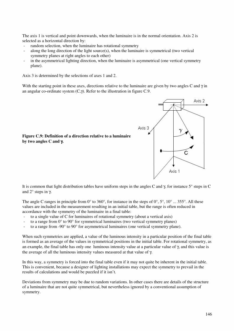
146

The axis 1 is vertical and point downwards, when the luminaire is in the normal orientation. Axis 2 is

selected as a horizontal direction by:

- random selection, when the luminaire has rotational symmetry

- along the long direction of the light source(s), when the luminaire is symmetrical (two vertical

symmetry planes at right angles to each other)

- in the asymmetrical lighting direction, when the luminaire is asymmetrical (one vertical symmetry

plane).

Axis 3 is determined by the selections of axes 1 and 2.

With the starting point in these axes, directions relative to the luminaire are given by two angles C and γ in

an angular co-ordinate system (C,γ). Refer to the illustration in figure C.9.

Figure C.9: Definition of a direction relative to a luminaire

by two angles C and γγγγ.

It is common that light distribution tables have uniform steps in the angles C and γ, for instance 5° steps in C

and 2° steps in γ.

The angle C ranges in principle from 0° to 360°, for instance in the steps of 0°, 5°, 10° ... 355°. All these

values are included in the measurement resulting in an initial table, but the range is often reduced in

accordance with the symmetry of the luminaire in a final table:

- to a single value of C for luminaires of rotational symmetry (about a vertical axis)

- to a range from 0° to 90° for symmetrical luminaires (two vertical symmetry planes)

- to a range from -90° to 90° for asymmetrical luminaires (one vertical symmetry plane).

When such symmetries are applied, a value of the luminous intensity in a particular position of the final table

is formed as an average of the values in symmetrical positions in the initial table. For rotational symmetry, as

an example, the final table has only one luminous intensity value at a particular value of γ, and this value is

the average of all the luminous intensity values measured at that value of γ.

In this way, a symmetry is forced into the final table even if it may not quite be inherent in the initial table.

This is convenient, because a designer of lighting installations may expect the symmetry to prevail in the

results of calculations and would be puzzled if it isn’t.

Deviations from symmetry may be due to random variations. In other cases there are details of the structure

of a luminaire that are not quite symmetrical, but nevertheless ignored by a conventional assumption of

symmetry.

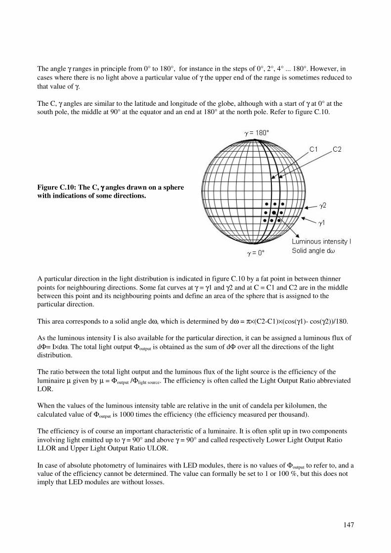
147

The angle γ ranges in principle from 0° to 180°, for instance in the steps of 0°, 2°, 4° ... 180°. However, in

cases where there is no light above a particular value of γ the upper end of the range is sometimes reduced to

that value of γ.

The C, γ angles are similar to the latitude and longitude of the globe, although with a start of γ at 0° at the

south pole, the middle at 90° at the equator and an end at 180° at the north pole. Refer to figure C.10.

Figure C.10: The C, γγγγ angles drawn on a sphere

with indications of some directions.

A particular direction in the light distribution is indicated in figure C.10 by a fat point in between thinner

points for neighbouring directions. Some fat curves at γ = γ1 and γ2 and at C = C1 and C2 are in the middle

between this point and its neighbouring points and define an area of the sphere that is assigned to the

particular direction.

This area corresponds to a solid angle dω, which is determined by dω = π×(C2-C1)×(cos(γ1)- cos(γ2))/180.

As the luminous intensity I is also available for the particular direction, it can be assigned a luminous flux of

dΦ= I×dω. The total light output Φoutput is obtained as the sum of dΦ over all the directions of the light

distribution.

The ratio between the total light output and the luminous flux of the light source is the efficiency of the

luminaire µ given by µ = Φoutput /Φlight source. The efficiency is often called the Light Output Ratio abbreviated

LOR.

When the values of the luminous intensity table are relative in the unit of candela per kilolumen, the

calculated value of Φoutput is 1000 times the efficiency (the efficiency measured per thousand).

The efficiency is of course an important characteristic of a luminaire. It is often split up in two components

involving light emitted up to γ = 90° and above γ = 90° and called respectively Lower Light Output Ratio

LLOR and Upper Light Output Ratio ULOR.

In case of absolute photometry of luminaires with LED modules, there is no values of Φoutput to refer to, and a

value of the efficiency cannot be determined. The value can formally be set to 1 or 100 %, but this does not

imply that LED modules are without losses.

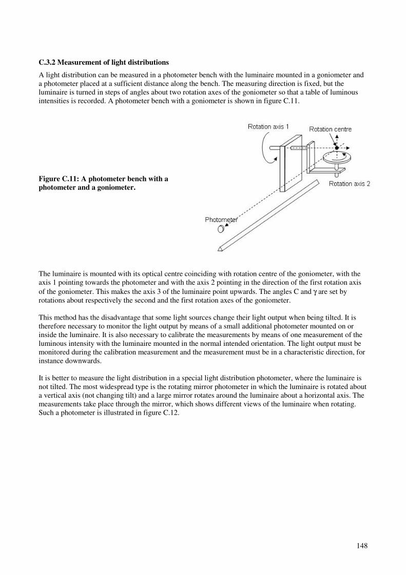
148

C.3.2 Measurement of light distributions

A light distribution can be measured in a photometer bench with the luminaire mounted in a goniometer and

a photometer placed at a sufficient distance along the bench. The measuring direction is fixed, but the

luminaire is turned in steps of angles about two rotation axes of the goniometer so that a table of luminous

intensities is recorded. A photometer bench with a goniometer is shown in figure C.11.

Figure C.11: A photometer bench with a

photometer and a goniometer.

The luminaire is mounted with its optical centre coinciding with rotation centre of the goniometer, with the

axis 1 pointing towards the photometer and with the axis 2 pointing in the direction of the first rotation axis

of the goniometer. This makes the axis 3 of the luminaire point upwards. The angles C and γ are set by

rotations about respectively the second and the first rotation axes of the goniometer.

This method has the disadvantage that some light sources change their light output when being tilted. It is

therefore necessary to monitor the light output by means of a small additional photometer mounted on or

inside the luminaire. It is also necessary to calibrate the measurements by means of one measurement of the

luminous intensity with the luminaire mounted in the normal intended orientation. The light output must be

monitored during the calibration measurement and the measurement must be in a characteristic direction, for

instance downwards.

It is better to measure the light distribution in a special light distribution photometer, where the luminaire is

not tilted. The most widespread type is the rotating mirror photometer in which the luminaire is rotated about

a vertical axis (not changing tilt) and a large mirror rotates around the luminaire about a horizontal axis. The

measurements take place through the mirror, which shows different views of the luminaire when rotating.

Such a photometer is illustrated in figure C.12.

149

Figure C.12: A rotating mirror light distribution photometer.

NOTE 1: The photo is not instructive as measurements take place in

darkness.

A rotating mirror photometer also has two rotation axis. One is vertical, about which the luminaire is rotated,

and the other is horizontal about which the mirror is rotated. The luminaire is mounted horizontally with its

optical centre in the rotation centre and its axis 3 pointing towards the photometer. The angles C and γ are set

by rotations of respectively the luminaire and the mirror.

There is a spread in the light output of individual lamps and to avoid that the measured light distribution is

affected by a particularly high or low light output, it is normal to rescale the measured light distribution to

the match the nominal light output value stated by the manufacturer of the lamp.

It therefore necessary to include a measurement of the light output of the lamp or lamps used in the luminaire

during measurement. This can be done either by measurement of the light distribution of the bare lamp(s) in

the same photometer – followed by summation of the total light output - or by measuring the light output in

an integral manner in a photometric sphere.

In the case of absolute photometry of luminaires with LED modules, there are no independent lamps to

measure. It is the responsibility of the manufacturer of the luminaires to assure that the light distribution

reflects average properties of the luminaires.

C.3.3 Orientation of luminaires in road lighting design calculations

The geometry of a road lighting installation is generally described by means of a global x, y, z co-ordinate

system. In this system, the location of a luminaire is given by its co-ordinates (x0, y0, x0). See figure C.13.

Figure C.13: The location of a luminaire as given by its co-

ordinates in a global co-ordinate system.

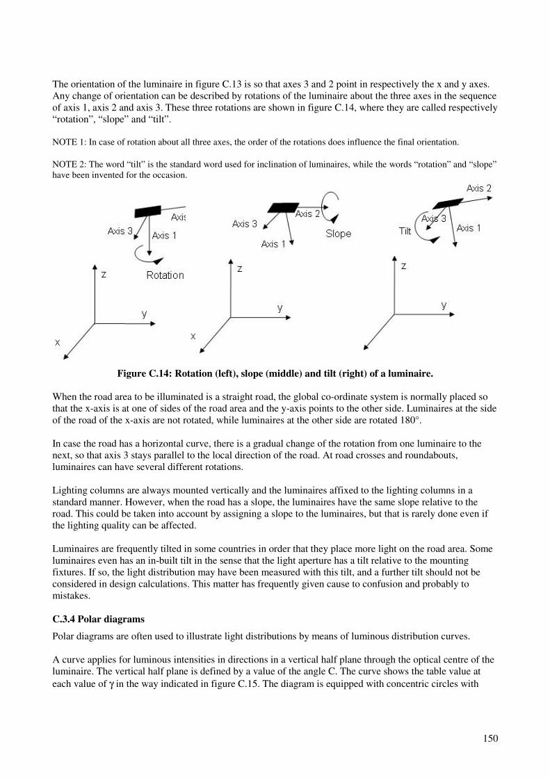
150

The orientation of the luminaire in figure C.13 is so that axes 3 and 2 point in respectively the x and y axes.

Any change of orientation can be described by rotations of the luminaire about the three axes in the sequence

of axis 1, axis 2 and axis 3. These three rotations are shown in figure C.14, where they are called respectively

“rotation”, “slope” and “tilt”.

NOTE 1: In case of rotation about all three axes, the order of the rotations does influence the final orientation. NOTE 2: The word “tilt” is the standard word used for inclination of luminaires, while the words “rotation” and “slope”

have been invented for the occasion.

Figure C.14: Rotation (left), slope (middle) and tilt (right) of a luminaire.

When the road area to be illuminated is a straight road, the global co-ordinate system is normally placed so

that the x-axis is at one of sides of the road area and the y-axis points to the other side. Luminaires at the side

of the road of the x-axis are not rotated, while luminaires at the other side are rotated 180°.

In case the road has a horizontal curve, there is a gradual change of the rotation from one luminaire to the

next, so that axis 3 stays parallel to the local direction of the road. At road crosses and roundabouts,

luminaires can have several different rotations.

Lighting columns are always mounted vertically and the luminaires affixed to the lighting columns in a

standard manner. However, when the road has a slope, the luminaires have the same slope relative to the

road. This could be taken into account by assigning a slope to the luminaires, but that is rarely done even if

the lighting quality can be affected.

Luminaires are frequently tilted in some countries in order that they place more light on the road area. Some

luminaires even has an in-built tilt in the sense that the light aperture has a tilt relative to the mounting

fixtures. If so, the light distribution may have been measured with this tilt, and a further tilt should not be

considered in design calculations. This matter has frequently given cause to confusion and probably to

mistakes.

C.3.4 Polar diagrams

Polar diagrams are often used to illustrate light distributions by means of luminous distribution curves.

A curve applies for luminous intensities in directions in a vertical half plane through the optical centre of the

luminaire. The vertical half plane is defined by a value of the angle C. The curve shows the table value at

each value of γ in the way indicated in figure C.15. The diagram is equipped with concentric circles with

151

radii that reflect steps of values, for instance 0, 50, 100, 150 and 200 cd/klm, and a set of lines through the

optical centre that reflect steps of γ, for instance 0°, 15°, 30°, 45° ... 180°.

Figure C.15: A polar diagram with a light

distribution curve.

The polar diagram of figure C.15 applies for a lantern with rotational symmetry. In this case, the actual C

value of the vertical half-plane is immaterial and the C angle is therefore not indicated. A polar diagram for

luminaires with less symmetry has often two or more light distribution curves with indications of the C-

values.

When looking at polar diagrams, it is practical that a couple of matters are understood.

One matter is that a bare lamp has a certain average value of the luminous intensity with some variation with

the direction. In case the light distribution is scaled to cd/klm, this value is 1000/(4π) = approximately 80

cd/klm. In this calculation 4π represents the total solid angle of all directions in space.

The actual luminous intensity does vary some with the direction relative to the lamp, it is for instance

approximately 100 cd/klm in a direction perpendicular to a fluorescent tube. However, it is still useful to

keep the value of 80 cd/klm in mind when judging the ability of a luminaire to direct the light. A strong

control of the directionality should lead to values of the luminous intensity that are several time 80 cd/klm in

some directions and much smaller values in other directions.

When judging the polar diagram in figure C.15 it is seen that the control of light is not strong as the

maximum luminous intensity is only 114 cd/klm. However, the light is predominantly sent downwards with

a reasonably good spread and probably also with control of glare because of low values near the horizontal.

One gets also the suspicion that the efficiency is not very high – there seems to be little or no compensation

in the lower hemisphere for the light lacking in the upper hemisphere. That is true as the efficiency is only

48,5 %.

The other matter is that the solid angle associated with a given value of γ depends on the value. The solid

angle is at a maximum at γ = 90° and decreases towards 0 at γ = 0° and at γ = 180° (the variation is actually

in proportion with sin(γ)).

152

This may lead to a wrong impression of the efficiency of a luminaire. As an example, the light distribution

curves in figure C.16 – both of rotational symmetry - correspond to the same efficiency, even if the one to

the left looks more impressive than the one to the right.

Figure C.16: Two light distribution curves corresponding to the same efficiency.

C.3.5 Examples of light distributions

Figure C.17 shows polar diagrams for an asymmetrical luminaire using parabolic optics and ellipsoidal

lamps in three different settings of the toe-in. Each of the diagrams provide light distribution curves for the

vertical half-planes of C = 0°, 15°, 30°, 45° and 90°. When the luminaire is in its normal mounting at a road,

the vertical half-plane at C = 0° is parallel to the road and the vertical half-plane at C = 90° is perpendicular

to the road.

The diagrams illustrate a good directional control of the emitted light in several respects. The efficiency is a

bit above 70 %.

The maximum luminous intensity is at or close to 400 cd/klm corresponding to 8 times the average luminous

intensity of a bare lamp. The luminous intensity is reduced somewhat at γ = 60°, but still high and

corresponds to a good reach of the beam (the light in this direction will hit the road at a distance of 1,73

times the mounting height of the luminaire). Additionally, there is a strong run-back of the luminous

intensity from γ = 60° and upwards that causes a reduction of undesirable effects of glare and intrusion of

light.

The toe-in is defined as the C angle of the vertical half-plane that contains the highest luminous intensity. It

is 25° - 30°, 30° - 35° and 35° - 40° for the diagrams A, B and C of figure C.17 respectively. This increase

in toe-in is clearly seen when comparing the diagrams.

With these three options of to-in, the luminaire should match several cases of lighting geometry with a good

result.

Figure C.18 shows polar diagrams for an asymmetrical luminaire in three different settings of the toe-in.

This luminaire uses pot optics for tubular lamps, and has an even stronger directional control of the light as

illustrated by strong beams of more than 600 cd/klm and high luminous intensities up to γ = 65° or more. The

efficiency is close to 80 %.

This luminaire can lead to a more economical lighting that the luminaire with parabolic optics, but the high

beams tend to cause more glare and intrusion of light.

153

Luminaires with LED modules can be made to have even stronger directional control of the light and may

lead to better lighting economy that with reflector optics and discharge lamps. However, consideration of

glare control and the lighting of secondary road areas set a limit to what can be achieved.

A. Small toe-in.

B. medium toe-in.

C. Large toe-in.

Figure C.17: Polar diagrams for an asymmetrical luminaire in three different settings of the toe-in.

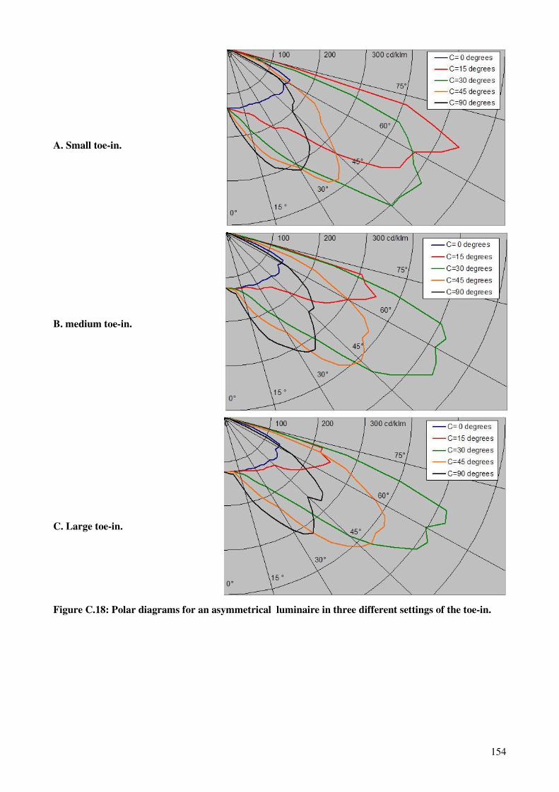
154

A. Small toe-in.

B. medium toe-in.

C. Large toe-in.

Figure C.18: Polar diagrams for an asymmetrical luminaire in three different settings of the toe-in.

155

C.4 Luminous intensity classes

Table A.1 of EN 12301-2 defines luminous intensity classes for luminaires as installed. This table is shown

in table C.1.

Table C.1: Luminous intensity classes.


Other requirements

at 70° a at 80°

a at 90°

a

G*1 200 50 None

G*2 150 30 None

G*3 100 20 None





b Luminous intensities up to 1 cd/klm can be regarded as being zero.

By luminous intensity classes for luminaires as installed is meant that the characteristic values used in table

C.1 are to be determined for the actual tilt with which the luminaire is mounted.

When a light distribution table is available for the actual tilt the procedure is as follows:

e. the luminous flux in the lower hemisphere is determined by the method of summation that has been

accounted for in C.3.1

f. this luminous flux is converted to kilolumens (klm) by division with 1000 lm/klm

g. all the values of the table are rescaled by division with the converted luminous flux

h. the rescaled values are compared to the maximum values indicated in table C.1.

In conventional photometry, the values of the light distribution table are expressed as candela per 1000

lumens of the lamp. The value determined in step a has then the unit of lm/klm while the value determined in

step b is a fraction equal to the Lower Light Output Ratio LLOR mentioned in C.3.1.

In absolute photometry used with some LED based luminaires, the values of the light distribution table are

expressed directly as candela. The value determined in step a has then the unit of lm while the value

determined in step b has the unit of klm.

When a light distribution table is available for a tilt of the luminaire that differs from the actual tilt, the

simplest thing is probably to derive a new table for the actual tilt with values that are obtained by

interpolation.

The classes G*1, G*2, G*3, G*4, G*5 and G*6 reflect increasing requirements for cut-off of the luminous

intensities at directions at the horizontal (90°), close below the horizontal (70° and 80°) or above. The

requirements are expressed by maximum proportions between the luminous intensity and the total light

output in the lower hemisphere.

156

The classes are intended for luminaires at traffic roads and are relevant for the control of glare of drivers and

also for the control of lighting nuisances such as undesirable lighting of properties, intrusions into the night

scene at long distance and illumination of the sky. It is demonstrated in the annex D that use of luminaires of

the higher classes G*4, G*5 and G*6 does ensure relatively low levels of disability glare as measured by the

Threshold Increment TI. The classes may also be applied for luminaires at domestic roads.

The classes G*1, G*2 and G*3 correspond to "semi cut-off" and "cut-off" concepts of traditional use with

requirements, however, modified to suit the prevailing use of light sources and luminaires.

Some luminaires are shown in figure C.19:

a. a luminaire with fluorescent tubes and a rather large tilt

b. a luminaire for ellipsoidal lamps with parabolic optics, a rather large tilt and a screen in the form of a

bowl

c. a luminaire as above, by with a plane glass screen and a shirt that provides some reduction of the tilt.

A: a luminaire with fluorescent tubes.

B: A luminaire with parabolic optics and a bowl.

C: A luminaire with a flat glass and a shirt.

Figure C.19: Some luminaires with weak cut-off in the classes G*1, G*2 and G*3.

The luminaires a. and b. have a weak cut-off because of the large tilts that result in rather large relative

luminous intensities in the critical directions. The bowl shaped screens of the light apertures add to the

relative luminous intensities because of reflections in the inner surfaces of the screens. These luminaires are

probably of classes G*1 or G*2.

The luminaire c has smaller relative luminous intensities in the critical directions because of the reduction of

the tilt and the avoidance of a bowl. This luminaire is probably of class G*3 or perhaps even G*4.

The classes G*4, G*5 and G*6 correspond to a strong cut-off as obtained with luminaires with little or no tilt

and flat glass screens of the light aperture.

157

Some luminaires are shown in figure C.20:

a. a luminaire with pot optics and a flat glass

b. a luminaire with an LED module and flat glass.

The luminaires a. and b. both have a strong cut-off because of avoidance of tilt. The flat glass is mostly a

hardened glass. It helps to reduce the relative luminous intensities at directions close to the horizontal

because of reduction of the transmittance due to Fresnel reflection as illustrated in figure C.21. These

luminaires correspond probably to class G*5.

A: a luminaire with pot optics and flat horizontal glass.

B: a luminaire with an LED module and flat horizontal glass.

Figure C.20: Luminaires with strong cut-off in the classes G*4, G*5 or G*6.

Figure C.21: The transmittance of a glass

plate decreases with increasing angle of

incidence due to Fresnel reflection . The

diagram applies for a refractive index of 1,55

corresponding to ordinary glass.

Transmittance of a glass plate

0

0,2

0,4

0,6

0,8

1

0 10 20 30 40 50 60 70 80 90

Angle of incidence (degrees)

Tra

ns

mit

tan

ce

158

Luminaires with a flat glass and parabolic optics for ellipsoidal lamps tend to be in the highest class of G*6,

when mounted horizontally. Luminaires with a flat glass and pot optics, on the other hand, may fail to

provide this class and fall into classes G*4 or G*5 instead.

The explanation can be sought in figure C.22 which shows the percentage projected area of a plane light

aperture at the angles of 0°, 70°, 80° and 90°. The luminous intensity at a given angle can at most equal the

product of the luminance of the lamp, the transmittance through the flat glass plate and the projected area. As

both the transmittance and the projected area decrease with the angle, the luminous intensity tends to be

fairly low and decreasing at angles of 70° and 80°. It is 0° at and above 90°.

Figure C.22: Variation of the projected area of a plane

light aperture at the angles of 0°, 70°, 80° and 90°.

This matter is relevant for luminaires with elliptical lamps and parabolic optics, as the lamps are in practice

fairly large compared to the dimensions of the light apertures. Therefore, the luminous intensities will almost

generally comply with the maximum limits for class G*6 indicated in table C.1. The luminaire, whose light

distribution is illustrated in figure C.17, is of such a type and is of class G*6.

This matter is, on the other hand, less relevant for luminaires with clear tubular lamps and pot optics. The

light aperture is small, but the luminous dimensions of the lamp are even smaller. The luminaire, whose light

distribution is illustrated in figure C.18, is of such a type and is of class G*4 only.

Therefore, with very efficient optics the use of horizontal flat glass does not ensure in itself that the cut-off is

strong. The run-back has to be supported by the optics. This applies probably for LED modules as well as pot

optics.

C.5 Glare index classes

Table A.2 of EN 12301-2 defines glare index of luminaires. This table is shown in table C.2.

Table C.2: Glare index classes

Class D0 D1 D2 D3 D4 D5 D6

Glare index maximum

– 7000 5500 4000 2000 1000 500

The glare index is I ×A-0,5

where I is the maximum value of the luminous intensity measured in candela (cd) in any direction

forming an angle of 85° from the downward vertical

and A is the apparent area in square metres (m2) of the luminous parts of the luminaire on a

plane perpendicular to the direction of I

159

The unit of the glare index is cd/m.

The value of I can be obtained from the light distribution of the luminaire. It has to be an absolute value in

candela (cd). The value of A can be derived from the luminous shape of the luminaire.

EXAMPLE 1: A luminaire with a circular horizontal light aperture of a

diameter D has an apparent area found by A = cos(85°)×π×D2/4 =

0,068×D2.

EXAMPLE 2: A luminaire with a luminous shape like a hemisphere of a

diameter D has an apparent area found by A = π×D2×(1 + cos(85°))/8 =

0,43×D2.

The classes are intended for luminaires at road areas lit for the benefit of pedestrians and pedal cyclists and are

relevant for the control of discomfort glare for these road users. Such luminaires are mostly of the lantern

type with emphasis on design and aesthetical appearance.

It is an assumption that the optics of the lantern prevent a direct view of the light source in the direction of

the luminous intensity I by means of shielding or surfaces of some diffusion or scattering. Therefore, it is a

rule that class D0 applies if parts of the light source are visible in this direction.

However, when the EN 13201 series were first drafted during the 1990’s, scepticism among some of the

participants led to the inclusion of the classes D1, D2, D3 and partly D4 of high glare index values. Bare

ellipsoidal lamps of the lower wattages would be very unpleasant in the night scene, but are nevertheless

allowed by the classes. 50 and 70 W high pressure sodium lamps fit into D2 and D1 respectively, while bare

50 and 80 W mercury lamps fit into D3 and D2 respectively.

Therefore, useful restrictions of discomfort glare are provided mainly by the classes D5 and D6.

160

The glare index is identical to a term in a “Unified Glare Rating method” that is used for indoor work places. In

the UGR method this term relates to the luminaire, while other terms relate to the position of the luminaire

relative to the line of sight and to the background level. Additionally, there is a summation for the luminaires in

the field of view. The UGR method is described in CIE 117 “Discomfort glare in interior lighting”.

The glare index represents, therefore, a strongly simplified version of the UGR method and cannot be expected

to provide an accurate impression of discomfort glare. However, the classes serve to avoid that luminaires – in

particular of the lantern type – become strongly offensive by the use of lamps of a high output compared to the

size of the luminous parts.

161

Annex X: Lighting concepts and units used for road equipment

X.1 Summary

Light, production of light and principles of light measurement are introduced in X.2. Light is electromagnetic

radiation in a narrow range of wavelengths corresponding roughly to solar radiation. Radiation with these

wavelengths acts on biological processes without being unduly harmful to life.

The concept of luminous flux is introduced. Incandescent lamps and other light sources are briefly

mentioned. Additionally, principles of light measurement are mentioned. The luminous flux is provided in

the technical documentation of light sources.

The concepts of luminous intensity and illuminance are introduced in X.3. It is pointed out that luminous

intensity relates to a direction from a lamp and is most easily understood as the ability to provide

illumination of objects or surfaces located in that direction. The illuminance is derived by means of the

distance law of illumination. Additionally, when the illuminance is to be derived for a plane that is not

perpendicular to the particular direction, the cosine law of illumination has to be taken into account as well.

The concept of luminous intensity is used in technical specifications for luminaires and signal lights.

Illuminance, on the other hand, measures the level to which a surface is illuminated and is the target for the

design of some indoor and outdoor lighting installations.

The concepts of reflection and luminance are introduced in X.4. Luminance is the stimulus for the eye. Only

objects possessing a luminance by some process (light emission, reflection or scattering) can be seen. A

particular characteristic for reflection, the luminance coefficient, represents the ability of the illuminated

surface to produce luminance.

Reflection is the subject of specifications for sign faces, road markings and other surfaces. The road surface

luminance is the target for the design of road lighting installations of traffic roads.

In X.5 it is explained that nature really works in a simple way:

- The illuminance at a location on a plane is π times the average luminance of all the objects in front of

the plane as seen from that location.

- A reflecting surface gets its luminance as an image of the surfaces in front. The luminance is normally

reduced because of absorption in the surface and there may be more emphasis to some directions than to

other directions due to shininess or other features of reflection.

Therefore, the concepts of luminous flux, luminous intensity, illuminance and reflection are not needed in

order to understand how a surface gets its luminance. However, the concepts are practical in terms of

applications by giving roles to specification writers, producers, testing laboratories and installation designers.

X.6 provides an introduction to the colour of light and of surfaces.

The concepts, units and definitions are summarized in table X.1.

It is easy to find literature on the internet. CIE 15:2004 “Colorimetry” is the bible on the rather difficult

aspects of colour.

162

Table X.1: Concepts, units and definitions.

Concept Unit Definition

Luminous flux, Φ lumen (lm) The total amount of light emitted by a light source.

Luminous intensity, I candela (cd) The density of light in a direction, or the ability to produce

illuminance on surfaces in a direction in conjunction with the laws

of illumination.

Illuminance, E lux (lx) The density of light falling on a field of a surface

Luminance, L candela/m2

(cd/m2)

The density of luminous intensity from a field of a surface.

Luminance is the stimulus for the eye.

Luminance

coefficient, q cd⋅m-2⋅lx-1

The ratio between luminance and illuminance of a field of a surface

in specified conditions of illuminance and observation.

x, y CIE Chromaticity co-ordinates.

X.2 Light, production of light and principles of light measurement

Electromagnetic radiation is characterized by its wavelength. In principle, there is no limit to the wavelength,

but in practice it may be considered to be from less than 10-10

m up to more than 100 m. Radiation within

that range is subdivided into gamma rays, X rays, ultraviolet radiation, visible radiation, infrared radiation,

radio waves and heat radiation. See figure X.1

Figure x.1:

Electromagnetic radiation and light.

Visible radiation is found at wavelengths in a narrow band about 500 nm (1 nanometer equals 10-9

m). In

principle, light is the radiant power summed up with relative weights of the so-called V(λ) curve and

multiplied by a factor of 683 lumen/Watt. The V(λ) curve represents the spectral sensitivity of the eye, while

the factor is there for historical reasons to provide a link to early definitions. The V(λ) curve is illustrated in

figure X.2.

Figure X.2: The V(λλλλ) curve representing the spectral

sensitivity of the eye (the standard observer).

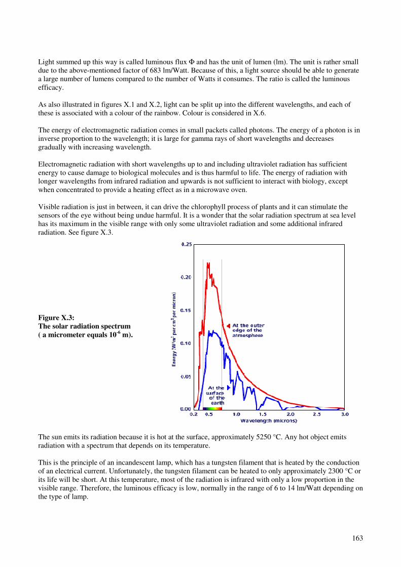
163

Light summed up this way is called luminous flux Φ and has the unit of lumen (lm). The unit is rather small

due to the above-mentioned factor of 683 lm/Watt. Because of this, a light source should be able to generate

a large number of lumens compared to the number of Watts it consumes. The ratio is called the luminous

efficacy.

As also illustrated in figures X.1 and X.2, light can be split up into the different wavelengths, and each of

these is associated with a colour of the rainbow. Colour is considered in X.6.

The energy of electromagnetic radiation comes in small packets called photons. The energy of a photon is in

inverse proportion to the wavelength; it is large for gamma rays of short wavelengths and decreases

gradually with increasing wavelength.

Electromagnetic radiation with short wavelengths up to and including ultraviolet radiation has sufficient

energy to cause damage to biological molecules and is thus harmful to life. The energy of radiation with

longer wavelengths from infrared radiation and upwards is not sufficient to interact with biology, except

when concentrated to provide a heating effect as in a microwave oven.

Visible radiation is just in between, it can drive the chlorophyll process of plants and it can stimulate the

sensors of the eye without being undue harmful. It is a wonder that the solar radiation spectrum at sea level

has its maximum in the visible range with only some ultraviolet radiation and some additional infrared

radiation. See figure X.3.

Figure X.3:

The solar radiation spectrum

( a micrometer equals 10-6

m).

The sun emits its radiation because it is hot at the surface, approximately 5250 °C. Any hot object emits

radiation with a spectrum that depends on its temperature.

This is the principle of an incandescent lamp, which has a tungsten filament that is heated by the conduction

of an electrical current. Unfortunately, the tungsten filament can be heated to only approximately 2300 °C or

its life will be short. At this temperature, most of the radiation is infrared with only a low proportion in the

visible range. Therefore, the luminous efficacy is low, normally in the range of 6 to 14 lm/Watt depending on

the type of lamp.

164

Incandescent halogen lamps has a halogen gas surrounding the filament that allows a higher temperature of

the filament and thereby a somewhat higher luminous efficacy, normally in the range of 10 to 20 lm/Watt

depending on the type of lamp.

Actually, because electromagnetic radiation is the carrier of the electromagnetic force, there are numerous

other processes for generating light than high temperature. Whenever an electron is disturbed, a quantum of

electromagnetic radiation is emitted. The practical problem is to generate electromagnetic radiation that falls

within the visible range and to allow it to leave. However, the principle is used in great variety of discharge

lamps and other light sources like light emitting diodes (LED). In some of these lamps, radiation of short

wavelengths is converted to radiation of longer wavelengths by fluorescence. Luminous efficacies are higher

than for incandescent lamps, mostly in the range of 50 to 100 lumen/Watt.

Light is measured by means of photometers. These have a photo sensitive element, mostly a photodiode,

whose spectral sensitivity has been corrected to match the V(λ) curve to an acceptable degree. The correction

is mostly by colour filters. Photometers also have suitable means to make them accept light from parts of the

space around them with defined directional sensitivity.

The luminous flux of a light source is measured in a integrating sphere that accepts light uniformly from all

directions of space. Other photometers are mentioned in the following.

The luminous flux is provided in the technical documentation of light sources.

Luminous flux is used not only in connection with light sources; it makes sense also to speak about the

luminous flux falling on a surface or a field of a surface.

X.3 Luminous intensity and illuminance

Naked light sources are sometimes used for illumination, but normally they are mounted in a lamp with

optics or shades to direct or reduce the light into specific directions.

NOTE: The word lamp is used in the following as a generic term for luminaires, lanterns, signal lights and other

lighting devices.

The lamp, therefore, modifies the directional distribution of the light emission. In each particular direction,

the intensity of light is described by a luminous intensity, I in the unit of candela (cd).

Luminous intensity has a definition of its own which, however, is complex. It is more easy to think in terms

of figure X.4, which shows a luminous surface with a luminous intensity I in a direction towards a surface

facing the luminous surface at a distance D. The luminous surface can for instance be the aperture of a

headlamp.

The concept of illuminance applies for a field of a surface. It is the ratio between the luminous flux falling on

the field and the area of the field. As the unit of luminous flux is lumen (lm), one might think that the unit of

illuminance is lumen per square meter (lm/m2). This is true, but with the modification that an individual unit

of lux (lx) has been introduced.

The luminous surface causes an illuminance E on the illuminated surface given by: E = I/D2. Accordingly,

luminous intensity can be understood as the ability to produce illuminance. The equation illustrates the

distance law of illumination - that the illuminance is in inverse proportion to the square of the distance.

EXAMPLE 1: A headlamp with a luminous intensity of 10.000 cd illuminates a surface at a distance of 50 m. The

illuminance at the surface is 10.000/502 = 4 lx.

165

Figure X.4: A luminous surface with a luminous intensity I in a direction towards an illuminated

surface at a distance D causes an illuminance of I/D2.

There is an additional law of illumination, which is to be applied when the illumination is measured on a

plane that is not perpendicular to the direction of illumination. The direction of illumination is described by

an angle of incidence v, which is shown in figure X.5. The resulting illuminance is reduced by the factor

cos(v) in accordance with the cosine law of illumination.

Figure X.5: The angle of incidence.

Consequently, the complete expression for illuminance is E = I×cos(v)/D2. Contributions from more that one

luminous surface can be summed up to a total illuminance.

Illuminance can be measured by means of a luxmeter, which is a photometer that accepts light from the

hemisphere in front of the luxmeter with a directional sensitivity in accordance with the cosine law of

illumination. A luxmeter can either be turned towards the light, or it can be placed with its back on the

surface on which the illuminance is to be measured.

A luxmeter can either be anything from a cheap handheld instrument up to an expensive laboratory

photometer.

The distance law of illumination is used for calculations of illuminance but can also be used to determine the

luminous intensity of a lamp by means of the inverse equation, I = E×D2. The illuminance E is measured by

means of a luxmeter at a known distance D and I is determined. This is the basis for laboratory measurement

of luminous intensities of lamps.

EXAMPLE 2: A headlamp produces an illuminance at 20 m distance of 25 lx. The luminous intensity is 25×20

2 =

10.000 cd.

The luminous intensity from a lamp depends generally on the direction relative to the lamp.

166

-15 -14 -13 -12 -11 -10 -9 -8 -7 -6 -5 -4 -3 -2 -1 0 1 2 3 4 5 6 7 8 9 10 11 12 13 14 15

10

9

8

7

6

5

4

3

2

1

0

horizontal angle

ve

rtic

al

an

gle

clean headlamps 375-425325-375275-325225-275175-225125-17575-12525-75

As an example, a low beam headlamp has large luminous intensities in directions below the cut-off, and

much lower luminous intensities in directions above. Refer to figure X.6, which shows the distribution of

average luminous intensity from a number of headlamps in use, after cleaning (the distribution for dirty

headlamps is broader).

Figure X.6: Average intensity distribution of some clean headlamps in use (cd).

In this example, the purpose is to provide a reasonably high illumination at some distance in front of the

vehicle without causing strong glare to oncoming traffic. Most luminaires and signal lamps have optics

designed to provide variations in the luminous intensity for similar purposes.

Therefore, it is in general necessary to measure the luminous intensity in several directions relative to the

luminaire or signal lamp. The particular set of direction is often defined in technical specifications, which in

some cases also set requirements for the luminous intensities in the individual directions.

The most common method of establishing different directions is to keep a fixed horizontal measuring

direction, but to turn the lamp in a goniometer with two axes of rotation. See figure X.7.

Figure X.7:

A lamp placed in a goniometer.

In another method, the luminaire is turned about a fixed vertical axis, while the measuring direction is varied

with respect to the horizontal by tilting a large mirror (this is not illustrated). This method takes up more

167

space, but is preferable for lamps with light sources that cannot be tilted, or light sources that changes

luminous output when tilted.

A complete table of luminous intensity values is called a luminous intensity distribution or a light

distribution. It is sometimes illustrated by means of a diagram as shown in figure X.6, and sometimes in

other ways.

The concept of luminous intensity is used in technical specifications for various luminaires and signal lights.

Illuminance is the target for the design of some indoor and outdoor lighting installations.

Luminous intensity is used not only in connection with lamps; it makes sense also to speak about the

luminous intensity emitted by reflection from a surface or a field of a surface.

X.4. Reflection and luminance

A surface that is illuminated by a lamp obtains a luminance L by reflection as seen by an observer, see figure

x.8.

Figure X.8: A surface obtains a luminance by reflection as seen by an observer.

The luminance L of a field of a surface is L = I/A, where I is the luminous intensity of the field and A is the

apparent area of the field. The luminance, the luminous intensity and the apparent area refer to a particular

observation direction. The unit for luminance is candela per square metre (cd/m2).

By apparent area of a field is meant the projection of the actual area of the field onto the direction of

observation. Refer to figure X.9.

Figure X.9: Actual and apparent area.

Luminance is the stimulus for the eye. Objects that obtain a luminance by some process (light emission,

reflection or scattering) can be seen, light as such cannot.

Luminance is measured by means of a photometer called a luminance meter, which has optics to allow light

only from a field confined by a small cone. The size of the cone is measured by its angular diameter, which

may typically be 6’, 20’, 1° or 3°. The field confined by the cone is called the measuring field.

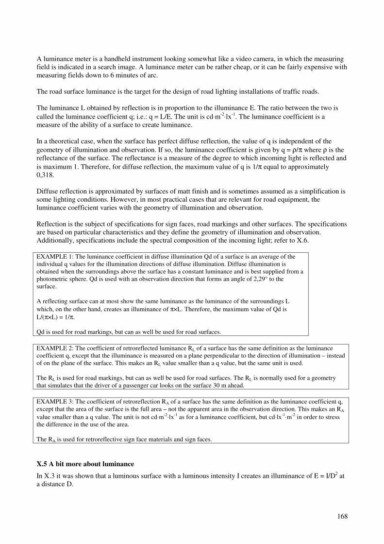
168

A luminance meter is a handheld instrument looking somewhat like a video camera, in which the measuring

field is indicated in a search image. A luminance meter can be rather cheap, or it can be fairly expensive with

measuring fields down to 6 minutes of arc.

The road surface luminance is the target for the design of road lighting installations of traffic roads.

The luminance L obtained by reflection is in proportion to the illuminance E. The ratio between the two is

called the luminance coefficient q; i.e.: q = L/E. The unit is cd⋅m-2⋅lx-1. The luminance coefficient is a

measure of the ability of a surface to create luminance.

In a theoretical case, when the surface has perfect diffuse reflection, the value of q is independent of the

geometry of illumination and observation. If so, the luminance coefficient is given by q = ρ/π where ρ is the

reflectance of the surface. The reflectance is a measure of the degree to which incoming light is reflected and

is maximum 1. Therefore, for diffuse reflection, the maximum value of q is 1/π equal to approximately

0,318.

Diffuse reflection is approximated by surfaces of matt finish and is sometimes assumed as a simplification is

some lighting conditions. However, in most practical cases that are relevant for road equipment, the

luminance coefficient varies with the geometry of illumination and observation.

Reflection is the subject of specifications for sign faces, road markings and other surfaces. The specifications

are based on particular characteristics and they define the geometry of illumination and observation.

Additionally, specifications include the spectral composition of the incoming light; refer to X.6.

EXAMPLE 1: The luminance coefficient in diffuse illumination Qd of a surface is an average of the

individual q values for the illumination directions of diffuse illumination. Diffuse illumination is

obtained when the surroundings above the surface has a constant luminance and is best supplied from a

photometric sphere. Qd is used with an observation direction that forms an angle of 2,29° to the

surface.

A reflecting surface can at most show the same luminance as the luminance of the surroundings L

which, on the other hand, creates an illuminance of π×L. Therefore, the maximum value of Qd is

L/(π×L) = 1/π.

Qd is used for road markings, but can as well be used for road surfaces.

EXAMPLE 2: The coefficient of retroreflected luminance RL of a surface has the same definition as the luminance

coefficient q, except that the illuminance is measured on a plane perpendicular to the direction of illumination – instead

of on the plane of the surface. This makes an RL value smaller than a q value, but the same unit is used.

The RL is used for road markings, but can as well be used for road surfaces. The RL is normally used for a geometry

that simulates that the driver of a passenger car looks on the surface 30 m ahead.

EXAMPLE 3: The coefficient of retroreflection RA of a surface has the same definition as the luminance coefficient q,

except that the area of the surface is the full area – not the apparent area in the observation direction. This makes an RA

value smaller than a q value. The unit is not cd⋅m-2⋅lx-1 as for a luminance coefficient, but cd⋅lx-1⋅m-2

in order to stress

the difference in the use of the area.

The RA is used for retroreflective sign face materials and sign faces.

X.5 A bit more about luminance

In X.3 it was shown that a luminous surface with a luminous intensity I creates an illuminance of E = I/D2 at

a distance D.

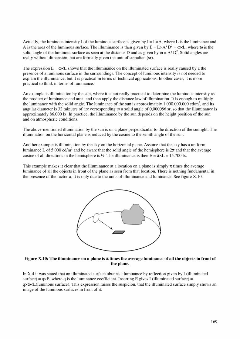
169

Actually, the luminous intensity I of the luminous surface is given by I = L×A, where L is the luminance and

A is the area of the luminous surface. The illuminance is then given by E = L×A/ D2 = ω×L, where ω is the

solid angle of the luminous surface as seen at the distance D and as given by ω = A/ D2. Solid angles are

really without dimension, but are formally given the unit of steradian (sr).

The expression E = ω×L shows that the illuminance on the illuminated surface is really caused by a the

presence of a luminous surface in the surroundings. The concept of luminous intensity is not needed to

explain the illuminance, but it is practical in terms of technical applications. In other cases, it is more

practical to think in terms of luminance.

An example is illumination by the sun, where it is not really practical to determine the luminous intensity as

the product of luminance and area, and then apply the distance law of illumination. It is enough to multiply

the luminance with the solid angle. The luminance of the sun is approximately 1.000.000.000 cd/m2, and its

angular diameter is 32 minutes of arc corresponding to a solid angle of 0,000086 sr, so that the illuminance is

approximately 86.000 lx. In practice, the illuminance by the sun depends on the height position of the sun

and on atmospheric conditions.

The above-mentioned illumination by the sun is on a plane perpendicular to the direction of the sunlight. The

illumination on the horizontal plane is reduced by the cosine to the zenith angle of the sun.

Another example is illumination by the sky on the horizontal plane. Assume that the sky has a uniform

luminance L of 5.000 cd/m2 and be aware that the solid angle of the hemisphere is 2π and that the average

cosine of all directions in the hemisphere is ½. The illuminance is then E = π×L = 15.700 lx.

This example makes it clear that the illuminance at a location on a plane is simply π times the average

luminance of all the objects in front of the plane as seen from that location. There is nothing fundamental in

the presence of the factor π, it is only due to the units of illuminance and luminance. See figure X.10.

Figure X.10: The illuminance on a plane is ππππ times the average luminance of all the objects in front of

the plane.

In X.4 it was stated that an illuminated surface obtains a luminance by reflection given by L(illuminated

surface) = q×E, where q is the luminance coefficient. Inserting E gives L(illuminated surface) =

q×ω×L(luminous surface). This expression raises the suspicion, that the illuminated surface simply shows an

image of the luminous surfaces in front of it.

170

This is true. A reflecting surface gets its luminance as an image of the surfaces in front. The luminance may

be reduced because of absorption in the surface and there may be more emphasis to some directions than to

other directions due to shininess or other features of reflection. The image is mostly diffused or blurred

depending on the properties of the reflecting surface.

As an example, a road surface with a reflectance of 0,25 under a uniform sky has a luminance 0,25 times the

sky luminance.

Therefore, the concepts of illuminance and luminance coefficient are not really needed in order to explain

how an illuminated surface gets a luminance, but the concepts are practical for technical applications.

X.6 Colour of light and surfaces

The CIE 1931 colour space is the most widely used colour system for technical specifications of colours.

The tri-stimuli values X, Y and Z are found as weighted summations of the spectral radiant power. The

weights are in accordance with the curves x(λ), y(λ) and z(λ) indicated in figure X.11. The curve y(λ) is

actually the same curve as the V(λ) and appears in this connection with a different designation only.

Figure X.11: The curves x(λλλλ), y(λλλλ) and z(λλλλ) used to derive the tri-stimuli values X, Y and Z.

The two chromaticity co-ordinates x and y are found by x = X/(X+Y+Z) and y = Y/(X+Y+Z). Those two co-

ordinates determine a location in the CIE chromaticity diagram shown in figure X.12. The numbers indicated

around the curving part of the triangular colour region refer to the wavelengths of light of a single

wavelength, i.e. to the colours of the rainbow. The curving part is called the spectrum locus. All other

colours are mixtures of these colours.

Permissible colours of signal lights are generally indicated by colour regions or colour boxes in the

chromaticity diagram.

Colours of light of light sources are indicated in similar ways or with reference to a curve for temperature

radiators by means of a correlated colour temperature (this curve is not indicated in figure X.12).

Permissible colours of reflecting surfaces are also indicated by colour boxes in the chromaticity diagram.

The surfaces represent for instance sign faces or road markings. However, the chromaticity of a reflecting

surface depends on the illuminant used to illuminate the surface and on the geometry of illumination and

observation. These matters are therefore specified and lie behind the requirements. The value of Y has a

meaning as a measure of the reflection.

171

Chromaticity boxes for retroreflective sheeting

materials

0

0,1

0,2

0,3

0,4

0,5

0,6

0,7

0,8

0,9

0 0,1 0,2 0,3 0,4 0,5 0,6 0,7 0,8 x

y

white and greyyelloworangeredbluegreendark greenbrownpurple

The illuminants are generally standard illuminant A, which represents a headlamp with an incandescent

lamp, or standard illuminant D65, which represents daylight. The most used geometry of illumination and

observation is the 45°/0° geometry. The value of Y is mostly in the scale of a luminance factor, which is π

times the scale of a luminance coefficient.

As an example, the chromaticity boxes of retroreflective sheeting materials are shown in figure X.13. These

apply for standard illuminant D65 and the 45°/0° geometry. The boxes include only non-fluorescent

materials, as fluorescent materials have separate boxes.

Figure X.12: The CIE chromaticity diagram.

Figure X.13:

Example of colour boxes.

NOTE: The sizes of the colour boxes do not necessarily indicate the permissible variations of colour within the boxes,

as the distances in figures X.12 and X.13 do not indicate degrees of visual distances.

Literature

CIE 15, Colorimetry, 2004

Documents

Road lighting Foreword - nmfv.dk · road lighting and provided recommendations for the lighting levels to use on different roads. The attitude is that the experts are the only ones