Road Density as an Indicator of Road Hazard - US Forest Service

165

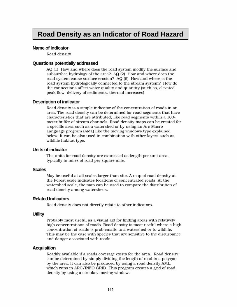
Road Density as an Indicator of Road Hazard

Name of indicatorRoad density

Questions potentially addressedAQ (1) How and where does the road system modify the surface andsubsurface hydrology of the area? AQ (2) How and where does theroad system cause surface erosion? AQ (6) How and where is theroad system hydrologically connected to the stream system? How dothe connections affect water quality and quantity (such as, elevatedpeak flow, delivery of sediments, thermal increases)

Description of indicatorRoad density is a simple indicator of the concentration of roads in anarea. The road density can be determined for road segments that havecharacteristics that are attributed, like road segments within a 100-meter buffer of stream channels. Road density maps can be created fora specific area such as a watershed or by using an Arc MacroLanguage program (AML) like the moving windows type explainedbelow. It can be also used in combination with other layers such aswildlife habitat type.

Units of indicatorThe units for road density are expressed as length per unit area,typically in miles of road per square mile.

ScalesMay be useful at all scales larger than site. A map of road density atthe Forest scale indicates locations of concentrated roads. At thewatershed scale, the map can be used to compare the distribution ofroad density among watersheds.

Related IndicatorsRoad density does not directly relate to other indicators.

UtilityProbably most useful as a visual aid for finding areas with relativelyhigh concentrations of roads. Road density is most useful where a highconcentration of roads is problematic to a watershed or to wildlife.This may be the case with species that are sensitive to the disturbanceand danger associated with roads.

AcquisitionReadily available if a roads coverage exists for the area. Road densitycan be determined by simply dividing the length of road in a polygonby the area. It can also be produced by using a road density AML,which runs in ARC/INFO GRID. This program creates a grid of roaddensity by using a circular, moving window.

166

Data needsMust have a roads coverage for the GIS process. Road density bywatershed can be done manually by determining the length of roadsand dividing by the area.

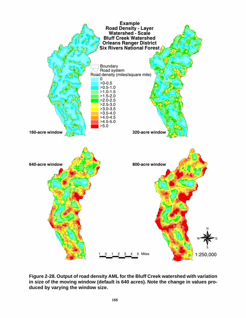
Accuracy and precisionThis macro can produce very different results (figure 2-28), dependingon the window size selected. The default setting for the window size is1 square mile. The default setting for the cell size is 1 acre. Setting thewindow size less than the default will lower the density values on theroad-density map because the moving window is less likely to overlapthe adjacent roads. Reducing the cell size will smooth the polygonoutput but will add processing time. If the input roads coverage doesnot extend beyond the cover used to clip the output coverage, it maynot be accurate around the perimeter.

DurabilityWill change over time if roads are dropped or added to the roadscoverage.

Monitoring valueCan be useful if a resource responds to a threshold value of roaddensity.

LimitationsRoad density may not be appropriate for some analyses because itdoes not reflect the character of individual roads. In some watersheds,the aquatic effects from a single problem road will be greater than inan area with high road density. This macro is very sensitive to the sizeof moving window selected. The roads coverage must extend beyondthe boundary, if the road density along the perimeter is to be accurate.

Typical availabilityWherever a digital roads coverage exists. Road density can bedetermined manually for an area such as a watershed or district, butit would be very tedious to manually recreate the moving windowsAML.

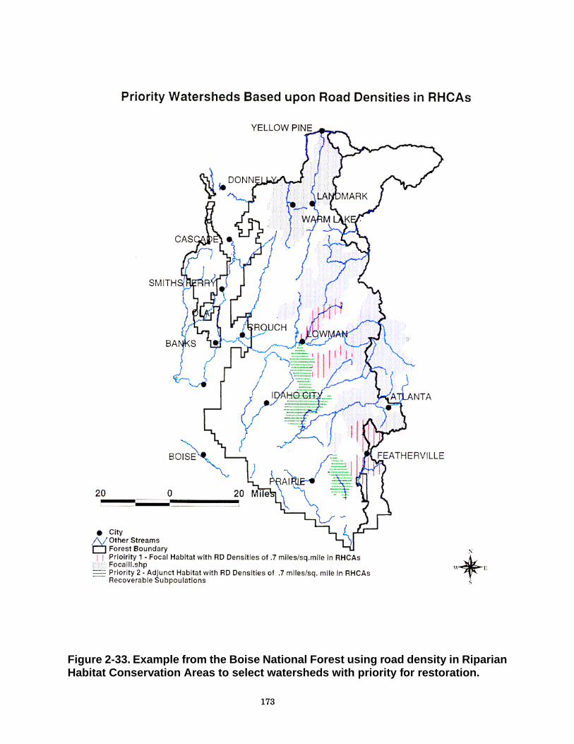
Where applicableRoad density is probably best applied in combination with a polygoncoverage. An example of a combination is road density in riparianreserves (figure 2-33).

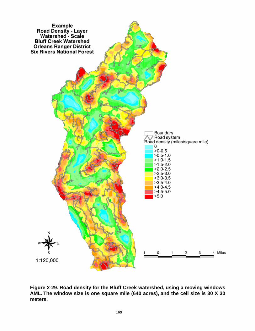
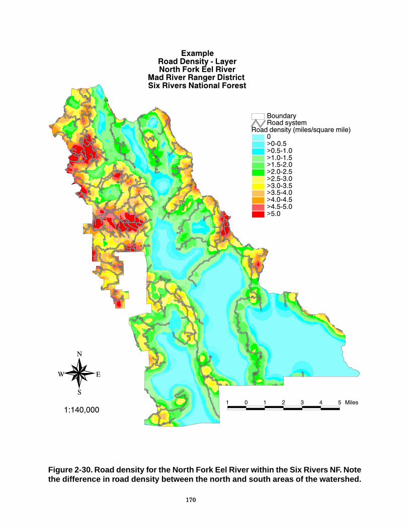
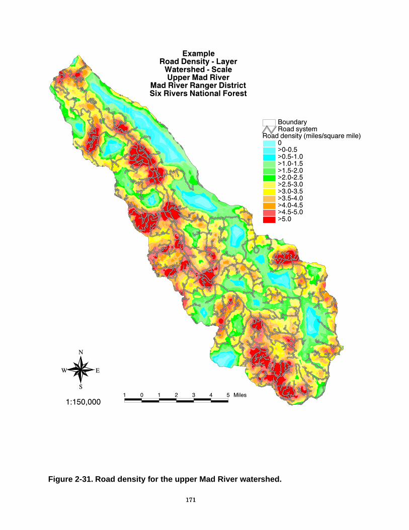
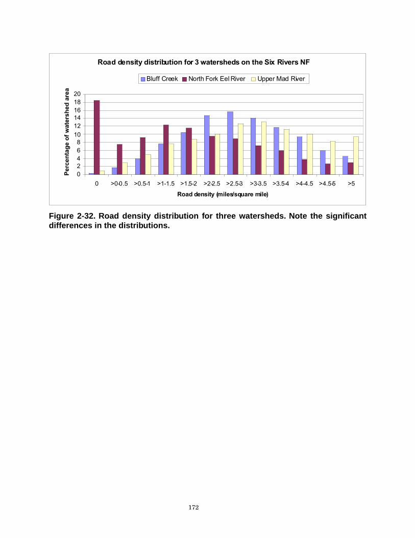
ExamplesRoad density was calculated for three watersheds (figures 2-29, -30, -31) on the Six Rivers NF, by using the default moving-window size ofone square mile and a cell size of 30 X 30 meters (default is 1 acre orabout 64 X 64 meters). The distribution of road density (figure 2-32)shows the Bluff Creek watershed with a fairly normal distribution. TheNorth Fork Eel river road density has more than 18 percent of its areain the zero category because of the two wilderness areas in the

167

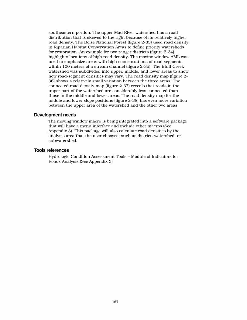
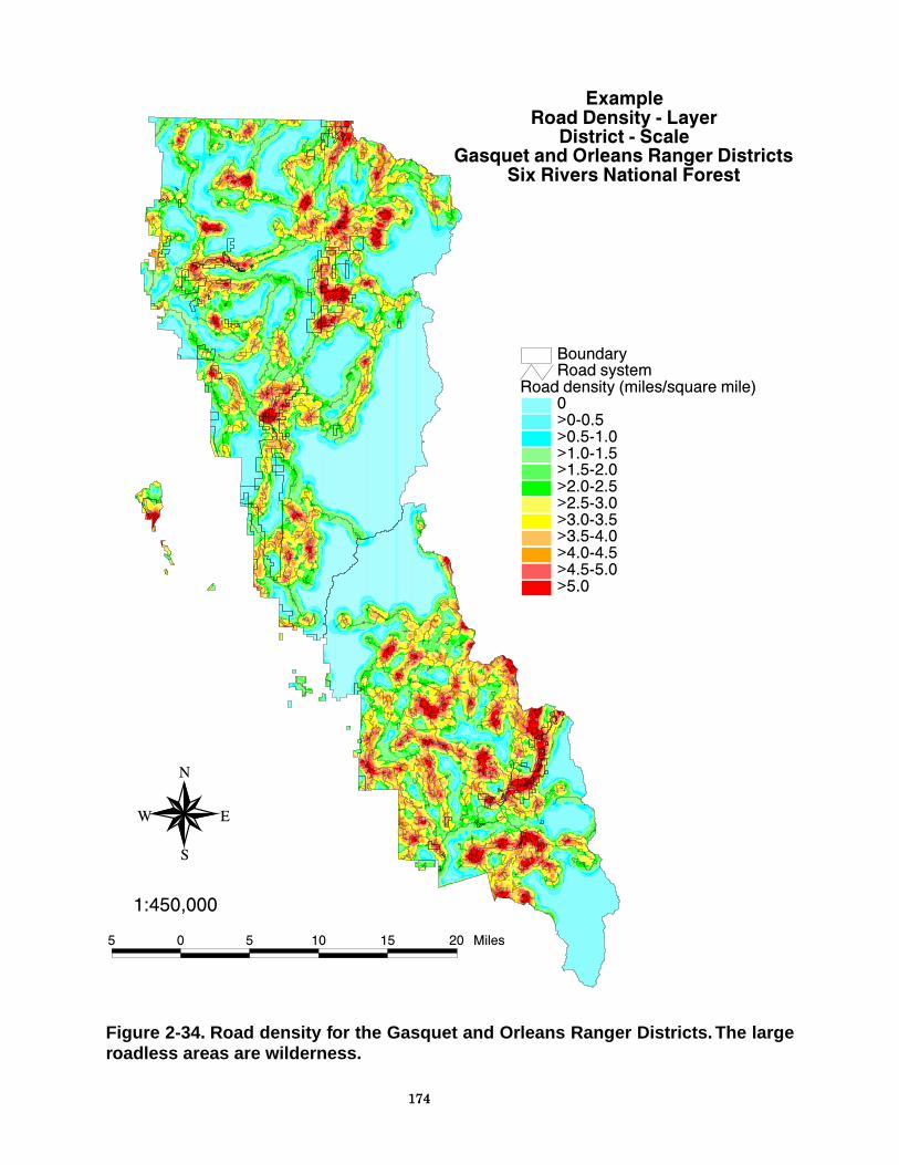
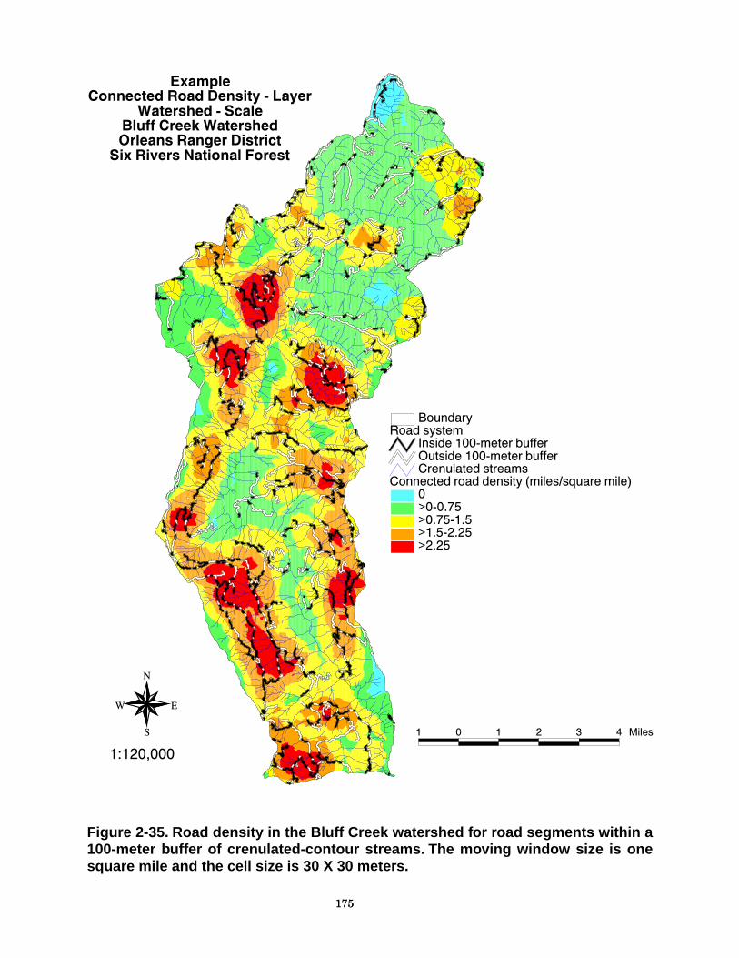
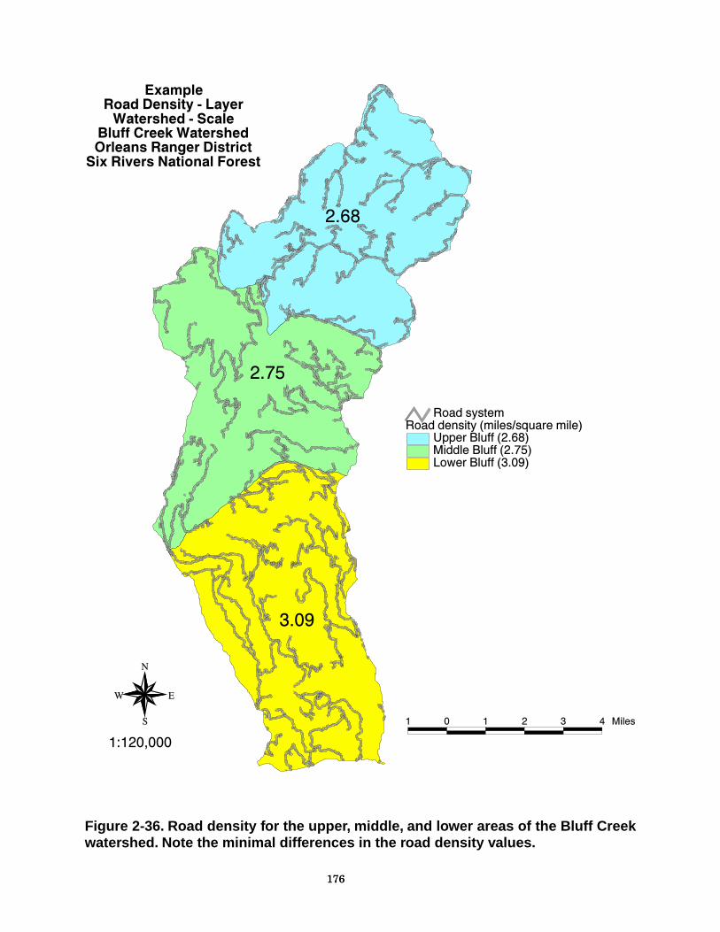
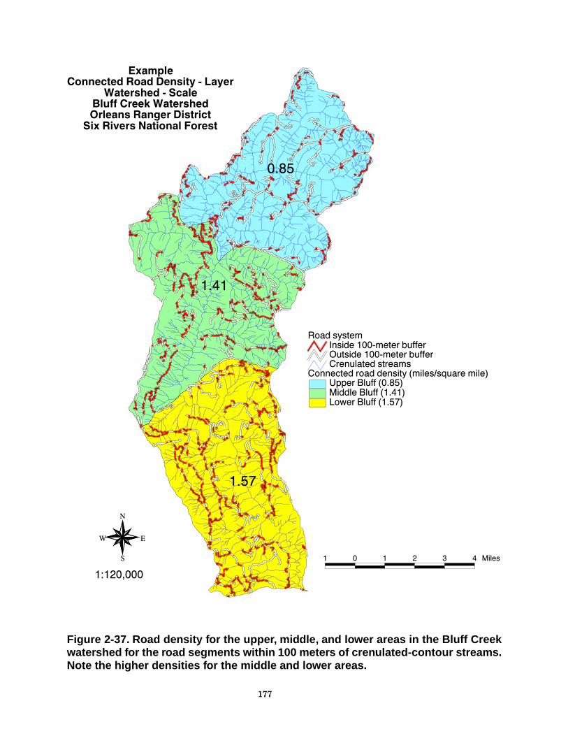
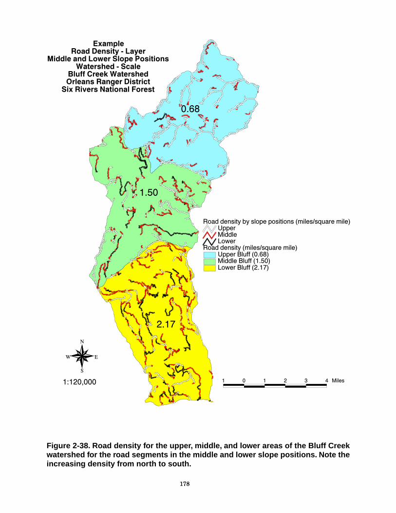
southeastern portion. The upper Mad River watershed has a roaddistribution that is skewed to the right because of its relatively higherroad density. The Boise National Forest (figure 2-33) used road densityin Riparian Habitat Conservation Areas to define priority watershedsfor restoration. An example for two ranger districts (figure 2-34)highlights locations of high road density. The moving window AML wasused to emphasize areas with high concentrations of road segmentswithin 100 meters of a stream channel (figure 2-35). The Bluff Creekwatershed was subdivided into upper, middle, and lower areas to showhow road-segment densities may vary. The road density map (figure 2-36) shows a relatively small variation between the three areas. Theconnected road density map (figure 2-37) reveals that roads in theupper part of the watershed are considerably less connected thanthose in the middle and lower areas. The road density map for themiddle and lower slope positions (figure 2-38) has even more variationbetween the upper area of the watershed and the other two areas.

Development needsThe moving window macro is being integrated into a software packagethat will have a menu interface and include other macros (SeeAppendix 3). This package will also calculate road densities by theanalysis area that the user chooses, such as district, watershed, orsubwatershed.

Tools referencesHydrologic Condition Assessment Tools – Module of Indicators forRoads Analysis (See Appendix 3)

168

N

EW

S

ExampleRoad Density - Layer

Watershed - ScaleBluff Creek WatershedOrleans Ranger District

Six Rivers National Forest

1 0 1 2 3 4 5 Miles

160-acre window 320-acre window

640-acre window 800-acre window

1:250,000

Road density (miles/square mile)0>0-0.5 >0.5-1.0>1.0-1.5 >1.5-2.0>2.0-2.5 >2.5-3.0>3.0-3.5 >3.5-4.0>4.0-4.5 >4.5-5.0>5.0

Road systemBoundary

Figure 2-28. Output of road density AML for the Bluff Creek watershed with variationin size of the moving window (default is 640 acres). Note the change in values pro-duced by varying the window size.

168

169


Road systemBoundary

N

EW

S

1:120,000




1 0 1 2 3 4 Miles

Figure 2-29. Road density for the Bluff Creek watershed, using a moving windowsAML. The window size is one square mile (640 acres), and the cell size is 30 X 30meters.

169

170


Road systemBoundary

N

EW

S1 0 1 2 3 4 5 Miles

1:140,000

ExampleRoad Density - LayerNorth Fork Eel River

Mad River Ranger District Six Rivers National Forest

Figure 2-30. Road density for the North Fork Eel River within the Six Rivers NF. Notethe difference in road density between the north and south areas of the watershed.

170

171


Road systemBoundary


Watershed - ScaleUpper Mad River

Mad River Ranger DistrictSix Rivers National Forest

N

EW

S1 0 1 2 3 4 5 Miles

1:150,000

Figure 2-31. Road density for the upper Mad River watershed.

171

172

Figure 2-32. Road density distribution for three watersheds. Note the significantdifferences in the distributions.

Road density distribution for 3 watersheds on the Six Rivers NF

0

2

4

6

8

10

12

14

16

18

20

0 >0-0.5 >0.5-1 >1-1.5 >1.5-2 >2-2.5 >2.5-3 >3-3.5 >3.5-4 >4-4.5 >4.5-5 >5

Road density (miles/square mile)

Perc

en

tag

e o

f w

ate

rsh

ed

are

a

Bluff Creek North Fork Eel River Upper Mad River

173

Figure 2-33. Example from the Boise National Forest using road density in RiparianHabitat Conservation Areas to select watersheds with priority for restoration.

173

174


Road systemBoundary


District - ScaleGasquet and Orleans Ranger Districts


N

EW

S

5 0 5 10 15 20 Miles

1:450,000

Figure 2-34. Road density for the Gasquet and Orleans Ranger Districts. The largeroadless areas are wilderness.

174

175

Connected road density (miles/square mile)0>0-0.75>0.75-1.5>1.5-2.25>2.25

Crenulated streams

Road systemInside 100-meter bufferOutside 100-meter buffer

Boundary

N

EW

S

1:120,000

ExampleConnected Road Density - Layer



1 0 1 2 3 4 Miles

Figure 2-35. Road density in the Bluff Creek watershed for road segments within a100-meter buffer of crenulated-contour streams. The moving window size is onesquare mile and the cell size is 30 X 30 meters.

175

176

3.09

2.75

2.68

Road density (miles/square mile)Upper Bluff (2.68)Middle Bluff (2.75)Lower Bluff (3.09)

Road system

N

EW

S

1:120,000




1 0 1 2 3 4 Miles

Figure 2-36. Road density for the upper, middle, and lower areas of the Bluff Creekwatershed. Note the minimal differences in the road density values.

176

177

1.57

1.41

0.85

Connected road density (miles/square mile)Upper Bluff (0.85)Middle Bluff (1.41)Lower Bluff (1.57)

Crenulated streams

Road systemInside 100-meter bufferOutside 100-meter buffer

N

EW

S

1:120,000

ExampleConnected Road Density - Layer



1 0 1 2 3 4 Miles

Figure 2-37. Road density for the upper, middle, and lower areas in the Bluff Creekwatershed for the road segments within 100 meters of crenulated-contour streams.Note the higher densities for the middle and lower areas.

177

178

2.17

1.50

0.68

Road density (miles/square mile)Upper Bluff (0.68)Middle Bluff (1.50)Lower Bluff (2.17)

Road density by slope positions (miles/square mile)UpperMiddleLower

N

EW

S

1:120,000


Middle and Lower Slope PositionsWatershed - Scale

Bluff Creek WatershedOrleans Ranger District


1 0 1 2 3 4 Miles

Figure 2-38. Road density for the upper, middle, and lower areas of the Bluff Creekwatershed for the road segments in the middle and lower slope positions. Note theincreasing density from north to south.

178

Documents

Road Density as an Indicator of Road Hazard - US Forest Service