RIVER RESEARCH AND APPLICATIONS APPLICATION OF A 2D

Uncor

recte

d Pr

oof

Uncor

recte

d Pr

oof

RIVER RESEARCH AND APPLICATIONS

River Res. Applic. 19: 1–21 (2003)

Published online in Wiley InterScience(www.interscience.wiley.com). DOI: 10.1002/rra.748

APPLICATION OF A 2D HYDRODYNAMIC MODEL TO DESIGN OFREACH-SCALE SPAWNING GRAVEL REPLENISHMENT ON THE

MOKELUMNE RIVER, CALIFORNIA

GREGORY B. PASTERNACK,a* C. LAU WANGa and JOSEPH MERZb

a Department of Land, Air, and Water Resources, University of California, 1 Shields Avenue, Davis, CA 95616-8626, USAb East Bay Municipal Utility District, 1 Winemasters Way, Lodi, CA 95240, USA

ABSTRACT

In-stream chinook salmon (Oncorhynchus tschawytscha) spawning habitat in California’s Central Valley has been degraded byminimal gravel recruitment due to river impoundment and historic gravel extraction. In a recent project marking a new directionfor spawning habitat rehabilitation, 2450 m3 of gravel and several boulders were used to craft bars and chutes. To improve thedesign of future projects, a test was carried out in which a commercial modelling package was used to design and evaluatealternative gravel configurations in relation to the actual pre- and post-project configurations. Tested scenarios included alter-nate bars, central braid, a combination of alternate bars and a braid, and a flat riffle with uniformly spaced boulders. All runswere compared for their spawning habitat value and for susceptibility to erosion. The flat riffle scenario produced the most total,high, and medium quality habitat, but would yield little habitat under flows deviating from the design discharge. Bar and braidscenarios were highly gravel efficient, with nearly 1 m2 of habitat per 1 m3 of gravel added, and yielded large contiguous highquality habitat patches that were superior to the actual design. At near bankfull flow, negligible sediment entrainment was pre-dicted for any scenario. Copyright # 2003 John Wiley & Sons, Ltd.

key words: river restoration; 2D modelling; salmon; gravel; numerical modelling; salmon spawning; physical habitat

INTRODUCTION

In California salmonid spawning habitat has been degraded or depleted by a plethora of instream human activities

and upland land uses (Nehlsen et al., 1991; Moyle and Randall, 1998; Yoshiyama et al., 1998). Dam construction

and operation (Kondolf, 1997; Brandt, 2000), gravel extraction (Gilvear et al., 1995; Kondolf et al., 1996), historic

gold mining (Harvey and Lisle, 1998), channelization (Nagasaka and Nakamura, 1999), water diversion (Petts,

1996; Douglas and Taylor, 1998), deforestation (Platts and Megahan, 1975; Marks and Rutt, 1997), and intensive

agriculture (Soulsby et al., 2000) are specific activities that disrupt healthy stream ecology (Allan and Flecker,

1993; Poff et al., 1997). While California’s commercial landings of chinook salmon (Oncorhynchus tschawytscha)

show wide annual variability, a consistent downward trend in decadal harvest during 1950–2000 from 33 621 to

18 980 tonnes indicates a serious threat to species survival (National Marine Fisheries Service, 2001).

For Sierra Nevada streams, dams prevent salmon from reaching historic spawning sites (Moyle and Randall,

1998). Spawning areas below the lowest impassable dams are now critical to survival of seasonal runs. As a result,

maintenance flows are provided during different spawning seasons (Castleberry et al., 1996; Moyle et al., 1998).

However, even with a minimal flow regime in place, spawning areas below dams suffer gravel losses in winter

floods, have little gravel recruitment, and experience channel changes. Thus, dams have altered flow regimes

and created out-of-balance sediment budgets that hurt chinook salmon populations.

Received 11 April 2002

Revised 26 November 2002

Copyright # 2003 John Wiley & Sons, Ltd. Accepted 9 December 2002

* Correspondence to: Gregory B. Pasternack, Department of Land, Air, and Water Resources, University of California, 1 Shields Avenue, Davis,CA 95616-8626, USA. E-mail: [email protected]

1

2

3

4

5

6

7

8

9

10

11

12

13

14

15

16

17

18

19

20

21

22

23

24

25

26

27

28

29

30

31

32

33

34

35

36

37

38

39

40

41

42

43

44

45

46

47

48

49

50

51

52

53

54

55

56

57

58

59

60

61

62

63

64

65

1

2

3

4

5

6

7

8

9

10

11

12

13

14

15

16

17

18

19

20

21

22

23

24

25

26

27

28

29

30

31

32

33

34

35

36

37

38

39

40

41

42

43

44

45

46

47

48

49

50

51

52

53

54

55

56

57

58

59

60

61

62

63

64

65

Uncor

recte

d Pr

oof

Uncor

recte

d Pr

oof

Instream mining has exacerbated the problem by severely depleting available gravel. Mining alters channel geo-

metry and elevation, and involves extensive clearing, flow diversion, sediment stockpiling, and deep pit excavation

(Sandecki, 1989). Tens to hundreds of millions of tons of gravel are being removed from California’s rivers creat-

ing a serious gravel deficit.

Gravel replenishment projects had been undertaken to mitigate severely degraded spawning areas below Sierra

Nevada dams in more than 13 rivers in California as of 1992 (Kondolf and Matthews, 1993). The largest of these

efforts is on the Upper Sacramento River where gravel replenishment has been conducted from 1979 to 2002.

Gravel replenishment has been used to raise beds to pre-regulation elevations, prevent channel incision, and in

rare cases to create features such as islands and pool–riffle sequences.

Even though these projects may provide some short-term habitat, the amount of gravel added is a small fraction

of the bedload deficit. Gravels placed in the main channel have washed downstream during high flows, requiring

continued addition of more imported gravel (California Department of Water Resources, 1995). Also, few objec-

tive criteria exist for designing and placing in-channel features. Project failure often results from a lack of under-

standing of geomorphic processes. In many cases designs have been based on ‘folklore’ or aesthetic criteria rather

than application of hydrology and hydrodynamics (National Research Council, 1992).

Post-construction monitoring of gravel replenishment in California has been limited. One exception was a study

of the Merced, Tuolumne, and Stanislaus rivers (Kondolf et al., 1996). Ten sites were excavated and back-filled

with smaller gravel to create spawning habitat for chinook salmon from 1990 to 1994, but placed gravel sizes were

mobile at high flows recurring at 1.5–4 year intervals. Channel surveys showed that augmented gravels washed out.

Based on limited assessment and uncertain success of gravel projects to date, it is apparent that current strategies

are not yielding optimal usable habitat while minimizing gravel losses by flow-induced sediment entrainment. The

goal of this study was to test the applicability of a commercial modelling package with a two-dimensional (2D)

hydrodynamic model for use in designing fine-scale gravel placement to rehabilitate and augment salmon spawn-

ing habitat as well as to reintroduce fluvial complexity. 2D hydrodynamic models quantify depth, velocity, and

shear stress at ecologically relevant scales, such as a pool–riffle reach or in the vicinity of a single boulder. When

model output is coupled with quantitative estimates of preferred physical habitat conditions, the result is a power-

ful tool for characterizing instream habitat (Leclerc et al., 1995). If this tool could be used prescriptively, then

many potential alternative scenarios could be assessed for habitat quality and geomorphic sustainability prior to

project construction.

The test site for this study was a gravel project by the East Bay Municipal Utility District (EBMUD) on the

Mokelumne River downstream of Camanche Dam in the Central Valley, California (Figure 1). Commercial soft-

ware was used to build and compare alternative scenarios with actual pre- and post-project conditions. Habitat

suitability indices assessed low-flow chinook salmon spawning habitat, while a sediment mobility index predicted

entrainment at near-bankfull discharge. Specific objectives were to: (1) build and analyse 2D models of an alluvial

reach before and after gravel replenishment; (2) create four alternative design scenarios—alternate bars, channel

braid, alternate barsþ braid, and flat with boulders; and (3) compare the pre- and post-project hydrodynamic, habi-

tat, and geomorphic conditions with those of the alternative scenarios. This study provides lessons for future

gravel-bar design worldwide.

ECOLOGICAL APPLICATION OF HYDRODYNAMIC MODELS

2D models using depth-averaged Saint-Venant equations are increasingly used for aquatic biology and geomor-

phology. Their primary advantage over 1D models (e.g. HEC-2 and MIKE-11) for these applications is that they

yield fine-scale distributions of velocity vectors (including lateral components) as opposed to ecologically and

geomorphically insignificant cross-sectional average downstream speeds. Nodal velocity vectors can be used to

estimate local habitat and shear stress conditions. It is very well known that the trade-off for this improvement

is the expense of pre-project fine-scale field mapping because the quality of model results is strongly dependent

upon the accuracy and spatial resolution of the underlying topographic and parameter measurements as well as the

resultant digital elevation model (Leclerc et al., 1995; Ghanem et al., 1996). Most 2D models assume a hydrostatic

pressure distribution and are thus incapable of handling substantial vertical accelerations or bed gradients >0.10

(Miller and Cluer, 1999). Lane et al. (1999) evaluated the extent 3D models improved predictive ability over 2D

2 G. B. PASTERNACK, C. L. WANG AND J. MERZ

Copyright # 2003 John Wiley & Sons, Ltd. River Res. Applic. 19: 1–21 (2003)

1

2

3

4

5

6

7

8

9

10

11

12

13

14

15

16

17

18

19

20

21

22

23

24

25

26

27

28

29

30

31

32

33

34

35

36

37

38

39

40

41

42

43

44

45

46

47

48

49

50

51

52

53

54

55

56

57

58

59

60

61

62

63

64

65

1

2

3

4

5

6

7

8

9

10

11

12

13

14

15

16

17

18

19

20

21

22

23

24

25

26

27

28

29

30

31

32

33

34

35

36

37

38

39

40

41

42

43

44

45

46

47

48

49

50

51

52

53

54

55

56

57

58

59

60

61

62

63

64

65

Uncor

recte

d Pr

oof

Uncor

recte

d Pr

oof

ones. They reported an extreme non-linear sensitivity in 3D models to minor variations in bed geometry and chan-

nel network, thus yielding dramatically different flow predictions and bed shear stresses. Given the limits of tech-

nology to get field data to calibrate and validate 3D models at the necessary sub-reach scale, 2D models are now the

most promising tools for gravel replenishment.

Crowder and Diplas (2000) showed that 2D models can simulate sub-reach-scale stream features with ecological

relevance. Small obstructions create velocity gradients, velocity shelters, transverse flows, etc. that were not evi-

dent when the obstructions were omitted from their model. Geomorphic applications of 2D models include Miller

(1994, 1995), and Cluer (1997).

2D models of habitat require parameters associated with preferred conditions (Vadas, 2000). The Instream Flow

Incremental Method is the most widely used approach for combining biology and life habit data of aquatic species

with models to predict how water management impacts habitat (Bovee, 1982). Habitat suitability functions defin-

ing stream utility have been developed for different life stages of many species. While this approach simplifies

complex spatio-temporal interactions, studies have found a significant correlation between predictions and actual

community diversity (Gore and Nestler, 1998; Gallagher and Gard, 1999).

STUDY SITE

Mokelumne River basin

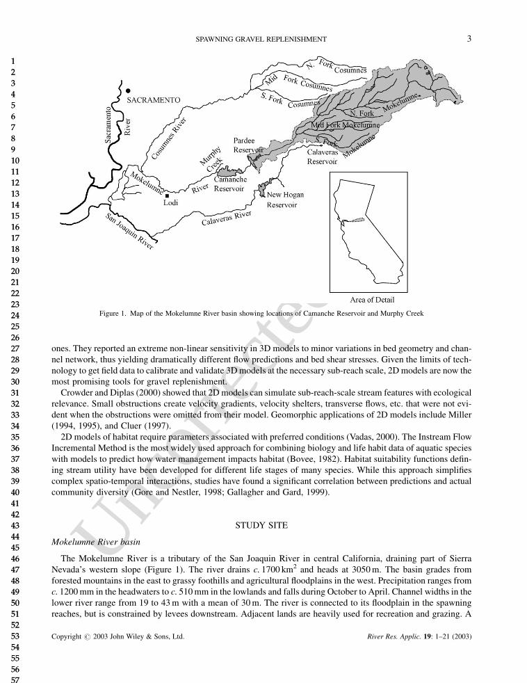
The Mokelumne River is a tributary of the San Joaquin River in central California, draining part of Sierra

Nevada’s western slope (Figure 1). The river drains c. 1700 km2 and heads at 3050 m. The basin grades from

forested mountains in the east to grassy foothills and agricultural floodplains in the west. Precipitation ranges from

c. 1200 mm in the headwaters to c. 510 mm in the lowlands and falls during October to April. Channel widths in the

lower river range from 19 to 43 m with a mean of 30 m. The river is connected to its floodplain in the spawning

reaches, but is constrained by levees downstream. Adjacent lands are heavily used for recreation and grazing. A

Figure 1. Map of the Mokelumne River basin showing locations of Camanche Reservoir and Murphy Creek

SPAWNING GRAVEL REPLENISHMENT 3


1

2

3

4

5

6

7

8

9

10

11

12

13

14

15

16

17

18

19

20

21

22

23

24

25

26

27

28

29

30

31

32

33

34

35

36

37

38

39

40

41

42

43

44

45

46

47

48

49

50

51

52

53

54

55

56

57

58

59

60

61

62

63

64

65

1

2

3

4

5

6

7

8

9

10

11

12

13

14

15

16

17

18

19

20

21

22

23

24

25

26

27

28

29

30

31

32

33

34

35

36

37

38

39

40

41

42

43

44

45

46

47

48

49

50

51

52

53

54

55

56

57

58

59

60

61

62

63

64

65

Uncor

recte

d Pr

oof

Uncor

recte

d Pr

oof

small tributary, Murphy Creek, enters the river c. 1 km downstream of the dam (Figure 1). Detailed hydrology,

geology, and ecology for the basin were presented in Wang and Pasternack (2000).

Flow regime

The Mokelumne River has 16 major water projects with four large reservoirs. The two most downstream reser-

voirs non-passable to anadromous fish are Pardee (completed in 1929) and Camanche (completed in 1963).

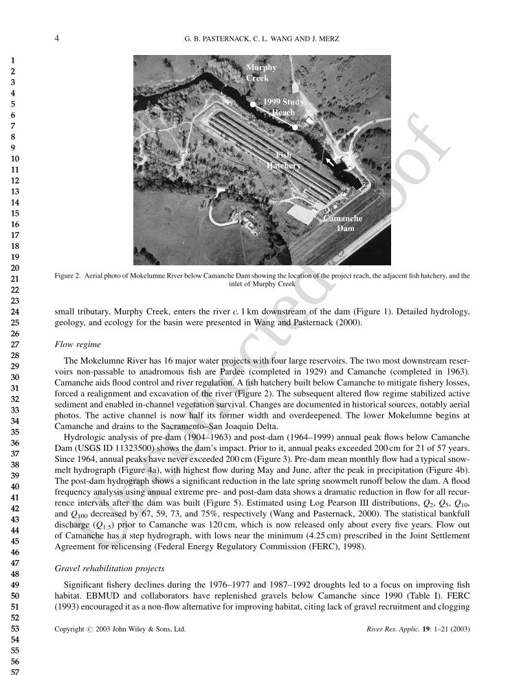
Camanche aids flood control and river regulation. A fish hatchery built below Camanche to mitigate fishery losses,

forced a realignment and excavation of the river (Figure 2). The subsequent altered flow regime stabilized active

sediment and enabled in-channel vegetation survival. Changes are documented in historical sources, notably aerial

photos. The active channel is now half its former width and overdeepened. The lower Mokelumne begins at

Camanche and drains to the Sacramento–San Joaquin Delta.

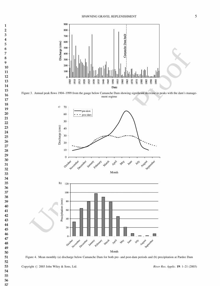
Hydrologic analysis of pre-dam (1904–1963) and post-dam (1964–1999) annual peak flows below Camanche

Dam (USGS ID 11323500) shows the dam’s impact. Prior to it, annual peaks exceeded 200 cm for 21 of 57 years.

Since 1964, annual peaks have never exceeded 200 cm (Figure 3). Pre-dam mean monthly flow had a typical snow-

melt hydrograph (Figure 4a), with highest flow during May and June, after the peak in precipitation (Figure 4b).

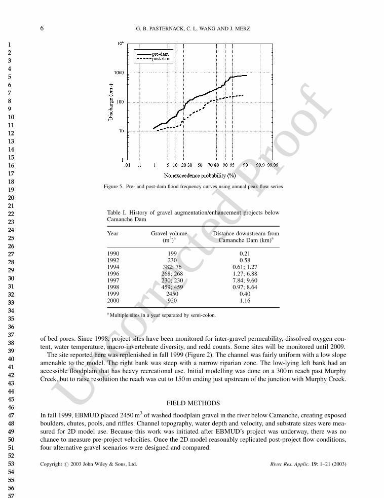
The post-dam hydrograph shows a significant reduction in the late spring snowmelt runoff below the dam. A flood

frequency analysis using annual extreme pre- and post-dam data shows a dramatic reduction in flow for all recur-

rence intervals after the dam was built (Figure 5). Estimated using Log Pearson III distributions, Q2, Q5, Q10,

and Q100 decreased by 67, 59, 73, and 75%, respectively (Wang and Pasternack, 2000). The statistical bankfull

discharge (Q1.5) prior to Camanche was 120 cm, which is now released only about every five years. Flow out

of Camanche has a step hydrograph, with lows near the minimum (4.25 cm) prescribed in the Joint Settlement

Agreement for relicensing (Federal Energy Regulatory Commission (FERC), 1998).

Gravel rehabilitation projects

Significant fishery declines during the 1976–1977 and 1987–1992 droughts led to a focus on improving fish

habitat. EBMUD and collaborators have replenished gravels below Camanche since 1990 (Table I). FERC

(1993) encouraged it as a non-flow alternative for improving habitat, citing lack of gravel recruitment and clogging

Figure 2. Aerial photo of Mokelumne River below Camanche Dam showing the location of the project reach, the adjacent fish hatchery, and theinlet of Murphy Creek



1

2

3

4

5

6

7

8

9

10

11

12

13

14

15

16

17

18

19

20

21

22

23

24

25

26

27

28

29

30

31

32

33

34

35

36

37

38

39

40

41

42

43

44

45

46

47

48

49

50

51

52

53

54

55

56

57

58

59

60

61

62

63

64

65

1

2

3

4

5

6

7

8

9

10

11

12

13

14

15

16

17

18

19

20

21

22

23

24

25

26

27

28

29

30

31

32

33

34

35

36

37

38

39

40

41

42

43

44

45

46

47

48

49

50

51

52

53

54

55

56

57

58

59

60

61

62

63

64

65

Uncor

recte

d Pr

oof

Uncor

recte

d Pr

oof

Figure 3. Annual peak flows 1904–1999 from the gauge below Camanche Dam showing significant decrease in peaks with the dam’s manage-ment regime

Figure 4. Mean monthly (a) discharge below Camanche Dam for both pre- and post-dam periods and (b) precipitation at Pardee Dam



1

2

3

4

5

6

7

8

9

10

11

12

13

14

15

16

17

18

19

20

21

22

23

24

25

26

27

28

29

30

31

32

33

34

35

36

37

38

39

40

41

42

43

44

45

46

47

48

49

50

51

52

53

54

55

56

57

58

59

60

61

62

63

64

65

1

2

3

4

5

6

7

8

9

10

11

12

13

14

15

16

17

18

19

20

21

22

23

24

25

26

27

28

29

30

31

32

33

34

35

36

37

38

39

40

41

42

43

44

45

46

47

48

49

50

51

52

53

54

55

56

57

58

59

60

61

62

63

64

65

Uncor

recte

d Pr

oof

Uncor

recte

d Pr

oof

of bed pores. Since 1998, project sites have been monitored for inter-gravel permeability, dissolved oxygen con-

tent, water temperature, macro-invertebrate diversity, and redd counts. Some sites will be monitored until 2009.

The site reported here was replenished in fall 1999 (Figure 2). The channel was fairly uniform with a low slope

amenable to the model. The right bank was steep with a narrow riparian zone. The low-lying left bank had an

accessible floodplain that has heavy recreational use. Initial modelling was done on a 300 m reach past Murphy

Creek, but to raise resolution the reach was cut to 150 m ending just upstream of the junction with Murphy Creek.

FIELD METHODS

In fall 1999, EBMUD placed 2450 m3 of washed floodplain gravel in the river below Camanche, creating exposed

boulders, chutes, pools, and riffles. Channel topography, water depth and velocity, and substrate sizes were mea-

sured for 2D model use. Because this work was initiated after EBMUD’s project was underway, there was no

chance to measure pre-project velocities. Once the 2D model reasonably replicated post-project flow conditions,

four alternative gravel scenarios were designed and compared.

Figure 5. Pre- and post-dam flood frequency curves using annual peak flow series

Table I. History of gravel augmentation/enhancement projects belowCamanche Dam

Year Gravel volume Distance downstream from(m3)a Camanche Dam (km)a

1990 199 0.211992 230 0.581994 382; 76 0.61; 1.271996 268; 268 1.27; 6.881997 230; 230 7.84; 9.601998 459; 459 0.97; 8.641999 2450 0.402000 920 1.16

a Multiple sites in a year separated by semi-colon.



1

2

3

4

5

6

7

8

9

10

11

12

13

14

15

16

17

18

19

20

21

22

23

24

25

26

27

28

29

30

31

32

33

34

35

36

37

38

39

40

41

42

43

44

45

46

47

48

49

50

51

52

53

54

55

56

57

58

59

60

61

62

63

64

65

1

2

3

4

5

6

7

8

9

10

11

12

13

14

15

16

17

18

19

20

21

22

23

24

25

26

27

28

29

30

31

32

33

34

35

36

37

38

39

40

41

42

43

44

45

46

47

48

49

50

51

52

53

54

55

56

57

58

59

60

61

62

63

64

65

Uncor

recte

d Pr

oof

Uncor

recte

d Pr

oof

Channel topography

Detailed topography was mapped with 1155 points. Surveying was performed by licensed professionals and was

done before and after gravel placement while flow was low. Surveying resolution was high (c. 1 point per 3.6 m2).

Rather than using a uniform distribution (time-consuming in the field) or many transects (do not capture true topo-

graphy), care was taken to accurately map bed features with a high density of points measured in the vicinity of

natural slope breaks and fewer points over flat surfaces. In addition to coordinates, wet/dry channel boundaries,

water surface elevation, and bed exposure were carefully documented.

Observation data

Depth and velocity were measured after the gravel was placed at a typical spawning-season low flow (9.3 cm)

and a higher flow (31 cm). The high flow was close to the post-dam Q1.5, which is the Qbf suitable for evaluating

gravel scour (California Department of Fish and Game (CDFG), 1991). Though the peak for 1999 was 68 cm, this

could not be modelled because it spread over the unmapped floodplain.

Post-project depth and velocity were measured at four cross-sections. Endpoints were marked with steel pins to

define location and alignment. Endpins were surveyed with a Trimble Pathfinder Pro XRS differential GPS whose

resolution was c. 0.3 m. GPS coordinates were overlaid in the model to locate the nearest node to each endpin

thereby defining comparable cross-sections. Cross-sections 4 ( just upstream of placed gravel) and 7 (over gravel

bars) were waded at 9.3 cm and sampled every 0.3 m with careful position control. Depths were measured with a

stadia rod. At cross-section 4, velocity was averaged over 1 min with a Unidata Starflow depth-averaging ultrasonic

Doppler velocity meter (�1 mm s�1). At cross-section 7, a Marsh-McBirney Flo-mate (�33 mm s�1) and a depth-

setting wading rod were used to estimate average velocity as the point velocity at 0.6 of depth. Cross-sections 1

(upstream boundary for coarse mesh runs) and 10 (below placed gravel) were observed at 31 cm with a cable-

mounted USGS Price AA current meter from a flat-bottomed boat locked onto a high-tension steel cable every

1.5 m with careful position control. Standard USGS procedure for calculating depth-averaged velocity from point

measurements was used. Positional accuracy and observation resolution were much finer than the scale of bed

features (c. 5–10 m) and similar to model node spacing.

Substrate size

Wolman pebble counts were conducted before and after replenishment (Kondolf and Li, 1992). Counts were

made along three randomly located 30 m longitudinal transects yielding 300 particles. The first particle encoun-

tered by the tip of the index finger with closed eyes was sampled. This was done for 100 particles per transect. Each

particle was placed into 0.5 phi size class over the range of 3–8 phi including lumped <3 and >8 size fractions

(Vyverberg et al., 1996). Cumulative percentages of each class were calculated.

MOKELUMNE MODEL

Model description

The Finite Element Surface Water Modelling System Two-Dimensional Flow in a Horizontal Plane model

(FESWMS-2DH v. 2) simulates steady or unsteady 2D surface-water flows, including sub- and super-critical con-

ditions (Froehlich, 1989). FESWMS solves the vertically integrated equations of motion and continuity with a

finite element scheme. It uses a robust wetting and drying routine that determines channel boundary location.

An element is ‘dry’ when depth is below a user-defined threshold (0.12 m here) at all of its nodes.

FESWMS was implemented in the Boss International Surface Water Modelling System v. 7.0 (SMS). SMS was

used for finite element mesh creation and interpolation of topography to mesh nodes with a TIN-based linear topo-

graphic interpolation scheme. Initially a coarse mesh including Murphy Creek was used, but then model area was

reduced to 5091 m2 with the project and adjacent pool downstream. Elements were c. 1 m2 with a nodal distance of

c. 0.5 m (i.e. node centred in each element). Pre- and post-project meshes were trimmed close to the known wetted

perimeter for each flow to allow for a favourable balance between resolution of relevant bed features and compu-

tation time as well as to reduce wetting and drying computations.



1

2

3

4

5

6

7

8

9

10

11

12

13

14

15

16

17

18

19

20

21

22

23

24

25

26

27

28

29

30

31

32

33

34

35

36

37

38

39

40

41

42

43

44

45

46

47

48

49

50

51

52

53

54

55

56

57

58

59

60

61

62

63

64

65

1

2

3

4

5

6

7

8

9

10

11

12

13

14

15

16

17

18

19

20

21

22

23

24

25

26

27

28

29

30

31

32

33

34

35

36

37

38

39

40

41

42

43

44

45

46

47

48

49

50

51

52

53

54

55

56

57

58

59

60

61

62

63

64

65

Uncor

recte

d Pr

oof

Uncor

recte

d Pr

oof

Model parameterization

Model parameters were determined using theory and measurement. Camanche outflow was the discharge at the

upstream boundary. Water surface elevation was field-surveyed at the downstream boundary (28.1 m for 9.3 cm,

28.6 m for 31 cm). A global constant roughness coefficient (Manning’s n) of 0.043 was estimated based on rough-

ness tables for a straight, coarse gravel channel with no vegetation (McCuen, 1989). A spatially explicit algorithm

for roughness based on substrate size variations was unwarranted in this study for two reasons. First, the reach had

a narrow range of gravel substrate sizes, especially after gravel placement. Second, the form drag of gravel bars

caused much more significant roughness. Tests of spatially explicit roughness yielded no significant effect, match-

ing Miller and Cluer (1998).

FEWSMS uses the Boussinesq eddy viscosity to resolve turbulence closure. Eddy viscosity coefficient values

that are too high suppress flow separation, whereas values too low cause model instability (Miller, 1994). Eddy

viscosity was calculated as v ¼ C u� Rh, where C¼ 0.6, u�¼ shear velocity, and Rh¼ hydraulic radius (Froehlich,

1989). Shear velocity was calculated from velocity observations using Einstein’s log-velocity equation for turbu-

lent flow over rough beds. Even though calculated eddy viscosities were mostly <0.05 m2 s�1, values

<0.065 m2 s�1 led to model instability, so 0.065 m2 s�1 was used for all pre- and post-project model runs.

Scenario construction

Four alternative scenarios were designed using the SMS Scatter Point Module to compare against the actual ad

hoc placement. Even though SMS was not intended for topographic design, it was possible to create topography

using its scatter point module. Bed features were first created with artificial points and then pasted over existing

topography. Transitions between the pre-existing bed and artificial features were smoothed with additional topo-

graphic points.

Given the numerous artificial degrees of freedom in designing alternative reach topography (c. 3025 000), an

objective search for the optimal solution to habitat goals and sediment entrainment constraints was not feasible.

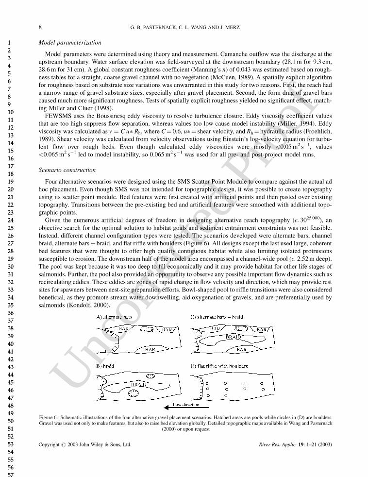
Instead, different channel configuration types were tested. The scenarios developed were alternate bars, channel

braid, alternate barsþ braid, and flat riffle with boulders (Figure 6). All designs except the last used large, coherent

bed features that were thought to offer high quality contiguous habitat while also limiting isolated protrusions

susceptible to erosion. The downstream half of the model area encompassed a channel-wide pool (c. 2.52 m deep).

The pool was kept because it was too deep to fill economically and it may provide habitat for other life stages of

salmonids. Further, the pool also provided an opportunity to observe any possible important flow dynamics such as

recirculating eddies. These eddies are zones of rapid change in flow velocity and direction, which may provide rest

sites for spawners between nest-site preparation efforts. Bowl-shaped pool to riffle transitions were also considered

beneficial, as they promote stream water downwelling, aid oxygenation of gravels, and are preferentially used by

salmonids (Kondolf, 2000).

Figure 6. Schematic illustrations of the four alternative gravel placement scenarios. Hatched areas are pools while circles in (D) are boulders.Gravel was used not only to make features, but also to raise bed elevation globally. Detailed topographic maps available in Wang and Pasternack

(2000) or upon request



1

2

3

4

5

6

7

8

9

10

11

12

13

14

15

16

17

18

19

20

21

22

23

24

25

26

27

28

29

30

31

32

33

34

35

36

37

38

39

40

41

42

43

44

45

46

47

48

49

50

51

52

53

54

55

56

57

58

59

60

61

62

63

64

65

1

2

3

4

5

6

7

8

9

10

11

12

13

14

15

16

17

18

19

20

21

22

23

24

25

26

27

28

29

30

31

32

33

34

35

36

37

38

39

40

41

42

43

44

45

46

47

48

49

50

51

52

53

54

55

56

57

58

59

60

61

62

63

64

65

Uncor

recte

d Pr

oof

Uncor

recte

d Pr

oof

Because the gravel needed for different scenarios varied by up to 30%, comparisons were made based on effi-

ciency—habitat area per cubic metre of gravel added. Gravel volumes were calculated by digital elevation model

(DEM) differencing in ArcInfo. Instream features were exposed at low flow by design. Gravel was used not only to

make features, but also to decrease water depths globally, as depth was universally greater than the optimal habitat

suitability value. Depth and velocity distribution statistics were taken from nodal data sets.

Model parameters were nearly the same as those used in pre- and post-project runs. The roughness coefficient

was 0.043 for all cases. Eddy viscosity was 0.065 m2 s�1 for all runs, except for the low flow alternate barsþ braid

run, for which it was 0.09 m2 s�1 due to model instability. Meshes had equal numbers of nodes and nearly equal

numbers of elements.

Scenario comparison

Scenarios were compared using habitat and sediment entrainment criteria. A global habitat suitability index

(GHSI) was calculated from velocity (VHSI) and depth (DHSI) suitability curves derived from 98 observed redds

at seven sites on the lower Mokelumne (CDFG, 1991). These curves were compared against independent data from

the Yuba and Sacramento rivers and found to be similar (CDFG, 1991). The GHSI is specifically for chinook sal-

mon spawning in the lower Mokelumne River under the assumption of perfect substrate quality, which holds when

new gravel is placed. DHSI and VHSI range from 0 to 1.13 m and 0 to 1.55 m s�1 with optimal conditions at 0.40 m

and 0.82 m s�1, respectively. These criteria were combined using GHSI¼DHSI(0.5)�VHSI(0.5). GHSI was classed

as poor (0–0.1), low (0.1–0.4), medium (0.4–0.7) and high (0.7–1.0) quality habitat (sensu Leclerc et al., 1995).

GHSI is calculated at each node and thus cannot assess spatially related habitats. Areas of each GHSI category in

each alternative design were calculated and compared.

To assess if placed gravels would wash away at the modelled flows, the ratio of actual to critical velocity was

used as a sediment mobility index (SMI). The depth-average critical velocity for movement of the median grain

size at a node was calculated using Einstein’s log-velocity equation for turbulent flows over rough beds combined

with Shield’s incipient motion criteria (Garde and Ranga Raju, 1985) assuming a dimensionless shear stress of

0.045:

�ucritical ¼ 5:75 log 12:2H

ks

� �� 0:045ð�s � �fÞd50

�f

� �0:5

ð1Þ

where H¼water depth, d50¼median bed material grain size, ks¼ boundary roughness, �s ¼ sediment specific

weight, �f¼fluid specific weight, and �f¼fluid density. For the Mokelumne’s highly homogeneous bed, d50

was taken as ks (Smart, 1999). This parameter should not be confused with the Z0 boundary roughness of a more

general form of Equation 1, though the two are linearly related (Smart, 1999). Because sediment is unlikely to

move under the low flow at which fish spawn (unless flow becomes supercritical), reported SMIs were calculated

under near-bankfull flow conditions. SMI >1 predicts entrainment. For SMI <1, entrainment potential was divided

into low (0–0.33), medium (0.33–0.67), and high (0.67–1.0) categories. Other causes of entrainment that are not

quantifiable in this model include fishermen walking on the gravel, gravel consolidation over time, local scour

around large woody debris (LWD), and salmon activity.

RESULTS

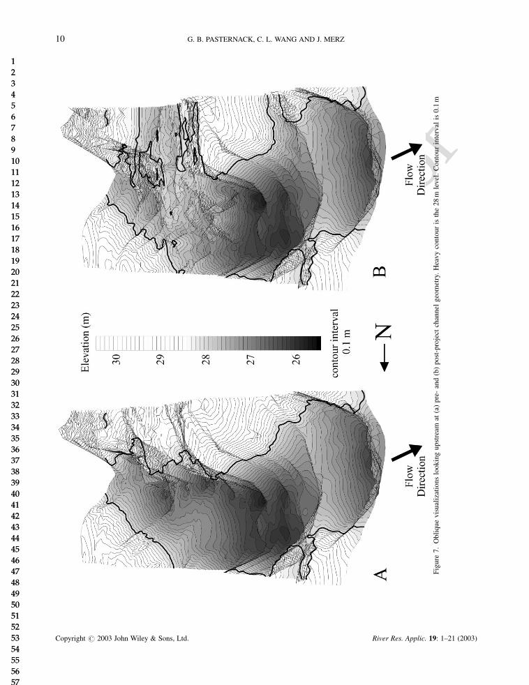
Gravel placement resulted in significant changes to the channel. Prior to the project, the channel was deep and

fairly uniform (Figure 7A) and had a bed composed of poorly sorted, compacted gravels of poor quality for salmon

spawning. Grain size frequency analysis showed a pre-project bed d50 of 41� 43 mm (1 standard deviation)

(Figure 8). A fraction (13%) of bed particles were <8 mm in diameter, potentially clogging large pores. After

the project the channel was shallow and diverse, with several longitudinal bars separated by fast-running chutes

(Figure 7B). The far right side of the channel had gravel scattered in small mounds to create exposed bars and

riffles under low flow. Exposed boulders were also used to create habitat features. Post-project d50 was

48� 21 mm yielding a homogeneous bed with large interstices (Figure 8). For both pre- and post-project



1

2

3

4

5

6

7

8

9

10

11

12

13

14

15

16

17

18

19

20

21

22

23

24

25

26

27

28

29

30

31

32

33

34

35

36

37

38

39

40

41

42

43

44

45

46

47

48

49

50

51

52

53

54

55

56

57

58

59

60

61

62

63

64

65

1

2

3

4

5

6

7

8

9

10

11

12

13

14

15

16

17

18

19

20

21

22

23

24

25

26

27

28

29

30

31

32

33

34

35

36

37

38

39

40

41

42

43

44

45

46

47

48

49

50

51

52

53

54

55

56

57

58

59

60

61

62

63

64

65

Uncor

recte

d Pr

oof

Uncor

recte

d Pr

oof

Fig

ure

7.

Ob

liq

ue

vis

ual

izat

ion

slo

ok

ing

up

stre

amat

(a)

pre

-an

d(b

)p

ost

-pro

ject

chan

nel

geo

met

ry.

Hea

vy

con

tou

ris

the

28

mle

vel

.C

on

tou

rin

terv

alis

0.1

m



1

2

3

4

5

6

7

8

9

10

11

12

13

14

15

16

17

18

19

20

21

22

23

24

25

26

27

28

29

30

31

32

33

34

35

36

37

38

39

40

41

42

43

44

45

46

47

48

49

50

51

52

53

54

55

56

57

58

59

60

61

62

63

64

65

1

2

3

4

5

6

7

8

9

10

11

12

13

14

15

16

17

18

19

20

21

22

23

24

25

26

27

28

29

30

31

32

33

34

35

36

37

38

39

40

41

42

43

44

45

46

47

48

49

50

51

52

53

54

55

56

57

58

59

60

61

62

63

64

65

Uncor

recte

d Pr

oof

Uncor

recte

d Pr

oof

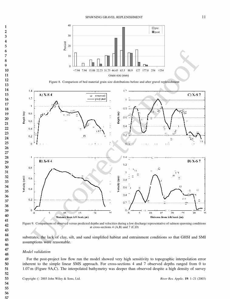
substrates, the lack of clay, silt, and sand simplified habitat and entrainment conditions so that GHSI and SMI

assumptions were reasonable.

Model validation

For the post-project low flow run the model showed very high sensitivity to topographic interpolation error

inherent to the simple linear SMS approach. For cross-sections 4 and 7 observed depths ranged from 0 to

1.07 m (Figure 9A,C). The interpolated bathymetry was deeper than observed despite a high density of survey

Figure 8. Comparison of bed material grain size distributions before and after gravel replenishment

Figure 9. Comparisons of observed versus predicted depths and velocities during a low discharge representative of salmon spawning conditionsat cross-sections 4 (A,B) and 7 (C,D)



1

2

3

4

5

6

7

8

9

10

11

12

13

14

15

16

17

18

19

20

21

22

23

24

25

26

27

28

29

30

31

32

33

34

35

36

37

38

39

40

41

42

43

44

45

46

47

48

49

50

51

52

53

54

55

56

57

58

59

60

61

62

63

64

65

1

2

3

4

5

6

7

8

9

10

11

12

13

14

15

16

17

18

19

20

21

22

23

24

25

26

27

28

29

30

31

32

33

34

35

36

37

38

39

40

41

42

43

44

45

46

47

48

49

50

51

52

53

54

55

56

57

58

59

60

61

62

63

64

65

Uncor

recte

d Pr

oof

Uncor

recte

d Pr

oof

points. Cross-section 7 had three bars, three chutes, and a small side channel on the right bank yielding a significant

challenge for SMS.

Differences in observed versus predicted velocity primarily stemmed from the topographic interpolation error.

Cross-section 4 had an observed peak velocity of 0.78 m s�1. Predicted velocities nearly equalled the five observed

values (Figure 9B). Data were lost for the right side of the channel due to battery failure. At cross-section 7,

observed velocities were underpredicted in chutes and overpredicted over gravel bars (Figure 9D).

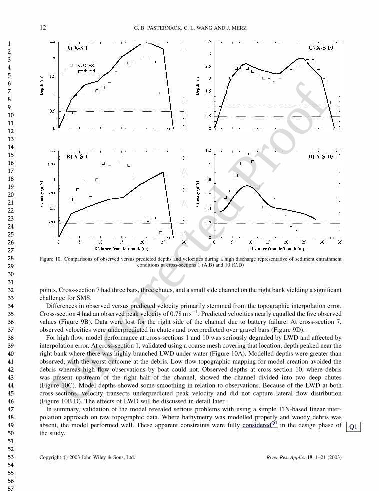
For high flow, model performance at cross-sections 1 and 10 was seriously degraded by LWD and affected by

interpolation error. At cross-section 1, validated using a coarse mesh covering that location, depth peaked near the

right bank where there was highly branched LWD under water (Figure 10A). Modelled depths were greater than

observed, with the worst outcome at the debris. Low flow topographic mapping for model creation avoided the

debris whereas high flow observations by boat could not. Observed depths at cross-section 10, where debris

was present upstream of the right half of the channel, showed the channel divided into two deep chutes

(Figure 10C). Model depths showed some smoothing in relation to observations. Because of the LWD at both

cross-sections, velocity transects underpredicted peak velocity and did not capture lateral flow distribution

(Figure 10B,D). The effects of LWD will be discussed in detail later.

In summary, validation of the model revealed serious problems with using a simple TIN-based linear inter-

polation approach on raw topographic data. Where bathymetry was modelled properly and woody debris was

absent, the model performed well. These apparent constraints were fully consideredQ1 in the design phase of

the study.

Figure 10. Comparisons of observed versus predicted depths and velocities during a high discharge representative of sediment entrainmentconditions at cross-sections 1 (A,B) and 10 (C,D)

Q1



1

2

3

4

5

6

7

8

9

10

11

12

13

14

15

16

17

18

19

20

21

22

23

24

25

26

27

28

29

30

31

32

33

34

35

36

37

38

39

40

41

42

43

44

45

46

47

48

49

50

51

52

53

54

55

56

57

58

59

60

61

62

63

64

65

1

2

3

4

5

6

7

8

9

10

11

12

13

14

15

16

17

18

19

20

21

22

23

24

25

26

27

28

29

30

31

32

33

34

35

36

37

38

39

40

41

42

43

44

45

46

47

48

49

50

51

52

53

54

55

56

57

58

59

60

61

62

63

64

65

Uncor

recte

d Pr

oof

Uncor

recte

d Pr

oof

Scenario results

Even though model validation showed that SMS provided poor topographic interpolation in complex terrain so

that depth and velocity were underestimated, this deficiency has no impact on comparison of different scenarios

with prescribed topography. To compare between real channel configurations and prescribed alternatives required

the assumption of accurately interpolated topography. For the pre-project case, the channel was uniform enough

that the model reasonably represented topography. For the post-project case, the model was accurate away from

bars and chutes but not over such features. Thus, post-project results presented below underestimate details of flow

and habitat conditions.

Overall, bed, flow, habitat, and sediment entrainment conditions for the six different bed topographies varied

significantly. Model output is illustrated in a series of four maps per scenario: depth, velocity, GHSI at low flow,

and SMI at high flow. For the sake of brevity, depth and SMI plots are excluded, though relevant aspects of these

plots are summarized below. All plots and raw data sets from this study are available in Wang and Pasternack

(2000) or by request.

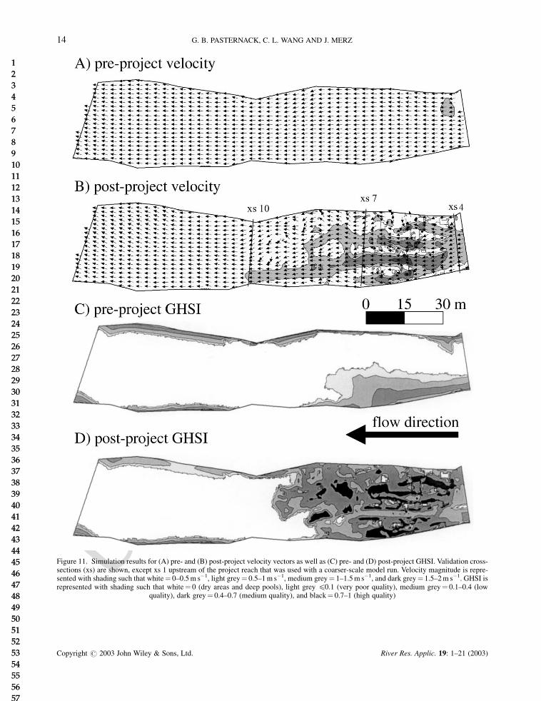
The pre-project baseline consisted of a uniform channel with low velocities, minimal spawning habitat, and no

sediment entrainment (Figure 11A,C). Depths spanned 0–1.82 m, while velocities ranged from 0 to 0.60 m s�1.

Velocity vectors were generally parallel and showed little deviation from the longitudinal axis (Figure 11A). Depth

controlled GHSI values given low and nearly constant velocities (Figure 11C). The channel was too deep to yield

habitat for 74% of the area, leaving a usable fringe along the banks. No high quality habitat was predicted. Mon-

itoring from 1990 to 1998 showed no salmon spawning activity (Setka, 2000), confirming the model prediction.

High depths and low velocities uniformly yielded very low SMI values.

EBMUD’s gravel replenishment yielded significantly different and highly complex fluvio-geomorphic condi-

tions (Figure 11B,D). Depth decreased to 0.15–1 m, with the bed exposed over boulders and bar tops. Shallow

depths produced faster flows that funnelled between exposed features (Figure 11B). Chute velocities ranged from

1.64 to 2.04 m s�1. A large eddy behind a boulder in both observed and modelled conditions indicated accurate

representation of flow pattern, if not flow magnitude. GHSI values were dramatically enhanced due to decreased

depth, though the best habitat was highly patchy (Figure 11D). Except for exposed bar tops, the entire project area

became usable habitat. Velocities in the fastest chute were too high and produced low quality habitat. Other chutes

and some riffle areas produced high quality habitat. Shallower depths and faster velocities increased SMI values,

but no entrainment was predicted. Critical velocities were nearly exceeded in cells adjacent to exposed bars.

Because the model underpredicted chute velocities, the site was field inspected and these small areas were found

to indeed be eroding while other areas were stable as predicted.

In the alternate bars scenario, two small bars were placed on the right bank and one big bar on the left bank

(Figure 6A). Opposing bars were connected by riffles; a pool separated the two riffles. Because the reach was short,

bars were not intended to mimic natural riffle–pool spacing, but rather to provide simple, coherent bed structures

with low risk of erosion during spawning season. The alternate bars decreased channel width, causing flow mean-

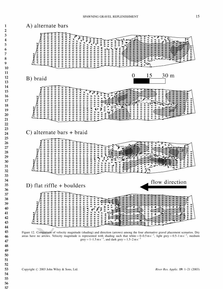
dering as well as recirculating eddies downstream of all bars. Bar tops were dry at low flow. Velocities ranged from

0 to 1.28 m s�1 (Figure 12A). Despite lacking habitat on exposed bars, the same amount of high quality habitat was

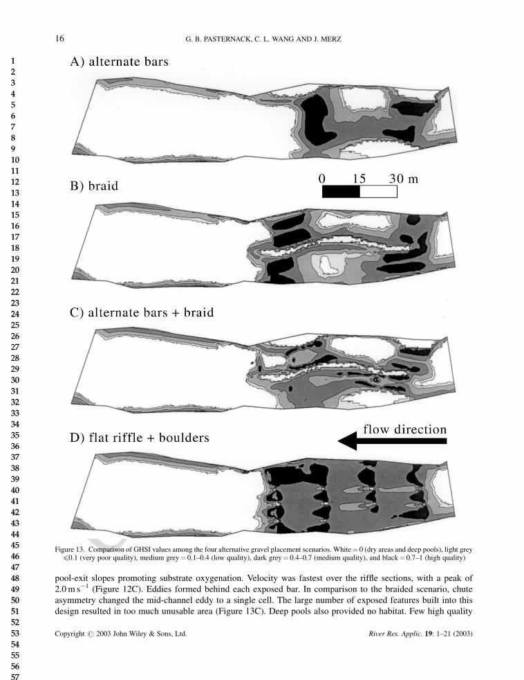
predicted as for the actual post-project case (Figure 13A). Habitat was concentrated in three large patches on shal-

low riffles. SMIs showed no erosion. The highest SMI occurred at the head of the first alternate bar.

In the braided scenario, an exposed 76� 5 m sinuous braid was placed mid-channel to divide flow into two

spawning chutes. A riffle–pool–riffle sequence was made in each chute yielding three pool–riffle transitions

promoting water downwelling and substrate oxygenation (Figure 6B). Velocities ranged from 0 to 1.13 m s�1

(Figure 12B). Recirculating eddies formed in the shear zone along the braid’s upper half. A large two-cell eddy

formed over the braid’s lower section and a single-cell eddy formed downstream along the right bank. High quality

habitat occurred along riffle sections (Figure 13B). Depth and velocity conditions conflicted with each other limit-

ing potential habitat. SMIs were higher over riffles but still too low for entrainment.

The alternate barsþ braid scenario had two meandering chutes with riffle–pool–riffle sequences (Figure 6C).

The left sequence was highly constricted between the braid and the bar because the left bar was much bigger than

the two bars forming the right bank. The size of the bar limited the size and depth of the pool in the left chute. This

formed a narrow chute over a riffle that led to a shallow pool and then to another riffle. Once again there were three



1

2

3

4

5

6

7

8

9

10

11

12

13

14

15

16

17

18

19

20

21

22

23

24

25

26

27

28

29

30

31

32

33

34

35

36

37

38

39

40

41

42

43

44

45

46

47

48

49

50

51

52

53

54

55

56

57

58

59

60

61

62

63

64

65

1

2

3

4

5

6

7

8

9

10

11

12

13

14

15

16

17

18

19

20

21

22

23

24

25

26

27

28

29

30

31

32

33

34

35

36

37

38

39

40

41

42

43

44

45

46

47

48

49

50

51

52

53

54

55

56

57

58

59

60

61

62

63

64

65

Uncor

recte

d Pr

oof

Uncor

recte

d Pr

oof

Figure 11. Simulation results for (A) pre- and (B) post-project velocity vectors as well as (C) pre- and (D) post-project GHSI. Validation cross-sections (xs) are shown, except xs 1 upstream of the project reach that was used with a coarser-scale model run. Velocity magnitude is repre-sented with shading such that white¼ 0–0.5 m s�1, light grey¼ 0.5–1 m s�1, medium grey¼ 1–1.5 m s�1, and dark grey¼ 1.5–2 m s�1. GHSI isrepresented with shading such that white¼ 0 (dry areas and deep pools), light grey 40.1 (very poor quality), medium grey¼ 0.1–0.4 (low

quality), dark grey¼ 0.4–0.7 (medium quality), and black¼ 0.7–1 (high quality)



1

2

3

4

5

6

7

8

9

10

11

12

13

14

15

16

17

18

19

20

21

22

23

24

25

26

27

28

29

30

31

32

33

34

35

36

37

38

39

40

41

42

43

44

45

46

47

48

49

50

51

52

53

54

55

56

57

58

59

60

61

62

63

64

65

1

2

3

4

5

6

7

8

9

10

11

12

13

14

15

16

17

18

19

20

21

22

23

24

25

26

27

28

29

30

31

32

33

34

35

36

37

38

39

40

41

42

43

44

45

46

47

48

49

50

51

52

53

54

55

56

57

58

59

60

61

62

63

64

65

Uncor

recte

d Pr

oof

Uncor

recte

d Pr

oof

Figure 12. Comparison of velocity magnitude (shading) and direction (arrows) among the four alternative gravel placement scenarios. Dryareas have no arrows. Velocity magnitude is represented with shading such that white¼ 0–0.5 m s�1, light grey¼ 0.5–1 m s�1, medium

grey¼ 1–1.5 m s�1, and dark grey¼ 1.5–2 m s�1



1

2

3

4

5

6

7

8

9

10

11

12

13

14

15

16

17

18

19

20

21

22

23

24

25

26

27

28

29

30

31

32

33

34

35

36

37

38

39

40

41

42

43

44

45

46

47

48

49

50

51

52

53

54

55

56

57

58

59

60

61

62

63

64

65

1

2

3

4

5

6

7

8

9

10

11

12

13

14

15

16

17

18

19

20

21

22

23

24

25

26

27

28

29

30

31

32

33

34

35

36

37

38

39

40

41

42

43

44

45

46

47

48

49

50

51

52

53

54

55

56

57

58

59

60

61

62

63

64

65

Uncor

recte

d Pr

oof

Uncor

recte

d Pr

oof

pool-exit slopes promoting substrate oxygenation. Velocity was fastest over the riffle sections, with a peak of

2.0 m s�1 (Figure 12C). Eddies formed behind each exposed bar. In comparison to the braided scenario, chute

asymmetry changed the mid-channel eddy to a single cell. The large number of exposed features built into this

design resulted in too much unusable area (Figure 13C). Deep pools also provided no habitat. Few high quality

Figure 13. Comparison of GHSI values among the four alternative gravel placement scenarios. White¼ 0 (dry areas and deep pools), light grey40.1 (very poor quality), medium grey¼ 0.1–0.4 (low quality), dark grey¼ 0.4–0.7 (medium quality), and black¼ 0.7–1 (high quality)



1

2

3

4

5

6

7

8

9

10

11

12

13

14

15

16

17

18

19

20

21

22

23

24

25

26

27

28

29

30

31

32

33

34

35

36

37

38

39

40

41

42

43

44

45

46

47

48

49

50

51

52

53

54

55

56

57

58

59

60

61

62

63

64

65

1

2

3

4

5

6

7

8

9

10

11

12

13

14

15

16

17

18

19

20

21

22

23

24

25

26

27

28

29

30

31

32

33

34

35

36

37

38

39

40

41

42

43

44

45

46

47

48

49

50

51

52

53

54

55

56

57

58

59

60

61

62

63

64

65

Uncor

recte

d Pr

oof

Uncor

recte

d Pr

oof

habitat areas existed, as optimal depth coincided with excessive velocity, while optimal velocity occurred in exces-

sive depth. Relatively high SMI values were concentrated at the head of the first alternate bar.

For the flat riffleþ boulders scenario, gravel was set uniformly over the site. Ten boulders were spaced evenly

over the left 67% of the channel to constrict flow, create high velocities, and obtain small recirculating eddies pro-

viding resting locations for juveniles and adults (Figure 6D). Boulders were c. 3 m in diameter and exposed at low

flow. The upstream end of the riffle had a broad pool-exit slope for water downwelling. The fastest velocities

occurred in the constrictions between boulders, typically 0.5–1.22 m s�1 (Figure 12D). Velocities were lowest

behind boulders (c. 0.01–0.5 m s�1). Due to the uniformity of gravel and lack of exposed areas, this scenario

yielded the most habitat area, though the most gravel was used too (Figure 13D). Boulder symmetry produced

regularly distributed high quality habitat patches in the optimal velocity chutes between boulders. Highest SMIs

occurred in grid cells just upstream of each boulder.

DISCUSSION

Several studies explain the effect of sparse topographic data on 2D modelling (Anderson and Bates, 1994; French

and Clifford, 2000; Marks and Bates, 2000), but few have addressed the significance of DEM-generation limita-

tions within 2D modelling packages. This project had dense data surveyed by professionals yielding a high quality

baseline at the scale of habitat-relevant features. This assisted the design of alternatives and enabled a test of SMS

and FESWMS in comparing designs on the basis of habitat and sediment entrainment patterns. Unfortunately,

SMS v. 7.0 proved unable to generate a digital elevation model that accurately reflected complex natural topogra-

phy, even with a node spacing of 0.5 m. Lacking that, FESWMS could not match observed conditions. SMS does

not have enough tools for accurate terrain modelling. While its topographic interpolation scheme is identical to

other DEM software, what is needed is better management of large and layered topographic datasets as well as

options to apply accepted civil engineering methods that manually adjust the terrain model to yield an accurate

representation as can be done with many CAD programs, such as AutoDesk’s AutoCAD. DEMs made using engi-

neering software may be imported into SMS and used with a 2D model to yield more computationally stable and

accurate simulations. Thus, in addition to collecting dense topographic datasets, one must work hard at DEM gen-

eration to obtain an accurate representation of the bed for 2D modelling.

Even with an accurate terrain model, a serious problem was encountered in representing flow conditions near

LWD. While woody material was not widespread, two large pieces altered the flow pattern of the model validation

cross-sections. Resulting errors affected habitat quality estimates and location as well as potential for sediment

entrainment. As large woody debris can provide significant instream habitat (Abbe and Montgomery, 1996; Merz,

2001) and is part of channel rehabilitation, this poses a limitation on the use of a 2D model where wood is present.

Changing local flow parameters to better mimic woody debris can help a model match observed conditions, but this

is not possible in a design mode predicting future velocities under alternatives. Further, habitat provided by woody

debris is not accounted for in habitat suitability indices, so the use of model results to predict habitat conditions

would be tenuous.

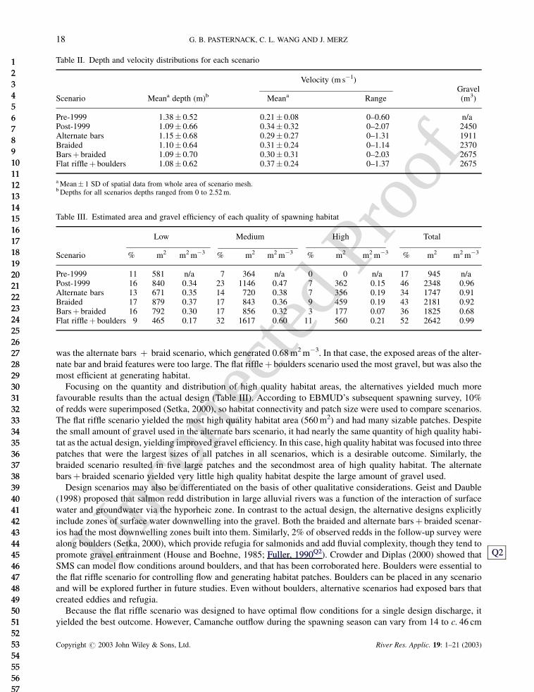
Gravel replenishment yielded a dramatic change in flow conditions and thus in quantity and quality of habitat.

Mean depth decreased from 1.38 m to 1.09 m, while predicted mean velocity increased from 0.21 to 0.34 m s�1

(Table II). More importantly, the range of predicted velocities increased from 0–0.6 to 0–2.07 m s�1. Because

the model underestimated actual velocity (Figures 9 and 10), and higher velocity would have yielded higher GHSI

values, habitat quality was underestimated. Even so, the site went from having no high quality habitat to having at

least 362 m2 of it. Total usable habitat changed from 945 to over 2350 m2, with the largest increase occurring for

medium quality habitat. The efficiency of the gravel project was 0.96 m2 m�3. Whereas no spawning occurred in

the reach in prior years, after gravel placement redds were observed on-site within two months. The follow year

there were 29 redds on-site (out of 987 for the whole lower river). These changes show gravel replenishment sig-

nificantly improves quantity and quality of habitat, even without an objective design process.

Comparing the predicted quantity of habitat under different scenarios showed that many produced similar out-

comes (Table III). Even though designed bed features had large exposed areas that provided no habitat, their struc-

tures yielded more efficient habitat generation in between so overall gravel efficiency was 0.91–0.99 m2 m�3,

which was comparable to the ad hoc project. The only scenario that resulted in a very poor utilization of gravel



1

2

3

4

5

6

7

8

9

10

11

12

13

14

15

16

17

18

19

20

21

22

23

24

25

26

27

28

29

30

31

32

33

34

35

36

37

38

39

40

41

42

43

44

45

46

47

48

49

50

51

52

53

54

55

56

57

58

59

60

61

62

63

64

65

1

2

3

4

5

6

7

8

9

10

11

12

13

14

15

16

17

18

19

20

21

22

23

24

25

26

27

28

29

30

31

32

33

34

35

36

37

38

39

40

41

42

43

44

45

46

47

48

49

50

51

52

53

54

55

56

57

58

59

60

61

62

63

64

65

Uncor

recte

d Pr

oof

Uncor

recte

d Pr

oof

was the alternate bars þ braid scenario, which generated 0.68 m2 m�3. In that case, the exposed areas of the alter-

nate bar and braid features were too large. The flat riffleþ boulders scenario used the most gravel, but was also the

most efficient at generating habitat.

Focusing on the quantity and distribution of high quality habitat areas, the alternatives yielded much more

favourable results than the actual design (Table III). According to EBMUD’s subsequent spawning survey, 10%

of redds were superimposed (Setka, 2000), so habitat connectivity and patch size were used to compare scenarios.

The flat riffle scenario yielded the most high quality habitat area (560 m2) and had many sizable patches. Despite

the small amount of gravel used in the alternate bars scenario, it had nearly the same quantity of high quality habi-

tat as the actual design, yielding improved gravel efficiency. In this case, high quality habitat was focused into three

patches that were the largest sizes of all patches in all scenarios, which is a desirable outcome. Similarly, the

braided scenario resulted in five large patches and the secondmost area of high quality habitat. The alternate

barsþ braided scenario yielded very little high quality habitat despite the large amount of gravel used.

Design scenarios may also be differentiated on the basis of other qualitative considerations. Geist and Dauble

(1998) proposed that salmon redd distribution in large alluvial rivers was a function of the interaction of surface

water and groundwater via the hyporheic zone. In contrast to the actual design, the alternative designs explicitly

include zones of surface water downwelling into the gravel. Both the braided and alternate barsþ braided scenar-

ios had the most downwelling zones built into them. Similarly, 2% of observed redds in the follow-up survey were

along boulders (Setka, 2000), which provide refugia for salmonids and add fluvial complexity, though they tend to

promote gravel entrainment (House and Boehne, 1985; Fuller, 1990Q2). Crowder and Diplas (2000) showed that

SMS can model flow conditions around boulders, and that has been corroborated here. Boulders were essential to

the flat riffle scenario for controlling flow and generating habitat patches. Boulders can be placed in any scenario

and will be explored further in future studies. Even without boulders, alternative scenarios had exposed bars that

created eddies and refugia.

Because the flat riffle scenario was designed to have optimal flow conditions for a single design discharge, it

yielded the best outcome. However, Camanche outflow during the spawning season can vary from 14 to c. 46 cm

Table III. Estimated area and gravel efficiency of each quality of spawning habitat

Low Medium High Total

Scenario % m2 m2 m�3 % m2 m2 m�3 % m2 m2 m�3 % m2 m2 m�3

Pre-1999 11 581 n/a 7 364 n/a 0 0 n/a 17 945 n/aPost-1999 16 840 0.34 23 1146 0.47 7 362 0.15 46 2348 0.96Alternate bars 13 671 0.35 14 720 0.38 7 356 0.19 34 1747 0.91Braided 17 879 0.37 17 843 0.36 9 459 0.19 43 2181 0.92Barsþ braided 16 792 0.30 17 856 0.32 3 177 0.07 36 1825 0.68Flat riffleþ boulders 9 465 0.17 32 1617 0.60 11 560 0.21 52 2642 0.99

Table II. Depth and velocity distributions for each scenario

Velocity (m s�1)Gravel

Scenario Meana depth (m)b Meana Range (m3)

Pre-1999 1.38� 0.52 0.21� 0.08 0–0.60 n/aPost-1999 1.09� 0.66 0.34� 0.32 0–2.07 2450Alternate bars 1.15� 0.68 0.29� 0.27 0–1.31 1911Braided 1.10� 0.64 0.31� 0.24 0–1.14 2370Barsþ braided 1.09� 0.70 0.30� 0.31 0–2.03 2675Flat riffleþ boulders 1.08� 0.62 0.37� 0.24 0–1.37 2675

a Mean� 1 SD of spatial data from whole area of scenario mesh.b Depths for all scenarios depths ranged from 0 to 2.52 m.

Q2



1

2

3

4

5

6

7

8

9

10

11

12

13

14

15

16

17

18

19

20

21

22

23

24

25

26

27

28

29

30

31

32

33

34

35

36

37

38

39

40

41

42

43

44

45

46

47

48

49

50

51

52

53

54

55

56

57

58

59

60

61

62

63

64

65

1

2

3

4

5

6

7

8

9

10

11

12

13

14

15

16

17

18

19

20

21

22

23

24

25

26

27

28

29

30

31

32

33

34

35

36

37

38

39

40

41

42

43

44

45

46

47

48

49

50

51

52

53

54

55

56

57

58

59

60

61

62

63

64

65

Uncor

recte

d Pr

oof

Uncor

recte

d Pr

oof

between years. Under such a range, matching a single design flow in any given year is unlikely unless dam opera-

tions specify it. Deviation from the design discharge would yield little to no usable habitat. In contrast, the other

design approaches would provide a suitable area of habitat under a range of flows because of their topographic

complexity.

No sediment entrainment for the median grain size was predicted for any scenarios at near-bankfull flow

(31 cm). The scenarios with sites that were approaching an entrainment condition were the actual design and

the flat riffle with boulders. In both cases potential entrainment was located at the heads of boulders and bars.

Ideally, the model would be used to simulate higher flows, but above-bankfull conditions induce flooding of the

adjacent forested floodplain, which could not be modelled at a reasonable cost. In 1986 the California Department

of Fish and Game performed a simple sediment study for the Mokelumne River using HEC-6 (CDFG, 1991). At a

cross-section just upstream of the site, they predicted that at c. 30 cm, grain sizes of 44.6 mm would be entrained.

Even at a flow of c. 142 cm, HEC-6 predicted that only sizes smaller than 12.5 mm would be transported. As the

added gravel had a median size of 48 mm, constructed features should be well protected against flow-induced

gravel loses. Based on observation, a greater concern may be erosion by supercritical flow at extremely low flow

depths.

In this study it was found that an off-the-shelf 2D modelling package could be used to design and compare alter-

native scenarios for gravel rehabilitation of salmon spawning sites on the basis of multiple quantitative and qua-

litative habitat and sediment mobility criteria. When an accurate DEM is generated using a high-density

topographic survey and professional design engineering software, then a hydrodynamic model can accurately

simulate spatial patterns in velocity, depth, sediment entrainment, and spawning habitat in streams. By comparing

these variables for six different channel configurations it was possible to distinguish design features that generated

and enhanced physical habitat from those that were counterproductive. The strongest conclusion reached is that ad

hoc gravel replenishment yields highly patchy habitat conditions that are less gravel-efficient and more likely to

erode. Even with large areas of exposed gravel, alternative designs matched or exceeded the actual design. The use

of exposed gravel at the design flow is warranted when higher than normal discharges are planned for. In this case,

flow may be lower than the design discharge, so it would have been better to keep bars submerged. With that addi-

tional area, alternatives would probably greatly exceed the actual design in habitat area and gravel efficiency.

Among alternatives, the braided scenario would have been selected for construction because of its large amount

of total and high quality habitat, its gravel efficiency, its generation of multiple oxygenation zones and one- or two-

cell recirculating eddies, and its lack of sediment entrainment. This choice is probably unique to this site, and many

other possible alternatives were not considered in the design phase.

ACKNOWLEDGEMENTS

We gratefully acknowledge James Smith, Dr Jeff Mount, Dr David Galut, Dr Michel Leclerc, Joe Wheaton,

Brett Valle, Jose Constantine, and anonymous reviewers for input to the research and manuscript. Russ Taylor

and other EBMUD staff helped with data collection while Ellen Mantalica at UC Davis provided logistical support.

REFERENCES

Abbe TB, Montgomery DR. 1996. Large woody debris jams, channel hydrodynamics and habitat formation in large rivers. Regulated Rivers:

Research & Management 12: 201–221.

Allan JD, Flecker AS. 1993. Biodiversity conservation in running waters. BioScience 43: 32–43.

Anderson MG, Bates PD. 1994. Evaluating data constraints on two-dimensional finite element models of floodplain flow. Catena 22: 1–15.

Bovee KD. 1982. Perspectives on two-dimensional river habitat models: the PHABSIM experience. Proceedings 2nd International Symposium

on Habitat Hydraulics. B150–B162.Q3

Brandt SA. 2000. Classification of geomorphological effects downstream of dams. Catena 40: 375–401.

California Department of Fish and Game. 1991. Lower Mokelumne River Fisheries Management Plan. The Resources Agency: Sacramento,

CA.

California Department of Water Resources. 1995. Sacramento River Gravel Restoration Phase II Study: A Plan for Continued Spawning Gravel

Replenishment Between Keswick Dam and Clear Creek. Technical Information Record TIR ND-95-1, Northern District: Red Bluff, CA.

Q3



1

2

3

4

5

6

7

8

9

10

11

12

13

14

15

16

17

18

19

20

21

22

23

24

25

26

27

28

29

30

31

32

33

34

35

36

37

38

39

40

41

42

43

44

45

46

47

48

49

50

51

52

53

54

55

56

57

58

59

60

61

62

63

64

65

1

2

3

4

5

6

7

8

9

10

11

12

13

14

15

16

17

18

19

20

21

22

23

24

25

26

27

28

29

30

31

32

33

34

35

36

37

38

39

40

41

42

43

44

45

46

47

48

49

50

51

52

53

54

55

56

57

58

59

60

61

62

63

64

65

Uncor

recte

d Pr

oof

Uncor

recte

d Pr

oof

Castleberry DT, Czech JJ, Erman DC, Hankin D, Healey M, Kondolf GM, Mangel M, Mohr M, Moyle PB, Nielsen J, Speed TP, Williams JG.

1996. Uncertainty and instream flow standards. Fisheries 21: 20–21.Q4Chapman WM. 1943. The spawning of chinook salmon in the main Columbia River. Copeia 1943: 168–170

Cluer BL. 1997. Eddy bar responses to the sediment dynamics of pool-riffle environments. PhD Dissertation, Colorado State University, Fort

Collins.

Crowder DW, Diplas P. 2000. Using two-dimensional hydrodynamic models at scales of ecological importance. Journal of Hydrology 230:

172–191.

Douglas AJ, Taylor JG. 1998. Riverine based eco-tourism: Trinity River non-market benefits analysis. International Journal of Sustainable

Development and World Ecology 5: 136–148.

Federal Energy Regulatory Commission. 1993. Final Environmental Impact Statement, Proposed Modifications to the Lower Mokelumne River

Project, California, FERC Project No. 2916–004. Federal Energy Regulatory Commission: Washington, DC.Q4Fetherston SC. 1994. Channel Adjustments to Camanche Dam on the Mokelumne River, California. University of California: Berkeley.

French JR, Clifford NJ. 2000. Hydrodynamic modeling as a basis for explaining estuarine environmental dynamics: some computational and

methodological issues. Hydrological Processes 14: 2089–2108.

Froehlich DC. 1989. Finite Element Surface-Water Modeling System: Two-dimensional Flow in a Orizontal Plane User’s Manual. US Depart-

ment of Transportation, Publication #FHWA-RD-88-177.

Gallagher SP, Gard MF. 1999. Relationship between Chinook salmon (Oncorhynchus tshawytscha) redd densities and PHABSIM-predicted

habitat in the Merced and Lower American rivers, California. Canadian Journal of Fisheries and Aquatic Sciences 56: 570–577.

Garde RJ, Ranga Raju KG. 1985. Mechanics of Sediment Transportation and Alluvial Stream Problems. Wiley Eastern Limited: New Dehli.

Geist DR, Dauble DD. 1998. Redd site selection and spawning habitat use by fall Chinook salmon: the importance of geomorphic features in

large rivers. Environmental Management 22: 655–669.

Ghanem A, Steffler P, Hicks F. 1996. Two-dimensional hydraulic simulation of physical habitat conditions in flowing streams. Regulated Rivers:

Research & Management 12: 185–200.

Gilvear DJ, Waters TM, Milner AM. 1995. Image analysis of aerial photography to quantify changes in channel morphology and instream

habitat following placer mining in interior Alaska. Freshwater Biology 34: 389–398.

Gore JA, Nestler JM. 1998. Instream flow studies in perspective. Regulated Rivers: Research & Management 2: 93–101.Q4Habersack H, Nachtnebel P. 1995. Short-term effects of local river restoration on morphology, flow field, substrate and biota. Regulated

Rivers: Research & Management 10: 291–301.

Harvey BC, Lisle TE. 1998. Effects of suction dredging on streams: a review and an evaluation strategy. Fisheries 23: 8–17.

House R, Boehne P. 1985. Evaluation of instream enhancement structures for salmonid spawning and rearing in a coastal Oregon stream. North

American Journal of Fisheries Management 5: 283–295.

Kondolf GM. 1997. Hungry water: effects of dams and gravel mining on river channels. Environmental Management 21: 533–551.

Kondolf GM. 2000. Assessing salmonid spawning gravel quality. Transaction of the American Fisheries Society 129: 262–281.

Kondolf GM, Li S. 1992. The pebble count technique for quantifying surface bed material size in instream flow studies. Rivers 3: 80–87.

Kondolf GM, Matthews WVG. 1993. Management of Coarse Sediment in Regulated Rivers of California, Report No. 80. University of

California Water Resources Center: Riverside.

Kondolf GM, Vick JC, Ramirez TM. 1996. Salmon Spawning Habitat Rehabilitation in the Merced, Tuolumne, and Stanislaus Rivers, Cali-

fornia: An Evaluation of Project Planning and Performance, Report No. 90. University of California Water Resources Center: Berkeley, CA.

Lane SN, Bradbrook KF, Richards KS, Biron PA, Roy GA. 1999. The application of computational fluid dynamics to natural river channels:

three-dimensional versus two-dimensional approaches. Geomorphology 29: 1–20.

Leclerc M, Boudreault A, Bechara JA, Corfa G. 1995. Two-dimensional hydrodynamic modeling: a neglected tool in the instream flow incre-

mental methodology. Transactions of the American Fisheries Society 124: 645–662.

Marks K, Bates P. 2000. Integration of high-resolution topographic data with floodplain flow models. Hydrological Processes 14: 2109–2122.

Marks SD, Rutt GP. 1997. Fluvial sediment inputs to upland gravel bed rivers draining forested catchments: potential ecological impacts.

Hydrology and Earth System Sciences 1: 499–508.

McCuen RH. 1989. Hydrologic Analysis and Design. Prentice Hall: Englewood Cliffs.Q4McElhiney MA. 1992. Soil Survey of San Joaquin County, California. United States Soil Conservation Service.

Merz JE. 2001. Association of fall-run chinook salmon redds with woody debris in the lower Mokelumne River, California. Caliornia Fish and

Game 87: 51–60.

Miller AJ. 1994. Debris-fan constrictions and flood hydraulics in river canyons: some implications from two-dimensional flow modelling. Earth

Surface Processes and Landforms 19: 681–697.

Miller AJ. 1995. Valley morphology and boundary conditions influencing spatial patterns of flood flow. In Natural and Anthropogenic Influences

in Fluvial Geomorphology, Costa JE, Miller AJ, Potter KW, Wilcock PR (eds). American Geophysical Union: Washington, DC; 57–81.

Miller AJ, Cluer BL. 1998. Modeling considerations for simulation of flow in bedrock channels. In Rivers Over Rock: Fluvial Processes in

Bedrock Channels, Wohl EE, Tinkler KJ (eds). American Geophysical Union: Washington, DC; 61–104.

Moyle PB, Randall PJ. 1998. Evaluating the biotic integrity of watersheds in the Sierra Nevada, California. Conservation Biology 12: 1318–

1326.

Moyle PB, Marchetti MP, Baldrige J, Taylor TL. 1998. Fish health and diversity: justifying flows for a California stream. Fisheries 23: 6–15.

Nagasaka A, Nakamura F. 1999. The influences of land-use changes on hydrology and riparian environment in a northern Japanese landscape.

Landscape Ecology 14: 543–556.

Q4

Q4

Q4

Q4



1

2

3

4

5

6

7

8

9

10

11

12

13

14

15

16

17

18

19

20

21

22

23

24

25

26

27

28

29

30

31

32

33

34

35

36

37

38

39

40

41

42

43

44

45

46

47

48

49

50

51

52

53

54

55

56

57

58

59

60

61

62

63

64

65

1

2

3

4

5

6

7

8

9

10

11

12

13

14

15

16

17

18

19

20

21

22

23

24

25

26

27

28

29

30

31

32

33

34

35

36

37

38

39

40

41

42

43

44

45

46

47

48

49

50

51

52

53

54

55

56

57

58

59

60

61

62

63

64

65

Uncor

recte

d Pr

oof

Uncor

recte

d Pr

oof

National Marine Fisheries Service. 2001. Annual Commercial Landing Statistics. NMFS Fisheries Statistics and Economic Division:

Washington, DC.

National Research Council. 1992. Restoration of Aquatic Ecosystems: Science, Technology, and Public Policy. NRC Committee on Restoration

of Aquatic Ecosystems: Washington, DC.Q4Nawa RK, Frissell CA. 1993. Measuring scour and fill of gravel streambeds with scour chains and sliding bead monitors. North American

Journal of Fisheries Management 13: 634–639.

Nehlsen W, Williams JE, Lichatowich JA. 1991. Pacific salmon at the crossroads: stocks at risk from California, Oregon, Idaho, and

Washington. Fisheries 16: 4–21.

Petts GE. 1996. Water allocation to predict river ecosystems. Regulated Rivers: Research and Management 12: 353–365.Q4Piper AM, Galey HS, Thomas HE, Robinson TW. 1939. Geology and Ground-Water Hydrology of the Mokelumne Area, California. Water-

supply Paper 780. United States Geological Survey: Washington.

Platts WS, Megahan W. 1975. Time Trends in Channel Sediment Size Composition in Salmon and Steelhead Spawning Areas: South Fork

Salmon River, Idaho. USDA Forest Service General Technical Report. Internountal Forest and Range Experiment Station: Ogden, Utah.

Poff NL, Allan JD, Bain MB, Karr JR, Prestegaard KL, Richter BD, Sparks RE, Stromberg JC. 1997. The natural flow regime. BioScience 47:

769–784.

Sandecki M. 1989. Aggregate mining in river systems. California Geology 42: 88–94.

Setka JD. 2000. Fall-run Chinook Salmon and Steelhead Trout Spawning Survey, September 1999 Through January 2000 Mokelumne River,

California. East Bay Municipal Utility District: Lodi, CA.

Smart GM. 1999. Turbulent velocity profiles and boundary shear in gravel bed rivers. Journal of Hydraulic Engineering 125: 106–116.

Soulsby C, Youngson AF, Moir HJ, Malcolm IA. 2000. Fine sediment influence on salmonid spawning habitat in a lowland agricultural stream: a

preliminary assessment. The Science of the Total Environment 265: 295–307.Q4Stalnaker CB, Lamb BL, Henriksen J, Bovee K, Bartholow J. 1995. The Instream Flow Incremental Methodology: A Primer for IFIM.

Biological Report 29. US Department of the Interior, National Biological Service.Q4Stearns HT, Robinson TW, Taylor GH. 1930. Geology and Water Resources of the Mokelumne Area, California. Water-supply Paper 619.

United States Geological Survey: Washington, DC.

Vadas RL. 2000. Instream-flow needs for anadromous salmonids and lamprey on the Pacific Coast, with special reference to the Pacific South-

west. Environmental Monitoring and Assessment 64: 331–358.

Vyverberg K, Snider B, Titus RG. 1996. Lower American River Chinook Salmon Spawning Habitat Evaluation. California Department of Fish

and Game: Sacramento.

Yoshiyama RM, Fisher FW, Moyle PB. 1998. Historical abundance and decline of chinook salmon in the Central Valley region of California.

North American Journal of Fisheries Management 18: 487–521.

Wang CL, Pasternack GB. 2000. Application of a 2-D Hydraulic Model to Reach-scale Spawning Gravel Replenishment. University of

California.

Q4

Q4

Q4

Q4



1

2

3

4

5

6

7

8

9

10

11

12

13

14

15

16

17

18

19

20

21

22

23

24

25

26

27

28

29

30

31

32

33

34

35

36

37

38

39

40

41

42

43

44

45

46

47

48

49

50

51

52

53

54

55

56

57

58

59

60

61

62

63

64

65

1

2

3

4

5

6

7

8

9

10

11

12

13

14

15

16

17

18

19

20

21

22

23

24

25

26

27

28

29

30

31

32

33

34

35

36

37

38

39

40

41

42

43

44

45

46

47

48

49

50

51

52

53

54

55

56

57

58

59

60

61

62

63

64

65

Uncor

recte

d Pr

oof

Uncor

recte

d Pr

oof

Author Query Form (RRA/748)

Special Instructions: Author please write responses to queries directly on Galley proofs

and then fax back. Alternatively please list responses in an e-mail.

Q1: Author: OK?

Q2: Author: Not in ref. list.

Q3: Author: Publisher? Place published?

Q4: Author: Not cited.

1

2

3

4

5

6

7

8

9

10

11

12

13

14

15

16

17

18

19

20

21

22

23

24

25

26

27

28

29

30

31

32

33

34

35

36

37

38

39

40

41

42

43

44

45

46

47

48

49

50

51

52

53

54

55

56

57

58

59

60

61

62

63

64

65

1

2

3

4

5

6

7

8

9

10

11

12

13

14

15

16

17

18

19

20

21

22

23

24

25

26

27

28

29

30

31

32

33

34

35

36

37

38

39

40

41

42

43

44

45

46

47

48

49

50

51

52

53

54

55

56

57

58

59

60

61

62

63

64

65

Documents

RIVER RESEARCH AND APPLICATIONS APPLICATION OF A 2D