Embed Size (px)
Citation preview
Rochester Institute of Technology Rochester Institute of Technology
RIT Scholar Works RIT Scholar Works
Theses
8-2016
Learning for Cross-layer Resource Allocation in the Framework of Learning for Cross-layer Resource Allocation in the Framework of
Cognitive Wireless Networks Cognitive Wireless Networks
Wenbo Wang [email protected]
Follow this and additional works at: https://scholarworks.rit.edu/theses
Recommended Citation Recommended Citation Wang, Wenbo, "Learning for Cross-layer Resource Allocation in the Framework of Cognitive Wireless Networks" (2016). Thesis. Rochester Institute of Technology. Accessed from
This Dissertation is brought to you for free and open access by RIT Scholar Works. It has been accepted for inclusion in Theses by an authorized administrator of RIT Scholar Works. For more information, please contact [email protected].
LEARNING FOR CROSS-LAYER RESOURCE
ALLOCATION IN THE FRAMEWORK OF
COGNITIVE WIRELESS NETWORKS
by
Wenbo Wang
DISSERTATION
Presented to the Faculty of the Golisano College of Computer and
Information Sciences
Rochester Institute of Technology
in Partial Fulfillment
of the Requirements
for the Degree of
DOCTOR OF PHILOSOPHY
Rochester Institute of Technology
August 2016
Learning for Cross-Layer Resource Allocation in the Framework of
Cognitive Wireless Networks
by
Wenbo Wang
Committee Approval: We, the undersigned committee members, certify that we have advised and/or supervised the
candidate on the work described in this dissertation. We further certify that we have reviewed the
dissertation manuscript and approve it in partial fulfillment of the requirements of the degree of
Doctor of Philosophy in Computing and Information Sciences.
______________________________________________________________________________
Dr. Andres Kwasinski Date
Dissertation Advisor
______________________________________________________________________________
Dr. Zhu Han Date
Dissertation Committee Member
______________________________________________________________________________
Dr. Pengcheng Shi Date
Dissertation Committee Member
______________________________________________________________________________
Dr. Kaiqi Xiong Date
Dissertation Committee Member
______________________________________________________________________________
Dr. Shanchieh Jay Yang Date
Dissertation Committee Member
______________________________________________________________________________
Dr. Drew N. Maywar Date
Dissertation Defense Chair
Certified by:
______________________________________________________________________________
Dr. Pengcheng Shi Date
Director, Computing and Information Sciences
Acknowledgments
I would like to thank my adviser, Dr. Andres Kwasinski, for all his advice,
support and patience since I entered the Ph.D. program of Golisano College
of Computer and Information Sciences in RIT. I would like to thank Prof.
Shanchieh Jay Yang, Prof. Zhu Han, Dr. Kaiqi Xiong and Prof. Pengcheng
Shi for being on my dissertation committee. I also would like to thank Prof.
Shanchieh Jay Yang and Prof. Pengcheng Shi for their invaluable advice and
encouragement when I was at the lowest point of my life.
Finally, I would like to thank my parents for their unconditional love and
support. Without their support, I would not have been able to complete my
Ph.D. study.
iii
Abstract
LEARNING FOR CROSS-LAYER RESOURCE ALLOCATION IN
THE FRAMEWORK OF COGNITIVE WIRELESS NETWORKS
Author: Wenbo Wang
Supervisor: Andres Kwasinski, Ph.D.
Degree: Doctor of Philosophy
Golisano College of Computing and Information Sciences, 2016
The framework of cognitive wireless networks is expected to endow wireless
devices with a cognition-intelligence ability with which they can efficiently
learn and respond to the dynamic wireless environment. In this dissertation,
we focus on the problem of developing cognitive network control mechanisms
without knowing in advance an accurate network model. We study a series of
cross-layer resource allocation problems in cognitive wireless networks. Based
on model-free learning, optimization and game theory, we propose a framework
of self-organized, adaptive strategy learning for wireless devices to (implicitly)
build the understanding of the network dynamics through trial-and-error.
The work of this dissertation is divided into three parts. In the first
part, we investigate a distributed, single-agent decision-making problem for
real-time video streaming over a time-varying wireless channel between a sin-
gle pair of transmitter and receiver. By modeling the joint source-channel
resource allocation process for video streaming as a constrained Markov de-
cision process, we propose a reinforcement learning scheme to search for the
optimal transmission policy without the need to know in advance the details
of network dynamics.
iv
In the second part of this work, we extend our study from the single-agent
to a multi-agent decision-making scenario, and study the energy-efficient power
allocation problems in a two-tier, underlay heterogeneous network and in a
self-sustainable green network. For the heterogeneous network, we propose
a stochastic learning algorithm based on repeated games to allow individual
macro- or femto-users to find a Stackelberg equilibrium without flooding the
network with local action information. For the self-sustainable green network,
we propose a combinatorial auction mechanism that allows mobile stations to
adaptively choose the optimal base station and sub-carrier group for transmis-
sion only from local payoff and transmission strategy information.
In the third part of this work, we study a cross-layer routing problem in
an interweaved Cognitive Radio Network (CRN), where an accurate network
model is not available and the secondary users that are distributed within the
CRN only have access to local action/utility information. In order to develop
a spectrum-aware routing mechanism that is robust against potential insider
attackers, we model the uncoordinated interaction between CRN nodes in the
dynamic wireless environment as a stochastic game. Through decomposition
of the stochastic routing game, we propose two stochastic learning algorithm
based on a group of repeated stage games for the secondary users to learn the
best-response strategies without the need of information flooding.
v
Table of Contents
Acknowledgments iii
Abstract iv
List of Tables ix
List of Figures x
Chapter 1. Introduction and Background 1
1.1 Cognitive Radio Networks . . . . . . . . . . . . . . . . . . . . 1
1.2 Strategy Learning for Cross-layer Network Resource Allocation 5
1.2.1 Joint source-channel coding control . . . . . . . . . . . . 6
1.2.2 Joint bandwidth and power allocation . . . . . . . . . . 7
1.2.3 Robust spectrum-aware relay selection . . . . . . . . . . 8
Chapter 2. Learning for Scalable Video Transmission with HARQover Dynamic Wireless Channels 10
2.1 Mathematical Description of Scalable Video Transmission Process 12
2.1.1 Rate-distortion model with scalable source coding . . . 12
2.1.2 Impact of channel coding on distortion model . . . . . . 15
2.1.3 Sub-frame level data transmission with HARQ . . . . . 16
2.2 Adaptive Learning for Rate Adaption . . . . . . . . . . . . . . 20
2.2.1 Transmission control as a Markov decision process . . . 20
2.2.2 Model-free learning for optimal video streaming policy . 24
2.3 Simulation Results . . . . . . . . . . . . . . . . . . . . . . . . 26
2.4 Chapter Summary . . . . . . . . . . . . . . . . . . . . . . . . . 29
vi
Chapter 3. Learning for Self-organized Power Allocation in Het-erogeneous Network 31
3.1 Network Model and QoS Metric . . . . . . . . . . . . . . . . . 34
3.2 Power Allocation Based on Continuous Stackelberg Game . . . 37
3.2.1 Femtocell power allocation with continuous strategies . . 38
3.2.2 Approximate solution to the price of MBS . . . . . . . . 45
3.3 Learning for Power Allocation in Discrete Stackelberg Game . 48
3.4 Numerical Simulation Results . . . . . . . . . . . . . . . . . . 53
3.4.1 Continuous game equilibrium analysis . . . . . . . . . . 54
3.4.2 Discrete game equilibrium analysis . . . . . . . . . . . . 56
3.5 Chapter Summary . . . . . . . . . . . . . . . . . . . . . . . . . 60
Chapter 4. Learning for Joint Channel-Power Allocation in Self-Sustainable Wireless Networks 62
4.1 System Model . . . . . . . . . . . . . . . . . . . . . . . . . . . 64
4.1.1 Energy generation and consumption profile . . . . . . . 65
4.1.2 Joint subcarrier-power allocation for mobile stations . . 66
4.2 Hierarchical formulation of resource allocation . . . . . . . . . 69
4.2.1 Subcarrier scheduling as combinatorial auction . . . . . 69
4.3 Iterative Learning for Subcarrier Allocation . . . . . . . . . . . 72
4.3.1 Iterative auction mechanism for subcarrier allocation . . 72
4.3.2 Power price adjustment for subcarrier demand control . 75
4.4 Simulation Results . . . . . . . . . . . . . . . . . . . . . . . . 78
4.5 Chapter Summary . . . . . . . . . . . . . . . . . . . . . . . . . 82
Chapter 5. Learning for Robust Routing Based on StochasticGame in Cognitive Radio Networks 83
5.1 Challenges in Designing a Robust Routing Mechanism for CRNs 85
5.1.1 Routing in CRNs . . . . . . . . . . . . . . . . . . . . . . 85
5.1.2 Security issues for routing in CRNs . . . . . . . . . . . . 87
5.2 Network Model and Link Metric . . . . . . . . . . . . . . . . . 88
5.2.1 Dynamic spectrum access model . . . . . . . . . . . . . 88
5.2.2 Impact of node behavior on link quality . . . . . . . . . 90
5.2.3 Link quality metric . . . . . . . . . . . . . . . . . . . . 95
vii
5.2.4 Impact of malicious SUs . . . . . . . . . . . . . . . . . . 96
5.3 Strategy Learning for Robust Routing Based on Stochastic Game 97
5.3.1 Relay selection as a stochastic game . . . . . . . . . . . 97
5.3.2 Stochastic strategy learning based on truthful informa-tion exchange . . . . . . . . . . . . . . . . . . . . . . . . 106
5.3.3 Truth-telling enforcement through multi-arm bandit . . 115
5.4 Simulation Results . . . . . . . . . . . . . . . . . . . . . . . . 118
5.5 Chapter Summary . . . . . . . . . . . . . . . . . . . . . . . . . 124
Chapter 6. Summary and Future Work 125
6.1 Summary . . . . . . . . . . . . . . . . . . . . . . . . . . . . . . 125
6.2 Future Work . . . . . . . . . . . . . . . . . . . . . . . . . . . . 128
Bibliography 131
viii
List of Tables
2.1 Transition probabilities of the Markov model for layered videotransmission . . . . . . . . . . . . . . . . . . . . . . . . . . . . 21
2.2 Main parameters used in the video streaming simulation. . . . 27
2.3 Retransmission frequencies for the learning processes in Figure2.4. . . . . . . . . . . . . . . . . . . . . . . . . . . . . . . . . . 27
2.4 Performance comparison between different transmission mech-anisms. . . . . . . . . . . . . . . . . . . . . . . . . . . . . . . . 29
3.1 Main Parameters Used in the Femtocell Network Simulation . 54
3.2 Main Parameters Used in the Self-Learning Algorithm . . . . . 57
4.1 Iterative subcarrier auction mechanism . . . . . . . . . . . . . 76
4.2 Bisection Based Power Price Updating . . . . . . . . . . . . . 77
4.3 SWA Configuration Parameters for the Simulation . . . . . . . 80
ix
List of Figures
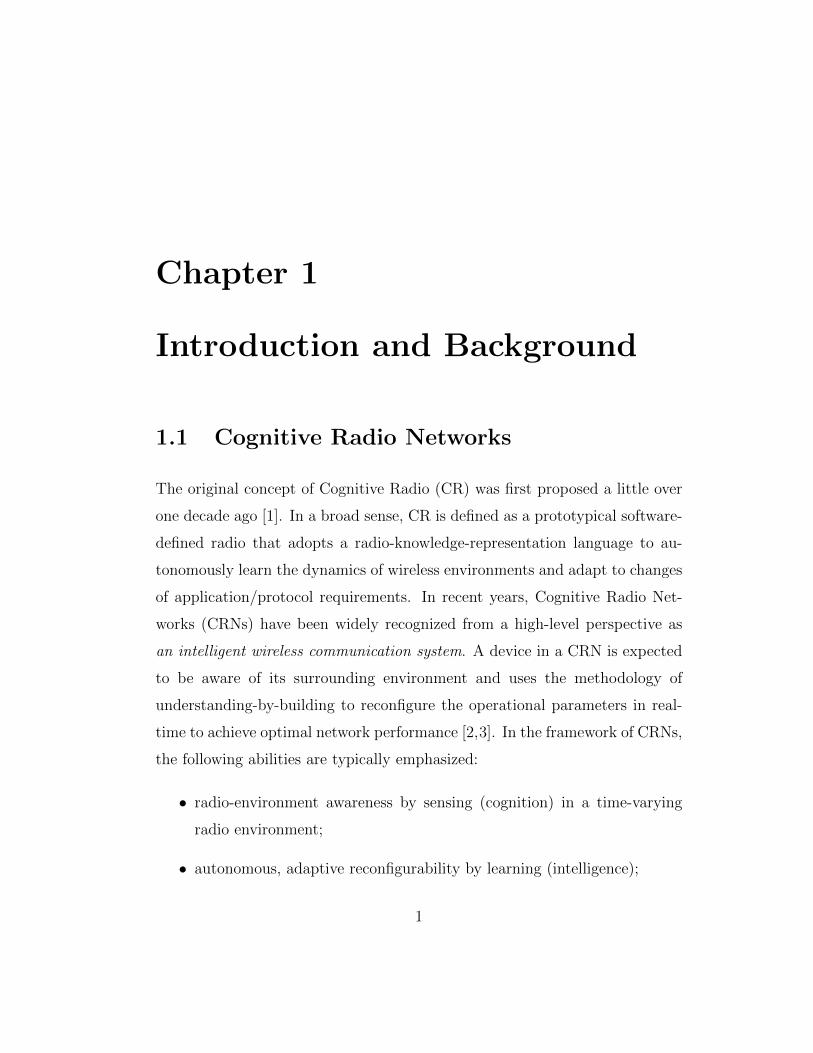
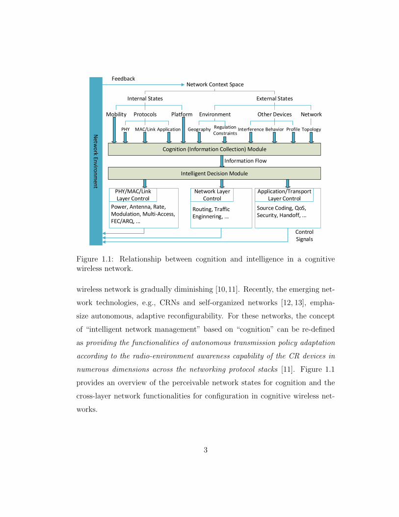
1.1 Relationship between cognition and intelligence in a cognitivewireless network. . . . . . . . . . . . . . . . . . . . . . . . . . 3
2.1 Dependency DAG of one GoP with both temporal and qualityscalability. . . . . . . . . . . . . . . . . . . . . . . . . . . . . . 13
2.2 The state transition for video layer n of GoP i . . . . . . . . . 19
2.3 Layered video transmission Markov chain. . . . . . . . . . . . 21
2.4 Transmission performance and policy evolution with the pro-posed adaptive policy learning mechanism. (a) Frame PSNRv.s. frame number. (b) Source-coding rate v.s. frame number. 28
3.1 Influence of the unit interference price on the NE of the contin-uous follower-game. (a) Average power efficiency at the NE vs.the unit price λ; (b) total revenue collected by the MBS at theNE vs. the unit price λ. . . . . . . . . . . . . . . . . . . . . . 55
3.2 MBS revenue and FU power efficiency at the SEs. (a) MBSrevenue vs. the number of FAPs; (b) FU power efficiency vs.the number of FAPs. . . . . . . . . . . . . . . . . . . . . . . . 56
3.3 Expected equilibrium SINR at the MU vs. the number of FAPs. 57
3.4 Influence of the unit interference price on the NE of the discretefollower-game. (a) Expected average power efficiency at the NEvs. the unit price λ; (b) total revenue collected by the MBS atthe NE vs. the unit price λ. . . . . . . . . . . . . . . . . . . . 58
3.5 Expected MBS revenue and FU power efficiency at the SEs inthe discrete strategy space. (a) MBS revenue vs. the numberof FAPs; (b) FU power efficiency vs. the number of FAPs. . . 59
3.6 Expected transmit power vs. the number of iterations. . . . . 59
3.7 Power selection probability vs. the number of iterations by FU 1. 60
x
4.1 An example of a microgrid with five BSs, in which the powersource is installed as a combination of different green powergenerators. . . . . . . . . . . . . . . . . . . . . . . . . . . . . . 63
4.2 The follower subgame (i.e., the subcarrier auction game) per-formance evolution during one time slot. (a) Total effectivethroughput v.s. auction rounds; (b) average power consump-tion v.s. auction rounds. . . . . . . . . . . . . . . . . . . . . . 78
4.3 Performance evolution with power pricing. (a) Power consump-tion/generation v.s. time; (b) total throughput v.s. time. . . . 81
4.4 Performance comparison. (a) Expected throughput withoutpower pricing; (b) percentage of operational time. . . . . . . . 82
5.1 Radio activities in a two-channel CRN with coordinated peri-odic sensing in the secondary network. . . . . . . . . . . . . . 89
5.2 SU links in a CRN with two clusters. . . . . . . . . . . . . . . 92
5.3 Attacker-free sensor grid network over a single PU channel. . . 119
5.4 Strategy evolution: relay selection probability vs. iterationnumber. . . . . . . . . . . . . . . . . . . . . . . . . . . . . . . 119
5.5 An attacker-free CRN over 2 PU channels. . . . . . . . . . . . 120
5.6 Strategy evolution: channel-relay selection probability vs. iter-ation number. . . . . . . . . . . . . . . . . . . . . . . . . . . . 120
5.7 Average path delay vs. number of flows for different algorithms. 121
5.8 (a) Frequency of connections to malicious nodes vs. scale forutility. (b) Average path delay vs. scale of exaggerated utilityby malicious nodes. . . . . . . . . . . . . . . . . . . . . . . . . 123
xi
Chapter 1
Introduction and Background
1.1 Cognitive Radio Networks
The original concept of Cognitive Radio (CR) was first proposed a little over
one decade ago [1]. In a broad sense, CR is defined as a prototypical software-
defined radio that adopts a radio-knowledge-representation language to au-
tonomously learn the dynamics of wireless environments and adapt to changes
of application/protocol requirements. In recent years, Cognitive Radio Net-
works (CRNs) have been widely recognized from a high-level perspective as
an intelligent wireless communication system. A device in a CRN is expected
to be aware of its surrounding environment and uses the methodology of
understanding-by-building to reconfigure the operational parameters in real-
time to achieve optimal network performance [2,3]. In the framework of CRNs,
the following abilities are typically emphasized:
• radio-environment awareness by sensing (cognition) in a time-varying
radio environment;
• autonomous, adaptive reconfigurability by learning (intelligence);
1
• cost-efficient and scalable network configuration.
Many recent studies on CR technologies focus on radio-environment aware-
ness in order to enhance spectrum efficiency. This leads to the concept of
Dynamic Spectrum Access (DSA) networks [4], which are featured by a novel
PHY-MAC architecture (namely, primary users and secondary users) for op-
portunistic spectrum access based on the detection of spectrum holes [5]. It
is worth noting that by emphasizing the network architecture of spectrum
sharing between the licensed/primary networks and the unlicensed/secondary
networks [4], “DSA networks” is frequently considered a terminology that is
interchangeable with “CR networks” [3]. The rationale behind such a consid-
eration is that a secondary network relies on spectrum cognition modules to
make proper decisions for seamless spectrum access without interfering the pri-
mary transmissions. For this category of works in the literature, “learning” is
a set of techniques for feature classification of primary signal identification [6].
For an overview of the relevant techniques, the readers may refer to recent
survey works in [7–9].
In order to achieve autonomous and cost-effective network configuration,
the functionality of self-organized, adaptive reconfigurability also become fun-
damental for CRNs, since this functionality shapes the network control and
transmission strategy acquisition mechanisms. By emphasizing on such an
objective, the network management mechanism is required to dynamically
characterize the situation of the decision-making entities in the network and
accordingly infer the proper transmission strategies. As the network man-
agement mechanisms in conventional wireless networks are acquiring more
and more levels of such a cognition-intelligence ability, the border between a
pure CRN, namely, a CRN in the sense of DSA networks, and a conventional
2
Network Context Space
Internal States External States
Mobility Protocols Platform Environment Other Devices Network
PHY MAC/Link Application Geography InterferenceRegulation
ConstraintsBehavior Profile Topology
Cognition (Information Collection) Module
Intelligent Decision Module
PHY/MAC/Link
Layer Control
Network Layer
Control
Ne
two
rk E
nviro
nm
en
t
Information Flow
Feedback
Control
Signals
Power, Antenna, Rate,
Modulation, Multi-Access,
FEC/ARQ, ...
Routing, Traffic
Enginnering, ...
Application/Transport
Layer Control
Source Coding, QoS,
Security, Handoff, ...
Figure 1.1: Relationship between cognition and intelligence in a cognitivewireless network.
wireless network is gradually diminishing [10,11]. Recently, the emerging net-
work technologies, e.g., CRNs and self-organized networks [12, 13], empha-
size autonomous, adaptive reconfigurability. For these networks, the concept
of “intelligent network management” based on “cognition” can be re-defined
as providing the functionalities of autonomous transmission policy adaptation
according to the radio-environment awareness capability of the CR devices in
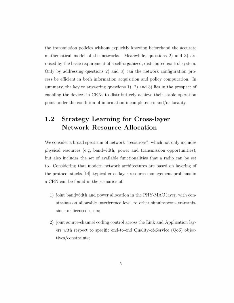
numerous dimensions across the networking protocol stacks [11]. Figure 1.1
provides an overview of the perceivable network states for cognition and the
cross-layer network functionalities for configuration in cognitive wireless net-
works.
3
Designing an efficient and robust cross-layer resource allocation scheme for
cognitive wireless networks has been considered a challenging task due to the
difficulties in modeling the complex network dynamics, especially when cou-
pling arises across different protocol layers and local strategies of distributed
wireless devices affect the performance of the other devices. Meanwhile, in
many practical scenarios, a wireless device or decision-making entity may only
be able to obtain incomplete/inaccurate information about the network dy-
namics and has to develop the transmission or network configuration strategies
based on such information. This creates a typical black-box network control
scenario for which an accurate model of the network dynamics is not avail-
able in advance and thus the conventional model-based resource allocation
mechanisms is not applicable. As a result, a good CR-based framework for
autonomous network configuration in time-varying environments needs to ad-
dress the following questions:
1) How to properly configure the transmission parameters with a limited
network modeling or environment observation ability?
2) How to coordinate with limited information exchange resources the dis-
tributed transmitting entities, e.g., end users and base stations?
3) How to guarantee the network convergence under the condition of inter-
est conflicts among transmitting entities?
The need to address question 1) lies in the fact that in practical scenarios,
the environment perception abilities may be limited on different levels and/or
for different devices. Therefore, the solution to the problems raised by ques-
tion 1) requires that a decision-making mechanism should be able to learn
4
the transmission policies without explicitly knowing beforehand the accurate
mathematical model of the networks. Meanwhile, questions 2) and 3) are
raised by the basic requirement of a self-organized, distributed control system.
Only by addressing questions 2) and 3) can the network configuration pro-
cess be efficient in both information acquisition and policy computation. In
summary, the key to answering questions 1), 2) and 3) lies in the prospect of
enabling the devices in CRNs to distributively achieve their stable operation
point under the condition of information incompleteness and/or locality.
1.2 Strategy Learning for Cross-layer
Network Resource Allocation
We consider a broad spectrum of network “resources”, which not only includes
physical resources (e.g, bandwidth, power and transmission opportunities),
but also includes the set of available functionalities that a radio can be set
to. Considering that modern network architectures are based on layering of
the protocol stacks [14], typical cross-layer resource management problems in
a CRN can be found in the scenarios of:
1) joint bandwidth and power allocation in the PHY-MAC layer, with con-
straints on allowable interference level to other simultaneous transmis-
sions or licensed users;
2) joint source-channel coding control across the Link and Application lay-
ers with respect to specific end-to-end Quality-of-Service (QoS) objec-
tives/constraints;
5
3) spectrum-aware relay selection across the MAC and Network layers in
an environment of non-static channels.
1.2.1 Joint source-channel coding control
In practical scenarios, the challenge of designing an optimal joint source-
channel coding mechanism lies in the difficulty to construct an accurate end-to-
end QoS evaluation model, especially when the radio environment is dynamic
and the transmission process involves complex source coding mechanisms such
as real-time video coding. In chapter 2, we study the problem of dynamic, real-
time video transmission control over the time-varying wireless channel. The
problem of adaptive joint source-channel coding control is studied on the ba-
sis of scalable video coding schemes (i.e., MPEG-4 Scalable Video Coding).
In order to achieve adaptive error protection allocation for the transmitted
video frames, we adopt the video-layer-based Hybrid Automatic Repeat re-
Quest (HARQ) scheme. Due to the difficulty in obtaining an accurate end-to-
end rate-distortion model, we formulate the problem of joint source-channel
resource allocation over the time-varying wireless channel as a constrained
average-cost Markov Decision Process (MDP). Without knowing the channel
evolution model in advance, the goal of the proposed video streaming MDP
is to minimize the average end-to-end frame for each video layer. In order to
address the issue of the unknown channel dynamics and inaccurate distortion
model, we propose a reinforcement-learning-based, on-line learning mechanism
for a single pair of nodes to learn its optimal transmission policy.
6
1.2.2 Joint bandwidth and power allocation
For CRNs, joint bandwidth and power allocation is the key approach to the
solution of interference mitigation and network capacity optimization. Espe-
cially, in a network of multiple hierarchies (e.g., DSA networks and heteroge-
neous networks), it is expected that the lower tier networks, e.g., secondary
networks in DSA or femtocells in heterogeneous networks (HETNET), guar-
antee the QoS of the higher tier network (e.g., primary network in DSA or
macrocell in HetNet) with little modification to the transmission protocols
in the higher-tier network. For CRNs, information exchange in intra- and
inter-tiers is usually limited or achieved at the cost of high signaling over-
head, while strategy-coupling in the process of link utility optimization still
requires action coordination. Therefore, the major challenge for designing an
efficient joint bandwidth and power allocation mechanism lies in the distribu-
tive property of the networks. Due to the limit on information exchange and
the conflict between the requirement for network autonomy and optimality,
the conventional model-based formulation (e.g., optimization-decomposition-
based formulation [14]) may lack the strength of addressing such problems.
In Chapter 3, we propose a self-organized stochastic learning mechanism in
the framework of Stackelberg game to tackle the problem of uncoordinated
energy-efficient power allocation without the requirement of excessive signal-
ing overhead. By studying the properties of formulated hierarchical game, the
convergence property of the proposed learning schemes is provided.
In Chapter 4, we further study the joint channel-power allocation problem
in a self-sustainable cellular network powered by a renewable-energy microgrid.
In order to address the problem of the renewable energy variability as well as
the limited capability of information exchange for coordination, we propose
7
a joint energy-traffic management mechanism based on auction mechanism
design. Again, the interaction between the cellular network and a microgrid
power controller is modeled as a two-level Stackelberg game. On the network
level, an iterative combinatorial auction mechanism is proposed for the mo-
bile stations to learn the joint power-subcarrier strategy without the need of
flooding the local utility information in the network. On the microgrid level,
an adaptive pricing mechanism is adopted for the power controller to balance
between the transmission demand and the energy supply.
1.2.3 Robust spectrum-aware relay selection
For DSA-based CRNs, one typical challenge for the MAC layer protocol is
the (opportunistic) allocation of spectrum holes over heterogeneous spectral
bands. Due to the lack of static channels, new coupling between the PHY-
MAC layer and upper layer protocols arises in DSA-based CRNs. In order to
address the impact from the PHY-MAC layer protocols, upper-layer protocols
such as the routing protocols in the Network layer now need to explicitly re-
flect the dynamics of the Primary User (PU) activities in the protocol design.
In Chapter 5, we study the problem of robust spectrum-aware routing in a
multi-hop, multi-channel CRN with the existence of malicious nodes in the
secondary network. For distributed spectrum-aware routing in CRNs, both
the problem of not knowing the dynamics of the PU channels and the prob-
lem of limited signaling coordination ability are expected to be addressed.
To tackle these two problems, we propose a stochastic-learning-based relay-
selection mechanism by jointly modeling the interaction among the SUs and
the channel evolution as a stochastic game. By studying the structure of the
proposed stochastic routing game, we propose a stochastic learning mechanism
8

to allow SUs in the CRN to learn their best-response relay-selection policies
without the need of flooding the information about the individual utilities and
behaviors among neighbor nodes. To strengthen the robustness of the proposed
learning-based routing mechanism, we propose an additional trustworthiness
evaluation mechanism for normal SUs to mitigate performance deterioration
caused by potential insider attackers.
9
Chapter 2
Learning for Scalable VideoTransmission with HARQ overDynamic Wireless Channels
Recent years have seen an explosive growth in mobile data consumption for
on-line video streaming. Consequently, the mobile network operators now face
an unprecedented pressure on providing satisfactory services for the end users
with limited bandwidth resources. Compared with standard data transmission
tasks, video streaming is featured by the interdependency of the packetized
data due to the incremental encoding scheme adopted by video codecs. Con-
sidering the bandwidth-intensive characteristics of multimedia applications, an
efficient resource management scheme for video streaming should be able to
provide the following functionalities:
(i) quality optimization of the delivered videos over dynamic, error-prone
wireless channels;
(ii) error-protection allocation for the interdependent data units (e.g., the
intra-coded and inter-coded frames);
10
(iii) real-time data delivery over the limited bandwidth.
In the past decade, numerous methodologies have been proposed for wireless
video transmission by exploiting the features of the different network protocol
stack layers. The proposed approaches range from data scheduling [15] with
cross-layer rate-protection control [16], to in-network catching that take advan-
tage of the emerging architectures in wireless networks (e.g., by small cell base
stations) [17]. A more detailed review of the state-of-the-art approaches on
cross-layer resource management for video streaming can be found in [15,18,19]
and references therein.
In this chapter, we study the problem of real-time video transmission over
a time-varying wireless channel. For real-time video streaming tasks, we note
that the source codec choice determines the video data interdependency struc-
ture at the sub-frame level, and will consequently influence the error protection
performance during video transmission. Therefore, our research aims at pro-
viding a generalized framework for adaptive resource allocation schemes that
can be easily applied to any specific video codec. We consider the correla-
tion/differentiation between the video data units, which is usually confined
in a single Group of Pictures (GoP) [16]. It has been widely recognized that
unequal error protection is especially efficient in combating channel-induced
distortion [18,20]. However, most of the existing studies are either based on a
simplified assumption of static wireless channels or based on a specific video
data dependency structure. The reason for adopting these two assumptions
is partially due to the difficulty in describing with a uniform mathematical
model the end-to-end distortion after transmission over an error-prone chan-
nel [21]. Moreover, the uncertainty of the channel dynamics adds up to the
complexity to derive a real-time resource allocation scheme. In this chapter, in
11
order to overcome the aforementioned disadvantages, we propose an adaptive
video transmission mechanism using a layer-based HARQ scheme. Instead
of being limited by an inaccurate end-to-end distortion model, the proposed
transmission mechanism focuses on the capability of model-free learning for
resource allocation across the Link and Application layers. By formulating
the HARQ-assisted video transmission over the dynamic channel as a con-
trolled Markov process, our proposed strategy-learning mechanism is also able
to address the transmission process uncertainty due to the unknown chan-
nel dynamics. The proposed algorithm resorts to the tool of reinforcement
learning (R-learning [22]) to derive the optimal transmission policy without
the need of knowing either the details of the distortion model or the channel
dynamics.
2.1 Mathematical Description of Scalable
Video Transmission Process
2.1.1 Rate-distortion model with scalable sourcecoding
Without loss of generality, we consider that the video is encoded with a
H.264/MPEG-4 AVC or SVC compatible codec [23]. According to the coding
standard, the encoded video content is packetized into a series of data units.
At the receiver, decoding one data unit requires the successful reception of the
other units. Generally, such data dependency can be expressed as a Directed
Acyclic Graph (DAG). Regardless of the difference in various coding modes,
the data dependency of an encoded video is usually determined by the de-
coding dependency due to either motion compensation (e.g., with H.264/AVC
12
B0 B4 B3 B4 B2 B4 B3 B4 B1
E1 E1 E1 E1 E1 E1 E1 E1 E1
E2 E2 E2 E2 E2 E2 E2 E2 E2
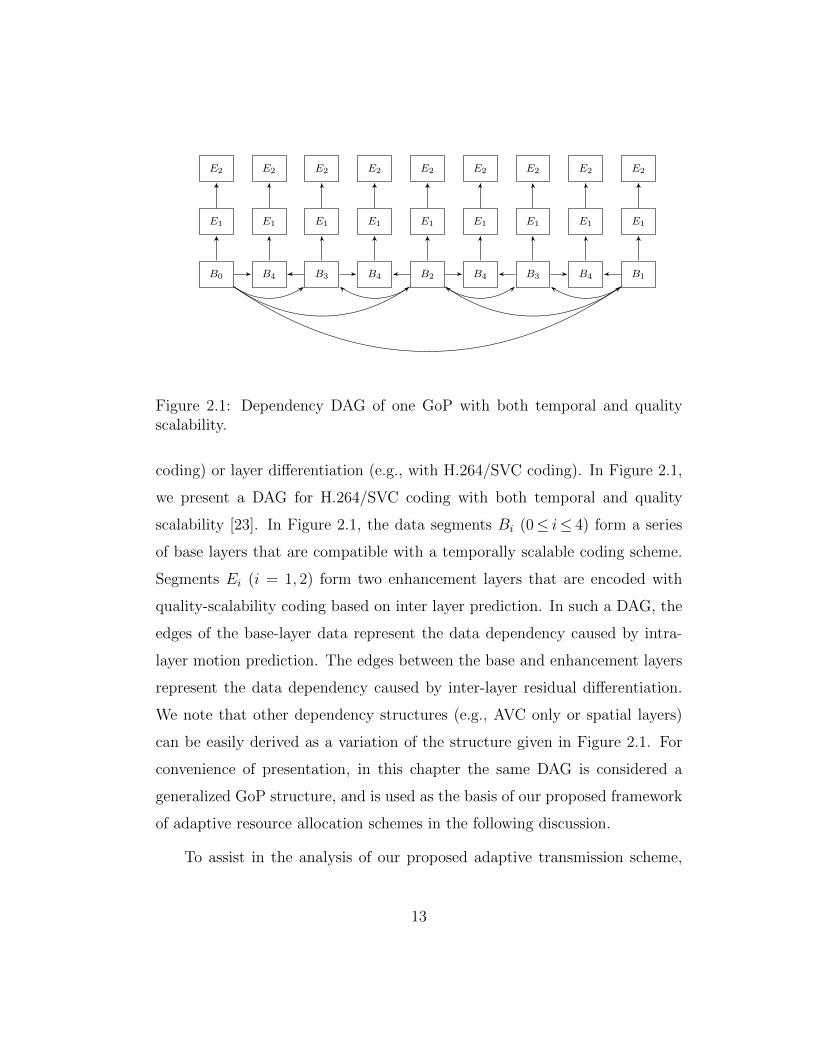
Figure 2.1: Dependency DAG of one GoP with both temporal and qualityscalability.
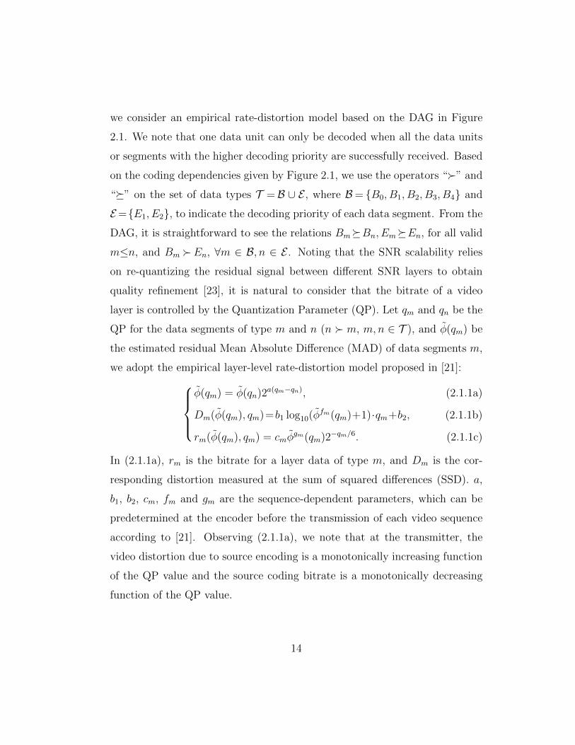
coding) or layer differentiation (e.g., with H.264/SVC coding). In Figure 2.1,
we present a DAG for H.264/SVC coding with both temporal and quality
scalability [23]. In Figure 2.1, the data segments Bi (0≤ i≤ 4) form a series
of base layers that are compatible with a temporally scalable coding scheme.
Segments Ei (i = 1, 2) form two enhancement layers that are encoded with
quality-scalability coding based on inter layer prediction. In such a DAG, the
edges of the base-layer data represent the data dependency caused by intra-
layer motion prediction. The edges between the base and enhancement layers
represent the data dependency caused by inter-layer residual differentiation.
We note that other dependency structures (e.g., AVC only or spatial layers)
can be easily derived as a variation of the structure given in Figure 2.1. For
convenience of presentation, in this chapter the same DAG is considered a
generalized GoP structure, and is used as the basis of our proposed framework
of adaptive resource allocation schemes in the following discussion.
To assist in the analysis of our proposed adaptive transmission scheme,
13
we consider an empirical rate-distortion model based on the DAG in Figure
2.1. We note that one data unit can only be decoded when all the data units
or segments with the higher decoding priority are successfully received. Based
on the coding dependencies given by Figure 2.1, we use the operators “�” and
“�” on the set of data types T =B ∪ E , where B= {B0, B1, B2, B3, B4} and
E={E1, E2}, to indicate the decoding priority of each data segment. From the
DAG, it is straightforward to see the relations Bm�Bn, Em�En, for all valid
m≤n, and Bm �En, ∀m ∈ B, n ∈ E . Noting that the SNR scalability relies
on re-quantizing the residual signal between different SNR layers to obtain
quality refinement [23], it is natural to consider that the bitrate of a video
layer is controlled by the Quantization Parameter (QP). Let qm and qn be the
QP for the data segments of type m and n (n � m, m,n ∈ T ), and φ(qm) be
the estimated residual Mean Absolute Difference (MAD) of data segments m,
we adopt the empirical layer-level rate-distortion model proposed in [21]:φ(qm) = φ(qn)2a(qm−qn), (2.1.1a)
Dm(φ(qm), qm)=b1 log10(φfm(qm)+1)·qm+b2, (2.1.1b)
rm(φ(qm), qm) = cmφgm(qm)2−qm/6. (2.1.1c)
In (2.1.1a), rm is the bitrate for a layer data of type m, and Dm is the cor-
responding distortion measured at the sum of squared differences (SSD). a,
b1, b2, cm, fm and gm are the sequence-dependent parameters, which can be
predetermined at the encoder before the transmission of each video sequence
according to [21]. Observing (2.1.1a), we note that at the transmitter, the
video distortion due to source encoding is a monotonically increasing function
of the QP value and the source coding bitrate is a monotonically decreasing
function of the QP value.
14
2.1.2 Impact of channel coding on distortion model
Since the encoded video is transmitted through an error-prone wireless channel,
it is necessary to consider the distortion introduced by error correction and
concealment. By introducing the loss probability pim when transmitting the
data of layer m in GoP i, we first ignore the details of the channel condition and
the channel coding schemes, and obtain a generalized model of the expected
distortion at the receiver. During the transmission of GoP i, if one of its base
layers m ∈ B is lost, the decoder will not be able to recover not only the frame
that layer m belongs to, but also all the lower-priority frames in the GoP. In
this situation, we assume that error concealment for a base layer is performed
using the nearest available base layer. We denote the distortion of layer m
after error concealment as Di,ecn,m, in which n represents the base layer at which
the first decoding error happens in the GoP. If we consider the general case
of transmitting layer m (m ∈ T ) in GoP i, the expected distortion of layer m
can be expressed as:
Eec{Dim} =
∑n∈B,n�m
Di,ecn,mp
in
∏j∈T ,j�n
(1− pij) + Esuc{Dim}
∏j∈T ,j�m
(1− pij).
(2.1.2)
In (2.1.2), the first term on the right-hand side accounts for the case when
the first error happens at layer n, n�m,n ∈ B. Considering that the error
propagation is confined within a GoP, we adopt the error propagation model
in [19] and obtain the following distortion model after error correction:
Di,ecn,m = pinσ
2e
1− knK−1
1 + γkn, (2.1.3)
in which K is the frame length of a GoP, kn is the frame number counted from
the first base layer of GoP i (i.e., the base layer of the I-frame) to temporal
15
layer n. σ2e and γ are the sequence/codec-determined parameters [19]. σ2
e is
the variance of the propagated error and can be treated as a constant for each
video sequence. γ is the leakage parameter that reflects the efficiency of the
spatial filtering of the encoder.
The second term in (2.1.2) accounts for the case when no error happens in
transmitting the ancestor base layers of layer m. Esuc{Dim} is the conditional
expected distortion of layer m when all its ancestor base layers are successfully
received. We can express Esuc{Dim} as follows:
Esuc{Dim} =
Di,ecm,mp
im +Di
m(1− pim), m ∈ B,∑n∈E,n�m
Dinp
in
∏j∈E,j�n
(1− pij) +Dim
∏j∈E,j�m
(1− pij), m ∈ E .
(2.1.4)
In (2.1.4), Dim is the distortion for data layer m in GoP i (see (2.1.1b)), and
Di,cem,m is the distortion after error concealment at m (see (2.1.3)). On the right-
hand side of (2.1.4), the first subexpression accounts for the case when layer m
is a base layer. The second subexpression represents the expected distortion
when layer m is an enhancement layer. The structure of the second subexpres-
sion is determined by SVC coding: if an ancestor layer n of enhancement layer
m is lost, all the subsequent layers of layer n including m will be abandoned.
2.1.3 Sub-frame level data transmission with HARQ
For video delivery over a stationary packet-lossy channel, it is sufficient to
provide a nonlinear-optimization-based rate adaption solution with the gen-
eralized rate-distortion model (2.1.1a-2.1.4). However, if the channel state is
time-varying, the details of the error correction mechanism and the channel
dynamics will significantly impact the video streaming performance. This is
because when the error protection scheme is inflexible, a change in the channel
16
state may lead to higher channel error rate and thus higher distortion due to
more frequent failure of layer segment transmission (this is reflected by (2.1.2)).
Also, when equal protection scheme is adopted, an error occurring in the base
layer will have more serious impact on the end-to-end distortion than in the
enhancement layer (see (2.1.4)). In order to tackle the first problem of channel-
error-induced distortion, we consider the scenario of a non-stationary slowly
varying channel, of which the state evolution can be modeled as a finite-state
Markov chain [24]. Considering that the hierarchy of the data unit decoding
priority is given, we adopt HARQ/FEC for unequal error protection during
video streaming.
We consider that Incremental Redundancy-HARQ (IR-HARQ)/FEC based
on a family of Rate Compatible Punctured Convolutional (RCPC) codes [24]
is adopted for channel error protection of the layer-data segments. Since the
packet length of a layer segment is much longer than the single-bit based feed-
back signals (namely, ACK and NAK), we assume that the feedback signal is
error-free and immediately ready after the transmission of each data segment.
We denote the set of channel state by Sc={s1, . . . , s|Sc|} and the RCPC coding
rate by C={c1, . . . , c|C|} (ci>cj if i<j). With RCPC coding, if a NAK is re-
ceived after the transmission with coding rate ci, the incremental redundancy
bits will be generated for retransmission by computing the residual bits be-
tween code ci and the next target code ci+1.The decoding is performed with a
Viterbi decoder that combines the previous and the current set of transmitted
bits. We assume that the channel state remains the same during transmission
round j for layer n of GoP i as sin,j. If k retransmissions are supported be-
fore the decoding deadline for layer n of GoP i, then the loss probability pin
(i.e., the probability of encountering the first error with the Viterbi decoder)
17
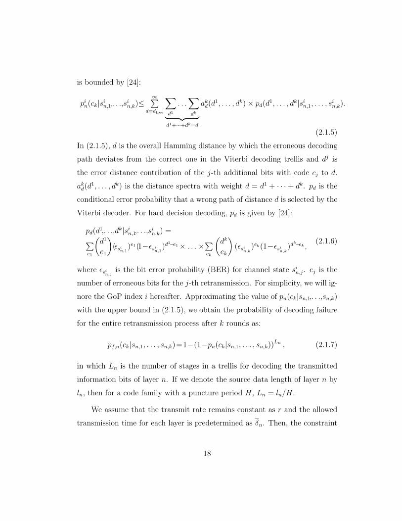
is bounded by [24]:
pin(ck|sin,1,. . .,sin,k)≤∞∑
d=dfree
∑d1
. . .∑dk︸ ︷︷ ︸
d1+···+dk=d
akd(d1, . . . , dk)× pd(d1, . . . , dk|sin,1, . . . , sin,k).
(2.1.5)
In (2.1.5), d is the overall Hamming distance by which the erroneous decoding
path deviates from the correct one in the Viterbi decoding trellis and dj is
the error distance contribution of the j-th additional bits with code cj to d.
akd(d1, . . . , dk) is the distance spectra with weight d = d1 + · · · + dk. pd is the
conditional error probability that a wrong path of distance d is selected by the
Viterbi decoder. For hard decision decoding, pd is given by [24]:
pd(d1,. . .,dk|sin,1,. . .,sin,k) =∑
e1
(d1
e1
)(εsin,1
)e1(1−εsin,1)d
1−e1× . . .×∑ek
(dk
ek
)(εsin,k
)ek(1−εsin,k)d
k−ek ,(2.1.6)
where εsin,jis the bit error probability (BER) for channel state sin,j. ej is the
number of erroneous bits for the j-th retransmission. For simplicity, we will ig-
nore the GoP index i hereafter. Approximating the value of pn(ck|sn,1,. . .,sn,k)
with the upper bound in (2.1.5), we obtain the probability of decoding failure
for the entire retransmission process after k rounds as:
pf,n(ck|sn,1, . . . , sn,k)=1−(1−pn(ck|sn,1, . . . , sn,k))Ln , (2.1.7)
in which Ln is the number of stages in a trellis for decoding the transmitted
information bits of layer n. If we denote the source data length of layer n by
ln, then for a code family with a puncture period H, Ln = ln/H.
We assume that the transmit rate remains constant as r and the allowed
transmission time for each layer is predetermined as δn. Then, the constraint
18
c1 c2 c3 cn
cT
NAK NAK NAK
ACK
ACK ACK Always
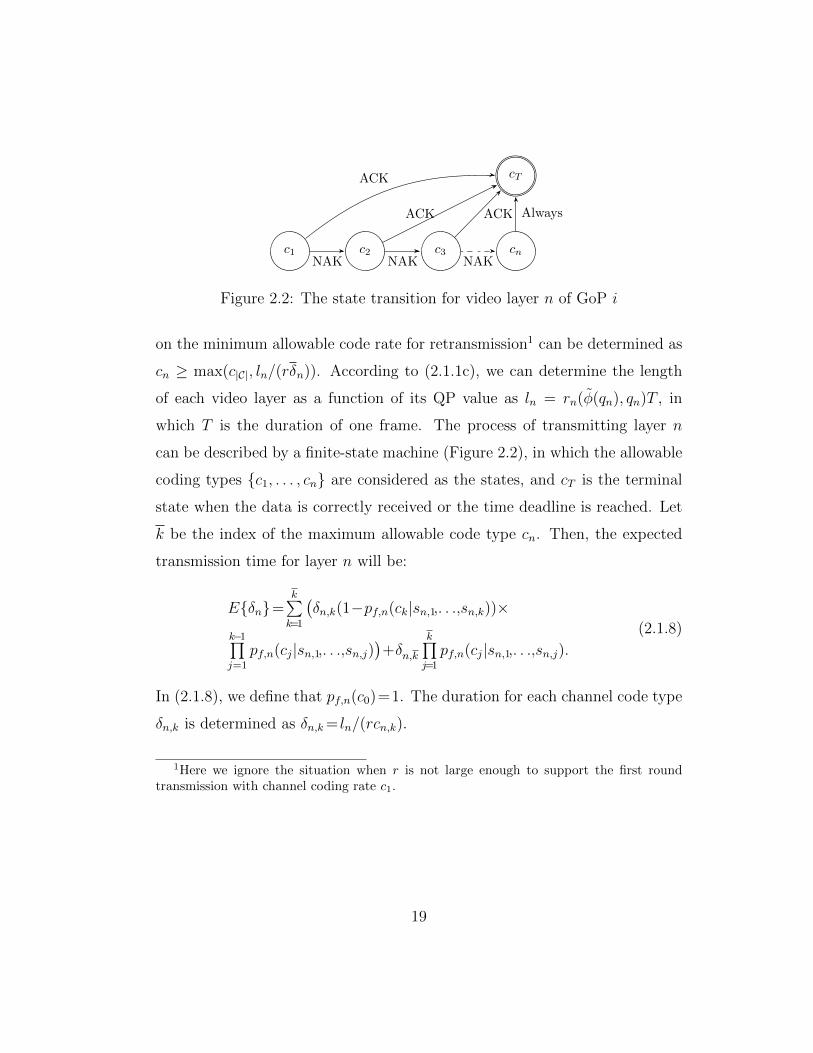
Figure 2.2: The state transition for video layer n of GoP i
on the minimum allowable code rate for retransmission1 can be determined as
cn ≥ max(c|C|, ln/(rδn)). According to (2.1.1c), we can determine the length
of each video layer as a function of its QP value as ln = rn(φ(qn), qn)T , in
which T is the duration of one frame. The process of transmitting layer n
can be described by a finite-state machine (Figure 2.2), in which the allowable
coding types {c1, . . . , cn} are considered as the states, and cT is the terminal
state when the data is correctly received or the time deadline is reached. Let
k be the index of the maximum allowable code type cn. Then, the expected
transmission time for layer n will be:
E{δn}=k∑k=1
(δn,k(1−pf,n(ck|sn,1,. . .,sn,k))×
k−1∏j=1
pf,n(cj|sn,1,. . .,sn,j))+δn,k
k∏j=1
pf,n(cj|sn,1,. . .,sn,j).(2.1.8)
In (2.1.8), we define that pf,n(c0)=1. The duration for each channel code type
δn,k is determined as δn,k= ln/(rcn,k).
1Here we ignore the situation when r is not large enough to support the first roundtransmission with channel coding rate c1.
19
2.2 Adaptive Learning for Rate Adaption
2.2.1 Transmission control as a Markov decisionprocess
With the rate-distortion model (2.1.2-2.1.4), we can describe the video stream-
ing process as a finite-state Markov process (Figure 2.3). In Figure 2.3, state
g1 accounts for the base-layer transmission stage, and state g2 accounts for the
base-layer error concealment stage. The difference between g1 and g2 is due
to the data dependency of scalability coding. This is because the decoding
error at one base layer will lead to error concealment for the subsequent lower-
priority base layers in the same GoP. Thus, the dropping of their respective
enhancement layers. In order to differentiate the base-layer types, we define g1
and g2 as a composition of the layer type and the transmission stage, namely,
g1 =(Bi, 1) and g2 =(Bi, 0) (Bi∈B). Here “1” indicates the data transmission
stage and “0” indicates the error concealment stage. In Figure 2.3, state g3
and g4 account for the transmission stage of the first and the second enhance-
ment layer, respectively. For scalability coding, lower-priority (enhancement
layer) segments will discarded whenever an error is detected during decoding
the higher-priority layer. Therefore, transition probabilities p(g2|g1), p(g1|g3)
and p(g1|g4) are equivalent to the probabilities of transmission failure in state
g1, g3 and g4, respectively. Based on the IR-HARQ scheme (2.1.5-2.1.8), these
transition probabilities are determined by the group of channel states and code
types for each layer. Noting that error propagation is confined within a single
GoP, we have p(g1|g2) = 1 and p(g2|g2) = 0 if g2 = (B4, 0) and g1 = (B0, 1),
otherwise the streaming process will stay at the error-concealment stage, g2,
so p(g1|g2) = 0 and p(g2|g2) = 1. Let sn = (sn,1, . . . , sn,k), then we can sum-
20
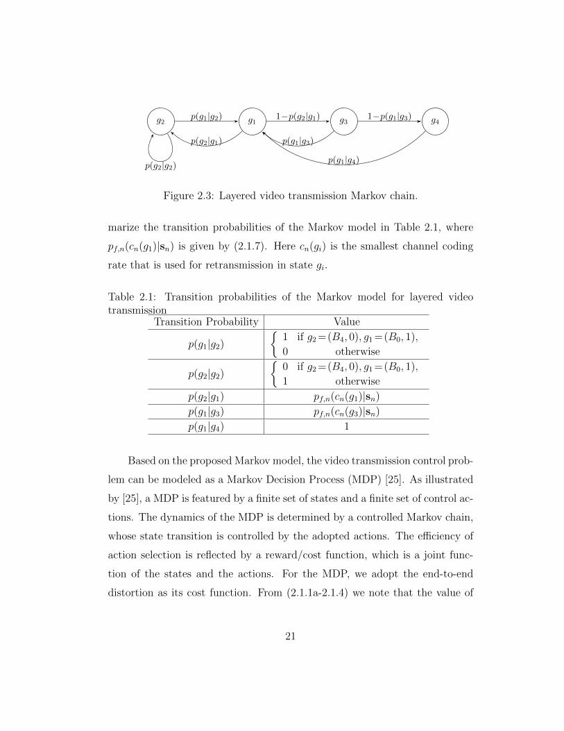
g1g2 g3 g41−p(g2|g1)
p(g2|g1)
p(g1|g2)
p(g2|g2)
1−p(g1|g3)
p(g1|g3)
p(g1|g4)
Figure 2.3: Layered video transmission Markov chain.
marize the transition probabilities of the Markov model in Table 2.1, where
pf,n(cn(g1)|sn) is given by (2.1.7). Here cn(gi) is the smallest channel coding
rate that is used for retransmission in state gi.
Table 2.1: Transition probabilities of the Markov model for layered videotransmission
Transition Probability Value
p(g1|g2){
1 if g2 =(B4, 0), g1 =(B0, 1),
0 otherwise
p(g2|g2){
0 if g2 =(B4, 0), g1 =(B0, 1),
1 otherwise
p(g2|g1) pf,n(cn(g1)|sn)
p(g1|g3) pf,n(cn(g3)|sn)
p(g1|g4) 1
Based on the proposed Markov model, the video transmission control prob-
lem can be modeled as a Markov Decision Process (MDP) [25]. As illustrated
by [25], a MDP is featured by a finite set of states and a finite set of control ac-
tions. The dynamics of the MDP is determined by a controlled Markov chain,
whose state transition is controlled by the adopted actions. The efficiency of
action selection is reflected by a reward/cost function, which is a joint func-
tion of the states and the actions. For the MDP, we adopt the end-to-end
distortion as its cost function. From (2.1.1a-2.1.4) we note that the value of
21
the cost function is controlled by the QP values and the transmission stages
(i.e., error concealment stage or data transmission stage). According to Ta-
ble 2.1, the MDP transition probabilities is a function of the channel states,
the layer types, the transmission stages and the adopted channel coding rate
for IR-HARQ. We also note from the discussion on (2.1.7) that the allowable
channel coding rate of one layer is determined by the final code type of its
previous layer. Therefore, we can model the MDP by extending the Markov
model in Figure 2.3 into a constrained controlled Markov chain. Formally, the
constrained MDP is defined as a 5-tuple {S,A, u, v,Pr}:
• S = {S1, . . . , S|S|} is the state space. S = Sc × T × I, where Sc is the
set of discretized channel states, T 3 y is the set of the layer types and
I={0, 1}3I is the set of the indicators for the transmission stages. We
note that since no error concealment is performed for the enhancement
layers, It is only valid when In=1,∀yn∈E .
• A = {a1, . . . , a|A|} is the action space. A = C × Q, in which C is the
set of the candidate RCPC code rate that can be used in the maximum
round of retransmission. Q is the set of candidate QP values that are
chosen according to the SVC coding standard.
• u = Dn(Sn, an) is the instantaneous cost function for transmitting video
layer n:
u(Sn, an) =
{Dn(sn, qn, cn), if In = 1,
Decm,n(kn(yn)), if In = 0.
(2.2.1)
In (2.2.1), the first subexpression on the right-hand side accounts for
the data transmission stages (see (2.1.4)). The second subexpression
22
accounts for the stages of error concealment of a base layer (see (2.1.3)).
m is the index of the layer used for error concealment (see (2.1.3)).
• v is the constraint on the allowable transmission time for one layer.
According to the IR-HARQ scheme (2.1.7-2.1.8), v can be expressed as
follows:
v(Sn, an)= δn(sn, qn, cn)− δn (2.2.2)
• Pr=Pr(Sn+1|Sn, an) is the transition probability of the MDP. Based on
Table 2.1, we have:
Pr(sn+1, yn+1, In+1|sn, yn, In, an)
=
pf,n(cn|sn)p(sn+1|sn), if c1 or c2,
(1−pf,n(cn|sn))p(sn+1|sn), if c3,
1, if c4, c5 or c6,
0, otherwise.
(2.2.3)
According to Table 2.1, the conditions in (2.2.3) is given as:
c1 : In = 1, In+1 = 0, yn, yn+1 ∈ B,
c2 : In = In+1 = 1, yn = E1, yn+1 ∈ B,
c3 : In = In+1 = 1, yn � yn+1,
c4 : In = In+1 = 1, yn = E2, yn+1 ∈ B,
c5 : In = 0, In+1 = 1, yn = B4, yn+1 = B0,
c6 : In = 0, In+1 = 0, yn ∈ B, yn+1 6=B0.
Here c1 and c2 account for the transmission failures in the data trans-
mission stage. c3 accounts for the transmission success. c4 and c5
account for the cases of beginning to transmit the base layer of a new
video frame. c6 accounts for the cases of self-transiting in the error
concealment stages.
23
2.2.2 Model-free learning for optimal video streamingpolicy
According to (2.2.1-2.2.3), the formulated MDP model is unichain [25]. The
goal of transmission scheduling is to find the optimal policy for the MDP that
minimizes the long-term average distortion at the receiver. We can express
the objective of the constrained MDP given by (2.2.1-2.2.3) as follows:
U = limn→∞
1
nEπ
[n∑
m=1
u(Sm, am)
], (2.2.4)
s.t. C = limn→∞
1
nEπ
[n∑
m=1
v(Sm, am)
]≤ 0,
where π is the stationary, randomized policy for taking an action a in state S:
π(a) = [Pr(a = a|S) : S ∈ S]. Using Theorems 12.7 from [25], we can obtain
the optimal policy for minimizing (2.2.4) by establishing an unconstrained
MDP through the Lagrangian approach:
U∗ = minπ
supλ≥0
J(π, λ) = supλ≥0
minπJ(π, λ), (2.2.5)
where λ is the Lagrangian multiplier and J(π, λ) is given by:
J(π, λ)= limn→∞
1
nEπ
[n∑
m=1
(u(Sm, am)+λv(Sm, am))
]. (2.2.6)
Based on (2.2.6), we can define the immediate Lagrangian cost as u(S, a, λ) =
u(S, a)+λv(S, a). According to [22], for a fixed λ there exists a value func-
tion V ∗(S, λ) for the inner problem in (2.2.5) satisfying the following Bellman
equation:
V ∗(S, λ)+J∗(λ)=mina
(u(S, a, λ)+∑S′
Pr(S ′|S, a)V ∗(S ′, λ)), (2.2.7)
24
such that the greedy policy π∗λ leads to the optimal average cost J∗ over all
possible policies π. In order to avoid the inaccuracy due to the adoption of
both the empirical distortion model and the unknown transition probabilities,
we resort to the technique of R-learning [22] to adaptively approach the value
of V ∗ and J∗ using the feedback of the immediate cost un(S, a, λ). Based
on (2.2.7), we introduce the action value function Rπ(S, a, λ) of the MDP
following policy π,
Rπ(S, a, λ) = u(S, a, λ)− Jπ(λ) +∑S′
Pr(S ′|S, a)Vπ(S ′, λ), (2.2.8)
where Vπ(S ′, λ) = minaRπ(S, a, λ), and Jπ(λ) is the average Lagrangian cost
following policy π. Based on (2.2.8), the optimal value of J∗ and Rπ∗(S, a, λ)
is learned iteratively through a two-time-scale learning process as follows [22]:
Rn+1(S, a, λ)← Rn(S, a, λ)(1− βn) + βn
(un(S, a, λ)−Jn+min
aRn(S ′, a, λ)
),
(2.2.9)
Jn+1(λ)← Jn(λ)(1− αn) + αn
(un(S, a, λ)+min
aRn(S ′, a, λ)−min
aRn(S, a, λ)
).
(2.2.10)
In (2.2.9) and (2.2.10), βn and αn (0 ≤ βn, αn ≤ 1) are the learning rate for
updating the estimated value of Rn and Jn, respectively. Usually, action explo-
ration based on Boltzmann distribution is adopted for policy learning [22]. If
so, Jn is updated only when a non-exploratory action is taken. Convergence is
guaranteed for the R-learning process given by (2.2.9-2.2.10), if the conditions∑n βn = ∞,
∑n β
2n ≤ ∞,
∑n αn = ∞,
∑n α
2n ≤ ∞ and limn→∞ αn/βn = 0
are all satisfied, and every state/action is visited infinitely often [26].
With the rightmost expression of (2.2.5), we can use a gradient-descent-
like algorithm to estimate λ∗ that satisfies the Kuhn-Tucker conditions:
λn+1 = λn + ξnC(π∗λn), (2.2.11)
25
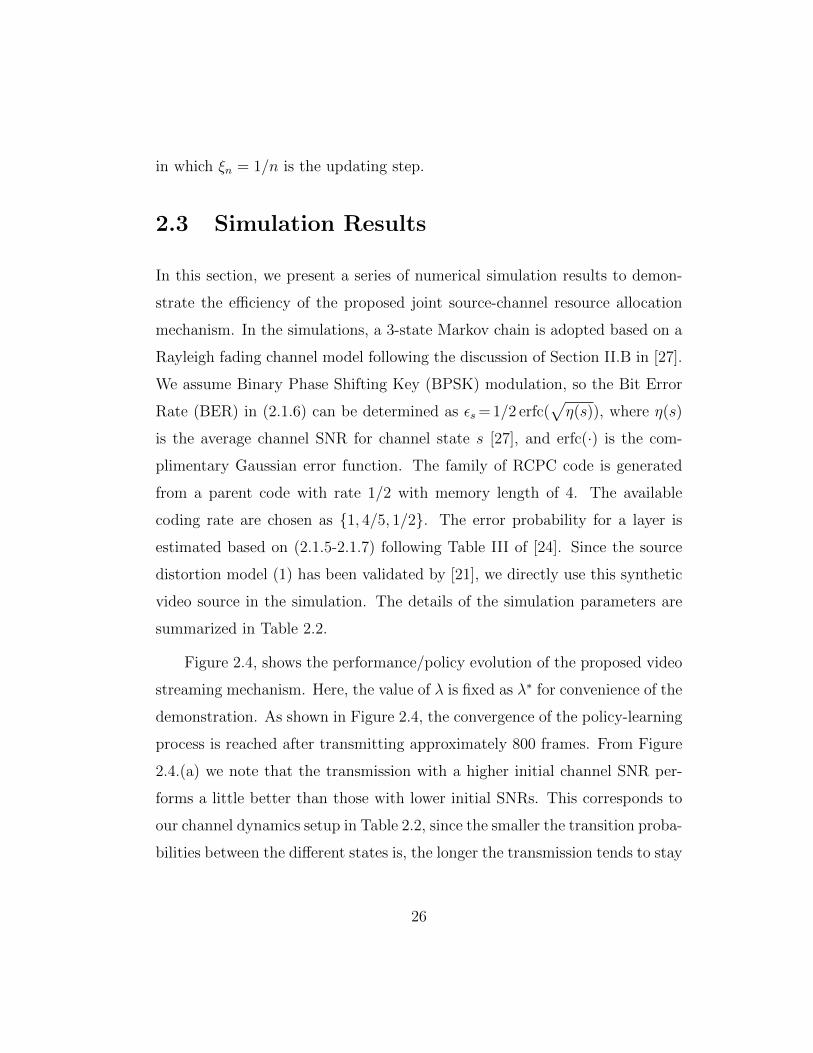
in which ξn = 1/n is the updating step.
2.3 Simulation Results
In this section, we present a series of numerical simulation results to demon-
strate the efficiency of the proposed joint source-channel resource allocation
mechanism. In the simulations, a 3-state Markov chain is adopted based on a
Rayleigh fading channel model following the discussion of Section II.B in [27].
We assume Binary Phase Shifting Key (BPSK) modulation, so the Bit Error
Rate (BER) in (2.1.6) can be determined as εs = 1/2 erfc(√η(s)), where η(s)
is the average channel SNR for channel state s [27], and erfc(·) is the com-
plimentary Gaussian error function. The family of RCPC code is generated
from a parent code with rate 1/2 with memory length of 4. The available
coding rate are chosen as {1, 4/5, 1/2}. The error probability for a layer is
estimated based on (2.1.5-2.1.7) following Table III of [24]. Since the source
distortion model (1) has been validated by [21], we directly use this synthetic
video source in the simulation. The details of the simulation parameters are
summarized in Table 2.2.
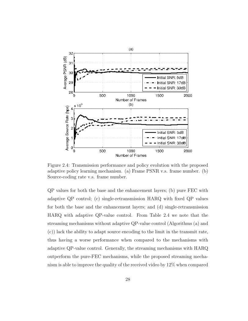
Figure 2.4, shows the performance/policy evolution of the proposed video
streaming mechanism. Here, the value of λ is fixed as λ∗ for convenience of the
demonstration. As shown in Figure 2.4, the convergence of the policy-learning
process is reached after transmitting approximately 800 frames. From Figure
2.4.(a) we note that the transmission with a higher initial channel SNR per-
forms a little better than those with lower initial SNRs. This corresponds to
our channel dynamics setup in Table 2.2, since the smaller the transition proba-
bilities between the different states is, the longer the transmission tends to stay
26
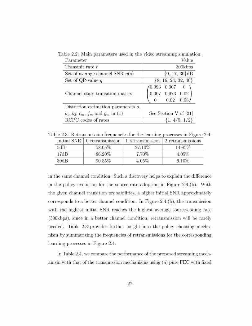
Table 2.2: Main parameters used in the video streaming simulation.Parameter Value
Transmit rate r 300kbps
Set of average channel SNR η(s) {0, 17, 30}dB
Set of QP-value q {8, 16, 24, 32, 40}
Channel state transition matrix
0.993 0.007 0
0.007 0.973 0.02
0 0.02 0.98
Distortion estimation parameters a,
b1, b2, cm, fm and gm in (1) See Section V of [21]
RCPC codes of rates {1, 4/5, 1/2}
Table 2.3: Retransmission frequencies for the learning processes in Figure 2.4.Initial SNR 0 retransmission 1 retransmission 2 retransmissions
5dB 58.05% 27.10% 14.85%
17dB 86.20% 7.70% 4.05%
30dB 90.85% 4.05% 6.10%
in the same channel condition. Such a discovery helps to explain the difference
in the policy evolution for the source-rate adoption in Figure 2.4.(b). With
the given channel transition probabilities, a higher initial SNR approximately
corresponds to a better channel condition. In Figure 2.4.(b), the transmission
with the highest initial SNR reaches the highest average source-coding rate
(300kbps), since in a better channel condition, retransmission will be rarely
needed. Table 2.3 provides further insight into the policy choosing mecha-
nism by summarizing the frequencies of retransmissions for the corresponding
learning processes in Figure 2.4.
In Table 2.4, we compare the performance of the proposed streaming mech-
anism with that of the transmission mechanisms using (a) pure FEC with fixed
27
✵ ✺✵✵ ✶✵✵✵ ✶✺✵✵ ✷✵✵✵✷�
✷✁
✸✵
✸✶
✸✷
◆✂✄☎✆✝ ✞✟ ✠✝✡✄✆☛
❆☞✌✍✎✏✌✑✒✓✔
✕✖✗✘
✭✡✙
■✚✛✜✛✡✢ ✣◆✤✥ ✺✦✧
■✚✛✜✛✡✢ ✣◆✤✥ ✶★✦✧
■✚✛✜✛✡✢ ✣◆✤✥ ✸✵✦✧
✵ ✺✵✵ ✶✵✵✵ ✶✺✵✵ ✷✵✵✵✵
✶
✷
✸
✹① ✶✵
✩
◆✂✄☎✆✝ ✞✟ ✠✝✡✄✆☛
❆☞✌✍✎✏✌✒✪✫✍✬✌✔✎✮✌✕✯✰✱✘ ✭☎✙
■✚✛✜✛✡✢ ✣◆✤✥ ✺✦✧
■✚✛✜✛✡✢ ✣◆✤✥ ✶★✦✧
■✚✛✜✛✡✢ ✣◆✤✥ ✸✵✦✧
Figure 2.4: Transmission performance and policy evolution with the proposedadaptive policy learning mechanism. (a) Frame PSNR v.s. frame number. (b)Source-coding rate v.s. frame number.
QP values for both the base and the enhancement layers; (b) pure FEC with
adaptive QP control; (c) single-retransmission HARQ with fixed QP values
for both the base and the enhancement layers; and (d) single-retransmission
HARQ with adaptive QP-value control. From Table 2.4 we note that the
streaming mechanisms without adaptive QP-value control (Algorithms (a) and
(c)) lack the ability to adapt source encoding to the limit in the transmit rate,
thus having a worse performance when compared to the mechanisms with
adaptive QP-value control. Generally, the streaming mechanisms with HARQ
outperform the pure-FEC mechanisms, while the proposed streaming mecha-
nism is able to improve the quality of the received video by 12% when compared
28
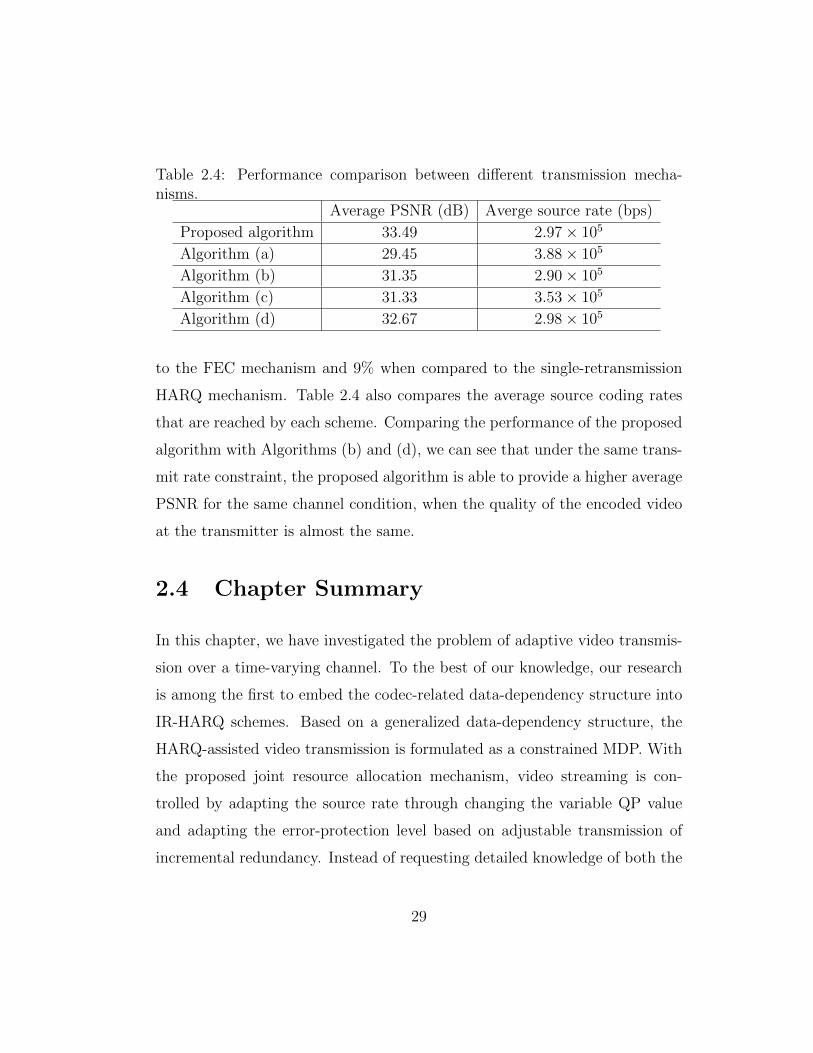
Table 2.4: Performance comparison between different transmission mecha-nisms.
Average PSNR (dB) Averge source rate (bps)
Proposed algorithm 33.49 2.97× 10⁵
Algorithm (a) 29.45 3.88× 10⁵
Algorithm (b) 31.35 2.90× 10⁵
Algorithm (c) 31.33 3.53× 10⁵
Algorithm (d) 32.67 2.98× 10⁵
to the FEC mechanism and 9% when compared to the single-retransmission
HARQ mechanism. Table 2.4 also compares the average source coding rates
that are reached by each scheme. Comparing the performance of the proposed
algorithm with Algorithms (b) and (d), we can see that under the same trans-
mit rate constraint, the proposed algorithm is able to provide a higher average
PSNR for the same channel condition, when the quality of the encoded video
at the transmitter is almost the same.
2.4 Chapter Summary
In this chapter, we have investigated the problem of adaptive video transmis-
sion over a time-varying channel. To the best of our knowledge, our research
is among the first to embed the codec-related data-dependency structure into
IR-HARQ schemes. Based on a generalized data-dependency structure, the
HARQ-assisted video transmission is formulated as a constrained MDP. With
the proposed joint resource allocation mechanism, video streaming is con-
trolled by adapting the source rate through changing the variable QP value
and adapting the error-protection level based on adjustable transmission of
incremental redundancy. Instead of requesting detailed knowledge of both the
29
channel state transition and the end-to-end distortion model, an R-learning
based model-free policy-learning scheme is introduced to adaptively learn the
resource allocation policy for both source and channel coding. The perfor-
mance of the proposed video streaming mechanism is demonstrated by simu-
lation results that show that the video quality at the receiver is improved by
12% when compared to a pure-FEC based scheme with the fixed source en-
coding QP value and 10% when compared to the single-retransmission HARQ
scheme.
30
Chapter 3
Learning for Self-organizedPower Allocation inHeterogeneous Network
As the demand for mobile data traffic continues to grow at an exponential
rate, the link efficiency of cellular networks is approaching its fundamental
limits. In urban area with densely deployed Macro Base Stations (MBS), the
gains of traditional strategies for spectrum efficiency improvement, such as
cell-splitting, is significantly reduced due to the severe inter-cell interference.
Moreover, the cost of site acquisition in a capacity limited area may also
become prohibitively expensive.
Compared with macrocell splitting, femtocells are considered an efficient
and economic solution to enhance the indoor experience of the cellular mo-
bile users in urban areas [28]. A femtocell is a low-power, short-range access
point, which can be quickly deployed by the end-users. It provides better spa-
tial reuse of the spectrum by serving the subscribers near the femtocell who
have a poorer connection with the MBS due to penetration loss. The net-
31
work topology with a hierarchical deployment of high-power macrocells and
low-power femtocells is known as a HetNet. In practice, the femtocell net-
work usually operates underlaying the macrocell network in a HetNet. This is
mainly due to the ad-hoc topology of the femtocells and the lack of coordina-
tion between the MBS deployed by an operator and the Femto Access Points
(FAPs) randomly deployed by the end users. Consequently, inter-cell/cross-
tier interference arises, and interference mitigation with limited coordination
becomes essential for preventing performance deterioration in a HetNet.
Due to the random, ad-hoc topology of the femtocells, the FAPs have to
operate in a situation of limited information exchange both across tiers (i.e.,
across macrocells and femtocells) and among the femtocells. Therefore, it is
highly desirable that the interference management of the femtocells is fully
distributed and self-organized, so that each Femtocell User (FU) is capable
of adapting its transmission to the surrounding radio environment with min-
imum information exchange. With this in mind, we study an energy-efficient
power allocation schemes for an overlay, two-tier HetNet. We note that in
the HetNet, conflict of node objectives exists across tiers since a Macrocell
User (MU) prefers that the cross-tier interference is minimized, while the FU
prefers to transmit at the best Signal-to-Interference-plus-Noise-Ratio (SINR).
Considering that private objectives contradict with each other and the means
of coordination is lacking, we resort to the game theoretic tools and model the
cross-tier, self-centric interactions between different users in the HetNet as a
non-cooperative game.
Under the framework of non-cooperative games, early studies such as [29]
have discovered that power control purely based on non-cooperative games will
lead to inefficient equilibria. In order to obtain the Pareto-preferred equilibria,
32
a number of approaches including the introduction of repetition [30] or exter-
nalities (e.g., pricing) [31,32] were adopted in previous research. As shown by
studies on non-hierarchical networks [31–33], choosing a proper pricing mech-
anisms with respect to different utility functions can be an efficient way to
determine the desired properties of the equilibria.
When it comes to resource allocation in hierarchical networks, such as
the femtocell networks and DSA-based CRNs, multi-player Stackelberg game
[34] modeling is widely preferred since it is able to reflect the hierarchy and
network ad-hoc topology [35, 36] at the same time. The Stackelberg game
is characterized by the sequential decision making (namely, follower-leader-
based strategy updating), and hence suitable for modeling the heterogeneous
user behaviors in the network. To avoid the excessive complexity in modeling
the Stackelberg game, most of the existing studies [36–38] assume complete
information in the game and favor a problem formulation which is able to
lead to a closed-form solution to the Stackelberg Equilibrium (SE). With such
assumptions, the SE is usually solved through reformulating the games as
hierarchical optimization problems.
Although the optimization-technique-based methods are able to precisely
analyze the SE properties, their scope is limited to the games where the utility
functions possess certain properties in order to guarantee the existence of a
closed-form solution. Beyond these games with special properties, a natural
idea is to resort to stochastic learning tools in repeated games for search-
ing the SEs. Based on the assumption of a discrete strategy space [39], a
body of literature on non-hierarchical networks can be found applying itera-
tive strategy-learning methods [40,41]. However, since these learning methods
assume homogeneous behaviors among the players, their application to hier-
33
archical networks is usually limited to an uniform learning model [42, 43].
In this chapter, we model the power allocation problem in a two-tier Het-
Net from the perspective of the Stackelberg game. In the proposed game
model, the MBS behaves as the leader and controls the total cross-tier inter-
ference by setting prices to each FU-FAP link. The FU-FAP links behave as
the followers and optimize their energy efficiency through interactive power al-
location. In order to design an efficient distributed, hierarchical power control
scheme with a pricing scheme, we adopt the power efficiency as the main utility
metric the FU-FAP link. We then investigate the scenarios of the continuous
and discrete power profile of the femtocells, respectively. Due to the compu-
tational complexity of obtaining the closed-form solution for the equilibrium,
we investigate the property of the proposed game in both the continuous and
discrete power profiles, and propose two self-organized strategy-learning algo-
rithms for the FU-FAP links in the follower game, respectively. We provide
a proof of convergence for the proposed learning schemes in the two follower
subgames among the FU-FAP links and propose two corresponding heuristic
algorithms to obtain the optimal MBS prices.
3.1 Network Model and QoS Metric
We consider the uplink transmission of a two-tier femtocell network with a
single MBS and K FAPs. The MBS and the FAPs share the same bandwidth
W and each of the FAPs is scheduled to serve one single user at each time
instance. The MBS requires that the femtocell-to-macrocell interference is
kept to an acceptable level. Due to the ad-hoc topology of the femtocells, we
assume that the information exchange only happens between the MBS and
34
FAPs. For analytical tractability, we suppose that all the channels involved
are block-fading and remains constant during each transmission block.
In what follows, we let 0 denote the index of the MU-MBS pair and k ∈
K = {1, . . . , K} denote the index of a FU-FAP pair. The channel power gain
between transmitter i and receiver j is denoted by hi,j, where i, j ∈ K⋃{0}.
The power of transmitter k is denoted by pk and the power vector of all the
FUs is denoted by p = [p1, . . . , pk]. The noise variance for the transmitter-
receiver pair k is denoted by Nk. Then the SINR level at the MBS can be
expressed as:
γ0(p0,p) =h0,0p0
N0 +∑k∈K
hk,0pk, (3.1.1)
and the SINR level at the k-th FAP can be expressed as
γk(p0,p) =hk,kpk
Nk + h0,kp0 +∑
j∈K\{k}
hj,kpj. (3.1.2)
During the operation, it is usually beneficial to shift some calls served by
the MBS to the FAP. Therefore, we suppose that for the MBS, the require-
ment on the femtocell-to-macrocell interference is not rigid. Instead, the MU
transmit with a fixed power and to control the interference level, the MBS
charges each FU-FAP link for causing interference with a certain price. We
denote the vector of interference prices at a time interval by λλλ= [λ1, . . . , λK ],
in which λk is the price for unit interference caused by FU k. The goal of the
MBS is to maximize the total revenue of collected payments from the FU-FAP
links:
maxλλλ
(u0 =
∑k∈K
λkhk,0pk
). (3.1.3)
35
For simplicity, in what follows we use the terms FU and the FU-FAP link
interchangeably. For the FUs, we assume that each local transmit power pk
is limited by the physical constraint pk ∈ [0, pmaxk ]. The goal of FU k is to
maximize its local net payoff by adapting pk:
max0≤pk≤pmax
k
(uk = ψ(γk, pk)− λshk,0pk
), (3.1.4)
in which ψ(γk, pk) is the utility function of FU k. We consider that for each FU,
the energy efficiency, namely, the data received per unit energy consumption,
is adopted as the the local utility:
ψ(γk,pk) =W log(1 + γk)
pk + pa, (3.1.5)
where pa denotes the additional circuit power consumption by FU k. We
assume that the local SINR γk can be perfectly measured at the FAP. For the
proposed femtocell network, we suppose that the following assumptions hold:
i) pk is significantly greater than pa;
ii) The femtocell-to-femtocell interference is sufficiently small.
Assumption i) is based on the fact that most power is consumed during opera-
tion by the amplifier and the radio transceiver [44]. Assumption ii) is based on
the facts that (a) the FAPs are of low transmit power and the peak transmit
power is limited; and (b) the inter-cell path loss between femtocells are usually
large, since the indoor penetration loss is usually significant. Based on these
two assumptions, we assume that the SINR constraint for a FU-FAP link is
negligible.
36

3.2 Power Allocation Based on Continuous
Stackelberg Game
We model the user interactions in the proposed network as a hierarchical game
with the MBS and the FU-FAP links choosing their actions in a sequential
manner. When the power allocation of the FUs are given as p, we can define
the leader game from the perspective of the MBS as:
Gl = 〈ΛΛΛ, {u0(λλλ,p)}〉, (3.2.1)
where the MBS is the only player of the game and the action of the player is
the price vector λλλ ∈ ΛΛΛ.
When the leader action is given by λλλ, we can define the non-cooperative
follower game from the perspective of the FUs as:
Gf = 〈K,P , {uk(λλλ,pk,p−k)}k∈K〉, (3.2.2)
where FU k is one player with the local action pk ∈ Pk.
With each player behaving rationally, the goal of the game (3.2.1) and
(3.2.2) is to finally reach the Stackelberg Equilibrium (SE) where both the
leader (MBS) and the followers (FUs) have no incentive to deviate. We first
assume that the strategies of the FUs and MBS are continuous. Then the SE
of the game can be mathematically defined as follows:
Definition 3.2.1 (Stackelberg Equilibrium). The strategy (λλλ∗,p∗) is an SE
for the proposed Stackelberg game described by (3.2.1) and (3.2.2) if
u0(λλλ∗,p∗)≥u0(λλλ,p∗),∀λλλ∈ΛΛΛ, (3.2.3)
uk(λλλ∗,p∗k,p
∗−k)≥uk(λλλ∗,pk,p∗−k),∀k ∈ K, ∀pk ∈ Pk. (3.2.4)
37
3.2.1 Femtocell power allocation with continuousstrategies
We start the analysis of the Stackelberg game in (3.2.1) and (3.2.2) by back-
ward induction. Suppose that the MBS first sets its strategy as λλλ, then we
obtain the non-cooperative follower subgame described by (3.2.2). In order
to show the existence of a pure-strategy Nash Equilibrium (NE) in Gf , we
introduce the concept of supermodular game as follows:
Definition 3.2.2 (Supermodularity [34]). A function f : X × T → R is said
to have increasing differences (supermodularity) in (x, t) if for all x′ ≥ x and
t′ ≥ t,
f(x′, t′)− f(x, t′) ≥ f(x′, t)− f(x, t).
Definition 3.2.3 (Supermodular game [34,45]). A general normal-form game
〈N , {Si}i∈N , {ui}i∈N 〉 is a supermodular game if for any player i ∈ N ,
i) the strategy space Si is a compact subset of RK.
ii) the payoff function ui is upper semi-continuous in s = (si, s−i).
iii) ui is supermodular in si and has increasing difference between any com-
ponent of si and any component of s−i.
To show that the proposed follower subgame (3.2.2) is a supermodular
game, we introduce Lemma 3.2.1 from [45]:
Lemma 3.2.1. If a function f(s) is twice differentiable, then supermodularity
is equivalent to ∂2f(s)∂si∂sj
≥ 0 ∀si, sj, j 6= i.
Based on Lemma 3.2.1, the supermodular property of the proposed fol-
lower subgame (3.2.2) is given by Theorem 3.2.1.
38
Theorem 3.2.1. Given the strategy λλλ of the MBS, the follower subgame
(3.2.2) is a supermodular game if γk ≥ pa/pk.
Proof. The first and the second conditions of a supermodular game in Defini-
tion 3.2.3 (trivially) holds for the proposed follower subgame (3.2.2). Then,
Theorem 3.2.1 can be derived based on Lemma 3.2.1. By taking the component-
wise derivative of uk(pk,p−k) with respect to pk, we obtain:
∂uk∂pk
=−W log(1+γk)
(pk+pa)2+
WGk
(1+γk)(pk+pa)−λkhk,0, (3.2.5)
in which
Gk =hk,k
N0 + h0,kp0 +∑
i∈K\{k} hi,kpi. (3.2.6)
Then ∀k, j ∈ K, k 6= j, the value of ∂2uk∂pk∂pj
is given by:
∂2uk∂pk∂pj
=WHkpk
(1+γk)(pk + pa)2+
WHkγk(1+γk)2(pk + pa)
− WHk
(1+γk)(pk + pa), (3.2.7)
in which
Hk =hj,khk,k(
N0 + h0,kp0 +∑
i∈K\{k} hi,kpi
)2 . (3.2.8)
It is easy to verify from (3.2.7) that ∂2uk∂pk∂pj
≥ 0 if γk ≥ pa/pk. By Lemma
3.2.1, uk has increasing difference between pk and any component of p−k if
γk ≥ pa/pk. By Definition 3.2.3, the proof of Theorem 3.2.1 is completed.
Given the opponent power allocation p−k, we define the local Best Re-
sponse (BR) of FU k by
pk(p−k) = arg max0≤pk≤pmax
k
(uk = ψ(γk, pk)− λshk,0pk
). (3.2.9)
Then, Theorem 3.2.1 immediately yields Proposition 3.2.1 [45]:
39

Proposition 3.2.1. At least one pure-strategy NE exists in the follower sub-
game (3.2.2) and the following hold:
i) The set of NEs (3.2.4) has the component-wise greatest element p∗ and
least element p∗.
ii) If the BRs are single-valued, and each FU uses the BR starting from the
smallest (largest) elements of the strategy space to update their strategies,
then the strategies monotonically converge to the smallest (largest) NE.
iii) If the game has a unique NE, then with any arbitrary initial strategy, the
local myopic BRs converges to the NE.
The properties of Gf given by Proposition 3.2.1 sheds light on the solution
to the local strategy-learning scheme for the FUs. To take advantages of
these properties, we introduce the concept of superlevel set and quasiconcavity
from [46]:
Definition 3.2.4 (Superlevel Set [46]). Let D denote a convex set in Rn and
f : D → R. The superlevel set of f is defined as Cf (α) = {x ∈ D|f(x) ≥ α}.
Definition 3.2.5 (Quasi-Concavity [46]). Following the notation in Definition
3.2.4, function f is quasi-concave on D if ∀α, Cf (α) is a convex set.
For conciseness, the readers are referred to Sections 3.1 and 3.4 of [46] for
more details on the definitions of superlevel set and (strict) quasiconcavity.
From [46] we further introduce Lemma 3.2.2, which implies the uniqueness of
the optimization solution to a strict quasi-concave function:
40
Lemma 3.2.2. Suppose f : D → R be strictly quasiconcave where D ⊂ RN is
convex. Then, any local maximum of f on D is also a global maximum of f
on D. Moreover, the set arg max{f(x)|x ∈ D} is either empty or a singleton.
Based on Lemma 3.2.2, we are ready to examine the BRs in Gf and obtain
Lemma 3.2.3:
Lemma 3.2.3. Given the MBS strategy λλλ, uk is strictly quasiconcave and the
best-response pk is single-valued for each FU.
Proof. The proof of Lemma 3.2.3 is derived from investigating the quasicon-
cavity of the FU payoff functions. In order to prove Lemma 3.2.3, we first
show that the utility function uk in Gf is quasiconcave. We examine the α-
superlevel set of uk(pk, p−k) in pk, which is equivalent to the 0-superlevel set
of fα(pk, p−k):
Pk,0 ={pk∣∣fα(pk, p−k) ≥ 0, 0 ≤ pk ≤ pmax
k ,
fα(pk, p−k)=W log(1+γk)−(λkhk,0pk + α)(pk + pa)}.
(3.2.10)
We note that fα(pk, p−k) is a concave function, so Pk,α is convex from the
definition of convexity. By the definition of quasiconcavity, ui(λλλ∗, pk, p−k) is
quasiconcave in pk.
Then, we show that ui(pk, p−k) is strictly quasiconcave in pk so the BR
is a global maximum and thus single-valued. Without loss of generality, we
consider the power allocation pk ∈ [0, pmaxk ] with uk(pk, p−k) = α. We assume
that a different power allocation pk satisfies uk(pk, p−k)≥ uk(pk, p−k). Corre-
spondingly, fα(pk, p−k) = 0 and fα(pk, p−k)≥0. Note that for fα(pk, p−k) = 0,
we have:
W log(1 +Gkpk) = (λshk,0pk + α)(pk + pa), (3.2.11)
41
in which Gk is given in (3.2.6). The right-hand side of (3.2.11) is a strictly in-
creasing concave function and the left-hand side is a strictly increasing convex
function in [0, pmaxk ]. Then the solution to fα(pk, p−k)=0 is unique in [0, pmax
k ],
so fα(pk, p−k)>fα(pk, p−k). Based on the definition of concave function, the
following inequality also holds for 0 < δ < 1:
fα(δpk + (1− δ)pk) ≥ δfα(pk) + (1− δ)fα(pk)
> fα(pk) = 0.(3.2.12)
Therefore, the condition for strict quasiconcavity holds as uk(δpk+(1−δ)pk) >min (uk(pk, p−k), uk(pk, p−k)) = α. Then, Lemma 3.2.3 is a direct conclusion
based on Lemma 3.2.2.
Based on Lemma 3.2.3, we can further prove that the BR of FU k has the
following properties, and therefore is a standard function [34]:
i) positivity: pk > 0,
ii) monotonicity: for any p′−k, p−k ∈ P−k, if p′−k > p−k, then pk(p′−k) ≥
pk(p−k),
iii) scalability: ∀α > 1, αpk(p−k) > pk(αp−k).
For a non-cooperative game whose best-response functions are standard
functions, we have the following property in Lemma 3.2.4 [34]:
Lemma 3.2.4. If the best-response functions of a non-cooperative game G are
standard functions for all the players, then the game has a unique NE in pure
strategies.
By checking the aforementioned properties of a standard function in the
follower subgame, we can directly apply Lemma 3.2.4 and deduce the unique-
ness of the pure-strategy NE in subgame Gf as Theorem 3.2.2:
42
Theorem 3.2.2. Given any MBS strategy λλλ, the follower subgame (3.2.2) has
a unique NE if the following condition is satisfied
hk,kpkNk + h0,kp0 +
∑j∈K hj,kpk
≥ papk. (3.2.13)
Proof. Observing (3.1.5), we note that the maximum net-payoff function is
lower-bounded by 0 with pk=0. Since the power vector is always nonnegative,
the positivity property in the BR for each FU k immediately follows Lemma
3.2.3.
We denote Ik(p−k)=(Nk+h0,kp0+∑
j∈K\{k} hj,kpj)/hk,k. Noting that Ik(p−k)
is a strictly increasing function of p−k, monotonicity of pk(p−k) can be illus-
trated by proving that function pk(Ik) is monotonically increasing in Ik. From
(3.2.5) we obtain the necessary condition for pk to be the BR as ∂uk∂pk
= 0, which
is equivalent to
ω(pk, Ik) =W (pk + pa)
Ik−W (1 +
pkIk
) log(1 +pkIk
)
− λkhk,k(pk + pa)2(1 +
pkIk
) = 0. (3.2.14)
Since ∂pk∂Ik
= − ∂ω∂Ik/ ∂ω∂pk
, we have
∂ω
∂Ik=
1
I2k
(ξ(pk)+Wpk log(1+
pkIk
)−Wpa
), (3.2.15)
where ξ(pk) = λkhk,k(p2apk + 2pap
2k + p3k), and
∂ω
∂pk= − 1
Ik
(ζ(pk) +W log(1+
p
Ik)
)(3.2.16)
where ζ(pk) = λkhk,k(pa+pk)(pa+2Ik+3pk). We note that ∂ω∂pk
< 0, then the
property of monotonicity holds iff ∂ω∂Ik≥ 0. With the inequality of logarithmic
function given in [47], log(1 + x) ≥ x/(1 + x) for x ≥ −1, we obtain,
∂ω
∂Ik≥ 1
I2k
(ξ(pk)+
W
Ik + pk
(p2k − pa(Ik + pk)
)). (3.2.17)
43
Therefore, ∂pk∂Ik≥ 0 if p2k − pa(Ik + pk) ≥ 0. Then, we obtain the condition for
pk(p−k) to be monotonic as:
hk,kpkNk + h0,kp0 +
∑j∈K hj,kpk
≥ papk. (3.2.18)
The proof of scalability is based on Lemma 3.2.3. According to Lemma
3.2.3, there is a one-to-one correspondence between pk and γk. We define
Jk(p−k) =∑
j∈K\{k} hj,kpj, then from (3.1.2) the BR can be written as
pk(p−k) =γk (N0 + h0,kp0 + Jk(p−k))
hk,k. (3.2.19)
From ∂uk∂pk
= 0, we can prove that ∂γk∂Jk≤ 0 following the same procedure as
for proving monotonicity (which is omitted for conciseness). Therefore, γk
is a decreasing function of Jk. Since Jk(p−k) is a standard function [45], we
realize that if α > 1, γk(αp−k) ≤ γk(p−k) and Jk(αp−k) ≤ αJk(p−k). Then,
monotonicity holds for pk(p−k) since
pk(αp−k) ≤γk(p−k) (N0+h0,kp0+αJk(p−k))
hk,k≤ αpk(p−k). (3.2.20)
Therefore, pk(p−k) is a standard function. Based on Lemma 3.2.4, we conclude
that the NE of the follower subgame (3.2.2) is unique.
Remark 3.2.1. If in subgame Gf the condition of Theorem 3.2.2 is satisfied,
the condition of Theorem 3.2.1 will also be satisfied. Equation (3.2.13) in-
dicates that to ensure the uniqueness of the NE, the SINR of a FU should
be significantly greater than the ratio between its transmit power and circuit
power. Such a condition is guaranteed by our assumption of the network in
Section 3.1.
44
We assume that the channel power gain hk,0 is known and the SINR γk can
be perfectly measured by each FAP. Then, based on Lemma 3.2.3, pk can be
solved locally with the bisection method [46]. Based on Proposition 3.2.1 and
Theorem 3.2.2, the asynchronous strategy-updating mechanism defined in [45]
can be directly applied to Gf . By Proposition 3.2.1, the convergence to the NE
is guaranteed from any arbitrary initial power vector. The strategy-learning
algorithm is summarized as Algorithm 3.1:
Algorithm 3.1 Asynchronous strategy updating
Require: each FU sets up an infinite increasing time sequence {T ik}k∈K forscheduling strategy update.
1: for all t ∈ {T ik}k∈K do2: for all k s.t. t = {T ik} do3: given pt−1−k , obtain ptk = pk(p
t−1−k ) as in (3.2.9) with bisection.
4: end for5: end for
3.2.2 Approximate solution to the price of MBS
Now we assume that the strategies of the FUs are given as p from (3.2.9) and
consider the leader subgame Gl. For the subgame given by (3.2.1), the local
BR is given by (cf. (3.1.3))
λλλ = arg maxλλλ�0
(∑k∈K
λkhk,0pk
). (3.2.21)
To investigate the solution of (3.2.21), we first consider the feasibility
region for λk. We note from (3.2.9) that the maximum value of uk is lower-
bounded by 0 (when pk=0) and upper-bounded by ψ(γk, pk), where (γk, pk) =
arg maxψ(γk, pk). Thereby, the price λk charged by the MBS is also upper-
bounded. Otherwise, if λk is too high (i.e., making ψ(γk, pk)<λshkpk), FU k
45
will stop transmitting and be forced out of the power allocation game. With
the aforementioned bound on uk, we look for the constraint on λk in (3.2.9).
However, since uk in (3.2.9) is a transcendental function, it is difficult to de-
rive a closed-form expression of the constraint on λk. Then, the challenge in
analyzing Gl is to find an efficient way to obtain the optimal price λλλ.
By jointly investigating the leader and the follower subgames, we can show
that a finite, optimal price λk for each FU coexists with the NE of the follower
subgame.
Theorem 3.2.3. In the Stackelberg game defined by (3.2.1) and (3.2.2), there
exists at least one pure-strategy SE with finite price vector λλλ from the leader
game.
Proof. The proof is based on Theorem 3.2 of [34]. The existence of a pure-
strategy SE is guaranteed when each local strategy in the game is compact
and convex and the corresponding payoff function is quasiconcave. For the
FUs, quasiconcavity of uk(p,λλλ) in pi is given by Lemma 3.2.3. For the MBS,
u0 is an affine function of λλλ, hence it is quasiconcave in λλλ. It is trivial that
p and λλλ are convex and compact, then based on Theorem 3.2 of [34], there
exists a pure-strategy NE in the game. Based on our discussion after (3.2.21)
on the fact that 0 ≤ λk <∞, we can derive the relationship between the BRs
of the FUs and the MBS from ∂uk∂pk
= 0 as:
λk =WGk
hk(1 + γk)(pk + pa)− W log(1 + γk)
hk(pk + pa)2, (3.2.22)
where pk and γk are the local BR and the corresponding SINR. Gk is given
by (3.2.6) in the proof of Theorem 3.2.1. For (3.2.22), the value of the right-
hand side expression is upper-bounded since 0 ≤ pk ≤ pmaxk . Therefore, λk is
finite.
46
Our approximate solution to the leader subgame is inspired by the pio-
neering work [31], which models the asymptotic behaviors of the equilibrium
power vector and the corresponding payments. We assume that each FU’s
behavior can be asymptotically modeled by two regions, the price-insensitive
region and the price-sensitive region. In the price-insensitive region, the FU’s
behaviors are hardly influenced by the price. In the price-sensitive region, the
local power allocation pk is driven toward 0. We note that the necessary condi-
tion for the NE of the FUs is given by (3.2.22). As λk → 0, the solution of the
BRs in the follower game will be independent of λk and can be approximated
by
(1 + γk) log(1 + γk)−Wγk −WGkpa = 0, k ∈ K, (3.2.23)
where Gk is given by (3.2.6). From Lemma 3.2.3, the solution to (3.2.23) is
unique. Then the payment by FU k will be a linear function of λk, rk =
hk,0pkλk.
On the contrary, as λk →∞, ∀k ∈ K, pk → 0. From (3.2.22) we obtain:
hk,kλk(pk + pa)=Whk,k
Ik+ hk,kpk−W log(1 +
hk,kpkIk
)
(pk + pa), (3.2.24)
where Ik is the sum of interference plus noise defined in the proof of Theorem
3.2.2. With pk → 0,∀k, (3.2.24) can be approximated as:
hk,kλk(pk + pa)≈Whk,k
Nk + h0,kp0. (3.2.25)
and from (3.2.25) we obtain
pk≈W
λk(Nk + h0,kp0)− pa. (3.2.26)
Based on (3.2.23) and (3.2.26) we obtain the following two-region asymp-
totic models for the FU behaviors:
47
• Low-price asymptote as λk → 0:{γ∗k ≈ γk,
rk(λk, pk) = hk,0pkλk ∝ λk.(3.2.27)
• High-price asymptote as λk →∞:
pk≈W
λk(Nk + h0,kp0)− pa. (3.2.28)
In (3.2.27), γk is the equilibrium SINR when λk = 0. Since in the low-price
asymptote, rk increases with λk and in the high-price asymptote it decreases
with λk, the maximum payment must happen between the two regions. Then,
we can extend the two FU payment asymptotes toward each other until they
meet at the intersection price λak. With such an approximation, rk(λak, pk)
will be the maximum payment received from FU k. Combining (3.2.27) and
(3.2.28), we can obtain the intersection point for the two asymptotes as:
λak ≈W
(p∗k + pa)(N + h0,kp0), (3.2.29)
where p∗k is the power allocation corresponding to the SINR γ∗ in (3.2.27).
γ∗ can be obtained by setting λλλ = 0 and solving (3.2.23) with the BR-based
asynchronous strategy-updating mechanism.
3.3 Learning for Power Allocation in
Discrete Stackelberg Game
In this section, we extend the analysis of the Stackelberg game described by
(3.2.1) and (3.2.2) to a more practical scenario where the FUs choose their
transmission strategies from a finite, discrete set of powers. In this case, the
conditions for the existence of NEs in the continuous game (i.e., Theorems
48
3.2.2 and 3.2.3) are not satisfied anymore. Therefore, the properties of the
game need to be re-evaluated. Within the same game structure for (3.2.1) and
(3.2.2), we denote the discrete action set of the FUs by Pk={p1k=0, . . . , p|Pk|k }.
It is well known that every finite non-cooperative game has a mixed-strategy
NE [34]. For the follower subgame, we define the mixed-strategies of FU k
as πππk = [π1k, . . . , π
|P|k ], where πjk(p
jk) = Pr(pk = pjk) is the probability for FU k
to choose the j-th action pjk ∈ Pk. Then, given any MBS price λλλ, there will
be at least one mixed-strategy NE for the FUs. Different from the previous
continuous game, the expected net payoff for FU k becomes
uk(πππk,πππ−k,λλλ)=∑p∈P
(ψk(pk, p−k)−λkhk,0pk)∏i∈K
∏1≤j≤|Pk|
πji , (3.3.1)
where∑
j πjk = 1, 0 ≤ πjk ≤ 1. Similarly, the expected revenue of the MBS
becomes
u0(λλλ,πππ) =∑k∈K
λk∑
1≤j≤|Pk|
πjkhk,0pjk. (3.3.2)
Due to the limit on information exchange, FU k can only attain its local
payoff uk(pjk,πππ−k) each time when it chooses pjk and the other FUs adopt
the mixed strategies πππ−k. To ensure that each FU is able to learn its Nash
distribution πππk, we adopt the Logit best response function (namely, the smooth
BR based on entropy perturbation) [48]:
βtk(pjk|πππ−i)=
exp(U t−1k (pjk,πππ−k)/τ)∑
1≤i≤|Pk| exp(U t−1k (pik,πππ−k)/τ)
, (3.3.3)
where U tk is the estimated expected payoff at time t. τ is a positive scalar (also
known as Boltzmann temperature) that controls the sensitivity of the BR to
perturbation.
49
Based on the two-timescale strategy learning scheme [48], we introduce
two coupled stochastic learning processes to approximate Uk(pjk) and πk(p
jk) in
(3.3.3) as,
U tk(p
jk)=U t−1
k (pjk)+αt11(πjk(p
jk))
(utk(p
jk)−U
t−1k (pjk)
), (3.3.4)
πtk(pjk)=πt−1k (pjk)+αt2
(βtk(p
jk|πππ−i)− π
t−1k (pjk)
). (3.3.5)
In (3.3.4) and (3.3.5), utk(pjk) is the instant payoff observation at the FAP
in (3.1.5) and βtk(pjk|πππ−i) is the smooth BR given in (3.3.3). 1(πj
k(pjk))
is the
indicator function. 1(πjk(p
jk))
= 1 if πjk(pjk) = 1 and otherwise 1(πj
k(pjk))
= 0. The
parameter sequence αt1 and αt2 satisfy the following conditions:limT→0
T∑t=1
αt1 = +∞, limT→0
T∑t=1
(αt1)2 < +∞,
limT→0
T∑t=1
αt2 = +∞, limT→0
T∑t=1
(αt2)2 < +∞,
limt→0
αt2
αt1
= 0.
(3.3.6)
The conditions in (3.3.6) ensures that the learning of strategies changes on a
slower timescale than that of the action values. Based on Lemma 3.3.1 and
Lemma 3.3.2 given in [49], we can show in Theorem 3.3.1 that the proposed
learning processes in 3.3.3-3.3.6 converges.
Lemma 3.3.1. Consider game G with payoff function uk(s) for player k. If
the sequence of stochastic fictitious play converges, it also holds for game Gwith payoff function uk(s) = κkuk(s)+ϑ(sk), in which κk is a positive constant
and ϑ(sk) only depends on player k’s own behavior.
Lemma 3.3.2. Consider stochastic fictitious play starting from any arbitrary
πππ0. If G is a supermodular game, then
Pr(ω{πππ0k} ⊂ RP or ω{πππ0
k} ⊂Mi ∩ [πππk,πππk] for k) = 1
50
where ω{πππ0k} is an invariant set of the solution trajectory starting from πππ0
k. RP
is the set of rest points (fixed points) and πππk,πππk ∈ RP such that RP ⊂ [πππk,πππk].
Mi is a finite Lipschitz submanifold and every persistent non-convergence tra-
jectory is asymptotic to one in Mi.
Theorem 3.3.1. With any arbitrary πππ0 and U0k , the strategy-learning mecha-
nism (3.3.3)-(3.3.5) almost surely converges to some fixed point if conditions
in (3.3.6) are satisfied. The probability of converging to a NE is non-zero.
Proof. The proof of Theorem 3.3.1 starts by investigating the supermodularity
property in the FU subgame. With a discrete power set, the expected payoff
function (3.3.1) can be rewritten as:
uk(πππk,πππ−k,λλλ)=∑p∈P
ψk(pk, p−k)∏i∈K,j
πji −∑j
λkhk,0pjkπ
jk, (3.3.7)
which is in the form uk(πππ)=κkuk(πππ)+ϑ(πππk) with κk=1. By Lemma 3.3.1, we
only need to check the game with payoff
uk(πππk,πππ−k,λλλ)=∑p∈P
ψk(pk, p−k)∏i∈K,j
πji . (3.3.8)
With Definition 3.2.3 and Lemma 3.2.1, it is easy to check that the game with
payoff function (3.3.8) and mixed strategies is a supermodular game. Based
on Theorem 6 of [48], the process of πtk produced by (3.3.3)-(3.3.5) will almost
surely be an asymptotic pseudotrajectory of the smooth BR dynamics:
πk = βk(πππ−k)− πk.
Then, based on Lemma 3.3.2, for the game with payoff (3.3.8), the stochastic
fictitious play almost surely converges with any arbitrary initial πππ0. Follow-
ing Lemma 3.3.1, convergence holds for the original subgame with payoff uk,
proving Theorem 3.3.1.
51
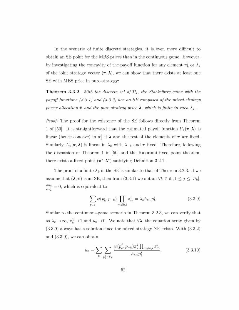
In the scenario of finite discrete strategies, it is even more difficult to
obtain an SE point for the MBS prices than in the continuous game. However,
by investigating the concavity of the payoff function for any element πjk or λk
of the joint strategy vector (πππ,λλλ), we can show that there exists at least one
SE with MBS price in pure-strategy:
Theorem 3.3.2. With the discrete set of Pk, the Stackelberg game with the
payoff functions (3.3.1) and (3.3.2) has an SE composed of the mixed-strategy
power allocation πππ and the pure-strategy price λλλ, which is finite in each λk.
Proof. The proof for the existence of the SE follows directly from Theorem
1 of [50]. It is straightforward that the estimated payoff function Uk(πππ,λλλ) is
linear (hence concave) in πik if λλλ and the rest of the elements of πππ are fixed.
Similarly, U0(πππ,λλλ) is linear in λk with λ−k and πππ fixed. Therefore, following
the discussion of Theorem 1 in [50] and the Kakutani fixed point theorem,
there exists a fixed point (πππ∗,λλλ∗) satisfying Definition 3.2.1.
The proof of a finite λk in the SE is similar to that of Theorem 3.2.3. If we
assume that (λλλ,πππ) is an SE, then from (3.3.1) we obtain ∀k ∈ K, 1 ≤ j ≤ |Pk|,∂uk∂πj
k
= 0, which is equivalent to∑p−k
ψ(pjk, p−k)∏m 6=k,i
πim = λkhk,0pjk. (3.3.9)
Similar to the continuous-game scenario in Theorem 3.2.3, we can verify that
as λk→∞, π1k→1 and u0→0. We note that ∀λλλ, the equation array given by
(3.3.9) always has a solution since the mixed-strategy NE exists. With (3.3.2)
and (3.3.9), we can obtain
u0 =∑k
∑pjk∈Pk
ψ(pjk, p−k)πjk
∏m 6=k,i π
im
hk,0pjk
, (3.3.10)
52
which must have a non-zero maximum value. Therefore, we can always find a
finite λk that maximize (3.3.2) with the NE of the follower game, Otherwise,
it will contradict with the fact that u0 → 0 as λk →∞.
Following our discussion, we propose as Algorithm 3.2 an approximate
pricing mechanism based on the myopic best response:
Algorithm 3.2 Heuristic price updating
Require: The MBS sets λk=0 and the FUs arbitrarily initialize πππ0k.
1: while the cross-tier SINR requirement (3.1.1) is not met do2: while not converged do3: ∀k ∈ K, FU k updates πππk with (3.3.3)-(3.3.5).4: end while5: ∀k ∈ K, FU k report πππk to the MBS.6: The MBS announces the prices λk:
λk =
∑p∈P ψk(pk, p−k)
∏i∈K,j π
ji∑
j hk,0pjkπ
jk
, (3.3.11)
7: end while
3.4 Numerical Simulation Results
The objective of this section is to provide insight into the impact of pricing
on the network performance at the equilibrium, and the influence of strategy
discretization on the learning process. In the simulation, we assume that the
FAPs are randomly located indoors within a circle centered at the MBS with a
radius of 300m. Each FU is placed within a circle centered at the corresponding
FAP with a radius of 15m. The channel gains of the transmitter-receiver pairs
are generated by a lognormal shadowing pathloss model with hi,j = d−ki,j , in
53
which k is the pathloss factor, k = 4 for the FUs and k = 2.5 for the MU. The
parameters used in the simulation are summarized in Table 3.1.
Table 3.1: Main Parameters Used in the Femtocell Network SimulationParameter Value
Shared Bandwidth W 1MHz
Maximum MU transmit power pmax0 27dBm
Feasible region for FU transmit power [pmink , pmax
k ] [0, 20]dBm
Additional FU circuit power pa 3dBm
AWGN power Nk, k = 0, . . . , K −40dBm
SINR threshold of the MU 3dB
3.4.1 Continuous game equilibrium analysis
In the first simulation, we study the influence of the MBS price λλλ on the
equilibrium of the follower subgame with 6 FAPs. For the convenience of
demonstration, we suppose that the MBS charges an identical price to each
FU-FAP link. Figure 3.1 provides the payoffs evolution of both the MBS and
the FU-FAP links at the follower-game NE as the uniform price increases. We
note in Figure 3.1.b that there exists an optimal value of λλλ to maximize the
MBS revenue, which provides an experimental evidence for Theorem 3.2.3.
We also note from Figure 3.1.a and 3.1.b that there exists a plateau region in
which the average power efficiency remains almost the same while the MBS
revenue keeps increasing. This means that without undermining the social
welfare of the femtocells, the MBS is able to control the cross-tier interference
by choosing the price within the plateau region.
We note from Figure 3.1 that at the optimal MBS price (i.e., the SE
point), the FU performance dramatically degrades from the optimal condition.
This leaves room for the MBS to trade a portion of the revenue for a socially
54
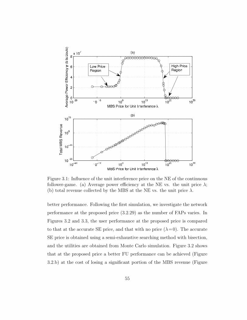
✶�✲✁✂
✶�✲✄✂
✶�✂
✶�✄✂
✶�✁✂
✶�✸✂
�
✷
✹
✻
✽① ✶�
✼
▼☎✆ ✝✞✟✠✡ ☛☞✞ ✌✍✟✎ ✏✍✎✡✞☛✡✞✡✍✠✡ ❧❆✑✒✓✔✕✒✖✗✘✒✓✙✚✚✛✜✛✒✢✜✣②
✥✤✛✦✧★✩✗✪✫✒✬
✭✮✯
✶�✲✁✂
✶�✲✄✂
✶�✂
✶�✄✂
✶�✁✂
✶�✸✂
✶�✲✁✂
✶�✲✄✂
✶�✂
✶�✄✂
▼☎✆ ✝✞✟✠✡ ☛☞✞ ✌✍✟✎ ✏✍✎✡✞☛✡✞✡✍✠✡ ❧
❚✗✦✔✫✰✱✳✴✒✑✒✢✪✒
✭✵✯
▲☞✺ ✝✞✟✠✡
❘✡✾✟☞✍
❍✟✾✿ ✝✞✟✠✡
❘✡✾✟☞✍
Figure 3.1: Influence of the unit interference price on the NE of the continuousfollower-game. (a) Average power efficiency at the NE vs. the unit price λ;(b) total revenue collected by the MBS at the NE vs. the unit price λ.
better performance. Following the first simulation, we investigate the network
performance at the proposed price (3.2.29) as the number of FAPs varies. In
Figures 3.2 and 3.3, the user performance at the proposed price is compared
to that at the accurate SE price, and that with no price (λ=0). The accurate
SE price is obtained using a semi-exhaustive searching method with bisection,
and the utilities are obtained from Monte Carlo simulation. Figure 3.2 shows
that at the proposed price a better FU performance can be achieved (Figure
3.2.b) at the cost of losing a significant portion of the MBS revenue (Figure
55
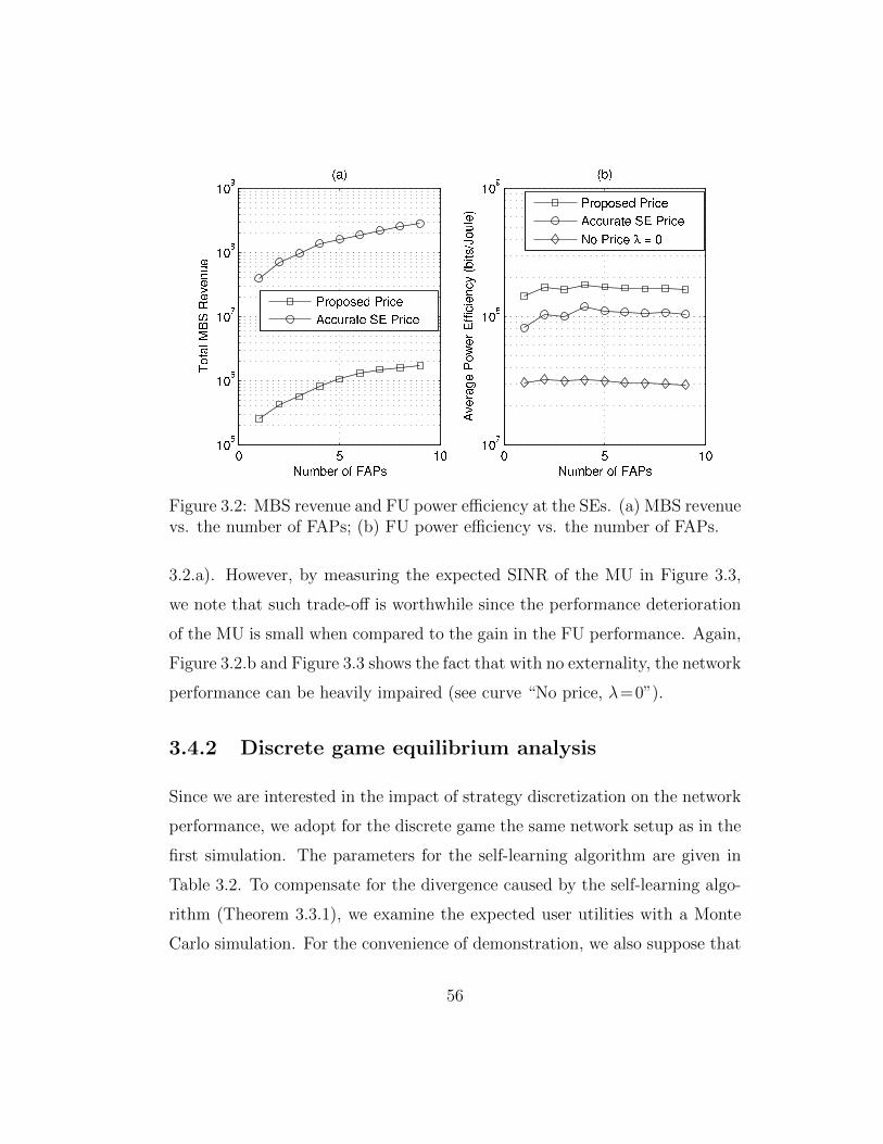
✵ ✺ ✶✵✶✵
�
✶✵✻
✶✵✼
✶✵✽
✶✵✾
◆✁✂✄☎✆ ✝✞ ✟✠✡☛
❚☞✌✍✎✏✑✒✓✔✕✔✖✗✔
✭✘✙
✡✆✝P✝☛☎✚ ✡✆✛✜☎
✠✜✜✁✆✘❆☎ ✢✣ ✡✆✛✜☎
✵ ✺ ✶✵✶✵
✼
✶✵✽
✶✵✾
◆✁✂✄☎✆ ✝✞ ✟✠✡☛
✤✕✔✥✍✦✔✧☞★✔✥✩✪✪✫✬✫✔✖✬✮✯✰✫✌✱✲✳☞✗✎✔✴
✭✄✙
✡✆✝P✝☛☎✚ ✡✆✛✜☎
✠✜✜✁✆✘❆☎ ✢✣ ✡✆✛✜☎
◆✝ ✡✆✛✜☎ ❧ ✷ ✵
Figure 3.2: MBS revenue and FU power efficiency at the SEs. (a) MBS revenuevs. the number of FAPs; (b) FU power efficiency vs. the number of FAPs.
3.2.a). However, by measuring the expected SINR of the MU in Figure 3.3,
we note that such trade-off is worthwhile since the performance deterioration
of the MU is small when compared to the gain in the FU performance. Again,
Figure 3.2.b and Figure 3.3 shows the fact that with no externality, the network
performance can be heavily impaired (see curve “No price, λ=0”).
3.4.2 Discrete game equilibrium analysis
Since we are interested in the impact of strategy discretization on the network
performance, we adopt for the discrete game the same network setup as in the
first simulation. The parameters for the self-learning algorithm are given in
Table 3.2. To compensate for the divergence caused by the self-learning algo-
rithm (Theorem 3.3.1), we examine the expected user utilities with a Monte
Carlo simulation. For the convenience of demonstration, we also suppose that
56
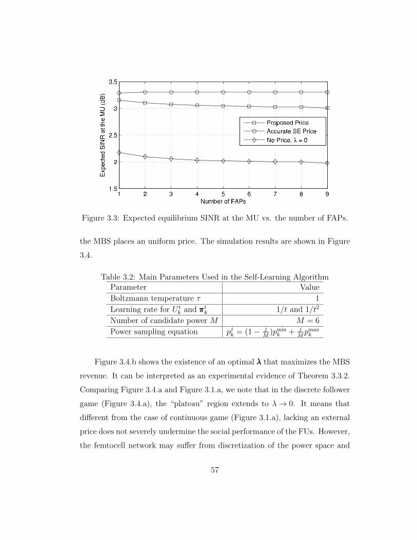
✶ ✷ ✸ ✹ ✺ ✻ ✼ ✽ ✾✶�✺
✷
✷�✺
✸
✸�✺
◆✁✂✄☎✆ ✝✞ ✟✠✡☛
❊☞✌✍✎✏✍✑✒✓✔✕
✖✏✏✗✍✘✙
✚✑✛✜
✡✆✝P✝☛☎✢ ✡✆✣✤☎
✠✤✤✁✆❆✥☎ ✦✧ ✡✆✣✤☎
◆✝ ✡✆✣✤☎★ ❧ ✩ ✪
Figure 3.3: Expected equilibrium SINR at the MU vs. the number of FAPs.
the MBS places an uniform price. The simulation results are shown in Figure
3.4.
Table 3.2: Main Parameters Used in the Self-Learning AlgorithmParameter Value
Boltzmann temperature τ 1
Learning rate for U tk and πππtk 1/t and 1/t2
Number of candidate power M M = 6
Power sampling equation pjk = (1− jM
)pmink + j
Mpmaxk
Figure 3.4.b shows the existence of an optimal λλλ that maximizes the MBS
revenue. It can be interpreted as an experimental evidence of Theorem 3.3.2.
Comparing Figure 3.4.a and Figure 3.1.a, we note that in the discrete follower
game (Figure 3.4.a), the “plateau” region extends to λ→ 0. It means that
different from the case of continuous game (Figure 3.1.a), lacking an external
price does not severely undermine the social performance of the FUs. However,
the femtocell network may suffer from discretization of the power space and
57
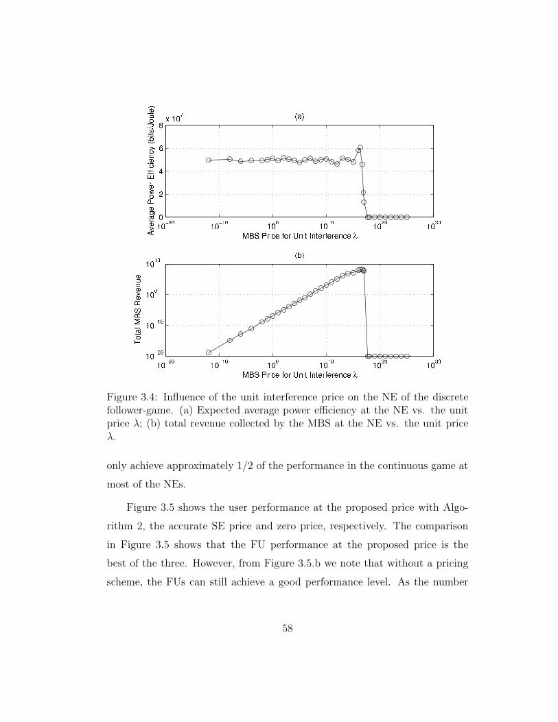
✶�✲✁✂
✶�✲✄✂
✶�✂
✶�✄✂
✶�✁✂
✶�✸✂
�
✷
✹
✻
✽① ✶�
✼
▼☎✆ ✝✞✟✠✡ ☛☞✞ ✌✍✟✎ ✏✍✎✡✞☛✡✞✡✍✠✡ ❧❆✑✒✓✔✕✒✖✗✘✒✓✙✚✚✛✜✛✒✢✜✣✤✥✛✦✧★✩✗✪✫✒✬
✭✮✯
✶�✲✁✂
✶�✲✄✂
✶�✂
✶�✄✂
✶�✁✂
✶�✸✂
✶�✲✁✂
✶�✲✄✂
✶�✂
✶�✄✂
▼☎✆ ✝✞✟✠✡ ☛☞✞ ✌✍✟✎ ✏✍✎✡✞☛✡✞✡✍✠✡ ❧
❚✗✦✔✫✰✱✳✴✒✑✒✢✪✒
✭✵✯
Figure 3.4: Influence of the unit interference price on the NE of the discretefollower-game. (a) Expected average power efficiency at the NE vs. the unitprice λ; (b) total revenue collected by the MBS at the NE vs. the unit priceλ.
only achieve approximately 1/2 of the performance in the continuous game at
most of the NEs.
Figure 3.5 shows the user performance at the proposed price with Algo-
rithm 2, the accurate SE price and zero price, respectively. The comparison
in Figure 3.5 shows that the FU performance at the proposed price is the
best of the three. However, from Figure 3.5.b we note that without a pricing
scheme, the FUs can still achieve a good performance level. As the number
58
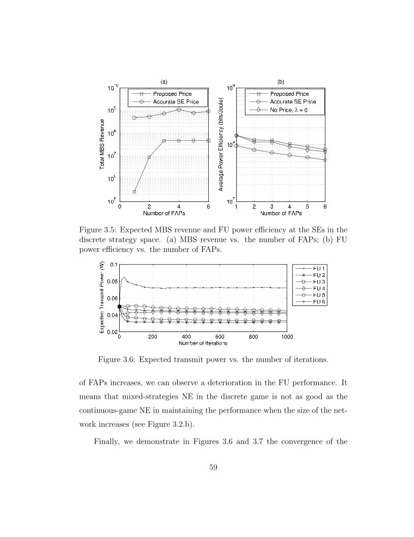
✵ ✷ ✹ ✻✶✵✺
✶✵�
✶✵✼
✶✵✽
✶✵✾
✶✵✁✂
◆✄☎✆✝✞ ✟✠ ✡☛☞✌
❚✍✎✏✑✒✓✔✕✖✗✖✘✙✖
✭✚✛
☞✞✟P✟✌✝✜ ☞✞✢✣✝
☛✣✣✄✞✚❆✝ ✤✥ ☞✞✢✣✝
✶ ✷ ✸ ✹ ✦ ✻✶✵✼
✶✵✽
✶✵✾
◆✄☎✆✝✞ ✟✠ ✡☛☞✌
✧✗✖★✏✩✖✪✍✫✖★✬✮✮✯✰✯✖✘✰✱✲✳✯✎✴✿❀✍✙✑✖❁
✭✆✛
☞✞✟P✟✌✝✜ ☞✞✢✣✝
☛✣✣✄✞✚❆✝ ✤✥ ☞✞✢✣✝
◆✟ ☞✞✢✣✝❂ ❧ ❃ ✵
Figure 3.5: Expected MBS revenue and FU power efficiency at the SEs in thediscrete strategy space. (a) MBS revenue vs. the number of FAPs; (b) FUpower efficiency vs. the number of FAPs.
✵ ✷✵✵ ✹✵✵ ✻✵✵ ✽✵✵ ✶✵✵✵✵�✵✷
✵�✵✹
✵�✵✻
✵�✵✽
✵�✶
◆✁✂✄☎✆ ✝✞ ✟✠☎✆✡✠☛✝☞✌
❊✍✎✏✑✒✏✓✔✕✖✗✘✙✚✒✛✜✢✏✕✣✤✥
❋✦ ✶
❋✦ ✷
❋✦ ✧
❋✦ ✹
❋✦ ★
❋✦ ✻
Figure 3.6: Expected transmit power vs. the number of iterations.
of FAPs increases, we can observe a deterioration in the FU performance. It
means that mixed-strategies NE in the discrete game is not as good as the
continuous-game NE in maintaining the performance when the size of the net-
work increases (see Figure 3.2.b).
Finally, we demonstrate in Figures 3.6 and 3.7 the convergence of the
59
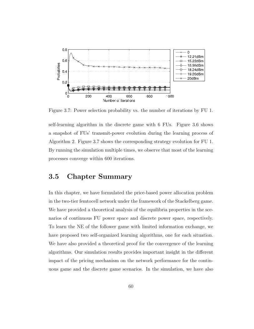
✵ ✷✵✵ ✹✵✵ ✻✵✵ ✽✵✵ ✶✵✵✵✵
✵�✷
✵�✹
✵�✻
✵�✽
◆✁✂✄☎✆ ✝✞ ✟✠☎✆✡✠☛✝☞✌
P✍✎✏✑✏✒✓✒✔✕
✵
✶✷�✷✶✖✗✂
✶✘�✷✷✖✗✂
✶✻�✙✙✖✗✂
✶✽�✷✹✖✗✂
✶✙�✷✵✖✗✂
✷✵✖✗✂
Figure 3.7: Power selection probability vs. the number of iterations by FU 1.
self-learning algorithm in the discrete game with 6 FUs. Figure 3.6 shows
a snapshot of FUs’ transmit-power evolution during the learning process of
Algorithm 2. Figure 3.7 shows the corresponding strategy evolution for FU 1.
By running the simulation multiple times, we observe that most of the learning
processes converge within 600 iterations.
3.5 Chapter Summary
In this chapter, we have formulated the price-based power allocation problem
in the two-tier femtocell network under the framework of the Stackelberg game.
We have provided a theoretical analysis of the equilibria properties in the sce-
narios of continuous FU power space and discrete power space, respectively.
To learn the NE of the follower game with limited information exchange, we
have proposed two self-organized learning algorithms, one for each situation.
We have also provided a theoretical proof for the convergence of the learning
algorithms. Our simulation results provides important insight in the different
impact of the pricing mechanism on the network performance for the contin-
uous game and the discrete game scenarios. In the simulation, we have also
60

shown the efficiency of the proposed heuristic price-searching mechanism in
the game. Our study provides an alternative way of designing the resource
allocation protocols since no inter-cell information exchange is required in the
femtocells.
61
Chapter 4
Learning for JointChannel-Power Allocation inSelf-Sustainable WirelessNetworks
Recent years has seen a surge in the energy consumption by cellular net-
works, which has already been considered a major source of the global CO2
emission. Specifically, Base Stations (BSs) and backhaul networks are respon-
sible for most of the energy consumption therein, with energy demand still
growing at a rate of 16-20% per year [51]. With the increasing concerns on
reducing CO2 emissions, significant efforts have been made toward designing
more environmentally friendly wireless networks. Across the substantial body
of research on improving energy efficiency in wireless networks ([51, 52] and
references therein), new techniques are proposed from both the BS perspective
(e.g., cell zooming and cooperative switching-off) and the end-device perspec-
tive (e.g., cooperative relaying and dynamic cell selection).
Apart from network-oriented approaches to green network design, recent
62
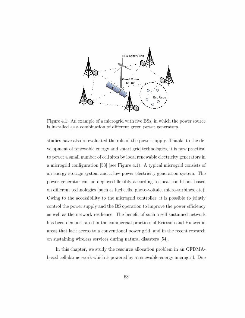
Figure 4.1: An example of a microgrid with five BSs, in which the power sourceis installed as a combination of different green power generators.
studies have also re-evaluated the role of the power supply. Thanks to the de-
velopment of renewable energy and smart grid technologies, it is now practical
to power a small number of cell sites by local renewable electricity generators in
a microgrid configuration [53] (see Figure 4.1). A typical microgrid consists of
an energy storage system and a low-power electricity generation system. The
power generator can be deployed flexibly according to local conditions based
on different technologies (such as fuel cells, photo-voltaic, micro-turbines, etc).
Owing to the accessibility to the microgrid controller, it is possible to jointly
control the power supply and the BS operation to improve the power efficiency
as well as the network resilience. The benefit of such a self-sustained network
has been demonstrated in the commercial practices of Ericsson and Huawei in
areas that lack access to a conventional power grid, and in the recent research
on sustaining wireless services during natural disasters [54].
In this chapter, we study the resource allocation problem in an OFDMA-
based cellular network which is powered by a renewable-energy microgrid. Due
63
to the power instability caused by the increased adoption of green sources, the
electric power system faces a conflict between the transmission-driven power
demand from the network and the limited power supply from the microgrid.
To establish a self-organized, sustainable resource management mechanism,
we model the joint power-transmission control in the network as a two-level
Stackelberg game [34]. On the cellular network level, we model the interaction
between the BSs and the mobile users as an auction-based follower game. In
order to solve for the subgame equilibrium, we propose a joint power-subcarrier
allocation algorithm in the form of iterative combinatorial auction [55]. On
the microgrid level, the power supply control is modeled as the leader game.
To improve the sustainability of the microgrid, we propose a pricing-based
method for the microgrid to adjust the power demand from the network level.
Theoretical analysis is provided to show the effectiveness of the proposed al-
gorithm.
4.1 System Model
We consider an OFDMA-based cellular network that is divided into a number
of “Sustainable Wireless Areas” (SWA). As demonstrated by Figure 4.1, each
SWA is composed of several BSs and self-organized as a stand-along microgrid.
The electric power in each microgrid is provided by an independent group
of renewable power generators. To manage the variability in the renewable
sources due to weather conditions, the renewable power is diversified by using
different sources (from wind turbines and solar panels in the present case). In
addition to the renewable energy source, the BS batteries are coordinated by
a Central Power Controller (CPC) to adjust the electricity output by storing
the energy surplus for later use.
64

4.1.1 Energy generation and consumption profile
We assume that the microgrid operates in a time-slotted manner. During one
time slot, the energy charge and depletion rates are assumed to be invariant2.
Then, the energy dynamic of a SWA can be described by the following linear
model:
Es(t+ 1) = Es(t) + αEc(t)− Ed(t), (4.1.1)
where Es(t), Ec(t) and Ed(t) are the total energy storage, the energy charge
and the energy depletion at time slot t, respectively. 0<α< 1 is a factor for
charge inefficiency.
We consider a hybrid energy source comprised by a photovotaic (PV) array
and a wind turbine. Based on the empirical studies of green power generation
[54,56], the variability of the output power can be modeled as Markov chains
by representing the operational state (see [56]) of the PV array and the wind
turbine with a number of discrete levels3. We denote the operational state of
the PV array and the wind turbine by ss∈Ss and sw∈Sw, respectively. Then,
we can express the energy charge as Ec(sts, s
tw) = T (ps(s
ts) + pw(stw)), where T
is the duration of time slot t, ps and pw are the output power of the PV array
and wind turbine in their respective states.
The energy consumption of a SWA, on the other hand, is determined by
the load of the BSs therein. According to [57], the power consumed by one
BS can be broken down into a power supply and maintenance component,
and a transmission service component. We consider a typical setup of mul-
tiple Macro/Micro BSs, and adopt a linear power consumption model [57] as
2In reality we work with the average value over the duration of each time slot.3The energy generation in the daytime and nighttime can be modeled by Markov chains
with different parameters.
65
Ekd = T (p0 + δppk(t)), where p0 is the minimum output power when no load
is serviced, δp is the slope of the load dependent power (i.e., the downlink
transmit power) and pk(t) is the transmit power in slot t.
4.1.2 Joint subcarrier-power allocation for mobilestations
We consider a generic scenario where a SWA contains K BSs and the total
bandwidth W is divided into N subcarriers. During time slot t, the BSs
receive the transmission request from M Mobile Stations (MSs). For each
BS, one subcarrier can be assigned to no more than one MS at the same time.
Meanwhile, each MS can only subscribe to a single BS during one time slot. We
assume that perfect instantaneous channel information is available at each BS,
and the intercell interference over each subcarrier is treated as noise4. Then,
for a MS m served by BS k over subcarrier n, the Signal-to-Interference-plus-
Noise-Ratio (SINR) can be written as follows (in what follows, we omit the
time slot indicator t for brevity):
βmkn = gmknpmkn/σ
2, (4.1.2)
where gmkn is the power gain, pmkn is the transmit power over the subcarrier, and
σ2 is the interference-plus-noise power. We assume Automatic Retransmis-
sion reQuest (ARQ) with perfect error detection. Then, adopting the effective
throughput model in [29], we can obtain the throughput achieved over a sub-
carrier as a function of the Bit-Error-Rate (BER):
rmkn(pmkn, cmkn) = ρR [1− pe(βmkn, cmkn)]B , (4.1.3)
4If a SWA is deployed as part of a large wireless network and both the MSs and BSs arerandomly distributed, the intercell interference to each MU can be treated as a standardM/M shot noise [58].
66
where ρ is the ratio of effective load to a packet length B, R is the transmit rate
over the subcarrier, and pe(βni , c
mkn) is the BER function, which is determined
by both the SNR βmkn and the code/modulation type cmkn [29].
From the perspective of a BS, it is natural to allocate the power and code
type over a subcarrier according to energy efficiency. Therefore, power and
code type allocation for a potential link from BS k to MS m over subcarrier n
can be pre-calculated as:
{(pmkn)∗, (cmkn)∗} = arg minpmkn,c
mkn
pmknrmkn(pmkn, c
mkn)
s.t. 0 < pmkn ≤ pkn, (4.1.4)
where pkn is the power limit over one subcarrier. Given the to-be-allocated
transmit parameters (pmkn)∗ and (cmkn)∗, the MSs evaluate the spectrum effi-
ciency of each subcarrier as
umkn = rmkn ((pmkn)∗, (cmkn)∗) . (4.1.5)
Considering the power and bandwidth budget for transmitting to one MS,
we limit the maximum number of subcarriers to be allocated to MS m as αm.
We also limit the minimum number of subcarriers to be allocated to MS m
as αm, which reflects the QoS requirement by each MS. By considering that
the BSs are able to work cooperatively, the resource allocation problem can
67
be formulated as
{dmkn} = arg max{dmkn}
M∑m=1
K∑k=1
N∑n=1
dmknumkn (4.1.6a)
s.t. αm ≤K∑k=1
N∑n=1
dmkn ≤ αm, ∀m (4.1.6b)
M∑m=1
dmkn ≤ 1, ∀k, ∀n (4.1.6c)
N∑n=1
dmkn
N∑n=1
dmjn=0, ∀k 6=j,∀m (4.1.6d)
M∑m=1
K∑k=1
N∑n=1
dmknpmkn ≤ p. (4.1.6e)
In (4.1.6a), dmkn∈{0, 1} is a binary variable that indicates if MS m chooses sub-
carrier n from BS k (dmkn=1) or not (dmkn=0); (4.1.6b) indicates the constraints
on the number of subcarriers that can be assigned to one MS; (4.1.6c) ensures
that for any BS, each subcarrier can only be assigned to one MS; (4.1.6d)
reflects the assumption that one MS can only choose a single BS for the trans-
mission during one time slot; (4.1.6e) is the power consumption constraint
and p is the upper limit on the supplied power. Problem (4.1.6a)-(4.1.6e) is
a binary programming problem with nonlinear constraints. It is similar to
a set-packing problem [55], which is known to be NP-complete. Due to the
excessive computational complexity and memory requirements, optimization-
based solutions such as branch-and-bound algorithm appear less attractive for
practical implementation. Moreover, it still remains an open issue to design
a power control mechanism that can balance between the variable power sup-
ply and the transmission demand by the network. Therefore, it is necessary
to design a resource allocation mechanism that is not only computationally
tractable, but also able to properly sustain the long term SWA operation.
68
4.2 Hierarchical formulation of resource
allocation
We assume that the CPC uses the energy price to control the power demand
and charges the network for what is consumed. The resource allocation pro-
cess within a SWA is modeled in two stages. In the first stage, the CPC
adjusts the power price according to its energy state and estimated future
power demand. In the second stage, the BSs and the MSs in the SWA jointly
determine the subcarrier-allocation scheme based on the network power pur-
chase budget. We note that the three parties, namely, the CPC, the BSs and
the MSs demonstrate conflicts in their private interest. In this sense, we can
again model the resource allocation process as a Stackelberg game [34]. In
the Stackelberg game framework, the CPC is modeled as the leader, while the
BSs and the MSs are modeled as the followers. With backward induction, we
start the system analysis by modeling the BS-MS interactions as a follower
subgame.
4.2.1 Subcarrier scheduling as combinatorial auction
We first focus on the BS-MS interaction and assume a fixed unit power price
λ. Based on (6), we model the joint power-subcarrier allocation process as an
auction game. Since the BSs work cooperatively, they can be considered as
a super auctioneer who owns multiple unique assets (i.e., K×N subcarriers)
for sale. Each MS is considered as a buyer who bids to get a certain subset
(package) of subcarriers from one BS. For the BSs, a virtual price qkn for
each subcarrier is introduced to help determine the package transactions. We
denote the set of all possible subcarrier packages by D = {D1, . . . ,D|D|}, in
69
which an element package Dj = [dj11, . . . , dj1N , d
j21, . . . , d
jKN ] should satisfy the
conditions (4.1.6b) and (4.1.6d) in order to be a feasible allocation. Note that
here we slightly abuse the notation djkn ∈ {0, 1} with j being the package ID.
By using D, we can replace the subcarrier-allocation indicator in problem (6)
with the packet assignment indicator, which is denoted as xmj∈{0, 1}. xmj =1
indicates that Dj is assigned to MS m. In the auction, the goal of the BSs
is to maximize the total revenue by selling subcarrier packages. Meanwhile,
each MS aims at purchasing the package that maximizes its own spectrum
efficiency.
In order to address the impact of the power price by the CPC, we modify
(4.1.5) and express each MU’s valuation for one subcarrier as umkn−λpmkn. Then,
the private valuation of package j by MU m can be expressed as:
vjm =∑
djkn∈Djdjkn (umkn − λpmkn) . (4.2.1)
For packageDj, the ask price by the BSs can be written as qj =∑
djkn∈Dj djknqkn.
Based on (4.2.1), MU m’s payoff can be expressed as πm(Dj,Q, λ) = vjm − qj,
where Q is the price set, Q 3 qj,∀j. We define the subcarrier-allocation
vector as X = [xmj : ∀m, j], then the BS revenue can be expressed as
Π(X,Q) =∑
m,j xmjqj. Observing the MS/BS payoff function and the alloca-
tion requirement, we note that the subcarrier auction game has the following
properties:
1) The auction is combinatorial, since a MS can submit a request for more
than one subcarrier (i.e., in a package).
2) The bidding language is XOR, for a MS can bid for multiple subcarrier
packages but win at most one of them.
70
3) The auction is of linear price according to (4.2.1), which means that a
package price is equal to the sum of the prices over all the items in that
package.
4) The price is anonymous, namely, for any MU m 6= j, the price of the
same package is the same.
According to the above properties, the subcarrier auction game falls into
the category of the combinatorial auction [55]. To study the relation between
the original resource allocation problem (6) and the auction game, we introduce
the concept of Competitive Equilibrium (CE) [59]:
Definition 4.2.1 (Competitive Equilibrium). In the combinatorial auction,
prices Q and allocations X∗ are in competitive equilibrium if
π∗m(Di:x∗mi=1,Q, λ) = maxDj∈D
(vjm − qj),∀m, (4.2.2)
Π(X∗,Q) = maxX∈X
∑xmj∈X
xmjqj, (4.2.3)
in which X is the set of all the feasible allocations.
If we ignore the power supply constraint (4.1.6e) for a moment and re-
place unkn in the objective function of (6) with the subcarrier evaluation in
(4.2.1), problem (6) would be equivalent to the efficient Combinatorial Allo-
cation Problem (CAP) [55] in the subcarrier auction. Based on the definition
of the private valuation and package assignment indicator, we can derive a
new optimization problem from (4.1.6a)-(4.1.6d) as the CAP in its standard
71
binary-linear-programming form [55]:
X∗ = arg max{xmj}
∑1≤m≤M
∑1≤j≤|D|
xmjvjm (4.2.4a)
s.t.∑
1≤j≤|D|
xmj ≤ 1, ∀m, (4.2.4b)
∑1≤j≤|D|
∑1≤m≤M
djknxmj ≤ 1, ∀n, k. (4.2.4c)
We note that (4.2.4b) guarantees that each MS can win no more than one allo-
cation, and it is similar to the constraint in (4.1.6d). (4.2.4c) guarantees that
the packages with overlapping items can never be assigned, and is equivalent
to the constraint in (4.1.6c). It is also worth of noting that the constraint in
(4.1.6b) (and partly in (4.1.6d)) has already been addressed when determining
the set of possible subcarrier packages D. The connection between the opti-
mization problem in (4.2.4a)-(4.2.4c) and the combinatorial auction game is
established by the following theorem:
Theorem 4.2.1 ([60]). The combinatorial subcarrier auction solves the effi-
cient CAP problem in (4.2.4a)-(4.2.4c) iff it realizes a set of CE prices and
an allocation that is supported in the CE.
4.3 Iterative Learning for Subcarrier
Allocation
4.3.1 Iterative auction mechanism for subcarrierallocation
Theorem 4.2.1 reveals that instead of directly solving the NP-complete CAP in
(4.2.4a)-(4.2.4c), we can obtain the efficient subcarrier allocation by looking for
72
a CE with a computationally tractable auction process. Thereby, we propose
an iterative subcarrier auction mechanism based on the auction design in [60]
where the bid-allocation choices are determined by an iterative, ascending
price-asking process. Briefly stated, the auction is in the form of a general
English auction and carried out in multiple rounds. In every round, the BSs
announce the ask price for each package and the new bids are collected from
the MSs. At the end of each round, a proper allocation is announced according
to the bids and the ask prices in this round. Based on the bidding result per
round, the prices of relevant packages will be increased in the next round, until
the state of the auction satisfies some termination condition.
We say that MS m adopts a Straightforward Bidding (SB) strategy when
its demand set is formed by the packages that myopically maximize its own
payoff πm. Given an ask price set Q, we define the ε-SB set of a MS as the
demand set that is within ε of maximizing its payoff based on the SB strategy:
εBm(Q)={Dj :πm(Dj,Q, λ)≥maxDi∈D
(vim−qi)−ε,Dj∈D}. (4.3.1)
In each round, the BSs need to determine the package allocation given the
demand set εBm of each MS. This is known as the Winner Determination
Problem (WDP) [55]. To formulate the WDP, we denote the bid price for
package Dj by MS m as bjm. Similarly to (4.2.4a)-(4.2.4c), the WDP can also
be formulated as a binary linear programming problem:
X∗ = arg max{xmj}
∑1≤m≤M
∑j:Dj∈εBm
xmjbjm (4.3.2a)
s.t.∑
j:Dj∈εBm
xmj ≤ 1, ∀m, (4.3.2b)
∑1≤m≤M
∑j:Dj∈εBm
djknxmj ≤ 1, ∀n, k. (4.3.2c)
73

Then in each round, the auctioneer only needs to solve the WDP according
to the submitted bids εBm, Although still being a NP-complete problem, the
new WDP in (12) is much smaller when compared with the original problem
in (4.2.4a)-(4.2.4c). When small enough, (12) can be directly solved by an
integer-programming based algorithm. Also, its solution can be approximately
obtained by algorithms that may be a greedy algorithm or a tree-search based
algorithm [61]. In this section, we adopt the greedy approximation in [61] to
solve the WDP.
After the WDP is formulated for each round, we are ready to define the
rules for updating the bidding prices and the ask prices. For the MSs, the
rules of bidding are set as follows:
1) For any MS to continue bidding for the same package, the bids must be
at least the same as the current ask price.
2) If a MS wins one allocation in the current round according to the solution
of the WDP (12), it must resubmit the bid for the same package in the
next round. However, the resubmitted bit for the allocated subcarrier
package from the previous round can be less than the ask price.
3) For any MS, a submitted bid that is less than the ask price will be its
final price, which means that it will not be able to improve the bidding
price for that package anymore.
We say that a bidder is unhappy if it does not receive any package allocation
in the current round. We define the rules for the ask price evolution as follows:
1) The ask price of package Dj is increased when at least one MS bidding
for Dj is unhappy. We denote the set of unhappy MSs byMu, then the
74

ask price is updated as:
qji+1 = max(qji , maxm∈Mu,Dj∈εBm
bjm + ε), (4.3.3)
where i is the index of the auction rounds.
2) The auction is terminated either when each of the MSs receives a package,
or when all the MSs submit the same bids in two consecutive rounds.
Formally, we present the iterative combinatorial subcarrier auction mechanism
in Table 4.1. Convergence of the iterative auction is guaranteed under the
proposed auction rules according to Theorem 4.3.1 [60]:
Theorem 4.3.1. The iterative subcarrier auction terminates in finite rounds
and is within a bound of 3εmin{K×N,M} of the optimal payoff by the solution
of the CAP in (4.2.4a)-(4.2.4c).
4.3.2 Power price adjustment for subcarrier demandcontrol
Observing (4.2.1)-(4.2.4a), we note that the subcarrier allocation X∗ is the
result of point-to-set mapping from R+ (λ ∈ R+) into the power set 2X , where
X is the set of all possible package allocations. Then it is natural to consider
that the objective of the CPC is to maximize its revenue:
λ∗=arg maxλ
W =λ∑
xmj(λ)∈X∗xmj(λ)
∑djkn∈Dj
djknpmkn
. (4.3.4)
Since the solution to (4.3.4) does not automatically prevent over-drain of en-
ergy, we also need to guarantee that the total allocated power is properly
75

Table 4.1: Iterative subcarrier auction mechanism
Initialization:
The BSs set up the package set D and the price increment step ε. TheMSs initialize their private valuation vjm based on the current power priceλ. The initial ask price is set to qji = 0.
Iterative Auction Round i:
1. The MSs submit their bids based on their myopic ε-SB set εBm, whichis obtained according to (4.3.1). The demand sets and the bid prices areadjusted according to the rules of bidding 1)-3).
2. The BSs generate the new allocation according to the solution of theWDP in (12) and announce it to the MSs.
3. The BSs check for the packages that are in the bid set of the unhappyMSs. The ask prices are updated according to (4.3.3).
4. The BSs check the termination condition according to the rule for theask price evolution 2). If it is not satisfied, the auction round index i isincremented, and a new auction round is started by looping to step 1.
limited. From the structure of (4.2.1) and (4.2.2), we note that λ is upper-
bounded. Otherwise, when λ is too large and makes λ > max(umkn/pmkn),∀k, n,m,
all the MSs will be forced to stop from requesting subcarriers. The reason is
straightforward: according to (4.2.2), for an individually rational MS, to stop
transmitting will result in a zero payoff, which will be the CE strategy when
the payoff in all the other cases is negative. Therefore, based on Theorems
4.2.1 and 4.3.1, we have the following proposition:
Proposition 4.3.1. With the proposed auction mechanism, a power price λ
can always be found to satisfy the power constraint:∑xmj(λ)∈X∗
xmj(λ)∑
djkn∈Dj
djknpmkn ≤ pT , (4.3.5)
where X∗ is the subcarrier allocation by the auction and pT > 0 is a power
76

Table 4.2: Bisection Based Power Price Updating
Initialization:
Obtain the power threshold pT according to (4.3.6). Set the lower priceas λl = 0 and the upper price as λu = 2 max(umkn/p
mkn), ∀k, n,m. Initialize
the CPC revenue record as W = 0.
Repeat:
1. Set λt = (λl + λu)/2.
2. Run the iterative auction algorithm according to Table 4.1 to obtainthe power and subcarrier allocation.
3. Check the feasibility of (4.3.5). If (4.3.5) is feasible, set λu ← λt,otherwise set λl ← λt.
4. If (4.3.5) is feasible, calculate the CPC revenueWt according to (4.3.4).If Wt > W , set W ← Wt.
5. If Wt < W or |λt − λt−1| < θ, exit the loop.
threshold.
With Proposition 4.3.1, we are now ready to determine the power con-
sumption constraint for (4.3.4). We consider that the SWA is required to
maintain its energy storage above a critical level, which is given by Es(t).
Then based on (4.1.1) and the model of BS power consumption in Section
II-A, we can obtain the threshold for time slot t as follows:
pT (t) =1
δpT
(Es(t− 1) + αEc(t)− Es(t)−Kp0T
). (4.3.6)
We consider that Es(t) is a pre-known value and is determined by the expected
energy storage in different charge states.
It is difficult to find the exact Stackelberg equilibrium of the auction based
resource allocation process, namely, the set Q, X∗ and the price λ∗ that solve
(4.3.4) and satisfy (4.2.2) and (4.2.3) at the same time. However, it is possible
77
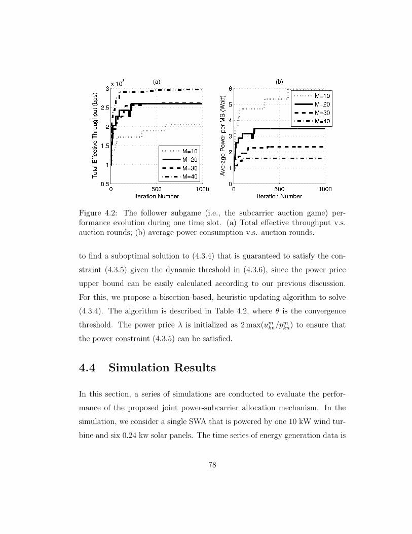
✵ ✺✵✵ ✶✵✵✵✵�✺
✶
✶�✺
✷
✷�✺
✸① ✶✵
✻
■✁✂✄☎✁✆✝✞ ✟✠✡☛✂✄
❚☞✌✍✎✏✑✑✒✓✌✔✕✒❚✖✗☞✘✙✖✚✘✌✛✜✚✢✣
✭☎✤
✵ ✺✵✵ ✶✵✵✵✵
✶
✷
✸
✹
✺
✥
■✁✂✄☎✁✆✝✞ ✟✠✡☛✂✄
❆✕✒✗✍✙✒✦☞✧✒✗✚✒✗★✩✛✪✍✌✌✣
✭☛✤
▼✫✶✵
▼✫✷✵
▼✫✸✵
▼✫✹✵
▼✫✶✵
▼✫✷✵
▼✫✸✵
▼✫✹✵
Figure 4.2: The follower subgame (i.e., the subcarrier auction game) per-formance evolution during one time slot. (a) Total effective throughput v.s.auction rounds; (b) average power consumption v.s. auction rounds.
to find a suboptimal solution to (4.3.4) that is guaranteed to satisfy the con-
straint (4.3.5) given the dynamic threshold in (4.3.6), since the power price
upper bound can be easily calculated according to our previous discussion.
For this, we propose a bisection-based, heuristic updating algorithm to solve
(4.3.4). The algorithm is described in Table 4.2, where θ is the convergence
threshold. The power price λ is initialized as 2 max(umkn/pmkn) to ensure that
the power constraint (4.3.5) can be satisfied.
4.4 Simulation Results
In this section, a series of simulations are conducted to evaluate the perfor-
mance of the proposed joint power-subcarrier allocation mechanism. In the
simulation, we consider a single SWA that is powered by one 10 kW wind tur-
bine and six 0.24 kw solar panels. The time series of energy generation data is
78
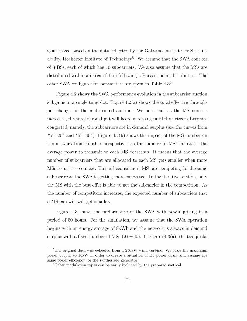
synthesized based on the data collected by the Golisano Institute for Sustain-
ability, Rochester Institute of Technology5. We assume that the SWA consists
of 3 BSs, each of which has 16 subcarriers. We also assume that the MSs are
distributed within an area of 1km following a Poisson point distribution. The
other SWA configuration parameters are given in Table 4.36.
Figure 4.2 shows the SWA performance evolution in the subcarrier auction
subgame in a single time slot. Figure 4.2(a) shows the total effective through-
put changes in the multi-round auction. We note that as the MS number
increases, the total throughput will keep increasing until the network becomes
congested, namely, the subcarriers are in demand surplus (see the curves from
“M=20” and “M=30”). Figure 4.2(b) shows the impact of the MS number on
the network from another perspective: as the number of MSs increases, the
average power to transmit to each MS decreases. It means that the average
number of subcarriers that are allocated to each MS gets smaller when more
MSs request to connect. This is because more MSs are competing for the same
subcarrier as the SWA is getting more congested. In the iterative auction, only
the MS with the best offer is able to get the subcarrier in the competition. As
the number of competitors increases, the expected number of subcarriers that
a MS can win will get smaller.
Figure 4.3 shows the performance of the SWA with power pricing in a
period of 50 hours. For the simulation, we assume that the SWA operation
begins with an energy storage of 8kWh and the network is always in demand
surplus with a fixed number of MSs (M=40). In Figure 4.3(a), the two peaks
5The original data was collected from a 250kW wind turbine. We scale the maximumpower output to 10kW in order to create a situation of BS power drain and assume thesame power efficiency for the synthesized generator.
6Other modulation types can be easily included by the proposed method.
79
Table 4.3: SWA Configuration Parameters for the SimulationParameter Value
Price increment step ε 1bps
Maximum power per subcarrier pkn 33dBm
Limits of subcarrier allocation [α, α] [2, 4]
Modulation types non-coherent FSK, DPSK
Interference plus noise power −30dBm
Transmit rate R over each subcarrier 0.1Mbps
Minimum operation power p0 504W (see [57])
Load dependent power slope δp 16.8 (see [57])
of the generated power at hour 16 and hour 39 represent the daytime hours. We
can observe from Figure 4.3(b) that until hour 40, the allocation mechanism
is able to sustain the network operation with the help of the BS batteries and
distribute the power as much as possible. However, in a bad weather condition
(e.g., after hour 41), the SWA still faces the danger of energy depletion and
needs the power from a conventional grid if it wants to provide a service that
supports any transmission (see the sub-figure in Figure 4.3(a)).
We finally compare the proposed algorithm with conventional allocation
methods based on random allocation and on a suboptimal adaptive allocation
algorithm. The random allocation algorithm (curve “Random” in Figure 4.4)
randomly assigns a BS and its subcarriers to each MS. The suboptimal adap-
tive allocation algorithm (curve “Adaptive” in Figure 4.4) applies a greedy
allocation method, which is a variation of the two-stage BS-subcarrier alloca-
tion method proposed in [62] based on the problem formulation in subproblem
(4.1.6). Figure 4.4(a) shows the performance of the three algorithms based on
the assumption that the power supply is always sufficient. From Figure 4.4(a)
we can observe that the proposed algorithm is able to improve the network
80
✵ ✺ ✶✵ ✶✺ ✷✵ ✷✺ ✸✵ ✸✺ ✹✵ ✹✺ ✺✵✵
✷✵✵✵
✹✵✵✵
✻✵✵✵
✽✵✵✵
❖�✁✂✄☎✆✝✞✄✟ ✠✝✡✂
P☛☞✌✍✎✏✑✒✒✓
✭✄✔
●✁✞✁✂✄☎✁✕ ✖✝✗✁✂
❈✝✞✘✡✙✁✕ ✖✝✗✁✂
✵ ✺ ✶✵ ✶✺ ✷✵ ✷✺ ✸✵ ✸✺ ✹✵ ✹✺ ✺✵✵
✶
✷
✸
✹① ✶✵
✚
❖�✁✂✄☎✆✝✞✄✟ ✠✝✡✂
❚☛✒✑✛❚✜✍☛✢✣✜✤✢✒✎✥✤✦✓
✭✧✔
✵ ✷✵ ✹✵✵
✺
✶✵① ✶✵
✼
❖�✁✂✄☎✆✝✞✄✟ ✠✝✡✂❙✒☛✍✑✣✌✌✎★☛✢✛✌✓
Figure 4.3: Performance evolution with power pricing. (a) Power consump-tion/generation v.s. time; (b) total throughput v.s. time.
performance in terms of expected total throughput by 50%. In Figure 4.4(b),
we measure the percentage of the system’s operational time (whenever the BSs
are able to support transmission) with the three algorithms. The same power
generation series is assumed. From 4.4(b), we can observe that the proposed
algorithm is able to improve the percentage of operational time by 30% than
the algorithms without power pricing.
81
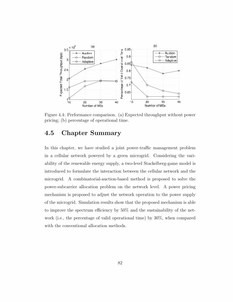
✶� ✷� ✸� ✹�✶
✶✁✂
✷
✷✁✂
✸
✸✁✂① ✶�
✻
◆✄☎✆✝✞ ✟✠ ✡☛☞
❊✌✍✎✏✑✎✒✓✔✑✕✖✓✗✘✔✙✚✗✍✙✑✛✜✍✢✣
✭✤✥
❆✄✦✧★✟✩
❘✤✩✪✟☎
❆✪✤✫✧★✬✝
✶� ✷� ✸� ✹�
�✁✵✂
�✁✮
�✁✮✂
�✁✯
�✁✯✂
�✁✰
�✁✰✂
◆✄☎✆✝✞ ✟✠ ✡☛☞
P✎✘✏✎✱✑✕✚✎✔✲✳✕✖✴✒✺✍✎✘✕✑✴✔✱✕✖✓✴✼✎
✭✆✥
❆✄✦✧★✟✩
❘✤✩✪✟☎
❆✪✤✫✧★✬✝
Figure 4.4: Performance comparison. (a) Expected throughput without powerpricing; (b) percentage of operational time.
4.5 Chapter Summary
In this chapter, we have studied a joint power-traffic management problem
in a cellular network powered by a green microgrid. Considering the vari-
ability of the renewable energy supply, a two-level Stackelberg-game model is
introduced to formulate the interaction between the cellular network and the
microgrid. A combinatorial-auction-based method is proposed to solve the
power-subcarrier allocation problem on the network level. A power pricing
mechanism is proposed to adjust the network operation to the power supply
of the microgrid. Simulation results show that the proposed mechanism is able
to improve the spectrum efficiency by 50% and the sustainability of the net-
work (i.e., the percentage of valid operational time) by 30%, when compared
with the conventional allocation methods.
82
Chapter 5
Learning for Robust RoutingBased on Stochastic Game inCognitive Radio Networks
DSA-based CRNs require Secondary Users (SUs) to opportunistically ac-
cess idle channels which are temporarily unused by the Primary Users (PUs).
Although being considered an efficient way of spectrum utilization [7], DSA
results in a lack of static channels for SUs. As a result, new coupling between
the PHY-MAC layers and upper layer protocols arises. At the network layer,
a routing protocol is thus expected to explicitly address the impact of unstable
channels on the topology and the link performance of the secondary network.
Generally, routing problems in CRNs exhibit a certain level of similarity to
routing problems in multi-channel ad hoc networks [63]. However, routing in
CRNs faces a number of new, different challenges [63,64]:
(i) spectrum awareness: timely adaptation to the channel availability dy-
namic change due to DSA, and
83
(ii) self-organization: proper route configuration with limited/heterogeneous
channel resource knowledge.
Due to information uncertainty or locality associated with DSA, a dis-
tributed route discovery process in CRNs also tends to be more vulnerable to
insider attacks than in conventional ad-hoc networks. As indicated in [65,66],
an attacker in CRNs exploits the following characteristics of DSA schemes: (i)
vulnerabilities due to information locality with respect to spectrum state sens-
ing and reporting, and (ii) imperfect knowledge of SUs about the time-varying
PU channels. Since the channel state information accuracy directly affects the
performance of the DSA schemes in CRNs, most of the identified attacks in
CRNs target the distortion of channel state information to attack the PHY
and MAC protocols [67–69]. Similarly, it is now possible for routing attackers
to bypass the network-layer vulnerabilities used by traditional routing attack
schemes and only need to distort the channel detection/access information in
the DSA mechanism to disrupt the routing process.
In this chapter, we study a routing mechanism in a multi-hop, multi-
channel CRN and address the challenges of spectrum awareness, information
locality and routing security as an integrated problem. We consider limited
spectrum sensing abilities for each SU in a real-world situation. We also con-
sider the presence of malicious SUs which can apply sophisticated attacks by
combining different methods of attacks including Sink-Hole (SH) and Routing-
toward-Primary-User (RPU). In order to tackle the routing-under-attack prob-
lem for multiple flows, we formulate the joint channel-relay selection process
at the SUs as a stochastic game. We propose a distributed, adaptive channel-
relay selection scheme for SUs to learn their routing strategies with only limited
amount of information exchange. To defend the SH attack with information
84
distortion, we model the routing performance evaluation process as a Multi-
Arm Bandit (MAB) problem and use the estimated arm-selection probability
as an indicator of the neighbor trustworthiness. The proposed routing scheme
becomes a self-organized strategy-learning process in a series of single-state
repeated games. Neither the a-priori channel activity model nor information
flooding among the SUs is required for implementing the learning scheme.
5.1 Challenges in Designing a Robust
Routing Mechanism for CRNs
5.1.1 Routing in CRNs
The solutions to the routing problems in CRNs are usually characterized by a
cross-layer design that directly integrates channel sensing and MAC operations
into the routing protocols. These routing protocols may vary significantly
due to different assumptions on the PU activity model and DSA mechanisms.
Such variation is usually reflected by differences in the selection of link metrics
and routing scheme types (e.g., reactive and proactive). With respect to the
different channel occupation models (e.g., underlay vs. overlay/interweaving),
the link metrics may be designed in different ways. For overlay/interweaving
CRNs, many studies designed the routing mechanism based on a snapshot
of the channel dynamics [70–74]. In these studies, delay-based link quality
metrics were proposed based on a collision map for the SUs over the PU
channels. For underlay CRNs, the link quality metric may be designed based
on the link capacity as a function of the interference to the PUs [75]. For
both groups of solutions, routing schemes were usually designed in a time-
slotted manner to analyze and optimize the impact of DSA mechanisms on the
85
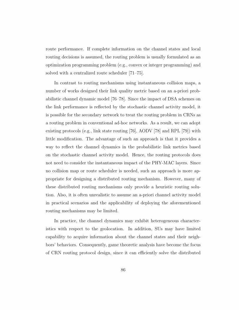
route performance. If complete information on the channel states and local
routing decisions is assumed, the routing problem is usually formulated as an
optimization programming problem (e.g., convex or integer programming) and
solved with a centralized route scheduler [71–75].
In contrast to routing mechanisms using instantaneous collision maps, a
number of works designed their link quality metric based on an a-priori prob-
abilistic channel dynamic model [76–78]. Since the impact of DSA schemes on
the link performance is reflected by the stochastic channel activity model, it
is possible for the secondary network to treat the routing problem in CRNs as
a routing problem in conventional ad-hoc networks. As a result, we can adopt
existing protocols (e.g., link state routing [76], AODV [78] and RPL [79]) with
little modification. The advantage of such an approach is that it provides a
way to reflect the channel dynamics in the probabilistic link metrics based
on the stochastic channel activity model. Hence, the routing protocols does
not need to consider the instantaneous impact of the PHY-MAC layers. Since
no collision map or route scheduler is needed, such an approach is more ap-
propriate for designing a distributed routing mechanism. However, many of
these distributed routing mechanisms only provide a heuristic routing solu-
tion. Also, it is often unrealistic to assume an a-priori channel activity model
in practical scenarios and the applicability of deploying the aforementioned
routing mechanisms may be limited.
In practice, the channel dynamics may exhibit heterogeneous character-
istics with respect to the geolocation. In addition, SUs may have limited
capability to acquire information about the channel states and their neigh-
bors’ behaviors. Consequently, game theoretic analysis have become the focus
of CRN routing protocol design, since it can efficiently solve the distributed
86
control problems with information exchange constraints. Game-based routing
solutions can be found in the studies on spectrum-aware, multi-flow rout-
ing [80,81] and traffic engineering [82] in CRNs. In these studies, the SUs are
assumed to be non-malicious and honest in sharing information, and the re-
peated (noncooperative) game models are usually applied. Cooperation among
SUs is implicitly enforced through repeatedly playing the game and the per-
formance of a route is ensured by the value of the game.
5.1.2 Security issues for routing in CRNs
In the literature, most of the studies on security problems in routing protocols
address conventional ad-hoc networks [83,84]. In these studies, the main focus
is to prevent information distortion (e.g., with public-key distribution [85]) or
to identify the attackers with limited traffic monitoring (e.g., [86, 87]). When
game theoretic solutions are adopted, the interaction between the honest and
malicious nodes is typically modeled as a constant/zero-sum game and solved
by obtaining the minimax equilibrium strategies in the game (e.g., [88, 89]).
There are relatively few works on secured routing protocol design in CRNs.
Among them, most of the studies are confined to handling the jamming at-
tacks or PUE attacks which distort the quality of an established link between
legitimated (normal) SUs (e.g., [90]). A more sophisticated routing attacks in
CRNs recently identified is the Routing-toward-Primary-User (RPU) attack
in multi-hop, overlay CRNs [91]. Unlike the PHY-MAC-layer focused attacks,
the RPU attack exploits the geographical heterogeneity in PU activities and
tunnels the traffic to the SUs that are in the footprint of the PU transmission.
An RPU attacker emulates a combined attacking mechanism of both the Sink-
Hole (SH) attack [83] and the Selective-Forwarding (SF) attack [83]. However,
87
the RPU-caused packet drop/delay is not due to the network layer operation
directly, but due to the collisions with PU transmissions on the PHY-MAC
layers.
5.2 Network Model and Link Metric
We consider a multi-hop CRN that interweaves upon K orthogonal PU chan-
nels. Normal SUs abide by the interweaving DSA rule and establish links over
the PU channels that are temporarily free. The nodes in the CRN are divided
into three types: the source SUs, sink SUs and relay SUs. We consider that
the relay SUs do not generate packets and only forward received packets to
their neighbors. Among the relay SUs, some malicious nodes adopt RPU-like
attacks to add delay to the traffic as much as possible.
5.2.1 Dynamic spectrum access model
Based on the empirical study of the PU channel occupation time in [92], we
assume that the PU activities over each channel can be modeled as an in-
dependent continuous-time Markov process with binary states Idle (‘0’) and
Busy (‘1’). For a channel k, we assume that λ−1k and µ−1k are the mean hold-
ing time for states Idle and Busy, respectively. Then, the corresponding state
transition matrix is given by [92]
Pk(t)=1
λk+µk
(µk+λke
−(λk+µk)t λk − λke−(λk+µk)tµk−µke−(λk+µk)t λk+µke
−(λk+µk)t
). (5.2.1)
Since in practical scenarios the PU activities are usually geographically dif-
ferent, we assume that the CRN can be geographically divided into a set of
88
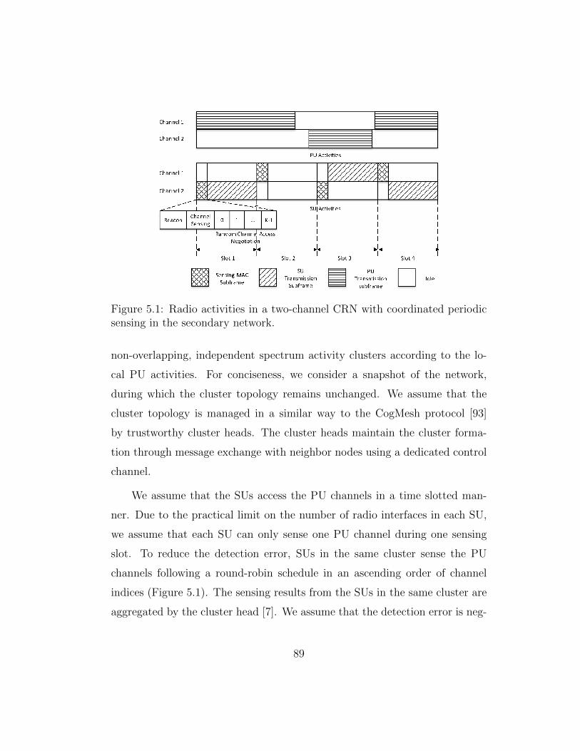
Figure 5.1: Radio activities in a two-channel CRN with coordinated periodicsensing in the secondary network.
non-overlapping, independent spectrum activity clusters according to the lo-
cal PU activities. For conciseness, we consider a snapshot of the network,
during which the cluster topology remains unchanged. We assume that the
cluster topology is managed in a similar way to the CogMesh protocol [93]
by trustworthy cluster heads. The cluster heads maintain the cluster forma-
tion through message exchange with neighbor nodes using a dedicated control
channel.
We assume that the SUs access the PU channels in a time slotted man-
ner. Due to the practical limit on the number of radio interfaces in each SU,
we assume that each SU can only sense one PU channel during one sensing
slot. To reduce the detection error, SUs in the same cluster sense the PU
channels following a round-robin schedule in an ascending order of channel
indices (Figure 5.1). The sensing results from the SUs in the same cluster are
aggregated by the cluster head [7]. We assume that the detection error is neg-
89
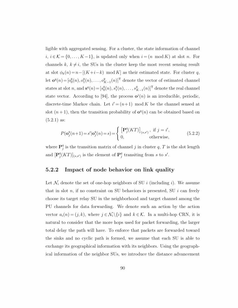
ligible with aggregated sensing. For a cluster, the state information of channel
i, i∈K= {0, . . . , K−1}, is updated only when i= (n modK) at slot n. For
channels k, k 6= i, the SUs in the cluster keep the most recent sensing result
at slot φk(n)=n−[(K+i−k) modK] as their estimated state. For cluster q,
let oq(n)=[oq0(n), oq1(n), . . . , oqK−1(n)]T denote the vector of estimated channel
states at slot n, and sq(n)=[sq0(n), sq1(n), . . . , sqK−1(n)]T denote the real channel
state vector. According to [94], the process oj(n) is an irreducible, periodic,
discrete-time Markov chain. Let i′= (n+1) modK be the channel sensed at
slot (n+ 1), then the transition probability of oq(n) can be obtained based on
(5.2.1) as:
P (oqj(n+1)=s′|oqj(n)=s)=
{ [Pqj(KT )
](s,s′)
, if j = i′,
0, otherwise,(5.2.2)
where Pqj is the transition matrix of channel j in cluster q, T is the slot length
and [Pqj(KT )](s,s′) is the element of Pq
j transiting from s to s′.
5.2.2 Impact of node behavior on link quality
Let Ni denote the set of one-hop neighbors of SU i (including i). We assume
that in slot n, if no constraint on SU behaviors is presented, SU i can freely
choose its target relay SU in the neighborhood and target channel among the
PU channels for data forwarding. We denote such an action by the action
vector ai(n) = (j, k), where j ∈Ni\{i} and k ∈K. In a multi-hop CRN, it is
natural to consider that the more hops used for packet forwarding, the larger
total delay the path will have. To enforce that packets are forwarded toward
the sinks and no cyclic path is formed, we assume that each SU is able to
exchange its geographical information with its neighbors. Using the geograph-
ical information of the neighbor SUs, we introduce the distance advancement
90
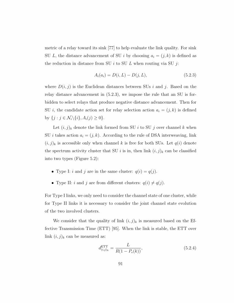
metric of a relay toward its sink [77] to help evaluate the link quality. For sink
SU L, the distance advancement of SU i by choosing ai = (j, k) is defined as
the reduction in distance from SU i to SU L when routing via SU j:
Ai(ai) = D(i, L)−D(j, L), (5.2.3)
where D(i, j) is the Euclidean distances between SUs i and j. Based on the
relay distance advancement in (5.2.3), we impose the rule that an SU is for-
bidden to select relays that produce negative distance advancement. Then for
SU i, the candidate action set for relay selection action ai = (j, k) is defined
by {j : j ∈ Ni\{i}, Ai(j) ≥ 0}.
Let (i, j)k denote the link formed from SU i to SU j over channel k when
SU i takes action ai = (j, k). According to the rule of DSA interweaving, link
(i, j)k is accessible only when channel k is free for both SUs. Let q(i) denote
the spectrum activity cluster that SU i is in, then link (i, j)k can be classified
into two types (Figure 5.2):
• Type I: i and j are in the same cluster: q(i) = q(j).
• Type II: i and j are from different clusters: q(i) 6= q(j).
For Type I links, we only need to consider the channel state of one cluster, while
for Type II links it is necessary to consider the joint channel state evolution
of the two involved clusters.
We consider that the quality of link (i, j)k is measured based on the Ef-
fective Transmission Time (ETT) [95]. When the link is stable, the ETT over
link (i, j)k can be measured as:
dETT(i,j)k
=L
R(1− Pe(k)), (5.2.4)
91
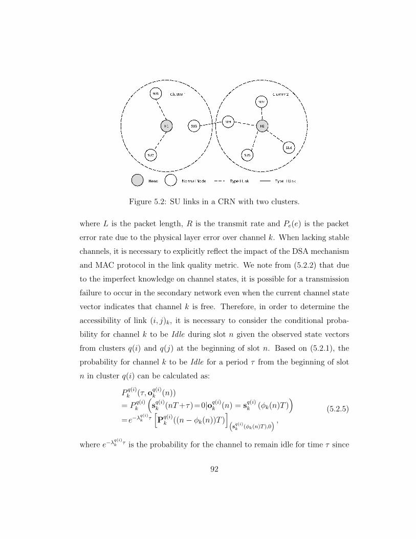
Figure 5.2: SU links in a CRN with two clusters.
where L is the packet length, R is the transmit rate and Pe(e) is the packet
error rate due to the physical layer error over channel k. When lacking stable
channels, it is necessary to explicitly reflect the impact of the DSA mechanism
and MAC protocol in the link quality metric. We note from (5.2.2) that due
to the imperfect knowledge on channel states, it is possible for a transmission
failure to occur in the secondary network even when the current channel state
vector indicates that channel k is free. Therefore, in order to determine the
accessibility of link (i, j)k, it is necessary to consider the conditional proba-
bility for channel k to be Idle during slot n given the observed state vectors
from clusters q(i) and q(j) at the beginning of slot n. Based on (5.2.1), the
probability for channel k to be Idle for a period τ from the beginning of slot
n in cluster q(i) can be calculated as:
Pq(i)k (τ,o
q(i)k (n))
= Pq(i)k
(sq(i)k (nT+τ)=0|oq(i)k (n) = s
q(i)k (φk(n)T )
)=e−λ
q(i)k τ
[Pq(i)k ((n− φk(n))T )
](sq(i)k (φk(n)T ),0
) ,(5.2.5)
where e−λq(i)k τ is the probability for the channel to remain idle for time τ since
92
the beginning of slot n, and[Pq(i)k ((n− φk(n))T )
](sq(i)k (φk(n)T ),0
) is obtained
from (5.2.1).
The availability probability for link (i, j)k at slot n depends on the prob-
ability of channel k staying idle at both end SUs. Based on our discussion of
the link type, the probability of channel k being available for link (i, j)k during
slot n can be expressed as:
P i,jk (o(n))=P i,j
k (oq(i)k (n),o
q(j)k (n)) ={
Pq(i)k (T,o
q(i)k (n)), if q(i)=q(j),
Pq(i)k (T,o
q(i)k (n))P
q(j)k (T,o
q(j)k (n)), if q(i) 6=q(j),
(5.2.6)
where o is the concatenation of the observed state vectors from all the clusters.
Based on (5.2.4) and (5.2.6), we can obtain the spectrum-aware link delay
metric for (i, j)k at slot n as follows:
d(i,j)k(o(n))=T(
1−P i,jk (o
q(i)k (n),o
q(j)k (n))
)+ dETT
(i,j)kP i,jk (o
q(i)k (n),o
q(j)k (n)),
(5.2.7)
where o(n) represents the joint state of the entire secondary network at time
slot n.
Now we consider the impact of the MAC protocol on the state of link
availability. Let Ai=Ni\{i}×K denote the set of candidate actions for SU i.
Due to the channel instability, it is difficult to directly adopt MAC protocols
based on single-channel random access with exponential backoff in the sec-
ondary network. Instead, we consider that the contention over each channel is
resolved through a reservation mechanism over the common control channel.
We consider that the negotiating phase over the control channel is divided into
K subslots, and the SUs compete for channel k in the corresponding subslot
by sending Request-To-Send (RTS) packets and listening to Clear-To-Send
93
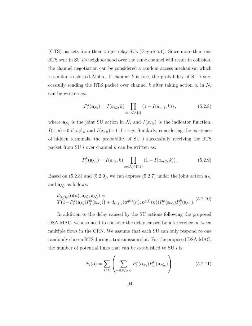
(CTS) packets from their target relay SUs (Figure 5.1). Since more than one
RTS sent in SU i’s neighborhood over the same channel will result in collision,
the channel negotiation can be considered a random access mechanism which
is similar to slotted-Aloha. If channel k is free, the probability of SU i suc-
cessfully sending the RTS packet over channel k after taking action ai in Nican be written as:
P ki (aNi
) = I(ai,2, k)∏
m∈Ni\{i}
(1− I(am,2, k)) , (5.2.8)
where aNiis the joint SU action in Ni and I(x, y) is the indicator function.
I(x, y)=0 if x 6=y and I(x, y)=1 if x=y. Similarly, considering the existence
of hidden terminals, the probability of SU j successfully receiving the RTS
packet from SU i over channel k can be written as:
P kj (aNj
) = I(ai,2, k)∏
m∈Nj\{i,j}
(1− I(am,2, k)) . (5.2.9)
Based on (5.2.8) and (5.2.9), we can express (5.2.7) under the joint action aNi
and aNjas follows:
d(i,j)k(o(n), aNi, aNj
) =
T(1−P k
i (aNi)P k
j (aNj))
+ d(i,j)k(oq(i)(n),oq(j)(n))P ki (aNi
)P kj (aNj
).(5.2.10)
In addition to the delay caused by the SU actions following the proposed
DSA-MAC, we also need to consider the delay caused by interference between
multiple flows in the CRN. We assume that each SU can only respond to one
randomly chosen RTS during a transmission slot. For the proposed DSA-MAC,
the number of potential links that can be established to SU i is:
Ni(a) =∑k∈K
∑m∈Ni\{i}
P ki (aNi
)P km(aNm)
, (5.2.11)
94
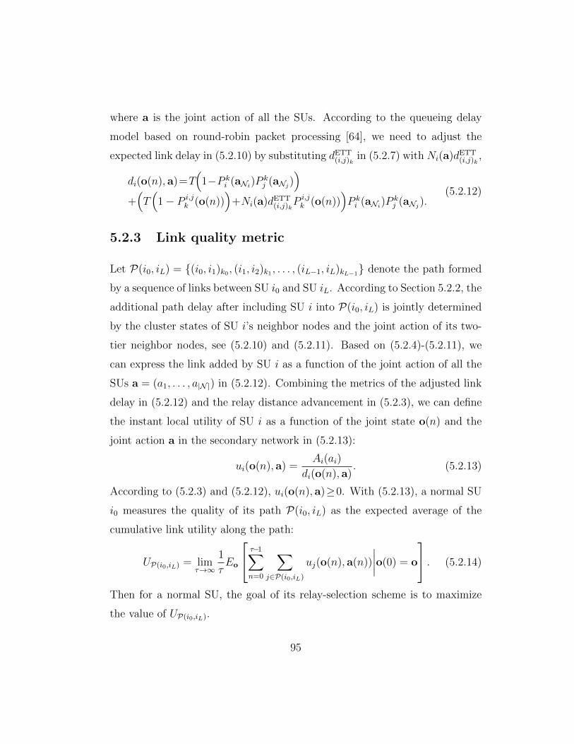
where a is the joint action of all the SUs. According to the queueing delay
model based on round-robin packet processing [64], we need to adjust the
expected link delay in (5.2.10) by substituting dETT(i,j)k
in (5.2.7) with Ni(a)dETT(i,j)k
,
di(o(n), a)=T(
1−P ki (aNi
)P kj (aNj
))
+(T(
1− P i,jk (o(n))
)+Ni(a)dETT
(i,j)kP i,jk (o(n))
)P ki (aNi
)P kj (aNj
).(5.2.12)
5.2.3 Link quality metric
Let P(i0, iL) = {(i0, i1)k0 , (i1, i2)k1 , . . . , (iL−1, iL)kL−1} denote the path formed
by a sequence of links between SU i0 and SU iL. According to Section 5.2.2, the
additional path delay after including SU i into P(i0, iL) is jointly determined
by the cluster states of SU i’s neighbor nodes and the joint action of its two-
tier neighbor nodes, see (5.2.10) and (5.2.11). Based on (5.2.4)-(5.2.11), we
can express the link added by SU i as a function of the joint action of all the
SUs a = (a1, . . . , a|N |) in (5.2.12). Combining the metrics of the adjusted link
delay in (5.2.12) and the relay distance advancement in (5.2.3), we can define
the instant local utility of SU i as a function of the joint state o(n) and the
joint action a in the secondary network in (5.2.13):
ui(o(n), a) =Ai(ai)
di(o(n), a). (5.2.13)
According to (5.2.3) and (5.2.12), ui(o(n), a)≥0. With (5.2.13), a normal SU
i0 measures the quality of its path P(i0, iL) as the expected average of the
cumulative link utility along the path:
UP(i0,iL) = limτ→∞
1
τEo
τ−1∑n=0
∑j∈P(i0,iL)
uj(o(n), a(n))
∣∣∣∣o(0) = o
. (5.2.14)
Then for a normal SU, the goal of its relay-selection scheme is to maximize
the value of UP(i0,iL).
95
5.2.4 Impact of malicious SUs
We assume that in the CRN, no SU is superior to other SUs in obtaining
network information. As a result, both the normal SUs and the malicious
SUs make their relay-channel selection decisions based on the same level of
local information. For a malicious relay SU im in path P(i0, iL), the goal
is to cause as much delay as possible by minimizing the expected cumulative
utility UP(im,iL) while avoiding being detected as an attacker. In order to avoid
detection, SU im disguises itself by complying with most of the routing rules.
Based on its local channel state record, SU im performs RPU-like attacks
by violating the interweaving DSA rule in forwarding packets over the link
that has the highest probability of staying at state Busy. SU im may also
attempt to send packets to the neighbor SUs which are experiencing larger
delay due to channel contention caused by intersection of packet flows from
more than one source. Since normal SUs are equipped with a limited number
of radio interfaces, they are not capable of passively monitoring the neighbors’
behaviors. Also, since SUs lack the means of obtaining perfect instantaneous
channel state information, normal SUs may have difficulties in discerning the
delay due to attacks from the delay due to PU activities.
The SUs depend on the routing information (e.g., local utility and relay-
selection decision) exchanged with neighbors to make path decision because
they are not allowed to communicate this information with other nodes. This
situation of information locality allows the malicious SUs to provide fake in-
formation by distorting the announced value of the expected cumulative link
utility for sub-route P(im, iL) and induce the normal neighbors to forward
packets towards them. Malicious SUs behave similarly to SH attackers. Since
this operation of information distortion heavily depends on the routing scheme
96
adopted by the normal SUs, we will provide more details of this type of attack
in the following sections.
5.3 Strategy Learning for Robust Routing
Based on Stochastic Game
For ease of presentation, we will temporarily ignore the possibility of informa-
tion distortion by malicious relays and assume truthful information exchange
between neighbor SUs. We now focus on developing the routing mechanism us-
ing a game theoretic model which explicitly addresses the interactions between
normal and malicious SUs.
5.3.1 Relay selection as a stochastic game
We define the secondary network global state as the concatenation of the state
vectors from all the clusters: o = o1‖ · · · ‖oq‖ · · · ‖oQ, where q = 1, . . . , Q is the
cluster index. With a slight abuse of notation, we omit the index of the sink
SU iL and denote a path starting from SU i as Pi. Then, from Section 5.2.1,
the evolution of the joint states of any SU sequence retains the Markovian
property, as stated in Proposition 5.3.1:
Proposition 5.3.1. For any sequence of SUs Pi, its joint observed state vector
‖q:j∈q(j),∀j∈Pioq forms a Markov chain, where the state transition is indepen-
dent of the SU actions and can be described by (5.2.2).
The instant utility for path Pi can be obtained from (5.2.14) as:
uPi(o(n), a(n))=ui(o(n), a(n))+
∑j∈Pi\{i}
uj(o(n), a(n)). (5.3.1)
97
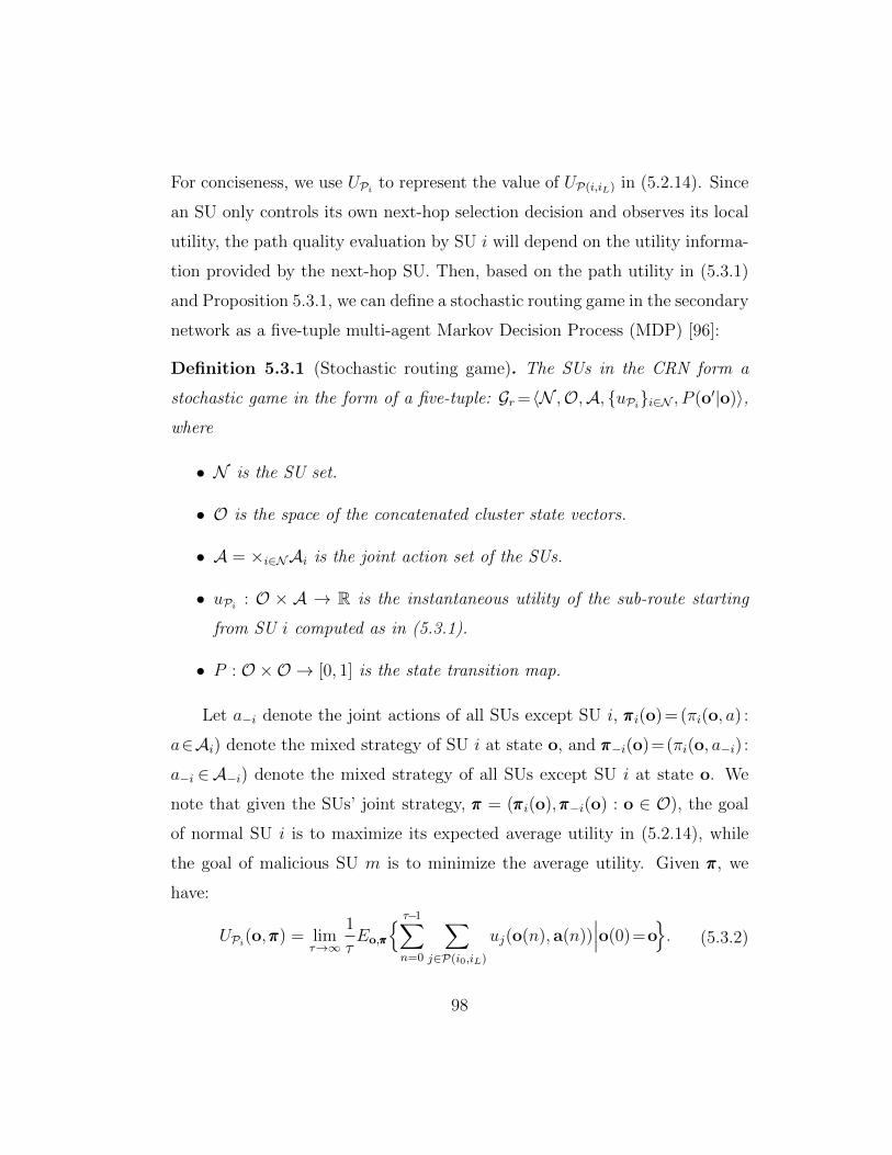
For conciseness, we use UPito represent the value of UP(i,iL) in (5.2.14). Since
an SU only controls its own next-hop selection decision and observes its local
utility, the path quality evaluation by SU i will depend on the utility informa-
tion provided by the next-hop SU. Then, based on the path utility in (5.3.1)
and Proposition 5.3.1, we can define a stochastic routing game in the secondary
network as a five-tuple multi-agent Markov Decision Process (MDP) [96]:
Definition 5.3.1 (Stochastic routing game). The SUs in the CRN form a
stochastic game in the form of a five-tuple: Gr=〈N ,O,A, {uPi}i∈N , P (o′|o)〉,
where
• N is the SU set.
• O is the space of the concatenated cluster state vectors.
• A = ×i∈NAi is the joint action set of the SUs.
• uPi: O × A → R is the instantaneous utility of the sub-route starting
from SU i computed as in (5.3.1).
• P : O ×O → [0, 1] is the state transition map.
Let a−i denote the joint actions of all SUs except SU i, πππi(o) = (πi(o, a) :
a∈Ai) denote the mixed strategy of SU i at state o, and πππ−i(o)=(πi(o, a−i) :
a−i ∈A−i) denote the mixed strategy of all SUs except SU i at state o. We
note that given the SUs’ joint strategy, πππ = (πππi(o),πππ−i(o) : o ∈ O), the goal
of normal SU i is to maximize its expected average utility in (5.2.14), while
the goal of malicious SU m is to minimize the average utility. Given πππ, we
have:
UPi(o,πππ) = lim
τ→∞
1
τEo,πππ
{ τ−1∑n=0
∑j∈P(i0,iL)
uj(o(n), a(n))∣∣∣o(0)=o
}. (5.3.2)
98
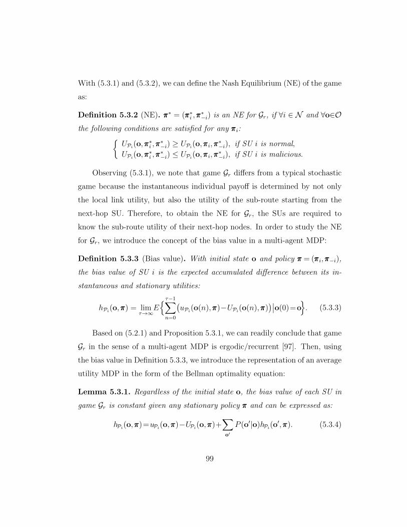
With (5.3.1) and (5.3.2), we can define the Nash Equilibrium (NE) of the game
as:
Definition 5.3.2 (NE). πππ∗ = (πππ∗i ,πππ∗−i) is an NE for Gr, if ∀i ∈ N and ∀o∈O
the following conditions are satisfied for any πππi:{UPi
(o,πππ∗i ,πππ∗−i) ≥ UPi
(o,πππi,πππ∗−i), if SU i is normal,
UPi(o,πππ∗i ,πππ
∗−i) ≤ UPi
(o,πππi,πππ∗−i), if SU i is malicious.
Observing (5.3.1), we note that game Gr differs from a typical stochastic
game because the instantaneous individual payoff is determined by not only
the local link utility, but also the utility of the sub-route starting from the
next-hop SU. Therefore, to obtain the NE for Gr, the SUs are required to
know the sub-route utility of their next-hop nodes. In order to study the NE
for Gr, we introduce the concept of the bias value in a multi-agent MDP:
Definition 5.3.3 (Bias value). With initial state o and policy πππ = (πππi,πππ−i),
the bias value of SU i is the expected accumulated difference between its in-
stantaneous and stationary utilities:
hPi(o,πππ) = lim
τ→∞E{τ−1∑n=0
(uPi
(o(n),πππ)−UPi(o(n),πππ)
)∣∣o(0)=o}. (5.3.3)
Based on (5.2.1) and Proposition 5.3.1, we can readily conclude that game
Gr in the sense of a multi-agent MDP is ergodic/recurrent [97]. Then, using
the bias value in Definition 5.3.3, we introduce the representation of an average
utility MDP in the form of the Bellman optimality equation:
Lemma 5.3.1. Regardless of the initial state o, the bias value of each SU in
game Gr is constant given any stationary policy πππ and can be expressed as:
hPi(o,πππ)=uPi
(o,πππ)−UPi(o,πππ)+
∑o′
P (o′|o)hPi(o′,πππ). (5.3.4)
99
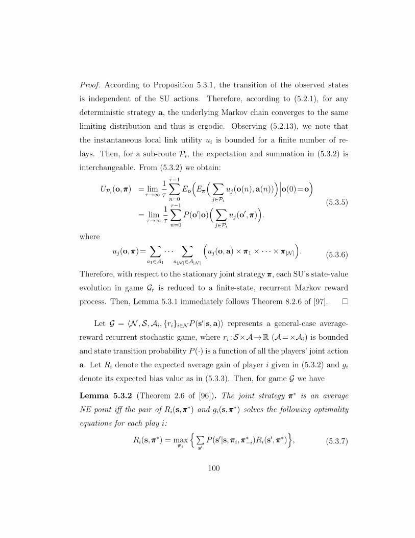
Proof. According to Proposition 5.3.1, the transition of the observed states
is independent of the SU actions. Therefore, according to (5.2.1), for any
deterministic strategy a, the underlying Markov chain converges to the same
limiting distribution and thus is ergodic. Observing (5.2.13), we note that
the instantaneous local link utility ui is bounded for a finite number of re-
lays. Then, for a sub-route Pi, the expectation and summation in (5.3.2) is
interchangeable. From (5.3.2) we obtain:
UPi(o,πππ) = lim
τ→∞
1
τ
τ−1∑n=0
Eo
(Eπππ
(∑j∈Pi
uj(o(n), a(n)))∣∣∣o(0)=o
)= lim
τ→∞
1
τ
τ−1∑n=0
P (o′|o)(∑j∈Pi
uj(o′,πππ)
).
(5.3.5)
where
uj(o,πππ)=∑a1∈A1
· · ·∑
a|N|∈A|N|
(uj(o, a)× πππ1 × · · · × πππ|N |
). (5.3.6)
Therefore, with respect to the stationary joint strategy πππ, each SU’s state-value
evolution in game Gr is reduced to a finite-state, recurrent Markov reward
process. Then, Lemma 5.3.1 immediately follows Theorem 8.2.6 of [97].
Let G = 〈N ,S,Ai, {ri}i∈NP (s′|s, a)〉 represents a general-case average-
reward recurrent stochastic game, where ri :S×A→R (A=×Ai) is bounded
and state transition probability P (·) is a function of all the players’ joint action
a. Let Ri denote the expected average gain of player i given in (5.3.2) and gi
denote its expected bias value as in (5.3.3). Then, for game G we have
Lemma 5.3.2 (Theorem 2.6 of [96]). The joint strategy πππ∗ is an average
NE point iff the pair of Ri(s,πππ∗) and gi(s,πππ
∗) solves the following optimality
equations for each play i:
Ri(s,πππ∗) = max
πππi
{∑s′P (s′|s,πππi,πππ∗−i)Ri(s
′,πππ∗)}, (5.3.7)
100
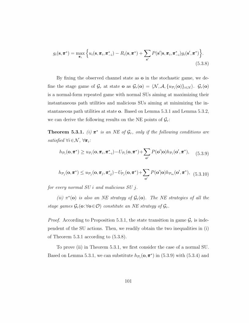
gi(s,πππ∗) = max
πππi
{ui(s,πππi,πππ
∗−i)−Ri(s,πππ
∗) +∑s′
P (s′|s,πππi,πππ∗−i)gi(s′,πππ∗)}.
(5.3.8)
By fixing the observed channel state as o in the stochastic game, we de-
fine the stage game of Gr at state o as Gr(o) = 〈N ,A, {uPi(o)}i∈N 〉. Gr(o)
is a normal-form repeated game with normal SUs aiming at maximizing their
instantaneous path utilities and malicious SUs aiming at minimizing the in-
stantaneous path utilities at state o. Based on Lemma 5.3.1 and Lemma 5.3.2,
we can derive the following results on the NE points of Gr:
Theorem 5.3.1. (i) πππ∗ is an NE of Gr, only if the following conditions are
satisfied ∀i∈N , ∀πππi:
hPi(o,πππ∗) ≥ uPi
(o,πππi,πππ∗−i)−UPi
(o,πππ∗)+∑o′
P (o′|o)hPi(o′,πππ∗), (5.3.9)
hPj(o,πππ∗) ≤ uPj
(o,πππj,πππ∗−j)−UPj
(o,πππ∗)+∑o′
P (o′|o)hPm(o′,πππ∗), (5.3.10)
for every normal SU i and malicious SU j.
(ii) π∗(o) is also an NE strategy of Gr(o). The NE strategies of all the
stage games Gr(o :∀o∈O) constitute an NE strategy of Gr.
Proof. According to Proposition 5.3.1, the state transition in game Gr is inde-
pendent of the SU actions. Then, we readily obtain the two inequalities in (i)
of Theorem 5.3.1 according to (5.3.8).
To prove (ii) in Theorem 5.3.1, we first consider the case of a normal SU.
Based on Lemma 5.3.1, we can substitute hPi(o,πππ∗) in (5.3.9) with (5.3.4) and
101
obtain ∀πππi:
uPi(o,πππ∗)−UPi
(o,πππ∗)+∑o′
P (o′|o)hPi(o′,πππ∗) ≥
uPi(o,πππi,πππ
∗−i)−UPi
(o,πππ∗)+∑o′
P (o′|o)hPi(o′,πππ∗).
(5.3.11)
From (5.3.11) we obtain uPi(o,πππ∗)≥ uPi
(o,πππi,πππ∗−i),∀πππi, which is exactly the
same as the condition equation for an NE in game Gr(o). For a malicious SU
j, we can derive uPj(o,πππ∗) ≤ uPj
(o,πππj,πππ∗−j) similarly with the help of (5.3.10)
in Theorem 5.3.1.
To show that the NE strategies for the stage game group Gr(o : ∀o ∈ O)
constitute an NE strategy for Gr, we rewrite (5.3.5) as follows:
UPi(o,πππ) = lim
τ→∞
1
τ
(τ−1∑n=0
P (o′|o)uPi(o′,πππ)
). (5.3.12)
Consider the case that πππ is comprised of the NE strategies of the stage game
groups, πππ = (πππ∗(o) : ∀o ∈ O). If πππ is not an NE strategy of game Gr, according
to Definition 5.3.2, we can find at least one SU i (assume that SU i is normal),
satisfying the following inequality:
UPi(o,πππ)− UPi
(o, πππi,πππ−i) < 0,∃πππi. (5.3.13)
Then, after substituting UPiin (5.3.13) with (5.3.12), we have:
limτ→∞
1
τ
( τ−1∑n=0
P (o′|o)×(uPi
(o′,πππ∗(o′))− uPi(o′, πππi(o
′),πππ∗−i(o′))))
< 0,
(5.3.14)
which contradicts the fact that πππ∗(o) is the NE strategy of stage game Gr(o).
Therefore, property (ii) of Theorem 5.3.1 holds.
102
Remark 5.3.1. Theorem 5.3.1 establishes the equivalence between the NE
strategies of Gr and the group of NE strategies for its corresponding stage
games. It is worth noting that Theorem 5.3.1 is based on Proposition 5.3.1.
In this case, all the stochastic game NE are the stationary Markov perfect
equilibria. In contrast, for a general case stochastic game where the state
transition is usually a function of the player actions, equality in (5.3.4) may
not hold except for the equilibrium strategies, and the second property in
Theorem 5.3.1 does not exist.
Due to the information flooding overhead, it is unrealistic for the SUs
to frequently exchange the information about their private actions and util-
ities with SUs that are beyond their one-hop neighbors. To determine the
level of information exchange in the routing game, we consider another multi-
agent MDP based on each SU’s local utility ui. We define the MDP as
Gl = 〈N ,O,A, {ui}i∈N , P (o′|o)〉. Let hi(o,πππ) denote the bias value of Gl and
Ui(o,πππ) denote the average gain of Gl. Then, we can show that Lemma 5.3.1
also applies to hi and Ui in Gl. Let πππi,1 denote SU i’s strategy for selecting the
next hop, πππi,2 denote the strategy of SU i for selecting the transmit channel,
and Pai,1 denote the sub-route in Pi starting from the node that is chosen by
SU i with action ai,1. Based on Lemma 5.3.1 and Theorem 5.3.1, we can show
in the following theorem that Gr can be decomposed into a layered multi-agent
MDP:
Theorem 5.3.2. (i) With stationary joint policy πππ, the relay selection process
of SU i can be expressed as (5.3.15).
hPi(o,πππ)+UPi
(o,πππ) = ui(o,πππ)+∑o′P (o′|o)hi(o
′,πππ)
+Eπππi,1
{uPai,1
(o, ai,1,πππi,2,πππ−i)+∑o′P (o′|o)hPai,1
(o, ai,1,πππi,2,πππ−i)}.
(5.3.15)
103
(ii) Strategy πππ is an NE point of Gr when for any normal SU i and mali-
cious SU j, πππi=arg maxπππi
(hPi(o,πππi, πππ−i)+UPi
(o,πππi, πππ−i)),
πππj =arg minπππj
(hPj(o,πππj, πππ−j)+UPj
(o,πππj, πππ−j)).(5.3.16)
Proof. After exchanging the order of expectation and summation, we can ex-
pand (5.3.2) as:
UPi(o,πππ) = lim
τ→∞
1
τ
τ−1∑n=0
Eo
(ui(o(n),πππ)
∣∣∣o(0)=o)
+
Eπππi,1
{limτ→∞
1
τ
τ−1∑n=0
Eo
(uPai,1
(o(n), ai,1,πππi,2,πππ−i)∣∣∣o(0)=o
)}=Ui(o,πππ)+Eπππi,1
{UPai,1
(o, ai,1,πππi,2,πππ−i)},
(5.3.17)
where πππi,1 is SU i’s strategy for choosing the next-hop SU. From (5.3.3) and
(5.3.17), we obtain:
hPi(o,πππ) = lim
τ→∞
τ−1∑n=0
Eo
{ui(o(n),πππ)+Eπππi,1
{uPai,1
(o(n), ai,1,πππi,2,πππ−i)}
−Ui(o,πππ)−Eπππi,1
{UPai,1
(o, ai,1,πππi,2,πππ−i))} ∣∣∣o(0) = o
}= lim
τ→∞
τ−1∑n=0
Eo
{ui(o(n),πππ)− Ui(o,πππ)
∣∣∣o(0) = o
}+ lim
τ→∞
τ−1∑n=0
Eo,πππi,1
{uPai,1
(o(n), ai,1,πππi,2,πππ−i))− UPai,1(o, ai,1,πππi,2,πππ−i))
∣∣∣o(0)=o
}= hi(o,πππ) + Eπππi,1
{hPai,1
(o, ai,1,πππi,2,πππ−i)}.
(5.3.18)
Adding (5.3.17) and (5.3.18), we obtain:
hPi(o,πππ) + UPi
(o,πππ) = hi(o,πππ) + Ui(o,πππ)+
Eπππi,1
{hPai,1
(o, ai,1,πππi,2,πππ−i)+UPai,1(o, ai,1,πππi,2,πππ−i)
}.
(5.3.19)
104
After applying Lemma 5.3.1 to (5.3.19), (5.3.15) is obtained.
Consider a normal SU i ∈ N . From (5.3.4), we can show that the best
response of SU i to the joint strategy πππ−i with respect to the sum of its bias
value and gain value is obtained when
hPi(o, πππ) + UPi
(o, πππ) = maxπππi
(uPi
(o,πππi, πππ−i) +∑o′P (o′|o)hPi
(o, πππ)),
(5.3.20)
where πππ is the solution to the right-hand side of (5.3.20). From (5.3.7) and
(5.3.8) in Lemma 5.3.2, we have
hPi(o,πππ∗) + max
δδδUPi
(o, δδδ,πππ∗−i) = maxπππi
(uPi
(o,πππi,πππ∗−i) +
∑o′P (o′|o)hPi
(o,πππ∗)),
(5.3.21)
and πππ∗ = (δδδ∗,πππ∗−i) is the NE strategy. For the malicious SUs, a similar pair
of equations to (5.3.20) and (5.3.21) can be obtained by substituting operator
max(·) with min(·) in (5.3.20) and (5.3.21). Comparing the right-hand side of
(5.3.20) and (5.3.21), it is straightforward to show that the best response with
respect to hPi(o,πππ) + UPi
(o,πππ) is also the NE strategy of the game.
Remark 5.3.2. Theorem 5.3.2 shows that given a stationary joint policy
πππ, the relay-selecting process of an SU is composed of two value iteration
processes in the form of the Bellman optimality equation. The first process
is determined by the local multi-agent MDP Gl, and the second process is
determined by the sub-path starting from the selected next-hop SU ai,1 in Gr.Furthermore, the second Bellman optimality equation for SU ai,1 can also be
decomposed into the same two-layer form as (5.3.15) with respect to its own
decision on a next-hop selection.
According to Theorem 5.3.2, to derive its local NE strategy πππ∗i , SU i
needs its neighbor nodes j ∈Ni\{i} to truthfully provide the information on
105
the equilibrium value of hPj(o, ai,1 =j,πππi,2,πππ
∗−i)+UPj
(o, ai,1 =j,πππi,2,πππ∗−i). This
requires that the NE for game Gr is solved through backward induction. Ob-
serving (5.3.2) and (5.3.3), it is straightforward to show that when stochastic
game Gr is reduced to a stage game Gr(o) with a single state o, providing the
value hPj(o, ai,1 = j,πππi,2,πππ
∗−i)+UPj
(o, ai,1 = j,πππi,2,πππ∗−i) is equivalent to provid-
ing the value uPj(o, ai,1 = j,πππi,2,πππ
∗−i). Such an observation paves the way for
developing a strategy-learning method based on limited information exchange
between the SUs.
5.3.2 Stochastic strategy learning based on truthfulinformation exchange
According to Theorem 5.3.1, an NE for the stochastic routing game can be
constructed based on the state-dependent NE strategies for each stage routing
game with fixed estimated channel states. Therefore, we consider a stage
routing game at state o: Gr(o) = 〈N ,A, {uPi(o)}i∈N 〉, where uPi
(o, a) =
ui(o, a)+uPai,1(o, a). Based on Theorem 5.3.2, the NE for Gr(o) is achieved
when each normal SU i and malicious SU j play by strategies πππ∗ that satisfy
the following condition:U∗Pi
= maxπππi
(ui(o,πππi,πππ
∗−i) + Eπππi,1
{uPai,1
(o, ai,1,πππi,2,πππ∗−i)})
,
U∗Pj= min
πππj
(uj(o,πππm,πππ
∗−j) + Eπππj,1
{uPaj,1
(o, aj,1,πππj,2,πππ∗−j)})
.(5.3.22)
To avoid information flooding, we assume that the SUs do not share with
their neighbors the local action information. An SU is only able to share its
value of actions by exchanging routing request (RREQ) and routing response
(RREP) packets with its neighbors. In this section, we consider that malicious
SUs do not provide distorted information. Since an SU cannot observe other
106
nodes’ actions, we resort to reinforcement learning to obtain the NE under
the condition of incomplete information. We assume that a stationary joint
strategy πππ is adopted by the SUs in game Gr(o). Then, we consider the
following action-value learning process for SU i:
un+1Pi
(o, ai) = unPi(o, ai) + α(n)I(ai(n), ai)
(uPi
(o, ai(n), a−i(n))−unPi(o, ai)
),
(5.3.23)
where unPi(o, ai) is the expected path utility learned for action ai at slot n, and
0<α(n)<1 is a sequence of learning rates. According to reinforcement learn-
ing theory [48], if uPi(o, ai(n), a−i(n)) is perfectly known by SU i, unPi
(o, ai)
converges almost surely to the real value of uPi(o, ai,πππ−i), given that all the
possible action combinations are visited infinitely often by the SUs and α(n)
satisfies the conditions∑
n α(n) =∞ and∑
n α2(n) <∞.
We first assume that an SU i is able to timely calculate the instantaneous
accumulated utility of path Pi based on its local observation of ui(o(n), a(n))
and the instantaneous sub-path utility uPai,1(o(n), a(n)), which is fed back by
its next-hop SU j = ai,1. In this case, (5.3.23) can be adopted by each SU
to estimate their action value in stage game Gr(o). Then, we can adopt the
Stochastic Fictitious Play (SFP) algorithm [49] for SU i to learn πππi(o, ai,πππ−i):
πππn+1i (o, ai)=πππni (o, ai)+β(n)(BR(unPi
(o), ai)−πππni (o, ai)
), (5.3.24)
where unPi(o) is the vector of utilities unPi
(o, ai) for all action ai at time slot n,
and BR(·) is the perturbed best response strategy of SU i for action ai in the
form of the Logit function:
BR(unPi
(o), ai)
=
exp(λi(unPi
(o, ai)))∑
b∈Aiexp
(λi(unPi
(o,b))) , i is normal,
exp(λi(unPi
(o, ai))−1)
∑b∈Ai
exp(λi(unPi
(o,b))−1) , i is malicious.
(5.3.25)
107
The utility learning process in (5.3.23) and the SPF-based strategy learning
process in (5.3.24) and (5.3.25) form a two timescale learning scheme. From
[48], we introduce Lemma 5.3.3 in regard to the two timescale learning process
given in (5.3.23)-(5.3.25):
Lemma 5.3.3 (Theorem 5 of [48]). Consider that in the following stochastic
approximation processes{θn+11 = θn1 + γn1 (F1(θ
n1 , θ
n2 ) +Mn+1
1 ),
θn+12 = θn2 + γn2 (F2(θ
n1 , θ
n2 ) +Mn+1
2 ),(5.3.26)
for each i, θni are bounded,∑
n→∞ γni = ∞,
∑n→∞(γni )2 < ∞, Fi is globally
Lipschitz continuous, {∑k
n=1 γni M
ni }k converges almost surely, and limn→∞ γ
n1 /γ
n2 =
0. Suppose that for each θ1 the Ordinary Differential Equation (ODE)
dY
dt= F2(θ1, Y ),
has a unique global asymptotically stable equilibrium point ξ(θ1) such that ξ is
Lipschitz continuous. Then almost surely,
limn→∞
‖θn2 − ξ(θn1 )‖ = 0,
and a suitable interpolation of the process {θn1} is an asymptotic pseudo-
trajectory of the flow defined by the ODE
dX
dt= F1(X, ξ(X)).
From [34,49], we introduce Lemma 5.3.4, Lemma 5.3.5 and Lemma 5.3.6,
which further pave the way of studying the convergence property of the pro-
posed learning scheme:
108
Lemma 5.3.4 (Proposition 3.1 of [49]). Consider a general, normal-form
repeated game G = 〈N ,×i∈NAi, {ui}i∈N 〉. Let πni be the fixed point of the
SFP dynamic given by (5.3.29) with respect to a perturbation vector vn =
(vn1 , . . . , vn|N |). If the perturbation sequence {vn} converges weakly, and the
sequence {πni } converges to π∗i , then π∗i is the NE for G.
Lemma 5.3.5 (Supermodular game [34]). A continuous normal-form game
G = 〈N , {ΠΠΠi}i∈N , {ui(πππi)}i∈N 〉 is a supermodular game if for any player i ∈ N ,
i) the strategy space ΠΠΠi is a compact subset of RK.
ii) the payoff function ui is upper semi-continuous in πππi = (πππi,πππ−i).
iii) ∂2ui(πππ)∂πππi,k∂πππj,l
≥ 0 ∀j 6= i, k, l, where πππi,k is the k-th element of vector πππi.
Lemma 5.3.6 (Corollary 5.5 of [49]). If a generic repeated game G is a super-
modular game, then the solutions to the smooth best response dynamic in the
form of (5.3.29) for G converges almost surely to its rest point set from any ini-
tial condition. The remaining nonconvergent initial conditions are contained
in a finite or countable union ∪iMi, of invariant manifolds of codimension 1,
and hence have measure zero.
With the help of Lemmas 5.3.3-5.3.6, we can prove that the two timescale
learning scheme has the following convergence property:
Theorem 5.3.3. If uPi(o, a(n)) is known to each SU at every time slot, and
the following conditions are satisfied: limn→∞
∑n α(n) = ∞, lim
n→∞
∑n α
2(n) <
∞, limn→∞
∑n β(n) =∞, lim
n→∞
∑n β
2(n) <∞ and limn→∞
(β(n)/α(n)) = 0, then,
{πππni (o, ai)} as given by the learning process (5.3.23)-(5.3.25) converges almost
surely to an NE for stage game Gr(o).
109
Proof. Let {unPi(o, ai)} in (5.3.23) be {θn2} in (5.3.26) and {πππni (o)} in (5.3.24)
be {θn1} in (5.3.26), then we define the following two ODEs:
duPi(o, ai)
dt=F2(uPi
, πππi)=uPi(o, ai)−uPi
(o, aPi), (5.3.27)
dπππi(o, ai)
dt=F1(uPi
, πππi)=BR(uPi(o))−πππi(o, ai). (5.3.28)
According to our discussion on (5.3.23), uPi(o, ai) almost surely converges to
uPi(o, ai,πππ−i). Then, by Lemma 5.3.3, a suitable interpolation of {πππni (o)} is
an asymptotic pseudo-trajectory of the flow defined by the ODE in (5.3.28).
It is known (see [48,49]) that (5.3.28) is equivalent to (5.3.29):
dπππi(o)
dt= BR(πππ−i(o))− πππi(o), (5.3.29)
where for a normal SU i (we omit the state indicator o for simplicity)
BR(πππ−i)=arg maxπππi
(uPi
(πππi,πππ−i)−λi∑ai
πππi(ai) logπππi(ai)), (5.3.30)
and for a malicious SU j
BR(πππ−j)=argmaxπππj
(u−1Pj
(πππj,πππ−j)−λj∑aj
πππj(aj)logπππj(aj)), (5.3.31)
because (5.3.25) provides the solutions to (5.3.30) and (5.3.31) [49]. In (5.3.30)
and (5.3.31), the entropy function vi(πππi) = −∑
aiπππi(ai) logπππi(ai) is called the
perturbation in SFP.
By Lemma 5.3.4, when the solution to the ODE in (5.3.29) converges to
a fixed point, which in this case is by definition the NE of game Gr(o). Then,
based on the discussion following Lemma 5.3.3, proving the convergence of the
learning process given by (5.3.23)-(5.3.25) to the NE is equivalent to proving
that the solution trajectories to the SFP dynamic in (5.3.28) converges to a
110
set of fixed points from any initial condition. Observing the structure of Gr(o),
the proof can be developed using the following properties of a repeated game:
With Lemma 5.3.5, we can check the supermodularity of game Gr(o) with
respect to strategy πππi. According to (5.2.13) we have ui ≥ 0 ∀o, a. Then,
according to (5.3.6), ∀i 6= j
∂2(uPi=∑
i∈Piui(πππ))
∂πππi(ai)∂πππj(aj)≥ 0,∀ai, aj. (5.3.32)
Therefore, game Gr(o) in the form of continuous game7 with strategy πππ is
a supermodular game. By Lemma 5.3.6, the smooth best response dynamic
converges almost surely. By Lemma 5.3.4, Theorem 5.3.3 is proved.
Although the learning scheme given by (5.3.24) and (5.3.25) possesses
good convergence property, the assumption of perfectly knowing the instanta-
neous path utility is fairly strict. It requires a large amount of signaling to be
completed within a single time slot. To address such a problem, we relax the
requirement on information exchange by assuming that SU i only shares its
locally estimated value of uPi(o,πππ) with its neighbors. Based on the discussion
for (5.3.23), it is obvious that an SU can learn its expected local link utility
ui(o, ai,πππ−i) through an iteration which is similar to (5.3.23), as long as all
possible joint actions are visited infinitely often:
un+1i (o, ai) = uni (o, ai)+α(n)I(ai(n), ai) (ui(o, a(n))−uni (o, ai)) . (5.3.33)
Using the value of uni (o, ai) and the value of unPai,1(o) provided by the next-hop
7It is easy to check that the property also holds for malicious SUs as long as their strategylearning scheme complies with SFP given by (5.3.25).
111
SU j = ai,1, we introduce the learning scheme for uPi(o,πππ):
un+1Pi
(o) = unPi(o) + γi(n)
(∑ai
πππni (o, ai)(uni (o, ai) + unPai,1
(o))−unPi
(o)).
(5.3.34)
We also modify the learning scheme of (5.3.24) and obtain:
πππn+1i (o, ai)=πππni (o, ai) + β(n)
(BR(uni (o, ai) + unPai,1
(o), ai)− πππni (o, ai)
),
(5.3.35)
where BR(·) is the modified perturbed best response strategy:
BR(uni (o) + unPai,1
(o), ai
)=
exp(λi(ui(o, ai) + unPai,1
(o)))
∑b∈Ai
exp(λi(ui(o,b) + unPai,1
(o))) , i is normal,
exp(λi(ui(o, ai) + unPai,1
(o))−1)
∑b∈Ai
exp(λi(ui(o,b) + unPai,1
(o))−1) , i is malicious.
(5.3.36)
The learning scheme defined by (5.3.33)-(5.3.36) does not require SU i
to immediately report an instantaneous path utility to its previous-hop SU.
However, comparing (5.3.34) with (5.3.22), we note that (5.3.34) provides a
biased estimation of uPi(o,πππ), given that πππni converges. Since the learned path
utility in (5.3.34) is a biased estimation, the new learning scheme can only
obtain an approximation of the NE point of the stage game. The convergence
condition for the learning scheme given by (5.3.33)-(5.3.36) is provided in
Theorem 5.3.4.
Theorem 5.3.4. Assume that the following are satisfied:
limn→∞
∑n
α(n) =∞, limn→∞
∑n
α2(n) <∞, limn→∞
∑n
γi(n) =∞, limn→∞
∑n
γ2i (n) <∞,
limn→∞
∑n
β(n)=∞, limn→∞
∑n
β2(n)<∞, limn→∞
(γi(n)/α(n))=0, limn→∞
(β(n)/γi(n))=
112
0, and limn→∞
(γi(n)/γj(n)) = 0, if SU i is closer to the sink SU than SU j in
terms of distance. Then, {πππni (o, ai)} obtained through the learning process
(5.3.33)-(5.3.36) converges almost surely.
Proof. The proof of Theorem 5.3.4 can be achieved by repeatedly applying
Lemma 5.3.3 to the learning scheme given by (5.3.33) and (5.3.34), then to the
learning scheme given by (5.3.34) and (5.3.35). According to our discussion
on (5.3.33), uni (o, ai) has a unique global asymptotically stable equilibrium
ui(o, ai,πππ−i) if πππ is fixed. Then, it is sufficient to prove that the following
ODE:
duPi(o)
dt=(∑
ai
πππi(o, ai)(ui(o, ai)+uPai,1(o))−uPi
(o)), (5.3.37)
is globally asymptotically stable to show that the learning process given by
(5.3.33)-(5.3.35) produces an asymptotic pseudo-trajectory of the SFP flow.
Omitting state indicator o for convenience, we denote uPi(ai)= ui(ai)+uPai,1
,
ξi=duPidt
and ε(ai)=duPi (ai)
dt, and define a Lyapunov function:
Vi(t) =(∑
ai
πππi(ai)(ui(ai)+uPai,1
)−uPi
)2. (5.3.38)
We sort the SUs in path Pi according to their distance in hop count to sink L in
an ascending order as {L−1, L−2, . . . , i}. Then, the two-timescale stochastic
approximation process in Lemma 5.3.3 can be extended to multiple-timescale
with the same form of function Fi as in (5.3.26):
F1(uj(aj), πππ) = uj(aj(n))− unj (aj),
and
F j2 (uj(aj), uPj
, uPj+1)=∑ai
πππi(ai)(ui(ai)+uPaj)−uPi .
113
Since the learning process in (5.3.33) is globally asymptotically convergent,
then at the stable point of ui,duidt
=0 and εi(ai)=duPi+1
dt, where ai,1 = i+1. We
now examine Vi and obtain
1
2
dVidt
=(∑
ai
πππi(ai)uPi(ai)−uPi
)×
(d
dt
∑ai
eλiuPi (ai)∑b e
λiuPi (b)uPi
(ai)−duPi
dt
),
=ξi
(∑ai
(∑b
λieλiuPi (ai)uPi (b)(∑b e
λiuPi (b))2 (εi(ai)−εi(b))uPi
(ai) +eλiuPi (ai)∑b e
λiuPi (b)εi(ai)
)−ξi),
=λi∑ai
∑b
eλiuPi (ai)∑b e
λiuPi (b)(εi(ai)−εi(b))uPi
(ai)ξi +∑ai
eλiuPi (ai)∑b e
λiuPi (b)εi(ai)ξi−ξ2i .
We start by examining the property of dVidt
as a backward propagation
from SU L− 1. Since uPL=0, we have εL−1(aL−1)=0, hence 1
2
dVL−1dt
=−ξ2L−1≤0
at the stable point of the approximation process represented by FL−12 (uL−1, πππ).
Therefore, the ODE for SU L − 1 in the form of (5.3.37) is globally asymp-
totically convergent. Then, we can apply Lemma 5.3.3 to the two-timescale
learning process formed by FL−12 and FL−2
2 , and show that a suitable interpo-
lation of the process {unPL−2} is an asymptotic pseudo-trajectory of the flow
defined by the ODEduPL−2
dtgiven in (5.3.37). At the stable point of uPL−1
, we
haveduPL−1
dt=0, so εL−2(aL−2)=0. Following a similar way to analyze dVL−1
dt, we
have 12
dVL−2
dt=−ξ2L−2≤0. By repeatedly applying the same analysis to the se-
quence of the learning processes {(FL−12 , FL−2
2 ), (FL−22 , FL−3
2 ), . . . , (F i+12 , F i
2)},
we obtain Proposition 5.3.2:
Proposition 5.3.2. The learning process given in (5.3.33) and (5.3.34) is
globally asymptotically convergent, provided that the following are satisfied:
limn→∞
∑n
α(n) =∞, limn→∞
∑n
α2(n) <∞, limn→∞
∑n
γi(n) =∞, limn→∞
∑n
γ2i (n) <∞,
limn→∞
(γi(n)/α(n)) = 0 and limn→∞
(γi(n)/γj(n)) = 0, if SU i is closer in terms of
hop count to the sink SU than SU j.
114
If limn→∞
(β(n)/γi(n))=0, we can further conclude that the learning process
given by (5.3.35) and (5.3.36) generates an asymptotic pseudo-trajectory of
the flow defined by the SPF-based ODE. We note that Lemma 5.3.6 and
Lemma 5.3.5 still hold for a new game with the utility of each player being
the convergent biased value estimation. Then, Theorem 5.3.4 is proved.
5.3.3 Truth-telling enforcement through multi-armbandit
Now, we consider the situation when the malicious SUs also perform the SH
attacks. In this case, the malicious SUs may distort the value of uPi(o) and
report an estimated utility which is much larger than the real value to their
neighbor SUs. As a result, a normal neighbor with strategy learning scheme
in (5.3.35) will choose a malicious SU as its relay with a higher probability.
Then, the malicious SU will induce the neighbor SUs to forward more packets
to itself. To address this situation, we introduce a feedback mechanism for a
relay SU to measure the real delay associated with the path that it chooses
toward a sink SU. We consider that a normal relay SU i is able to insert a
Request-ACK packet into the flows that it serves in random time intervals.
SU i records the time stamp for sending the Request-ACK packet. When
receiving the Request-ACK packet, the corresponding sink SU L replies with
a Response packet to SU i by including the time stamp for reception in the
packet. We assume that the data in the Response packet is protected by a
pair of keys and is always reliable. With the two time stamps, SU i is able to
calculate the total delay time of the Request-ACK packet over the sub-path
through the next-hop SU j = ai,1 that it chooses with action ai. Let ci(ai)
denote such a delay measured by SU i. Then, SU i needs to evaluate the
115
trustworthiness of its next-hop SU j based on sequence {cni (ai(n))}, where n
is a time slot for SU i to send a Request-ACK packet.
We consider that with a certain termination condition, the learning scheme
given in (5.3.33)-(5.3.36) can always reach a stationary policy πππ. Meanwhile,
a malicious SU m shares a fixed distorted value of uPm(o) with the neighbors.
From the perspective of a normal SU i, when sending a Request-ACK packet,
its relay selection can be considered as a Multi-Arm Bandit (MAB) [98] pro-
cess, since at slot n SU i can choose only one neighbor as its relay according
to ai,1(n), and only the real path delay through relay node ai,1(n) can be
confirmed. We note that the real path delay (i.e., the cost of each arm) is a
stochastic function determined by stationary distribution πππ, while the arm se-
lection sequence is generated by the local strategy πππi. Formally, we can define
the MAB for trustworthiness evaluation as follows:
Definition 5.3.4. For each normal SU i, the MAB for trustworthiness evalua-
tion in state o can be defined by a 4-tuple: Bi = 〈Ai, {cni (o, ai(n))}n, {x(n)}n, {n}〉,
where
• Ai is the set of the single-bandit processes and corresponds to the set of
actions of SU i.
• {cni (o, ai(n))}n is the sequence of costs.
• {x(n)=ai(n)}n is the sequence of relay (i.e., arm) selection decisions.
It is worth noting that the MAB given in Definition 5.3.4 differs from
a typical MAB in that the sequence of arm selection {x(n)}n is generated
following a given policy πππi. Therefore, we can consider the MAB process up
to time slot n as a utility exploration phase with a given sampling distribution
116
πππi. With the MAB given in Definition 5.3.4, SU i is able to calculate the
accumulated delay for the Request-ACK packets that it sends with action
ai(n) = a:
Cni (o, a) =
{cni (o, ai(n)) + Cn−1
i (o, a) if n ∈ {n}, ai(n) = a
Cn−1i (o, a), otherwise,
(5.3.39)
and the empirical (sampled) frequency of each action is:
Zn(o, a) =1
n(I(ai(n), a) + (n− 1)Zn−1(o, a)). (5.3.40)
With (5.3.39) and (5.3.40), we can obtain the sampled average path delay
of SU i at action a(n) = a as Rni (o, a) = Cn
i (o, a)/Zni (o, a). Then according
to [98], a greedy, sub-optimal mixed strategy for arm allocation to minimize
the average path delay can be obtained using the Logit function:
σni (o, a) =exp
(λi(R
ni (o, a))−1
)∑b∈Ai
exp(λi (Rn
i (o,b))−1) , (5.3.41)
which is in a similar form to (5.3.25). σni (a) does not have to be consistent
with the learned equilibrium policy when every SU is honest. However, it can
represent the trustworthiness ranking value of the relay associated with action
a. During the estimation of the perturbed best response, a normal SU will
consider the contribution of the reported sub-path utilities by its neighbors in
proportion to the trustworthiness credit that it assigns to each neighbor. Ac-
cording to (5.3.30), a normal SU i modifies its smooth best response objective
as follows:
BR(πππ−i)= arg maxπππi
(∑ai
πππi(ai)(ui(o,πππ(ai),πππ−i)+σni (o, ai)uPai,1
(o,πππ))
−λi∑ai
πππi(ai) logπππi(ai)).
(5.3.42)
117
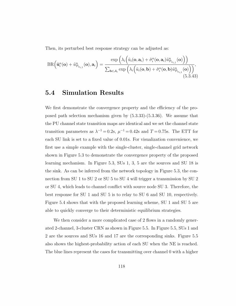
Then, its perturbed best response strategy can be adjusted as:
BR(uni (o) + unPai,1
(o), ai
)=
exp(λi
(ui(o, ai) + σni (o, ai)u
nPai,1
(o)))
∑b∈Ai
exp(λi
(ui(o,b) + σni (o,b)unPai,1
(o))) ,
(5.3.43)
5.4 Simulation Results
We first demonstrate the convergence property and the efficiency of the pro-
posed path selection mechanism given by (5.3.33)-(5.3.36). We assume that
the PU channel state transition maps are identical and we set the channel state
transition parameters as λ−1 = 0.2s, µ−1 = 0.42s and T = 0.75s. The ETT for
each SU link is set to a fixed value of 0.01s. For visualization convenience, we
first use a simple example with the single-cluster, single-channel grid network
shown in Figure 5.3 to demonstrate the convergence property of the proposed
learning mechanism. In Figure 5.3, SUs 1, 3, 5 are the sources and SU 18 is
the sink. As can be inferred from the network topology in Figure 5.3, the con-
nection from SU 1 to SU 2 or SU 5 to SU 4 will trigger a transmission by SU 2
or SU 4, which leads to channel conflict with source node SU 3. Therefore, the
best response for SU 1 and SU 5 is to relay to SU 6 and SU 10, respectively.
Figure 5.4 shows that with the proposed learning scheme, SU 1 and SU 5 are
able to quickly converge to their deterministic equilibrium strategies.
We then consider a more complicated case of 2 flows in a randomly gener-
ated 2-channel, 3-cluster CRN as shown in Figure 5.5. In Figure 5.5, SUs 1 and
2 are the sources and SUs 16 and 17 are the corresponding sinks. Figure 5.5
also shows the highest-probability action of each SU when the NE is reached.
The blue lines represent the cases for transmitting over channel 0 with a higher
118
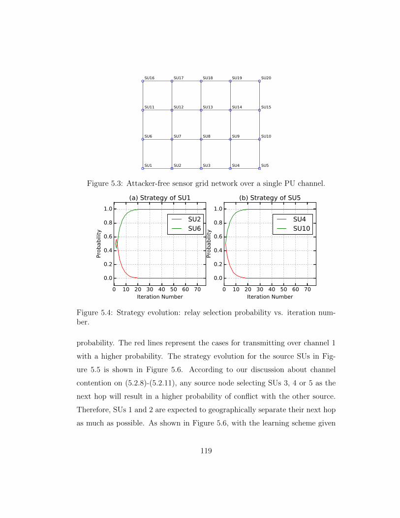
SU1 SU2 SU3 SU4 SU5
SU6 SU7 SU8 SU9 SU10
SU11 SU12 SU13 SU14 SU15
SU16 SU17 SU18 SU19 SU20
Figure 5.3: Attacker-free sensor grid network over a single PU channel.
0 10 20 30 40 50 60 70Iteration Number
0.0
0.2
0.4
0.6
0.8
1.0
Probability
(a) Strategy of SU1
SU2SU6
0 10 20 30 40 50 60 70Iteration Number
0.0
0.2
0.4
0.6
0.8
1.0Probability
(b) Strategy of SU5
SU4SU10
Figure 5.4: Strategy evolution: relay selection probability vs. iteration num-ber.
probability. The red lines represent the cases for transmitting over channel 1
with a higher probability. The strategy evolution for the source SUs in Fig-
ure 5.5 is shown in Figure 5.6. According to our discussion about channel
contention on (5.2.8)-(5.2.11), any source node selecting SUs 3, 4 or 5 as the
next hop will result in a higher probability of conflict with the other source.
Therefore, SUs 1 and 2 are expected to geographically separate their next hop
as much as possible. As shown in Figure 5.6, with the learning scheme given
119
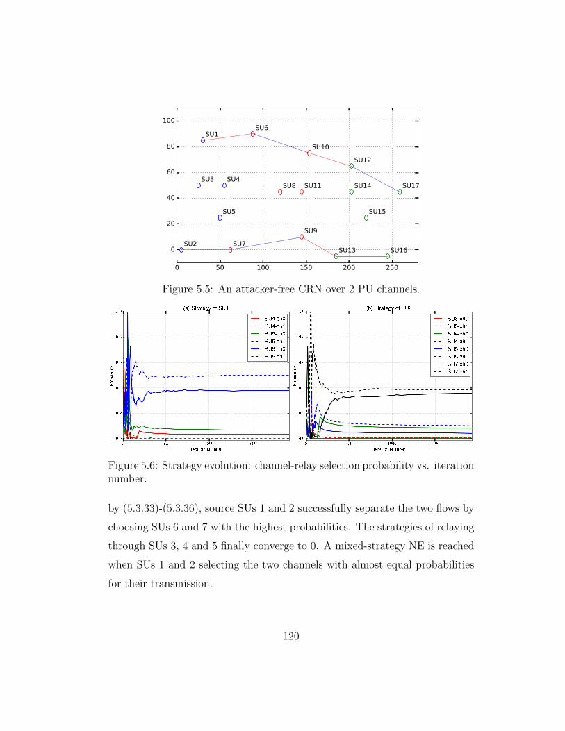
0 50 100 150 200 250
0
20
40
60
80
100
SU1
SU2
SU3 SU4
SU5
SU6
SU7
SU8
SU9
SU10
SU11
SU12
SU13
SU14
SU15
SU16
SU17
Figure 5.5: An attacker-free CRN over 2 PU channels.
Figure 5.6: Strategy evolution: channel-relay selection probability vs. iterationnumber.
by (5.3.33)-(5.3.36), source SUs 1 and 2 successfully separate the two flows by
choosing SUs 6 and 7 with the highest probabilities. The strategies of relaying
through SUs 3, 4 and 5 finally converge to 0. A mixed-strategy NE is reached
when SUs 1 and 2 selecting the two channels with almost equal probabilities
for their transmission.
120
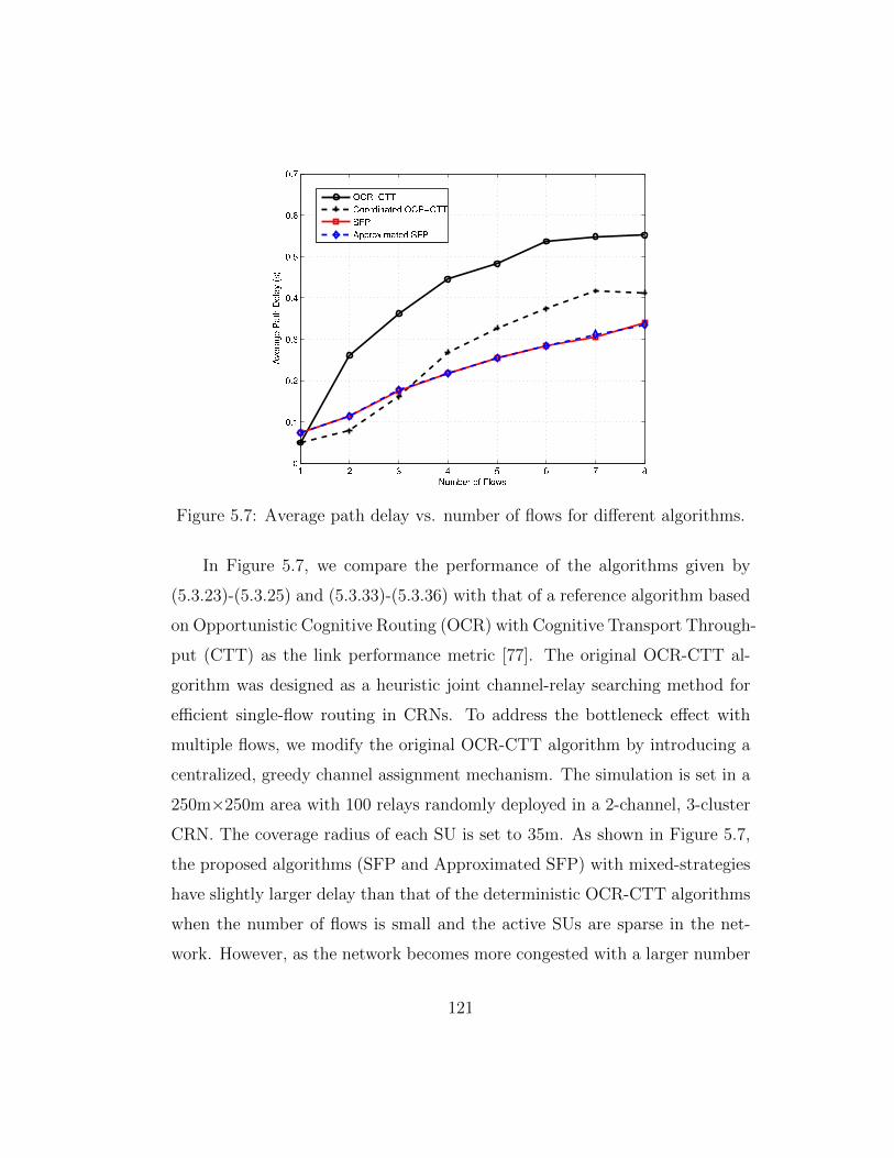
Figure 5.7: Average path delay vs. number of flows for different algorithms.
In Figure 5.7, we compare the performance of the algorithms given by
(5.3.23)-(5.3.25) and (5.3.33)-(5.3.36) with that of a reference algorithm based
on Opportunistic Cognitive Routing (OCR) with Cognitive Transport Through-
put (CTT) as the link performance metric [77]. The original OCR-CTT al-
gorithm was designed as a heuristic joint channel-relay searching method for
efficient single-flow routing in CRNs. To address the bottleneck effect with
multiple flows, we modify the original OCR-CTT algorithm by introducing a
centralized, greedy channel assignment mechanism. The simulation is set in a
250m×250m area with 100 relays randomly deployed in a 2-channel, 3-cluster
CRN. The coverage radius of each SU is set to 35m. As shown in Figure 5.7,
the proposed algorithms (SFP and Approximated SFP) with mixed-strategies
have slightly larger delay than that of the deterministic OCR-CTT algorithms
when the number of flows is small and the active SUs are sparse in the net-
work. However, as the network becomes more congested with a larger number
121
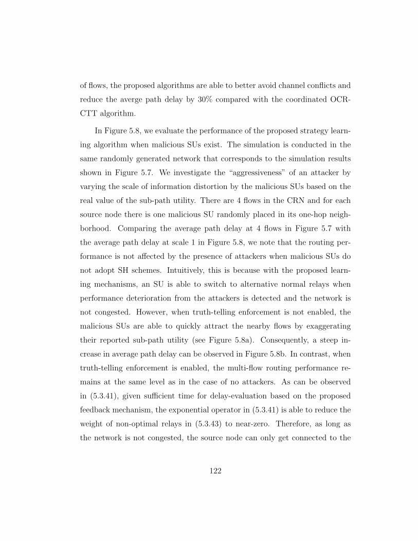
of flows, the proposed algorithms are able to better avoid channel conflicts and
reduce the averge path delay by 30% compared with the coordinated OCR-
CTT algorithm.
In Figure 5.8, we evaluate the performance of the proposed strategy learn-
ing algorithm when malicious SUs exist. The simulation is conducted in the
same randomly generated network that corresponds to the simulation results
shown in Figure 5.7. We investigate the “aggressiveness” of an attacker by
varying the scale of information distortion by the malicious SUs based on the
real value of the sub-path utility. There are 4 flows in the CRN and for each
source node there is one malicious SU randomly placed in its one-hop neigh-
borhood. Comparing the average path delay at 4 flows in Figure 5.7 with
the average path delay at scale 1 in Figure 5.8, we note that the routing per-
formance is not affected by the presence of attackers when malicious SUs do
not adopt SH schemes. Intuitively, this is because with the proposed learn-
ing mechanisms, an SU is able to switch to alternative normal relays when
performance deterioration from the attackers is detected and the network is
not congested. However, when truth-telling enforcement is not enabled, the
malicious SUs are able to quickly attract the nearby flows by exaggerating
their reported sub-path utility (see Figure 5.8a). Consequently, a steep in-
crease in average path delay can be observed in Figure 5.8b. In contrast, when
truth-telling enforcement is enabled, the multi-flow routing performance re-
mains at the same level as in the case of no attackers. As can be observed
in (5.3.41), given sufficient time for delay-evaluation based on the proposed
feedback mechanism, the exponential operator in (5.3.41) is able to reduce the
weight of non-optimal relays in (5.3.43) to near-zero. Therefore, as long as
the network is not congested, the source node can only get connected to the
122
✶ ✶�✶ ✶�✁ ✶�✂ ✶�✄ ✶�☎ ✶�✆ ✶�✝ ✶�✞✵�✁
✵�✁☎
✵�✂
✵�✂☎
✵�✄
✵�✄☎
✵�☎
✵�☎☎
✵�✆
✵�✆☎
❙✟✠✡☛ ☞✌ ✍✎✏✡✏✎✑ ✒✓✠✔✔☛✕✠✎✏☞✖ ✗✑ ✘✠✡✏✟✏☞✙✚ ✛☞✜☛✚
❆✢✣✤✥✣✦✧★✩✪✣✫✧✬✭✮✯
✰✗✱
❙✲✳
✴✷✷✕☞✓✏✸✠✎☛✜ ❙✲✳
✴✷✷✕☞✓✏✸✠✎☛✜ ❙✲✳ ✹ ✒✖✌☞✕✟☛✜ ✺✕✙✎✻ ✺☛✡✡✏✖✔
Figure 5.8: (a) Frequency of connections to malicious nodes vs. scale forutility. (b) Average path delay vs. scale of exaggerated utility by maliciousnodes.
malicious nodes if the routing performance through the malicious nodes is no
worse than the performance through any other neighbor nodes.
123
5.5 Chapter Summary
In this chapter, we have presented a stochastic-learning-based spectrum-aware
relay-selection scheme for the multi-channel, multi-hop cognitive radio network
(CRN), which is robust against the combined Routing-toward-Primary-User
(RPU) and Sink-Hole (SH) attack. By formulating the distributed routing
process as a stochastic game and showing that it can be decomposed into a
group of single-state repeated games, we have introduced the SFP-based relay
selection algorithms with limited information back propagation. To defend the
SH attack, we have also introduced a Multi-Arm Bandit (MAB) based truth-
telling enforcement procedure for normal SUs to evaluate the trustworthiness
of their candidate relays. We have demonstrated in our simulation that the
proposed routing algorithm is able to reduce the average network delay by at
most 50% compared to conventional single-flow routing. The proposed truth-
telling evaluation mechanism guarantees that the proposed routing algorithm
is not affected by the combined attacks.
124
Chapter 6
Summary and Future Work
6.1 Summary
This dissertation studies self-organized learning mechanisms for cross-layer
resource allocation in cognitive wireless networks. Based on the analysis of
dynamic-system optimization and multi-player non-cooperative games, we pro-
pose a series of novel strategy-learning solutions for resource allocation prob-
lems in wireless video streaming, energy-efficient power allocation and robust
spectrum-aware routing. In our study, we emphasize the functionality of au-
tonomous learning and self-organization in cognitive wireless networks. In
contrast to other conventional wireless networks, a cognitive wireless network
is expected to be able to make decisions even in the presence of a lack of knowl-
edge about the network model or a lack of information about other devices’
strategies. Consequently, we propose a model-free strategy learning framework
for the wireless devices to derive their optimal/best-response strategies in the
scenarios of black-box network control.
For the problem of real-time video streaming between a single pair of
125
transmitter and receiver, we propose a two-objective dynamic control model
that consider both the end-to-end distortion and the constraint on allowable
transmission time. By considering the stochastic error propagation, which is
jointly determined by the codec-related data-dependent structure and by the
channel dynamics, we introduce the IR-HARQ scheme for unequal error pro-
tection during video streaming. By jointly modeling the video coding control
and the channel coding control processes with unknown channel dynamics as a
constrained Markov decision problem, we are able to employ R-learning based
strategy learning to derive an optimal transmission control strategy for the
transmitter-receiver pair.
For the problem of energy-efficient power allocation in a two-tier heteroge-
neous network, we model the interactions between the macrocell users and the
femtocell users as a hierarchical game by introducing an interference-pricing
mechanism for the macrocell user. We provide theoretic analysis for both the
case of continuous power space and the case of discrete power space for the
femtocell users and propose two strategy-learning algorithms for the contin-
uous game and the discrete game, respectively. Especially for the discrete
power allocation game, we propose a stochastic learning-based algorithm that
enables the femtocell users to distributively learn their sub-game Nash equi-
librium strategies without the need to know the strategies or payoffs of other
femtocell users. Such a learning scheme is proved to be able to almost surely
converge to the Nash equilibrium with any arbitrary initial transmit power for
the femtocell users.
Next, we study a joint power, channel and base station selection problem
in a self-sustainable network powered by a microgrid with renewable energy
generators. With the electric power supply subsystem imposing a constraint
126
on energy consumption according to the current energy state and estimated
future power demand, we also model the joint resource allocation problem as
a hierarchical game. Instead of modeling the follower subgame as an N -player
noncooperative game, we propose a combinatorial auction mechanism for the
mobile stations in the network to autonomously compete for the subcarrier
sets offered by the base stations through iterative strategy learning. Our sim-
ulations results show that with the mechanism of power pricing, the proposed
learning algorithm is able to improve the operation time of the network based
only on renewable energy by more than 30%.
For the multi-hop multi-channel cognitive radio network, we investigate
the problem of multi-flow spectrum-aware routing under unknown primary-
user channel dynamics. Due to the distributive nature of the multi-hop cog-
nitive radio network, routing protocols are especially vulnerable to insider
attackers that distort information that they report to other nodes to establish
paths. In our study, we model the interactions among SUs as a stochas-
tic game, whose dynamics is also determined by the underlying stochastic
primary-user channel evolution. Based on the Nash equilibrium analysis for
the stochastic game and the corresponding stage repeated games, we propose
a decomposition-based, stochastic learning mechanism for each node in the
network to learn their best-response strategies with limited requirement of
information sharing. To further improve the robustness of the routing mech-
anism against information distortion due to sink-hole attacks, we propose a
feedback-based truth-telling enforcing scheme based on multi-arm bandits. In
comparison with the existing spectrum-aware routing mechanisms for cogni-
tive radio networks, our simulation results show that the proposed algorithm is
able to reduce the network delay by 30% and is able to avoid the performance
127
deterioration due to insider attacks.
6.2 Future Work
Our current research has covered resource allocation problems in small-cell net-
works, OFDMA networks and multi-hop cognitive radio networks. It is worth
noting that the formulation of cross-layer resource allocation problems may
vary with a great degree, depending on the scenarios and the protocol layers
that are considered. As a result, under the framework of model-free strategy-
learning, it is still necessary to carefully design the learning algorithm for each
specific problem and investigate their convergence property and efficiency in
terms of overhead, performance, etc.
Generally, the goal of a perfect self-organized learning mechanism for
multi-agent decision making processes is to achieve self-play (autonomy), sta-
bility and optimality at the same time. However, it has been well-recognized
that for multi-agent learning (more frequently in a stochastic scenario), im-
proving system performance typically incurs more signaling and coordination,
thus undermining the self-play structure. Especially, when learning is imple-
mented under the framework of games, achieving any two goals of self-play,
stability and network optimality is usually at the cost of undermining the
third goal. In recent years, the relation between these three goals in multi-
agent learning has been discussed in many works. However, to our best knowl-
edge most of the discussion only remain at a high-level theoretical perspec-
tive [99–101].
One important issue to be addressed in our current work is the convergence
rate of learning algorithms. Although analytical results for the convergence
128
rate of learning algorithms are highly desired, most of the existing studies are
only able to show empirical results for the learning convergence rate through
numerical simulations. The reason for this is partly due to the asymptotic
convergence condition (such as shown by our studies in Chapters 3 and 5),
which requires for most of the existing learning algorithms that the states and
actions are visited infinitely to ensure the convergence. With such limitation,
one known approach to analyze the convergence speed of a learning scheme
is to view the learning process itself as a discrete time Markov chain. In this
approach, it is possible to apply the standard Markov chain analysis and obtain
the expected time (number of iterations) to learn before reaching the chain’s
absorbing state (e.g., the equilibrium point of a repeated game). However, such
an approach could be computationally intractable when the system/learning
scheme is too complicated, and it is yet to be found applicable to more complex
learning schemes such as those in general-case stochastic games.
Another possible future work is to investigate the possibility of utilizing
the experience acquired through strategy learning in history to new scenarios
or new devices to accelerate the speed of convergence reaching. Although
the experience-sharing framework has been discussed by recent work such as
docitive networks [41, 102] based on the parallel and homogeneous learning
processes, sharing the strategy experiences between heterogeneous learning
processes generally remains an open issue. A natural consideration is to adopt
the Transfer-Learning (TL) paradigm [103], which is design for transferring
knowledge (i.e., experience) from a well-established learning processes (known
as the source task) to a newly established learning process (known as the target
task) working under a different situation. To our best knowledge, few studies
in wireless networks are found discussing such topics. However, discussions
129

on cross-game learning or cross-mechanism learning have already begun in
the area of economic games [104] and automatic control [105]. Although a
detailed discussion on these topics is beyond the scope of this dissertation,
we believe that addressing these issues will bring great improvement to the
existing learning mechanisms for cognitive wireless networks.
130
Bibliography
[1] J. Mitola, Cognitive Radio – An Integrated Agent Architecture for Soft-
ware Defined Radio. PhD thesis, Royal Institute of Technology (KTH),
Kista, Sweden, May 2000.
[2] S. Haykin, “Cognitive radio: brain-empowered wireless communications,”
IEEE Journal on Selected Areas in Communications, vol. 23, pp. 201–
220, Feb 2005.
[3] B. Wang and K. Liu, “Advances in cognitive radio networks: A survey,”
IEEE Journal of Selected Topics in Signal Processing, vol. 5, pp. 5–23,
Feb 2011.
[4] S. Haykin, Cognitive Dynamic Systems: Perception-Action Cycle, Radar
and Radio. Cambridge University Press, 2012.
[5] I. Akyildiz, W.-Y. Lee, M. C. Vuran, and S. Mohanty, “A survey on spec-
trum management in cognitive radio networks,” IEEE Communications
Magazine, vol. 46, pp. 40–48, Apr 2008.
[6] M. Bkassiny, Y. Li, and S. Jayaweera, “A survey on machine-learning
techniques in cognitive radios,” IEEE Communications Surveys Tutori-
als, vol. 15, pp. 1136–1159, Third Quarter 2013.
131
[7] T. Yucek and H. Arslan, “A survey of spectrum sensing algorithms for
cognitive radio applications,” IEEE Communications Surveys Tutorials,
vol. 11, pp. 116–130, First Quarter 2009.
[8] “Cooperative spectrum sensing in cognitive radio networks: A survey,”
Physical Communication, vol. 4, pp. 40 – 62, Mar. 2011.
[9] Y. Zeng, Y.-C. Liang, A. T. Hoang, and R. Zhang, “A review on spec-
trum sensing for cognitive radio: Challenges and solutions,” EURASIP
J. Adv. Signal Process, vol. 2010, pp. 2:2–2:2, Jan. 2010.
[10] P. Makris, D. Skoutas, and C. Skianis, “A survey on context-aware mo-
bile and wireless networking: On networking and computing environ-
ments’ integration,” IEEE Communications Surveys Tutorials, vol. 15,
pp. 362–386, First 2013.
[11] P. Balamuralidhar and R. Prasad, “A context driven architecture for cog-
nitive radio nodes,” Wireless Personal Communications, vol. 45, no. 3,
pp. 423–434, 2008.
[12] Z. Zhang, K. Long, and J. Wang, “Self-organization paradigms and op-
timization approaches for cognitive radio technologies: a survey,” IEEE
Wireless Communications, vol. 20, pp. 36–42, Apr. 2013.
[13] O. Aliu, A. Imran, M. Imran, and B. Evans, “A survey of self organisa-
tion in future cellular networks,” IEEE Communications Surveys Tuto-
rials, vol. 15, pp. 336–361, First Quarter 2013.
[14] M. Chiang, S. Low, A. Calderbank, and J. Doyle, “Layering as optimiza-
tion decomposition: A mathematical theory of network architectures,”
Proceedings of the IEEE, vol. 95, pp. 255–312, Jan 2007.
132
[15] Q. Li, Y. Andreopoulos, and M. van der Schaar, “Streaming-viability
analysis and packet scheduling for video over in-vehicle wireless net-
works,” IEEE Trans. Veh. Technol., vol. 56, pp. 3533–3549, Nov. 2007.
[16] P. Chou and Z. Miao, “Rate-distortion optimized streaming of packetized
media,” IEEE Trans. Multimedia, vol. 8, pp. 390–404, Apr. 2006.
[17] K. Poularakis, G. Iosifidis, A. Argyriou, and L. Tassiulas, “Video deliv-
ery over heterogeneous cellular networks: Optimizing cost and perfor-
mance,” in Proceedings of IEEE INFOCOM, (Toronto, Canada), pp. 1–9,
Apr. 2014.
[18] Y. Zhang, F. Fu, and M. van der Schaar, “On-line learning and opti-
mization for wireless video transmission,” IEEE Transactions on Signal
Processing, vol. 58, pp. 3108–3124, June 2010.
[19] L. Badia, N. Baldo, M. Levorato, and M. Zorzi, “A markov framework
for error control techniques based on selective retransmission in video
transmission over wireless channels,” IEEE J. Sel. Areas Commun.,
vol. 28, no. 3, pp. 488–500, 2010.
[20] E. Maani and A. Katsaggelos, “Unequal error protection for robust
streaming of scalable video over packet lossy networks,” IEEE Trans.
Circuits Syst. Video Technol., vol. 20, pp. 407–416, March 2010.
[21] H. Mansour, P. Nasiopoulos, and V. Krishnamurthy, “Rate and distor-
tion modeling of cgs coded scalable video content,” IEEE Transactions
on Multimedia, vol. 13, pp. 165–180, Apr. 2011.
133
[22] S. Mahadevan, “Average reward reinforcement learning: Foundations,
algorithms, and empirical results,” Machine Learning, vol. 22, no. 1-3,
pp. 159–195, 1996.
[23] H. Schwarz, D. Marpe, and T. Wiegand, “Overview of the scalable video
coding extension of the h.264/avc standard,” IEEE Trans. Circuits Syst.
Video Technol., vol. 17, pp. 1103–1120, Sept 2007.
[24] Q. Zhang and S. Kassam, “Hybrid arq with selective combining for fading
channels,” IEEE J. Sel. Areas Commun., vol. 17, pp. 867–880, May
1999.
[25] E. Altman, Constrained Markov decision processes, vol. 7. CRC Press,
1999.
[26] J. Li, Learning average reward irreducible stochastic games: Analysis
and applications. PhD thesis, University of South Florida, 2003.
[27] A. Karmokar, D. Djonin, and V. Bhargava, “Cross-layer rate and power
adaptation strategies for ir-harq systems over fading channels with mem-
ory: A smdp-based approach,” IEEE Transactions on Communications,
vol. 56, pp. 1352–1365, Aug. 2008.
[28] J. Andrews, H. Claussen, M. Dohler, S. Rangan, and M. Reed, “Fem-
tocells: Past, present, and future,” IEEE J. Sel. Areas in Commun.,
vol. 30, pp. 497–508, Apr. 2012.
[29] C. Saraydar, N. B. Mandayam, and D. Goodman, “Efficient power con-
trol via pricing in wireless data networks,” IEEE Trans. on Commun.,
vol. 50, pp. 291–303, Feb. 2002.
134
[30] A. MacKenzie and S. Wicker, “Game theory in communications: moti-
vation, explanation, and application to power control,” in Proc. IEEE
GLOBECOM, vol. 2, (San Antonio, TX), pp. 821–826, Dec. 2001.
[31] N. Feng, S.-C. Mau, and N. B. Mandayam, “Pricing and power control
for joint network-centric and user-centric radio resource management,”
IEEE Trans. on Commun., vol. 52, pp. 1547–1557, Sept. 2004.
[32] H. Yu, L. Gao, Z. Li, X. Wang, and E. Hossain, “Pricing for uplink
power control in cognitive radio networks,” IEEE Trans. Veh. Tech.,
vol. 59, pp. 1769–1778, May 2010.
[33] J. Huang, R. Berry, and M. Honig, “A game theoretic analysis of dis-
tributed power control for spread spectrum ad hoc networks,” in Proc.
Inter. Sym. Info. Thm., (Adelaide, Australia), pp. 685–689, Sept. 2005.
[34] Z. Han, D. Niyato, W. Saad, T. Basar, and A. Hjorungnes, Game theory
in wireless and communication networks. Cambridge University Press,
2012.
[35] J. Zhang and Q. Zhang, “Stackelberg game for utility-based cooperative
cognitiveradio networks,” in Proc. ACM MobiHoc, (New York, NY),
pp. 23–32, May 2009.
[36] X. Kang, R. Zhang, and M. Motani, “Price-based resource allocation for
spectrum-sharing femtocell networks: A stackelberg game approach,”
IEEE J. Sel. Areas Commun., vol. 30, pp. 538–549, Apr. 2012.
[37] Y. Wu, T. Zhang, and D. H. K. Tsang, “Joint pricing and power al-
location for dynamic spectrum access networks with stackelberg game
model,” IEEE Trans. Wireless Commun., vol. 10, pp. 12–19, Jan. 2011.
135
[38] L. Yang, H. Kim, J. Zhang, M. Chiang, and C.-W. Tan, “Pricing-based
spectrum access control in cognitive radio networks with random access,”
in Proc. IEEE INFOCOM, (Shanghai, China), pp. 2228–2236, Apr.
2011.
[39] C. Long, Q. Zhang, B. Li, H. Yang, and X. Guan, “Non-cooperative
power control for wireless ad hoc networks with repeated games,” IEEE
Journal on Selected Areas in Communications, vol. 25, pp. 1101–1112,
August 2007.
[40] P. Zhou, Y. Chang, and J. Copeland, “Reinforcement learning for re-
peated power control game in cognitive radio networks,” IEEE Journal
on Selected Areas in Communications, vol. 30, pp. 54–69, January 2012.
[41] A. Galindo-Serrano, L. Giupponi, and M. Dohler, “Cognition and doci-
tion in ofdma-based femtocell networks,” in Proc. IEEE GLOBECOM,
(Miami, FL), pp. 1–6, Dec. 2010.
[42] M. Bennis, S. Perlaza, P. Blasco, Z. Han, and H. Poor, “Self-organization
in small cell networks: A reinforcement learning approach,” IEEE Trans-
actions on Wireless Communications, vol. 12, pp. 3202–3212, July 2013.
[43] X. Chen, H. Zhang, T. Chen, and M. Lasanen, “Improving energy effi-
ciency in green femtocell networks: A hierarchical reinforcement learning
framework,” in Proc. IEEE ICC., (Budapest, Hungary), pp. 2241–2245,
June 2013.
[44] C. Han, T. Harrold, S. Armour, I. Krikidis, S. Videv, P. M. Grant,
H. Haas, J. Thompson, I. Ku, C. Wang, T. A. Le, M. Nakhai, J. Zhang,
136
and L. Hanzo, “Green radio: radio techniques to enable energy-efficient
wireless networks,” IEEE Commun. Mag., vol. 49, pp. 46–54, June 2011.
[45] E. Altman and Z. Altman, “S-modular games and power control in wire-
less networks,” IEEE Trans. Auto. Ctrl., May 2003.
[46] S. P. Boyd and L. Vandenberghe, Convex optimization. Cambridge
university press, 2004.
[47] F. Topsok, “Some bounds for the logarithmic function,” in Inequality
theory and applications, vol. 7, pp. 137–156, Nova Science Pub Incorpo-
rated, 2006.
[48] D. S. Leslie and E. Collins, “Convergent multiple-timescales reinforce-
ment learning algorithms in normal form games,” Ann. Appl. Probab.,
vol. 13, pp. 1231–1251, Feb. 2003.
[49] J. Hofbauer and W. H. Sandholm, “On the global convergence of stochas-
tic fictitious play,” Econometrica, vol. 70, no. 6, pp. 2265–2294, 2002.
[50] J. B. Rosen, “Existence and uniqueness of equilibrium points for concave
n-person games,” Econometrica, vol. 33, no. 3, pp. pp. 520–534, 1965.
[51] G. Miao, N. Himayat, Y. G. Li, and A. Swami, “Cross-layer optimiza-
tion for energy-efficient wireless communications: a survey,” Wireless
Commun. Mob. Comp., vol. 9, pp. 529–542, Sept. 2009.
[52] X. Wang, A. V. Vasilakos, M. Chen, Y. Liu, and T. T. Kwon, “A survey
of green mobile networks: Opportunities and challenges,” Mob. Netw.
Appl., vol. 17, pp. 4–20, Feb. 2012.
137
[53] A. Kwasinski and A. Kwasinski, “Architecture for green mobile network
powered from renewable energy in microgrid configuration,” in Proc.
IEEE WCNC, (Shanghai, China), pp. 1273–1278, Apr. 2013.
[54] A. Kwasinski, V. Krishnamurthy, J. Song, and R. Sharma, “Availabil-
ity evaluation of micro-grids for resistant power supply during natural
disasters,” IEEE Trans. Smart Grid, vol. 3, pp. 2007–2018, Dec 2012.
[55] S. de Vries and R. V. Vohra, “Combinatorial auctions: A survey,” IN-
FORMS Jour. Comp., vol. 15, pp. 284–309, Aug. 2003.
[56] Y.-Y. Hong and R.-C. Lian, “Optimal sizing of hybrid wind/pv/diesel
generation in a stand-alone power system using markov-based genetic
algorithm,” IEEE Trans. Power Deliv., vol. 27, no. 2, pp. 640–647,
2012.
[57] G. Auer, O. Blume, V. Giannini, G. Istvan, et al., “Energy efficiency
analysis of the reference systems, areas of improvements and target
breakdown,” Energy Aware Radio and neTwork tecHnologies (EARTH)
Project deliverable D2.3, document INFSO-ICT-247733 EARTH, 2010.
[58] J. Andrews, F. Baccelli, and R. Ganti, “A tractable approach to coverage
and rate in cellular networks,” IEEE Trans. Commun., vol. 59, pp. 3122–
3134, Nov. 2011.
[59] N. Nisan, T. Roughgarden, E. Tardos, and V. V. Vazirani, Algorithmic
game theory. Cambridge University Press, 2007.
[60] D. Parkes, “Iterative combinatorial auctions,” in Combinatorial auc-
tions, (MIT Press), pp. 41–77, 2006.
138
[61] T. Sandholm, “Algorithm for optimal winner determination in combina-
torial auctions,” A.I., vol. 135, pp. 1–54, Feb. 2002.
[62] S. Pietrzyk and G. Janssen, “Radio resource allocation for cellular net-
works based on ofdma with qos guarantees,” in IEEE GLOBECOM,
vol. 4, (Dallas, USA), pp. 2694–2699, Nov 2004.
[63] M. Cesana, F. Cuomo, and E. Ekici, “Routing in cognitive radio net-
works: Challenges and solutions,” Ad Hoc Networks., vol. 9, pp. 228–248,
May 2011.
[64] M. Youssef, M. Ibrahim, M. Abdelatif, L. Chen, and A. Vasilakos, “Rout-
ing metrics of cognitive radio networks: A survey,” IEEE Communica-
tions Surveys Tutorials, vol. 16, pp. 92–109, First Quarter 2014.
[65] G. Baldini, T. Sturman, A. Biswas, R. Leschhorn, G. Godor, and M. Street,
“Security aspects in software defined radio and cognitive radio networks:
A survey and a way ahead,” IEEE Communications Surveys Tutorials,
vol. 14, pp. 355–379, Second Quarter 2012.
[66] K. R. Liu and B. Wang, Cognitive radio networking and security: A
game-theoretic view. Cambridge University Press, 2010.
[67] R. Chen, J.-M. Park, and J. Reed, “Defense against primary user em-
ulation attacks in cognitive radio networks,” IEEE Journal on Selected
Areas in Communications,, vol. 26, pp. 25 –37, Jan. 2008.
[68] N. Hu, Y.-D. Yao, and J. Mitola, “Most active band (mab) attack and
countermeasures in a cognitive radio network,” IEEE Transactions on
Wireless Communications, vol. 11, pp. 898–902, Mar. 2012.
139
[69] B. Wang, Y. Wu, K. Liu, and T. Clancy, “An anti-jamming stochastic
game for cognitive radio networks,” IEEE Journal on Selected Areas in
Communications,, vol. 29, pp. 877–889, April 2011.
[70] H.-P. Shiang and M. van der Schaar, “Distributed resource management
in multihop cognitive radio networks for delay-sensitive transmission,”
IEEE Transactions on Vehicular Technology, vol. 58, pp. 941–953, Feb
2009.
[71] D. Xue and E. Ekici, “Guaranteed opportunistic scheduling in multi-
hop cognitive radio networks,” in 2011 IEEE Proceedings INFOCOM,
(Shanghai, China), pp. 2984–2992, Apr. 2011.
[72] Y. Hou, Y. Shi, and H. Sherali, “Spectrum sharing for multi-hop net-
working with cognitive radios,” IEEE Journal on Selected Areas in Com-
munications, vol. 26, pp. 146–155, Jan. 2008.
[73] M. Pan, H. Yue, C. Zhang, and Y. Fang, “Path selection under budget
constraints in multihop cognitive radio networks,” IEEE Transactions
on Mobile Computing, vol. 12, pp. 1133–1145, June 2013.
[74] I. Filippini, E. Ekici, and M. Cesana, “A new outlook on routing in cogni-
tive radio networks: Minimum-maintenance-cost routing,” IEEE/ACM
Transactions on Networking, vol. 21, pp. 1484–1498, Oct. 2013.
[75] L. Ding, T. Melodia, S. Batalama, J. Matyjas, and M. Medley, “Cross-
layer routing and dynamic spectrum allocation in cognitive radio ad
hoc networks,” IEEE Transactions on Vehicular Technology, vol. 59,
pp. 1969–1979, May 2010.
140
[76] M. Caleffi, I. Akyildiz, and L. Paura, “Opera: Optimal routing metric
for cognitive radio ad hoc networks,” IEEE Transactions on Wireless
Communications, vol. 11, pp. 2884–2894, Aug. 2012.
[77] Y. Liu, L. Cai, and X. Shen, “Spectrum-aware opportunistic routing in
multi-hop cognitive radio networks,” IEEE Journal on Selected Areas in
Communications, vol. 30, pp. 1958 –1968, Nov. 2012.
[78] Z. Yang, G. Cheng, W. Liu, W. Yuan, and W. Cheng, “Local coordi-
nation based routing and spectrum assignment in multi-hop cognitive
radio networks,” Mob. Netw. Appl., vol. 13, pp. 67–81, Apr. 2008.
[79] A. Aijaz, H. Su, and A.-H. Aghvami, “Corpl: A routing protocol for
cognitive radio enabled ami networks,” IEEE Transactions on Smart
Grid, vol. 6, pp. 477–485, Jan. 2015.
[80] C. Pandana, Z. Han, and K. Liu, “Cooperation enforcement and learn-
ing for optimizing packet forwarding in autonomous wireless networks,”
IEEE Transactions on Wireless Communications, vol. 7, pp. 3150–3163,
Aug. 2008.
[81] Q. Zhu, Z. Yuan, J. B. Song, Z. Han, and T. Basar, “Interference aware
routing game for cognitive radio multi-hop networks,” IEEE Journal on
Selected Areas in Communications, vol. 30, pp. 2006–2015, November
2012.
[82] Y. Song, C. Zhang, and Y. Fang, “Stochastic traffic engineering in mul-
tihop cognitive wireless mesh networks,” IEEE Transactions on Mobile
Computing, vol. 9, pp. 305–316, March 2010.
141
[83] B. Kannhavong, H. Nakayama, Y. Nemoto, N. Kato, and A. Jamalipour,
“A survey of routing attacks in mobile ad hoc networks,” IEEE Wireless
Communications, vol. 14, pp. 85–91, Oct. 2007.
[84] B. Wu, J. Chen, J. Wu, and M. Cardei, “A survey of attacks and coun-
termeasures in mobile ad hoc networks,” in Wireless Network Security
(Y. Xiao, X. Shen, and D.-Z. Du, eds.), Signals and Communication
Technology, pp. 103–135, Springer US, 2007.
[85] H. Yih-Chun and A. Perrig, “A survey of secure wireless ad hoc routing,”
IEEE Security Privacy, vol. 2, pp. 28–39, May 2004.
[86] S. Marti, T. J. Giuli, K. Lai, and M. Baker, “Mitigating routing mis-
behavior in mobile ad hoc networks,” in Proceedings of the 6th Annual
International Conference on Mobile Computing and Networking, (New
York, NY, USA), pp. 255–265, Aug. 2000.
[87] B. Cui and S. Yang, “Nre: Suppress selective forwarding attacks in wire-
less sensor networks,” in 2014 IEEE Conference on Communications and
Network Security, (San Francisco, CA), pp. 229–237, Oct. 2014.
[88] M. Kodialam and T. V. Lakshman, “Detecting network intrusions via
sampling: a game theoretic approach,” in Twenty-Second Annual Joint
Conference of the IEEE Computer and Communications, vol. 3, (San
Francisco, CA), pp. 1880–1889 vol.3, Apr. 2003.
[89] S. Bohacek, J. Hespanha, J. Lee, C. Lim, and K. Obraczka, “Game theo-
retic stochastic routing for fault tolerance and security in computer net-
works,” IEEE Transactions on Parallel and Distributed Systems, vol. 18,
pp. 1227–1240, Sept. 2007.
142
[90] Q. Zhu, J. B. Song, and T. Basar, “Dynamic secure routing game in dis-
tributed cognitive radio networks,” in IEEE Global Telecommunications
Conference, (Houston, Texas), Dec. 2011.
[91] Z. Yuan, Z. Han, Y. Sun, H. Li, and J. B. Song, “Routing-toward-
primary-user attack and belief propagation-based defense in cognitive
radio networks,” IEEE Transactions on Mobile Computing,, vol. 12,
pp. 1750–1760, Sept. 2013.
[92] S. Geirhofer, L. Tong, and B. Sadler, “Cognitive medium access: Con-
straining interference based on experimental models,” IEEE Journal on
Selected Areas in Communications,, vol. 26, pp. 95–105, Jan. 2008.
[93] T. Chen, H. Zhang, G. Maggio, and I. Chlamtac, “Cogmesh: A cluster-
based cognitive radio network,” in IEEE International Symposium on
New Frontiers in Dynamic Spectrum Access Networks, (Dublin, Ireland),
pp. 168–178, Apr. 2007.
[94] Q. Zhao, S. Geirhofer, L. Tong, and B. Sadler, “Opportunistic spec-
trum access via periodic channel sensing,” IEEE Transactions on Signal
Processing, vol. 56, pp. 785–796, Feb. 2008.
[95] R. Draves, J. Padhye, and B. Zill, “Routing in multi-radio, multi-hop
wireless mesh networks,” in Proceedings of the 10th Annual Interna-
tional Conference on Mobile Computing and Networking, (New York,
NY, USA), pp. 114–128, Sept. 2004.
[96] E. Altman, A. Hordijk, and F. M. Spieksma, “Contraction conditions
for average and α-discount optimality in countable state markov games
143
with unbounded rewards,” Mathematics of Operations Research, vol. 22,
pp. 588–618, Aug. 1997.
[97] M. L. Puterman, Markov decision processes: discrete stochastic dynamic
programming. John Wiley and Sons, Inc, 2008.
[98] S. L. Scott, “A modern bayesian look at the multi-armed bandit,” Ap-
plied Stochastic Models in Business and Industry, vol. 26, pp. 639–658,
Nov. 2010.
[99] L. Busoniu, R. Babuska, and B. De Schutter, “A comprehensive sur-
vey of multiagent reinforcement learning,” IEEE Transactions on Sys-
tems, Man, and Cybernetics, Part C: Applications and Reviews, vol. 38,
pp. 156–172, March 2008.
[100] Y. Shoham, R. Powers, and T. Grenager, “If multi-agent learning is the
answer, what is the question?,” Artificial Intelligence, vol. 171, pp. 365
– 377, May 2007. Foundations of Multi-Agent Learning.
[101] M. Bowling and M. Veloso, “An analysis of stochastic game theory for
multiagent reinforcement learning,” tech. rep., Computer Science De-
partment, Carnegie Mellon University, 2000.
[102] L. Giupponi, A. M. Galindo-Serrano, and M. Dohler, “From cognition
to docition: The teaching radio paradigm for distributed & autonomous
deployments,” Computer Communications, vol. 33, pp. 2015–2020, Nov.
2010.
[103] M. E. Taylor and P. Stone, “Transfer learning for reinforcement learning
domains: A survey,” Journal of Machine Learning Research, vol. 10,
pp. 1633–1685, Dec. 2009.
144
[104] D. Cooper and J. Kagel, “Learning and transfer in signaling games,”
Economic Theory, vol. 34, pp. 415–439, Mar. 2008.
[105] M. E. Taylor, Transfer in Reinforcement Learning Domains. Springer,
2009.
145