Risky Choices: Simulating Public Pension Funding Stress

N o v e m b e r 2 0 1 7

_________________________________________________________________________

Hutchins Center Working Paper #37

THIS PAPER IS ONLINE AT

https://www.brookings.edu/research/risky-choices-simulating-public-pension-funding-stress-with-

realistic-shocks

Risky Choices: Simulating Public Pension Funding Stress with Realistic Shocks

James Farrell

Florida Southern College

Daniel Shoag

Harvard Kennedy School

A B S T R A C T

State and local government pension funds in the United States collectively manage a very large and diverse pool of assets to meet the even larger sum of accrued liabilities. Recent research has emphasized that widely-used accounting practices, like matching discount rates to expected asset returns, understate the market value of these liabilities. Less work has explored the risks inherent in the existing diverse set asset allocations, and the accounting practices used by most state and local pensions do not capture or report this risk at all. To explore the effect of asset market risk, we build and simulate a dynamic model of pension funding using a realistic return generating process. We find that the range of potential outcomes is very large, meaning that state and local governments need to prepare for an extremely wide range of possible funding shocks in the next few decades. Moreover, this wide range of outcomes makes the ultimate impact of policy choices – such as changing the discount rate or failing to sufficiently contribute to the fund – nonlinear and difficult to anticipate. Together, these findings suggest the need for more attention and reporting of these risks and the attendant range of possible outcomes by public plans.

A version of this paper was presented as part of the 6th annual Municipal Finance Conference, held July 17-18, 2017 at Brookings.

The author’s work on this article was funded in part by the Laura and John Arnold Foundation. With the exception of the

aforementioned, the authors did not receive financial support from any firm or person with a financial or political interest in this

article. Neither is currently an officer, director, or board member of any organization with an interest in this article.

https://www.brookings.edu/research/risky-choices-simulating-public-pension-funding-stress-with-realistic-shocks



_________________________________________________________________________________________________________

Risky Choices: Sim ulati ng Pub lic Pen sion F un ding Stre ss with Reali st ic Shocks 2

HUT C H INS CE NT E R ON F IS C A L & MO N E T A R Y P O L IC Y A T B RO OK IN GS

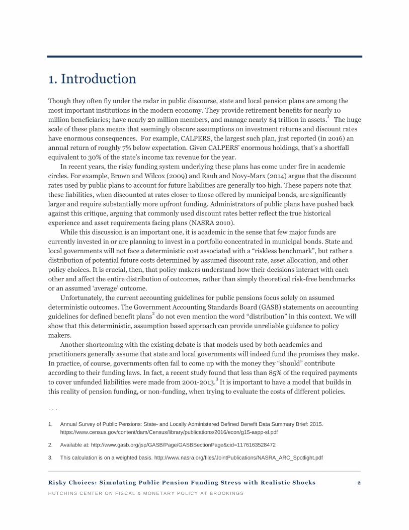
1. Introduction

Though they often fly under the radar in public discourse, state and local pension plans are among the

most important institutions in the modern economy. They provide retirement benefits for nearly 10

million beneficiaries; have nearly 20 million members, and manage nearly $4 trillion in assets.1 The huge

scale of these plans means that seemingly obscure assumptions on investment returns and discount rates

have enormous consequences. For example, CALPERS, the largest such plan, just reported (in 2016) an

annual return of roughly 7% below expectation. Given CALPERS’ enormous holdings, that’s a shortfall

equivalent to 30% of the state’s income tax revenue for the year.

In recent years, the risky funding system underlying these plans has come under fire in academic

circles. For example, Brown and Wilcox (2009) and Rauh and Novy-Marx (2014) argue that the discount

rates used by public plans to account for future liabilities are generally too high. These papers note that

these liabilities, when discounted at rates closer to those offered by municipal bonds, are significantly

larger and require substantially more upfront funding. Administrators of public plans have pushed back

against this critique, arguing that commonly used discount rates better reflect the true historical

experience and asset requirements facing plans (NASRA 2010).

While this discussion is an important one, it is academic in the sense that few major funds are

currently invested in or are planning to invest in a portfolio concentrated in municipal bonds. State and

local governments will not face a deterministic cost associated with a “riskless benchmark”, but rather a

distribution of potential future costs determined by assumed discount rate, asset allocation, and other

policy choices. It is crucial, then, that policy makers understand how their decisions interact with each

other and affect the entire distribution of outcomes, rather than simply theoretical risk-free benchmarks

or an assumed ‘average’ outcome.

Unfortunately, the current accounting guidelines for public pensions focus solely on assumed

deterministic outcomes. The Government Accounting Standards Board (GASB) statements on accounting

guidelines for defined benefit plans2 do not even mention the word “distribution” in this context. We will

show that this deterministic, assumption based approach can provide unreliable guidance to policy

makers.

Another shortcoming with the existing debate is that models used by both academics and

practitioners generally assume that state and local governments will indeed fund the promises they make.

In practice, of course, governments often fail to come up with the money they “should” contribute

according to their funding laws. In fact, a recent study found that less than 85% of the required payments

to cover unfunded liabilities were made from 2001-2013.3 It is important to have a model that builds in

this reality of pension funding, or non-funding, when trying to evaluate the costs of different policies.

. . .

1. Annual Survey of Public Pensions: State- and Locally Administered Defined Benefit Data Summary Brief: 2015.

https://www.census.gov/content/dam/Census/library/publications/2016/econ/g15-aspp-sl.pdf

2. Available at: http://www.gasb.org/jsp/GASB/Page/GASBSectionPage&cid=1176163528472

3. This calculation is on a weighted basis. http://www.nasra.org/files/JointPublications/NASRA_ARC_Spotlight.pdf

https://www.census.gov/content/dam/Census/library/publications/2016/econ/g15-aspp-sl.pdf

http://www.gasb.org/jsp/GASB/Page/GASBSectionPage&cid=1176163528472

http://www.nasra.org/files/JointPublications/NASRA_ARC_Spotlight.pdf

_________________________________________________________________________________________________________



In this paper, we aim to remedy this gap in the discussion. Building on models by Josh McGee and

Michelle Welch (2014a, 2014b) we incorporate a realistic set of asset classes and return shocks into the

model. We allow for plans to invest in a range of different asset classes, and simulate return processes that

build in historical across-class correlations and non-normality. Using data on historical, within-class

performance by public funds, we also estimate time-varying idiosyncratic variances within asset classes.

The size of these idiosyncratic shocks vary with the cycle or average return, and together, create a rich and

realistic distribution of asset market results. We then allow the model to dynamically account for these

shocks, simulate return draws, and track how the system evolves over stochastic iterations. We calibrate

the model to one large system, the Texas Employee Retirement System. By looking at the distribution of

outcomes under different scenarios for this prototypical system, we can better shed light on the impact of

policy choices and economic assumption on outcomes.

This exercise generates a few important insights. The first, and likely most important, is that the

existing status quo is enormously risky. In our baseline simulation for the Texas ERS, under its current

policies, the sum of the discounted amortized payments required over a 30-year period and final

unfunded liabilities has a standard deviation of roughly 7.25% of the total present discounted value of

payroll over that period. This means that the total cost to the taxpayers of Texas will vary significantly

with states of the world going forward. The current system of pension accounting, whatever the discount

rate used, doesn’t convey the risks inherent in the system and how policy choices affect those risks. In our

conclusion, we discuss statistics that public plans could report using these types of simulations to make

this risk transparent to policymakers.

Related to this point, our simulations highlight the risk-reward tradeoff associated with riskier

pension plan allocations. GASB standards implicitly recognize the ‘reward’ side of riskier allocations by

tying discount rates to expected returns, a point also made by Andonov et al (2015). And indeed, our

simulations confirm, that more often than not, these allocations do generate superior results. When

comparing outcomes for the median asset return simulation, shifting assets into riskier categories like

equities generally yields a faster path toward full funding and smaller over all payments en route to that

destination. For example, shifting an additional 15% of the Texas ERS system into equities from money

markets and debt reduced the time until full funding, at the median of the return distribution, by roughly

5 years.

The gains, of course, are not without tradeoffs, and GASB standards do not account for these risks in

any meaningful way. While outcomes are better at the median, performance in the left tail of the return

distribution are dramatically worse. The gap in the 95th percentile of the distribution, between the

baseline allocation and the riskier one mentioned above, is enormous. The riskier allocation winds up

costing roughly 15% more under the Texas ERS calibration, which over 30 years generates a price tag of

over $46 billion in present discounted value costs.

Our simulations also clarify some of the ongoing debate regarding appropriate discount rates.

Changes in the discount rate have a perverse immediate impact on liabilities and funded ratios in that

funds with higher rates and lower contributions appear better funded on impact. Over time, though, the

reduced contributions associated with higher discounting leads to more not less underfunding.

In our simulations, plans that systematically make contributions based on discount rates significantly

below average asset returns usually do wind up fully funded, despite the current risk-inducing allocations.

Of course, it is possible for plans to put away “too much” money too, in the sense that pensions can

become overfunded. Additionally, it is inefficient for plans to make large contributions if asset returns fall

_________________________________________________________________________________________________________



below discount rates. Thus the ‘cost-minimizing’ discount rate4 depends non-linearly on the realization of

investment returns. The wide range of potential outcomes generated by risky asset allocations thus makes

it difficult to plan, which is itself a source of risk.

Finally, our simulations demonstrate that the impact of state and local government meeting their

funding their commitments also depends on a fund’s investment returns. The relationship between the

returns a plan earns and the impact of contributing its payments on funding status and overall costs is

also non-linear. When asset market returns are very strong, failing to make contributions does not really

affect the plans funded status. The larger than expected investment income can replace the shortfall and

ensure the plan is adequately funded. Full initial contributions lead to overfunding in this situation.

Conversely, when asset market returns are weak, early up-front contributions are multiplied by years of

sub-par returns and make a smaller dent in the unfunded liabilities. Our simulations confirm that the

impact of responsibility is largest when returns are in an intermediate range.

Though there is a large literature on public sector pensions, there are only a few papers undertaking

simulation exercises similar to the ones we conduct here. Perhaps most similar is a contemporaneous

paper by Boyd and Yin (2016) that similarly tries to simulate the impact of different funding policies with

an assumed stochastic distribution of returns. Though the details of the model differ, they reach similar

conclusions regarding the degree of risk in the system. Other papers that calculate outcomes for pension

systems under a distribution of outcomes include Rauh and Novy-Marx (JPE 2014), which explores the

impact of linking benefits to returns in a risk sharing environment, and Munnell, Aubry, and Hurwitz

(2013), which tests the sensitivity of funding ratios to investment returns. Maurer, Mitchell, and Rogalla

(2009) simulate pension outcomes for a proposed reform of public sector pensions in Germany, and

CalPERS undertook a simulation exercise designed to measure risk for its members (CalPers 2014).5

The importance of this issue can be seen in municipal pension plans around the country as the threat

of default looms. Understanding the impact of plan decisions on the riskiness of the plan is fundamental

to understanding the value of the benefits to employees and the costs to employers and ultimately

taxpayers. Bottazzi, Jappelli and Padula (2006) and Card and Ransom (2011) find that beneficiaries

adjust their expectations and private wealth accumulation decisions based on pension reforms. With

courts hearing cases (Cloud, 2011) and allowing changes to plan benefits based on the financial state of

the municipality and pension plan in light of the Great Recession, the ability of each economic agent to

understand the distribution of outcomes they face is critical to their own decision making.

Many pensions face a challenge to overcome the benefit enhancements that followed a flush time in

the late 1990s (Koedel, Ni and Podgursky, 2014) that shifted wealth from the recently employed to the

retiring. These enhancements left funds in a position where they may need to reduce/freeze benefits,

increase contributions or investment more aggressively (Rauh 2010).

To address the issues around the impact of contributions, investment allocations and discount rate

selection, this paper proceeds as follows. In the next section, we lay out the math underlying our model

and the unique method we use to generate a plausible distribution of investment returns. In section 3, we

explore the output from our simulation and discuss their implications. Section 4 discusses potential policy

responses to the simulations and concludes.

. . .

4. Note, the cost minimizing rate may not be the same as the rate needed to calculate the market value of the liabilities.

5. https://www.calpers.ca.gov/docs/forms-publications/annual-review-funding-2014.pdf

https://www.calpers.ca.gov/docs/forms-publications/annual-review-funding-2014.pdf

_________________________________________________________________________________________________________



2. Model of Pension Dynamics

To simulate the funded status of pensions it is required that both the expected future liabilities and assets

be calculated. We embed the techniques in McGee and Welch (2014a, 2014b) into a discrete-time dynamic

model wherein each period’s values reflect updates based on stochastic asset returns. Specifically, we have

the two endogenous state variables UL (unfunded liabilities) and MV (the market value of assets) evolve

according to the following laws of motion:

ULt+1 = Lt+1– MVt+1

MVt+1= MVt+ Ct + Rt – Pt

where R represents the total, stochastic return of the plan and P represents payouts accrued by an

exogenous workforce evolution process. The plan’s total contributions, C, is defined by the equation:

Ct = NCt + 𝐶𝑡 = 𝑁𝐶𝑡 + 𝐴𝑡 + 𝑚𝑖𝑛 (𝑀𝑉𝑡, 0)

where NC is the Normal Cost as determined by the exogenous workforce evolution process. The final term

in this equation reflects the fact that the fund must cover any negative asset value immediately. We use

the McGee-Welch algorithm to calculate an updated NC period-by-period.

NCt = NC_Fract * TotalPayrollt

NC_Fract = PVBt/CCWt

where:

TotalPayrollt is the aggregated sum of the salaries of all workers in period t;

PVBt is the expected present value of benefits to all current workers in period t, discounted at the

plan’s selected discount rate;

CCWt is the present value of the expected future salaries to all current workers in period t, discounted

at the plan’s selected discount rate.

The expected future benefits and payroll are a function of plan provided separation and mortality

rates, salary information, a benefit formula and inflation. The benefit formula uses years of service at

separation, retirement age, salary data and a benefit percentage in order to calculate the initial benefit, B.

The model allows for annual cost of living adjustment (COLA) so that B is increased annually by an

assumed COLA.

The pension formula built into the model is based on final average salary defined benefit system (FAS

DB). Workers in an FAS DB system are provided a lifetime annuity based on their final average salary and

years of service, as outlined by McGee and Welch:

B(𝑎𝑟|𝑎𝑠) = 𝑌𝑂𝑆𝑎𝑠∗ 𝑀𝑎𝑟,𝑌𝑂𝑆 ∗ 𝑅𝑎𝑟,𝑌𝑂𝑆 ∗ (1 − 𝐸𝑎𝑟 ,𝑌𝑂𝑆) ∗ 𝐹𝐴𝑆𝑎𝑠

𝐹𝐴𝑆 = 1

𝑦∑ 𝐶𝑊𝑡

𝑎𝑠

𝑡=1+𝑎𝑠−𝑦

where YOS is the years of service, M is the benefit multiplier, R is an indicator of retirement eligibility, E

is a reduction percentage for early retirement, y is the number of years used in the final average salary

calculation and CW is the current wage. The wages for the workers evolve along a pre-set salary vector

which grows with inflation.

_________________________________________________________________________________________________________



The expected present value of benefits to a worker are calculated using standard actuarial techniques

that account for the probabilities of separation and mortality for each age-tenure combination.

In order to account for the common option of the employee withdrawing from the plan and choosing

to take their own contributions along with any vested employer contributions rather than the annuity, the

model calculates the present value of benefits as:

𝑃𝑉𝐵 = 𝑚𝑎𝑥[𝑃𝑉𝐵𝐴𝑛𝑛𝑢𝑖𝑡𝑦 , 𝑓(𝐸𝐸𝐶, 𝐸𝑅𝐶, 𝑟𝑠𝑡𝑎𝑡𝑒𝑑)]

where f is a function that represents a plan’s rules for withdrawing contributions based on the employee

contributions (EEC), employer contributions (ERC) and the stated rate of return on those contributions

(𝑟𝑠𝑡𝑎𝑡𝑒𝑑).

To consider the total benefits that the plan should expect to pay, the model aggregates the present

value of benefits for all current workers. The normal cost in a given period is then calculated as the ratio of

the present value of benefits of the current workers to the present value of payroll of the current workers

multiplied by the current payroll. In order to find the present value of the payroll we need to consider the

evolution of the workforce.

We performed transformations to the current workforce with the assumptions that:

1. The entry age distribution for new hires is constant and equal to the current age distribution

of the workers with one year of service.

2. The workforce will grow at a constant rate and that the number of newly hired workers will be

a function of the growth of the workforce and the separation rates.

To evolve the workforce over time the current workforce was multiplied by one minus the separation

matrix (WFremainingt), aged by 1 year and added to new hires (NewHirest).

Following McGee and Welch, the workforce is described by a k x k upper triangular matrix, W, where

k is equal to the difference between the oldest age possible in the model and the youngest entry age, plus

1. The rows of the matrix represent the entry age of the workers while the columns represent the current

age. The diagonal of the matrix represents the most recently hired workers (their entry age is equal to

their current age). It is the diagonal of the initial workforce that is used to set the age distribution of all

newly hired workers.

The process of removing separating workers requires an element by element multiplication of the

workforce by the k x k separation matrix, as provided by a plan, resulting in W’. Prior to adding the new

workers to W’, the remaining workers must be aged 1 year. This is accomplished by multiplying W’ by a

shift matrix, A, which is a k x k matrix with ones on the super-diagonal, as shown below:

W′ = [

xa0,a0⋯ xa0,ak

⋮ ⋱ ⋮0 ⋯ xak,ak

]

A =

[ 0 1 0 ⋯ 0⋮ 0 1 ⋱ ⋮⋮ ⋮ ⋮ ⋱ ⋮0 0 0 ⋯ 10 0 0 ⋯ 0]

_________________________________________________________________________________________________________



The multiplication of W’ and A will yield W’’, the matrix of remaining workers now one year older,

and thus with one more year of experience.

The process of adding the new workers to the now-aged existing workers requires generating a matrix,

Φ’, which will be added to W’’ to create the complete next period workforce. In order to generate Φ’, we

must first generate Φ, which is a k x k matrix of k columns of the vector of new hires, 𝑛𝑒⃗⃗⃗⃗ , by age. The

vector 𝑛𝑒⃗⃗⃗⃗ is created by multiplying each element of 𝑒 , the distribution of new hires as determined by the

age distribution of first year employees in the initial workforce, by a scaler p, the population of new hires

required to fulfill the required workforce growth. The number of new hires required is found by:

#WFt*(1 + G) = #WFremainingt + #NewHirest

where the #WFt is the number of workers in the workforce at time t, G is the growth rate of the workforce,

#WFremainingt is the number of workers in WFremainingt, and #NewHirest is the number of new hires

required.

This process is continued iteratively to generate the future workforce.

To properly account for the normal cost, only the payroll and benefits of the current workforce is

considered each period. The iterative process then recalculates the PVB and CCW each period based on

the new, current workforce.

The amortization cost, A, is also calculated using methods developed in the McGee and Welch paper.

We depart from that setup, however, in that At+1 is calculated each period as a function of the then current

funding level and payroll rather than as a function of the initial A. Additionally, we allow for the relaxation

of the assumption that the full contribution is made.

At = LevPctt*TotalPayrollt

LevPctt = ULt/CCW30t

where:

CCW30t is the present value of the expected future payroll to all current workers over the following 30

years from period t, discounted at the plan’s selected discount rate.

Here, we have assumed an open 30 year level-percent payoff method for the unfunded liability. In

other words, the required payments are set based on a thirty year amortization horizon that is

recalculated each period. There are alternative methods to amortization payment calculations as well.

Closed, rather than open, methods would preset the amortized payment for future periods, while level-

dollar, rather than level-percent, would fix the dollar payment rather than allow it to float with the size of

the payroll. Boyd and Yin (2016) note that among funds listed in the Public Pension Plans Database a pure

closed method is atypical and either an open or hybrid method are most common. Additionally, over 70%

of funds use a level percent, rather than level dollar method.

CCW30t is found in similar way to CCW, with the exception being that the model only looks forward

to 30 years of payroll rather than the entire possible tenure of the current workforce.

The unfunded liability, UL, of the plan, is the difference between the plan’s liabilities and its assets.

The liability is the present value of future payouts to current plan members (current workers, separated

but not yet retired and retirees) and a function of the benefit formula, discount rate, COLA, wages, wage

growth, workforce, separation and mortality matrices.

While a full history of the prior workers (already separate/retired) would allow for an elegant solution

whereby the model-estimated benefits owed each year could be used to calculate the plan liabilities and

_________________________________________________________________________________________________________



resulting amortized cost, the lack of the complete data offers the options of attempting to estimate and

recreate the prior workforce and rebuild it based on assumptions of prior growth and separations or make

similar assumptions about the growth of liabilities and benefits for all participants together. To simplify

this process, we have assumed that the liabilities and benefit payments increase in proportion to the

growth in payroll over time with the initial levels provided in the plan data. After projecting the workforce

evolution and calculating the total payroll for all workers during each period, the growth in payroll is

calculated. This method allows for an approximation of the impacts due to changes in the workforce

distribution across age and tenure and the resulting impacts on total payroll to be included in the model.

To allow for changes in the assumed discount rate to impact the liabilities and amortized costs we

calculated the Adjusted Liability (AL) by finding the Liability Adjustment Factor (LAF) as:

AL = L * LAF

LAF = 1+ ∑

(1+𝑔)𝑛

(1+𝑏)𝑛𝑇𝑛=1

1+ ∑(1+𝑔)𝑛

(1+𝑎)𝑛𝑇𝑛=1

where T is the liability payoff time, g is the payroll growth rate, b is the new discount rate and a is the

original discount rate (the one used by the plan to calculate the initial liabilities). The method differs from

the one used by McGee and Welch in that they used the ratio of the discount rates compounded out to the

duration of the liabilities. While a practical calculation, the duration of the liabilities was not available in

the plan data and is subject to some variation over time as the distribution of plan participants changes.

Our method gives a similar result numerically and allows for changes over time as the payroll growth rate

varies. It is derived as follows:

L = ∑CFn

(1 + r)n

T

n=0

where 𝐶𝐹𝑛 are the future benefits to be paid to the prior and current workers and r is the plan’s discount

rate.

When considering the future benefits, we made a simplifying assumption that the benefit payouts

would grow along with payroll so that:

𝐶𝐹𝑛 ∗ (1 + 𝑔) = 𝐶𝐹𝑛+1

This would give us the following:

𝐿 = ∑𝐶𝐹0 ∗ (1 + 𝑔)𝑛

(1 + 𝑟)𝑛

𝑇

𝑛=0

𝐿 = 𝐶𝐹0 ∗ (1 + ∑(1 + 𝑔)𝑛

(1 + 𝑟)𝑛

𝑇

𝑛=1)

Adopting the notation of the b as the new discount rate and a as the old discount rate we would have the

following:

𝐿′

𝐿=

𝐶𝐹0 ∗ (1 + ∑(1 + 𝑔)𝑛

(1 + 𝑏)𝑛𝑇𝑛=1 )

𝐶𝐹0 ∗ (1 + ∑(1 + 𝑔)𝑛

(1 + 𝑎)𝑛𝑇𝑛=1 )

_________________________________________________________________________________________________________



where L’ is the new liability.

When considering changes in discount rates our unfunded liabilities would then be calculated as:

ULT+1 = LAFT+1 * LT+1– MVT+1

This model updates iteratively so that each period, the new workforce and asset returns impact the

current assets, liabilities and net cash flows with the assumption that the plan would rebalance to the

target allocation. While the original model used in McGee and Welch set the Amortized Cost as a level

percentage of payroll, allowing for uncertain asset returns and skipping payments requires a recalculation

of the Amortized Cost each year in an open payoff method assumption.

Finally, we must consider the mechanics of the asset levels. The initial asset level is provided by the

plan and the model allows for user inputs for asset allocations. In addition to generating returns, the

assets are also impact by benefit payments and contributions. The normal and amortized contributions to

the plan are calculated within the model and update iteratively as the model evolves through time. While

the model calculates the future benefits of the current workforce, it lacks the year-by-year benefits owed

to the prior workforce. As previously described, the benefit payments are set initially at the plan specified

level and allowed to grow along with payroll each year.

With this model in hand, we now turn to simulating pension dynamics under different parameters.

First, we will address asset allocation across asset classes while allowing for within asset class shocks.

Second, we will address the impact of discount rate selection on the overall cost of the plan and

distribution of results. Finally, we will address the skipping and reducing amortized cost contributions.

3. Simulations

3.1 The Distribution of Returns

One of the key elements of generating realistic simulations for our model is using a realistic distribution of

asset returns. Much of the existing literature has conducted simulations assuming returns are drawn from

standard distributions like a normal or log-normal random variable. Such an approach ignores the

considerable skewness and kurtosis in the actual distribution of returns.

To remedy this, we begin by collecting historical data on annual returns for widely used benchmark

series for eleven different asset classes. Table 1 lists these benchmarks.

Table 1.

Asset Class Benchmark Index

Domestic Equities S&P 500

Fixed Income Barclays Global Bond Index

International Equities MSCI World ex-USA USD

Private Equity Common fund Private Equity

Marketable Alternatives HFRI Fund of Funds

Venture Capital Common fund Capital Venture Capital

Real Estate NCREIF Open-End Diversified Core Energy & Natural Resources S&P Global Natural Resources Commodities DJ-UBS Commodity

Distressed Debt HFRI Distressed Debt

Short-Term Securities/Cash S&P/BGC 0-3m US T-bill TR

_________________________________________________________________________________________________________



To preserve the realistic correlation structure across asset classes, in each period of the simulations,

we draw one year of the historical distribution. The asset class return data is drawn from annual returns

from 1986 – 2013. We then begin our asset return simulation using the return for each benchmark in that

period.

Of course, individual funds experience variation around these benchmarks. Moreover, this variation is

not constant over the business cycle. To model this, we assume that the return earned by any fund is equal

to

𝑅𝑎,𝑖 = 𝑅𝑎,𝑦 + 𝜀𝑎,𝑖,𝑦

where 𝜀𝑎,𝑦 is a draw from a normal distribution with 𝜇 = 0 and 𝜎 = 𝜎𝑎 + 𝛽𝑎𝑅𝑎,𝑦. The mean return 𝑅𝑎,𝑦 is

the return drawn from year y for asset class a, and 𝑅𝑎,𝑖 is the simulated return for asset class a for iteration

i.

To estimate the parameters 𝜎𝑎 and 𝛽𝑎, we collected several years of data on within-asset class returns

for public pension plans in the Pensions & Investments Database. While this series is not long enough to

use for the baseline return draw, it was sufficient to estimate the standard deviation of within-class

returns and the correlation of this standard deviation with the average return. We estimated these

individual plan level shocks for equities, 3-month treasuries, 10-year debt, private equity, real estate and

global debt. For the other classes we experiment with both (1) not assuming individual level shocks and

(2) matching to the individual shocks of other known classes. Since these other classes generally receive

smaller weight in allocation decisions, our results are not sensitive to this decision. The 𝜎𝑎 for each of the

measured asset classes (equities, 3-month treasuries, 10-year debt, private equity, real estate and global

debt) were determined to be 0.06, 0.035, 0.049, 0.1, 0.108 and 0.0 while the 𝛽𝑎 were determined to be -

0.2, 0, -0.2, 0.0, -0.15 and 0.0, respectively. Thus, after drawing a year and average benchmark returns,

we draw individual asset class shocks using these ‘cyclical’ model standard deviations. This allows for the

maintenance of correlation across asset classes, non-normal distribution of returns and within-asset class

variation that is responsive to the size of the return in a given year.

We model our example plan on the Texas Employee Retirement System, a choice we will make

throughout this section. Our TX ERS allocation assigns a weight of 45%, 6%, 15%, 10%, 14% and 10%

distributed across equities, 3-month treasuries, 10-year debt, private equity, real estate, and global debt,

respectively. This allocation assigns zero weight to the other classes, and so those benchmarks are not use

in the simulation. This baseline distribution has a mean of 10.48% and a standard deviation of 9.72%. The

skewness and kurtosis of the distribution are -.8 and 4.26, which indicates heavy tails and is in line with

findings from the literature (Egan 2007).

While we allow for a rich correlation structure in returns within-year across asset classes, we assume

independent draws from the data generating process across years. The distribution of annualized returns

over a twenty-five-year period has a smaller variance than the annual return. The median annualized

return under the base distribution is 11.7% (with a standard deviation of 2.1%). Though this variance

might appear minor, the heterogeneity in possible outcomes results in large differences in fiscal costs. If

applied to the starting asset value, the difference between the 75th percentile and 25th percentile of this

range is 1060% of the initial asset value.

Is this large standard deviation reasonable? Using data from Shoag (2011) and Farrell and Shoag

(2012) on pension returns from the 1980s onward, we find the standard deviation of annualized

cumulative twenty-five year returns is roughly 0.67%. That’s the variation across plans within one

_________________________________________________________________________________________________________



realization of the world. The Boston College PPD similarly has an unweighted standard deviation of

annualized returns from 2001-2015 of 0.87%. Given the large idiosyncratic variation within a given set of

aggregate returns, a number like 2.1% across possible realizations of the world of aggregate returns seems

credible.

A crucial fact to note is that mean return generated by this simulation process is large and exceeds

both the discount rate used by the Texas ERS and the long run average return reported in Shoag (2011).

The long run average in that paper may not be a useful benchmark, however, given the greater weight

placed on riskier, higher return assets over time.

Our distribution also has a higher mean return than the average annual return reported from 2001-

2015 in the Boston College Public Plan Database. That data set has a weighted mean return of 6.7% and a

weighted median of 9.8%. One reason for this large difference is that this has been a relatively atypical

period, historically, in terms of asset market returns. The distribution of index returns includes years with

high returns outside this recent window. When excluding the “Great Recession” from this dataset our

simulated distribution better fits the data. The mean and median weighted returns in the PPD excluding

the recession are 10.1% and 11.8% respectively, relative again, to our simulated mean of 10.4%.6

We plot the CDF of returns of returns from the Boston College Public Plans data and our simulations

below. As can be seen in the graph, the two distributions are largely similar, only our simulations are

centered on a higher mean.

Figure 1.

It is difficult to overstate just how important this gap is for the likely evolution of plan dynamics. In

Figure 2 below we plot the evolution of the amortization and shortfall costs as a percentage of payrolls

. . .

6. The PPD shows a similar pattern for the Texas ERS, which has an average return of 5.6% over the period and 10.6% when

excluding the recession.

_________________________________________________________________________________________________________



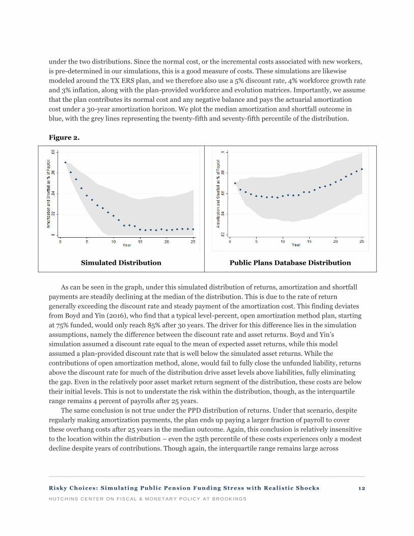
under the two distributions. Since the normal cost, or the incremental costs associated with new workers,

is pre-determined in our simulations, this is a good measure of costs. These simulations are likewise

modeled around the TX ERS plan, and we therefore also use a 5% discount rate, 4% workforce growth rate

and 3% inflation, along with the plan-provided workforce and evolution matrices. Importantly, we assume

that the plan contributes its normal cost and any negative balance and pays the actuarial amortization

cost under a 30-year amortization horizon. We plot the median amortization and shortfall outcome in

blue, with the grey lines representing the twenty-fifth and seventy-fifth percentile of the distribution.

Figure 2.

Simulated Distribution Public Plans Database Distribution

As can be seen in the graph, under this simulated distribution of returns, amortization and shortfall

payments are steadily declining at the median of the distribution. This is due to the rate of return

generally exceeding the discount rate and steady payment of the amortization cost. This finding deviates

from Boyd and Yin (2016), who find that a typical level-percent, open amortization method plan, starting

at 75% funded, would only reach 85% after 30 years. The driver for this difference lies in the simulation

assumptions, namely the difference between the discount rate and asset returns. Boyd and Yin’s

simulation assumed a discount rate equal to the mean of expected asset returns, while this model

assumed a plan-provided discount rate that is well below the simulated asset returns. While the

contributions of open amortization method, alone, would fail to fully close the unfunded liability, returns

above the discount rate for much of the distribution drive asset levels above liabilities, fully eliminating

the gap. Even in the relatively poor asset market return segment of the distribution, these costs are below

their initial levels. This is not to understate the risk within the distribution, though, as the interquartile

range remains 4 percent of payrolls after 25 years.

The same conclusion is not true under the PPD distribution of returns. Under that scenario, despite

regularly making amortization payments, the plan ends up paying a larger fraction of payroll to cover

these overhang costs after 25 years in the median outcome. Again, this conclusion is relatively insensitive

to the location within the distribution – even the 25th percentile of these costs experiences only a modest

decline despite years of contributions. Though again, the interquartile range remains large across

_________________________________________________________________________________________________________



realization within this distribution, at 4% of payrolls. In total, these comparisons highlight how big an

impact the shift in the return distribution will have on these outcomes.

Of course, the distribution of amortization costs is only one measure of plan financial health, and a

spot measure at that. It does not factor into account extant unfunded liabilities. Similarly, considering

only unfunded liabilities would ignore prior differences in amortization payments. To more broadly

consider the impact of the PPD versus the simulated return distribution, we measure the present

discounted value of all prior amortization and shortfall payments along with any remaining unfunded

liabilities after thirty years, divided by the present discounted value of all past payroll. We plot the

distribution for both the PPD and simulated asset distributions in Figure 3 below.

Figure 3.

As can be seen in the figure, the simulated distribution has far smaller total costs. At the mean, these

differences are 14.6% of the total PDV of payroll over the period. Needless to say, this represents an

enormous difference in fiscal costs, and one that would be difficult for state and local governments to

cover. Of course, even within the distributions themselves there is enormous risk. The interquartile range

in the simulation and PPD data is almost as large as the gap between the two distributions themselves:

11.7% and 9.1% of payroll respectively. The net result shows just how risky – or wide a variety of outcomes

– are possible under the current system. Both across and within distributions, the potential range of

funding requirements is enormous relative to current values and state budgets.

Going forward, we will use the simulated distribution of returns to consider the impact of changing

asset allocations (which is not possible with the PPD approach), discount rates, and payment failures.

While we have attempted to create a realistic model, it is important to keep in mind that – if anything –

we are using a generous distribution of returns. It is impossible to know if the next thirty years will look

like the 1980s and 1990s or the last fifteen years in terms of aggregate market performance. This is

obviously not a choice variable for policymakers. The risks we will consider going forward are all

measured for choices within a distribution of returns, but the center of the distribution is obviously itself a

huge risk with large implications as shown above.

_________________________________________________________________________________________________________



3.2 Baseline and the Impact of Asset Allocation

In the previous section, we highlighted the importance of large returns in determining total fiscal cost for

a pension fund. In this section we consider perhaps the most intuitive determinant of returns, asset

allocation. If the fiscal future of public funds is so tied to high returns, what is the consequence to shifting

assets to investments that historically have offered greater returns?

We test this by consider two asset allocations within our simulated return frame work, a relatively

risky one with a weight of 66%, 0%, 0%, 10%, 14% and 10% distributed across equities, 3-month

treasuries, 10-year debt, private equity, real estate, and global debt and a more conservative, and our base

case allocation with a distribution of 45%, 06%, 15%, 10%, 14% and 10% across the same. The more

conservative allocation is, again, an approximation of the current Texas ERS asset allocations. The riskier

allocation is loosely based on the allocation advanced in the Government Accounting Standards Board

2012 statement on financial reporting for public pension plans.7

The impact on the cumulative distribution function of annual returns is presented in Figure 4 below:

Figure 4.

Again, the baseline distribution has a mean of 10.48% and a standard deviation of 9.72%. The

skewness and kurtosis of the distribution are -.8 and 4.26, which indicates heavy tails and is in line with

findings from the literature (Egan 2007). The more aggressive distribution has a mean of 11.74% and a

standard deviation of 13.38%. The skewness and kurtosis are similarly magnified, at -1.15 and 4.93.

Whereas the PPD and simulated return distribution represented a centering shift with relatively little

change in shape, here the relatively risky distribution has a twisting effect on the cumulative distribution

of returns.

. . .

7. P.77

_________________________________________________________________________________________________________



The median annualized return under the risky distribution is 12.7% (with a standard deviation of

3.2%), and the median annualized return under the base distribution is 11.7% (with a standard deviation

of 2.1%).

Though these twenty five-year annualized return differences may appear minor, they have enormous

implications for the financial situation in the plan. The roughly 1% differential at the median, when

compounded, results in a difference equal to four times the asset holdings of the plan. Given that holdings

for a plan like the Texas ERS are roughly 46% of annual tax revenue, this is a very large swing. While the

riskier distribution has more favorable outcomes at the median, the larger variance in annualized returns

is similarly magnified when considering the cumulative impact. The interquartile gap for the riskier

distribution is roughly 21 times the starting asset value, as opposed to the aforementioned already large

interquartile range of 10.6 for the base scenario. Again, given the large base to which these ranges apply,

these shocks imply enormous swings in funding pressure.

To better understand the financial impact, we begin by exploring required payments into the system.

Again, since the normal cost, or the incremental costs associated with new workers, is pre-determined in

our simulations, we track the evolution of the amortization cost and shortfall under the two allocations as

a percent of payroll (also exogenous). Again, we plot the median outcome in blue, with the grey lines

representing the twenty-fifth and seventy-fifth percentile of the distribution.

Figure 5.

Base Allocation Risky Allocation

As is evident in the figures, in the median situation, regularly contributing the ARC mostly eliminates

the amortization costs in twenty to twenty-five years. Again, this is assuming a discount rate of 5% and an

open ended amortization horizon of 30 years. It takes slightly longer and persists at a slightly higher level

under the more conservative allocation, which yields lower returns at the median. In the fortunate, 25th

percentile scenarios, these costs are eliminated in less than 10 years under the base allocation. In these

same fortunate scenarios, these costs are eliminated in little over 5 years in the riskier ones.

In the less fortunate case, however, that exists at the 75th percentile of the distribution the

amortization costs remain significant despite these regular contributions. In fact, the riskier distribution

has higher cost for many years at this part of the distribution, despite better outcomes at the median.

_________________________________________________________________________________________________________



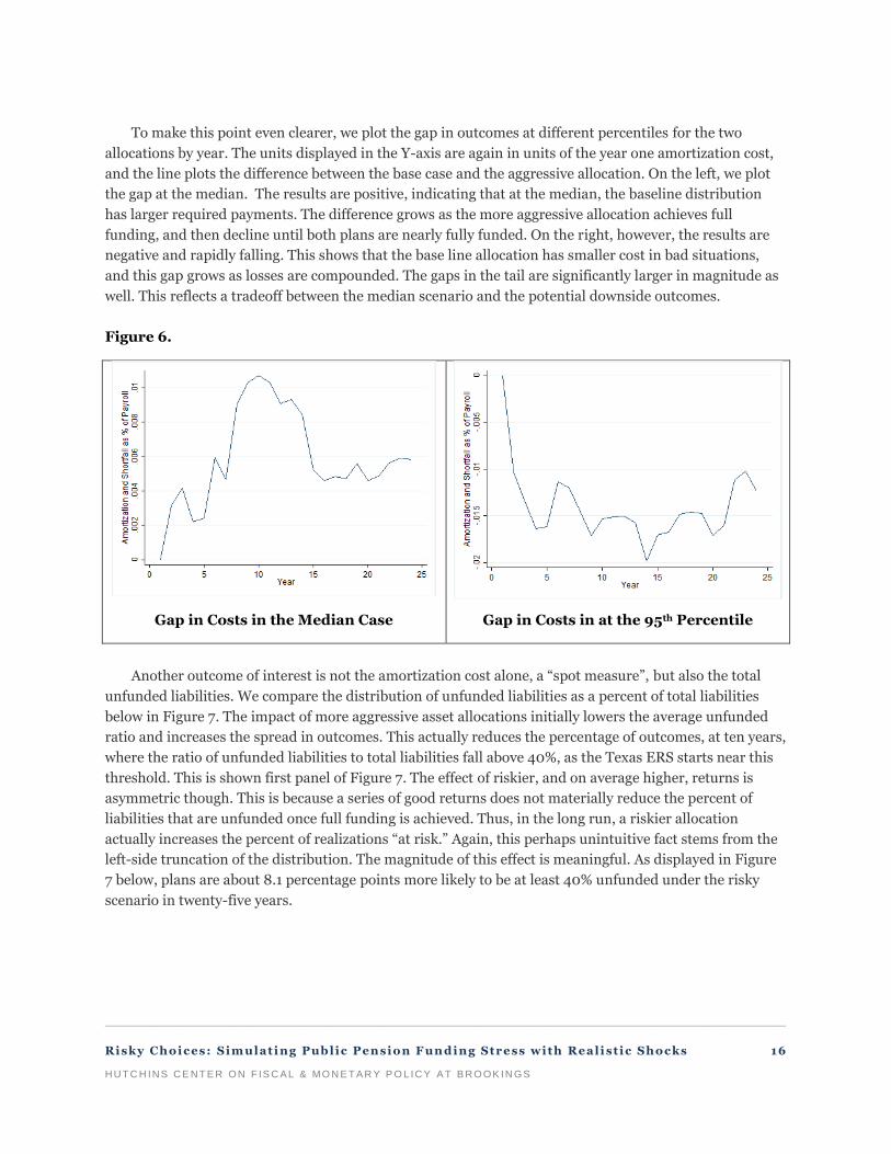
To make this point even clearer, we plot the gap in outcomes at different percentiles for the two

allocations by year. The units displayed in the Y-axis are again in units of the year one amortization cost,

and the line plots the difference between the base case and the aggressive allocation. On the left, we plot

the gap at the median. The results are positive, indicating that at the median, the baseline distribution

has larger required payments. The difference grows as the more aggressive allocation achieves full

funding, and then decline until both plans are nearly fully funded. On the right, however, the results are

negative and rapidly falling. This shows that the base line allocation has smaller cost in bad situations,

and this gap grows as losses are compounded. The gaps in the tail are significantly larger in magnitude as

well. This reflects a tradeoff between the median scenario and the potential downside outcomes.

Figure 6.

Gap in Costs in the Median Case Gap in Costs in at the 95th Percentile

Another outcome of interest is not the amortization cost alone, a “spot measure”, but also the total

unfunded liabilities. We compare the distribution of unfunded liabilities as a percent of total liabilities

below in Figure 7. The impact of more aggressive asset allocations initially lowers the average unfunded

ratio and increases the spread in outcomes. This actually reduces the percentage of outcomes, at ten years,

where the ratio of unfunded liabilities to total liabilities fall above 40%, as the Texas ERS starts near this

threshold. This is shown first panel of Figure 7. The effect of riskier, and on average higher, returns is

asymmetric though. This is because a series of good returns does not materially reduce the percent of

liabilities that are unfunded once full funding is achieved. Thus, in the long run, a riskier allocation

actually increases the percent of realizations “at risk.” Again, this perhaps unintuitive fact stems from the

left-side truncation of the distribution. The magnitude of this effect is meaningful. As displayed in Figure

7 below, plans are about 8.1 percentage points more likely to be at least 40% unfunded under the risky

scenario in twenty-five years.

_________________________________________________________________________________________________________



Figure 7.

Ten Year Status

Thirty Year Status

Base Distribution Risky Distribution

Of course, these funding ratios do not account for differences in payments over the years, which can

be large as demonstrated in Figure 6. Again, we construct a more comprehensive measure by taking the

present-discounted value of amortization and shortfall payments plus any unfunded liabilities as a

fraction of the present-discounted value of total payroll. The safer distribution is significantly less likely to

wind up with very low costs. It is also less likely to wind up in the right tail of this distribution showing

that it limits some of the worse possible outcomes. This effect, evident after 30 years in Figure 8 below.

_________________________________________________________________________________________________________



Figure 8.

The overall picture, then, across several measures is fairly consistent. The system contains a

significant amount of risk given current allocations. Asset markets are quite variable, and even under a

generously modeled distribution, the historical data on plan returns and realistic assumptions imply that

the range of outcomes facing funding governments in enormous. Median outcomes imply a plan like the

Texas ERS is moving towards full funding, but this is not true under many realizations. Even if the Texas

ERS continues to make their full required contributions, and we use the simulated return distribution

with high baseline returns, there is still a greater than 1 in 3 chance that required amortization payments

will be more than 50% bigger in thirty years in absolute terms.

There has been a pronounced trend toward more aggressive allocations by public pensions (Pew

Charitable Trust, 2014). While riskier allocations may reduce costs at median or better returns, they

increase the risk of large payments at the other end of the distribution. This is reflected in both the total

amount paid, annual costs, and funding ratios. Riskier allocations also increase the likelihood of severe

underfunding in both the long and short run. In the longer run, in our simulations, the combined effect of

high compounded asset returns, low discount rates, and regular amortization payments ensures plans

become fully funded under most realizations. This highlights the advantage – in addition to the

importance of asset returns –of regularly meeting the amortization cost and choosing a conservative

discount rate, topics we explore in the next subsection.8 Still, there is a tail of significant risk under more

aggressive allocation even with conservative funding policy.

This discussion also hints at the limitations of existing accounting measures to convey an accurate

sense of the consequences of asset allocation decisions. Neither funding ratios nor amortization costs

provide policymakers with a sense of the impact of these decisions on the distribution of possible

. . .

8. For example, we simulated the base case scenario in which plans only make ½ of their required amortization payment each

year. Though the payment increases as a result, this policy change increases the fraction of plans with more than 40%

unfunded liabilities by more than 50%.

_________________________________________________________________________________________________________



outcomes. A number of the measures we discussed here – say funding ratios at certain moments of the

distribution – do convey that intuition for a given set of accounting assumptions. As we will see below,

these measures are unfortunately sensitive to changes in those assumptions.

3.3 Different Discount Rates

One parameter that has received significant attention in the literature on pension funding is the discount

rate. Many plans set discount rates in line with expected asset returns. Critics charge that the discount

rate should instead reflect the riskiness of the liabilities, which given their state backing, carry risks more

in line with either risk free or municipal bond rates.

Our model allows us to explore the impact of different discount rates on the funding status of the

plan. Our simulations in the previous section proceeded under the conservative (relative to the majority of

plans) discount rate of 5%. To explore the impact of changing this assumption, we simulate plans using

funding rules that follow a 7% discount rate.

On impact, the increase in the discount rate reduces the assumed liabilities considerably. As a result,

the initial funding ratio improves. This can be seen in the rightward shift in the funding distribution at

five years.

Over time, though, this accounting “improvement” in funding ratios does not—in fact—produce

higher investment returns. Despite this, due to the perceived improvement in funding ratios, plans

contribute smaller amounts to deal with future liabilities. As a result of the smaller contribution, funding

ratios begin to fall relative to the distribution without a discount rate change. The distributions become

relatively similar at 15 years, and the entire distribution is shifted left after twenty-five years.

Figure 9.

5 Years 15 Years

_________________________________________________________________________________________________________



25 Years

Of course, the initial “improvement” in funding ratios was an accounting result, not an economic one.

To separate out the impact of the discounting itself from the planning aspects, we compare the khaki

distribution (discounting at 5% but having planned assuming 7%) to a distribution that used 5% for both

discounting and planning. To do this, we use the liability adjustment factor (LAF) previously calculated.

The resulting distributions at 5, 15, and 25 years are plotted in Figure 10 below.

This figure highlights a critical feature of the impact of changing the discount rate. Though moving

the discount rate itself has an impact on funding status, as seen in Figure 9, the more important

consequence of moving the rate is the real impact it has on contributions. Here, when liabilities are

ultimately discounted using the same rate, having set contributions using the higher rate led to 32.6 pp

more plans falling below the 80% asset to constant-discount-rate-measured liabilities at 15 years and 39.2

pp fewer plans below the threshold at 25 years. Again, these results highlight the impact of discounting on

funding outcomes beyond their immediate accounting effect.

Figure 10.

5 Years 15 Years

_________________________________________________________________________________________________________



25 Years

While lower discount rates improve funding ratios, they also require funds to have larger

contributions. There are two potential hazards associated with this requirement. The first is, in the event

of returns below the discount rate, funds are “cheaper” in present discounted value terms the smaller the

historical contributions. For example, had employers ceased contributing immediately before the market

downturn in 2008, they would have saved a considerable amount of money.

The second occurs in the event of good returns. In our model excess assets over and above the

actuarial requirement do not reduce the contributions mandated on employers9. For example, a series of

good returns in Illinois in the 1990s led to more generous pensions offered to system members rather

than savings to the taxpayer (Fitzpatrick 2012). This is also consistent with a long literature on the

“flypaper” effect (see Hines and Thaler 1995) and the findings in Shoag (2011) that gains are not

symmetrically rebated to taxpayers. Thus, if returns are large enough, employers could contribute “too

much” under low discount rates and wind up overfunded. Of course, in the intermediate return range,

large contributions reduce total costs since they exploit favorable returns but do not overfund.

To see this, we once again use our measure of the present-discounted value of amortization and

shortfall payments and the unfunded liabilities at 30 years. We again divide this measure by the present

discounted value of total payroll. We plot this total cost measure against the annualized 30-year return

earned in each simulation. We plot these charts separately for a 5% discount rate (blue) and a 7% discount

rate (red). To keep things comparable, we use 5% as the rate for doing the present discounted value

calculations, even when the plan operated under the 7% discount rate.

. . .

9. Some funding formulas may allow for a reduction in normal contributions if the fund reaches a particular threshold above

100%. Here we work under the assumption that this is not the case.

_________________________________________________________________________________________________________



Figure 11.

The figure confirms the intuition explained above. Under the low return case (less than 5%), the high

discount rate mechanics are cheaper in constant PDV terms. Similarly, to the right of the graph, when

returns are very high, the low upfront contributions from a high discount rate are again cheaper in PDV

terms. In the bulk of the simulations, in the center of the returns distributions, however, things are

cheaper with lower discount rates and high returns. In other words, the investment of increased

amortized contributions driven by initially having a lower discount rate does not pay off when returns are

either much lower or much higher than expected. This difficulty in determining the cost-minimizing

discount rate is another consequence of risky allocations.

Discussions on the appropriate discount rate are often discussed in the literature, but frequent

changes are less common. This non-linear impact of payments also shows up in the more common

practice of plans skip or reduce their amortize cost contributions. The next section evaluates the impact of

such decisions and finds that they are similarly impacted by investment risk.

3.4 Failure to Pay Amortization Cost

In this section, we consider the impact of failing to pay the amortization cost on outcomes. To do this, we

simulate the model with the plan contributing only the normal cost for the first three periods. The time

series evolution of this model is displayed in Figure 12.

_________________________________________________________________________________________________________



Figure 12.

Obviously failing to make payments increases the time it takes plans, at the median, to achieve

effectively full funding. In fact, the median outcome never quite achieves full funding in the twenty-five-

year horizon plotted above. Still, most of the gap in funding can be overcome for much of the distribution

because (1) contributions increase after the three-year break in response to higher liabilities and (2) in our

simulations asset returns outstrip the discount rate in general.

It is important to consider that the impact of failing to make payments may interact with the

stochastic nature of returns, a possibility noted by Boyd and Yin (2016) as well. To explore this, we

consider how annual payments evolve at different parts of the simulated distribution. The impact at the

25th, median, and 95th percentile is presented in Figure 13 below. Unlike Boyd and Yin (2016) and

perhaps counter intuitively, we find a non-linear interaction. The impact of underfunding matters most in

the face of mid-level asset returns.

To see this intuition, note that when asset returns are poor, as in the 95th percentile, the failure to pay

the initial amortization amounts has a small impact relative to the losses in the asset markets. Moreover,

even the payments themselves would have experienced poor returns had they been contributed, and so

their direct contribution would have been smaller.

When returns are very good, say as in the 25th percentile of the distribution, amortization costs tend

towards zero very quickly. While the dollar values lost by failing to make the contributions are large, the

rapid transition to full funding with and without these contributions puts a limit on the reduction in

amortization costs.

The impact of skipping payments, then, is largest when returns are in the middle of the distribution,

as at the median. In this scenario, plans do not immediately achieve full funding, and the gains from the

increased contributions are not wiped out in the asset markets.

_________________________________________________________________________________________________________



Figure 13.

_________________________________________________________________________________________________________



As the previous figure demonstrates, the reduction in contributions depends on the realized returns.

For example, the total reduction in contributions is bigger at the 25th percentile than they do at the

median. Of course amortization costs are not the only aspect of pension accounting impacted by

neglecting to meet required contributions. Lower contributions may translate into lower funding ratios.

To get the full impact, we once again turn to our PDV measure. Like before, we plot the PDV of costs and

unfunded liabilities against annualized return for the two scenarios below:

Figure 14.

Again, skipping payments increases costs at the mean and median of the distribution, but actually

decreases them in the tails. The non-linearity induced by asset market risk makes the consequences of

funding decisions difficult to foresee. As with our analysis of discount rates, risky investments not only

carry risks themselves, but make the appropriate policy decisions more complicated as well.

4. Conclusions and Policy Implications

Our findings are several. First and foremost, our simulations highlight the enormous range of potential

outcomes facing state and local governments. The mean of the return distribution is certainly vital for

determining whether plans are likely to trend towards or away from full funding. Still, across all of the

realistic distributions, whatever their mean, the variation across draws is tremendous. State and local

pension plans manage such large sums that these present substantive risk to their total budgets. Given

that many state and local governments already face many institutional constraints to smoothing revenue

shocks, the uncertainty generated by these funds makes planning difficult.

Second, the movement towards riskier asset classes that has occurred has had a predictable effect on

the distribution of outcomes. While higher risk, higher return allocation improves funding outcomes and

reduces total costs at the median, it also greatly increases costs at the tail of the distribution. Existing

accounting practices, which sometimes do acknowledge the higher expected return associated with riskier

_________________________________________________________________________________________________________



allocations, do not measure or report the accompanying increases in risk. This skews the information and

incentives for policy makers.

Third, funds that switch to a higher discount rate perversely look better funded immediately after the

switch and have lower up front amortized cost contributions. These lower payments combined with asset

returns that underperform relative to the increased discount rate eventually lead to lower funding ratios,

however. The impact of selecting a higher or lower discount rate on total cost is complicated by the wide

range of possible asset returns. The effect here is non-linear, as the total cost of the plan over 25 years are

higher with high discount rates when asset returns are near the mean, but decreases for returns at either

tail.

Fourth, skipping payments has a similar impact to increasing your discount rate in that they lower

your upfront contributions. When returns are near the median, failing to capitalize on these good returns

increases the total cost of the plan over 25 years. If the returns are subpar, or if they are so good as to lead

to overfunding, the total cost decreases with smaller upfront payments.

A final implication of these exercises is that many of the intuitive risk measures discussed in the

Section III (such as funding ratios or amortization payments at a moment of the distribution) are sensitive

to accounting assumptions like the discount rate, asset smoothing period, and amortization horizon. As

such, these risk measures cannot be used to evaluate the impact of these assumptions themselves on the

distribution of outcomes, nor can they be used to evaluate riskiness across plans with different

assumptions. A risk measure that could be used in this way would need to use a constant set of

assumptions, for example a universal fixed discount rate. Having a set baseline for plan to compare

themselves against would allow for greater transparency on plan status and risk.

This should be less contentious than it first appears. As discussed above, there is a long standing and

fierce debate about the appropriateness of linking assumptions like the discount rate to plan specific

features like the asset allocation. Whatever the rationale for making these linkages for funding purposes,

these arguments do not apply in a risk measurement context. Finally, the lack of any existing risk metric is

a clear hindrance to policymakers. The existing reporting by public funds in no way conveys the wide

range of possible funding outcomes. Existing accounting practices often recognize the impact of decisions

on one part of the distribution of outcomes (say the mean or median) without indicating that they also

affect other moments. Simulations based on the model we developed and those similar to it can help

better convey the full impact of policy decisions. We believe that these types of simulations should become

part of the standard public fund reporting.

_________________________________________________________________________________________________________



REFERENCES

Boyd, Daniel and Yimeng Yin. “Public Pension Funding Practices How These Practices Can Lead to Significant Underfunding or

Significant Contribution Increases When Plans Invest in Risky Assets”, Working Paper (June 2016)

Bottazzi, Renata, Tullio Jappelli and Mario Padula. “Retirement expectations, pension reforms, and their impact on private wealth

accumulation.” Journal of Public Economics 90.12 (2006): 2187 – 2212.

Brown, Jeffrey R., and David W. Wilcox. "Discounting state and local pension liabilities." The American Economic Review 99.2

(2009): 538-542.

CalPERS, “Annual Review of Funding Levels and Risks”, November 18, 2014

Card, David, and Michael Ransom. "Pension plan characteristics and framing effects in employee savings behavior." The Review of

Economics and Statistics 93.1 (2011): 228-243.

Cloud, Whitney. "State Pension Deficits, the Recession, and a Modern View of the Contracts Clause." Yale Law Journal 120 (2011):

2199.

Egan, William J. "The distribution of S&P 500 index returns." Available at SSRN 955639 (2007).

Farrell, James, and Daniel Shoag. "Asset management in public DB and non-DB Pension Plans." Journal of Pension Economics and

Finance 15.4 (2016): 379-406.

Fitzpatrick, Maria D. "How Much Do Public School Teachers Value Their Retirement Benefits?" Stanford Institute for Economic

Research Working Paper (2012).

Governmental Accounting Standards Board. 2012. “Financial Reporting for Pensions Plans, an amendment of GASB Statement No.

25.”

Governmental Accounting Standards Board. 2012. “Accounting and Financial Reporting for Pensions, an amendment of GASB

Statement No. 27.”

Hines, James R., and Richard H. Thaler."Anomalies: The flypaper effect”, The Journal of Economic Perspectives 9.4 (1995): 217-

226.

Koedel, Cory, Shawn Ni, and Michael Podgursky. "Who Benefits from Pension Enhancements?" Education 9.2 (2014): 165-192.

Maurer, Raimond, Olivia S. Mitchell, and Ralph Rogalla."Reforming German civil servant pensions: Funding policy, investment

strategy, and intertemporal risk budgeting." (2008).

McGee, Joshua and Michelle Welch. “Modeling Pension Benefits.” 2014 Draft (2014a)

McGee, Joshua and Michelle Welch. “Modeling Pension Costs.” 2014 Draft (2014b)

Munnell, Alicia H., Jean-Pierre Aubry, and Josh Hurwitz. "How sensitive is public pension funding to investment returns." State

and Local Pension Plans (2013).

National Association of State Retirement Administrators. “Faulty Analysis is Unhelpful to State and Local Pension Sustainability

Efforts.” October 2010.

Novy-Marx, Robert, and Joshua Rauh. “The revenue demands of public employee pension promises." American Economic Journal:

Economic Policy 6.1 (2014): 193-229.

Novy-Marx, Robert, and Joshua D. Rauh. "Linking benefits to investment performance in US public pension systems." Journal of

Public Economics116 (2014): 47-61.

Pew Charitable Trusts and the Laura and John Arnold Foundation. “State Public Pension Investments Shift over Past 30 Years.”

(2014)

Rauh, Joshua D. "Are state public pensions sustainable? Why the federal government should worry about state pension liabilities."

National Tax Journal 63.3 (2010): 585-602

Shoag, Daniel. "The impact of government spending shocks: Evidence on the multiplier from state pension plan returns." working

paper, Harvard University (2011).

The mission of the Hutchins Center on Fiscal and Monetary Policy is to improve the quality and efficacy of fiscal and monetary policies and public understanding of them.

Questions about the research? Email [email protected]. Be sure to include the title of this paper in your inquiry.

© 2017 The Brookings Institution | 1775 Massachusetts Ave., NW, Washington, DC 20036 | 202.797.6000

Documents

Risky Choices: Simulating Public Pension Funding Stress