Risk/Arbitrage Strategies: A New Concept for Asset/Liability Management, Optimal Fund Design and Optimal Portfolio Selection

in a Dynamic, Continuous-Time Framework Part IV: An Impulse Control Approach to Limited Risk Arbitrage

Hans-Fredo List Swiss Reinsurance Company

Mythenquai 50/60, CH-8022 Zurich Telephone: +41 1 285 2351 Facsimile: +411285 4179

Mark H.A. Davis Tokyo-Mitsubishi International plc 6 Broadgate, London EC2M 2AA

Telephone: +44 171 577 2714 Facsimile: +44 171 577 2888

Abstract. Asset/Liability management, optimal fund design and optimal portfolio selection have been key issues of interest to the (re)insurance and investment banking communities, respectively, for some years - especially in the design of advanced risk- transfer solutions for clients in the Fortune 500 group of companies. The new concept of limited risk arbitrage investment management in a diffusion type securities and derivatives market introduced in our papers Risk/Arbitrage Strategies: A New Concept for Asset/Liability Management, Optimal Fund Design and Optimal Portfolio Selection in a Dynamic, Continuous-Time Framework Part I: Securities Markets and Part II: Securities and Derivatives Markets, AFIR 1997, Vol. II, p. 543, is immediately applicable to ALM, optimal fund design and portfolio selection problems in the investment banking and life insurance areas. However, in order to adequately model the (RCLL) risk portfolio dynamics of a large, internationally operating (re)insurer with considerable (“catastrophic”) non-life exposures, significant model extensions are necessary (see also the paper Baseline for Exchange Rate - Risks of an International Reinsurer, AFIR 1996, Vol. I, p. 395). To this end, we examine here an alternative risk/arbitrage investment management methodology in which given an arbitrary trading or portfolio management policy the limited risk arbitrage objectives are periodically enforced by (impulsive) corrective actions at a certain cost. The mathematical framework used is that related to the optimal singular control of Markov

jump diffusion processes in Rn with dynamic programming and continuous-time martingale representation techniques.

Key Words and Phrases. Risk/Arbitrage tolerance band, risk exposure control costs, impulsive risk exposure control strategies.

343

Contents (all five parts of the publication series).

Part I: Securities Markets (separate paper) 1. Introduction 2. Securities Markets, Trading and Portfolio Management

- Complete Securities Markets - Bond Markets - Stock Markets - Trading Strategies - Arrow-Debreu Prices - Admissibility - Utility Functions - Liability Funding - Asset Allocation - General Investment Management - Incomplete Securities Markets - Securities Market Completions - Maximum Principle - Convex Duality - Markovian Characterization

3. Contingent Claims and Hedging Strategies - Hedging Strategies - Mean Self-Financing Replication - Partial Replication - American Options - Market Completion With Options

Appendix: References

Part II: Securities and Derivatives Markets (separate paper) 4. Derivatives Risk Exposure Assessment and Control

- Market Completion With Options - Limited Risk Arbitrage - Complete Securities Markets - Options Portfolio Characteristics - Hedging With Options

5. Risk/Arbitrage Strategies - Limited Risk Arbitrage Investment Management - Strategy Space Transformation - Market Parametrization - Unconstrained Solutions

- Maximum Principle - Convex Duality - Markovian Characterization

344

- Risk/Arbitrage Strategies - Dynamic Programming - Drawdown Control - Partial Observation

Appendix: References

Part III: A Risk/Arbitrage Pricing Theory (separate paper) 1. Introduction 2. Arbitrage Pricing Theory (APT)

- Dynamically Complete Market - Incomplete Market

3. Risk/Arbitrage Pricing Theory (R/APT) - General Contingent Claims - Optimal Financial Instruments - LRA Market Indices - Utility-Based Hedging - Contingent Claim Replication - Partial Replication Strategies - Viscosity Solutions - Finite Difference Approximation

Appendix: References

Part IV: An Impulse Control Approach to Limited Risk Arbitrage 1. Introduction 2. Dynamic Programming

- Risk/Arbitrage Controls - Viscosity Solutions - Finite Difference Approximation

3. Impulse Control Approach - Jump Diffusion State Variables - Singular Controls - Markov Chain Approximation

Appendix: References

4 6 6 8 10 12 12 13 15 23

Part V: A Guide to Efficient Numerical Implementations (separate paper) 1. Introduction 2. Markovian Weak Approximation 3. An Example: Implied Trees 4. Diffusion Parameter Estimation 5. Securitization Appendix: References

345

1. Introduction

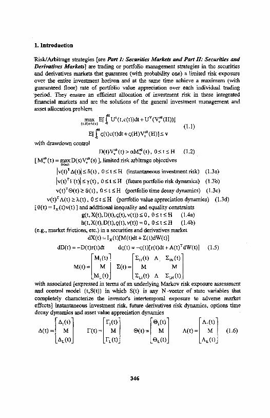
‘Risk/Arbitrage strategies (see Part I: Securities Markets and Part II: Securities and Derivatives Markets] are trading or portfolio management strategies in the securities and derivatives markets that guarantee (with probability one) a limited risk exposure over the entire investment horizon and at the same time achieve a maximum (with guaranteed floor) rate of portfolio value appreciation over each individual trading period. They ensure an efficient allocation of investment risk in these integrated financial markets and are the solutions of the general investment management and asset allocation problem

with drawdown control

limited risk arbitrage objectives

(instantaneous investment risk) (1.3a)

(future portfolio risk dynamics) (1.3b)

(portfolio time decay dynamics) (1.3c)

(portfolio value appreciation dynamics) (1.3d)

and additional inequality and equality constraints

(1.4b)

(e.g., market frictions, etc.) in a securities and derivatives market

(1.5)

with associated [expressed in terms of an underlying Markov risk exposure assessment and control model (t,S(t)) in which S(t) is any N-vector of state variables that completely characterize the investor’s intertemporal exposure to adverse market effects] instantaneous investment risk, future derivatives risk dynamics, options time decay dynamics and asset value appreciation dynamics

346

(1.1)

(1.2)

(1.4a)

(1.6)

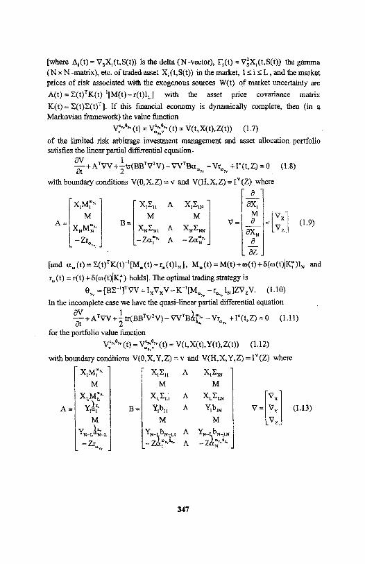
[where is the delta (N-vector), the gamma (N x N -matrix), etc. of traded asset X(t,S(t)) in the market, and the market prices of risk associated with the exogenous sources W(t) of market uncertainty are

with the asset price covariance matrix

If this financial economy is dynamically complete, then (in a Markovian framework) the value function

(1.7)

of the limited risk arbitrage investment management and asset allocation portfolio satisfies the linear partial differential equation

(1.8)

with boundary conditions and where

[and and

holds]. The optimal trading strategy is

(1.10)

In the incomplete case we have the quasi-linear partial differential equation

for the portfolio value function

with boundary conditions where

347

(1.9)

(1.11)

(1.12)

(1.13)

and

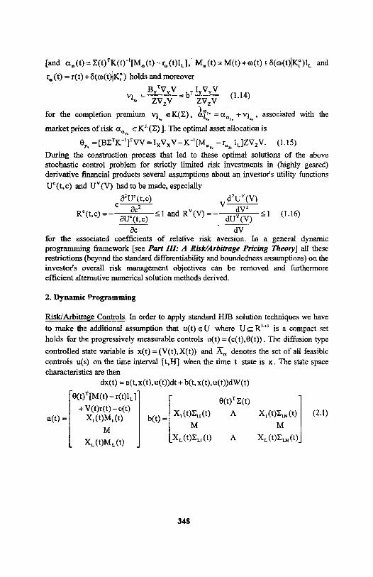
[and and

holds and moreover

for the completion premium associated with the

market prices of risk The optimal asset allocation is

During the construction process that led to these optimal solutions of the above stochastic control problem for strictly limited risk investments in (highly geared) derivative financial products several assumptions about an investor’s utility functions

Uc(t,c) and U’(V) had to be made, especially

for the associated coefficients of relative risk aversion. In a general dynamic programming framework [see Part III: A Risk/Arbitrage Pricing Theory] all these restrictions (beyond the standard differentiability and boundedness assumptions) on the investor’s overall risk management objectives can be removed and furthermore efficient alternative numerical solution methods derived.

2. Dynamic Programming

Risk/Arbitrage Controls. In order to apply standard HJB solution techniques we have to make the additional assumption that where is a compact set holds for the progressively measurable controls The diffusion type

controlled state variable is and denotes the set of all feasible controls u(s) on the time interval [t,H] when the time t state is x. The State space characteristics are then

348

(1.15)

(1.16)and

92.1)

(1.14)

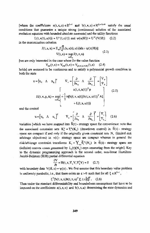
[where the coefficients satisfy the usual conditions that guarantee a unique strong (continuous) solution of the associated evolution equation with bounded absolute moments] and the utility functions

(2.2) in the maximization criterion

[we are only interested in the case where for the value function

(2.4) holds] are assumed to be continuous and to satisfy a polynomial growth condition in both the state

and the control

variables [which we have mapped into - strategy space for convenience: note that

the associated constraint sets (drawdown control) in - strategy space are compact if and only if the originally given constraint sets N, (limited risk arbitrage objectives) in v(t)- strategy space are compact whereas in general the

risk/arbitrage constraint transforms in ë(t) - strategy space are

(infinite) convex cones generated by Ix(t)(Nt)-rays emanating from the origin]. Key to the dynamic programming approach is the second order, non-linear Hamilton-Jacobi-Bellman (HJB) partial differential equation

(2.7)

with boundary data We first assume that this boundary value

is uniformly parabolic, i.e., that there exists an ? > 0 such that for all

(2.8)

Then under the standard differentiability and boundedness assumptions that have to be imposed on the coefficients a( t, x, u) and b( t, x, u) determining the state dynamics and

349

(2.3)

and

92.5)

(2.6)

. problem

and

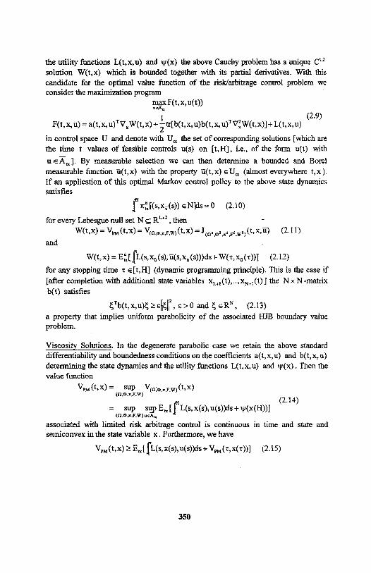
the utility functions L(t,x,u) and ?(x) the above Cauchy problem has a unique C1,2 solution W(t,x) which is bounded together with its partial derivatives. With this candidate for the optimal value function of the risk/arbitrage control problem we consider the maximization program

(2.9)

in control space U and denote with U? the set of corresponding solutions [which are the time t values of feasible controls u(s) on [t,H], i.e., of the form u(t) with

By measurable selection we can then determine a bounded and Borelmeasurable function ?(t,x) with the property (almost everywhere t,x ). If an application of this optimal Markov control policy to the above state dynamics satisfies

(2.10)

for every Lebesgue null set , then

(2.11) and

for any stopping time (dynamic programming principle). This is the case if [after completion with additional state variables matrix b(t) satisfies

(2.13) a property that implies uniform parabolicity of the associated HJB boundary value problem.

Viscosity Solutions. In the degenerate parabolic case we retain the above standard differentiability and boundedness conditions on the coefficients a( t, x, u) and b(t, x, u) determining the state dynamics and the utility functions L(t,x,u) and ?(x). Then the value function

associated with limited risk arbitrage control is continuous in time and state and semiconvex in the state variable x. Furthermore, we have

(2-15)

350

(2.12)

(2.14)

].

] the N X N

and

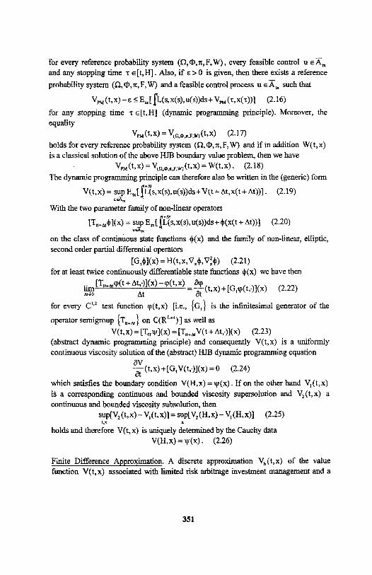
for every reference probability system ( Ω,Φ,π, F,W), every feasible control and any stopping time Also, if ε > 0 is given, then there exists a reference

probability system ( Ω,Φ,π, F, W) and a feasible control process ? such that

(2.16)

for any stopping time (dynamic programming principle). Moreover, the equality

(2.17)

holds for every reference probability system ( Ω,Φ,π, F, W) and if in addition W(t, x) is a classical solution of the above HJB boundary value problem, then we have

(2.18)

The dynamic programming principle can therefore also be written in the (generic) form

(2.19)

With the two parameter family of non-linear operators

(2.20)

on the class of continuous state functions φ (x) and the family of non-linear, elliptic, second order partial differential operators

(2.21) for at least twice continuously differentiable state functions φ (x) we have then

(2.22)

for every C1.2 test function ϕ (t,x) [i.e., Gt is the infinitesimal generator of the

operator semigroup on as well as

(2.23) (abstract dynamic programming principle) and consequently V(t,x) is a uniformly continuous viscosity solution of the (abstract) HJB dynamic programming equation

(2.24)

which satisfies the boundary condition If on the other hand V1(t,x)

is a corresponding continuous and bounded viscosity supersolution and V2(t,x) a continuous and bounded viscosity subsolution, then

(2.25)

holds and therefore V(t, x) is uniquely determined by the Cauchy data

(2.26)

Finite Difference Approximation. A discrete approximation Vh(t,x) of the value function V(t,x) associated with limited risk arbitrage investment management and a

351

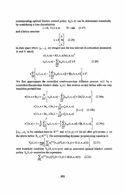
corresponding optimal Markov control policy can be determined numerically by considering a time discretization

(2.27) and a lattice structure

(2.28)

in state space where j0,..,jL are integers and the two relevant discretization parameters

h and δ satisfy

(2.29)

We first approximate the controlled continuous-time diffusion process x(t) by a

controlled discrete-time Markov chain xh(t) that evolves on this lattice with one step transition probabilities

(2.30a)

(2.30b)

(2.30c)

[e0,..,eL is the standard basis in RL+1 and for all other grid points y on

the above lattice ]. The corresponding dynamic programming equation is

(2.31)

with boundary condition and an associated optimal Markov control

policy maximizes the expression

(2.32)

352

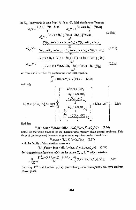
in [backwards in time from H-h to 0]. With the finite differences

(2.33a)

(2.33b)

we then also discretize the continuous-time HJB equation

(2.34)

(2.33c)

and with

find that

(2.35)

(2.36) holds for the value function of the discrete-time Markov chain control problem. This form of the associated dynamic programming equation can be rewritten as

(2.37) with the family of discrete-time operators

(2.38)

for bounded state functions φ (x) on the lattice which satisfies

for every C1,2 test function ϕ (t,x) (consistency) and consequently we have uniform convergence

353

(2.39)

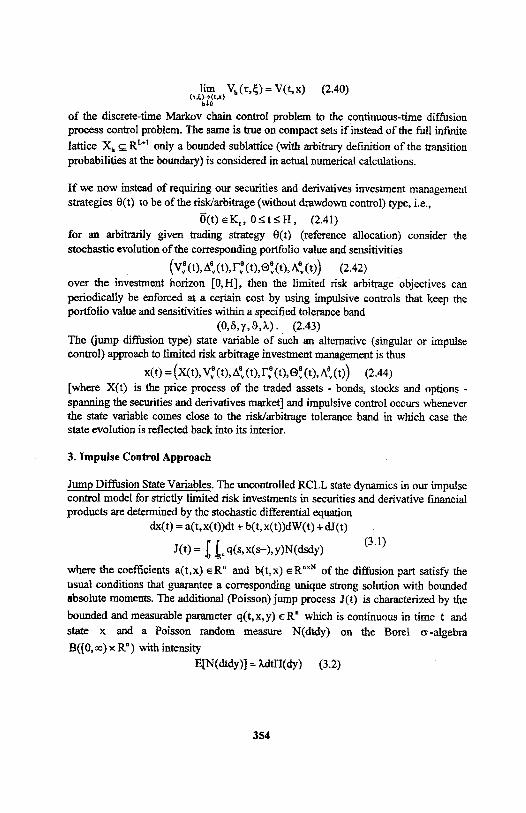
(2.40)

of the discrete-time Markov chain control problem to the continuous-time diffusion process control problem. The same is true on compact sets if instead of the full infinite

lattice only a bounded sublattice (with arbitrary definition of the transition probabilities at the boundary) is considered in actual numerical calculations.

If we now instead of requiring our securities and derivatives investment management strategies θ (t) to be of the risk/arbitrage (without drawdown control) type, i.e.,

(2.41)

for an arbitrarily given trading strategy θ (t) (reference allocation) consider the stochastic evolution of the corresponding portfolio value and sensitivities

(2.42) over the investment horizon [0,H], then the limited risk arbitrage objectives canperiodically be enforced at a certain cost by using impulsive controls that keep theportfolio value and sensitivities within a specified tolerance band

(2.43) The (jump diffusion type) state variable of such an alternative (singular or impulse control) approach to limited risk arbitrage investment management is thus

(2.44) [where X(t) is the price process of the traded assets - bonds, stocks and options - spanning the securities and derivatives market] and impulsive control occurs whenever the state variable comes close to the risk/arbitrage tolerance band in which case the state evolution is reflected back into its interior.

3. Impulse Control Approach

Jump Diffusion State Variables. The uncontrolled RCLL state dynamics in our impulse control model for strictly limited risk investments in securities and derivative financial products are determined by the stochastic differential equation

(3.1)

where the coefficients a and of the diffusion part satisfy the usual conditions that guarantee a corresponding unique strong solution with bounded absolute moments. The additional (Poisson) jump process J(t) is characterized by the

bounded and measurable parameter which is continuous in time t and

state x and a Poisson random measure N(dtdy) on the Borel σ -algebra

with intensity

(3.2)

354

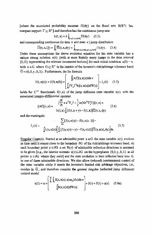
[where the associated probability measure

compact support ] and therefore has the continuous jump rate

(3.3)

and corresponding continuous (in time t and state x) jump distribution

(3.4)

Under these assumptions the above evolution equation for the state variable has a unique strong solution x(t) [with at most finitely many jumps in the time interval [0, H] representing the relevant investment horizon] for each initial condition x(0) = x

with x ε G where G ⊆ Rn is the interior of the investor’s risk/arbitrage tolerance band

Furthermore, the Ito formula

(3.5)

holds for C1,2 functionals f(t,x) of the jump diffusion state variable x(t) with the associated integro-differential operator

(3.6)

and the martingale

(3.7)

Singular Controls. Started at an admissible point the state variable x(t) evolves

in time until it comes close to the boundary ? G of the risk/arbitrage tolerance band. At each boundary point a set R(y) of admissible reflection directions is assumed

to be given [e.g., the interior normals on the hyperplanes (0 ,δ,γ,ϑ,λ) at all

points where they exist] and the state evolution is then reflected back into G

in one of these admissible directions. We also allow (relaxed) inter-temporal control of the state variable while it meets the investor’s limited risk arbitrage objectives, i.e.,

resides in ?, and therefore consider the general singular (reflected jump diffusion) control model

(3.8a)

355

on the Borel sets B(Rn) has

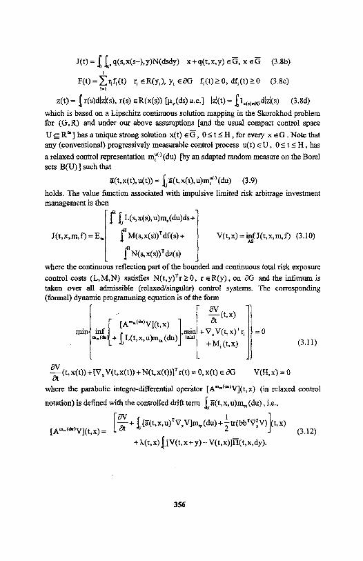
(3.8b)

(3.8c)

(3.8d) which is based on a Lipschitz continuous solution mapping in the Skorokhod problem for (G,R) and under our above assumptions [and the usual compact control space

] has a unique strong solution for every . Note that any (conventional) progressively measurable control process , has

a relaxed control representation [by an adapted random measure on the Borel

sets B(U)] such that

(3.9)

holds. The value function associated with impulsive limited risk arbitrage investment management is then

(3.10)

where the continuous reflection part of the bounded and continuous total risk exposure

control costs (L,M,N) satisfies on ?G and the infimum is taken over all admissible (relaxed/singular) control systems. The corresponding (formal) dynamic programming equation is of the form

where the parabolic integro-differential operator [Amtx(du)V](t,x) (in relaxed control

notation) is defined with the controlled drift term , i.e.,

(3.12)

356

(3.11)

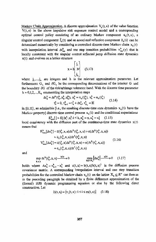
Markov Chain Approximation . A discrete approximation Vh (t, x) of the value function V(t,x) in the above impulsive risk exposure control model and a corresponding

optimal control policy consisting of an ordinary Markov component a

singular control component and an associated reflection component can be

determined numerically by considering a controlled discrete-time Markov chain xh (t)

with interpolation interval and one step transition probabilities that is

locally consistent with the singular control reflected jump diffusion state dynamics x(t) and evolves on a lattice structure

(3.13)

where j1,..,jn are integers and h is the relevant approximation parameter. Let

furthermore Gh and ∂ Gh be the corresponding discretizations of the interior G and

the boundary ∂ G of the risk/arbitrage tolerance band. With the discrete time parameter k = 0,1,2,..,Kh enumerating the interpolation steps

(3.14)

in [0, H], an admissible [i.e., the resulting discrete-time state dynamics xh(t) have the

Markov property] discrete-time control process uh (t) and the conditional expectations

(3.15) local consistency with the diffusion part of the continuous-time state dynamics x(t) means that

and

(3.17)

holds where and is the diffusion process covariance matrix. A corresponding interpolation interval and one step transition

probabilities for the controlled Markov chain xh(t) on the lattice can then as in the preceding paragraph be obtained by a finite difference approximation of the (formal) HJB dynamic programming equation or else by the following direct construction. Let

(3.18)

357

(3.16)

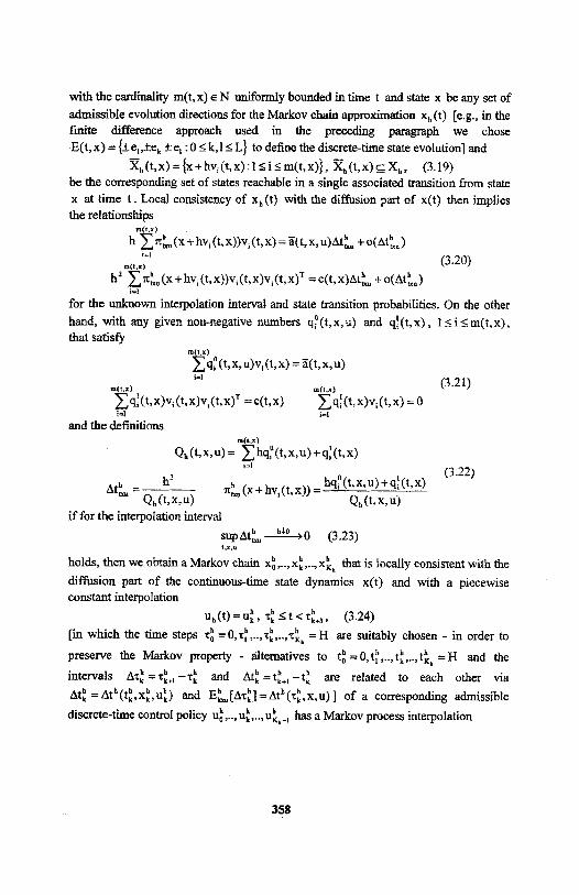
with the cardinality m(t, x) ε N uniformly bounded in time t and state x be any set of

admissible evolution directions for the Markov chain approximation xh(t) [e.g., in the finite difference approach used in the preceding paragraph we chose

to define the discrete-time state evolution] and

(3.19) be the corresponding set of states reachable in a single associated transition from state

x at time t . Local consistency of xh(t) with the diffusion part of x(t) then implies the relationships

(3.20)

for the unknown interpolation interval and state transition probabilities. On the other

hand, with any given non-negative numbers and that satisfy

(3.21)

and the definitions

(3.22)

if for the interpolation interval

(3.23)

holds, then we obtain a Markov chain that is locally consistent with the

diffusion part of the continuous-time state dynamics x(t) and with a piecewise constant interpolation

(3.24)

[in which the time steps are suitably chosen - in order to

preserve the Markov property - alternatives to and the

intervals and are related to each other via

and of a corresponding admissible

discrete-time control policy has a Markov process interpolation

358

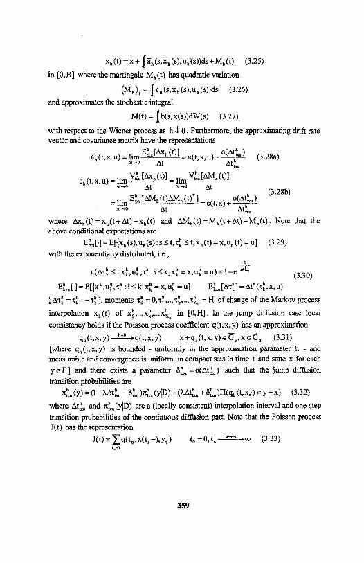
(3.25)

in [0, H] where the martingale Mh(t) has quadratic variation

(3.26)

and approximates the stochastic integral

(3.27).

with respect to the Wiener process as h ↓ 0. Furthermore, the approximating drift rate vector and covariance matrix have the representations

(3.28b)

Note that the above conditional expectations are

(3.29)

with the exponentially distributed, i.e.,

(3.30)

moments of change of the Markov process

interpolation xh(t) of in [0, H] . In the jump diffusion case local

consistency holds if the Poisson process coefficient q(t,x, y) has an approximation

(3.31)

[where qh(t,x,y) is bounded - uniformly in the approximation parameter h - and

measurable and convergence is uniform on compact sets in time t and state x for each

] and there exists a parameter such that the jump diffusion

transition probabilities are

(3.32)

where and are a (locally consistent) interpolation interval and one step

transition probabilities of the continuous diffusion part. Note that the Poisson process J(t) has the representation

(3.33)

359

93.28a)

where and

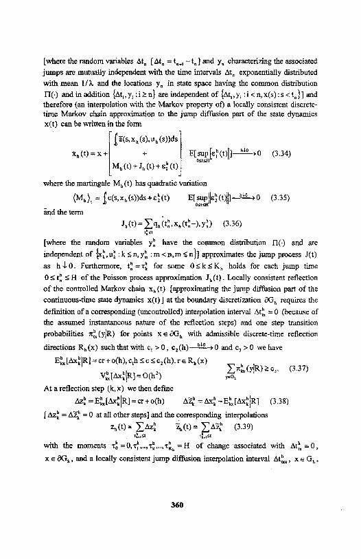
[where the random variables and yn characterizing the associated

jumps are mutually independent with the time intervals exponentially distributed

with mean l/ λ, and the locations yn in state space having the common distribution

Π(⋅) and in addition are independent of and therefore (an interpolation with the Markov property of) a locally consistent discrete- time Markov chain approximation to the jump diffusion part of the state dynamics x(t) can be written in the form

(3.34)

where the martingale Mh(t) has quadratic variation

and the term

(3.36)

[where the random variables yhn have the common distribution Π(−) and are

independent of approximates the jump process J(t)

as h ↓ 0. Furthermore, for some holds for each jump time

of the Poisson process approximation Jh(t). Locally consistent reflection

of the controlled Markov chain xh(t) [approximating the jump diffusion part of the

continuous-time state dynamics x(t)] at the boundary discretization δ Gh requires the

definition of a corresponding (uncontrolled) interpolation interval (because of

the assumed instantaneous nature of the reflection steps) and one step transition

probabilities for points x ∈ ∂ Gh with admissible discrete-time reflection

directions Rh(x) such that with we have

(3.37)

At a reflection step (k, x) we then define

(3.38)

at all other steps] and the corresponding interpolations

(3.39)

with the moments of change associated with

, and a locally consistent jump diffusion interpolation interval

360

(3.35)

and

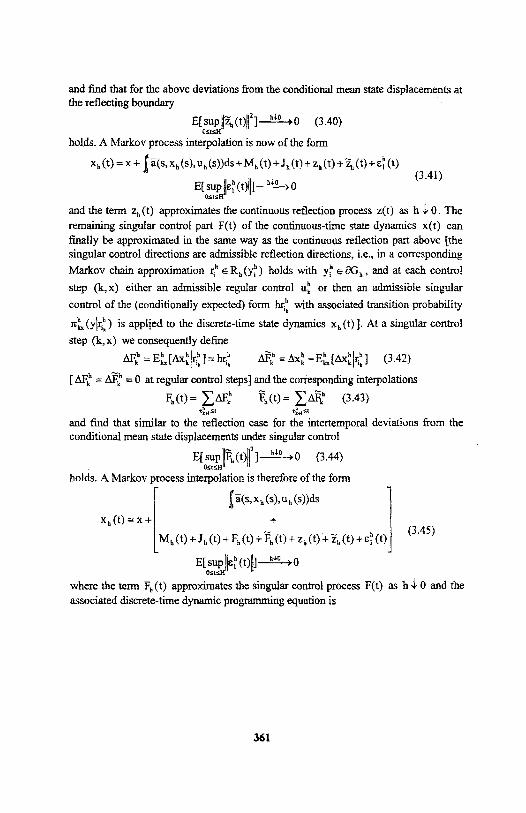
and find that for the above deviations from the conditional mean state displacements at the reflecting boundary

(3.40)

holds. A Markov process interpolation is now of the form

(3.41)

and the term zh(t) approximates the continuous reflection process z(t) as h ↓ 0. The

remaining singular control part F(t) of the continuous-time state dynamics x(t) can finally be approximated in the same way as the continuous reflection part above [the singular control directions are admissible reflection directions, i.e., in a corresponding

Markov chain approximation holds with , and at each control

step (k,x) either an admissible regular control uhk or then an admissible singular

control of the (conditionally expected) form hr h ik with associated transition probability

is applied to the discrete-time state dynamics xh(t)]. At a singular control

step (k, x) we consequently define

(3.42)

at regular control steps] and the corresponding interpolations

(3.43)

and find that similar to the reflection case for the intertemporal deviations from the conditional mean state displacements under singular control

(3.44)

holds. A Markov process interpolation is therefore of the form

(3.45)

where the term Fh(t) approximates the singular control process F(t) as h ↓ 0 and the associated discrete-time dynamic programming equation is

361

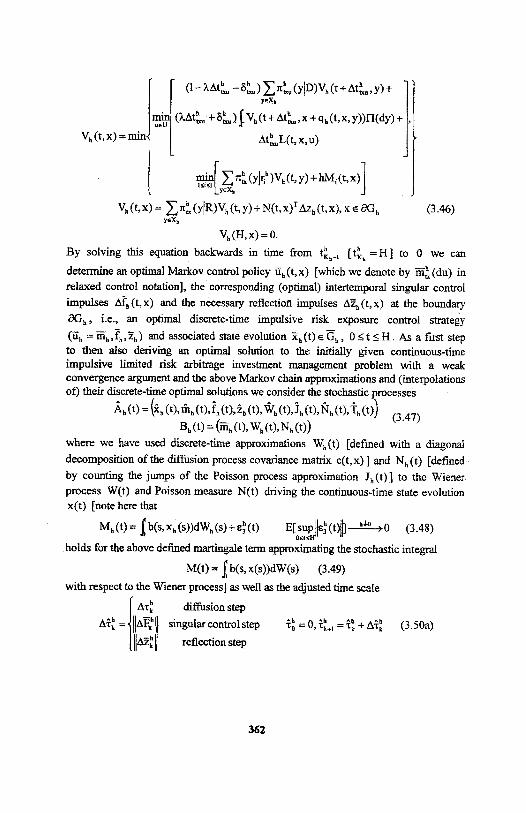
(3.46)

By solving this equation backwards in time from to 0 we can

determine an optimal Markov control policy [which we denote by in

relaxed control notation], the corresponding (optimal) intertemporal singular control

impulses and the necessary reflection impulses at the boundary

∂ Gh, i.e., an optimal discrete-time impulsive risk exposure control strategy

and associated state evolution As a first step to then also deriving an optimal solution to the initially given continuous-time impulsive limited risk arbitrage investment management problem with a weak convergence argument and the above Markov chain approximations and (interpolations of) their discrete-time optimal solutions we consider the stochastic processes

(3.47)

where we have used discrete-time approximations Wh(t) [defined with a diagonal

decomposition of the diffusion process covariance matrix c(t,x)] and Nh(t) [defined

by counting the jumps of the Poisson process approximation Jh(t)] to the Wiener

process W(t) and Poisson measure N(t) driving the continuous-time state evolution x(t) [note here that

(3.48)

holds for the above defined martingale term approximating the stochastic integral

(3.49)

with respect to the Wiener process] as well as the adjusted time scale

diffusion step

singular control step (3.50a)

reflection step

362

for diffusion steps

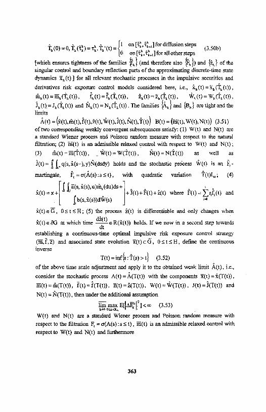
for all other steps (3.50b)

[which ensures tightness of the families (and therefore also and of the singular control and boundary reflection parts of the approximating discrete-time state

dynamics for all relevant stochastic processes in the impulsive securities and

derivatives risk exposure control models considered here, i.e.,

and The families and are tight and the limits

(3.51)

of two corresponding weakly convergent subsequences satisfy: (1) W(t) and N(t) are

a standard Wiener process and Poisson random measure with respect to the natural filtration; (2) is an admissible relaxed control with respect to W(t) and N(t) ;

(3) as well as

holds and the stochastic process is an

martingale, with quadratic variation (4)

where and

(5) the process is differentiable and only changes when

at which time holds. If we now in a second step towards

establishing a continuous-time optimal impulsive risk exposure control strategy

and associated state evolution , define the continuous inverse

(3.52)

of the above time scale adjustment and apply it to the obtained weak limit i.e.,

consider the stochastic process with the components

and

, then under the additional assumption

W(t) and N(t) are a standard Wiener process and Poisson random measure with

respect to the filtration is an admissible relaxed control with

respect to W(t) and N(t) and furthermore

363

(3.53)

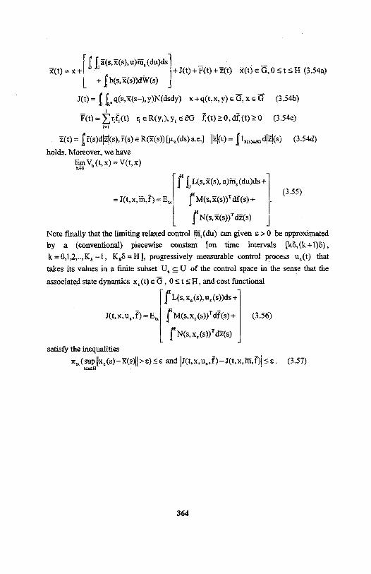
(3.54a)

(3.54b)

(3.54c)

(3.54d)

holds. Moreover, we have

(3.55)

Note finally that the Limiting relaxed control can given ε > 0 be approximated

by a (conventional) piecewise constant [on time intervals

, progressively measurable control process u ε (t) that

takes its values in a finite subset U2 ⊆ U of the control space in the sense that the

associated state dynamics , and cost functional

(3.56)

satisfy the inequalities

(3.57)

364

and

Appendix: References

[1] M. H. A. Davis, Martingale Methods in Stochastic Control, Lecture Notes in Control and Information Sciences 16, Springer 1978

[2] P. L. Lions and A. S. Sznitman, Stochastic Differential Equations with Reflecting Boundary Conditions, Communications on Pure and Applied Mathematics 37, 511-537 (1984)

[3] J. P. Lehoczky and S. E. Shreve, Absolutely Continuous and Singular Stochastic Control, Stochastics 17, 91-109 (1986)

[4] H. J. Kushner, Numerical Methods for Stochastic Control Problems in Continuous Time, SIAM Journal of Control and Optimization 28, 999-1048 (1990)

[5] B. G. Fitzpatrick and W. H. Fleming, Numerical Methods for an Optimal Investment-Consumption Model, Mathematics of Operations Research 16, 823-841 (1991)

[6] N. El Karoui and I. Karatzas, A New Approach to the Skorohod Problem, and its Applications, Stochastics and Stochastics Reports 34, 57-82 (1991)

[7] P. Dupuis and H. Ishii, On Lipschitz Continuity of the Solution Mapping to the Skorokhod Problem, with Applications, Stochastics and Stochastics Reports 35, 31-62 (1991)

[8] M. G. Crandall, H. Ishii and P.-L. Lions, User’s Guide to Viscosity Solutions of Second Order Partial Differential Equations, Bulletin of the American Mathematical Society 27, 1-67 (1992)

[9] J. Ma, Discontinuous Reflection, and a Class of Singular Stochastic Control Problems for Diffusions, Stochastics and Stochastics Reports 44, 225-252 (1993) [10] J. Ma, Singular Stochastic Control for Diffusions and SDE with Discontinuous Paths and Reflecting Boundary Conditions, Stochastics and Stochastics Reports 46, 161-192 (1994) [11] W. H. Fleming and H. M. Soner, Controlled Markov Processes and Viscosity Solutions, Applications of Mathematics, Springer 1993 [12] H. J. Kushner and P. G. Dupuis, Numerical Methods for Stochastic Control Problems in Continuous Time, Applications of Mathematics, Springer 1992 [13] R. J. Elliott, Stochastic Calculus and Applications, Applications of Mathematics, Springer 1982 [14] S. N. Ethier and T. G. Kurtz, Markov Processes: Characterization and Convergence, Wiley 1986 [15] J. Jacod and A. N. Shiryayev, Limit Theorems for Stochastic Processes, Grundlehren der mathematischen Wissenschaften, Springer 1987

365