Embed Size (px)
Citation preview

Journal of Financial Economics 21(1988) 255-289. North-Holland
RISKANDRE~wiAN Application d a New Test M&hoddogy*
Gregory CONNOR hivemity ojCahifbmia, Berkeley, CA 94720, USA
Robert A. ICOlUUCZYK Northwestem hive&@, Evamton, IL 602@ USA
Received June 1986, final version received March 1988
We *use an asymn*fiG c_& p?&@$ ~~~nentc terhniqrw tc Pctimate t-&p xy~~oiv~ &pm= inffwc- r--‘-- __--I.__ _____ mg asset returns and to test the restrictions imposed by static and intertemporal e@ib&un versions of the arbitrage pricing theory (APT) on a multivariate regre&on tnodel, me cm@&$!! techniques allow for fairly arbitrary time variation in risk premiums. We Gnd that the AR?_ provides a -better description of the expected returns on assets & thg ca$%L asset oricing mode! (CAPM). However, some statistically reliable m&pricing of assets by the APT rem&s.
In this paper we estimate and test the restrictions implied by an equilibrium version of Ross’s arbitrage pricing theory (APT). We estimate the return factors using the asymptotic principal components technique first suggested by Chamberlain ar& Rothschild (1983) and extended by Concur and Korajczyk (1986). We test tie cross-sectional restrictions imposed by the APT with a variety of multivariate procedures.
Section 2 describes the APT specification that we test. We use both the standard, s&atic version of the APT and an intertemporal version developed in Connor and Korajczyk (1987). In this second version there is one factor that has a unit beta for every security. The static version does not impose this unit-beta restriction.
*We would like to thank Sankarshan Acharya, Gary Chamberlain, Lawrexe Harris, Robert Zxhick, Ravi Jagannathan, Donaid Keim, Ahan J&idon, Bruce Lchn~annt Craig Ma&inlay, Robert McDonald, Jay Shanken, Daniel Siegel, an anonymous referee, and the editor, John Long, for generous comments and suggestions The paper also benefited from discussions with the seminar participants at University of Alberta, Carnegie-Mellon University, University of Chicago, INSEAD, University of Minnesota, Northwestern University, University of Pennsylvania, South- em Methodist University, Stauf’ord University, and University of Southern California. l’he usuai caveat applies.
0304405X/88/$3.50@ 1988, EGevier Science Publishers B.V. (North-Hol!and)
256 G. Connor and RA. Korajczyk, Rhk and return in an equilibrium APT
In section 3 we outline the asymptotic principal components technique that we use to estimate the pervasive economic factors and a new iterative version that is more efficient than the one-step procedure described in Connor and Korajczyk (1986). These factor estimates are valid in a model with time-vary- ing risk premiums, as long as asset betas are constant. ‘Vte estimate the return factors and relate them to mrne macroeconomic time series suggested as possible sources of pervasive economic risk by Chen, Roll, and Ross (1986). We also analyze the estimation error in the factors using our technique and discuss the relationship between our method and standard factor analysis.
Iri section 4 we describe our testing procedures and empirical results. We use large cross-sectional samples (between 1,487 and 1,745 f?ums), both grouped into size-based potiolios and at the individual seclurity level, to test the model. We **rform tests using the &aggregated data by placing prior restrictions on the covariance matrix of residuals. The techniques are also applied to the CAPM, using standard proxies for the market portfolio. The APT explains the anomalous size-related season&l patterns in returns that have been docu- mented by others, although some nonseasonal anomalies persist. We conclude with a summary and suggestions for extensions.
We briefly describe the asset pricing model to be tested. More detailed discussion of the APT can be found in Ross (1976), Chamberlain and Rothschild (1983), and Connor (1984). Let c denote the muntably infinite vector of returns to a countably infinite set of traded assets. Assume that asset retqums follow an approximate factor model,
(1) E( stlft ) = 0, E( 6) = 0; E( $g;) = V,
where ty is a k-vector of pervasive economic factors, B is an 00 X k matrix of the factor sensitivities of the assets, and St is the vector of idiosyncratic returns.
Let B” denote the first n rows of B and V” denote the first n rows and columns of K Let 11 l 11 denote the matrix L*-norm? Assume that
’ 1 I( ) -1
-pp
n <Cl< co foralln,
for all 3,
G. Connor atad R.A. Kwajczyk, Risk and return in an equilibrium APT 257
and that there is a cross-sectional average idiosyncratic variance
where plim denotes the Iimit in probability. The equilibrium version* of the AFT implies that
1) 2
where rFt represents the return on a riskless asset, e is a vector of ones, and yt is a k-+~~~tor of factor risk premiums.
Combining equations (1) and (2) gives
L
rr - rFte = B( yt +l) + &=
The relation (3j provides us with the basis for testing the restrictions imphed by the modeI.
Let B” denote an n X 2’ matrix ccmisthg of the observed returris on r’i assets over T’ periods. Let rF denote a T-vector of observed returns on the riskless asset. The n X T matrix of excess returns (returns in excess of the riskless return) is given by R* = r* - e?$. Using (3j we can write the excess returns as
R”=B”F+P, (4)
where F is the k x T matrix of realizations of (u, +ft) over the period and E” is the n X T .mati of realizations of et. In the empirical specification of the APT used here we aflow for time variation in factor risk premiums (u,) but assume that factor sensitivities (B*) are time-invariant.
In Connor and Korajczyk (1986) we describe a new technique for identify- ing st~tisticaUy the pervasive LLUG, plus their associated risk premiums, assumed by the APT. We cwi -11 th& approach asymptotic principal contponent~. It is similar to standard principal components except that it reiies on asymp- totic results as the number of cross-sections grows large. In this section, we briefly review the relevant results from that paper9 develop a more efficient - -
2The distinction between the sta~dsrd AF’I’ Ed equilibrium versions of the APT is that the stmdtid tiikage conditions imply that (2) holds as an approximation whereas the equilibrium models [e.g., Connor (1984)J use additional restrictior45 0~ t23tes md supplies of assets to derive (2) as an equdity. St! Sha&m (i985bj for a discussion of this distinction. I
258 G. Connor and R.A. Korajczyk, Risk and return in an equilibrium APT
version of the estimator, and show that the technique is valid for models with time-varying risk pretiums. In addition we compare our estimated Factors with some standard market indices and a set of macroeconomic time series suggested M sources of pervasive economic risk by Chen, Roll, and Ross (1986).
3.1. Asymptotic principal components
Denote the TX T cross-product matrix &!” = (l/n)RVE We apply a result from Connor and Korajczyk (1986) about the eigenvectors of 0”. Let G” denote the orthonormal k X I!' matrix consisting of the first k eigenvectors of Qn. We show that G” is approximately a nonsirgu!-r linear transformation of F.
Theorem 1. Gn = LnF+ $n, where L” is a nonsingular matrix for dt n and Plim ,, -, &” = 0, the zero matrix.
Theorem 1 is based on the result from Chamberlain and Rothschild (1983) that, as the number of cross-sections grows large, eigenvector analysis is asymptotically equivalent to factor analysis. Note that we can determine F only up to a nonsingular linear transformation, Ln - this reflects the ‘rota- tional indeterminacy’ of factor mo&%_
A simple example may be useful in providing some intuition for this result. The simplest case with which we can deal has one pervasive factor and two time periods, i.e.,
wi,=bi(Yg+_f) .I &irt i=1,2,3 ,..., t=1,2.
Note that the risk premiums, yr, can vary through time arbitrarily, but are not separately identifiable from the mean-zero factor realization, f;. In the exam- ple $2” is a 2 x 2 matrix whose (t, I) element is equal to
The diagonal elements are given ‘_‘y
f +2,-,: -PL) ( ’ fj biEi7/n 7 = 1,2. i=l I’
. 0

G. Connor and R.A. Korajczyk, Risk and return in an equi&!wn APT 259
The oif-diagonal tzrms in &P are given by
Under our assumptions, the (cross-sectional) average squared beta converges (as n + 00) to some value, say 6’, and the (cross-sectional) average &;I converges to Q ? By the assumption of an approximate factor structure and temporally independent E’S, the last term in (5) and the last three terms iz~ (6) mnverge (again as n + 00) to zero. Therefore, as n - 00, &P converges to
$J=p r (Yl+A)2 I
(n +m2 +A)
(Yl +f;)(uz +a (y2+Q2 +a21,. I
(7)
The limit matrix, Q, contains all of the information we seek, [i.e., (yq +A) and (y2 +&)I. We merely need a means of extracting t&is information. tie reader can check that the first eigenvector of Q is proportional to the vector of realized factors plus their risk premiums.
3.2. New extensions of the technique
Here we offer a refinement, in terms of estimation efficiency, to our asymptotic principal components technique and show that the factor estimates allow for time-varying risk premiums.
We motivate our refinement by considering a well-known relationship between factor anaiysis and standard principal components analysis. Let C denote the true (not estimated) 6 &v&mm matrix of returns and assume that they obey a strict factor mocfel:
=BB’+ V, (8)
where V is assumed to be a diagonal matrix. This is the model used in factor analysis. Pre- and post-multipQ both sides of (8) by V-II2 to get
21” = B”B” + I 9 (9)
of its idiosyncratk returq
as follows. First estimate the factors by
constant). Cal&ate QR8 = (1/n)l’P*‘l’P* and xeestbate G”*. Empirically, our large that CT does not provide much improve- with UMU~~ -sectionaI samples may find
improvement. No@ also, that we must use estimates of the our proof assumes knowledge of the true i
we are allowing n to appro+i inbity, with T fixed, we cannot rely on the standard T-consistency of I? This estimation risk may reduce the eliiciency gain of the procedure.
Recent empirical work suggests that asset risk premiums vary through time [see, e.g., Brown, Kleidon, and Marsh (1983), Keim (1983), Keim and Stambaugh (1986), and Ferson, Kandel, and Stambaugh (1987)]. The a&y&s in section 3.1 assumes that asset returns follow an exact multi-factor asset
‘The pro& is amikhe from the authors. Iu it we use a slightly stronger assumption about t&e ruean square idiosyncratic returns. Let zj = $ - Kj, zE = (q, . . . , z,,)‘, and Q” = ~z”z”‘]. In pbce of plum Pe”/n = u2 we assume hat IIQ”II is bounded for all n.
Weesthatethefactorsandrisk fuur nonoverlapp* h-year ) 1969~1973* 1974-l and 19794983. The choice of toearlierworksuchsBhck, S&&s (1972) iwd Weestimatethef~byapplyia%~toticprincipalcomponentstothe entire sample of New York Stack w (NOSE) and Aukcan Stock BdU@e (AMEX) firms with no missing obsmations over the h-year suWd The numbers of fknx reqkctively, and the number of
1,487,1,720, 1,734, and 1,745, is 60 for each subpakxL4
IiskksreturnisassumedtQbe xeta~~~ on Trwsuy bills from Ibb~tson Associates (1985).
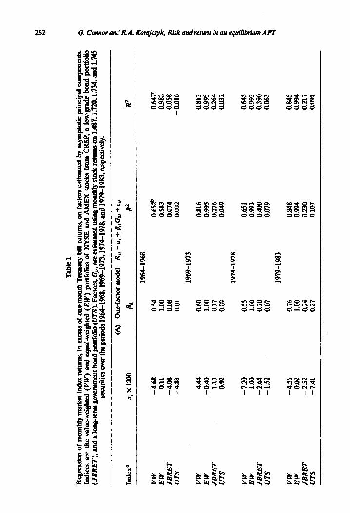
an~~~oftlaebehaviorofthefactorsinreIatitionto standard market portfolio6 we regress the exazss return on the equal-weighted and val~+we$,ked CRSI’ (Center for l&sear& in Security Price@ purtfoIios on the Faust factor, the first five factors, and the Gust ten factors. To faditate comparisons across indices we &&!e ek factors s0 that the equal-weighted CRSP pmtfdio has beitas equd to LO. The estimated intercept term and the R* vahes are invariant to this type of resealing The results for the one-factor ad five-factor regressions are shown in table 1. An interesting feature of these regressions is that the first factor generay explains over 998 of the variancce
‘The reQuirement ihat firms Save no missing observations &mhates about 30% of f&e total CRSP universe of WSE 2rii3 AMEX fums. The aveiage number of firms with returns obsemd in a given month is 2,151,2,474,2,567, and 2,341 in the four subperiods, respectively.
Tab
le 1
Reg
ress
ion
of m
onth
ly m
ark
et iu
dex
retu
rns,
i.. e
xces
s of
one-
mon
th T
reas
ury
bill
ret
urns
, on
fact
ors e
stim
ated
by
asym
ptot
ic p
rinc
ipal
com
poue
nts.
In
dice
s ar
e th
e va
lue-
wei
ghte
d (V
W)
and
equa
Lw
eigh
ted
(EW
) po
rtfo
lios
of N
YS
E a
nd A
ME
X s
tock
s fr
om C
RS
P, a
low
-gra
de b
ond
port
folio
9
(JB
RE
T),
an
d a
long
-ter
m g
over
umen
t bon
d po
rtfo
lio (U
TS)
. F
acto
rs, G
il, a
re e
stim
ated
usi
ng m
onth
ly s
tock
retu
rns OIB 1,
487,
1,72
0,1,
734,
an
d 1,
745
. 0 8
_ _
secu
riti
es ov
er th
e pe
riod
s NM
-1%
8,1%
9Li9
73,1
974-
1978
, ti
d 19
79-1
983,
res
pect
ivel
y.
t
Ind
exa
VW
E
W
JBR
ET
U
TS
VW
E
W
JBR
ET
&
US
VW
E
W
JBR
ET
U
TS
VW
E
W
JBR
ET
U
TS
ai
X 1
200
- 4.
68
0.11
-
4.08
-
4.83
4.44
-0
.40
1.13
0.
92
- 7.
20
1.00
-
2.64
-1
.52
- 4.
56
0.02
-
2.52
-
7.41
(A)
Oue
~fa
ctor
mod
el
Ri,
= a
i +
&C
l, +
&if
Bil
R
2 R
2 -
1964
-196
8
0.54
0.
6szb
O
.&V
1.
00
0.98
3 0.
982
0.08
0.
074
0.05
8 0.
01
0.00
2 -
0.01
6
1969
-197
3
0.60
0.
816
0.81
3 1.
00
0.99
5 0.
995
0.17
0.
276
0.26
4 0.
09
0.04
9 0.
032
1974
-197
8
0.5s
0.
651
0.64
5 1.
00
0.99
3 n
993
-0.-
e_
0.20
0.
400
0.39
0 0.
07
0.07
9 0.
063
1979
-198
3
0.76
0.
848
0.84
5 L
OO
0.
994
0.99
4 0.
24
0.23
0 0.
217
0.27
0,
107
0.09
1
Tab
le 1
(conti
nued
)
i%4-
1%8
3.6
5
1.0
0
- 0.3
4
- 0.6
3
1969-1
973
- 9.6
0
1.0
0
- 19.4
4
13.0
7
1974-1
978
- 3.5
6
1.0
0
-o.g
s l
- 2.0
3
1979-1
983
7.5
4
1.0
0
6.0
1
12.5
9
2.7
7
2.7
1
0.8
97b
1.0
0
1.0
0
0.9
94
1.8
2
- 2.9
5
0.3
54
1.8
2
- 0.5
5
0.1
81
0.8
87c
0.9
93
0.2
95
0.1
06
VW
-
2.6
4
EW
0.7
9
JBR
ET
-
2.2
8
UT
S -3
.24
0.5
3
1.0
0
0.0
7
0.0
0
1.4
9
1.0
0
- 0.1
5
- 1.3
0
VW
0.
85
EW
-
1.20
JB
RE
T
0.67
U
TS
4.49
0.59
5.1
4
l&Q
1.0
0
0.1
7
0.8
3
0.1
0
1.0
1
7.1
3
- 3.
55
1.0
0
1.0
0
- 11.2
6
- 2.
03
- 30.3
7
- 2.
22
0.94
3 0.
938
0.99
7 0.
997
0.3%
0.
340
0.35
1 0.
291
VW
-
5.52
0.
55
6.06
fi’
h’;
0.56
1.0
0
1.0
0
JBR
ET
-
2.52
0.
20
2.09
U
TS
- 0.
63
0.07
1.
31
- 5.
09
2.83
0.
966
0.96
2 1.0
0
LO
O
0.99
8 0.
998
1.0
9
87.7
3 0.
591
0.55
3 -
1.6
2
- 2.
16
0.26
2 0.1
94
VW
-:
.a2
EW
0.
06
JBR
ET
II
3m
- L
.L6
[.!T
S -
6.85
0.76
-
3.86
1.0
0
i.00
0.24
4.
27
027
8.40
- 0.
03
- 1.5
9
0.94
6 1.0
0
1.0
0
0.99
8 4.
28
2.85
0.
523
6.11
5.
46
0.48
5
0.9
41
0.9
97
0.4
79
0.43
7
‘The
fact
or e
stim
ates
, Gjt
, are
sca
led so
that
the eq
mhvei
ghte
d C
RSP
port
foli
o has
a u
nit
bet
a fo
r ea
ch fa
ctor.
This scaling has no ef
fect
on the
esti
mat
es of
Qi o
r R
*.
bUna
djus
ted
R’.
‘A
Bju
sted
R’.
264 G. Connor and RA. Korajczyk Risk and return in an equilibtium A Pi-
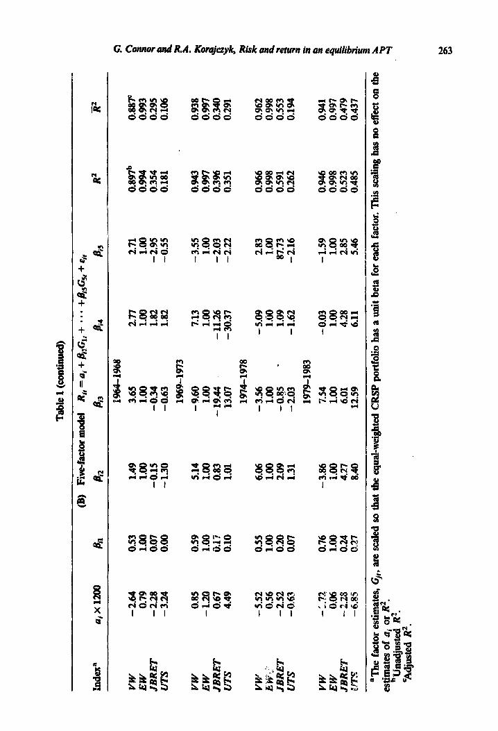
of &C +&w&@d portfolio. The remaining factors have statistically sig- ticant explanatory power (see table 2) but obviously explain much less of the v&au*. l?or the value-weighted portfolio the results are quite Merent. The first factor still explains most of the variance of the portfolio, but much less than it does for the equ&weighted portfolio. The additicna! factors, a@n, are
“iinportmt. Howevr, even with ten factors we do not reach an R* value obtained in the relation of the =weighted portfolio with just one factor?
Table 1 also inciudes the of regmsiq the excess returns of a portfolio of bo& wjth ratings below Baa (denoted JBRET) and the excess returns on long-term government bonds (denoted UTS) on the factor esti- mates. These data are from Ibbotson (1979) and Ibbotson Associates (1985), res~pectively..Simila~ variabks were founk zc be important factors (in explain- ing cross-se~tioual di&renm in mean returns) by Chen, Roll, and Ross (1986). For JBRET we use returns in excess of the riskless rate, whereas their variable UPR uses returns in excess of the return on an Aaa bond portfolio. The first factor exphGns between 7% and 40% of the variance of the junk bond returns and the first five factors explain Wtween 35% and 59% of the variaue. The sixth through tenth factors do not have significant explanatory power.
The factors explain less of the variability in the excess returns on long-term government bonds than they do for the other indexes. The first factor exulains between 0% and 11% of UTS and the first five factors explain between 18% aud 49% of the variation. The sixth through tenth factors do not have sign&ant explanatoq power except in the 1974-1978 subperiod.
The high correlation between our factor estimates and the stock and bond market indices is not sufficient to guarantee that- we will pick up the same cross-sectional pricing relation as Chen, Roll, and Ross (1986). However, I& of correlation might indicate that our factor estimates omit important priced factors. Thus, we view the correlations in table 1 as encouraging in the sense
. that a necessary (but not s&Went) condition for *consistency with Chen, Roll, and Ross is met.
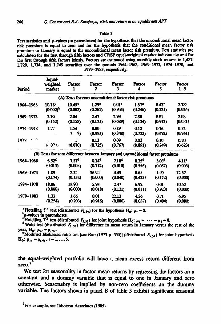
Some previous empirical studies have drawn inferences about the validity of ahe APT by testig w&her *he estimated factor risk premiums are different from zero, on average. Although this is not the approach we take, individual and joint tests of whether the unconditional means of the factors are equal to zero are presented in panel A of table 3 for the sake of comparison with earlier work. Equivalent tests are also shown for the equal-weighted stock portfolio. The test that the means of the first five factors arc jointly zero (last column) is @@cant at the 10% level in the first two subperiods and not signScant in the last two. egating across the four subperiods yields a statistic that is significant at the 10% level. In general, the results in panel A of table 3 seem to
‘We estimate these same regressions using factors esti.mated by the iterative procedure de- scribed above. Note that in calculating sz”* each scurity if w&&ted inv~r+ -*---%=ml l e i+* Gil )Pnuil’-V-~ rr- &V S&G idiosyncratic variance. This will tend to place less weight on small firms in relation to large firms. Since the results are ~.%tudly identical to the results in table 1, we do not report them kre.
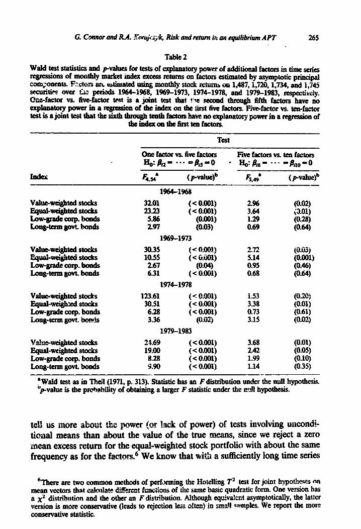
Table 2
Wald test statistics and p-valws for tests of explanatory power of additional factors in time series qressions of mo&ly market hdcx excess retums on factors estimated by asymptotic principal
_ _ B-m components. Rxtors an &mated using monthly stock xetuinh on i&87, i,720, i,734, ant! 1,745
sectitim over ‘Liz perhds 1964-1968, 1969.1973, 1974-1978, and 1979-1983, respectivdy. tiefactor vs. five-f-r test is a joint test that he seccmd through Mth factors bave no explanatory power in a regrehm of the index on the &st five f&to_= Five-factor vs. *f-r testisajo~ttestthatahesixththnnr%rtenthfrrctorsBavew,~~~~~~~ina~~of
theindexonthefhttenfactors.
Test
value-weighted stocks Equal-wei#ed stocks Low-grade Corp. bonds Lcmg~term govt. bonds
value-*tedstocks &pg&q@#it& s@Q&
Low-grade Corp. bonds Long-term govt. bonds
Val~~tedStockS Equal-arceighted stocks Low-grade Corp. bonds Long-term govt. ‘hods
vahue-weighted stocks Equal-weighted stocks Low-grade Corp. bonds Longderm govt. bonds
1964-1968
3201 ( < 0.001) 23.23 ( < 0.001) 5.86 (0.001) 2.97 (0.03)
1969-1973
2.96 (0.02) 3.64 i3.01) 1.29 (0.28) 0.69 (O-64)
30.35 (< O=OOi)
10.55 ( e MOl) 2.67 (O*O+ 6.31 ( e 0.001)
1974-1978
979 &.#k
5.14 0.95 0.68
123.61 ( < O.O!Il) 30.51 ( e O.001) 6.28 ( e 0.001) 3.36 (0.02)
1979-1983
1.53 (0.20) 3.38 (0.01) 0.73 (0.61) 3.15 (0.02)
24.69 ( e 0.001) 3.68 19.00 ( e 0.001) 2.42 8.28 ( < O.OQl) 1.99 wo (e 0.001) 1.14
(0.03 j (0.001) (O-46) (0.64)
(0.01) (0.05) (0.10) (0.35)
‘Wald test as in TM1 (1971, p. 313). Statistic has an F distribution under the null hypothesis. $walue is the prtiability of obtaining a larger F statistic under the ndl hypothesis.
tell us more about *the power (or !ack of power) of tests involving uncondi- tional means than about the value of the true means, since we reject a zero mean excess return for the equal-weighted stock portfolio with about the same frequency as for the factors. 6 We know that with a sufficiently long time series
?here are two common methods of perfkxming the Hotelling T* test for joint hypothew on mean vectors that cd42~uMe di!FeS- - 2% functions af the same basic quadratic form. One version has a x2 distribution and the other an F distribution. Ahhough equivdeut asymptotically, the latter version is more consewative (leads to rejection les often) in smdl wqles. We report the more conservative statistic.
266 G. Connor and RA. Kiuajczyk, Risk and return in an equilibrium APT
Table 3
Test statistics and pvatueS (in parentke@ for the hypothesis that the unconditional mean factor risk premium is equal to zero and for the hypothesis that the conditional mean factor risk premium in J2u1uary is eqti to the unconditional mean factor risk prendunt. T&t statistics are calculated for the first tbrou& fifth factors and CRSP equal-weighted market inditiduaiiy and for the first through fifth factors jointly. Factors are estimated using monthly stock retums in 1,487, 1,720, 1,734, and 1,‘?4§ securities over the periods 1964-1968, 1969-1973, 1974-1978, and
1979-1983, respectively.
Period
4d- weighttsd Factor market 1
Factor 2
Factor 3
Factor 4
Factor 5
Factor l-5
(A) Tes& for zero unconditional factor risk premiums
1964-1968 10.18;3 10.45* l-29* 0.01* 1.37* 0.42* 2.78c (0.002)b (0.002) (0.261) (0.905) (0.246) (0.521) (0*026)
1969-1973 2.10 2.04 247 2.99 230 0.01 2.08 (0.152) (0.158) (0.121) (0.089) (0.134) (0.973) (O.Gn)
1 OX-1978 1.7: 1.54 o.oQ 0.89 0.12 0.16 0.52 CI -e ‘9 “9) (wa) WW (0.733) (0.692) (0.761)
19’$g -*. ,?a ‘, . 0.13 0.09 0.02 0.10 0.70 is: QTar I raOOi0) (O-725) (0.767) (0.891) (0.749) (0.623)
_- __. - (B) Tests for zero difkmxe between January and unconditional factor premiums
1964-1968 6.520 7.57d o.14d 7.w o.35d 3=03d 4.11= @x013) ~0.00s) (o.nz) (0.010) (0.5%) (0.087) (0.003)
1969-1973 1.89 233 36.90 4.43 0.65 1.90 1257 (0.174) (0.132) (O.ow (O=@w (0.423) (0.172) @.Ow
1974-1978 18.06 18.90 5.93 2.47 6.92 0.01 10.52 (O.ooo) (O*ow (0.018) (0.121) (0.011) (0.923) @*OO@
1979-1983 1.33 1.66 0.01 22.12 4.56 0.71 6.95 @.2V) (0.203) (0.916) (O.ooo) (0.037) (O-404) (O.ooo)
‘Hotelling T2 test (distributed F,,,) for the hypothesis HO: pi = 0. bpvaluesin?arenthese& ‘Hotelling T test (distributed 4 & for joint hypothesis Ho: cl = . . . = ps = 0. dWald test (distr&uted Fl,ss) fo; differ in mean return in January versus the rest of the
year* &: CiJ 3o1 &NJ* cModified likelihood ratio test [see Rao (1973 p. 55511 (distributed &,& for joint hypothesis
Ho: pi.l=Piwr i=l,...,5.
the equal-weighted portfolio will have a mean excess return different from zero.’
We test for seasonality in factor mean returns by regressing the factors on a constant and a dummy variable that is equal to one in January and zero otherwise. Seasonality is implied by non-zero coefficients on the dummy variable. The factors shown in panel B of table 3 exhibit signScant seasonal
‘For example, see Ibbotson Associates (1985).
G. Connor ad h4. Kwajczyk Risk and return in m eqdibium APT 267
differences in mean returns. This is consistent with some of the anomalous empirical evidence in relation to the CAPM. There is sign&ant (at the 5 level) seasonal&y in at least half of the subperiods for each factor except for the fifth.
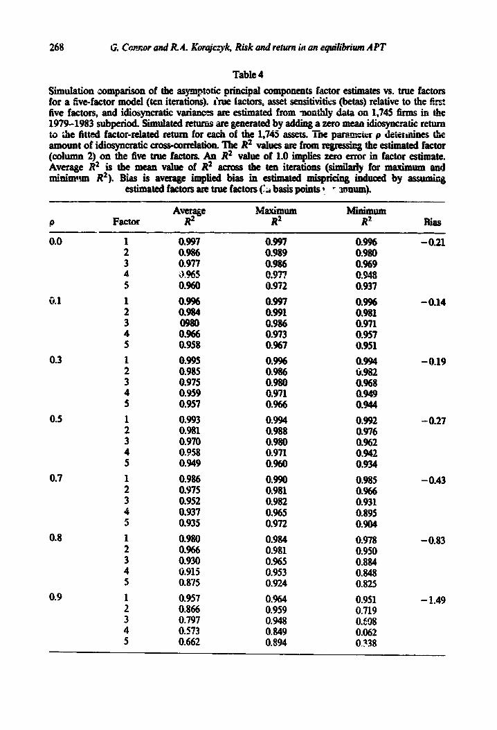
As Theorem 1 indicates, the asymptotic principal components &mates converge to a transformation of the factors, PF, as n approaches infinity. Obviously, it is useful to determine actti number of securities used here is sufikiently large that we can ore the estimation error, *m = G” - LX To do this we present simulation results of asset return series that conform to an approximate factor mdel, estimate the pervasive factors by asymptotic principal components, and compare the factor estimates with the ‘ true’ factors.
We use the fkst five estimated factors obtained from the 19794983 sub- period as the ‘true’ factors, F (F is a 5 x 60 matrix). The estimates of each asset’s sensitivity to the factors and idiosyncratic variant are obtained from ordimuy least squares (OLS) regretdons of assets’ s ret on the factors. L& B denote the 1745 X 5 factor sensitivity matrix Thr= nondivers& able component of asset returns is given by BF. Idiosyncratic returns are constructed to be temporally independent but possibly cross-sectionahy de- pendent. The idiosyncratic return for asset i in period t is constructed as
e it = Pi-l,, + qi*9 i=2,...,1745,
where qit is a random drawing from a normal distribution with zero mean and a variance chosen so that uf = Var(Zig) is equal t0 the MhIWed idiosyncratic risks from the first-stagz OTC regressions and 0 s p < 1. The value of p deteknes the amount of nonfactor cross-sectionall correlation iz the sample. A value of p = 0 corresponds to the strict factor model studied originally by Ross (1976). One can show that
which is finite as long as p < 1 and the individual idiosyncratic variances are bounded. Thus the correlation structure corresponds to an approximate factor model as defined by Chamberlain and Rothschild (1983). Our asset return matrix is given by BF+ e, where e is the 1745 x 60 matrix of residuals constructed in the above manner. Factor estimaies for each iteration are given by the fhst five eigenvectors of D = R’R/n. We compare these factor estimates with the ‘true’ factors by ex amining the R* values from the regression of each estimate on the five true factors. If there were no rotational indeterminacy we
268 G. Cmm.w and R 4. Korajczy~ Risk and return iti 431 q&btium APT
Table 4
sisnulation comparison of the asymptotic principal components f&or estimates vs. true factors for a five-factor model (ten iterations). hue iactors, asset sensitivities (betas) relative to the first five factors, and idiosyncratic variances are es from -nontMy data on 1,745 fhs in the 1979-1983 subperiod. Simulated wturns are generated by adding a zero mean idiosyncratic return to he fitted factowelated return for each of the 1,745 assets. Xhe pararnete:r p deteh&.nes the amount of idiosyncratic crossc0 rrelation The R* v&es are from qresshg the estimated factor (column 2) on the five true factors. An R* value of 1.0 implies zero error in factor estimte. Average R2 is the mean value of R* moss the rnhimun R*). Bias is average implied k&u in
estimated factors am true factors (d
P Factor AVCIlh!ge
R2
0.0 1 2 3 4 5
il.1
0.3
0.5
0.7
0.8
0.9
1 2 3 4 5
1 2 3 4 5
1 2 3 4 5
0.997 0.986 0.977
0.997 o-9%9 0.986
,977 0.972
0.9% - 0.21 0.980 0.%9
0.960 0.937
0.9% 0.984
0.966 0.958
0.997 0.991 0.986 0.973 0.%7
0.996 0.981 0.971 0.957 0.951
0.995 0.996 0.994 0.985 0.986 li.982 0.975 0.980 0.968 0.959 0.971 0.949 0.957 0.966 0.944
0.993 0.994 0.992 0.981 0.988 0.976 0.970 0.980 0.962 0.958 0.971 0.942 0.949 0.960 0.934
0.986 0.990 0.985 0.975 0.981 0.966 0.952 0.982 0.931 0.937 0.965 0.895 0.935 0.972 0.904
0.980 0.984 0.978 0.966 0.981 0.950 0.930 0.965 0.884 0.315 0.953 0.848 0.875 0.924 0.825
0.957 0.964 0.951 0.866 0.959 0.719 0.797 0.948 O./O8 0.573 0.849 0.062 0.662 0.894 0.138
- 0.14
- 0.19
- 0.27
- 0.43
- 0.83
- 1.49
first true factor.
for factors 4 and 5. A value of p = 0.9
4. Testresulcs
In this section we test the restrictions implied by five-factor and ten-factor versions of the APT, we also test the CAP tsing equal-weighted and v&x-weighted indices. The pricing themy of section 2 imposes a testable cross-equation restriction on the parameters of a m3hhmriate regression of asset excess returns on the factors. Let an be the vector of intercepts in a regression of R” oh the factors
R” = aneT’ +- B”F+ en, OQ)
270 6. Connor ad RR. Kwajczyk, Risk and return in an eqdibrium APT
in ui (as I’+ 60) implied by this EIV problem is given by
pliIll(a^i-Qi)= 0 (10 y’LnrLnv) -‘y’LntQ;bi, T+m
where Qq is the k x k c~vtiance matrix of factor estimation errors ( bi is the k X 1 vector of factor sensitivities of asset i. The last column of table 4gkses ks of the average bias in our simulations across the 1,745 assets. The average bias is expressed in basis points per annum (i.e., an entry of 1.0 represents an average bias of one hundredth of P per year). Our estimates of bias are extremely smA in relation to the es error of q. Thus, we conclude that any rejection of the models tested below is not &My to be due solely zfi &e use of the estimated factors, G”, rather than the true facto- F,
We test for no mispricing (an = 0) against a general &emative hypothesis (a’# 0) as well as some specific alternate hypotheses for size-reIated and seasonal eff=ts. In addition to (lo), we estimate the mode& which
of January to d.ifKer Z-am mispricing (1983)]:
where DJ is a F-ve!ctor that takes on the value of unity during January and zero elsewhere. The theory implies that a;Lv = a; = 0 where a& (a;) repre- sents the non-January (January) specific mispricing.
If asset returns follow a strict factor model in which idiosyncratic returns are independent across assets (i.e., VR is diagonal) then joint tests or” Q” = O would be relatively straightforward. In this case one would only need the estimates of ai and the individual standard errors of the estimates. However, if asset returns foIIow enIy an approximate factor model (V” nondiagonaI with bounded eigenvalues as nr + CD), we also need to calculate the covariances of iii and &j for i +j. ithout prior restrictions, this requires the estimation and inversion of the full n x n covariance matrix Pa. This is not feasible in our case, since n is between 1,487 and 1,745.
V/e use two approaches to overcome this problem. F&i, we group securities into portfolios on the basis of Grm size, which has shown ability to predict deviations from the CAPM priciig relation, and test the hypothesis that the portfoIio abnormaI returns are zero. Such a grouping procedure, however, may mask important deviations from the modei if the deviations are unrelated to the instruments us to assign assets into portfolios.
Because of the potential masking of pricing errors, we also test the model by estimating misprictig for each inciividual security. Tests of Jcint hypotheses about mispricing across assets are made feasible by the assumption that F” is block=diagonal ywhere the blocks are determ&d by three-digit SIC codes. That
. G. Cormor and RA. Korajmyk, Risk ad return in an equilibriwn AFT
is, fkms in different three-digit industries are assumed to have idiosyncratic returns.
We present the resuhs for the grouped portfokx first and the disaggre@d
results later. Iln each subperiod we rank the se~uritks with no missing
observations by firm size and form ten portfolios. We define sk as the market value 0 for the December 1963). The from the smalfest size decikg and so on. The ten time-series regessions of (10) [or of (ll)] fit into a standard multivaCate The restric- tions that uJ@=O (or u$~=~$=O) can be arge-sample tests [e.g., Wald, likelihood ratio (LR), and multiplier (LM) tests].
asymptotkaUy, they may give confIicting and Savk (1977)]. In applications quite
&m&r to ours S 1982) shows that both the Wald and LR tests have pronounced tendencies to reject too often. Because of these problems the test statistics we report m mod&d vezsions of the LR test that are suggested in Rao (1973, pp. 554~556)! The statistic is given by
where I prl(l PJ) is the deterknant of tie maximum likelihood estimate of the error covariance matrix from the regression in its restricted (unrestricted) form, T is the number of time series observations, It: is the number of factors, and p is the number of cross-sections in the multivariate regression. For the hypotheses tested kx, ARao (1973) shows that the statistic has (under the assumption of normally distribu+A errors) an exact small-sample distribution, which is F(p, T- k -p). The statistic in (12) is identical to the statistic described on page 32 of Gibbons, Ross, and Shanken (1986). The use of this statistic or ones similarly adjusted for small samples can lead to quite difkrent inferences from the usual largesample test statistics [see inder (‘5985) ad Shanken (1985a)].
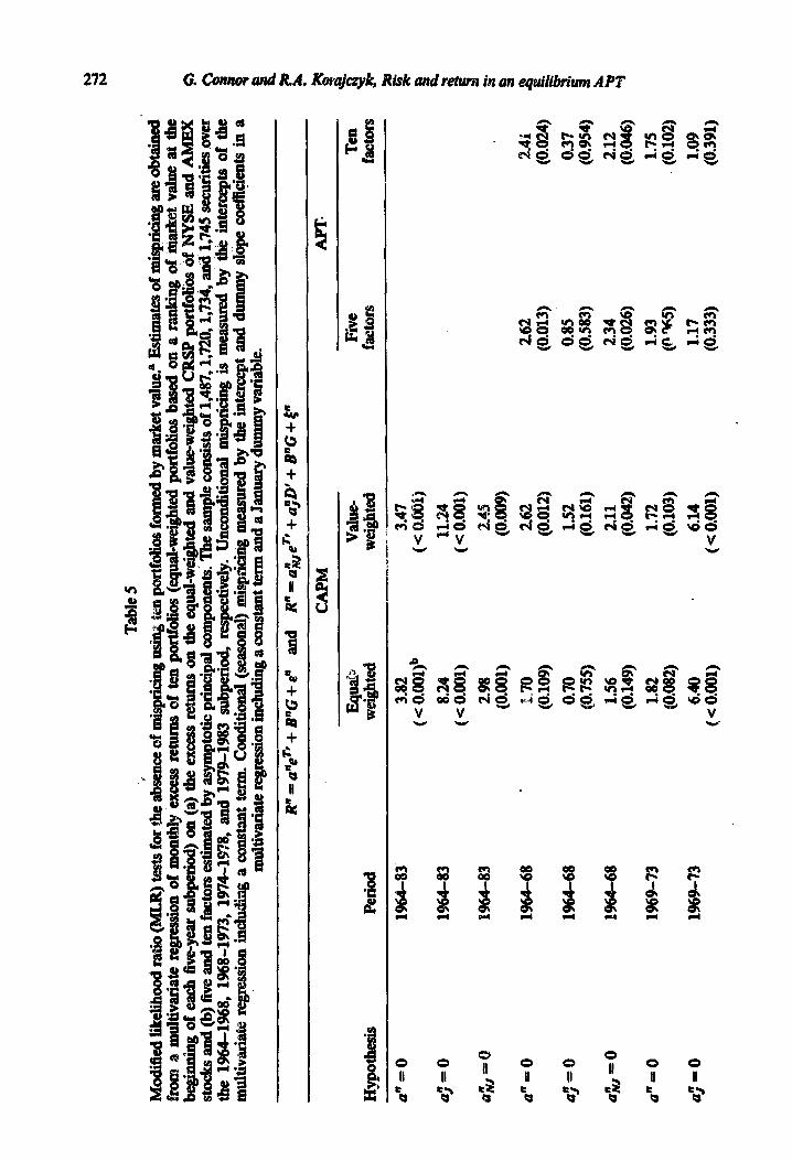
Table 5 gives the results of our tests of ‘&s pG.ug restrictions for the ten size-based portfolios. The APT does better (a lower frequency of reiections) than the CAPM in explaining ary seasonality in a;! = Q). At first glance, the APT to do a worse job of e nonseasonal mispricing (a;tr = 0). Looking at rejection fates =m= non- nested models can be misleading, however, better (smaller values of ial) may be rejected if the deviations more precisely (i.e., the test has more power).
*We have also calculated ople standard versions of the Wald and LR statistics.
Tab
le 5
Mod
&d
likel
ihoo
d ra
tio
(ML
R) t
ests
for
the
abhn
ce o
f m
ispr
icin
g usi
q lm
por
tfol
ios f
orm
ed b
y m
ark
et va
lue?
Est
imat
es o
f m
&ri
cing
ar
e ob
tain
ed’
&om
a m
ulti
vari
ate
regz
es&
on o
f m
onth
ly ix
cess
ret
urns
of
ten
port
folio
s (e
qual
-wei
ghte
d por
tfol
ios
base
d on
a r
ank
@
of <
mar
ket
valu
e at
the
be
ghbg
of
eac
h fi
ve-y
ear s
ubpe
riod
) on
(a)
the
exce
ss r
etur
ns o
n th
e eq
u&w
eigh
ted
and
vahe
-wei
ghte
d C
RS
P p
ortf
olio
s of
NY
SE
and
AM
EX
st
ock
s an
d (b
) fi
ve a
nd t
en f
acto
rs es
tim
ated
by
asym
ptot
ic p
rinc
ipal
com
pone
nts:
The
sam
ple
cons
ists
of
1,48
7,1,
720,
1,73
& a
nd 1
,745
secu
riti
es o
ver
the
1964
-1%
8,
1968
-197
3, 1
97~
W?8
, an
d 19
79-1
983
subp
erio
d, r
espe
ctiv
ely.
Unc
ondi
tion
al m
ispr
icin
g is
mea
sure
d by
the
int
erce
pts
of t
he
xuti
tiva
riat
e re
ggon
in
clud
ing
a co
nsta
ut t
erm
. Con
diti
onal
(se
ason
al) m
ispr
itig
m
easu
red
by t
he i
nter
cept
and
dum
my
shpe
coe
ffi@
nts
in a
m
ulti
vari
ate r
egre
ssio
n inc
ludi
ng a
con
stan
t ter
m a
ud a
Jan
uary
dum
my
vari
able
.
Rn=
aneT
t+B
nG+
em
and
Rn=a;lrreTf+ajD'+BnG+~n
Hyp
othe
sis
Per
iod
mu&
w
eigh
ted
CA
PM
A
Fr
Val
w-
Fiv
e T
en
Wei
gBte
d fa
ctor
s fa
ctor
s
a"=0
a; =0
a$p=Q
a"=0
a;= 0
a;,=0
a" =0
a;=
0
1964
-83
1964
-83
1964
-83
1964
-68
1964
-68
1964
-68
1969
-73
1969
-73
3.82
3.
47
( < O
.oO
l)b
( < O
.O0l
j
8.24
11
:24
( < 0
.001
) (<
0.0
01)
2.98
2.
4§
(0.0
01)
(O-0
09)
E-7
0 2.
62
(0.1
09)
(0.0
12)
0.70
1.
52
(0.7
55)
(0.1
61)
1.56
2.
11
(0.1
49)
(OB
42)
1.82
1.
72
(0.0
82)
(0.1
03)
6.40
6.
14
( < O
.o(b
l)
(S 0
.001
)
2.62
(0
.013
)
0.85
(0
.583
)
2.34
(0
.026
)
1.93
(P
W
1.17
(0
.333
)
2.41
(0
.024
)
0.37
(0
.954
)
2.12
(O
-046
) 1.
75
(0.1
02)
1.09
(0
.391
)

a;,=
0
an=0
aJ"=
O
as-=
0
an=0
a;=
0
0.85
(0
.588
)
2.0
2
(0.0
56)
3.5
3
(0.0
02)
2.0
2
(0.0
57)
1.8
4
(0.0
85)
0.6
3
(0.7
80)
a$,=
0 1.7
3
(0.1
08)
an=0
70.9
9
(0.0
02)
a;=0
48.3
7
(0.1
71)
a&-O
60.5
6
(0.0
19)
‘Ind
epen
dent
vari
able
s are
the C
RSP
stoc
k por
tfol
ios o
r fa
ctor
esti
mat
es pr
oduc
ed b
y th
e as
ympt
otic
pri
ncip
al co
mpo
nent
s tech
niqu
e, G
, a v
ecto
r of
ones
, eT
, and
a d
umm
y var
iabl
e f6r
hnu
ary,
D,, A
vera
ge n
&pr
icin
g is
mea
sure
d by
a”,
hw
ary-
spec
ific
m
ispr
icin
g by
a$
and
non-
kum
ary~
spec
ific
m
ispr
icin
g by
a;,
. (D
F,)
= 10
. For
the
Tes
t sta
tist
ics a
re th
e m
odif
kd L
R t
est
[see
Rao
(19
73, p
. S
SS
)] w
hich
has
an
F d
istr
ibut
ion.
Num
erat
or de
gree
s of
free
dom
19
6443
pe
riod
den
omin
ator
deg
rees
of
free
dom
(De)
is
equ
al to
22
9 (a
) an
d 22
8 (a
, an
d a,
):
For
eac
h su
bper
iod D
e is
eq
ti
to
49
(C
XP
M:
a),
48 (
CA
PM
: aJ
and
+,,)
, 45
(/@
T-k
a),
44
(AP
T-s
: aJ
and
uN,)
, 40
(AP
T-1
0: a)
, an
d 39
(APT
-10:
aJ
and
a&.
-
b,w
4tlu
es in
par
enth
ews.
C
d Agg
rega
tion
of
subp
erio
d re
sult
s.. S
tatk
tic h
as x
2 di
stri
buti
on, a
sym
ptot
ical
ly, w
ith
40 d
egre
es o
f fr
eedo
m u
nder
the
nul
l hy
poth
esis
.
1969-7
3
1974-7
8
1974-7
8
197G
78
1979-8
3
1979-8
3
1979-8
3
Agg
rega
ted=
Agg
rega
ted
Agg
rega
ted
1.8
4
(0.0
78)
0.8
3
(0.6
01)
3.5
3
(0.0
01)
0.6
4
(0.7
70)
0.9
5
(0.4
95)
2.6
6
(0.0
11)
0.7
8
(0.6
49)
50.0
6
(0.1
32)
102.1
7
( < 0
.001)
45.7
0
(0.2
42)
2.1
1
(0.0
42)
1.1
3
(0.3
61)
5.9
9
( < 0
.001)
0.7
1
(0.7
11)
1.1
3
(0.3
58)
2.9
9
(0.0
05)
0.8
1
(0.6
18)
60.4
4
(0.0
20)
123.7
1
( < 0
.001)
52.9
9
(O.s
sz)
1.0
7
(0.4
08)
1.7
3
(0.1
03)
1.9
7
(0.0
61)
1.7
4
(0.1
03)
1.7
4
(0.1
00)
0.8
7
(0.5
71)
1,8
1
(0.0
87)
71.6
3
(0.0
02)
46.0
5
(0.2
36)
63.1
9
(0.0
11)
274 G. Connor and I&A. Korajczyk, Risk and return in an equGb&m APT
A closer look at the parameter estimates gives a very different picture of the relative p&ommce of the models than does a casual investigation of the test statistics in table 5. Fig. 1 plots the average mispricing (across the four s&p&&) for each size portfolio in relation to the CAPM (using the value-weighted and equal-weighted portfolios of NYSE and AMEX stocks) and the APT with five factors. The vertical axis is the average value of ui for each size portfolio from smallest ($1) to largest (SlO). Although the aggregate statistics reported in table 5 indicate a stronger rejection of an = 0 for the APT &a for the equal-weighted and value-weighted CAPM, the actual value of AFT mispricin~ is much smaller (for all but one portfolio) in relation to the value-weighted CAPM and slightly smaller (for all but two portfolios) in relation to the equal-weighted CAPM. Thus, the stronger rejection of the five-factor APT is due to more precision in the estimates of ai (i.e., R* values around 0.98 versus 0.75) rather than larger pricing errors.
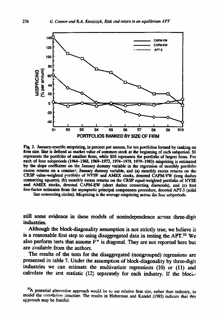
Fig. 2 presents some of tht: most interesting results. One of the most persistent empirical anomalies in asset pricing has been that the common equity of small firms earns a much higher (risk-adjusted) return than the equity of large firms, particularly in January. The results in fig. 2 indicate that, when we use the fivefactor APT to adjust for risk there is no relation between January-specific mispricing and firm size. Also, although the APT does not totally explain the non=1 ,anuary specific size effect (see fig. 3), it does at least as well as the versions of the CAPM. Again, this is quite different from what one might guess from the statistics in table 5. The nature of the factor-model approach (in which the factor estimates are chosen io eqdah variation) would lead one to expect the APT might do better in explaining a time-varying size anomaly. It is encouraging, at least, that the evidence is consistent with a model in which the anomalous CAPM January seasonal effect is due to assets’ different risks relative to factors with seasonal risk premiums. Work along the lines of Chen, Roll, and Ross (1986) may help us identify the nature of these seasonal factors.
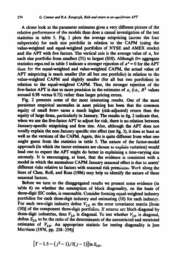
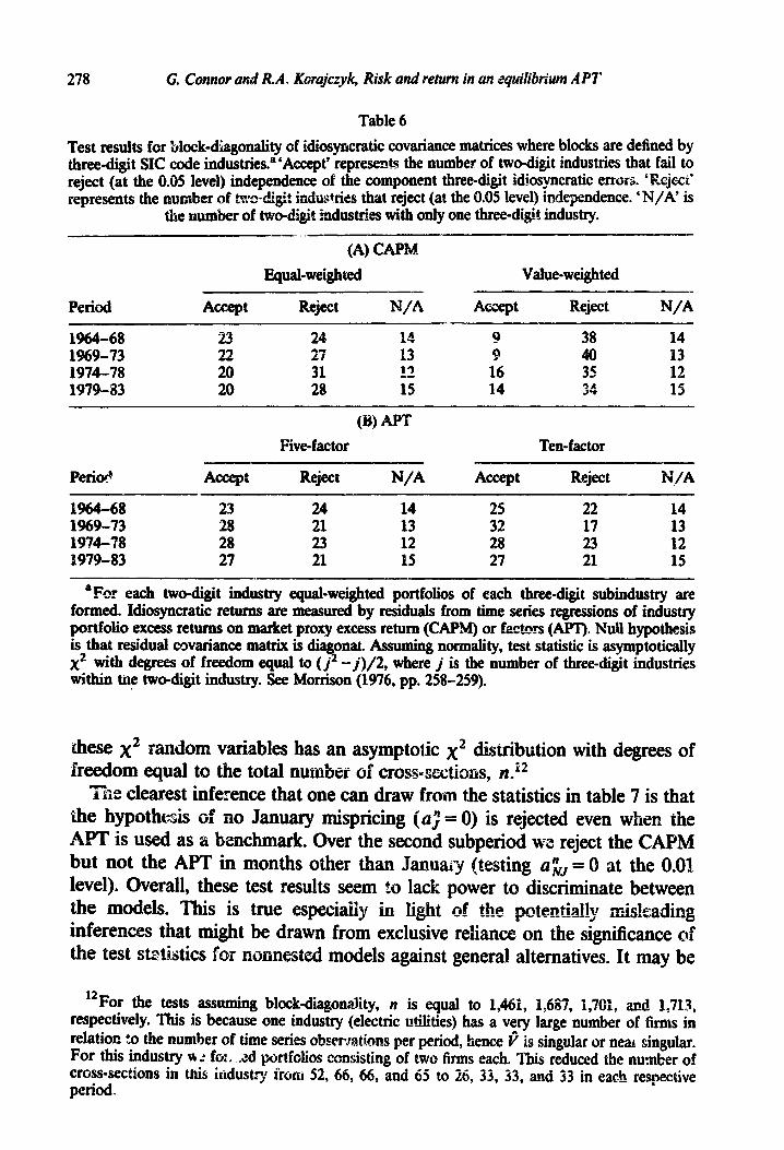
Before we turn to the d&aggregated results we present some evidence (in table 6) on whether the assumption of block diagonality, on the basis of three-digit SIC codes, is reasonable. Consider forming equal-weighted industry portfolios for each three-digit industry and estimating (10) for each industry. For each two-digit industry define Vzo as the error covariance matrix [from (lo)] of the component three-digit portfolios. If returns are block-diagonal by three-digit industries, then VzD is diagonal. To test whether V2D is diagonal, define szD to be the ratio of the determinants of the unrestricted and restricted estimates of VzD. An appropriate statistic for testing diagonality is [see Morrison (1976, pp. 258-25911

G. Connor and RA. &uajczyk, Risk and return in an equibiwn APT
10 -- CAPM-VW
16
275
s3 s4 s!i s6 ST s0
PORTFOLIOS RANKED BY SIZE OF FIRM
Fig. 1. Mispricing, in percent per annum, for ten portfolios formed by ranking on firm size. Size is defined as market value of common stock at the beginn& of each subperiod. Sl represents the portfolio of smallest firms whiIe SlO represents the portfolio of largest Grms. For each of four subpA.xIs (19661%8,1%9-1973,197~1978,1979-1983) mispricing is estimati By the inter- cept in the ~~ression of monthly portfolio excess returns on a constant, and (a) monthly exm returns on the CRSF valwweighted potiolio of NYSE and AMEX stocks, denoted CAPM-VW (long dashes -=cting qua=), (b) -My excess saims on the CR!5P equal-weighted portfolio of NYSE and AMEX stocks, denoted CAPM-EW (short dashes connecting diamonds), and (c) firs: five-factor estimates from the asymptotic principal components procedure, denoted APT-5 (solid line connecting circles). Mispricing is the average mispricing across the four
subperiods.
which, assuming normality, has an asymptotic distribution that is x2 with degrees of freedom equal to (j* -. j>/2, where j is the number of three-digit industries in the particular two-digit industry. Table 6 shows the number of iiriio-digit industries that accept and reject the null at the 0.05 level. The industries marked N/A are those with only one three-digit industry within the two-digit classification.9
The results for the CAPM, especially using the value-weighted market portfoho, show a relatively large number of rejtitions. The five- and ten-factor models show less evidence against the block-diagonality assumption. There is
‘These tests will tend to reject independence too oftca if security returns have probability distributions with larger kurtosis than the normal distribution [see Muirhead (1982, pa 547)]. Given the evidence of ‘fat tails’ in return distributions, L - . . *L= -4ence against independence is not as strong as a literal interpretation of the numbers in table 6 sould indicate.
276 G* Cmnor end R.A. Komiczyk, Risk and return in an equilibrium APT
5 I I I I I I I I _ - _
Sl s? s3 s4 St5 !s6 s7 s8 s9 SlO
PORTFOLIOS RANKED BY SIZE OF FIRM
Fig. 2. January-specific mispricing, in percent per annum, for ten portfolios formed by ranking on firm size. Size is defined as market value of common stock at the beginning of each subperiod. Sl represents the portfolio of smallest firms, while SlO represents the portfolio of largest firms. For each of four subperiods (19644%8,1%9-1973,197~1978,1979-1983) m&pricing is estimated by the slope coefficient on the January dummy variable in the regression of monthly portfolio excess returns on a constant, January dummy variable, and (a) monthly excess returns on the CRSP value-weighted prHo!/io of NOSE md AMEX stocks, denoted CAPMJW (long dashes connecting squares), (b) monthly excess returns on the CRSP equal-weighted portfolio of NYSE and AMEX stocks, denoted CAPM~EW (short dashes connecting diamonds), and (c) first five-factor estimates from the asymptotic principal components procedure, denoted APT4
line connecting circles). M&pricing is the average mispricing acroti the four subperiods. (solid
still some evidence in these models of nonindependence across three-digit _ industries.
Although the block-diagonality assumption is not strictly true, we believe it is a reasonable first step to using disaggregated data in testing the APT.1o We also perform tests that assume Vn is diagonal. They are not reported here but are available from the authors.
The results of the tests for the disaggregated (nongrouped) regressions are presented in table 7. Under the assumption of block-diagonality industries we can estimate the multivariate regressions (10)
by three-digit or (11) and
calculate the test statistic (12) separately for each industry. if the blo&-
“A potential alterr4ve approach would be to aose relative firm size, rather model the coar&?ticn structure. The results in approach may be fruitful.
I than industry, to indicate tha! this

G. Connor and R.A. Korajczyk, Risk and return in an equilibrium APT 271
Sl s2 s3 s4 Sf s6 S? s6 s9 SlO
PORTFOLIOS RANMEU Wt’ SE GF FIRM
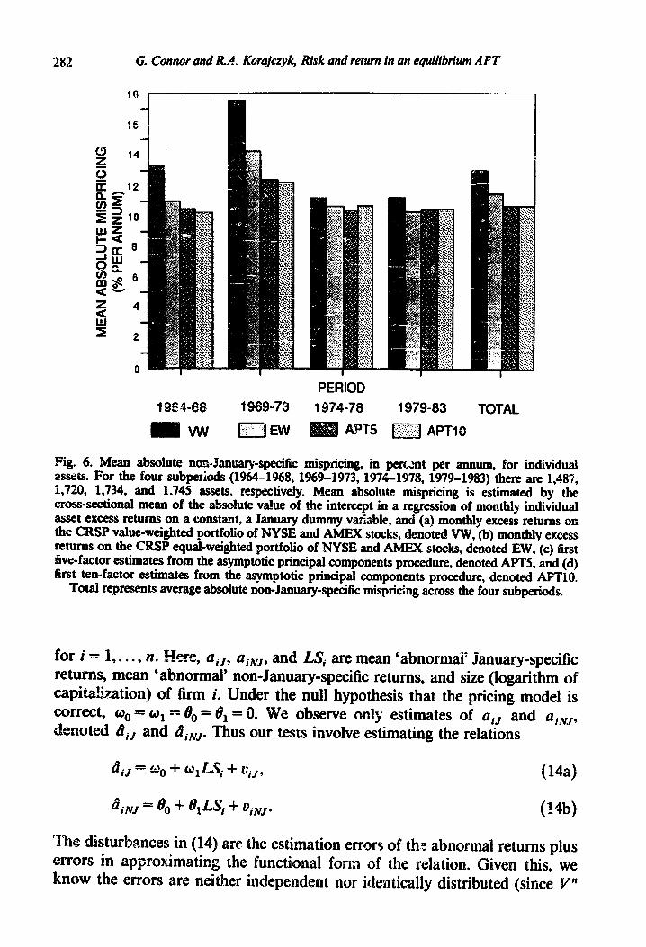
Fig. 3. Non&m3ry~specific mispricing, in percent per annum, for ten portfoiios formed by ranking on fmn size. Size is defined as market value of common stock at the beginning of each subperiad. 411 represents the portfolio of smallest firms, while SfO represents the portfolio of largest firms. For each of four sub~&xis (H&4-1%8, 1969-1973, 1974-1978, 1979-1983) mispricing is &nated by the intercept in the regression of monthly portfolio excess returns on a constant, Januatt dummy variab , 2x~i.i (a) monthly excess returns on the CMP va!ue+veighted portfolio of NYSE r?d AMEX stocks, denoted CAPM-VW (long dashes connecting squares), (b) monthly exess returns OE the CRSP equakweighted portM~ of NYSE aud AMEX stocks, denoted CAP&EW (short dashes connecting diamonds), and (c) first five-factor estimates from the asymptotic principal components proced-ure, denoted APT-5 (solid line connecting circles).
Misprking is the average mispr&g across the four subperiods.
diagonality assumption is true, these F statistics are independent across blocks. However, unlike for x2 random variables, we cannot aggregate across b!o& bj simply summing the test statistics. We use an aggregation procedure similar to the one suggested, in a, slightly different context, by Sh (1985a).” We approximate each F statistic by a xi distribution with th tail area, where p is the number of cross-sections in the block. e sum of
“Shanken (1985a) suggests approximating the F statistic by a at4jrmJ distribution. That is, firid the v&e of a unit normal with the same tail area (p-value) as the computed F statistic. The sum of l &ese -tit normals, divided by the square root of the number of blocks, has a unit normal distribtt tion. Qur application different in that we
different degrees of use of the nor
_*_I.. WCi&iiE GE W&W VB’CIV~ pla h kln& rmbmdl~cc nf ci7p T&c Jo_ nnt a hwwwrn fnr tpctc ;* c~~~L~.. II not.-\
*“~zu”aw”Y Y_ e-M. _.l” _Y WY. “.*a.-. l . ax?. .WYIU ..a USIQIsAbU \11703aj*
since the F statistics in that study have the same degrees of freedom.
218 G. Connor ami R.A. Korajczyk, Risk and return in an quilibrium API
Table 6
Test results for block-&agonality of idiosyncratic covariance matrices where blocks are defined by threedigit SIC code industries.a ‘Accept’ represents the number of two-digit industries that fail to reject (at the 0.05 level) independence of the component three-digit idiosyncratic errors. ‘Rejee:’ represents the number of Tao-digit industries that reject (at the 0.05 level) independence. ‘M/A’ is
the number of two-digit industries with only one three-digit industry. -- _
(A) CAPM
Equal-weighted Value-weighted
Period Accept Reject WA Accept Reject WA
1964-68 23 24 1A 9 38 14 1969-73 22 27 ;‘; 9 40 13 1974-78 20 31 12 16 35 12 1979-83 20 28 15 14 34 1c 13
(W APT Pive-factor Ten-factor
Period A-Pt Reject WA Accept Reject N./A
1964-68 23 24 14 25 22 14 1969-73 28 21 13 32 17 13 19?4-78 28 23 12 28 23 12 1979-83 27 21 15 27 21 15
aFor each two-digit industry equal-weighted portfolios of each three-digit subindustry are formed. Idiosyncratic returns are measured by residuals from time series regressions of industry portfolio excess returns on market proxy excess return (CAPM) or factors (APT). Null hypothesis is that residual covariance matrix is diagonal. Assuming normality, test statistic is asymptoticahy x2 with degrees of freedom equal to (j* - j)/2, where j is the number of three-digit industries within the two-digit industry. See Morrison (1976, pp. 258-259).
these x2 random variables has an asymptotic x2 distribution with degrees of freedom equal to the total number of cross-sections, n.l*
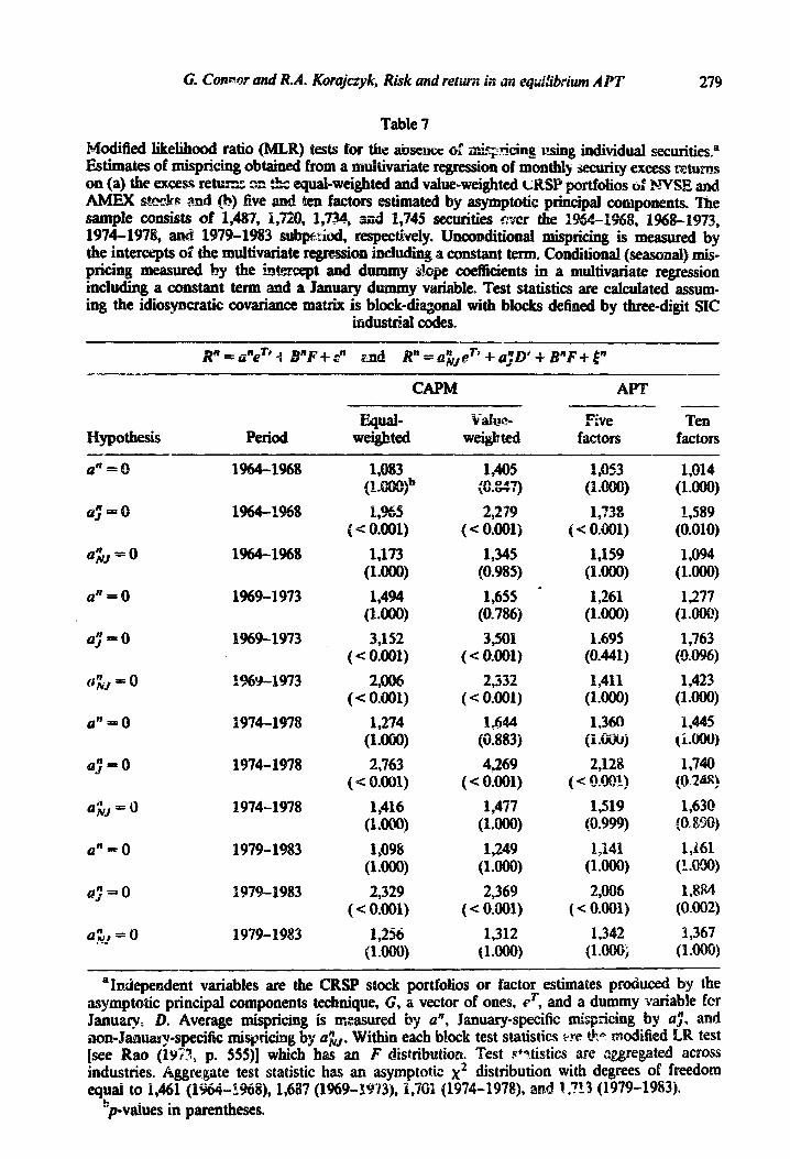
The cle&est inference that one can draw from the statistics in table 7 is that the hypoth&s of no January n&pricing (a; = 0) is rejected even when the APT is used as a benchmark. Over the second subperiod wc reject the CAPM but not the APT in months other than Janua&zy (testing u;CrJ = 0 at the 0.01 level). Overall, these test results seem to lack power to discriminate between the models. This is true especitiy in tight of the potentia!;ly Lmisleading inferences that might be drawn from exclusive reliance on the significance of the test statistics for nonnested models against general alternatives. It may be
I2 For the tests assuming block-diagonality, n is equal to l&i, i,687, i ,761 p and 1,713 i respectively. This is because one industry (electric utilities) has a very large number of firms in relation $0 the number of time series observations per period, hence t is singular or ne;u singular. For this industry a : fen. ..zd portfolios consisting of two firms each. This reduced the number of cross-sections in ttis industry from 52, 66, 66, and 65 to 26, 33, 33, and 33 in each respective period
G. Conmr and R.A. Korajczyk, Risk and reium is; m eq&britun APT 279
Table 7
Modified IikeIihood ratio (MLR) tests for the absmcc CS tiqtitiq wing individuaI secwities.a Estimates of mispticing obtained from a multivariate regression of monthly wurity excess returns on (a) the excess retuzs on l &c equaLweighted and valw-weighted c;WSP portfolios tif s?SE and AMEX s+&&s and (b) five and ten factors estimated by asymptotic principal components. The sampIe consists of 1,487, 1,720, l,734S and 1,745 securities over the 1964-1968, 1%8-1973, 1974-1978, ancI 1979-1983 subp&tI, respectively. UnconditionaI mispricing is measured by the intercepts of the m&variate regre&on including a constant term. ConditionaI (seasonaIj mis- pricing measured by the ;&rcept and dummy slope coefficients in a muhivariate regression inchuling a constant term and a January dummy variable. Test statistics are calculated assum- ing the idiosyncratic covariance matrix is block=di~onaI with blocks defined by three-digit SIC
industrial codes.
R” = aneT’ f B”F + g? prrd R” = a&pT’ + aJo’ .+ BnF + In
CAPM
I-Iypothesis Period I&p&_
weighted
. Five
factors Ten
factors
aIndependent variables are the CRSP stock portfolios or factor estimates prduced by the asymptotic principal components technique, G, a vector of ones, eT, and a dummy variable for January D. Average n&pricing is measured by Q”, January-specific mispricing by a$ ad non- Janus y-specific mispricing by; +. Within each block test statistics tf_rg *A [see Rao (I!G>; p. SSS)] which h F distribution. Test ,c+?tistics are
re&ate test statistic asymptotic x2 distribution with d equal to i&l (I%&1%8j, i,687 (1969.1Sf3), 1,701 (I974-1978j, and 1,713 (1979-19832.
Sp-vtiues in parentheses.
a”=0
a: = 0
4;lr/ = 0
a”=0
a,R = 0
a;5;r = 8
a”=0
a;=0
a;lrl = 0
a”=0
a; = 0
n Q#l,r = 0
1964-1968
l-i%8
1964-1968
1969-1973
1969-1973
l%Y-1973
1974-1978
1974-1978
1974-1978
1979-1983
1979-1983
1979-1983
1,083 (i SOOOjb
_ -__ ,Y5
(: bo:, 1,173
(1*9fjQ) 1,494
(l.ooo)
3,152 ( *: 0.001)
2,006 (< 0.01)
1,274 (1.W) 2,763
( < O.oOl)
1,416 (l.Oj
1,09& (l.ooo)
2,329 ( < 0.001)
1,256 (l.OOOj
1,405 (0.847)
2,279 ( < 0.001)
1,345 (8.985)
1,655 - (0.786)
3,501 ( < 0.001)
2,332 (< 0.001)
i,644 (0.883)
4,269 ( < 0.001)
1,249 (1 .mj
2,369 (< O.Qol)
1,312 (l*Wj
1,053 (l*~j 17-9
q’-IU
( < 0.i.m)
1,159 (l.Oj
1,261 (l.tj9fIj 1.695
(0.441)
1,411 (l.ooo) 1,360
(l.GGuj
2,128 ( c O_Q@)
1,519’ (0.999)
l,i41 (l.(-joj
2 ( < O.OOlj
1,342 (l.ONjj
1,014 (l.ooo) 1,589
(0.010)
1,094 (l.ooo)
1,277 (Looes)
1,763 (9.0%)
1,423 (l.~j 1,445
(I.000)
1,740 (0 24srj
1,63@ (Q.V%)
1,161 (1.0)
1,884 (0.002)
1,367 (1-W)
280 G. Connor and R.A. Korajczyk Risk and return in an equilibrium APT
1964-68 1969-73
WV r--J Ew
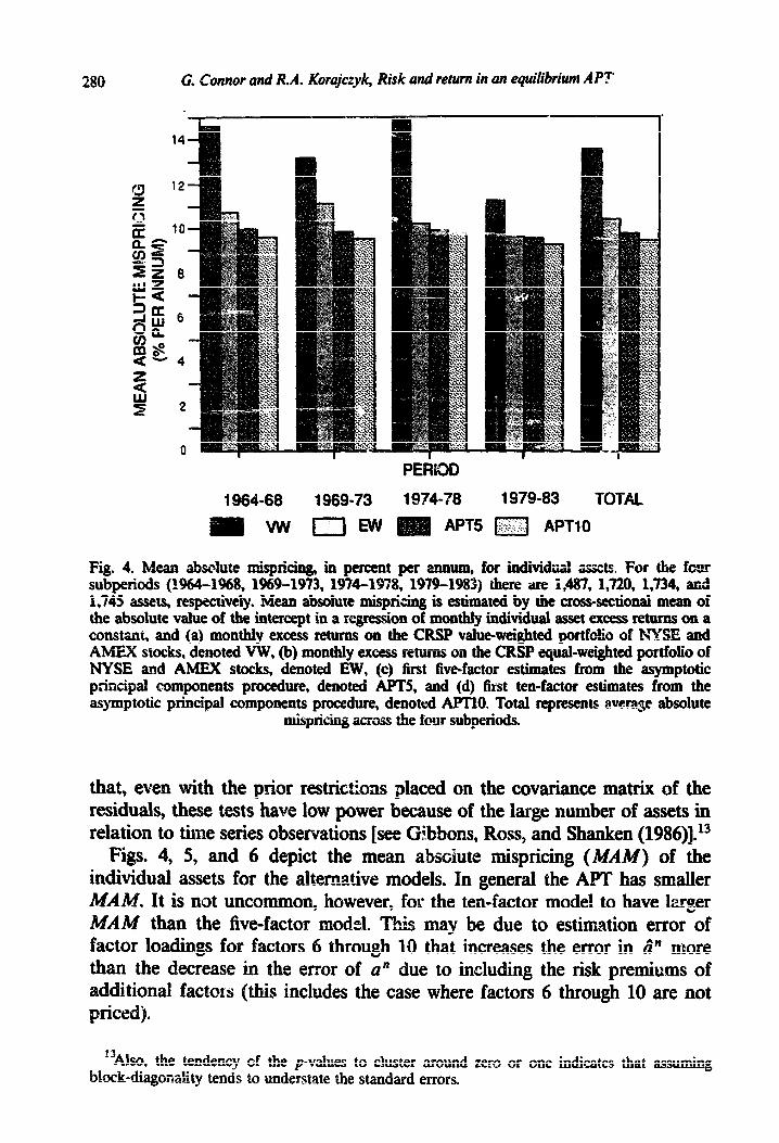
Fig. 4. Mea abs&te ricing, in percent
PERIOD
19740T8 1979-83 TOTAL
APT5 rsj APT10
per annum, for individual assets. For the fovur subperiods (E&4-1%8, 1969-1973, 1974-1978, 1979-1983) there are i&7, 1,720, 1,734, and 1,745 assets, respectively. Mean absolute mispricing is estimated by the cross-sectional mean of the absolute value of the intercept in a qression of monthly individual asset excess returns ou a constat, and (a) monthly excess returns on the CRSP value-weighted portfotic of &TSE and Alex stocks, denoted VW, @) monthly excess returus on the CRSP equal-weighted pmtfolio of NYSE and AMEX stocks, denoted EW, (c) first five-factor estimates from the asymptotic prirzcipal components procedure, denoted APT5, and (d) first ten-factor estimates from the asymptotic principal components procedure, denokd APTlO. Total represents average absolute
misprichg across the four subperiods.
that, even with the prior restrictions @aced on the covariance matrix of the residuals, these tests have low power because of the large number of assets in relation to time series observations [see Gibbons, Ross, and Shanken (1986)].i3
Figs. 4, 5, and 6 depict the mean absolute mispricing (MAM) of the individual assets for the alte_rnative models. In general the APT has smaller
It is not uncommon, however, for the ten-factor model to have larger MAM than the five-factor model. This mav be due to estimation error of factor loadings for factors 6 through 10 that increases the error in a^” more than the decrease in the error of a” due to including the risk premiums of additional factors (this includes the case where factors 6 through 10 are not priced).
“Also, the tendency of the p-values to cluster around zero or one indicates that assuming block-diagmaby tends to understate the standard errors.
G. Connor and R.A. Korajczyk, Risk ad retm in an eqtdibrium APT 281
PERIOD
1964-68 1969-73 1974-78 1979-83 TOTAL
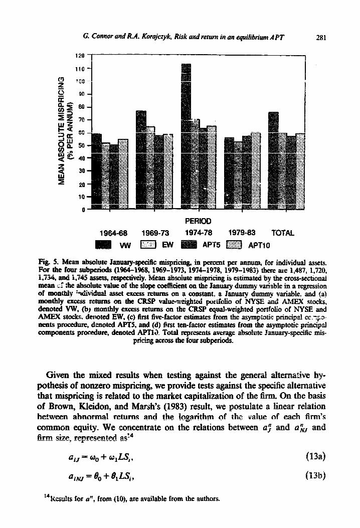
Fig. 5. Mean absolute hwaryqecific mispricing, in percent per annum, for individual assets. For the four subperiods (1%4-l%& l%!?-l!J73,1974-1978,1979-1983) there ate l&37,1,720, 1,734, and 1,745 assets, reqectively. Mean absolute mispricing is estimated by the cross-sectional mean cI the absolute value of the slope coeficient on the January dummy variable in a regression of montMy +Ii~<dual asset excess returns on a constant, a January dummy variable, and (a) monthly excess returns on the CRSP vahe=wi&tt portfolio of NYSE ad AMEX stocks, denoted VW, (b, monthly excess returns on the CRSP equal-weighted portfolio of NYSE and AMEX stocks. denoted EW, (c) first five-factor estimates from the asympiotic principal cc.:p+ nents procedure, denoted APTS, and (d) first ten-factor estimates from the asymptotic principal components procedure, denoted APT&& Total represeuts average absolute January-specific mis-
prkhg across the four subperiods.
Given the mixed results when testing against the pothesis of nonzero m&pricing, we provide tests against that m&pricing is related to the market capitalization of Brown, Kleidon, and Marsh’s (1983) result, we between abnormal returns and the logarit of the value of each common equity concentrate on the relations between QJ” firm size, repres
4iJ = 00 + O,LS,?
14Resuhs for a”, from (lo), are available from the authors.
I, I
I_
G. Connor and R.A. Korajczyk, Risk and return in an equilibrium APT 283
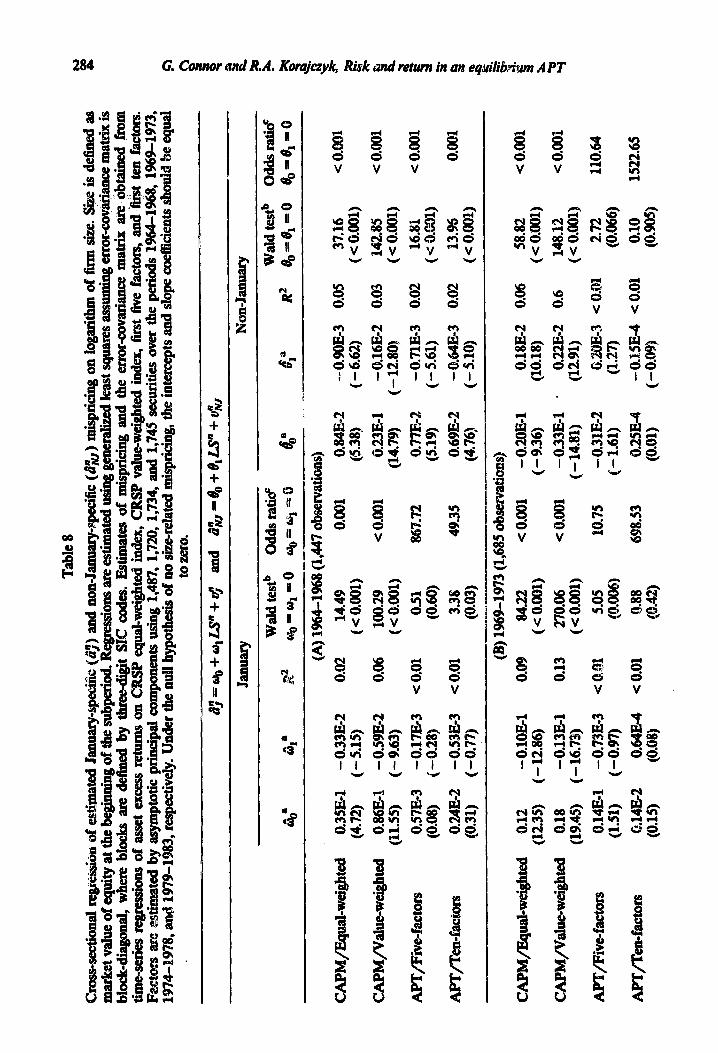
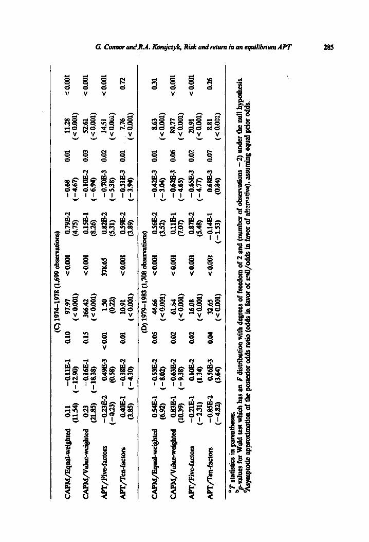
is not a scalar pntrix and the covariance matrix of the t?;‘s is proportional to V”). However, the covariance matrix of the errors can be estimated from the time series residuals from (ll)? e estimate (14) using ordinary least squares (OLS), weighted least squares (WI2Q and generalized least squares (C&S), which correspond to assuming Vn is scalar, diagonal, and block==diagonal, respectively. As before, the blocks are assumed to be defined by three-digit SIC industrial codes. only the results for the block-diagonal case are pre- sented. These are given in table 8. In addition to the piwameter estimates, we show the R2 value, a sam~ti~+i;or?r-based (Wald) test that the coefficients are jointly zero [see (3.3) on p. 313 of Theil (197111, and an asymptotic approximation of the posterior odds ratio for the null assuming equal prior odds.
We report the posterior odds ratio since statistical significance at conven- tional levels (e*g., 05 or 0.01) need not @#y strong evidence against the null hypothesis in very large samples (we have appromately 1,700 observations in the regressions reported in table 8). This is because when we hold the probability of type I error of the test constant, the probability of type II ezr~r goes to zero as the sample size increases. Thus, with large stt.mpies all but trivial deviations from the pricing theory will be rejected at conventional sign&ance levels [this property is sometimes referred to as Lindley’s paradox; see Zellner (1971, pp. 303-3(B)]. The asymptotic approximation of the pos- terior odds ratio, K, for our null hypothesis is a simple function of the F statistic reported in table 8, gives by S%
(1%
where n is the Bumber of observations and F,. n-2 is the value of the F statistic [see eq. (54) of Rossi (1980)], The dependence of the odds ratio on sample size as well as the F’ statistic is clear from (15).
We first investigate the relation between January-specific abnormal returns and firm size. From a classical sampling&eory point of view the hypothesis that a0 = a1 = 0 is rejected (at anv significance level above 0. instance except for the tern-factor Awni during mcl MY-lY73, an the five-factor APT during 1964-1968 and 197 find the standard negative relation between posterior odds ratio favors the hypothesis of n&pricing in three out of four subperiods for
the inverse of the cross-produ ] - I. Staudaii! results for the
Zellner (1971, p. 24O)j imply that var(cij the constants of tiouality are the (23 the assumption truca’sareli covariance matrices in (14) are proportional to V”.
atrix of the regressors in (11). ~~za+~ R*wssion m
Tab
le 8
Cro
ss-s
ecti
onal
reg
re&
oii
of e
stim
ated
Jan
uary
-spe
&:
(&;)
and
non
&uu
ary+
peci
fic
(a;,
) m
ispr
icin
g on
lo@
thm
of
@rm
size
. sir
a is
def
ined
as
mar
ket
val
ue o
f eq
uity
at
the
beg,
in&
g of
the
subp
erio
d. R
egre
ssio
ns ar
e es
tim
ated
usi
ng g
ener
aliz
ed le
ast s
quar
es a
ssum
ing
erro
r-co
va@
tce
mat
rix
is
bloc
k-d
iago
nal,
whe
re b
lock
s ar
e de
fine
d by
thr
ee&
tit
§IC
cod
es.
Est
imat
es
of m
iqic
ing
and
the
erro
r-co
vari
ance
mat
rix
v ob
tain
ed f
rom
*s
erie
s re
gres
Gon
s of
asse
t ex
cess
ret
urns
on
CR
SP
equ
al-w
eigh
ted
inde
x, C
RS
P v
alue
-wei
ghte
d in
dex,
fir
st f
ive
fact
ors,
and
fir
st t
en f
acto
rs.
Fac
tors
~X
Z atim
ated
by
asy
mpt
otic
pri
ncip
al c
ompo
nent
s us
ing
1,48
7, 1
,720
, 1,7
34, a
nd 1
,745
secu
riti
es o
ver
the
peri
ods
Z&
4-1%
8,
1969
-197
3,
1974
-197
8, m
d 19
79-1
983,
res
pect
ivel
y. U
nder
the
nul
l hyp
othe
sis o
f no
siz
e-re
late
d mis
pric
ing,
the
inte
rcep
ts an
d sl
ope
coef
fici
~ts
sho
tid
?X eq
ual
to z
ero.
Janu
ary
Non
-Jan
uary
Wal
d te
stb
Odd
s rat
i&
Wat
d te
stb
Odd
s ra
ti&
-a
%
ia
la
I32
a?%
q)
‘&y(
) qp
*;r=
fj 6b
” 4
Rf
6),=
9,-o
e,
=e,
-0
-“1-
-. ’
A--
(A
) 19
64-1
%8
(1,4
47 o&
rvat
ions
)
CA
PM/
EC
p&W
@bX
i 0.
35E
-1
- 0.
33E
-2
0.02
14
.49
0.00
1 0.
84E
a2
- 0.
9OE
-3
0.05
37
.16
< o
*ON
(4
.72)
(-
5.15
) ( <
0.0
01)
(5.3
8)
(-6.
62)
( < 0
.001
)
CA
PM
/Val
ue-w
eigh
ted
0.86
E-1
-
0.59
E-2
0.
06
100.
29
< 0
.001
0.
23E
-1
- O
.l6E
-2
0.03
14
2.85
<
0.0
01
(11.
55)
(-9.
63)
( < 0
.001
) (1
4.79
) ( -
12.
80)
( ( 0
.001
)
AP
T/F
ive-
fact
ors
0.5m
3 -O
.l7E
-3
< 0
.01
0.51
86
’7.7
2 0.
77~
92
- 0.
71E
-3
0.02
16
.81
< 0
.001
(0
.08)
(-
0.28
) (0
.60)
(5
.19)
(-
5.61
) ( <
O.c
I01)
AP
T/T
en-f
acto
rs
0.24
E92
-0
.53&
3 <
0.0
1 3.
38
49.3
5 0.
69&
2 -
0.64
Ea3
0.
02
13.%
0.
081
(0.3
1)
(-0.
77B
(0
.03)
(4
.76)
(-
5.10
) (<
O.o
Ql)
CA
PM
/Equ
aLw
eigh
ted
0.12
-
O.lO
E-1
(1
2.35
) ( -
12.
86)
CA
PM
/VaI
ue-w
eigh
ted
0.18
-
0.13
E1
(19.
45)
( - 1
6.73
)
AP
T/F
ive-
fact
ors
O.l4
E-1
-
0,73
Ee3
(1
.51)
(-
0.97
)
AP
T/T
&fa
ctor
s @
.14E
2 0.
64E
-4
(0.1
5)
(0.0
8)
(B) 1
968-
1973
(1,6
85 ob
serv
atio
ns]
0.09
84
.22
< 0
.001
-
0.2O
E-1
( <
0.0
01)
(-9.
36)
0.13
27
0.06
<
0.0
01
- 0.
33E
-1
( 6 0
.001
) (-
14.8
1)
< 0
01.
5.05
10
.75
- 0.
31E
-2
(O.Q
oQb
(-
1.61
)
< 0
.01
0.88
69
8.53
0.
25E
~I
(Q.4
2)
(0.0
1)
O.lS
E-2
0.
06
58.8
2 <
0.0
81
(10.
18)
( < 0
.001
)
0.22
E-2
0.
6 14
8.12
<
0.0
01
(12.
91)
( < 0
.001
)
0.2O
Eg3
< 0
.01
2.72
11
0.64
(1
.27)
(0
.066
)
-0.1
.5E
-4
< 0
.01
0.10
15
22.6
5 (-
O.O
!Q
(0.9
05)
(C)
1974
-197
8 (1
,699
obs
erva
tion
s)
CA
PM
/Equ
aLw
eigb
ted
0.11
-
O.ll
E1
0.10
97
.97
< 0.
001
0.79
s2
-0.6
8 0.
01
11.2
%
< 0.
001
(11.
54)
(-
12.9
0)
( < 0
.001
) (4
.75)
(-
4.67
) ( (
0.
001)
CA
PM
_/V
alue
-wei
ghte
d 0.
23
- 0.
16E
1 0.
15
366.
42
< O
.001
O
.l5E
-1
- O
.lOE
-2
0.03
52
.61
( 0.
001
(21.
85)
( - 1
8.38
) ( <
0.0
01)
(8.2
6)
(-6.
94)
( + 0
.001
)
AP
T/F
%ve
-fac
tors
-
0.23
3-2
0.49
B3
< 0.
01
1.50
37
8.65
0.
82s2
-
0,7O
E3
0.02
t4
.51
< 0.
001
(-0.
23)
(0.5
8)
(0.2
2)
(5.3
1)
(-5.
38)
(< o
.OU
;
Al?
TyT
k!n~
fact
ors
OA
OE
-1
-0.3
8E2
0.01
10
.91
< 0.
001
0.59
E-2
-0
.51E
-3
0.01
7.
76
0.72
(3
.85)
( -
4.3
0)
( < 0
.001
) (3
.89)
(-
3.94
) ( <
0.0
01)
CA
PM
/Equ
akw
eigh
ted
CA
PM
/Wue
ight
ed
AF
T/F
ive-
fact
ors
AP
T/T
eRkf
acto
rs
0.54
E1
(6.9
2)
0.83
E1
(10.
39)
- 0.
21~1
(-
2.31
)
- 0.
85&
2 (-
4.82
)
- 0.
53E
2 (-
8.02
)
- 0.
63B
2 (-
9.38
)
O.lO
E-2
(1
.34)
0.56
E-3
(3
.64)
(B)
1979
1198
3 (1,
708
obse
rvat
ions
)
0.05
44
.66
< 0.
001
0.56
-2
( < O
.!HIl
) (3
.52)
0.02
6l
.U
< 0.
001
QP
lE-1
( <
0.0
01)
(7.0
7)
0.02
16
.08
< 0.
001
0.87
E-2
( <
OB
ol)
(5.4
8)
0.04
32
.65
< 0.
001
- 0.
14s1
( <
0.0
01)
(-
1.53
)
- 0.
42E
-3
0.01
8.
63
0.31
(-
3.04
) ( e
0.0
01)
- 0.
62E
o3
0.06
89
.77
< 0.
001
(-4.
65)
( < 0
r001
)
- 0.
65&
3 0.
02
20.9
1 <
0.00
1 (-
4.77
) (e
0.
001)
0.68
E3
0.07
8.
81
0.26
(O
JW
(< 0
.00~
)
v st
atis
tics in pa
rent
hese
s.
“val
ues
for
Wal
d te
st w
hich
has
an
Fdi
stri
buti
on w
ith
degr
ees o
f fr
eedo
m o
f 2
and
(num
ber o
f ob
serv
atio
ns -2
) un
der
the
null
hyp
othe
sis.
‘k
spp
totic
ap
prox
imat
ion o
f th
e po
ster
ior o
dds
rati
o (o
dds
ti f
avor
of
mll
,/odd
s in
favo
r of
aI?
tern
@iv
e), as
sum
ing e
qual
pri
or o
dds.
286 G. Connor and RA. Korajczyk, Risk and return in an equilibrium APT
subperiods for the ten-factor APT. This is consistent with the results for the size-grouped portfolios shown in fig. 2.
The res~uhs for non-January-specif?c returns are also consistent with those reported above for the size-grouped portfolios. We nnd a reversa! in the size effect in the 1969-1973 subperiod- For the CAPM there is a positive relation between our measures of abnormal returns and 5r-m size. During the other periods there is the usual negative relation between abnormal returns and size. This is consistent witt the fmdings of Brown, Kleidon, and Marsh (1983), which show a reversal of the size e&ct in the 1969-1973 period. The posterior odds ratio for 0, = 8r = 0 favors the null hypothesis only in the 1969-1973 period. These results are consistent with those depicted in fig. 3.
Our final test involves a restriction impiied by an intertemporal version of the equilibrium APT [see Connor and Korajuyk (198711. This model implies there is a factor (say, the tist factor) for which each asset has a sensitivity of unity. That is, Bn = (en@“), w h ere en is an n-vector of ones. We call this factor the unit-beta factor. If we could observe the true factors, F, and if we knew which factor corresponded to the unit-beta factor, then we could easily test the linear restriction
B.“, = en, (16)
where B_i represents the ith column of IS and we have assumed that the factors have been ordered so that the first factor is the unit-beta factor. However, we actually observe G” = LnF+ t/i’. Even if we assume en = 0 so Gn = LnF, there is a rotational indeterminacy problem that prevents us from testing (16) directly. From (4) and assuming Gn = LnF’, we have that
R”= [B”(L’)-‘1 G” + e” = Bn*Gn + en.
Since Ln is unobservable, the oniy restriction imposed on Bn* is that there exists a &vector AI (corresponding to the tist column of L”j such that
This is a nonlinear (since x” is utiomj restrictian on the coefficient matrix BY Let us partition B”* into Sr*, a k X k matrix formed from the first k rows of BnS, and Bi*, a (n - aC) x k matrix formed from the remaining rows of Bn* (to simplify notation we ~41 drop the n superscript except when this might cause some confusion). Thus, B*’ = ( Bl*;, B$ p). The restriction (17) implies that
B?X=ek and Bj’h=en-k. L (18)

G. Connor and R.A. Korajczyyk, Risk and retum in ati equilibrium APT 207
c
‘Erable 9 ‘i,
Wald test for unit-beta restriction on five-factor APT for ten portfolios (equal-w~$$zted portfolios I.,.., u& c% a ia&@ of ma&et %&G Qb WC 9.. l n4 l L txzghhg of each five-year subperioq. T&e ~~tricti~n implies that there is a linear combiition of the five factors such that each of the portfolios has a sensitivity, with respect to the linear combinatioq equat to 1.0. Asymptotically, e&e statistic has .F
distribution with degrees of freedom vl - 5 and v2 = 540 under the nulI hypothesis.
Period F statistic ( P-valw)
1%4-l%% 6.62 ww ptg594973 6.21 (O=W 1974-1978 2.36 (O&4) 1979-1983 323.76 mw
The first equality in (18) implies that X = (B1*)-‘ek. Inserting this into the second equality in (18) we get the following no&near cross-equation restric- tions on the parameters of the model:
We u.se a Wald test [see Gallant (1987, p. 328)) to test (19). The results for the five-factor APT using sizebased portfolios are reported in table 9. (The tests are not feasible using disaggregated data and there are no overidentifying restrictions for the ten-factor model.) The tests reject the unit-beta restriction, at the 0.05 level, for each subperiod. The rejections are quite strong except in the 1974-1978 subperiod (which has a p-value of 0.04). It is difficult to determine which aspects of the interter~poral mode! are leading to the rejec- tions in table 9. 0ne possibility is *&at the option-like features of common stock, caused by risky debt in the capital structure. create nonlinearities in the factor structure that may invalidate the pricing restrictions [Jagannathan and Korajczyk (1986) discuss problems caused by nonlinear&s in a CAPM context!, It may be that the tests of the unitbeta restriction have more power against this alternative than do tests of the intercept restriction. See Connor and Korajczyk (1987) for a more detailed discussion of the intertemporal equilibrium version of the APT.
5. summary This paper implements a new set of econometric techniques for estimating
a~ld toting the APT, using the asymptotic principal components theory first suggested by Chamberlain and Rothschild (1983) and extended by Connor and Korajczyk (1986).
Se&on 3 extends the asymptotic principal components technique further. We develop a more efficient version of the estimator, and we show that the te&-t&q-a a - de v&id for some cases of time-varying risk premiums.
288 G. Connor and R.A. Kcx@yk, Risk and return in ai equilibria APT
In section 4 we test the APT and CAP&i using both ~i~~-gpo~ped portfolios
and large numbers of individual assets- The tests with individual assets are made possible by placiig p rior restrictions on the structure of the covariance matrix of idiosyncratic returns.
For tispricing that is not January-specific our five-factor versiyn of the APT seems to perform *better than the value-weighted CAPM and about as well as the qua&weighted G4PM. The APT performs much better than either implementation of the CAPM in explaining the January-specific misprizing related to firm size. This result is due to seasonality in the estimated risk premiums of the multi-factor model that is not captured by the single-factor CAPM relations, even though the premium in the latter model also exhibits seasonality.--
We &also test the prediction of an intertemporal version of the APT that there is a factor for which ali assets have a sensitivity of unity. This hypothesis is strongly rejected for a fivefactor APT.
Extensions of this work can take several directions. Procedures designed to compare nonnested models [similar to those used in Chen (198311 will improve our understanding of the relative merits of the mod&s. time improvement in the technology may be obGned by investigating diRerent specifications of the error covariance matrix, V”. Linking the seasonality in estimated factor risk premiums to more fundamental economic variables should help us understand the nature of the obsmrd seasonal effects.
Our empirical results indicate that while neither of our implementations of the APT or CAPM is a perfect model of asset pricing, the APT is consistent with the persistent size-related seasonal effects in asset pricing. l%npirically, the model sews to be a reasonable alternative to the CAPM.
Bern&, Ernst R. and N. Eugene &win, 1977, Conflict among criteria for testing hypotheses in the mduvarjate !&I= _~~Q&~ metie IGmwmetd~a A4 1761-~277. ~-v’ m-w--, --A-AIe--_-lir --__i 2-v
Binder, John J., 1985, On the use of the multivariate regression model in event studies, Journal of Accounting Raarch 23,370-383.
Black, Fischer, Michael C. Jensen, and Myron Scholes, 1972, The capital asset pricing model: Some cmpifical tests, ix Michael C. Jensen, ed., Studies in the theory of capital markets (Praeger, New York, NY) 79-121.
Brown, Philip, Allan W. K&don, and Terry A. Marsh, 1983, New evidence on the nature of size-related anomalies in stock prices, Journal of Finaucial Economics l&33-56.
Chamberlain, Gary and Michael Rothschild, 1983, Mitrage and mean variance analysis on large asset markets, &onometrica 51,1281-1304.
CAM, KC., Nai-fu Chen, and David A. Hsieh, 1985, An exploratory investigation of the firm size effect, Journal of Financial Economics 14,451-471.
Chen, Phi-fu, 1983, Some empirical tests of the theory of arbitrage pricing, Journal of Fiiaw 38, 139391414.
C%en, NaLfu, Richard Roll, and Stephen A. Ross, 1986, Economic forces and the stock market, JotunaS of Business 59,383-403,
Connor, Gregory, 1984, A unified beta pricing theory, Journal of Economic Theory 34,13-31.
G. Comer and RA. Korajczyk, Risk and return in an equilibrium APT 289
Connor, Gregory and Robert A. Korajcqk, 1986, Performance measurement with the! arbitrage pricing theory: A new framework for analysis, Journal of Financial Economics IS, 373-394.
pa %oiiGor, G --A-, s-A Pnhnr, A '*'(5v'J ~na=m;m.,t au&b *.""-a. -. aa"uib,_,P, a. ‘087, An intertemporal eqilibrium beta prichg model, Work&g paper no. 37 @epartment of Finance, Northwestern University, Ev~~cs, IL).
Fama, Eugene F. and James D. MacBeth, 1973, Risk return, and equilibrium: Empirical tests, Journal of Political Economy 71,607.636.
Ferson, Wayne E., Shmuel Handel, and Robe?% F. Stambaugh~ 1987, Tests of asset pricing with time~varying expected risk premiums and market betas, Journal cf Finance 42,281-220.
Gallant, A Ronald, 1987, Nonlinear statistical models (Wiley, New York, NY). Gibbons* Michael, 1982, Multivariate tests of f&&al models: A new approach, Journal of
Financial Economics 10,3-28. Gibbons, Michael R., Stephen A. Ross, and Jay Shankcn, 1986, A test of the efficiency of a given
portfolio, Research paper no. 853 (Graduate School of Business, Stanford University? Stan- ford, CA).
Httbeman, Gttr and Shmuel Kandel, 1985, A size based stock returns model, Working paper no. 148 (Center for Research in Security Prices, University of Chicago, Chicago, IL).
Ibbotson Associates, 1985, Stocks, bonds, bills, and inflation, 1985 Yearbook. Ibbotson, Roger C., 1979, The corporate bond market: Structure and returns, Unpublished
manuscript (Graduate School of Business, University of Chicago, Chicago, IL). Jagannathan, Ravi and Robert A. Korajczyk, 1986, Assessing the market timing performance of
managed portfolios, Journal of Business 59,217.235. Jensen, Michael C., 1968, The performance of mutual funds in the period 1945-1964, Journal of
Finance 23,389.416. Jobson, J.D., 1982, A multivariate linear regression test for the arbitrage pricing theory, Journal of
Finance 37,1037-1042. Keim, Donald B., 1983, Siirelated anomalies and stock return seasonal@: Further empirical
evidence, Journal of Financial Economics 12,13-32. Keim, Donald B., 1985, Dividend yields and stock returns: Implications of abnormal January
returns, Journal of Financial Economics 14,473-489. Keim, Donald B. and Robert F. Stambaugh y 1986, Pr&ic*&g rcpuns in the stock and bond
markets, Journal of Financial Economics 1’7,357-390. Lehmann, Bruce N. a& David M. Modest, 1988, The empirical foundations of the arbitrage
pricing iheory, Journal of Financial Economics, this issue. Morrison, Donald F., 1976, Multivariate ~ta*:~t+l mnrk,.dc 3..A ed w *rcu &uV#--il, _“Y . (k4cGraw=E.!!, New York,
NY). Muirhead, Robb J., 1982, Aspects of multivariate statistical theory (Wiley, New York, NY). Rae, C.R., 1973, Linear statistical inference and its applications, 2nd ed. (Wiley, New York, NY). Ross, Stephen A., 1976, The arbitrage theory of capital asset pricing, Journal of Economic Theory
13,341-360. Rossi, Peter E., 1980, Testing hypotheses in multivariate regression: Bayes vs. non-Bayes proce-
dures, Unpublished manuscript (Graduate School of Business, University of Cheap, Chicago, IL).
Shanken, Jay, 1985a, Multivariate tests of the zero-beta CAPM, Journal of Financial Economics 14,327-348.
Shanken, Jay, 1985b, Multi-beta CAPM or equilibrium APT? A reply, Journal of Fiea* $8, 1189-1196.
Stambaugh, Robert F., 1982, On the exclusion of assets from tests of the two-parameter model: A sensitivity analysis, Journal of Financial Economics 10,237-268.
Theil, Henri, 1971, Principles of econometrics (Wiley, New York, NY). ZcBner, Arnold, 1971, An introduction to Bayesian inference in econometrics (Wiley, New York,
NY).