Embed Size (px)
Citation preview
DI
SC
US
SI
ON
P
AP
ER
S
ER
IE
S
Forschungsinstitut zur Zukunft der ArbeitInstitute for the Study of Labor
Risk Taking Behavior in Tournaments:Evidence from the NBA
IZA DP No. 4812
March 2010
Christian GrundJan HöckerStefan Zimmermann
Risk Taking Behavior in Tournaments:
Evidence from the NBA
Christian Grund University of Würzburg
and IZA
Jan Höcker University of Würzburg
Stefan Zimmermann
University of Würzburg
Discussion Paper No. 4812 March 2010
IZA
P.O. Box 7240 53072 Bonn
Germany
Phone: +49-228-3894-0 Fax: +49-228-3894-180
E-mail: [email protected]
Any opinions expressed here are those of the author(s) and not those of IZA. Research published in this series may include views on policy, but the institute itself takes no institutional policy positions. The Institute for the Study of Labor (IZA) in Bonn is a local and virtual international research center and a place of communication between science, politics and business. IZA is an independent nonprofit organization supported by Deutsche Post Foundation. The center is associated with the University of Bonn and offers a stimulating research environment through its international network, workshops and conferences, data service, project support, research visits and doctoral program. IZA engages in (i) original and internationally competitive research in all fields of labor economics, (ii) development of policy concepts, and (iii) dissemination of research results and concepts to the interested public. IZA Discussion Papers often represent preliminary work and are circulated to encourage discussion. Citation of such a paper should account for its provisional character. A revised version may be available directly from the author.
IZA Discussion Paper No. 4812 March 2010
ABSTRACT
Risk Taking Behavior in Tournaments: Evidence from the NBA
We empirically explore the relevance of risk taking behavior in tournaments. We make use of data from the NBA season 2007/2008 and measure risk taking by the fraction of three-point shots. Current heterogeneity of teams is taken into account by intermediate results. It turns out that indeed teams who are behind increase the risk in terms of more three-point attempts. We additionally analyze the consequences of this change in behavior. Enhanced risk taking is inefficient for the vast majority of cases and only beneficial in terms of a higher winning probability if a team is behind with a rather large amount of points. We discuss possible explanations for these decision errors. JEL Classification: M5 Keywords: basketball, NBA, risk taking, tournaments Corresponding author: Christian Grund University of Würzburg Department of Business and Economics Sanderring 2 97070 Würzburg Germany E-mail: [email protected]
1
Risk Taking Behavior in Tournaments – Evidence from the NBA
1. Introduction Performance of individuals or teams is assessed in relation to peer performance in many
situations. The better employee will be promoted, the more successful salesperson will
receive a bonus, the best R&D team will get an aspired patent or the better sports team in a
final will win the championship. These situations are analyzed theoretically as rank-order
tournaments in tournament theory. In their seminal contribution Lazear/Rosen (1981) explore
incentive and selection effects of tournaments. Subsequent papers extent the analysis to
heterogeneity of agents (O'Keeffe/Viscusi/Zeckhauser (1984)), sabotage as a
counterproductive kind of effort (Lazear (1989), Harbring/Irlenbusch (2008)), or the role of
emotions in tournaments (Kräkel (2008a)), for instance.
In rank-order tournament type of situations individuals may not only choose an effort level
but also affect the outcome by adopting a certain risk strategy. A portfolio manager can take
more or less risky assets into account, a sales person may concentrate on traditional or new
products or a general manager can invest in traditional or innovative markets, for instance.
Theoretical contributions on risk taking behavior in tournaments show that for the case of
heterogeneity, less able agents choose riskier strategies (Bronars (1987), Hvide (2002),
Kräkel/Sliwka (2004), Nieken/Sliwka (2009)). Hereby, heterogeneity usually is defined by
differences in effort costs or ability. In practice some information during the tournament can
reveal heterogeneity: Portfolio managers realize that their portfolio performs rather weak or a
sports team is lying behind during a match, for example. Then agents can react by adjusting
their risk strategy.
A typical underlying assumption in the theoretical economic literature is that people fully
rationally anticipate the expected outcome of their behavior and adjust their risk strategy in
order to maximize individual utility. However, it is hardly established whether decision errors
with respect to the risk taking behavior occur in practice. It may well be the case that either
2
people rather stick to their initial risk strategy in spite of new information so that some kind of
status quo bias (Samuelson/Zeckhauser (1988)) occurs, or change their strategy considerably
due to a rather meaningless information in the sense of a base rate fallacy (Kahneman/Tversky
(1973)).
We examine both the incidence and the consequences of risk taking behavior in tournaments
in this empirical study. We use data from the NBA and analyze teams’ tactical orientation.
We argue that the fraction of three-point shot attempts acts as a measure for the chosen risk.
By observing this risk measure for different periods of games, we mainly refer to the
following research questions:
1.) Do teams respond to intermediate scores by adjusting the risk strategy?
2.) Do teams benefit from an increased risk?
Referring to the second question, we also examine certain situations, in which an increase is
rather beneficial. Using data from basketball games we have many observations in a rather
controlled setting.1 We indeed find evidence for an increased risk taking of teams lying
behind. It turns out that for basketball games an increased risk taking is counterproductive in
the vast majority of situations.
Risk taking behavior may not only be fostered by tournaments, but also by other incentive
structures that focus on rewarding very good results and that avoid to penalize very bad
results. Stock options for managers can be quoted as a well known and broadly discussed
example (e.g. DeFusco/Johnson/Zorn (1990), Rajgopal/Shevlin (2002), Coles/Naveen/Naveen
(2006)). Besides employed managers usually face limited liability and do not have to
personally bear extensive losses (e.g. Gollier/Koehl/Rochet (1997)). Our results are therefore
interesting and relevant for comparable incentive structures in general.
This is not the first empirical study on risk taking behavior in tournaments, but empirical
evidence is rare in particular for the second research question. Brown/Harlow/Starks (1996)
as well as Chevalier/Ellison (1997) and Taylor (2003) show for the case of mutual fond
managers that not only the expected outcome but also its variance may be affected, when
agents choose a certain strategy. E.g., portfolio managers with relative performance contracts,
who realize that their own intermediate performance is weak, usually switch to riskier
1 In some theoretical papers the interaction of effort and risk choice is analyzed (Kräkel (2008b)). In this study
we assume the effort level as exogenous and concentrate on risk taking behavior.
3
portfolios. However, Kempf/Ruenzi/Thiele (2009) show that this effect may turn around, if
managers are afraid of job loss.
A few empirical studies analyze sports and gaming data. Lee (2004) examines poker
tournaments and confirms that the incentive for risk taking is strengthened by a larger
expected gain and bottom-ranked players take more risk. Genakos/Pagliero (2009) analyze
the risk taking in weightlifting competitions measured by the chosen weight at the decisive
attempt and find an inverted-U relationship between risk taking and rank. Both studies do not
examine the consequences of risk taking with respect to individual success. Stock car races
are examined by Becker/Huselid (1992) and Bothner/Kang/Stuart (2007). Results include that
drivers (as a group) take more risk if both prizes and prize spreads are large or individual
drivers take the more risk in a race the higher the number of competitors capable of
surpassing them in the series’ overall standings. Since risk is measured by observing its
consequence, namely accidents in a race, the benefits of risk taking cannot be separated from
its incidence in these studies. Additionally, sabotage intentions may be an integral part of risk
taking in car racing tournaments, if a driver negligently kicks out a certain opponent. Then it
is hard to disentangle the pure risk taking from a sabotage effect.
The paper with the focus closest to ours is a study by Grund/Gürtler (2005) who use data of
the German soccer Bundesliga. They argue that team managers may change the risk strategy
by substitutions of players (e.g. a striker is exchanged for a defender) reacting to a certain
intermediate result.2 They find that managers of trailing teams tend to substitute defenders for
midfielders or strikers. This risk taking is counterproductive on average in terms of the
probability to enhance the result in the residual time. It cannot be observed, however, whether
defenders or even goal keepers rather act as strikers at the end of a game so that the risk
measure is somewhat crude since actual behavior is not explicitly observed. They do not take
certain time slots of substitutions into account, either.
The paper proceeds as follows: In section 2 we will explore the kind of risk taking behavior in
the NBA in more detail and derive our hypotheses. The data and variables are presented in
section 3, followed by the results in section 4. Section 5 concludes.
2 Garicano/Palacios-Huerta (2005) also focus on substitutions next to fouls in soccer games, but interpret
substitutions of forwards by a defender rather to sabotage than to risk taking.
4
2. Risk taking behavior in the NBA As a whole, the NBA League is a one year tournament. 30 teams compete during the regular
season and subsequent playoff games for the championship. Also, every single match between
two teams can be characterized as a tournament. The team with the higher score wins the
game. A draw like in other sports is not possible so that the winner may also be established
after a possibly necessary overtime. Since the ranking of a team in the regular season depends
solely on the number of wins, the amount of the difference in points does not matter for the
winning team. The teams with the highest ranking succeed to the playoffs. Each playoff round
of two facing teams is organized as a best-of-seven tournament so that a team with four wins
succeeds. Speaking of a tournament in this contribution, we are thinking of a single match
with one winning and one losing team.
A game lasts 48 minutes and is divided into four quarters. The time for the offensive team till
an attempt is limited to 24 seconds. Therefore, there are many situations, in which players
have to make decisions how to try to get points. Coaches explicitly or implicitly affect these
decisions by establishing a strategy before the match, during time-outs or by instructions
throughout the match. Considering the intermediate score, they may change the tactical
orientation of the team during a game.
There are two possibilities to score with regard to the number of possible points in general:
First, they can try to shoot from a distance less than 7.24 meters (23’9’’) to get two points if
they are successful. Second, they can try to hit the basket from a larger distance (three-point
field goal area) in order to get three points if being successful. In both cases an additional
point can be received, if the player is fouled at his successful shot and hit a following free
shot. Additionally, players have the chance to hit two respectively three free-shots in the case
to be fouled and the shot fails.
In the overall 2007/2008 season players hit 0.457 (0.362) of two (three) point shots and three
of four free shots (0.755). Fouls of the defending team occur much more often at two-point
shots (0.119) than at three-point attempts (0.007). In spite of a foul, more than one quarter of
attempts is successful for both two-point and three-point shots. These numbers result in the
following distribution of points at two-point, respectively three-point, shots (see Table 1).
5
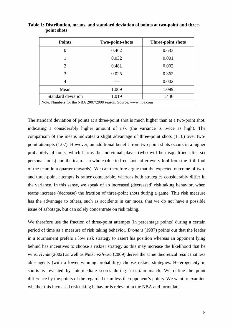
Table 1: Distribution, means, and standard deviation of points at two-point and three-point shots
Points Two-point-shots Three-point shots
0 0.462 0.633
1 0.032 0.001
2 0.481 0.002
3 0.025 0.362
4 --- 0.002
Mean 1.069 1.099 Standard deviation 1.019 1.446
Note: Numbers for the NBA 2007/2008 season. Source: www.nba.com
The standard deviation of points at a three-point shot is much higher than at a two-point shot,
indicating a considerably higher amount of risk (the variance is twice as high). The
comparison of the means indicates a slight advantage of three-point shots (1.10) over two-
point attempts (1.07). However, an additional benefit from two point shots occurs in a higher
probability of fouls, which harms the individual player (who will be disqualified after six
personal fouls) and the team as a whole (due to free shots after every foul from the fifth foul
of the team in a quarter onwards). We can therefore argue that the expected outcome of two-
and three-point attempts is rather comparable, whereas both strategies considerably differ in
the variance. In this sense, we speak of an increased (decreased) risk taking behavior, when
teams increase (decrease) the fraction of three-point shots during a game. This risk measure
has the advantage to others, such as accidents in car races, that we do not have a possible
issue of sabotage, but can solely concentrate on risk taking.
We therefore use the fraction of three-point attempts (in percentage points) during a certain
period of time as a measure of risk taking behavior. Bronars (1987) points out that the leader
in a tournament prefers a low risk strategy to assert his position whereas an opponent lying
behind has incentives to choose a riskier strategy as this may increase the likelihood that he
wins. Hvide (2002) as well as Nieken/Sliwka (2009) derive the same theoretical result that less
able agents (with a lower winning probability) choose riskier strategies. Heterogeneity in
sports is revealed by intermediate scores during a certain match. We define the point
difference by the points of the regarded team less the opponent’s points. We want to examine
whether this increased risk taking behavior is relevant in the NBA and formulate
6
Hypothesis 1:
The risk taking strategy of a team decreases in the point difference during a basketball
game in terms of the fraction of three-point shots.
Increasing the risk changes the random distribution of results in the way that probability mass
is shifted from the mean to the tails. Hence, extreme results become more likely. Since the
higher likelihood of a poor value is not harmful, because damage is limited to losing the
game, the increasing probability for a high result makes it more likely for the trailing team to
win the game after all. This consideration leads to
Hypothesis 2:
A change to a riskier strategy is beneficial for a team lying behind in terms of an
increased chance to win a game.
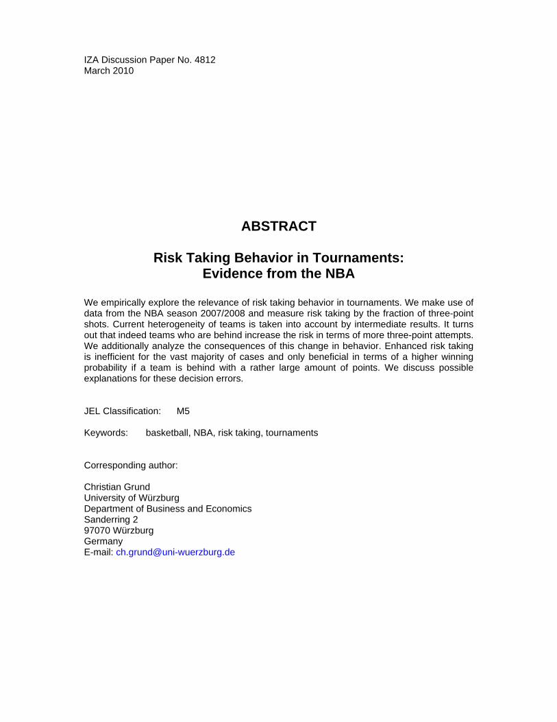
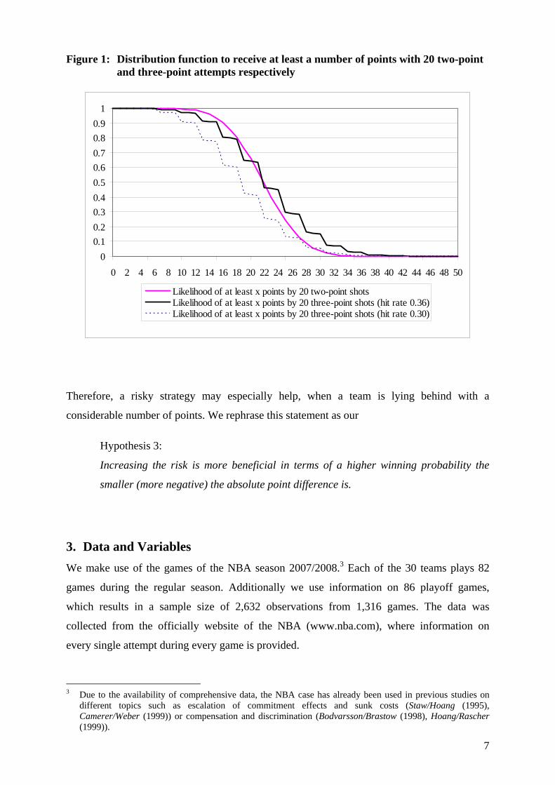
However, we have to consider that the hit rate for thee-point-shots may be influenced by the
risk strategy. Increasing the fraction of three-point shots may implicate attempts in situations,
in which is not appropriate to do so. A declining hit rate shifts the distribution function to the
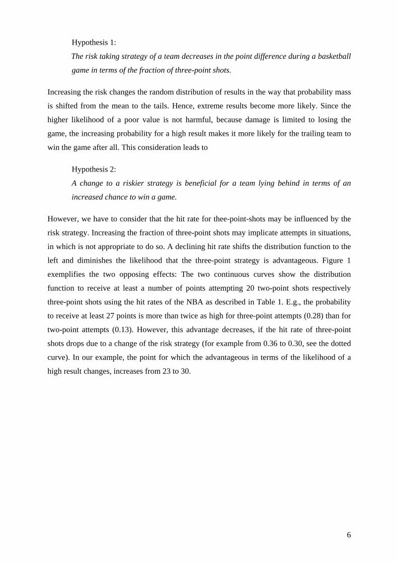
left and diminishes the likelihood that the three-point strategy is advantageous. Figure 1
exemplifies the two opposing effects: The two continuous curves show the distribution
function to receive at least a number of points attempting 20 two-point shots respectively
three-point shots using the hit rates of the NBA as described in Table 1. E.g., the probability
to receive at least 27 points is more than twice as high for three-point attempts (0.28) than for
two-point attempts (0.13). However, this advantage decreases, if the hit rate of three-point
shots drops due to a change of the risk strategy (for example from 0.36 to 0.30, see the dotted
curve). In our example, the point for which the advantageous in terms of the likelihood of a
high result changes, increases from 23 to 30.
7
Figure 1: Distribution function to receive at least a number of points with 20 two-point and three-point attempts respectively
00.10.20.30.40.50.60.70.80.9
1
0 2 4 6 8 10 12 14 16 18 20 22 24 26 28 30 32 34 36 38 40 42 44 46 48 50
Likelihood of at least x points by 20 two-point shotsLikelihood of at least x points by 20 three-point shots (hit rate 0.36)Likelihood of at least x points by 20 three-point shots (hit rate 0.30)
Therefore, a risky strategy may especially help, when a team is lying behind with a
considerable number of points. We rephrase this statement as our
Hypothesis 3:
Increasing the risk is more beneficial in terms of a higher winning probability the
smaller (more negative) the absolute point difference is.
3. Data and Variables We make use of the games of the NBA season 2007/2008.3 Each of the 30 teams plays 82
games during the regular season. Additionally we use information on 86 playoff games,
which results in a sample size of 2,632 observations from 1,316 games. The data was
collected from the officially website of the NBA (www.nba.com), where information on
every single attempt during every game is provided.
3 Due to the availability of comprehensive data, the NBA case has already been used in previous studies on
different topics such as escalation of commitment effects and sunk costs (Staw/Hoang (1995), Camerer/Weber (1999)) or compensation and discrimination (Bodvarsson/Brastow (1998), Hoang/Rascher (1999)).
8
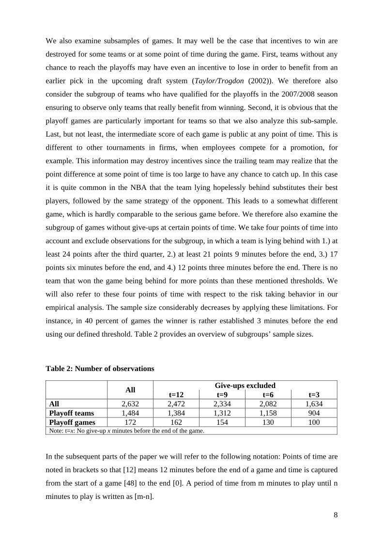
We also examine subsamples of games. It may well be the case that incentives to win are
destroyed for some teams or at some point of time during the game. First, teams without any
chance to reach the playoffs may have even an incentive to lose in order to benefit from an
earlier pick in the upcoming draft system (Taylor/Trogdon (2002)). We therefore also
consider the subgroup of teams who have qualified for the playoffs in the 2007/2008 season
ensuring to observe only teams that really benefit from winning. Second, it is obvious that the
playoff games are particularly important for teams so that we also analyze this sub-sample.
Last, but not least, the intermediate score of each game is public at any point of time. This is
different to other tournaments in firms, when employees compete for a promotion, for
example. This information may destroy incentives since the trailing team may realize that the
point difference at some point of time is too large to have any chance to catch up. In this case
it is quite common in the NBA that the team lying hopelessly behind substitutes their best
players, followed by the same strategy of the opponent. This leads to a somewhat different
game, which is hardly comparable to the serious game before. We therefore also examine the
subgroup of games without give-ups at certain points of time. We take four points of time into
account and exclude observations for the subgroup, in which a team is lying behind with 1.) at
least 24 points after the third quarter, 2.) at least 21 points 9 minutes before the end, 3.) 17
points six minutes before the end, and 4.) 12 points three minutes before the end. There is no
team that won the game being behind for more points than these mentioned thresholds. We
will also refer to these four points of time with respect to the risk taking behavior in our
empirical analysis. The sample size considerably decreases by applying these limitations. For
instance, in 40 percent of games the winner is rather established 3 minutes before the end
using our defined threshold. Table 2 provides an overview of subgroups’ sample sizes.
Table 2: Number of observations
Give-ups excluded All t=12 t=9 t=6 t=3 All 2,632 2,472 2,334 2,082 1,634 Playoff teams 1,484 1,384 1,312 1,158 904 Playoff games 172 162 154 130 100 Note: t=x: No give-up x minutes before the end of the game.
In the subsequent parts of the paper we will refer to the following notation: Points of time are
noted in brackets so that [12] means 12 minutes before the end of a game and time is captured
from the start of a game [48] to the end [0]. A period of time from m minutes to play until n
minutes to play is written as [m-n].
9
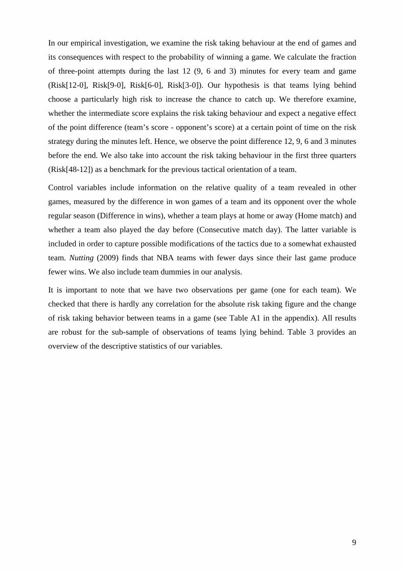
In our empirical investigation, we examine the risk taking behaviour at the end of games and
its consequences with respect to the probability of winning a game. We calculate the fraction
of three-point attempts during the last 12 (9, 6 and 3) minutes for every team and game
(Risk[12-0], Risk[9-0], Risk[6-0], Risk[3-0]). Our hypothesis is that teams lying behind
choose a particularly high risk to increase the chance to catch up. We therefore examine,
whether the intermediate score explains the risk taking behaviour and expect a negative effect
of the point difference (team’s score - opponent’s score) at a certain point of time on the risk
strategy during the minutes left. Hence, we observe the point difference 12, 9, 6 and 3 minutes
before the end. We also take into account the risk taking behaviour in the first three quarters
(Risk[48-12]) as a benchmark for the previous tactical orientation of a team.
Control variables include information on the relative quality of a team revealed in other
games, measured by the difference in won games of a team and its opponent over the whole
regular season (Difference in wins), whether a team plays at home or away (Home match) and
whether a team also played the day before (Consecutive match day). The latter variable is
included in order to capture possible modifications of the tactics due to a somewhat exhausted
team. Nutting (2009) finds that NBA teams with fewer days since their last game produce
fewer wins. We also include team dummies in our analysis.
It is important to note that we have two observations per game (one for each team). We
checked that there is hardly any correlation for the absolute risk taking figure and the change
of risk taking behavior between teams in a game (see Table A1 in the appendix). All results
are robust for the sub-sample of observations of teams lying behind. Table 3 provides an
overview of the descriptive statistics of our variables.
10
Table 3: Descriptive statistics (whole sample)
N Mean Sd Min Max Risk [48-12] 2632 20.83 7.585 1.587 49.09 Risk [12-0] 2632 26.11 12.36 0 70.00 Risk [9-0] 2632 26.89 13.72 0 80.00 Risk [6-0] 2632 27.94 16.92 0 87.50 Risk [3-0] 2631a 29.85 23.33 0 100.0 Point difference [12] 2632 0 12.81 -45 45 Point difference [9] 2632 0 13.24 -47 47 Point difference [6] 2632 0 13.64 -48 48 Point difference [3] 2632 0 14.15 -49 49 Home match 2632 0.500 0.500 0 1 Consecutive match day 2632 0.220 0.414 0 1 Difference in wins 2632 0.000 19.20 -51 51 a There is one team that did not shoot at all in the last three minutes of one game, so the risk figure can
not be determined.
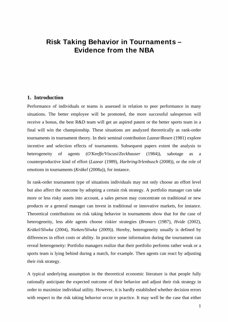
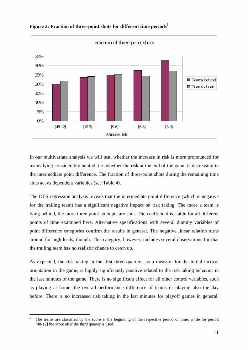
4. Results As a first result it can be established that both teams increase risk during the fourth quarter.
Figure 2 illustrates that teams behind go for more three-point attempts, especially in the last
three minutes, while the leading teams increase the risk only slightly. This result is even more
apparent, if give-ups are excluded (see Figure A1 in the appendix). The risk increase of the
teams being behind is in line with our first hypothesis. However, also the teams being ahead
before the last quarter increase the fraction of three-point shots significantly in the last 12
minutes of the game (t-test on two dependent samples; p=0.000 for both teams behind and
ahead).4
4 One may speculate that in some situations it is demanding for teams to push the ball near the basket. In this
case effort costs may rather increase for two-point attempts when players are exhausted at the end of the game. Therefore, a general increase in three-point shots may occur.
11
Figure 2: Fraction of three-point shots for different time periods5
Fraction of three-point shots
0%
5%
10%
15%
20%
25%
30%
35%
[48-12] [12-9] [9-6] [6-3] [3-0]
Minutes left
Teams behindTeams ahead
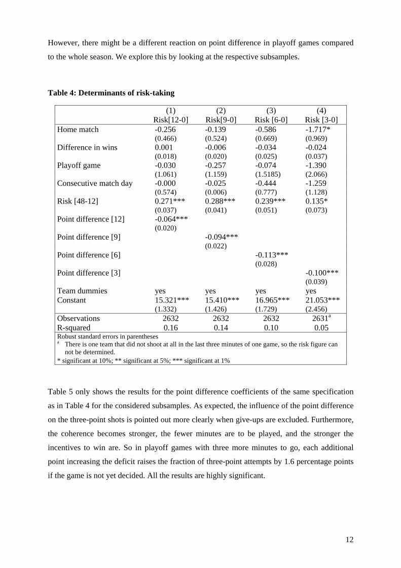
In our multivariate analysis we will test, whether the increase in risk is more pronounced for
teams lying considerably behind, i.e. whether the risk at the end of the game is decreasing in
the intermediate point difference. The fraction of three-point shots during the remaining time
slots act as dependent variables (see Table 4).
The OLS regression analysis reveals that the intermediate point difference (which is negative
for the trailing team) has a significant negative impact on risk taking. The more a team is
lying behind, the more three-point attempts are shot. The coefficient is stable for all different
points of time examined here. Alternative specifications with several dummy variables of
point difference categories confirm the results in general. The negative linear relation turns
around for high leads, though. This category, however, includes several observations for that
the trailing team has no realistic chance to catch up.
As expected, the risk taking in the first three quarters, as a measure for the initial tactical
orientation in the game, is highly significantly positive related to the risk taking behavior in
the last minutes of the game. There is no significant effect for all other control variables, such
as playing at home, the overall performance difference of teams or playing also the day
before. There is no increased risk taking in the last minutes for playoff games in general.
5 The teams are classified by the score at the beginning of the respective period of time, while for period
[48-12] the score after the third quarter is used.
12
However, there might be a different reaction on point difference in playoff games compared
to the whole season. We explore this by looking at the respective subsamples.
Table 4: Determinants of risk-taking
(1) (2) (3) (4) Risk[12-0] Risk[9-0] Risk [6-0] Risk [3-0] Home match -0.256 -0.139 -0.586 -1.717* (0.466) (0.524) (0.669) (0.969) Difference in wins 0.001 -0.006 -0.034 -0.024 (0.018) (0.020) (0.025) (0.037) Playoff game -0.030 -0.257 -0.074 -1.390 (1.061) (1.159) (1.5185) (2.066) Consecutive match day -0.000 -0.025 -0.444 -1.259 (0.574) (0.006) (0.777) (1.128) Risk [48-12] 0.271*** 0.288*** 0.239*** 0.135* (0.037) (0.041) (0.051) (0.073) Point difference [12] -0.064*** (0.020) Point difference [9] -0.094*** (0.022) Point difference [6] -0.113*** (0.028) Point difference [3] -0.100*** (0.039) Team dummies yes yes yes yes Constant 15.321*** 15.410*** 16.965*** 21.053*** (1.332) (1.426) (1.729) (2.456) Observations 2632 2632 2632 2631a
R-squared 0.16 0.14 0.10 0.05 Robust standard errors in parentheses a There is one team that did not shoot at all in the last three minutes of one game, so the risk figure can
not be determined. * significant at 10%; ** significant at 5%; *** significant at 1%
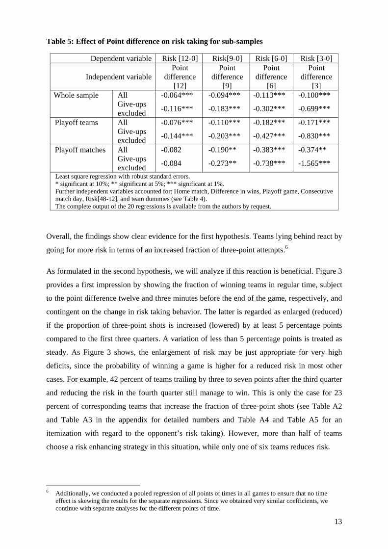
Table 5 only shows the results for the point difference coefficients of the same specification
as in Table 4 for the considered subsamples. As expected, the influence of the point difference
on the three-point shots is pointed out more clearly when give-ups are excluded. Furthermore,
the coherence becomes stronger, the fewer minutes are to be played, and the stronger the
incentives to win are. So in playoff games with three more minutes to go, each additional
point increasing the deficit raises the fraction of three-point attempts by 1.6 percentage points
if the game is not yet decided. All the results are highly significant.
13
Table 5: Effect of Point difference on risk taking for sub-samples
Dependent variable Risk [12-0] Risk[9-0] Risk [6-0] Risk [3-0]
Independent variable Point
difference [12]
Point difference
[9]
Point difference
[6]
Point difference
[3] Whole sample All -0.064*** -0.094*** -0.113*** -0.100*** Give-ups
excluded -0.116*** -0.183*** -0.302*** -0.699***
Playoff teams All -0.076*** -0.110*** -0.182*** -0.171*** Give-ups
excluded -0.144*** -0.203*** -0.427*** -0.830***
Playoff matches All -0.082 -0.190** -0.383*** -0.374** Give-ups
excluded -0.084 -0.273** -0.738*** -1.565*** Least square regression with robust standard errors. * significant at 10%; ** significant at 5%; *** significant at 1%. Further independent variables accounted for: Home match, Difference in wins, Playoff game, Consecutive match day, Risk[48-12], and team dummies (see Table 4). The complete output of the 20 regressions is available from the authors by request.
Overall, the findings show clear evidence for the first hypothesis. Teams lying behind react by
going for more risk in terms of an increased fraction of three-point attempts.6
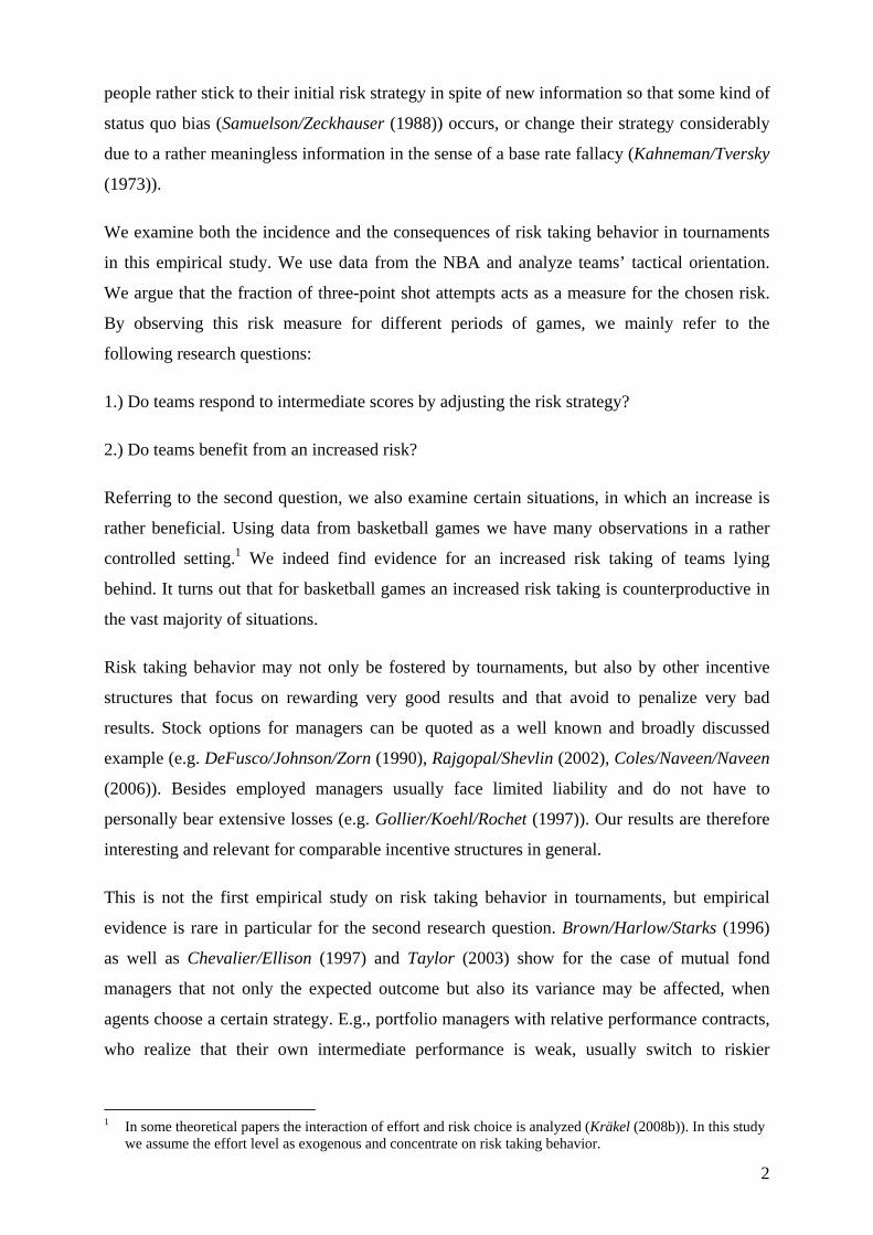
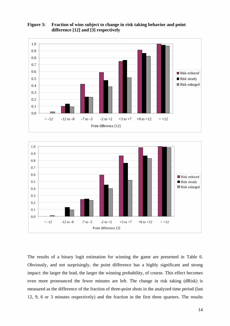
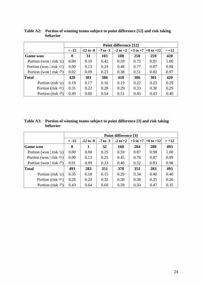
As formulated in the second hypothesis, we will analyze if this reaction is beneficial. Figure 3
provides a first impression by showing the fraction of winning teams in regular time, subject
to the point difference twelve and three minutes before the end of the game, respectively, and
contingent on the change in risk taking behavior. The latter is regarded as enlarged (reduced)
if the proportion of three-point shots is increased (lowered) by at least 5 percentage points
compared to the first three quarters. A variation of less than 5 percentage points is treated as
steady. As Figure 3 shows, the enlargement of risk may be just appropriate for very high
deficits, since the probability of winning a game is higher for a reduced risk in most other
cases. For example, 42 percent of teams trailing by three to seven points after the third quarter
and reducing the risk in the fourth quarter still manage to win. This is only the case for 23
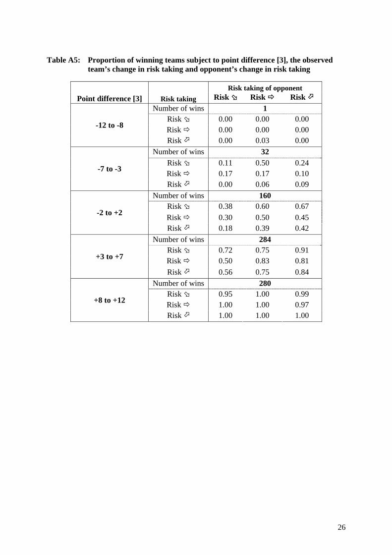
percent of corresponding teams that increase the fraction of three-point shots (see Table A2
and Table A3 in the appendix for detailed numbers and Table A4 and Table A5 for an
itemization with regard to the opponent’s risk taking). However, more than half of teams
choose a risk enhancing strategy in this situation, while only one of six teams reduces risk.
6 Additionally, we conducted a pooled regression of all points of times in all games to ensure that no time
effect is skewing the results for the separate regressions. Since we obtained very similar coefficients, we continue with separate analyses for the different points of time.
14
Figure 3: Fraction of wins subject to change in risk taking behavior and point difference [12] and [3] respectively
0.0
0.1
0.2
0.3
0.4
0.5
0.6
0.7
0.8
0.9
1.0
< -12 -12 to -8 -7 to -3 -2 to +2 +3 to +7 +8 to +12 > +12
Point difference [12]
Risk reducedRisk steadyRisk enlarged
0.0
0.1
0.2
0.3
0.4
0.5
0.6
0.7
0.8
0.9
1.0
< -12 -12 to -8 -7 to -3 -2 to +2 +3 to +7 +8 to +12 > +12
Point difference [3]
Risk reducedRisk steadyRisk enlarged
The results of a binary logit estimation for winning the game are presented in Table 6.
Obviously, and not surprisingly, the point difference has a highly significant and strong
impact: the larger the lead, the larger the winning probability, of course. This effect becomes
even more pronounced the fewer minutes are left. The change in risk taking (dRisk) is
measured as the difference of the fraction of three-point shots in the analyzed time period (last
12, 9, 6 or 3 minutes respectively) and the fraction in the first three quarters. The results
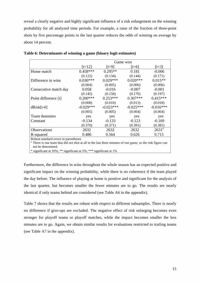
15
reveal a clearly negative and highly significant influence of a risk enlargement on the winning
probability for all analyzed time periods. For example, a raise of the fraction of three-point
shots by five percentage points in the last quarter reduces the odds of winning on average by
about 14 percent.
Table 6: Determinants of winning a game (binary logit estimates)
Game won [t=12] [t=9] [t=6] [t=3] Home match 0.458*** 0.295** 0.181 -0.006 (0.122) (0.134) (0.144) (0.171) Difference in wins 0.030*** 0.029*** 0.020*** 0.015** (0.004) (0.005) (0.006) (0.006) Consecutive match day 0.058 -0.016 -0.007 -0.001 (0.145) (0.158) (0.170) (0.197) Point difference [t] 0.200*** 0.253*** 0.307*** 0.415*** (0.008) (0.010) (0.013) (0.018) dRisk[t-0] -0.029*** -0.023*** -0.025*** -0.016*** (0.005) (0.005) (0.004) (0.004) Team dummies yes yes yes yes Constant -0.134 -0.133 -0.123 -0.169 (0.370) (0.371) (0.391) (0.381) Observations 2632 2632 2632 2631a
R-squared 0.486 0.564 0.626 0.715 Robust standard errors in parentheses a There is one team that did not shot at all in the last three minutes of one game, so the risk figure can
not be determined. * significant at 10%; ** significant at 5%; *** significant at 1%
Furthermore, the difference in wins throughout the whole season has an expected positive and
significant impact on the winning probability, while there is no coherence if the team played
the day before. The influence of playing at home is positive and significant for the analysis of
the last quarter, but becomes smaller the fewer minutes are to go. The results are nearly
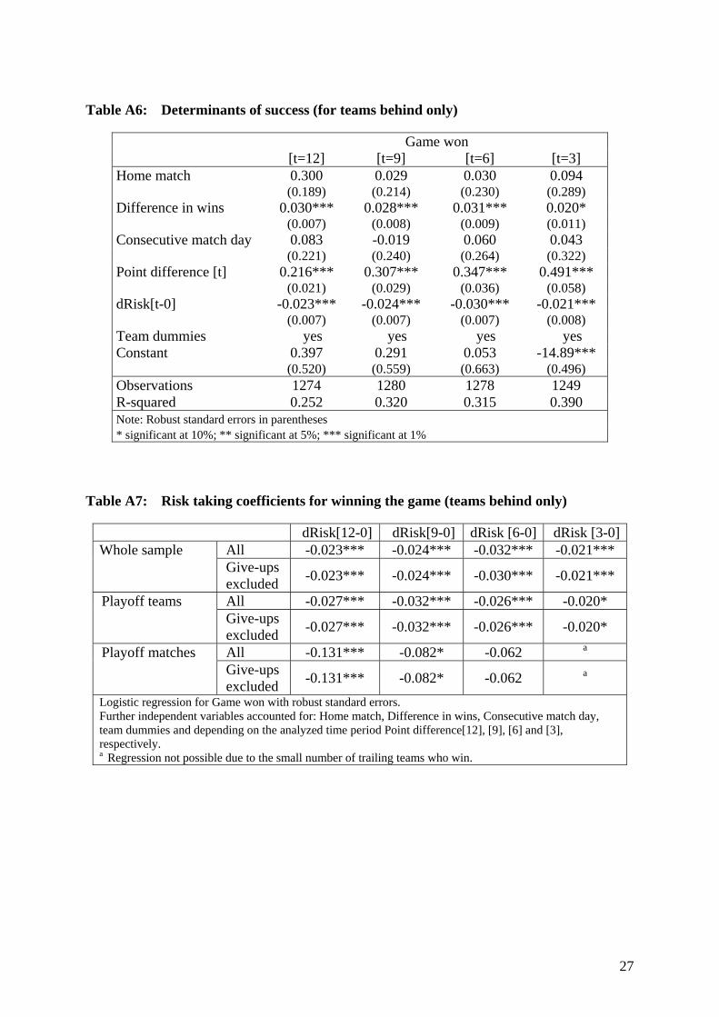
identical if only teams behind are considered (see Table A6 in the appendix).
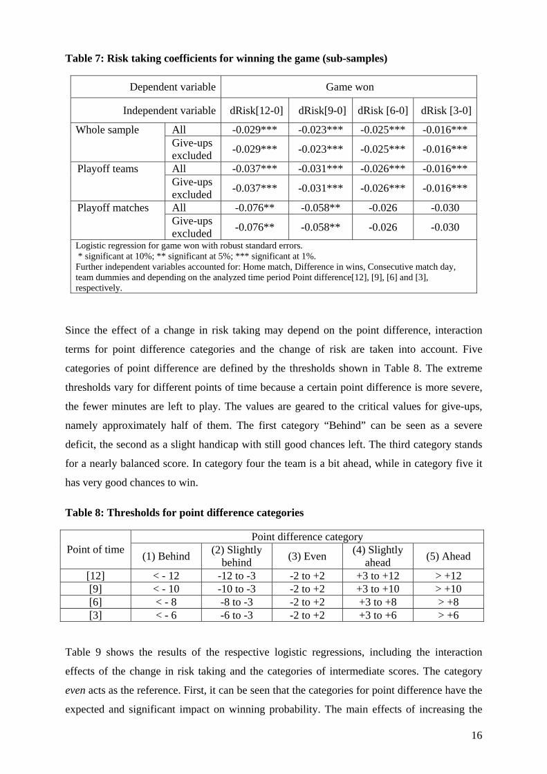
Table 7 shows that the results are robust with respect to different subsamples. There is nearly
no difference if give-ups are excluded. The negative effect of risk enlarging becomes even
stronger for playoff teams or playoff matches, while the impact becomes smaller the less
minutes are to go. Again, we obtain similar results for evaluations restricted to trailing teams
(see Table A7 in the appendix).
16
Table 7: Risk taking coefficients for winning the game (sub-samples)
Dependent variable Game won
Independent variable dRisk[12-0] dRisk[9-0] dRisk [6-0] dRisk [3-0]
Whole sample All -0.029*** -0.023*** -0.025*** -0.016*** Give-ups
excluded -0.029*** -0.023*** -0.025*** -0.016***
Playoff teams All -0.037*** -0.031*** -0.026*** -0.016*** Give-ups
excluded -0.037*** -0.031*** -0.026*** -0.016***
Playoff matches All -0.076** -0.058** -0.026 -0.030 Give-ups
excluded -0.076** -0.058** -0.026 -0.030 Logistic regression for game won with robust standard errors. * significant at 10%; ** significant at 5%; *** significant at 1%.
Further independent variables accounted for: Home match, Difference in wins, Consecutive match day, team dummies and depending on the analyzed time period Point difference[12], [9], [6] and [3], respectively.
Since the effect of a change in risk taking may depend on the point difference, interaction
terms for point difference categories and the change of risk are taken into account. Five
categories of point difference are defined by the thresholds shown in Table 8. The extreme
thresholds vary for different points of time because a certain point difference is more severe,
the fewer minutes are left to play. The values are geared to the critical values for give-ups,
namely approximately half of them. The first category “Behind” can be seen as a severe
deficit, the second as a slight handicap with still good chances left. The third category stands
for a nearly balanced score. In category four the team is a bit ahead, while in category five it
has very good chances to win.
Table 8: Thresholds for point difference categories
Point difference category Point of time (1) Behind (2) Slightly
behind (3) Even (4) Slightly ahead (5) Ahead
[12] < - 12 -12 to -3 -2 to +2 +3 to +12 > +12 [9] < - 10 -10 to -3 -2 to +2 +3 to +10 > +10 [6] < - 8 -8 to -3 -2 to +2 +3 to +8 > +8 [3] < - 6 -6 to -3 -2 to +2 +3 to +6 > +6
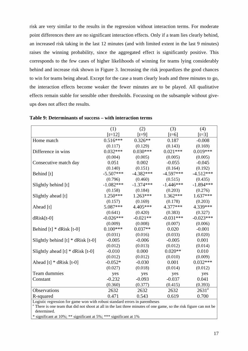
Table 9 shows the results of the respective logistic regressions, including the interaction
effects of the change in risk taking and the categories of intermediate scores. The category
even acts as the reference. First, it can be seen that the categories for point difference have the
expected and significant impact on winning probability. The main effects of increasing the
17
risk are very similar to the results in the regression without interaction terms. For moderate
point differences there are no significant interaction effects. Only if a team lies clearly behind,
an increased risk taking in the last 12 minutes (and with limited extent in the last 9 minutes)
raises the winning probability, since the aggregated effect is significantly positive. This
corresponds to the few cases of higher likelihoods of winning for teams lying considerably
behind and increase risk shown in Figure 3. Increasing the risk jeopardizes the good chances
to win for teams being ahead. Except for the case a team clearly leads and three minutes to go,
the interaction effects become weaker the fewer minutes are to be played. All qualitative
effects remain stable for sensible other thresholds. Focussing on the subsample without give-
ups does not affect the results.
Table 9: Determinants of success – with interaction terms
(1) (2) (3) (4) [t=12] [t=9] [t=6] [t=3] Home match 0.516*** 0.326** 0.187 -0.008 (0.117) (0.129) (0.143) (0.169) Difference in wins 0.032*** 0.030*** 0.021*** 0.019*** (0.004) (0.005) (0.005) (0.005) Consecutive match day 0.051 0.002 -0.055 -0.045 (0.140) (0.151) (0.164) (0.192) Behind [t] -5.507*** -4.382*** -4.597*** -4.512*** (0.796) (0.460) (0.515) (0.435) Slightly behind [t] -1.082*** -1.374*** -1.446*** -1.894*** (0.158) (0.184) (0.203) (0.276) Slightly ahead [t] 1.250*** 1.263*** 1.362*** 1.637*** (0.157) (0.169) (0.178) (0.203) Ahead [t] 5.087*** 4.405*** 4.377*** 4.339*** (0.641) (0.420) (0.383) (0.327) dRisk[t-0] -0.026*** -0.021** -0.031*** -0.023*** (0.009) (0.008) (0.007) (0.006) Behind [t] * dRisk [t-0] 0.100*** 0.037** 0.020 -0.001 (0.031) (0.016) (0.033) (0.020) Slightly behind [t] * dRisk [t-0] -0.005 -0.006 -0.005 0.001 (0.012) (0.013) (0.012) (0.014) Slightly ahead [t] * dRisk [t-0] -0.010 0.000 0.020** 0.010 (0.012) (0.012) (0.010) (0.009) Ahead [t] * dRisk [t-0] -0.052* -0.030 0.001 0.032***
(0.027) (0.018) (0.014) (0.012) Team dummies yes yes yes yes Constant -0.232 -0.093 -0.037 0.041 (0.360) (0.377) (0.415) (0.393) Observations 2632 2632 2632 2631a
R-squared 0.471 0.543 0.619 0.700 Logistic regression for game won with robust standard errors in parentheses a There is one team that did not shoot at all in the last three minutes of one game, so the risk figure can not be
determined. * significant at 10%; ** significant at 5%; *** significant at 1%
18
To sum up, our results show that risk enlarging is not beneficial in most cases. So
hypothesis 2 has to be rejected. Hypothesis 3 is supported in the regressions for 12 and 9
minutes to go in terms of a positive interaction effect between point difference categories and
changes in risk taking.
This rises the question why teams react by enlarging the risk, although this strategy is usually
not appropriate. A possible explanation may be that the teams systematically overestimate the
benefit of increasing the fraction of three-point shots in the sense of the base-rate fallacy.
They may give too much weight to the new information (point difference) and too little to the
basic information that resulted in the originally chosen risk strategy. It may well be the case
that some public pressure from spectators, or the owner of the clubs, leads to a change in risk
strategy. If a deficit becomes obvious, retaining the strategy might be interpreted as ignoring
the situation and not trying everything to catch up in the remaining time. Anticipating this,
coaches may even take more risk in order to signal a kind of pro-active behavior when being
aware of a decreasing winning probability.
5. Conclusion The strategy of individuals or teams with respect to risk taking is highly relevant in many
tournament kind of situations, when subjects are assessed in relation to each other. Making
use of basketball data, we show that protagonists indeed adjust their risk strategy based on
new information concerning the intermediate score in a game. Trailing teams increase the
fraction of three-point shots in the last minutes of a game. Surprisingly, this reaction is not
beneficial in terms of an increasing winning probability in most cases.
Therefore, teams lying behind take too much risk too early in a game. This decision error may
firstly be interpreted as irrational behavior of the coaches in charge of the strategy. Coaches
may underestimate decreasing hit rates at increased risks. This may partly be explained by
choking under pressure, which is defined as performance decrements under circumstances
that increase the importance of good or improved performance (Baumeister (1984)). Players
may become aware of the importance of an improved performance especially when coaches
announce changes in strategy. Baumeister/Steinhilber (1984) show for several cases that this
pressure can be relevant for the home teams in particular. However, we do not find
indications in our data that home teams increase risks to a greater extent or that they are
particularly affected by the following failures. Second, the hasty increased risk taking may be
interpreted as a reaction to some incentives of signalling pro-active behavior due to public
19
pressure as mentioned above.7 If this second argument is relevant, this is contrary to career
concerns or herding behavior of managers, who have incentives to stick to their initial
strategy and abstain from innovative, not well established, investment decisions due to certain
incentives (see Kanodia/Bushman/Dickhaut (1989), Scharfstein/Stein (1990)).
Whether individuals take risks rather cautiously or distinctively, obviously depends on
incentives for achieving very good or avoiding very bad results. A team lying behind in a
basketball game only benefits from a very good result in the remaining time that is sufficient
for catching up and winning the game. Stock option plans or limited liability of managers
induce similar effects. In contrast, managers may rather want to ensure their own jobs by
avoiding very bad results. This is in line with experimental evidence by Gaba/Kalra (1999),
who find that risk taking behavior in tournaments is decreasing in the number of winners for a
given number of participants.
The three-point rule has been introduced by the NBA in the season 1979/1980 to make the
game more interesting, and indeed we find that for the case of a team lying considerably
behind the three-point shot strategy is an appropriate tool to catch up, although this strategy is
used too early in many cases. Implementing an appropriate incentive system for risk taking is
a huge challenge for a principal, and the systems are supposed to differ considerably between
portfolio managers and R&D teams, for instance. Based on our results, club owners (who are
aware of the decision errors) may adopt incentives for coaches and/or players by introducing a
fine for defeats with many points, for instance.8
A possible correlation of the outcomes of risky strategy across opponents has to be taken into
account for a number of cases. Nieken/Sliwka (2009) show theoretically and experimentally
that for the case of a high correlation, it may be beneficial for a leading agent to simulate the
opponent’s (risky) strategy. This effect is likely to be relevant for portfolio managers, for
instance. However, a considerable correlation of the result of three-point shots is not likely in
basketball games.
Future research may compare risk taking behavior and its consequences in different incentive
structures systematically.
7 If this is true, the effect is similar to the phenomenon that coaches in professional team sports are dismissed
quite often (due to public pressure), even though the benefits of such a proceeding are not evidenced (see Wirl/Sagmeister (2008)).
8 Gilpatric (2009) shows theoretically that some sanctions for worst performance can inhibit pronounced risk taking.
20
References Baumeister, Roy F. (1984): Choking Under Pressure: Self-Consciousness and Paradoxical
Effects of Incentives on Skillful Performance, in: Journal of Personality and Social Psychology 46, 610-620.
Baumeister, Roy F./Steinhilber, Andrew (1984): Paradoxical Effects of Supportive Audiences
on Performance Under Pressure: The Home Field Disadvantage in Sports Championships, in: Journal of Personality and Social Psychology 47, 85-93.
Becker, Brian E./Huselid, Mark A. (1992): The Incentive Effects of Tournament
Compensation Systems, in: Administrative Science Quarterly 37, 336-350. Bodvarsson, Örn B./Brastow, Raymond T. (1998): Do Employers Pay for Consistent
Performance: Evidence from the NBA, in: Economic Inquiry 36, 145-160. Bothner, Matthew S./Kang, Jeong-han/Stuart, Toby E. (2007): Competitive Crowding and
Risk Taking in a Tournament: Evidence from NASCAR Racing, in: Administrative Science Quarterly 52, 208-247.
Bronars, Stephen (1987): Risk Taking in Tournaments, Working Paper, University of Texas,
Austin. Brown, Keith C./Harlow, W. V./Starks, Laura T. (1996): Of Tournaments and Temptations:
An Analysis of Managerial Incentives in the Mutual Fund Industry, in: The Journal of Finance 51, 85-110.
Camerer, Colin F./Weber, Roberto A. (1999): The Econometrics and Behavioral Economics
of Escalation of Commitment: A Re-examination of Staw and Hoang's NBA Data, in: Journal of Economic Behavior & Organization 39, 59-82.
Chevalier, Judith A./Ellison, Glenn D. (1997): Risk Taking by Mutual Funds as a Response to
Incentives, in: Journal of Political Economy 105, 1167-1200. Coles, Jeffrey L./Naveen, Daniel D./Naveen, Lalitha (2006): Managerial Incentives and Risk
Taking, in: Journal of Financial Economics 79, 431-468. DeFusco, Richard A./Johnson, Robert R./Zorn, Thomas S. (1990): The Effect of Executive
Stock Option Plans on Stockholders and Bondholders, in: Journal of Finance 45, 617-627.
Gaba, Anil/Kalra, Ajay (1999): Risk Behavior in Response to Quotas and Contests, in:
Marketing Science 18, 417-434. Garicano, Luis/Palacios-Huerta, Ignacio (2005): Sabotage in Tournaments: Making the
Beautiful Game a Bit Less Beautiful, CRPR Discussion Paper No. 5231. Genakos, Christos/Pagliero, Mario (2009): Risk Taking and Performance in Multistage
Tournaments: Evidence from Weightlifting Competitions, in: CEP Discussion Paper No. 928 London,
21
Gilpatric, Scott M. (2009): Risk taking in contests and the role of carrots and sticks, in: Economic Inquiry 47, 266-277.
Gollier, Christian/Koehl, Pierre-Francois/Rochet, Jean-Charles (1997): Risk-taking
Behavior with Limited Liability and Risk Aversion, in: Journal of Risk and Insurance 64, 347-370.
Grund, Christian/Gürtler, Oliver (2005): An empirical study on risk-taking in tournaments,
in: Applied Economics Letters 12, 457-461. Harbring, Christiane/Irlenbusch, Bernd (2008): How Many Winners are Good to Have? On
Tournaments with Sabotage, in: Journal of Economic Behavior & Organization 65, 682-702.
Hoang, Ha/Rascher, Dan (1999): The NBA, Exit Discrimination, and Career Earnings, in:
Industrial Relations 38, 69-91. Hvide, Hans K. (2002): Tournament Rewards and Risk Taking, in: Journal of Labor
Economics 20, 877-898. Kahneman, Daniel/Tversky, Amos (1973): On the psychology of prediction, in: Psychological
review 80, 237-257. Kanodia, Chandra/Bushman, Robert/Dickhaut, John (1989): Escalation Errors and the Sunk
Cost Effect: An Explanation Based on Reputation and Information Asymmetries, in: Journal of Accounting Research 27, 59-77.
Kempf, Alexander/Ruenzi, Stefan/Thiele, Tanja (2009): Employment risk, compensation
incentives, and managerial risk taking: Evidence from the mutual fund industry, in: Journal of Financial Economics 92, 92-108.
Kräkel, Matthias (2008a): Emotions in Tournaments, in: Journal of Economic Behavior &
Organization 67, 204-214. Kräkel, Matthias (2008b): Optimal risk taking in an uneven tournament game with risk averse
players, in: Journal of Mathematical Economics 44, 1219-1231. Kräkel, Matthias/Sliwka, Dirk (2004): Risk Taking in Asymmetric Tournaments, in: German
Economic Review 5, 103-116. Lazear, Edward P. (1989): Pay Equality and Industrial Politics, in: Journal of Political
Economy 97, 561-580. Lazear, Edward P./Rosen, Sherwin (1981): Rank-Order Tournaments as Optimum Labor
Contracts, in: Journal of Political Economy 89, 841-864. Lee, Jungmin (2004): Prize and Risk-Taking Strategy in Tournaments: Evidence from
Professional Poker Players, IZA Discussion Paper, No. 1345, Nieken, Petra/Sliwka, Dirk (2009): Risk-taking tournaments - Theory and experimental
evidence, in: Journal of Economic Psychology (in print), doi: 10.1016/j.joep.2009.03.009,
22
Nutting, Andrew W. (2009): Travel Costs in the NBA Production Function, in: Journal of
Sports Economics (in print), doi: 10.1177/1527002509355637 O'Keeffe, Mary/Viscusi, W. Kip/Zeckhauser, Richard J. (1984): Economic Contests:
Comparative Reward Schemes, in: Journal of Labor Economics 2, 27-56. Rajgopal, Shivaram/Shevlin, Terry (2002): Empirical Evidence on the Relation Between
Stock Option Compensation and Risk Taking, in: Journal of Accounting and Economics 33, 145-171.
Samuelson, William/Zeckhauser, Richard (1988): Status Quo Bias in Decision Making, in:
Journal of Risk and Uncertainty 1, 7-59. Scharfstein, David S./Stein, Jeremy C. (1990): Herd Behavior and Investment, in: American
Economic Review 80, 465-479. Staw, Berry M./Hoang, Ha (1995): Sunk costs in the NBA: Why Draft Order Affects Playing
Time and Survival in Professional Basketball, in: Administrative Science Quarterly 40, 474-494.
Taylor, Beck A./Trogdon, Justin G. (2002): Losing to Win: Tournament Incentives in the
National Basketball Association, in: Journal of Labor Economics 20, 23-41. Taylor, Jonathan (2003): Risk-taking behavior in mutual fund tournaments, in: Journal of
Economic Behavior & Organization 50, 373-383. Wirl, Franz/Sagmeister, Simon (2008): Changing of the Guards: New Coaches in Austria's
Premier Football League, in: Empirica 35, 267-278.
23
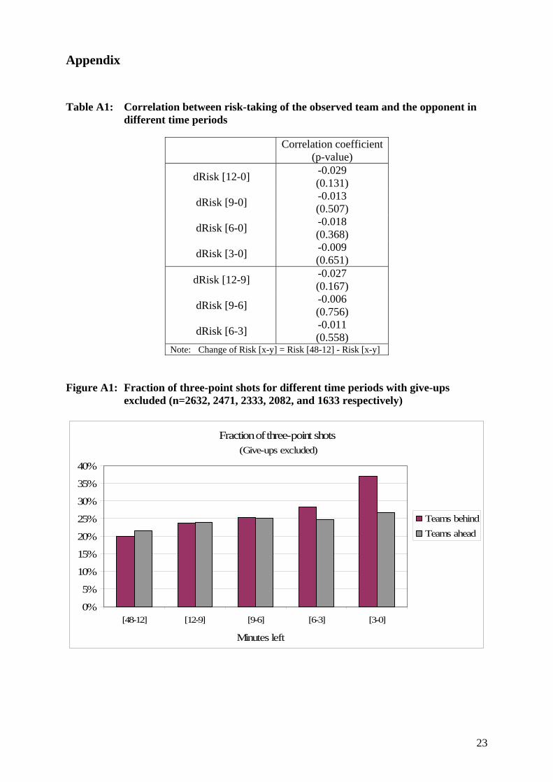
Appendix Table A1: Correlation between risk-taking of the observed team and the opponent in
different time periods
Correlation coefficient(p-value)
dRisk [12-0] -0.029 (0.131)
dRisk [9-0] -0.013 (0.507)
dRisk [6-0] -0.018 (0.368)
dRisk [3-0] -0.009 (0.651)
dRisk [12-9] -0.027 (0.167)
dRisk [9-6] -0.006 (0.756)
dRisk [6-3] -0.011 (0.558)
Note: Change of Risk [x-y] = Risk [48-12] - Risk [x-y] Figure A1: Fraction of three-point shots for different time periods with give-ups
excluded (n=2632, 2471, 2333, 2082, and 1633 respectively)
Fraction of three-point shots (Give-ups excluded)
0%
5%
10%
15%
20%
25%
30%
35%
40%
[48-12] [12-9] [9-6] [6-3] [3-0]
Minutes left
Teams behindTeams ahead
24
Table A2: Portion of winning teams subject to point difference [12] and risk taking
behavior
Point difference [12] < -12 -12 to -8 -7 to -3 -2 to +2 +3 to +7 +8 to +12 > +12
Game won 0 31 103 188 250 259 420 Portion (won | risk ) 0.00 0.10 0.42 0.59 0.75 0.91 1.00 Portion (won | risk ) 0.00 0.13 0.24 0.48 0.77 0.87 0.98 Portion (won | risk ) 0.02 0.09 0.23 0.38 0.51 0.82 0.97
Total 420 301 386 418 386 301 420 Portion (risk ) 0.19 0.17 0.16 0.19 0.22 0.23 0.29 Portion (risk ) 0.31 0.22 0.28 0.29 0.33 0.30 0.29 Portion (risk ) 0.49 0.60 0.54 0.51 0.45 0.43 0.40
Table A3: Portion of winning teams subject to point difference [3] and risk taking behavior
Point difference [3] < -12 -12 to -8 -7 to -3 -2 to +2 +3 to +7 +8 to +12 > +12
Game won 0 1 32 160 284 280 493 Portion (won | risk ) 0.00 0.00 0.25 0.59 0.87 0.98 1.00 Portion (won | risk ) 0.00 0.13 0.25 0.45 0.76 0.87 0.99 Portion (won | risk ) 0.01 0.09 0.23 0.40 0.52 0.83 0.98
Total 493 283 351 378 351 283 493 Portion (risk ) 0.35 0.18 0.15 0.29 0.34 0.40 0.40 Portion (risk ) 0.26 0.24 0.32 0.30 0.36 0.35 0.26 Portion (risk ) 0.43 0.64 0.60 0.59 0.50 0.47 0.35

25
Table A4: Proportion of winning teams subject to point difference [12], the observed
team’s change in risk taking and opponent’s change in risk taking
Risk taking of opponent Point difference [12] Risk taking Risk Risk Risk
Number of wins 31 Risk 0.00 0.00 0.25 Risk 0.00 0.13 0.18 -12 to -8
Risk 0.07 0.11 0.10 Number of wins 103
Risk 0.50 0.35 0.41 Risk 0.12 0.14 0.40 -7 to -3
Risk 0.11 0.19 0.32 Number of wins 188
Risk 0.44 0.52 0.68 Risk 0.43 0.43 0.47 -2 to +2
Risk 0.20 0.45 0.44 Number of wins 250
Risk 0.46 0.84 0.78 Risk 0.65 0.76 0.79 +3 to +7
Risk 0.52 0.50 0.53 Number of wins 259
Risk 0.91 0.92 0.91 Risk 0.89 0.87 0.86 +8 to +12
Risk 0.70 0.79 0.88
26
Table A5: Proportion of winning teams subject to point difference [3], the observed
team’s change in risk taking and opponent’s change in risk taking
Risk taking of opponent Point difference [3] Risk taking Risk Risk Risk
Number of wins 1 Risk 0.00 0.00 0.00 Risk 0.00 0.00 0.00 -12 to -8
Risk 0.00 0.03 0.00 Number of wins 32
Risk 0.11 0.50 0.24 Risk 0.17 0.17 0.10 -7 to -3
Risk 0.00 0.06 0.09 Number of wins 160
Risk 0.38 0.60 0.67 Risk 0.30 0.50 0.45 -2 to +2
Risk 0.18 0.39 0.42 Number of wins 284
Risk 0.72 0.75 0.91 Risk 0.50 0.83 0.81 +3 to +7
Risk 0.56 0.75 0.84 Number of wins 280
Risk 0.95 1.00 0.99 Risk 1.00 1.00 0.97 +8 to +12
Risk 1.00 1.00 1.00
27
Table A6: Determinants of success (for teams behind only)
Game won [t=12] [t=9] [t=6] [t=3] Home match 0.300 0.029 0.030 0.094 (0.189) (0.214) (0.230) (0.289) Difference in wins 0.030*** 0.028*** 0.031*** 0.020* (0.007) (0.008) (0.009) (0.011) Consecutive match day 0.083 -0.019 0.060 0.043 (0.221) (0.240) (0.264) (0.322) Point difference [t] 0.216*** 0.307*** 0.347*** 0.491*** (0.021) (0.029) (0.036) (0.058) dRisk[t-0] -0.023*** -0.024*** -0.030*** -0.021*** (0.007) (0.007) (0.007) (0.008) Team dummies yes yes yes yes Constant 0.397 0.291 0.053 -14.89*** (0.520) (0.559) (0.663) (0.496) Observations 1274 1280 1278 1249 R-squared 0.252 0.320 0.315 0.390 Note: Robust standard errors in parentheses * significant at 10%; ** significant at 5%; *** significant at 1%
Table A7: Risk taking coefficients for winning the game (teams behind only)
dRisk[12-0] dRisk[9-0] dRisk [6-0] dRisk [3-0]Whole sample All -0.023*** -0.024*** -0.032*** -0.021*** Give-ups
excluded -0.023*** -0.024*** -0.030*** -0.021***
Playoff teams All -0.027*** -0.032*** -0.026*** -0.020* Give-ups
excluded -0.027*** -0.032*** -0.026*** -0.020*
Playoff matches All -0.131*** -0.082* -0.062 a
Give-ups excluded -0.131*** -0.082* -0.062 a
Logistic regression for Game won with robust standard errors. Further independent variables accounted for: Home match, Difference in wins, Consecutive match day, team dummies and depending on the analyzed time period Point difference[12], [9], [6] and [3], respectively. a Regression not possible due to the small number of trailing teams who win.