NBER WORKING PAPER SERIES

RISK MATTERS: THE REAL EFFECTS OF VOLATILITY SHOCKS

Jesús Fernández-VillaverdePablo A. Guerrón-Quintana

Juan Rubio-RamírezMartín Uribe

Working Paper 14875http://www.nber.org/papers/w14875

NATIONAL BUREAU OF ECONOMIC RESEARCH1050 Massachusetts Avenue

Cambridge, MA 02138April 2009

We thank Marco Bomono, Javier García-Cicco, Alejandro Justiniano, Jim Hamilton, Kolver Hernandez,Ralph Koijen and participants at various seminars and conferences for useful comments. Beyond theusual disclaimer, we must note that any views expressed herein are those of the authors and not necessarilythose of the Federal Reserve Bank of Atlanta, nor the Federal Reserve System, nor the National Bureauof Economic Research. Finally, we also thank the NSF for financial support.

NBER working papers are circulated for discussion and comment purposes. They have not been peer-reviewed or been subject to the review by the NBER Board of Directors that accompanies officialNBER publications.

© 2009 by Jesús Fernández-Villaverde, Pablo A. Guerrón-Quintana, Juan Rubio-Ramírez, and MartínUribe. All rights reserved. Short sections of text, not to exceed two paragraphs, may be quoted withoutexplicit permission provided that full credit, including © notice, is given to the source.

Risk Matters: The Real Effects of Volatility ShocksJesús Fernández-Villaverde, Pablo A. Guerrón-Quintana, Juan Rubio-Ramírez, and MartínUribeNBER Working Paper No. 14875April 2009JEL No. C32,C63,F32,F41

ABSTRACT

This paper shows how changes in the volatility of the real interest rate at which small open emergingeconomies borrow have a quantitatively important effect on real variables like output, consumption,investment, and hours worked. To motivate our investigation, we document the strong evidence oftime-varying volatility in the real interest rates faced by a sample of four emerging small open economies:Argentina, Ecuador, Venezuela, and Brazil. We postulate a stochastic volatility process for real interestrates using T-bill rates and country spreads and estimate it with the help of the Particle filter and Bayesianmethods. Then, we feed the estimated stochastic volatility process for real interest rates in an otherwisestandard small open economy business cycle model. We calibrate eight versions of our model to matchbasic aggregate observations, two versions for each of the four countries in our sample. We find thatan increase in real interest rate volatility triggers a fall in output, consumption, investment, and hoursworked, and a notable change in the current account of the economy.

Jesús Fernández-VillaverdeUniversity of Pennsylvania160 McNeil Building3718 Locust WalkPhiladelphia, PA 19104and NBERjesusfv@econ.upenn.edu

Pablo A. Guerrón-QuintanaNorth Carolina State UniversityNelson Hall 4108Campus Box 8110Raleigh, NC 27695pablo_guerron@ncsu.edu

Juan Rubio-RamírezDuke UniversityP.O. Box 90097Durham, NC 27708juan.rubio-ramirez@duke.edu

Martín UribeDepartment of EconomicsColumbia UniversityInternational Affairs BuildingNew York, NY 10027and NBERmartin.uribe@columbia.edu

1. Introduction

This paper shows how changes in the volatility of the real interest rate at which emerging

economies borrow have a substantial e¤ect on real variables like output, consumption, in-

vestment, and hours worked. These e¤ects appear even when the level of the real interest

rate itself remains constant. We argue that, consequently, the time-varying volatility of real

interest rates is an important force behind the distinctive size and pattern of business cycle

�uctuations of emerging economies.

To prove our case this paper makes two points. First, we document the strong evidence of

time-varying volatility in the real interest rates faced by a sample of four emerging small open

economies: Argentina, Ecuador, Venezuela, and Brazil. We postulate a stochastic volatility

process for real interest rates and estimate it using T-bill rates and country spreads with

the help of the Particle �lter and Bayesian methods. We uncover large movements in the

volatility of real interest rates and a systematic relation of those movements with output,

consumption, and investment. Second, we feed the estimated stochastic volatility process

for real interest rates in an otherwise standard small open economy business cycle model

as in Mendoza (1991) calibrated to match data from our set of countries. We �nd that an

increase in real interest rate volatility triggers a fall in output, consumption, investment, and

hours worked, and a notable change in the current account. The e¤ects are more salient for

Argentina and Ecuador and milder for Venezuela and Brazil.

We think of our exercise as capturing the following sequence of events. Prior to period

t, households live in an environment characterized by the average standard deviation of

real interest rates. At time t, the standard deviation of the innovation associated with the

country�s spread increases by one standard deviation, while the level of the real interest rate

itself remains constant. Then, agents optimally adjust their consumption, labor, investment,

and savings decisions to face the new level of risk of real interest rates.

The intuition for our result is as follows. Small open economies rely on foreign debt

to smooth consumption and to hedge against idiosyncratic productivity shocks. When the

volatility of real interest rates rises, debt becomes riskier as the economy becomes exposed

to potentially fast �uctuations in the real interest rate and their associated and unpleasant

movements in marginal utility. To reduce this exposure, the economy lowers its outstanding

debt by cutting consumption. Moreover, since debt is suddenly a worse hedge for the pro-

ductivity shocks that drive returns to physical capital, investment falls. A lower investment

reduces output and, through a fall in the marginal productivity of labor, hours worked.

To strengthen our argument, we perform a battery of robustness checks. First, we high-

light that movements in the volatility of real interest rates are highly correlated with variations

3

in levels. We reestimate our stochastic volatility model while allowing for this correlation and

recompute the model with the new processes. Our main conclusion that changes in risk a¤ect

real variables remains unchallenged. If anything, our results are reinforced by the correlation

of shocks to levels and volatility. Second, we present two extensions of the model: working

capital and Uzawa preferences. We �nd that both extensions amplify the e¤ects of stochastic

volatility. Third, we assess the importance of several parameter values for our quantitative

conclusions. This check clari�es many of the lessons learned in the main part of the paper.

Finally, we explore the consequences of imposing di¤erent priors in our estimation exercise.

Again, for a wide class of reasonable priors, our results are basically unaltered.

Our investigation begets a number of riveting additional points. First, due to the non-

linear nature of stochastic volatility, we apply the Particle �lter to evaluate the likelihood

function of the process driving the real interest rates (see the description of the Particle

�lter in Doucet et al., 2001, and, applied to economics, in Fernández-Villaverde and Rubio-

Ramírez, 2007 and 2008). By doing so, we introduce a new technique that can have many

applications in international �nance where non-linearities abound (sudden stops, exchange

rate regime switches, large devaluations, etc.)

Second, capturing time-varying volatility creates a computational challenge. Since we are

interested in the implications of a volatility increase while keeping the level of the real interest

rate constant, we have to consider a third-order Taylor expansion of the solution of the model.

In a �rst-order approximation, stochastic volatility would not even play a role since the policy

rules of the representative agent follow a certainty equivalence principle. In the second-order

approximation, only the product of the innovations to the level and to the volatility of real

interest rates appears in the policy function. Only in the third-order approximation, the

innovations to the volatility play a role by themselves.

Third, we document that time-varying volatility moves the ergodic distribution of the

endogenous variables of the model away from their deterministic steady state. This is crucial

for business cycles analysis and for the empirical implementation of the model. Thus, we

calibrate the model according to that ergodic distribution and not, as commonly done, to

match steady-state values.

Our paper does not o¤er a theory of why real interest rate volatility evolves over time.

Instead, we model it as an exogenously given process. By doing so, we join an old tradition

in macroeconomics, starting with Kydland and Prescott (1982), who took their productivity

shocks as exogenous, then to Mendoza (1995), who did the same with his terms of trade

shocks, or Neumeyer and Perri (2005), who consider country spread shocks as given. Part of

the reason is that an exogenous process for volatility sharply concentrates our attention on

the mechanism through which real interest rate risk shapes the trade-o¤s of agents in small

4

open economies. More pointedly, the literature has not developed, even at the prototype

level, an equilibrium model to endogenize volatility shocks. If we had tried to build such a

model in this paper simultaneously with our empirical documentation of volatility and the

measurement of its e¤ects, we would lose focus and insight in exchange for a most uncertain

reward. In comparison, a thorough understanding of the e¤ects of volatility changes per se

will be a solid foundation for more elaborated theories of time-dependent variances.1

Fortunately, our strategy is justi�ed empirically by the �ndings of Uribe and Yue (2006).

That paper estimates a VAR with panel data from emerging economies to investigate how

much of the country spreads are driven by domestic factors and how much by international

conditions. Uribe and Yue �nd that at least two thirds of the movements in country spreads

are explained by innovations that are exogenous to domestic conditions. Therefore, Uribe

and Yue�s evidence is strongly supportive of the view that a substantial component of changes

in volatility is exogenous to the country.

Uribe and Yue�s result should not be a surprise because the aim of the literature on

�nancial contagion is to understand phenomena that distinctively look like exogenous shocks

to small open economies (Kaminsky et al., 2003). For instance, after Russia defaulted on its

sovereign debt in the summer of 1998, Argentina, Brazil, or Hong Kong (countries that have

little if anything in common with Russia or Russian fundamentals besides appearing in the

same table in the back pages of The Economist as an emerging market) su¤ered a signi�cant

increase in the volatility of the real interest rates at which they borrowed. At a �rst pass,

thinking about those volatility spikes as exogenous events and tracing their consequences

within the framework of a standard business cycle model seems empirically plausible and

worthwhile.

Our paper is linked with three literatures. First, our worked is related with the literature

on time-varying volatility in �nance and macroeconomics. While the e¤ects of time-varying

volatility have been widely studied in �nance (Shephard, 2008, and Hamilton, 2008), the

issue has been nearly neglected in macroeconomics. Justiniano and Primiceri (2007) and

Fernández-Villaverde and Rubio-Ramírez (2007) estimate dynamic equilibrium models where

heteroskedastic shocks drive the dynamics of the economy to account for the �Great Moder-

ation�that has characterized the last twenty years in the U.S. economy (Stock and Watson,

2002). The conclusion of both papers is that time-varying volatility helps to explain the

reduction observed in the standard deviation of output growth and other macroeconomics

variables. However, these papers also show that for the U.S. economy, stochastic volatility

1We have the additional obstacle of data limitations on real aggregate variables. For the countries in ourdata set, it is even di¢ cult to compute the evolution of TFP. Since we have to use high-frequency data forvolatility, the problem becomes more acute.

5

mainly a¤ects the second moments of the variables with little e¤ect on their �rst moments.

Bloom (forth.) exploits �rm-level data to estimate a model where a spike in uncertainty

a¤ects real variables by freezing hiring and investment decisions. Bloom�s contribution is

innovative because it builds an empirical testable mechanism through which volatility mat-

ters. Our paper complements Bloom�s work by o¤ering a second mechanism through which

time-varying volatility has a �rst-order impact.2

Second, we have many points of contact with the literature that studies the relation

between growth and volatility. The empirical evidence suggests that countries with higher

volatility have lower growth rates, as documented by Ramey and Ramey (1995) and Fatás

(2002). To link our �ndings with the �nding of Ramey and Ramey, we could modify our

model by introducing mechanisms through which the short-run �uctuations may have long-

run impacts. Investment in research and development or irreversible investment are natural

candidates for such extensions.

Third, we engage in the discussion of why the business cycles of emerging economies

present characteristics that diverge from the pattern of business cycle �uctuations in de-

veloped small open economies (Aguiar and Gopinath, 2007, Neumeyer and Perri, 2005, and

Uribe and Yue, 2006, among others). Our paper suggests that the higher time-varying volatil-

ity of the real interest rate faced by Argentina in comparison, let�s say, with Canada is an

important source of di¤erences. Stochastic volatility may help explain, for example, why

consumption is more volatile than output in emerging economies.

However, we do not postulate time-varying volatility of the real interest rate as a substitute

for any of the theories proposed by previous authors. Instead, we see it as a complement,

as many of the channels explored by the literature may become stronger in its presence. We

document that this is precisely the case for the real interest rate shocks that are the focus

of Neumeyer and Perri (2005): real interest rate shock and volatility shocks interact in a

non-linear way that exacerbates the e¤ects of both.

The rest of the paper is organized as follows. Section 2 presents our data, the stochastic

volatility process for real interest rates that we estimate, and the relation of this process to

other aggregate variables. Section 3 lays down our benchmark small open economy model

and explains how to calibrate and compute it. Section 4 discusses our results and sections 5

to 7 o¤er extensions and sensitivity analysis. Section 8 concludes.

2From a more reduced-form perspective, several papers have documented the e¤ects of volatity on realvariables. Guerrón-Quintana (2009) �nds that volatility shocks à la Bloom induce depreciations in the realexchange rate in US particularly vis-a-vis the Canadian dollar. Lee et al. (1995) showed that the conditionalvolatility of oil prices matter for the e¤ect of oil shocks on the economy. Grier and Perry (2000) and Fountasand Karanasos (2007) relate in�ation and output volatility with average output growth while Elder (2004)links nominal and real volatility. We thank Jim Hamilton for the last references.

6

2. Estimating the Law of Motion for Real Interest Rates

In this section, we estimate the law of motion for the evolution of real interest rates in four

emerging economies: Argentina, Brazil, Ecuador, and Venezuela. We select our countries

based on data availability and because they represent a relatively coherent set of South

American economies. We build the real interest rate faced by each country as the sum of the

international risk-free real rate and a country-speci�c spread. Next, we estimate the law of

motion of the international risk free real rate, which is common across countries, and the law

of motion of the country spread, one for each economy. Therefore, this section plays a dual

role. First, it documents that changes in the volatility of real interest rates are quantitatively

signi�cant. Second, it provides us with the processes that we feed, later in the paper, into

the calibrated versions of our model.

2.1. Data on Interest Rates

For any given country, we decompose the real interest rate, rt, it faces on loans denominated

in U.S. dollars as the international risk-free real rate plus a country-speci�c spread. We

use the T-bill rate as a measure of the international risk-free nominal interest rate. This

is a standard convention in the literature. We build the international risk-free real rate by

subtracting expected in�ation from the T-bill rate. Following Neumeyer and Perri (2005),

we compute expected in�ation as the average U.S. CPI in�ation in the current month and in

the eleven preceding months. This assumption is motivated by the observation that in�ation

in the U.S. is well approximated by a random walk (Atkeson and Ohanian, 2001).3 Both the

T-bill rate and the in�ation series are obtained from the St. Louis Fed�s FRED database.

We use monthly rather than the more popular quarterly data because monthly data are more

appropriate for capturing the volatility of interest rates as required by our investigation.

Otherwise, quarterly means would smooth out much of the variation in interest rates.

For data on country spreads, we use the Emerging Markets Bond Index (EMBI) Global

Spread reported by J.P. Morgan at a monthly frequency. This index tracks secondary market

prices of actively traded emerging market bonds denominated in U.S. dollars. Neumeyer and

Perri (2005) explain in detail the advantages of EMBI data in comparison with the existing

alternatives. Unfortunately, except for Brazil, EMBI is available only from 1998. Thus, our

sample misses the Tequila crisis and the early stages of the Asian crisis. Yet the sample is large

3We checked that more sophisticated methods to back up expected in�ation, such as the IMA(1,1) processproposed by Stock and Watson (2007), deliver results that are nearly identical. The consequences of us-ing these alternative processes for expected in�ation, given the size of the changes in country-spreads, areirrelevant from a quantitative perspective.

7

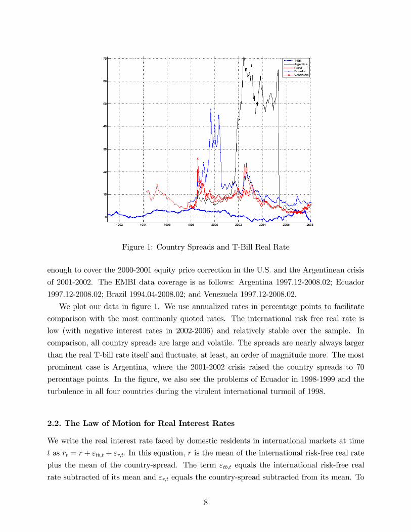
Figure 1: Country Spreads and T-Bill Real Rate

enough to cover the 2000-2001 equity price correction in the U.S. and the Argentinean crisis

of 2001-2002. The EMBI data coverage is as follows: Argentina 1997.12-2008.02; Ecuador

1997.12-2008.02; Brazil 1994.04-2008.02; and Venezuela 1997.12-2008.02.

We plot our data in �gure 1. We use annualized rates in percentage points to facilitate

comparison with the most commonly quoted rates. The international risk free real rate is

low (with negative interest rates in 2002-2006) and relatively stable over the sample. In

comparison, all country spreads are large and volatile. The spreads are nearly always larger

than the real T-bill rate itself and �uctuate, at least, an order of magnitude more. The most

prominent case is Argentina, where the 2001-2002 crisis raised the country spreads to 70

percentage points. In the �gure, we also see the problems of Ecuador in 1998-1999 and the

turbulence in all four countries during the virulent international turmoil of 1998.

2.2. The Law of Motion for Real Interest Rates

We write the real interest rate faced by domestic residents in international markets at time

t as rt = r + "tb;t + "r;t: In this equation, r is the mean of the international risk-free real rate

plus the mean of the country-spread. The term "tb;t equals the international risk-free real

rate subtracted of its mean and "r;t equals the country-spread subtracted from its mean. To

8

ease notation, we omit a subindex for the country-speci�c variables and parameters.

We specify that both "tb;t and "r;t follow AR(1) processes described by:

"tb;t = �tb"tb;t�1 + e�tb;tutb;t (1)

and:

"r;t = �r"r;t�1 + e�r;tur;t (2)

where both ur;t and utb;t are normally distributed shocks with mean zero and unit variance.

The main feature of our process is that the standard deviations �tb;t and �r;t are not constant,

as commonly assumed, but follow an AR(1) processes:

�tb;t =�1� ��tb

��tb + ��tb�tb;t�1 + �tbu�tb;t (3)

and

�r;t =�1� ��r

��r + ��r�r;t�1 + �ru�r;t (4)

where both u�r;t and u�tb;t are normally distributed shocks with mean zero and unit variance.

Thus, our process for interest rates displays stochastic volatility. The parameters �tb and �tbcontrol the degree of mean volatility and stochastic volatility in the international risk free

real rate: a high �tb implies a high mean volatility of the international risk free real rate and

a high �tb, a high degree of stochastic volatility. The same can be said about �r and �r and

the mean volatility and stochastic volatility in the country spread.

Our speci�cation is parsimonious yet powerful enough to capture some salient peculiarities

of the data (Shepard, 2008). Alternative speci�cations, like estimating realized volatility, are

of di¢ cult to implement because we do not have intraday data. Also, realized volatility is

less useful for us since we need a parametric law of motion for volatility to feed into the

equilibrium model of section 3.

Two shocks a¤ect each of the components of the real interest rate: one in�uencing its

level and another its volatility. For instance, the deviation due to the international risk-free

real rate, "tb;t, is hit by utb;t and u�tb;t. The �rst innovation, utb;t, changes the level of the

deviation, while the second innovation, u�tb;t, a¤ects the standard deviation of utb;t. The

shocks ur;t and u�r;t have a similar reading. We call utb;t and ur;t shocks to the level of the

international risk-free real rate and the country-spread, respectively.4 We call u�tb;t and u�r;tshocks to the volatility of international risk free real rate and the country spread, respectively.

4Strictly speaking, they are shocks to the deviation of the real interest rate with respect to its mean dueto the international risk-free rate and the country-spreads. Hereafter, to facilatate exposition, we omit theword �deviation�where we do not risk ambiguity.

9

Sometimes, for simplicity, we call this second type of innovation stochastic volatility shocks.

Following the literature, we can interpret a shock to the volatility of real interest rates from

at least two di¤erent perspectives. First, higher volatility may re�ect more risk surrounding

the world �nancial markets. Times generally understood as uncertain, such as the Asian and

the Long Term Capital Management (LTCM) crises, are associated with high volatility. A

second interpretation builds on the idea that volatility is related to information (Ross, 1989,

and Andersen, 1996). During turbulent times, news arrives frequently (or perhaps more

attention is devoted to it), inducing high volumes of trade in foreign debt and rising volatility

in interest rates.

As our benchmark exercise, we assume that utb;t; ur;t; u�tb;t; and u�r;t; are independent of

each other. How strong is this assumption? We checked that utb;t and ur;t are uncorrelated in

our data. This result con�rms the �ndings of Neumeyer and Perri (2005). At the same time,

we will report below that 1) the pair utb;t and u�tb;t is strongly correlated and 2) the pair

ur;t and u�r;t is strongly correlated as well. Motivated by this evidence, we will reestimate

our stochastic volatility process allowing for correlation. However, we keep the case without

correlation as our benchmark because it more neatly separates the e¤ects of the changes to

levels from the e¤ects of changes to volatility.

2.3. Estimation

We estimate the parameters of the process in equations (1) to (4) with a likelihood-based

approach. The likelihood of these processes is challenging to evaluate because of the presence

of two innovations, the innovation to levels and to volatility, that interact in a non-linear

way. We address this problem using the Particle �lter. This �lter is a Sequential Monte

Carlo algorithm that allows for the evaluation of the likelihood given some parameter values

through resampling simulation methods. The appendix o¤ers further details and references.

We follow a Bayesian approach to inference by combining the likelihood function with a prior.

In our context, Bayesian inference is convenient because we have short samples that can be

complemented with pre-sample information.

2.3.1. Priors

We now elicit our priors. We start by concentrating on the priors for the parameters driving

the law of motion of the country spread deviation. Then, we analyze the priors for the

parameters of the process for international risk-free real rate deviations.

10

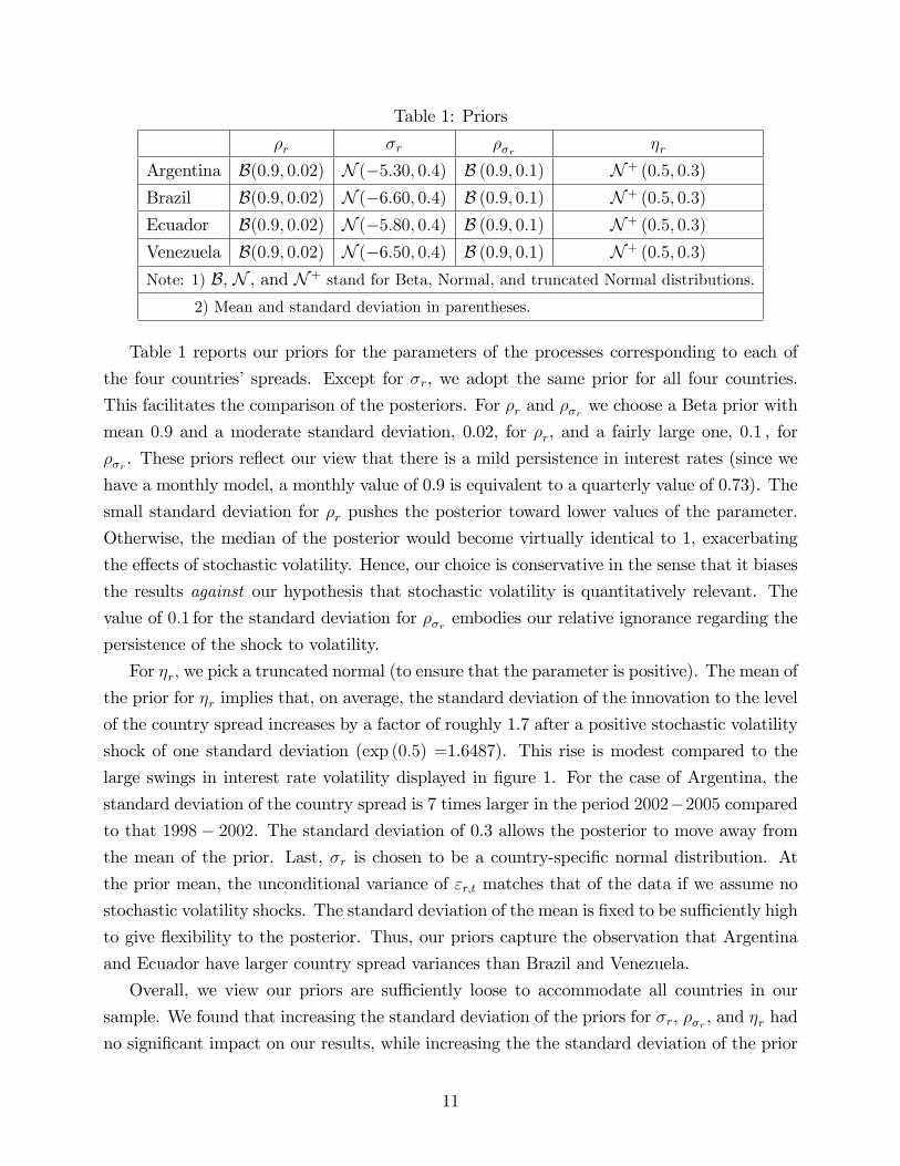
Table 1: Priors

�r �r ��r �r

Argentina B(0:9; 0:02) N (�5:30; 0:4) B (0:9; 0:1) N+ (0:5; 0:3)

Brazil B(0:9; 0:02) N (�6:60; 0:4) B (0:9; 0:1) N+ (0:5; 0:3)

Ecuador B(0:9; 0:02) N (�5:80; 0:4) B (0:9; 0:1) N+ (0:5; 0:3)

Venezuela B(0:9; 0:02) N (�6:50; 0:4) B (0:9; 0:1) N+ (0:5; 0:3)

Note: 1) B, N , and N+ stand for Beta, Normal, and truncated Normal distributions.

2) Mean and standard deviation in parentheses.

Table 1 reports our priors for the parameters of the processes corresponding to each of

the four countries�spreads. Except for �r, we adopt the same prior for all four countries.

This facilitates the comparison of the posteriors. For �r and ��r we choose a Beta prior with

mean 0:9 and a moderate standard deviation, 0.02, for �r, and a fairly large one, 0:1 , for

��r . These priors re�ect our view that there is a mild persistence in interest rates (since we

have a monthly model, a monthly value of 0.9 is equivalent to a quarterly value of 0.73). The

small standard deviation for �r pushes the posterior toward lower values of the parameter.

Otherwise, the median of the posterior would become virtually identical to 1, exacerbating

the e¤ects of stochastic volatility. Hence, our choice is conservative in the sense that it biases

the results against our hypothesis that stochastic volatility is quantitatively relevant. The

value of 0:1 for the standard deviation for ��r embodies our relative ignorance regarding the

persistence of the shock to volatility.

For �r; we pick a truncated normal (to ensure that the parameter is positive). The mean of

the prior for �r implies that, on average, the standard deviation of the innovation to the level

of the country spread increases by a factor of roughly 1.7 after a positive stochastic volatility

shock of one standard deviation (exp (0:5) =1.6487). This rise is modest compared to the

large swings in interest rate volatility displayed in �gure 1. For the case of Argentina, the

standard deviation of the country spread is 7 times larger in the period 2002�2005 comparedto that 1998 � 2002. The standard deviation of 0.3 allows the posterior to move away fromthe mean of the prior. Last, �r is chosen to be a country-speci�c normal distribution. At

the prior mean, the unconditional variance of "r;t matches that of the data if we assume no

stochastic volatility shocks. The standard deviation of the mean is �xed to be su¢ ciently high

to give �exibility to the posterior. Thus, our priors capture the observation that Argentina

and Ecuador have larger country spread variances than Brazil and Venezuela.

Overall, we view our priors are su¢ ciently loose to accommodate all countries in our

sample. We found that increasing the standard deviation of the priors for �r, ��r , and �r had

no signi�cant impact on our results, while increasing the the standard deviation of the prior

11

for �r favors our case. We further elaborate on the e¤ects of the priors on our quantitative

results in section 7.

The priors for the parameters of the law of motion of the international risk free real rate

are chosen following an identical approach than for the country speci�c spreads. Thus, the

justi�cations we provided before for these priors also hold here. We choose Beta priors for

�tb and ��tb with mean 0:9 and standard deviations of 0.02 and 0.1 respectively. For �tb; we

picked a truncated normal with mean 0:5 and standard deviation 0.3. Finally, �tb is such

that, at the prior mean, �8, the unconditional variance of "tb;t matches the one observed inthe data without stochastic volatility shocks. The standard deviation of the prior of �tb is

0.4, a 5 percent of the mean.

2.3.2. Posterior Estimates

We draw 20,000 times from the posterior of each of the �ve processes that we estimate (one

for the international risk-free real rate and one for each country spread) using a random

walk Metropolis-Hastings. The draw was run after an exhaustive search for appropriate

initial conditions and an additional 5,000 burn-in draws. We select the scaling matrix of

the proposal density to induce the appropriate acceptance ratio of proposals (Roberts et al.,

1997). Each evaluation of the likelihood is performed with 2,000 particles. We implemented

standard tests of convergence of the simulations, both of the Metropolis-Hastings and of the

Particle �lter. Given the low dimensionality of the problem, even a relatively short draw like

ours converges without further problems.

The sample mean for the real return of the T-bill, our measure of the international risk-

free real interest rate, is 0.001, a number that coincides, for example, with Campbell (2003).

Table 2 presents the mean of the monthly real interest rate for each country, r. Each of

them pays a considerable risk premium, from the 0.007 of Brazil and Venezuela to the 0.02

of Argentina. In annualized terms, the mean di¤erential varies from 840 to 2400 basis points.

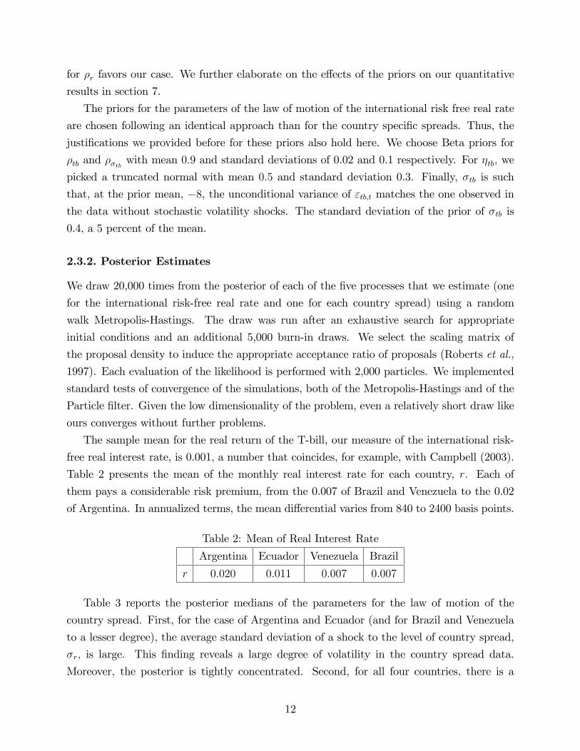
Table 2: Mean of Real Interest Rate

Argentina Ecuador Venezuela Brazil

r 0:020 0:011 0:007 0:007

Table 3 reports the posterior medians of the parameters for the law of motion of the

country spread. First, for the case of Argentina and Ecuador (and for Brazil and Venezuela

to a lesser degree), the average standard deviation of a shock to the level of country spread,

�r; is large. This �nding reveals a large degree of volatility in the country spread data.

Moreover, the posterior is tightly concentrated. Second, for all four countries, there is a

12

substantial presence of stochastic volatility in the country spread series (a large �r). The

shocks to the level and standard deviation of the country spread are highly persistent (large

�r and ��r). The standard deviation of the posteriors of �r is small (the 95 percent probability

sets are entirely above 0.9). The standard deviation of the posteriors of ��r is larger, but

even at the 2.5 percentile, the persistence of the process in the range of 0.77 to 0.99.

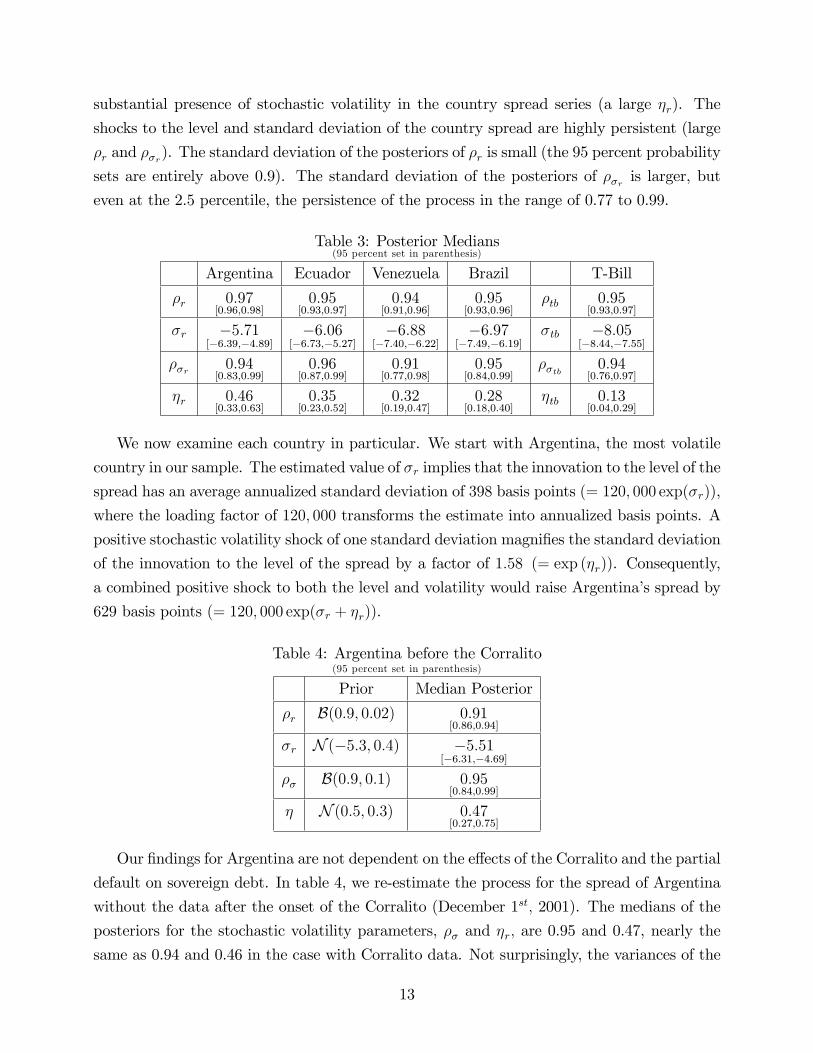
Table 3: Posterior Medians(95 percent set in parenthesis)

Argentina Ecuador Venezuela Brazil T-Bill

�r 0:97[0:96;0:98]

0:95[0:93;0:97]

0:94[0:91;0:96]

0:95[0:93;0:96]

�tb 0:95[0:93;0:97]

�r �5:71[�6:39;�4:89]

�6:06[�6:73;�5:27]

�6:88[�7:40;�6:22]

�6:97[�7:49;�6:19]

�tb �8:05[�8:44;�7:55]

��r 0:94[0:83;0:99]

0:96[0:87;0:99]

0:91[0:77;0:98]

0:95[0:84;0:99]

��tb 0:94[0:76;0:97]

�r 0:46[0:33;0:63]

0:35[0:23;0:52]

0:32[0:19;0:47]

0:28[0:18;0:40]

�tb 0:13[0:04;0:29]

We now examine each country in particular. We start with Argentina, the most volatile

country in our sample. The estimated value of �r implies that the innovation to the level of the

spread has an average annualized standard deviation of 398 basis points (= 120; 000 exp(�r)),

where the loading factor of 120; 000 transforms the estimate into annualized basis points. A

positive stochastic volatility shock of one standard deviation magni�es the standard deviation

of the innovation to the level of the spread by a factor of 1:58 (= exp (�r)). Consequently,

a combined positive shock to both the level and volatility would raise Argentina�s spread by

629 basis points (= 120; 000 exp(�r + �r)).

Table 4: Argentina before the Corralito(95 percent set in parenthesis)

Prior Median Posterior

�r B(0:9; 0:02) 0:91[0:86;0:94]

�r N (�5:3; 0:4) �5:51[�6:31;�4:69]

�� B(0:9; 0:1) 0:95[0:84;0:99]

� N (0:5; 0:3) 0:47[0:27;0:75]

Our �ndings for Argentina are not dependent on the e¤ects of the Corralito and the partial

default on sovereign debt. In table 4, we re-estimate the process for the spread of Argentina

without the data after the onset of the Corralito (December 1st; 2001). The medians of the

posteriors for the stochastic volatility parameters, �� and �r; are 0.95 and 0.47, nearly the

same as 0.94 and 0.46 in the case with Corralito data. Not surprisingly, the variances of the

13

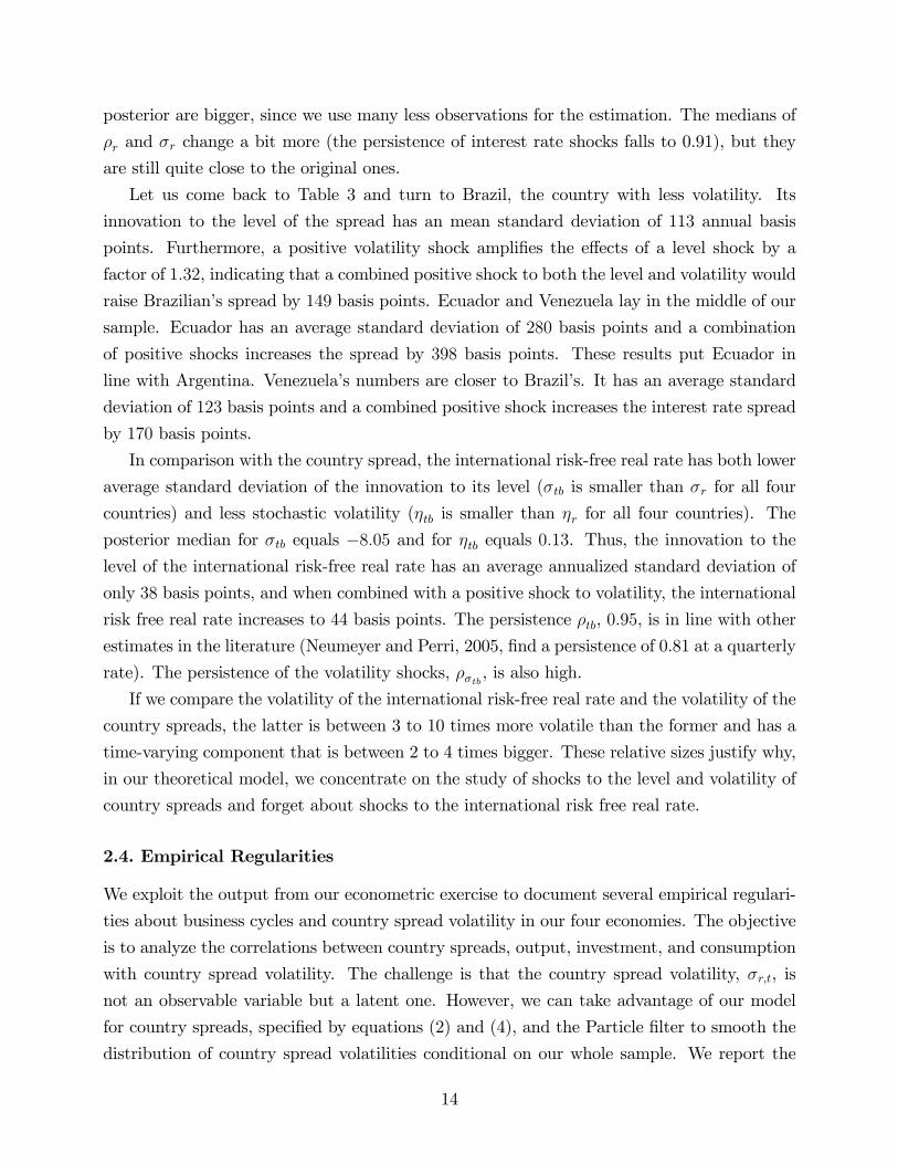
posterior are bigger, since we use many less observations for the estimation. The medians of

�r and �r change a bit more (the persistence of interest rate shocks falls to 0.91), but they

are still quite close to the original ones.

Let us come back to Table 3 and turn to Brazil, the country with less volatility. Its

innovation to the level of the spread has an mean standard deviation of 113 annual basis

points. Furthermore, a positive volatility shock ampli�es the e¤ects of a level shock by a

factor of 1:32, indicating that a combined positive shock to both the level and volatility would

raise Brazilian�s spread by 149 basis points. Ecuador and Venezuela lay in the middle of our

sample. Ecuador has an average standard deviation of 280 basis points and a combination

of positive shocks increases the spread by 398 basis points. These results put Ecuador in

line with Argentina. Venezuela�s numbers are closer to Brazil�s. It has an average standard

deviation of 123 basis points and a combined positive shock increases the interest rate spread

by 170 basis points.

In comparison with the country spread, the international risk-free real rate has both lower

average standard deviation of the innovation to its level (�tb is smaller than �r for all four

countries) and less stochastic volatility (�tb is smaller than �r for all four countries). The

posterior median for �tb equals �8:05 and for �tb equals 0:13. Thus, the innovation to thelevel of the international risk-free real rate has an average annualized standard deviation of

only 38 basis points, and when combined with a positive shock to volatility, the international

risk free real rate increases to 44 basis points. The persistence �tb, 0:95, is in line with other

estimates in the literature (Neumeyer and Perri, 2005, �nd a persistence of 0.81 at a quarterly

rate). The persistence of the volatility shocks, ��tb, is also high.

If we compare the volatility of the international risk-free real rate and the volatility of the

country spreads, the latter is between 3 to 10 times more volatile than the former and has a

time-varying component that is between 2 to 4 times bigger. These relative sizes justify why,

in our theoretical model, we concentrate on the study of shocks to the level and volatility of

country spreads and forget about shocks to the international risk free real rate.

2.4. Empirical Regularities

We exploit the output from our econometric exercise to document several empirical regulari-

ties about business cycles and country spread volatility in our four economies. The objective

is to analyze the correlations between country spreads, output, investment, and consumption

with country spread volatility. The challenge is that the country spread volatility, �r;t, is

not an observable variable but a latent one. However, we can take advantage of our model

for country spreads, speci�ed by equations (2) and (4), and the Particle �lter to smooth the

distribution of country spread volatilities conditional on our whole sample. We report the

14

value of the average smoothed volatility conditional on the median of the posterior of the

parameters. Since we use monthly data for interest rates and quarterly data for aggregate

variables, we linearly interpolate output, investment, and consumption.

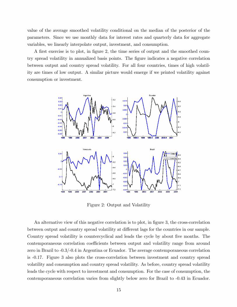
A �rst exercise is to plot, in �gure 2, the time series of output and the smoothed coun-

try spread volatility in annualized basis points. The �gure indicates a negative correlation

between output and country spread volatility. For all four countries, times of high volatil-

ity are times of low output. A similar picture would emerge if we printed volatility against

consumption or investment.

Figure 2: Output and Volatility

An alternative view of this negative correlation is to plot, in �gure 3, the cross-correlation

between output and country spread volatility at di¤erent lags for the countries in our sample.

Country spread volatility is countercyclical and leads the cycle by about �ve months. The

contemporaneous correlation coe¢ cients between output and volatility range from around

zero in Brazil to -0.3/-0.4 in Argentina or Ecuador. The average contemporaneous correlation

is -0.17. Figure 3 also plots the cross-correlation between investment and country spread

volatility and consumption and country spread volatility. As before, country spread volatility

leads the cycle with respect to investment and consumption. For the case of consumption, the

contemporaneous correlation varies from slightly below zero for Brazil to -0.43 in Ecuador.

15

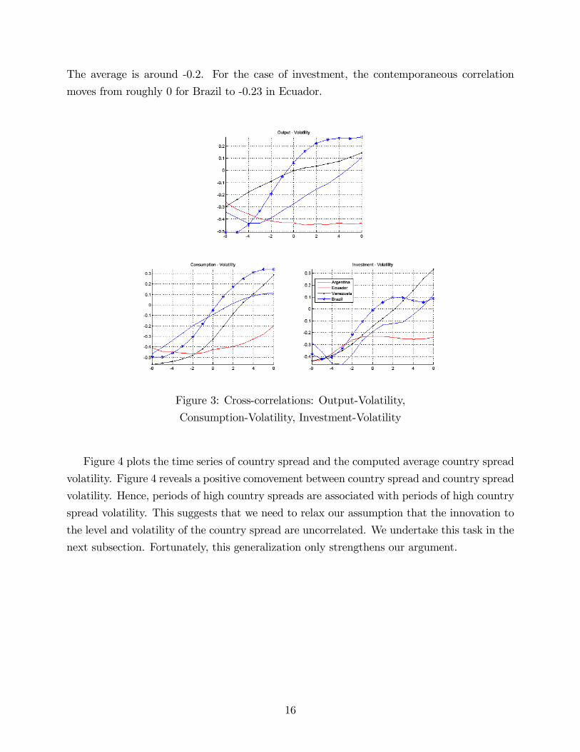
The average is around -0.2. For the case of investment, the contemporaneous correlation

moves from roughly 0 for Brazil to -0.23 in Ecuador.

Figure 3: Cross-correlations: Output-Volatility,

Consumption-Volatility, Investment-Volatility

Figure 4 plots the time series of country spread and the computed average country spread

volatility. Figure 4 reveals a positive comovement between country spread and country spread

volatility. Hence, periods of high country spreads are associated with periods of high country

spread volatility. This suggests that we need to relax our assumption that the innovation to

the level and volatility of the country spread are uncorrelated. We undertake this task in the

next subsection. Fortunately, this generalization only strengthens our argument.

16

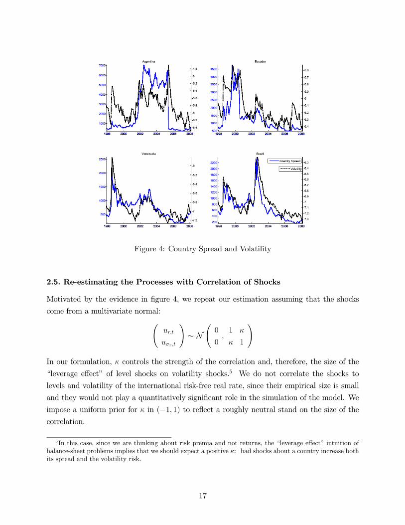
Figure 4: Country Spread and Volatility

2.5. Re-estimating the Processes with Correlation of Shocks

Motivated by the evidence in �gure 4, we repeat our estimation assuming that the shocks

come from a multivariate normal: ur;t

u�r;t

!� N

0

0;1 �

� 1

!

In our formulation, � controls the strength of the correlation and, therefore, the size of the

�leverage e¤ect� of level shocks on volatility shocks.5 We do not correlate the shocks to

levels and volatility of the international risk-free real rate, since their empirical size is small

and they would not play a quantitatively signi�cant role in the simulation of the model. We

impose a uniform prior for � in (�1; 1) to re�ect a roughly neutral stand on the size of thecorrelation:

5In this case, since we are thinking about risk premia and not returns, the �leverage e¤ect� intuition ofbalance-sheet problems implies that we should expect a positive �: bad shocks about a country increase bothits spread and the volatility risk.

17

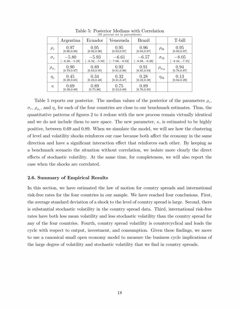
Table 5: Posterior Medians with Correlation(95 percent set in parenthesis)

Argentina Ecuador Venezuela Brazil T-bill

�r 0:97[0:96;0:98]

0:95[0:92;0:96]

0:95[0:93;0:97]

0:96[0:94;0:97]

�tb 0:95[0:93;0:97]

�r �5:80[�6:28;�5:28]

�5:93[�6:32;�5:50]

�6:61[�7:00;�6:02]

�6:57[�6:88;�6:26]

�tb �8:05[�8:44;�7:55]

��r 0:90[0:79;0:97]

0:89[0:83;0:95]

0:92[0:81;0:96]

0:91[0:85;0:94]

��tb 0:94[0:76;0:97]

�r 0:45[0:28;0:65]

0:34[0:23;0:48]

0:32[0:21;0:47]

0:28[0:22;0:38]

�tb 0:13[0:04;0:29]

� 0:69[0:39;0:89]

0:89[0:75;96]

0:75[0:53;0:89]

0:89[0:76;0:95]

Table 5 reports our posterior. The median values of the posterior of the parameters �r;

�r; ��r ; and �r for each of the four countries are close to our benchmark estimates. Thus, the

quantitative patterns of �gures 2 to 4 redone with the new process remain virtually identical

and we do not include them to save space. The new parameter, �; is estimated to be highly

positive, between 0.69 and 0.89. When we simulate the model, we will see how the clustering

of level and volatility shocks reinforces our case because both a¤ect the economy in the same

direction and have a signi�cant interaction e¤ect that reinforces each other. By keeping as

a benchmark scenario the situation without correlation, we isolate more clearly the direct

e¤ects of stochastic volatility. At the same time, for completeness, we will also report the

case when the shocks are correlated.

2.6. Summary of Empirical Results

In this section, we have estimated the law of motion for country spreads and international

risk-free rates for the four countries in our sample. We have reached four conclusions. First,

the average standard deviation of a shock to the level of country spread is large. Second, there

is substantial stochastic volatility in the country spread data. Third, international risk-free

rates have both less mean volatility and less stochastic volatility than the country spread for

any of the four countries. Fourth, country spread volatility is countercyclical and leads the

cycle with respect to output, investment, and consumption. Given these �ndings, we move

to use a canonical small open economy model to measure the business cycle implications of

the large degree of volatility and stochastic volatility that we �nd in country spreads.

18

3. The Model

We formulate a prototypical small open economy with incomplete asset markets in the spirit

of Mendoza (1991), Correia et al. (1995), Neumeyer and Perri (2005), and Uribe and Yue

(2006). The small open economy is populated by a representative household whose preferences

are captured by the utility function:

E01Xt=0

�t[Ct � !�1H!

t ]1�v � 1

1� v: (5)

Here, E0 is the conditional expectations operator, Ct denotes consumption, Ht stands for

hours worked, and � 2 (0; 1) corresponds to the discount factor.Our choice of the Greenwood-Hercowitz-Hu¤man (GHH) preferences follows the �nding

by Correia et al. (1995) that such utility function is better suited to match the second

moments of small open economies. The main appealing feature of the GHH preferences is

the absence of wealth e¤ects on the labor supply decision. In this way, labor supply depends

only on the real wage, and the model, as suggested by the data, is capable of generating a

contraction in consumption, labor, and output after a positive shock to the interest rate level.

The real interest rate rt faced by domestic residents in �nancial markets follows equations

(1) to (4) speci�ed in section 2. This assumption, motivated by our empirical evidence, is

the main di¤erence of our model with respect to the standard small open economy business

cycle model.

The household can invest in two types of assets: the stock of physical capital, Kt, and

an internationally traded bond, Dt. We maintain the convention that positive values of Dt

denote debt. Then, the household�s budget constraint is given by:

Dt+1

1 + rt= Dt �WtHt �RtKt + Ct + It +

�D2(Dt+1 �D)2 (6)

whereWt represents the real wage, Rt denotes the real rental rate of capital, It is our notation

for gross domestic investment, �D > 0 is a parameter that controls the costs of holding a net

foreign asset position, and D is a parameter that determines average debt. The cost is paid

to some foreign international institution (for example, an investment bank that handles the

issuing of bonds for the representative household).

We highlight two points about (6). First, the household has access to a one-period, un-

contingent bond. This re�ects the extremely limited ability of the countries in our sample

to issue debt at long horizons; when they do so, it is only accepted by the market at steep

discounts. For a theoretical investigation of why this is so, see Alfaro and Kanczuk (forthcom-

19

ing) and Broner et al. (2007). Consequently, the household will not have the possibility of

structuring its debt maturity to minimize the e¤ects of volatility (or, equivalently, the market

for volatility contracts on the debt does not exist or it is too small.) Second, we assume that

the household faces this cost of holding a net foreign asset position with the purpose of elim-

inating the unit root otherwise built into the dynamics of the small open economy model.

This unit root is inconvenient because it makes it di¢ cult to analyze transient dynamics.

Section 7 will quantitatively compare our speci�cation with other ways to close the model.

The stock of capital evolves according to the law of motion:

Kt+1 = (1� �)Kt +

1� �

2

�ItIt�1

� 1�2!

It

where � is the depreciation rate and the process of capital accumulation is subject to ad-

justment costs. The parameter � > 0 controls the size of these adjustment costs. The

introduction of capital adjustment costs is commonplace in business cycle models of small

open economies. They are a convenient and plausible way to avoid excessive investment

volatility in response to changes in the real interest rate. The representative household is

also subject to the typical no-Ponzi-game condition.

Firms rent capital and labor from households to produce output in a competitive envi-

ronment according to the technology Yt = K�t

�eXtHt

�1��where Xt corresponds to a labor-

augmenting productivity shock that follows an AR(1) process:

Xt = �xXt�1 + e�xux;t (7)

where ux;t is a normally distributed shock with zero mean and variance equal to one.

Firms maximize pro�ts by equating wages and the rental rate of capital to marginal

productivities. Thus, we can rewrite equation (6) as:

NXt = Yt � Ct � It = Dt �Dt+1

1 + rt+�D2(Dt+1 �D)2

where NXt are net exports. Also, we can de�ne the current account as CAt = Dt � Dt+1

where the order of the terms is switched from conventional notation because positive values

of Dt denote debt. Combining the de�nitions of net exports and current account:

CAt = (1 + rt)NXt � rtDt � (1 + rt)�D2(Dt+1 �D)2

20

3.1. Equilibrium

A competitive equilibrium can be de�ned in a standard way as a sequence of allocations and

prices such that both the representative household and the �rm maximize and markets clear.

The set of equilibrium conditions that characterize the time paths for Ct; Dt+1; Kt+1, Ht;

and It are given by the �rst-order conditions for the household and the �rm:�Ct �

H!t

!

��v= �t; (8)

�t1 + rt

= �t�D (Dt+1 �D) + �Et�t+1; (9)

�'t + �Et�(1� �)'t+1 + �

Yt+1Kt+1

�t+1

�= 0; (10)

H!t = (1� �)Yt; (11)

't

"1� �

2

�It � It�1It�1

�2� �ItIt�1

�It � It�1It�1

�#+ �Et

"'t+1�

�It+1It

�2�It � It�1It�1

�#= �t (12)

together with the resource constraint, the law of motion for capital, the production function,

and the stochastic processes for the interest rate. The Lagrangian �t is associated with the

debt level and the Lagrangian 't with physical capital.

The deterministic steady state is given by the solution to the following set of equations:�C � H!

!

��v= �;

�

�(1� �)'+ �

Y

K�

�= ';

H!�1�C � H!

!

��v= (1� �)�

Y

H;

� = ';

D

1 + r= D � Y + C + I;

Y = K�H1��;

I = �K:

We will calibrate the value of D to ensure that the model generates an ergodic distribution

of debt with an average that matches the mean value of debt observed in the data. In addition,

r is set at the mean of the country�s real interest rate (T-bill plus EMBI). Hence, we have a

system of 7 equations for 7 unknowns: C; H; �; '; K; I; and Y .

21

3.2. Solving the Model

We solve the model by relying on perturbation methods to approximate the policy functions

of the agents and the laws of motion of exogenous variables around the deterministic steady

state de�ned above. Aruoba et al. (2006) report that perturbation methods are highly

accurate and deliver a fast solution in a closed economy version of the model considered

here.6

One of the exercises we are keenly interested in is to measure the e¤ects of a volatility

increase (a positive shock to either u�r;t or u�tb;t), while keeping the level of the real interest

rate unchanged (�xing ur;t = 0 and utb;t = 0). Consequently, we need to obtain a third

approximation of the policy functions. A �rst-order approximation to the model would miss

all of the dynamics induced by volatility because this approximation is certainty equivalent.

Thus, the policy functions would exclusively depend on the normally distributed shocks utb;t,

ur;t, and uX;t. Shocks to volatility, u�r;t and u�tb;t; do not appear in this approximation

(more precisely, the coe¢ cients in front of these variables are equal to zero). A second order

approximation would only capture the volatility e¤ect indirectly via cross product terms of

the form ur;tu�r;t and utb;tu�tb;t, that is, through the joint interaction of both shocks. Thus,

up to second order, volatility does not have an e¤ects as long as the real interest rate does not

change. It is only in a third-order approximation that the stochastic volatility shocks, u�;tand u�tb;t, enter as independent arguments in the policy functions with a coe¢ cient di¤erent

from zero. Hence, if we want to explore the direct role of volatility, we need to consider cubic

terms. Furthermore, given the estimated stochastic volatility processes, the cubic terms in

the policy functions are quantitatively signi�cant. This is one of the most relevant �ndings

of our paper. In the appendix, we show how the simulation paths of the model are a¤ected

by these higher order terms.

Also, the third-order approximation and our estimated stochastic processes move the

mean of the ergodic distributions of the endogenous variables of the model away from their

deterministic steady-state values. Thus, our calibration must target the moments of interest

generated by the ergodic distributions and not the moments of the deterministic steady state,

since those last ones are not representative of the stochastic dynamics.

There are two possible objections to our perturbation solution: �rst, whether approx-

imating the policy function around the steady state is the best choice; second, whether a

third-order solution is accurate enough. The �rst objection can be dealt with by observing

that 1) the approximation around the steady state is the asymptotically valid one (something

6Value function iteration or projection methods are too slow to run with the required level of accuracy(we have 8 state variables). Moreover, as we will see momentarily, the calibration of the model requires a fairamount of simulations. A slow solution method would make this task too onerous.

22

that cannot be said for sure about other approximation points) and that 2) the second order

terms include a constant that corrects for precautionary behavior. To answer the second

objection, we computed a sixth order approximation to the model. We found that the fourth,

�fth, and sixth order terms contributed next to nothing to the dynamics of interest.7 Once

you have the terms on volatility that the third order delivers, fourth and higher order terms

have extremely small coe¢ cients. Since the additional terms considerably slowed down the

solution and limited our ability to simulate and explore the model (in the sixth order we have

1,899,240 terms to compute), we stopped at the third order.

The states of the model are Statest =� bKt; bIt�1; bDt; Xt�1; "r;t�1; "tb;t�1; �r;t�1; �tb;t�1;�

�0and the exogenous shocks are �t = (uX;t; ur;t; utb;t; u�r;tu�tb;t)

0 ; where bKt; bIt�1; and bDt are

deviations of the logs of Kt and It�1; and the level of Dt with respect to the log of K and

I and the level of D (we do not take logs of D because it may be negative). Also, � is the

perturbation parameter.

We take a perturbation solution around � = 0, that is, around the steady state implied

when all the variances of the shocks are equal to zero. Since the optimal decision rules

depend on the states and the exogenous shocks, we de�ne st = (States0t; �0t)0 as the vector

of arguments of the policy function. Also, we call sit to the i � th entry of st and ns to the

cardinality of st. Thus, we can write the third-order approximation to the laws of motion of

the endogenous states. First, we have a law of motion for capital:

bKt+1 = Ki sit +

1

2 Ki;js

itsjt +

1

6 Ki;j;ls

itsjtslt;

where each term Ki;::: is a scalar and where we have followed the tensor notation:

Ki sit =

nsXi=1

Ki sit

Ki;jsitsjt =

nsXi=1

nsXi=1

Ki;jsitsjt

and

Ki;j;lsitsjtslt =

nsXi=1

nsXj=1

nsXl=1

Ki;j;lsitsjtslt

that eliminates the symbolPns

i=1 when no confusion arises. Similarly, we have a law of motion

7We want to be careful here. We found that for our calibration and estimated processes, these higherorders were not important. There might exist parameter values for which these orders are relevant.

23

of investment and foreign debt:

bIt = Ii sit +

1

2 Ii;js

itsjt +

1

6 Ii;j;ls

itsjtslt;bDt = Di s

it +

1

2 Di;js

itsjt +

1

6 Di;j;ls

itsjtslt

Finally, we have the law of motion for the technology shock, (7), the deviation of the

real interest rate due to the country spread, (2), the deviation of the real interest rate due

to the international risk-free real rate, (1), and the volatilities, (3) and (4). For the case of

the law of motion for the deviation of the real interest rate due to the country spread, (2),

and the deviation of the real interest rate due to the international risk-free real rate, (1),

we also consider third-order approximations instead of their exact form to keep the order of

the approximation consistent across equations. Our solution, including calculating all the

analytic derivatives, is implemented in Mathematica.

3.3. Calibration

We calibrate eight versions of the model, two for each country, one using our benchmark

estimates of the law of motion for interest rates (without correlation of the shocks to level

and volatility), and one for the alternative estimates (with correlation). Thereafter, we will

call the �rst version of the model, the process without correlation of shocks, M1, and the

second version, where we feed in the processes with correlation, M2.8 Since the estimated

processes for the interest rate are monthly, we set one period in our model to be one month

and calibrate the parameters accordingly. Below, when we compare the moments of the model

with the moments of the data, we aggregate three periods of the model to create a quarter.

We �x the value of the following �ve parameters in all eight calibrations: 1) the parameter

that determines the elasticity of labor to wages, ! = 1:6; 2) the depreciation factor; � =

0:014; 3) the capital income share, � = 0:32; 4) the inverse of the elasticity of intertemporal

substitution, v = 2; 5) and �x = 0:95; the autoregressive of the productivity process. The

values for !, �, and v are those used in Mendoza (1991), Schmitt-Grohé and Uribe (2003), and

Aguiar and Gopinath (2007). The depreciation rate is taken from Neumeyer and Perri (2005),

who �nd this high value appropriate for Argentina. The absence of equivalent measures for

the other countries forces us to use Argentina�s depreciation rate across the eight di¤erent

versions of our model. The autoregressive process is more di¢ cult to pin down because of the

absence of good data on the Solow residual. Following the suggestion of Mendoza (1991), we

8Ideally, we would like to estimate the structural parameters of the model. However, the lack of reliablehigh-frequency data and the non-linear nature of our solution method make such an enterprise infeasible.

24

select a value slightly lower than the one commonly chosen for rich economies. We checked

that our results are robust to this choice by recalibrating and recomputing the model for

values of �x as low as 0 without �nding much di¤erence in the e¤ects of volatility shocks.

The rest of the parameters di¤er across each version of the model. First, we set the

parameters for the law of motion of the real interest rate equal to the median of the posterior

distributions reported in section 2. Second, we set the discount factor equal to the inverse of

the gross mean real interest rate of each country � = (1 + r)�1. Conditional on the previous

choices, we pick the last four parameters to match moments of the ergodic distribution of the

model with moments of the data. We select four moments in the data: 1) output volatility; 2)

the volatility of consumption relative to the volatility of output; 3) the volatility of investment

with respect to output; and 4) the ratio of net exports over output. The parameters are 1)

�x, the standard deviation of productivity shocks; 2) �, the adjustment cost of capital; 3) D,

the parameter that controls average value debt; and 4) the holding cost of debt, �D.

If we were using the steady state to calibrate the model, we could pick each parameter to

match almost independently each of the four moments of interest in the data (for example,

�x would nail down output volatility and D would determine the ratio of net exports over

output). In the ergodic distribution, in contrast, the moments are all a¤ected by a non-

linear combination of the parameters. Hence, moving one parameter to improve, say, the

�t of volatility of consumption relative to the volatility of output may worsen the �t of the

volatility of investment with respect to output. We �x this problem by minimizing a quadratic

form of the distance of the moments of the model with those of the moments of the data.

In addition, to discipline the exercise further, we pick only two levels of �D; one for the two

most volatile countries, Argentina and Ecuador, and another for Venezuela and Brazil that

is 50 percent of the �rst value. Our choices for �D are consistent with the values reported

in Uribe and Yue (2006). Their small value helps to close the model without signi�cantly

a¤ecting its dynamic properties.

The four empirical moments to be matched are reported in table 6 and they are based on

H-P �ltered quarterly data from the sources described in section 2. The row nx=y displays

the average of net exports as a percentage point of output. A positive value means that the

country is running a trade surplus.

25

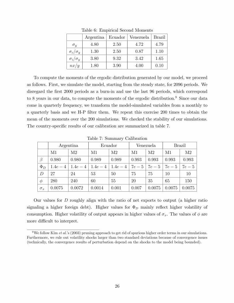
Table 6: Empirical Second Moments

Argentina Ecuador Venezuela Brazil

�y 4:80 2:50 4:72 4:79

�c=�y 1:30 2:50 0:87 1:10

�i=�y 3:80 9:32 3:42 1:65

nx=y 1:80 3:90 4:00 0:10

To compute the moments of the ergodic distribution generated by our model, we proceed

as follows. First, we simulate the model, starting from the steady state, for 2096 periods. We

disregard the �rst 2000 periods as a burn-in and use the last 96 periods, which correspond

to 8 years in our data, to compute the moments of the ergodic distribution.9 Since our data

come in quarterly frequency, we transform the model-simulated variables from a monthly to

a quarterly basis and we H-P �lter them. We repeat this exercise 200 times to obtain the

mean of the moments over the 200 simulations. We checked the stability of our simulations.

The country-speci�c results of our calibration are summarized in table 7.

Table 7: Summary Calibration

Argentina Ecuador Venezuela Brazil

M1 M2 M1 M2 M1 M2 M1 M2

� 0:980 0:980 0:989 0:989 0:993 0:993 0:993 0:993

�D 1:4e� 4 1:4e� 4 1:4e� 4 1:4e� 4 7e� 5 7e� 5 7e� 5 7e� 5D 27 24 53 50 75 75 10 10

� 280 240 60 55 20 35 65 150

�x 0:0075 0:0072 0:0014 0:001 0:007 0:0075 0:0075 0:0075

Our values for D roughly align with the ratio of net exports to output (a higher ratio

signaling a higher foreign debt). Higher values for �D mainly re�ect higher volatility of

consumption. Higher volatility of output appears in higher values of �x. The values of � are

more di¢ cult to interpret.

9We follow Kim et al.�s (2003) pruning approach to get rid of spurious higher order terms in our simulations.Furthermore, we rule out volatility shocks larger than two standard deviations because of convergence issues(technically, the convergence results of perturbation depend on the shocks to the model being bounded).

26

4. Results

In this section, we analyze the quantitative implications of our model. First, we report the

moments generated by the model and compare them with the data. Second, we look at the

impulse response functions (IRFs) of shocks to the level and volatility of country spreads.

Third, we decompose the variance of aggregate variables among di¤erent shocks.

4.1. Moments

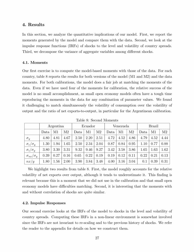
Our �rst exercise is to compute the model-based moments with those of the data. For each

country, table 8 reports the results for both versions of the model (M1 and M2) and the data

moments. For both calibrations, the model does a fair job at matching the moments of the

data. Even if we have used four of the moments for calibration, the relative success of the

model is no small accomplishment, as small open economy models often have a tough time

reproducing the moments in the data for any combination of parameter values. We found

it challenging to match simultaneously the volatility of consumption over the volatility of

output and the ratio of net exports-to-output, in particular for the Argentinean calibration.

Table 8: Second Moments

Argentina Ecuador Venezuela Brazil

Data M1 M2 Data M1 M2 Data M1 M2 Data M1 M2

�y 4:80 4:81 4:67 2:50 2:20 2:51 4:72 4:52 4:86 4:79 4:52 4:44

�c=�y 1:30 1:94 1:65 2:50 2:34 2:04 0:87 0:84 0:95 1:10 0:77 0:88

�i=�y 3:80 3:30 3:31 9:32 9:46 9:27 3:42 3:58 3:86 1:65 1:63 1:62

�nx=�y 0:39 0:27 0:16 0:65 0:22 0:19 0:19 0:12 0:11 0:22 0:21 0:13

nx=y 1:80 1:56 2:00 3:90 3:84 3:48 4:00 3:16 3:04 0:1 0:39 0:31

We highlight two results from table 8. First, the model roughly accounts for the relative

volatility of net exports over output, although it tends to underestimate it. This �nding is

relevant because this is a moment that we did not use in the calibration and that small open

economy models have di¢ culties matching. Second, it is interesting that the moments with

and without correlation of shocks are quite similar.

4.2. Impulse Responses

Our second exercise looks at the IRFs of the model to shocks in the level and volatility of

country spreads. Computing these IRFs in a non-linear environment is somewhat involved

since the IRFs are not invariant to re-scaling and to the previous history of shocks. We refer

the reader to the appendix for details on how we construct them.

27

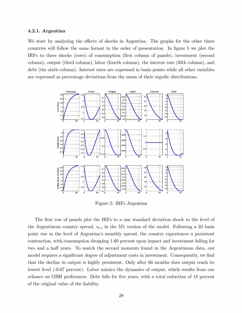
4.2.1. Argentina

We start by analyzing the e¤ects of shocks in Argentina. The graphs for the other three

countries will follow the same format in the order of presentation. In �gure 5 we plot the

IRFs to three shocks (rows) of consumption (�rst column of panels), investment (second

column), output (third column), labor (fourth column), the interest rate (�fth column), and

debt (the sixth column). Interest rates are expressed in basis points while all other variables

are expressed as percentage deviations from the mean of their ergodic distributions.

Figure 5: IRFs Argentina

The �rst row of panels plot the IRFs to a one standard deviation shock to the level of

the Argentinean country spread, ur;t in the M1 version of the model. Following a 33 basis

point rise in the level of Argentina�s monthly spread, the country experiences a persistent

contraction, with consumption dropping 1.60 percent upon impact and investment falling for

two and a half years. To match the second moments found in the Argentinean data, our

model requires a signi�cant degree of adjustment costs in investment. Consequently, we �nd

that the decline in output is highly persistent. Only after 66 months does output reach its

lowest level (-0.67 percent). Labor mimics the dynamics of output, which results from our

reliance on GHH preferences. Debt falls for �ve years, with a total reduction of 18 percent

of the original value of the liability.

28

The intuition for the drop in output, consumption, and investment is well understood

(see Neumeyer and Perri, 2005). A higher rt raises the service payment of the debt, reduces

consumption, forces a decrease in the level of debt (since now it is more costly to �nance

it), and lowers investment through a non-arbitrage condition between the returns to physical

capital and to foreign assets. We include this exercise to show that our model delivers the

same answers as the standard model when hit by equivalent level shocks and to place in

context the size of the IRFs to volatility shocks.

The contraction in economic activity may seem large relative to those found in the lit-

erature. Uribe and Yue (2006), for instance, estimate that a 1 percentage point rise in the

country spread reduces output by 0.15 percent and investment by 0.5 percent. However, we

must keep in mind that our time frame is a month, which implies that the interest rate in

fact rises by 4.1 percentage points on an annual basis. When we normalize the spread shock

so that the interest rate increases by 8.3 basis points upon impact (or 1 percentage point in a

yearly basis), consumption falls by 0.41 percent while output and investment contracts by 0.16

and 0.64 percent, respectively. These �ndings are more in line with the empirical estimates

reported by Uribe and Yue (2006). Furthermore, Uribe and Yue �nd that it takes about two

years for output to reach its lowest level. Their result raises the question of whether our

model may overpredict the persistence of output because of a large investment adjustment

cost. We will discuss the e¤ects of smaller adjustment costs in section 7.

The second row of panels plots the IRFs to a one standard deviation shock to the volatility

of the Argentinean country spread, u�;t. To put a shock of this size in perspective, our

econometric estimates of section 2 indicate the collapse of LTCM in 1998 meant a positive

volatility shock of 1.5 standard deviation and that the 2001 �nancial troubles amounted to

two repeated shocks of roughly 1 standard deviation.

This second row is one of the main points of our paper. First, note that there is no

movement on the level of the domestic interest rate faced by Argentina or its expected value.

Second, there is a) a contraction in monthly consumption (0:60 percent at impact), b) a

slow decrease of investment (after six quarters it falls 0:76 percent), c) a slow fall in output

(after four years, it falls 0.16 percent) and labor, and d) debt shrinks upon impact and keeps

declining until it reaches its lowest level (�10:21percent), roughly four years after the shock.These IRFs show how increments in risk have real e¤ects on the economy even when the level

of the real interest rate remains constant.

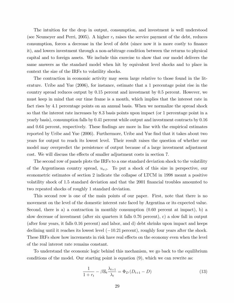
To understand the economic logic behind this mechanism, we go back to the equilibrium

conditions of the model. Our starting point is equation (9), which we can rewrite as:

1

1 + rt� �Et

�t+1�t

= �D (Dt+1 �D) (13)

29

A volatility shock leaves rt unchanged but it raises Et�t+1=�t; as illustrated in �gure 6. Why?The Lagrangian �t is the marginal utility of consumption. A higher real interest rate risk

causes more volatile consumption in the future. Our estimate for �r implies that a typical

stochastic volatility shock in Argentina raises the standard deviation of a shock to the level of

interest rates by a factor of 1.58 (= exp(�r)). Thus, households may face a 52 (1.58*33) basis

point surge in the monthly interest rates on their debt obligations if a one standard deviation

level shock to interest rate materializes tomorrow. Since marginal utility is convex, Jensen�s

inequality tells us that Et�t+1 rises. The total increment of the ratio Et�t+1=�t is smallerbecause, as we saw in the IRFs, consumption drops at impact and recovers in the following

periods, which increases marginal utility today and �t. In our calibration, this second e¤ect

is dominated by the dispersion of marginal utilities. Hence, the left-hand side of (13) falls

and we can make only the equation hold with equality if Dt+1 falls as well. The intuition

is that holding foreign debt is now riskier than before. Hence, the representative household

wants to reduce its exposure to this risk.10

Figure 6: Evolution of Et �t+1�t

10This argument is independent of technology shocks. Even with �x = 0, a volatility shock increases thedispersion of future marginal utilities through more dispersed real interest rate levels.

30

How can the representative household reduce its foreign debt? Since the country is not

more productive than before, the only way to do so is to increase net exports by either working

more or by reducing national absorption (the sum of consumption and investment). The �rst

alternative, working more, is precluded by our GHH utility function, since these preferences

do not have a wealth e¤ect. Hence, the household must reduce national absorption. This

can be done in three di¤erent ways; 1) consuming and investing less, 2) investing more and

consuming su¢ ciently less that national absorption falls, or 3) consuming more and investing

su¢ ciently less that national absorption falls. Option 3) does not smooth utility over time for

standard parameter values (although there are unrealistic combinations of parameter values

where they may be the optimal response).11 Option 2) is eliminated because, as we will show

below, investment must fall. Option 1) is, therefore, the only alternative.

To further understand why investment falls, we rewrite the Euler equation as:

�Et�(1� �) qt+1 +Rt+1

qt

�t+1�t

�= 1:

where we have de�ned the marginal cost of a unit of installed capital Kt+1 in terms of

consumption units as qt ='t�tand Rt is the rental rate of capital. Then:

�Et(1� �) qt+1 +Rt+1

qtEt�t+1�t

+ cov

�(1� �) qt+1 +Rt+1

qt;�t+1�t

�= 1

In this expression, the conditional covariance of the return to capital and the ratio of La-

grangians decreases when volatility rises. Households use debt to smooth productivity shocks.

Imagine that we are in a situation with low volatility. Then, after a negative shock to Xt

and the subsequent fall in the return to capital, consumption drops by a small amount (and

hence the ratio of Lagrangians rises by a small amount) because debt increases to smooth

consumption. However, when volatility is high, the household accepts a bigger reduction in

consumption after a productivity shock, since increasing the debt level carries a large interest

rate risk. At the same time, we just saw that Et�t+1=�t increases only by a small amountbecause of the interaction of mean-reverting consumption with the increased dispersion of

marginal utilities. Therefore, the only term that can change in our previous equation to

accommodate the lower covariance is to raise the term Et ((1� �) qt+1 +Rt+1) =qt: This goal

is accomplished with a lower investment today.12

11In the absence of adjustment costs, investment still falls but consumption increases at impact. However,without adjustment costs, the model does very poorly accounting for the moments of the data.12In comparison with the behavior of Et�t+1=�t, the fall of investment requires either a positive standard

deviation of the productivity shock and/or adjustment costs. If none of these mechanism is present, thereturn to capital is risk-free and the covariance is zero.

31

A slightly di¤erent way to understand the fall in investment after a volatility shock is

to note that foreign debt allows the household to hedge against the risk of holding physical

capital. This hedging property raises the desired level of physical capital. The total e¤ect is,

however, small because debt also allows the representative household to rely less on physical

capital as a self-insurance device. In calibration M1 for Argentina, the presence of debt

increases the average holdings of capital by 1.25 percent in comparison with a closed economy

version of our model. A higher volatility of the real interest rate makes the hedge provided by

foreign debt less attractive, it induces the household to reduce its level of debt, and, hence,

it also lowers its holdings of physical capital with a fall in investment.

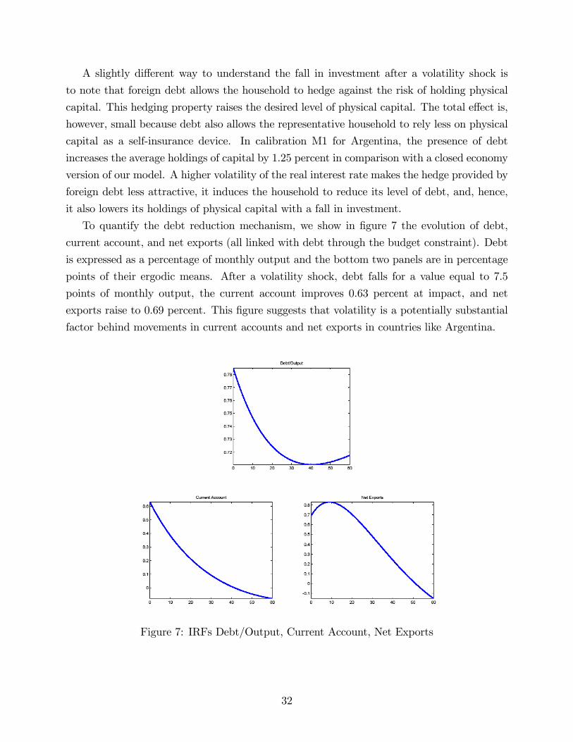
To quantify the debt reduction mechanism, we show in �gure 7 the evolution of debt,

current account, and net exports (all linked with debt through the budget constraint). Debt

is expressed as a percentage of monthly output and the bottom two panels are in percentage

points of their ergodic means. After a volatility shock, debt falls for a value equal to 7.5

points of monthly output, the current account improves 0.63 percent at impact, and net

exports raise to 0.69 percent. This �gure suggests that volatility is a potentially substantial

factor behind movements in current accounts and net exports in countries like Argentina.

Figure 7: IRFs Debt/Output, Current Account, Net Exports

32

The last row in �gure 5 plots the IRFs in the M2 version of the model where there is

correlation in the shocks to the level and volatility of rt: In this row, we plot the IRFs after

a one standard deviation level shock that is accompanied by a ��standard deviation shockto volatility. The pattern of the IRFs is qualitatively the same as in the �rst row. The

quantitative size is now bigger as we combine two shocks. The lesson from this third row is

that our results are robust to the correlation between shocks to the level and volatility of rt:

If anything, they become larger because of the interaction e¤ects of the two shocks.

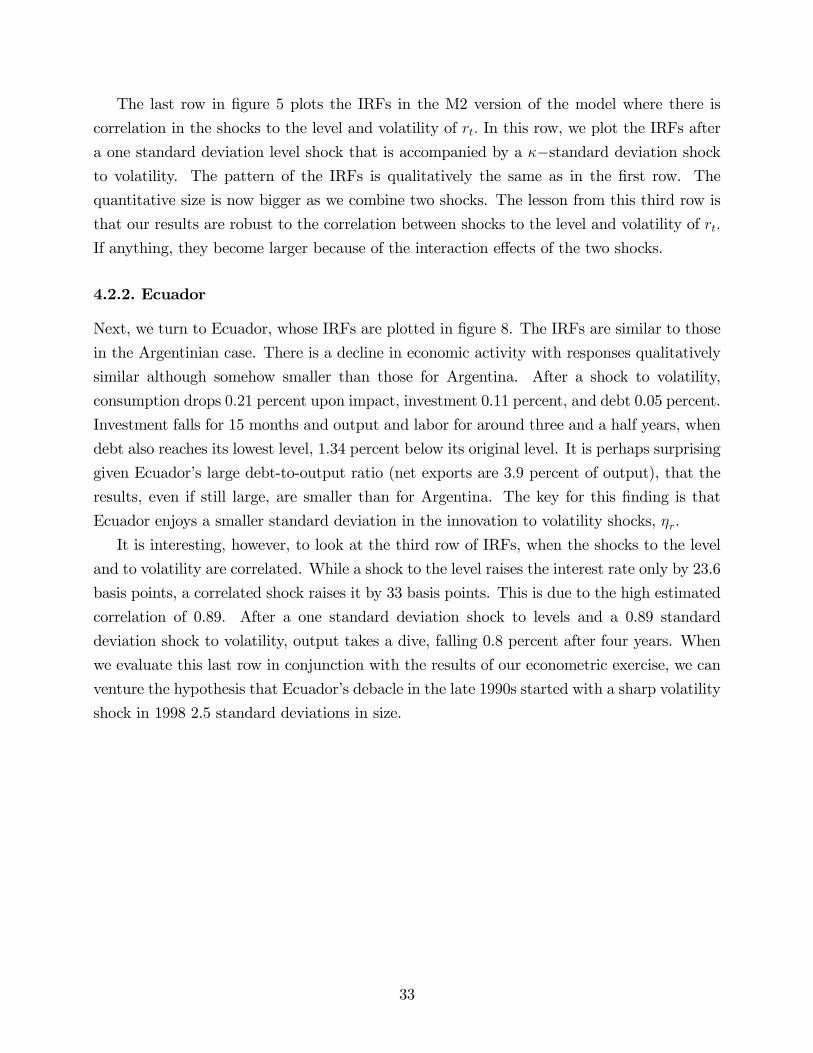
4.2.2. Ecuador

Next, we turn to Ecuador, whose IRFs are plotted in �gure 8. The IRFs are similar to those

in the Argentinian case. There is a decline in economic activity with responses qualitatively

similar although somehow smaller than those for Argentina. After a shock to volatility,

consumption drops 0:21 percent upon impact, investment 0.11 percent, and debt 0.05 percent.

Investment falls for 15 months and output and labor for around three and a half years, when

debt also reaches its lowest level, 1.34 percent below its original level. It is perhaps surprising

given Ecuador�s large debt-to-output ratio (net exports are 3:9 percent of output), that the

results, even if still large, are smaller than for Argentina. The key for this �nding is that

Ecuador enjoys a smaller standard deviation in the innovation to volatility shocks, �r.

It is interesting, however, to look at the third row of IRFs, when the shocks to the level

and to volatility are correlated. While a shock to the level raises the interest rate only by 23.6

basis points, a correlated shock raises it by 33 basis points. This is due to the high estimated

correlation of 0.89. After a one standard deviation shock to levels and a 0.89 standard

deviation shock to volatility, output takes a dive, falling 0.8 percent after four years. When

we evaluate this last row in conjunction with the results of our econometric exercise, we can

venture the hypothesis that Ecuador�s debacle in the late 1990s started with a sharp volatility

shock in 1998 2.5 standard deviations in size.

33

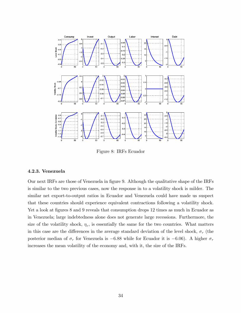
Figure 8: IRFs Ecuador

4.2.3. Venezuela

Our next IRFs are those of Venezuela in �gure 9. Although the qualitative shape of the IRFs

is similar to the two previous cases, now the response in to a volatility shock is milder. The

similar net export-to-output ratios in Ecuador and Venezuela could have made us suspect

that these countries should experience equivalent contractions following a volatility shock.

Yet a look at �gures 8 and 9 reveals that consumption drops 12 times as much in Ecuador as

in Venezuela; large indebtedness alone does not generate large recessions. Furthermore, the

size of the volatility shock, �r, is essentially the same for the two countries. What matters

in this case are the di¤erences in the average standard deviation of the level shock, �r (the

posterior median of �r for Venezuela is �6:88 while for Ecuador it is �6:06). A higher �rincreases the mean volatility of the economy and, with it, the size of the IRFs.

34

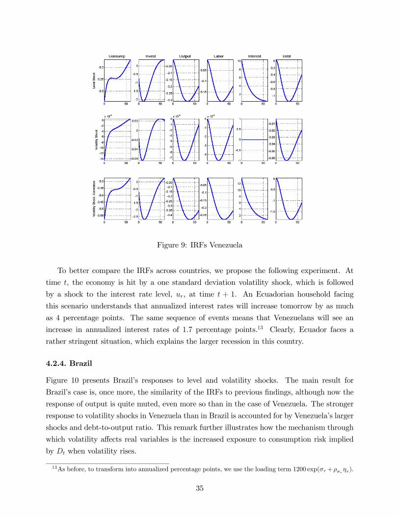
Figure 9: IRFs Venezuela

To better compare the IRFs across countries, we propose the following experiment. At

time t, the economy is hit by a one standard deviation volatility shock, which is followed

by a shock to the interest rate level, ur, at time t + 1. An Ecuadorian household facing

this scenario understands that annualized interest rates will increase tomorrow by as much

as 4 percentage points. The same sequence of events means that Venezuelans will see an

increase in annualized interest rates of 1:7 percentage points.13 Clearly, Ecuador faces a

rather stringent situation, which explains the larger recession in this country.

4.2.4. Brazil

Figure 10 presents Brazil�s responses to level and volatility shocks. The main result for

Brazil�s case is, once more, the similarity of the IRFs to previous �ndings, although now the

response of output is quite muted, even more so than in the case of Venezuela. The stronger

response to volatility shocks in Venezuela than in Brazil is accounted for by Venezuela�s larger

shocks and debt-to-output ratio. This remark further illustrates how the mechanism through

which volatility a¤ects real variables is the increased exposure to consumption risk implied

by Dt when volatility rises.

13As before, to transform into annualized percentage points, we use the loading term 1200 exp(�r+��r�r).

35

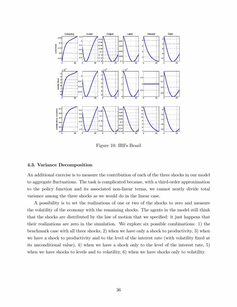
Figure 10: IRFs Brazil

4.3. Variance Decomposition

An additional exercise is to measure the contribution of each of the three shocks in our model

to aggregate �uctuations. The task is complicated because, with a third-order approximation

to the policy function and its associated non-linear terms, we cannot neatly divide total

variance among the three shocks as we would do in the linear case.

A possibility is to set the realizations of one or two of the shocks to zero and measure

the volatility of the economy with the remaining shocks. The agents in the model still think

that the shocks are distributed by the law of motion that we speci�ed: it just happens that

their realizations are zero in the simulation. We explore six possible combinations: 1) the

benchmark case with all three shocks, 2) when we have only a shock to productivity, 3) when

we have a shock to productivity and to the level of the interest rate (with volatility �xed at

its unconditional value), 4) when we have a shock only to the level of the interest rate, 5)

when we have shocks to levels and to volatility, 6) when we have shocks only to volatility.

36

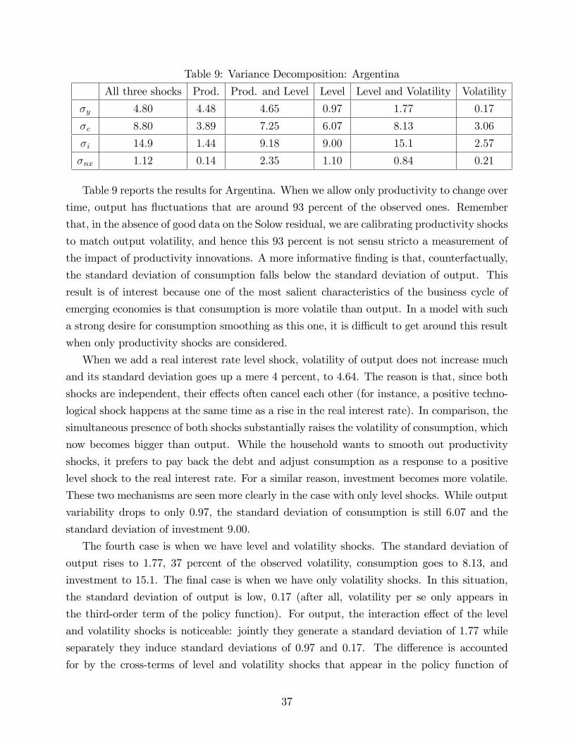
Table 9: Variance Decomposition: Argentina

All three shocks Prod. Prod. and Level Level Level and Volatility Volatility

�y 4:80 4:48 4:65 0:97 1:77 0:17

�c 8:80 3:89 7:25 6:07 8:13 3:06

�i 14:9 1:44 9:18 9:00 15:1 2:57

�nx 1:12 0:14 2:35 1:10 0:84 0:21

Table 9 reports the results for Argentina. When we allow only productivity to change over

time, output has �uctuations that are around 93 percent of the observed ones. Remember

that, in the absence of good data on the Solow residual, we are calibrating productivity shocks

to match output volatility, and hence this 93 percent is not sensu stricto a measurement of

the impact of productivity innovations. A more informative �nding is that, counterfactually,

the standard deviation of consumption falls below the standard deviation of output. This

result is of interest because one of the most salient characteristics of the business cycle of

emerging economies is that consumption is more volatile than output. In a model with such

a strong desire for consumption smoothing as this one, it is di¢ cult to get around this result

when only productivity shocks are considered.

When we add a real interest rate level shock, volatility of output does not increase much

and its standard deviation goes up a mere 4 percent, to 4.64. The reason is that, since both

shocks are independent, their e¤ects often cancel each other (for instance, a positive techno-

logical shock happens at the same time as a rise in the real interest rate). In comparison, the

simultaneous presence of both shocks substantially raises the volatility of consumption, which

now becomes bigger than output. While the household wants to smooth out productivity

shocks, it prefers to pay back the debt and adjust consumption as a response to a positive

level shock to the real interest rate. For a similar reason, investment becomes more volatile.

These two mechanisms are seen more clearly in the case with only level shocks. While output

variability drops to only 0.97, the standard deviation of consumption is still 6.07 and the

standard deviation of investment 9.00.

The fourth case is when we have level and volatility shocks. The standard deviation of

output rises to 1.77, 37 percent of the observed volatility, consumption goes to 8.13, and

investment to 15.1. The �nal case is when we have only volatility shocks. In this situation,

the standard deviation of output is low, 0.17 (after all, volatility per se only appears in

the third-order term of the policy function). For output, the interaction e¤ect of the level

and volatility shocks is noticeable: jointly they generate a standard deviation of 1.77 while

separately they induce standard deviations of 0.97 and 0.17. The di¤erence is accounted

for by the cross-terms of level and volatility shocks that appear in the policy function of

37

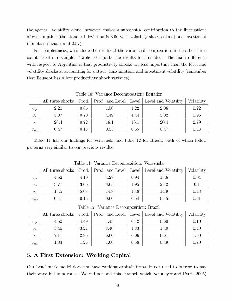
the agents. Volatility alone, however, makes a substantial contribution to the �uctuations

of consumption (the standard deviation is 3.06 with volatility shocks alone) and investment

(standard deviation of 2.57).

For completeness, we include the results of the variance decomposition in the other three

countries of our sample. Table 10 reports the results for Ecuador. The main di¤erence

with respect to Argentina is that productivity shocks are less important than the level and

volatility shocks at accounting for output, consumption, and investment volatility (remember

that Ecuador has a low productivity shock variance).

Table 10: Variance Decomposition: Ecuador

All three shocks Prod. Prod. and Level Level Level and Volatility Volatility

�y 2:20 0:86 1:50 1:22 2:06 0:22

�c 5:07 0:70 4:49 4:44 5:02 0:96

�i 20:4 0:72 16:1 16:1 20:4 2:79

�nx 0:47 0:13 0:55 0:55 0:47 0:43

Table 11 has our �ndings for Venezuela and table 12 for Brazil, both of which follow

patterns very similar to our previous results.

Table 11: Variance Decomposition: Venezuela

All three shocks Prod. Prod. and Level Level Level and Volatility Volatility

�y 4:52 4:19 4:28 0:94 1:46 0:04

�c 3:77 3:06 3:65 1:95 2:12 0:1

�i 15:5 5:08 14:8 13:8 14:9 0:43

�nx 0:47 0:18 0:60 0:54 0:45 0:31

Table 12: Variance Decomposition: Brazil

All three shocks Prod. Prod. and Level Level Level and Volatility Volatility

�y 4:52 4:49 4:43 0:42 0:60 0:10

�c 3:46 3:21 3:40 1:33 1:40 0:40

�i 7:11 2:95 6:60 6:06 6:61 1:50

�nx 1:33 1:26 1:60 0:58 0:49 0:70

5. A First Extension: Working Capital

Our benchmark model does not have working capital: �rms do not need to borrow to pay

their wage bill in advance. We did not add this channel, which Neumeyer and Perri (2005)

38

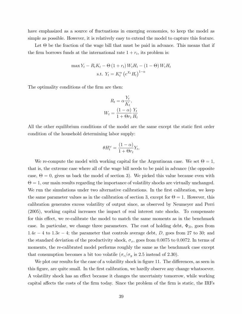
have emphasized as a source of �uctuations in emerging economies, to keep the model as

simple as possible. However, it is relatively easy to extend the model to capture this feature.

Let � be the fraction of the wage bill that must be paid in advance. This means that if

the �rm borrows funds at the international rate 1 + rt, its problem is:

maxYt �RtKt ��(1 + rt)WtHt � (1��)WtHt

s.t. Yt = K�t

�eXtHt

�1��The optimality conditions of the �rm are then:

Rt = �YtKt

;

Wt =(1� �)

1 + �rt

YtHt

All the other equilibrium conditions of the model are the same except the static �rst order

condition of the household determining labor supply:

�H!t =

(1� �)

1 + �rtYt;

We re-compute the model with working capital for the Argentinean case. We set � = 1,

that is, the extreme case where all of the wage bill needs to be paid in advance (the opposite

case, � = 0, gives us back the model of section 3). We picked this value because even with

� = 1, our main results regarding the importance of volatility shocks are virtually unchanged.

We run the simulations under two alternative calibrations. In the �rst calibration, we keep

the same parameter values as in the calibration of section 3, except for � = 1. However, this

calibration generates excess volatility of output since, as observed by Neumeyer and Perri

(2005), working capital increases the impact of real interest rate shocks. To compensate

for this e¤ect, we re-calibrate the model to match the same moments as in the benchmark

case. In particular, we change three parameters. The cost of holding debt, �D, goes from

1:4e � 4 to 1:3e � 4; the parameter that controls average debt, D; goes from 27 to 30; and

the standard deviation of the productivity shock, �x, goes from 0:0075 to 0:0072: In terms of

moments, the re-calibrated model performs roughly the same as the benchmark case except

that consumption becomes a bit too volatile (�c=�y is 2.5 instead of 2.30).

We plot our results for the case of a volatility shock in �gure 11. The di¤erences, as seen in

this �gure, are quite small. In the �rst calibration, we hardly observe any change whatsoever.

A volatility shock has an e¤ect because it changes the uncertainty tomorrow, while working

capital a¤ects the costs of the �rm today. Since the problem of the �rm is static, the IRFs

39

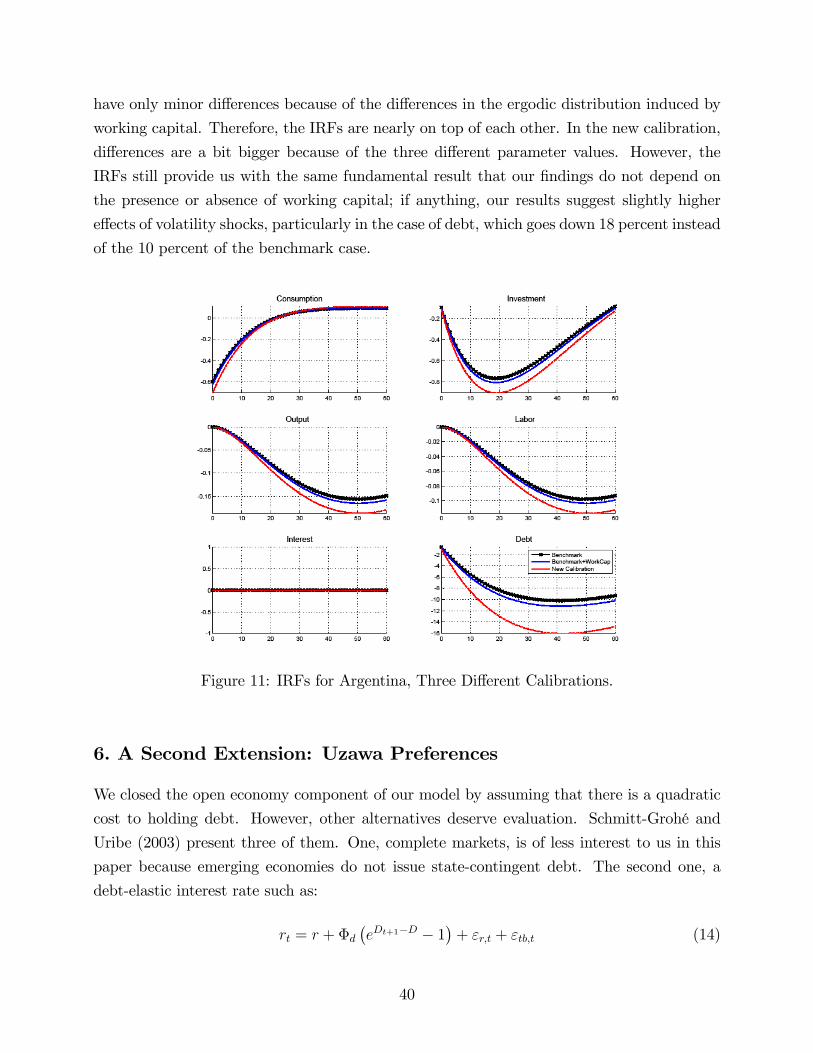
have only minor di¤erences because of the di¤erences in the ergodic distribution induced by

working capital. Therefore, the IRFs are nearly on top of each other. In the new calibration,

di¤erences are a bit bigger because of the three di¤erent parameter values. However, the

IRFs still provide us with the same fundamental result that our �ndings do not depend on

the presence or absence of working capital; if anything, our results suggest slightly higher

e¤ects of volatility shocks, particularly in the case of debt, which goes down 18 percent instead

of the 10 percent of the benchmark case.

Figure 11: IRFs for Argentina, Three Di¤erent Calibrations.

6. A Second Extension: Uzawa Preferences

We closed the open economy component of our model by assuming that there is a quadratic

cost to holding debt. However, other alternatives deserve evaluation. Schmitt-Grohé and

Uribe (2003) present three of them. One, complete markets, is of less interest to us in this

paper because emerging economies do not issue state-contingent debt. The second one, a

debt-elastic interest rate such as:

rt = r + �d�eDt+1�D � 1

�+ "r;t + "tb;t (14)

40

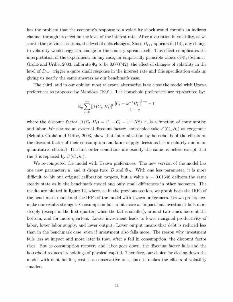
has the problem that the economy�s response to a volatility shock would contain an indirect

channel through its e¤ect on the level of the interest rate. After a variation in volatility, as we

saw in the previous sections, the level of debt changes. SinceDt+1 appears in (14), any change

to volatility would trigger a change in the country spread itself. This e¤ect complicates the

interpretation of the experiment. In any case, for empirically plausible values of �d (Schmitt-

Grohé and Uribe, 2003, calibrate �d to be 0.000742), the e¤ect of changes of volatility in the

level of Dt+1 trigger a quite small response in the interest rate and this speci�cation ends up

giving us nearly the same answers as our benchmark case.

The third, and in our opinion most relevant, alternative is to close the model with Uzawa

preferences as proposed by Mendoza (1991). The household preferences are represented by:

E01Xt=0

[� (Ct; Ht)]t [Ct � !�1H!

t ]1�v � 1

1� v

where the discount factor, � (Ct; Ht) = (1 + Ct � !�1H!t )��, is a function of consumption

and labor: We assume an external discount factor: households take � (Ct; Ht) as exogenous

(Schmitt-Grohé and Uribe, 2003, show that internalization by households of the e¤ects on

the discount factor of their consumption and labor supply decisions has absolutely minimum

quantitative e¤ects.) The �rst-order conditions are exactly the same as before except that

the � is replaced by � (Ct; ht).

We re-computed the model with Uzawa preferences. The new version of the model has

one new parameter, �, and it drops two: D and �D. With one less parameter, it is more

di¢ cult to hit our original calibration targets, but a value � = 0:01346 delivers the same

steady state as in the benchmark model and only small di¤erences in other moments. The

results are plotted in �gure 12, where, as in the previous section, we graph both the IRFs of

the benchmark model and the IRFs of the model with Uzawa preferences. Uzawa preferences

make our results stronger. Consumption falls a bit more at impact but investment falls more

steeply (except in the �rst quarter, when the fall is smaller), around two times more at the

bottom, and for more quarters. Lower investment leads to lower marginal productivity of

labor, lower labor supply, and lower output. Lower output means that debt is reduced less

than in the benchmark case, even if investment also falls more. The reason why investment

falls less at impact and more later is that, after a fall in consumption, the discount factor

rises. But as consumption recovers and labor goes down, the discount factor falls and the

household reduces its holdings of physical capital. Therefore, our choice for closing down the

model with debt holding cost is a conservative one, since it makes the e¤ects of volatility

smaller.

41

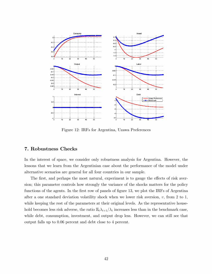
Figure 12: IRFs for Argentina, Uzawa Preferences

7. Robustness Checks

In the interest of space, we consider only robustness analysis for Argentina. However, the

lessons that we learn from the Argentinian case about the performance of the model under

alternative scenarios are general for all four countries in our sample.

The �rst, and perhaps the most natural, experiment is to gauge the e¤ects of risk aver-

sion; this parameter controls how strongly the variance of the shocks matters for the policy

functions of the agents. In the �rst row of panels of �gure 13, we plot the IRFs of Argentina

after a one standard deviation volatility shock when we lower risk aversion, v; from 2 to 1;

while keeping the rest of the parameters at their original levels. As the representative house-

hold becomes less risk adverse, the ratio Et�t+1=�t increases less than in the benchmark case,while debt, consumption, investment, and output drop less. However, we can still see that

output falls up to 0.06 percent and debt close to 4 percent.

42

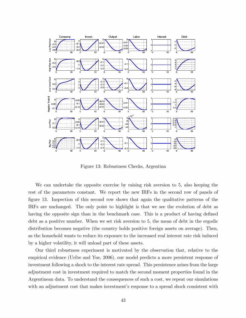
Figure 13: Robustness Checks, Argentina

We can undertake the opposite exercise by raising risk aversion to 5, also keeping the

rest of the parameters constant. We report the new IRFs in the second row of panels of

�gure 13. Inspection of this second row shows that again the qualitative patterns of the

IRFs are unchanged. The only point to highlight is that we see the evolution of debt as

having the opposite sign than in the benchmark case. This is a product of having de�ned

debt as a positive number. When we set risk aversion to 5, the mean of debt in the ergodic

distribution becomes negative (the country holds positive foreign assets on average). Then,

as the household wants to reduce its exposure to the increased real interest rate risk induced

by a higher volatility, it will unload part of these assets.

Our third robustness experiment is motivated by the observation that, relative to the

empirical evidence (Uribe and Yue, 2006), our model predicts a more persistent response of

investment following a shock to the interest rate spread. This persistence arises from the large

adjustment cost in investment required to match the second moment properties found in the

Argentinean data. To understand the consequences of such a cost, we repeat our simulations

with an adjustment cost that makes investment�s response to a spread shock consistent with

43

the evidence in Uribe and Yue. The results are reported in the third row of panels in �gure

13. We observe that 1) all variables but consumption become more responsive to a stochastic

volatility shock and 2) investment reaches its minimum in only one year after the shock. The

faster response of investment is a direct implication of the smaller adjustment costs.

The large contraction in economic activity when the adjustment cost is lower is explained

as follows. A smaller adjustment cost allows investment to easily drop after a volatility

shock. Such a drop has two e¤ects on households. First, it ameliorates the need to reduce

consumption in the aftermath of the shock and the household can use the additional proceeds

from lower investment to buy back debt. Second, capital will shrink tomorrow, thanks to a

smaller investment. Low capital in turn triggers low labor productivity, which reduces the

demand for labor and hence households�wealth. This decline in income ultimately exacer-

bates the contraction in future consumption. In the middle run, this second e¤ect dominates

the smaller reduction in consumption at impact, inducing a longer duration in its later drop.

We previously argued that a volatility shock to the interest rate is contractionary because

households consume less and save more in anticipation of possibly larger future interest rate

shocks. Then, an interesting question is what happens if the country has positive net assets,

Dt < 0. To answer this question, we repeat the experiment for the Argentinean calibration

M1, but we now assume that the economy starts with a net export-to-output ratio of -1.56

(the negative value of what we previously used). We report the results in the fourth row

of panels in �gure 13. Two features are worth mentioning: 1) a very mild recession follows

the volatility shock. Indeed, output and labor barely change. 2) Households de-accumulate

assets. The decline in assets results from risk-adverse households who fear that a negative

spread shock tomorrow may drive down the return of their foreign asset positions. The very

small declines in consumption and investment are caused by the household adjusting to a

possibly rather negative shock to their country spread in the next period that will reduce its

income from D.14

As a �nal robustness check, we discuss the implications of the priors on our model�s

predictions. To that end, we re-estimate the processes (2) and (4) for Argentina with two

alternative priors and report the results in table 13. For the �rst option (Case I), we select

relatively uninformative priors for �r and ��r centered in 0:5 while the other parameters�

priors remain the same as in the original exercise. For the same reason as in the original prior

(to minimize the impact of stochastic volatility), we endow �r with a tighter prior. Under

14This experiment begets the question of why the country is getting such a high rate of return on its foreignposition. A simple answer is that for every debtor paying a high interest rate, there is a creditor receiving ahigh interest rate. If we reduced the spread a country gets when Dt < 0, the results are qualitatively similarbut the IRFs are even smaller than those in the fourth row.

44

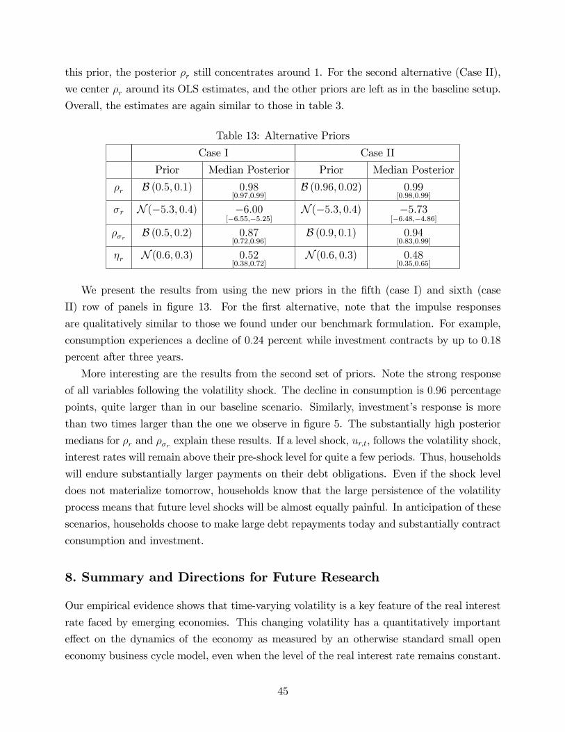
this prior, the posterior �r still concentrates around 1. For the second alternative (Case II),

we center �r around its OLS estimates, and the other priors are left as in the baseline setup.

Overall, the estimates are again similar to those in table 3.

Table 13: Alternative Priors

Case I Case II

Prior Median Posterior Prior Median Posterior

�r B (0:5; 0:1) 0:98[0:97;0:99]

B (0:96; 0:02) 0:99[0:98;0:99]

�r N (�5:3; 0:4) �6:00[�6:55;�5:25]

N (�5:3; 0:4) �5:73[�6:48;�4:86]

��r B (0:5; 0:2) 0:87[0:72;0:96]

B (0:9; 0:1) 0:94[0:83;0:99]

�r N (0:6; 0:3) 0:52[0:38;0:72]

N (0:6; 0:3) 0:48[0:35;0:65]

We present the results from using the new priors in the �fth (case I) and sixth (case

II) row of panels in �gure 13. For the �rst alternative, note that the impulse responses

are qualitatively similar to those we found under our benchmark formulation. For example,

consumption experiences a decline of 0:24 percent while investment contracts by up to 0.18

percent after three years.

More interesting are the results from the second set of priors. Note the strong response

of all variables following the volatility shock. The decline in consumption is 0:96 percentage

points, quite larger than in our baseline scenario. Similarly, investment�s response is more

than two times larger than the one we observe in �gure 5. The substantially high posterior

medians for �r and ��r explain these results. If a level shock, ur;t, follows the volatility shock,

interest rates will remain above their pre-shock level for quite a few periods. Thus, households

will endure substantially larger payments on their debt obligations. Even if the shock level

does not materialize tomorrow, households know that the large persistence of the volatility

process means that future level shocks will be almost equally painful. In anticipation of these

scenarios, households choose to make large debt repayments today and substantially contract

consumption and investment.

8. Summary and Directions for Future Research

Our empirical evidence shows that time-varying volatility is a key feature of the real interest

rate faced by emerging economies. This changing volatility has a quantitatively important

e¤ect on the dynamics of the economy as measured by an otherwise standard small open

economy business cycle model, even when the level of the real interest rate remains constant.

45

The mechanism behind the real e¤ects of volatility is that households with precautionary

behavior will change their holding of foreign debt as a response to changes in volatility to

reduce future �uctuations of marginal utility.

Our investigation opens the door to a set of interesting questions. First, and most obvi-

ously, why does volatility change over time? Is it related to some states of the economy? How

does it interact with other phenomena, such as debt default, debt renegotiation, or �nancial

market integration? Second, we would like to evaluate the possibilities of having time-varying

volatilities in other aspects of the economy. For example, in a recent and in�uential paper,

Aguiar and Gopinath (2007) have argued that one factor behind business cycle �uctuations in

emerging economies is recurrent changes in the productivity growth trend, possibly caused by

policy. It would be pro�table to explore the consequences of introducing stochastic volatility

in these changes.

46

9. Appendix

For completeness, this appendix includes the description of NIPA data used in section 2, a

brief introduction to the Particle �lter, a more detailed discussion of the consequences of

using a third-order approximation for the dynamics of the model, and the explanation of how

we compute the IRFs of the model.

9.1. NIPA Data

We obtain aggregate data from the International Financial Statistics (IFS) service of the

International Monetary Fund, except for Venezuela, for which data come from the Central

Bank of Venezuela (the IFS data set has some gaps for Venezuela). The data coverage

is: Argentina: 1993.Q1-2004.Q3; Brazil: 1995.Q1-2004.Q1; Ecuador: 1992.Q1-2001.Q2; and

Venezuela: 1991.Q1-2004.Q4. Consumption corresponds to household expenditure on goods

and services; investment is the sum of gross �xed capital formation and changes in inventories;

net exports equals exports of goods and services minus imports of goods and services; �nally,

output equals the addition of consumption, investment, and net exports. Real variables

were obtained by dividing nominal ones by the GDP de�ator. All variables were seasonally

adjusted using the U.S. Census Bureau�s X-12 program. Unless otherwise mentioned, output,

consumption, and investment are H-P �ltered.

9.2. Particle Filter

We present a brief introduction to the particle �lter. We will concentrate on the main idea

of the algorithm and skip most of the technical details. Doucet et al. (2001) is an excellent

reference of the interested reader. Fernández-Villaverde and Rubio-Ramírez (2007 and 2008)

are examples of applications in economics.

We want to evaluate the likelihood of the international risk-free real interest rate "tb;t and

the country spread deviations "r;t: Since the explanation of the �lter for the likelihood of one

process or the other is equivalent, we just take the �rst case.

The likelihood is costly to evaluate because of the non-linear interaction of volatility and

levels. Let us start by stacking all T observations of "tb;t in "Ttb and the parameters of the

process in : Given the Markov structure of our state space representation, we can factorize

the likelihood function as:

p�"Ttb;

�=

TYt=1

p�"tb;tj"t�1tb ;

�

47

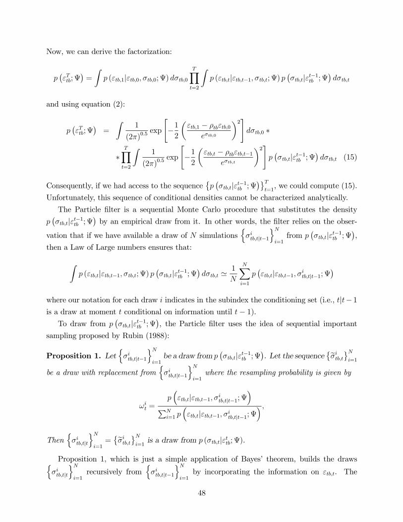
Now, we can derive the factorization:

p�"Ttb;

�=

Zp ("tb;1j"tb;0; �tb;0; ) d�tb;0

TYt=2

Zp ("tb;tj"tb;t�1; �tb;t; ) p

��tb;tj"t�1tb ;

�d�tb;t

and using equation (2):

p�"Ttb;

�=

Z1

(2�)0:5exp

"�12

�"tb;1 � �tb"tb;0

e�tb;0

�2#d�tb;0 �

�TYt=2

Z1

(2�)0:5exp

"�12

�"tb;t � �tb"tb;t�1

e�tb;t

�2#p��tb;tj"t�1tb ;

�d�tb;t (15)

Consequently, if we had access to the sequence�p��tb;tj"t�1tb ;

�Tt=1, we could compute (15).

Unfortunately, this sequence of conditional densities cannot be characterized analytically.

The Particle �lter is a sequential Monte Carlo procedure that substitutes the density

p��tb;tj"t�1tb ;

�by an empirical draw from it. In other words, the �lter relies on the obser-

vation that if we have available a draw of N simulationsn�itb;tjt�1

oNi=1

from p��tb;tj"t�1tb ;

�,

then a Law of Large numbers ensures that:

Zp ("tb;tj"tb;t�1; �tb;t; ) p

��tb;tj"t�1tb ;

�d�tb;t '

1

N

NXi=1

p�"tb;tj"tb;t�1; �itb;tjt�1;

�where our notation for each draw i indicates in the subindex the conditioning set (i.e., tjt� 1is a draw at moment t conditional on information until t� 1).To draw from p

��tb;tj"t�1tb ;

�, the Particle �lter uses the idea of sequential important

sampling proposed by Rubin (1988):

Proposition 1. Letn�itb;tjt�1

oNi=1be a draw from p

��tb;tj"t�1tb ;

�. Let the sequence

�e�itb;tNi=1be a draw with replacement from

n�itb;tjt�1

oNi=1

where the resampling probability is given by

!it =p�"tb;tj"tb;t�1; �itb;tjt�1;

�PN

i=1 p�"tb;tj"tb;t�1; �itb;tjt�1;

� ;Then

n�itb;tjt

oNi=1=�e�itb;tNi=1 is a draw from p (�tb;tj"ttb; ).

Proposition 1, which is just a simple application of Bayes� theorem, builds the drawsn�itb;tjt

oNi=1

recursively fromn�itb;tjt�1

oNi=1

by incorporating the information on "tb;t. The

48

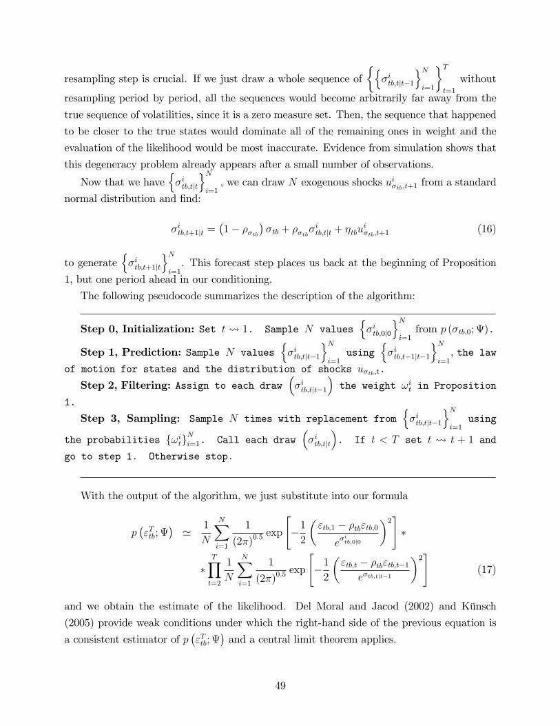
resampling step is crucial. If we just draw a whole sequence of�n

�itb;tjt�1

oNi=1

�Tt=1

without

resampling period by period, all the sequences would become arbitrarily far away from the

true sequence of volatilities, since it is a zero measure set. Then, the sequence that happened

to be closer to the true states would dominate all of the remaining ones in weight and the

evaluation of the likelihood would be most inaccurate. Evidence from simulation shows that

this degeneracy problem already appears after a small number of observations.

Now that we haven�itb;tjt

oNi=1

; we can draw N exogenous shocks ui�tb;t+1 from a standard

normal distribution and �nd:

�itb;t+1jt =�1� ��tb

��tb + ��tb�

itb;tjt + �tbu

i�tb;t+1

(16)

to generaten�itb;t+1jt

oNi=1. This forecast step places us back at the beginning of Proposition

1, but one period ahead in our conditioning.

The following pseudocode summarizes the description of the algorithm:

Step 0, Initialization: Set t 1. Sample N valuesn�itb;0j0

oNi=1

from p (�tb;0; ).

Step 1, Prediction: Sample N valuesn�itb;tjt�1

oNi=1

usingn�itb;t�1jt�1

oNi=1, the law

of motion for states and the distribution of shocks u�tb;t.

Step 2, Filtering: Assign to each draw��itb;tjt�1

�the weight !it in Proposition

1.

Step 3, Sampling: Sample N times with replacement fromn�itb;tjt�1

oNi=1

using

the probabilities f!itgNi=1. Call each draw

��itb;tjt

�. If t < T set t t + 1 and

go to step 1. Otherwise stop.

With the output of the algorithm, we just substitute into our formula

p�"Ttb;

�' 1

N

NXi=1

1

(2�)0:5exp

"�12

�"tb;1 � �tb"tb;0

e�itb;0j0

�2#�

�TYt=2

1

N

NXi=1

1

(2�)0:5exp

"�12

�"tb;t � �tb"tb;t�1

e�tb;tjt�1

�2#(17)

and we obtain the estimate of the likelihood. Del Moral and Jacod (2002) and Künsch

(2005) provide weak conditions under which the right-hand side of the previous equation is

a consistent estimator of p�"Ttb;

�and a central limit theorem applies.

49

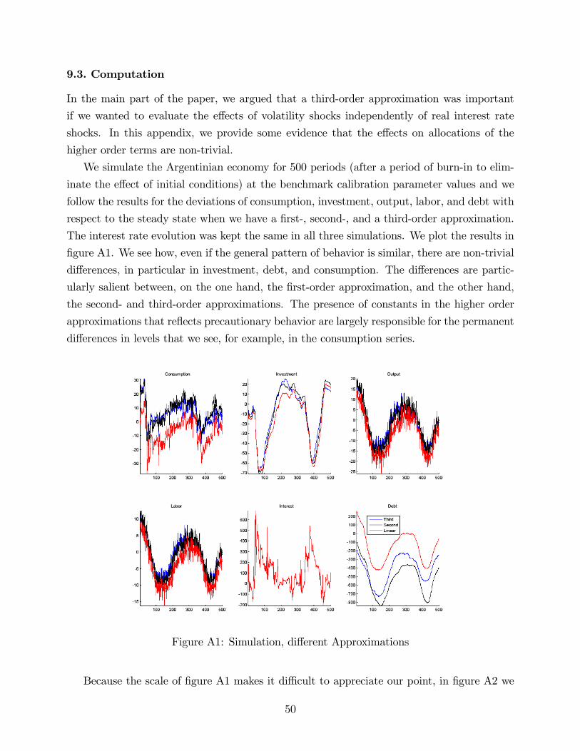
9.3. Computation

In the main part of the paper, we argued that a third-order approximation was important

if we wanted to evaluate the e¤ects of volatility shocks independently of real interest rate

shocks. In this appendix, we provide some evidence that the e¤ects on allocations of the

higher order terms are non-trivial.

We simulate the Argentinian economy for 500 periods (after a period of burn-in to elim-

inate the e¤ect of initial conditions) at the benchmark calibration parameter values and we

follow the results for the deviations of consumption, investment, output, labor, and debt with

respect to the steady state when we have a �rst-, second-, and a third-order approximation.

The interest rate evolution was kept the same in all three simulations. We plot the results in

�gure A1. We see how, even if the general pattern of behavior is similar, there are non-trivial

di¤erences, in particular in investment, debt, and consumption. The di¤erences are partic-

ularly salient between, on the one hand, the �rst-order approximation, and the other hand,

the second- and third-order approximations. The presence of constants in the higher order

approximations that re�ects precautionary behavior are largely responsible for the permanent

di¤erences in levels that we see, for example, in the consumption series.

Figure A1: Simulation, di¤erent Approximations

Because the scale of �gure A1 makes it di¢ cult to appreciate our point, in �gure A2 we

50

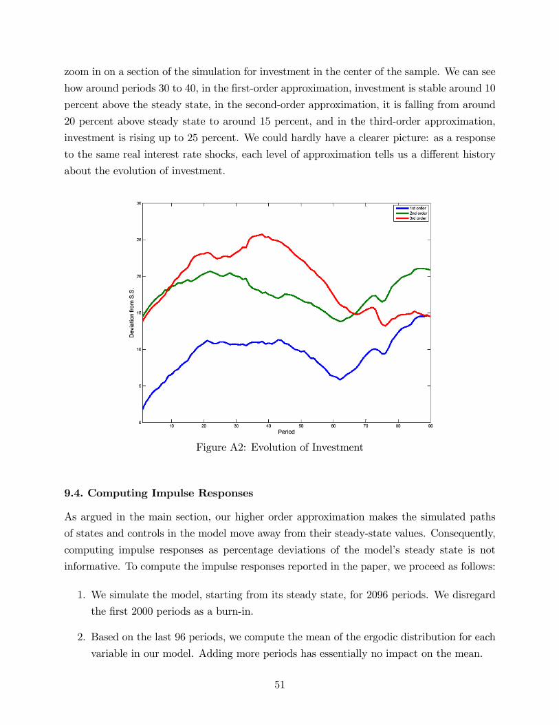
zoom in on a section of the simulation for investment in the center of the sample. We can see

how around periods 30 to 40, in the �rst-order approximation, investment is stable around 10

percent above the steady state, in the second-order approximation, it is falling from around

20 percent above steady state to around 15 percent, and in the third-order approximation,

investment is rising up to 25 percent. We could hardly have a clearer picture: as a response

to the same real interest rate shocks, each level of approximation tells us a di¤erent history

about the evolution of investment.

Figure A2: Evolution of Investment

9.4. Computing Impulse Responses

As argued in the main section, our higher order approximation makes the simulated paths

of states and controls in the model move away from their steady-state values. Consequently,

computing impulse responses as percentage deviations of the model�s steady state is not

informative. To compute the impulse responses reported in the paper, we proceed as follows:

1. We simulate the model, starting from its steady state, for 2096 periods. We disregard

the �rst 2000 periods as a burn-in.

2. Based on the last 96 periods, we compute the mean of the ergodic distribution for each

variable in our model. Adding more periods has essentially no impact on the mean.

51

3. Starting from the ergodic mean and in the absence of shocks, we hit the model with a

one standard deviation shock to the volatility process u�;t.

4. We report the resulting impulse responses as percentage deviations from the variables�

ergodic means.

In the context of a threshold model, Koop et al. (1996) have argued that the use of

the standard impulse response functions may be misleading. These authors urge the use

of the so-called generalized impulse response to overcome the drawbacks reported in their

manuscript. We computed the generalized impulse response, but we essentially found no

di¤erences between this procedure and the one outline above. We choose to report the

traditional impulse responses in the main body of the paper, since they are easier to interpret

than the generalized impulse response functions.

52

References

[1] Aguiar, M. and G. Gopinath (2007). �Emerging Market Business Cycle: The Cycle isthe Trend.�Journal of Political Economy 115, 1- 43.

[2] Alfaro, L., and F. Kanczuk (forthcoming). �Debt Maturity: Is Long-Term Debt Opti-mal?�Review of International Economics.

[3] Andersen, T. (1996). �Return Volatility and Trading Volume: An Information FlowInterpretation of Stochastic Volatility.�Journal of Finance 51, 69-204.

[4] Aruoba, B., J. Fernández-Villaverde, and J. Rubio-Ramírez (2006). �Comparing Solu-tion Methods for Dynamic Equilibrium Economies.�Journal of Economic Dynamic andControl 30, 2477-2508.

[5] Atkeson, A. and L.E. Ohanian (2001). �Are Phillips curves useful for forecasting in�a-tion?�Quarterly Review, Federal Reserve Bank of Minneapolis, 2-11.

[6] Bloom, N. (forthcoming). �The Impact of Uncertainty Shocks.�Econometrica.

[7] Broner, F., G. Lorenzoni, and S.L. Schmukler (2007). �Why Do Emerging EconomiesBorrow Short Term?�Mimeo.

[8] Campbell, J. Y. (2003). �Consumption-Based Asset Pricing.�In G.M. Constantinides,M. Harris, and R. M. Stulz (eds.), Handbook of the Economics of Finance 1, 803-887.North-Holland Elsevier.

[9] Correia I., J. Neves, and S. Rebelo (1995). �Business Cycles in Small Open Economies.�European Economic Review 39, 1089-1113.

[10] Del Moral P. and J. Jacod (2002), �The Monte-Carlo Method for Filtering with DiscreteTime Observations. Central Limit Theorems.�in T. J. Lyons and T. S. Salisbury (eds.),Numerical Methods and Stochastics. The Fields Institute Communications, AmericanMathematical Society.

[11] Doucet, A., N. de Freitas, and N. Gordon (2001). Sequential Monte Carlo Methods inPractice. Springer Verlag.

[12] Elder, J. (2004). �Another Perspective on the E¤ects of In�ation Uncertainty.�Journalof Money, Credit and Banking 36, 911-928.

[13] Fatás, A. (2002). �The E¤ects of Business Cycles on Growth.� in Norman Loayza andRaimundo Soto (eds), Economic Growth: Sources, Trends and Cycles. Central Bank ofChile.

[14] Fernández-Villaverde, J. and J. Rubio-Ramírez (2007). �Estimating MacroeconomicModels: A Likelihood Approach.�Review of Economic Studies 74, 1059-1087.

[15] Fernández-Villaverde, J. and J. Rubio-Ramírez (2008). �How Structural Are StructuralParameters?�NBER Macroeconomics Annual 2007, 83-137.

53

[16] Fountas, S. and M. Karanasos (2007). �In�ation, Output Growth, and Nominal andReal Uncertainty: Empirical Evidence for the G7.�Journal of International Money andFinance 26, 229-250.

[17] Grier, K.B. and M.J. Perry (2000). �The E¤ects of Real and Nominal Uncertainty onIn�ation and Output Growth: Some GARCH-M Evidence.�Journal of Applied Econo-metrics 15, 45-58.

[18] Guerrón-Quintan, P. (2009). �Do Uncertainty and Technology Drive Exchange Rates.�Mimeo, North Carolina State University.

[19] Hamilton, J. (2008). �Macroeconomics and ARCH.�Mimeo, University of California-SanDiego.

[20] Justiniano A. and G.E. Primiceri (2008). �The Time Varying Volatility of Macroeco-nomic Fluctuations.�American Economic Review 98, 604-641.

[21] Kaminsky, G.L., C.M. Reinhart and C.A. Vegh (2003). �The Unholy Trinity of FinancialContagion.�Journal of Economic Perspectives 17, 51-74.

[22] Kim, J., K. Sunghyun, E. Schaumburg, and C.A. Sims (2003). �Calculating and Us-ing Second Order Accurate Solutions of Discrete Time Dynamic Equilibrium Models.�Finance and Economics Discussion Series 2003-61, Board of Governors of the FederalReserve System.

[23] Koop G., M. Hashem Pesaran, and S. Potter (1996). �Impulse Response Analysis inNonlinear Multivariate Models.�Journal of Econometrics 74, 199-147.

[24] Künsch, H.R. (2005). �Recursive Monte Carlo Filters: Algorithms and TheoreticalAnalysis.�Annals of Statistics 33, 1983-2021.

[25] Kydland, F., and E. C. Prescott (1982). �Time to Build and Aggregate Fluctuations.�Econometrica 50, 1345�1370.

[26] Lee, K., S. Ni, and R. Ratti (1995). �Oil Shocks and the Macroeconomy: The Role ofPrice Variability.�Energy Journal 16, 39-56.

[27] Mendoza, E. (1991). �Real Business Cycles in a Small Open Economy.�American Eco-nomic Review 81, 797-818.

[28] Mendoza, E. (1995). �The Terms of Trade, the Real Exchange Rate, and EconomicFluctuations.�International Economic Review 36, 101-37.

[29] Neumeyer, P. and F. Perri (2005). �Business Cycles in Emerging Economies: the Roleof Interest Rates.�Journal of Monetary Economics 52, 345-380.

[30] Ramey, G. and V.A. Ramey (1995). �Cross-Country Evidence on the Link BetweenVolatility and Growth�American Economic Review 85, 1138-115.

54

[31] Roberts, G., A. Gelman, and W. Gilks (1997). �Weak Convergence and Optimal Scalingof Random Walk Metropolis Algorthims.�Annals of Applied Probability 7, 110-120.

[32] Ross, S. (1989). �Information and Volatility: The No-arbitrage Martingale Approach toTiming and Resolution Irrelevancy.�Journal of Finance 44, 1-17.

[33] Rubin, D.B. (1988). �Using the SIR Algorithm to Simulate Posterior Distributions�.in J.M. Bernardo, M.H. DeGroot, D.V. Lindley, and A.F.M. Smith (eds), BayesianStatistics 3, 395-402, Oxford University Press.

[34] Schmitt-Grohé S., and M. Uribe (2003). �Closing Small Open Economies.�Journal ofInternational Economics 61, 163-185.

[35] Shephard, N. (2008). �Stochastic Volatility.�The New Palgrave Dictionary of Economics.

[36] Stock, J.H. and M.W. Watson (2002). �Has the Business Cycle Changed, and Why?�NBER Macroeconomics Annual 17, 159-218.

[37] Stock, J.H. and M.W. Watson (2007). �Why Has U.S. In�ation Become Harder to Fore-cast?�Journal of Money, Credit and Banking 39, 3-33.

[38] Uribe M., and V. Yue (2006). �Country Spreads and Emerging Countries: Who DrivesWhom?�Journal of International Economics 69, 6-36.

55