RISK MANAGEMENT, INSURANCE AND SOCIAL NETWORKS IN GHANA

Jacqueline Vanderpuye-Orgle Ph.D. Candidate, Cornell University

Christopher B. Barrett

International Professor, Cornell University

Financial support for this research was provided by the United States Agency for International Development’s Strategies and Analyses for Growth and Access (SAGA) Project, the Social Science Research Council’s Program in Applied Economics on Risk and Development (through a grant from the John D. and Catherine T. MacArthur Foundation), the Yale Economic Growth Center and the Pew Charitable Trusts. We would like to thank the Institute of Statistical, Social and Economic Research (ISSER) at the University of Ghana, particularly Ernest Aryeetey, Ernest Appiah and Kudjoe Dovlo for providing an enabling research environment as well as invaluable support. We are also grateful to Christopher Udry, David Sahn, Ravi Kanbur, Donald Kenkel and participants at the SSRC Conference on Risk and Development (Santa Cruz, CA) for insightful comments. We are greatly indebted to Robert Ernest Afedoe, Raphael Arku, Setor Lotsu, Nana Owusu Kontoh and Sroda Lotsu for assistance with data collection. The views expressed here and remaining errors are the author’s and do not reflect any official agency. Copyright 2006 by Jacqueline Vanderpuye-Orgle and Christopher B. Barrett. All rights reserved. Readers may make verbatim copies of this document for non-commercial purposes by any means, provided that this copyright notice appears on all such copies.

1

1. Introduction For people in low-income, agrarian countries, risk management is crucial for their

very survival. In the ideal Arrow-Debreu world, complete markets with symmetric

information provide an array of contingent contracts and all decision-makers in the

economy can specify states of the world in which they make welfare improving

exchanges based on each other’s known preferences and beliefs. In this fictional

framework all risks can be addressed with market-based solutions.

In reality, the rural poor depend heavily on informal institutions for coping with

risk in the absence of well-developed insurance markets.1 The attendant intertemporal

consumption smoothing mechanisms are often available to only the relatively well-off

and well-placed subpopulations (Dercon 2002, De Weerdt 2005, Santos and Barrett

2006). Who is left out of these institutions? Allowing for the fact that these institutions

are based on endogenously formed networks as well as intrahousehold resource

allocation, is risk pooling Pareto efficient? To address these issues we draw on several

threads in the literature.

Social networks have been identified as loci of risk sharing. These networks are

fostered by kinship ties, ethnicity, geographical proximity, religion, and gender groups,

inter alia (Goldstein 1999, Santos and Barrett 2004, Udry and Conley 2004, De Weerdt

2005, Fafchamps and Gubert 2006, DeWeerdt and Dercon, 2006). However, some

marginal groups may be excluded from these networks. In particular, the poor may have

less dense risk sharing networks and may not have the wherewithal to make the nominal

contributions required by some of these mutual insurance groups or might also be

socially excluded (Dercon 2002, De Weerdt 2005, Dercon and DeWeerdt, 2006).

However, there is an even more ominous subpopulation who have not been given their

due in the development economics discourse – the socially invisible: those who are not

known in the community and are left out by default as against those who are known in

the community but excluded for a variety of reasons. 2

1 See Alderman and Paxson (1992), Besley (1995) and Bardhan and Udry (1999) for complete reviews. 2 Social distance is not symmetric. The characteristics of the socially excluded may not necessarily be the mirror-image or direct opposite of those include in these networks. In addition, the characteristics of the excluded may vary with the type of network link and nature of shock studied (Santos and Barrett 2004, Fafchamps and Gubert 2006, DeWeerdt and Dercon, 200).

2

Empirical tests often reject the provision of full insurance by social networks

(Deaton 1992, Townsend 1994, Gertler and Gruber 1997). Issues pertaining to

measurement error, asymmetric information and contract enforcement have been

identified as possible reasons (Alderman and Paxson 1992, Murgai et al. 2001). One

could argue that the hypothesis of full insurance will necessarily be rejected since these

tests are conducted for exogenously given groups such as the entire village, community,

clan as well as the household and hence may not adequately capture the true domain and

scope of risk sharing.3 In addition, most of these studies were undertaken at the

household level with the implicit assumption of a unitary household model: assuming

perfect substitutability among decision-makers as well as pooling of all resources within

the household. Yet there is ample evidence in the literature rejecting these assumptions.4

We hypothesize that if we correctly identify risk sharing networks, empirical tests

should yield complete insurance. In addition, if we correctly identify networks we can

also establish the characteristics of those who fall through the cracks--the subpopulation

without idiosyncratic risk insurance-- for the purposes of policy targeting. Thus our first

objective is to identify the socially invisible. The second objective is to test for risk

pooling within individuals’ networks. The point of departure of this paper from the extant

literature is thus twofold. Firstly, the analysis of social invisibility abstracts from the type

of network link examined and/ or shock experienced. Secondly, using a general

equilibrium framework, we test for full insurance within endogenously determined (self-

reported) networks at the individual-level.

The following section presents the data used in this study. Section 3 explores the

concept of social invisibility identifying the characteristics of the socially invisible in the

sample. Section 4 tests for risk pooling at the network level. Conclusions and policy

recommendations are presented in Section 5. The results showed the following: (i) Young

residents engaged in farming are more likely to be socially invisible, while belonging to a

major clan and having resided in the village for more than one generation reduces the

likelihood of being socially invisible. (ii) Risk pooling is complete for the socially

visible; we can reject the hypothesis that individual shocks affect individual consumption. 3 See Goldstein et al. (2005), Santos and Barrett (2006). 4 See Alderman, Chiappori, Haddad, Hoddinott and Kanbur (1995), Doss (1996), Udry (1996), Goldstein (1999), Duflo and Udry (2004).

3

In addition, individual consumption tracks village and network level average

consumption. On the other hand, risk pooling fails for the subsection of the population

that is socially invisible; we fail to reject both the full and partial insurance hypotheses at

the 5% level.

2. The Data The data used in this paper are from a rural household survey undertaken during

my dissertation field research from July 2004 to January 2005. This was the third wave of

a panel data set initiated by Christopher Udry and Markus Goldstein. The research was

conducted in the Akwapim South District (specifically, the Nsawam - Aburi area) in the

Eastern Region of Ghana. Since the early 1990s farmers in this area have been switching

from the cultivation of maize-cassava intercrop for domestic production to pineapple

cultivation for export. This transition involves a significant amount of risk by way of the

attendant new agronomic practices as well as exposure to global price fluctuations, hence

the need for insurance.5

The original sample was selected in 1996 using a two-stage procedure. Four

village clusters were purposively selected within this area based on their participation in

fruit and vegetable production as well as their array of agronomic, market access and

geographic conditions. Sixty married couples (or triples) were then randomly selected in

each village cluster, except for the smallest village cluster where all resident couples were

and interviewed individually. Male enumerators were assigned to male respondents and

female enumerators to female respondents to preserve gender sensitivity and cultural

norms. In all, 436 individuals were surveyed fifteen times in the first and second waves.

Of these, 372 individuals were surveyed three times in the third wave. The sample

attrition rate from the 1998-2004 interval was thus 14.68%. A brief description of the

modules relevant to the analyses in this paper is as follows.

5 See Goldstein and Udry (1999) for an in-depth discussion of the historical background of the area and the sampling techniques.

4

2.1 Individuals’ Social Networks

For each respondent, we randomly selected seven individuals in the sample from

the same village (without replacement).6 We then asked each respondent about their

knowledge of the match i.e., “Do you know__?”, followed a series of questions about

each match about their relationship with each of these matched individuals: how often

they talked with them, and whether or not he/she could approach the individual to deal

with one of a set of specific issues related to farming and credit. For example they were

asked, “Have you ever gone to (name) for advice on your farm?”

In administering the questionnaire we were sure to make the distinction between

knowing of someone (i.e., using the Akan translation of just “having heard of the

person”) and actually knowing the person. Knowing a random match in this sense is

indicative of an extant social link. This gives us a random sample of the individuals with

whom they have social links. By design, the characteristics of these random matches are

representative of people with whom they have extant social links, i.e., their social

networks. Even though we do not have the overall shape or size of the network, we know

about the type of people with whom they establish social links.

2.2 Consumption

We use data from detailed expenditure questionnaires to estimate consumption. Data

were collected on purchased food and general family expenses. Each respondent in the

household was asked if anyone in the household had purchased/ spent anything various

items for consumption in the past 12 months. If yes, we then asked them to disaggregate

the total value of the item and report the amount of money contributed by them, their

spouse and other members of the household, respectively, towards the purchase the item.

We used the modal frequencies of consumption from the previous rounds to determine

recall periods for the respective periods.

Even though these expenditure questionnaires were administered at the individual

level with the head, and spouse(s) of head being interviewed separately regarding

contributions made towards purchasing an item, actual individual consumption levels of

6 Respondents were also non-randomly matched with three other village-specific “focal” individuals identified from the community-studies approach taken in a preliminary field trip as individuals in the villages from whom advice is commonly sought. We focus on the random matches in this study.

5

the respective items were not assigned. Hence, we follow Goldstein (1999) in assigning

the following items that are typically purchased for own-consumption to the respective

respondent’s private consumption: alcoholic beverages, non-alcoholic pre-packaged

beverages, prepared food (from kiosks), personal care products, hair cuts, public

transport, petrol, care repairs, newspapers, entertainment, lottery tickets and kola nuts.

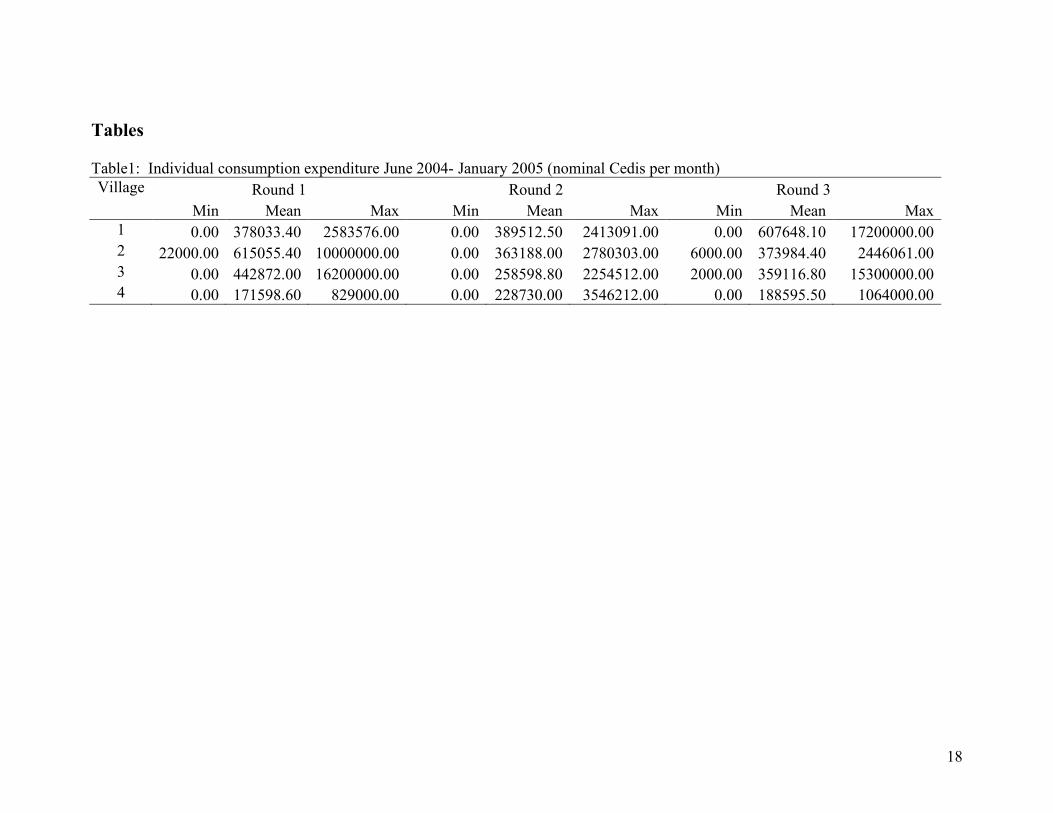
Summary statistics on the total individual expenditure on these goods per village and

round are presented in Table 1.

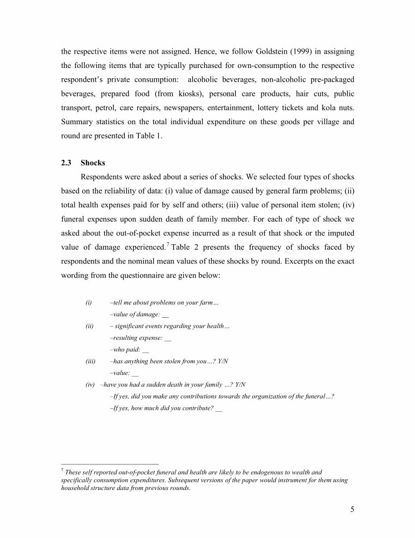
2.3 Shocks

Respondents were asked about a series of shocks. We selected four types of shocks

based on the reliability of data: (i) value of damage caused by general farm problems; (ii)

total health expenses paid for by self and others; (iii) value of personal item stolen; (iv)

funeral expenses upon sudden death of family member. For each of type of shock we

asked about the out-of-pocket expense incurred as a result of that shock or the imputed

value of damage experienced.7 Table 2 presents the frequency of shocks faced by

respondents and the nominal mean values of these shocks by round. Excerpts on the exact

wording from the questionnaire are given below:

(i) –tell me about problems on your farm…

–value of damage: __

(ii) – significant events regarding your health…

–resulting expense: __

–who paid: __

(iii) –has anything been stolen from you…? Y/N

–value: __

(iv) –have you had a sudden death in your family …? Y/N

–If yes, did you make any contributions towards the organization of the funeral…?

–If yes, how much did you contribute? __

7 These self reported out-of-pocket funeral and health are likely to be endogenous to wealth and specifically consumption expenditures. Subsequent versions of the paper would instrument for them using household structure data from previous rounds.

6

2.4 Other Sample Characteristics

The household roster, assets and family background questionnaires provide

detailed descriptions of sample characteristics used in the subsequent analysis. Table 3

presents the summary statistics on the individual characteristics for the entire sample.

3. Social Invisibility

Clifford (1963) explicitly defined social visibility “as the position an individual

occupies within a group as it is perceived by other members of the group. This position is

achieved through the competencies (skills and attributes) or lack of them, that the

individual possesses which are relevant to the ongoing process of the group.” By

extension, he defined social invisibility as when “the individual occupies space within the

group but is perceived by others as contributing little other than his own presence.” We

deviate from this a bit, defining social invisibility as when the individual occupies space

within a group, in this case residing in the village or community, but is not recognized or

known by other members of that group. We define a continuum of social visibility. Let N

be the number of times the respondent’s name was drawn in the random matching

process; n be the number of times the respondent is known by others when presented as a

random match. The latter allows for asymmetry in network structures. We then estimate

the level of social visibility, SV, as follows:

10 , !!= SVN

nSV (1)

We then discretize this continuum of social invisibility, classifying an individual as

Socially Invisible if SV=0. A person is Known if SV>0. The descriptive statistics on N, n

and SV are presented in Table 3. Each individual was presented on average 5 times as a

random match, out of which they were known on average by 3 respondents. 26 of the

respondents (i.e. 8.39%) were socially invisible. We tested among alternative thresholds

for defining invisibility and this proved optimal.

Table 4 presents summary statistics on the individual characteristics for the

Known and the Socially Invisible. Structural differences between the characteristics of

the Known and Socially Invisible matches were assessed by a two-sided t-test for equal

7

means. Five key facts emerge from this table. First, the socially invisible are

predominantly female (only 23% of them are male). Second, they are younger than their

Known counterparts. Third, an overwhelming majority (90%) have been fostered-- living

in the care of persons other than their parents and outside of their homes for at least a year

while growing up. Fourth, more of them were the first generation to reside in the village

and finally fewer of them had parents who have held village offices.

These cross-tabulations are reinforced by a multivariate analysis. Let itl =1 be an

indicator variable that individual i is socially invisible at time t. Let Pr{itl =1} be the

probability that itl =1 conditional on some individual characteristics,

itX . We then

estimate:

Pr{itl =1}= )0( >+!

ititX "# (2)

By probit regression, where ! is the normal CDF. We estimate a random effects model

clustering the observations on the respondent’s identity. The probit estimates of the

likelihood that an individual is socially invisible are presented in Table 5.

The results show that the older are less likely to be socially invisible. In addition,

having an occupation other than farming reduces the likelihood of being invisible. This is

consistent with Santos and Barrett’s (2004) results using these same data but a different

model: teachers and traders are more likely to be known and the older are less likely to

know the younger members of community. Belonging to a major clan reduces the

likelihood of being invisible since one may establish links with members of ones’

matrikin (Goldstein 1999, De Weerdt 2002, Santos and Barrett 2004, Udry and Conley

2004). Having resided in the village for more than one generation reduces the likelihood

of becoming invisible. This may be attributed to the fact that relationships established in

the community are invariably built upon by progeny. On the other hand, having education

beyond the middle school level increases the likelihood of being socially invisible. This is

counterintuitive: one might expect the relatively highly educated to be widely known in

the community.8 However, De Weerdt (2002) found that “households with educated

members tend to lie closer to each other on the network graph.” By assortative matching,

8 See Basu and Foster (1998) for related discussions.

8

the relatively highly educated are more likely to be linked to each other and since they

have fewer cohorts (i.e., they make up only 7.03% of the population) they appear less

likely to be known by others. In addition, the relatively highly educated may have left the

village for a number of years in pursuit of education.

Being male, having been fostered, and having parents who held village offices

were consistent with the cross tabulations in sign but not statistically significant even at

the 10% level. Males are less likely to be socially invisible. Similarly, respondents whose

parents held village offices are less likely to be invisible. However, having been fostered

increases the likelihood of being socially invisible.9

This definition of social invisibility relies on the knowledge of a subset of the

sample (i.e. ranging from 1 to 15 people) to whom the respondent’s name was presented

as a random match. To extend this subset to the entire village, a probit model was

estimated to determine the likelihood of being known when presented as a random match

using the algebraic distance between social links and allowing for symmetry (Santos and

Barrett, 2004). The results are presented in Table 7. Respondents who were both male,

had the same level of education, had resided in the village for more than one generation

and belonged to the same clan were more likely to know each other. Older, poorer

respondents who were farmers or traders were more likely to be known. In addition,

females were more likely to know males, males were more likely to know females and

non-farmers were more likely to know farmers. On the other hand, farmers were less

likely to know non-farmers, respondents who were fostered were less likely to know

those who were not fostered and less likely to know each other.

Out-of-sample predictions were made to determine the likelihood of being known

by members of the entire village. Categorical variables were then generated using 0.1

point intervals of the predicted probability of being known, i.e. Known=1 if the predicted

probability ≥ x and 0 otherwise, where x = 0.1, 0.2,…, 0.9. A SV continuum was

calculated for each of these variables using the number of times the respondent is known

by others in the village as the numerator and the village size minus one as the

denominator. Different cut-offs of the SV continuum were then used to define the Socially 9 The results are robust to different cut-offs of the SV continuum. Table 6 shows that defining Socially Invisible=1 if SV=0, 0.05, 0.10, 0.15, 0.20, 0.25, 0.30, 0.35 and 0.40 respectively, with Socially Invisible=0 otherwise, as well using the continuous SV yield qualitatively identical results.

9

Invisible. In particular, Socially Invisible=1 if SV≥0, 0.05, 0.10, 0.15, 0.20, 0.25, 0.30,

0.35 and 0.40 respectively, 0 otherwise were generated and used in the subsequent

analyses as a robustness check. Socially Invisible=1 if SV<0.25 and 0 otherwise, for

Known=1 if Predicted Probability ≥ 0.8, maximized the log likelihood. By this definition

22.79% of the sample was socially invisible.

4. Risk Pooling

Shocks are pervasive in most agrarian societies, the study area being no exception.

We use data on (i) the value of damage caused by general farm problems, (ii) total health

expenses paid for by self and others, (iii) value of personal item stolen, and (iv)

contributions made towards organization of funeral upon sudden death of family member

to represent shocks in this study. For each of type of shock we asked about the out-of-

pocket expense incurred as a result of that shock or the imputed value of damage

experienced if no direct expenses were incurred.

Over all three rounds, 56% of the respondents reported having suffered health

problems, 51% had suffered a sudden death in the family, death and funerals pose a huge

financial burden on family in this area. 32% of the respondents suffered a variety of farm

problems, the most prevalent being infestation by grasscutters (a common rodent in the

area). Only 15% of the respondents experienced theft of a personal item. Only one

respondent mentioned erratic rainfall as a problem. Covariate events such as rainfall

patterns were not the primary concern in these essentially farming communities.

Shocks are also very costly. Health expenditures were the most important in

magnitude. Respondents spent, on average, 531613Cedis on health shocks and lost

221743Cedis to farm problems, 218186Cedis to funeral expenses and 80658Cedis on

theft.10

To what extent are these shocks insured? Is risk fully pooled at the village level or

at the network level? Are the socially invisible insured? To address these questions, we

use a model akin to that of Townsend (1994).

10 The mean exchange rate over the reference period was 9000Cedis/ $1.00.

10

Suppose there are S possible states of the world, each occurring with objective,

constant and commonly known probability πs. Assume individuals have preferences that

are additive across time and over states of nature and common rates of time preference βt,

where λin is the programming weight associated with individual i in network n. Suppose

there are K networks in the economy with N members in each network.11 Let cinst and yinst

be individual i in network n’s consumption and income in state s at time t, respectively,

then we can denote the Pareto efficient allocation of risk by the following problem:

( )!"

#$%

&' ''= ==

inst

T

t

S

s

st

N

i

inCcU

inst

0 11

max ()* (3)

subject to:

!!==

=N

i

inst

N

i

inst yc11

(4)

The first order condition is given by:

( ) ( )jnstjninstin cUcU '' !! = (5)

Suppose each individual’s preferences can be represented by an exponential utility

function:

( ) [ ]instinstccU !

!"#$

%&'

("= exp1 (6)

Substituting (6) into (5), taking logs and rearranging terms, we get

!"

#$%

&'=

in

jn

jnstinstcc

(

(log (7)

which on aggregating across all individuals in a network gives

!"

#$%

&++= ''

==

N

j

jnin

N

j

jnstinstN

cN

c11

log1

log11

(()

(8)

11 For now, we abstract from the fact that networks may be interlinked: an individual may belong to more than one network. We’ll explore this possibility later in examining the extent to which risk is spread among networks.

11

Let !"

#$%

&+=' (

=

N

j

jninN 1

log1

log1

))*

(9)

Then (9) implies that

nnstinst

cc !+= (10)

where nstc is the network mean consumption excluding i and En is a constant that allows

for dispersion in consumption levels among network members. But this dispersion is

fixed over time and states of nature. Equation (10) reveals that contemporaneous own

income, yinst, is irrelevant to the determination of individual consumption. As in Goldstein

(1999) we decompose contemporaneous own income for i in network n into a permanent

component iny and an idiosyncratic component

instx . The latter represents an i.i.d shock

of mean zero, representing the transitory shocks experienced by individuals in the

sample. Own income is thus:

instininstxyy += (11)

Including (11) in (10), we can test for full insurance using contemporaneous own income

as an exclusion restriction:

( )nnstinstininst

cxyc !+++= "#$ (12)

Taking the first difference yields:

instnstnstinstinstinstinstccxxcc !"# +$+$=$ $$$ )()( 111 (13)

where inst! is an i.i.d error term. A testable full risk pooling hypothesis is then H0: β =0,

γ=1 versus HA: β >0, γ<1. An analogous testable full risk pooling hypothesis was derived

for the individual i in village j by substituting cijst and yijst for consumption and income

respectively in equations (3) and (4). Similarly, a hypothesis for network k in village j

may be derived by substituting ckjst and ykjst for consumption and income respectively in

equations (3) and (4).

We estimated equation (13) and conducted F-tests for the joint hypothesis of full risk

pooling. We also test for partial risk pooling at the village and network level, respectively

12

using H0: β =0 versus HA: β >0. We use agricultural, health, theft and mortality shocks as

proxies forinstx .

We assess the extent to which any individual (visible or invisible) pools risk with

other individuals in the village. We regress the change in individual private consumption

expenditures on the change in farm, health, theft and mortality shocks as well as the

change in residual village average consumption (i.e., excluding person i). Table 8 shows

that individual private consumption is fairly smooth and tracks village average

consumption directly, albeit not one-for-one. A unit change in the village average

consumption corresponds to a 0.47 change in individual private consumption. The

positive effect implies that individual consumption varies in response to covariate shocks

that affect in village average consumption implying that household expenditures are

affected by shocks to others, implying some social insurance. In addition, the various

idiosyncratic shocks do not have a significant effect on individual consumption even at

the 10% significance level. Individual consumption does not seem to vary in response to

the experience of own shocks. While an F-test rejects the null hypothesis of full

insurance, it fails to reject the partial insurance hypothesis, even at the 10% level. Even

though individuals are insured, full risk pooling is not achieved at the village level.

We now disaggregate the data into socially visible and socially invisible

individuals. We then regress the change in private consumption expenditures of visible

individuals on the change in their farm, health, theft and mortality shocks as well as the

change in residual village average consumption (i.e. excluding person i) for the other

visible individuals in the village. The change in average consumption of visible

individuals within the village has a stronger, positive and more statistically significant

effect on private consumption for visible individuals, as compared to the pooled results

for the entire village. The various shocks again have no significant effect on individual

private consumption even at the 10% level. Their estimated magnitudes are smaller than

in the pooled regression. We fail to reject the hypotheses that the mean value of the

change in loss due to farm problems, change in total health expenses, change in theft of

personal item and change in expenses due to sudden death, respectively, are not

significantly different from zero. Most notably, an F-test fails to reject both the full and

partial insurance hypotheses even at the 20% level. Visible individuals appear to achieve

13

something at least very close to full risk pooling with other visible individuals in the

village.12

We now focus on the socially invisible, assessing the extent to which an invisible

individual pools risk with all other individuals in the village. We regress the change in

private consumption expenditures of invisible individuals on the change in their farm,

health, theft and mortality shocks as well as the change in residual village average

consumption for the entire village (i.e., excluding person i). The F-tests reject both the

full and partial insurance hypotheses at the 5% level.13 The change in village average

consumption has a much smaller, positive, albeit still statistically significant, effect on

private consumption for invisible individuals as compared to visible individuals in the

village. A unit change in the village average consumption corresponds to a 0.25 unit

change in individual consumption. However, individual consumption responds strongly

to the shocks the individual experiences. All the shocks have a statistically significant

effect on consumption at the 1% level. Plainly, socially invisible individuals’

consumption varies strongly in response to the shocks they suffer while socially visible

individuals’ consumption does not.

By order of magnitude, health and mortality shocks have the least effect on

consumption followed by thefts and farm shocks. Individual consumption changes by

17%, 38%, 88% and 106% with unit changes in health, mortality, theft and farm shocks,

respectively. This difference in the effects of the respective shocks may be attributed to a

number of factors. For instance, tradition places more value on life than inanimate objects

hence a theft, although considered unfortunate, is not viewed as crucial to survival and

hence may not garner the same level of support as a health shock. Moreover, custom

requires that one would call on the sick and the bereaved.14 The latter enforces some

12 We also tested for full risk pooling of visible individuals with all other individuals in the entire village. The results showed that visible individuals only partially pool risk with the entire village comprising of both the socially visible and invisible. This is to be expected since by definition the visible do not have any social connections with the socially invisible in the village. 13 We replicate the analysis to test for full risk pooling by the invisible with other invisible individuals in the village. The results are similar. The F-tests reject both the full and partial insurance hypotheses at the 5% level. 14 It is customary for a sick person to send a message to friends and family informing them about his/her predicament. In addition, one has to go and “greet” the bereaved and offer them drinks and/ or cash towards the organization of the funeral. In the Akan tradition the latter is termed “wo ko bo nsawa” (translated as “going to give a donation towards the funeral”).

14

generalized reciprocity with regards to health and mortality shocks. Second, whereas a

health shock is readily observable/ verifiable, thefts and farm shocks, other than extreme

cases may not be obvious to all others in the village. People do not assist with shocks

they do not know happened.

The directions of change as per the signs on the coefficients of shocks are mixed.

Whereas theft of personal items and expenses due to a sudden death in the family have

the expected negative sign, losses due to farm problems and health expenses have a

positive effect on individual private consumption.

To this point, we have explored risk pooling at the village. Now, conditional on

being visible, we assess the extent to which an individual pools risk with members of his/

her network. We use the mean individual consumption for the known random matches as

a proxy for network average consumption. 15 We regress the change in private

consumption of visible individuals on the change in farm, health, theft and mortality

shocks as well as the change in this residual network average consumption (i.e.,

excluding person i). The results in Table 9 are similar to that of visible individuals in a

village. Individual consumption comoves with network average consumption. In this case

the change in village average consumption is not statistically significant. The respective

shocks do not have a significant effect on individual private consumption even at the 10%

level. We fail to reject the hypotheses that the mean value of the change farm losses,

health expenses, theft and mortality shocks, respectively, are not significantly different

from zero. The F-test fails to reject both the full and partial insurance hypotheses even at

the 10% level. Visible individuals achieve full risk pooling with other individuals in their

networks.

Finally, we assess the extent to which these respective networks pool risk with

other networks in the village. Given interlinkages, networks may serve to re-insure each

other. Taking the network as a unit, we regress the change in network average

consumption expenditures on the change in network-level mean farm, health, theft and

mortality shocks as well as the change in residual average consumption for all networks

in the village (i.e. excluding network i). The results are given in Table 10. Network

15 Subsequent versions of this paper will predict known individuals in the sample from the random matches and use their mean individual consumption as a proxy for network average consumption.

15

average consumption statistically significantly comoves almost one-for-one with village

average consumption. With the exception of health expenses, we fail to reject the

hypotheses that the mean value of the change in loss due to farm problems, change in

theft of personal item and change in expenses due to sudden death, respectively, are not

significantly different from zero. Nonetheless, the F-test rejects both full and partial risk

pooling hypotheses even at the 10% level. This may be due to the fact that we limited the

data to intra-village networks. Networks may cross village lines. In fact, it may be these

‘weak ties’ that serve the very purpose of spreading risk, e.g., social re-insurance.

The results show that individual private consumption is fairly smooth for all

individuals in the village, particularly the visible. However, full risk pooling is not

achieved at the exogenously given village level. Unpacking this result by disaggregating

the data shows that full risk pooling is achieved by visible individuals with other visible

individuals both at the village and at the network levels. On the other hand, the socially

invisible fail to achieve either full or partial risk pooling at the village level (and amongst

themselves) and the latter pool risk at both the network and the village levels.16

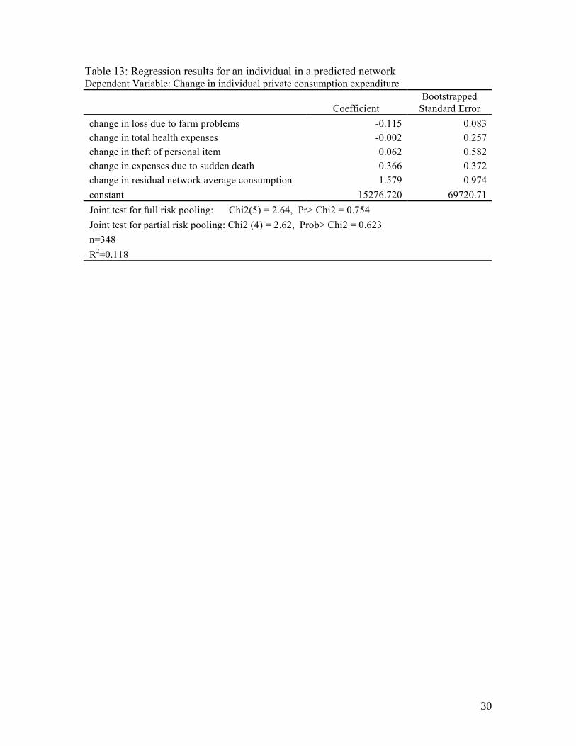
Tables 12-14 replicate the analyses using Social Invisibility derived from the

predicted probability of being known by all individuals in the village. The regression

coefficients estimated using bootstrapped standard errors also illustrates that individuals

fail to achieve full risk pooling at the exogenously given village level. Visible individuals

attain full risk pooling with other individuals within the village and within their networks.

However, using this extended construct, the socially invisible achieve partial risk pooling

with individuals within the village and networks reinsure each other, yielding partial risk

pooling of networks by other networks within the village.

16 Table 10 presents a summary of the F-tests. We also re-estimated the regressions using different thresholds of the SV continuum -- defining Socially Invisible=1 if SV=0, 0.05, 0.10, 0.15, 0.20, 0.25, 0.30, 0.35 and 0.40 respectively, with Socially Invisible=0 otherwise in order to endogenously determine the ‘break point’ in the continuum. The estimated model diagnostics show that the definition used in the paper (i.e. Socially Invisible=1 if SV=0) yields the best fit. This result is supported by pooling the data, estimating a fully interacted model and testing for equality of coefficients at the respective cut-offs of the SV continuum. Results are available upon request.

16

5. Conclusions Although risk management is crucial for survival, it may be very costly and

simply unavailable to some subpopulations. This paper identified the characteristics of

the socially excluded on the basis of the concept of social invisibility, abstracting from

the type of network link examined and/or shock experienced. Using a general equilibrium

framework, we assessed full insurance within endogenously determined networks.

Finally, focusing on credit we examined the state-contingent nature of credit contracts at

the individual level.

The results showed that younger residents who are in the farming occupation are

more likely to be socially invisible. In addition, not belonging to a major clan and having

resided in the village for only one generation increases the likelihood of being socially

invisible. By extension, migrants are more likely to be socially invisible.

With regards to risk pooling, individual private consumption is fairly smooth for

all individuals in the village, particularly the visible. However, full risk pooling is not

achieved at the exogenously given village level. Unpacking this result by disaggregating

the data, the analysis shows that full risk pooling is achieved by visible individuals with

other visible individuals both at the village and at the network levels. We can reject the

hypotheses that individual private consumption responds to respective adverse shocks. In

addition, individual consumption commoves with village and network level average

consumption levels. On the other hand, risk pooling seems to fail for the subsection of the

population that is socially invisible; we fail to reject both the full and partial insurance

hypotheses at the 5% level. The socially invisible fail to achieve either full or partial risk

pooling at the village level (and amongst themselves).

Using the construct of Social Invisibility derived from the predicted probability of

being known by entire village, individuals fail to achieve full risk pooling at the

exogenously given village level. Visible individuals attain full risk pooling with other

individuals within the village and within their networks. However, the socially invisible

achieve partial risk pooling with individuals within the village and networks reinsure

each other to some extent, yielding partial risk pooling with networks within the village.

17

In summary, the study shows that individuals insure within networks, in fact risk

pooling is perfect at this level. In addition networks are distinct from villages thus

assuming that the entire village is an exogenously given network results in less than

perfect risk pooling. There are people who are excluded from these networks who are left

relatively uninsured. What we need to know is who is connected and who is not

connected, paying particular attention to the latter subpopulation.

By way of policy implications, the first best solution to the issue of risk is a set of

interventions designed to improve access to and the functioning of formal rural financial

institutions and to establish insurance facilities. However, in the face of information

asymmetry, contract enforcement and incentive problems we propose that the second best

solution, based on the results of this paper, would be to first to invest in developing the

potential for social networks to insure members against risk by, for instance, extending

access to credit through social network akin to microcredit for those with extant social

links, allowing for the for pure consumption loans given nonseparability adherent with

risk.

Evidence of Pareto efficient allocation of idiosyncratic risk among members of

social networks suggests that given binding financial constraints, policy should

distinguish between idiosyncratic versus covariate risk: policy targeting for idiosyncratic

shocks should focus on those left out of these networks (i.e. the socially invisible)

whereas interventions ex poste of covariate shocks should target everyone, both members

of social networks and the socially invisible for whom we now have identifying

characteristics. Given the evidence that the socially invisible are farmers we also propose

the use of contract interlinkages as a means of quasi- insurance: interlinking credit and

product sales or input delivery (using the output as implicit collateral in areas where land

tenure systems do not allow for outright seizure) to provide alternate means of insuring

this subpopulation. The proposed interventions would help improve agricultural

productivity and ultimately enhance the welfare of the agrarian poor.

18

Tables Table1: Individual consumption expenditure June 2004- January 2005 (nominal Cedis per month) Village Round 1 Round 2 Round 3

Min Mean Max Min Mean Max Min Mean Max 1 0.00 378033.40 2583576.00 0.00 389512.50 2413091.00 0.00 607648.10 17200000.00 2 22000.00 615055.40 10000000.00 0.00 363188.00 2780303.00 6000.00 373984.40 2446061.00 3 0.00 442872.00 16200000.00 0.00 258598.80 2254512.00 2000.00 359116.80 15300000.00 4 0.00 171598.60 829000.00 0.00 228730.00 3546212.00 0.00 188595.50 1064000.00

19

Table 2: Percentage of individuals affected by shocks and mean actual expenditure/ imputed value of damage(nominal Cedis) Shocks Round 1 Round 3 Round 3 Frequency Mean value Frequency Mean value Frequency Mean value Farm problems 52.0 534517.20 22.8 69518.38 20.6 41157.51 Total Health Expenses 72.2 1219493.00 50.0 189789.70 46.0 141478.00 Theft of personal item 19.1 145696.60 13.7 51944.85 11.0 40175.82 Sudden death 50.5 440430.80 55.9 96011.03 45.6 103827.80

20

Table 3: Summary statistics on random matching Variable Mean Median Min Max Number of times presented as a match (N) 5.00 5.00 1 15 Number of times known as a match (n) 3.38 3.00 0 13 Social Visibility (SV) 0.67 0.75 0 1

21

Table 4: Descriptive statistics of variables Frequency (%) Variable Definition

Entire Sample

Known Socially Invisible

Male =1 if male, 0 otherwise 47.56 49.45 22.86* Age Respondent’s age 45.51

(12.95) 45.87

(13.12) 40.76* (9.38)

Level of Schooling No schooling Primary School Middle School Higher School

=1 if respondent has no schooling, 0 otherwise =1 if primary level, 0 otherwise =1 if middle school or junior secondary school, 0 otherwise =1 if any higher, 0 otherwise

25.15 17.01 50.81 7.03

25.11 16.56 51.21 7.13

25.71 22.86 45.71 5.72

Occupation Farmer Other Unemployed

=1 if farmer, 0 otherwise =1 if trader, artisan, teacher, civil servant, office or health worker, agricultural or non- agricultural labor, 0 otherwise =1 if student/ pupil, unemployed or not in the labor force

78.92 18.64

2.44

78.84 18.86

2.30

80.00 15.71

4.29

Number of matches known

Number of random matches known 4.48 (2.08)

4.54 (2.06)

3.55* (2.22)

Major clan =1 if member of a major clan, 0 otherwise 88.05 88.68 78.43 Herelong =1 if not the first generation to reside in

village 74.36 75.80 51.92*

Parents held office =1 if parents holds any village office, 0 otherwise

47.07 48.06 31.37*

Fostered =1 if respondent was fostered, 0 otherwise 78.19 77.37 90.48* Value of non-land assets

Value of all farm and business equipment in; money held in bank, susu, esusu, bonds, pension, foreign currency and cash on hand; jewelry; cloth; and animals millions of Cedis

499.98 (9381.44)

202.84 (1399.56)

481.62 (9093.30)

Value of inheritance

Total value of any current and expected land and non-land inheritance in millions of Cedis

11144.81 (182120.90)

11859.00 (187862.80)

23.80 (65.85)

Location Village 1 Village 2 Village 3 Village 4

=1 if Village cluster 1, 0 otherwise =1 if Village cluster 2, 0 otherwise =1 if Village cluster 3, 0 otherwise =1 if Village cluster 4, 0 otherwise

25.76 22.91 24.34 26.99

26.64 24.34 21.82 27.19

14.29* 4.29*

57.14* 24.29

Note: The characteristics with significant differences in means at the 5% level are indicated with an asterisk. The standard deviations of continuous variables are given in parentheses.

22

Table 5: Probit estimation of Social Invisibility Variables Coefficient Prob>|z|

Dependent Variable: Socially invisible Individual Characteristics Male -0.291 0.338 Age -0.031** 0.016 Middle school education -- --

No schooling -0.334 0.260 Primary school education 0.261 0.299 Higher than middle school 0.758*** 0.100 Farmer -- -- Other occupation -0.730*** 0.065 Unemployed -0.197 0.768 Assets Value of nonland wealth 0.001 0.803 Value of inheritance -0.032 0.737 Social characteristics Major clan -0.533** 0.049 Herelong -0.598* 0.008 Fostered 0.070 0.849 Parents held office -0.081 0.718 Location Village 2 -0.614 0.132 Village 3 1.117* 0.000 Village 4 0.461 0.118 n = 572 Log likelihood = -100.33 Wald chi2(16) = 55.31 Prob>chi2 = 0.000

* Significant at the 1% level ** Significant at the 5% level *** Significant at the 10% level

23

Table 6: Robustness tests of Social Invisibility Correlates

Social Visibility Index Cut-off SV = 0, 0.05, 0.10 SV = 0.15 SV = 0.20 SV = 0.25 SV = 0.30 SV = 0.35 SV = 0.40 SV continuum Variables Coeff. Prob>|z| Coeff. Prob>|z| Coeff. Prob>|z| Coeff. Prob>|z| Coeff. Prob>|z| Coeff. Prob>|z| Coeff. Prob>|z| Coeff. Prob>|z| Individual Characteristics Male -0.29 0.34 -0.22 0.46 -0.17 0.59 -0.18 0.57 -0.22 0.46 -0.34 0.20 -0.51*** 0.06 -0.09** 0.02 Age -0.03** 0.02 -0.01 0.35 -0.01 0.39 -0.01 0.50 -0.01 0.33 -0.02*** 0.07 -0.02*** 0.07 0.00*** 0.07 Middle school education No schooling -0.33 0.26 -0.10 0.75 -0.14 0.67 -0.08 0.82 0.01 0.99 0.05 0.85 -0.01 0.98 0.00 0.95 Primary school education 0.26 0.30 0.29 0.31 0.30 0.33 0.27 0.40 0.27 0.36 -0.03 0.92 0.08 0.76 0.01 0.86 Higher than middle school 0.76*** 0.10 0.61 0.19 0.20 0.70 0.14 0.79 0.11 0.84 -0.10 0.83 0.00 0.99 0.00 0.94 Farmer Other occupation -0.73*** 0.07 -0.49 0.18 -0.31 0.39 -0.39 0.29 -0.51 0.14 -0.25 0.37 -0.35 0.20 -0.06*** 0.09 Unemployed -0.20 0.77 -0.03 0.97 -0.14 0.86 -0.21 0.81 -0.24 0.77 -0.78 0.36 -0.98 0.27 0.01 0.94 Assets Value of nonland wealth 0.00 0.80 0.00 0.97 0.00 0.97 0.00 0.96 0.00 0.93 0.00 0.87 0.00 0.78 0.00 0.56 Value of inheritance -0.03 0.74 -0.04 0.73 -0.04 0.75 -0.03 0.75 -0.01 0.83 -0.01 0.83 -0.01 0.73 0.00 0.88 Social characteristics Major clan -0.53** 0.05 -0.53*** 0.09 -0.42 0.25 -0.56 0.13 -0.31 0.37 -0.37 0.25 -0.32 0.35 -0.10** 0.05 Herelong -0.60* 0.01 -0.50** 0.04 -0.44 0.12 -0.56** 0.05 -0.83* 0.00 -0.68* 0.01 -0.60** 0.02 -0.10* 0.01 Fostered 0.07 0.85 0.45 0.25 0.17 0.65 0.28 0.47 0.30 0.42 0.14 0.65 0.07 0.83 0.00 1.00 Parents’ held office -0.08 0.72 -0.24 0.30 -0.30 0.24 -0.24 0.36 -0.16 0.52 -0.27 0.21 -0.25 0.26 -0.04 0.24 Location Village 2 -0.61 0.13 -0.75*** 0.10 -0.64 0.12 -0.44 0.26 -0.61 0.11 -0.40 0.20 -0.49 0.12 -0.11* 0.01 Village 3 1.12* 0.00 1.17* 0.00 1.38* 0.00 1.55* 0.00 1.29* 0.00 1.14* 0.00 1.16* 0.00 0.23* 0.00 Village 4 0.46 0.12 0.47 0.13 0.38 0.24 0.36 0.29 0.38 0.22 0.49 0.08 0.65** 0.02 0.05 0.21 * Significant at the 1% level ** Significant at the 5% level *** Significant at the 10% level

24

Table 7: Probit estimation of the likelihood of knowing a random match

* Significant at the 1% level ** Significant at the 5% level *** Significant at the 10% level

Variables Coefficient Prob>|z| Both male 1.030* 0.000 Female, male 0.394* 0.000 Male, female 0.200** 0.029 Older 0.152** 0.024 Same education 0.213* 0.000 Same occupation -0.119 0.230 Trader, non-trader -0.375 0.131 Non-trader, trader 0.207 0.121 Farmer, non-farmer -0.527* 0.000 Non-farmer, farmer 0.542* 0.000 Same clan 0.245* 0.001 Both herelong 0.327* 0.001 Herelong, not-herelong 0.012 0.913 Not-herelong, herelong 0.061 0.562 Both fostered -0.291** 0.004 Fostered, not-fostered -0.317** 0.004 Not-fostered, fostered 0.032 0.762 Poorer 0.111** 0.054 Age 0.003 0.323 Value of nonland wealth 0.000 0.433 Farmer 0.723* 0.000 Trader 0.776** 0.003 Village 2 0.187*** 0.094 Village 3 -0.754* 0.000 Village 4 -0.199*** 0.055 n=3724 Log likelihood = -1952.09 Wald chi2(25) = 342.66 Prob>chi2 = 0.000

25

Table 8: Regression results for respective groups individuals in a village Dependent Variable: Change in individual private consumption expenditure All Individuals Visible Individuals Invisible Individuals Coefficient Standard Error Coefficient Standard Error Coefficient Standard Error change in loss due to farm problems -0.063 0.049 0.010 0.024 1.058* 0.122 change in total health expenses 0.001 0.001 0.001 0.001 0.172* 0.012 change in theft of personal item 0.023 0.037 -0.010 0.017 -0.877* 0.078 change in expenses due to sudden death 0.002 0.008 0.002 0.008 -0.377* 0.059 change in residual village average consumption 0.469*** 0.242 0.641* 0.294 0.248* 0.127 constant -14267.170 59931.500 -7214.325 66886.680 142473.100* 0.122 Joint test for full risk pooling F(5, 239) = 0.73, Prob>F= 0.02 F(5, 202) = 1.36, Prob>F= 0.24 F(5, 12) =294.11, Prob>F= 0.00 Joint test for partial risk pooling F(4, 239) = 0.81, Prob>F= 0.61 F(4, 202) = 0.50, Prob>F= 0.74 F(4, 12) =190.69, Prob>F= 0.00 n=514 n=460 n=70 R2=0.011 R2=0.009 R2=0.949

* Significant at the 1% level ** Significant at the 5% level *** Significant at the 10% level

26

Table 9: Regression results for an individual in a network Dependent Variable: Change in individual private consumption expenditure Coefficient Standard Error change in loss due to farm problems 0.003 0.020 change in total health expenses 0.001 0.001 change in theft of personal item -0.011 0.018 change in expenses due to sudden death 0.001 0.008 change in residual network average consumption 0.353 0.344 constant -6615.284 66595.230 Joint test for full risk pooling: F(5, 202) = 0.77, Prob>F = 0.57 Joint test for partial risk pooling: F(4, 202) = 0.17, Prob>F = 0.95 n=460 R2=0.026

27

Table 10: Regression results for insurance among networks in a village Dependent Variable: Change in network average consumption expenditure Coefficient Standard Error change in loss due to farm problems -0.001 0.016 change in total health expenses 0.002 0.000 change in theft of personal item -0.034 0.100 change in expenses due to sudden death 0.005 0.005 change in residual village average consumption 1.020 0.286 constant -6125.933 44128.900 Joint test for full risk pooling: F(5, 177) = 23.68, Prob>F = 0.00 Joint test for partial risk pooling: F(4, 177) = 11.34, Prob>F = 0.00 n=434 R2=0.063

28

Table 11: Summary of results for tests for risk pooling Full Risk Pooling Partial Risk Pooling An individual in a village Rejected Not rejected A visible individual in a village Not rejected Not rejected An invisible individual in a village Rejected Rejected An individual in a network Not rejected Not rejected A network in a village Rejected Rejected

29

Table 12: Regression results for respective groups individuals in a village using predicted probability of knowing match, with bootstrapped standard errors Dependent Variable: Change in individual private consumption expenditure All Individuals Visible Individuals Invisible Individuals Coefficient Standard Error Coefficient Standard Error Coefficient Standard Error change in loss due to farm problems -0.070 0.049 -0.069 0.062 -0.021 0.125 change in total health expenses 0.001 0.252 -0.003 0.673 -0.027 0.123 change in theft of personal item 0.016 0.228 0.028 0.523 -0.542 0.451 change in expenses due to sudden death 0.006 0.155 0.430 0.508 -0.004 0.174 change in residual village average consumption 0.247 0.208 0.369 0.317 0.163 0.206 constant -11460.91 77871.73 40075.17 104281.50 2348.58 127943.10 Joint test for full risk pooling Chi2(5) = 18.68, Pr> Chi2= 0.002 Chi2(5) = 6.56, Pr> Chi2= 0.255 Chi2 (5) =2.01, Pr> Chi2= 0.734

Joint test for partial risk pooling Chi2 (4) = 2.20, Pr> Chi2 = 0.700 Chi2 (4) = 3.12, Pr> Chi2= 0.538 Chi2 (4) =54.71, Pr> Chi2= 0.000

n=469 n=351 n=118 R2=0.014 R2=0.042 R2=0.069

30

Table 13: Regression results for an individual in a predicted network Dependent Variable: Change in individual private consumption expenditure

Coefficient Bootstrapped

Standard Error change in loss due to farm problems -0.115 0.083 change in total health expenses -0.002 0.257 change in theft of personal item 0.062 0.582 change in expenses due to sudden death 0.366 0.372 change in residual network average consumption 1.579 0.974 constant 15276.720 69720.71 Joint test for full risk pooling: Chi2(5) = 2.64, Pr> Chi2 = 0.754 Joint test for partial risk pooling: Chi2 (4) = 2.62, Prob> Chi2 = 0.623 n=348 R2=0.118

31

Table 14: Regression results for insurance among predicted networks in a village Dependent Variable: Change in network average consumption expenditure

Coefficient Bootstrapped

Standard Error change in loss due to farm problems -0.077 0.058 change in total health expenses -0.003 0.595 change in theft of personal item 0.041 0.377 change in expenses due to sudden death 0.433 0.399 change in residual village average consumption 0.068 0.058 constant -315361.60 252212.40 Joint test for full risk pooling: Chi2(5) = 280.24, Pr> Chi2 = 0.000 Joint test for partial risk pooling: Chi2 (4) = 3.35, Prob> Chi2 = 0.501 n=351 R2=0.063

32

References Alderman, H., and Paxson, C. H. (1992). Do the Poor Insure? A Synthesis of the

Literature on Risk and Consumption in Developing Countries. Washington DC, The World Bank.

Alderman, H., Chiappori, P.A., Haddad, L., Hoddinott, J., and Kanbur, R. (1995). Unitary

Versus Collective Models of the Household: Is it Time to Shift the Burden of Proof? World Bank Research Observer. 10: 1-9.

Anderson, J. E. (1949). The Psychology of Development and Personal Adjustment. Texas,

Holt, Rinehart and Winston. Arnott, R., and Stiglitz, J.E. (1991). Moral Hazard and Nonmarket Institutions:

Dysfunctional Crowding Out or Peer Monitoring? American Economic Review. 81(1): 179-90.

Bardhan, P., and Udry C. (1999). "Risk and Insurance in an Agricultural Economy," in

Development Economics. Oxford: Oxford University Press, 94-109. Barrett, C. (2004). Smallholder Identities and Social Networks: The Challenge of

Improving Productivity and Welfare. In C. Barrett (Ed.), The Social Economics of Poverty: Identities Groups, Communities and Networks. London: Routeledge.

Barrett, C. (2005a). The Social Economics of Poverty. London: Routeledge. Barrett, C. (2005b). Displaced Distortions: Financial Market Failures and Seemingly

Inefficient Resource Allocation. Ithaca, New York, Cornell University. Basu, K. and Foster J. (1998). "On Measuring Literacy." Economic Journal 108(451):

1733-49. Bell, C., Srinivasan T. N., and Udry C. (1997). Rationing, Spillover, and Interlinking in

Credit Markets: The Case of Rural Punjab. Oxford Economic Papers, 49, 557-585.

Besley, T. (1995a). Nonmarket Institutions for Credit and Risk Sharing in Low Income

Countries. Journal of Economic Perspectives. 9(3): 115-127. Besley, T (1995a). Savings, Credit and Insurance. In J. Behrman, and T. N. Srinivasan

(Eds.), Handbook of Development Economics. 2123-2207. Amsterdam; New York and Oxford: Elsevier Science North Holland.

Besley, T., and Coate, S. (1995). Group Lending, Repayment Incentives and Social

Collateral. Journal of Development Economics. 46(1): 1-18. Clifford, E. (1963). "Social Visibility." Child Development 34(3): 799-808.

33

De Weerdt, J. (2005). Risk-Sharing and Endogenous Network Formation. In S. Dercon (Ed.), Insurance Against Poverty. 197-216. New York: Oxford University Press.

De Weerdt, J and Dercon, S. (2006). Risk-Sharing Networks And Insurance Against

Illness. Journal of Development Economics, 81,337–356. Deaton, A. (1992). Savings and Income Smoothing in Cote D'ivoire. Journal of African

Economies, 1, 1-24. Dercon, S. (2005). Risk, Poverty and Public Action. In S. Dercon (Ed.), Insurance

Against Poverty. 439-450. New York: Oxford University Press. Dock, T., Marot, E., Platteau, J.P., and Sail, A. (1993). Commercialization, Credit et

Assurance dans la Peche Artisanale: Le cas du Senegal. Madras: Samudra Publicatons.

Doss, C. R. (1996). Intrahousehold Resource Allocation in an Uncertain Environment.

American Journal of Agricultural Economics, 78, 1335-1339. Duflo, E., and Udry, C. (2004). Intrahousehold Resource Allocation in Cote d'Ivoire:

Social Norms, Separate Accounts and Consumption Choices. Gertler, P., and Gruber J. (1997). Insuring Consumption against Illness. National Bureau

of Economic Research Working Paper Series. 6035:1-57. Goldstein, M. (1999). Chop Time, No Friends: Intrahousehold and Individual Insurance

Mechanisms in Southern Ghana. Mimeo. Goldstein, M., De Janvry, A., and Sadoulet, E. (2005). Is a Friend in Need a Friend

Indeed? Inclusion and Exclusion in Mutual Insurance Networks in Southern Ghana. In S. Dercon (Ed.), Insurance Against Poverty. New York: Oxford University Press.

Fafchamps , M. and Gubert, F. (2006) The Formation of Risk Sharing Networks. Journal

of Development Economics. Forthcoming. Hauge, S. (2002). Household, Group and Program Factors in Group-Based Agricultural

Credit Delinquency. Mimeo. La Ferrara, E. (2003). Kin Groups and Reciprocity: A Model of Credit Transactions in

Ghana. American Economic Review. 93(5): 1730-1751. Ligon, E., Thomas, J.P., and Worrall, T. (2002). Informal Insurance Arrangements with

Limited Commitment: Theory and Evidence from Village Economies. Review of Economic Studies. 69(1): 209-44.

34

Lybbert, T.J., Barrett, C.B., Desta, S., and Coppock, D.L. (2004). Stochastic Wealth Dynamics and Risk Management Among a Poor Population. The Economic Journal. 114: 750–777.

Murgai, R., Winters, P., Sadoulet E., and De Janvry A. (2001). "Localized and

Incomplete Mutual Insurance," Journal of Development Economics, 67, 245-274. Santos, P., and Barrett, C. (2004). Interest and Identity in Network Formation: Who do

Smallholders Seek out for Information in Rural Ghana?: Cornell University. Santos, P., and Barrett, C. (2006). Informal Insurance in the Presence of Poverty Traps:

Evidence from Ethiopia: Cornell University. Stiglitz, J.E. (1990). Peer Monitoring and Credit Markets. World Bank Economic Review.

4(3): 351-66. Thomas, J.P., and Worrall, T. (1994). Informal Insurance Arrangements in Village

Economies. Townsend, R. (1982). Optimal Multiperiod Contracts and the gain from Enduring

Relationships under Private Information. Journal of Political Economy. 90(6): 116-86.

Udry, C. (1996). Gender, Agricultural Production and the Theory of the Household.

Journal of Political Economy. 104 (5): 1010-1046. Udry, C., and Conley, T. (2005). Social Networks in Ghana. In C. Barrett (Ed.), The

Social Economics of Poverty. London: Routeledge. Varian, H. 1990. Monitoring Agents with Other Agents. Journal of Institutional and

Theoretical Economics. 146: 153-74.