Risk Management and Governance Interest rate risk management

Prof. Hugues Pirotte

Introduction Interest rate risk (IR risk) is more difficult to manage

» Various interest rates in each currency, not perfectly correlated

» We need a function describing the variation of the rate with maturity, the term structure of interest rates or yield curve.

» The points of the curve do not show only parallel movements.

Tools available » Duration and convexity measures (equivalent to delta-gamma in previous

slides)

» Partial durations

» Multiple deltas

» Principal component analysis

» Evolution around the latter like ICA

2 Prof. H. Pirotte

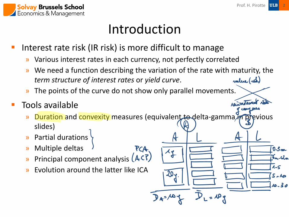
Zero-rates n-year zero-coupon interest rate =

» Interest earned on an investment starting today and lasting n years.

» n-year spot rate, n-year zero rate, n-year zero

» Annual compounded and continuous compounded rates:

The term structure of zero-rates is also called the zero-curve.

0, and 0,cr t r t

3 Prof. H. Pirotte

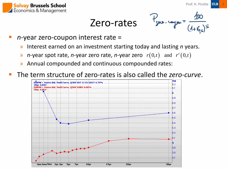
Forward rates Annual compounded version

Continuously compounded version

Practitioners use also the previous approach when they work with intra-annual forwards

1 2 1 2

1 1 2 21 0, 1 , 1 0,t t t t

r t f t t r t

2 12

1

2

1 2

1

1 0,, 1

1 0,

t tt

t

r tf t t

r t

1 1 1 2 2 1 2 20, , 0,r t t f t t t t r t t

2 2 1 1

1 2

2 1

0, 0,,

r t t r t tf t t

t t

4 Prof. H. Pirotte

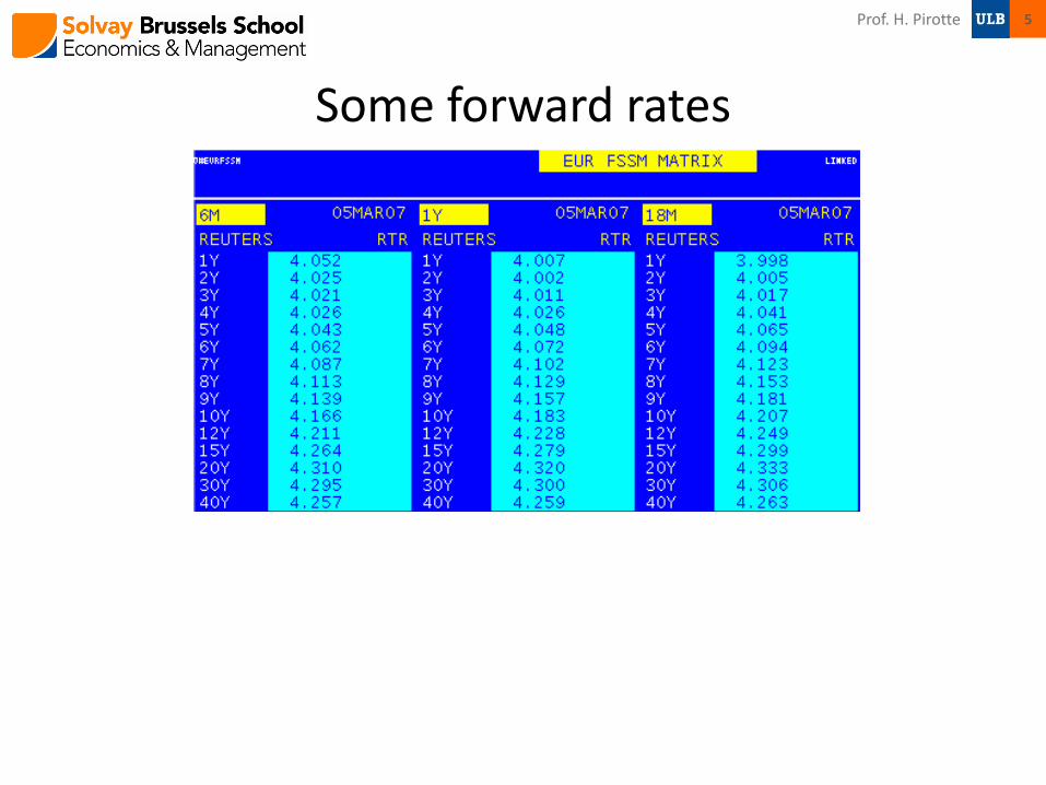
Some forward rates

5 Prof. H. Pirotte

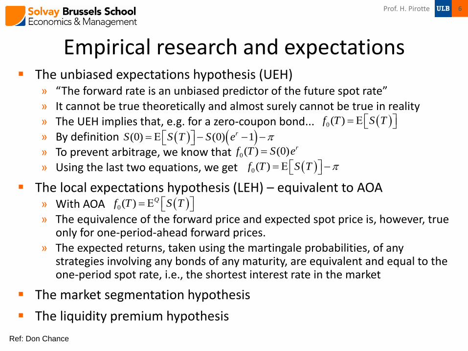
Empirical research and expectations The unbiased expectations hypothesis (UEH)

» “The forward rate is an unbiased predictor of the future spot rate” » It cannot be true theoretically and almost surely cannot be true in reality » The UEH implies that, e.g. for a zero-coupon bond... » By definition » To prevent arbitrage, we know that » Using the last two equations, we get

The local expectations hypothesis (LEH) – equivalent to AOA » With AOA » The equivalence of the forward price and expected spot price is, however, true

only for one-period-ahead forward prices. » The expected returns, taken using the martingale probabilities, of any

strategies involving any bonds of any maturity, are equivalent and equal to the one-period spot rate, i.e., the shortest interest rate in the market

The market segmentation hypothesis

The liquidity premium hypothesis

0( )f T S T

(0) (0) 1rS S T S e

0( ) (0) rf T S e

0( )f T S T

0( ) Qf T S T

Ref: Don Chance

6 Prof. H. Pirotte

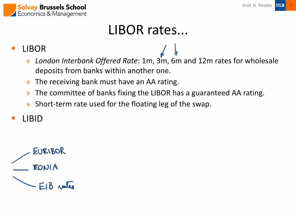
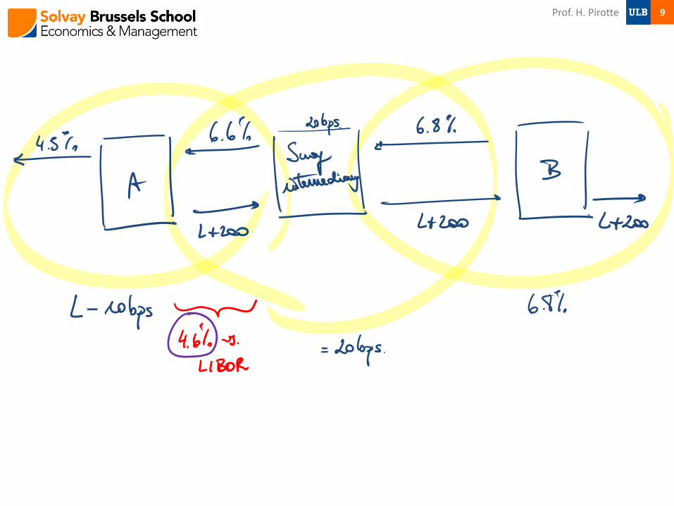
LIBOR rates... LIBOR

» London Interbank Offered Rate: 1m, 3m, 6m and 12m rates for wholesale deposits from banks within another one.

» The receiving bank must have an AA rating.

» The committee of banks fixing the LIBOR has a guaranteed AA rating.

» Short-term rate used for the floating leg of the swap.

LIBID

7 Prof. H. Pirotte

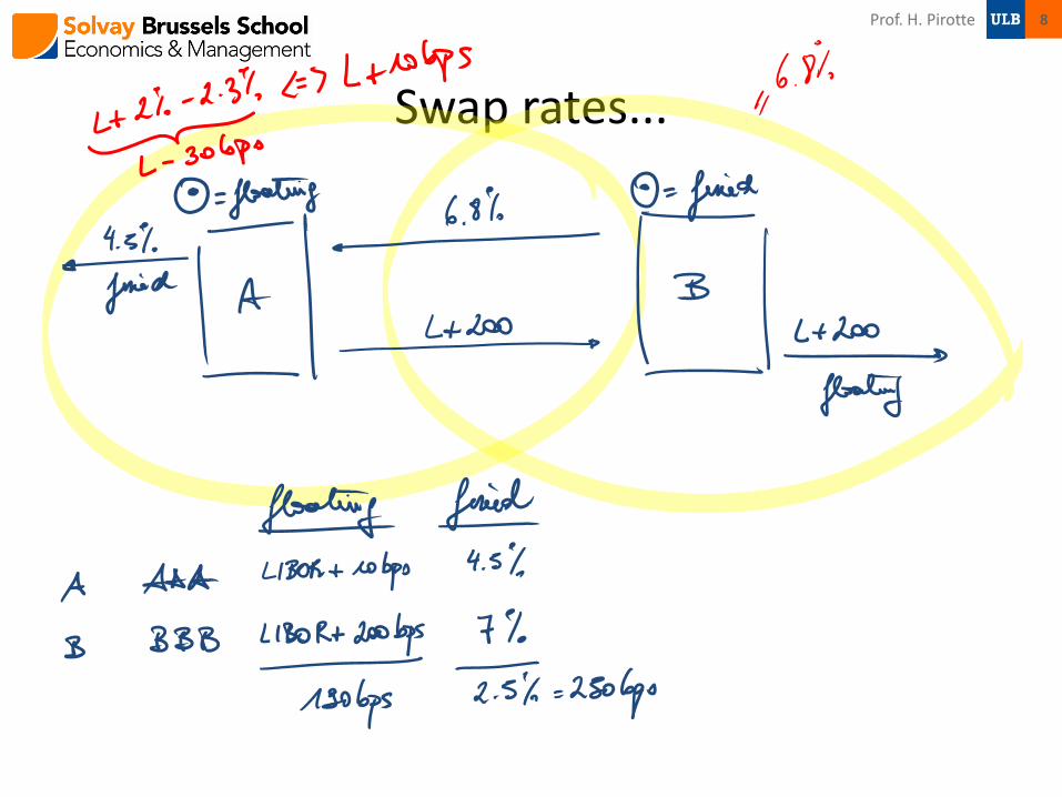
Swap rates...

Prof. H. Pirotte 8

9 Prof. H. Pirotte

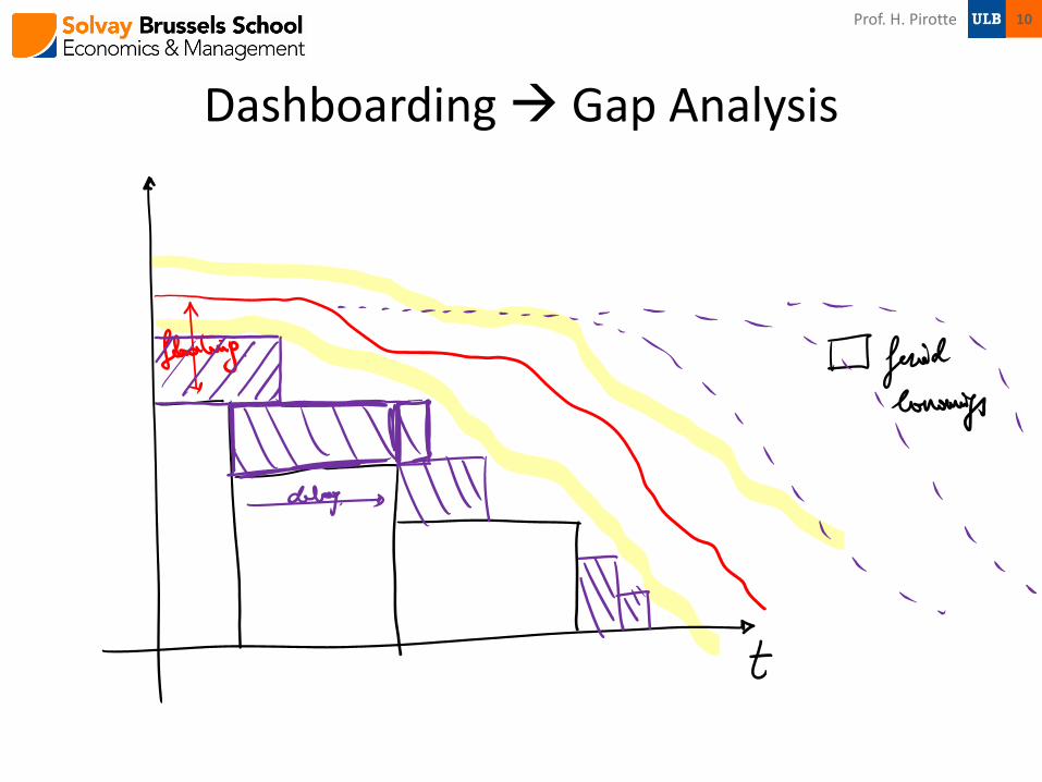
Dashboarding Gap Analysis

Prof. H. Pirotte 10

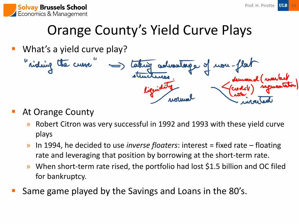
Orange County’s Yield Curve Plays What’s a yield curve play?

At Orange County » Robert Citron was very successful in 1992 and 1993 with these yield curve

plays

» In 1994, he decided to use inverse floaters: interest = fixed rate – floating rate and leveraging that position by borrowing at the short-term rate.

» When short-term rate rised, the portfolio had lost $1.5 billion and OC filed for bankruptcy.

Same game played by the Savings and Loans in the 80’s.

11 Prof. H. Pirotte

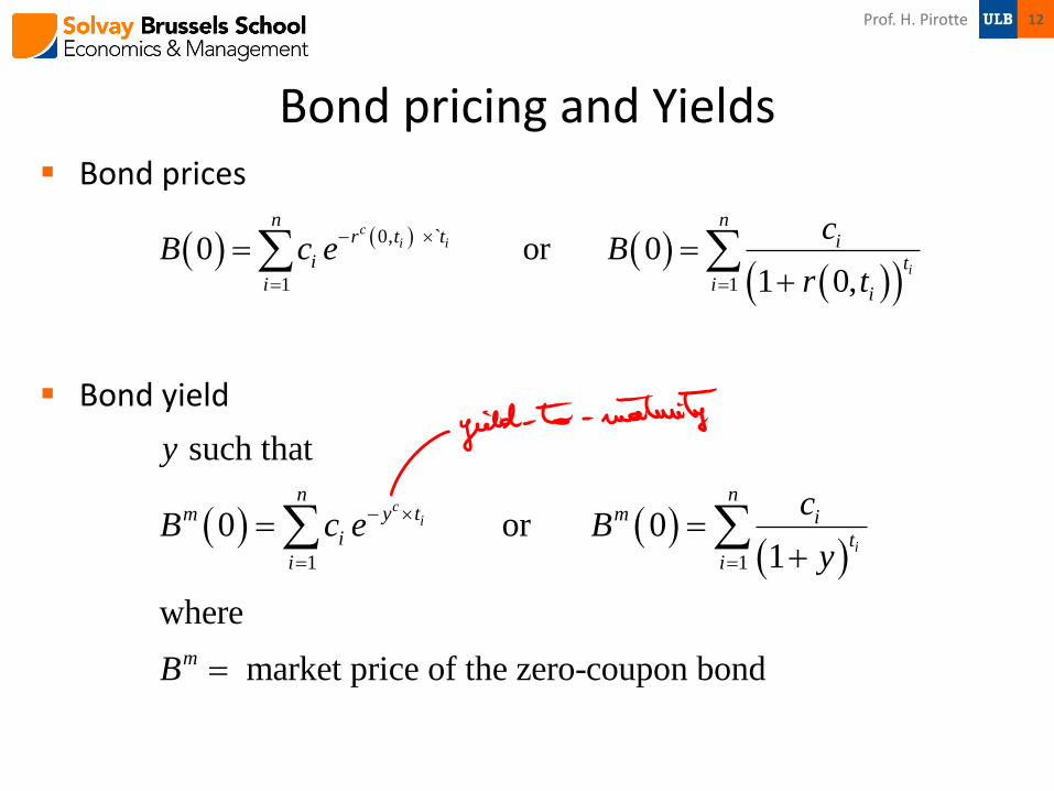
Bond pricing and Yields Bond prices

Bond yield

0, `

1 1

0 or 0 1 0,

ci i

i

n nr t t i

i ti i

i

cB c e B

r t

1 1

such that

0 or 0 1

where

market price of the zero-coupon bond

ci

i

n ny tm m i

i ti i

m

y

cB c e B

y

B

12 Prof. H. Pirotte

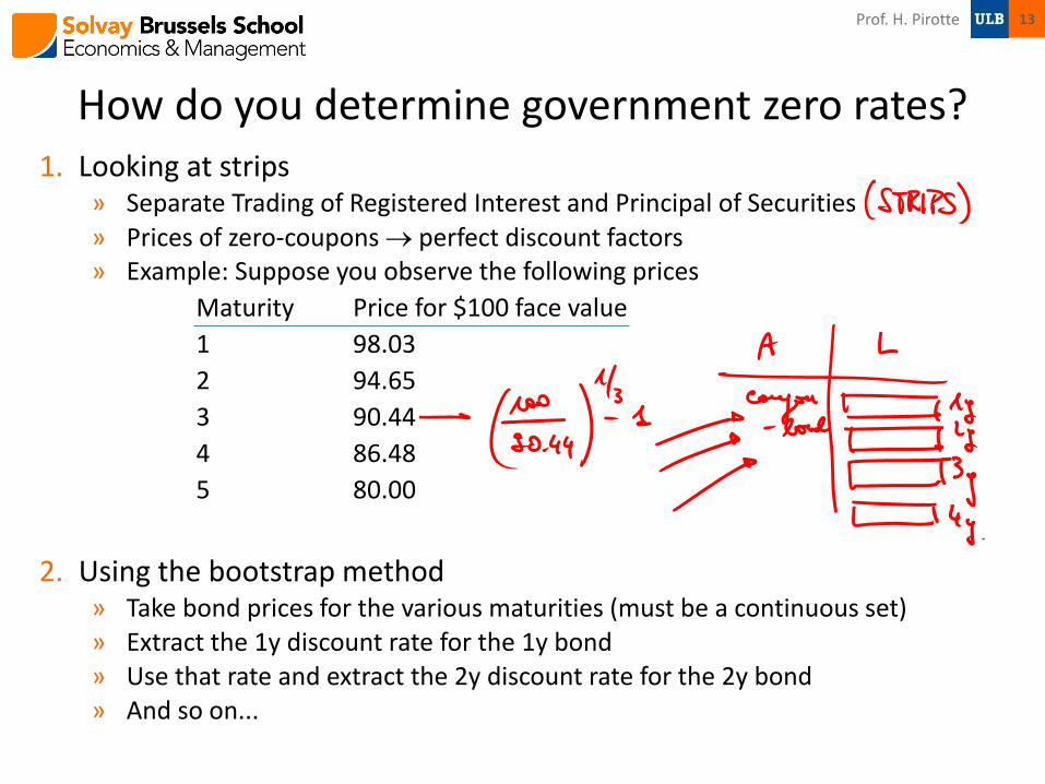
How do you determine government zero rates? 1. Looking at strips

» Separate Trading of Registered Interest and Principal of Securities » Prices of zero-coupons perfect discount factors » Example: Suppose you observe the following prices

Maturity Price for $100 face value

1 98.03

2 94.65

3 90.44

4 86.48

5 80.00

2. Using the bootstrap method » Take bond prices for the various maturities (must be a continuous set) » Extract the 1y discount rate for the 1y bond » Use that rate and extract the 2y discount rate for the 2y bond » And so on...

13 Prof. H. Pirotte

How do you determine government zero rates? (2)

3. Using discount, LIBOR, forward and swap rates » Combine these rates to generate the underlying zero-coupon curve

» Extending the LIBOR beyond one year

a) Create a yield curve that represents the rates a which AA-rated companies can borrow for periods of time longer than one year.

b) Create a yield curve to represent the future short-term borrowing rates for AA-rated companies.

In practice, we do (b).

» Example

14 Prof. H. Pirotte

The risk-free rate It is usual to assume that the LIBOR/swap yield curve provides

the risk-free rate » Treasury rates are too low

Must be purchased by a variety of institutions to fulfill regulatory requirements

The amount of capital to support an investment in T-Bills and Bonds is lower than for other similar investments

Favorable tax treatment in the US

15 Prof. H. Pirotte

Macaulays’ duration Duration

» For a zero-coupon bond: maturity = duration

» Weighted average of the times when the payments are made = weighted average of the maturities of zero-coupon bonds

Bond pricing and duration (with continuous compounding)

1

iytni

i

i

c eD t

B

BB BD y D y

B

dBB y

dy

1

1

Since ,c

i

ci

ny t

i

i

ny t

i i

i

B c e

B y c t e

16 Prof. H. Pirotte

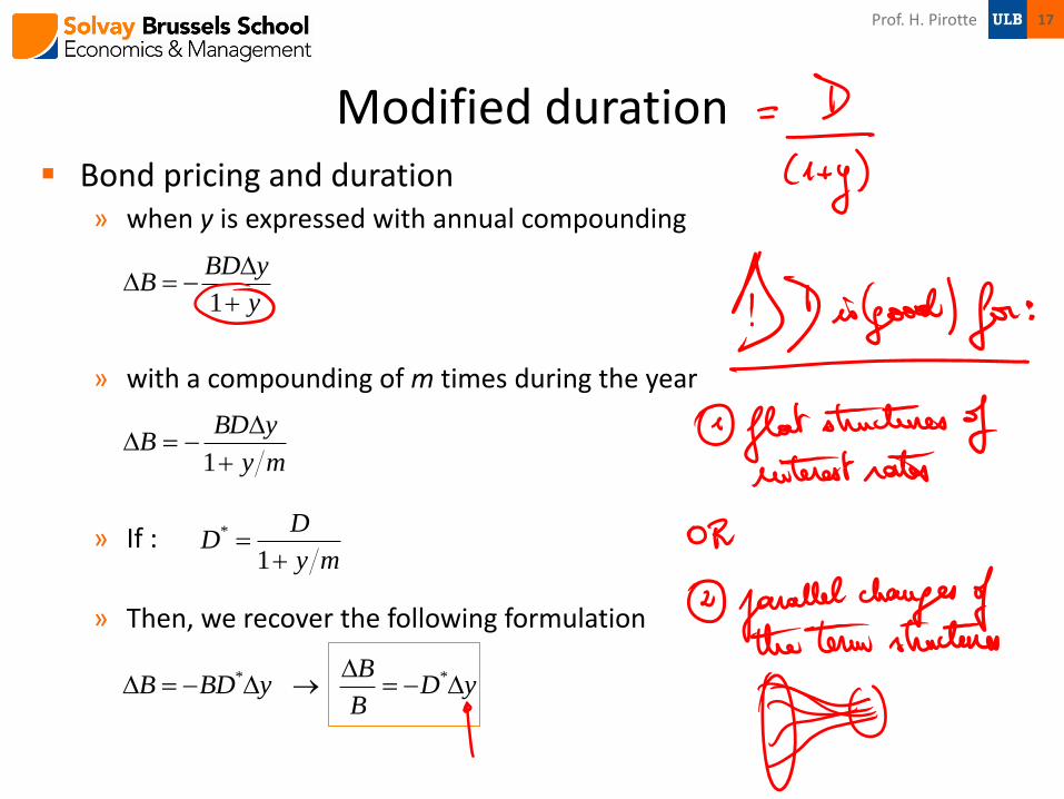
Modified duration Bond pricing and duration

» when y is expressed with annual compounding

» with a compounding of m times during the year

» If :

» Then, we recover the following formulation

my

yBDB

1

*

1

DD

y m

1

BD yB

y

* *BB BD y D y

B

17 Prof. H. Pirotte

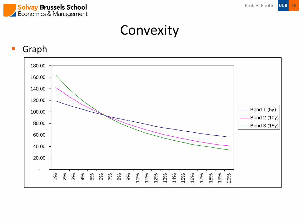
Convexity Graph

-

20.00

40.00

60.00

80.00

100.00

120.00

140.00

160.00

180.00

1%

2%

3%

4%

5%

6%

7%

8%

9%

10%

11%

12%

13%

14%

15%

16%

17%

18%

19%

20%

Bond 1 (5y)

Bond 2 (10y)

Bond 3 (15y)

18 Prof. H. Pirotte

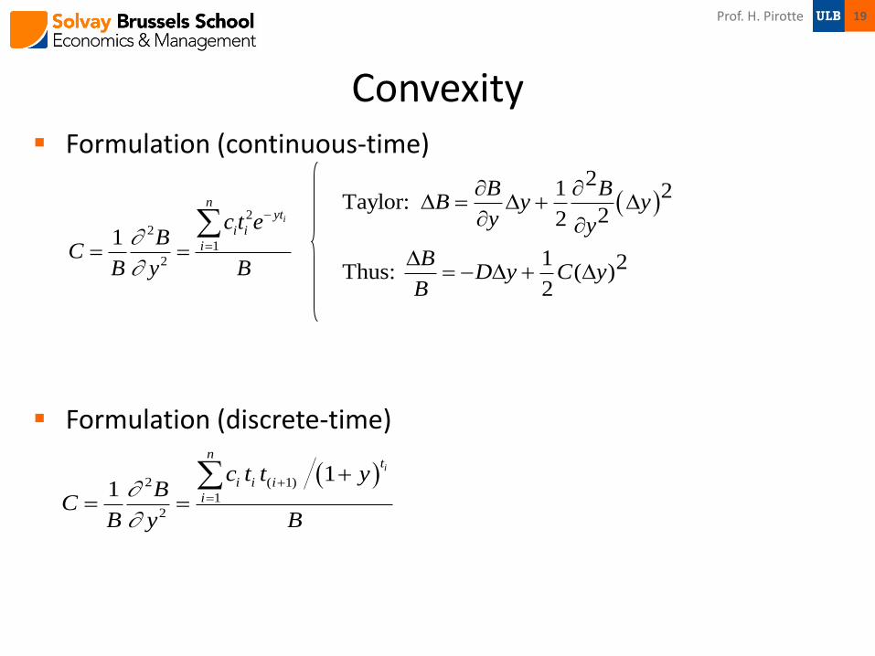
Convexity Formulation (continuous-time)

Formulation (discrete-time)

2

2

1

2

1i

nyt

i i

i

c t eB

CB y B

21 2

Taylor: 22

1 2Thus: ( )2

B BB y y

y y

BD y C y

B

2 ( 1)

1

2

11

i

nt

i i i

i

c t t yB

CB y B

19 Prof. H. Pirotte

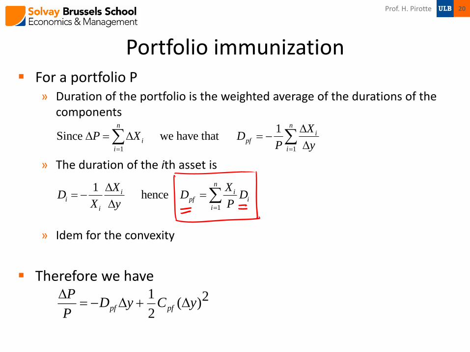
Portfolio immunization For a portfolio P

» Duration of the portfolio is the weighted average of the durations of the components

» The duration of the ith asset is

» Idem for the convexity

Therefore we have 1 2( )2

pf pf

PD y C y

P

1 1

1Since we have that

n ni

i pf

i i

XP X D

P y

1

1 hence

ni i

i pf i

ii

X XD D D

X y P

20 Prof. H. Pirotte

Problems with duration?

21 Prof. H. Pirotte

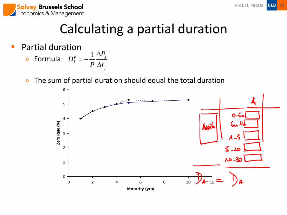
Calculating a partial duration Partial duration

» Formula

» The sum of partial duration should equal the total duration

0

1

2

3

4

5

6

0 2 4 6 8 10 12

Maturity (yrs)

Zero

Rate

(%

)1 jp

j

j

PD

P r

22 Prof. H. Pirotte

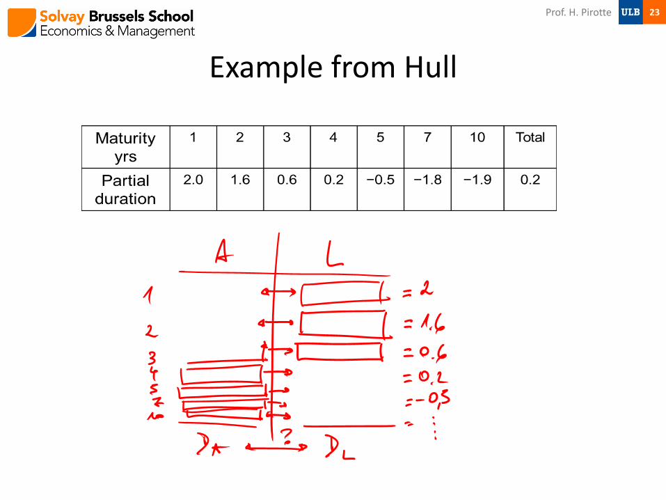
Example from Hull

23 Prof. H. Pirotte

Combining partial durations Changes of -3e, -2e, -e, 0, e , 3e, 6e for a small e in the

1,2,3,4,5,7,10 y buckets

0

1

2

3

4

5

6

7

0 2 4 6 8 10 12

Maturity (yrs)

Zero

Rate

(%

)

24 Prof. H. Pirotte

Interest rate deltas Definitions

» Change in value for 1bp parallel shift in the zero-curve

» Delta, DV01 or PVBP

» Delta = Duration * Value of the portfolio * 0.0001

» As for the partial durations, it can be done for each point on the zero-coupon curve.

» The sum of the deltas should equal the delta of the portfolio

25 Prof. H. Pirotte

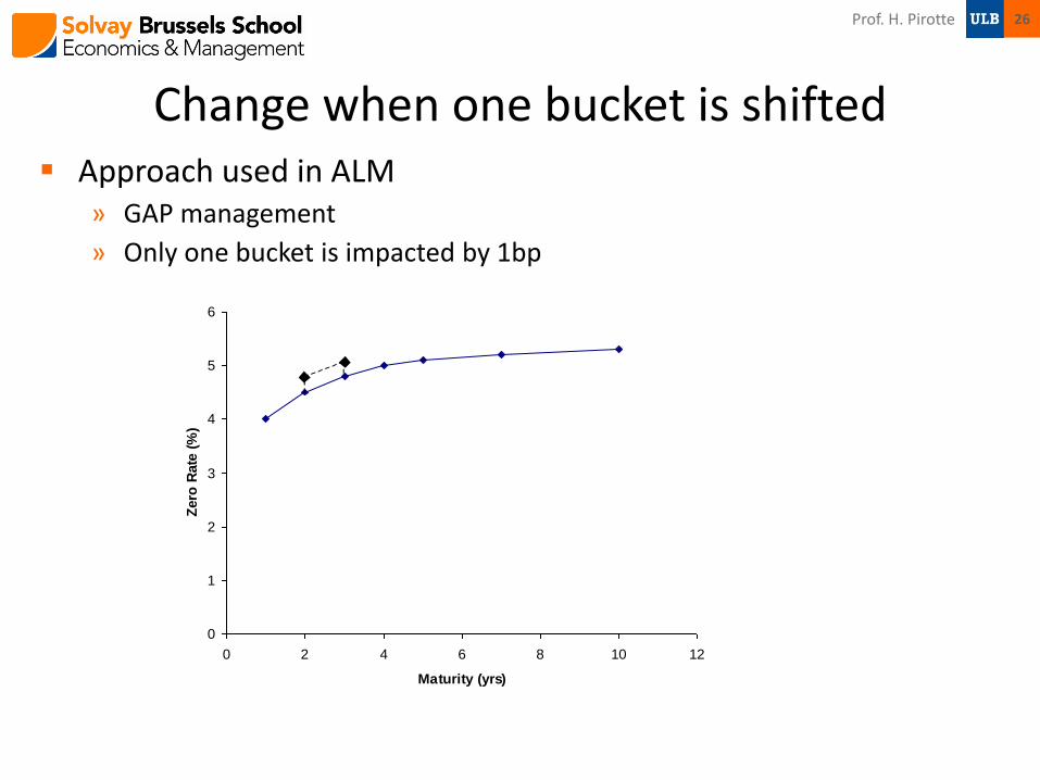
Change when one bucket is shifted Approach used in ALM

» GAP management

» Only one bucket is impacted by 1bp

0

1

2

3

4

5

6

0 2 4 6 8 10 12

Maturity (yrs)

Zero

Rate

(%

)

26 Prof. H. Pirotte

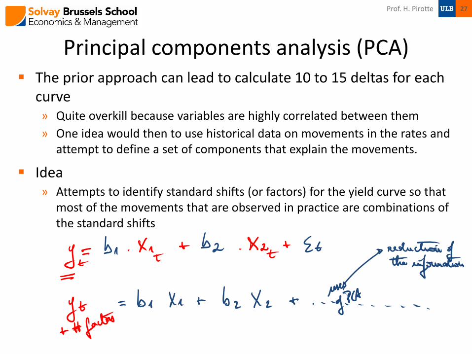
Principal components analysis (PCA) The prior approach can lead to calculate 10 to 15 deltas for each

curve » Quite overkill because variables are highly correlated between them

» One idea would then to use historical data on movements in the rates and attempt to define a set of components that explain the movements.

Idea » Attempts to identify standard shifts (or factors) for the yield curve so that

most of the movements that are observed in practice are combinations of the standard shifts

27 Prof. H. Pirotte

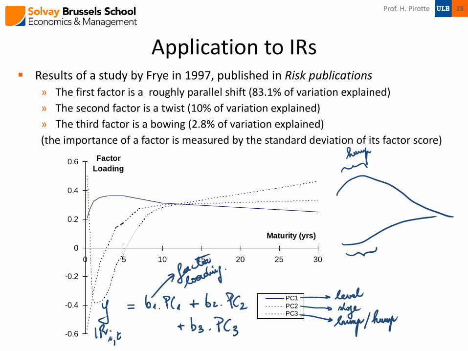
Application to IRs Results of a study by Frye in 1997, published in Risk publications

» The first factor is a roughly parallel shift (83.1% of variation explained)

» The second factor is a twist (10% of variation explained)

» The third factor is a bowing (2.8% of variation explained)

(the importance of a factor is measured by the standard deviation of its factor score)

-0.6

-0.4

-0.2

0

0.2

0.4

0.6

0 5 10 15 20 25 30

Maturity (yrs)

Factor

Loading

PC1

PC2PC3

28 Prof. H. Pirotte

Alternatives for Calculating Multiple Deltas Shift individual points on the yield curve by one basis point

Shift segments of the yield curve by one basis point

Shift quotes on instruments used to calculate the yield curve

Calculate deltas with respect to the shifts given by a principal components analysis.

29 Prof. H. Pirotte

Gamma for Interest Rates Gamma has the form

where xi and xj are yield curve shifts considered for delta

To avoid too many numbers being produced one possibility is consider only i = j

Another is to consider only parallel shifts in the yield curve

Another is to consider the first two or three types of shift given by a principal components analysis

Prof. H. Pirotte 30

ji xx

2

Vega for Interest Rates One possibility is to make the same change to all interest rate

implied volatilities. (However implied volatilities for long-dated options change by less than those for short-dated options.)

Another is to do a principal components analysis on implied volatility changes.

Prof. H. Pirotte 31

References Books & Notes

» RMH: Chap. 7

» Don Chance teaching notes

32 Prof. H. Pirotte