Risk Management and Bond Structuring: A Marriage Overdue · • Although bond structuring strategies and risk management strategies are interdependent, analysts have traditionally

Copyright © 2008 Intuitive Analytics LLC. All Rights Reserved. First Edition, March 2008 www.intuitive-analytics.com

Risk Management and Bond

Structuring:

A Marriage Overdue

A White Paper from

Intuitive Analytics

by Peter Orr, CFA

• Although bond structuring strategies and risk management strategies are interdependent, analysts have traditionally used separate, disparate tools for these processes, with suboptimal results.

• New analytics marry these processes by evaluating funding and risk decisions together.

• Tax-exempt issuers can now greatly lower their expected cost per unit of risk by evaluating both bond and derivative strategies within a single problem statement.

2

Summary “Better a rough answer to the right question than an exact answer to the wrong one.”

-Anonymous (possibly Lord Kelvin)

While financial markets and computing power have evolved dramatically over the last twenty years, technological developments in tax-exempt financial structuring have not kept pace. Most notably, issuers are forced to make bond structuring decisions (determining the type of debt, amortization schedule, and sources and uses of funding) using analytics that are separate and apart from their risk management analysis (weighing the size and type of market risks assumed, the suitability of capital market tools such as swaps and their effect on cost and risk, the and effects of new risks on existing capital structure).

Traditionally, analysts employ specific, financial structuring software and spreadsheets for the bond structuring component, and ad hoc analysis such as asset/liability management tools, for the risk management problem. The lack of a single decision tool results in suboptimal decision-making and financing strategies with an unnecessarily high expected cost per unit of risk.

This paper describes a new method for integrating bond and derivative structuring strategies within a unified problem statement and with a straightforward objective: minimize expected borrowing cost given a calculated constraint on cash flow risk (Cash Flow at Risk or “CFaR”). The result of this method is that issuers of tax-exempt securities can now evaluate both bond (cash) and derivative (synthetic) strategies within a single, coordina ted, comprehensive framework.

Two case studies demonstrate the novelty and advantages of this overdue marriage between tools for bond structuring and risk management:

• $200 million New Money borrowing – At the same level of risk, this results in $12.4 million expected present value benefit relative to a more traditional structure.

• $200 million New Money borrowing with $20 million cash (earning LIBOR) – In this case, we calculate the cost of using at least $100 million of underlying fixed-rate bonds in the solution. The expected capital cost increases by 0.19% explicitly pricing this constraint.

3

History “History will be kind to me for I intend to write it .”

-Winston Churchill

Financial innovation and natural market evolution have brought an ever-growing smorgasbord of products and financing vehicles to the tax-exempt market over the course of the last 30 years:

• Variable-rate Demand Bonds were developed in response to the Federal Reserve experiment of the late 1970s and early 1980s when yields on Treasury Bills exceeded 19%

• Interest rate swaps sprang from a 1981 transaction between the World Bank and IBM

• The Tax Reform Act of 1986 ushered in an era of advance refunding limitations

• The U.S. Treasury created State and Local Government Securities to accommodate yield restricted investments.

• Securitization in tax-exempt securities led to Tender Option Bond programs and various spin-offs and derivatives.

Along with this growing structural buffet comes a similarly diverse list of market exposures:

• Taxable (LIBOR) and tax-exempt (SIFMA index1) interest rates and the ratio between them

• Constant Maturity Swap rates • Basket index exposures • Consumer Price Index risk • Currency variability (in certain circumstances)

Despite these watershed changes in the number of and ways to assume financial risks, the market has failed to provide significant advances in the means to structure new borrowings in the tax-exempt market. In fact, the basic types of bond structuring solutions have not changed materially in well over a decade.

In two case studies, this paper explores the result of marrying the capabilities of traditional bond structuring software to the features of high-quality risk management analytics, allowing the explicit integration of risk metrics such as Cash Flow at Risk2 (CFaR) into the new financing problem.

1 The Securities Industry and Financial Markets Association, formerly known as the Bond Market Association (BMA) Index.

2 See description of CFaR in “Cashflow at Risk (CFaR) for Tax-Exempt Liability Management”. Intuitive Analytics, September 2006.

4

Background “To be sure of hitting the target, shoot first, and call whatever you hit the target.”

-Ashleigh Brilliant

Currently, when an issuer with a funding need investigates the structure of a new borrowing, bankers and/or advisors offer analysis and different debt modes: callable and non-callable fixed-rate bonds, variable-rate demand bonds, auction rate securities, and “direct lending” alternatives, among others. Ultimately, an analyst will use bond structuring software, a spreadsheet, or some combination of the two to create a bond solution (sources and uses of funds, principal amortizations, debt service schedule, et al.). At a minimum, this solution will satisfy a bond sizing target and a debt service “shape” objective, such as level expected3 principal and interest payments.

Similarly, as markets change and risk management opportunities present themselves, issuers may explore swap or derivative strategies to reduce expected cost or risk. In turn, the banker or advisor may employ some sort of risk management analytic (often called “Asset/Liability Management” or “ALM” studies) to illuminate risk characteristics of the strategy and help inform the issuer’s decision.

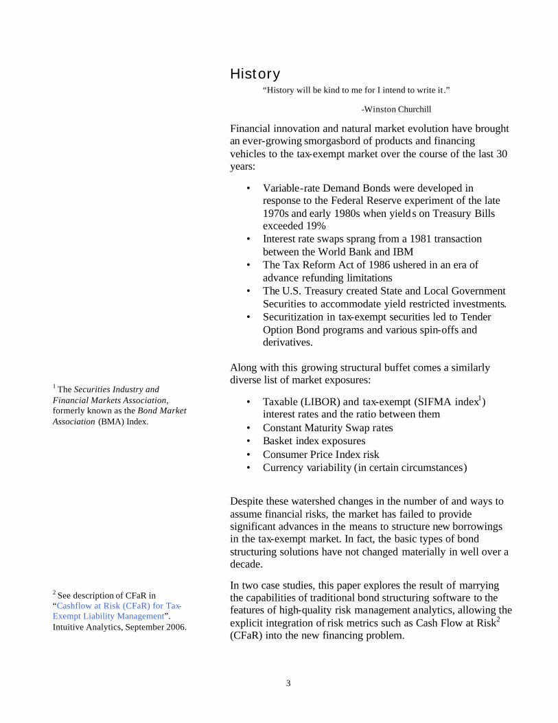
Figure 1 depicts, with intentionally sharpened contrast, the separation between bond structuring analysis and risk management analysis. In practice, the situation may be grayer. Nonetheless, we believe strongly that, for optimal decision-making, models of real-world problems should capture as many integrated dynamics of the real world as possible.

The two case studies that follow show how a single model provides comprehensive solutions involving fixed and variable-rate bonds and swaps. The model achieves the low-cost debt service objective while satisfying a constraint on cash flow risk.

Case Study 1 – $200 Million in New Money, Efficiently The Board of a new tax-exempt entity (“NewIssuer”) has approved a policy of 50% variable-rate debt. NewIssuer needs to raise $200 million for a new project and has no existing debt. NewIssuer is looking to achieve level expected debt service over 30 years.

Before exploring the 50% variable target, let us first look at a fixed-rate issue. A 30-year, fixed-rate, level debt service structure would generate an overall issue yield of 4.43%4. The expected cash flow variability of fixed-rate debt is zero (for the

FundingDecision

BondAnalytics

Risk Analytics

BondAnalyst

DerivativesAnalyst

Uncoordinated Financial Strategy


RiskRiskDecisionDecision

FundingDecision

BondAnalytics

Risk Analytics

BondAnalyst

DerivativesAnalyst



RiskRiskDecisionDecision

Figure 1 - Separate Funding and Risk Analyses

3 The word “expected” is important in this context. When structuring variable rate bonds, the analyst often assumes (heroically) a static short-term interest rate level for the term of the analysis, sometimes 30 years or more.

4 Market interest rates as of December 15, 2007

5

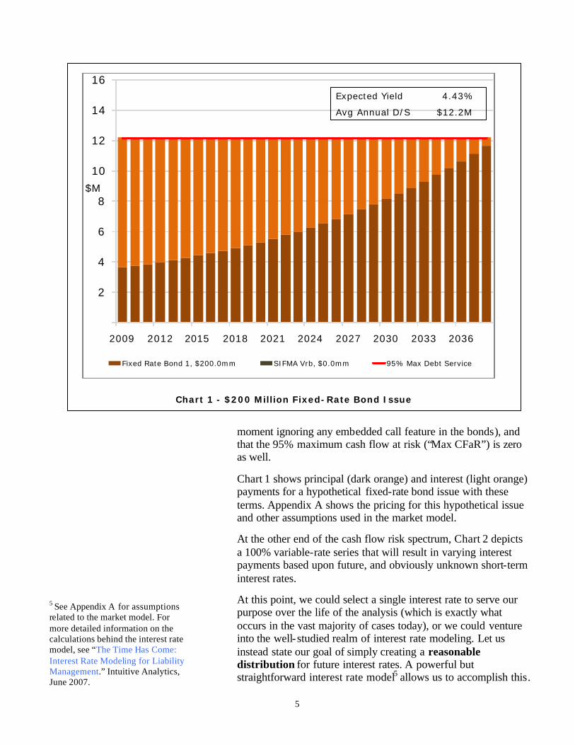
moment ignoring any embedded call feature in the bonds), and that the 95% maximum cash flow at risk (“Max CFaR”) is zero as well.

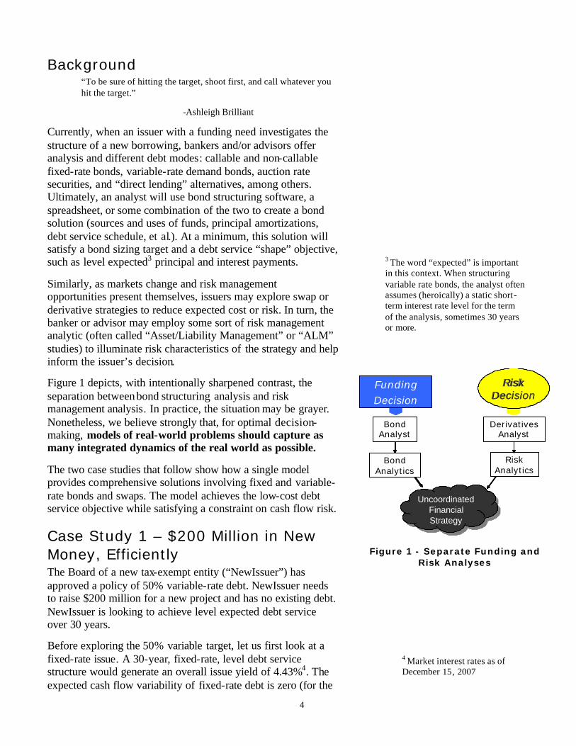
Chart 1 shows principal (dark orange) and interest (light orange) payments for a hypothetical fixed-rate bond issue with these terms. Appendix A shows the pricing for this hypothetical issue and other assumptions used in the market model.

At the other end of the cash flow risk spectrum, Chart 2 depicts a 100% variable-rate series that will result in varying interest payments based upon future, and obviously unknown short-term interest rates.

At this point, we could select a single interest rate to serve our purpose over the life of the analysis (which is exactly what occurs in the vast majority of cases today), or we could venture into the well-studied realm of interest rate modeling. Let us instead state our goal of simply creating a reasonable distribution for future interest rates. A powerful but straightforward interest rate model5 allows us to accomplish this.

2

4

6

8

10

12

14

16

2009 2012 2015 2018 2021 2024 2027 2030 2033 2036

Fixed Rate Bond 1, $200.0mm SIFMA Vrb, $0.0mm 95% Max Debt Service

Expected Yield 4.43%

Avg Annual D/S $12.2M

$M

Chart 1 - $200 Million Fixed-Rate Bond Issue

5 See Appendix A for assumptions related to the market model. For more detailed information on the calculations behind the interest rate model, see “The Time Has Come: Interest Rate Modeling for Liability Management.” Intuitive Analytics, June 2007.

6

Based on the simple SIFMA model we employ, the expected yield on this 100% variable-rate issue is 3.45%, roughly 97 basis points below the yield on the pure fixed-rate issue. However, there is cash flow variability in the 100% variable-rate structure; 95% Annual CFaR equals $4.37 million. In other words, the maximum difference across all years in the analysis between expected annual debt service and 95% worst-case debt service, is $4.37 million.

Chart 2 also shows the 100% variable-rate debt service schedule. The darker green shade is principal; the lighter is interest. Notice that the red line, indicating the 95th percentile for debt service payments, rises initially with interest rate uncertainty, but then begins to decline as principal is retired. The decline in risk is a natural consequence of interest becoming a smaller and smaller proportion of each total debt service payment.

2

4

6

8

10

12

14

16

2009 2012 2015 2018 2021 2024 2027 2030 2033 2036


$M

95% Max CFaR = $4.37mm


Average Ann D/S $10.81M

Chart 2 - $200 Million Variable-Rate Bond Issue

7

Baseline Scenario 1 With an approved 50-50 fixed/variable policy, NewIssuer splits the structures in half, leaving a $100 million amortization over thirty years for each of the fixed and variable-rate pieces. Chart 3 shows the resulting principal amortization for each of the fixed and variable-rate bonds. This pro-rata scenario will serve as the baseline of comparison for the three scenarios that follow and complete this case study.

The orange reflects the fixed amortization and the green shows the variable-rate piece. In each case, the darker shade indicates principal; the lighter is interest. Notice that CFaR is exactly half the amount it was in the 100% variable-rate structure shown in Chart 2.

2

4

6

8

10

12

14

16

2009 2012 2015 2018 2021 2024 2027 2030 2033 2036


95% CFaR = $2.19mm



$M

Chart 3 - $200 Million, 50% Variable – Pro-rata Amortization

8

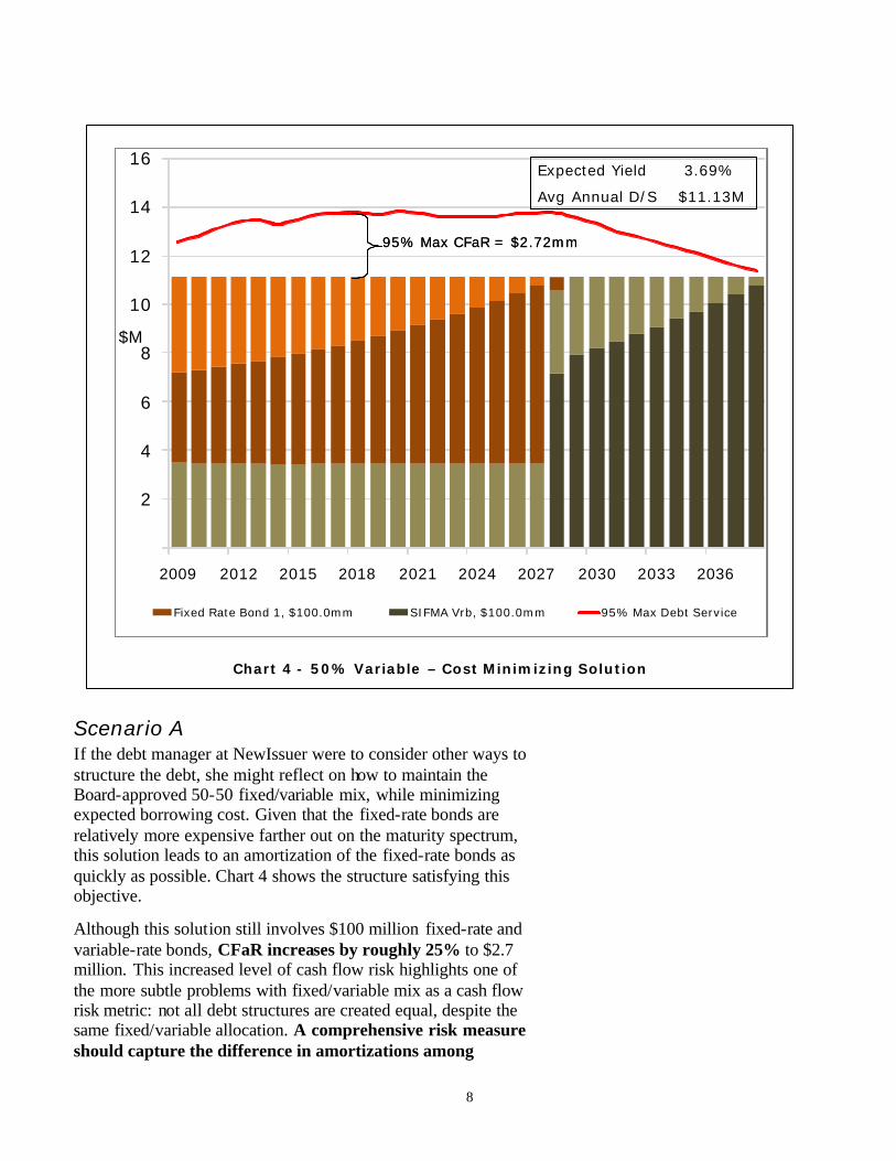
Scenario A If the debt manager at NewIssuer were to consider other ways to structure the debt, she might reflect on how to maintain the Board-approved 50-50 fixed/variable mix, while minimizing expected borrowing cost. Given that the fixed-rate bonds are relatively more expensive farther out on the maturity spectrum, this solution leads to an amortization of the fixed-rate bonds as quickly as possible. Chart 4 shows the structure satisfying this objective.

Although this solution still involves $100 million fixed-rate and variable-rate bonds, CFaR increases by roughly 25% to $2.7 million. This increased level of cash flow risk highlights one of the more subtle problems with fixed/variable mix as a cash flow risk metric: not all debt structures are created equal, despite the same fixed/variable allocation. A comprehensive risk measure should capture the difference in amortizations among

2

4

6

8

10

12

14

16

2009 2012 2015 2018 2021 2024 2027 2030 2033 2036


95% Max CFaR = $2.72mm95% Max CFaR = $2.72mm



$M

Chart 4 - 50% Variable – Cost Minimizing Solution

9

alternatives; unfortunately, the fixed/variable mix metric, as commonly defined, cannot capture it.

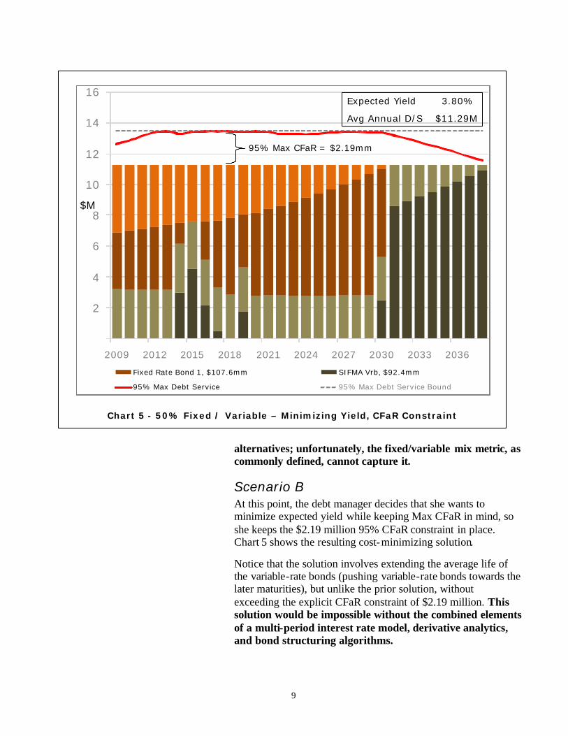
Scenario B At this point, the debt manager decides that she wants to minimize expected yield while keeping Max CFaR in mind, so she keeps the $2.19 million 95% CFaR constraint in place. Chart 5 shows the resulting cost-minimizing solution.

Notice that the solution involves extending the average life of the variable-rate bonds (pushing variable-rate bonds towards the later maturities), but unlike the prior solution, without exceeding the explicit CFaR constraint of $2.19 million. This solution would be impossible without the combined elements of a multi-period interest rate model, derivative analytics, and bond structuring algorithms.

2

4

6

8

10

12

14

16

2009 2012 2015 2018 2021 2024 2027 2030 2033 2036

Fixed Rate Bond 1, $107.6mm SIFMA Vrb, $92.4mm

95% Max Debt Service 95% Max Debt Service Bound



$M


Chart 5 - 50% Fixed / Variable – Minimizing Yield, CFaR Constraint

10

The debt manager at NewIssuer has now taken a critical conceptual step: a product type, such as variable-rate, does not drive a comprehensive risk measure. The components of a complete risk measure are the inherent variability of one or more different types of underlying cash flow risks and their expected co-movement.6

With this step taken, the overall financing objective becomes clear, not only in theory but in practice:

For a specified level of risk, minimize expected cost, or

For a given level of expected cost, minimize risk.

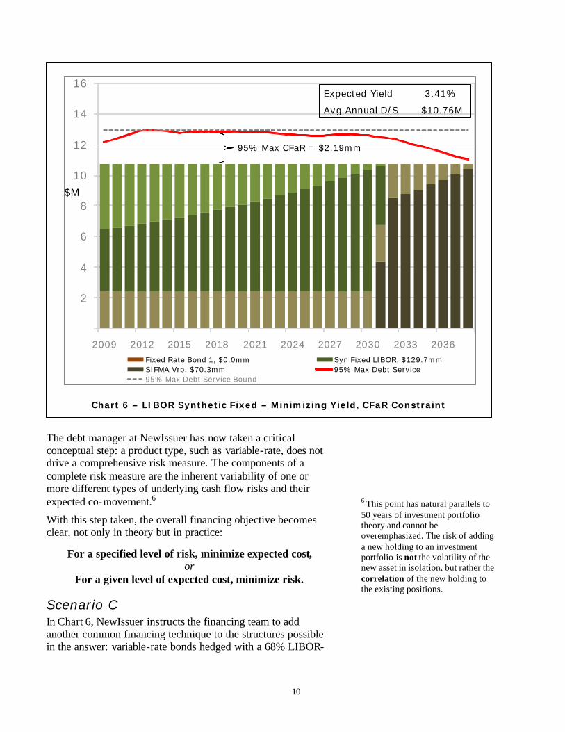
Scenario C In Chart 6, NewIssuer instructs the financing team to add another common financing technique to the structures possible in the answer: variable-rate bonds hedged with a 68% LIBOR-

6 This point has natural parallels to 50 years of investment portfolio theory and cannot be overemphasized. The risk of adding a new holding to an investment portfolio is not the volatility of the new asset in isolation, but rather the correlation of the new holding to the existing positions.

2

4

6

8

10

12

14

16

2009 2012 2015 2018 2021 2024 2027 2030 2033 2036Fixed Rate Bond 1, $0.0mm Syn Fixed LIBOR, $129.7mmSIFMA Vrb, $70.3mm 95% Max Debt Service95% Max Debt Service Bound

© 2007 Intuitive Analytics LLCAll rights reserved



$M


Chart 6 – LIBOR Synthetic Fixed – Minimizing Yield, CFaR Constraint

11

based interest rate swap, often called a “LIBOR synthetic fixed” structure.

As shown in the chart, with this third debt mode available the solution takes better advantage of the $2.19 million CFaR risk budget and reduces the expected borrowing cost to 3.41%, which is actually 5 basis points lower than the expected cost of 100% variable-rate bonds. Note that the solution is lower expected cost of funding at half the level of 95% CFaR of the pure variable-rate structure. How is this possible? The average

swap rates in the 68% LIBOR swap solution are lower than the expected yield on the variable-rate bonds, leading the manager to the holy grail of solutions – lower risk and lower cost.

Table 1 summarizes and compares the statistics from the various solutions in Case Study 1.

Notice that the “50% Variable/Capital” alternative had lower cost than the pro-rata solution but with much higher cash flow risk at over $2.7 million CFaR�. The “50% Variable /Bounded CFaR” delivered about 14 basis points� of expected cost savings over the pro-rata case, which represented approximately $199,000 annually in expected cash flow benefit. However, the last alternative, which includes the 68% LIBOR synthetic fixed structure, is by far the optimal scenario: it delivered $12.7 million� in lower expected cost than the variable-rate bonds, at half the level of risk.

Case Study 2 – A Second Marriage, With Assets

“Take calculated risks. This is quite different from being rash.”

50% Variable 50% Variable 50% Variable w/ Syn Fixed LIBORPro-rata Capital Bounded CFaR Bounded CFaR

Yield 3.945% 3.686% 3.803% 3.412%Average D/S 11,493,769 11,132,289 11,294,790 10,757,414

95% Max CFaR 2,185,391 2,718,912 2,185,391 2,185,391 Avg $ Volatility 768,232 1,102,666 962,632 932,428

Overall Average Life 18.3 18.3 18.4 17.9 Avg Annual Benefit - 361,480 198,979 736,355

Bps Benefit - 26 14 53 PV Difference @ 4% - 6,250,721 3,440,756 12,733,076

Benefit % of Par - 3.1% 1.7% 6.4%

Table 1 - Summary Statistics for Four Scenarios, Case Study 1

12

-George S. Patton

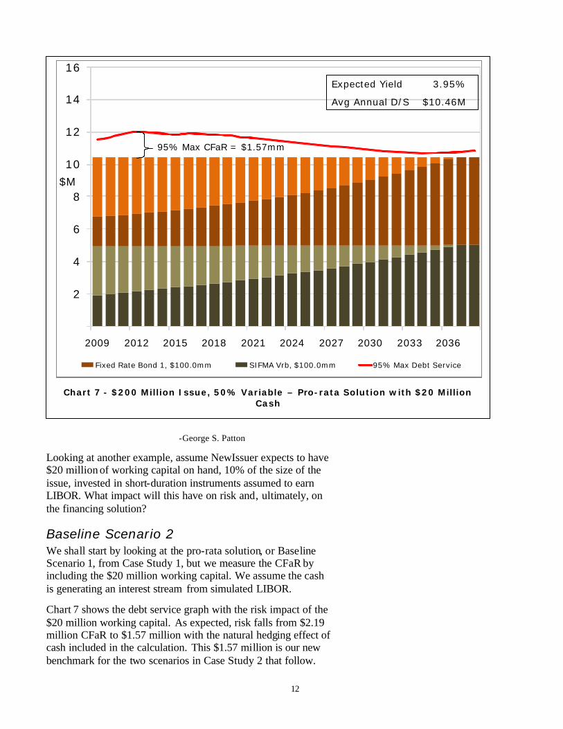
Looking at another example, assume NewIssuer expects to have $20 million of working capital on hand, 10% of the size of the issue, invested in short-duration instruments assumed to earn LIBOR. What impact will this have on risk and, ultimately, on the financing solution?

Baseline Scenario 2 We shall start by looking at the pro-rata solution, or Baseline Scenario 1, from Case Study 1, but we measure the CFaR by including the $20 million working capital. We assume the cash is generating an interest stream from simulated LIBOR.

Chart 7 shows the debt service graph with the risk impact of the $20 million working capital. As expected, risk falls from $2.19 million CFaR to $1.57 million with the natural hedging effect of cash included in the calculation. This $1.57 million is our new benchmark for the two scenarios in Case Study 2 that follow.

2

4

6

8

10

12

14

16

2009 2012 2015 2018 2021 2024 2027 2030 2033 2036





$M

Chart 7 - $200 Million Issue, 50% Variable – Pro-rata Solution with $20 Million Cash

13

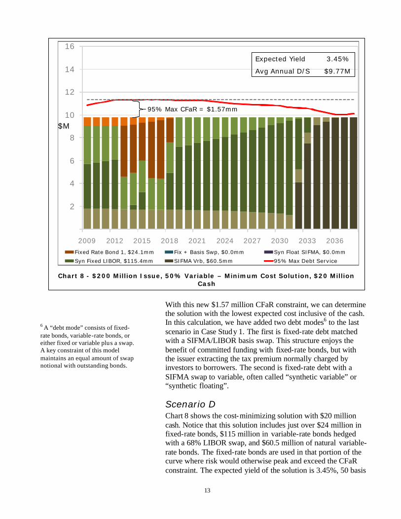
With this new $1.57 million CFaR constraint, we can determine the solution with the lowest expected cost inclusive of the cash. In this calculation, we have added two debt modes6 to the last scenario in Case Study 1. The first is fixed-rate debt matched with a SIFMA/LIBOR basis swap. This structure enjoys the benefit of committed funding with fixed-rate bonds, but with the issuer extracting the tax premium normally charged by investors to borrowers. The second is fixed-rate debt with a SIFMA swap to variable, often called “synthetic variable” or “synthetic floating”.

Scenario D Chart 8 shows the cost-minimizing solution with $20 million cash. Notice that this solution includes just over $24 million in fixed-rate bonds, $115 million in variable-rate bonds hedged with a 68% LIBOR swap, and $60.5 million of natural variable-rate bonds. The fixed-rate bonds are used in that portion of the curve where risk would otherwise peak and exceed the CFaR constraint. The expected yield of the solution is 3.45%, 50 basis

2

4

6

8

10

12

14

16

2009 2012 2015 2018 2021 2024 2027 2030 2033 2036Fixed Rate Bond 1, $24.1mm Fix + Basis Swp, $0.0mm Syn Float SIFMA, $0.0mm

Syn Fixed LIBOR, $115.4mm SIFMA Vrb, $60.5mm 95% Max Debt Service

$M




Chart 8 - $200 Million Issue, 50% Variable – Minimum Cost Solution, $20 Million Cash

6 A “debt mode” consists of fixed-rate bonds, variable-rate bonds, or either fixed or variable plus a swap. A key constraint of this model maintains an equal amount of swap notional with outstanding bonds.

14

points lower than the pro-rata base case above, but at the same level of Max CFaR.

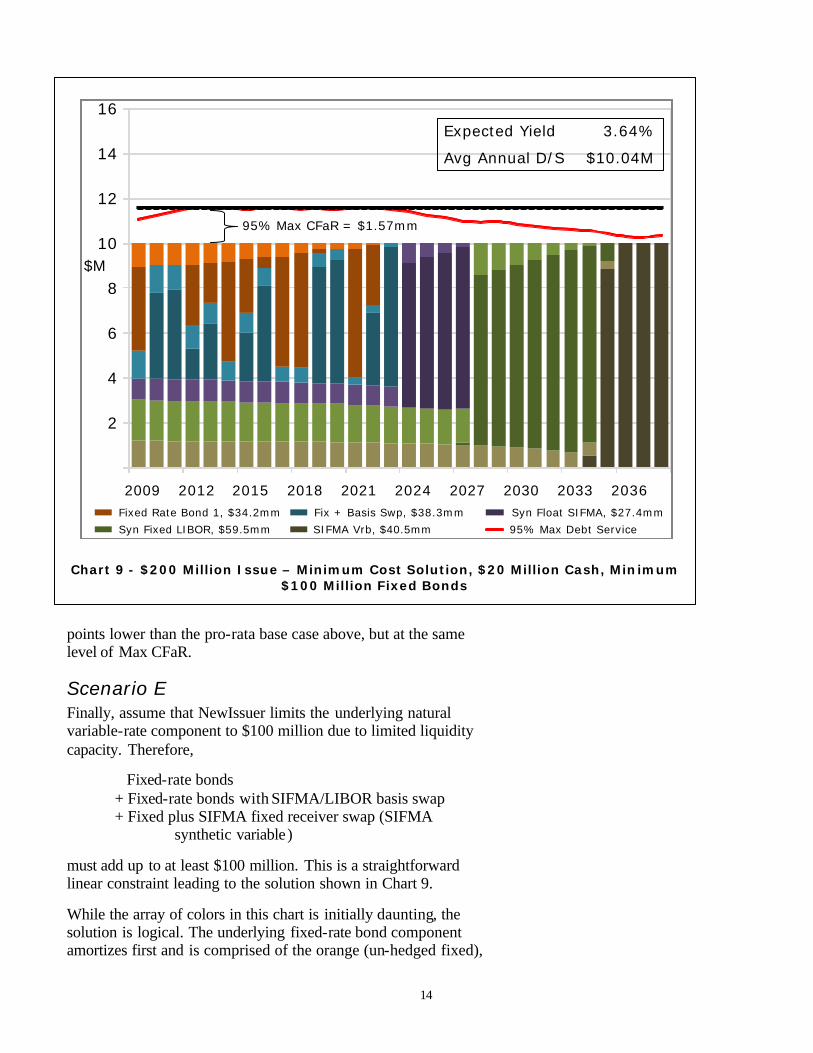
Scenario E Finally, assume that NewIssuer limits the underlying natural variable-rate component to $100 million due to limited liquidity capacity. Therefore,

Fixed-rate bonds + Fixed-rate bonds with SIFMA/LIBOR basis swap + Fixed plus SIFMA fixed receiver swap (SIFMA

synthetic variable)

must add up to at least $100 million. This is a straightforward linear constraint leading to the solution shown in Chart 9.

While the array of colors in this chart is initially daunting, the solution is logical. The underlying fixed-rate bond component amortizes first and is comprised of the orange (un-hedged fixed),

2

4

6

8

10

12

14

16






$M

2

4

6

8

10

12

14

16



2

4

6

8

10

12

14

16






$M

Chart 9 - $200 Million Issue – Minimum Cost Solution, $20 Million Cash, Minimum $100 Million Fixed Bonds

15

blue (fixed with SIFMA/LIBOR basis swap) and purple (fixed with SIFMA swap to variable). Through 2024, the amortization is natural- fixed and fixed with a basis swap. At that point, the risk-adjusted appeal of the synthetic variable kicks in and is a component of the solution through 2028. From there, the LIBOR synthetic fixed (green) and un-hedged variable-rate bonds (brown) round out the structure.

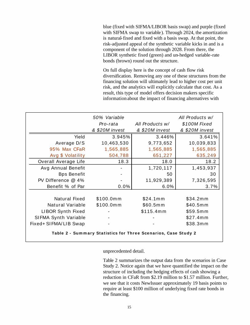
On full display here is the concept of cash flow risk diversification. Removing any one of these structures from the financing solution will ultimately lead to higher cost per unit risk, and the analytics will explicitly calculate that cost. As a result, this type of model offers decision makers specific information about the impact of financing alternatives with

unprecedented detail.

Table 2 summarizes the output data from the scenarios in Case Study 2. Notice again that we have quantified the impact on the structure of including the hedging effects of cash showing a reduction in CFaR from $2.19 million to $1.57 million. Further, we see that it costs NewIssuer approximately 19 basis points to require at least $100 million of underlying fixed rate bonds in the financing.

50% Variable All Products w/ Pro-rata All Products w/ $100M Fixed

& $20M invest & $20M invest & $20M investYield 3.945% 3.446% 3.641%

Average D/S 10,463,530 9,773,652 10,039,833 95% Max CFaR 1,565,885 1,565,885 1,565,885 Avg $ Volatility 504,788 651,227 635,249

Overall Average Life 18.3 18.0 18.2 Avg Annual Benefit - 1,720,117 1,453,937

Bps Benefit - 50 30 PV Difference @ 4% - 11,929,389 7,326,595

Benefit % of Par 0.0% 6.0% 3.7%

Natural Fixed $100.0mm $24.1mm $34.2mmNatural Variable $100.0mm $60.5mm $40.5mm

LIBOR Synth Fixed - $115.4mm $59.5mmSIFMA Synth Variable - - $27.4mm

Fixed+SIFMA/LIB Swap - - $38.3mm

Table 2 - Summary Statistics for Three Scenarios, Case Study 2

16

Analytics used to solve these types of problems should possess certain features that capture the real world dynamics of the problem. Analytics for this type of solution should:

• Include a market model capturing expected levels, volatilities and correlations of all relevant cash flow risk elements.

• Incorporate both fixed- and variable-rate bonds. • Generate comprehensive cash flows for all instruments,

bonds and derivatives using the market model above. • Accommodate all standard bond solutions – level,

uniform, proportional, accelerated, deferred and fill. • Calculate both absolute and relative cash flow risk

metrics and specify them as risk constraints within the solution.

• Support bond denominations7

Living Happily Ever After “There are risks and costs to a program of action, but they are far less than the long-range risks and costs of comfortable inaction.”

-John F. Kennedy

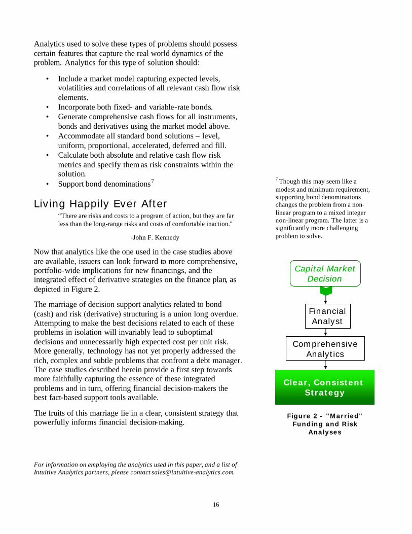
Now that analytics like the one used in the case studies above are available, issuers can look forward to more comprehensive, portfolio-wide implications for new financings, and the integrated effect of derivative strategies on the finance plan, as depicted in Figure 2.

The marriage of decision support analytics related to bond (cash) and risk (derivative) structuring is a union long overdue. Attempting to make the best decisions related to each of these problems in isolation will invariably lead to suboptimal decisions and unnecessarily high expected cost per unit risk. More generally, technology has not yet properly addressed the rich, complex and subtle problems that confront a debt manager. The case studies described herein provide a first step towards more faithfully capturing the essence of these integrated problems and in turn, offering financial decision-makers the best fact-based support tools available.

The fruits of this marriage lie in a clear, consistent strategy that powerfully informs financial decision-making.

For information on employing the analytics used in this paper, and a list of Intuitive Analytics partners, please contact [email protected].

7 Though this may seem like a modest and minimum requirement, supporting bond denominations changes the problem from a non-linear program to a mixed integer non-linear program. The latter is a significantly more challenging problem to solve.

Clear, Consistent Strategy

FinancialAnalyst

Capital MarketCapital MarketDecisionDecision

ComprehensiveAnalytics

Figure 2 - "Married" Funding and Risk

Analyses

17

About the Author Peter Orr founded Intuitive Analytics in 2005. Prior to Intuitive Analytics, he designed and developed analytics that have been used broadly within JPMorgan public finance investment banking, swaps, and risk management. He has served as vice chair of the Bond Market Association's New Products Committee and chair of its Financial Products Committee. Copyright © 2008 Intuitive Analytics LLC. All Rights Reserved. First Edition, March 2008 Intuitive Analytics LLC 190 N. 10th St, Suite 313 Brooklyn, NY 11211 646.202.9446 www.intuitive-analytics.com

Risk Management and Bond Structuring: A Marriage Overdue

18

Appendix A

The market model employed in this paper to create distributions for LIBOR and SIFMA/LIBOR (SIFMA is generated by multiplying the two) is a generalized form of Vasicek interest rate model with mean reverting drift and lognormal volatility term. The inputs used in this paper are shown below. For more information on the inner-workings of this powerful but straightforward model, see “The Time Has Come: Interest Rate Modeling for Liability Management” available at www.intuitive-analytics.com.

Basic Cash Flow Factor Inputs

Model Initial AverageFactor # Name Type Rate Rate Volatility

1 LIBOR Rate 5.15% 5.15% 24.00%2 BMA/LIB Ratio 68.00% 68.00% 10.00%

10Y LIB Rate 5.00% 6.50% 18.00%

Factor Correlations

Factor # Name LIBOR BMA/LIB1 LIBOR 1.000 -0.262 0.0952 BMA/LIB -0.262 1.000 -0.196

0.095 -0.196 1.000

Risk Management and Bond Structuring: A Marriage Overdue Intuitive Analytics

19

Appendix A (continued)

The market factors described on the prior page lead to a modeled form of expected capital cost for each “debt mode” used in this paper. For each of the “debt modes” used in this paper, the table below shows these expected capital costs. A chart of these costs follows on the next page.

Year SIFMA

Vrb Syn Fixed LIBOR

Syn Fixed SIFMA

Fix + Basis Swp

Fixed Rate Bond 1

2009 3.48% 2.99% 3.54% 3.16% 3.15% 2010 3.47% 2.79% 3.82% 3.24% 3.24% 2011 3.47% 2.82% 3.84% 3.29% 3.30% 2012 3.46% 2.89% 3.81% 3.34% 3.36% 2013 3.46% 2.97% 3.80% 3.41% 3.44% 2014 3.46% 3.05% 3.79% 3.49% 3.52% 2015 3.45% 3.12% 3.79% 3.56% 3.60% 2016 3.45% 3.18% 3.81% 3.63% 3.69% 2017 3.45% 3.23% 3.84% 3.72% 3.79% 2018 3.45% 3.27% 3.88% 3.80% 3.88% 2019 3.45% 3.31% 3.92% 3.88% 3.98% 2020 3.45% 3.34% 3.96% 3.95% 4.07% 2021 3.45% 3.36% 4.00% 4.01% 4.15% 2022 3.45% 3.39% 4.03% 4.07% 4.22% 2023 3.45% 3.41% 4.04% 4.11% 4.28% 2024 3.45% 3.43% 4.08% 4.16% 4.34% 2025 3.45% 3.44% 4.10% 4.19% 4.39% 2026 3.45% 3.45% 4.12% 4.22% 4.43% 2027 3.45% 3.46% 4.13% 4.25% 4.47% 2028 3.45% 3.47% 4.14% 4.27% 4.50% 2029 3.46% 3.48% 4.16% 4.29% 4.53% 2030 3.45% 3.48% 4.17% 4.31% 4.55% 2031 3.45% 3.48% 4.18% 4.32% 4.57% 2032 3.45% 3.49% 4.17% 4.32% 4.58% 2033 3.45% 3.49% 4.17% 4.33% 4.59% 2034 3.45% 3.49% 4.17% 4.33% 4.60% 2035 3.45% 3.50% 4.17% 4.33% 4.61% 2036 3.45% 3.50% 4.16% 4.33% 4.61% 2037 3.45% 3.50% 4.17% 4.33% 4.62% 2038 3.45% 3.50% 4.16% 4.33% 4.62%

Risk Management and Bond Structuring: A Marriage Overdue

20

Appendix A (continued)

Chart 10 – Expected Capital Costs

Risk Management and Bond Structuring: A Marriage Overdue Intuitive Analytics

21

Documents

Risk Management and Bond Structuring: A Marriage Overdue · • Although bond structuring strategies and risk management strategies are interdependent, analysts have traditionally