Embed Size (px)
Citation preview
INL/LTD-17-43208
Light Water Reactor Sustainability Program
Risk-Informed Analysis of Commercial Nuclear Reactors:
the RISMC Approach and 10CFR50.69
D. Mandelli, C. Parisi, Z. Ma, D. Maljovec, A. Alfonsi, C. Smith
September 2017
DOE Office of Nuclear Energy
DISCLAIMER
This information was prepared as an account of work sponsored by an agency of the U.S. Government. Neither the U.S. Government nor any agency thereof, nor any of their employees, makes any warranty, expressed or implied, or assumes any legal liability or responsibility for the accuracy, completeness, or usefulness, of any information, apparatus, product, or process disclosed, or represents that its use would not infringe privately owned rights. References herein to any specific commercial product, process, or service by trade name, trade mark, manufacturer, or otherwise, does not necessarily constitute or imply its endorsement, recommendation, or favoring by the U.S. Government or any agency thereof. The views and opinions of authors expressed herein do not necessarily state or reflect those of the U.S. Government or any agency thereof.

iii
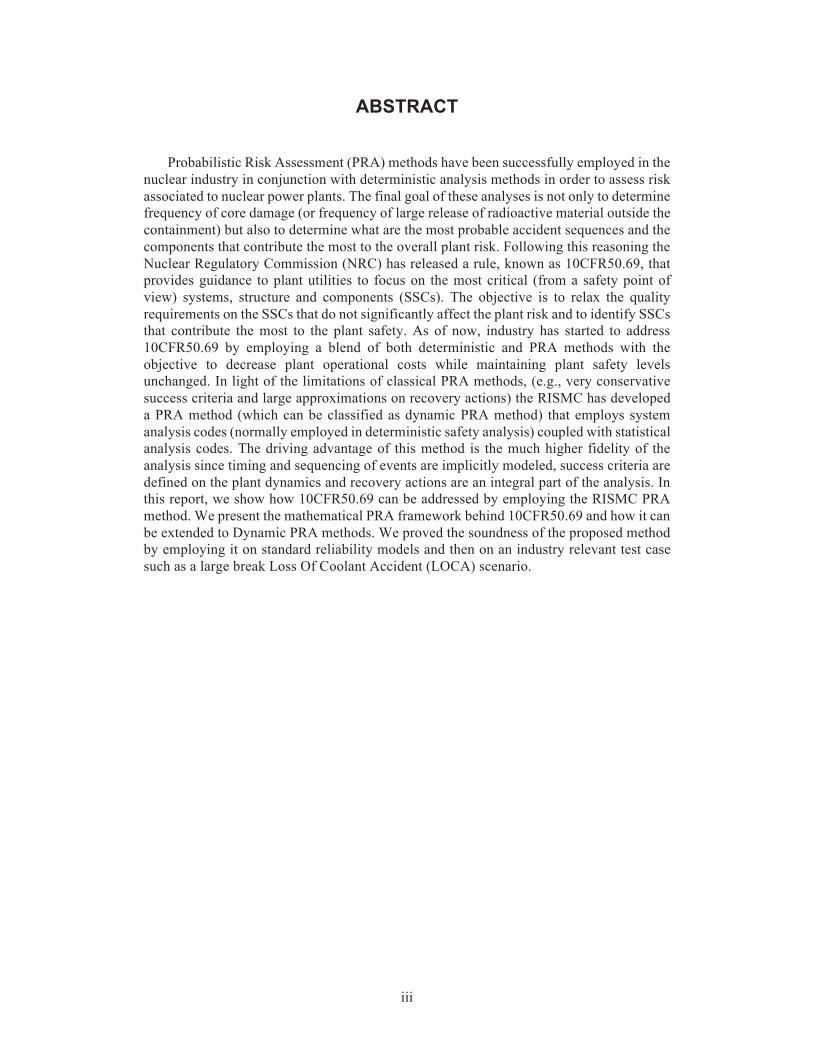
Probabilistic Risk Assessment (PRA) methods have been successfully employed in the nuclear industry in conjunction with deterministic analysis methods in order to assess risk associated to nuclear power plants. The final goal of these analyses is not only to determine frequency of core damage (or frequency of large release of radioactive material outside the containment) but also to determine what are the most probable accident sequences and the components that contribute the most to the overall plant risk. Following this reasoning the Nuclear Regulatory Commission (NRC) has released a rule, known as 10CFR50.69, that provides guidance to plant utilities to focus on the most critical (from a safety point of view) systems, structure and components (SSCs). The objective is to relax the quality requirements on the SSCs that do not significantly affect the plant risk and to identify SSCs that contribute the most to the plant safety. As of now, industry has started to address 10CFR50.69 by employing a blend of both deterministic and PRA methods with the objective to decrease plant operational costs while maintaining plant safety levels unchanged. In light of the limitations of classical PRA methods, (e.g., very conservative success criteria and large approximations on recovery actions) the RISMC has developed a PRA method (which can be classified as dynamic PRA method) that employs system analysis codes (normally employed in deterministic safety analysis) coupled with statistical analysis codes. The driving advantage of this method is the much higher fidelity of the analysis since timing and sequencing of events are implicitly modeled, success criteria are defined on the plant dynamics and recovery actions are an integral part of the analysis. In this report, we show how 10CFR50.69 can be addressed by employing the RISMC PRA method. We present the mathematical PRA framework behind 10CFR50.69 and how it can be extended to Dynamic PRA methods. We proved the soundness of the proposed method by employing it on standard reliability models and then on an industry relevant test case such as a large break Loss Of Coolant Accident (LOCA) scenario.
iv
ABSTRACT .................................................................................................................................... iii
FIGURES .......................................................................................................................................... v
TABLES ......................................................................................................................................... vi
ACRONYMS ................................................................................................................................. vii
1. Introduction ............................................................................................................................ 11.1 Overview of 10CFR50.69 ............................................................................................ 21.2 Summary of R&D Activities ....................................................................................... 3
2. The RISMC Approach ............................................................................................................ 5
3. Measuring Risk Importance ................................................................................................... 73.1 Classical PRA Importance Metrics .............................................................................. 73.2 Simulation-based PRA Importance Metrics ................................................................ 73.3 Potential Applications Within 10CFR50.69 .............................................................. 12
4. Application: PWR LB-LOCA .............................................................................................. 134.1 Results ........................................................................................................................ 14
5. Conclusions .......................................................................................................................... 185.1 Publications ................................................................................................................ 18
6. REFERENCES ..................................................................................................................... 19
APPENDIX A ................................................................................................................................. 21
APPENDIX B ................................................................................................................................. 22
v
Figure 1. Example of system analysis using a combination FTs and ETs. ....................................... 1
Figure 2. Categorization of SSCs according to NRC rule 10CFR50.69. .......................................... 3
Figure 3. Overview of the RISMC modeling approach. ................................................................... 5
Figure 4. Relationship between simulator physics code (H) and control logic (C). ......................... 6
Figure 5. Treatment of discrete (top) and continuous (bottom) stochastic variables for reliability purposes. ........................................................................................................................... 9
Figure 6. Plot of a hypothetical ........................................................................................ 10
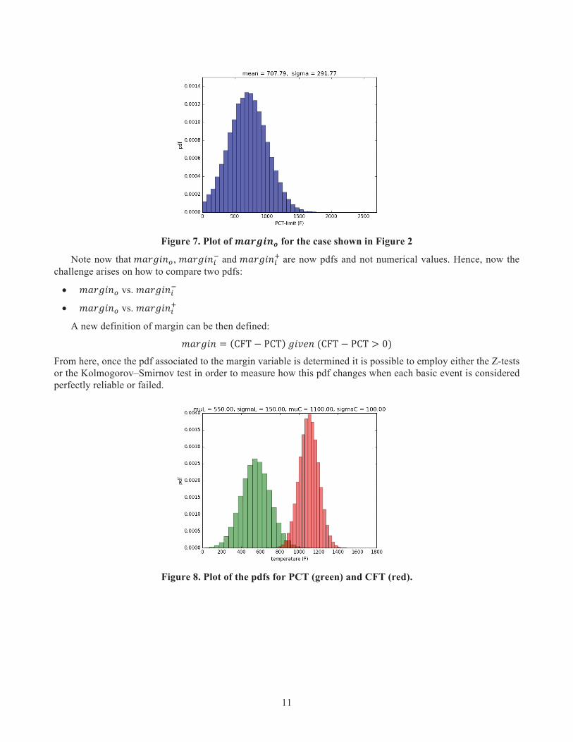
Figure 7. Plot of for the case shown in Figure 2 ............................................................. 11
Figure 8. Plot of the pdfs for PCT (green) and CFT (red). ............................................................. 11
Figure 9. Plot of the pdf of the variable (left) and plot of the pdf of the margin, i.e., (right). ..................................................................................................... 12
Figure 10. PWR scheme. ................................................................................................................ 13
Figure 11. PWR LB-LOCA analysis overview. ............................................................................. 14
Figure 12. Brach probability comparison. ...................................................................................... 15
Figure 13. Histogram of PCT for the simulation belonging to branch 4 (see Figure 12) ............... 15
Figure 14. Updated ET structure given RELAP5-3D/RAVEN analysis. ....................................... 16
Figure 15. LBLOCA DEGB cases. PCT (left), RPV level (right). ................................................. 17

vi
Table 1. LBLOCA DEGB results. .................................................................................................. 16
vii
ACC Accumulator system CD Core Damage CS Containment Spray DOE Department of Energy ECCS Emergency Core Cooling System EDG Emergency Diesel Generator EPRI Electric Power Research Institute ET Event-Tree FT Fault-Tree FV Fusel-Vessely INL Idaho National Laboratory LB-LOCA Large Break LOCA LOCA Loss Of Coolant Accident LPI Low Pressure Injection system LPR Low Pressure Recirculation system LWRS Light Water Reactor Sustainability MC Monte-Carlo NPP Nuclear Power Plant NRC Nuclear Regulatory Commission PCT Peak Clad Temperature PRA Probabilistic Risk Assessment PWR Pressurized Water Reactor pdf Probabilistic Distribution Function R&D Research and Development RAVEN Risk Analysis Virtual ENvironment RAW Risk Achievement Worth RIM Risk Importance Measure RRW Risk Reduction Worth RISC Risk Informed Safety Class RISMC Risk-Informed Safety Margin Characterization ROM Reduced Order Model RPV Reactor Pressure Vessel RRW Risk Reduction Worth RWST Reactor Water Storage Tank SG Steam Generator SI Safety Injection

viii
SR Safety Related SSCs Systems , Structures and Components
1
Safety and risk associated to nuclear power plants are typically measured by employing Probabilistic Risk Assessment (PRA) methods in conjunction with deterministic analysis methods. Deterministic methods employ system analysis codes (e.g., RELAP5 [1] or MELCOR [2]) in order to assure that plant safety systems can prevent Core Damage (CD) condition for a given set of accident conditions. PRA methods [3] employ static Boolean logic structures (Event Trees – FT – and Fault-Tree – FT –) in order to determine accident sequences that includes failure of System Structure and Components (SSCs) given a set of prescribed initiating events.
The goal of PRA methods is not only to determine frequency of CD (or frequency of large release of radioactive material outside the containment or early cancer fatalities) but also to determine what are the most probable accident sequences and the components that contribute the most to the overall plant risk.
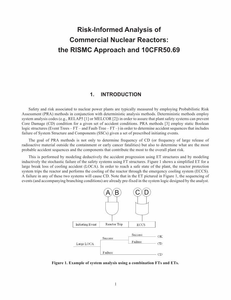
This is performed by modeling deductively the accident progression using ET structures and by modeling inductively the stochastic failure of the safety systems using FT structures. Figure 1 shows a simplified ET for a large break loss of cooling accident (LOCA). In order to reach a safe state of the plant, the reactor protection system trips the reactor and performs the cooling of the reactor through the emergency cooling system (ECCS). A failure in any of these two systems will cause CD. Note that in the ET pictured in Figure 1, the sequencing of events (and accompanying branching conditions) are already pre-fixed in the system logic designed by the analyst.
Figure 1. Example of system analysis using a combination FTs and ETs.
2
Branching probabilities associated to Reactor Trip and ECCS are determined using FTs: a combinations of logic gates (e.g., AND and OR gates) which connect basic events (i.e., A, B, C and D) to the Top Event (e.g., failure of ECCS). For the system pictured in Figure 1, the reactor trip system can fail if both events A and B occur (“AND” gate) while ECCS system fails if either events C or D occur (“OR” gate)
In light of the limitations of classical PRA methods (e.g., very conservative success criteria and large approximations on recovery actions) the RISMC project [4] has developed a PRA method (which can be classified as dynamic PRA method) that employs system analysis codes (normally employed in deterministic safety analysis) coupled with statistical analysis codes. The driving advantage of this method is the much higher fidelity of the analysis since timing and sequencing of events are implicitly modeled, success criteria are defined on the plant dynamics and recovery actions are integral part of the analysis.
In early 2000, the Nuclear Regulatory Commission (NRC) released a rule, known as 10CFR50.69, that provides guidance to plant utilities and operators to focus on the most critical (from a safety point of view) systems, structures and components (SSCs). The objective is to relax the quality requirements (and, thus, decrease procurement costs) on the SSCs that do no significantly affect the plant risk and to identify SSCs that actually contribute the most to the plant safety. As of now, industry has started to address 10CFR50.69 by employing a blend of both deterministic and PRA methods with the objective to decrease plant operational costs while maintaining plant safety levels unchanged.
The essential step behind 10CFR50.69 is to measure risk importance of SSCs [5]: this is usually performed using classical Risk Importance Measures (RIMs) such as Risk Achievement Worth (RAW) and Fusel-Vessely (FV) applied to the data generated ET-FT methods (i.e., cut sets).
In this report we show how 10CFR50.69 can be addressed by employing the RISMC PRA method. Firstly, we present the mathematical PRA framework behind measuring risk importance of SSCs and how it can be extended to Dynamic PRA methods. We proved the soundness of the proposed method by employing it on standard reliability models and then on an industry relevant test case such as a Large Break Loss Of Coolant Accident (LOCA) scenario.
In early 2000s, the US Nuclear Regulatory Commission (NRC) released the 10CFR50.69 [6] rule which contains categorization requirements for plant SSCs supported by a regulatory guide. Additionally, the rule contains a new treatment requirements that applies to SSCs based on their associated risk-informed safety class (RISC) categorization. This rule has the benefit of grouping and integrating all the risk-informed requirements into one single rule.
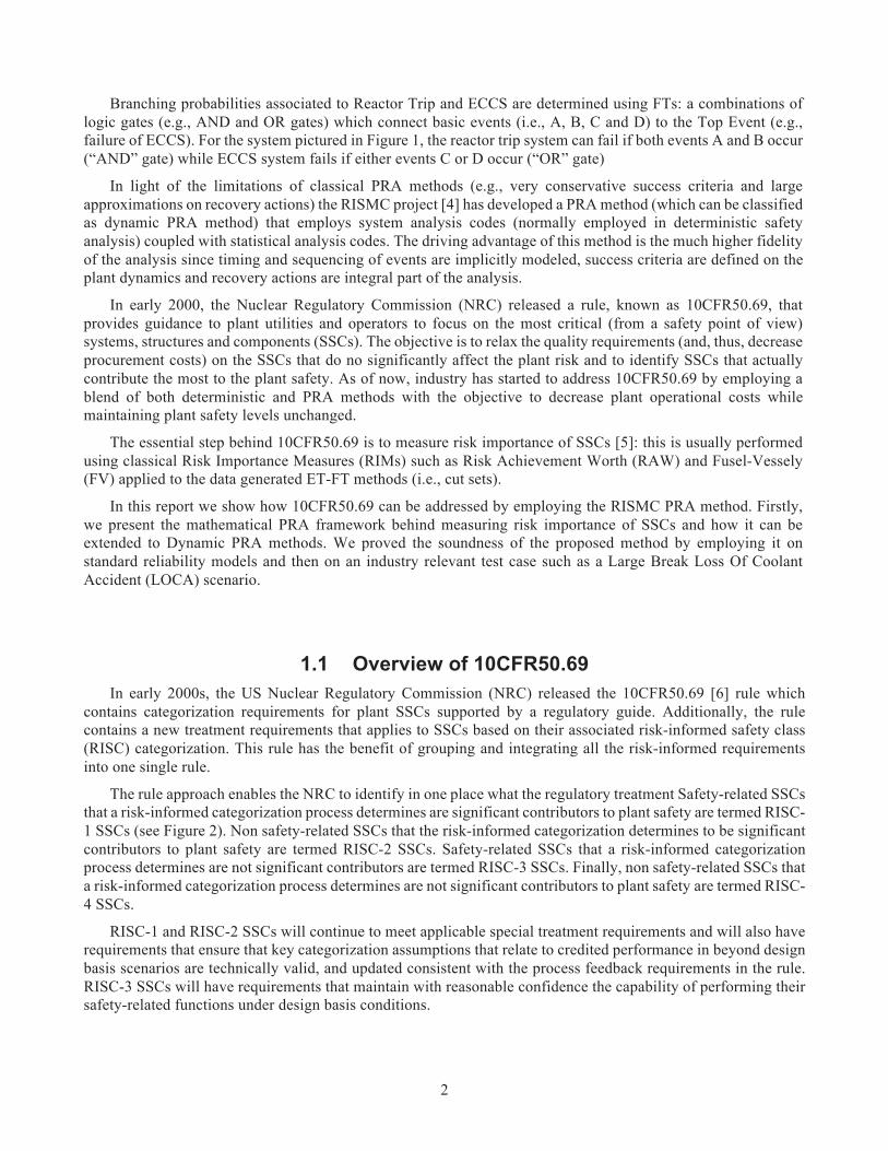
The rule approach enables the NRC to identify in one place what the regulatory treatment Safety-related SSCs that a risk-informed categorization process determines are significant contributors to plant safety are termed RISC-1 SSCs (see Figure 2). Non safety-related SSCs that the risk-informed categorization determines to be significant contributors to plant safety are termed RISC-2 SSCs. Safety-related SSCs that a risk-informed categorization process determines are not significant contributors are termed RISC-3 SSCs. Finally, non safety-related SSCs that a risk-informed categorization process determines are not significant contributors to plant safety are termed RISC-4 SSCs.
RISC-1 and RISC-2 SSCs will continue to meet applicable special treatment requirements and will also have requirements that ensure that key categorization assumptions that relate to credited performance in beyond design basis scenarios are technically valid, and updated consistent with the process feedback requirements in the rule. RISC-3 SSCs will have requirements that maintain with reasonable confidence the capability of performing their safety-related functions under design basis conditions.
3
RISC-4 SSCs will be removed from any applicable special treatment requirements and have no additional requirements imposed by 10CFR50.69 rule (recognizing that any technical/functional requirements continue to apply unless they are changed via the normal design change process including 10CFR50.69 rule).
As part of the “Delivering the Nuclear Promise”, the Nuclear Energy Institute (NEI) in collaboration with Electric Power Research Institute (EPRI) started a set of operational activities to assist the nuclear industry with the goals of:
• Maintain Operational record: safety remains an essential priority, advanced reliability and resilience of plants
• Increase value: clean energy benefits, R&D improvements
• Improve efficiency: reduced operation costs, maintain/increase capacity factor
The last goal (i.e., the reduction of operational costs) is being addressed by extensively employing the 10CFR50.69 rule for a large number of plant systems.
Figure 2. Categorization of SSCs according to NRC rule 10CFR50.69.
During FY17, as part of this R&D project, we have performed the following activities in order to address 10CFR50.69 using the RISMC approach:
1. Development of RIMs for any data generated by simulation-based (i.e., dynamic) PRA method such as Monte-Carlo [7] or Dynamic Event Trees (DETs) [8]
2. Implementation of these RIMs as integral part of the RAVEN statistical framework
3. Extension of these RIMs on a time dependent domain which can be used as part of risk-monitoring tools

4
4. Validation of the proposed RIMs against analytical test cases and against classical PRA tools such as SAPHIRE
5. Performed a full simulation based PRA analysis for an industry level test case such as PWR LB-LOCA
6. Comparison of the analysis between RAVEN-RELAP5 and SAPHIRE on the PWR LB-LOCA test case
7. Development of new margin-centric RIMs that incorporate in the assessment the intrinsic dynamic behavior of accident progression
5
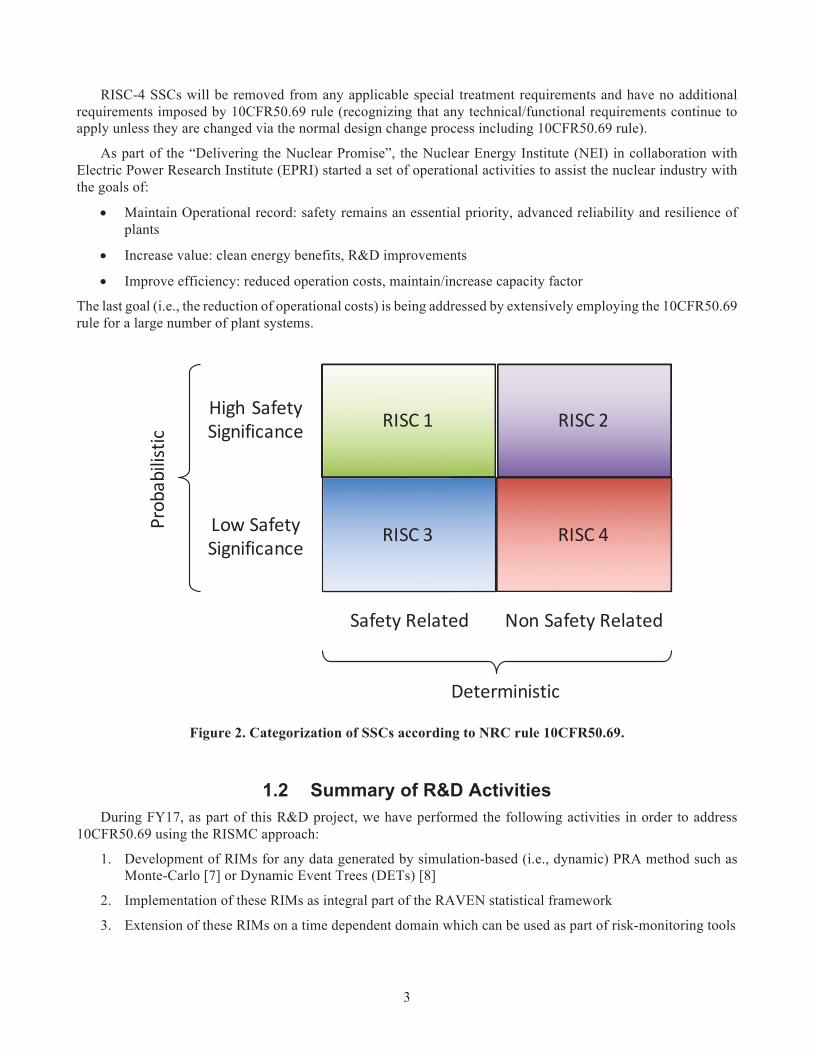
The RISMC approach employs both deterministic and stochastic methods in a single analysis framework (see Figure 3). In the deterministic method set we include:
• Modeling of the thermal-hydraulic behavior of the plant [9]
• Modeling of external events such as flooding [10]
• Modeling of the operator responses to the accident scenario [11]
Note that deterministic modeling of the plant or external events can be performed by employing specific simulator codes but also surrogate models [12], known as reduced order models (ROM). ROMs would be employed in order to decrease the high computational costs of codes. In addition, multi-fidelity codes can be employed to model the same system; the idea is to switch from low-fidelity to high-fidelity code when higher accuracy is needed (e.g., use low-fidelity codes for steady-state conditions and high-fidelity code for transient conditions)
In the stochastic modelling we include all stochastic parameters that are of interest in the PRA analysis such as:
• Uncertain parameters
• Stochastic failure of system/components
Figure 3. Overview of the RISMC modeling approach.
The RISMC approach heavily relies on multi-physics system simulator codes (e.g., RELAP5-3D [1]) coupled with stochastic analysis tools (e.g., RAVEN [13,14]). From a PRA point of view, a simulation run can be described by using two sets of variables:
• represents the status of components and systems of the simulator (e.g., status of emergency core cooling system, AC system)
Parameters Distribution
Wave height (m) Exponential
Wave impact time (h) Uniform
Diesel recovery time (h) Weibull
Off-site grid recovery timea (h) Lognormal
Off-site grid recovery timeb (h) Lognormal
Batteries failure time (h) Triangular
Batteries recovery time (h) Lognormal recccccoocovoovovovovvvovovcccovovovovcoovovccoccovovccccoc tery te tery teery teery tery tery ti (i (i (ime (ime (ime (ime (ime (h)h)h)h)h)h)h)h) LLLLognoLognoLognoLognoLogno lllrmalrmalrmalrmalrmal
6
• represents the temporal evolution of a simulated accident scenario, i.e., represents a single simulation run. Each element of can be for example the values of temperature or pressure in a specific node of the simulator nodalization.
From a mathematical point of view, a single simulator run can be represented as a single trajectory in the phase space. The evolution of such a trajectory in the phase space can be described as follows:
(1)
where:
• is the actual simulator code that describes how evolves in time
• is the operator which describes how evolves in time, i.e., the status of components and systems at each time step
• is the set of stochastic parameters
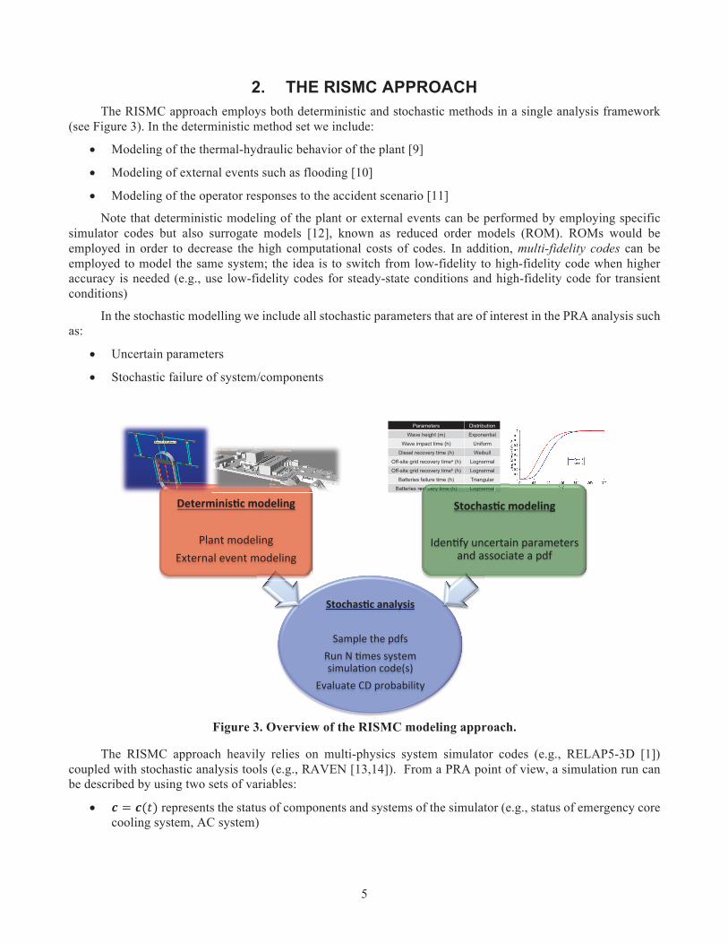
Starting from the system located in an initial state, , and the set of stochastic parameter values (which are generally generated through a stochastic sampling process), the simulator determines at each time step the temporal evolution of . At the same time, the system control logic1 determines the status of the system and components . The coupling between these two sets of variables is shown in Figure 4.
Figure 4. Relationship between simulator physics code (H) and control logic (C).
By using the RISMC approach, the PRA analysis is performed by [15]:
1. Associating a probabilistic distribution function (pdf) to the set of stochastic parameters (e.g., timing of events)
2. Performing stochastic sampling of the pdfs defined in Step 1
3. Performing a simulation run given sampled in Step 2, i.e., solve the system of equations (1)
4. Repeating Steps 2 and 3 M times and evaluating user defined stochastic parameters such as CD probability ( ).
The goal of RIM analysis is to measure risk importance of the set of stochastic parameters . The analysis presented in this report focuses on how RIMs can be extended to Dynamic PRA data.
1 Which is usually an integral part of the system simulator
Θ(t) c(t)
H
C
Θ(0) s
7
The value of a PRA analysis is not limited to the determination of the risk associated to a nuclear power plant (through the determination of CD or LERF probability) but, more importantly, it provides insights about which components/systems impact the most the plant risk and which ones are the most safety relevant (i.e., they assure plant basic safety functions).
These insights can be generated by defining a set of metrics that measure the risk importance of system/components. Typically, in classical PRA methods, the set of metrics are determined by evaluating CD probability assuming the component failed or perfectly reliable (see Section 3.1).
In ET-FT based PRA methods, for any basic event, the most used RIMs measures are: Risk Achievement Worth (RAW), Risk Reduction Worth (RRW), Birnbaum (B) and Fussell-Vesely (FV) [5,16]. All these RIMs are calculated by determining three values based on core damage frequency (CDF):
• : nominal CDF
• : CDF for basic event i assuming perfectly reliable
• : CDF for basic event i assuming it has failed
Once these three values are determined, then the RIMs are calculated [5] as follows for each basic event i:
(1)
(2)
(3)
(4)
Note the four RIMs listed above is not exhaustive; in literature, it is possible to find additional RIMs such as the Differential Importance Measure (DIM) [17]. Since, the scope of this paper is limited to risk-informed application of 10CFR50.69, we focused this report only on the four RIMs listed above.
In a Dynamic PRA environment, is obtained (e.g., through Monte-Carlo sampling) by:
• Running simulations (e.g., RELAP5-3D runs)
• Counting the number of simulations that lead to core damage (CD) condition
• Calculating
Note that while basic events in classical PRA are mainly Boolean, in a Dynamic PRA environment the sample parameters can be, not only Boolean, but more often continuous. In this work we assume that basic events in a classical PRA framework coincide with the stochastic parameters in a RISMC framework.
As an example, let us consider two basic events:
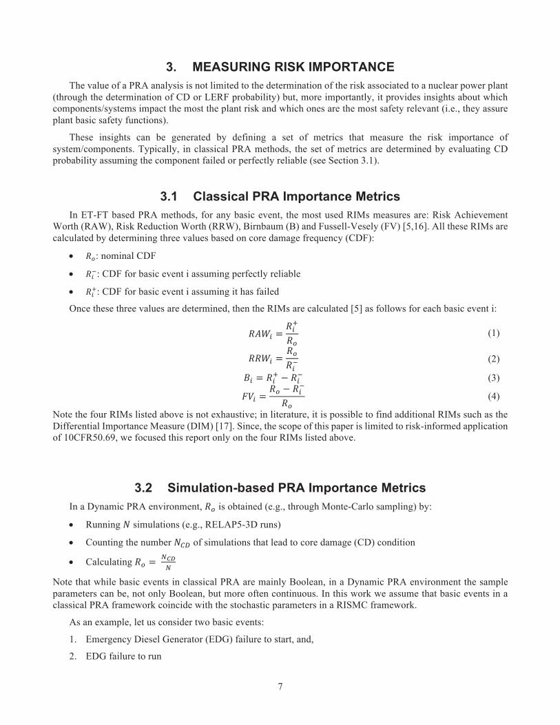
1. Emergency Diesel Generator (EDG) failure to start, and,
2. EDG failure to run
8
In classical PRA analysis, a probability value is associated to both basic events. On the other side, in a Dynamic PRA framework, a Bernoulli distribution could be associated to the first basic event and a continuous distribution (e.g., exponential distribution) could be associated to the second basic event.
At this point a challenge arises: the determination of and for each sampled parameter; two possible approaches can be followed2:
1. Perform a Dynamic PRA for and for each and
2. Determine an approximated value of and from the simulation runs generated to calculate
Regarding Approach 1, given the computational costs of each Dynamic PRA, it is unfeasible to determine and for each sampled parameter. In fact, if we consider sample parameters (i.e., S basic events), then the risk importance analysis would require Dynamic PRA analyses.
Regarding Approach 2, a method (implemented in RAVEN as an internal post-processor) was developed and it is here presented. This method requires an input from the user:
• Range, , of the variable that can be associated to “basic event with component perfectly reliable”
• Range, , of the variable that can be associated to “basic event in a failed status”
Given this kind of information, it is possible to calculate and as follows3:
(6)
(7)
(8)
Note that this approach has an issue related to the choices of and . Depending on their values, and might change accordingly. In addition, the statistical error associated to the estimates of and also changes.
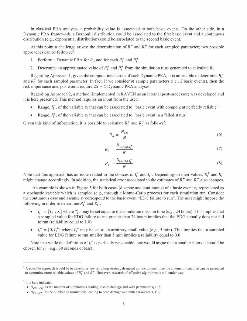
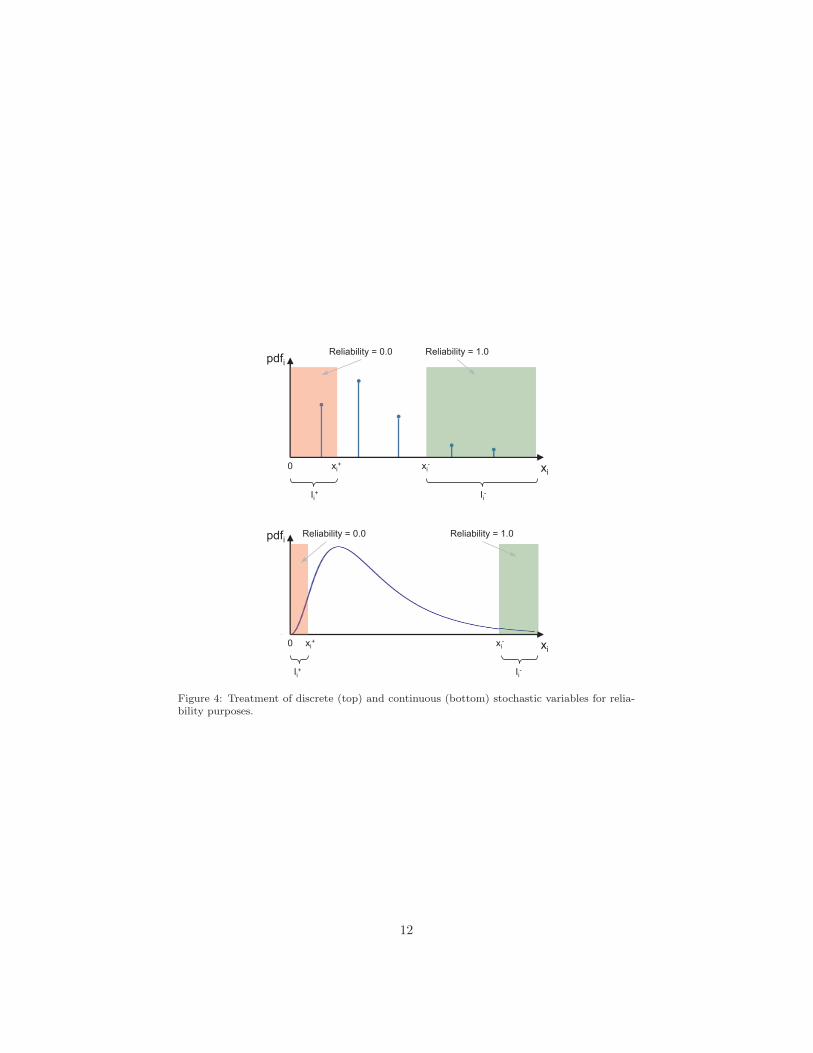
An example is shown in Figure 5 for both cases (discrete and continuous) of a basic event represented as a stochastic variable which is sampled (e.g., through a Monte-Carlo process) for each simulation run. Consider the continuous case and assume correspond to the basic event “EDG failure to run”. The user might impose the following in order to determine and :
• where may be set equal to the simulation mission time (e.g., 24 hours). This implies that a sampled value for EDG failure to run greater than 24 hours implies that the EDG actually does not fail to run (reliability equal to 1.0)
• where may be set to an arbitrary small value (e.g., 5 min). This implies that a sampled value for EDG failure to run smaller than 5 min implies a reliability equal to 0.0
Note that while the definition of is perfectly reasonable, one would argue that a smaller interval should be chosen for (e.g., 30 seconds or less).
2 A possible approach would be to develop a new sampling strategy designed ad-hoc to maximize the amount of data that can be generated
to determine more reliable values of and . However, research of effective algorithms is still under way. 3 It is here indicated: • as the number of simulations leading to core damage and with parameter • as the number of simulations leading to core damage and with parameter
9
Recall that ideally, a value of should be theoretically chosen (and not an interval); however, given the nature of the distribution this is not allowed. Given the nature of the problem, we are bound to choose an interval :
• A small interval in the neighbor of would lead to a value of close to the theoretical one. However, the number of actual sampled values falling in would be very small, i.e., large stochastic error.
• A large interval in the neighbor of would lead to a value of far from the theoretical one. However, the number of actual sampled values falling in would be very high, i.e., small stochastic error.
A solution to the large statistical error associated to a very small interval can be solved by employing different sampling algorithms other than the classical Monte-Carlo one.
Figure 5. Treatment of discrete (top) and continuous (bottom) stochastic variables for reliability
purposes.
As an example, a better resolution of the final value for can be achieved by sampling uniformly the range of variability of and associating an importance weight to each sample. At this point the counting variable is weighted by the weight of each sample. By sampling uniformly the range of variability of , the number of samples in the interval would be significantly higher.
Note that the RIMs described so far are limited to a binary logic of the outcome variable (e.g., OK vs. CD). Dynamic PRA approaches typically generate a continuous value of the outcome variables (e.g., Peak Clad Temperature - PCT). In our application (see previous sections) we typically convert PCT to a discrete one as follows:
• : outcome = CD
pdfi
xi 0 xi+ xi
-
Ii+ Ii-
pdfi
xi 0 xi+ xi
-
Ii+ Ii-
Reliability = 1.0 Reliability = 0.0
Reliability = 1.0 Reliability = 0.0
10
• : outcome = OK
Given the different structure of the approach used in this paper to solve a PRA problem (i.e., Dynamic instead of classical PRA), the reader might think that a different set of RIMs should/could be developed in order to capture the nature of the problem solved using Dynamic PRA.
As a starting point, it would be worth investigating the nominal probabilistic distribution (pdf) of PCT with the one obtained when reliability of each basic event (sampled parameter) is 0.0 or 1.0. So now we can indicate:
1. : nominal pdf of PCT
2. : pdf of PCT associated to basic event assuming basic event is perfectly reliable
3. : pdf of PCT associated to basic event assuming basic event has failed
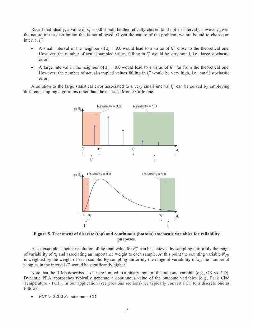
An example is shown below for a hypothetical case where obtained is indicated using an histogram while the limit value for PCT is shown using the red line passing at 2200 F.
In order to make a connection to what has been presented in the previous section, note that by looking at Figure 6:
As part of the RISMC analysis, the user might want to supplement the results obtained in the previous section with the information associated to a more effective margin analysis.
In particular, of interest for RISMC applications is (see Figure 7) the concept of margin:
given
Figure 6. Plot of a hypothetical
Using the same philosophy indicated in the previous section for classical RIMs, we want to determine:
1. : pdf of the variable given that
2. : pdf of the variable given that for basic event assuming it is perfectly reliable
3. : pdf of the variable given that for basic event when its assumed to be failed
11
Figure 7. Plot of for the case shown in Figure 2
Note now that , and are now pdfs and not numerical values. Hence, now the challenge arises on how to compare two pdfs:
• vs.
• vs.
A new definition of margin can be then defined:
From here, once the pdf associated to the margin variable is determined it is possible to employ either the Z-tests or the Kolmogorov–Smirnov test in order to measure how this pdf changes when each basic event is considered perfectly reliable or failed.
Figure 8. Plot of the pdfs for PCT (green) and CFT (red).
12
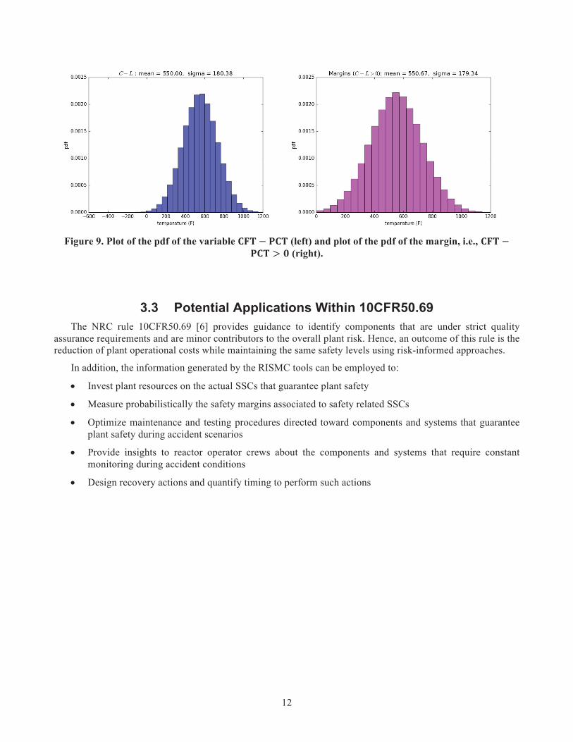
Figure 9. Plot of the pdf of the variable (left) and plot of the pdf of the margin, i.e.,
(right).
The NRC rule 10CFR50.69 [6] provides guidance to identify components that are under strict quality assurance requirements and are minor contributors to the overall plant risk. Hence, an outcome of this rule is the reduction of plant operational costs while maintaining the same safety levels using risk-informed approaches.
In addition, the information generated by the RISMC tools can be employed to:
• Invest plant resources on the actual SSCs that guarantee plant safety
• Measure probabilistically the safety margins associated to safety related SSCs
• Optimize maintenance and testing procedures directed toward components and systems that guarantee plant safety during accident scenarios
• Provide insights to reactor operator crews about the components and systems that require constant monitoring during accident conditions
• Design recovery actions and quantify timing to perform such actions
13
In order to test the methods here proposed we have identified several analytical test cases based on classical reliability configurations (e.g., series/parallel, components in stand-by, K-out-of-N) and we have also developed additional test cases using industry PRA codes such SAPHIRE. For all cases, the obtained results were matching the analytical ones within the statistical error boundaries.
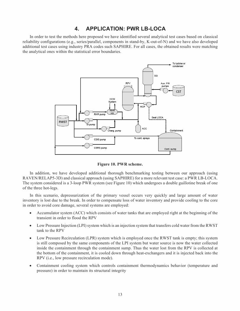
Figure 10. PWR scheme.
In addition, we have developed additional thorough benchmarking testing between our approach (using RAVEN/RELAP5-3D) and classical approach (using SAPHIRE) for a more relevant test case: a PWR LB-LOCA. The system considered is a 3-loop PWR system (see Figure 10) which undergoes a double guillotine break of one of the three hot-legs.
In this scenario, depressurization of the primary vessel occurs very quickly and large amount of water inventory is lost due to the break. In order to compensate loss of water inventory and provide cooling to the core in order to avoid core damage, several systems are employed:
• Accumulator system (ACC) which consists of water tanks that are employed right at the beginning of the transient in order to flood the RPV
• Low Pressure Injection (LPI) system which is an injection system that transfers cold water from the RWST tank to the RPV
• Low Pressure Recirculation (LPR) system which is employed once the RWST tank is empty; this system is still composed by the same components of the LPI system but water source is now the water collected inside the containment through the containment sump. Thus the water lost from the RPV is collected at the bottom of the containment, it is cooled down through heat-exchangers and it is injected back into the RPV (i.e., low pressure recirculation mode).
• Containment cooling system which controls containment thermodynamics behavior (temperature and pressure) in order to maintain its structural integrity
14
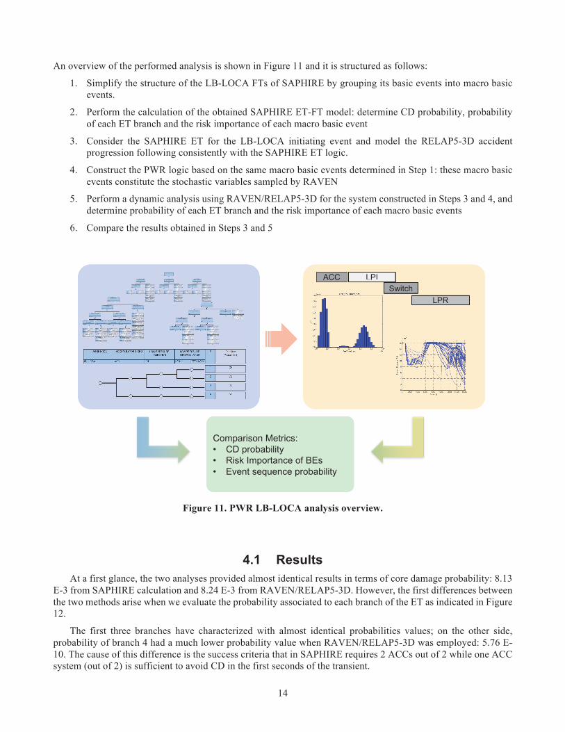
An overview of the performed analysis is shown in Figure 11 and it is structured as follows:
1. Simplify the structure of the LB-LOCA FTs of SAPHIRE by grouping its basic events into macro basic events.
2. Perform the calculation of the obtained SAPHIRE ET-FT model: determine CD probability, probability of each ET branch and the risk importance of each macro basic event
3. Consider the SAPHIRE ET for the LB-LOCA initiating event and model the RELAP5-3D accident progression following consistently with the SAPHIRE ET logic.
4. Construct the PWR logic based on the same macro basic events determined in Step 1: these macro basic events constitute the stochastic variables sampled by RAVEN
5. Perform a dynamic analysis using RAVEN/RELAP5-3D for the system constructed in Steps 3 and 4, and determine probability of each ET branch and the risk importance of each macro basic events
6. Compare the results obtained in Steps 3 and 5
Figure 11. PWR LB-LOCA analysis overview.
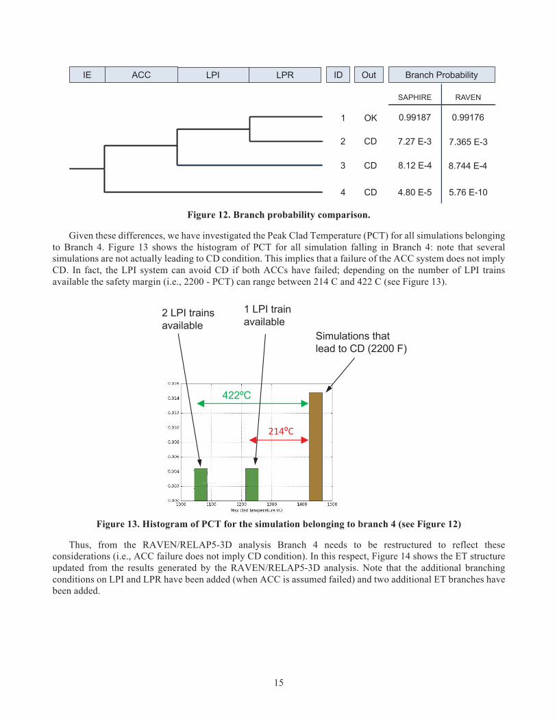
At a first glance, the two analyses provided almost identical results in terms of core damage probability: 8.13 E-3 from SAPHIRE calculation and 8.24 E-3 from RAVEN/RELAP5-3D. However, the first differences betweenthe two methods arise when we evaluate the probability associated to each branch of the ET as indicated in Figure 12.
The first three branches have characterized with almost identical probabilities values; on the other side, probability of branch 4 had a much lower probability value when RAVEN/RELAP5-3D was employed: 5.76 E-10. The cause of this difference is the success criteria that in SAPHIRE requires 2 ACCs out of 2 while one ACC system (out of 2) is sufficient to avoid CD in the first seconds of the transient.
15
Figure 12. Branch probability comparison.
Given these differences, we have investigated the Peak Clad Temperature (PCT) for all simulations belonging to Branch 4. Figure 13 shows the histogram of PCT for all simulation falling in Branch 4: note that several simulations are not actually leading to CD condition. This implies that a failure of the ACC system does not imply CD. In fact, the LPI system can avoid CD if both ACCs have failed; depending on the number of LPI trains available the safety margin (i.e., 2200 - PCT) can range between 214 C and 422 C (see Figure 13).
Figure 13. Histogram of PCT for the simulation belonging to branch 4 (see Figure 12)
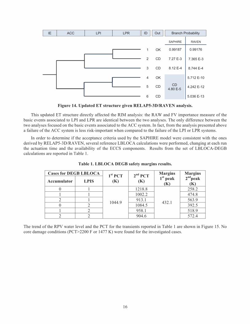
Thus, from the RAVEN/RELAP5-3D analysis Branch 4 needs to be restructured to reflect these considerations (i.e., ACC failure does not imply CD condition). In this respect, Figure 14 shows the ET structure updated from the results generated by the RAVEN/RELAP5-3D analysis. Note that the additional branching conditions on LPI and LPR have been added (when ACC is assumed failed) and two additional ET branches have been added.
16
Figure 14. Updated ET structure given RELAP5-3D/RAVEN analysis.
This updated ET structure directly affected the RIM analysis: the RAW and FV importance measure of the basic events associated to LPI and LPR are identical between the two analyses. The only difference between the two analyses focused on the basic events associated to the ACC system. In fact, from the analysis presented above a failure of the ACC system is less risk-important when compared to the failure of the LPI or LPR systems.
In order to determine if the acceptance criteria used by the SAPHIRE model were consistent with the ones derived by RELAP5-3D/RAVEN, several reference LBLOCA calculations were performed, changing at each run the actuation time and the availability of the ECCS components. Results from the set of LBLOCA-DEGB calculations are reported in Table 1.
Table 1. LBLOCA DEGB safety margins results.
Cases for DEGB LBLOCA 1st PCT (K)
2nd PCT (K)
Margins 1st peak
(K)
Margins 2ndpeak
(K) Accumulator LPIS
0 1
1044.9
1218.8
432.1
258.2 1 1 1002.2 474.8 2 1 913.1 563.9 0 2 1084.5 392.5 1 2 958.1 518.9 2 2 904.6 572.4
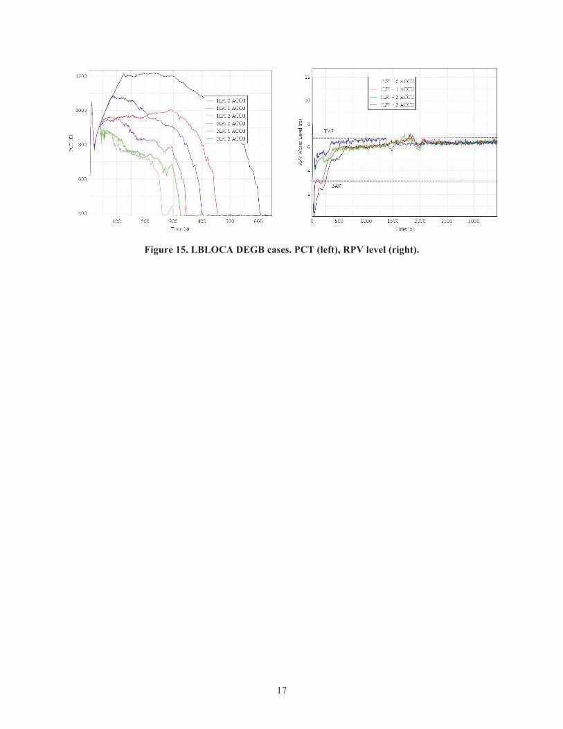
The trend of the RPV water level and the PCT for the transients reported in Table 1 are shown in Figure 15. No core damage conditions (PCT>2200 F or 1477 K) were found for the investigated cases.
17
Figure 15. LBLOCA DEGB cases. PCT (left), RPV level (right).
18
In this report we have developed a series of risk-informed methods which can be employed to measure risk-importance of system/components using simulation-based PRA methods. The design/development of these methods has been such that they are compatible with risk-importance measures developed for classical PRA methods. A series of analytical tests have been performed in order to prove the validity of such methods using classical reliability models.
We have performed an exhaustive PRA analysis of a PWR system for LLOCA initiating event using RAVEN coupled with RELAP5-3D and compared this analysis with the ones performed by employing classical PRA tools such as SAPHIRE. The comparison of the two sets of results highlighted the limitations of classical PRA methods when employed to analyze complex system such nuclear systems.
The analysis shows how the RISMC approach can be identified as an integrated deterministic and PRA method. Success criteria and timing/sequencing of events are implicitly modeled in the system simulator while stochastic model of systems/components are part of the sampling strategy.
This report can be considered a first step toward addressing the NRC rule 10CFR50.69. The categorization step that is part of the 10CFR50.69 process can in fact be performed by employing the methods presented in this report. Since the analysis performed using the RISMC approach is compatible with classical PRA methods, 10CFR50.69 can be performed by employing both classical and RISMC methods depending on the initiating event.
During FY17 the following publications were developed:
• Journal papers (see Appendices A and B):
o D. Mandelli, Z. Ma, C. Parisi, D. Maljovec, A. Alfonsi, C. Smith, “Measuring Risk-Importance in a Simulation-Based PRA Framework - Part I: Mathematical Framework”, Draft for Reliability Engineering and System Safety.
o D. Mandelli, C. Parisi, Z. Ma, D. Maljovec, A. Alfonsi, C. Smith, “Measuring Risk-Importance in a Simulation-Based PRA Framework - Part II: Comparison Between Simulation-Based and Classical PRA Methods”, Draft for Reliability Engineering and System Safety.
• Conference papers:
o D. Mandelli, Z. Ma, C. Parisi, A. Alfonsi, C. Smith, “Measuring Risk Importance in a Dynamic PRA Framework,” Proceedings for the Probabilistic Safety Assessment Conference PSA2017, American Nuclear Society (2017).
o D. Mandelli, A. Alfonsi, C. Smith, “Risk Monitoring Capabilities from Dynamic PRA Data,” Proceedings for the ANS Winter Meeting, American Nuclear Society (2017).
19
[1] RELAP5-3D Code Development Team, RELAP5-3D Code Manual (2005).
[2] R. O. Gauntt, “MELCOR Computer Code Manual, Version 1.8.5”, Vol. 2, Rev. 2. Sandia National Laboratories, NUREG/CR-6119.
[3] U.S. Nuclear Regulatory Commission, “Severe accident risks: an assessment for five U.S. nuclear power plants Final Summary Report”, NUREG-1150, Washington DC (1990).
[4] C. Smith, C. Rabiti, And R. Martineau, “Risk Informed Safety Margins Characterization (RISMC) Pathway Technical Program Plan”, Idaho National Laboratory technical report: INL/EXT-11-22977 (2011).
[5] W. Vesely et al., “Measures of risk importance and their applications”, NUREC/CR-3385 (1983).
[6] 10CFR50.69, Risk-Informed Categorization and Treatment of Structures, Systems and Components for Nuclear Power Reactors, Office of the Federal Register, National Archives and Records Administration, U.S. Government Printing Office, Washington, DC.
[7] E. Zio, M. Marseguerra, J. Devooght, And P. Labeau, “A concept paper on dynamic reliability via Monte Carlo simulation,” in Mathematics and Computers in Simulation, pp. 47-71 (1998).
[8] B. Rutt, U. Catalyurek, A. Hakobyan, K. Metzroth, T. Aldemir, R. Denning, S. Dunagan, And D. Kunsman, “Distributed dynamic event tree generation for reliability and risk assessment,” in Challenges of Large Applications in Distributed Environments, pp. 61-70, IEEE (2006).
[9] D. Mandelli, Z. Ma, And C. Smith, “Comparison of a traditional probabilistic risk assessment approach with advanced safety analysis,” in Proceeding of American Nuclear Society (2014).
[10] D. Mandelli, S. Prescott, C. Smith, A. Alfonsi, C. Rabiti, J. Cogliati, R. Kinoshita, “Modeling of a Flooding Induced Station Blackout for a Pressurized Water Reactor Using the RISMC Toolkit,” in ANS PSA 2015 International Topical Meeting on Probabilistic Safety Assessment and Analysis Columbia, SC, on CD-ROM, American Nuclear Society, LaGrange Park, IL, 2015.
[11] R. L. Boring, R. Benish Shirley, J. C. Joe, D, Mandelli, And C. Smith, “Simulation and Non-Simulation Based Human Reliability Analysis Approaches”, Idaho National Laboratory technical report: INL/EXT-14-33903 (2014).
[12] H. S. Abdel-Khalik, Y. Bang, J. M. Hite, C. B. Kennedy, C. Wang, “Reduced Order Modeling For Nonlinear Multi-Component Models,” International Journal on Uncertainty Quantification, 2 - 4, pp. 341-361 (2012).
[13] A. Alfonsi, C. Rabiti, D. Mandelli, J. Cogliati, R. Kinoshita, And A. Naviglio, “RAVEN and Dynamic Probabilistic Risk Assessment: Software Overview,” in Proceedings of European Safety and Reliability Conference ESREL (2014).
[14] C. Rabiti, A. Alfonsi, J. Cogliati, D. Mandelli, R. Kinoshita, RAVEN, a new software for dynamic risk analysis, in: Proceedings of the Probabilistic Safety Assessment and Management (PSAM) 12, 2014.
[15] D. Mandelli, C. Smith, T. Riley, J. Nielsen, A. Alfonsi, J. Cogliati, C. Rabiti, J. Schroeder, BWR station blackout: A RISMC analysis using RAVEN and RELAP5-3D, Nuclear Technology 193 (2016) 161{174.
[16] K. Fleming, “Developing useful insights and avoiding misleading conclusions from risk importance measures in PSA application”, Proceedings of PSA96, ANS (1996).
[17] E. Borgonovo, G. Apostolakis, “A new importance measure for risk-informed decision making”, Reliability Engineering and System Safety, 72, pp. 193-212 (2011)

20
[18] 10CFR50.69 SSC Categorization Guideline, Nuclear Energy Institute, Washington, DC, December 2005, NEI-00-04.

21
D. Mandelli, Z. Ma, C. Parisi, D. Maljovec, A. Alfonsi, C. Smith, “Measuring Risk-Importance in a Simulation-Based PRA Framework - Part I: Mathematical Framework”, Draft for Reliability Engineering and System Safety.
Measuring Risk-Importance in a Simulation-BasedPRA Framework - Part I: Mathematical Framework
D. Mandelli, Z. Ma, C. Parisi, D. Maljovec, A. Alfonsi, C. Smith
Idaho National Laboratory (INL), 2525 Fremont Ave, 83402 Idaho Falls (ID), USA
Abstract
Risk importance measures are indexes that are used to rank systems, structuresand components (SSCs) using risk-informed methods. The most used/knownmeasures are: Risk Reduction Worth (RRW), Risk Achievement Worth (RAW),Birnbaum (B) and Fussell-Vesely (FV). Once obtained from classical Proba-bilistic Risk Analysis (PRA) analyses, these risk measures can be effectivelyemployed to relatively rank component importance. In contrast to classicalPRA methods, Dynamic PRA methods couple stochastic models with safetyanalysis codes to determine risk associate to complex systems such as nuclearplants. Compared to classical PRA methods, simulation-based approaches canevaluate with higher resolution the safety impact of timing and sequencing ofevents on the accident progression. The objective of this paper is to presenta series of methods that can be employed to measure risk importance of com-ponents which are part of complex systems such as nuclear power plants. Thefirst set of measures are directly derived from classical risk importance measures(e.g., RRW, RAW, B and FV) and that can be employed to any Dynamic PRAanalysis. In addition, we provide a set of risk importance measures that capturethe dynamic nature of the problem and provide insight related to plant safetymargins.
Keywords: Importance Measures, Dynamic PRA, Probabilistic RiskAssessment
1. Introduction
Risk Importance Measures (RIMs) [1] are indexes that are used to ranksystems, structures and components (SSCs) based on their contribution to theoverall risk. The most used measures [2] are: Risk Reduction Worth (RRW),Risk Achievement Worth (RAW), Birnbaum (B) and Fussell-Vesely (FV).5
Typically, this ranking is performed in a classical PRA framework, whererisk is determined by considering probability associated to the minimal cut setsgenerated by static Boolean logic structures [3] (e.g., Event-Trees, Fault-Trees).In a classical PRA analysis, each SSC is represented by a set of basic events; as
Preprint submitted to Reliability Engineering & System Safety September 29, 2017
an example emergency diesel generators can be represented by two basic events:10
failure to start and failure to run.The risk measures associated to each basic event are calculated from the
generated cut-sets by determining:
• The nominal risk
• The increased risk assuming basic event failed15
• The reduced risk assuming basic event perfectly reliable
In this context, the Nuclear Regulatory Commission (NRC) has issued the10CFR50.69 document [4] allowing plant owners to perform a risk-informedcategorization and treatment of SSCs in order to reduce operating and mainte-nance costs while preserving acceptable risk levels. The described categorization20
is based on a set of risk importance measures obtained from the plant classicPRA models.
In contrast to classical PRA methods, Dynamic PRA methods [5] couplestochastic models (e.g., RAVEN [6], ADAPT [7], ADS [8], MCDET [9]) withphysics-based codes (e.g., RELAP5-3D [10], MELCOR [11], MAAP [12]) to25
determine risk associate to complex systems such as nuclear plants. Accidentprogression is thus determined by the simulation code and not set a-priori bythe user. The advantage of this approach, compared to classical PRA methods,is that a higher realism of the results can be achieved since:
• No assumption of timing/sequencing of events is assumed by the user30
but,instead, it is dictated by the accident evolution
• No success criteria are defined but, instead, the simulation stops if eithera fail or a success state are reached
• There is no need to compute convolution integrals in order to specifyprobability of basic events that temporally depends on other basic events.35
• Addition of scenario-specific information such as timing and complexityare available to inform human reliability models.
The scope of this paper is to present a method to determine classical RIMsfrom Dynamic PRA data. Several test cases will be presented in order to showhow the calculation is performed. In addition, new margin-centric RIMs that40
better capture the continuous aspect of a Dynamic PRA approach will be pre-sented.
2. Classical RIMs
Nuclear industry PRA codes such as SAPHIRE can calculate the followingseven different basic event importance measures for each basic event for the45
respective fault tree, accident sequence, or end state:
2
• Fussell-Vesely (FV)
• Risk Increase Ratio (RIR)
• Risk Increase Difference (RID)
• Risk Reduction Ratio (RRR)50
• Risk Reduction Difference (RRD)
• Birnbaum (B)
• Uncertainty Importance
The FV importance measure indicates the fraction of the minimal cut setupper bound (or sequence frequency, core damage frequency) contributed by55
the cut sets containing the basic event of interest. It is calculated in SAPHIREVersion 8 as FV = F (i)/F (x) where:
• F (x) is the value of all the minimal cut sets evaluated with the basic eventprobabilities at their mean value
• F (i) is the value of all the minimal cut sets that contain the basic event i.60
The RIR or RID importance measure indicates the increase (in relative ratiochanges or in actual differences) of the minimal cut set upper bound (or sequencefrequency, core damage frequency) when the basic event of interest has failed(i.e., the basic event failure probability is 1.0).
The RIR importance is often called Risk Achievement Worth (RAW) in65
industry. The risk increase importance measures are calculated in SAPHIREVersion 8 as follows: RIR = F (1)/F (x) and RID = F (1)− F (x) where:
• F (x) is the value of all the minimal cut sets evaluated with the basic eventprobabilities at their mean value.
• F (1) is the value of all the minimal cut sets evaluated with the probability70
of the basic event of interest set to 1.0.
The RRR or RRD importance measure indicates the reduction (in relativeratio changes or in actual differences) of the minimal cut set upper bound (orsequence frequency, core damage frequency) if the basic event of interest neverfails (i.e., the basic event failure probability is 0.0). The Risk Reduction Ratio75
importance is also often called RRW in industry. The risk decrease importancemeasures are calculated in SAPHIRE Version 8 as follows: RRR = F (x)/F (0)and RRD = F (x)− F (0) where:
• F (x) is the value of all the minimal cut sets evaluated with the basic eventprobabilities at their mean values.80
• F (0) is the value of all the minimal cut sets evaluated with the probabilityof the basic event of interest set to 0.0.
3
Parameters Distribution
Wave height (m) Exponential
Wave impact time (h) Uniform
Diesel recovery time (h) Weibull
Off-site grid recovery timea (h) Lognormal
Off-site grid recovery timeb (h) Lognormal
Batteries failure time (h) Triangular
Batteries recovery time (h) Lognormal reccococoveoveoveoveoveovcc ecovcovecccocovovecccco ititiry timery timery time (h)(h)(h)(h)(h)(h) LLLognormaLognormaLognormaLognormallllll
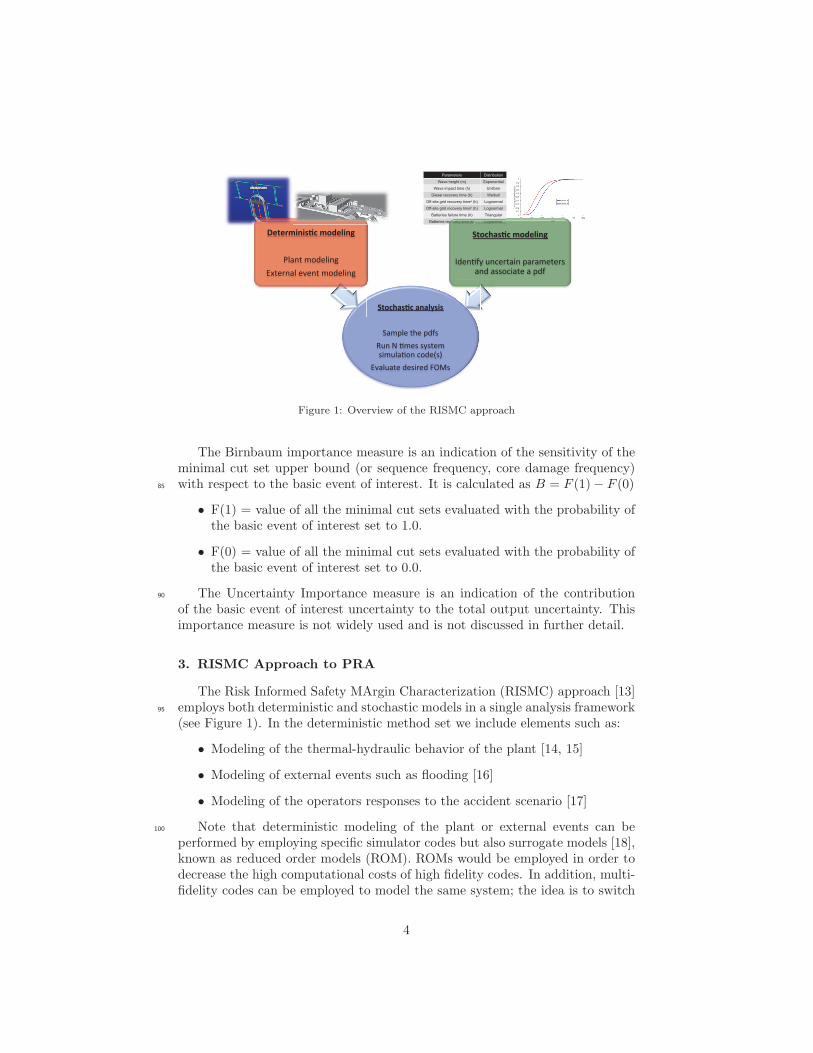
Figure 1: Overview of the RISMC approach
The Birnbaum importance measure is an indication of the sensitivity of theminimal cut set upper bound (or sequence frequency, core damage frequency)with respect to the basic event of interest. It is calculated as B = F (1)− F (0)85
• F(1) = value of all the minimal cut sets evaluated with the probability ofthe basic event of interest set to 1.0.
• F(0) = value of all the minimal cut sets evaluated with the probability ofthe basic event of interest set to 0.0.
The Uncertainty Importance measure is an indication of the contribution90
of the basic event of interest uncertainty to the total output uncertainty. Thisimportance measure is not widely used and is not discussed in further detail.
3. RISMC Approach to PRA
The Risk Informed Safety MArgin Characterization (RISMC) approach [13]employs both deterministic and stochastic models in a single analysis framework95
(see Figure 1). In the deterministic method set we include elements such as:
• Modeling of the thermal-hydraulic behavior of the plant [14, 15]
• Modeling of external events such as flooding [16]
• Modeling of the operators responses to the accident scenario [17]
Note that deterministic modeling of the plant or external events can be100
performed by employing specific simulator codes but also surrogate models [18],known as reduced order models (ROM). ROMs would be employed in order todecrease the high computational costs of high fidelity codes. In addition, multi-fidelity codes can be employed to model the same system; the idea is to switch
4
from low-fidelity to high-fidelity code when higher accuracy is needed (e.g., use105
low-fidelity codes for steady-state conditions and high-fidelity code for transientconditions)
In the stochastic modeling we include all stochastic parameters that areof interest in the PRA analysis such as uncertain parameters and stochasticfailure of system/components. As mentioned earlier, the RISMC approach relies110
on multi-physics system simulator codes (e.g., RELAP5-3D [10]) coupled withstochastic analysis tools (e.g., RAVEN [19]). From a PRA point of view, thistype of simulation can be described by using two sets of variables:
• c = c(t) represents the status of components and systems of the simulator(e.g., status of pumps and valves)115
• θ = θ(t) represents the temporal evolution of a simulated accident sce-nario, i.e., θ(t) represents a single simulation run. Each element of θ canbe for example the values of temperature or pressure in a specific node ofthe simulator nodalization.
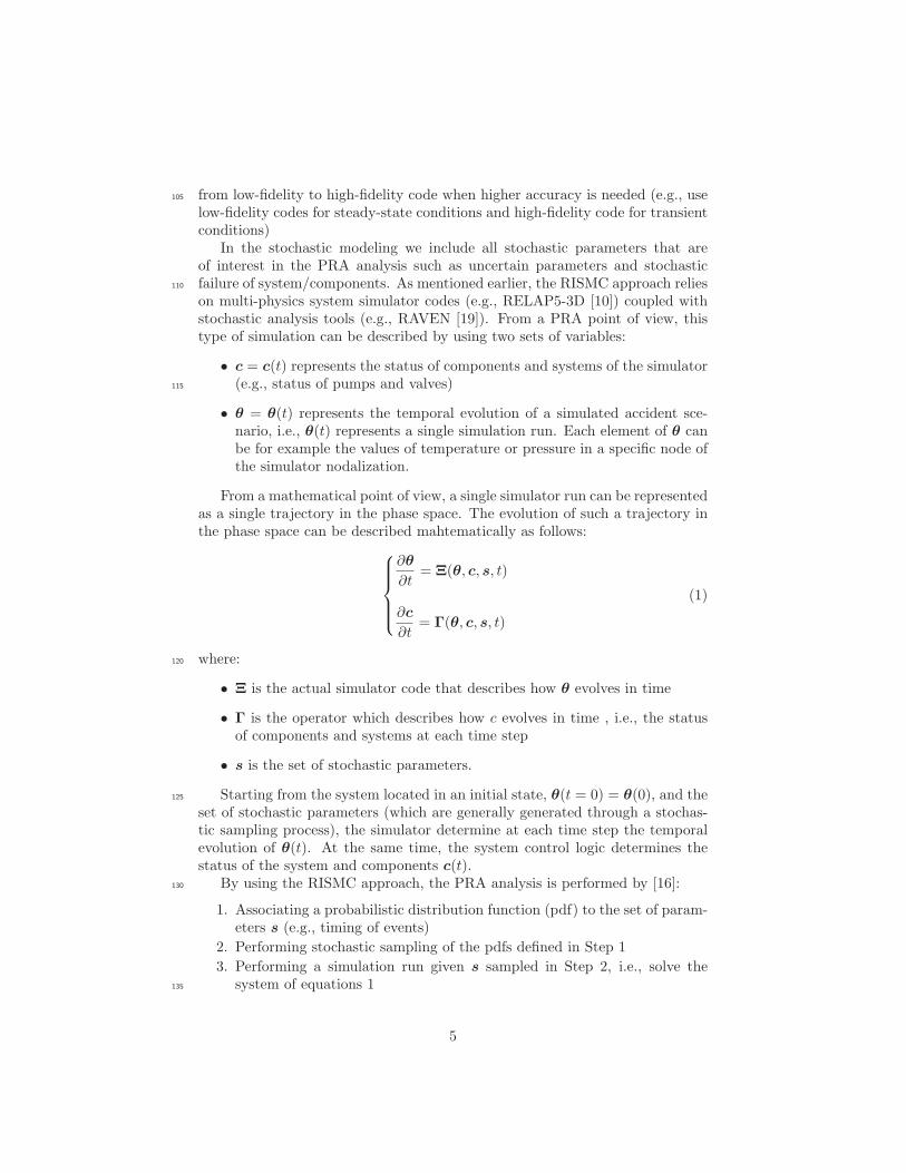
From a mathematical point of view, a single simulator run can be representedas a single trajectory in the phase space. The evolution of such a trajectory inthe phase space can be described mahtematically as follows:
⎧⎪⎪⎪⎨⎪⎪⎪⎩
∂θ
∂t= Ξ(θ, c, s, t)
∂c
∂t= Γ(θ, c, s, t)
(1)
where:120
• Ξ is the actual simulator code that describes how θ evolves in time
• Γ is the operator which describes how c evolves in time , i.e., the statusof components and systems at each time step
• s is the set of stochastic parameters.
Starting from the system located in an initial state, θ(t = 0) = θ(0), and the125
set of stochastic parameters (which are generally generated through a stochas-tic sampling process), the simulator determine at each time step the temporalevolution of θ(t). At the same time, the system control logic determines thestatus of the system and components c(t).
By using the RISMC approach, the PRA analysis is performed by [16]:130
1. Associating a probabilistic distribution function (pdf) to the set of param-eters s (e.g., timing of events)
2. Performing stochastic sampling of the pdfs defined in Step 1
3. Performing a simulation run given s sampled in Step 2, i.e., solve thesystem of equations 1135
5
4. Repeating Steps 2 and 3 M times and evaluating user defined stochasticparameters such as core damage (CD) probability (PCD).
Note that s includes not only uncertain parameters characteristic of thesimulator (e.g., pipe friction coefficients) but also the set Basic Events (BEs)associated to the considered components.140
The goal of measuring components risk importance is to identify the com-ponents that contribute the most to the system/plant overall risk.
The objective of this identification process once completed is that plant re-sources (e.g., procurement costs, maintenance, testing) can be directed towardsmore risk-significant components or they can be replaced with more reliable145
models while fewer resources can be allocated to components that are of lowerrisk.
3.1. RISMC Approach and Classical PRA
In a classical PRA framework, each BE has a unique probability value as-sociated to it (with possible uncertainty) while in a dynamic PRA each BE150
has a probability distribution function (pdf) associated to it. This pdf thatdescribes the stochastic behavior of the component can be discrete in nature(e.g.,a Bernoulli distribution) or continuous (e.g., exponential).
As an example lets consider two basic events associated to the emergencydiesel generators (EDGs) of a nuclear power plant: EDG failure to start (EDG FS)155
and EDG failure to run (EDG FS). In a classical PRA framework two proba-bility values would be associated to each basic event: pEDG FS and pEDG FR.In a dynamic PRA framework two pdfs would be associated to each basic event:
• EDG FS ∼ Bern(pEDG FS) (Bernoulli distribution representing success0 or failure 1)160
• EDG FR ∼ Exp(λEDG FR) (Exponential distribution representing thetime of failure).
When comparing Dynamic vs. Classical PRA approaches note the following:
• EDG FS has the identical statistical model in the two approaches
• EDG FR has different statistical models; however, if we set
pEDG FR =
∫ MT
0
λEDG FR · e−λEDG FRtdt (2)
where MT is the EDG mission time, then the two models are identical165
from a statistical perspective.
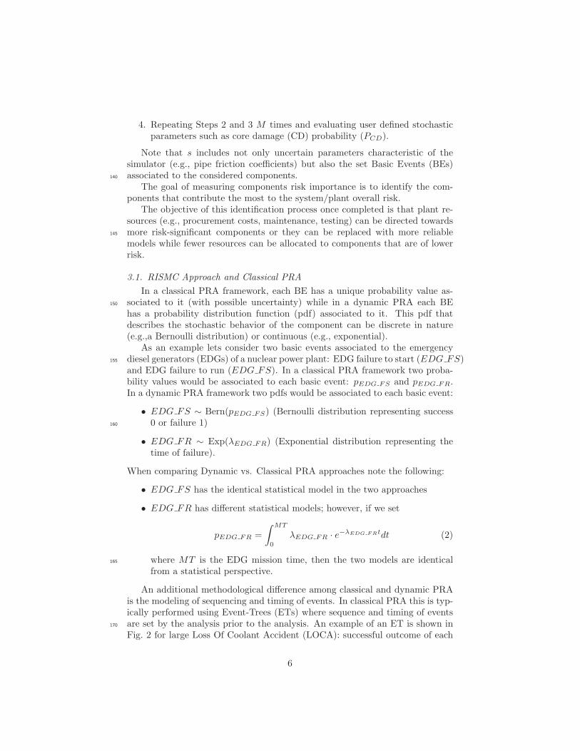
An additional methodological difference among classical and dynamic PRAis the modeling of sequencing and timing of events. In classical PRA this is typ-ically performed using Event-Trees (ETs) where sequence and timing of eventsare set by the analysis prior to the analysis. An example of an ET is shown in170
Fig. 2 for large Loss Of Coolant Accident (LOCA): successful outcome of each
6
IE-LLOCA
LARGE LOCA
ACC
ACCUMULATOR 2-OF-2
LPI
LOW PRESSURE INJECTION
FTF-LLOCALPR-LL
LOW PRESSURE RECIRCULATION
# End State(Phase - CD)
1 OK
2 CD
3 CD
4 CD
Figure 2: Large LOCA ET.
ET branch is guaranteed only if the accumulator, low-pressure injection (LPI)and low-pressure recirculation (LPR) systems successfully perform their func-tion. Each ET branch corresponds to a possible accident scenario while eachbranching point corresponds to the successful or failed activation of a system175
(accumulator, LPI and LPR) The ET construction requires the definition of aset of acceptance criteria (e.g., collapsed level greater than 1/3 of core height)and a set of success criteria for each system involved in the accident progression.This criteria are determined by the analysis and might be backed up by a setof thermal-hydraulic calculations.180
In a dynamic PRA method, timing and sequencing of events are uniquelydictated by the system control logic and by the set of stochastic parameterss,i.e., the construction of the ET is replaced by coding the plant control logic(e.g., system activation points and activation rules). In addition, acceptancecriteria and success criteria are incorporated into the physics model of the code185
Back to the large LOCA scenario, in a dynamic framework it would be modeledby:
• Employing a system simulator code (e.g., RELAP5-3D)
• Defining three stochastic parameters:
– accumulator system: failure on demand (Bernoulli distribution)190
– LPI system: failure to run (Exponential distribution)
– LPR system: failure to run (Exponential distribution)
• Setting the condition to end a code simulation run and its correspondingoutcome:
– OK outcome: mission time (e.g., 24 hours)195
– Fail outcome: maximum core temperature greater than 2200 F
Note that discrepancies among classical and dynamic PRA methods canoccur for sequence of events coupled with system dynamics. Assuming twoevents A and B occur in sequence and time of activation of each of them isa stochastic variable (tA ∼ pdfA(t) and tB ∼ pdfB(t)), the actual activation
7
time TB of system B is a stochastic variable given by the sum of tA and tB(TB = tA + tB). In a classical PRA framework, the distribution of TB (i.e.,pdfA+B(t)) can be determined by solving the convolution integral:
pdfA+B(t) =
∫ ∞
−∞pdfB(t− τ)pdfA(τ)dτ (3)
This convolution integral get more complex when accident progression includea large number of events and system dynamics affect timing of events.
4. RAVEN
The Risk Analysis and Virtual ENviroment (RAVEN1) [6, 19] is a flexible200
and multi-purpose uncertainty quantification, regression analysis, probabilisticrisk assessment, data analysis and model optimization framework. Dependingon the tasks to be accomplished and on the probabilistic characterization of theproblem, RAVEN perturbs (e.g., Monte-Carlo, latin hypercube, reliability sur-face search) the response of the system under consideration by altering its own205
parameters. The system is modeled by third party software (e.g., RELAP5-3D [10], MELCOR [11]) and accessible to RAVEN either directly (softwarecoupling) or indirectly (via input/output files). The data generated by thesampling process is analyzed using classical statistical and more advanced datamining approaches. RAVEN also manages the parallel dispatching (i.e. both on210
desktop/workstation and large High Performance Computing machines) of thesoftware representing the physical model. RAVEN heavily relies on artificial in-telligence algorithms to construct surrogate models of complex physical systemsin order to perform uncertainty quantification, reliability analysis (limit statesurface) and parametric studies.215
By statistical analysis we include:
• Sampling of codes, either stochastic, e.g., Monte-Carlo [20] and Latin Hy-percube Sampling (LHS) [21], deterministic (e.g., grid and Dynamic EventTree (DET) [22, 23]) or adaptive [24, 25]
• Generation of ROMs [18], also known as Surrogate models220
• Post-processing of the sampled data and generation of statistical param-eters (e.g., mean, variance, covariance matrix).
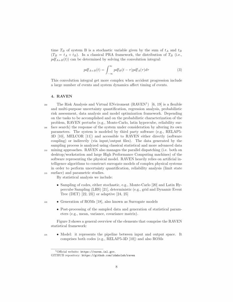
Figure 3 shows a general overview of the elements that comprise the RAVENstatistical framework:
• Model: it represents the pipeline between input and output space. It225
comprises both codes (e.g., RELAP5-3D [10]) and also ROMs
1Official website: https://raven.inl.gov,GITHUB repository: https://github.com/idaholab/raven
8
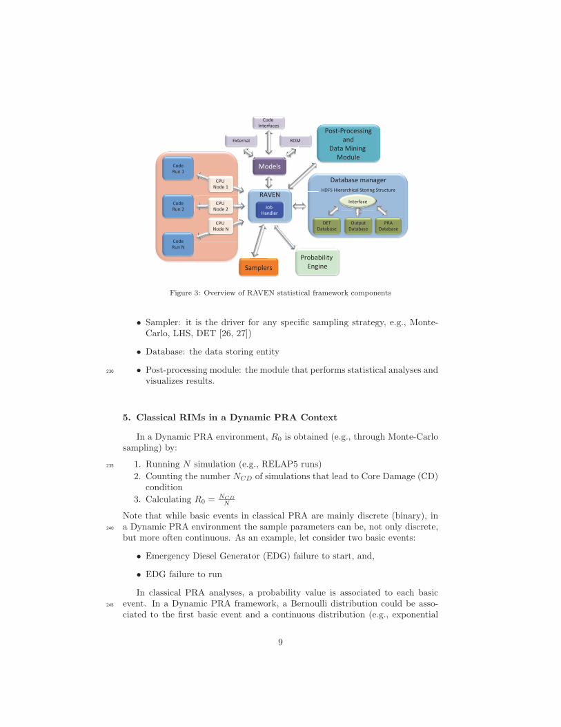
Figure 3: Overview of RAVEN statistical framework components
• Sampler: it is the driver for any specific sampling strategy, e.g., Monte-Carlo, LHS, DET [26, 27])
• Database: the data storing entity
• Post-processing module: the module that performs statistical analyses and230
visualizes results.
5. Classical RIMs in a Dynamic PRA Context
In a Dynamic PRA environment, R0 is obtained (e.g., through Monte-Carlosampling) by:
1. Running N simulation (e.g., RELAP5 runs)235
2. Counting the number NCD of simulations that lead to Core Damage (CD)condition
3. Calculating R0 = NCD
N
Note that while basic events in classical PRA are mainly discrete (binary), ina Dynamic PRA environment the sample parameters can be, not only discrete,240
but more often continuous. As an example, let consider two basic events:
• Emergency Diesel Generator (EDG) failure to start, and,
• EDG failure to run
In classical PRA analyses, a probability value is associated to each basicevent. In a Dynamic PRA framework, a Bernoulli distribution could be asso-245
ciated to the first basic event and a continuous distribution (e.g., exponential
9
distribution) could be associated to the second basic event. At this point achallenge arises: the determination of R−
i and R+i for each sampled parameter;
two possible approaches can be followed :
1. Perform a Dynamic PRA for R0 and each R−i and R+
i (requiring three250
times the number of calculations)
2. Determine an approximated value of R−i and R+
i from the simulation runsgenerated to calculate R0
Regarding Approach 1, given the computational costs of each Dynamic PRA,it is inefficient to determine R−
i and R+i for each sampled parameter. In fact, if255
we consider S sample parameters (i.e., S basic events) over N simulations, thenthe risk importance analysis would require N(2S + 1) simulations.
Regarding Approach 2, a unique method (implemented in RAVEN as aninternal post-processor) was developed and it is presented. This method requiresinput from the user:260
• Range, I−i , of the variable si that can be associated to the statement“basic event with component perfectly reliable”
• Range, I+i , of the variable si that can be associated to the statement“basic event in a failed status”
Note that the reason we require these types of input in the dynamic analyses is265
that the parameter space is defined as a continuum unlike the discrete Booleanspace found in classical PRA.
Given this kind of information, it is possible to calculate R+i and R−
i asfollows:
R0 =NCD
N(4)
R+i =
NCD,si∈I+i
N(5)
R−i =
NCD,si∈I−i
N(6)
where:
• NCD,si∈I+iis the number of simulations leading to core damage and with
parameter si ∈ I+i270
• NCD,si∈I−i
is the number of simulations leading to core damage and with
parameter si ∈ I−i
Since these measures are condtioned on the choices of I+i and I−i , dependingon their values, R+
i and R−i might change accordingly. In addition, the statisti-
cal error associated to the estimates of R+i and R−
i also changes as a function of275
the sampling process. An example is shown in Figure 4 for both cases (discreteand continuous) of a basic event xi represented as a stochastic variable which
10
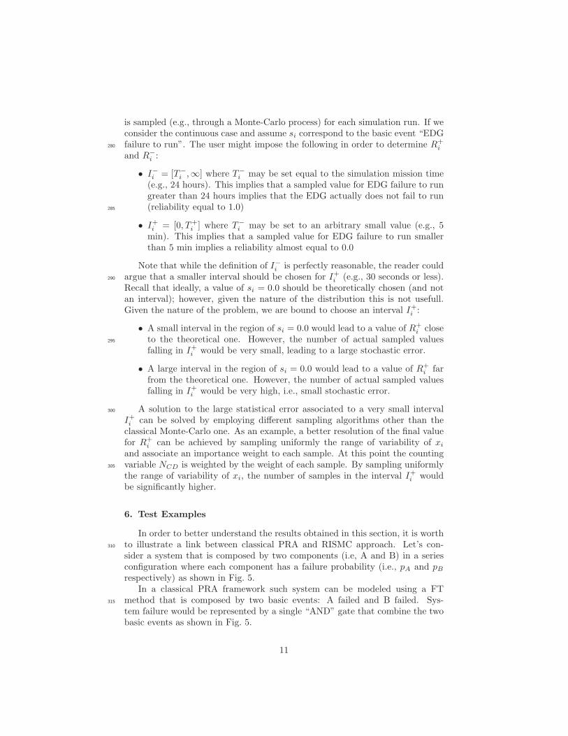
is sampled (e.g., through a Monte-Carlo process) for each simulation run. If weconsider the continuous case and assume si correspond to the basic event “EDGfailure to run”. The user might impose the following in order to determine R+
i280
and R−i :
• I−i = [T−i ,∞] where T−
i may be set equal to the simulation mission time(e.g., 24 hours). This implies that a sampled value for EDG failure to rungreater than 24 hours implies that the EDG actually does not fail to run(reliability equal to 1.0)285
• I+i = [0, T+i ] where T−
i may be set to an arbitrary small value (e.g., 5min). This implies that a sampled value for EDG failure to run smallerthan 5 min implies a reliability almost equal to 0.0
Note that while the definition of I−i is perfectly reasonable, the reader couldargue that a smaller interval should be chosen for I+i (e.g., 30 seconds or less).290
Recall that ideally, a value of si = 0.0 should be theoretically chosen (and notan interval); however, given the nature of the distribution this is not usefull.Given the nature of the problem, we are bound to choose an interval I+i :
• A small interval in the region of si = 0.0 would lead to a value of R+i close
to the theoretical one. However, the number of actual sampled values295
falling in I+i would be very small, leading to a large stochastic error.
• A large interval in the region of si = 0.0 would lead to a value of R+i far
from the theoretical one. However, the number of actual sampled valuesfalling in I+i would be very high, i.e., small stochastic error.
A solution to the large statistical error associated to a very small interval300
I+i can be solved by employing different sampling algorithms other than theclassical Monte-Carlo one. As an example, a better resolution of the final valuefor R+
i can be achieved by sampling uniformly the range of variability of xi
and associate an importance weight to each sample. At this point the countingvariable NCD is weighted by the weight of each sample. By sampling uniformly305
the range of variability of xi, the number of samples in the interval I+i wouldbe significantly higher.
6. Test Examples
In order to better understand the results obtained in this section, it is worthto illustrate a link between classical PRA and RISMC approach. Let’s con-310
sider a system that is composed by two components (i.e, A and B) in a seriesconfiguration where each component has a failure probability (i.e., pA and pBrespectively) as shown in Fig. 5.
In a classical PRA framework such system can be modeled using a FTmethod that is composed by two basic events: A failed and B failed. Sys-315
tem failure would be represented by a single “AND” gate that combine the twobasic events as shown in Fig. 5.
11
pdfi
xi 0 xi+ xi
-
Ii+ Ii-
pdfi
xi 0 xi+ xi
-
Ii+ Ii-
Reliability = 1.0 Reliability = 0.0
Reliability = 1.0 Reliability = 0.0
Figure 4: Treatment of discrete (top) and continuous (bottom) stochastic variables for relia-bility purposes.
12
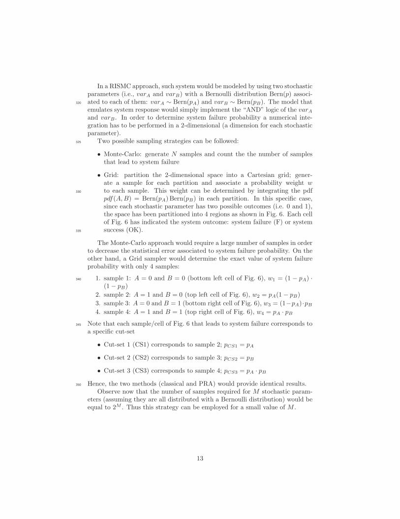
In a RISMC approach, such system would be modeled by using two stochasticparameters (i.e., varA and varB) with a Bernoulli distribution Bern(p) associ-ated to each of them: varA ∼ Bern(pA) and varB ∼ Bern(pB). The model that320
emulates system response would simply implement the “AND” logic of the varAand varB . In order to determine system failure probability a numerical inte-gration has to be performed in a 2-dimensional (a dimension for each stochasticparameter).
Two possible sampling strategies can be followed:325
• Monte-Carlo: generate N samples and count the the number of samplesthat lead to system failure
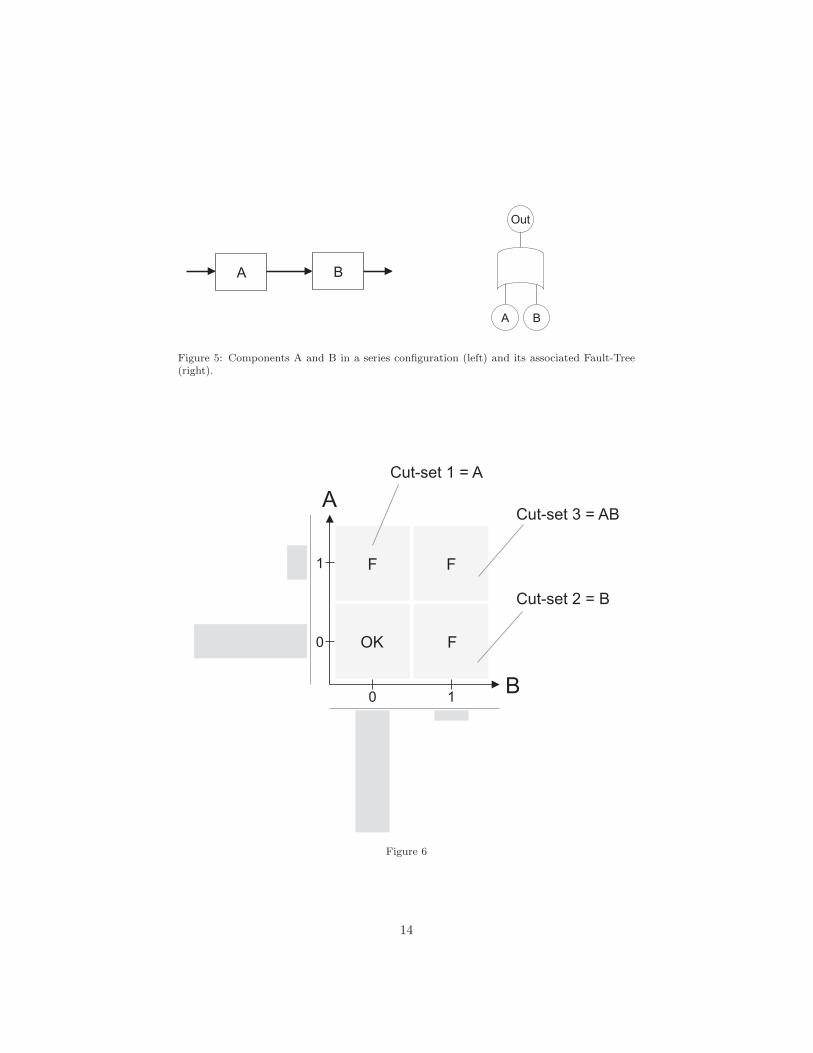
• Grid: partition the 2-dimensional space into a Cartesian grid; gener-ate a sample for each partition and associate a probability weight wto each sample. This weight can be determined by integrating the pdf330
pdf(A,B) = Bern(pA) Bern(pB) in each partition. In this specific case,since each stochastic parameter has two possible outcomes (i.e. 0 and 1),the space has been partitioned into 4 regions as shown in Fig. 6. Each cellof Fig. 6 has indicated the system outcome: system failure (F) or systemsuccess (OK).335
The Monte-Carlo approach would require a large number of samples in orderto decrease the statistical error associated to system failure probability. On theother hand, a Grid sampler would determine the exact value of system failureprobability with only 4 samples:
1. sample 1: A = 0 and B = 0 (bottom left cell of Fig. 6), w1 = (1 − pA) ·340
(1− pB)
2. sample 2: A = 1 and B = 0 (top left cell of Fig. 6), w2 = pA(1− pB)
3. sample 3: A = 0 and B = 1 (bottom right cell of Fig. 6), w3 = (1−pA) ·pB4. sample 4: A = 1 and B = 1 (top right cell of Fig. 6), w4 = pA · pB
Note that each sample/cell of Fig. 6 that leads to system failure corresponds to345
a specific cut-set
• Cut-set 1 (CS1) corresponds to sample 2; pCS1 = pA
• Cut-set 2 (CS2) corresponds to sample 3; pCS2 = pB
• Cut-set 3 (CS3) corresponds to sample 4; pCS3 = pA · pBHence, the two methods (classical and PRA) would provide identical results.350
Observe now that the number of samples required for M stochastic param-eters (assuming they are all distributed with a Bernoulli distribution) would beequal to 2M . Thus this strategy can be employed for a small value of M .
13
A B
Figure 5: Components A and B in a series configuration (left) and its associated Fault-Tree(right).
A
B
0
1
0 1
OK F
F F
Cut-set 1 = A
Cut-set 2 = B
Cut-set 3 = AB
Figure 6
14
A
B
C
Figure 7: System considered for Examples 1 and 2.
SYS1
SYSTEM FOR TEST CASE 1
CASE11
FAILURE OF BOTH B AND C
5.0000E-02B-FTS
COMPONENT B FAILS TO START
1.0000E-01C-FTS
COMPONENT C FAILS TO START
1.0000E-02A-FTS
COMPONENT A FAILS TO START
Figure 8: FT structure for the system shown in Fig. 7.
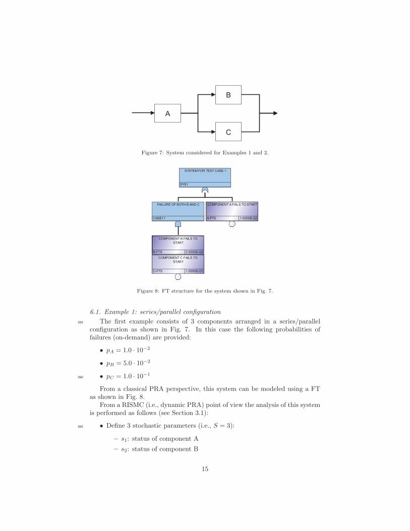
6.1. Example 1: series/parallel configuration
The first example consists of 3 components arranged in a series/parallel355
configuration as shown in Fig. 7. In this case the following probabilities offailures (on-demand) are provided:
• pA = 1.0 · 10−2
• pB = 5.0 · 10−2
• pC = 1.0 · 10−1360
From a classical PRA perspective, this system can be modeled using a FTas shown in Fig. 8.
From a RISMC (i.e., dynamic PRA) point of view the analysis of this systemis performed as follows (see Section 3.1):
• Define 3 stochastic parameters (i.e., S = 3):365
– s1: status of component A
– s2: status of component B
15
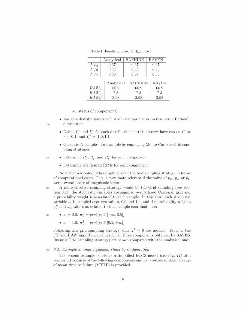
Table 1: Results obtained for Example 1.
Analytical SAPHIRE RAVENFVA 0.67 0.67 0.67FVB 0.33 0.34 0.33FVC 0.33 0.34 0.33
Analytical SAPHIRE RAVENRAWA 66.9 66.9 66.9RAWB 7.3 7.3 7.3RAWC 3.98 3.98 3.98
– s3: status of component C
• Assign a distribution to each stochastic parameter; in this case a Bernoullidistribution370
• Define I+i and I−i for each distribution: in this case we have chosen I−i =[0.0, 0.1] and I+i = [1.0, 1.1]
• Generate N samples, for example by employing Monte-Carlo or Grid sam-pling strategies
• Determine R0, R−i and R+
i for each component375
• Determine the desired RIMs for each component
Note that a Monte-Carlo sampling is not the best sampling strategy in termsof computational costs. This is even more relevant if the value of pA, pB or pCwere several order of magnitude lower.
A more effective sampling strategy would be the Grid sampling (see Sec-380
tion 3.1): the stochastic variables are sampled over a fixed Cartesian grid anda probability weight is associated to each sample. In this case, each stochasticvariable si is sampled over two values, 0.0 and 1.0, and the probability weightsw0
i and w1i values associated to each sample coordinate are:
• si = 0.0: w0i = prob(si ∈ [−∞, 0.5])385
• si = 1.0: w1i = prob(si ∈ [0.5,+∞])
Following this grid sampling strategy, only 23 = 8 are needed. Table 1, theFV and RAW importance values for all three components obtained by RAVEN(using a Grid sampling strategy) are shown compared with the analytical ones.
6.2. Example 2: time-dependent stand-by configuration390
The second example considers a simplified ECCS model (see Fig. ??) of areactor. It consists of the following components and for a subset of them a valueof mean time to failure (MTTF) is provided:
16
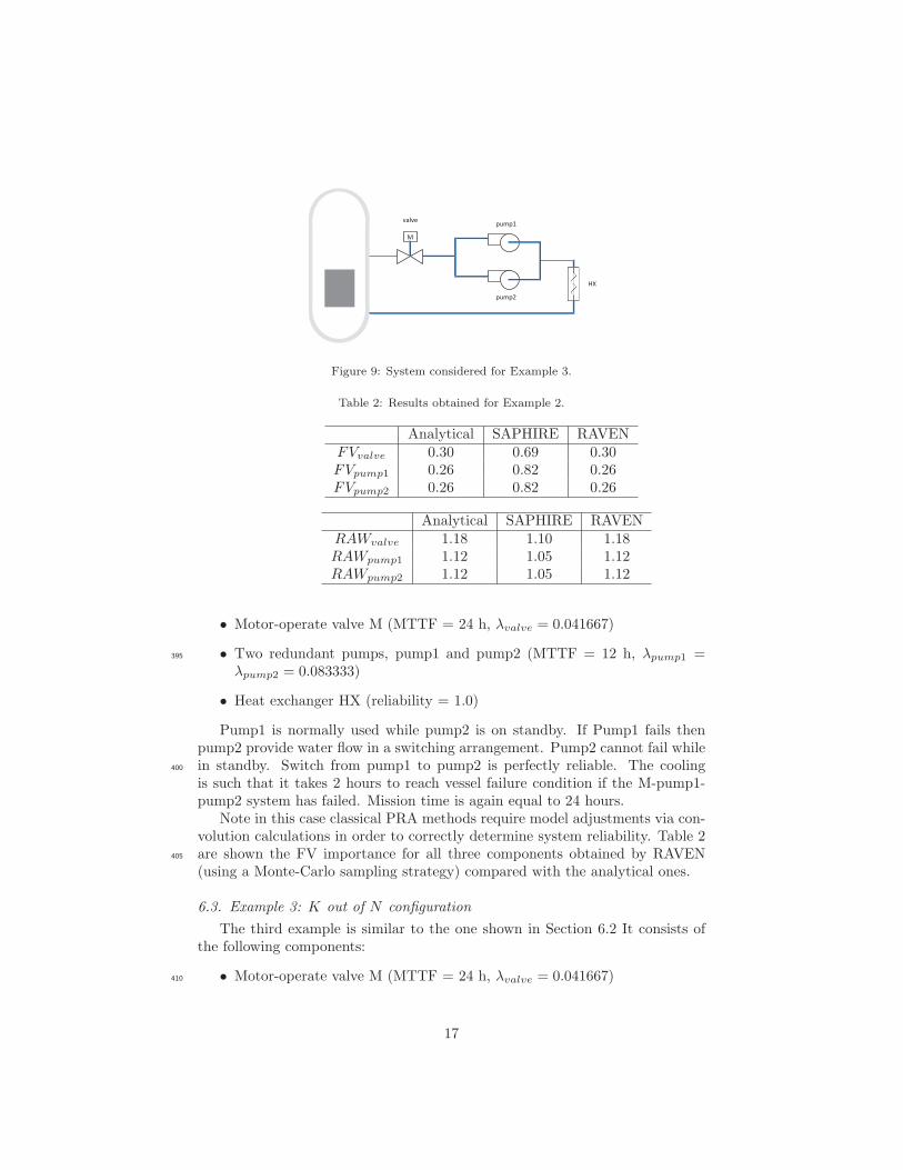
Figure 9: System considered for Example 3.
Table 2: Results obtained for Example 2.
Analytical SAPHIRE RAVENFVvalve 0.30 0.69 0.30FVpump1 0.26 0.82 0.26FVpump2 0.26 0.82 0.26
Analytical SAPHIRE RAVENRAWvalve 1.18 1.10 1.18RAWpump1 1.12 1.05 1.12RAWpump2 1.12 1.05 1.12
• Motor-operate valve M (MTTF = 24 h, λvalve = 0.041667)
• Two redundant pumps, pump1 and pump2 (MTTF = 12 h, λpump1 =395
λpump2 = 0.083333)
• Heat exchanger HX (reliability = 1.0)
Pump1 is normally used while pump2 is on standby. If Pump1 fails thenpump2 provide water flow in a switching arrangement. Pump2 cannot fail whilein standby. Switch from pump1 to pump2 is perfectly reliable. The cooling400
is such that it takes 2 hours to reach vessel failure condition if the M-pump1-pump2 system has failed. Mission time is again equal to 24 hours.
Note in this case classical PRA methods require model adjustments via con-volution calculations in order to correctly determine system reliability. Table 2are shown the FV importance for all three components obtained by RAVEN405
(using a Monte-Carlo sampling strategy) compared with the analytical ones.
6.3. Example 3: K out of N configuration
The third example is similar to the one shown in Section 6.2 It consists ofthe following components:
• Motor-operate valve M (MTTF = 24 h, λvalve = 0.041667)410
17
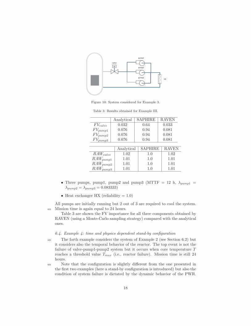
Figure 10: System considered for Example 3.
Table 3: Results obtained for Example III.
Analytical SAPHIRE RAVENFVvalve 0.032 0.64 0.033FVpump1 0.076 0.94 0.081FVpump2 0.076 0.94 0.081FVpump3 0.076 0.94 0.081
Analytical SAPHIRE RAVENRAWvalve 1.02 1.0 1.02RAWpump1 1.01 1.0 1.01RAWpump2 1.01 1.0 1.01RAWpump3 1.01 1.0 1.01
• Three pumps, pump1, pump2 and pump3 (MTTF = 12 h, λpump1 =λpump2 = λpump3 = 0.083333)
• Heat exchanger HX (reliability = 1.0)
All pumps are initially running but 2 out of 3 are required to cool the system.Mission time is again equal to 24 hours.415
Table 3 are shown the FV importance for all three components obtained byRAVEN (using a Monte-Carlo sampling strategy) compared with the analyticalones.
6.4. Example 4: time and physics dependent stand-by configuration
The forth example considers the system of Example 2 (see Section 6.2) but420
it considers also the temporal behavior of the reactor. The top event is not thefailure of valve-pump1-pump2 system but it occurs when core temperature Treaches a threshold value Tmax (i.e., reactor failure). Mission time is still 24hours.
Note that the configuration is slightly different from the one presented in425
the first two examples (here a stand-by configuration is introduced) but also thecondition of system failure is dictated by the dynamic behavior of the PWR.
18
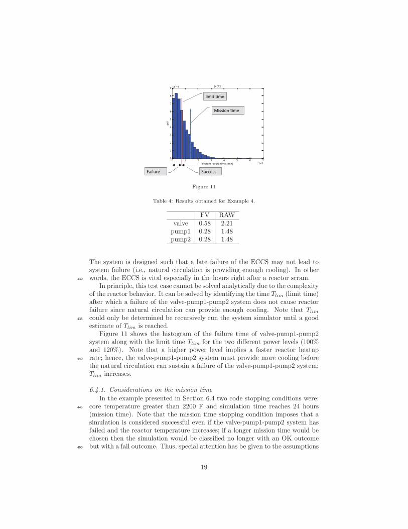
Figure 11
Table 4: Results obtained for Example 4.
FV RAWvalve 0.58 2.21pump1 0.28 1.48pump2 0.28 1.48
The system is designed such that a late failure of the ECCS may not lead tosystem failure (i.e., natural circulation is providing enough cooling). In otherwords, the ECCS is vital especially in the hours right after a reactor scram.430
In principle, this test case cannot be solved analytically due to the complexityof the reactor behavior. It can be solved by identifying the time Tlim (limit time)after which a failure of the valve-pump1-pump2 system does not cause reactorfailure since natural circulation can provide enough cooling. Note that Tlim
could only be determined be recursively run the system simulator until a good435
estimate of Tlim is reached.Figure 11 shows the histogram of the failure time of valve-pump1-pump2
system along with the limit time Tlim for the two different power levels (100%and 120%). Note that a higher power level implies a faster reactor heatuprate; hence, the valve-pump1-pump2 system must provide more cooling before440
the natural circulation can sustain a failure of the valve-pump1-pump2 system:Tlim increases.
6.4.1. Considerations on the mission time
In the example presented in Section 6.4 two code stopping conditions were:core temperature greater than 2200 F and simulation time reaches 24 hours445
(mission time). Note that the mission time stopping condition imposes that asimulation is considered successful even if the valve-pump1-pump2 system hasfailed and the reactor temperature increases; if a longer mission time would bechosen then the simulation would be classified no longer with an OK outcomebut with a fail outcome. Thus, special attention has be given to the assumptions450
19
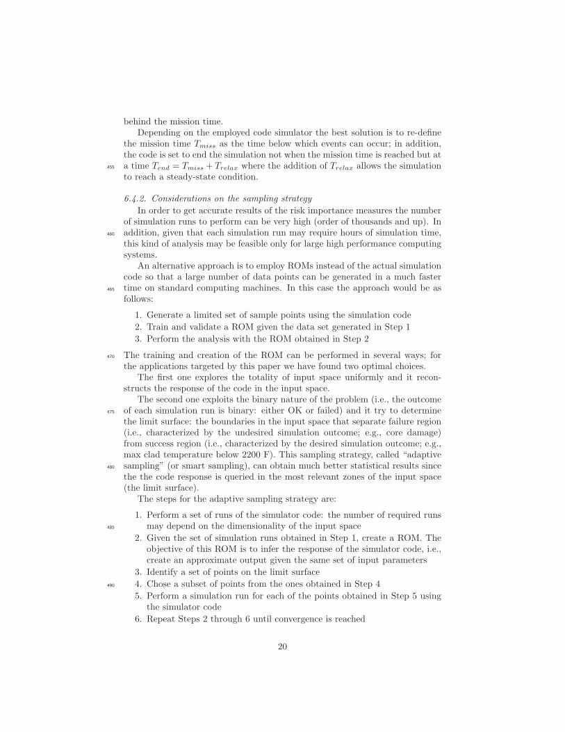
behind the mission time.Depending on the employed code simulator the best solution is to re-define
the mission time Tmiss as the time below which events can occur; in addition,the code is set to end the simulation not when the mission time is reached but ata time Tend = Tmiss + Trelax where the addition of Trelax allows the simulation455
to reach a steady-state condition.
6.4.2. Considerations on the sampling strategy
In order to get accurate results of the risk importance measures the numberof simulation runs to perform can be very high (order of thousands and up). Inaddition, given that each simulation run may require hours of simulation time,460
this kind of analysis may be feasible only for large high performance computingsystems.
An alternative approach is to employ ROMs instead of the actual simulationcode so that a large number of data points can be generated in a much fastertime on standard computing machines. In this case the approach would be as465
follows:
1. Generate a limited set of sample points using the simulation code
2. Train and validate a ROM given the data set generated in Step 1
3. Perform the analysis with the ROM obtained in Step 2
The training and creation of the ROM can be performed in several ways; for470
the applications targeted by this paper we have found two optimal choices.The first one explores the totality of input space uniformly and it recon-
structs the response of the code in the input space.The second one exploits the binary nature of the problem (i.e., the outcome
of each simulation run is binary: either OK or failed) and it try to determine475
the limit surface: the boundaries in the input space that separate failure region(i.e., characterized by the undesired simulation outcome; e.g., core damage)from success region (i.e., characterized by the desired simulation outcome; e.g.,max clad temperature below 2200 F). This sampling strategy, called “adaptivesampling” (or smart sampling), can obtain much better statistical results since480
the the code response is queried in the most relevant zones of the input space(the limit surface).
The steps for the adaptive sampling strategy are:
1. Perform a set of runs of the simulator code: the number of required runsmay depend on the dimensionality of the input space485
2. Given the set of simulation runs obtained in Step 1, create a ROM. Theobjective of this ROM is to infer the response of the simulator code, i.e.,create an approximate output given the same set of input parameters
3. Identify a set of points on the limit surface
4. Chose a subset of points from the ones obtained in Step 4490
5. Perform a simulation run for each of the points obtained in Step 5 usingthe simulator code
6. Repeat Steps 2 through 6 until convergence is reached
20
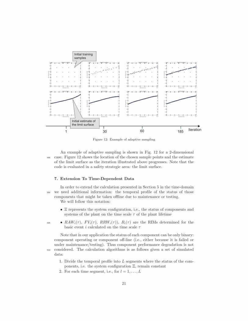
Iteration 1 30 60 185
Initial training samples
Initial estimate of the limit surface
Figure 12: Example of adaptive sampling
An example of adaptive sampling is shown in Fig. 12 for a 2-dimensionalcase. Figure 12 shows the location of the chosen sample points and the estimate495
of the limit surface as the iteration illustrated above progresses. Note that thecode is evaluated in a safety strategic area: the limit surface.
7. Extension To Time-Dependent Data
In order to extend the calculation presented in Section 5 in the time-domainwe need additional information: the temporal profile of the status of those500
components that might be taken offline due to maintenance or testing.We will follow this notation:
• Ξ represents the system configuration, i.e., the status of components andsystems of the plant on the time scale τ of the plant lifetime
• RAWi(τ), FVi(τ), RRWi(τ)), Bi(τ) are the RIMs determined for the505
basic event i calculated on the time scale τ
Note that in our application the status of each component can be only binary:component operating or component off-line (i.e., either because it is failed orunder maintenance/testing). Thus component performance degradation is notconsidered. The calculation algorithms is as follows given a set of simulated510
data:
1. Divide the temporal profile into L segments where the status of the com-ponents, i.e. the system configuration Ξ, remain constant
2. For each time segment, i.e., for l = 1, . . . , L
21
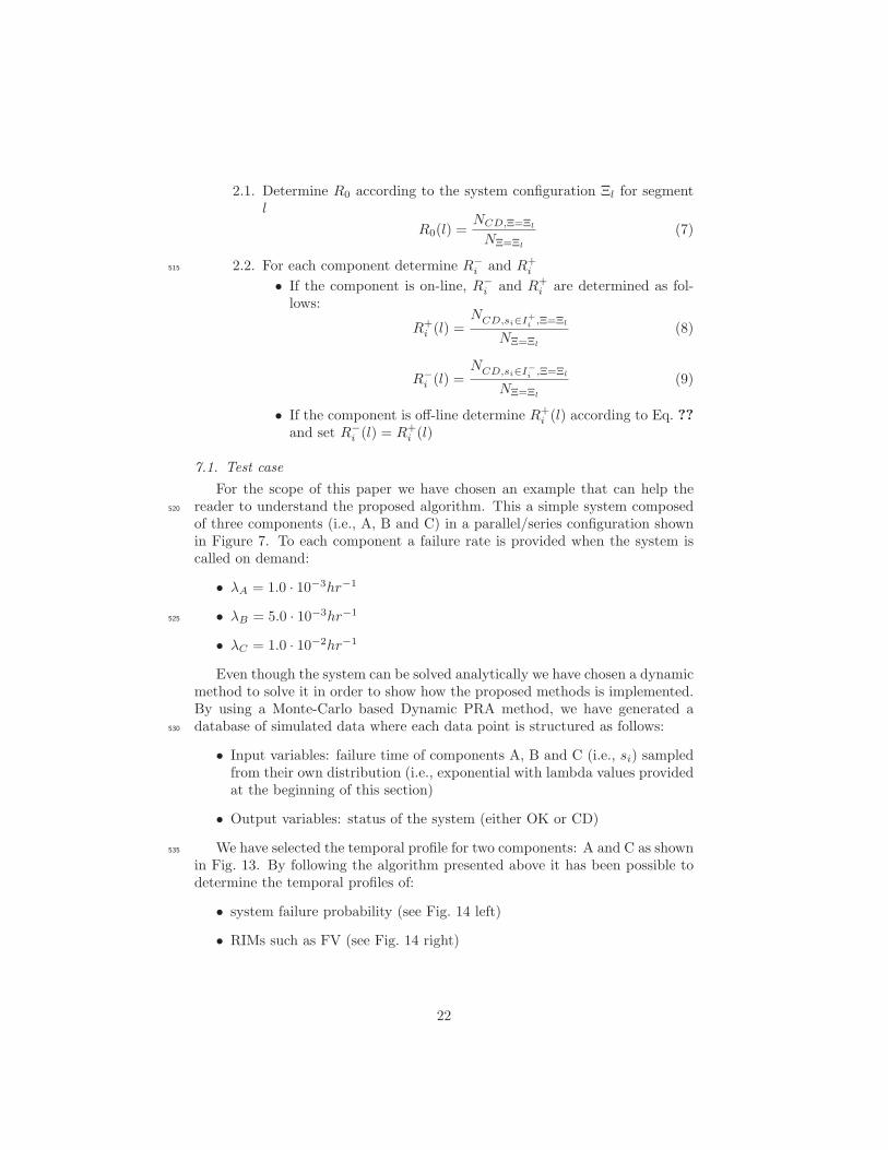
2.1. Determine R0 according to the system configuration Ξl for segmentl
R0(l) =NCD,Ξ=Ξl
NΞ=Ξl
(7)
2.2. For each component determine R−i and R+
i515
• If the component is on-line, R−i and R+
i are determined as fol-lows:
R+i (l) =
NCD,si∈I+i ,Ξ=Ξl
NΞ=Ξl
(8)
R−i (l) =
NCD,si∈I−i ,Ξ=Ξl
NΞ=Ξl
(9)
• If the component is off-line determine R+i (l) according to Eq. ??
and set R−i (l) = R+
i (l)
7.1. Test case
For the scope of this paper we have chosen an example that can help thereader to understand the proposed algorithm. This a simple system composed520
of three components (i.e., A, B and C) in a parallel/series configuration shownin Figure 7. To each component a failure rate is provided when the system iscalled on demand:
• λA = 1.0 · 10−3hr−1
• λB = 5.0 · 10−3hr−1525
• λC = 1.0 · 10−2hr−1
Even though the system can be solved analytically we have chosen a dynamicmethod to solve it in order to show how the proposed methods is implemented.By using a Monte-Carlo based Dynamic PRA method, we have generated adatabase of simulated data where each data point is structured as follows:530
• Input variables: failure time of components A, B and C (i.e., si) sampledfrom their own distribution (i.e., exponential with lambda values providedat the beginning of this section)
• Output variables: status of the system (either OK or CD)
We have selected the temporal profile for two components: A and C as shown535
in Fig. 13. By following the algorithm presented above it has been possible todetermine the temporal profiles of:
• system failure probability (see Fig. 14 left)
• RIMs such as FV (see Fig. 14 right)
22
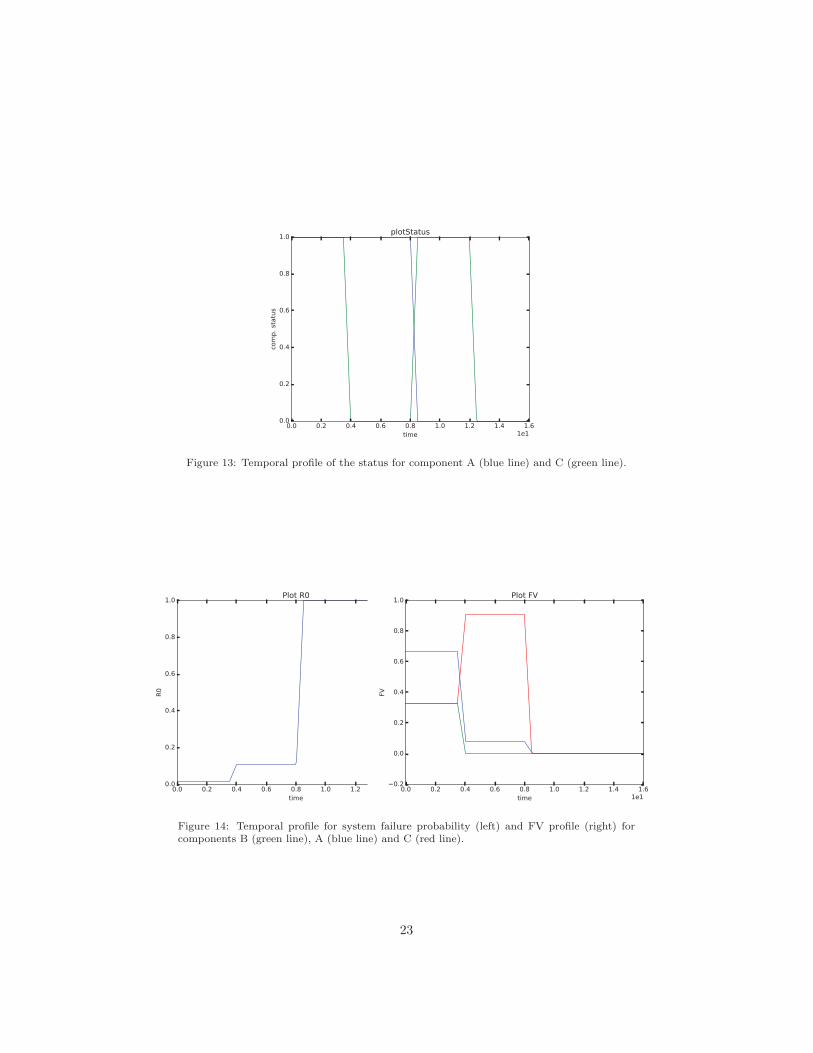
Figure 13: Temporal profile of the status for component A (blue line) and C (green line).
Figure 14: Temporal profile for system failure probability (left) and FV profile (right) forcomponents B (green line), A (blue line) and C (red line).
23
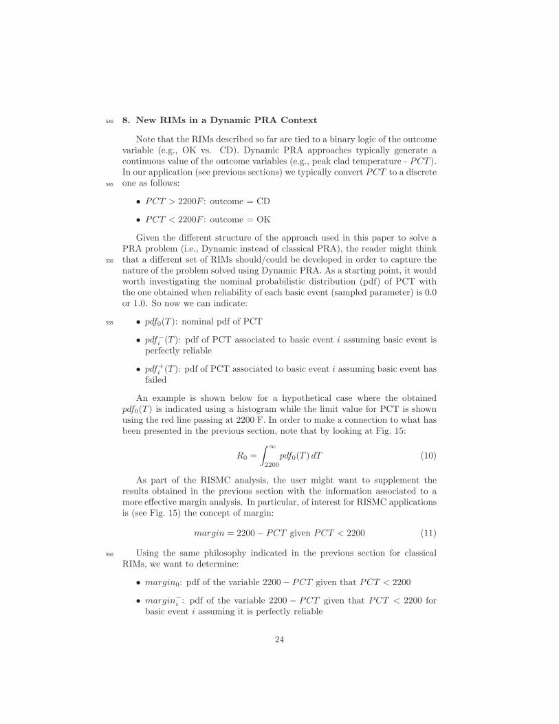
8. New RIMs in a Dynamic PRA Context540
Note that the RIMs described so far are tied to a binary logic of the outcomevariable (e.g., OK vs. CD). Dynamic PRA approaches typically generate acontinuous value of the outcome variables (e.g., peak clad temperature - PCT ).In our application (see previous sections) we typically convert PCT to a discreteone as follows:545
• PCT > 2200F : outcome = CD
• PCT < 2200F : outcome = OK
Given the different structure of the approach used in this paper to solve aPRA problem (i.e., Dynamic instead of classical PRA), the reader might thinkthat a different set of RIMs should/could be developed in order to capture the550
nature of the problem solved using Dynamic PRA. As a starting point, it wouldworth investigating the nominal probabilistic distribution (pdf) of PCT withthe one obtained when reliability of each basic event (sampled parameter) is 0.0or 1.0. So now we can indicate:
• pdf0(T ): nominal pdf of PCT555
• pdf−i (T ): pdf of PCT associated to basic event i assuming basic event is
perfectly reliable
• pdf+i (T ): pdf of PCT associated to basic event i assuming basic event has
failed
An example is shown below for a hypothetical case where the obtainedpdf0(T ) is indicated using a histogram while the limit value for PCT is shownusing the red line passing at 2200 F. In order to make a connection to what hasbeen presented in the previous section, note that by looking at Fig. 15:
R0 =
∫ ∞
2200
pdf0(T ) dT (10)
As part of the RISMC analysis, the user might want to supplement theresults obtained in the previous section with the information associated to amore effective margin analysis. In particular, of interest for RISMC applicationsis (see Fig. 15) the concept of margin:
margin = 2200− PCT given PCT < 2200 (11)
Using the same philosophy indicated in the previous section for classical560
RIMs, we want to determine:
• margin0: pdf of the variable 2200− PCT given that PCT < 2200
• margin−i : pdf of the variable 2200 − PCT given that PCT < 2200 for
basic event i assuming it is perfectly reliable
24
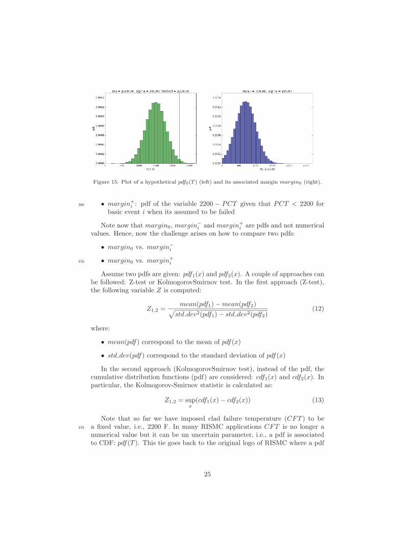
Figure 15: Plot of a hypothetical pdf0(T ) (left) and its associated margin margin0 (right).
• margin+i : pdf of the variable 2200 − PCT given that PCT < 2200 for565
basic event i when its assumed to be failed
Note now that margin0, margin−i and margin+
i are pdfs and not numericalvalues. Hence, now the challenge arises on how to compare two pdfs:
• margin0 vs. margin−i
• margin0 vs. margin+i570
Assume two pdfs are given: pdf1(x) and pdf2(x). A couple of approaches canbe followed: Z-test or KolmogorovSmirnov test. In the first approach (Z-test),the following variable Z is computed:
Z1,2 =mean(pdf1)−mean(pdf2)√
std dev2(pdf1)− std dev2(pdf2)(12)
where:
• mean(pdf) correspond to the mean of pdf(x)
• std dev(pdf) correspond to the standard deviation of pdf(x)
In the second approach (KolmogorovSmirnov test), instead of the pdf, thecumulative distribution functions (pdf) are considered: cdf1(x) and cdf2(x). Inparticular, the Kolmogorov-Smirnov statistic is calculated as:
Z1,2 = supx(cdf1(x)− cdf2(x)) (13)
Note that so far we have imposed clad failure temperature (CFT ) to bea fixed value, i.e., 2200 F. In many RISMC applications CFT is no longer a575
numerical value but it can be un uncertain parameter, i.e., a pdf is associatedto CDF: pdf(T ). This tie goes back to the original logo of RISMC where a pdf
25
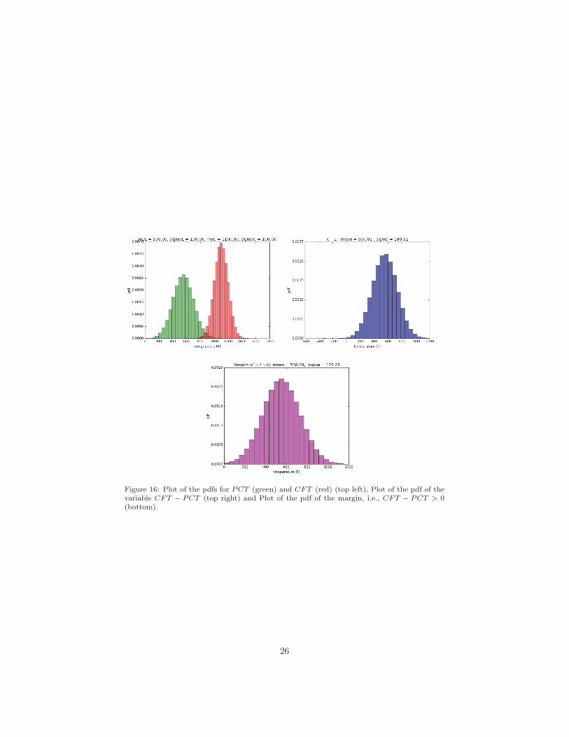
Figure 16: Plot of the pdfs for PCT (green) and CFT (red) (top left), Plot of the pdf of thevariable CFT − PCT (top right) and Plot of the pdf of the margin, i.e., CFT − PCT > 0(bottom).
26
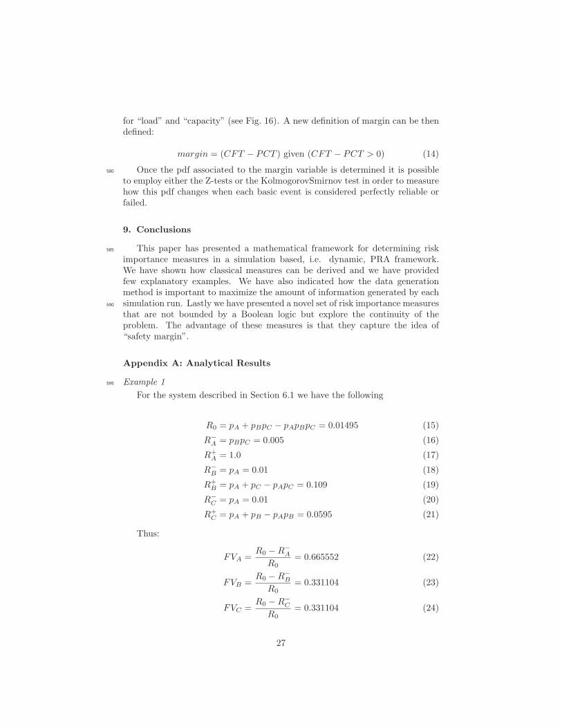
for “load” and “capacity” (see Fig. 16). A new definition of margin can be thendefined:
margin = (CFT − PCT ) given (CFT − PCT > 0) (14)
Once the pdf associated to the margin variable is determined it is possible580
to employ either the Z-tests or the KolmogorovSmirnov test in order to measurehow this pdf changes when each basic event is considered perfectly reliable orfailed.
9. Conclusions
This paper has presented a mathematical framework for determining risk585
importance measures in a simulation based, i.e. dynamic, PRA framework.We have shown how classical measures can be derived and we have providedfew explanatory examples. We have also indicated how the data generationmethod is important to maximize the amount of information generated by eachsimulation run. Lastly we have presented a novel set of risk importance measures590
that are not bounded by a Boolean logic but explore the continuity of theproblem. The advantage of these measures is that they capture the idea of“safety margin”.
Appendix A: Analytical Results
Example 1595
For the system described in Section 6.1 we have the following
R0 = pA + pBpC − pApBpC = 0.01495 (15)
R−A = pBpC = 0.005 (16)
R+A = 1.0 (17)
R−B = pA = 0.01 (18)
R+B = pA + pC − pApC = 0.109 (19)
R−C = pA = 0.01 (20)
R+C = pA + pB − pApB = 0.0595 (21)
Thus:
FVA =R0 −R−
A
R0= 0.665552 (22)
FVB =R0 −R−
B
R0= 0.331104 (23)
FVC =R0 −R−
C
R0= 0.331104 (24)
27
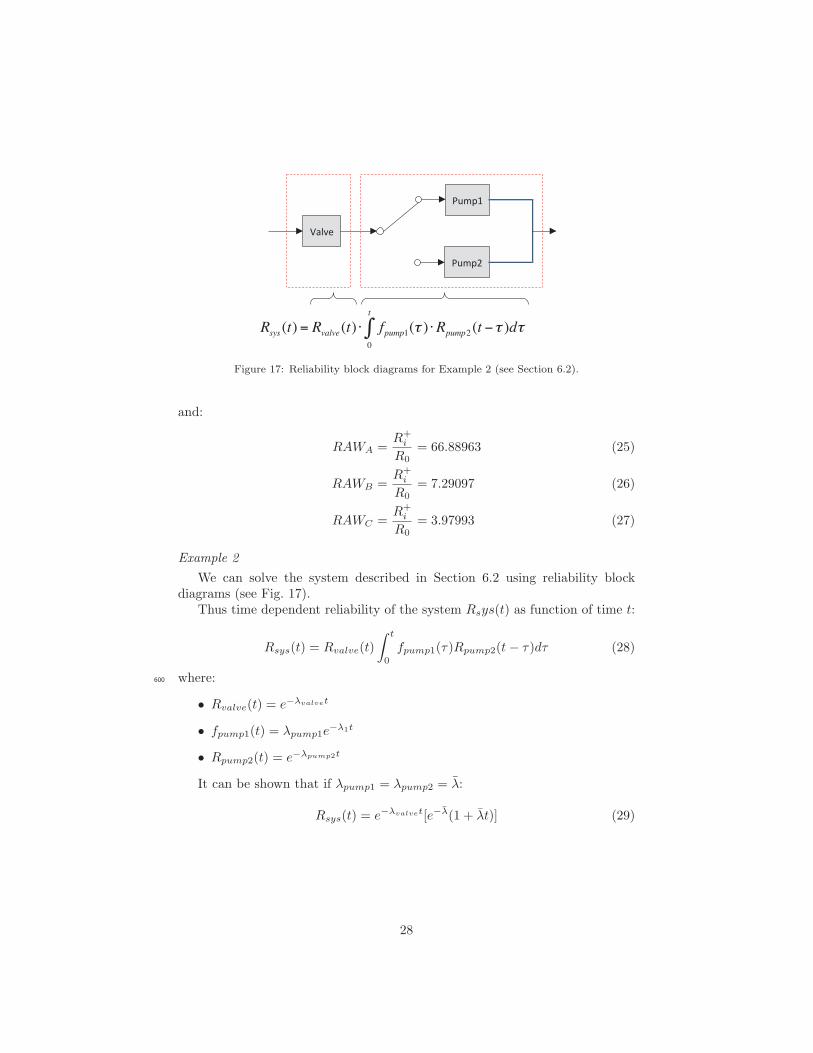
Rsys (t) = Rvalve(t) ⋅ fpump1(τ )0
t
∫ ⋅Rpump2 (t −τ )dτ
Figure 17: Reliability block diagrams for Example 2 (see Section 6.2).
and:
RAWA =R+
i
R0= 66.88963 (25)
RAWB =R+
i
R0= 7.29097 (26)
RAWC =R+
i
R0= 3.97993 (27)
Example 2
We can solve the system described in Section 6.2 using reliability blockdiagrams (see Fig. 17).
Thus time dependent reliability of the system Rsys(t) as function of time t:
Rsys(t) = Rvalve(t)
∫ t
0
fpump1(τ)Rpump2(t− τ)dτ (28)
where:600
• Rvalve(t) = e−λvalvet
• fpump1(t) = λpump1e−λ1t
• Rpump2(t) = e−λpump2t
It can be shown that if λpump1 = λpump2 = λ̄:
Rsys(t) = e−λvalvet[e−λ̄(1 + λ̄t)] (29)
28
For this system we have the following for a mission time T = 24 hours:
R0 = 1.0−Rsys(T ) = 0.85063876 (30)
R−valve = 1.0− [e−λ̄T (1 + λ̄T )] = 0.593994129 (31)
R+valve = 1.0 (32)
R−pump1 = 1.0−Rvalve(T ) = 0.6321205 (33)
R+pump1 = 1.0−Rvalve(T )Rpump2(T ) = 0.95021292 (34)
R−pump2 = R−
pump1 = 0.6321205 (35)
R+pump2 = R+
pump1 = 0.95021292 (36)
Example 3
We can solve the system described in Section 6.2 using again reliability blockdiagrams. Thus time dependent reliability of the system Rsys(t) as function oftime t:
Rsys(t) = Rvalve(t)R2oo3(t) (37)
where R2oo3(t) represents reliability of a set of three identical components in a605
2 out of 3 (2oo3) configuration.It can be shown that if λpump1 = λpump2 = λpump3 = λ̄ (thus Rpump1(t) =
Rpump2(t) = Rpump3(t) = R̄(t) = e−λ̄t) then R2oo3(t) can be written as
R2oo3(t) =
3∑n=2
(3
n
)R̄(t)n[1− R̄(t)]3−n = 3e−2λ̄t(1− e−λ̄t) + e−3λ̄t (38)
For this system we have the following for a mission time T = 24 hours:
R0 = 1.0−Rsys(T ) = 0.981609917 (39)
R−valve = 1.0−R2oo3(T ) = 0.95001058 (40)
R+valve = 1.0 (41)
R−pump1 = 1.0−R1oo2(T )Rvalve(T ) = 0.907163789 (42)
R+pump1 = 1.0−Rvalve(T )R̄(t)2 = 0.993262051 (43)
R−pump2 = R−
pump1 (44)
R+pump2 = R+
pump1 (45)
R−pump3 = R−
pump1 (46)
R+pump3 = R+
pump1 (47)
where R1oo2(t) represents reliability of a set of two identical components in a 1out of 2 (1oo2) configuration:
R1oo2(t) =
2∑n=1
(2
n
)R̄(t)n[1− R̄(t)]2−n = 2e−λ̄t(1− e−λ̄t) + e−2λ̄t (48)
29
References
[1] W. E. Vesely, T. C. Davis, R. S. Denning, N. Saltos, NUREC/CR-3385:610
Measures of Risk Importance and their Applications, Technical Report,U.S. Nuclear Regulatory Commission, Washington DC, 2005.
[2] K. Fleming, Developing useful insights and avoiding misleading conclu-sions from risk importance measures in PSA application, in: Proceedingsof PSA 1996 International Topical Meeting On Probabilistic Safety Assess-615
ment And Analysis, 1996.
[3] U. S. NRC, NUREC/CR-1150: Severe Accident Risks: An Assessment ForFive U.S. Nuclear Power Plants Final Summary Report, Technical Report,U.S. Nuclear Regulatory Commission, Washington DC, 2005.
[4] U. S. NRC, 10CFR50.69, Risk-Informed Categorization and Treatment of620
Structures, Systems and Components for Nuclear Power Reactors, Techni-cal Report, U.S. Nuclear Regulatory Commission, Washington DC, 2004.
[5] J. Devooght, C. Smidts, Probabilistic dynamics as a tool for dynamic PSA,Reliability Engineering & System Safety 52 (1996) 185 – 196.
[6] C. Rabiti, A. Alfonsi, J. Cogliati, D. Mandelli, R. Kinoshita, RAVEN, a625
new software for dynamic risk analysis, in: Proceedings of the ProbabilisticSafety Assessment andnd Management (PSAM) 12, 2014.
[7] B. Rutt, U. Catalyurek, A. Hakobyan, K. Metzroth, T. Aldemir, R. Den-ning, S. Dunagan, D. Kunsman, Distributed dynamic event tree generationfor reliability and risk assessment, in: 2006 IEEE Challenges of Large Ap-630
plications in Distributed Environments, 2006, pp. 61–70.
[8] K. S. Hsueh, A. Mosleh, The development and application of the acci-dent dynamic simulator for dynamic probabilistic risk assessment of nuclearpower plants, Reliability Engineering & System Safety 52 (1996) 297–314.
[9] E. Hofer, M. Kloos, B. Krzykacz-Hausmann, J. Peschke, M. Woltereck,635
An approximate epistemic uncertainty analysis approach in the presenceof epistemic and aleatory uncertainties, Reliability Engineering & SystemSafety 77 (2002) 229–238.
[10] R. C. D. Team, RELAP5-3D Code Manual, Technical Report, Idaho Na-tional Laboratory Technical Report, 2005.640
[11] R. O. Gauntt, MELCOR Computer Code Manual, Version 1.8.5, Vol. 2,Rev. 2, Sandia National Laboratories, NUREG/CR-6119, 2000.
[12] EPRI, Modular Accident Analysis Program 5 (MAAP5) Applications Guid-ance: Desktop Reference for Using MAAP5 Software - Phase 2 Report,Technical Report, Electric Power Reserach Institute, Palo Alto (CA), 2013.645
30
[13] C. Smith, C. Rabiti, R. Martineau, Risk Informed Safety Margins Charac-terization (RISMC) Pathway Technical Program Plan, Technical Report,Idaho National Laboratory Technical Report: INL/EXT-11-22977, 2011.
[14] D. Mandelli, C. Smith, T. Riley, J. Nielsen, A. Alfonsi, J. Cogliati, C. Ra-biti, J. Schroeder, BWR station blackout: A RISMC analysis using RAVEN650
and RELAP5-3D, Nuclear Technology 193 (2016) 161–174.
[15] D. Maljovec, S. Liu, B. Wang, D. Mandelli, P. T. Bremer, V. Pascucci,C. Smith, Analyzing simulation-based PRA data through traditional andtopological clustering: A BWR station blackout case study, ReliabilityEngineering & System Safety 145 (2015) 262–276.655
[16] D. Mandelli, S. Prescott, C. Smith, A. Alfonsi, C. Rabiti, J. Cogliati, R. Ki-noshita, Modeling of a flooding induced station blackout for a pressurizedwater reactor using the RISMC toolkit, in: Proceedings of PSA 2015 Inter-national Topical Meeting On Probabilistic Safety Assessment And Analysis,2015.660
[17] R. L. Boring, R. B. Shirley, J. C. Joe, D. Mandelli, C. Smith, SimulationAnd Non-Simulation Based Human Reliability Analysis Approaches, Tech-nical Report, Idaho National Laboratory Technical Report: INL/EXT-14-33903, 2014.
[18] H. S. Abdel-Khalik, Y. Bang, J. M. Hite, C. B. Kennedy, C. Wang, Re-665
duced order modeling for nonlinear multi-component models, InternationalJournal On Uncertainty Quantification (2012) 341–36.
[19] A. Alfonsi, C. Rabiti, D. Mandelli, J. Cogliati, R. Kinoshita, A. Naviglio,RAVEN and dynamic probabilistic risk assessment: Software overview, in:Proceedings of European Safety and Reliability Conference (ESREL 2014),670
Wroklaw (Poland), 2014.
[20] E. Zio, M. Marseguerra, J. Devooght, P. Labeau, A concept paper on dy-namic reliability via monte carlo simulation, Mathematics And ComputersIn Simulation 47 (1998) 371–382.
[21] J. C. Helton, F. J. Davis, Latin hypercube sampling and the propagation675
of uncertainty in analyses of complex systems, Reliability Engineering &System Safety 81 (2003).
[22] A. Amendola, G. Reina, DYLAM-1, a software package for event sequenceand consequence spectrum methodology, in: EUR-924, CEC-JRC. ISPRA:Commission of the European Communities, 1984.680
[23] G. Cojazzi, The DYLAM approach for the dynamic reliability analysis ofsystems, Reliability Engineering and System Safety 52 (1996) 279–296.
31
[24] C. Rabiti, D. Mandelli, A. Alfonsi, J. Cogliati, R. Kinoshita, Introductionof supervised learning capabilities of the RAVEN code for limit surfaceanalysis, in: Proceedings of American Nuclear Society (ANS), Reno (NV),685
2014.
[25] D. Mandelli, C. Smith, Adaptive sampling using support vector machines,in: Proceeding of American Nuclear Society (ANS), San Diego (CA), vol-ume 107, 2012, pp. 736–738.
[26] A. Alfonsi, C. Rabiti, D. Mandelli, J. Cogliati, R. Kinoshita, Adaptive690
dynamic event tree in RAVEN code, in: Proceedings of American NuclearSociety (ANS), Anaheim (CA), 2014.
[27] A. Alfonsi, C. Rabiti, D. Mandelli, J. Cogliati, R. Kinoshita, A. Naviglio,Dynamic event tree analysis through RAVEN, in: Proceedings of PSA2013 International Topical Meeting on Probabilistic Safety Assessment and695
Analysis Columbia, SC, on CD-ROM, American Nuclear Society, LaGrangePark, IL, 2013.
32

22
D. Mandelli, C. Parisi, Z. Ma, D. Maljovec, A. Alfonsi, C. Smith, “Measuring Risk-Importance in a Simulation-Based PRA Framework - Part II: Comparison Between Simulation-Based and Classical PRA Methods”, Draft for Reliability Engineering and System Safety.
Measuring Risk-Importance in a Simulation-BasedPRA Framework - Part II: Comparison with Classical
PRA Methods
D. Mandelli, C. Parisi, Z. Ma, D. Maljovec, C. Smith
Idaho National Laboratory (INL), 2525 Fremont Ave, 83402 Idaho Falls (ID), USA
Abstract
In the past decade several advanced Dynamic Probabilistic Risk Analysis (PRA)methods have been developed. These methods couple stochastic methods (e.g.,RAVEN, ADAPT, ADS, MCDET) with safety analysis codes (e.g., RELAP5-3D, MELCOR, MAAP) to determine risk associated to complex systems such asnuclear plants. Compared to classical PRA methods, which are based on staticBoolean logic structures (e.g., Event-Trees -ET-, Fault-Trees -FT-), they candetermine risk associated to complex systems with higher resolution since theimplicitly model timing and sequencing of events on the accident progression. Inthe first part of this article we have presented a set of risk importance measuresthat can be employed on a dataset generated by any Dynamic PRA methodto rank components based on their importance from a safety point of view.Such measures have been developed as a natural extension of ones employed inindustry PRA codes and they have been tested on several analytical test cases.In this second part of the article we show a full comparison between classicaland Dynamic PRA methods. The system considered for the comparison is aPressurized Water Reactor (PWR) system for a large break Loss Of CoolantAccident (LOCA) initiating event. We show how the Dynamic and the ET/FTmodels have been built from both a stochastic and accident progression point ofview. Metrics of comparison are based not only on the core damage probabilitybut also based on the importance values associated to each basic event.
Keywords: Importance Measures, Dynamic PRA, Probabilistic RiskAssessment
1. Introduction
In the past decades, several numerical simulation codes have been employedto simulate accident dynamics, e.g., RELAP5-3D [1], MELCOR [2] or MAAP [3].In order to evaluate the impact of uncertainties into accident dynamics, severalstochastic methodologies have been coupled with these codes. These stochas-5
tic methods range from classical Monte-Carlo and Latin Hypercube samplingto stochastic polynomial methods. Similar approaches have been introduced
Preprint submitted to Reliability Engineering & System Safety September 30, 2017
into the risk and safety community where stochastic methods, e.g., RAVEN [4],ADAPT [5], MCDET [6] or ADS [7], have been coupled with safety analysiscodes in order to evaluate the safety impact of timing and sequencing of events10
on the accident progression. These approaches are usually called Dynamic PRAmethods [8].
Compared to classical PRA methods, which are based on static Booleanlogic structures (e.g., Event-Trees -ET-, Fault-Trees -FT-), they can determinerisk associated to complex systems with higher resolution since the implicitly15
model timing and sequencing of events on the accident progression. In ET/FTbased methods accident progression is fixed and it is set prior the analysis bythe analyst. Such approximation is even more limiting for accident scenariosin which tight timing dependencies of events are coupled with plant dynamics(e.g., recovery actions and human related actions).20
The scope of this paper is to present a comparison between Dynamic andclassical PRA methods. The system considered is a Pressurized Water Rec-tor (PWR) for a large break Loss Of Coolant Accident (LOCA), LB-LOCA,initiating event.
The comparison Dynamic and classical PRA methods is based not only on25
the core damage probability but also based on the importance values associatedto each basic event.
In [9] we have presented a set of risk importance measures that can beemployed on a dataset generated by any Dynamic PRA method to rank com-ponents based on their importance from a safety point of view. Such measures30
have been developed as a natural extension of the ones employed in industryPRA codes such SAPHIRE [10] or CAFTA [11].
In this paper we employs such metrics extensively in order to quantify suchcomparison. The objectives are twofold: the first one is to validate the proposedmetrics over an industry-grade test case and show capabilities of Dynamic PRA35
methods. The second one is to provide guidance on how it is possible to haveclassical and dynamic PRA methods compatible with each other. The rationalebehind it is that a Dynamic PRA analysis can be performed for a limited aspectof the overall system and its result incorporated into a classical PRA results.Similarly, a classical PRA analysis can be “made dynamic” by adding dynamic40
elements (e.g., quantitative information of timing of events) into it and coupledwith a system simulation code.
2. Test Case
The test case considered in this paper is a 3-loop PWR system of Westing-house design with a large-dry containment. The initiating event is a LB-LOCA:45
a double-ended guillotine break of one the three hot legs.Under these accident conditions, the system experiences a sudden sub-cooled
blowdown and primary system pressure drops from about 2200 psi down to thesaturation pressure (about 1000 psi).
2
In order to compensate the large loss of coolant inventory into the vessel50
and prevent core damage, two emergency core-cooling systems are employed:Accumulators and Low-Pressure Injection System (LPIS).
Accumulators are passive components consisting of pressurized water tanksthat are employed at the beginning of the transient and can dump large inven-tory of sub-cooled water into the vessel.55
The LPIS is activated when primary system pressure falls below 980 psi andby using pumps large amount of water are transfered from the Reactor WaterStorage Tank (RWST) directly into the vessel.
The large amount of water that leaves the primary system and is collected inthe containment and, thus, its temperature and pressure increases. In order to60
cool it down, Containment Sprays (CSs) are employed. Similarly to the LPIS,through pumps RWST water is sprayed from the top level of the containment.
Once RWST is empty, both CSs and LPISs switch from injection mode torecirculation mode: water collected at the base of the containment and throughthe sump and is injected back into the vessel (through the LPI) and into the65
containment (through the CSs).
3. Comparison Workflow
The comparison between Classical (using SAPHIRE) and Dynamic PRAanalysis (using RAVEN/RELAP5-3D) has been performed following these steps:
1. Simplify the SAPHIRE FT structure by grouping its basic events into70
macro basic events
2. Perform calculation of the ET-FT model: determine CD probability, prob-ability of each ET branch and the risk importance of each macro basicevents
3. Consider the SAPHIRE ET for the LLOCA initiating event and model75
the RELAP5-3D accident progression following consistently with the ETlogic.
4. Construct the PWR logic based on the same macro basic events deter-mined in Step 1: these macro basic events constitute the stochastic vari-ables sampled by RAVEN80
5. Perform a dynamic analysis using RAVEN/RELAP5-3D for the systemconstructed in Steps 4 and 5, and determine probability of each ET branchand the risk importance of each macro basic events
6. Compare the results obtained in Steps 3 and 5
Step 1 has been deemed necessary in order to limit the number of unnecessary85
RELAP5-3D simulation runs. The rationale is that each basic event in the setof FTs are also stochastic variables sampled by RAVEN. If all basic events areconsidered (about a hundred) then the sampling strategy would require a verylarge number of RELAP5-3D simulation runs. The great majority of these runswould be identical since the impact of these basic events on accident progression90
is the same.
3
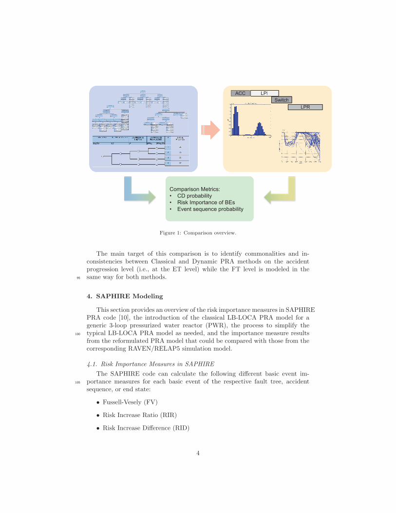
Figure 1: Comparison overview.
The main target of this comparison is to identify commonalities and in-consistencies between Classical and Dynamic PRA methods on the accidentprogression level (i.e., at the ET level) while the FT level is modeled in thesame way for both methods.95
4. SAPHIRE Modeling
This section provides an overview of the risk importance measures in SAPHIREPRA code [10], the introduction of the classical LB-LOCA PRA model for ageneric 3-loop pressurized water reactor (PWR), the process to simplify thetypical LB-LOCA PRA model as needed, and the importance measure results100
from the reformulated PRA model that could be compared with those from thecorresponding RAVEN/RELAP5 simulation model.
4.1. Risk Importance Measures in SAPHIRE
The SAPHIRE code can calculate the following different basic event im-portance measures for each basic event of the respective fault tree, accident105
sequence, or end state:
• Fussell-Vesely (FV)
• Risk Increase Ratio (RIR)
• Risk Increase Difference (RID)
4
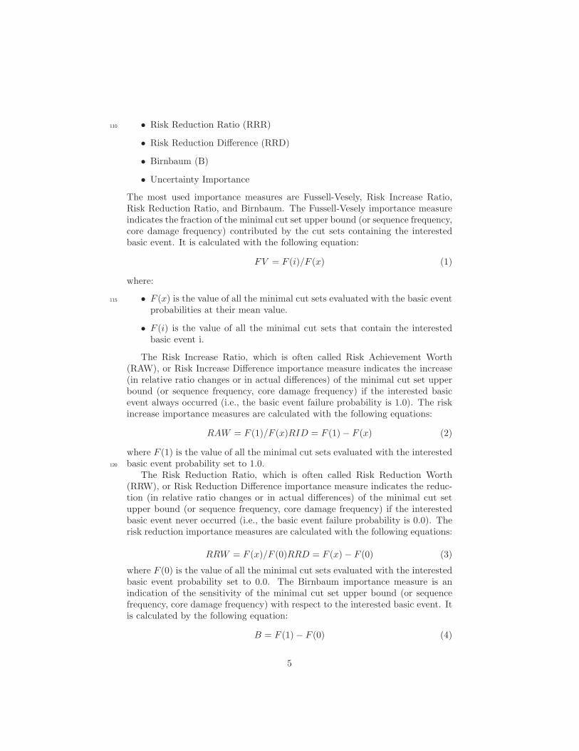
• Risk Reduction Ratio (RRR)110
• Risk Reduction Difference (RRD)
• Birnbaum (B)
• Uncertainty Importance
The most used importance measures are Fussell-Vesely, Risk Increase Ratio,Risk Reduction Ratio, and Birnbaum. The Fussell-Vesely importance measureindicates the fraction of the minimal cut set upper bound (or sequence frequency,core damage frequency) contributed by the cut sets containing the interestedbasic event. It is calculated with the following equation:
FV = F (i)/F (x) (1)
where:
• F (x) is the value of all the minimal cut sets evaluated with the basic event115
probabilities at their mean value.
• F (i) is the value of all the minimal cut sets that contain the interestedbasic event i.
The Risk Increase Ratio, which is often called Risk Achievement Worth(RAW), or Risk Increase Difference importance measure indicates the increase(in relative ratio changes or in actual differences) of the minimal cut set upperbound (or sequence frequency, core damage frequency) if the interested basicevent always occurred (i.e., the basic event failure probability is 1.0). The riskincrease importance measures are calculated with the following equations:
RAW = F (1)/F (x)RID = F (1)− F (x) (2)
where F (1) is the value of all the minimal cut sets evaluated with the interestedbasic event probability set to 1.0.120
The Risk Reduction Ratio, which is often called Risk Reduction Worth(RRW), or Risk Reduction Difference importance measure indicates the reduc-tion (in relative ratio changes or in actual differences) of the minimal cut setupper bound (or sequence frequency, core damage frequency) if the interestedbasic event never occurred (i.e., the basic event failure probability is 0.0). Therisk reduction importance measures are calculated with the following equations:
RRW = F (x)/F (0)RRD = F (x)− F (0) (3)
where F (0) is the value of all the minimal cut sets evaluated with the interestedbasic event probability set to 0.0. The Birnbaum importance measure is anindication of the sensitivity of the minimal cut set upper bound (or sequencefrequency, core damage frequency) with respect to the interested basic event. Itis calculated by the following equation:
B = F (1)− F (0) (4)
5
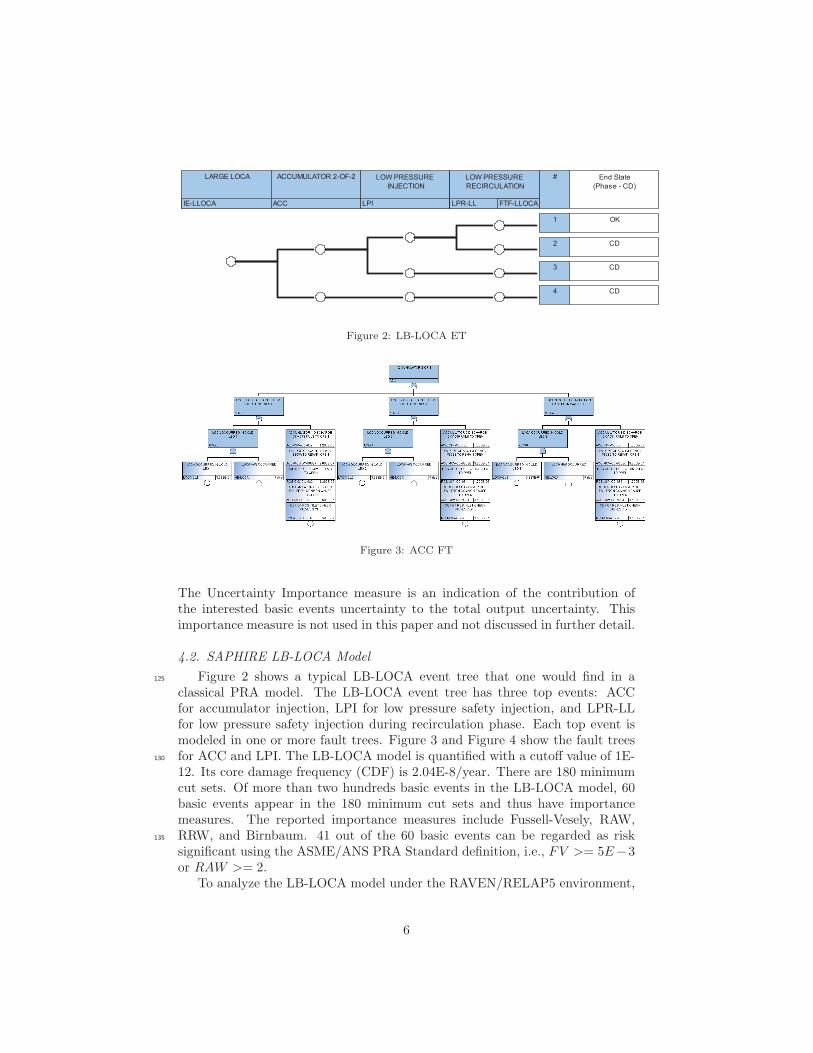
Figure 2: LB-LOCA ET
Figure 3: ACC FT
The Uncertainty Importance measure is an indication of the contribution ofthe interested basic events uncertainty to the total output uncertainty. Thisimportance measure is not used in this paper and not discussed in further detail.
4.2. SAPHIRE LB-LOCA Model
Figure 2 shows a typical LB-LOCA event tree that one would find in a125
classical PRA model. The LB-LOCA event tree has three top events: ACCfor accumulator injection, LPI for low pressure safety injection, and LPR-LLfor low pressure safety injection during recirculation phase. Each top event ismodeled in one or more fault trees. Figure 3 and Figure 4 show the fault treesfor ACC and LPI. The LB-LOCA model is quantified with a cutoff value of 1E-130
12. Its core damage frequency (CDF) is 2.04E-8/year. There are 180 minimumcut sets. Of more than two hundreds basic events in the LB-LOCA model, 60basic events appear in the 180 minimum cut sets and thus have importancemeasures. The reported importance measures include Fussell-Vesely, RAW,RRW, and Birnbaum. 41 out of the 60 basic events can be regarded as risk135
significant using the ASME/ANS PRA Standard definition, i.e., FV >= 5E−3or RAW >= 2.
To analyze the LB-LOCA model under the RAVEN/RELAP5 environment,
6
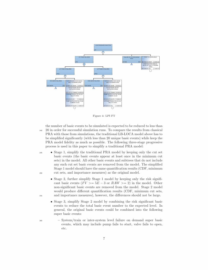
Figure 4: LPI FT
the number of basic events to be simulated is expected to be reduced to less than20 in order for successful simulation runs. To compare the results from classical140
PRA with those from simulations, the traditional LB-LOCA model above has tobe simplified significantly (with less than 20 unique basic events) while keep thePRA model fidelity as much as possible. The following three-stage progressiveprocess is used in this paper to simplify a traditional PRA model:
• Stage 1, simplify the traditional PRA model by keeping only the cut set145
basic events (the basic events appear at least once in the minimum cutsets) in the model. All other basic events and subtrees that do not includeany such cut set basic events are removed from the model. The simplifiedStage 1 model should have the same quantification results (CDF, minimumcut sets, and importance measures) as the original model.150
• Stage 2, further simplify Stage 1 model by keeping only the risk signifi-cant basic events (FV >= 5E − 3 or RAW >= 2) in the model. Othernon-significant basic events are removed from the model. Stage 2 modelwould produce different quantification results (CDF, minimum cut sets,and importance measures), however, the differences should not be large.155
• Stage 3, simplify Stage 2 model by combining the risk significant basicevents to reduce the total basic event number to the expected level. Ingeneral, the original basic events could be combined into the followingsuper basic events:
– System/train or inter-system level failure on demand super basic160
events, which may include pump fails to start, valve fails to open,etc.
7
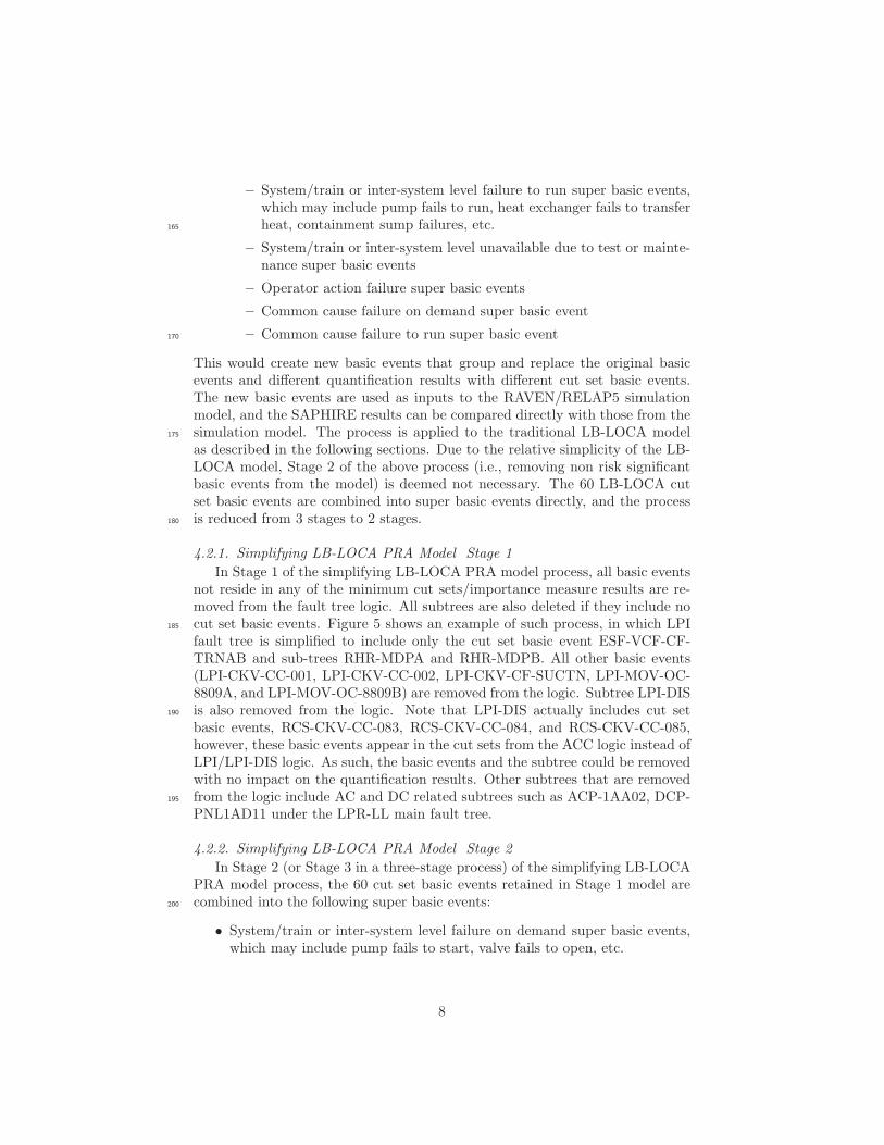
– System/train or inter-system level failure to run super basic events,which may include pump fails to run, heat exchanger fails to transferheat, containment sump failures, etc.165
– System/train or inter-system level unavailable due to test or mainte-nance super basic events
– Operator action failure super basic events
– Common cause failure on demand super basic event
– Common cause failure to run super basic event170
This would create new basic events that group and replace the original basicevents and different quantification results with different cut set basic events.The new basic events are used as inputs to the RAVEN/RELAP5 simulationmodel, and the SAPHIRE results can be compared directly with those from thesimulation model. The process is applied to the traditional LB-LOCA model175
as described in the following sections. Due to the relative simplicity of the LB-LOCA model, Stage 2 of the above process (i.e., removing non risk significantbasic events from the model) is deemed not necessary. The 60 LB-LOCA cutset basic events are combined into super basic events directly, and the processis reduced from 3 stages to 2 stages.180
4.2.1. Simplifying LB-LOCA PRA Model Stage 1
In Stage 1 of the simplifying LB-LOCA PRA model process, all basic eventsnot reside in any of the minimum cut sets/importance measure results are re-moved from the fault tree logic. All subtrees are also deleted if they include nocut set basic events. Figure 5 shows an example of such process, in which LPI185
fault tree is simplified to include only the cut set basic event ESF-VCF-CF-TRNAB and sub-trees RHR-MDPA and RHR-MDPB. All other basic events(LPI-CKV-CC-001, LPI-CKV-CC-002, LPI-CKV-CF-SUCTN, LPI-MOV-OC-8809A, and LPI-MOV-OC-8809B) are removed from the logic. Subtree LPI-DISis also removed from the logic. Note that LPI-DIS actually includes cut set190
basic events, RCS-CKV-CC-083, RCS-CKV-CC-084, and RCS-CKV-CC-085,however, these basic events appear in the cut sets from the ACC logic instead ofLPI/LPI-DIS logic. As such, the basic events and the subtree could be removedwith no impact on the quantification results. Other subtrees that are removedfrom the logic include AC and DC related subtrees such as ACP-1AA02, DCP-195
PNL1AD11 under the LPR-LL main fault tree.
4.2.2. Simplifying LB-LOCA PRA Model Stage 2
In Stage 2 (or Stage 3 in a three-stage process) of the simplifying LB-LOCAPRA model process, the 60 cut set basic events retained in Stage 1 model arecombined into the following super basic events:200
• System/train or inter-system level failure on demand super basic events,which may include pump fails to start, valve fails to open, etc.
8
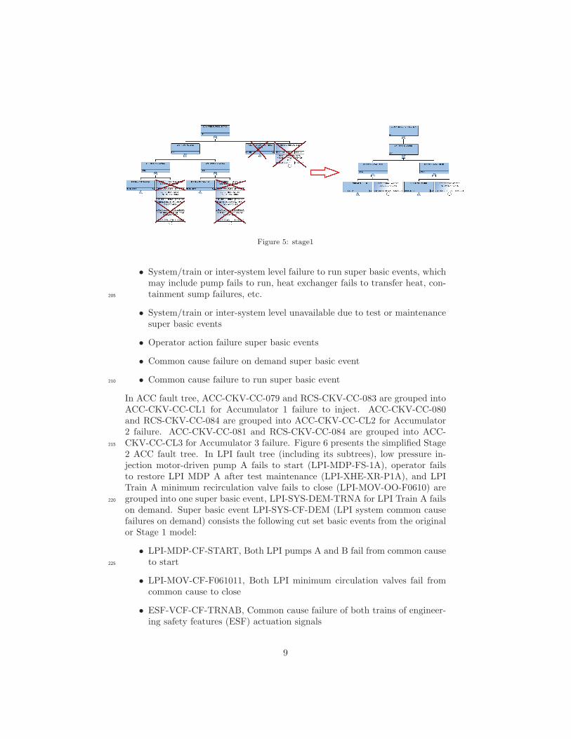
Figure 5: stage1
• System/train or inter-system level failure to run super basic events, whichmay include pump fails to run, heat exchanger fails to transfer heat, con-tainment sump failures, etc.205
• System/train or inter-system level unavailable due to test or maintenancesuper basic events
• Operator action failure super basic events
• Common cause failure on demand super basic event
• Common cause failure to run super basic event210
In ACC fault tree, ACC-CKV-CC-079 and RCS-CKV-CC-083 are grouped intoACC-CKV-CC-CL1 for Accumulator 1 failure to inject. ACC-CKV-CC-080and RCS-CKV-CC-084 are grouped into ACC-CKV-CC-CL2 for Accumulator2 failure. ACC-CKV-CC-081 and RCS-CKV-CC-084 are grouped into ACC-CKV-CC-CL3 for Accumulator 3 failure. Figure 6 presents the simplified Stage215
2 ACC fault tree. In LPI fault tree (including its subtrees), low pressure in-jection motor-driven pump A fails to start (LPI-MDP-FS-1A), operator failsto restore LPI MDP A after test maintenance (LPI-XHE-XR-P1A), and LPITrain A minimum recirculation valve fails to close (LPI-MOV-OO-F0610) aregrouped into one super basic event, LPI-SYS-DEM-TRNA for LPI Train A fails220
on demand. Super basic event LPI-SYS-CF-DEM (LPI system common causefailures on demand) consists the following cut set basic events from the originalor Stage 1 model:
• LPI-MDP-CF-START, Both LPI pumps A and B fail from common causeto start225
• LPI-MOV-CF-F061011, Both LPI minimum circulation valves fail fromcommon cause to close
• ESF-VCF-CF-TRNAB, Common cause failure of both trains of engineer-ing safety features (ESF) actuation signals
9
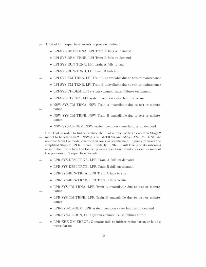
A list of LPI super basic events is provided below:230
• LPI-SYS-DEM-TRNA, LPI Train A fails on demand
• LPI-SYS-DEM-TRNB, LPI Train B fails on demand
• LPI-SYS-RUN-TRNA, LPI Train A fails to run
• LPI-SYS-RUN-TRNB, LPI Train B fails to run
• LPI-SYS-TM-TRNA, LPI Train A unavailable due to test or maintenance235
• LPI-SYS-TM-TRNB, LPI Train B unavailable due to test or maintenance
• LPI-SYS-CF-DEM, LPI system common cause failures on demand
• LPI-SYS-CF-RUN, LPI system common cause failures to run
• NSW-SYS-TM-TRNA, NSW Train A unavailable due to test or mainte-nance240
• NSW-SYS-TM-TRNB, NSW Train B unavailable due to test or mainte-nance
• NSW-SYS-CF-DEM, NSW system common cause failures on demand
Note that in order to further reduce the final number of basic events in Stage 2model to be less than 20, NSW-SYS-TM-TRNA and NSW-SYS-TM-TRNB are245
removed from the model due to their low risk significance. Figure 7 presents thesimplified Stage 2 LPI fault tree. Similarly, LPR-LL fault tree (and its subtrees)is simplified to include the following new super basic events, as well as some ofthe previous LPI super basic events:
• LPR-SYS-DEM-TRNA, LPR Train A fails on demand250
• LPR-SYS-DEM-TRNB, LPR Train B fails on demand
• LPR-SYS-RUN-TRNA, LPR Train A fails to run
• LPR-SYS-RUN-TRNB, LPR Train B fails to run
• LPR-SYS-TM-TRNA, LPR Train A unavailable due to test or mainte-nance255
• LPR-SYS-TM-TRNB, LPR Train B unavailable due to test or mainte-nance
• LPR-SYS-CF-DEM, LPR system common cause failures on demand
• LPR-SYS-CF-RUN, LPR system common cause failures to run
• LPR-XHE-XM-ERROR, Operator fails to initiate recirculation or hot leg260
recirculation
10
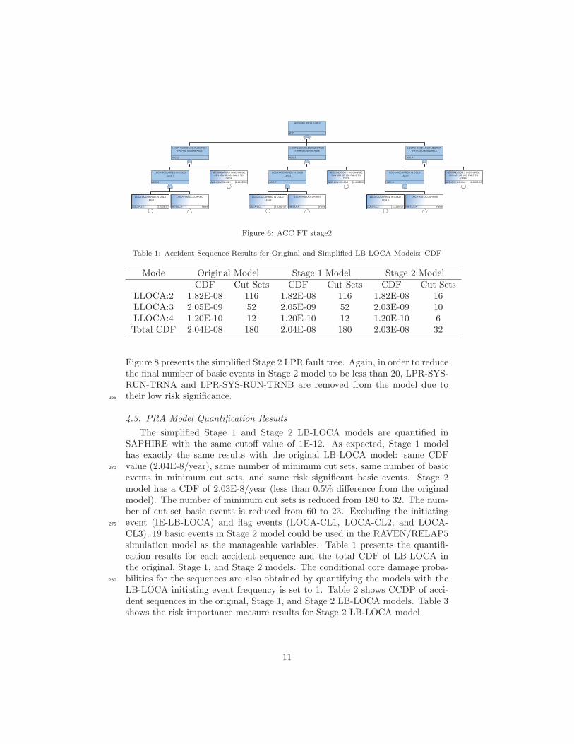
Figure 6: ACC FT stage2
Table 1: Accident Sequence Results for Original and Simplified LB-LOCA Models: CDF
Mode Original Model Stage 1 Model Stage 2 ModelCDF Cut Sets CDF Cut Sets CDF Cut Sets
LLOCA:2 1.82E-08 116 1.82E-08 116 1.82E-08 16LLOCA:3 2.05E-09 52 2.05E-09 52 2.03E-09 10LLOCA:4 1.20E-10 12 1.20E-10 12 1.20E-10 6Total CDF 2.04E-08 180 2.04E-08 180 2.03E-08 32
Figure 8 presents the simplified Stage 2 LPR fault tree. Again, in order to reducethe final number of basic events in Stage 2 model to be less than 20, LPR-SYS-RUN-TRNA and LPR-SYS-RUN-TRNB are removed from the model due totheir low risk significance.265
4.3. PRA Model Quantification Results
The simplified Stage 1 and Stage 2 LB-LOCA models are quantified inSAPHIRE with the same cutoff value of 1E-12. As expected, Stage 1 modelhas exactly the same results with the original LB-LOCA model: same CDFvalue (2.04E-8/year), same number of minimum cut sets, same number of basic270
events in minimum cut sets, and same risk significant basic events. Stage 2model has a CDF of 2.03E-8/year (less than 0.5% difference from the originalmodel). The number of minimum cut sets is reduced from 180 to 32. The num-ber of cut set basic events is reduced from 60 to 23. Excluding the initiatingevent (IE-LB-LOCA) and flag events (LOCA-CL1, LOCA-CL2, and LOCA-275
CL3), 19 basic events in Stage 2 model could be used in the RAVEN/RELAP5simulation model as the manageable variables. Table 1 presents the quantifi-cation results for each accident sequence and the total CDF of LB-LOCA inthe original, Stage 1, and Stage 2 models. The conditional core damage proba-bilities for the sequences are also obtained by quantifying the models with the280
LB-LOCA initiating event frequency is set to 1. Table 2 shows CCDP of acci-dent sequences in the original, Stage 1, and Stage 2 LB-LOCA models. Table 3shows the risk importance measure results for Stage 2 LB-LOCA model.
11
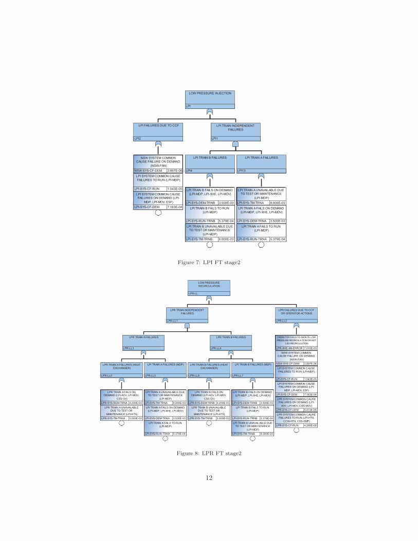
Figure 7: LPI FT stage2
Figure 8: LPR FT stage2
12
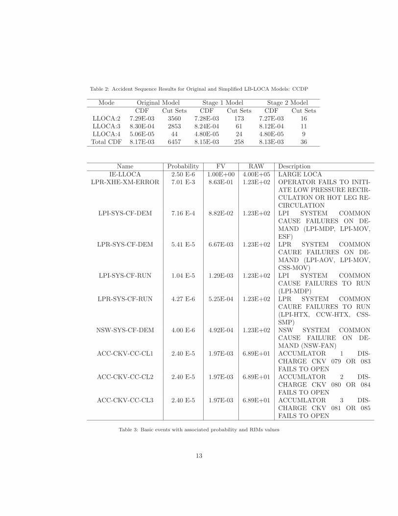
Table 2: Accident Sequence Results for Original and Simplified LB-LOCA Models: CCDP
Mode Original Model Stage 1 Model Stage 2 ModelCDF Cut Sets CDF Cut Sets CDF Cut Sets
LLOCA:2 7.29E-03 3560 7.28E-03 173 7.27E-03 16LLOCA:3 8.30E-04 2853 8.24E-04 61 8.12E-04 11LLOCA:4 5.06E-05 44 4.80E-05 24 4.80E-05 9Total CDF 8.17E-03 6457 8.15E-03 258 8.13E-03 36
Name Probability FV RAW DescriptionIE-LLOCA 2.50 E-6 1.00E+00 4.00E+05 LARGE LOCA
LPR-XHE-XM-ERROR 7.01 E-3 8.63E-01 1.23E+02 OPERATOR FAILS TO INITI-ATE LOW PRESSURE RECIR-CULATION OR HOT LEG RE-CIRCULATION
LPI-SYS-CF-DEM 7.16 E-4 8.82E-02 1.23E+02 LPI SYSTEM COMMONCAUSE FAILURES ON DE-MAND (LPI-MDP, LPI-MOV,ESF)
LPR-SYS-CF-DEM 5.41 E-5 6.67E-03 1.23E+02 LPR SYSTEM COMMONCAURE FAILURES ON DE-MAND (LPI-AOV, LPI-MOV,CSS-MOV)
LPI-SYS-CF-RUN 1.04 E-5 1.29E-03 1.23E+02 LPI SYSTEM COMMONCAUSE FAILURES TO RUN(LPI-MDP)
LPR-SYS-CF-RUN 4.27 E-6 5.25E-04 1.23E+02 LPR SYSTEM COMMONCAURE FAILURES TO RUN(LPI-HTX, CCW-HTX, CSS-SMP)
NSW-SYS-CF-DEM 4.00 E-6 4.92E-04 1.23E+02 NSW SYSTEM COMMONCAUSE FAILURE ON DE-MAND (NSW-FAN)
ACC-CKV-CC-CL1 2.40 E-5 1.97E-03 6.89E+01 ACCUMLATOR 1 DIS-CHARGE CKV 079 OR 083FAILS TO OPEN
ACC-CKV-CC-CL2 2.40 E-5 1.97E-03 6.89E+01 ACCUMLATOR 2 DIS-CHARGE CKV 080 OR 084FAILS TO OPEN
ACC-CKV-CC-CL3 2.40 E-5 1.97E-03 6.89E+01 ACCUMLATOR 3 DIS-CHARGE CKV 081 OR 085FAILS TO OPEN
Table 3: Basic events with associated probability and RIMs values
13
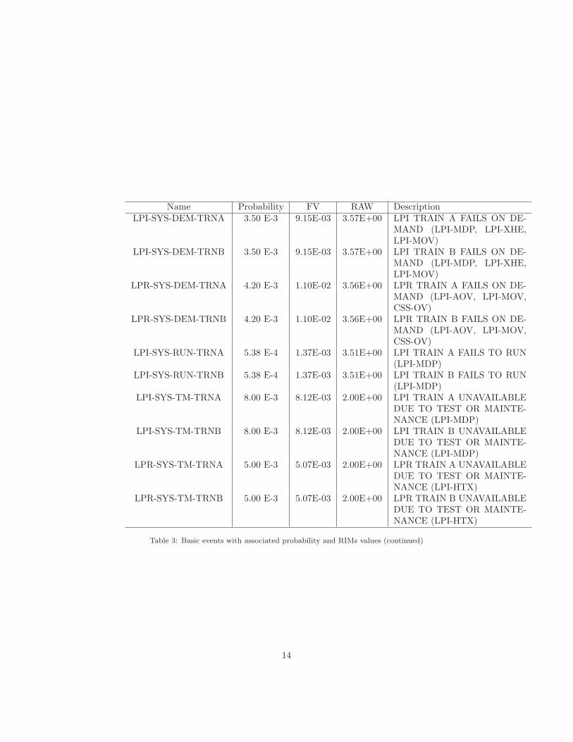
Name Probability FV RAW DescriptionLPI-SYS-DEM-TRNA 3.50 E-3 9.15E-03 3.57E+00 LPI TRAIN A FAILS ON DE-
MAND (LPI-MDP, LPI-XHE,LPI-MOV)
LPI-SYS-DEM-TRNB 3.50 E-3 9.15E-03 3.57E+00 LPI TRAIN B FAILS ON DE-MAND (LPI-MDP, LPI-XHE,LPI-MOV)
LPR-SYS-DEM-TRNA 4.20 E-3 1.10E-02 3.56E+00 LPR TRAIN A FAILS ON DE-MAND (LPI-AOV, LPI-MOV,CSS-OV)
LPR-SYS-DEM-TRNB 4.20 E-3 1.10E-02 3.56E+00 LPR TRAIN B FAILS ON DE-MAND (LPI-AOV, LPI-MOV,CSS-OV)
LPI-SYS-RUN-TRNA 5.38 E-4 1.37E-03 3.51E+00 LPI TRAIN A FAILS TO RUN(LPI-MDP)
LPI-SYS-RUN-TRNB 5.38 E-4 1.37E-03 3.51E+00 LPI TRAIN B FAILS TO RUN(LPI-MDP)
LPI-SYS-TM-TRNA 8.00 E-3 8.12E-03 2.00E+00 LPI TRAIN A UNAVAILABLEDUE TO TEST OR MAINTE-NANCE (LPI-MDP)
LPI-SYS-TM-TRNB 8.00 E-3 8.12E-03 2.00E+00 LPI TRAIN B UNAVAILABLEDUE TO TEST OR MAINTE-NANCE (LPI-MDP)
LPR-SYS-TM-TRNA 5.00 E-3 5.07E-03 2.00E+00 LPR TRAIN A UNAVAILABLEDUE TO TEST OR MAINTE-NANCE (LPI-HTX)
LPR-SYS-TM-TRNB 5.00 E-3 5.07E-03 2.00E+00 LPR TRAIN B UNAVAILABLEDUE TO TEST OR MAINTE-NANCE (LPI-HTX)
Table 3: Basic events with associated probability and RIMs values (continued)
14
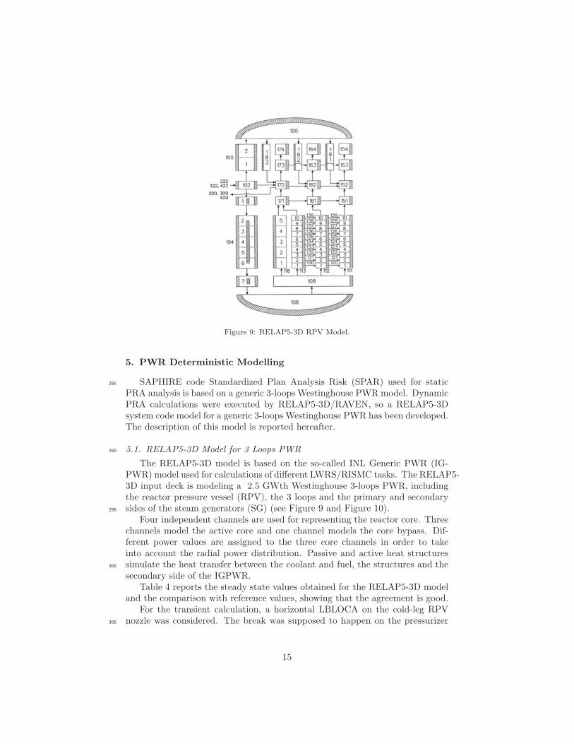
Figure 9: RELAP5-3D RPV Model.
5. PWR Deterministic Modelling
SAPHIRE code Standardized Plan Analysis Risk (SPAR) used for static285
PRA analysis is based on a generic 3-loops Westinghouse PWR model. DynamicPRA calculations were executed by RELAP5-3D/RAVEN, so a RELAP5-3Dsystem code model for a generic 3-loops Westinghouse PWR has been developed.The description of this model is reported hereafter.
5.1. RELAP5-3D Model for 3 Loops PWR290
The RELAP5-3D model is based on the so-called INL Generic PWR (IG-PWR) model used for calculations of different LWRS/RISMC tasks. The RELAP5-3D input deck is modeling a 2.5 GWth Westinghouse 3-loops PWR, includingthe reactor pressure vessel (RPV), the 3 loops and the primary and secondarysides of the steam generators (SG) (see Figure 9 and Figure 10).295
Four independent channels are used for representing the reactor core. Threechannels model the active core and one channel models the core bypass. Dif-ferent power values are assigned to the three core channels in order to takeinto account the radial power distribution. Passive and active heat structuressimulate the heat transfer between the coolant and fuel, the structures and the300
secondary side of the IGPWR.Table 4 reports the steady state values obtained for the RELAP5-3D model
and the comparison with reference values, showing that the agreement is good.For the transient calculation, a horizontal LBLOCA on the cold-leg RPV
nozzle was considered. The break was supposed to happen on the pressurizer305
15
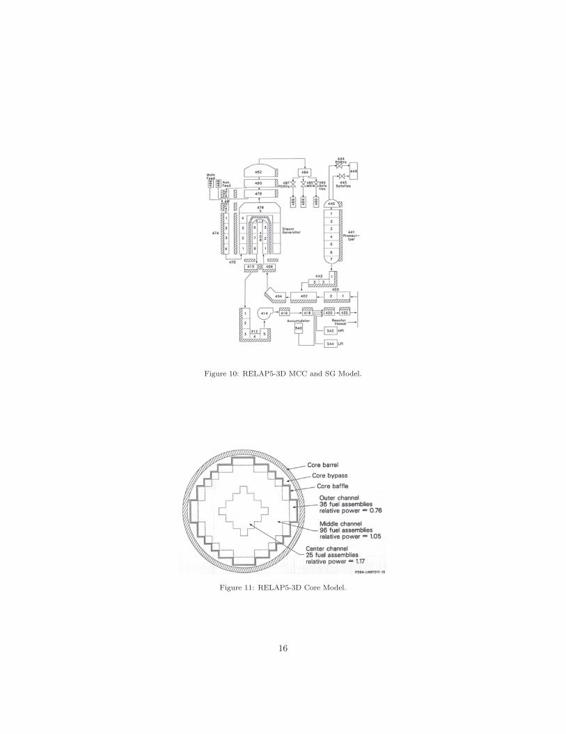
Figure 10: RELAP5-3D MCC and SG Model.
Figure 11: RELAP5-3D Core Model.
16
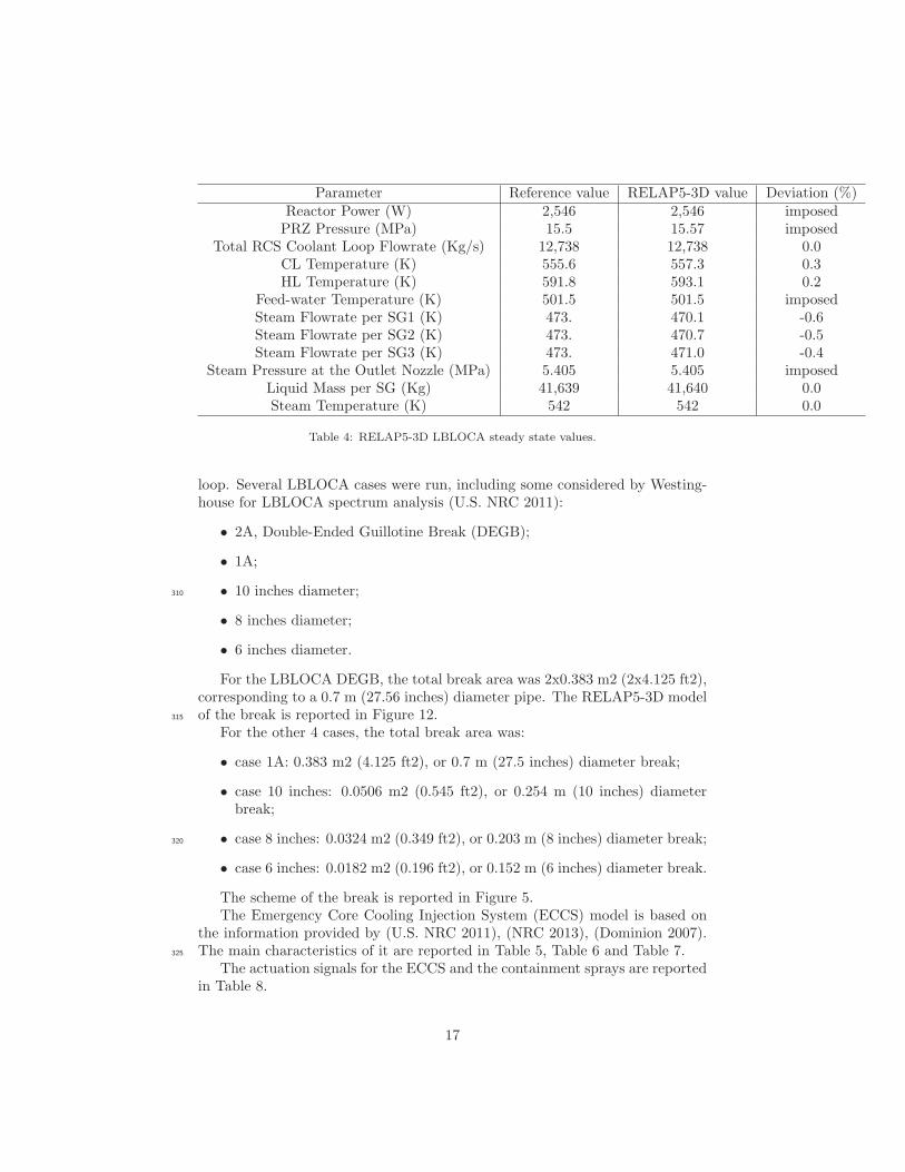
Parameter Reference value RELAP5-3D value Deviation (%)Reactor Power (W) 2,546 2,546 imposedPRZ Pressure (MPa) 15.5 15.57 imposed
Total RCS Coolant Loop Flowrate (Kg/s) 12,738 12,738 0.0CL Temperature (K) 555.6 557.3 0.3HL Temperature (K) 591.8 593.1 0.2
Feed-water Temperature (K) 501.5 501.5 imposedSteam Flowrate per SG1 (K) 473. 470.1 -0.6Steam Flowrate per SG2 (K) 473. 470.7 -0.5Steam Flowrate per SG3 (K) 473. 471.0 -0.4
Steam Pressure at the Outlet Nozzle (MPa) 5.405 5.405 imposedLiquid Mass per SG (Kg) 41,639 41,640 0.0Steam Temperature (K) 542 542 0.0
Table 4: RELAP5-3D LBLOCA steady state values.
loop. Several LBLOCA cases were run, including some considered by Westing-house for LBLOCA spectrum analysis (U.S. NRC 2011):
• 2A, Double-Ended Guillotine Break (DEGB);
• 1A;
• 10 inches diameter;310
• 8 inches diameter;
• 6 inches diameter.
For the LBLOCA DEGB, the total break area was 2x0.383 m2 (2x4.125 ft2),corresponding to a 0.7 m (27.56 inches) diameter pipe. The RELAP5-3D modelof the break is reported in Figure 12.315
For the other 4 cases, the total break area was:
• case 1A: 0.383 m2 (4.125 ft2), or 0.7 m (27.5 inches) diameter break;
• case 10 inches: 0.0506 m2 (0.545 ft2), or 0.254 m (10 inches) diameterbreak;
• case 8 inches: 0.0324 m2 (0.349 ft2), or 0.203 m (8 inches) diameter break;320
• case 6 inches: 0.0182 m2 (0.196 ft2), or 0.152 m (6 inches) diameter break.
The scheme of the break is reported in Figure 5.The Emergency Core Cooling Injection System (ECCS) model is based on
the information provided by (U.S. NRC 2011), (NRC 2013), (Dominion 2007).The main characteristics of it are reported in Table 5, Table 6 and Table 7.325
The actuation signals for the ECCS and the containment sprays are reportedin Table 8.
17
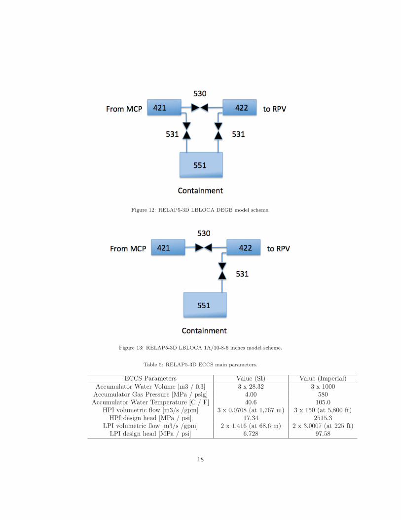
Figure 12: RELAP5-3D LBLOCA DEGB model scheme.
Figure 13: RELAP5-3D LBLOCA 1A/10-8-6 inches model scheme.
Table 5: RELAP5-3D ECCS main parameters.
ECCS Parameters Value (SI) Value (Imperial)Accumulator Water Volume [m3 / ft3] 3 x 28.32 3 x 1000Accumulator Gas Pressure [MPa / psig] 4.00 580Accumulator Water Temperature [C / F] 40.6 105.0
HPI volumetric flow [m3/s /gpm] 3 x 0.0708 (at 1,767 m) 3 x 150 (at 5,800 ft)HPI design head [MPa / psi] 17.34 2515.3
LPI volumetric flow [m3/s /gpm] 2 x 1.416 (at 68.6 m) 2 x 3,0007 (at 225 ft)LPI design head [MPa / psi] 6.728 97.58
18
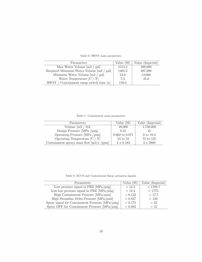
Table 6: RWST main parameters.
Parameters Value (SI) Value (Imperial)Max Water Volume [m3 / gal] 1514.2 400,000
Required Minimum Water Volume [m3 / gal] 1465.3 387,000Minimum Water Volume [m3 / gal] 53.0 14,000
Water Temperature [C / F] 7.2 45.0RWST / Containment sump switch time (s) 150.0
Table 7: Containment main parameters.
Parameters Value (SI) Value (Imperial)Volume [m3 / ft3] 49,000 1,730,000
Design Pressure [MPa /psig] 0.31 45Operating Pressure [MPa /psia] 0.062 to 0.071 9 to 10.3Operating Temperature [C / F] 24 to 52 75 to 125
Containment sprays mass flow [m3/s /gpm] 2 x 0.183 2 x 2900
Table 8: ECCS and Containment Spray actuation signals.
Parameters Value (SI) Value (Imperial)Low pressure signal in PRZ [MPa/psig] < 12.3 < 1789.7
Low-low pressure signal in PRZ [MPa/psig] < 12.2 < 1775.High Containment Pressure [MPa/psia] > 0.122 > 17.7
High Steamline Delta Pressure [MPa/psid] > 0.827 > 120.Spray signal for Containment Pressure [MPa/psig] > 0.172 > 25Spray OFF for Containment Pressure [MPa/psig] < 0.082 < 12
19
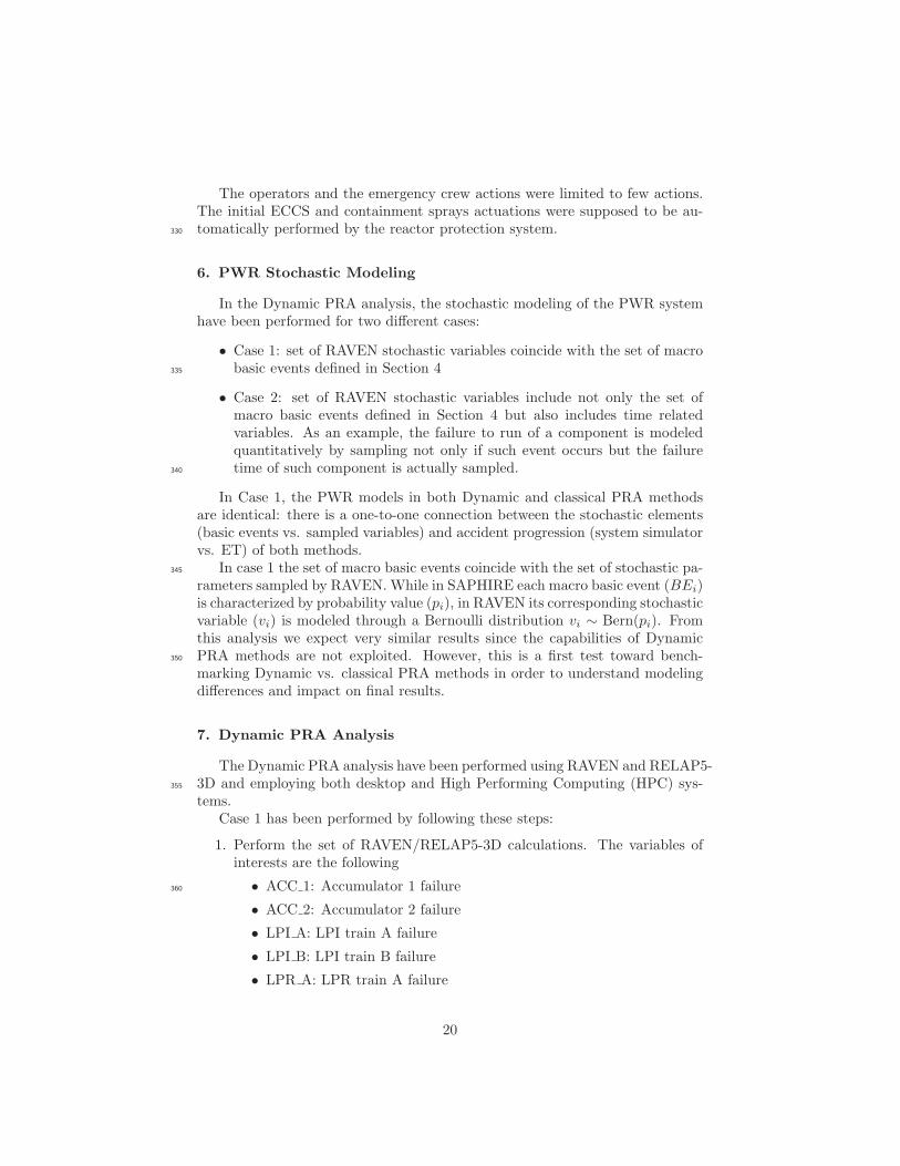
The operators and the emergency crew actions were limited to few actions.The initial ECCS and containment sprays actuations were supposed to be au-tomatically performed by the reactor protection system.330
6. PWR Stochastic Modeling
In the Dynamic PRA analysis, the stochastic modeling of the PWR systemhave been performed for two different cases:
• Case 1: set of RAVEN stochastic variables coincide with the set of macrobasic events defined in Section 4335
• Case 2: set of RAVEN stochastic variables include not only the set ofmacro basic events defined in Section 4 but also includes time relatedvariables. As an example, the failure to run of a component is modeledquantitatively by sampling not only if such event occurs but the failuretime of such component is actually sampled.340
In Case 1, the PWR models in both Dynamic and classical PRA methodsare identical: there is a one-to-one connection between the stochastic elements(basic events vs. sampled variables) and accident progression (system simulatorvs. ET) of both methods.
In case 1 the set of macro basic events coincide with the set of stochastic pa-345
rameters sampled by RAVEN. While in SAPHIRE each macro basic event (BEi)is characterized by probability value (pi), in RAVEN its corresponding stochasticvariable (vi) is modeled through a Bernoulli distribution vi ∼ Bern(pi). Fromthis analysis we expect very similar results since the capabilities of DynamicPRA methods are not exploited. However, this is a first test toward bench-350
marking Dynamic vs. classical PRA methods in order to understand modelingdifferences and impact on final results.
7. Dynamic PRA Analysis
The Dynamic PRA analysis have been performed using RAVEN and RELAP5-3D and employing both desktop and High Performing Computing (HPC) sys-355
tems.Case 1 has been performed by following these steps:
1. Perform the set of RAVEN/RELAP5-3D calculations. The variables ofinterests are the following
• ACC 1: Accumulator 1 failure360
• ACC 2: Accumulator 2 failure
• LPI A: LPI train A failure
• LPI B: LPI train B failure
• LPR A: LPR train A failure
20
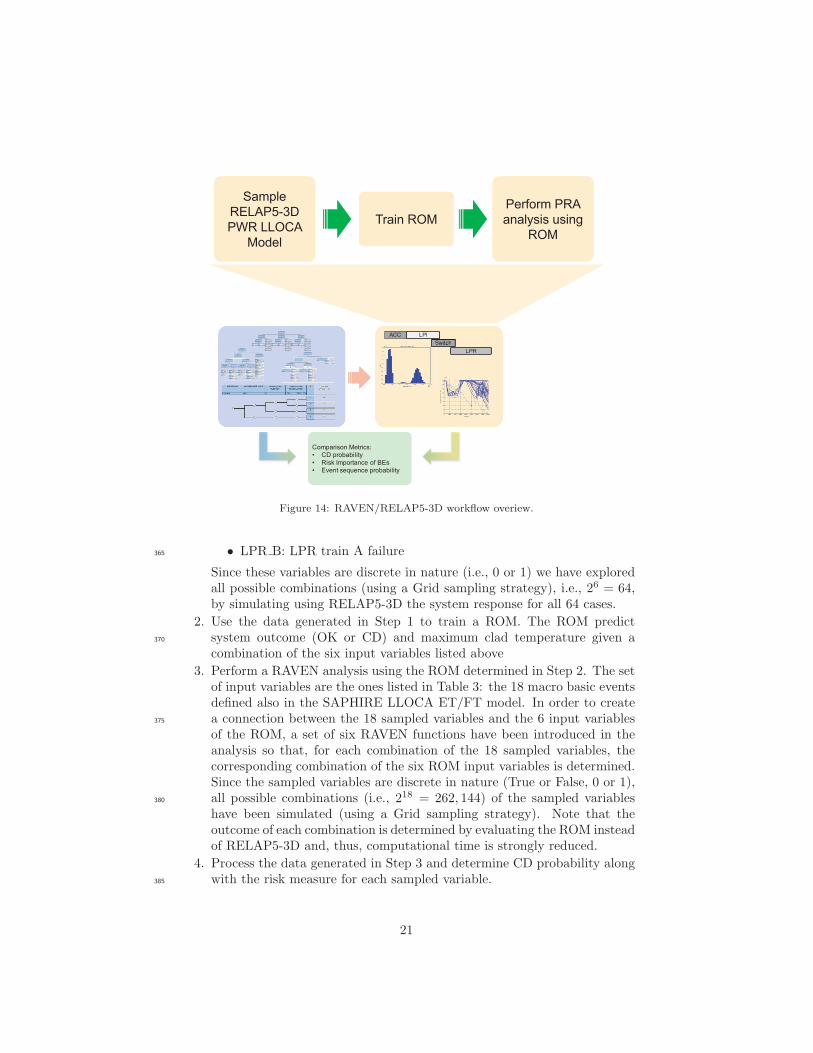
Figure 14: RAVEN/RELAP5-3D workflow overiew.
• LPR B: LPR train A failure365
Since these variables are discrete in nature (i.e., 0 or 1) we have exploredall possible combinations (using a Grid sampling strategy), i.e., 26 = 64,by simulating using RELAP5-3D the system response for all 64 cases.
2. Use the data generated in Step 1 to train a ROM. The ROM predictsystem outcome (OK or CD) and maximum clad temperature given a370
combination of the six input variables listed above
3. Perform a RAVEN analysis using the ROM determined in Step 2. The setof input variables are the ones listed in Table 3: the 18 macro basic eventsdefined also in the SAPHIRE LLOCA ET/FT model. In order to createa connection between the 18 sampled variables and the 6 input variables375
of the ROM, a set of six RAVEN functions have been introduced in theanalysis so that, for each combination of the 18 sampled variables, thecorresponding combination of the six ROM input variables is determined.Since the sampled variables are discrete in nature (True or False, 0 or 1),all possible combinations (i.e., 218 = 262, 144) of the sampled variables380
have been simulated (using a Grid sampling strategy). Note that theoutcome of each combination is determined by evaluating the ROM insteadof RELAP5-3D and, thus, computational time is strongly reduced.
4. Process the data generated in Step 3 and determine CD probability alongwith the risk measure for each sampled variable.385
21
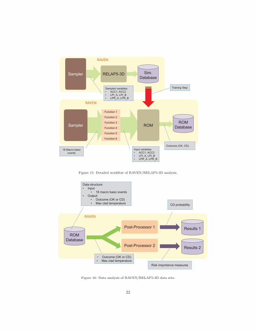
Figure 15: Detailed workflow of RAVEN/RELAP5-3D analysis.
Figure 16: Data analysis of RAVEN/RELAP5-3D data sets.
22
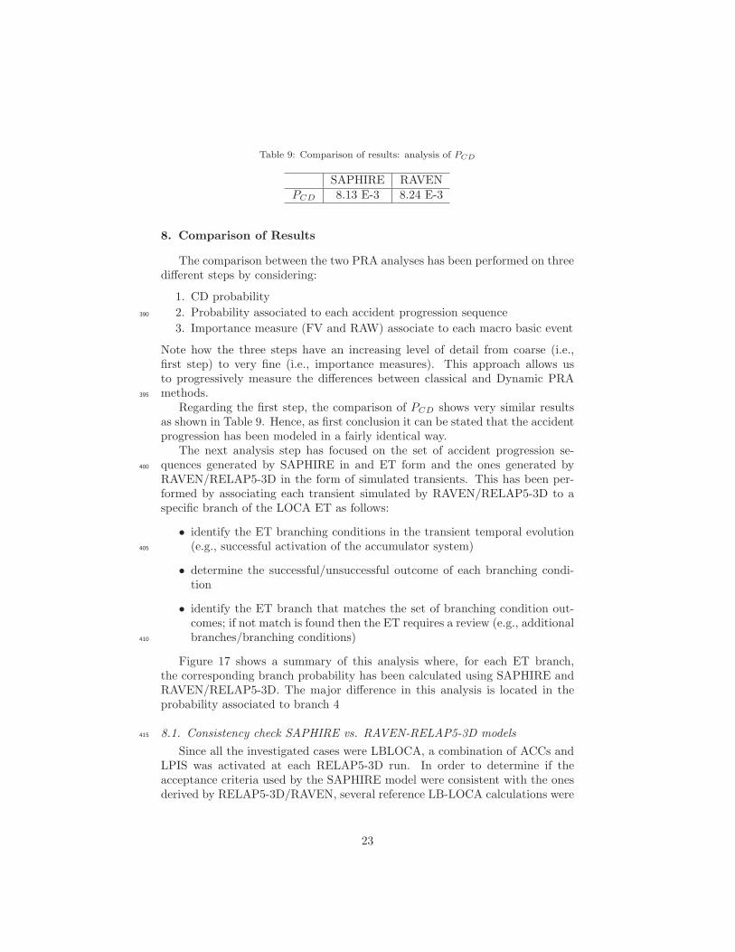
Table 9: Comparison of results: analysis of PCD
SAPHIRE RAVENPCD 8.13 E-3 8.24 E-3
8. Comparison of Results
The comparison between the two PRA analyses has been performed on threedifferent steps by considering:
1. CD probability
2. Probability associated to each accident progression sequence390
3. Importance measure (FV and RAW) associate to each macro basic event
Note how the three steps have an increasing level of detail from coarse (i.e.,first step) to very fine (i.e., importance measures). This approach allows usto progressively measure the differences between classical and Dynamic PRAmethods.395
Regarding the first step, the comparison of PCD shows very similar resultsas shown in Table 9. Hence, as first conclusion it can be stated that the accidentprogression has been modeled in a fairly identical way.
The next analysis step has focused on the set of accident progression se-quences generated by SAPHIRE in and ET form and the ones generated by400
RAVEN/RELAP5-3D in the form of simulated transients. This has been per-formed by associating each transient simulated by RAVEN/RELAP5-3D to aspecific branch of the LOCA ET as follows:
• identify the ET branching conditions in the transient temporal evolution(e.g., successful activation of the accumulator system)405
• determine the successful/unsuccessful outcome of each branching condi-tion
• identify the ET branch that matches the set of branching condition out-comes; if not match is found then the ET requires a review (e.g., additionalbranches/branching conditions)410
Figure 17 shows a summary of this analysis where, for each ET branch,the corresponding branch probability has been calculated using SAPHIRE andRAVEN/RELAP5-3D. The major difference in this analysis is located in theprobability associated to branch 4
8.1. Consistency check SAPHIRE vs. RAVEN-RELAP5-3D models415
Since all the investigated cases were LBLOCA, a combination of ACCs andLPIS was activated at each RELAP5-3D run. In order to determine if theacceptance criteria used by the SAPHIRE model were consistent with the onesderived by RELAP5-3D/RAVEN, several reference LB-LOCA calculations were
23
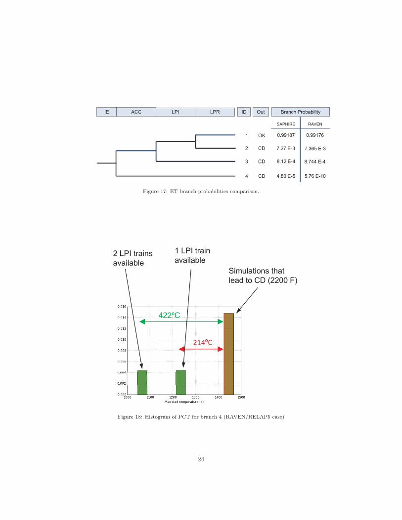
Figure 17: ET branch probabilities comparison.
Figure 18: Histogram of PCT for branch 4 (RAVEN/RELAP5 case)
24
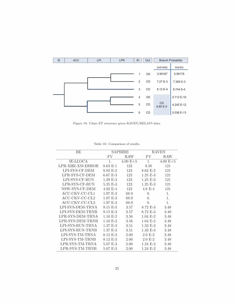
Figure 19: Udate ET structure given RAVEN/RELAP5 data.
Table 10: Comparison of results.
BE SAPHIRE RAVENFV RAW FV RAW
IE-LLOCA 1. 4.00 E+5 1. 4.00 E+5LPR-XHE-XM-ERROR 8.63 E-1 123 8.50 121
LPI-SYS-CF-DEM 8.82 E-2 123 8.62 E-2 121LPR-SYS-CF-DEM 6.67 E-3 123 1.25 E-3 121LPI-SYS-CF-RUN 1.29 E-3 123 1.25 E-3 121LPR-SYS-CF-RUN 5.25 E-3 123 1.25 E-3 121NSW-SYS-CF-DEM 4.92 E-4 123 4.8 E-4 121ACC-CKV-CC-CL1 1.97 E-3 68.9 0. 1.ACC-CKV-CC-CL2 1.97 E-3 68.9 0. 1.ACC-CKV-CC-CL3 1.97 E-3 68.9 0. 1.
LPI-SYS-DEM-TRNA 9.15 E-3 3.57 8.72 E-3 3.48LPI-SYS-DEM-TRNB 9.15 E-3 3.57 8.72 E-3 3.48LPR-SYS-DEM-TRNA 1.10 E-2 3.56 1.04 E-2 3.48LPR-SYS-DEM-TRNB 1.10 E-2 3.56 1.04 E-2 3.48LPI-SYS-RUN-TRNA 1.37 E-3 3.51 1.33 E-3 3.48LPI-SYS-RUN-TRNB 1.37 E-3 3.51 1.33 E-3 3.48LPI-SYS-TM-TRNA 8.12 E-3 2.00 2.0 E-2 3.48LPI-SYS-TM-TRNB 8.12 E-3 2.00 2.0 E-2 3.48LPR-SYS-TM-TRNA 5.07 E-3 2.00 1.24 E-2 3.48LPR-SYS-TM-TRNB 5.07 E-3 2.00 1.24 E-2 3.48
25
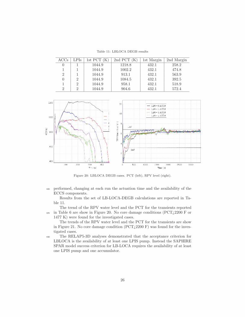
Table 11: LBLOCA DEGB results
ACCs LPIs 1st PCT (K) 2nd PCT (K) 1st Margin 2nd Margin0 1 1044.9 1218.8 432.1 258.21 1 1044.9 1002.2 432.1 474.82 1 1044.9 913.1 432.1 563.90 2 1044.9 1084.5 432.1 392.51 2 1044.9 958.1 432.1 518.92 2 1044.9 904.6 432.1 572.4
Figure 20: LBLOCA DEGB cases. PCT (left), RPV level (right).
performed, changing at each run the actuation time and the availability of the420
ECCS components.Results from the set of LB-LOCA-DEGB calculations are reported in Ta-
ble 11.The trend of the RPV water level and the PCT for the transients reported
in Table 6 are show in Figure 20. No core damage conditions (PCT¿2200 F or425
1477 K) were found for the investigated cases.The trends of the RPV water level and the PCT for the transients are show
in Figure 21. No core damage condition (PCT¿2200 F) was found for the inves-tigated cases.
The RELAP5-3D analyses demonstrated that the acceptance criterion for430
LBLOCA is the availability of at least one LPIS pump. Instead the SAPHIRESPAR model success criterion for LB-LOCA requires the availability of at leastone LPIS pump and one accumulator.
26
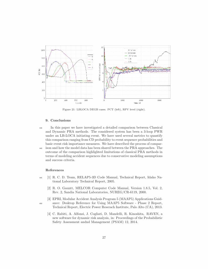
Figure 21: LBLOCA DEGB cases. PCT (left), RPV level (right).
9. Conclusions
In this paper we have investigated a detailed comparison between Classical435
and Dynamic PRA methods. The considered system has been a 3-loop PWRunder an LB-LOCA initiating event. We have used several metrics to quantifythis comparison ranging from CD probability to event sequence probabilities andbasic event risk importance measures. We have described the process of compar-ison and how the model data has been shared between the PRA approaches. The440
outcome of the comparison highlighted limitations of classical PRA methods interms of modeling accident sequences due to conservative modeling assumptionsand success criteria.
References
[1] R. C. D. Team, RELAP5-3D Code Manual, Technical Report, Idaho Na-445
tional Laboratory Technical Report, 2005.
[2] R. O. Gauntt, MELCOR Computer Code Manual, Version 1.8.5, Vol. 2,Rev. 2, Sandia National Laboratories, NUREG/CR-6119, 2000.
[3] EPRI, Modular Accident Analysis Program 5 (MAAP5) Applications Guid-ance: Desktop Reference for Using MAAP5 Software - Phase 2 Report,450
Technical Report, Electric Power Reserach Institute, Palo Alto (CA), 2013.
[4] C. Rabiti, A. Alfonsi, J. Cogliati, D. Mandelli, R. Kinoshita, RAVEN, anew software for dynamic risk analysis, in: Proceedings of the ProbabilisticSafety Assessment andnd Management (PSAM) 12, 2014.
27
[5] B. Rutt, U. Catalyurek, A. Hakobyan, K. Metzroth, T. Aldemir, R. Den-455
ning, S. Dunagan, D. Kunsman, Distributed dynamic event tree generationfor reliability and risk assessment, in: 2006 IEEE Challenges of Large Ap-plications in Distributed Environments, 2006, pp. 61–70.
[6] E. Hofer, M. Kloos, B. Krzykacz-Hausmann, J. Peschke, M. Woltereck,An approximate epistemic uncertainty analysis approach in the presence460
of epistemic and aleatory uncertainties, Reliability Engineering & SystemSafety 77 (2002) 229–238.
[7] K. S. Hsueh, A. Mosleh, The development and application of the acci-dent dynamic simulator for dynamic probabilistic risk assessment of nuclearpower plants, Reliability Engineering & System Safety 52 (1996) 297–314.465
[8] J. Devooght, C. Smidts, Probabilistic dynamics as a tool for dynamic PSA,Reliability Engineering & System Safety 52 (1996) 185 – 196.
[9] D. Mandelli, Z. Ma, C. Parisi, D. Maljovec, A. Alfonsi, C. Smith, Measuringrisk-importance in a simulation-based pra framework - part i: Mathemati-cal framework, Draft for Reliability Engineering & System Safety (2017).470
[10] C. Smith, J. Knudsen, D. ONeal, T. Peterson, K. Vedros, SAPHIRE 8 NewFeatures and Capabilities, Technical Report, Idaho National LaboratoryTechnical Report: INL/EXT-08-14841, 2008.
[11] E. P. R. Institute, Computer Aided Fault Tree Analysis System (CAFTA),Version 6.0b, Technical Report, Electric Power Research Institute, 2014.475
28