Risk Factors that Matter: Textual Analysis of Risk

Disclosures for the Cross-Section of Returns

Alejandro Lopez-Lira∗

The Wharton School

University of Pennsylvania

November 2018

Abstract

I introduce risk factors that not only explain the cross-section of returns, but also

unambiguously represent economic risk for the firms, are interpretable, and come di-

rectly from the companies. I exploit machine learning and natural language processing

techniques to identify from the 10-K annual reports the types of risks that firms face,

and to quantify how much each firm is exposed to each type of risk. I employ the

exposure of companies to each type of risk to construct portfolios exposed to specific

risks and construct a factor model with these portfolios. The model is not rejected by

the set of 49 Industry Portfolios using the GRS test, which is not the case for the Five

Factor Model of Fama and French (2015).

Keywords Cross-Section of Returns, Factor Models, Machine Learning, Big Data, LDA, Text

Analysis, NLP

∗I am grateful and acknowledge the financial support provided by the Mack Institute for InnovationManagement and the the Rodney L. White Center for Financial Research. I am grateful to Joao Gomes, AmirYaron, Jules van Binsbergen, Nick Roussanov, Winston Dou and Alexandr Belyakov for helpful discussionsand feedback. Please email me for the latest version: joselop@wharton.upenn.edu

1

1 Introduction

The goal of most of the empirical cross-sectional asset pricing literature is to explain why different

assets earn different returns, usually by specifying a linear factor model for excess returns:

rei,t+1 = αi,t + β′i,tft+1 + εi,t+1, (1)

with the important economic restriction1 that αi,t = 0. There is no consensus on how to choose the

factors, and researchers generally use one of three different approaches: empirical factors models

explicitly designed to overcome anomalies (portfolios of returns that are known to generate α),

factors constructed from economic theory and statistical factor models.

However, there have been major recent concerns about these approaches ,2 the main ones being

data mining, overfitting and p-hacking (that is, finding spurious correlations by repeatedly testing

variations of the data); the lack of theories for factors or characteristics designed to address anoma-

lies in the cross-section of returns;3 and concerns about the absence of economic interpretability

regarding purely statistical factors.4 I propose a new way of modelling the cross-section of returns

that avoids the usual concerns about factor models: I use machine learning techniques to extract

from the 10-K Annual Reports all of the risks that companies disclose, and use these risks to

construct a factor model with economically relevant risk factors.

Importantly, the machine learning approach that I use differs significantly from statistical factor

models. A typical statistical factor model uses realized returns to find factors that best fit the

cross-section. In my approach, I do not use information from the returns at all; I only use the

information that companies disclose in their annual reports. Hence, the factors that I identify have

a clear economic meaning and are fully and easily interpretable, rather than just being a linear

combination of returns.

1. Additionaly we require Et[εi,t] = Et[ei,t+1ft+1] = 0 and Et[ft+1] = λt.2. See Cochrane (2011), Harvey, Liu, and Zhu (2016), McLean and Pontiff (2016), and Hou, Xue, and

Zhang (2017)3. Fama and French (1993): ”the choice of factors, especially the size and book-to-market factors, is

motivated by empirical experience. Without a theory that specifies the exact form of the state variables orcommon factors in returns, the choice of any particular version of the factors is somewhat arbitrary”. Seealso Kelly, Pruitt, and Su (2018)

4. See Kozak, Nagel, and Santosh (2018)

2

I use the risks revealed by the companies to solve the common concerns about factor models

in the following way: First, to the best of my knowledge, this is the only paper to use the 10-K

textual data to construct a factor model,5 so the concerns about data mining or p-hacking should

be minimal. Second, instead of defining some risk factors or characteristics that seem subjectively

important, I take them directly from the firms, since they are the ones that best understand the

risks they face. Finally, the factors unambiguously represent economic risk faced by the companies.

To accomplish this, I characterize the types of risks that public companies consider the most

relevant and choose to disclose on their annual reports and quantify how much each company is

exposed to each type of risk. Equipped with the per firm proportion of the exposure to the disclosed

risks, I sort firms to get portfolios exposed to each specific risk, and form a factor model using the

risks considered important by each of the firms. I test the capacity of these factors to price the

cross-section of returns using the set of 49 industry portfolios.6

Although the main contribution is using machine learning techniques to discover interpretable

and economically relevant risk factors, the model has an statistical fit significantly better than the

Five-Factor Model of Fama and French (2015) in the test of the 49 industry portfolios. Crucially, it

explains the cross-sectional variation of returns: the GRS statistic7 that measures whether αit 6= 0

is .82, (compare to a GRS statistic of 1.55 for the Fama and French (2015) Model) and implies a

p-value of 68 %, that is, we can very comfortably reject the null hypothesis that αit 6= 0, so there

is no evidence of misspricing (for comparison, the p-value for the Fama and French (2015) Model

is 4.4 %, that is, we cannot reject the null hypothesis that αit 6= 0). In short, the GRS test says

that my model is a complete descriptions of expected returns for this set of portfolios.89

I extract the risks that companies disclose from the 10-K Annual reports using Latent Dirichlet

Allocation (LDA),10 a technique developed in the machine learning literature. LDA is a topic

modelling technique that summarizes the risks that firms are concerned about, and how much time

5. Note, however, that Israelsen (2014) was the first to apply LDA to construct portfolios, but uses themto perform factor analysis of the Fama-French factors

6. I choose these portfolios as a test set following the critique of Lewellen, Nagel, and Shanken (2010).7. Gibbons, Ross, and Shanken (1989)8. See the Appendix for other test sets9. Additionaly, it succeeds in explaining a large fraction of the time series variation of the cross-section of

returns (measured by an average R2 of 63 %, comparable to the 68% average R2 obtained with the Famaand French (2015) Model).

10. Blei, Ng, and Jordan (2003)

3

each company spends discussing each risk.11 With the additional assumption that if a company

spends a longer time discussing a specific risk, they are more exposed to that risk,12 we can quantify

how much each firm is exposed to each type of risk.

Ex-ante, the risks reported by the companies could be either idiosyncratic or systematic. I

select the systematic risks by choosing the portfolios with the highest Sharpe ratio13 and use these

portfolios to form a factor model. Note that no information about the 49 industry portfolios is

used to select the portfolios that are going to form the factor model, so I avoid both p-hacking and

data mining, in this sense, the test is actually an out-of-sample test. While choosing factors via the

individual Sharpe ratio provides a great statistical fit, it is not the only criteria that can be used

to select a the most important portfolios, see the Appendix for details.

The model has desirable properties over other models that also succeed in fitting the cross-

section of stock returns. A salient branch of the literature is concentrated on explaining the cross-

section of returns using statistical factors,14 and while they provide an outstanding statistical fit,

it is hard to understand the economics of these factors and whether they represent risk or are

generated by behavioral patterns (Kozak, Nagel, and Santosh (2018)), whereas by design, the

factors constructed from the firms’ risk disclosures represent economic risk.

Another historically important branch of the literature explains anomalies (portfolios with

α 6= 0) by iteratively adding (some of) the existing anomalies as risk factors.15 However adding

anomalies as risk factors naturally generates too many factors, a ”factor zoo” (Cochrane (2011)),

and disentangling the true risk factors from the anomalies is a complicated endeavor.16 To com-

plicate things further, there are important concerns as to which of these anomalies are actually

significant out-of-sample (Harvey, Liu, and Zhu (2016), McLean and Pontiff (2016)), so adding

them as risk factors is at best, risky. Since by design, all of the factors in the paper, represent risk,

it suffices to identify which of these factors are priced to get a set of risk factors that explains the

11. See Section 4 for a detailed explanation12. Gaulin (2017) and Campbell et al. (2014) find empirical evidence justifying this assumption: ”the type

of risk the firm faces determines whether it devotes a greater portion of its disclosures towards describingthat risk type”. See Section 3 for an extended discussion.

13. Sharpe (1966)14. See Kelly, Pruitt, and Su (2018), Kozak, Nagel, and Santosh (2018) and Section 2 Related Literature15. See for example Fama and French (1992), Fama and French (1993), Fama and French (2015), Hou,

Xue, and Zhang (2015), Stambaugh and Yuan (2017) among many, many others16. Feng, Giglio, and Xiu (2017) however, provide some hope to succeed.

4

cross-section.

Moreover, we know from Merton (1973) that the risk premia of every asset depends on the

covariances of the firms’ cash-flows with the market wealth and other state variables that affect the

stochastic discount factor (SDF). Any characteristic of the firms that makes their dividends covary

with either wealth or state variables would affect returns. Asking researchers to identify all of these

variables seems like an unworkable task. Firms, however, have a better understanding of the risk

they are facing. So instead of identifying all of the relevant characteristics, we can directly identify

all of the risks perceived by the firms by recovering them from all of the firms’ risk disclosures.

The paper continues as follows: Section 2 provides a (brief) literature review; Section 3 describes

the data sets and addresses concerns about the reliability of the annual reports; Section 4 describes

extensively the process to recover the types of risks from the annual reports; Section 5 describes the

characteristics of these risks; Section 6 describes the risk factors and tests; and Section 7 concludes.

The techniques used to extract the risks are fairly new to the finance field, so I encourage the reader

to read Section 4 before Section 5 or Section 6.

2 Related Literature

My paper makes contributions in two different branches of literature: machine learning and big

data methods in finance, and cross-sectional asset pricing.

There is a recent tradition of employing text analysis to study a variety of finance research

questions (see Loughran and McDonald (2016) for a systematic review). There are some papers

that employ text analysis to study a specific risk that the researchers have in mind (e.g. Hassan,

Hollander, van Lent and Tahoun (2017) for political risk; Hanley and Hoberg (2017) for financial

risk). I instead, do not specify any risk ex-ante and instead let them arise naturally from the data

using unsupervised learning. One important predecessor of my paper is Israelsen (2014), who uses

LDA to perform style analysis between disclosed risks and the Fama-French factors. I build on his

paper by using the risks disclosed by the firms to form a factor model that explains the cross-section

of returns.

My paper is of course related to the large literature on cross-sectional stock returns (see, e.g.,

5

Cochrane (1991); Berk, Green, and Naik (1999); Gomes, Kogan, and Zhang (2003); Nagel (2005);

Zhang (2005); Livdan, Sapriza, and Zhang (2009);Eisfeldt and Papanikolaou (2013); Kogan and

Papanikolaou (2014)). See Harvey, Liu, and Zhu (2016) for a recent systematic survey. However,

to the best of my knowledge, this is the first paper to construct a successful factor model using all

of the risks disclosed by the firms

3 Data

I use three sources of data: the 10-Ks Annual Reports, Compustat, and CRSP.

3.1 10-K Annual Reports

Firms disclose in their annual reports which types of risk they are facing. There can be some

concerns about how true and informative these disclosures are, however, there exist ample evidence

that risk disclosure are, indeed, useful and informative. First, firms are legally required to to discuss

”the most significant factors that make the company speculative or risky” (Regulation S–K, Item

305(c), SEC 2005) in a specific section of the 10-K annual reports (Section 1A) and could face legal

action if they fail to obey the regulation. Additionally, Campbell et al. (2014) find that ”firms

facing greater risk disclose more risk factors”, ”the type of risk the firm faces determines whether

it devotes a greater portion of its disclosures towards describing that risk type”, ”managers provide

risk factor disclosures that meaningfully reflect the risks they face” and ”the disclosures appear to

be (...) specific and useful to investors”.

I extract the textual risk factors in Section 1A (mandatory since 2005) of each 10-K Annual

Report. I collect the 10-Ks from 2005 to 2018 from the EDGAR database on the SEC’s website.

The 10-Ks come in many different file formats (.txt., .xml, and .html) and have different formatting,

so it is quite challenging to automatically extract the Section 1A-Risk Factors, from the 10-K forms.

I first detect and remove the markup language and then use regular expressions with predefined

heuristic rules to extract these sections. I end up with a data set consisting of 79304 documents.

An excerpt of the 10-K annual report of Apple Inc. for the year 2010 illustrates the kind of

disclosures that firms make. I incorporate suggested labels regarding the type of risk, as well as

6

highlight possible key words in red. Note that both labels and key words are just for illustrative

purposes, and there is no need to manually label the risks in the paper or define the keywords,

since the risk factors will arise naturally using the LDA algorithm.

• Currency Risk: ”Demand (...) could differ (...) since the Company generally raises prices on

goods and services sold outside the U.S. to offset the effect of the strengthening of the U.S.

dollar change”.

• Supplier Risk: ”The Company uses some custom components that are not common to the

rest of the personal computer, mobile communication and consumer electronics industries.”

• Competition Risk: ”Due to the highly volatile and competitive nature of the personal com-

puter, mobile communication and consumer electronics industries, the Company must con-

tinually introduce new products”

3.2 CRSP and Compustat

I follow the usual conventions regarding CRSP and Compustat data. I focus on monthly returns

since the disclosures are done annually. For the accounting and return data, I use the the merged

CRSP/Compustat database. I use annual firm-level balance sheet data from Compustat due to

concerns about seasonality and precision; and monthly returns from CRSP. I use data from the

same period as the one where 10-Ks are available: 2005-2018, although not all variables are available

for every period. I exclude from the main analysis firms in industries with SIC codes corresponding

to financial (SIC in [6000, 7000]).

The Five Factors of Fama and French (2015), the momentum factor, and the one-month

Treasury-bill rate come from the French data library on Ken French’s website. The Stambaugh

and Yuan (2017) factors come from their website. The q-factors of Hou, Xue, and Zhang (2015)

come from their website.

7

4 Text Processing

Figure 1: Steps for topic modelling

4.1 Bag of Words and Document Term Matrix

We need a way to represent text data for statistical purposes. The bag-of-words model achieves this

task. Bag of Words considers text as a list of distinct words in a document and a word count for

each word,17 which implies that each document is represented as a fixed-length vector with length

equal to the vocabulary size. Each dimension of this vector corresponds to the count or occurrence

of a word in a document. Traditionally, all words are lowercased to reduce the dimension in half.

It is called a “bag” of words, because any information about the order or structure of words in

the document is discarded. The model is only concerned with whether known words occur in the

document, not where in the document. Notice that since we only consider the count, the order of

the words is lost. When we consider several documents at a time, we end up with a Document Term

Matrix (DTM), see Figure 2 for a simplified example. The DTM is typically very high dimensional

(> 10,000 columns), since we consider the space of all words used across all documents, it is also

very sparse, since typically documents do not use the whole English vocabulary. Because of the

huge dimension of the space, we need a dimentionality reduction technique, such as LDA.

Another subtle disadvantage is that it breaks multi-word concepts such as ”real state” into

”real” and ”state”, which have to be rejoined later, since counting those words separately will be

17. Manning, Raghavan, and Schutze (2008)

8

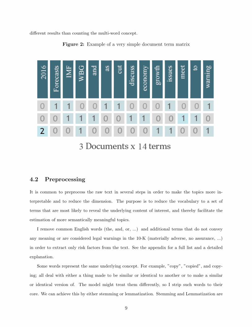
different results than counting the multi-word concept.

Figure 2: Example of a very simple document term matrix

4.2 Preprocessing

It is common to preprocess the raw text in several steps in order to make the topics more in-

terpretable and to reduce the dimension. The purpose is to reduce the vocabulary to a set of

terms that are most likely to reveal the underlying content of interest, and thereby facilitate the

estimation of more semantically meaningful topics.

I remove common English words (the, and, or, ...) and additional terms that do not convey

any meaning or are considered legal warnings in the 10-K (materially adverse, no assurance, ...)

in order to extract only risk factors from the text. See the appendix for a full list and a detailed

explanation.

Some words represent the same underlying concept. For example, ”copy”, ”copied”, and copy-

ing; all deal with either a thing made to be similar or identical to another or to make a similar

or identical version of. The model might treat them differently, so I strip such words to their

core. We can achieve this by either stemming or lemmatization. Stemming and Lemmatization are

9

fundamental text processing methods for text in the English language.

Stemming helps to create groups of words which have similar meanings and works based on a

set of rules, such as remove “ing” if words are ending with “ing”.18 Different types of stemmers

are available in standard text processing software such as NLTK (Loper and Bird (2002)), and

within the stemmers there are different versions such as PorterStemmer, LancasterStemmer and

SnowballStemmer. The disadvantages of stemming is that it cannot relate words which have

different forms based on grammatical constructs, for example: ”is”, ”am”, and ”be” come form

same root verb, ”be”, but stemming cannot prune them to their common form . Another example:

the word better should be resolved to good, but stemmers would fail to do that. With stemming,

there is lot of ambiguity which may cause several different concepts to appear related. Axes is both

a plural form of axe and axis. By chopping of the ”s”, there is no way to distinguish between the

two.

Lemmatization in linguistics is the process of grouping together the inflected forms of a word so

they can be analyzed as a single item, identified by the word’s lemma, or dictionary form(Manning,

Raghavan, and Schutze (2008)). In order to relate different inflectional forms to their common

base form, it uses a knowledge base called WordNet. With the use of this knowledge base, lemma-

tization can convert words which have a different form and cannot be solved by stemmers, for

example converting “are” to “be”. The disadvantages of lemmatization are that it is slower com-

pared to stemming, however, I use lemmatization to preserve meaning and make the topics more

understandable.

Phrase Modeling is another useful technique whose purpose is to (re)learn combinations of

tokens that together represent meaningful multi-word concepts. We can develop phrase models by

looking for words that co-occur (i.e., appear one after another) together much more frequently than

you would expect them to by random chance. The formula to determine whether two tokens A and

B constitute a phrase is:

count(A,B)−countmin

count(A)∗count(B) ∗N ≥ threshold , where:

• count(A) is the number of times token A appears in the corpus

18. Manning, Raghavan, and Schutze (2008)

10

• count(B) is the number of times token B appears in the corpus

• count(A,B) is the number of times the tokens A and B appear in the corpus in that order

• N is the total size of the corpus vocabulary

• countmin is a parameter to ensure that accepted phrases occur a minimum number of times

• threshold is a parameter to control how strong of a relationship between two tokens the

model requires before accepting them as a phrase

With phrase modeling, named entities will become phrases in the model (so new york would

become new york). We also would expect multi-word expressions that represent common concepts,

but are not named entities (such as real state) to also become phrases in the model.

4.3 Dictionary methods

The most common approach to text analysis in economics relies on dictionary methods, in which

the researcher defines a set of words of interest and then computes their counts or frequencies

across documents. However, this method has the disadvantage of subjectivity from the researcher

perspective since someone has to pick the words. Furthermore, it is very hard to get the full list of

words related to one concept and the dictionary methods assume the same importance or weight for

every word. Since the purpose of the paper is to extract the risks that managers consider important

with minimum researcher input, dictionary methods are unsatisfactory.

Furthermore, dictionary methods have other disadvantages, Hansen, McMahon, and Prat (2018)

say: ”For example, to measure economic activity, we might construct a word list which includes

‘growth’. But clearly other words are also used to discuss activity, and choosing these involves

numerous subjective judgments. More subtly, ‘growth’ is also used in other contexts, such as

in describing wage growth as a factor in inflationary pressures, and accounting for context with

dictionary methods is practically very difficult.”

For the purpose of studying the cross-section of returns, the problem is similar to picking

which characteristics are important for the returns. The dictionary methods would be equivalent

11

to manually picking which characteristics would enter a regression. The following algorithm, Topic

Modelling, is akin to automatic selection methods, such as LASSO (Tibshirani (1996)).

4.4 Topic Models

A topic model is a type of statistical model for discovering a set of topics that describe a collection

of documents based on the statistics of the words in each document, and the percentage that each

document spends in each topic. Since in this case, the documents are the risk disclosures from the

annual statements and they only concern risks, the topics discovered will correspond to different

types of risks.

Intuitively, given that a document is about a particular topic, one would expect particular

words to appear in the document more or less frequently. For example: ”internet” and ”users”

will appear more often in documents produced by firms in the technology sector; ”oil”, ”natural

gas” and ”drilling” will appear more frequently in documents produced by firms in the oil industry,

while ”company” and ”cash” would appear similarly in both.

A document typically concerns multiple topics, or in this case risks, in different proportions;

thus, in a company that is concerned with 20% about financial risks and 20% about internet

operations, the risk report would approximately have around 8 times more technology words than

financial words.

Because of the large number of firms in the stock market, the amount of time to read, categorize

and quantify the risks disclosed by every firm is simply beyond human capacity, but topic models

are capable of identifying these risks.

The most common topic model currently in use is the LDA model proposed by Blei, Ng, and

Jordan (2003). The model generates automatic summaries of topics in terms of a discrete proba-

bility distribution over words for each topic, and further infers per-document discrete distributions

over topics. The interaction between the observed documents and the hidden topic structure is

manifested in the probabilistic generative process associated with LDA.

12

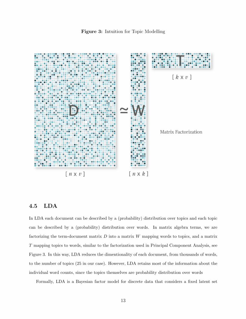
Figure 3: Intuition for Topic Modelling

4.5 LDA

In LDA each document can be described by a (probability) distribution over topics and each topic

can be described by a (probability) distribution over words. In matrix algebra terms, we are

factorizing the term-document matrix D into a matrix W mapping words to topics, and a matrix

T mapping topics to words, similar to the factorization used in Principal Component Analysis, see

Figure 3. In this way, LDA reduces the dimentionality of each document, from thousands of words,

to the number of topics (25 in our case). However, LDA retains most of the information about the

individual word counts, since the topics themselves are probability distribution over words

Formally, LDA is a Bayesian factor model for discrete data that considers a fixed latent set

13

of topics. Suppose there are D documents that comprise a corpus of texts with V unique terms.

The K topics (in this case, risk types), are probability vectors βk ∈ ∆V−1 over the V unique terms

in the data, where ∆M refers to the M-dimensional simplex. By using probability distributions,

we allow the same term to appear in different topics with potentially different weights. We can

think of a topic as a weighted word vector that puts higher mass in words that all express the same

underlying theme.19

In LDA, each document is described by a distribution over topics it belongs, so each document

d has its own distribution over topics given by θd (in our case, how much each company discuss

each type of risk). Within a given document, each word is influenced by two factors, the topics

proportions for that document, θdk, and the probability measure over the words within the topics.

Formally, The probability that a word in document d is equal to the nth term is pdnθkd .

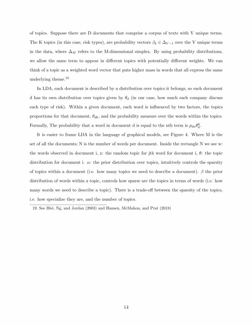
It is easier to frame LDA in the language of graphical models, see Figure 4. Where M is the

set of all the documents; N is the number of words per document. Inside the rectangle N we see w:

the words observed in document i, z: the random topic for jth word for document i, θ: the topic

distribution for document i. α: the prior distribution over topics, intuitively controls the sparsity

of topics within a document (i.e. how many topics we need to describe a document). β the prior

distribution of words within a topic, controls how sparse are the topics in terms of words (i.e. how

many words we need to describe a topic). There is a trade-off between the sparsity of the topics,

i.e. how specialize they are, and the number of topics.

19. See Blei, Ng, and Jordan (2003) and Hansen, McMahon, and Prat (2018)

14

Figure 4: LDA Graphical Model

4.5.1 Number of topics

The number of topics is a hyperparameter in LDA. Ideally, there should be enough topics to be able

to distinguish between themes in the text, but not so many that they lose their interpretability. In

this case 25 topics accomplish these task, and is consistent with the numbers used in the literature

(Israelsen (2014), Bao and Datta (2014)).

There are technical measures such as perplexity or predictive likelihood to help determine the

optimal number of topics from a statistical point of view. These measures are rarely use however,

because these metrics are not correlated with human interpretability of the model and prescribe a

very high number of topics, whereas for topic models, we care about getting interpretable topics

(which correspond to the type of risks).

In the case of risk disclosures, a low number (< 20) gets few common risks that all firms in

all industries face, and a big number (> 50) starts capturing very specific industry risks. Another

issue is that with a big number of topics, very few firms will have significant exposure to each risk,

and hence portfolios exposed to some risks will be poorly diversified. I set the number of topics

equal to 25 after experimenting with different values.

15

A natural challenge is then to further reduce the extracted risks into a lower number of portfolios

for the cross-section. I use the number of firms threshold, cross-validation, and with LASSO to

address this challenge. See the section Portfolios for more detail.

4.5.2 Estimation

The estimation of the posterior parameters is done using the open-source software GensimRehurek

and Sojka (2010) which runs on Python. Gensim uses an online Variational Bayes algorithm.

Because of the huge size of the collection of annual reports, the use of online algorithms allows

us to not load every document into the RAM memory and hence we can estimate the model in a

normal laptop. See the Appendix and Hoffman, Bach, and Blei (2010) for details.

5 Risk Topics and Risk Factors

We can get a general picture of the risks that firms are facing from Figure 5, where I present the 25

risk topics extracted from the 10-K annual report, recall from Section 4 that a topic is a probability

distribution over words. I discuss here only the risks that I will use for the factor model, the ones

with the highest Sharpe ratio, and discuss the rest in the Appendix.

16

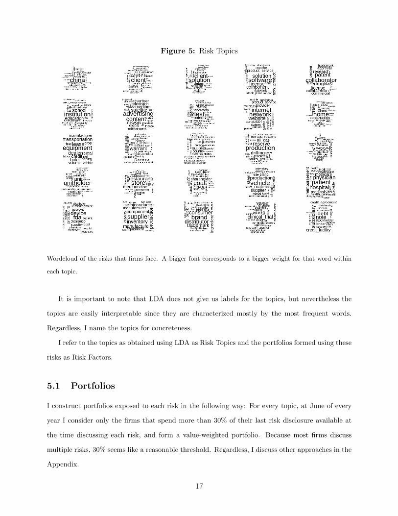
Figure 5: Risk Topics

Wordcloud of the risks that firms face. A bigger font corresponds to a bigger weight for that word within

each topic.

It is important to note that LDA does not give us labels for the topics, but nevertheless the

topics are easily interpretable since they are characterized mostly by the most frequent words.

Regardless, I name the topics for concreteness.

I refer to the topics as obtained using LDA as Risk Topics and the portfolios formed using these

risks as Risk Factors.

5.1 Portfolios

I construct portfolios exposed to each risk in the following way: For every topic, at June of every

year I consider only the firms that spend more than 30% of their last risk disclosure available at

the time discussing each risk, and form a value-weighted portfolio. Because most firms discuss

multiple risks, 30% seems like a reasonable threshold. Regardless, I discuss other approaches in the

Appendix.

17

To construct excess return portfolios, I substract the risk-free rate. Conceptually, because the

firms that spend 0% of their risk disclosure discussing a specific risk, must be spending that time

discussing other risks (I discard firms with no risk disclosures), if I substract portfolios composed

of the remaining firms, I am effectively mixing risks in an unknown proportion, which would result

in not understanding the risk the portfolio is representing, defeating the purpose of the exercise.

5.2 Consumer Demand Risk

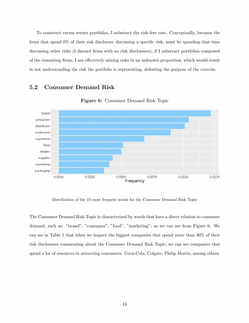
Figure 6: Consumer Demand Risk Topic

Distribution of the 10 most frequent words for the Consumer Demand Risk Topic

The Consumer Demand Risk Topic is characterized by words that have a direct relation to consumer

demand, such as: ”brand”, ”consumer”, ”food”, ”marketing”; as we can see from Figure 6. We

can see in Table 1 that when we inspect the biggest companies that spend more than 30% of their

risk disclosures commenting about the Consumer Demand Risk Topic, we can see companies that

spend a lot of resources in attracting consumers: Coca-Cola, Colgate, Philip Morris, among others.

18

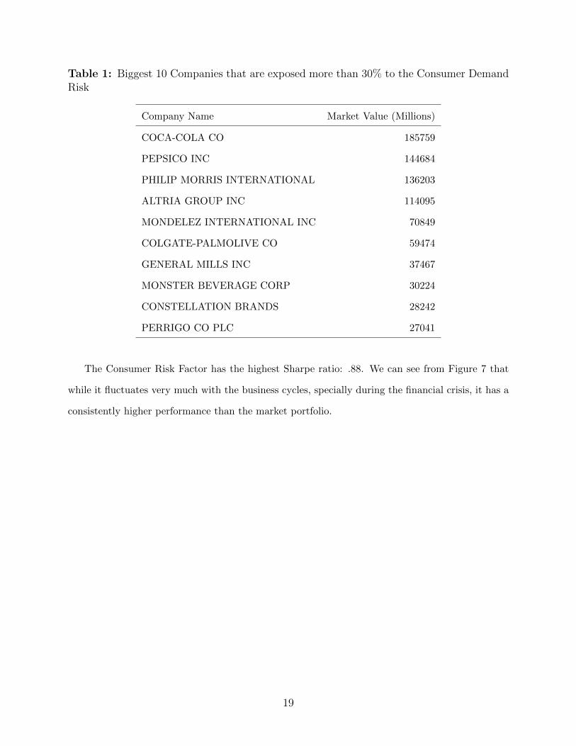
Table 1: Biggest 10 Companies that are exposed more than 30% to the Consumer DemandRisk

Company Name Market Value (Millions)

COCA-COLA CO 185759

PEPSICO INC 144684

PHILIP MORRIS INTERNATIONAL 136203

ALTRIA GROUP INC 114095

MONDELEZ INTERNATIONAL INC 70849

COLGATE-PALMOLIVE CO 59474

GENERAL MILLS INC 37467

MONSTER BEVERAGE CORP 30224

CONSTELLATION BRANDS 28242

PERRIGO CO PLC 27041

The Consumer Risk Factor has the highest Sharpe ratio: .88. We can see from Figure 7 that

while it fluctuates very much with the business cycles, specially during the financial crisis, it has a

consistently higher performance than the market portfolio.

19

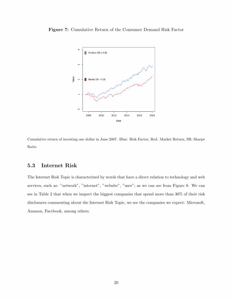
Figure 7: Cumulative Return of the Consumer Demand Risk Factor

Cumulative return of investing one dollar in June 2007. Blue: Risk Factor, Red: Market Return, SR: Sharpe

Ratio

5.3 Internet Risk

The Internet Risk Topic is characterized by words that have a direct relation to technology and web

services, such as: ”network”, ”internet”, ”website”, ”user”; as we can see from Figure 8. We can

see in Table 2 that when we inspect the biggest companies that spend more than 30% of their risk

disclosures commenting about the Internet Risk Topic, we see the companies we expect: Microsoft,

Amazon, Facebook, among others.

20

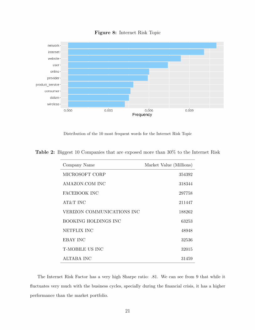
Figure 8: Internet Risk Topic

Distribution of the 10 most frequent words for the Internet Risk Topic

Table 2: Biggest 10 Companies that are exposed more than 30% to the Internet Risk

Company Name Market Value (Millions)

MICROSOFT CORP 354392

AMAZON.COM INC 318344

FACEBOOK INC 297758

AT&T INC 211447

VERIZON COMMUNICATIONS INC 188262

BOOKING HOLDINGS INC 63253

NETFLIX INC 48948

EBAY INC 32536

T-MOBILE US INC 32015

ALTABA INC 31459

The Internet Risk Factor has a very high Sharpe ratio: .81. We can see from 9 that while it

fluctuates very much with the business cycles, specially during the financial crisis, it has a higher

performance than the market portfolio.

21

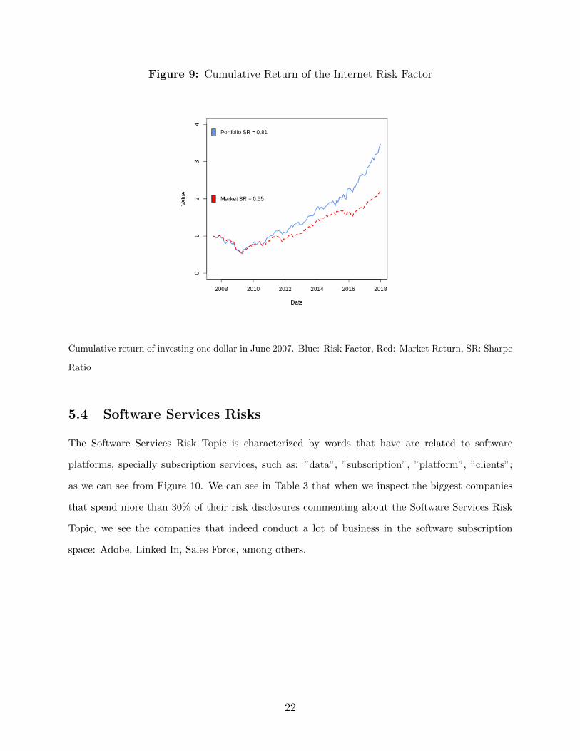
Figure 9: Cumulative Return of the Internet Risk Factor

Cumulative return of investing one dollar in June 2007. Blue: Risk Factor, Red: Market Return, SR: Sharpe

Ratio

5.4 Software Services Risks

The Software Services Risk Topic is characterized by words that have are related to software

platforms, specially subscription services, such as: ”data”, ”subscription”, ”platform”, ”clients”;

as we can see from Figure 10. We can see in Table 3 that when we inspect the biggest companies

that spend more than 30% of their risk disclosures commenting about the Software Services Risk

Topic, we see the companies that indeed conduct a lot of business in the software subscription

space: Adobe, Linked In, Sales Force, among others.

22

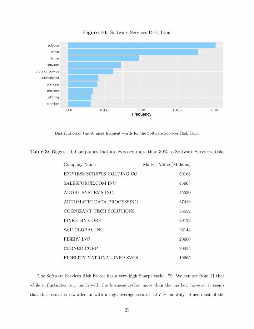
Figure 10: Software Services Risk Topic

Distribution of the 10 most frequent words for the Software Services Risk Topic

Table 3: Biggest 10 Companies that are exposed more than 30% to Software Services Risks

Company Name Market Value (Millions)

EXPRESS SCRIPTS HOLDING CO 59168

SALESFORCE.COM INC 45663

ADOBE SYSTEMS INC 45530

AUTOMATIC DATA PROCESSING 37419

COGNIZANT TECH SOLUTIONS 36552

LINKEDIN CORP 29722

S&P GLOBAL INC 26143

FISERV INC 20606

CERNER CORP 20455

FIDELITY NATIONAL INFO SVCS 19665

The Software Services Risk Factor has a very high Sharpe ratio: .79. We can see from 11 that

while it fluctuates very much with the business cycles, more than the market, however it seems

that this return is rewarded in with a high average return: 1.07 % monthly. Since most of the

23

companies in the portfolio are in the business to business industry it seems intuitive that it varies

much more than the market portfolio, since we know investment is very volatile.

Figure 11: Cumulative Return of the Software Services Risk Factor

Cumulative return of investing one dollar in June 2007. Blue: Risk Factor, Red: Market Return, SR: Sharpe

Ratio

5.5 Health and Innovation Risks

The Health and Innovation Risk Topic is characterized by words that have are related to medicine

and innovation, such as: ”medical device”, ”FDA”, ”procedure”, ”patients”; as we can see from

Figure 12. We can see in Table 4 that when we inspect the biggest companies that spend more

than 30% of their risk disclosures commenting about the Health Service Risk Topic, we see the

companies we expect: Microsoft, Amazon, Facebook, among others.

24

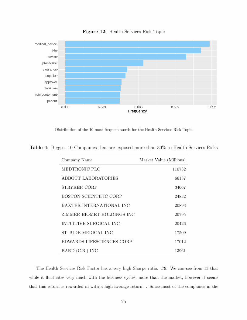
Figure 12: Health Services Risk Topic

Distribution of the 10 most frequent words for the Health Services Risk Topic

Table 4: Biggest 10 Companies that are exposed more than 30% to Health Services Risks

Company Name Market Value (Millions)

MEDTRONIC PLC 110732

ABBOTT LABORATORIES 66137

STRYKER CORP 34667

BOSTON SCIENTIFIC CORP 24832

BAXTER INTERNATIONAL INC 20893

ZIMMER BIOMET HOLDINGS INC 20795

INTUITIVE SURGICAL INC 20426

ST JUDE MEDICAL INC 17509

EDWARDS LIFESCIENCES CORP 17012

BARD (C.R.) INC 13961

The Health Services Risk Factor has a very high Sharpe ratio: .79. We can see from 13 that

while it fluctuates very much with the business cycles, more than the market, however it seems

that this return is rewarded in with a high average return: . Since most of the companies in the

25

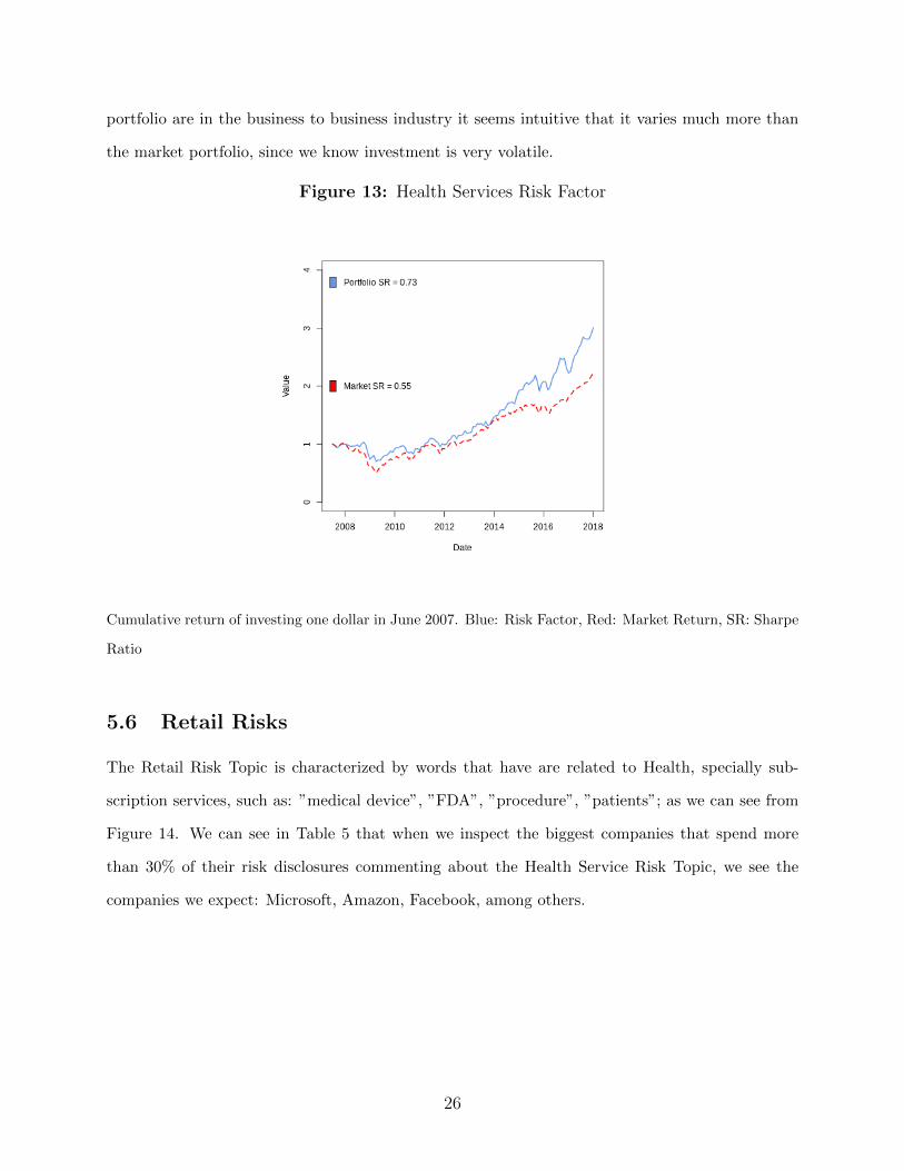
portfolio are in the business to business industry it seems intuitive that it varies much more than

the market portfolio, since we know investment is very volatile.

Figure 13: Health Services Risk Factor

Cumulative return of investing one dollar in June 2007. Blue: Risk Factor, Red: Market Return, SR: Sharpe

Ratio

5.6 Retail Risks

The Retail Risk Topic is characterized by words that have are related to Health, specially sub-

scription services, such as: ”medical device”, ”FDA”, ”procedure”, ”patients”; as we can see from

Figure 14. We can see in Table 5 that when we inspect the biggest companies that spend more

than 30% of their risk disclosures commenting about the Health Service Risk Topic, we see the

companies we expect: Microsoft, Amazon, Facebook, among others.

26

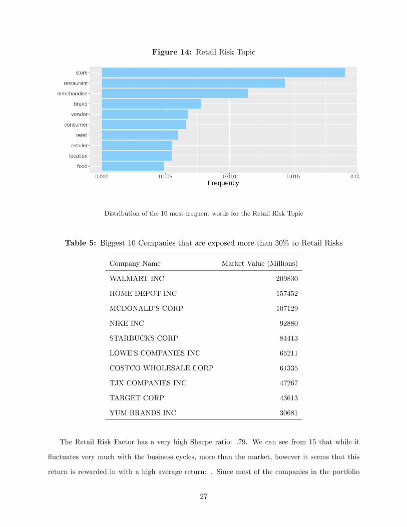
Figure 14: Retail Risk Topic

Distribution of the 10 most frequent words for the Retail Risk Topic

Table 5: Biggest 10 Companies that are exposed more than 30% to Retail Risks

Company Name Market Value (Millions)

WALMART INC 209830

HOME DEPOT INC 157452

MCDONALD’S CORP 107129

NIKE INC 92880

STARBUCKS CORP 84413

LOWE’S COMPANIES INC 65211

COSTCO WHOLESALE CORP 61335

TJX COMPANIES INC 47267

TARGET CORP 43613

YUM BRANDS INC 30681

The Retail Risk Factor has a very high Sharpe ratio: .79. We can see from 15 that while it

fluctuates very much with the business cycles, more than the market, however it seems that this

return is rewarded in with a high average return: . Since most of the companies in the portfolio

27

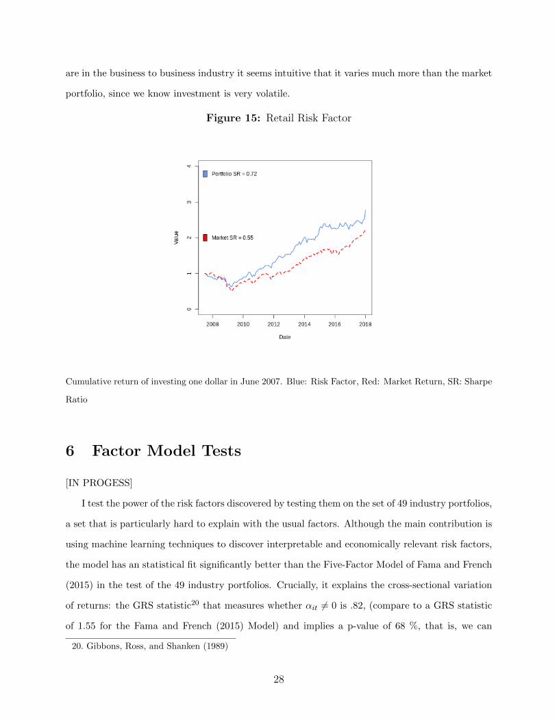
are in the business to business industry it seems intuitive that it varies much more than the market

portfolio, since we know investment is very volatile.

Figure 15: Retail Risk Factor

Cumulative return of investing one dollar in June 2007. Blue: Risk Factor, Red: Market Return, SR: Sharpe

Ratio

6 Factor Model Tests

[IN PROGESS]

I test the power of the risk factors discovered by testing them on the set of 49 industry portfolios,

a set that is particularly hard to explain with the usual factors. Although the main contribution is

using machine learning techniques to discover interpretable and economically relevant risk factors,

the model has an statistical fit significantly better than the Five-Factor Model of Fama and French

(2015) in the test of the 49 industry portfolios. Crucially, it explains the cross-sectional variation

of returns: the GRS statistic20 that measures whether αit 6= 0 is .82, (compare to a GRS statistic

of 1.55 for the Fama and French (2015) Model) and implies a p-value of 68 %, that is, we can

20. Gibbons, Ross, and Shanken (1989)

28

very comfortably reject the null hypothesis that αit 6= 0, so there is no evidence of misspricing

(for comparison, the p-value for the Fama and French (2015) Model is 4.4 %, that is, we cannot

reject the null hypothesis that αit 6= 0). In short, the GRS test says that my model is a complete

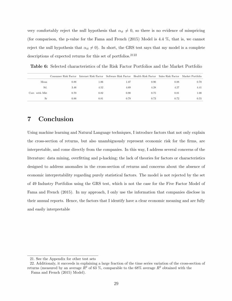
descriptions of expected returns for this set of portfolios.2122

Table 6: Selected characteristics of the Risk Factor Portfolios and the Market Portfolio

Consumer Risk Factor Internet Risk Factor Software Risk Factor Health Risk Factor Sales Risk Factor Market Portfolio

Mean 0.88 1.06 1.07 0.90 0.88 0.70

Sd. 3.46 4.52 4.69 4.28 4.27 4.41

Corr. with Mkt 0.70 0.82 0.90 0.75 0.81 1.00

Sr 0.88 0.81 0.79 0.73 0.72 0.55

7 Conclusion

Using machine learning and Natural Language techniques, I introduce factors that not only explain

the cross-section of returns, but also unambiguously represent economic risk for the firms, are

interpretable, and come directly from the companies. In this way, I address several concerns of the

literature: data mining, overfitting and p-hacking; the lack of theories for factors or characteristics

designed to address anomalies in the cross-section of returns and concerns about the absence of

economic interpretability regarding purely statistical factors. The model is not rejected by the set

of 49 Industry Portfolios using the GRS test, which is not the case for the Five Factor Model of

Fama and French (2015). In my approach, I only use the information that companies disclose in

their annual reports. Hence, the factors that I identify have a clear economic meaning and are fully

and easily interpretable

21. See the Appendix for other test sets22. Additionaly, it succeeds in explaining a large fraction of the time series variation of the cross-section of

returns (measured by an average R2 of 63 %, comparable to the 68% average R2 obtained with theFama and French (2015) Model).

29

References

Bao, Yang, and Anindya Datta. 2014. “Simultaneously Discovering and Quantifying Risk

Types from Textual Risk Disclosures.” Manage. Sci. (Institute for Operations Re-

search)(the Management Sciences (INFORMS), Linthicum, Maryland, USA) 60, no.

6 (June): 1371–1391. issn: 0025-1909. doi:10.1287/mnsc.2014.1930. https://doi.

org/10.1287/mnsc.2014.1930.

Berk, Jonathan B., Richard C. Green, and Vasant Naik. 1999. “Optimal Investment, Growth

Options, and Security Returns.” The Journal of Finance 54 (5): 1553–1607. issn: 1540-

6261. doi:10.1111/0022-1082.00161. http://dx.doi.org/10.1111/0022-1082.

00161.

Blei, David M., Andrew Y. Ng, and Michael I. Jordan. 2003. “Latent Dirichlet Allocation.”

J. Mach. Learn. Res. 3 (March): 993–1022. issn: 1532-4435. http://dl.acm.org/

citation.cfm?id=944919.944937.

Campbell, John L., Hsinchun Chen, Dan S Dhaliwal, Hsin min Lu, and Logan B. Steele. 2014.

“The information content of mandatory risk factor disclosures in corporate filings” [in

English (US)]. Review of Accounting Studies 19, no. 1 (March): 396–455. issn: 1380-

6653. doi:10.1007/s11142-013-9258-3.

Cochrane, John H. 1991. “Production-Based Asset Pricing and the Link Between Stock

Returns and Economic Fluctuations.” The Journal of Finance 46 (1): 209–237. issn:

1540-6261. doi:10.1111/j.1540-6261.1991.tb03750.x. http://dx.doi.org/10.

1111/j.1540-6261.1991.tb03750.x.

30

Cochrane, John H. 2011. “Presidential Address: Discount Rates.” The Journal of Finance

66 (4): 1047–1108. doi:10.1111/j.1540- 6261.2011.01671.x. eprint: https://

onlinelibrary.wiley.com/doi/pdf/10.1111/j.1540-6261.2011.01671.x. https:

//onlinelibrary.wiley.com/doi/abs/10.1111/j.1540-6261.2011.01671.x.

Eisfeldt, Andrea L., and Dimitris Papanikolaou. 2013. “Organization Capital and the Cross-

Section of Expected Returns.” The Journal of Finance 68 (4): 1365–1406. issn: 1540-

6261. doi:10.1111/jofi.12034. http://dx.doi.org/10.1111/jofi.12034.

Fama, Eugene F., and Kenneth R. French. 1992. “The Cross-Section of Expected Stock

Returns.” The Journal of Finance 47 (2): 427–465. issn: 1540-6261. doi:10.1111/j.

1540-6261.1992.tb04398.x. http://dx.doi.org/10.1111/j.1540-6261.1992.

tb04398.x.

. 1993. “Common risk factors in the returns on stocks and bonds.” Journal of Financial

Economics 33 (1): 3–56. issn: 0304-405X. doi:https://doi.org/10.1016/0304-

405X(93)90023-5. http://www.sciencedirect.com/science/article/pii/0304405

X93900235.

. 2015. “A five-factor asset pricing model.” Journal of Financial Economics 116 (1):

1–22. issn: 0304-405X. doi:http://dx.doi.org/10.1016/j.jfineco.2014.10.010.

http://www.sciencedirect.com/science/article/pii/S0304405X14002323.

Feng, Guanhao, Stefano Giglio, and Dacheng Xiu. 2017. “Taming the Factor Zoo.”

Gaulin, Maclean Peter. 2017. “Risk Fact or Fiction: The Information Content of Risk Factor

Disclosures.” Dissertation.

Gibbons, Michael R., Stephen A. Ross, and Jay Shanken. 1989. “A Test of the Efficiency of

a Given Portfolio.” Econometrica 57 (5): 1121–1152. issn: 00129682, 14680262. http:

//www.jstor.org/stable/1913625.

31

Gomes, Joao, Leonid Kogan, and Lu Zhang. 2003. “Equilibrium Cross Section of Returns.”

Journal of Political Economy 111 (4): 693–732. doi:10.1086/375379. eprint: https:

//doi.org/10.1086/375379. https://doi.org/10.1086/375379.

Hansen, Stephen, Michael McMahon, and Andrea Prat. 2018. “Transparency and Delibera-

tion Within the FOMC: A Computational Linguistics Approach*.” The Quarterly Jour-

nal of Economics 133 (2): 801–870. doi:10.1093/qje/qjx045. eprint: /oup/backfile/

content_public/journal/qje/133/2/10.1093_qje_qjx045/1/qjx045.pdf. http:

//dx.doi.org/10.1093/qje/qjx045.

Harvey, Campbell R., Yan Liu, and Heqing Zhu. 2016. “. . . and the Cross-Section of Expected

Returns.” The Review of Financial Studies 29 (1): 5–68. doi:10.1093/rfs/hhv059.

eprint: /oup/backfile/content_public/journal/rfs/29/1/10.1093_rfs_hhv059/

2/hhv059.pdf. http://dx.doi.org/10.1093/rfs/hhv059.

Hoffman, Matthew, Francis R. Bach, and David M. Blei. 2010. “Online Learning for Latent

Dirichlet Allocation.” In Advances in Neural Information Processing Systems 23, edited

by J. D. Lafferty, C. K. I. Williams, J. Shawe-Taylor, R. S. Zemel, and A. Culotta,

856–864. Curran Associates, Inc. http://papers.nips.cc/paper/3902- online-

learning-for-latent-dirichlet-allocation.pdf.

Hou, Kewei, Chen Xue, and Lu Zhang. 2015. “Digesting Anomalies: An Investment Ap-

proach.” The Review of Financial Studies 28 (3): 650–705. doi:10.1093/rfs/hhu068.

eprint: /oup/backfile/content_public/journal/rfs/28/3/10.1093/rfs/hhu068/

3/hhu068.pdf. +%20http://dx.doi.org/10.1093/rfs/hhu068.

. 2017. Replicating Anomalies. Working Paper, Working Paper Series 23394. National

Bureau of Economic Research, May. doi:10.3386/w23394. http://www.nber.org/

papers/w23394.

32

Israelsen, Ryan D. 2014. “Tell It Like It Is: Disclosed Risks and Factor Portfolios.” Working

paper.

Kelly, Bryan, Seth Pruitt, and Yinan Su. 2018. “Characteristics Are Covariances: A Unified

Model of Risk and Return,” Working Paper Series, no. 24540 (April). doi:10.3386/

w24540. http://www.nber.org/papers/w24540.

Kogan, Leonid, and Dimitris Papanikolaou. 2014. “Growth Opportunities, Technology Shocks,

and Asset Prices.” The Journal of Finance 69 (2): 675–718. issn: 1540-6261. doi:10.

1111/jofi.12136. http://dx.doi.org/10.1111/jofi.12136.

Kozak, SERHIY, STEFAN Nagel, and SHRIHARI Santosh. 2018. “Interpreting Factor Mod-

els.” The Journal of Finance 73 (3): 1183–1223. doi:10.1111/jofi.12612. eprint:

https : / / onlinelibrary . wiley . com / doi / pdf / 10 . 1111 / jofi . 12612. https :

//onlinelibrary.wiley.com/doi/abs/10.1111/jofi.12612.

Lewellen, Jonathan, Stefan Nagel, and Jay Shanken. 2010. “A skeptical appraisal of asset

pricing tests.” Journal of Financial Economics 96 (2): 175–194. issn: 0304-405X. doi:h

ttps://doi.org/10.1016/j.jfineco.2009.09.001. http://www.sciencedirect.

com/science/article/pii/S0304405X09001950.

Livdan, Dmitry, Horacio Sapriza, and Lu Zhang. 2009. “Financially Constrained Stock Re-

turns.” The Journal of Finance 64 (4): 1827–1862. issn: 1540-6261. doi:10.1111/j.

1540-6261.2009.01481.x. http://dx.doi.org/10.1111/j.1540-6261.2009.01481.

x.

33

Loper, Edward, and Steven Bird. 2002. “NLTK: The Natural Language Toolkit.” In Proceed-

ings of the ACL-02 Workshop on Effective Tools and Methodologies for Teaching Natural

Language Processing and Computational Linguistics - Volume 1, 63–70. ETMTNLP ’02.

Philadelphia, Pennsylvania: Association for Computational Linguistics. doi:10.3115/

1118108.1118117. https://doi.org/10.3115/1118108.1118117.

Loughran, TIM, and BILL McDonald. 2016. “Textual Analysis in Accounting and Finance:

A Survey.” Journal of Accounting Research 54 (4): 1187–1230.

Manning, Christopher D., Prabhakar Raghavan, and Hinrich Schutze. 2008. Introduction

to Information Retrieval. New York, NY, USA: Cambridge University Press. isbn:

0521865719, 9780521865715.

McLean, R. David, and Jeffrey Pontiff. 2016. “Does Academic Research Destroy Stock Return

Predictability?” The Journal of Finance 71 (1): 5–32. doi:10.1111/jofi.12365. eprint:

https : / / onlinelibrary . wiley . com / doi / pdf / 10 . 1111 / jofi . 12365. https :

//onlinelibrary.wiley.com/doi/abs/10.1111/jofi.12365.

Merton, Robert C. 1973. “An Intertemporal Capital Asset Pricing Model.” Econometrica 41

(5): 867–887. issn: 00129682, 14680262. http://www.jstor.org/stable/1913811.

Nagel, Stefan. 2005. “Short sales, institutional investors and the cross-section of stock re-

turns.” Journal of Financial Economics 78 (2): 277–309. issn: 0304-405X. doi:https:

//doi.org/10.1016/j.jfineco.2004.08.008. http://www.sciencedirect.com/

science/article/pii/S0304405X05000735.

Rehurek, Radim, and Petr Sojka. 2010. “Software Framework for Topic Modelling with Large

Corpora” [in English]. In Proceedings of the LREC 2010 Workshop on New Challenges

for NLP Frameworks, 45–50. http://is.muni.cz/publication/884893/en. Valletta,

Malta: ELRA, May.

34

Sharpe, William F. 1966. “Mutual Fund Performance.” The Journal of Business 39 (1):

119–138. issn: 00219398, 15375374. http://www.jstor.org/stable/2351741.

Stambaugh, Robert F., and Yu Yuan. 2017. “Mispricing Factors.” The Review of Financial

Studies 30 (4): 1270–1315. doi:10.1093/rfs/hhw107. eprint: /oup/backfile/content_

public/journal/rfs/30/4/10.1093_rfs_hhw107/2/hhw107.pdf. +%20http:

//dx.doi.org/10.1093/rfs/hhw107.

Tibshirani, Robert. 1996. “Regression Shrinkage and Selection via the Lasso.” Journal of

the Royal Statistical Society. Series B (Methodological) 58 (1): 267–288. issn: 00359246.

http://www.jstor.org/stable/2346178.

Zhang, Lu. 2005. “The Value Premium.” The Journal of Finance 60 (1): 67–103. issn: 1540-

6261. doi:10.1111/j.1540-6261.2005.00725.x. http://dx.doi.org/10.1111/j.

1540-6261.2005.00725.x.

Hanley , Kathleen Weiss and Hoberg, Gerard, Dynamic Interpretation of Emerging Risks in

the Financial Sector (February 28, 2018). Available at SSRN: https://ssrn.com/abstract=2792943

or http://dx.doi.org/10.2139/ssrn.2792943

Hassan, Tarek A. and Hollander, Stephan and van Lent, Laurence and Tahoun, Ahmed, Firm-

Level Political Risk: Measurement and Effects (December 2017). Available at SSRN: https://ssrn.com/abstract=2838644

or http://dx.doi.org/10.2139/ssrn.2838644

35