Embed Size (px)
Citation preview

Master Thesis in Statistics, Data Analysis and Knowledge Discovery
Risk Factors and Predictive Modeling for Aortic Aneurysm
Tita Vanichbuncha

ii

iii
Abstract
In 1963 – 1965, a large-scale health screening survey was undertaken in
Sweden and this data set was linked to data from the national cause of death
register. The data set involved more than 60,000 participants whose age at
death less than 80 years. During the follow-up period until 2007, a total of 437
(338 males and 99 females) participants died from aortic aneurysm. The
survival analysis, continuation ratio model, and logistic regression were applied
in order to identify significant risk factors. The Cox regression after
stratification for AGE revealed that SEX, Blood Diastolic Pressure (BDP), and
Beta-lipoprotein (BLP) were the most significant risk factors, followed by
Cholesterol (KOL), Sialic Acid (SIA), height, Glutamic Oxalactic
Transaminase, Urinary glucose (URIN_SOC), and Blood Systolic Pressure
(BSP). Moreover, SEX and BDP were found as risk factors in almost every age
group. Furthermore, BDP was strongly significant in both male and female
subgroup.
The data set was divided into two sets: 70 percent for the training set and 30
percent for the test set in order to find the best technique for predicting aortic
aneurysm. Five techniques were implemented: the Cox regression, the
continuation ratio model, the logistic regression, the back-propagated artificial
neural network, and the decision tree. The performance of each technique was
evaluated by using area under the receiver operating characteristic curve. In our
study, the continuation ratio and the logistic regression outperformed among
the other techniques.

iv

v
Acknowledgements
I owe a many thanks who helped and supported me during this research and my
master course at LinkÖping University. However, many people have been
involved. I cannot make justice to all of them in only these few lines but I will
recognize those I can.
My utmost gratitude goes to my thesis supervisor, Professor Anders Nordgaard
for his supervision, advice, guidance and his kindness. All of them make this
paper better and better.
My sincere appreciation goes to Professor John Carstensen for his many
advices. He supported me from the very beginning and always helped me
through every obstacle in this works. Without his advice, this work would
never have been finished.
Committee members, Professor Mattias Villani and Professor Oleg Sysoev for
valuable suggestions, and for overseeing this research.
My family for their kindly support and all in all for letting me be myself and
encourage me to continue studies for master degree.
Lastly, I offer my regards and blessings to all of those who supported me in any
respect during the completion of this research, as well as expressing my
apology that I could not mention personally one by one.

vi

1
Table of contents (Arial, Bold 14 p) 1 Introduction ............................................................................................................ 2
1.1 Background ..................................................................................................... 2
1.2 Objective ......................................................................................................... 4 2 Data ........................................................................................................................ 5
2.1 Data sources .................................................................................................... 5 2.2 Raw data .......................................................................................................... 5 2.3 Secondary data ................................................................................................ 6
3 Methods.................................................................................................................. 8 3.1 Survival Analysis ............................................................................................ 8
3.1.1 Functions of survival time ....................................................................... 8
3.1.2 Cox Proportional Hazards Model ............................................................ 9 3.1.3 Cox Models with Non-Proportional Hazards ........................................ 10
3.2 Continuation Ratio Model ............................................................................. 12 3.3 Logistic Regression ....................................................................................... 13
3.4 Decision Tree ................................................................................................ 15 3.5 Artificial Neural Network ............................................................................. 17 3.6 Receiver Operating Characteristics curves ................................................... 19
4 Results (10-30 pages) ........................................................................................... 21
Find Risk Factors Part
4.1 Survival Analysis .......................................................................................... 21
4.1.1 The Cox Regression Model ................................................................... 21
4.1.2 The Kaplan-Meier Estimator ................................................................. 27
4.1.3 Subgroup Analysis ................................................................................. 30 4.2 The Continuation Ratio Model ...................................................................... 37
4.2.1 Subgroup Analysis ................................................................................. 39
4.3 The Logistic Regression Model .................................................................... 41 4.3.1 Subgroup Analysis ................................................................................. 43
Prediction Part
4.4 The Cox Regression Model ........................................................................... 45 4.5 The Continuation Ratio Model ...................................................................... 45 4.6 The Logistic Regression Model .................................................................... 45
4.7 The Artificial Neural Network ...................................................................... 45
4.8 The Decision Tree ......................................................................................... 46
4.9 Comparison of the results .............................................................................. 48 5 Discussion ............................................................................................................ 49
5.1 Risk Factors for Aortic Aneurysm ................................................................ 49 5.2 Prediction ...................................................................................................... 51
6 Conclusions .......................................................................................................... 53
7 Literature .............................................................................................................. 54 8 Appendix .............................................................................................................. 57

2
1 Introduction
1.1 Background
Aortic aneurysm is an abnormal enlargement of the aorta, the largest blood
vessel, which carries oxygen-rich blood to the body. The abnormal large aorta
may cause the deaths result from the rupture. An increasing incidence of aortic
aneurysm has been found in the last few decades from several countries;
however, only a few studies have been published when compared to other
diseases.
The aortic aneurysm does not have a stand out symptom; however, it is better
to find risk factors that have impact on the incidence and models for prediction.
Hence, this study focuses on these two objectives.
Aortic aneurysm is a fatal disease which is more common among males than
females (Cornuz et al., 2004). The incidence varies with the regional gradient
in Sweden (Hultgren et al., 2012) and races (Iribarren et al., 2007). The causes
of aortic aneurysm remain unclear; however, gender, cigarette smoking, and
hypertension are generally believed to be important risk factors (Cornuz et al.,
2004). Furthermore, older age, height, high total serum cholesterol, and
elevated white blood cell count are suggested to increase the risk for aortic
aneurysm (Iribarren et al., 2007).
Cox regression analysis and logistic regression analysis are the most widely
used methods in order to find the risk factors in the medical area. Cox
regression has become the generally used technique because it can handle
censored data and it can corporate with time. Cox regression allows for
multivariable analysis with the proportional hazard assumption. If the
proportional hazard assumption is violated, an extended version of Cox
regression analysis can be applied. The other common method, logistic
regression analysis, it has the advantage that the model parameters are
comparatively easy to interpret. Moreover, the concepts of odds and odds ratio

3
are normally used with simple interpretations. Besides Cox and logistic
regression models, the continuation ratio model is an alternative method, in
which the follow-up time can be incorporated and the concepts of logistic
regression analysis are used. Subgroup analyses by gender and age groups are
performed because they can raise potential differences in response to medical
outcome. Thus, Cox regression, logistic regression, and continuation ratio
model were used in this study in order to find significant risk factors.
Over the last few years, data mining techniques have been increasingly used in
the medical literature. The benefits of the data mining approaches are that they
are able to perform predictive modeling and the outcome often supports
decision-making. Decision support systems become an important role in
medical decision-making, especially in the situations where decision must be
made effectively and reliably. The statistical literature offers several methods
for prediction such as artificial neural networks, decision trees, logistic
regression and support vector machines (Bellazzi and Zupan, 2008).
Furthermore, Cox regression can be used in order to predict the health outcome
as well. Artificial neural networks are the most popular modeling technique
used in health science due to good predictive performance (Bellazzi and Zupan,
2008). Artificial neural networks were shown to perform better than Cox
regression in a study to predict the outcome of breast cancer (Jerez et al.,
2005). Furthermore, in another study (Colombet et al., 2000), decision trees
modeling was found to be the best method to predict the cardiovascular risk
while artificial neural networks and logistic regression performed with the
same accuracy. Comparing predictive methods in our study will focus on Cox
regression, logistic regression, artificial neural networks, and decision trees.
Large datasets may reveal meaningful results and different statistical
techniques are applied to find the most useful ones. In our study, a Swedish
cohort study has been used and it is the largest health screening carried out in
Sweden. None of the previous studies were conducted at this large scale of

4
health screenings with almost 100,000 participants and 45 years of follow-up.
Thus, the dataset is unique in numerous ways.
1.2 Objective
This thesis has three main objectives:
1. To identify the risk factors for aortic aneurysm the in following
subgroups:
Males and female
Different age groups
2. To evaluate the risk factors for aortic aneurysm.
3. To compare the performance of different methods for predicting the
probability of experiencing aortic aneurysm.

5
2 Data
2.1 Data sources
A large screening health survey was organized in three districts of the county of
Värmland and one district of the county of Gästrikland in Sweden by the
Swedish National Board of Health between 1963 and 1965, and was called the
Värmland Health Survey (VHS). All inhabitants above the age of 25 years
(around 97,000 individuals) were invited to VHS. A follow-up after 45 years of
the inhabitants was made by using linkage with national registers on morbidity
and mortality. The numbers of aortic aneurism deaths were found by matching
the cohort data with the Swedish Cause of Death Registry. (Törnberg, 1988)
The data were collected from a questionnaire, from physical examination, and
from blood analyses. The physical examination included measurements of
height (cm), weight (kg), blood pressure (mmHg), and urine tests. Blood
analyses, blood serum samples were analyzed in Stockholm and analytical
values on blood chemistry were noted.
2.2 Raw data
There are 97,275 observations which consist of 48,357 males and 48,918
females in the raw data. Observations containing a missing value in any of the
predictor variables were removed. Moreover, a death date before the diagnosis,
possible range, and missing in cause of death but non-missing in date of death
and vice versa were checked and an observation was removed if it satisfied at
least one of these cases. After cleaning of the data, the cohort consisted of
91,104 observations, which consisted of 45,466 males and 45,638 females.
Fifteen variables were considered as predictors; these were Serum Iron (S-FE),
Serum Creatinine (KRE), Glutamic Oxalacetic Transaminase (GOT), Sialic
acid (SIA), Beta-lipoprotein (BLP), Hemoglobin (HB), Cholesterol (KOL),
Zinc sulphate (ZIN), Systolic blood pressure (BSP), Diastolic blood pressure

6
(BDP), Urinary glucose (URIN_SOC), height, age at examination (AGE) and
gender (SEX). The body mass index (BMI) was calculated by
2.3 Data Preparation
The participants whose age at death was greater than 80 were excluded from
the data set since getting old trends to bring a lot of diseases which in turn
makes it hard to diagnose the cause of death. The remaining data set for
analysis consisted of 63,812 observations (33,481 males and 30,331 females).
Figure 2.1 shows that the incidence rate of experiencing aortic aneurysm
increased with age for both of males and females.
Figure 2.1: Number of deaths in aortic aneurysm for each age group
The cause of death that was registered in this data set is coded according to the
International Classification of Diseases (ICD) diagnosis codes. During the
period 1958 – 1968, the ICD for aortic aneurism was defined as ICD7 code
451. ICD8 codes 441.0 – 441.9 were used during 1969 – 1986 and during the
period 1987 – 1996, ICD-9 codes 441.0 – 441.6 were used. ICD-10 codes I71.0
– I71.9 were applied for the deaths from 1997 until today.
The event of interest is death due to aortic aneurysm; therefore, a binary
variable was assigned to the dataset with the value ‘1’ for an individual
7
experiencing aortic aneurysm and ‘0’ for an individual not experiencing aortic
aneurysm. There were 437 observations experiencing the event among which
338 were males and 99 were females.
A time variable was created in order to apply survival analysis. The time was
considered from the date of examination until experiencing the event of
interest, or until the last day of follow-up (23 August 2007) if the person never
had experienced the event of interest.
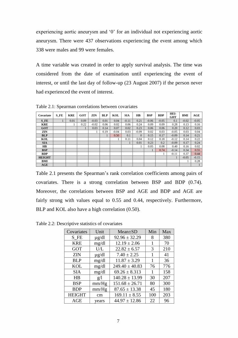
Table 2.1: Spearman correlations between covariates
Covariate S_FE KRE GOT ZIN BLP KOL SIA HB BSP BDP HEI-
GHT BMI AGE
S_FE 1 0.01 0.09 -0.03 0.01 0.04 -0.11 0.21 -0.06 -0.05 0.1 -0.02 -0.05
KRE 1 0.22 -0.02 0.06 0.02 0.06 0.24 0.09 0.09 0.28 0.13 0.16
GOT 1 0.03 0.14 0.07 0.02 0.23 0.06 0.06 0.20 0.12 0.03
ZIN 1 0.19 -0.04 0.03 -0.09 0.02 0.03 -0.05 0.03 0.04
BLP 1 0.50 0.1 0 0.15 0.17 -0.09 0.14 0.21
KOL 1 0.11 0.04 0.12 0.18 -0.12 0.14 0.22
SIA 1 0.01 0.23 0.2 -0.09 0.17 0.24
HB 1 0.05 0.08 0.40 0.16 0.02
BSP 1 0.74 -0.14 0.34 0.55
BDP 1 -0.11 0.37 0.44
HEIGHT 1 -0.05 -0.15
BMI 1 0.28
AGE 1
Table 2.1 presents the Spearman’s rank correlation coefficients among pairs of
covariates. There is a strong correlation between BSP and BDP (0.74).
Moreover, the correlations between BSP and AGE and BDP and AGE are
fairly strong with values equal to 0.55 and 0.44, respectively. Furthermore,
BLP and KOL also have a high correlation (0.50).
Table 2.2: Descriptive statistics of covariates
Covariates Unit Mean±SD Min Max
S_FE µg/dl 92.96 ± 32.29 8 380
KRE mg/dl 12.19 ± 2.06 1 70
GOT U/L 22.82 ± 6.57 3 210
ZIN µg/dl 7.40 ± 2.25 1 41
BLP mg/dl 11.87 ± 3.29 1 36
KOL mg/dl 249.40 ± 40.83 76 776
SIA mg/dl 69.26 ± 8.313 1 158
HB g/l 140.28 ± 13.99 30 207
BSP mm/Hg 151.68 ± 26.71 80 300
BDP mm/Hg 87.65 ± 13.38 45 180
HEIGHT cm 169.11 ± 8.55 100 203
AGE years 44.97 ± 12.86 22 96

8
3 Methods
3.1 Survival Analysis
Survival analysis contains a variety of statistical methods for analyzing time-to-
event data such as Cox regression analysis and Kaplan-Meier estimator. The
event is defined as a qualitative change with time and time is considered as the
length of time between the onset of the study and the occurrence of the event or
the last day of follow-up. A patient who survived during the follow-up period is
called right-censored which implies that the patient never experienced the event
of interest and the survival time is unknown (Collett, 2003).
Conventional models such as logistic regression are not suitable for this type of
data since they ignore information on the timing of event occurrence and do not
handle the censored cases (Allison, 2010).
3.1.1 Functions of survival time
3.1.1.1 The Survivor Function
The survivor function is defined as the probability that the survival time is
greater than or equal to time . In other words, it represents the probability that
an individual survives beyond a particular point of time. It can be written as:
is a particular point of time.
represents the time that the subject was observed on study.
Kaplan-Meier (KM) estimator is one method to estimate the survivor function
and it is the most widely used method. KM is also known as the product-limit
estimator and it is a non-parametric method. Both censored and uncensored
observations can be incorporated in the model (Hosmer and Lemeshow, 1999).
The KM estimator can be defined as:

9
is the number of individuals who are alive at time .
is the number of individuals who had died at time .
The main use of the KM estimator is for comparison of the survival patterns of
different subgroups. Comparing these patterns can be done by plotting the
survival curves from the KM estimator, which are shown as step-functions or
by using statistical tests such as the non-parametric Mantel-Haenszel test (or
log-rank test) and the Wilcoxon test. The Wilcoxon test is more suitable than
the log-rank test for comparing two survivor functions when the proportional
hazard assumption is violated (Collett, 2003).
3.1.1.2 The Hazard Function
Hazard ( ) is defined as the incidence rate or it can be called the mortality
rate when the outcome of interest is death at a particular point of time and it is
not assumed to be constant within time periods (Kirkwood and Sterne, 2003).
The cumulative hazard function, , is important in the identification of
models for survival data and it can be expressed as:
(Collett, 2003).
Hazard ratio, , is the ratio of hazards or cumulative hazards between
groups. Hazard ratio can be written in hazard values by 100(HR-1) and it can
be interpreted as the percentage change in hazard of the event for each
additional unit in that particular variable.
3.1.2 Cox Proportional Hazards Model
The Cox proportional hazards model is also known as Cox regression, which
was introduced by Sir David Cox in his famous paper “Regression Models and

10
Life Tables” (Cox, 1972). Cox regression has become one of the most common
frameworks for survival data analysis and making it the most highly cited
journal article in the entire literature of statistics (Allison, 2010). The model
can handle right-censoring and continuous time-event occurrence data by using
partial maximum likelihood estimation.
The proportional hazard model can be expressed as:
where is the dependent variable and is called the base line hazard
function when the value of all covariates are 0. The terms and
,…, are the covariates and regression coefficients, respectively. The
function represents the hazard function of the th individual at time . The
model can be re-expressed as:
The model is known as semi-parametric under the assumption that the hazard
ratio is constant over time.
The anti-logged coefficients will lead to the hazard ratio. Assume that two
individuals have different values on X. If the first individual has a value of
then and if the other has a value of then
. The hazard ratio then becomes:
Therefore, is the hypothesized constant hazard ratio for any one-unit
difference in the predictor, (Singer and Willett, 2003).
Cox regression can be used to make individual predictions of prognosis;
however, only few studies in the literature did (Jerez et al., 2005).
3.1.3 Cox Models with Non-Proportional Hazards
The proportional hazards (PH) assumption is that the effect of each covariate is
the same at all points in time; in other words, the hazard ratio between two

11
groups is constant over time. This assumption can be tested by using
Schoenfeld residuals. The Schoenfeld residuals are also known as partial
residuals and they have an important property: there is a separate residual for
each covariate for each individual. If the PH assumption holds, the Schoenfeld
residuals will be uncorrelated with time (Allison, 2010). Schoenfeld residuals
perform the best at detecting violations of the proportionality of hazards
(Singer and Willett, 2003). Violation of the PH assumption will lead to distort
effects. The effect of the violated PH assumption variable is an average effect
over a period of time (Allison, 2010).
Non-PH assumption can be treated by fitting interactions with time making a
model time-dependent or by stratification. The interaction between a covariate
and time is used if the covariate is of direct interest while stratification is used
for a covariate of indirect interest. The Cox model upon introducing the
interaction for a single time-invariant predictor X can be expressed as:
is the vertical displacement in log hazard associated with a one-unit
difference in X at time c.
represents how much vertical displacement is increased or decreased
with each one-unit increase in time.
(Singer and Willett, 2003).
The main effect of can be found when is 0 (at starting point). In
addition, the effect of for any can be calculated from
(Allison, 2010).
The other way to handle non-PH assumption is stratification. The model is
applied with a multiple baseline hazard function and can be expressed as:
The subscript in the equation indicates that each stratum has its own baseline
hazard function while the are the same across strata (Singer and Willett,
2003).

12
3.2 Continuation Ratio Model
The continuation ratio (CR) model is based on conditional probabilities. The
CR model can be express in this form:
(O'Connell, 2006).
The formula represents the conditional probability which the individual reach
beyond stage , given that the individual has reached stage . This model refers
to the analysis of a series of nested dichotomies (O'Connell, 2006).
The CR model will be useful when the ordered categories represent a
progression through different stages (Allison, 1999). If the response variable Y
is discrete survival times, the CR model represents a comparison of lower
survival times with higher survival times. The main assumption for the model
is that the effects of covariates are the same at each stage.
The data needs to be restructured in order to fit the CR model by using a binary
logistic model. The data set is divided into subsets. A new binary outcome
variable is created for each subset with ‘1’ representing a participant who
reaches that stage and ‘0’ representing a participant who does not reach that
stage. The individuals who do not survive until the next stage are dropped at
each stage. Then, these subsets are combined into one data set; therefore, a
restructured data set will be created and the number of observations will
increase. The restructured data set is conditionally independent (Armstrong &
Sloan, 1989); thus, the binary logistic regression can be used to analyze this
data set.
There are two famous link functions for fitting CR models, which are logit link
function and complementary log-log (clog-log) link function. The clog-log link
is concerned in this study since the time to the event is considered as a
continuous quantity. The clog-log is defined as:

13
The clog-log is showed as the log of negative log of the complementary
probability (O'Connell, 2006) and the clog-log link model is the discrete-time
equivalent of the proportional hazards model which is used in Cox regression
(McCullagh, 1980). The important benefits of using CR models are that the
ordinary logistic model can be used and it relaxes the equal-slopes assumption
which is the same as PH assumption (Harrell et al., 1998).
3.3 Logistic Regression
The logistic regression model is also known as the logit model, and it is a
generalization of linear regression. In medical research, binary logistic
regression is usually used, especially in order to find risk factors and this
method has become the common method of analysis for this situation (Hosmer
and Lemeshow, 2000). The response variable in binary logistic regression has
only two outcomes and refers to a binary or dichotomous response taking on
the values ‘0’ and ‘1’, which represent experiencing an event of interest and not
experiencing that event, respectively.
Let represents where is a set of covariates, i.e. the
conditional probability that the event of interest occur given values of the
predictors. The logit function or logit link of the logistic regression model is:
The logistic regression model can then be written as:
(Hosmer and Lemeshow, 2000)
re-written as:
The equation above shows that the values of will be between 0 and 1.
The maximum likelihood estimation is applied in order to find estimates of the

14
regression coefficients since OLS cannot handle the binary response (Allison,
1999).
The effects of covariates in logistic regression can be interpreted in three ways:
probabilities, odds, and logged odds. Odds are more frequent than the other two
because odds can express effects in single coefficients and have a
straightforward interpretation (Pampel, 2000). The odds are defined as:
The odds ratio is the ratio of odds for comparing one group with a reference
group, for example, comparing the odds of experiencing aortic aneurysm
between males and females. Let and be the probabilities of the
event of interest for males and females, respectively. The odds ratio can be
defined as:
OR = 1: males and females have the same odds of the event of interest.
OR > 1: males are more likely to experience the event of interest than
females.
OR < 1: females is more likely to experience the event of interest than
males
Then, the percent of change in odds for each unit increase in the covariate is
obtained by calculating:
(Pampel, 2000).
The odds ratio can be obtained by taking exponential functions of the
regression coefficient:

15
3.4 Decision Tree
Decision trees are reliable and effective decision making techniques that
provide high classification accuracy with a simple representation of gathered
knowledge and they have been used in different areas of medical decision
making (Podgorelec et al, 2002). A decision tree model consists of a set of
rules for dividing a large heterogeneous population into smaller, more
homogeneous groups with respect to a particular target variable. The advantage
is that the results can be understood and explained easily because a tree
structured diagram is easy to interpret. The input and target can be both
categorical and continuous variables. However, a categorical response variable
is usually used and the model is called a classification tree. The decision tree
will calculate for each of the categories the probability that a given record
belongs to that category.
The process of a decision tree begins at the root node and works from top to
down. When an observation enters the tree at the root node then the root node
applies a test to find which child node the observation will go next. The test is
based on the best discriminates among the target classes. Repeating this process
until the observation reaches a leaf node defines the classification.
The classification and regression tree (CART) method is a widely known
algorithm in tree modeling. CART method determines the best possible binary
splits and the binary splits performed are based on nominal or interval input
variables.
Splitting Criterion
The splitting criterion measures the decrease in the distribution of the target
variable between the root node and the first subsequent node and between each
pair of subsequent nodes. The splitting criterion has two objectives: to
determine the best split for each input variable and to choose the best split

16
among a multitude of possible splits from input variables. For classification
trees, there are two common splitting criterions, which are Gini index and
entropy reduction.
1. Gini index (Total Leaf Impurity)
Gini index is a measure of purity. If the target values are the same
within the node then the Gini index is one. The best split is selected by
the largest Gini index. The Gini index can be calculated as follows:
is the Gini index at node .
is the proportion of each target class in the node.
= number of individuals in the leaf node / total number of
individuals in node .
(Matignon, 2007).
2. Entropy reduction
Entropy reduction is a measure of variability in categorical data.
If the target values are the same within the node then the entropy is zero.
Thus, the best split is selected by the smallest entropy reduction. The
Entropy reduction is defined as:
is the proportion of each target class in corresponding node .
(Matignon, 2007).

17
3.5 Artificial Neural Networks
An Artificial Neural Network, or simply neural network, is a nonparametric
model which is useful when the relationship between inputs and outputs are
nonlinear. Neural network is the most popular artificial intelligence-based data
modeling algorithm used in clinical medicine for diagnosis of diseases
(Bellazzi and Zupan, 2008).
A neural network consists of three or more layers which are an input layer, one
or more hidden layers, and an output layer. Moreover, a neural network is like a
regression model in these aspects: covariates are called ‘inputs’, coefficients
are called ‘weights’ and outcome variables are known as ‘output (Berry and
Linoff, 2004).
Figure 3.1: Three layer feed-forward neural network showing the information process.
A feed-forward neural network calculates output values from input values.
Each neuron in one layer is connected to every neuron in the next layer and the
signals flow only in one direction across the network as shown in Figure 3.1.
This type of network is used for prediction and classification.
The training of a neural network is the process to obtain the best weights on the
edges connecting all the units in the network. The training set is used to
calculate weights where the output gives the most desired response as possible.
The back-propagation, which is a so-called supervised learning network, is
used for adjusting weights and it has been used widely in the medical literature
(Ohno-Machado, 1996). The back-propagation measures the overall errors of
the network by comparing the produced values with the actual values in the
Input 1
Input 2
Input 4
Input 3
Output
4

18
training set. The adjusted weights are calculated to reduce the error in the
output. Moreover, the back-propagation can be used without any assumption
about distributed relationships. The feed-forward artificial neural network
model where the back-propagation algorithm is used is called a multi-layer
perception (MLP).
A single hidden layer is sufficient for classification problems. The use of a
second hidden layer is to reduce the number of hidden nodes on the first hidden
layer (Ozkan and Erbek, 2003). However, it depends on the complexity of the
dataset.
Each hidden node has its own activation function. The activation function has
two parts: the combination function and the transfer function. The first part, the
combination function, merges all inputs into a single value by using a weighted
sum. The weighted sum is calculated by multiplying each input with its weight
and then adding these products together. The second part is the transfer
function which transfers the value from the first part to the output node. When
using the back-propagation network, the transfer function must be
differentiable; therefore, the function is bounded to certain ranges of limits.
Common transfer functions used in MLP are the standard logistic sigmoid and
the hyperbolic tangent transfer function. The standard logistic sigmoid function
has a range between 0 and 1 and is S-shaped. The hyperbolic tangent transfer
function is similar to the standard logistic sigmoid function in transforming the
values to the output class between -1 and 1 and it also has the S-shape. The
sigmoid function shows both linear and non-linear behavior. The hyperbolic
tangent function has an advantage over the standard logistic sigmoid function,
in that it performs a faster convergence (Crespo et al., 2001).

19
3.6 Receiver Operating Characteristics curves
The Receiver Operating Characteristics (ROC) curve was originally introduced
in signal detection theory in connection with the study of radio signals (Zweig
M. H., & Campbell G, 1993). ROC analysis has been used in medicine,
radiology, biometrics and other areas since then. Moreover, ROC analysis
becomes more famous in medicine learning and data mining research.
ROC curves are used in medicine to determine a cutoff value for a clinical test,
i.e. a value above which the test says the result is positive. The ROC curve is a
graphical representation of the tradeoff between the true positive rates and the
false negative rates for every possible cut-off. Equivalently, the ROC curve is a
plot that displays the picture of tradeoff between the sensitivity (true positive
rate) and (1-specificity) (false positive rate) across a series of cut-off points.
Table 3.1: Reporting accuracy for binary prediction
Forecast Observed
Positive Negative
Positive True Positive (TP) False Positive (FP)
Negative False Negative (FN) True Negative (TN)
The different fractions: TP, FP, TN, and FN are represented in Table 3.1. The
sensitivity and specificity can be expressed as:
The sensitivity of a diagnostic test is the proportion of patients for whom the
outcome is positive that are correctly identified by the test (Bewick et al.,
2004). The specificity is the proportion of patients for whom the outcome is
negative that are correctly identified by the test (Bewick et al., 2004).
Moreover, sensitivity and specificity are the most common way to report the
accuracy of a binary prediction (GÖnen, 2007).

20
A good diagnostic test is one that has small false positive and false negative
rates across a reasonable range of cut off values. If the ROC curve climbs
rapidly towards the upper left corner of the graph, this means that the true
positive rate is high and the false positive rate is low. An accuracy
measurement, misclassification rate, is a popular test in machine learning to
measure how well the methods work; however, it is not acceptable in medical
(Cios and Moore, 2002). The concept of Area Under the Curve (AUC) is
introduced and it is considered as an effective measure of inherent validity of a
diagnostic test. Furthermore, the AUC is the most commonly used statistics for
summarizing the ROC curve.
The larger area is the better diagnostic test. If the area is 1.0, then it is an ideal
test because it achieves both 100% sensitivity and 100% specificity. If the area
is 0.5, then a test has effectively 50% specificity and 50% specificity. The
closer the area is to 1.0, the better the test is and the closer the area is to 0.5, the
worse the test is. The ROC curve is useful in these followed aspects:
Evaluation of the discriminatory ability of a test to correctly predict.
Finding optimal cut-off point that gives the lowest misclassification of
the health outcome.
Comparing efficacy of two or more medical tests for predicting the
same health outcome.

21
4 Results
Find Risk Factors Part
4.1 Survival Analysis
4.1.1 The Cox Regression Model
Cox regression model is used to find significant risk factors by applying Wald
Chi-Square tests to determine the influence of each covariate on the response
variable. The set of covariates are chosen from automatic selection methods
mentioned in Chapter 3. All of them yield the same set of covariates. The set of
covariates consist of AGE, SEX, BDP, KOL, BLP, SIA, HEIGHT,
URIN_SOC, GOT and BSP.
Figure 4.1: Wald Chi-Square values for each risk factor in the Cox regression model.
Figure 4.1 shows the Wald Chi-Square values of the risk factors for the Cox
regression model. The dashed line represents the Chi-Square value with 5%
significance level and one degree of freedom which equal to 3.84. The higher
Wald Chi-Square value indicates the more covariate contributes to the model.
The Cox regression model indicates that AGE is the most significant covariate
and that is expected since getting older tends to experience a lot of diseases.
SEX also has a strong significance. BDP, KOL, and BLP are found as
22
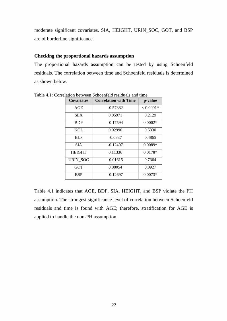
moderate significant covariates. SIA, HEIGHT, URIN_SOC, GOT, and BSP
are of borderline significance.
Checking the proportional hazards assumption
The proportional hazards assumption can be tested by using Schoenfeld
residuals. The correlation between time and Schoenfeld residuals is determined
as shown below.
Table 4.1: Correlation between Schoenfeld residuals and time
Covariates Correlation with Time p-value
AGE -0.57382 < 0.0001*
SEX 0.05971 0.2129
BDP -0.17594 0.0002*
KOL 0.02990 0.5330
BLP -0.0337 0.4865
SIA -0.12497 0.0089*
HEIGHT 0.11336 0.0178*
URIN_SOC -0.01615 0.7364
GOT 0.08054 0.0927
BSP -0.12697 0.0073*
Table 4.1 indicates that AGE, BDP, SIA, HEIGHT, and BSP violate the PH
assumption. The strongest significance level of correlation between Schoenfeld
residuals and time is found with AGE; therefore, stratification for AGE is
applied to handle the non-PH assumption.

23
Figure 4.2: Wald Chi-Square values for each risk factor in the Cox regression model
after stratification.
Figure 4.2 illustrates the comparison of the Wald Chi-Square values for Cox
regression model with AGE stratification. SEX is the most significant
covariate. The relatively strong significant covariates are BDP and BLP while
KOL and SIA have a moderate significance. HEIGHT GOT, URIN_SOC, and
BSP are at borderline significance; thus, they are not the main interesting
covariates.
The correlation between time and Schoenfeld residuals are determined one
more time in order to check non-PH assumption. Table 4.2 presents that none
of the covariates violates the PH assumption. Furthermore, the hazard ratios for
each covariate in the Cox regression after stratification are shown in Table 4.3.
Table 4.2: Correlation between Schoenfeld residuals and time
Covariates Correlation with Time p-value
SEX 0.04380 0.3610
BDP -0.02833 0.5547
BLP 0.04022 0.4017
KOL 0.08914 0.0626
SIA -0.04950 0.3019
HEIGHT 0.04590 0.3385
GOT 0.06072 0.2052
URIN_SOC 0.00778 0.8711
BSP 0.05381 0.2616

24
Table 4.3: Results of Cox regression after stratification
Table 4.3 shows that the hazard ratio for SEX was 3.547, which means that the
hazard of experiencing aortic aneurysm in males is 3.548 times greater than in
females and the 95 percent confidence interval was from 2.609 to 4.824 times.
The hazard for BDP indicates that each additional unit (mm/Hg) of BDP
increased the hazard of experiencing aortic aneurysm by 2.7 percent and the 95
percent CI is from 1.6 to 3.8 percent. For each additional unit (mg/dl) of BLP,
the hazard of contacting aortic aneurysm increases by 6.6 percent with the 95
percent CI from 3.4 to 10 percent. Each Increasing unit (mg/dl) of KOL, hazard
increases by 0.5 percent with a possible range from 0.2 to 0.7 percent. The
hazard for SIA shows that each additional unit (mg/dl) of SIA increases the
hazard by 1.9 percent and 95 percent CI is from 0.8 to 3.1 percent. For each
extra unit (U/L) in GOT, the hazard decreases 0.02 percent with possible range
from 0.004 to 0.037 percent.
The hazard ratio is normally interpreted with one unit increase in that covariate;
however, one unit change may be too small to see the effect of some covariates.
For example, the hazard of a 10 unit (mm/HG) increase in BDP increases the
hazard by 30.64 ( ) percent. A 5 unit (cm) increase in HEIGHT
increases the hazard of experiencing aortic aneurysm by 10.99 ( )
percent.
Covariates Coefficient Hazard
Ratio
95% CI
Lower
Bound
95% CI
Upper
Bound
p-value
SEX 1.2661 3.548 2.609 4.824 <0.0001
BDP 0.0267 1.027 1.016 1.038 <0.0001
BLP 0.0642 1.066 1.034 1.1 <0.0001
KOL 0.0048 1.005 1.002 1.007 0.0003
SIA 0.0192 1.019 1.008 1.031 0.0009
HEIGHT 0.0209 1.021 1.005 1.037 0.0097
GOT -0.0204 0.98 0.963 0.996 0.018
URIN_SOC -2.0287 0.13 0.018 0.929 0.042
BSP -0.0059 0.994 0.988 1 0.0498
25
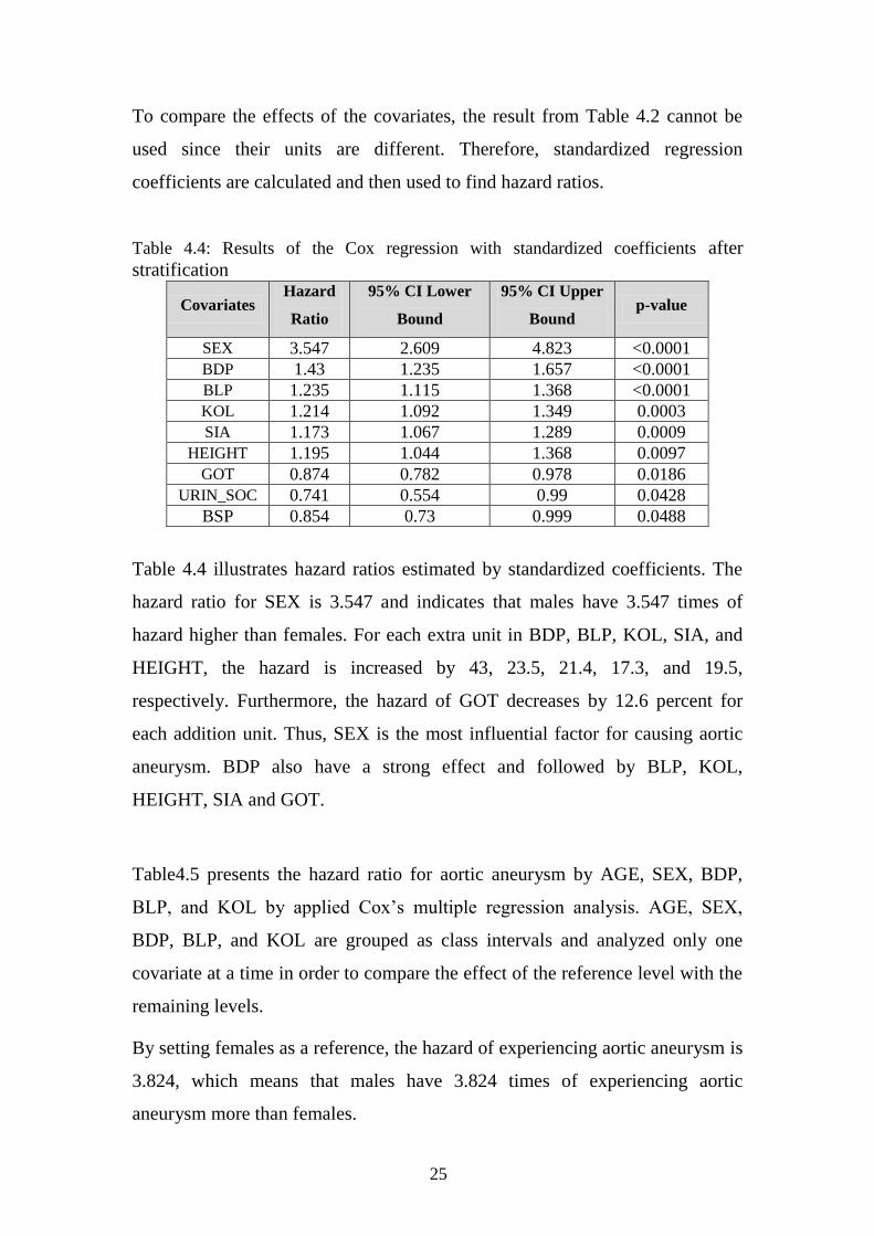
To compare the effects of the covariates, the result from Table 4.2 cannot be
used since their units are different. Therefore, standardized regression
coefficients are calculated and then used to find hazard ratios.
Table 4.4: Results of the Cox regression with standardized coefficients after
stratification
Table 4.4 illustrates hazard ratios estimated by standardized coefficients. The
hazard ratio for SEX is 3.547 and indicates that males have 3.547 times of
hazard higher than females. For each extra unit in BDP, BLP, KOL, SIA, and
HEIGHT, the hazard is increased by 43, 23.5, 21.4, 17.3, and 19.5,
respectively. Furthermore, the hazard of GOT decreases by 12.6 percent for
each addition unit. Thus, SEX is the most influential factor for causing aortic
aneurysm. BDP also have a strong effect and followed by BLP, KOL,
HEIGHT, SIA and GOT.
Table4.5 presents the hazard ratio for aortic aneurysm by AGE, SEX, BDP,
BLP, and KOL by applied Cox’s multiple regression analysis. AGE, SEX,
BDP, BLP, and KOL are grouped as class intervals and analyzed only one
covariate at a time in order to compare the effect of the reference level with the
remaining levels.
By setting females as a reference, the hazard of experiencing aortic aneurysm is
3.824, which means that males have 3.824 times of experiencing aortic
aneurysm more than females.
Covariates Hazard
Ratio
95% CI Lower
Bound
95% CI Upper
Bound p-value
SEX 3.547 2.609 4.823 <0.0001
BDP 1.43 1.235 1.657 <0.0001
BLP 1.235 1.115 1.368 <0.0001
KOL 1.214 1.092 1.349 0.0003
SIA 1.173 1.067 1.289 0.0009
HEIGHT 1.195 1.044 1.368 0.0097
GOT 0.874 0.782 0.978 0.0186
URIN_SOC 0.741 0.554 0.99 0.0428
BSP 0.854 0.73 0.999 0.0488

26
Table 4.5: Hazard ratio for aortic aneurysm by class variables
Covariates No. of
cases Participants
Hazard
Ratio 95% CI p-value
SEX
Female
Male
99
338
30,343
33,501
1 (Ref)
3.824
-
(3.053,4.789)
-
<0.0001
BDP (mm/Hg)
Normal(<80)
Pre-hypertension(80 -89)
Stage1 of hypertension(90 - 99)
Stage2 of hypertension(≥100)
135
28
169
105
26,353
5,812
18,687
12,992
1 (Ref)
0.880
1.665
1.69
-
(0.585,1.324)
(1.317,2.098)
(1.281,2.231)
-
0.5395
<0.0001
0.0002
BLP (mg/dl)
<10
10-11
12-13
≥14
59
115
97
166
14,906
17,723
13,802
17,413
1 (Ref)
1.566
1.624
2.181
-
(1.143,2.144)
(1.176,2.249)
(1.611,2.952)
-
0.0052
0.0035
<0.0001
KOL (mg/dl)
Normal(<200)
Moderate(200 – 239)
High(≥240)
15
107
315
5812
19327
38705
1 (Ref)
1.894
2.582
-
(1.103,3.254)
(1.532,4.352)
-
0.0207
0.0004
BDP is separated into four levels and normal BDP is set as a reference. Stage 1
of hypertension group increases the hazard of experiencing aortic aneurysm by
66.5 percent when compared to the reference group with a strong significance
level. Moreover, stage 2 of hypertension group also raised the hazard by 69
percent.
BLP is split into four groups. The first group of BLP (<10 mg/dl) is set as a
reference group. The second BLP group (10-11 mg/dl) increases the hazard of
experiencing aortic aneurysm by 56.6 percent comparing to the reference
group. Moreover, the third and last BLP groups raise the hazard of contacting
aortic aneurysm by 62.4 and 118.1 percent.
KOL is divided into three groups and normal level of KOL is set as a reference
level. KOL levels are linked with an increased risk of aortic aneurysm.
Moderate level of KOL yields 89.4 percent higher hazard than the reference
level. In addition, high level of KOL increases the hazard of causing aortic
aneurysm by 158.2 percent with a strong significance level.

27
4.1.2 The Kaplan-Meier Estimator
Covariate: SEX
Figure 4.3: The Kaplan-Meier estimator of the survival function with SEX
The survival plot is applied to show the difference between males and females.
Figure 4.3 illustrates that the survival curve starts to separate between males
and females after 2 years of follow-up. Furthermore, it is obvious that males
experienced more aortic aneurysm than females after 20 years of follow-up.
Table 4.6: Results of log-rank test and Wilcoxon test across the strata for SEX
Test Chi-Square DF p-value
Log-Rank 161.3247 1 <0.0001
Wilcoxon 144.0426 1 <0.0001
Table 4.6 displays non-parametric test which are log-rank and Wilcoxon test
and both of them are confirmed that the survival curves of male and female are
strongly different.
Covariate: BDP
BPD is separated into two groups: normal BDP group (<80 mm/Hg) and
elevated BDP group (>=80 mm/Hg). Figure 4.4 shows the survival curves

28
which diverged significantly. The statistics tests confirm this result as well
which is presented in Table 4.7.
Figure 4.4: The Kaplan-Meier estimator of the survival function with BDP
Table 4.7: Results of log-rank test and Wilcoxon test across the strata for BPD
Test Chi-Square DF p-value
Log-Rank 47.1818 1 <0.0001
Wilcoxon 50.9647 1 <0.0001
Covariate: BLP
BLP is divided into two groups which are normal BLP group (<12 mg/dl) and
elevated BLP group (≥12 mg/dl). Figure 4.5 shows the survival curves which
slightly diverge through time and the curves diverge significantly in later years.
The tests of homogeneity of strata in Table 4.8 also suggest that the survival
curves of two strata are different with a strong significant level.

29
Figure 4.5: The Kaplan-Meier estimator of the survival function with BLP
Table 4.8: Results of log-rank test and Wilcoxon test across the strata for BLP
Test Chi-Square DF p-value
Log-Rank 53.1027 1 <.0001
Wilcoxon 50.6147 1 <.0001
Covariate: KOL
Figure 4.6: The Kaplan-Meier estimator of the survival function with KOL
KOL is divided into two groups: normal KOL group (<200 mg/dl) and elevated
KOL group (≥200mg/dl). The survival curves for KOL is shown in figure 6 and
it illustrates that the curves diverge significantly. The statistics tests in Table

30
4.9 also confirm that normal KOL group and elevated KIOL group do not have
the same survivor function.
Table 4.9: Results of log-rank test and Wilcoxon test across the strata for KOL
Test Chi-Square DF p-value
Log-Rank 25.1938 1 <0.0001
Wilcoxon 25.7662 1 <0.0001
4.1.3 Subgroup Analysis
Male Subgroup
Cox regression is one again applied to find risk factors in the male subgroup.
The automatic selection methods yield the same set of covariates which consist
of AGE, BDP, KOL, BLP, HEIGHT, GOT, URIN_SOC, and SIA.
Figure 4.7: Wald Chi-Square values for each risk factor among the male subgroup
with the
The most significant covariate is AGE. BDP, KOL, BLP, and HEIGHT are
moderately significant while GOT, URIN_SOC, and SIA are at borderline
significance.
Checking the proportional hazards assumption
The correlation between time and Schoenfeld residuals are determined in order
to check non-PH assumption.
31
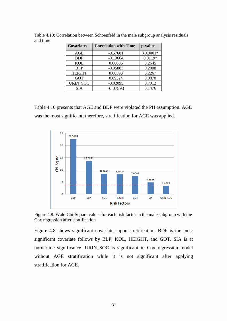
Table 4.10: Correlation between Schoenfeld in the male subgroup analysis residuals
and time
Covariates Correlation with Time p-value
AGE -0.57681 <0.0001*
BDP -0.13664 0.0119*
KOL 0.06086 0.2645
BLP -0.05883 0.2808
HEIGHT 0.06593 0.2267
GOT 0.09324 0.0870
URIN_SOC -0.02095 0.7012
SIA -0.07893 0.1476
Table 4.10 presents that AGE and BDP were violated the PH assumption. AGE
was the most significant; therefore, stratification for AGE was applied.
Figure 4.8: Wald Chi-Square values for each risk factor in the male subgroup with the
Cox regression after stratification
Figure 4.8 shows significant covariates upon stratification. BDP is the most
significant covariate follows by BLP, KOL, HEIGHT, and GOT. SIA is at
borderline significance. URIN_SOC is significant in Cox regression model
without AGE stratification while it is not significant after applying
stratification for AGE.

32
Female Subgroup
Figure 4.9 displays the comparison of the Wald Chi-Square values when
applying the Cox regression model to the female subgroup. The most
significant covariate is AGE. BDP, SIA, BSP, and KOL are moderately
significant while BLP is at borderline significance.
Figure 4.9: Wald Chi-Square values for each risk factor in the female subgroup with
the Cox regression
Checking the proportional hazards assumption
Table 4.11 presents that AGE, BDP, and SIA are violated the PH assumption.
AGE is the most strongly significant; therefore, stratification for AGE is
applied.
Table 4.11: Correlation between Schoenfeld residuals in the female subgroup analysis
and time Covariates Correlation with Time p-value
AGE -0.55501 <0.0001*
BDP -0.28760 0.0039*
SIA -0.25575 0.0106*
BSP -0.20371 0.0431*
KOL -0.02815 0.7821
BLP 0.09005 0.3754
Figure 4.10 illustrates that SIA is the most significant covariate for female
subgroup and follows by BDP and BSP. KOL and BLP are significant in the
Cox regression model without AGE stratification while they are not significant
upon stratification for AGE.

33
Figure 4.10: Wald Chi-Square values for each risk factor in the female subgroup with
the Cox regression after stratification
Table 4.12: Hazard ratio by BDP and KOL in the male and female subgroup
Covariates
Male (n = 33,481 with 338 events) Female (n = 30,331 with 99 events)
No. of
cases
Partici-
pants HR 95% CI p-value
No. of
cases
Partici
-pants HR 95% CI p-value
BDP (mm/Hg)
Normal(<80)
Pre-hypertension
Stage1 of hypertension
Stage2 of hypertension
107
23
125
83
13600
3246
10274
6361
Ref.
0.901
1.642
2.229
-
(0.574,1.415)
(1.262,2.136)
(1.639,3.031)
-
0.6508
0.0009
<0.0001
28
5
44
22
12722
2566
8413
6631
Ref.
0.742
1.876
1.210
-
(0.285,1.930)
(1.145,3.081)
(0.653, 2.242)
-
0.5402
0.0129
0.5446
KOL (mg/dl)
Normal (<200)
Moderate (200 - 239)
High (≥240)
12
91
235
3105
10231
20145
Ref.
2.117
2.756
-
(1.159, 3.868)
(1.538, 4.940)
-
0.0148
0.0007
3
16
80
2701
9088
18542
Ref.
1.343
2.738
-
(0.391, 4.619)
(0.853, 8.788)
-
0.6398
0.0905
Note: Ref. means the reference group
Table 4.12 presents hazard ratios of BDP and KOL which are examined by
SEX. Cox’s multiple regression models is applied only one variable at a time
with adjusted AGE, BDP and KOL as class variables. The class variables are
used in order to compare the effect of BDP and KOL between the reference
(normal) group and the remaining groups.
The stage 1 of the hypertension group increases the hazard of experiencing
aortic aneurysm by 64.2 percent and 87.6 percent in the male and the female
group, respectively. In addition, the hazard of contacting aortic aneurysm for
having stage 2 of hypertension is raised by 122.9 percent in males.
The moderate KOL group and the high KOL group increase the hazard of
experiencing aortic aneurysm by 111.7 and 175.6 percent in male, respectively.
However, any of KOL group is significant in the female subgroup.

34
Cox’s multiple regression is carried out again in order to compare the risk
factors between males and females. BDP, BLP, KOL, SIA, HEIGHT, and GOT
are fixed in the model to find the different effect between male and female
group.
Table 4.13: Hazard ratio by fixed covariates in the male and female subgroup
Covariates Male (n = 33,481 with 338 events) Female (n = 30,331 with 99 events)
HR 95% CI p-value HR 95% CI p-value
BDP (mm/Hg) 1.022 (1.013, 1.031) <0.0001 1.008 (0.992,1.024) 0.3214
BLP (mg/dl) 1.068 (1.031,1.106) 0.0003 1.066 (0.999,1.137) 0.0538
KOL (mg/dl) 1.004 (1.001,1.008) 0.0036 1.005 (1.000, 1.010) 0.0594
SIA (mg/dl) 1.015 (1.001,1.028) 0.0323 1.031 (1.007,1.055) 0.0101
HEIGHT (cm) 1.026 (1.008,1.044) 0.0040 0.999 (0.964,1.036) 0.9771
GOT (U/L) 0.974 (0.955,0.993) 0.0067 0.995 (0.959,1.034) 0.8115
Table 4.13 shows hazard ratios and p-values for aortic aneurysm in the male
and the female groups and it discloses that BDP, BLP, KOL, HEIGHT and
GOT are strongly significant only in the male subgroup. The hazard ratios for
SIA are slightly different between the males and the females.
Age groups
The dataset is divided age at examination into six age groups in order to reveal
risk factors for each age group. The first age group contains participants who
aged up to 45 years old. The second age group consists of participants aged
from 46 to 55 years old. The third age group has ages form 56 to 65 years old.
The last age group has ages over 65 years old. Table 4.14 illustrates the number
of aortic aneurysm in male and female for each age group.
35
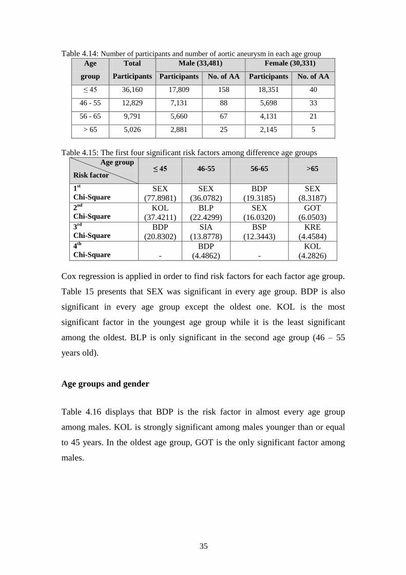
Table 4.14: Number of participants and number of aortic aneurysm in each age group
Age
group
Total
Participants
Male (33,481) Female (30,331)
Participants No. of AA Participants No. of AA
≤ 45 36,160 17,809 158 18,351 40
46 - 55 12,829 7,131 88 5,698 33
56 - 65 9,791 5,660 67 4,131 21
> 65 5,026 2,881 25 2,145 5
Table 4.15: The first four significant risk factors among difference age groups
Age group
Risk factor ≤ 45 46-55 56-65 >65
1st
Chi-Square SEX
(77.8981)
SEX
(36.0782)
BDP
(19.3185)
SEX
(8.3187)
2nd
Chi-Square KOL
(37.4211)
BLP
(22.4299)
SEX
(16.0320)
GOT
(6.0503)
3rd
Chi-Square BDP
(20.8302)
SIA
(13.8778)
BSP
(12.3443)
KRE
(4.4584)
4th
Chi-Square -
BDP
(4.4862)
-
KOL
(4.2826)
Cox regression is applied in order to find risk factors for each factor age group.
Table 15 presents that SEX was significant in every age group. BDP is also
significant in every age group except the oldest one. KOL is the most
significant factor in the youngest age group while it is the least significant
among the oldest. BLP is only significant in the second age group (46 – 55
years old).
Age groups and gender
Table 4.16 displays that BDP is the risk factor in almost every age group
among males. KOL is strongly significant among males younger than or equal
to 45 years. In the oldest age group, GOT is the only significant factor among
males.

36
Table 4.16: The first four significant risk factors in male subgroup and age groups
Age group
Risk factor ≤ 45 46-55 56-65 >65
1st
Chi-Square KOL
(30.2782)
BLP
(13.4148)
BDP
(12.8278)
GOT
(6.7013)
2nd
Chi-Square BDP
(18.9889)
BDP
(6.119)
BSP
(7.2685) -
3rd
Chi-Square -
HEIGHT
(5.4302) - -
4th
Chi-Square -
SIA
(5.2067)
- -
Table 4.17: The first four significant risk factors in female subgroup and age groups
Age group
Risk factor ≤ 45 46-55 56-65 >65
1st
Chi-Square KOL
(8.3037)
SIA
(13.8386)
BDP
(6.5565)
HB
(4.3225)
2nd
Chi-Square -
BLP
(11.4705)
BSP
(5.5519)
KRE
(4.1842)
3rd
Chi-Square -
HB
(5.7807) - -
4th
Chi-Square - -
- -
KOL is found as significant risk factor in the youngest age group among
females. For third age group (56- 65 years old), the significant risk factors
among males and females yield the result which are BDP and BSP. In the
oldest age group, HB and KRE are significant risk factors among females.
Thus, the most three important risk factors are KOL, BLP, and blood pressure
in both the male and the female group.

37
4.2 The Continuation Ratio Model
The Continuation ratio model is applied to find significant risk factors in order
to compare the result with the Cox regression. One of the advantages is that it
is possible to work with the general model which is logistic regression by
restructuring the dataset. The set of significant covariates consist of SEX, BDP,
BSP, KOL, BLP, HEIGHT, URIN_SOC, AGE and GOT as shown in Figure
4.11.
Figure 4.11: Wald Chi-Square values for each risk factor in the continuation ratio
model
Figure 4.11 shows that SEX is strongly significant follow by BDP and BSP.
KOL, BLP, and HEIGHT have a moderate significance whereas HEIGHT,
URIN_SOC, and AGE are slightly significant. GOT is at borderline
significance.
Table 4.18: Results of the continuation ratio model
Covariates Hazard
Ratio
95% CI
Lower Bound
95% CI Upper
Bound p-value
SEX 1.557 1.441 1.683 <0.0001
BDP 1.025 1.019 1.03 <0.0001
BSP 0.989 0.986 0.992 0.0002
KOL 1.005 1.003 1.006 0.0002
BLP 1.06 1.043 1.077 0.0002
HEIGHT 1.027 1.019 1.035 0.0008
URIN_SOC 0.08 0.029 0.218 0.0117
AGE 1.012 1.007 1.017 0.0089
GOT 0.983 0.975 0.991 0.0387

38
Table 4.18 shows the hazard ratios for the CR model. The hazard of
experiencing aortic aneurysm in males is 55.7 percent greater than in females.
Increasing one unit (mg/Hg) of BDP, hazard increases by 2.5 percent and the
95 percent CI is from 1.9 to 3 percent. The hazard for BSP informs that each
extra unit (mg/Hg) in BSP decreases the hazard of contacting aortic aneurysm
by 1.1 percent with the 95 percent CI from 0.14 to 0.8 percent.
The hazard of KOL increases by 0.5 percent for each additional unit (mg/dl)
and the 95 percent CI is from 0.3 to 0.6 percent. The hazard for BLP indicates
that each additional unit (mg/dl) of BLP increases the hazard by 6 percent with
the 95 percent CI from 4.3 to 7.7 percent.
For each increasing unit (cm) in HEIGHT, the hazard raises 2.7 percent with
the 95 percent from 1.9 to 3.5 percent. The obtained hazard ratio of
experiencing aortic aneurysm for having URIN_SOC relative to not having
URIN_SOC was 0.08. It can be indicated that having URIN_SOC had 92
percent lower hazard of experiencing aortic aneurysm than not having
URIN_SOC and the 95 percent CI was from 78.2 to 97.1 percent.
The hazard for AGE indicates that each additional unit (year) of AGE increases
the hazard by 1.2 percent with the 95 percent CI from 0.7 to 1.7 percent.
Raising one unit (U/L) of GOT results that, the hazard decreases by 1.7 percent
with the 95 percent CI from 0.9 to 2.5 percent.
Both of the blood pressure measurements are strongly significant but the effects
have different directions. The difference between BSP and BDP (diffBP) is
calculated and added to the model for an explanation. The CR model is applied
once again by using diffBP instead of BSP.

39
Table 4.19: Results of the continuation ratio model
The hazard of experiencing aortic aneurysm is decreased by 1.1 percent for
each additional unit (mm/Hg) of diffBP with the 95 percent CI from 0.8 to 1.4
percent as shown in Table 4.19.
4.2.1 Subgroup Analysis
Male subgroup
The CR model is carried out in order to find the risk factors in the male
subgroup. The set of significant risk factors consist of BDP, HEIGHT, BLP,
BSP, KOL, URIN_SOC, and GOT. Figure 4.12 shows that BDP and HEIGHT
are the strongly significant. BSP and KOL are moderate significance while
URIN_SOC and GOT are at borderline significance.
Figure 4.12: Wald Chi-Square values for each risk factor among the male subgroup in
the continuation ratio model
Covariates Hazard
Ratio
95% CI
Lower Bound
95% CI
Upper Bound p-value
SEX 1.557 1.441 1.683 <0.0001
BDP 1.013 1.009 1.017 0.0011
diffBP 0.989 0.986 0.992 0.0002
KOL 1.005 1.003 1.006 0.0002
BLP 1.06 1.043 1.076 0.0002
HEIGHT 1.027 1.019 1.035 0.0008
URIN_SOC 0.08 0.029 0.218 0.0117
AGE 1.012 1.007 1.017 0.0089
GOT 0.983 0.975 0.991 0.0387

40
Table 4.20: Results of the continuation ratio model among the male subgroup
Female subgroup
There are 4 significant covariates in the female group which are BDP, BSP,
KOL, and AGE. Figure 4.13 illustrates that BDP is the strongest significant
covariate where as BSP, KOL, and AGE are moderately significant.
Figure 4.13: Wald Chi-Square values for each risk factor among the female subgroup
in the continuation ratio model
BDP, BSP and KOL are significant in both the male and the female subgroups.
However, these three covariates have stronger effects among males than among
females. On the other hand, HEIGHT, BLP, URIN_SOC, and GOT are only
significant in the male subgroup and AGE is only significant in the female
subgroup.
Table 4.21: Results of the continuation ratio model among the female subgroup
Covariates Hazard
Ratio
95% CI
Lower Bound
95% CI
Upper Bound p-value
BDP 1.023 1.016 1.029 0.0004
HEIGHT 1.032 1.023 1.041 0.0004
BLP 1.062 1.043 1.082 0.0012
BSP 0.991 0.987 0.994 0.0075
KOL 1.004 1.003 1.006 0.0083
URIN_SOC 0.099 0.036 0.268 0.0208
GOT 0.979 0.97 0.988 0.0253
Covariates Hazard
Ratio
95% CI
Lower Bound
95% CI
Upper Bound p-value
KOL 1.008 1.006 1.01 <0.0001
BSP 0.98 0.974 0.986 0.0013
BDP 1.033 1.021 1.045 0.0046
AGE 1.026 1.016 1.037 0.0082

41
4.3 The Logistic Regression Model
Logistic Regression is applied in order to find the risk factors in order to
compare the result with the Cox regression and the continuation ratio model.
The automatic selection methods, which are forward, backward, and stepwise
yield the same set of covariates. The set of covariates consist of SEX, BDP,
BSP, KOL, HEIGHT, AGE, URIN_SOC, and GOT.
Figure 4.14 shows that SEX and BDP are strongly significant. BSP, KOL,
BLP, and HEIGHT have a moderate significance whereas HEIGHT,
URIN_SOC, and AGE are slightly significant. GOT is at borderline
significance.
Figure 4.14: Wald Chi-Square values for each risk factor in the logistic regression
model
Table 4.22: Results of the logistic regression model
Covariates Odds
Ratio
95% CI
Lower Bound
95% CI
Upper Bound p-value
SEX 2.434 1.794 3.301 <0.0001
BDP 1.025 1.014 1.036 <0.0001
BSP 0.989 0.983 0.995 <.0001
BLP 1.005 1.002 1.007 0.0002
KOL 1.06 1.028 1.094 0.0002
HEIGHT 1.027 1.011 1.043 0.0002
AGE 1.012 1.003 1.021 0.0008
URIN_SOC 0.079 0.011 0.566 0.008
GOT 0.983 0.967 0.999 0.0115
42
Table 4.22 illustrates the odds ratios and 95 percent confidence intervals. The
odds ratio of SEX is equal to 2.434 and it indicates that the predicted odds of a
death from aortic aneurysm for males are 2.434 times the odds for females. In
other words, the odds of contacting aortic aneurysm for males are 143.4 percent
higher than the odds for females with the 95 percent CI from 79.4 to 230.1
percent.
For each unit (mm/Hg) increasing in BDP is associated with a 2.5 percent
increases in the predicted odds of experiencing aortic aneurysm and the 95
percent CI is from 1.4 to 3.6 percent. Increasing one unit (mm/Hg) of BSP
results that the odds of aortic aneurysm decreases by 1.1 percent with the 95
percent CI from 0.5 to 1.7 percent.
Increasing one unit (mg/dl) of BLP will increase the odds of experiencing
aortic aneurysm by 0.5 percent with 95 percent CI from 0.2 to 0.7 percent. The
odd of having aortic aneurysm also increases by 0.6 percent for each additional
unit (mg/dl) of KOL and the 95 percent CI is from 2.8 to 9.4 percent.
For each additional unit (cm) of HEIGHT, the odds of experiencing aortic
aneurysm increases by 2.7 percent with the 95 percent CI from 1.1 to 4.3
percent.
Increasing one unit (year) of AGE yields an increase in the odds of contacting
aortic aneurysm by 1.2 percent with the 95 percent CI from 0.3 to 2.1 percent.
The obtained odds ratio of experiencing aortic aneurysm for not having
URIN_SOC relative to having URIN_SOC is 0.079 and is interpreted as the
odds for having URIN_SOC are 92.1 percent lower than the odds for not
having URIN_SOC. The 95 percent CI of the odds for URIN_SOC is from 43.4
to 98.9 percent. Raising one unit (U/L) of GOT obtains that the odds of aortic
aneurysm decreases by 1.7 percent with the 95 percent CI from 0.1 to 3.3
percent.
43
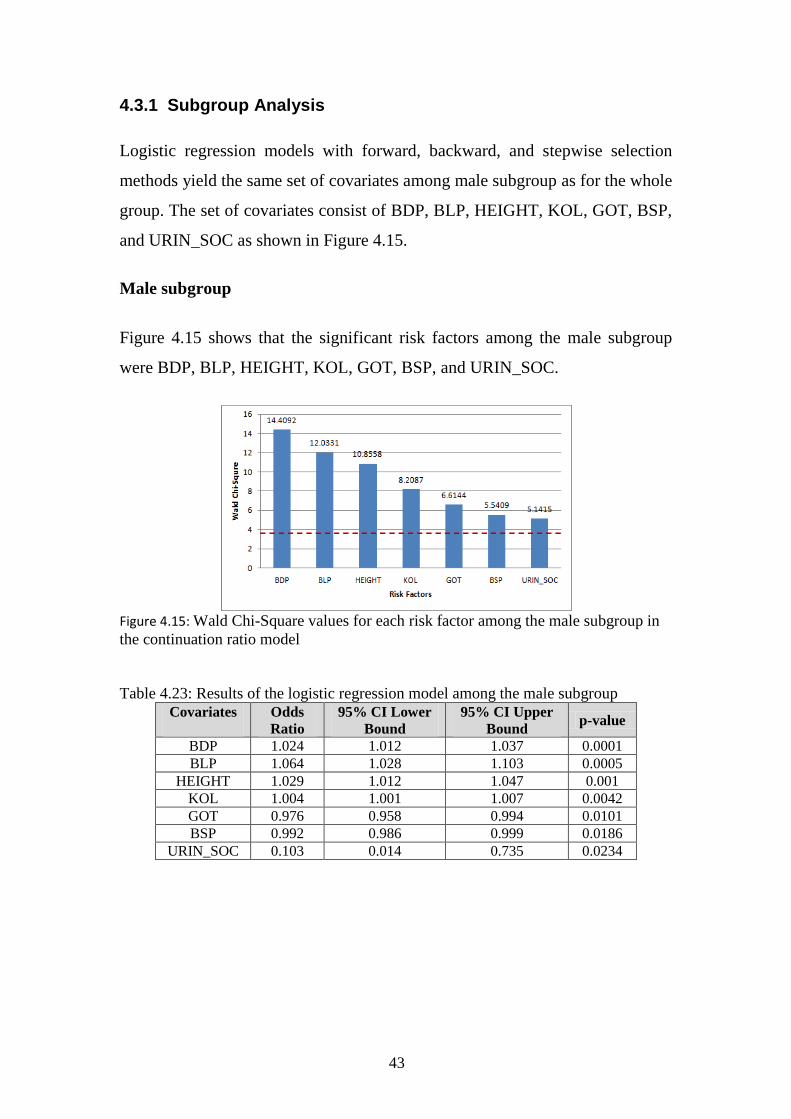
4.3.1 Subgroup Analysis
Logistic regression models with forward, backward, and stepwise selection
methods yield the same set of covariates among male subgroup as for the whole
group. The set of covariates consist of BDP, BLP, HEIGHT, KOL, GOT, BSP,
and URIN_SOC as shown in Figure 4.15.
Male subgroup
Figure 4.15 shows that the significant risk factors among the male subgroup
were BDP, BLP, HEIGHT, KOL, GOT, BSP, and URIN_SOC.
Figure 4.15: Wald Chi-Square values for each risk factor among the male subgroup in
the continuation ratio model
Table 4.23: Results of the logistic regression model among the male subgroup
Covariates
Odds
Ratio
95% CI Lower
Bound
95% CI Upper
Bound p-value
BDP 1.024 1.012 1.037 0.0001
BLP 1.064 1.028 1.103 0.0005
HEIGHT 1.029 1.012 1.047 0.001
KOL 1.004 1.001 1.007 0.0042
GOT 0.976 0.958 0.994 0.0101
BSP 0.992 0.986 0.999 0.0186
URIN_SOC 0.103 0.014 0.735 0.0234

44
Female subgroup
Figure 4.16: Wald Chi-Square values for each risk factor among the female subgroup
in the logistic regression model
Figure 4.16 presents that there were 4 risk factors among the female subgroup
which were KOL, BSP, BDP, and AGE.
Table 4.24: Results of the continuation ratio model among female subgroup
BDP, BSP, and KOL are significant in both the male and the female subgroup.
BLP, HEIGHT, GOT, and URIN_SOC are significant among the male
subgroup while AGE is only significant among the female subgroup.
Covariates Odds
Ratio
95% CI
Lower Bound
95% CI
Upper Bound p-value
KOL 1.008 1.004 1.012 <.0001
BSP 0.98 0.968 0.992 0.0013
BDP 1.033 1.01 1.056 0.0045
AGE 1.026 1.007 1.046 0.0082

45
Prediction Part
The dataset is divided into two parts: 70 percent for the training set and 30
percent for the test set. The training set consists of 44,690 participants (305
participants who experienced aortic aneurysm). The test set, consists of 19,154
participants (132 deaths from aortic aneurysm). Each method presents below
used the same set of covarites: AGE, SEX, BDP, BSP, KOL, BLP, SIA,
HEIGHT, URIN_SOC, and GOT. In order to compare the accuracy of the
methods, the results from test set are used.
4.4 The Cox Regression Model
Cox regression model is normally used to find the risk factors. However, Cox
regression can be applied for predicting the health outcome as well. The area
under ROC curve (AUC) obtains by the Cox regression with the test set is
0.6232. The ROC curve can be found in Figure A-1 in the Appendix.
4.5 The Continuation Ratio Model
Continuation ratio model is one of the alternative models to predict the health
outcome. With the continuation ratio model applied the AUC is 0.7257. The
ROC curve can be found in Figure A-2 in the Appendix.
4.6 The Logistic Regression Model
Logistic regression is once again applied in order to predict the response
variable. The result of the area under ROC curve is 0.7251. The ROC curve can
be found in Figure A-3 in the Appendix.
4.7 The Artificial Neural Network
The follow-up time is included as an additional covariate in the artificial neural
network. The output can be interpreted as the cumulative probability of relapse

46
for individual participants (Jerez et al., 2005). The Multilayer perceptron
network with the hyperbolic tangent activation function and different number
of hidden neurons is trained. Then, the areas under ROC curves are obtained.
Table 4.25: Results of different settings from neural network
Combination
function
Number of
hidden layer(s)
Number of
neurons AUC
Additive 1
1
1
1
3
4
5
6
0.6397
0.6397
0.6397
0.6397
Linear
1
1
1
1
3
4
5
6
0.5191
0.5776
0.5080
0.5758
Table 4.25 presents the area under ROC curves with the different settings. The
additive combination function performed better than linear combination
function in every settings. The AUCs from the additive combination function
are the same when the number of neurons is between 3 and 6 neurons.
Moreover, the best performance is obtained with 3 neurons, when the AUC is
0.6397. The ROC curve can find in Figure A-4 in the Appendix.
4.8 The Decision Tree
Decision tree analysis is performed by using CART method, which creates
binary splits on both interval and nominal covariate variables. The set of
covariates without the time of follow-up is used as input variables.
Table 4.26 shows that the decision tree with 30 splits search, 5 depths, and gini
reduction as splitting criterion performs the best. The AUC is 0.6793. The
ROC curve can be found in Figure A-5 in the Appendix.

47
Table 4.26: Results of different settings from decision tree
Splitting criterion Number of a split search Depth of tree AUC
Etropy reduction 20 25 30 35 25
5 5 5 5 6
0.6263 0.6620 0.5996 0.6615 0.6526
Gini reduction 15 20 25 30 35 20 30
5 5 5 5 5 6 6
0.6273 0.6561 0.6535 0.6793 0.5346 0.6479 0.6592
Figure 4.17: Decision tree graph
The first column in each box in Figure 4.17 represents the response values,
where ‘1’ means experiencing aortic aneurysm and ‘0’ means not experiencing
aortic aneurysm. The second and third columns stand for the percent and
number of participants in the training set and the test set, respectively. The
color denotes node purity: yellow color represent the impurity node.
48
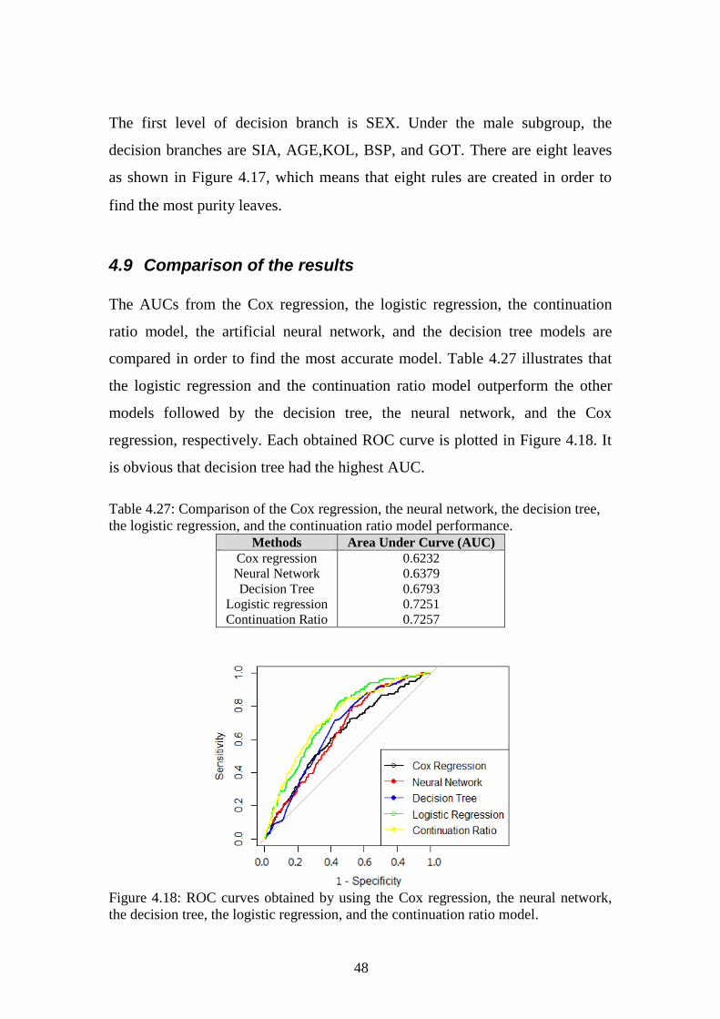
The first level of decision branch is SEX. Under the male subgroup, the
decision branches are SIA, AGE,KOL, BSP, and GOT. There are eight leaves
as shown in Figure 4.17, which means that eight rules are created in order to
find the most purity leaves.
4.9 Comparison of the results
The AUCs from the Cox regression, the logistic regression, the continuation
ratio model, the artificial neural network, and the decision tree models are
compared in order to find the most accurate model. Table 4.27 illustrates that
the logistic regression and the continuation ratio model outperform the other
models followed by the decision tree, the neural network, and the Cox
regression, respectively. Each obtained ROC curve is plotted in Figure 4.18. It
is obvious that decision tree had the highest AUC.
Table 4.27: Comparison of the Cox regression, the neural network, the decision tree,
the logistic regression, and the continuation ratio model performance.
Methods Area Under Curve (AUC)
Cox regression
Neural Network
Decision Tree
Logistic regression
Continuation Ratio
0.6232
0.6379
0.6793
0.7251
0.7257
Figure 4.18: ROC curves obtained by using the Cox regression, the neural network,
the decision tree, the logistic regression, and the continuation ratio model.

49
5 Discussion
5.1 Risk Factors for Aortic Aneurysm
SEX
SEX was found as the most important risk factor in all of the models (Cox
regression, continuation ratio, and logistic regression). Several studies also
reported that the male gender was a strong risk factor for experiencing aortic
aneurysm (Cornuz et al., 2004; Iribarren et al., 2007; Forsdahl et al., 2009).
Our study has found that the hazard of experiencing aortic aneurysm among
males is 3.824 times higher than females. Additionally, the KM estimator also
shows that the male subgroup has more risk of experiencing aortic aneurysm
than has the female subgroup.
AGE
AGE was the strongest significant covariate in the Cox regression model and
the continuation ratio model. Each additional year of AGE increased the hazard
by 1.2 percent. Our study supports what has been previously reported that there
is an association between older age and aortic aneurysm (Iribarren et al., 2007;
Forsdahl et al., 2009; Baguet et al., 2012). Moreover, AGE was found as a risk
factor in both male and female subgroups in the Cox regression.
Blood Diastolic Pressure (BDP)
Blood diastolic pressure (BDP) can indicate presence of the hypertension,
which is one of the risk factors for several diseases. Hypertension has
previously been claimed as a risk factor of aortic aneurysm (Iribarren et al.,
2007; Forsdahl et al., 2009; Baguet et al., 2012). From the Cox regression, it
was found that the hazard for the patients who had stage 1 of hypertension (90
– 99 mm/Hg) of having aortic aneurysm was 1.663 times higher than for the

50
normal BDP group. In the group of stage 2 of hypertension (≥100 mm/Hg), the
corresponding hazard ratio of experiencing aortic aneurysm was 1.69.
In all models (Cox regression, continuation ratio, and logistic regression), it
was shown that BDP was the most strongly significant covariate in the male
group but not strongly significant in the female group.
Beta-lipoprotein (BLP)
Beta-lipoprotein (BLP) is a rough measurement of LDL cholesterol and this
covariate is an alternative risk factor. Our study disclosed that BLP was a
significant risk factor in the main model and in the male subgroup. The survival
curve from Kaplan-Meier estimator indicated that an elevated level of BLP
increased the risk of experiencing aortic aneurysm.
Cholesterol (KOL)
Cholesterol (KOL) is associated with an increasing risk of aortic aneurysm
(Iribarren et al., 2007). In our study, KOL was significant in every model in our
study. It was found that an elevated level of KOL increased the risk of having
aortic aneurysm, especially at high level of KOL (≥240). Moreover, KOL and
BLP were strongly correlated.
HEIGHT
HEIGHT has previously been claimed as an alternative risk factor for aortic
aneurysm (Iribarren et al., 2007). HEIGHT was also one of the significant risk
factors in our study, but it was only significant in the main model and in the
male subgroup. For each additional unit (cm), the hazard increased by 2.1 and
0.9 percent in the main model and male subgroup, respectively.
Urinary glucose (URIN_ SOC)
Urinary glucose (URIN_SOC) is used as an indicator of diabetes. Several
previous studies also claimed that diabetes is a risk factor for aortic aneurysm

51
(Shantikumar et al., 2010). In our study, URIN_SOC was borderline significant
and URIN_SOC was only significant in the male subgroup.
Glutamic Oxalacetic Transaminase (GOT)
Glutamic Oxalacetic Transaminase (GOT) is usually found when the heart
muscle or liver is damaged. In our study, GOT was statistically significant in
the male subgroup and an increase in GOT was also linked with a decreased
risk of aortic aneurysm.
Sialic acid (SIA)
Sialic acid (SIA) is considered to be a marker for some diseases and it was a
statistically significant risk factor in Cox regression model. For each unit
(mg/dl) increased of SIA, the hazard increased by 1.9 percent.
5.2 Prediction
The goal of the study was to find the best performance model for prognosis.
Five models were developed: the Cox regression, the continuation ratio model,
the logistic regression, the neural network, and the decision tree. All of the risk
factors from the study on risk factors were used as input variables and having
or not having aortic aneurysm disease was used as a target variable.
In our study, accuracies of the five models were compared and the goal was to
find the model with the highest accuracy. The logistic regression and the
continuation ratio model had comparable performances with an AUC value of
0.7251 and 0.7257, respectively. Moreover, these two methods were found to
be the best model to predict the health outcome in our study. The decision tree
ranked the second accuracy (AUC = 0.6793) followed by the artificial neural
network (AUC = 0.6379), and the Cox regression (AUC = 0. 6232).

52
The artificial neural network model did not outperform the others, which was
surprising, since the artificial neural network has been shown to solve complex
problems such as survival data with high accuracy (Ohno-Machado, 1996). The
relations among different factors and the health outcome are usually non-linear
in nature and the artificial neural network is claimed to perform well in this
case. The reason why the artificial neural network did not produce a good
model here might be due to the low prevalence of the disease. If the relative
frequency of a certain characteristic in a population is below 1 percent, the
back-propagation neural network will have difficulties in identifying the rare
category (Ohno-Machado, 1996). The training set has only 0.68 percent of
participants who experienced aortic aneurysm; thus, the artificial neural
network may fail to recognize the pattern.

53
6 Conclusions
The first part of this study was to find the risk factors for aortic aneurysm. The
major findings were as follows:
Our results indicated that SEX was the most influential risk factor. Male
gender increased the hazard of experiencing aortic aneurysm 3.824 times in
comparison with female gender. Moreover, SEX was strongly and
moderately significant in the age group between 40 to 55 years old and in
the oldest age group (>65 years), respectively.
Blood diastolic pressure (BDP) was strongly significant in the main model.
Only the stage 1 of hypertension was significant in both the male and the
female subgroup while stage 2 of hypertension was only significance in the
male subgroup.
Beta-lipoprotein (BLP) was strongly significant in main model and the
male subgroup. The Kaiser-Meier estimator showed that an elevated level
of BLP (≥12 mg/dl) increased the risk of experiencing aortic aneurysm.
Cholesterol (KOL) was also found as one of the risk factors in the main
model and male subgroup. Elevated KOL (≥200mg/dl) may cause the
aortic aneurysm.
Glutamic Oxalacetic Transaminase (GOT) was moderately significant in
the main model and the male subgroup. Our study indicated that an
increase in GOT decreased the risk of experiencing aortic aneurysm.
Urinary glucose (URIN_SOC) was borderline significant in the main
model and this study thus indicated that it was found as a prevalence factor
in aortic aneurysm.
For the prediction part, the five methods (Cox regression, continuation ratio
model, logistic regression, artificial neural network, and decision tree) were
performed in order to predict aortic aneurysm. Our study found out that the
logistic regression model and the continuation ratio model showed the highest
AUCs or accuracy followed by the decision tree, the artificial neural network,
and the Cox regression.

54
7 Literature
Allison P. D. (1999) Logistic Regression Using the SAS® System: Theory and
Application. Cary, NC: SAS Institute Inc.
Allison P. D. (2010) Survival Analysis Using SAS®: A Practical Guide, Second
Edition. Cary, NC: SAS Institute Inc.
Armstrong B. G., & Sloan M. (1989). Ordinal regression models for epidemiologic
data. American Journal of Epidemiology, 129, 1, 191-204.
Baguet J.-P., Barone-Rochette G., Mallion J.-M., Chavanon O., Sessa C., Thony F., &
Lantelme P. (2012). European Society of Hypertension scientific newsletter:
Hypertension and aortic diseases. Journal of Hypertension, 30, 2, 440-443.
Bellazzi R, Zupan B. (2008). Predictive data mining in clinical medicine: current
issues and guidelines. Int J Med Inform, 77(2):81–97.
Berry, M. J. A., & Linoff, G. (2004). Data mining techniques: For marketing, sales,
and customer relationship management. Indianapolis, Ind: Wiley Pub.
Bewick Viv, Cheek Liz, & Ball Jonathan. (2004). Statistics review 13: Receiver
operating characteristic curves. (BioMed Central Ltd.) BioMed Central Ltd.
Cios KJ, Moore GW. (2002). Uniqueness of medical data mining. Artif Intell Med.
26:1–24. doi: 10.1016/S0933-3657(02)00049-0.
Collett D. (2003) Modeling Survival Data in Medical Research, Chapman & Hall,
New York.
Colombet I., Ruelland A., Chatellier G., Gueyffier F., Degoulet P., & Jaulent M. C.
(2000). Models to predict cardiovascular risk: comparison of CART, multilayer
perceptron and logistic regression. American Medical Informatics Association.
Cornuz J., Sidoti P. C., Tevaearai H., & Egger M. (2004). Risk factors for
asymptomatic abdominal aortic aneurysm: systematic review and meta-analysis of
population-based screening studies. European Journal of Public Health, 14, 4, 343-9.
Cox D. R. (1972). Regression models and life-tables (with discussion). Journal of the
Royal Statistical Society, Series B, 34, 187-220.
Forsdahl S.H., Singh K., Solberg S., Jacobsen B.K. (2009). Risk factors for abdominal
aortic aneurysms: a 7-year prospective study: the tromso study, 1994–2001.
Circulation. 119(16):2202–2208.
GÖnen, Mithat. (2007). Analyzing Receiver Operating Characteristic Curves with
SAS®. Cary. NC: SAS Institute Inc.
Harrell F.E. Jr., Margolis P.A., Gove S., Mason K.E., Mulholland E.K., Lehmann D.
et al. (1998). Development of a clinical prediction model for an ordinal outcome: the
World Health Organization Multicentre Study of Clinical Signs and Etiological agents

55
of Pneumonia, Sepsis and Meningitis in Young Infants. WHO/ARI Young Infant
Multicentre Study Group. Stat Med. 17(8):909–44.
Hosmer D. W. & Lemeshow S. (1999) Applied Survival Analysis, John Wiley & Sons,
New York.
Hosmer, D. W., & Lemeshow, S. (2000) Applied logistic regression. New York:
Wiley.
Hultgren, R., Forsberg, J., Alfredsson, L., Swedenborg, J., & Leander, K. (2012).
Regional variation in the incidence of abdominal aortic aneurysm in Sweden. The
British Journal of Surgery, 99, 5, 647-53.
Iribarren C., Darbinian J. A., Go A. S., Fireman B. H., Lee C. D., Grey, D. P. (2007).
Traditional and Novel Risk Factors for Clinically Diagnosed Abdominal Aoritc
Aneurysm: The Kaiser Multiphasic Heath Checkup Cohort Study. Ann EpidemiolI. 17
(9): 669-78
Jerez J. M., Franco, L., Alba, E., Llombart-Cussac, A., Lluch, A., Ribelles, .,
Mun arri , B., Mart in, M. (2005). Improvement of breast cancer relapse prediction
in high risk intervals using artificial neural networks. Breast Cancer Research and
Treatment, 94, 3, 265-272.
Kirkwood B. R., Sterne J. A. C., & Kirkwood, B. R. (2003). Essential medical
statistics. Malden, Mass: Blackwell Science.
Matignon R., & SAS Institute. (2007). Data mining using SAS Enterprise miner.
Hoboken, N.J: Wiley-Interscience.
McCullagh P. (1980) Regression models for ordinal data (with discussion). Journal of
the Royal Statistical Society – B 42, 109-142.
O'Connell A.A. (2006). Logistic Regression Models for Ordinal Response Variables.
Quantitative Applications in the Social Sciences. Thousand Oaks, CA: Sage
Publications.
Ohno-Machado L. (1996). Medical Applications of Artificial Neural Networks:
Connectionist Models of Survival. (Doctoral dissertation). Retrieved from ProQuest
Dissertations and Theses.
Ozkan C., & Erbek F. S. (2003). A Comparison of Activation Functions for
Multispectral Landsat TM Image Classification - The main objective of the study was
to compare linear, sigmoid, and tangent hyperbolic activation functions through the
one- and two-hidden layered MLP neural network structures trained with the scaled
conjugate gradient learning algorithm, and to evaluate their performances for a
multispectral Landsat TM imagery hard classification problem. Photogrammetric
Engineering and Remote Sensing, 69, 11, 1225.
56
Pampel F. C. (2000). Logistic regression: A primer. Thousand Oaks, Calif: Sage
Publications.
Shantikumar S, Ajjan R, Porter KE, (2010). Diabetes and the abdominal aortic
aneurysm. Eur J Vasc Endovasc Surg. 39(2):200–7.
Singer J. D. & Willett, J. B. (2003) Applied Longitudinal Data Analysis: Modeling
Change and Event to Occurrence. New York: Oxford University Press.
Törnberg S. A., Carstensen J. M., Holm L. E. (1988). Risk of stomach cancer in
association with serum cholesterol and beta-lipoprotein. Acta Oncol. 27:39–42.
Podgorelec V, Kokol P, Stiglic B, Rozman I. (2002). Decision trees: an overview and
their use in medicine. J Med Syst. 26:445–463. doi: 10.1023/A:1016409317640.
Zweig M. H., & Campbell G. (1993). Receiver-operating characteristic (ROC) plots: a
fundamental evaluation tool in clinical medicine. Clinical Chemistry, 39, 4, 561-77.

57
8 Appendix
Figure A-1: The ROC curve obtained by using the Cox regression
Figure A-2: The ROC curve obtained by using the continuation ratio model

58
Figure A-3: The ROC curve obtained by using the logistic regression
Figure A-4: The ROC curve obtained by using the decision tree

59
Figure A-5: The ROC curve obtained by using the neural network

60
LIU-IDA/STAT-A--12/005--SE