Embed Size (px)
Citation preview

Faculty of Science and Technology
MASTER’S THESIS
Study program/ Specialization:
Master of Science in Petroleum Engineering,
Drilling and Well Technology.
Spring semester, 2012
Open
Writer:
Kanokwan Kullawan
………………………………………… (Writer’s signature)
Faculty supervisor: Kjell Kåre Fjelde, University of Stavanger
External supervisor(s):
Titel of thesis:
Risk Based Cost and Duration Estimation of Well Operations.
Credits (ECTS): 30
Key words: Drilling Cost Estimation, Well
Cost Estimation, Probabilistic Cost
Estimation, AFE Writing, Cost and Duration
Estimation, Risk Analysis.
Pages: 113
+ enclosure: 2
Stavanger, 04-June-2011
Date/year

Risk Based Cost and Duration Estimation of Well Operations 2012
Kanokwan Kullawan
1
Abstract
Due to high uncertainties and the cost intensive nature of well operations, accurate forecast of
well cost and duration is one of the main requirements for writing an AFE and supporting
decision making processes. Traditionally, the well cost has been estimated by the
deterministic approach. However, this method has some limitations and the actual operating
costs can significantly exceed the planned budget. Thus, the probabilistic approach of well
cost estimation along with risk assessment has been developed and considered a more
appropriate approach for dealing with well cost estimation.
There are many simulation tools which are available in the market. Nevertheless, the Risk€
software, developed by IRIS, is the simulation tool used here. This software also provides the
function of including undesirable events into the simulation. Thus, risks associated with the
well operations can be assessed effectively.
An example well model is created and the characteristics of the results are studied. Detailed
analysis has been performed to observe how the changes in input parameters can affect the
uncertainties and values of the simulated results. The case construction was inspired by a
drilling program that was released from Statoil through the Academia program for teaching
purpose.
The simulation showed that drilling and mobilization phases have the largest influence on the
total well cost and duration. Besides, detailed sensitivity analysis revealed that better
information of an expected range of ROP can greatly reduce the uncertainties of the results.
When the expected values are analysed, the results demonstrate asymmetric behaviour. The
effect on total duration and cost when the operation is slower is much greater than when it is
faster.
Risk events are included in the simulation with an assumption that the problems can be
solved and there is no extra cost associated with the events, only extra duration. Comparison
between the standard operation plan and the risk operation plan also shows that unwanted
events can drastically increase the uncertainties of the results and failure to include risk
events in the forecast can lead to improper budget assigned to the project.
For future study, the software should be developed to handle more well operations scenario;
such as multilateral well, lost in hole (LIH) situation, batch drilling including the effect of

Risk Based Cost and Duration Estimation of Well Operations 2012
Kanokwan Kullawan
2
learning curve and the completion phases. The software could also be extended for analysing
new drilling technologies. Thus, well cost and duration estimation in various situations can be
performed.

Risk Based Cost and Duration Estimation of Well Operations 2012
Kanokwan Kullawan
3
Acknowledgement
This thesis would have remained a dream without the help and support from many wonderful
people around me, only some of those whom it is possible to give a particular mention here.
First and foremost, I would like to thank my professor, Kjell Kåre Fjelde, for his supervision,
advice and guidance throughout this thesis. I would like to express my immense gratitude for
giving me academic insights and encouragement during this study.
My grateful thanks also go to IRIS, especially Øystein Arild, for providing me with the
software to use in this thesis and Talisman Energy for offering the scholarship and summer
internship during my master study in Norway.
I owe my deepest gratitude to my parents, Amphol and Pongthip, and my family for giving
birth to me, providing me with the best educations and giving me support throughout my life.
Above all, I would like to dedicate this thesis to my aunt, Malai Kullawan, to whom I cannot
find words to express my gratitude. I extremely thankful that she has always stood by me,
believed in me, and given me unequivocal support and patience such that my mere
expressions of thanks would not have been sufficient.
Last, but not least, special thanks go to all the professors and staffs in the department of
petroleum engineering, University of Stavanger and my friends in Thailand, Norway and
elsewhere for their help, support and encouragement in every way.
For any inadequacies and errors that may remain in this study, the responsibility is entirely
my own.
Kanokwan Kullawan

Risk Based Cost and Duration Estimation of Well Operations 2012
Kanokwan Kullawan
4
Table of Contents
Abstract ...................................................................................................................................... 1
Acknowledgement ..................................................................................................................... 3
List of Figures ............................................................................................................................ 8
List of Tables ........................................................................................................................... 10
Nomenclature ........................................................................................................................... 11
1. Introduction .......................................................................................................................... 12
1.1 Background .................................................................................................................... 12
1.2 Challenges Related to Well Cost Estimation ................................................................. 13
1.3 Study Objectives ............................................................................................................ 14
1.4 Structure of the Thesis ................................................................................................... 15
2. Well Cost Estimation ........................................................................................................... 16
2.1 AFE Writing Procedures ................................................................................................ 16
2.2 Deterministic Well Cost Estimation .............................................................................. 17
2.2.1 Advantages of the Deterministic Approach ............................................................ 17
2.2.2 Limitations of the Deterministic Approach ............................................................ 17
2.3 Probabilistic Well Cost Estimation ................................................................................ 19
2.3.1 Advantages of the Probabilistic Approach ............................................................. 19
2.3.2 Limitations of the Probabilistic Approach .............................................................. 20
2.4 Software Available in the Market .................................................................................. 21
2.4.1 Commercial Software ............................................................................................. 21
2.4.2 Company Developed Software ............................................................................... 22
2.4.3 Software Product from Service Companies ............................................................ 22
2.5 Development of Probabilistic Approach and Monte Carlo Simulation in Well Cost
Estimation ............................................................................................................................ 23
2.6 Statistics Refresher......................................................................................................... 26
Risk Based Cost and Duration Estimation of Well Operations 2012
Kanokwan Kullawan
5
2.7 Probability Distribution ................................................................................................. 27
2.7.1 Uniform Distribution .............................................................................................. 27
2.7.2 Triangular Distribution ........................................................................................... 28
2.7.3 Normal Distribution ................................................................................................ 29
2.7.4 Lognormal Distribution .......................................................................................... 30
2.7.5 Weibull Distribution ............................................................................................... 30
2.7.6 Discrete Distribution ............................................................................................... 31
2.7.7 Examples of Variables Represented by Each Type of Probability Distribution ..... 32
3. Monte Carlo Simulation ....................................................................................................... 33
3.1 Procedure of Monte Carlo Simulation ........................................................................... 33
3.1.1 Define an Appropriate Model ................................................................................. 33
3.1.2 Data Gathering ........................................................................................................ 34
3.1.3 Select Suitable Probability Distribution for Input Variables .................................. 34
3.1.4 Randomly Sample Input Distributions.................................................................... 34
3.1.5 Compute the Model Results and Generate Statistics of Results ............................. 36
3.2 Advantages of Monte Carlo Simulation ........................................................................ 37
3.3 Common Pitfalls in Performing Monte Carlo Simulation ............................................. 38
3.4 Dependencies ................................................................................................................. 40
3.5 Example Calculation using Monte Carlo Simulation .................................................... 41
3.6 Sensitivity Analysis ....................................................................................................... 45
4. Major Risk Events that Cause Delay in Well Operations .................................................... 47
4.1 Kick ................................................................................................................................ 47
4.1.1 Causes of Kick Incidents ........................................................................................ 48
4.2 Stuck pipe....................................................................................................................... 49
4.2.1 Causes of Stuck Pipe Incidents. .............................................................................. 49
4.3 Wait on Weather (WOW) or other environmental interruptions ................................... 51
4.4 Downhole tool failure .................................................................................................... 52

Risk Based Cost and Duration Estimation of Well Operations 2012
Kanokwan Kullawan
6
4.5 Lost Circulation ............................................................................................................. 53
4.6 Shallow gas .................................................................................................................... 54
5. Simulation Tool ................................................................................................................... 55
5.1 Benefits of Risk€ Software ............................................................................................ 55
5.2 Applications ................................................................................................................... 56
5.3 Input of Drilling Phases for Generation of Standard Operation Plan ............................ 57
5.3.1 Well Architecture .................................................................................................... 58
5.3.2 Mobilization of drilling rig ..................................................................................... 58
5.3.3 Spudding ................................................................................................................. 60
5.3.4 Drilling hole sections .............................................................................................. 61
5.3.5 BOP Editor .............................................................................................................. 62
5.3.6 Distribution Mode Input ......................................................................................... 63
5.4 Input of Risk Events for Generation of Risk Operation Plan ........................................ 64
5.4.1 Risk Events in Well Level ...................................................................................... 64
5.4.2 Risk Events in Phase Level ..................................................................................... 65
5.5 Simulation Results ......................................................................................................... 70
6. Simulations and Discussions of an Example Well using Risk€ .......................................... 73
6.1 Background .................................................................................................................... 73
6.2 Input Data....................................................................................................................... 77
6.3 Results from Standard Operation Plan ........................................................................... 79
6.3.1 Deterministic View ................................................................................................. 79
6.3.2 Probabilistic View ................................................................................................... 80
6.4 Detailed Sensitivity Analysis ......................................................................................... 84
6.4.1 Detailed Analysis of ROP ....................................................................................... 84
6.4.2 Detailed Analysis of Rig Mobilization Velocity .................................................... 89
6.5 Results from Risked Operation Plan .............................................................................. 94
6.5.1 Input of Risk Events into the Well Model .............................................................. 94

Risk Based Cost and Duration Estimation of Well Operations 2012
Kanokwan Kullawan
7
6.5.2 Results of Risked Operation Plan ........................................................................... 96
6.5.3 Comparison of Results between Standard Operation Plan and Risk Operation Plan
.......................................................................................................................................... 97
6.5.4 Detailed Sensitivity Analysis of Undesirable Events ............................................. 98
7. Conclusions and Recommendations .................................................................................. 105
7.1 Why Probabilistic Cost Estimation .............................................................................. 105
7.2 Conclusions from an Example Well ............................................................................ 106
7.3 Recommendations for Future Study and Software Development................................ 108
7.3.1 Software Development to Cover More Well Operations Situations ..................... 108
7.3.2 Software Development to Enhance Efficiency in Simulation Process ................. 109
References .............................................................................................................................. 111
Appendix A: Matlab Code ..................................................................................................... 114

Risk Based Cost and Duration Estimation of Well Operations 2012
Kanokwan Kullawan
8
List of Figures
Figure 1: Time – Depth Curve and Time - Cost Curve given by a deterministic cost and time
estimation (Figure taken from Risk€ Software)....................................................................... 18
Figure 2: Uniform distribution plot.......................................................................................... 28
Figure 3: Triangle distribution plot. ......................................................................................... 28
Figure 4: Normal distribution plot. .......................................................................................... 29
Figure 5: Lognormal distribution shape. .................................................................................. 30
Figure 6: Weibull Distribution with scale parameter = 1 - Source: [4] ................................... 31
Figure 7: Weibull Distribution with shape parameter = 3 – Source: [4] ................................. 31
Figure 8: Discrete Distribution plot. ........................................................................................ 31
Figure 9: Schematic of input parameter generation. – Source: [6] .......................................... 35
Figure 10: Schematic of Monte Carlo simulation procedure – Source:[6] .............................. 36
Figure 11: Linear correlation - Source: [6] .............................................................................. 40
Figure 12: Histogram of ROP with normal distribution .......................................................... 41
Figure 13: Histogram of rig rental rate with uniform distribution ........................................... 42
Figure 14: Histogram of estimated drilling cost ...................................................................... 42
Figure 15: Histogram of estimated drilling cost with the risk of events included ................... 43
Figure 16: Cost sensitivity analysis. - Source: [7] ................................................................... 46
Figure 17: Kick illustration – KICK occurring. - Source:[5]................................................... 47
Figure 18: Kick illustration – drill bit hit high - Source:[5] .................................................... 47
Figure 19: Mobile formation causes stuck pipe incident – Source: [2] ................................... 50
Figure 20: Lost circulation - source:[1] ................................................................................... 53
Figure 21: Snapshot of operation plan automatically created in RiskE ................................... 57
Figure 22: Input panel for well architecture ............................................................................ 58
Figure 23: Mobilization phase input panel. ............................................................................. 60
Figure 24: Spudding Phase Input Panel ................................................................................... 61
Figure 25: Drilling phase input panel ...................................................................................... 62
Figure 26: BOP editor input panel ........................................................................................... 63
Figure 27: Distribution Mode Input Panel ............................................................................... 63
Figure 28: Input panel for risk events in well level ................................................................. 65
Figure 29: Input panel for risk events in phase level ............................................................... 68

Risk Based Cost and Duration Estimation of Well Operations 2012
Kanokwan Kullawan
9
Figure 30: Snapshot of risk operation plan .............................................................................. 69
Figure 31: Well summary result .............................................................................................. 70
Figure 32: Result view of phase sensitivity ............................................................................. 71
Figure 33: Result of operation sensitivity ................................................................................ 71
Figure 34: Result view of cost breakdown .............................................................................. 72
Figure 35: Wellbore schematic of pilot hole............................................................................ 74
Figure 36: Deterministic view from the result of the standard operation plan ........................ 79
Figure 37: Well summary result from standard operation plan ............................................... 80
Figure 38: Phase sensitivity from standard operatoin plan ...................................................... 81
Figure 39: Operation sensitivity from standard operation plan ............................................... 82
Figure 40: Cost Breakdown of standard operation plan .......................................................... 83
Figure 41: Uncertainties in well duration for different ROP distribution ................................ 85
Figure 42: Uncertainties in well cost for different ROP distribution....................................... 86
Figure 43: Expected well duration for different ROP value .................................................... 87
Figure 44: Expected well cost for different ROP value ........................................................... 88
Figure 45: Summary of typical drilling rig time distribution – Source: [3] ............................. 89
Figure 46: Uncertainties in well duration for different rig velocity distribution type ............. 90
Figure 47: Uncertainties in well cost for different rig velocity distribution type .................... 91
Figure 48: Expected well duration for different rig velocity ................................................... 92
Figure 49: Expected well cost for different rig velocities ........................................................ 93
Figure 50: Well summary results of risked operatoin plan ...................................................... 96
Figure 51: Events sensitivity analysis ...................................................................................... 96
Figure 52: Results comparison between standard operation plan and risk operation plan ...... 97
Figure 53: Result of risk operation plan without WOW event ................................................ 98
Figure 54: Result of risk operation plan without kick event ................................................... 98
Figure 55: Result of risk operation plan without BHA failure event ....................................... 99
Figure 56: Result of risk operation plan without stuck pipe event .......................................... 99
Figure 57: Uncertainties in well duration for different operation plan .................................. 100
Figure 58: Uncertainties in well cost for different operation plan ......................................... 101
Figure 59: Uncertainties in well duration for different probability of WOW event .............. 102
Figure 60: Uncertainties in well cost for different probability of WOW event ..................... 102
Figure 61: Expected well duration for different operation plan ............................................ 103
Figure 62: Expected well cost for different operation plan ................................................... 104

Risk Based Cost and Duration Estimation of Well Operations 2012
Kanokwan Kullawan
10
List of Tables
Table 1: Examples of variables represented by each type of probability distribution – Source:
[29],[10] ................................................................................................................................... 32
Table 2: Mobilize rig technology and its input information – Source:[42] ............................. 59
Table 3: Spudding technology and its input variables ............................................................. 60
Table 4: Well general information ........................................................................................... 73
Table 5: Section details ............................................................................................................ 74
Table 6: Summary of input parameters .................................................................................... 78
Table 7: Results comparison between deterministic and probabilistic approach .................... 80
Table 8: ROP input values for each distribution type. ............................................................. 85
Table 9: Well duration SD for each ROP distribution type ..................................................... 85
Table 10: Well cost SD for each ROP distribution type .......................................................... 86
Table 11: ROP inputs for value analysis.................................................................................. 87
Table 12: Expected duration from different ROP value .......................................................... 87
Table 13: Expected well cost from different ROP Value ........................................................ 88
Table 14: Rig moving velocity inputs for each distribution type ............................................ 89
Table 15: Well duration SD for each velocity distribution type .............................................. 90
Table 16: Well cost SD for each velocity distribution type ..................................................... 90
Table 17: Expected duration for each rig velocity ................................................................... 91
Table 18: Expected cost for each rig velocity .......................................................................... 92
Table 19: Input parameters for risk events .............................................................................. 95
Table 20: Comparison of standard operation plan and risk operation plan ............................. 97
Table 21: Well duration SD for different operation plan ......................................................... 99
Table 22: Well cost SD for different operation plan .............................................................. 100
Table 23: Expected duration for different operation plan ...................................................... 103
Table 24: Expected Cost for different operation plan ............................................................ 104

Risk Based Cost and Duration Estimation of Well Operations 2012
Kanokwan Kullawan
11
Nomenclature
AFE - Authorization For Expenditure
BHA - Bottom Hole Assemblies
BOP - Blow Out Preventer
CDF - Cumulative Distribution Function
HSE - Health, Safety and Environment
ID - Inner Diameter
LIH - Lost In Hole
LOT - Leak Off Test
LWD - Logging While Drilling
MCS - Monte Carlo Simulation
MD - Measured Depth
MU BHA - Make Up BHA
MWD - Measurement While Drilling
NOK - Norwegian Kroner
NPT - Non ProductiveTime
OAT - One At A Time
OD - Outer Diameter
OWC - Oil Water Contact
PDF - Probability Density Function
POOH - Pull Out Of Hole
RIH - Run In Hole
ROP - Rate Of Penetration
ROV - Remotely Operated Underwater Vehicle
RT - Rotary Table
SA - Sensitivity Analysis
SD - Standard Deviation
ST - Sidetrack
TD - Total Depth
TFT - Trouble-Free Time
UA - Uncertainty Analysis
USD - US Dollar
WOB - Weight On Bit
WOW - Wait On Weather

Risk Based Cost and Duration Estimation of Well Operations 2012
Kanokwan Kullawan
12
1. Introduction
1.1 Background
Among all petroleum exploration activities, drilling oil wells could be considered one of the
riskiest and most expensive ventures. Record high oil price and shortage supply on drilling
rigs, especially deep-water drilling rigs, have boosted the rig daily rental rate drastically over
the past decade. Due to that reason, one of the objectives in drilling a hydrocarbon well is too
make a hole in the ground as quickly as possible. However, there are 3 basic considerations
which are required for successful drilling operations. First of all, the well needs to be drilled
in a safe manner. Health, safety and environments, HSE, are always the top priorities
although it may lead to delay in operation or extra cost. Second, the well must fulfil the
requirements for its purpose either as an exploration, prospect appraisal or field development
well. Regardless of the well type, there are minimum demands for all the wells. They should
be drilled without damaging the borehole and the potential formations. They should also
allow for formation testing, data gathering, hydrocarbon production, or other post-drill
activity. The third basic consideration is that the overall well cost should be minimized. This
topic has been the point of interest for the industry for a long time. Several oil companies
have put a great effort in improving drilling efficiency and reducing drilling time in order to
lessen the overall well cost.[8]
Previously, success of drilling project was defined by the completion of the well construction
activities within the constraints of time, cost and performance. Nowadays, that definition has
been modified. In 2002, Harold Kerzner pointed out the key issues for the drilling projects
completion as shown below:[9]
- Within the allocated time period
- Within the budgeted cost
- At the proper performance or specification level
- Being accepted by the customer
- Without disturbing the main work flow of the organization
It is obvious that both cost and duration have always been considered as the key issues in
drilling business. Thus, accurate forecast for drilling time and cost is necessary for drilling
performance management.

Risk Based Cost and Duration Estimation of Well Operations 2012
Kanokwan Kullawan
13
1.2 Challenges Related to Well Cost Estimation
Although the companies are seeking for the correct estimate of well construction cost and
duration, to achieve that may not be straightforward as it seems. Some of the major
challenges related to well cost estimation are listed below:
One main source of information for the model input is the historical data. Despite of
that, there could be a shortcomings of the data acquired or the collected data may not
have sufficient level of details. Furthermore, the available data may not be relevant to
the wells being predicted.
Well construction processes are associated with risks of undesirable events. These
events, such as WOW, kick event, etc.; can cause delays in well operations. The total
operation time is the summation of the trouble-free time (TFT) and the non-
productive time (NPT). We may define TFT as the time required for planned
operation and NPT is the time that any unplanned operations consume.[10]
The challenge in writing AFE is that an extra duration caused by NPT could lead to a
risk of exceeding a planned budget. Thus, accurate forecast for well cost is important
so that appropriate budget is planned for drilling the well. There should be neither
lacking of funding situation nor unspent funds left.[11]
Besides the unwanted events, the planned operations are subjected to many
uncertainties due to both geological and technical factors. The processes may take
longer time than expected. This is where the probabilistic approach plays a significant
role.
Risk Based Cost and Duration Estimation of Well Operations 2012
Kanokwan Kullawan
14
1.3 Study Objectives
The main objectives of this thesis are to discuss different approaches for well cost estimation
as well as their advantages and limitations along with their development over time and to
combine major drilling risks into cost estimation. Besides, this study also aims at studying the
characteristics of the forecasted results and providing recommendations for the software
future development.

Risk Based Cost and Duration Estimation of Well Operations 2012
Kanokwan Kullawan
15
1.4 Structure of the Thesis
This thesis is divided into 7 chapters. The first chapter is the introduction part of this thesis
which covers the background of this study, what have made this topic challenging, the
objectives of this thesis and the structure of the thesis. In the second chapter, literature
reviews regarding well cost estimation have been performed. This chapter presents various
methods of performing well cost estimation, the software which is available in the market, its
development overtime and some statistical refresher. Chapter 3 discusses about the Monte
Carlo simulation and shows a calculation example using this technique. After that, some
major risk events which are associated with the drilling operations are explained in chapter 4.
Then, chapter 5 describes the Risk€ software which is the simulation tool used in this study.
Next, in chapter 6, the simulation of an example well has been conducted and the results are
discussed. Finally, the last chapter offers the conclusion of this study and the
recommendations for future study and the software development.

Risk Based Cost and Duration Estimation of Well Operations 2012
Kanokwan Kullawan
16
2. Well Cost Estimation
2.1 AFE Writing Procedures
“AFE (Authorization for Expenditure) is a budgetary document, usually prepared by the
operator, to list estimated expenses of drilling a well to a specified depth, casing point or
geological objective, and then either completing or abandoning the well. Such expenses may
include excavation and surface site preparation, the daily rental rate of a drilling rig, costs of
fuel, drillpipe, bits, casing, cement and logging, and coring and testing of the well, among
others. This estimate of expenses is provided to partners for approval prior to commencement
of drilling or subsequent operations. Failure to approve an authority for expenditure (AFE)
may result in delay or cancellation of the proposed drilling project or subsequent operation.
In short, it is the cost of drilling and constructing a well.”[12]
Generally, estimation of the well construction cost has been based on historical data. Major
operators collect a variety of data related to drilling operations, such as: [13],[14]
Time and cost information for various operations
Drilling problems, time and cost associated with the problems, and their solutions
Comparisons of drilling performance
Drilling engineers combine the offset wells data, engineering calculations, projections about
operational improvements and plan for contingency cost in order to write the AFE. These
data will be analysed for an estimation of drilling performance and the likelihood of facing
drilling problems. Expert judgments could also be added.
Due to extremely high cost of the daily rental rate of drilling rigs, the time taken to drill a
well could represent 70 to 80% of the final well cost. Since the duration of the well
construction has a significant impact on the budget planning, it becomes a common practice
to assess the well duration together with the well cost. There are two main approaches which
are commonly used for well cost estimation. These are the deterministic and the probabilistic
approach. More details about each method are described below.

Risk Based Cost and Duration Estimation of Well Operations 2012
Kanokwan Kullawan
17
2.2 Deterministic Well Cost Estimation
Traditionally, the well cost estimates have been developed by a deterministic approach. The
budget for the well construction cost has been based on a single value, a base-case cost. In
order to take uncertainties and risks into account, the optimistic case and the pessimistic case
could also be developed by adding or subtracting a certain percentage from the base-case
cost. The optimistic and pessimistic cases are sometimes mentioned as low and high cost
estimates. [7],[15]
2.2.1 Advantages of the Deterministic Approach
The deterministic approach is simple.
It has a clear set of assumptions.
The method gives quick results which are easy to communicate.
2.2.2 Limitations of the Deterministic Approach
From historical well cost estimates, the deterministic approach has been too optimistic.
The prediction may be subjected to technical imperfection such as systematic
underestimation.[16]
It does not reflect the full range of possible outcomes.
The likelihood of any particular outcomes and the probability that the actual well cost
will be the same or close to the predicted value are not quantified.
The figure below shows the results from a deterministic estimation of the well cost and
duration. The blue line is a time – depth curve which represents the relationship between the
progress of the well depth and the time spent on the processes. The red line is a time – cost
curve which illustrates the how the costs increase as the well operations are going on.

Risk Based Cost and Duration Estimation of Well Operations 2012
Kanokwan Kullawan
18
Figure 1: Time – Depth Curve and Time - Cost Curve given by a
deterministic cost and time estimation (Figure taken from Risk€ Software)

Risk Based Cost and Duration Estimation of Well Operations 2012
Kanokwan Kullawan
19
2.3 Probabilistic Well Cost Estimation
By the nature of oil & gas upstream operations, there are a lot of risks and uncertainties
associated with the activities. With the limitations of the deterministic method mentioned
before, the probabilistic method, also referred to as the stochastic method, is considered a
more suitable approach for dealing with uncertainties in time and cost management. This
method has quickly become a common business practice in the well construction industry.[17]
This concept also utilizes historical data from offset wells, but in the form of probability
distributions. Probabilistic technique provides many advantages for both users and decision
makers for maximizing correct decision making and preventing time and cost overrun.
The main concept of the probabilistic well construction time and cost estimation is to apply
the Monte Carlo simulation technique in combination with the use of probability distributions
for cost and duration estimation.
In addition, the probabilistic approach can include unwanted events into the well model,
which cannot be done by the deterministic approach. As a result, risk assessment can be
conducted more efficiently.
2.3.1 Advantages of the Probabilistic Approach
As the probabilistic approach is referred to as the more appropriate method for well cost
estimation, some of its advantages are listed below. [7],[17]
In probabilistic estimating, the stakeholders are better acknowledged with the
uncertainties in well construction operation and the range of expected outcome.
Risks and opportunities can be addressed earlier in the planning processes and the
awareness of risks, opportunities and their impact is significantly improved.
It helps the decision makers to make better decisions by using consistent methodology
in decision making process.
The offset data is analysed thoroughly which leads to better transfer in experiences and
best practices among the project teams.
This method allows for sensitivity analysis. Thus, more effective allocation of funding
and resources can be focused on the key cost drivers.
In the probabilistic approach, the well construction is broken down into consecutive
steps and the offset data is analysed along with the well model. This can clarify

Risk Based Cost and Duration Estimation of Well Operations 2012
Kanokwan Kullawan
20
opportunities and risks in performance. Thus, it supports the performance improvement
as well as pointing out the limitations of the technical process.
If there are several alternatives for the well construction process, comparison of the
alternatives can be provided.
It helps in cost-benefit evaluation of risk reducing measures. Planned well construction
is compared to an adjusted operation plan. The benefits of the adjusted plan can be
examined and balanced with the cost that needs to be spent on it.
It also promotes accurate recording and reporting of actual operation time and cost data,
which is important for performance management and improvement. Realizing that the
database is utilized significantly, the data collectors will have better understanding about
the necessity of good data quality.
It can identify the probability of finishing the well construction within a given time
window. This issue could be critical in some areas, e.g. in the Barents Sea, where the
drilling time window is tight. This is due to the fact that, in the Barents Sea, drilling is
only performed during the winter season for sea life protection.
2.3.2 Limitations of the Probabilistic Approach
Although the probabilistic approach brings many benefits and advantages which lead to
improvement in the planning and decision making process, the probabilistic assessment has
its limitations just as the deterministic approach. [17]
The probabilistic approach should never be expected to identify and capture all risks and
uncertainties. There will always be unknown unknowns.
The results from the analysis should always be accompanied with the philosophy used
in model construction. The users of the prediction results should understand the
assumptions used in the model.

Risk Based Cost and Duration Estimation of Well Operations 2012
Kanokwan Kullawan
21
2.4 Software Available in the Market
While performing probabilistic well cost estimation and/or Monte Carlo simulation, a number
of software can be used as a tool. Software selection varies with users and organizations.
Some companies have developed their own software or spreadsheet for drilling cost
forecasting purpose. Some organizations utilize available commercial software for their
prediction. Frequently, the commercial software used in cost estimation activity is a
spreadsheet-based application which allows users to perform Monte Carlo simulation from
their existing spreadsheet software. Major oil field service companies also offer well cost
estimation and risk analysis software as one of their services. In this case, the software
providers generally offer other services and/or software which have the potential to enhance
the efficiency of cost estimation.
Beside Risk€[18]
software which will be used in this thesis, examples of the software available
in the market will be described here.
2.4.1 Commercial Software
@Risk from Palisade Corporation[19]
: @Risk is an add-in to Microsoft Excel. This
software performs risk analysis using Monte Carlo simulation. The range of possible
outcomes and the likelihood that each result will occur are shown in Microsoft Excel
spreadsheet. This can help decision makers to make decisions under uncertainties. The
software has been used in various industries, from the financial to the scientific. In oil
and gas industry, its application is including, but not limited to, exploration and
production, oil reserves estimation, capital project estimation, pricing, and regulation
compliance.
When setting up the model, the user can select the probability distribution or define
the distribution from the historical data for a given input. The results from the
simulation are the whole range of possible outcomes with the probabilities they will
occur. It also offers the tornado chart and sensitivity analysis to identify the critical
factors.
CrystalBall from Oracle: CrystalBall is a spreadsheet-based application which is
suitable for predictive modelling, forecasting, simulation and optimization. Similar to
@Risk, both of them are generic Monte Carlo software. It uses Monte Carlo

Risk Based Cost and Duration Estimation of Well Operations 2012
Kanokwan Kullawan
22
simulation to calculate and record the results of thousands of different scenarios.
Analysis of these cases reveals the range of possible outcome, their probability to
occur, the input that most impact the model and the key point that should be focused
on. [20]
2.4.2 Company Developed Software
Spreadsheet developed by Conoco Inc.: It is a drilling-cost spreadsheet developed
by Conoco drilling engineers. It combines forecasting and risk analysis to predict the
range of cost and duration required to drill a well. More detail about this software is
given in chapter 2.5. [15]
Drilling and Well Estimator (DWE) by Statoil: Statoil has developed a cost
estimation software to use with its drilling and well operation worldwide. The
software uses the statistical method from the company’s large data base. When there
is a lack of data, risk management method is utilized. More detail about this software
is given in chapter 2.5.[21]
2.4.3 Software Product from Service Companies
WellCost software from Halliburton: Halliburton offers the Wellcost software using
both the deterministic and probabilistic method for drilling cost estimation. It helps
drilling and completion engineers generate cost estimate for the operations throughout
the life of the well. The software works together with other related software and
services provided by Halliburton. [22]
Osprey Risk software from Schlumberger: Osprey Risk is a plug in for Petrel
drilling software. It enables drilling engineers to find the balance of risk, efficiency
and cost. It analyses the risks and their subsequent effects on cost and time. [23]
P1 and C1 from the Peak Group: The P1 software from the Peak Group was used to
generate cost and duration estimation for each operational phase e.g. drilling top hole
section, etc. However, in order to generate the estimation for the whole field, a new
system was required. Thus, C1 was developed to use the output probability curves
from P1 to generate a probabilistic time and cost estimation for the whole
development campaign. [24]

Risk Based Cost and Duration Estimation of Well Operations 2012
Kanokwan Kullawan
23
2.5 Development of Probabilistic Approach and Monte Carlo
Simulation in Well Cost Estimation
The first use of Monte Carlo Simulation techniques and the probabilistic approach in the
petroleum industry was seen several decades ago. In 1976, there was a paper by Capen[25]
which was one of the earliest SPE publications that was associated with the probabilistic
method. After that, the technique became more popular in the reservoir engineering discipline
and here it has been used routinely. However, it took longer time for this technique to become
a common practice within the drilling engineering discipline.
In 1993, Peterson et al. from Marathon Oil Company[13]
published a paper which considered
applying Monte Carlo Simulation for the generation of the drilling AFE. At that time,
collecting data related to drilling operations in databases had just been standard practice for
only few years. Thus, there were questions regarding the availability of accurate historical
data and the shortcomings of the data acquired.
In 1997, Probabilistic Drilling-Cost Estimating publication by Kitchel et al from Conoco
Inc.[15]
discussed how the company applied the technique to perform an estimation of the
drilling cost. Since risk analysis had become a significant part in the decision-making process
in the petroleum industry, Conoco drilling engineers built a drilling cost forecasting
spreadsheet with a model that combined risk analysis and Monte Carlo simulation along with
regional cost data. The spreadsheet provided a query sort for the major feature categories and
divided them into 2 groups. The first group was called the big-rock sort. The features that fell
into this group were the key cost drivers that accounted for 80% of the total cost estimate.
There were relatively few features that fell into this category and those features were dealt
with the probabilistic approach. Additional efforts were put in describing the uncertainty for
these features. The other group was the small rocks which would be simply dealt with the
deterministic approach by entering single values into the spreadsheet.
In 2003, a publication by Zoller from Enterprise Oil do Brasil Ltda and Graulier and Paterson
from the Peak Group[24]
presented the next step in applying the Monte Carlo simulation
technique in well construction cost estimation. Commercial Monte Carlo simulation software
was used in this study, such as, @Risk and CrystalBall. Before this, probabilistic time and
cost estimation was generated for each of the operational phases. The benefits of single
operation modeling were quickly appreciated and this led to a wish to extend the model for
Risk Based Cost and Duration Estimation of Well Operations 2012
Kanokwan Kullawan
24
multiple wells for the whole field development campaign. However, this could not be
achieved by a simple addition of the individual well models. It required another level of
Monte Carlo simulation by using individual well distribution as an input. First of all, the
model for the individual well was built in order to understand the uncertainty of the well
construction process. Then, this model was split into 7 batch phases which are top hole, 12
¼” pilot hole, sidetrack 12 ¼” main bore, 8 ½” hole, well test, run upper completion and run
subsea Christmas tree. The simulation results from each operation phase of the campaign are
the statistical distributions which will be used in the MCS as an input to generate the whole
field simulations for duration and cost. Learning effect and correlation of similar activities
were mentioned in this study; however, more research was required in order to apply this
using the probabilistic approach.
In 2006, Hariharan and Judge from SPE and Nguyen from Hydril Co.[14]
published a paper
considering the application of the probabilistic analysis while evaluating the benefits of new
technologies. For emerging technologies, most of the time, the historical data was not
available. In those cases, the probabilistic approach was, perhaps, the best and most suitable
way of analyzing the impact and benefit of the technologies. Even though the use of the
probabilistic approach and Monte Carlo simulations had been introduced for well cost
estimation for a long time, it was pointed out in this paper that there still had been limited
published work involving this topic. The survey was conducted and its results presented that
one of the main obstacles in the prevalence of probabilistic methods was the lack of regular
training and refresher courses to relevant personnel.
In 2008, Løberg and Arild from IRIS, Merlo from Eni E&P and D’Alesio from ProEnergy[7]
introduced Risk€ software as a tool to introduce and strengthen the application of
probabilistic well cost estimation. The model used in this software divides the well
construction processes into several sub-operations. The total cost and duration consist of the
summation of the cost and duration of all the sub-operations. With this model, alternative
well designs can be compared in terms of cost uncertainties. Undesirable events were
included in the well construction process with given probability of occurrence and the
potential extra duration caused by the event. Then, the results were presented in 2 ways, i.e.
both for the standard operation plan without undesirable events and risk operation plan when
the undesirable events are included.
In 2010, Hollund et al[21]
discussed about developing a spreadsheet model regarding the

Risk Based Cost and Duration Estimation of Well Operations 2012
Kanokwan Kullawan
25
probabilistic model for estimating drilling time and cost in Statoil. The model which was
described in this paper applied a statistical methodology from a large database along with an
integration of estimation and risk management when lacking available data. The well model
was broken down into the number of drilling activities. After that, the model was calibrated
to the historical data based on geography, geology, technology and the time period. Then, an
outlier algorithm was implemented to validate the data. The development resulted in the
software application named Drilling and Well Estimator (DWE) which was linked directly
into the company’s database. This software will be used for time and cost estimation of all
Statoil drilling and well operation to enhance unbiased estimates. It resulted in an improving
trend of delivered wells being closer to estimations in the planned wells.
In 2011, Jablonowski et al[26]
presented that the use of learning curve for cost estimating has
become a best practice among many operators. For drilling and completion campaign with
several wells, performance related to cost and duration tended to improve. Thus, ignoring the
effect of the learning curve could lead to a forecast which is too pessimistic. They also
proposed the 3-step procedure of applying the learning curve in probabilistic cost estimation.
First, normal probabilistic analysis is performed. In this step, the learning effect would not be
considered. In the second step, the learning effect would be applied in either a deterministic
or a probabilistic manner. This could be done by applying an equation from Brett and
Millheim.[27]
The deterministic learning is appropriate when there is small uncertainty in an
estimate of the learning equation’s parameters. If the uncertainty in one or more parameter is
large, the probabilistic learning is more suitable. Then, in the last step, adjust the result after
the simulation. The original probabilistic estimate achieved in the first step should be updated
as the wells are executed.

Risk Based Cost and Duration Estimation of Well Operations 2012
Kanokwan Kullawan
26
2.6 Statistics Refresher
In this section, definitions and equations of some basic statistical values will be described in
order to prompt the readers for more details on the probabilistic estimation in the following
chapters. [28]
Percentile: The set of divisions that produce exactly 100 equal parts in a series of
continuous values. It is the lowest value which is greater than a certain percent of the
observations. 10th
percentile, or P10, is the smallest value that is greater than 10 percent
of the observations.
Arithmetic Mean: A measure of location or central value for a continuous variable. For
a sample of observations x1; x2; . . . ; xn the measure is calculated as
∑
( 1 )
The arithmetic mean is most useful when the data have a symmetric distribution and do
not contain outliers.
Standard Deviation: The most commonly used measure of the spread of a set of
observations. It is a measure of the dispersion of a set of data from its mean. The more
spread apart the data, the higher the deviation will be. Standard deviation is equal to the
square root of variance. The square root of the sample variance of a set of N values is the
standard deviation of a sample which can be calculated by:
√
∑ ( )
( 2 )
However, this estimator is a biased estimator when applied to a small or moderately
sized sample. It tends to be too low. The most common estimator for the standard
deviation is an adjusted version which is defined as:
√
∑ ( )
( 3 )
Median: Median is a value in a set of ranked data which divides that data set into 2
groups of identical size. If there is an odd number of data points, the median is the value
in the middle. If there is an even number of data points, the median can be calculated
from the average of the 2 values in the middle.

Risk Based Cost and Duration Estimation of Well Operations 2012
Kanokwan Kullawan
27
2.7 Probability Distribution
Probability distribution is a graphical or mathematical representation of the range and
likelihoods of possible values that a random variable, a variable that can have more than one
possible value, can have. The probability distribution can be either discrete or continuous.
This depends on the nature of each variable. For a discrete random variable, a mathematical
formula gives the probability to each value of the variable, such as binomial distribution and
Poisson distribution. For a continuous random variable, a curve described by a mathematical
formula specifies the probability that the variable falls within a particular interval, by way of
areas under the curve. Probability is a personal appraisal of uncertainties. Thus, there is no
predefined probability distribution for any particular uncertain situations. Most risk analysis
and statistical software offers a wide variety of distributions. However, there are several
distributions that show up frequently in petroleum exploration risk analysis, their definitions
and characteristics will be briefly discussed here. Proper references for the theory presented
in this section is given in [28],[29],[6].
2.7.1 Uniform Distribution
The uniform distribution is a continuous probability distribution, f(x) of a random variable
which has constant probability over an interval. It is sometimes mentioned as “rectangle” or
“boxcar” distribution, or a random distribution. This distribution is defined by two key
parameters, a and b, which are its minimum and maximum values respectively.

Risk Based Cost and Duration Estimation of Well Operations 2012
Kanokwan Kullawan
28
( ) {
( 4 )
( 5 )
√( )
( 6 )
2.7.2 Triangular Distribution
Triangular distribution is a continuous probability distribution with the minimum value at a,
maximum value at b and its peak value at c, sometimes defined as lower limit, upper limit
and mode respectively. It can be symmetrical or skewed in either direction. It is typically
used when there is limit sample data available, especially in cases where the relationship
between variables is known but data is limited.
Figure 2: Uniform distribution plot.
Figure 3: Triangle distribution plot.
Triangle (a, b, c)
Minimum, a
Most Likely, c
Maximum, b

Risk Based Cost and Duration Estimation of Well Operations 2012
Kanokwan Kullawan
29
( | ) {
( )
( )( )
( )
( )( )
( 7 )
( 8 )
SD; √( )( ) ( ) ( )
( ) ( 9 )
2.7.3 Normal Distribution
The normal distribution, or sometimes known as the Gaussian distribution, is the most widely
known and used of all the distributions. Since the normal distribution is a good representative
for many natural phenomena, it has become a standard of reference for many probability
problems. This distribution is symmetric and bell shaped. All values of X between -∞ and ∞
are continuous. The mode (most likely value), median (value of the random variable that
separate the distribution into two equal parts), and the mean are all equal. The mean, µ, and
variance, σ2, determine the shape of the distribution. Thus, the normal distribution is actually
a family of distributions.
( )
√ *
( )
+ ( 10 )
( 11 )
( 12 )
Figure 4: Normal distribution plot.
Normal (µ, σ)
Mean, µ
SD, σ

Risk Based Cost and Duration Estimation of Well Operations 2012
Kanokwan Kullawan
30
2.7.4 Lognormal Distribution
Lognormal distribution is a continuous distribution where the logarithm of the variables has a
normal distribution. It is similar to the normal distribution but its shape is asymmetric. It is
skewed to one side. If X is a random variable
with a normal distribution, then Y = exp(X)
has a log-normal distribution; likewise,
if Y is log-normally distributed,
then X = log(Y) is normally distributed. This
is true regardless of the base of the
logarithmic function: if loga(Y) is normally
distributed, then so is logb(Y), for any two
positive numbers a, b ≠ 1. It is occasionally
referred as the Galton Distribution.
( )
( ) *
( ) + ( 13 )
( 14 )
( 15 )
2.7.5 Weibull Distribution
Weibull Distribution is a continuous probability distribution. It is named after Waloddi
Weibull, the Swedish physicist. The distribution occurs in the analysis of survival data and
has the important property that the corresponding hazard function can be made to increase
with time, decrease with time, or remain constant, by a suitable choice of parameter values.
This distribution is appropriate when the failure probability varies over time. Thus, it is often
used in reliability testing, weather forecasting, etc. The probability distribution, f(x), is given
by:
Figure 5: Lognormal distribution shape.

Risk Based Cost and Duration Estimation of Well Operations 2012
Kanokwan Kullawan
31
( ) {
* (
)
+ ( 16 )
(
) ( 17 )
√ (
) (
)
( 18 )
where γ > 0 is the shape parameter and β > 0 is the scale parameter of the distribution. When
γ = 1, Weibull distribution becomes the exponential distribution.
2.7.6 Discrete Distribution
A discrete distribution is a statistical distribution whose variables can take only discrete
values. It can be binomial distribution, only two outcomes are possible on any given trial, and
multinomial distribution, any number
outcomes are possible. The mean and
standard deviation of this distribution is
given by:
( 19 )
√ ( ) ( 20 )
Where n is the number of independent trials
Figure 7: Weibull Distribution with shape
parameter = 3 – Source: [4]
Figure 8: Discrete Distribution plot.
Figure 6: Weibull Distribution with scale
parameter = 1 - Source: [4]

Risk Based Cost and Duration Estimation of Well Operations 2012
Kanokwan Kullawan
32
and pi is the chance of success.
2.7.7 Examples of Variables Represented by Each Type of
Probability Distribution
Type of Probability
Distribution Example of Variables Represented by Probability Distribution
Uniform
used in exploration risk analysis with MCS method, platform operating
cost
Triangle
used in exploration risk analysis with MCS method, drilling cost, short
duration NPT
Normal
core porosity, percentages of abundant minerals in rocks, percentages of
certain chemical elements or oxides in rocks
Lognormal
core permeability, thicknesses of sedimentary beds, oil recovery, short
duration NPT, welltime, depth, problem free time, repair time
Weibull weather forecasting (WOW time), long duration NPT
Table 1: Examples of variables represented by each type of probability distribution – Source: [29],[10]

Risk Based Cost and Duration Estimation of Well Operations 2012
Kanokwan Kullawan
33
3. Monte Carlo Simulation
Monte Carlo simulation (MCS) is a statistic-based analysis methodology which is very
popular among engineers, geoscientists, and other professionals for evaluating prospects or
analysing problems that involve uncertainty. The methodology gives probability and value
relationship for key parameters, including oil and gas reserves, capital exposure and
economic values, such as net present value (NPV) and return on investment (ROI).[6],[13],[30]
A Monte Carlo simulation is a model that consists of one or more equations. The variables of
the equations are separated into inputs and outputs. Some or all of the inputs are treated as
probability distributions rather than deterministic numbers. The user selects the type of
statistical distribution for each input parameters. This process is guided by the user’s
experience and fundamental principles, but driven by use of historical data. In Monte Carlo
simulation, it is assumed that the variables are independent. In case that two or more
variables are dependent on one another, dependency is required to be included in the model.
The results of the simulation are also given as distributions which describe the minimum,
maximum and most likely values, including means, standard deviation, the10th
percentile, the
90th
percentile, etc. The simulation is a succession of hundreds or thousands of repeating
trials. Each trial randomly selects one value from each input parameter and calculates the
outputs. During each trial, the output values are stored. After that, the output values for each
output are grouped into a histogram or a cumulative distribution function.
3.1 Procedure of Monte Carlo Simulation
Processes of the Monte Carlo simulation technique can be divided into 5 steps. [17],[6],[31]
3.1.1 Define an Appropriate Model
To perform the MCS, the objectives and scope of the model need to be properly defined.
These can vary tremendously, depending on the stage of the project. For example, the initial
estimate will require different level of details from the AFE level estimate. Generally, the
model gets more details as the planning process moves towards execution. However, it
should be noted that a more detailed model does not necessarily mean a more accurate one.
To be able to include risk events in the model is one of the advantages of utilizing the

Risk Based Cost and Duration Estimation of Well Operations 2012
Kanokwan Kullawan
34
probabilistic approach in well cost estimation. Risks, opportunities, contingencies or scope
changes should be included in the model. There are no concrete rules which dictate what are
needed to be in the model. This can depend on the company policy, standard practice,
economic evaluation, etc. Nevertheless, a consistent approach is important when dealing with
major risk events, wait on weather or other environmental interruptions, opportunities and
scope changes.
3.1.2 Data Gathering
Based on an assumption that exact values of model inputs are not known, data gathering is
essential to help quantifying the uncertainty. In order to represent a full range of possible
performance and outcome, the set of data collected should be large enough. This will also
reduce the effect of small sample size. Besides, the data should only be taken from offset
wells which are comparable to the well to be forecasted.
3.1.3 Select Suitable Probability Distribution for Input Variables
There are several probability distributions which are commonly used in the exploration
activities to fit the offset data for input parameters. There are 2 main steps in defining input
distributions. The first step is to choose the distribution shape, such as uniform, triangle, log-
normal, etc. The second step is to define the distribution parameters, e.g. minimum value,
standard deviation, P90th
percentile etc.
Triangular and uniform distributions have become popular for well cost and duration
estimation. Although these distributions are simple, the simplicity does not imply
imprecision. However, it is more important to ensure that the input distributions adequately
reflect the mean and spread of the offset data than to decide which distribution is the most
suitable.[17]
3.1.4 Randomly Sample Input Distributions
Historically, the Monte Carlo method was considered to be a technique, using random or
pseudorandom numbers, for solution of a model. Random numbers are essentially
independent random variables uniformly distributed over the unit interval [0, 1]. First of all,

Risk Based Cost and Duration Estimation of Well Operations 2012
Kanokwan Kullawan
35
the probability density function (PDF) is transformed to its cumulative distribution function
(CDF) equivalent. Secondly, a uniformly distributed random number is selected between 0
and 1. The selected random number is used to enter the vertical axis of the CDF curve and
then down to the horizontal axis. By taking the inverse of the CDF function, a unique value
of the corresponding parameter is obtained. The random numbers are having a uniform
distribution between 0 and 1so they are equally likely. Thus, the resulting samples are also
equally likely. However, it is not necessary that the distribution of the resulting sample values
is a uniform distribution. This is due to the fact that although each sample value is equally
likely, more samples are generated from the steepest part of the CDF curve. The process of
generating the random number for each input parameter is represented by the figure shown
below.
Please be noted that it is incorrect to apply the same random number to sample all the input
distributions. If a single value of random number is used for all distribution, it would
automatically imply fixed value for all variables. For instance, if the selected random number
is low and it is applied to all inputs, combination of high and low value of each variable is not
possible. Thus, it is the rule that we use a separate random number to sample each
distribution.[29]
Figure 9: Schematic of input parameter generation. – Source: [6]
Risk Based Cost and Duration Estimation of Well Operations 2012
Kanokwan Kullawan
36
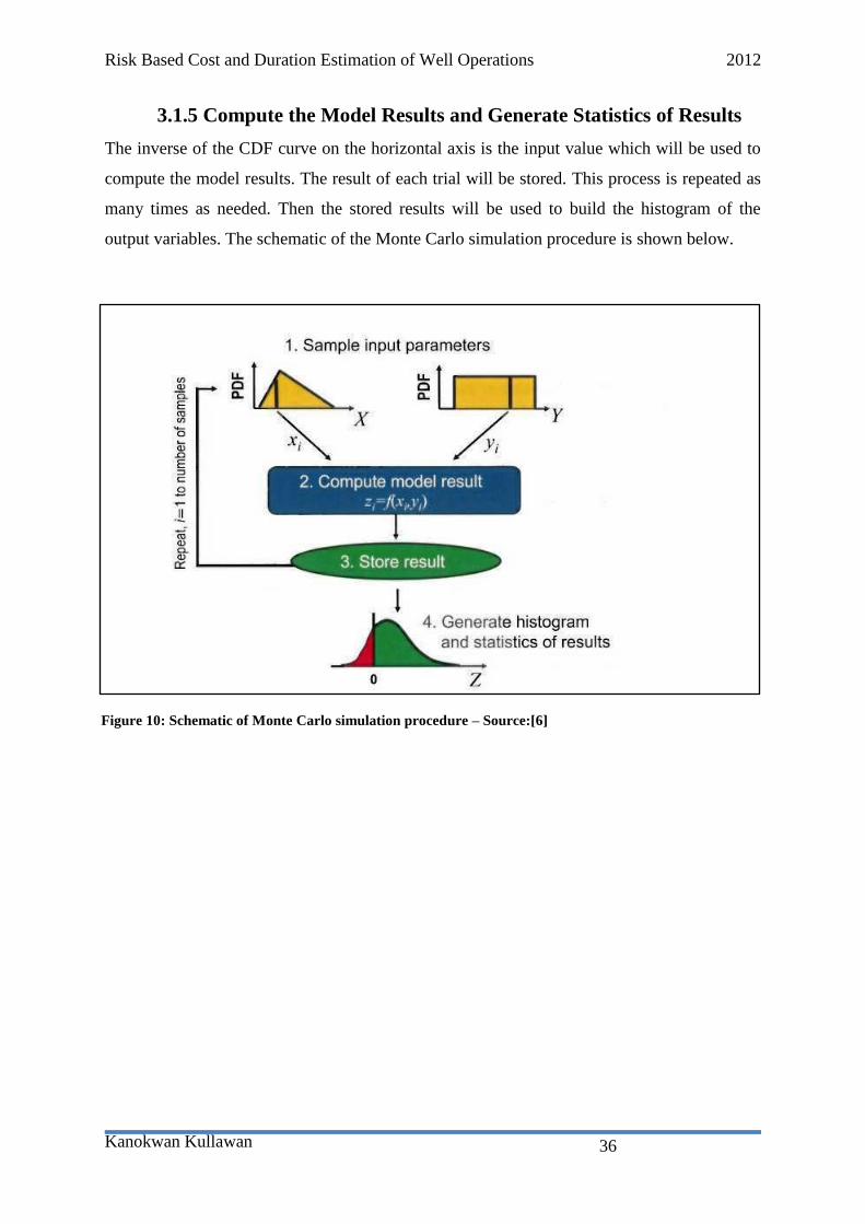
3.1.5 Compute the Model Results and Generate Statistics of Results
The inverse of the CDF curve on the horizontal axis is the input value which will be used to
compute the model results. The result of each trial will be stored. This process is repeated as
many times as needed. Then the stored results will be used to build the histogram of the
output variables. The schematic of the Monte Carlo simulation procedure is shown below.
Figure 10: Schematic of Monte Carlo simulation procedure – Source:[6]

Risk Based Cost and Duration Estimation of Well Operations 2012
Kanokwan Kullawan
37
3.2 Advantages of Monte Carlo Simulation
The Monte Carlo simulation offers a number of advantages as follows: [6]
We have mentioned before that we may not know the exact values of input parameters.
With the MCS technique, the input variable distributions do not require any
approximation.
It is easy to model the correlations and dependencies, based on the assumptions that
they are recognized and well understood.
Typical petroleum engineers and geoscientists have the capability to understand the
level of mathematics used to perform MCS and the complexity of this method.
Solving problems by MCS has less chance of making mistakes compared with an
analytical approach.
There is commercial software available for the tasks involved in the simulation.
Complex and nonlinear mathematics can be included in the model with no extra
difficulty.
Since MCS is widely recognized as a valid technique, the results of this method are
more likely to be accepted by both analysts and decision makers.
The behaviour of the model can be investigated easily.
If there are some changes to the model required, it can be done quickly. Besides, it is
possible to compare the results between before and after the model is changed.

Risk Based Cost and Duration Estimation of Well Operations 2012
Kanokwan Kullawan
38
3.3 Common Pitfalls in Performing Monte Carlo Simulation
Due to a great number of benefits of using Monte Carlo simulations, this technique becomes
the preferred method compared to the deterministic approach for well forecasting. However,
its potential to enhance the reliability of well forecast will be recognized only if the technique
is applied properly. Williamson et al[31]
have presented some observations of common
concerns when using this technique.
Model input should have appropriate level of detail. Based on different situations, the
well can be modelled with the details of the well level, section level or job level.
Depending on how the drilling performance is modelled, the same range of performance
can lead to different overall drilling time. Thus, it is recommended that the input to
MCS model should be basic quantities which are not derived from others. For example,
to model the performance of drilling a hole section with an expected range of ROP is
preferred compared to specifying the expected range of duration of the operation.
It is important to determine the scope of the model correctly by deciding what items to
be included in the model and which events to be ignored. For different well types,
exploration or development, there are different operations which will affect the cost
concerns. It is also important to decide which risk events should be included. A single
well forecast may have less major risks than a multiwell program. Besides, one need to
clarify what level of changes in work scope will invalidate the previous forecast and, at
what level of details, they will be absorbed in the uncertainty of the model inputs. For
example, if the geological objectives have changed, a revision in the well cost estimate
might be required.
There are two pieces of information required in order to have correct results from the
forecast. They are the probability that the well is drilled in the time period in question
(i.e. calendar year) and the probability that well construction is concluded successfully
and not abandoned. If these probabilities are treated as zero, the model will have a build-
in systematic error.
When gathering the data for the simulation, the data set must be large enough to
represent a full range of performance. Additionally, it must include only the data from

Risk Based Cost and Duration Estimation of Well Operations 2012
Kanokwan Kullawan
39
the wells that are similar to the well that is subject to forecasting.
Analysing the data by automatically rejecting the statistical outliers is not a good
method. Investigation of abnormal results may highlight risks and/or opportunities that
call for special attention.
Sometimes poor performances are filtered out from the offset data sets due to the reason
that poor outcomes are treated as specific events that will not occur again. This is not
recommended.
There are some items which can be missing from the work breakdown structure and so
do the cost related to them. These items are often nonrig related, such as, insurance,
corporate allocation and engineering support.
If good offset data is absent, engineers could underestimate the range of possible value
significantly. Even though good offset data is available, there are some common
mistakes associated with parameters selection. The first common error is to define the
minimum and maximum distribution value from the minimum and maximum of the data
value. The extreme values of the input distribution must be wider than the extremes of
the data set. Otherwise, the forecast will be based on the assumption that both the best
case and worst case scenario have already been experienced in the data set. Thus, there
could be an underestimation of uncertainty in the inputs and the predicted results. The
second pitfall is to define the most-likely value from the mean or the median of the data
set. The third pitfall is relying too much on calculated distribution parameters.
In reality, there may be only few offset data points which are available and reliable as an
indication of future performance. With small data set, the uncertainty in the calculated
parameters will be large. This leads to large uncertainty in the predictions as well.

Risk Based Cost and Duration Estimation of Well Operations 2012
Kanokwan Kullawan
40
3.4 Dependencies
In MCS, it is assumed that all the input probability distributions in the model are
independent. However, in reality, the value of a variable can depend on value of others. There
are several methods which can be used to check the dependency of the input parameters. A
common approach is using crossplots of the raw data and calculates the rank correlation
coefficient, known as Spearman’s rank-order correlation coefficient. A correlation value of
+1 means that the two probability distributions are exactly positive correlated. On the
contrary, a correlation value of -1 means that the two probability distributions are exactly
negative correlated. A correlation coefficient of 0 implies that there is no linear relationship
between the two distributions. Positive correlation value, between 0 to +1, produce varying
degrees of positive correlations while negative correlation value, between 0 and -1, produce
varying degrees of inverse correlations.[31],[6]
Some input parameters may be correlated to others since they are influenced by the common
factors. For example, if the hole section takes longer time than expected to drill, the
possibility of encountering problems while running casing of that section could also
increase.[6]
Figure 11: Linear correlation - Source: [6]

Risk Based Cost and Duration Estimation of Well Operations 2012
Kanokwan Kullawan
41
3.5 Example Calculation using Monte Carlo Simulation
Given that the section length to be drilled is 1,000m. Rate of penetration (ROP) of that
section has a triangle distribution with minimum value of 5 m/hr, peak value of 20 m/hr, and
maximum value of 35m/hr. Daily rig rental rate of semisubmersible rig has a uniform
distribution with the minimum value of 4,000,000 NOK and the maximum value of
7,000,000 NOK. The Monte Carlo technique will be performed to estimate the cost of drilling
this section.
Defining the model
To make it simple, the model in this example consists of 2 equations which are:
Drilling time (hr) = section length/ROP
Drilling cost = Drilling time * Rig rental rate/24 + fixed cost
Fixed cost is assumed to be 2,000,000 NOK.
Data gathering and probability distribution selection
Assume that, ROP has a triangle distribution with minimum value of 5 m/hr, peak value of 20
m/hr, and maximum value of 35m/hr. ROP input values drawn from the triangle distribution
is shown below.
Figure 12: Histogram of ROP with normal distribution

Risk Based Cost and Duration Estimation of Well Operations 2012
Kanokwan Kullawan
42
Daily rig rental rate has a uniform distribution ranging from 4 million NOK to 7 million
NOK. Rig rate input values drawn from the uniform distribution are shown below.
.
Randomly sample the input distribution
The input distributions are randomly sampled using 100,000 iterations. The code can be seen
in Appendix.
Compute the model results and generate statistics of results
Figure 13: Histogram of rig rental rate with uniform distribution
Figure 14: Histogram of estimated drilling cost

Risk Based Cost and Duration Estimation of Well Operations 2012
Kanokwan Kullawan
43
From the simulation results, we get an estimation of well cost as shown below:
Average = 14.86 million NOK
Median = 13.43 million NOK
Standard deviation = 5.59 million NOK
In case that there are some events occurring, the duration for well construction would
increase. Here is an example of well time prediction with the risk of major events included. In
this scenario, it is assumed that non-productive time (NPT) from the event has triangle
distribution. The distribution has the minimum value of 2 hr, peak value of 30 and the
maximum of 60 hr. The probability that the event will occur is 0.2. Other parameters are the
same as in the previous example.
Average = 16.28 million NOK
Median = 14.60 million NOK
Standard deviation = 6.48 million NOK
When comparing the results from both cases, we can observe an increase in an estimated
drilling cost in case of included events (represent by its average and median). The
Figure 15: Histogram of estimated drilling cost with the risk of events
included

Risk Based Cost and Duration Estimation of Well Operations 2012
Kanokwan Kullawan
44
uncertainty/spread in the cost estimation is also increasing reflected by the increase in SD.

Risk Based Cost and Duration Estimation of Well Operations 2012
Kanokwan Kullawan
45
3.6 Sensitivity Analysis
Sensitivity analysis (SA) is the study of how the variation in the output of a model (numerical
or otherwise) can be apportioned to different sources of uncertainty. In the beginning,
sensitivity analysis was created to deal with the uncertainties in the input variables and model
parameters. Afterwards, the concept has been developed to combine model conceptual
uncertainty, such as uncertainty in model structures, assumptions and specifications. Thus,
sensitivity analysis (SA) is closely related to uncertainty analysis (UA).[32]
For Monte Carlo simulation, there are uncertainties in input parameters. Hence, it is
important to conduct an analysis to determine the sensitivity of the simulation results to
changes in the estimates of the input parameters.[6]
There are several methods of performing sensitivity analysis. Each technique has its strengths
and weaknesses. One possible way is to divide sensitivity analysis into 3 classes which are
screening method, local SA methods and global SA methods.[32]
For well cost estimation, a graphical method is frequently used as an effective tool for
analyzing sensitivity, such as tornado diagram. Tornado diagram represents the results of a
single-factor sensitivity analysis. Single-factor analysis implies the measurement of effects on
the outcome of each factor, one at a time, while keeping the other parameters at their base
value. One-at-a-time (OAT) approach is the simplest class of screening designs. Besides, one
can also see local SA as a particular case of the OAT approach. OAT designs are classified
into several categories and the tornado diagram is the standard OAT design where one factor
is varied from a standard condition. [32]
Tornado charts deal with single objective and multiple uncertainties. It is used to evaluate the
sensitivity of a single output variable to changes in multiple inputs. It also helps decision
makers to determine 2 decision-driver types: uncertainty drivers and value lever.[6]
Uncertainty drivers are the model-input variables which have the highest impact on the
results. This technique enables quick screening of multiple uncertainties at an early
stage. It also suggests where the budget should be spent on further data collection and
technical analysis.
Value Levers are models input parameters which have most impact on the estimation.

Risk Based Cost and Duration Estimation of Well Operations 2012
Kanokwan Kullawan
46
These can help the team decide which parameters to be focused on in order to optimize
the decision.
Figure 16 shows the result of sensitivity
analysis on the sub operation level of well
construction cost. From this tornado diagram,
mobilization and positioning the rig is the most
important operation regarding the cost. The
figure also shows the ranking of the ten most
important sub-operations.
Figure 16: Cost sensitivity analysis. - Source: [7]

Risk Based Cost and Duration Estimation of Well Operations 2012
Kanokwan Kullawan
47
4. Major Risk Events that Cause Delay
in Well Operations
Well construction cost consists of 2 main parts which are fixed cost and time-related cost.
The latter is a significant part of the total well cost. Thus, accurate forecast of well
construction duration is necessary for budget planning and effective performance
management. There are some major risk events which result from known risks. These events
are considered severe enough to delay the construction process of the well and should be
included in the model for better accuracy of the prediction. Typical major risk events are
described below.
4.1 Kick
Drilling is a process of penetrating into formations. These formations contain fluid under
pressure in pore spaces. Generally, this pressure is overcome by the drilling fluid pressure in
the wellbore which is the result of the hydrostatic pressure and the frictional pressure loss in
the annulus. If the borehole pressure falls below the formation pore pressure, it can lead to
undesirable influx of formation fluid into the wellbore. This event is known as a kick event.
Figure 18: Kick illustration – drill bit hit high -
Source:[5]
Figure 17: Kick illustration – KICK occurring. -
Source:[5]

Risk Based Cost and Duration Estimation of Well Operations 2012
Kanokwan Kullawan
48
4.1.1 Causes of Kick Incidents
Below, some causes that can lead to a kick event are described. [33]
Abnormally high formation pressure is encountered. If formation pressure of these zones
is higher than current mud weight in the well, it will result in a kick event.
Severe lost circulation occurs. This causes the wellbore hydrostatic pressure to decrease
and, as a result, formation fluid enters the wellbore.
Mud weight is too low. When drilling fluid density is too light, mud column cannot
provide enough hydrostatic pressure to overcome the formation pressure. Thus, kick will
occur.
Swabbing effect caused by too high tripping rate out of the well or due to heave effect.
The well is not filled up during pulling out the drillstring.
Circulation of gas cut mud up in the well can lower the hydrostatic pressure below the
formation pore pressure.
Failure to control kick could result in a blowout. In case of blowout, a great deal of effort,
time and money would be required to handle the situation.

Risk Based Cost and Duration Estimation of Well Operations 2012
Kanokwan Kullawan
49
4.2 Stuck pipe
Stuck pipe is the situation where a part of the drillstring, such as drill pipe, drill collar or
BHA, becomes immobile in the hole. The drillstring can neither be rotated nor moved
vertically. This situation can happen during drilling, making connection, testing, logging or
any other operations as long as the drillstring is still in hole. In general, when circulation
stops, the risk of getting stuck increases.
4.2.1 Causes of Stuck Pipe Incidents.
Insufficient hole cleaning: During drilling, cuttings are circulated out of the borehole by
drilling fluid. If the circulation rate is too low and/or the drilling fluid has inappropriate
properties, cuttings will be left in hole. They will settle and accumulate around the
drillstring. This could result in stuck pipe incident. Some notifications of pipe getting
stuck are poor amount of cuttings on shaker and an overpull while tripping.
Wellbore instability: Wellbore instability is an event where some formations become
unstable and the borehole does not maintain its size, shape or structural integrity. Due to
failure in rock mechanisms, fragments of rock fall into the wellbore and accumulate
around drilling BHA. Problems regarding wellbore instability are more common in the
following conditions: [34]
o Shale zones with high percentage of swelling clays such as sodium
montmorillonite.
o Steeply dipping or fractured formations such as limestone.
o Overpressure shale zones.
o Turbulent flow in an annulus leads to washouts situation in soft formations.
Mobile formation[2]
: Mobile formation is caused by overburden stress from the rocks
above squeezes shale or salt into the wellbore. Salt or shale move into the wellbore and
plug the annulus. Hence, the hole becomes undergauge and the drillstring gets stuck.
This could be noticed by an increase in mud chloride content and an overpull during the
connections.
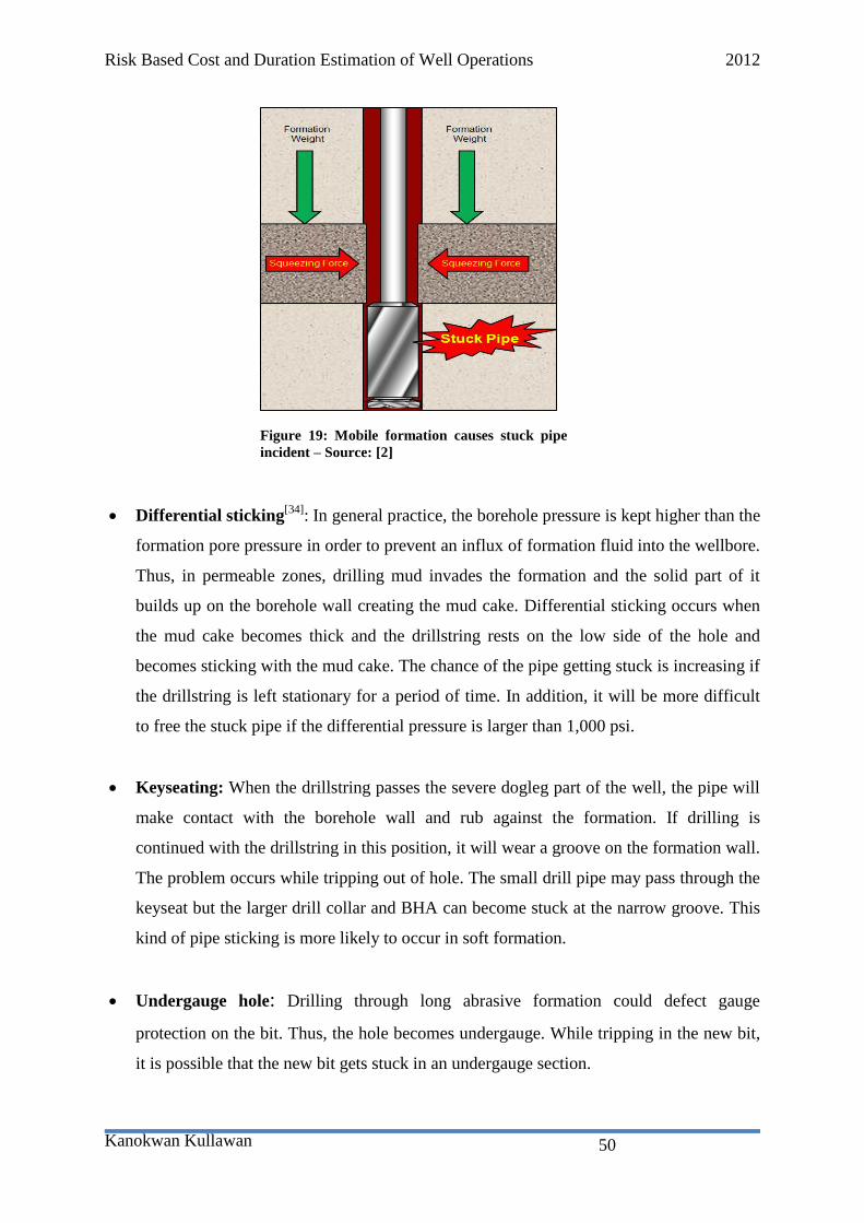
Risk Based Cost and Duration Estimation of Well Operations 2012
Kanokwan Kullawan
50
Differential sticking[34]
: In general practice, the borehole pressure is kept higher than the
formation pore pressure in order to prevent an influx of formation fluid into the wellbore.
Thus, in permeable zones, drilling mud invades the formation and the solid part of it
builds up on the borehole wall creating the mud cake. Differential sticking occurs when
the mud cake becomes thick and the drillstring rests on the low side of the hole and
becomes sticking with the mud cake. The chance of the pipe getting stuck is increasing if
the drillstring is left stationary for a period of time. In addition, it will be more difficult
to free the stuck pipe if the differential pressure is larger than 1,000 psi.
Keyseating: When the drillstring passes the severe dogleg part of the well, the pipe will
make contact with the borehole wall and rub against the formation. If drilling is
continued with the drillstring in this position, it will wear a groove on the formation wall.
The problem occurs while tripping out of hole. The small drill pipe may pass through the
keyseat but the larger drill collar and BHA can become stuck at the narrow groove. This
kind of pipe sticking is more likely to occur in soft formation.
Undergauge hole: Drilling through long abrasive formation could defect gauge
protection on the bit. Thus, the hole becomes undergauge. While tripping in the new bit,
it is possible that the new bit gets stuck in an undergauge section.
Figure 19: Mobile formation causes stuck pipe
incident – Source: [2]

Risk Based Cost and Duration Estimation of Well Operations 2012
Kanokwan Kullawan
51
4.3 Wait on Weather (WOW) or other environmental
interruptions
The ocean environment or sea conditions can have large effect on offshore operation
performance. The effects of winds, rough seas, wave height and other elements can cause
delay in drilling operations. Delays caused by these conditions are commonly referred to as
“waiting on weather”. It is usually calculated as a percentage of total time. Normally, it is
included into the cost prediction models as a variable since the amount of expected WOW
will depend on the time of the year that the operation will take place. [17] ,[35]

Risk Based Cost and Duration Estimation of Well Operations 2012
Kanokwan Kullawan
52
4.4 Downhole tool failure
The bottom hole assemblies (BHA) of the drillstring is composed of many downhole tools
connected to one another. Since BHA failure is one of the largest sources of non-productive
time (NPT), ones might try to minimize the probability of downhole tool failure with several
preventive means. However, prediction of BHA failure is still a complicated problem.
Besides, high weight on bit (WOB) or rotational speed applied to BHA in order to optimize
rate of penetration (ROP) may induce shocks and vibrations on the drillstring. BHA
components could be rapidly destructed due to the operating condition at or close to
resonance. High stresses generated will lead to very short fatigue life. Despite the fact that
there are many factors which cause BHA failure, harmonic vibration, especially lateral
vibration, plays a significant percentage on field failures. Severe downhole vibration can be
responsible for many BHA problems such as: [36],[37]
BHA washouts
Twistoffs
Premature bit failure
Accelerated failure of downhole equipment.
Excessive wear on tool joints
These problems can lead to failure in BHA components and it may require tripping to change
components. In that case, it will lead to extra expenses associated with replacing failed
component and extended rig time. A tripping operation can easily take half a day and, with
the current rig rates, this will represent a significant cost.

Risk Based Cost and Duration Estimation of Well Operations 2012
Kanokwan Kullawan
53
4.5 Lost Circulation
Lost circulation is the reduced or total absence of fluid flow up the annulus when fluid is
pumped through the drillstring. [12]
This reduction of flow may generally be classified as: [38]
Seepage loss – Lost rate is less than 20 bbl/hr (3 m3/hr).
Partial loss – Lost rate is greater than 20 bbl/hr (3 m3/hr) but there are still some
returns.
Total loss – There’s no fluid returns from the annulus.
This incident is detected at surface when the mud return rate from the annulus is less than the
pump rate into the wellbore. Lost circulation occurs when: [39]
1. Extremely high permeability formations are encountered, such as gravel bed or
vugular limestone.
2. A fractured formation is encountered or created due to excessive wellbore pressure.
If the lost circulation incident is severe and the total loss occurs, the hole may not remain full
of fluid even if the pumps are turned on. This leads to reduction in the vertical height of the
fluid column. As a consequence, the pressure exerted on the open formations is reduced.
While the loss zone is taking mud, there can be formation fluid from other zones flowing into
the wellbore creating a crossflow situation. In such a severe situation, a catastrophic loss of
well control could be the result.
Even in the two less severe forms, the loss of fluid to the formation represents a financial loss
that must be dealt with, and the impact of which is directly tied to the per barrel cost of the
drilling fluid and the loss rate over time. Lost circulation is one of the most time consuming
and costly problems associated with the drilling fluid. It has been estimated to cost the
drilling industry over one billion dollars annually in rig time, materials and other financial
resources.
Figure 20: Lost circulation - source:[1]

Risk Based Cost and Duration Estimation of Well Operations 2012
Kanokwan Kullawan
54
4.6 Shallow gas
While drilling top hole section without a riser, the operation is subjected to risk of shallow
fluid flow. This situation is not possible to control by shutting in the well. Influx of shallow
gas into the wellbore is a challenging problem. Most shallow gas kicks result in blowout.
Handling this situation is one of the most complex well control challenges during drilling
operation. Not only serious safety issues regarding operation personnel and rig, shallow gas
blowout can also lead to huge financial losses, especially shallow gas blowout on a platform.
As a consequence, the regulations of some countries require drilling of narrow pilot hole
before opening the hole for the upper casing program.[40],[41]

Risk Based Cost and Duration Estimation of Well Operations 2012
Kanokwan Kullawan
55
5. Simulation Tool
To perform well cost estimation by the probabilistic method, there are several software or
simulation tools being used. Some of the software which is available in the market has been
mentioned in the theory part. In this thesis, the Risk€ software is the simulation tool used for
the well construction time and cost prediction. The description of the software will be based
on [18], the user manual and the explanation given inside the software.
Risk€[18]
is a software developed by International Research Institute of Stavanger (IRIS) with
financial support from ENI. It is a user-friendly tool that provides probabilistic cost and
duration estimation of the well.
5.1 Benefits of Risk€ Software
This is taken from [18].
Makes work processes more effective through:
- Easy to do the calculation in-house
- Easy to automatically generate reports
- Easy to systematize expert input
Facilitates both internal and external communication:
- Can be used for field-to-field comparison
- Can be used for communication in a license setting
- Easy to communicate to decision-makers
Supports technical decisions:
- Risk management in a cost perspective
- Reduce costs and duration related to well construction

Risk Based Cost and Duration Estimation of Well Operations 2012
Kanokwan Kullawan
56
5.2 Applications
The software utilizes Monte Carlo simulation along with sensitivity analysis to help the
decision makers and users determine the overall cost and duration as well as the project
uncertainties. The results from Risk€ also support AFE approval. The total cost and duration
probabilistic estimate of the whole well construction processes is achieved by the summation
of probabilistic cost and duration of all phases and sub operations. This can be described by
two equations shown below.[7]
( 21 )
where C is the total probabilistic cost of the well construction, C1, C2, …, Cn are the costs of
performing sub-operations 1,2, …, n respectively and n is the number of sub-operations.
( 22 )
where D is the total probabilistic duration of the well construction, D1, D2, …, Dn are the
durations of performing sub-operations 1,2, …, n respectively and n is the number of sub-
operations.
Many undesirable events associated with the drilling operations can be added to the
simulation. The results of additional cost and duration from these events are added in the
same manner in the two equations mentioned above.
The simulator divides the well construction processes into phases, i.e. mobilization of drilling
rig, spudding of the well, BOP installation, drilling hole sections and well abandonment. User
provides input regarding probability distribution type and value of each parameter. The
software will simulate the result of the standard operation plan based on user input. The user
can also specify if 10,000 or 100,000 iterations are required for the Monte Carlo simulation.

Risk Based Cost and Duration Estimation of Well Operations 2012
Kanokwan Kullawan
57
5.3 Input of Drilling Phases for Generation of Standard
Operation Plan
Once a well is created in Risk€ and its drilling environment has been identified, the next step
is to describe the well architecture. After that, the user will work with the well standard
operation plan and the risk operation plan. In Risk€, the standard operation plan is the plan
for drilling activities without any undesirable events.
The Risk€ software divides the well operations into 5
main phases which are:
Mobilization Phase
Spudding Phase
BOP Installation Phase
Drilling Phase
Abandonment Phase
Each phase consists of a list of sub operations, both
automatically generated from the software and manually
added by the user.
In the input panels, user chooses the type of probability
distribution for cost and duration of each sub operations.
The technology applied in the operation is also selected.
Here are some input panels of each operation phase.
Figure 21: Snapshot of operation plan
automatically created in RiskE

Risk Based Cost and Duration Estimation of Well Operations 2012
Kanokwan Kullawan
58
5.3.1 Well Architecture
The well architecture is an editor for the casing description of each section, including the
length and diameter of an open hole section. The details related to casing shoe depth, casing
hanging point, casing outer diameter (casing OD), and casing inner diameter (casing ID) are
specified here. From that information, a wellbore schematic of the well to be simulated can
be drawn.
5.3.2 Mobilization of drilling rig
In this panel, the user needs to specify the technology used for rig mobilization on the left
hand side of the panel. Each rig mobilization technology requires different input information.
The classes of technology which are available for choosing in this software and its input are
listed in the table shown below:
Figure 22: Input panel for well architecture

Risk Based Cost and Duration Estimation of Well Operations 2012
Kanokwan Kullawan
59
Mobilize Rig Technology Information Required
Mobilize Rig Jack Up
Distance to location, Moving velocity, Duration for
positioning rig, Jack up distance and velocity, Cantilever
distance and velocity
Mobilize Rig Platform Distance to skid rig, skidding velocity
Mobilize Rig Land Rig Distance to location, Moving velocity, Rig up duration,
Distance to skid rig, Skidding velocity
Mobilize Rig Semi Sub Distance to location, Moving velocity, Duration for
positioning rig, Anchoring duration
Mobilize Rig Floater Distance to location, Moving velocity, Positioning rig
duration
Table 2: Mobilize rig technology and its input information – Source:[42]
In every phase, there is an input panel for cost related information. In this panel, there are 6
types of cost related information which need to be filled in which are:
Rig rate - The cost rate of the rig that is used for the well construction.
Drillstring/BHA costs - The cost rate for the drillstring including the bottom hole
assembly.
Fixed cost – Fixed cost related to: Site survey, Rig positioning, Rig mobilization/
demobilization, Vessels mobilization/demobilization, different types of logging (e.g.
electric logging, cased hole logging), Insurance, Fishing and abandon services, Well
planning.
Spread rate – The sum of the cost related to: Vessels, Additional (catering etc),
Cement services and personnel, Mud logging, Conductor driving equipment, Dock
fees & base overheads, Rental tools, Consultants on rig, ROV, Water, Fuel (including
rig and vessels).
Wellhead cost - The fixed cost for the wellhead for the phase taken into consideration.
Support cost - The cost rate related to: Drilling Office overhead, Office Support
consultant, Other drilling expenses, Air transport

Risk Based Cost and Duration Estimation of Well Operations 2012
Kanokwan Kullawan
60
5.3.3 Spudding
Spudding phase is an operation being conducted in an early stage of drilling a new well. This
is where we drill the top hole for installing a conductor which would form the fundament for
the rest of the well. There are 3 main technologies for making this top hole and run the
conductor. Jetting is the technology where a high-velocity and high-pressure fluid stream is
used to make hole in the ground before the conductor can be run. Hammering means that the
conductors are hammered down into the ground without drilling the hole first. Top hole refers
to the methodology of drilling the hole first, then running the conductor.
Spudding Technology Information Required
Jetting Time to MU and break jet assemblies, RIH and POOH speed
Hammering Time to rig up and rig down
Top Hole Time to MU and break BHA, RIH and POOH speed, ROP, Bit cost
Table 3: Spudding technology and its input variables
Figure 23: Mobilization phase input panel.

Risk Based Cost and Duration Estimation of Well Operations 2012
Kanokwan Kullawan
61
5.3.4 Drilling hole sections
The input panel shown below is used for generating the different drilling phases in a well,
e.g. drilling and casing setting of surface section 26”, 12 ¼”,and 8 ½”.
Figure 24: Spudding Phase Input Panel

Risk Based Cost and Duration Estimation of Well Operations 2012
Kanokwan Kullawan
62
5.3.5 BOP Editor
For BOP editor, there’s only one difference between installing BOP at surface and sea bed.
On a platform well, the BOP will be on surface. When using a semisubmersible rig and
drilling in deep water, the BOP will be installed on seabed. In case of subsea BOP, the time
required to run BOP and riser is added.
Figure 25: Drilling phase input panel

Risk Based Cost and Duration Estimation of Well Operations 2012
Kanokwan Kullawan
63
5.3.6 Distribution Mode Input
Users can choose which type of distribution is the most suitable for that parameter. This
could be based on expert judgments and/or historical data. The common distribution types
used are single value distribution, uniform distribution, triangle distribution, piecewise linear
distribution and discrete distribution. However, more advanced distributions such as generic
distribution, Gaussian distribution, exponential distribution and Weibull distribution are also
available in this software. The generic distribution mentioned here refers to the distribution
which the distribution curve is constructed based on a set of data. This distribution type is
suitable when it is difficult to define the distribution type and the historical data is available.
Figure 27: Distribution Mode Input Panel
Figure 26: BOP editor input panel
Risk Based Cost and Duration Estimation of Well Operations 2012
Kanokwan Kullawan
64
5.4 Input of Risk Events for Generation of Risk Operation Plan
Risk operation plan is the operation plan where the effects of undesirable events are included
in the prediction. The consequences of these risks are reflected in the predicted results which
could be compared with the risk free operation plan.
The risks associated with drilling activities can be categorized as events in the well level or
events in phase level. The user defines extra duration and cost caused by the events and then,
specifies the probability of occurrence.
5.4.1 Risk Events in Well Level
Risk events in the well level refer to any undesirable events which can occur throughout the
well construction processes, not limited to any operation phases. Some examples of risk
events, taken from the Risk€ library description and the software user manual, in well level
are:
Wait on weather - Delays due to bad weather stopping operations on rig. Typically
strong winds will prevent using cranes etc.
Wait on rig repair - Time and money spent repairing the rig. The duration is only
when operations has to be stopped because of the repairs.
Wait on material - Operations will be delayed if the correct materials are not present
on the rig at the needed time.
Drawwork failure - Drawwork failure will delay operations.

Risk Based Cost and Duration Estimation of Well Operations 2012
Kanokwan Kullawan
65
5.4.2 Risk Events in Phase Level
In each operation phase, there are some phase specific risks. These events are related to the
activities being conducted in that phase and not likely to occur during other phases. Here are
some examples of undesirable events in each phase.[42],[43]
Mobilization Phase
Tug vessel problems - A vessel tugging the rig to position has a problem (e.g. engine
failure, propeller failure etc.) causing delay. Is most relevant when moving the rig to
location and also when positioning the rig.
Interference with subsea facilities - Existing structures on the seabed, such as
Figure 28: Input panel for risk events in well level

Risk Based Cost and Duration Estimation of Well Operations 2012
Kanokwan Kullawan
66
flowlines, jumpers or shipwrecks, can be encountered during anchoring and spudding
operations. This can cause delays and may also cause damage to the facilities and/or
rig.
Anchor handler vessel problems - The vessels used during the anchoring encounter
problems such as vessel is inadequate for the task, engine failure or propeller failure.
These problems will cause delays during the anchoring operation.
Currents - Strong currents might cause delays, particularly when positioning the rig.
Weather - This event covers weather effects not included in wait on weather, but can
cause specific problems during the mobilize rig phase.
Spudding[42],[43]
Poor visibility at seabed - If the visibility of the seabed is poor, lowering the jetting
tool to the correct location on the seabed might take some extra time.
Stuck conductor - During jetting the conductor the conductor can become stuck when
the jetting progress stops, and it might be impossible to move/retrieve the conductor
due to excessive friction and over pull. The delay caused by this will vary between
working the conductor free and re-spudding the well.
Conductor inclination problems - The conductor can be spudded at an unacceptable
inclination. Too high inclination of the conductor can create problems landing
wellhead and/or BOP, and could cause internal casing wear and additional bending
forces / load and wear on the connectors, BOPs and/or riser. In some cases a re-spud
is necessary.
ROV failure - The ROV has problems causing delays when setting the conductor.
Drilling[42],[43]
Stability/Collapse problems - Collapse of the hole can lead to stuck pipe, stuck casing,
unable to extend casing point to desired depth. It can occur due to seawater drilling
fluid and long open hole section. Additional time for circulating, reaming and wiper
trips must be expected.
Shallow gas - Shallow gas can be encountered while drilling the hole sections just
below sea bed. Presence of shallow gas can result in an uncontrolled flow of gas

Risk Based Cost and Duration Estimation of Well Operations 2012
Kanokwan Kullawan
67
endangering the hole, the rig and the personnel.
Stuck casing - During running casing the string can become stuck above the setting
depth. Subsequently the hanger will be above the well head and cannot be set.
Packoff - During running casing and cementation pack off, i.e. plugged wellbore
around the drillstring, can occur. This can happen for a variety of reasons, the most
common being that either the drilling fluid is not properly transporting cuttings and
cavings out of the annulus or portions of the wellbore wall collapse around the
drillstring. When the well packs off, there is a sudden reduction or loss of the ability
to circulate, and high pump pressures follow. If prompt remedial action is not
successful, expensive episodes of stuck pipe or lost well and re-spud might be the
result.
Improper cement job - If the casing is not well enough cemented to the formation,
actions must be taken to better cement the casing. Typical actions include squeeze
cementing.
MWD/LWD/BHA failure - If the measurement devices fails, extra time will be spent
either drilling slower, re-log section or trip out to fix the problem. The time will
depend on when the failure occurs, from at rig floor to when you are drilling.
Stuck pipe - If the pipe gets stuck due to for example mechanical sticking, differential
sticking or pack off, effort must be taken to attempt to pull it loose.
BOP[42],[43]
Currents - Strong currents can prevent running the BOP stack, and also using ROV.
BOP/Riser equipment problems - BOP and riser equipment problems resulting in
waiting to run the BOP's or waiting to land the BOP because of bad weather. BOP
stack problems revealed during the testing of the BOP system resulting in pulling the
BOP and repair and re-test at the rig.
Unable to pressure test BOP - Unable to pressure test the BOP due to problems with
seals on test tool or wellhead connector. Max time is to pull and rerun the BOP.
Additional time to repair and possible extra time to transport spare part from shore to
the rig might also be needed.
Poor visibility at seabed - Poor visibility leads to delays due to difficulties to observe
operations at seabed.

Risk Based Cost and Duration Estimation of Well Operations 2012
Kanokwan Kullawan
68
Abandon[42],[43]
Cement unit/job problems - Cement unit problems during the job or bulk cement,
spacer and mix water delivery, air compressors, etc.
Inability to set cement plug - Contaminated cement or non-adequate pumping
schedule might prevent setting the cement plug. The cement plug can also be set in
the wrong place whereas it has to be reset, or the cement does not harden properly.
Weather - Weather effects not causing wait on weather, but impede the abandonment
operations in other ways.
Figure 29: Input panel for risk events in phase level

Risk Based Cost and Duration Estimation of Well Operations 2012
Kanokwan Kullawan
69
After all the associated risks are added to standard operation plan, a risk operation plan is
generated. Thus, the result of risk operation plan can be simulated and compared with the
result of the standard operation plan.
Figure 30: Snapshot of risk
operation plan

Risk Based Cost and Duration Estimation of Well Operations 2012
Kanokwan Kullawan
70
5.5 Simulation Results
The simulator offers probabilistic results from both the standard operation plan and the risk
operation plan. The latter case is available when the user has included the risk events in the
standard operation plan. The results of cost and duration are presented as probability density
function in a histogram shape. The main results provided by the simulator are:[18]
Curves representing the mean duration and the mean cost, obtained analytically from
the input distributions versus the deterministic drill depth.
Drill depth versus time curves.
The probability distribution for the total drilling cost and duration is given using a
histogram, including summary statistics such as the maximum values, mean, and
standard deviation.
The probabilities of performing the well construction within user defined cost and
time limits.
Sensitivity analysis based on correlation coefficients
Sensitivity analysis based on cost and duration contribution
Cost breakdown
Comparison of different well design
Sensitivity analysis on phases, operations and events level
Figure 31: Well summary result

Risk Based Cost and Duration Estimation of Well Operations 2012
Kanokwan Kullawan
71
Figure 32: Result view of phase sensitivity
Figure 33: Result of operation sensitivity

Risk Based Cost and Duration Estimation of Well Operations 2012
Kanokwan Kullawan
72
The total cost of the standard operation plan can be broken down into different cost codes and
displayed in the cost breakdown panel. The user can choose if either the cost of the total well
or the selected phase will be shown.
Figure 34: Result view of cost breakdown
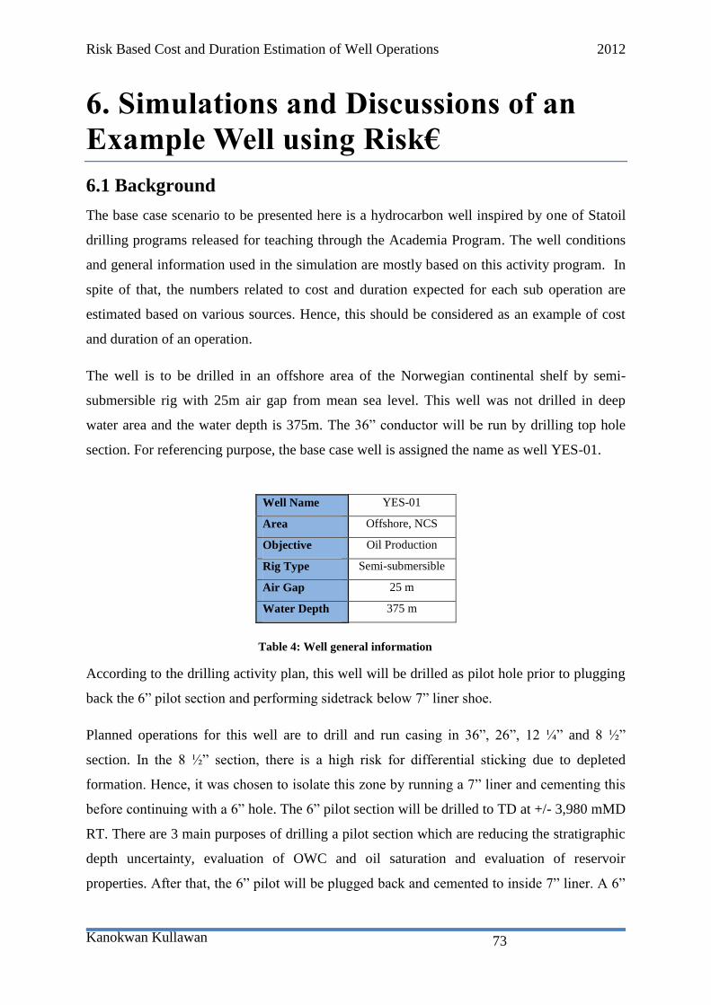
Risk Based Cost and Duration Estimation of Well Operations 2012
Kanokwan Kullawan
73
6. Simulations and Discussions of an
Example Well using Risk€
6.1 Background
The base case scenario to be presented here is a hydrocarbon well inspired by one of Statoil
drilling programs released for teaching through the Academia Program. The well conditions
and general information used in the simulation are mostly based on this activity program. In
spite of that, the numbers related to cost and duration expected for each sub operation are
estimated based on various sources. Hence, this should be considered as an example of cost
and duration of an operation.
The well is to be drilled in an offshore area of the Norwegian continental shelf by semi-
submersible rig with 25m air gap from mean sea level. This well was not drilled in deep
water area and the water depth is 375m. The 36” conductor will be run by drilling top hole
section. For referencing purpose, the base case well is assigned the name as well YES-01.
Table 4: Well general information
According to the drilling activity plan, this well will be drilled as pilot hole prior to plugging
back the 6” pilot section and performing sidetrack below 7” liner shoe.
Planned operations for this well are to drill and run casing in 36”, 26”, 12 ¼” and 8 ½”
section. In the 8 ½” section, there is a high risk for differential sticking due to depleted
formation. Hence, it was chosen to isolate this zone by running a 7” liner and cementing this
before continuing with a 6” hole. The 6” pilot section will be drilled to TD at +/- 3,980 mMD
RT. There are 3 main purposes of drilling a pilot section which are reducing the stratigraphic
depth uncertainty, evaluation of OWC and oil saturation and evaluation of reservoir
properties. After that, the 6” pilot will be plugged back and cemented to inside 7” liner. A 6”
Well Name YES-01
Area Offshore, NCS
Objective Oil Production
Rig Type Semi-submersible
Air Gap 25 m
Water Depth 375 m

Risk Based Cost and Duration Estimation of Well Operations 2012
Kanokwan Kullawan
74
oil producer will be kick off below 7” liner shoe and geo-steered to TD at +/- 4,083 mMD
RT. The information regarding each section is presented in table 5 .
Section Section depth Suspension Depth Casing shoe Casing OD Casing ID
(in) (mMD) (mMD) (mMD) (in) (in)
36.00 460 400 457 30.000 29.000
26.00 1352 400 1347 20.000 19.000
12.25 3161 400 3155 9.625 8.844
8.50 3408 3055 3408 7.000 6.188
6.00(pilot) 3980 - - - -
6.00(producer) 4083 - - - -
Table 5: Section details
Figure 35 shows the wellbore schematic of the pilot hole for the well YES-01. The numbers
shown in the figure are section TD of 26”, 12 ¼”, 8 ½” and 6” pilot section respectively.
The operation plan of this well is to divide drilling activities into steps as shown below.
Mobilization
Move to position
Position rig
Anchoring
Figure 35: Wellbore schematic of
pilot hole
3,980.00m

Risk Based Cost and Duration Estimation of Well Operations 2012
Kanokwan Kullawan
75
Spudding
MU BHA
RIH
Drill top hole
POOH
Break BHA
Run conductor
Cement
POOH
Drilling 26" Section
MU BHA
RIH
Drill
Circulate
POOH
Break BHA
Run casing
Cement
POOH
BOP
Nipple up BOP
Run BOP and riser
Pressure test BOP
Drilling 12 1/4" section
MU BHA
RIH
Drill new formation
Circulate
LOT
Drill
Circulate
POOH
Change bit
RIH
Drill
Circulate
POOH
Break BHA
Run Casing
Cement

Risk Based Cost and Duration Estimation of Well Operations 2012
Kanokwan Kullawan
76
POOH
BOP
Pressure test BOP
Drilling 8 1/2" section
MU BHA
RIH
Drill new formation
Circulate
LOT
Drill
Circulate
POOH
Break BHA
Run casing
Cement
POOH
BOP
Pressure test BOP
Drilling 6" pilot section
MU BHA
RIH
Drill
Circulate
POOH
Break BHA
Plug back pilot hole
RIH with 3 ½” cement stinger
Plug back pilot hole to inside 7” liner
POOH 3 ½” cement stinger
Sidetracking
MU BHA
RIH
Drill
Circulate
POOH
Break BHA
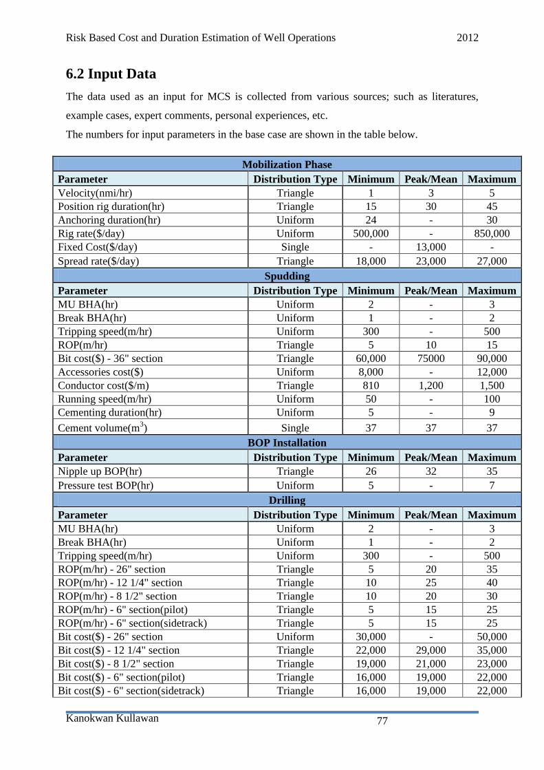
Risk Based Cost and Duration Estimation of Well Operations 2012
Kanokwan Kullawan
77
6.2 Input Data
The data used as an input for MCS is collected from various sources; such as literatures,
example cases, expert comments, personal experiences, etc.
The numbers for input parameters in the base case are shown in the table below.
Mobilization Phase
Parameter Distribution Type Minimum Peak/Mean Maximum
Velocity(nmi/hr) Triangle 1 3 5
Position rig duration(hr) Triangle 15 30 45
Anchoring duration(hr) Uniform 24 - 30
Rig rate($/day) Uniform 500,000 - 850,000
Fixed Cost($/day) Single - 13,000 -
Spread rate($/day) Triangle 18,000 23,000 27,000
Spudding
Parameter Distribution Type Minimum Peak/Mean Maximum
MU BHA(hr) Uniform 2 - 3
Break BHA(hr) Uniform 1 - 2
Tripping speed(m/hr) Uniform 300 - 500
ROP(m/hr) Triangle 5 10 15
Bit cost($) - 36" section Triangle 60,000 75000 90,000
Accessories cost($) Uniform 8,000 - 12,000
Conductor cost($/m) Triangle 810 1,200 1,500
Running speed(m/hr) Uniform 50 - 100
Cementing duration(hr) Uniform 5 - 9
Cement volume(m3) Single 37 37 37
BOP Installation
Parameter Distribution Type Minimum Peak/Mean Maximum
Nipple up BOP(hr) Triangle 26 32 35
Pressure test BOP(hr) Uniform 5 - 7
Drilling
Parameter Distribution Type Minimum Peak/Mean Maximum
MU BHA(hr) Uniform 2 - 3
Break BHA(hr) Uniform 1 - 2
Tripping speed(m/hr) Uniform 300 - 500
ROP(m/hr) - 26" section Triangle 5 20 35
ROP(m/hr) - 12 1/4" section Triangle 10 25 40
ROP(m/hr) - 8 1/2" section Triangle 10 20 30
ROP(m/hr) - 6" section(pilot) Triangle 5 15 25
ROP(m/hr) - 6" section(sidetrack) Triangle 5 15 25
Bit cost($) - 26" section Uniform 30,000 - 50,000
Bit cost($) - 12 1/4" section Triangle 22,000 29,000 35,000
Bit cost($) - 8 1/2" section Triangle 19,000 21,000 23,000
Bit cost($) - 6" section(pilot) Triangle 16,000 19,000 22,000
Bit cost($) - 6" section(sidetrack) Triangle 16,000 19,000 22,000

Risk Based Cost and Duration Estimation of Well Operations 2012
Kanokwan Kullawan
78
Parameter Distribution Type Minimum Peak/Mean Maximum
Circulation time(hr) Uniform 4 - 7
Fluid cost($/m3) Uniform 1000 - 2000
Casing cost($/hr) - 26" section Triangle 300 365 420
Casing cost($/hr) - 12 1/4" section Triangle 130 150 170
Casing cost($/hr) - 8 1/2" section Triangle 90 105 120
Casing run speed(m/hr) Single 300 300 300
Cementing duration(hr) - 26" section Triangle 7 9 11
Cementing duration(hr) - 12 1/4" section Triangle 10 12 14
Cementing duration(hr) - 8 1/2" section Triangle 13 15 18
Cement volume(m3) - 26" section Single 132.44 132.44 132.44
Cement volume(m3) - 12 1/4" section Single 11.64 11.64 11.64
Cement volume(m3) - 8 1/2" section Single 5.30 5.30 5.30
Cement slurry cost($/m3) Single 2000 2000 2000
Leak off test duration(hr) Uniform 0.5 - 1.5
Rig rate($/day) Uniform 500,000 - 850,000
Drillstring/BHA cost($/day) Normal - 50,000 -
Fixed Cost($/day) Single 60,000 60,000 60,000
Spread rate($/day) Triangle 60,000 80,000 100,000
Support Cost($/day) Uniform 50,000 - 80,000
Wellhead cost($) Single 800,000 800,000 800,000
Table 6: Summary of input parameters

Risk Based Cost and Duration Estimation of Well Operations 2012
Kanokwan Kullawan
79
6.3 Results from Standard Operation Plan
Standard operation plan is referred to the well construction processes where all the activities
can be performed according to the planned schedule, without any interruptions from
undesirable events.
After all the input parameters have been filled in, user can choose either 10,000 or 100,000
iterations to be used for the Monte Carlo simulation. In this case, 10,000 iterations are used
for the simulation. The results from the simulation will be presented in various forms.
6.3.1 Deterministic View
An overall result for an operation plan can be displayed in a deterministic view. The results
are based on expected values in the probability distributions that are given for the different
input values. Simulation is not needed to display this type of result.
From figure 36, the time-depth curve (the blue line) demonstrates that it takes 29.09 days to
reach the TD of the well. By including circulation, tripping and breaking BHA time, it
requires about 29.97 days of well duration. The red line shows the construction cost as the
well is drilled deeper. To finish drilling this well, a budget around 30.01 million USD is
required, according to the deterministic well cost estimation.
Figure 36: Deterministic view from the result of the standard operation plan

Risk Based Cost and Duration Estimation of Well Operations 2012
Kanokwan Kullawan
80
6.3.2 Probabilistic View
After performing the Monte Carlo simulation, the probabilistic results can be shown.
Well Summary
The well summary view displays the time – depth curve in the form of different percentiles.
At the bottom part of the display, it shows the histograms for total cost and duration of the
well construction processes. The expected value, standard deviation as well as possible range
of outcome are also presented here.
From figure 37, the expected duration to drill this well is 29.78 days with the standard
deviation of 1.58 days. An expected cost of this well is 29.90 million USD with the standard
operation of 1.77 million USD. The well could be completed within 25.75 days the soonest
and 37.33 days the latest. The budget required to drill this well could range from 24.53 –
37.51 million USD. The probability that the operation will be completed within 29.78 days is
54.4% and the probability that the operation will cost at most 29.90 million USD is 53.1%.
Method Deterministic Approach Probabilistic Approach
Expected Duration 28.71 days 29.78 days
Range of Possible Duration N/A 25.75 - 37.33 days
Expected Cost 30.01 million USD 29.90 million USD
Range of Expected Cost N/A 24.53 - 37.51 million USD
Table 7: Results comparison between deterministic and probabilistic approach
Figure 37: Well summary result from standard operation plan

Risk Based Cost and Duration Estimation of Well Operations 2012
Kanokwan Kullawan
81
From table 7, the expected value of cost and duration required for well operation from both
approaches are not the same, but they do not have huge differences. However, the
deterministic method is not able to provide the range of possible outcome as well as the
probability of completing the well within the expected time period and budget.
Phase Sensitivity
This view will display the contribution of each phase to the estimated results. Each phase’s
cost and duration is displayed as proportions of the total cost and duration for the operation
plan.
The phase sensitivity analysis shows that drilling 12 ¼” section is the most sensitive phase
compared to the other phases. It contributes for 27% of the total cost and 24% of the total
duration. Drilling phases for several sections as well as mobilization phase also contribute
significantly to the total estimated cost and duration. The differences between these phases
are not apparent. One can notice from figure 38 that the mobilization phase makes the second
largest contribution to the total duration but the 6th
largest contribution to the well total cost.
This could be based on the fact that during the time of rig mobilization, the spread rate cost is
considerably lower than other phases in this example case.
Figure 38: Phase sensitivity from standard operatoin plan

Risk Based Cost and Duration Estimation of Well Operations 2012
Kanokwan Kullawan
82
Operation Sensitivity
The operation sensitivity displays each operation’s cost and duration as proportions of the
total cost and duration.
When looking at the operation level, drilling sub operations are the most dominating factors
compared to other sub operations. Both cost and duration sensitivity analysis demonstrate
that drilling the sidetrack hole section has the largest effect on the results. Cost and duration
spent on drilling other sections also have significant impact and slight difference can be
observed among various sections.
Cost Breakdown
The cost breakdown result type shows the expected total cost, broken into predefined cost
categories (cost codes) for the standard operation plan.
Figure 39: Operation sensitivity from standard operation plan

Risk Based Cost and Duration Estimation of Well Operations 2012
Kanokwan Kullawan
83
If we break down the well total cost into its elements, it is obvious that the rig rental cost has
the most important contribution to the total cost. It is responsible for 20.10 million USD from
29.89 million USD of total well cost or more than 67% of the well total cost. The second
largest contribution is the spread rate cost which highly depends on the total well duration as
well. The spread rate represents 14.78% of the well total cost. These 2 cost codes are
responsible for 82.01% of the total cost. Both of them are time-related cost. Thus, we can
conclude that time spent on well operations is the most crucial cost driving parameter.
Figure 40: Cost Breakdown of standard operation
plan

Risk Based Cost and Duration Estimation of Well Operations 2012
Kanokwan Kullawan
84
6.4 Detailed Sensitivity Analysis
According to the tornado charts of phase sensitivity and operation sensitivity of the base case
result (figure 38 and figure 39), time and cost spent on drilling and mobilization has the
largest contributions on the total well cost and duration. Within the drilling phase, time spent
on drilling is the most influential parameter while moving rig to location has the greatest
impact on mobilization phase. As a consequence, 2 input variables, which are ROP and rig
moving velocity, have been selected for detailed analysis here. The result of the detailed
sensitivity analysis could suggest how an exact knowledge of these parameters would affect
the reduction in uncertainty of the total cost and duration. It could also recommend if budget
should be spent on further data collection.
6.4.1 Detailed Analysis of ROP
Drilling the formation takes much more time than tripping, circulation, casing running and
cementing. Thus, further study has been performed to analyse the effect of various ROP
inputs on the uncertainty and expected value of the prediction.
Uncertainty Analysis
In order to analyse the uncertainty of the results, the standard deviation of well cost and
duration obtained by using different distribution types for ROP will be plotted against the
standard deviation obtained while using single value input for the ROP. The distribution
types to be studied here are the uniform distribution, the triangle distribution and the single
distribution. Each distribution type will be assigned for every section. The results of the
uniform distribution mean that the uniform distribution is used as an input distribution for
ROP in every section. Same logic goes to the triangle distribution and the single distribution.
The ROP input values used in this study are shown in the table below.
Triangle Distribution
Section(in)
ROP (m/hr)
Minimum Most
Likely Maximum
26.00 5 20 35
12.25 10 25 40
8.50 10 20 30
6.00(pilot) 5 15 25
6(ST) 5 15 25

Risk Based Cost and Duration Estimation of Well Operations 2012
Kanokwan Kullawan
85
Uniform Distribution
Section(in)
ROP (m/hr)
Minimum Most
Likely Maximum
26.00 5 - 35
12.25 10 - 40
8.50 10 - 30
6.00(pilot) 5 - 25
6(ST) 5 - 25
Single Distribution
Section(in)
ROP (m/hr)
Minimum Most
Likely Maximum
26.00 - 20 -
12.25 - 25 -
8.50 - 20 -
6.00(pilot) - 15 -
6(ST) - 15 -
Table 8: ROP input values for each distribution type.
Well Duration Analysis: The effect of each distribution type on the uncertainties of
well duration is shown by the standard deviation of the predicted duration.
Distribution
Type
Duration SD
(days)
Triangle 1.60
Uniform 2.43
Single 0.73
Table 9: Well duration SD for each ROP distribution type
Figure 41: Uncertainties in well duration for different ROP
distribution

Risk Based Cost and Duration Estimation of Well Operations 2012
Kanokwan Kullawan
86
From table 9 and figure 41, it is obvious that the single distribution ROP gives the results
with the least uncertainties in well duration while the uniform distribution gives the results
with the largest uncertainties. The difference between each distribution type is pretty
apparent. The well duration standard deviation from the uniform distribution and the triangle
distribution are 3.3 and 2.2 times higher than the single distribution.
Well Cost Analysis: Similar to the well duration, in this case, the SD of estimated
well cost will be compared for each distribution type.
Distribution
Type
Cost SD(million
USD)
Triangle 1.79
Uniform 2.41
Single 1.22
Table 10: Well cost SD for each ROP distribution type
The uncertainties in the well cost have a matching results with the uncertainties in well
duration. From table 10 and figure 42, we can notice that the single distribution and the
uniform distribution also give the lowest and the highest uncertainties result respectively.
Nevertheless, the difference in well cost uncertainties is smaller than the well duration
uncertainties. The standard deviation of the well cost from the uniform distribution and the
triangle distribution are 2.0 and 1.5 times higher than the single distribution.
From the uncertainties analysis of the well cost and duration, we can conclude that better
knowledge on expected range of ROP could greatly reduce the uncertainties of the results.
Figure 42: Uncertainties in well cost for different ROP
distribution

Risk Based Cost and Duration Estimation of Well Operations 2012
Kanokwan Kullawan
87
Value Analysis
In this section, the expected value of the results will be analysed by varying the ROP. In
every section, the ROP will be set as single distribution. 3 more cases will be simulated and
compared with the triangle distribution based case. These 3 cases are when the ROP is at its
minimum, at its most likely and at its maximum. The inputs ROP for each section are shown
in the table below. “Minimum” mentioned in the table and figure below implies that the ROP
input value in every section is at its minimum using the single distribution. Same logic is
used for the “Most Likely” and “Maximum” cases.
ROP (m/hr)
Section (in) 26.00 12.25 8.50 6.00(pilot) 6.00(ST)
Minimum 5 10 10 5 5
Most Likely 20 25 20 15 15
Maximum 35 40 30 25 25
Table 11: ROP inputs for value analysis
Well Duration Analysis
ROP(m/hr) Expected Duration
(days)
Minimum 46.93
Most Likely 29.16
Maximum 25.64
Base Case 29.90
Table 12: Expected duration from different ROP value
Figure 43: Expected well duration for different ROP value

Risk Based Cost and Duration Estimation of Well Operations 2012
Kanokwan Kullawan
88
In the uncertainties analysis section, the results from the triangle distribution and the single
distribution have a large difference in their standard deviation of duration. However, from
table 12 and figure 43, we can see that the difference between the expected well duration
from the “Most Likely” case (single distribution) and the “Base Case” (triangle distribution)
is almost negligible. The “Most Likely” case is only 0.82 day faster than the “Base Case”. On
the other hand, the change in ROP from “Base Case” to “Minimum” and “Maximum” case
has a noticeable effect on the well duration. If the ROP of every section is at its minimum, the
well can be expected to be delayed more than 50% compared to its initial prediction.
Well Cost Analysis
ROP(m/hr) Expected Cost(million
USD)
Minimum 44.82
Most Likely 29.36
Maximum 26.31
Base Case 30.06
Table 13: Expected well cost from different ROP Value
Similar to the well duration, the expected cost from the “Most Likely” case and the “Base
Case” are almost the same. The “Most Likely” cost is 0.7 million USD lower than the “Base
Case”. When the ROP is at its minimum, it causes a long delay in the well duration. Thus, the
expected cost is also increased significantly. At the same time, when the ROP is at its
maximum, the reduction in well cost is detectable but the effect is not as large as the
minimum case.
Figure 44: Expected well cost for different ROP value

Risk Based Cost and Duration Estimation of Well Operations 2012
Kanokwan Kullawan
89
6.4.2 Detailed Analysis of Rig Mobilization Velocity
As presented in the phase sensitivity tornado
chart, figure 38, mobilization phase is the 2nd
most influential phase on the well duration.
Apart from that, the article “Who moved my
rig?” published in Oil & Gas Financial Journal
published on December 1st, 2011 presented a
study on this which was performed by Alvarez
and Marsal 2009. The summary of the study
showed that rig mobilization is responsible for
25% of the total rig time. It represents the second
biggest contribution among all the drilling rig
activities. The largest contribution is time spent on
drilling and casing.
When we look into the operation sensitivity of the base case, figure 39, time spent on moving
rig to location is the most important sub operation for the mobilization phase. The
uncertainties and value of this sub operation will be studied here.
Uncertainties Analysis
The uncertainty of the results will be analysed by plotting the standard deviation of well cost
and duration obtained by using different distribution types for rig moving velocity against the
standard deviation obtained while using single value input for the velocity. The distribution
types to be studied here are the uniform distribution, the triangle distribution and the single
distribution. The input values of each distribution type are shown in the table below.
Distribution
Rig Moving Velocity (nmi/hr)
Minimum
Most
Likely Maximum
Triangle 1 3 5
Uniform 1 - 5
Single - 3 -
Table 14: Rig moving velocity inputs for each distribution type
Figure 45: Summary of typical drilling rig time
distribution – Source: [3]
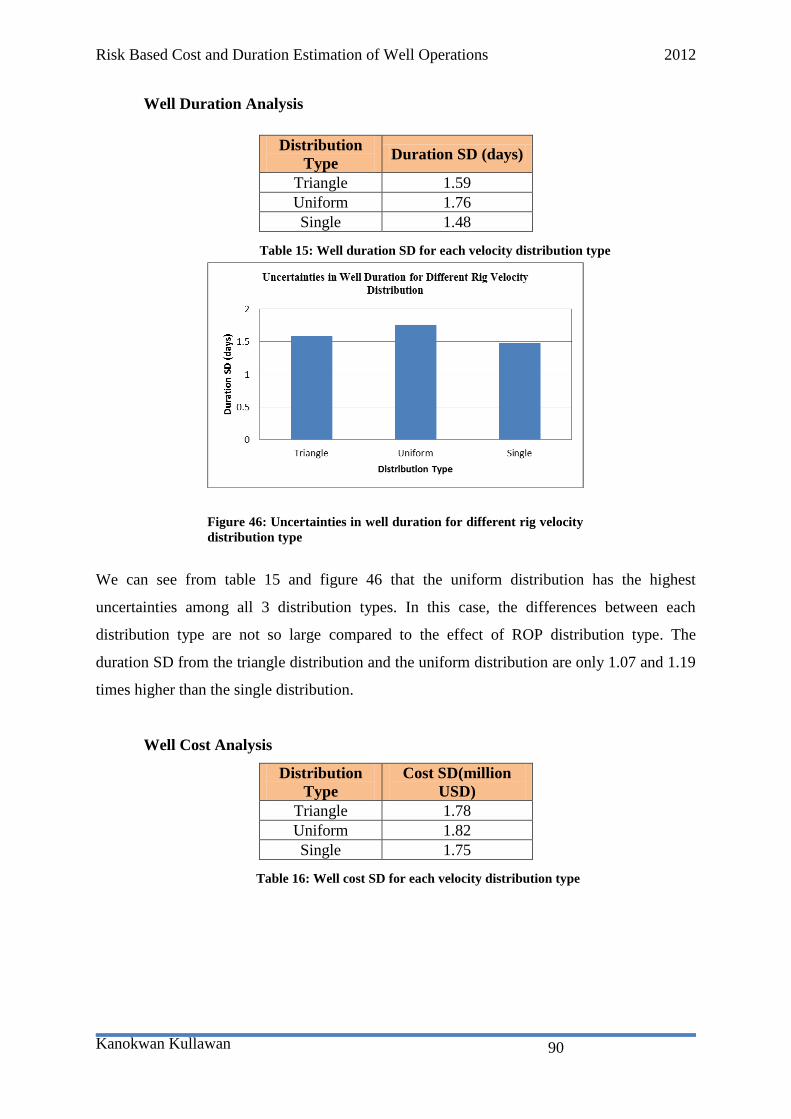
Risk Based Cost and Duration Estimation of Well Operations 2012
Kanokwan Kullawan
90
Well Duration Analysis
Distribution
Type Duration SD (days)
Triangle 1.59
Uniform 1.76
Single 1.48
Table 15: Well duration SD for each velocity distribution type
We can see from table 15 and figure 46 that the uniform distribution has the highest
uncertainties among all 3 distribution types. In this case, the differences between each
distribution type are not so large compared to the effect of ROP distribution type. The
duration SD from the triangle distribution and the uniform distribution are only 1.07 and 1.19
times higher than the single distribution.
Well Cost Analysis
Distribution
Type
Cost SD(million
USD)
Triangle 1.78
Uniform 1.82
Single 1.75
Table 16: Well cost SD for each velocity distribution type
Figure 46: Uncertainties in well duration for different rig velocity
distribution type

Risk Based Cost and Duration Estimation of Well Operations 2012
Kanokwan Kullawan
91
Figure 47 shows that the results from all 3 distribution types are pretty close to each other.
Even though the uniform distribution and the single distribution still have the highest and the
lowest uncertainties, the difference between each distribution type is insignificant.
The results from the well duration and well cost analysis demonstrate that the distribution
type of the rig moving velocity has a noticeable effect on the uncertainties of the well
duration but less significant impact on the well cost.
Value Analysis
In order to see the effect of the rig velocity on the expected value, the rig velocity input will
be varied using the single distribution. The velocity to be studied ranges from 1 nmi/hr to 9
nmi/hr.
Well Duration Analysis
Rig
Velocity(nmi/hr) Expected Duration (days)
1 33.15
3 29.82
5 29.14
7 28.87
9 28.71
Table 17: Expected duration for each rig velocity
Figure 47: Uncertainties in well cost for different rig velocity
distribution type

Risk Based Cost and Duration Estimation of Well Operations 2012
Kanokwan Kullawan
92
From figure 48, the results from using 3 nmi/hr to 9 nmi/hr are pretty close to each other. The
largest difference of the expected duration is 1.11 days when comparing using 3 nmi/hr and 9
nmi/hr rig velocity. Nevertheless, when the rig velocity is set as 1 nmi/hr, the expected
duration is obviously longer than other cases, 3.33 days extended compared to using 3
nmi/hr.
Well Cost Analysis
Rig Moving
Velocity(nmi/hr)
Expected Cost(million
USD)
1 32.25
3 29.95
5 29.48
7 29.31
9 29.22
Table 18: Expected cost for each rig velocity
Figure 48: Expected well duration for different rig velocity

Risk Based Cost and Duration Estimation of Well Operations 2012
Kanokwan Kullawan
93
Figure 49 shows that the result agrees with the well duration analysis. The velocity of the rig
move does not have a huge effect on the expected well cost except when the velocity is
extremely slow, 1 nmi/hr in this case. The expected well cost if the rig moves with 3 nmi/hr is
0.73 million USD higher than if the rig moves with 9 nmi/hr while the difference between 3
nmi/hr case and 1 nmi/hr case is 2.3 million USD.
Figure 49: Expected well cost for different rig velocities

Risk Based Cost and Duration Estimation of Well Operations 2012
Kanokwan Kullawan
94
6.5 Results from Risked Operation Plan
6.5.1 Input of Risk Events into the Well Model
In the previous section, the results from the standard operation plan have been discussed.
Now the risked operation plan will be considered by including undesirable events into the
well model. Some example of risks available in the simulator, both for the well level and the
phase level, has been identified in chapter 5. In spite of that, 4 main risk events have been
selected to be studied here which are Wait on Weather (WOW), Kick, BHA failure and Stuck
pipe.
Wait on Weather (WOW) – It is one of the most common causes of operation delays
especially in the North Sea area. Some operators have included an extra duration of 10% -
15% of the standard operation plan for WOW issue while planning the well. According to the
result of the standard operation plan, the expected duration is 29.78 days. Thus, 10% of this
duration, approximately 3 days, will be used as an input for WOW. A.J. Adams[10]
has
suggested that the Weibull distribution should be used for WOW event.
Kick/ Well Control Event – The probability of kick event can vary considerably, depending
on the activity and the geological condition. As it is mentioned in the background of the base
case well, this example well is drilled in an offshore area of the North Sea. J.D. Dobson[44]
has presented some statistical studies regarding the kick events according to the geological
basin and the rig type. When the kicks are analysed by rig type, the kicks happened least
frequently on the wells drilled by the semi-submersible rig (68 out of 333 kick events). Based
on 2,757 wells drilled in several areas of the North Sea, there are 332 kick events. As a
consequence, a kick probability of 12% will be used in this simulation.
BHA Failure – In case of BHA failure, the extra duration required depends significantly on
the depth of failure while the tripping speed is almost the same for every section. Hence, each
hole section would have different range of extra duration input.
Stuck Pipe – J.A. Howard[45]
has performed a study about stuck pipe events using a database

Risk Based Cost and Duration Estimation of Well Operations 2012
Kanokwan Kullawan
95
with data from more than 1,000 wells drilled in the Gulf of Mexico and the North Sea.
Statistically, the data showed that one of three wells drilled in the Gulf of Mexico and the
North Sea has experienced stuck pipe problems. Thus, the input probability of the event
occurrence will be set as 33%. In this case, the simulation is performed with the assumption
that the pipe can be released and there’s no extra cost due to having a BHA lost in the hole.
The table below shows the probability of occurrence and the extra duration of each risk event.
Event
Distribution
Type Probability(%) Extra Duration(hr)
Wait on Weather (WOW) Weibull 90 Scale = 72 hr, Shape = 1
Kick Triangle 12 Min = 6 hr, Peak = 12 hr, Max = 96 hr
BHA Failure 26.00" section Uniform 20 Min = 8 hr, Max = 14 hr
BHA Failure 12.25" section Uniform 20 Min = 16 hr, Max = 26 hr
BHA Failure 8.50" section Uniform 20 Min = 17 hr, Max = 28 hr
BHA Failure 6.00" section
(pilot) Uniform 20 Min = 19 hr, Max = 32 hr
BHA Failure 6.00" section(ST) Uniform 20 Min = 19 hr, Max = 32 hr
Stuck Pipe Uniform 33 Min = 4 hr, Max = 72 hr
Table 19: Input parameters for risk events
In table 19, WOW is a risk event in the well level while the rests are the events on phase
level.

Risk Based Cost and Duration Estimation of Well Operations 2012
Kanokwan Kullawan
96
6.5.2 Results of Risked Operation Plan
Figure 50 presents the results of the risk operation plan. When undesirable events are
included in the well model, the expected well duration is 36.97 days with 4.17 days standard
deviation. The duration can last from 27.18 days to 66.64 days. The expected well cost is
36.08 million USD with 3.77 million USD standard deviation. The range of possible well
cost is 25.71 million USD to 65.79 million USD. The probability of finishing the well within
the expected duration and budget is 54.7% and 54.3% respectively.
Figure 50: Well summary results of risked operatoin plan
Figure 51: Events sensitivity analysis

Risk Based Cost and Duration Estimation of Well Operations 2012
Kanokwan Kullawan
97
As the events sensitivity analysis is performed, waiting on weather (WOW) shows the
greatest effect on the well cost and duration. Its impact is apparently higher than any other
risk events included in the model as it represents 6% of the total cost and 7% of the total
duration.
6.5.3 Comparison of Results between Standard Operation Plan and
Risk Operation Plan
Well Duration(days)
Standard Operation
Plan
Risk Operation
Plan
Minimum 25.89 27.18
Mean 29.98 36.97
Maximum 38.23 66.64
SD 1.59 4.17
Well Cost(million USD)
Standard Operation
Plan
Risk Operation
Plan
Minimum 24.66 25.71
Mean 30.06 36.08
Maximum 38.74 65.79
SD 1.78 3.77
Table 20: Comparison of standard operation plan and risk operation plan
From figure 52 and table 20, the results of both standard operation plan and risk operation
plan have been compared. Figure 52 shows that histograms of well cost and duration from the
risk operation plan skewed to the right with much longer tail, compared to the standard
Figure 52: Results comparison between standard operation plan and risk operation plan

Risk Based Cost and Duration Estimation of Well Operations 2012
Kanokwan Kullawan
98
operation plan. From table 20, one can notice that the minimum estimated well cost and
duration from both plans are pretty close to each other. At the same time, the expected
duration and the expected cost of the risk operation plan is higher than the standard operation
plan i.e. 23.3% and 20.0% respectively. The most noticeable changes are the maximum
possible outcomes where the risk operation plan gives much higher values. These drive the
standard deviation of the risk operation plan to be 2.62 and 2.12 times higher than the
standard operation plan for the estimated duration and cost respectively.
In the next section, the effect of each undesirable event on the total cost and duration will be
studied.
6.5.4 Detailed Sensitivity Analysis of Undesirable Events
Figure 51 shows the sensitivity analysis of all the undesirable events included in the well
model. In this section, detailed sensitivity analysis of these events will be performed by
setting the probability of occurrence, event by event, to be zero. After that, the estimated
results will be compared with the standard operation plan and the normal risk operation plan.
The figures below show the results of risk operation plan without WOW, kick incident, BHA
failure incident and stuck pipe incident respectively.
Figure 53: Result of risk operation plan without WOW event
Figure 54: Result of risk operation plan without kick event

Risk Based Cost and Duration Estimation of Well Operations 2012
Kanokwan Kullawan
99
Figure 55: Result of risk operation plan without BHA failure event
Figure 56: Result of risk operation plan without stuck pipe event
Uncertainties Analysis
Well Duration Analysis
Operation Plan Duration SD
(days)
Standard 1.59
Risk 4.17
Risk W/O WOW 2.92
Risk W/O Kick 4.03
Risk W/O BHA failure 4.04
Risk W/O Stuck pipe 3.73
Table 21: Well duration SD for different operation plan

Risk Based Cost and Duration Estimation of Well Operations 2012
Kanokwan Kullawan
100
From table 21 and figure 57, the SD of standard operation plan is apparently lower than the
SD of other risk operation plans. When each risk event is excluded from the model one at a
time, the duration SD of each scenario is plotted against other cases. One can notice that
when WOW is excluded from the model, the duration SD reduces significantly from the
normal risk operation plan. The reasons behind could be the Weibull distribution used for
WOW event. The long tail of this distribution may drive the maximum duration to be much
longer. Thus, the well model without WOW event has a greatly reduction in duration
uncertainty compare to other risk operation plan. While the uncertainties of the risk operation
plan without kick incident and without BHA failure incident are relatively close to the normal
risk operation plan, the risk operation plan without stuck pipe incident shows slightly lower
uncertainty.
Well Cost Analysis
Operation Plan Cost SD (million
USD)
Standard 1.78
Risk 3.77
Risk W/O WOW 2.90
Risk W/O Kick 3.59
Risk W/O BHA failure 3.64
Risk W/O Stuck pipe 3.44
Table 22: Well cost SD for different operation plan
Figure 57: Uncertainties in well duration for different operation
plan
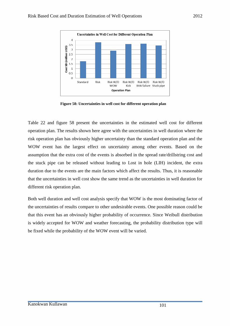
Risk Based Cost and Duration Estimation of Well Operations 2012
Kanokwan Kullawan
101
Table 22 and figure 58 present the uncertainties in the estimated well cost for different
operation plan. The results shown here agree with the uncertainties in well duration where the
risk operation plan has obviously higher uncertainty than the standard operation plan and the
WOW event has the largest effect on uncertainty among other events. Based on the
assumption that the extra cost of the events is absorbed in the spread rate/drillstring cost and
the stuck pipe can be released without leading to Lost in hole (LIH) incident, the extra
duration due to the events are the main factors which affect the results. Thus, it is reasonable
that the uncertainties in well cost show the same trend as the uncertainties in well duration for
different risk operation plan.
Both well duration and well cost analysis specify that WOW is the most dominating factor of
the uncertainties of results compare to other undesirable events. One possible reason could be
that this event has an obviously higher probability of occurrence. Since Weibull distribution
is widely accepted for WOW and weather forecasting, the probability distribution type will
be fixed while the probability of the WOW event will be varied.
Figure 58: Uncertainties in well cost for different operation plan
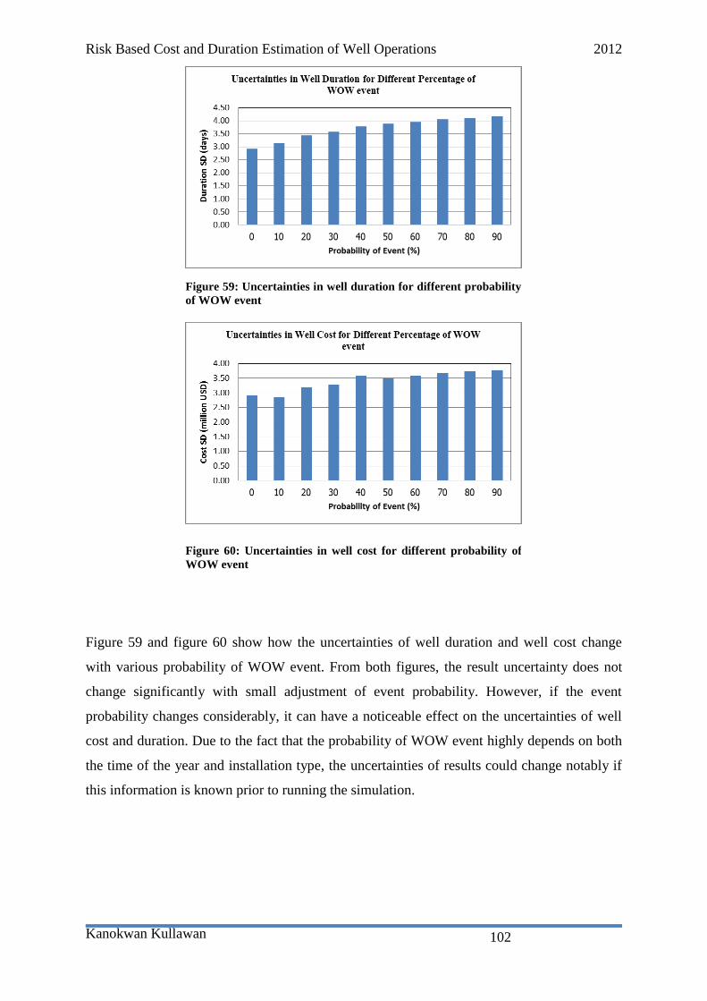
Risk Based Cost and Duration Estimation of Well Operations 2012
Kanokwan Kullawan
102
Figure 59 and figure 60 show how the uncertainties of well duration and well cost change
with various probability of WOW event. From both figures, the result uncertainty does not
change significantly with small adjustment of event probability. However, if the event
probability changes considerably, it can have a noticeable effect on the uncertainties of well
cost and duration. Due to the fact that the probability of WOW event highly depends on both
the time of the year and installation type, the uncertainties of results could change notably if
this information is known prior to running the simulation.
Figure 59: Uncertainties in well duration for different probability
of WOW event
Figure 60: Uncertainties in well cost for different probability of
WOW event
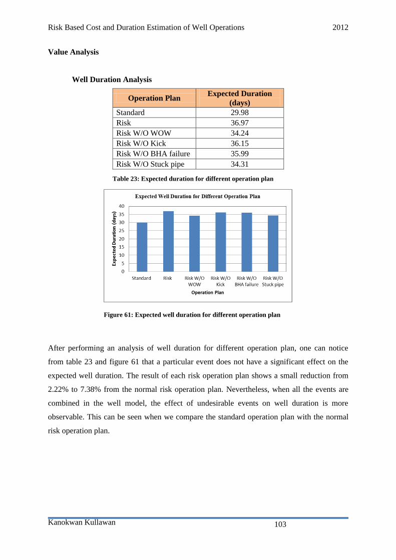
Risk Based Cost and Duration Estimation of Well Operations 2012
Kanokwan Kullawan
103
Value Analysis
Well Duration Analysis
Operation Plan Expected Duration
(days)
Standard 29.98
Risk 36.97
Risk W/O WOW 34.24
Risk W/O Kick 36.15
Risk W/O BHA failure 35.99
Risk W/O Stuck pipe 34.31
Table 23: Expected duration for different operation plan
After performing an analysis of well duration for different operation plan, one can notice
from table 23 and figure 61 that a particular event does not have a significant effect on the
expected well duration. The result of each risk operation plan shows a small reduction from
2.22% to 7.38% from the normal risk operation plan. Nevertheless, when all the events are
combined in the well model, the effect of undesirable events on well duration is more
observable. This can be seen when we compare the standard operation plan with the normal
risk operation plan.
Figure 61: Expected well duration for different operation plan

Risk Based Cost and Duration Estimation of Well Operations 2012
Kanokwan Kullawan
104
Well Cost Analysis
Operation Plan Expected Cost(million
USD)
Standard 30.06
Risk 36.08
Risk W/O WOW 34.10
Risk W/O Kick 35.26
Risk W/O BHA failure 35.19
Risk W/O Stuck pipe 33.80
Table 24: Expected Cost for different operation plan
The results of the well cost analysis shown in table 24 and figure 62 correspond to the results
of the well duration analysis. One specific event excluded from the model leads to a minute
decrease in the expected well cost from the normal risk operation plan, from 2.33% to 6.32%.
Figure 62: Expected well cost for different operation plan

Risk Based Cost and Duration Estimation of Well Operations 2012
Kanokwan Kullawan
105
7. Conclusions and Recommendations
This study focused on performing probabilistic well cost estimation and studying the
characteristics of results from an example well. Sensitivity analysis of the results has been
conducted to observe how the uncertainties and the value of the results will behave when the
input parameters are varied. Furthermore, the research also aimed to identify potential
development for the Risk€ software.
7.1 Why Probabilistic Cost Estimation
Historically, well cost estimation had been performed by a deterministic method which is
simple and easy to communicate. However, that approach turned to be too optimistic and did
not reflect the range of possible outcomes. Hence, a probabilistic approach has been
developed and its application in predicting well cost and duration has become accepted
widely in the oil and gas industry. With this method, sensitivity analysis and risk assessment
can be performed. Engineers, decision makers and stakeholders can have better knowledge
regarding the expected outcome and uncertainties in well construction processes. Thus, this
leads to better decision making process, more effective allocation of resources and an
improvement in planning to prevent time and cost overrun.

Risk Based Cost and Duration Estimation of Well Operations 2012
Kanokwan Kullawan
106
7.2 Conclusions from an Example Well
A case example well was created with an inspiration from a Statoil well program. However,
input information, especially cost related data, were estimated based on various sources
which are expert comments, literatures, personal experiences, etc. Then, a standard operation
plan was generated. Both well cost and well duration histograms showed similar shape,
which were asymmetric and skewed to the right. When the cost was broken down into cost
codes, it confirmed that time spent on well operations were obviously the most significant
contribution to the well total cost.
Phase sensitivity analysis demonstrated that drilling phase and mobilization phase were the
most dominating phases with respect to the total results. Deeper details were revealed in
operation sensitivity analysis where it was seen that drilling operation was the most
influential operation within the drilling phase and moving rig to location had the highest
impact on the mobilization phase. As a consequence, rate of penetration (ROP) and rig
moving velocity were selected for detailed sensitivity analysis.
To analyse the uncertainties, probability distribution type of both parameters was varied and
the standard deviation (SD) of the results between each distribution type was compared. The
results showed that, among 3 distribution types, the uniform distribution gave the highest
uncertainties results and the single distribution gave the lowest uncertainties results. From the
discussion in the last chapter, we may conclude that ROP was a significant uncertainty driver
and a better knowledge of an expected range of ROP could reduce the uncertainties of the
results considerably. Exact knowledge of rig moving velocity could moderately reduce the
uncertainties of results, but the impact was much less than the ROP.
In order to examine the effect of ROP on the value of the results, the expected value from 4
cases of different penetration rate were plotted against each other. The first case was base
case of the example well while the other 3 cases were the results when the ROP was set at the
minimum, most likely and maximum of the base case ROP. The results from the “Most
Likely” case were relatively close to the base case, slightly lower. This was the same
behaviour seen when comparing the deterministic and probabilistic approach. In this analysis,
the minimum and the maximum ROP were symmetric compared to the most likely value.
However, the simulation results showed asymmetric characteristics. The maximum ROP
moderately lowered the expected cost and duration to a certain level while the minimum ROP
enormously exaggerated the expected results. This behaviour was confirmed by the value
analysis of the varied rig moving velocity. When the rig velocity was varied, the expected

Risk Based Cost and Duration Estimation of Well Operations 2012
Kanokwan Kullawan
107
cost and duration remained steady except for the case of the slowest rig velocity. If the rig
moved extremely slowly, it caused a much longer delay compared to the time it could save
when moving fast. This could be due to the fact that, when the operation was very slow, that
operation would have a higher proportion of the total estimation. Thus, it led to a much
greater expected results. On the contrary, when the operation was much faster, that operation
had less impact on the estimated results and other operations would contribute more. That’s
why it did not lead to a huge decline in the expected results.
After performing detailed sensitivity analysis of the standard operation plan, 4 major risk
events were included into the simulation and the risk operation plan was generated. When
comparing the results from the standard operation plan and the risk operation plan, the latter
had much greater dispersed data. This led to much higher standard deviation and
exceptionally longer tail on histogram charts for both cost and duration. The effect of each
event on the total duration was examined by excluding the event from the simulation one at a
time. According to the event sensitivity analysis, wait on weather (WOW) demonstrated the
greatest impact among all the risks. The uncertainties of results dropped significantly when it
was excluded from the simulation as well. On the other hand, the kick event and the BHA
failure event showed a negligible change when they were excluded from the simulation.
WOW was examined if its high probability of occurrence was the key driver of the results.
Then, it was found out that if the probability of WOW event changed significantly, a
noticeable decrease in uncertainties could be expected. Hence, knowing the time of the year
that the operations would take place and the installation type that would be used could lead to
more accurate results.
Even though the risk events were responsible for huge increase in uncertainties, the impact on
the expected values were not that obvious. There was no particular event that clearly
influenced the expected results. Excluding each risk event from the simulation only showed a
small reduction from the normal risk operation plan.
It was mentioned before that time spent on well operations had a huge impact on the
estimated cost and time-based cost had a large proportion of the total cost. This was
confirmed by the study where all the cost analysis showed the same trend as the duration
analysis. The only difference was that the magnitude of change in the well cost was slightly
smaller than in the well duration. This was reasonable since the cost was also contributed
from the fixed cost which would not change with the changing duration.

Risk Based Cost and Duration Estimation of Well Operations 2012
Kanokwan Kullawan
108
7.3 Recommendations for Future Study and Software
Development
One goal of this study is to identify the potential improvements of the Risk€ software to
enhance the efficiency of future study. During the research, there are some ideas which I
think could be appealing to appraise more thoroughly if these could be developed in the
future version of the Risk€ software. The suggestions are from the literature review,
simulation and analysis process and personal experience as a software user. These
recommendations are divided into 2 categories. The first one is the suggestion for the
software to expand its function and be able to handle more well operations situations. The
second one is the opinion about how the software could be improved to be friendlier to the
user.
7.3.1 Software Development to Cover More Well Operations
Situations
In the example well consideration, the well was designed to drill a 6” pilot hole prior to
plugging back and sidetrack the well. However, the well architecture cannot handle this
situation. The sidetrack section cannot be represented in the well schematic and the
software treats the sidetrack section as the deeper section from the 6” pilot section. I
would like to propose that Risk€ should be extended to set up the well architecture for a
multilateral well.
When dealing with the stuck pipe event, the user can add extra duration and extra cost
associated with the event. In spite of that, the software does not provide an option to
separate between the cases where the pipe can be released and the lost in hole (LIH)
situation. In case of LIH, a huge extra cost due to BHA would occur. Besides, the well
will need to be plugged back and sidetrack. These costs cannot be simply added as an
extra cost of the stuck pipe event; otherwise, it will be directly treated as the cost of the
event no matter the pipe can be released or not. Thus, I would recommend that the
software will be able to deal with “what-if” scenario and the results from each case could
be compared. A similar situation can occur for a kick event. If the kick event evolves into
a blowout, the consequences will be much more devastating in terms of operations cost
and duration.
One common decision to be made during drilling is if the bit becomes dull, where the

Risk Based Cost and Duration Estimation of Well Operations 2012
Kanokwan Kullawan
109
decision is between continue drilling with the same bit and encounter slower ROP or trip
out of hole to change the bit. In order to compare these 2 scenarios, it would be
convenient for the users if the different range of expected ROP can be selected in one
section. The expected range of ROP can have a huge difference between drilling with the
new bit and the worn bit.
As mentioned earlier, this simulation tool divides the drilling operations into phases and
it works with one well at a time. This is more suitable for an exploration well. For the
field development campaign, batch drilling technique can be used. It would be great if
the software is extended to support this technique.
While working with batch drilling, it is believed that the work efficiency tends to
improve and less time will be required for the same operation. Thus, if the software is
extended to support batch drilling technique, the learning curve effect should also be
included.
While planning the well, not only the cost of drilling operations, but the cost due to
running completion processes is also an important concern. Broadening the software
features to cover the completion processes would be a great benefit for both the
engineers who write the AFE and the decision makers.
For future study, once the software is developed to cover these cases, it would be interesting
to perform well cost and duration estimation for these scenarios. It could also be appealing
for Risk€ to have a potential for analysing new drilling technologies compared to the
conventional approach. New technology is likely to be more expensive with lack of
historical data but may lead to better efficiency operation while the conventional method is
more predictable. A risked base approach could be appropriate for analysing this.
7.3.2 Software Development to Enhance Efficiency in Simulation
Process
In the distribution mode input panel, the user can select either the common distribution;
such as single value distribution, discrete distribution, uniform distribution, triangle
distribution, piecewise linear distribution, or the advanced distribution; such as generic
distribution, normal distribution, exponential distribution, Weibull distribution, is more
appropriate for that parameter. Nevertheless, for some parameter such as ROP, the
Risk Based Cost and Duration Estimation of Well Operations 2012
Kanokwan Kullawan
110
advanced distributions are disabled and cannot be selected.
One advantage of the software is that several alternatives can be compared with each
other. It would strengthen this advantage if there is an option to copy alternative.
Sometimes, the alternatives to be compared may be different in only few phases or
operations and the rests of the well model are the same. Thus, it would be much faster to
compare many alternatives when the users only need to work with the processes of
interest and no need to create the whole well again. This idea also applies with phase and
operations. It should be possible to copy them such that the user only needs to change the
necessary inputs.
The normal distribution may be appropriate with many input parameters. However, it
might not be chosen for the simulation since its tail could give an unreasonable value.
For example, it may give a negative value which is not sensible for many parameters.
Thus, it would be advantageous if the user can set the boundary (cut off) for the normal
distribution in the software.
Risk Based Cost and Duration Estimation of Well Operations 2012
Kanokwan Kullawan
111
References
1. Global Petroleum Consulting & Trading Limited: http://gpcpetro.com/. 30Mar2012.
2. http://www.drillingformulas.com/mobile-formation-causes-stuck-pipe/. 15Mar2012.
3. Oil&Gas Financial Journal: http://www.ogfj.com/articles/print/volume-8/issue-
12/features/who-moved-my-rig.html. 13Apr2012.
4. Boost C++ Libraries:
http://www.boost.org/doc/libs/1_35_0/libs/math/doc/sf_and_dist/html/math_toolkit/di
st/dist_ref/dists/weibull.html. 06Mar2012.
5. United States Department of Labor - Occupational Safety & Health Administration:
http://www.osha.gov/SLTC/etools/oilandgas/drilling/kickback_final.html. 15Mar2012.
6. H.Begg, R.B.B.a.S., Making Good Decisions. First ed2010, United States of America:
Society of Petroleum Engineers.
7. Loberg, T., et al., The How's and Why's of Probabilistic Well Cost Estimation, in
IADC/SPE Asia Pacific Drilling Technology Conference and Exhibition2008, 2008,
IADC/SPE Asia Pacific Drilling Technology Conference and Exhibition: Jakarta,
Indonesia.
8. Petroleum Online IHRDC e-Learning Solutions:
http://www.petroleumonline.com/content/overview.asp?mod=4. 10Feb2012.
9. AMAR, R., Drilling Performance Management System, in International Petroleum
Technology Conference2007, International Petroleum Technology Conference: Dubai,
U.A.E.
10. Adams, A., C. Gibson, and R.G. Smith, Probabilistic Well-Time Estimation Revisited.
SPE Drilling & Completion, 2010(12).
11. Saibi, M., A Probabilistic Approach for Drilling Cost Engineering and Management
Case Study: Hassi-Messaoud Oil Field, in SPE/IADC Middle East Drilling and
Technology Conference2007, 2007, SPE/IADC Middle East Drilling Technology
Conference & Exhibition: Cairo, Egypt.
12. Schlumberger Oilfield Glossary: http://www.glossary.oilfield.slb.com. 03Mar2012.
13. Peterson, S.K., J.A. Murtha, and F.F. Schneider, Risk Analysis and Monte Carlo
Simulation Applied to the Generation of Drilling AFE Estimates, in SPE Annual
Technical Conference and Exhibition1993, 1993 Copyright 1993, Society of
Petroleum Engineers, Inc.: Houston, Texas.
14. Hariharan, P.R., R.A. Judge, and D.M. Nguyen, The Use of Probabilistic Analysis for
Estimation of Drilling Time and Costs When Evaluating Economic Benefits of New
Technologies, in IADC/SPE Drilling Conference2006, Society of Petroleum
Engineers: Miami, Florida, USA.
15. Kitchel, B.G., et al., Probabilistic Drilling-Cost Estimating. SPE Computer
Applications, 1997(07-08).
16. Chen, M. and J. Dyer, Inevitable Disappointment in Projects Selected on the Basis of
Forecasts. SPE Journal, 2009. 14(2): p. pp. 216-221.
17. Akins, W.M., M.P. Abell, and E.M. Diggins, Enhancing Drilling Risk & Performance
Management Through the Use of Probabilistic Time & Cost Estimating, in SPE/IADC
Drilling Conference2005, SPE/IADC Drilling Conference: Amsterdam, Netherlands.
18. International Research Institute of Stavanger: http://www.iris.no/Internet/energy.nsf/.
02Apr2012.
19. Palisade Corporation Website: http://www.palisade.com/risk/. 06Mar2012.
20. Oracle: http://www.oracle.com/us/products/applications/crystalball/index.html.
06Mar2012.

Risk Based Cost and Duration Estimation of Well Operations 2012
Kanokwan Kullawan
112
21. Hollund, K.U., et al., Hitting Bull's-Eye with Time and Cost Estimates by Combining
Statistics and Engineering, in SPE Annual Technical Conference and Exhibition2010,
Society of Petroleum Engineers: Florence, Italy.
22. Halliburton Products & Services:
http://www.halliburton.com/ps/default.aspx?pageid=1515&navid=217&prodid=PRN
::JI3EXQ15. 06Mar2012.
23.
http://www.slb.com/~/media/Files/drilling/industry_articles/200707_ep_plann
ing.ashx. 12Mar2012.
24. Zoller, S.L., J.-R. Graulier, and A.W. Paterson, How Probabilistic Methods Were
Used to Generate Accurate Campaign Costs for Enterprise's Bijupirá & Salema
Development, in SPE/IADC Drilling Conference2003, SPE/IADC Drilling
Conference: Amsterdam, Netherlands.
25. Capen, E.C., The Difficulty of Assessing Uncertainty (includes associated papers
6422 and 6423 and 6424 and 6425 ). SPE Journal of Petroleum Technology,
1976(08).
26. Jablonowski, C., et al., Integrating Learning Curves in Probabilistic Well-
Construction Estimates. SPE Drilling & Completion, 2011(03).
27. Brett, J.F. and K.K. Millheim, The Drilling Performance Curve: A Yardstick for
Judging Drilling Performance, in SPE Annual Technical Conference and
Exhibition1986, 1986 Copyright 1986, Society of Petroleum Engineers: New Orleans,
Louisiana.
28. Everitt, B.S., The Cambridge Dictionary of Statistics. Second ed2002, United States
of America: Cambridge University Press.
29. Schuyler, P.D.N.a.J., Decision Aalysis for Petroleum Exploration. Second ed2000:
Planning Pr.
30. Murtha, J.A., Monte Carlo Simulation: Its Status and Future. SPE Journal of
Petroleum Technology, 1997(04).
31. Williamson, H.S., S.J. Sawaryn, and J.W. Morrison, Monte Carlo Techniques Applied
to Well Forecasting: Some Pitfalls. SPE Drilling & Completion, 2006(09).
32. A. Saltelli, K.C., E.M. Scott, Sensitivity Analysis2001, United Kingdom: John Wiley
& Sons Ltd.
33. William C. Lyons, P., P.E., Standard Handbook of Petroleum & Natural Gas
Engineering. Vol. 1. 1996, United States of America: Gulf Publishing Company.
34. Inglis, T.A., Petroleum Engineering and Development Studies. Vol. 2 - Directional
Drilling. 1987, United Kingdom: Graham &Trotman Limited.
35. Turrentine, R.E., G.W. Huff, and G.F. Oglesby, Analysis of Drilling Ship
Performance, in Offshore Technology Conference1973: Houston, Texas.
36. Mitchell, R.F. and M.B. Allen, Case Studies of BHA Vibration Failure, in SPE
Annual Technical Conference and Exhibition1987, 1987 Copyright 1987, Society of
Petroleum Engineers: Dallas, Texas.
37. Bernt S. Aadnoy, I.C., Stefan Z. Miska, Robert F. Mitchell, and Michael L. Payne,
Advanced Drilling and Well Technology. First ed2009, United States of America:
Society of Petroleum Engineers.
38. Drilling Specialties Company - Technical Library:
http://www.cpchem.com/bl/drilling/en-us/Pages/DrillingMudsLiterature.aspx.
30Mar2012.
39. Jr., A.T.B., Applied Drilling Engineering. First ed1986, United States of America:
Society of Petroleum Engineers.
40. Marken, C., S. Hansen, and J. Øregaard, Shallow Gas Kick: Simulation and Analysis
Risk Based Cost and Duration Estimation of Well Operations 2012
Kanokwan Kullawan
113
for Top Hole Drilling Without a Riser, in SPE Annual Technical Conference and
Exhibition2000, Copyright 2000, Society of Petroleum Engineers Inc.: Dallas, Texas.
41. Adams, N.J. and L.G. Kuhlman, Case History Analyses of Shallow Gas Blowouts, in
SPE/IADC Drilling Conference1990, 1990 Copyright 1990, IADC/SPE Drilling
Conference.: Houston, Texas.
42. T. Løberg, E.P.F.a.B.D., Risk€ Software User Manual.
43. Risk€ Library.
44. Dobson, J.D., Kicks in Offshore UK Wells�Where Are They Happening, And
Why?, in SPE/IADC Drilling Conference and Exhibition2009, British Crown
Copyright: Amsterdam, The Netherlands.
45. Howard, J.A. and S.B. Glover, Tracking Stuck Pipe Probability While Drilling, in
SPE/IADC Drilling Conference1994, 1994 Copyright 1994, IADC/SPE Drilling
Conference: Dallas, Texas.

Risk Based Cost and Duration Estimation of Well Operations 2012
Kanokwan Kullawan
114
Appendix A: Matlab Code
Matlab code for Monte Carlo sample calculation
o Drilling cost estimation without events.
function C = calCost(N)
ROP = trianglerand(5,20,35,100000);
%ROP in m/hr.
for i = 1:N
Length = 1000; % section length is 500m.
Rigrate(i) = unifrnd(4,7);
% Daily rig rate is in million NOKtitle
C(i) = 1000/ROP(i)*Rigrate(i)/24 + 2;
%fixed cost is 2 millionNOK.
end
N = 100000; % number of repeated trials
C = calCost(N);
hist(C,500); % 50 is number of histogram columns
mu1 = mean(C);
me1 = median(C);
sd1 = std(C);
o Drilling cost estimation with events included.

Risk Based Cost and Duration Estimation of Well Operations 2012
Kanokwan Kullawan
115
function Z = calCost2(N)
ROP = trianglerand(5,20,35,100000);
%ROP in m/hr.
Event = trianglerand(2,30,60,100000);
for i = 1:N
Length = 1000; % section length is 500m.
Rigrate(i) = unifrnd(4,7);
% Daily rig rate is in million NOK
C(i) = 1000/ROP(i)*Rigrate(i)/24 + 2;
%fixed cost is 2 millionNOK.
on = (rand<0.2);
Z(i) = C(i) + Event(i)*Rigrate(i)/24*on;
end
N = 100000; % number of repeated trials
Z = calCost2(N);
hist(Z,500); % 50 is number of histogram columns
mu2 = mean(Z);
me2 = median(Z);
sd2 = std(Z);