RISK AVERSE APPROACHES IN OPEN-PIT PRODUCTION

PLANNING UNDER ORE GRADE UNCERTAINTY: A ULTIMATE PIT

STUDY

Daniel Espinoza, daespino@dii.uchile.cl, Assistant Professor, Department of Industrial

Engineering, Universidad de Chile, Avda. Republica 701 Oficina 307, Santiago Centro,

Santiago, Chile, +56-2-2978-4036

Guido Lagos (corresponding author), glagos@gatech.edu, Ph.D. Student, H. Milton Stewart

School of Industrial & Systems Engineering, Georgia Institute of Technology, 765 Ferst Dr NW,

Atlanta, GA 30332-0205, USA, +1-412-737-8101

Eduardo Moreno, eduardo.moreno@uai.cl, Associate Professor, School of Engineering,

Universidad Adolfo Ibañez, Avda. Diagonal Las Torres 2640 Oficina 5, Peñalolen, Santiago,

Chile, +56-2-2331-1351

Juan Pablo Vielma, jvielma@mit.edu, Assistant Professor, Sloan School of Management,

Massachusetts Institute of Technology, 77 Massachusetts Ave. Room E62-561, Cambridge, MA

02139, USA, +1-617-324-1204

ABSTRACT

During early phases of open-pit mining production planning many parameters are uncertain,

and since the mining operation is performed only once, any evaluations based only on on

average outcomes neglects the very real chance of obtaining an outcome that is below average.

Taking into account also that operation costs are considerable and the mining horizon usually

extends over several decades it is clear that open-pit production planning is a risky endeavor. In

this work we take a risk-averse approach on tackling uncertainty in the ore-grades. We consider

an extended Ultimate-Pit problem, where extraction and processing decisions have to be taken.

We apply and compare the risk-hedging performance of two approaches from optimization

under uncertainty: minimize Conditional Value-at-Risk (CVaR) and minimization of a

combination of expected value and CVaR. Additionally, we compare two decision schemes: a

static variant, where all decisions have to be taken ―now‖, and a two-stage or recourse variant,

where we take extraction decisions now, then we see the real ore-grade, and just then processing

decision is taken. Our working assumption is that we have available a large number of ore-

grade scenarios. Computational results on one small size vein-type mine illustrate how

minimizing average loss provides good on-average results at the cost of having high probability

of obtaining undesired outcomes; and on the other hand our proposed approaches control the

risk by providing solutions with a controllable probability of obtaining undesired outcomes.

Results also show the great risk-hedging potential of using multi-stage decision schemes.

INTRODUCTION

The geological uncertainty of ore grades is crucial in mine planning and it has received

significant attention in the last decade. Studies have shown that incorporating the uncertainty of

the ore grades into the problem could lead to final pits 15% larger in tonnage, and adding a 10%

of value, see Dimitrakopoulos (2011). The most common tool to model this uncertainty is the

use of conditional simulations of orebodies, see e.g. Dimitrakopoulos (1998) and Benndorf and

Dimitrakopoulos (2004). For instance Dimitrakopoulos et al. (2007) use conditional simulations

to obtain candidate plans based on several orebody models, and Whittle and Bozorgebrahimi

(2004) use conditional simulations to generate so-called Hybrid Pits based on set-theory.

Marcotte and Caron (2012) estimate the maximum expected value of mine when extraction

decisions rely on uncertain information but by the time of processing all information is known.

A characteristic of these approaches is that they aim to optimize the expected profit of the

operation, an eminently risk-neutral approach; however this may be inconvenient in situations

where the operation is not being repeated continuously under similar conditions –contrast with

operations in airline industry–, moreover when losses at stake are considerable. In view of this,

and in an attempt to directly include risk control into the optimization model, Vielma et al.

(2009) proposed a chance-constrained model that looks for solutions with low probability of

obtaining low profits. The work we present here is a follow up on the latter one and builds upon

its idea of using an optimization process which directly assesses the risk of feasible solutions.

In this paper we propose several risk-averse optimization methods that take into account the

uncertainty in the ore-grade parameter. Our basic working assumption is that we have access to

a pool of independent and identically distributed joint ore-grade vectors. The main advantage of

this approach is that in this way we separate the optimization model from the geo-statistical

technique that models the mineralization of the orebody. We work on the Ultimate-Pit problem,

since it is a simple yet relevant aspect of life of mine planning, and consider an extended

version where extraction and processing decisions have to be taken. We present and apply two

risk-averse optimization approaches whose theoretical properties have been well studied, and

also propose a two-stage decision scheme where after extraction occurs we can see the true

mineralization of the extracted blocks. We show computational results on a small size vein-type

mine and exhibit the practical strengths and weaknesses of the proposed models.

The rest of this text is organized as follows. In Section 2 we present the extended Ultimate-Pit

problem on which we work. In Section 3 we introduce two decision paradigms available for the

problem, and illustrate their differences by two opposite optimization models in terms of risk.

In Section 4 we describe the two risk-averse optimization approaches we propose to use for the

UPIT problem, and go through their most important properties in the theory of risk-averse

optimization. In Section 5 we show computational results made on a small size mine and show

the performance of our proposed method. Lastly, in Section 6 we state the conclusions of our

work.

THE ULTIMATE-PIT PROBLEM

The Ultimate-Pit problem (UPIT), also known as uncapacited open-pit mine planning problem,

consists in finding the set of blocks which should be ultimately extracted, in the absence of

capacity constraints, in order to maximize the value of the mine. Despite its simplicity, UPIT is

a key problem for mine planning. In Caccetta and Hill (2003) they prove that the optimal multi-

period capacitated open-pit mine planning problem is included in the solution of the UPIT.

Moreover, a series of UPIT problems are solved to construct the nested pits, see Whittle (1988),

which is the basis of the most common methodology to schedule open-pit mines.

We consider the following extended UPIT problem, where extraction as well as processing

decisions have to be made. Let B be a set of blocks, each one with an associated cost bc --a

negative cost is a profit-- for all Bb . Let BBP be a set of precedences, that is, if

Pb)(a, then in order to extract block a , block b should also be extracted. Only if it is

extracted a block can be processed, and an extracted one can be either processed or discarded.

Extraction of block b incurs a cost of e

bc ; if it is discarded it does not incur any additional cost,

but if it is processed it incurs an additional cost of bb

p

b pρc , where p

bc is the processing cost,

bρ is its mineral content or ore grade, and bp is the unitary profit for processing a unit of

mineral in it. A mathematical formulation of the UPIT optimization problem is

min e

b

e

b

p

bbb

p

b

pestat xc+)xpρ(c=ρ),x,(xL : s.t. EPpe Xx,x (1)

where

BbxxP,b)(a,xxx,x=X e

b

p

b

e

b

e

a

BpeEP :0,1:

and where binary variables e

bx and p

bx indicate if block b should be extracted (resp.

processed) or not. Of course, 1=x p

b if and only if 1=xe

b and 0<pρc bb

p

b , which allows to

decide a priori if a block will be processed if extracted; with this, one can eliminate the

processing variables in (1) and include all the processing decisions and costs in the extraction

costs, as in Marcotte and Caron (2012). We choose however to skip this preprocessing step and

build upon the formulation (1) for clarity of exposure, and also because this formulation,

applied with the risk-averse models shown hereafter, is readily extendible to other mining

models and constraints, e.g. one can include constraints on the processing decisions, include

planning over several time periods, etc.

UPIT UNDER ORE-GRADE UNCERTAINTY

Uncertainty Model for the Ore Grades

A weakness of problem (1) is that it does not account for the inherent uncertainty of the

estimated ore grade vector ρ . Indeed, the precise mineral composition in each location of the

orebody is only partially known since the only information available are exploration drillings.

To assess for this uncertainty we assume in this work that, first, the ore vector is actually a

random vector ρ~ in B

+ , and second, that we can take as many independent and identically

distributed (i.i.d.) samples of it. Note that this assumption allows modeling non-i.i.d. samples,

and also capturing correlations between different blocks. Note also that thus we are not

requiring knowledge of the actual joint distribution of the random vector ρ~ .

Static vs. Two-Stage Decision Schemes and Basic Risk Models

We first note that the following formulation is completely equivalent to (1):

min ρ),Q(x+xc=ρ),(xL ee

b

e

b

erec : s.t. Ee Xx (2)

where

=ρ),Q(xe : min

Bb

p

bbb

p

b )xpρ(c

s.t. e

b

p

b xx Bb

0,1p

bx Bb

and

.:0,1: P(a,b)xxx=X e

b

e

a

BeE

This formulation emphasizes the dependence of the processing decision on the extraction

decision. An apparently unnecessary complication of (1), both formulations in fact differ when

uncertainty is introduced. Indeed, suppose ρ is now a random vector ρ~ and we want, for

instance, to minimize the expected loss; since we are assuming only availability of an i.i.d.

sample Nρ,,ρ 1 , N as big as we want, then we can either minimize the average loss of (1):

min N

=k

kpestat )ρ,x,(xLN 1

1 s.t. ,X)x,(x EPpe (3)

or the average loss of (2):

min N

=k

kerec )ρ,(xLN 1

1 s.t.

Ee Xx (4)

both computationally tractable formulations.

Note that (3) gives an extraction and processing plan that should be used in any scenario, and in

contrast (4) gives an extraction plan to use in any scenario and a processing plan for each

scenario. Essentially, (4) uses a two-stage decision scheme where extraction decision is taken

now, then the real ore-grade is revealed, and only then processing decision needs to be taken;

and (3) uses a static decision scheme, where all decisions need to be taken now. Using the

terminology of optimization under uncertainty community, we say then that (3) is a static

approach, and (4) is a recourse approach, since in the latter we have the extra recourse of

―seeing‖ the uncertain parameter before deciding the processing decision.

We remark also that Marcotte and Caron (2012) work with the recourse scheme (4) since it is a

better approach than (3) when estimating the value of mine, under the hypothesis that at later

stages of the operation there will be better ore-grade estimates. Note that, when optimizing the

average loss, the static approach (i.e. (3)) is equivalent to just plugging-in the average ore-grade

in (1), so essentially Marcotte and Caron (2012) are comparing working with the average ore-

grade and working with profit scenarios. In contrast, we seek to compare the static decision

scheme with the recourse one under several risk-averse optimization models.

Note that minimization of average losses is essentially a risk-neutral approach, since it ignores

the distribution of below- and above-average losses. Although by design this approach is the

one that will provide the best on-average outputs, it can return solutions with high probability of

obtaining big losses. On the contrary, an extreme risk-averse approach would be to minimize de

worst possible loss. In this case we are sure that the obtained solution will do well –better than

any other solution, by design– even in the worst possible scenario. A computationally tractable

formulation, for the static and the recourse versions, is easily obtained by minimizing the

maximum-loss scenario when considering losses over a finite sample of ore-grades. We

consider then minimization of expected- and worst-loss as the two opposite benchmarks when

evaluating the performance of the risk-averse approaches presented in the following section.

RISK-AVERSE MODELS FOR UPIT UNDER UNCERTAINTY

We now introduce the two risk-averse optimization models that we compare in our work:

optimization of Conditional Value-at-Risk model and ε-Modulated Convex-Hull model. A

closely related approach to the first model is the optimization of Value-at-Risk model, in which

one optimizes the ε-quantile of the worst losses, as in Vielma et al. (2009). However, in Lagos

et al. (2011) we showed that this model returned plans with good Value-at-Risk but at the

expense of having higher chance of exhibiting bad losses. This inadequate manage of risk lastly

deems the model inappropriate for the use in large scale open-pit mining planning problems,

and such is the reason we do not include it in this study.

All the models in this section can be applied to both the static and the recourse decision

schemes, however for the sake of space economy we explain them only for the static version.

To obtain the recourse versions in all models it is sufficient to replace ρ),x,(xL pestat by

)ρ,(xL kerec , and EPpe X)x,(x by Ee Xx . All strategies and properties shown here will hold

for the recourse variant as well: we rely on the SAA approximation too for computational

tractability, we have the same risk-hedging properties, convergence of optimal value and

solution set, etc.

CVaR Model

Given a risk level ](ε 0,1 (lower ε means lower risk), and given a real random variable l~

representing losses, the Conditional Value-at-Risk (CVaR) at level ε is roughly speaking the

mean of the ε portion of the worst losses. In Rockafellar and Uryasev (2000) it is shown that

CVaR can be defined, consistently with the previous notion, in the following way:

+

zε z]lE[ε

+z=lCVaR~1

min:~

where a=[a]+ if 0>a and 0 otherwise. Theoretically, CVaR is a good measure of the risk of

the random loss l~

since it is a coherent risk measure in the sense of Artzner et al. (1999).

Moreover, it is the fundamental distortion risk measure, see e.g. Bertsimas and Brown (2009).

The first model we consider then is the minimization of CVaR, where given a risk level

](ε 0,1 we choose the plan EPpe Xx,x that minimizes ))ρ,x,(x(LCVaR pestat

ε~ . From

Rockafellar and Uryasev (2000), this optimization problem can be formulated as

min +pestat z])ρ,x,(xE[L

ε+z ~1

s.t. .EPpe X)x,(x,z (5)

This problem, as it is, is intractable since the expected value in the objective function requires

multidimensional integration and over a distribution that is unknown. Therefore we use the so-

called Sample Average Approximation (SAA), which consists of approximating the expected

value by the sample average of a finite sample of the uncertain parameter. That is, we take an

i.i.d. sample Nρ,,ρ 1 of the grades vector ρ~ and solve instead

min

N

=k

+kpestat z])ρ,x,(x[LNε

+z1

1 s.t. .EPpe X)x,(x,z (6)

This latter problem is easily linearized by including one linear variable per each scenario,

obtaining thus a tractable MILP program –which applies for both the static and the recourse

versions.

We call (5) the real CVaR problem and (6) the SAA CVaR problem. SAA approximations have

been widely studied, see e.g. Linderoth et al. (2006), and under mild assumptions (see Lagos,

2011, and §5.1.1 Shapiro et al., 2009) it holds that the SAA CVaR problem is consistent with

the real CVaR problem, in the sense that as the number N of samples increases the optimal

value and set of optimal solutions of (6) converges to the respective counterparts of (5).

MCH-ε Model

The second model we consider is the so-called ε-Modulated Convex-Hull (MCH-ε) model. This

approach is a modification of the MCH model proposed in Lagos et al. (2011), where a

modulated convex-hull of an i.i.d. sample was taken as the uncertainty set in a robust-type

formulation. Although the nice theoretical properties of this latter approach, the advantage of

MCH-ε model is that its underlying risk measure does not depend on the sample size N, and is

easily extendible to a two-stage decision scheme, as will be seen in Section 3.

Consider a risk level ](ε 0,1 . The MCH-ε model consists on choosing the plan that solves

min )ρ,x,(xLCVaRε)(+)ρ,x,(xLEε pestat

ε

pestat ~1~ s.t. EPpe X)x,(x (7)

Theoretically this model is attractive since we are minimizing a well-studied distortion risk

measure of the losses that could be a better estimator of the CVaR-ε, see Lagos et al. (2012).

Now, as in the CVaR model, this model, as it is, is intractable since it requires high dimensional

integration and knowledge of the precise distribution of the ore grades vector ρ~ . Hence we

proceed as before and use the SAA approximation to solve an approximated model: we take an

i.i.d. sample Nρ,,ρ 1 of ρ~ and approximate )ρ,x,(xLE pestat ~ and )ρ,x,(xLCVaR pestat

ε~

with the in-sample mean, to obtain the problem

min

N

=k

+kpestatN

=k

kpestat z])ρ,x,(x[LNε

+zε)(+)ρ,x,(xLN

ε11

11

1

s.t. .EPpe X)x,(x,z

(8)

This problem is easily linearized by adding one linear variable per scenario, obtaining a

tractable MILP program. As in the CVaR model, convergence, as the number of samples N

increases, of the optimal value and set of the problem (8) to the respective counterparts of the

―true‖ problem (7) is a.s. assured under mild assumptions, see Lagos (2011) and §5.1.1 Shapiro

et al. (2009).

COMPUTATIONAL EXPERIMENTS

We apply these models on a small size vein-type mine, for which an i.i.d. sample of 20,000 ore-

grades vectors are available using Emery and Lantuéjoul (2006). The mine consists of 6,630

10×10×10m3 blocks from a real orebody, and when adding a crown of zero mineral content on

the sides we obtain a total of approx. 19,700 blocks and approx. 86,450 extraction precedences.

The extraction and processing costs per block are respectively 1 and 5 monetary units, and each

mineral unit processed produces a benefit of 25 monetary units. Each experiment consists of the

following: choose one of the four models (CVaR static, MCH-ε static, CVaR recourse or MCH-

ε recourse), choose a risk level ](ε 0,1 , choose a sample size N and choose at random N ore-

grades vectors out of the 20,000 pool available; with this solve the SAA approximation of the

model, thus obtaining a candidate production plan. All MILP programs are solved with the

solver CPLEX v. 12. We also consider the models of, given an ore-grade sample, choose the

plan that minimizes the expected in-sample loss, and choose the plan that minimizes the worst

in-sample loss. Additionally, for every obtained plan we calculate the loss in each of the N

scenarios used for solving the model –we call them in-sample losses–, and also calculate the

loss in a different ore-grade sample consisting of 10,000 ore-grade scenarios out of the 20,000-

N samples left –this we call the out-of-sample losses. The idea is that the in-sample losses

provide insight of ―what the model thinks it is doing‖, and the out-of-sample losses of ―what the

model is actually doing‖.

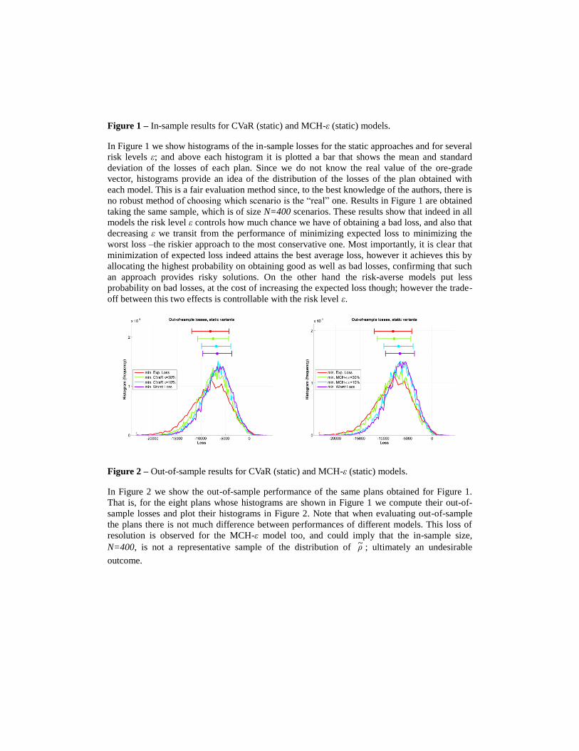
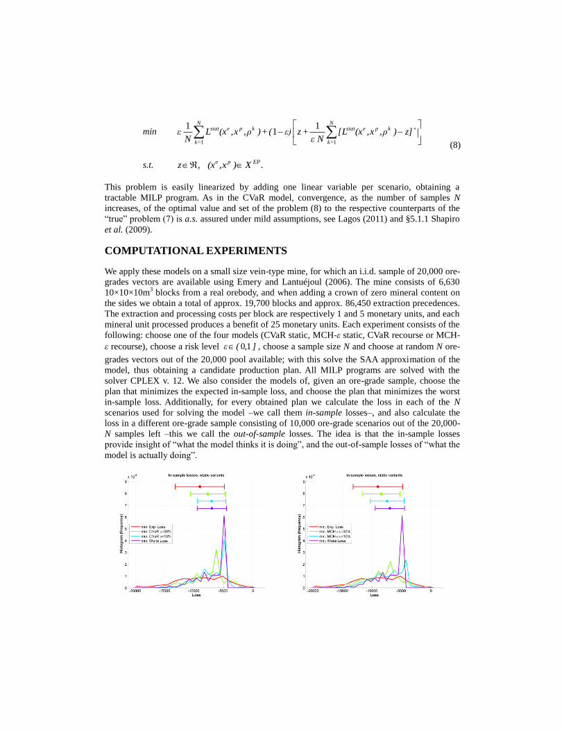
Figure 1 – In-sample results for CVaR (static) and MCH-ε (static) models.

In Figure 1 we show histograms of the in-sample losses for the static approaches and for several

risk levels ε; and above each histogram it is plotted a bar that shows the mean and standard

deviation of the losses of each plan. Since we do not know the real value of the ore-grade

vector, histograms provide an idea of the distribution of the losses of the plan obtained with

each model. This is a fair evaluation method since, to the best knowledge of the authors, there is

no robust method of choosing which scenario is the ―real‖ one. Results in Figure 1 are obtained

taking the same sample, which is of size N=400 scenarios. These results show that indeed in all

models the risk level ε controls how much chance we have of obtaining a bad loss, and also that

decreasing ε we transit from the performance of minimizing expected loss to minimizing the

worst loss –the riskier approach to the most conservative one. Most importantly, it is clear that

minimization of expected loss indeed attains the best average loss, however it achieves this by

allocating the highest probability on obtaining good as well as bad losses, confirming that such

an approach provides risky solutions. On the other hand the risk-averse models put less

probability on bad losses, at the cost of increasing the expected loss though; however the trade-

off between this two effects is controllable with the risk level ε.

Figure 2 – Out-of-sample results for CVaR (static) and MCH-ε (static) models.

In Figure 2 we show the out-of-sample performance of the same plans obtained for Figure 1.

That is, for the eight plans whose histograms are shown in Figure 1 we compute their out-of-

sample losses and plot their histograms in Figure 2. Note that when evaluating out-of-sample

the plans there is not much difference between performances of different models. This loss of

resolution is observed for the MCH-ε model too, and could imply that the in-sample size,

N=400, is not a representative sample of the distribution of ρ~ ; ultimately an undesirable

outcome.

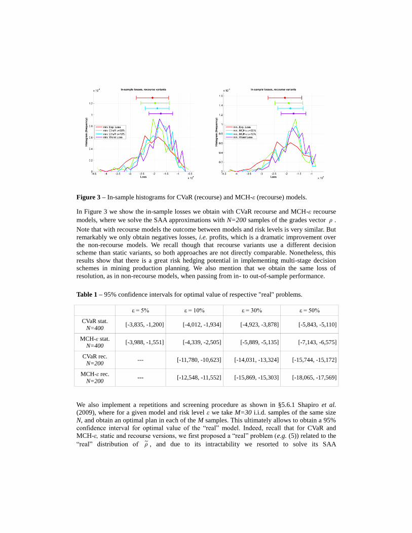
Figure 3 – In-sample histograms for CVaR (recourse) and MCH-ε (recourse) models.

In Figure 3 we show the in-sample losses we obtain with CVaR recourse and MCH-ε recourse

models, where we solve the SAA approximations with N=200 samples of the grades vector ρ .

Note that with recourse models the outcome between models and risk levels is very similar. But

remarkably we only obtain negatives losses, i.e. profits, which is a dramatic improvement over

the non-recourse models. We recall though that recourse variants use a different decision

scheme than static variants, so both approaches are not directly comparable. Nonetheless, this

results show that there is a great risk hedging potential in implementing multi-stage decision

schemes in mining production planning. We also mention that we obtain the same loss of

resolution, as in non-recourse models, when passing from in- to out-of-sample performance.

Table 1 – 95% confidence intervals for optimal value of respective "real" problems.

ε = 5% ε = 10% ε = 30% ε = 50%

CVaR stat.

N=400 [-3,835, -1,200] [-4,012, -1,934] [-4,923, -3,878] [-5,843, -5,110]

MCH-ε stat.

N=400 [-3,988, -1,551] [-4,339, -2,505] [-5,889, -5,135] [-7,143, -6,575]

CVaR rec.

N=200 --- [-11,780, -10,623] [-14,031, -13,324] [-15,744, -15,172]

MCH-ε rec.

N=200 --- [-12,548, -11,552] [-15,869, -15,303] [-18,065, -17,569]

We also implement a repetitions and screening procedure as shown in §5.6.1 Shapiro et al.

(2009), where for a given model and risk level ε we take M=30 i.i.d. samples of the same size

N, and obtain an optimal plan in each of the M samples. This ultimately allows to obtain a 95%

confidence interval for optimal value of the ―real‖ model. Indeed, recall that for CVaR and

MCH-ε, static and recourse versions, we first proposed a ―real‖ problem (e.g. (5)) related to the

―real‖ distribution of ρ~ , and due to its intractability we resorted to solve its SAA

approximation by taking i.i.d. samples (e.g. (6)). This confidence interval then provides an

estimation of the optimal value for the ―true‖ problem, and note that in particular for CVaR

models it provides an estimation of the ―true‖ minimal CVaR possible by a feasible plan. We

refer the reader to §3.3 Lagos (2011) for further details on this procedure. In Table 1 we show

the aforementioned 95% confidence intervals for CVaR and MCH-ε models, static and recourse

versions, for several risk levels ε. Recourse models with ε=5% could not be solved due to either

shortage of memory or no near-optimal solution was found in less than 24 execution hours, so

those fields in Table 1 are left blank. In this regard, the preprocessing step mentioned in the

second section could have made this problem easily solvable, however in this work we focused

solely in evaluating the risk hedging performances of the proposed models. We note that all

interval widths are considerable and as the risk level ε increases the width of the interval

decreases. A heuristic argument for this phenomenon is that with lower risk levels ε we are

focusing on a smaller fraction of the worst losses, which are the most difficult to observe, so

then we need a larger sample size.

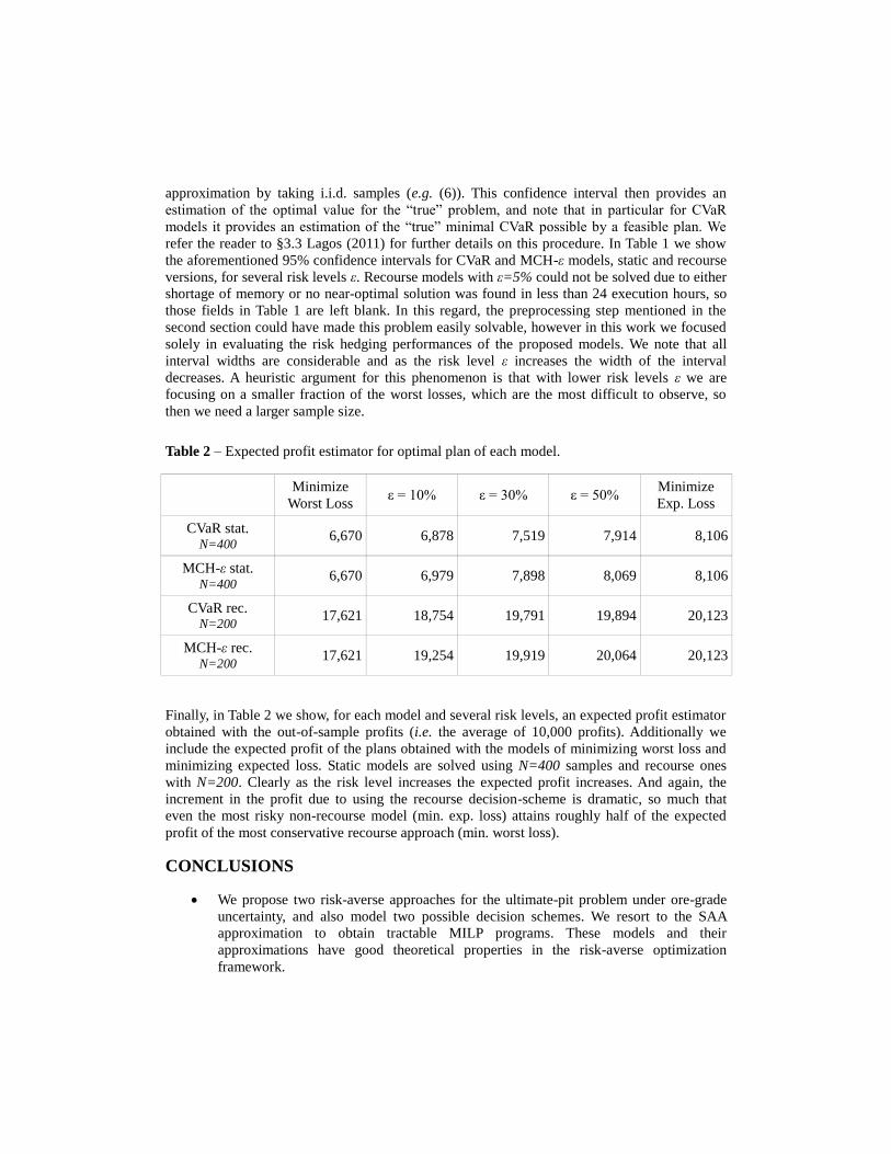
Table 2 – Expected profit estimator for optimal plan of each model.

Minimize

Worst Loss ε = 10% ε = 30% ε = 50%

Minimize

Exp. Loss

CVaR stat. N=400

6,670 6,878 7,519 7,914 8,106

MCH-ε stat. N=400

6,670 6,979 7,898 8,069 8,106

CVaR rec. N=200

17,621 18,754 19,791 19,894 20,123

MCH-ε rec. N=200

17,621 19,254 19,919 20,064 20,123

Finally, in Table 2 we show, for each model and several risk levels, an expected profit estimator

obtained with the out-of-sample profits (i.e. the average of 10,000 profits). Additionally we

include the expected profit of the plans obtained with the models of minimizing worst loss and

minimizing expected loss. Static models are solved using N=400 samples and recourse ones

with N=200. Clearly as the risk level increases the expected profit increases. And again, the

increment in the profit due to using the recourse decision-scheme is dramatic, so much that

even the most risky non-recourse model (min. exp. loss) attains roughly half of the expected

profit of the most conservative recourse approach (min. worst loss).

CONCLUSIONS

We propose two risk-averse approaches for the ultimate-pit problem under ore-grade

uncertainty, and also model two possible decision schemes. We resort to the SAA

approximation to obtain tractable MILP programs. These models and their

approximations have good theoretical properties in the risk-averse optimization

framework.

Computational results show that the classic approach of minimizing expected losses

indeed attain the best on-average results, however such solutions exhibit the highest

probability –between the models compared– of obtaining undesirable outcomes. On

the contrary, the proposed risk-averse models control how much probability the

decision maker is willing to accept of getting undesired losses.

Computational results also indicate that in the proposed models the risk level ε gives a

fine control of the riskiness –or uncertainty of the final outcome– of the obtained plan.

However more certainty is achieved at the expense of obtaining on average higher

losses.

Results also suggest that, even for a small size mine, a very big sample of the ore

grades is needed to capture the distribution of the joint ore grade vector. This is

ultimately a weakness of the chosen modeling, since as the sample size grows the

problems require more computational resources to be solved.

Although the variants with recourse present the same theoretical properties and

practical weaknesses as the static variants –e.g. need for a much bigger sample size to

obtain consistency between in- and out-of-sample performance–, the two-stage

paradigm shows a dramatic improvement over the static one, since it only attains

negative losses. And even though there is not much difference between the

performance of the evaluated recourse variants, even using minimization of expected

loss provides a good protection to uncertainty in the ore-grade. This great potential

suggests exploring the feasibility of implementing in practice sequential decision plans

where relevant decisions are delayed until uncertain parameters are better estimated.

ACKNOWLEDGEMENTS

We gratefully acknowledge the financial support provided by CONICYT with the grant

FONDEF D06-I-1031. We also thank Xavier Emery for providing us with the data used to make

the computational experiments in this work.

REFERENCES

Artzner, P., Delbaen, F., Eber, J. M. and Heath, D. (1999). Coherent measures of risk.

Mathematical finance. v. 9. pp. 203–228.

Benndorf, J. and Dimitrakopoulos, R. (2004). New efficient methods for conditional simulation

of large orebodies. Orebody Modelling and Strategic Mine Planning–Uncertainty and Risk

Management International Symposium 2004. pp. 103–109.

Bertsimas, D. and Brown, D. B. (2009). Constructing uncertainty sets for robust linear

optimization. Operations research. v. 57. pp. 1483–1495.

Caccetta, L. and Hill, S.P. (2003). An application of branch and cut to open pit mine scheduling.

Journal of global optimization. v. 27. pp. 349–365.

Dimitrakopoulos, R. (1998). Conditional simulation algorithms for modelling orebody

uncertainty in open pit optimisation. International Journal of Surface Mining, Reclamation and

Environment. v. 12. pp. 173–179.

Dimitrakopoulos, R., Martinez, L. and Ramazan, S. (2007). A maximum upside/minimum

downside approach to the traditional optimization of open pit mine design. Journal of Mining

Science. v. 43. pp. 73–82.

Dimitrakopoulos, R. (2011). Stochastic optimization for strategic mine planning: A decade of

developments. Journal of Mining Science. v. 47(2). pp. 138–150.

Emery, X. and Lantuéjoul, C. (2006). Tbsim: A computer program for conditional simulation of

three-dimensional gaussian random fields via the turning bands method. Computers &

Geosciences. v. 32. pp. 1615–1628.

Lagos, G. (2011). Estudio de métodos de optimización robusta para el problema de

planificación de producción en minería a cielo abierto. Thesis. Santiago. Universidad de Chile.

Lagos, G., Espinoza, D., Moreno, E. and Amaya, J. (2011). Robust planning for an open-pit

mining problem under ore-grade uncertainty. Electronic Notes in Discrete Mathematics. v. 37.

pp. 15–20.

Linderoth, J., Shapiro, A. and Wright, S. (2006). The empirical behavior of sampling methods

for stochastic programming. Annals of Operations Research. v. 142. pp. 215–241.

Marcotte, D. and Caron, J. (2012). Ultimate open pit stochastic optimization. Computers &

Geosciences. v. 51. pp. 238–246.

Rockafellar, R. T. and Uryasev, S. (2000). Optimization of conditional value-at-risk. Journal of

risk. v. 2. pp. 21–42.

Shapiro, A., Dentcheva, D. and Ruszczynski, A. (2009). Lectures on stochastic programming:

modeling and theory. Philadelphia. SIAM-Society for Industrial and Applied Mathematics.

Vielma, J.P., Espinoza, D. and Moreno, E. (2009). Risk control in ultimate pits using

conditional simulations. Proceedings of APCOM 2009. pp. 107–114.

Lagos, G., Espinoza, D., Moreno, E. and Vielma, J.P. (2012). Restricted risk measures and

robust optimization. Technical report. Atlanta. Georgia Institute of Technology.

Whittle, J. (1988). Beyond optimization in open pit design. Proceedings of the Canadian

Conference on Computer Applications in the Mineral Industries. pp. 331–337.

Whittle, D. and Bozorgebrahimi, A. (2004). Hybrid Pits—Linking conditional simulation and

Lerchs-Grossmann through set theory. Orebody Modelling and Strategic Mine Planning. Perth.

AusIMM (Ed.). pp. 399–404.