Risk and Return - libvolume5.xyzlibvolume5.xyz/.../riskandrequiredreturnpresentation2.pdfDefine risk and return and show how to measure them by calculating expected return, standard

5-1

Chapter 5

Risk and Return

Risk and Return

© Pearson Education Limited 2004Fundamentals of Financial Management, 12/e

Created by: Gregory A. Kuhlemeyer, Ph.D.Carroll College, Waukesha, WI

5-2

After studying Chapter 5,

you should be able to:1. Understand the relationship (or “trade-off”) between risk and return.

2. Define risk and return and show how to measure them by calculating expected return, standard deviation, and coefficient of variation.

3. Discuss the different types of investor attitudes toward risk.

4. Explain risk and return in a portfolio context, and distinguish between individual security and portfolio risk.

5. Distinguish between avoidable (unsystematic) risk and unavoidable (systematic) risk and explain how proper diversification can eliminate one of these risks.

6. Define and explain the capital-asset pricing model (CAPM), beta, and the characteristic line.

7. Calculate a required rate of return using the capital-asset pricing model (CAPM).

8. Demonstrate how the Security Market Line (SML) can be used to describe this relationship between expected rate of return and systematic risk.

9. Explain what is meant by an “efficient financial market” and describe the three levels (or forms) to market efficiency.

5-3

Risk and ReturnRisk and Return

�Defining Risk and Return

�Using Probability Distributions to Measure Risk

�Attitudes Toward Risk

�Risk and Return in a Portfolio Context

�Diversification

�The Capital Asset Pricing Model (CAPM)

�Efficient Financial Markets

�Defining Risk and Return

�Using Probability Distributions to Measure Risk

�Attitudes Toward Risk

�Risk and Return in a Portfolio Context

�Diversification

�The Capital Asset Pricing Model (CAPM)

�Efficient Financial Markets

5-4

Defining ReturnDefining Return

Income received on an investment plus any change in market price, usually expressed as a percent of the beginning market price of the

investment.

Income received on an investment plus any change in market price, usually expressed as a percent of the beginning market price of the

investment.

Dt + (Pt - Pt-1 )

Pt-1

R =

5-5

Return ExampleReturn Example

The stock price for Stock A was $10 per share 1 year ago. The stock is currently

trading at $9.50 per share and shareholders just received a $1 dividend. What return

was earned over the past year?




5-6

Return ExampleReturn Example







$1.00 + ($9.50 - $10.00 )

$10.00R = = 5%

5-7

Defining RiskDefining Risk

What rate of return do you expect on your investment (savings) this year?

What rate will you actually earn?

Does it matter if it is a bank CD or a share of stock?

What rate of return do you expect on your investment (savings) this year?

What rate will you actually earn?

Does it matter if it is a bank CD or a share of stock?

The variability of returns from

those that are expected.

The variability of returns from

those that are expected.

5-8

Determining Expected

Return (Discrete Dist.)


Return (Discrete Dist.)

R = ΣΣΣΣ ( Ri )( Pi )

R is the expected return for the asset,

Ri is the return for the ith possibility,

Pi is the probability of that return occurring,

n is the total number of possibilities.

R = ΣΣΣΣ ( Ri )( Pi )


Ri is the return for the ith possibility,

Pi is the probability of that return occurring,

n is the total number of possibilities.

n

i=1

5-9

How to Determine the Expected

Return and Standard Deviation



Stock BW

Ri Pi (Ri)(Pi)

-.15 .10 -.015

-.03 .20 -.006

.09 .40 .036

.21 .20 .042

.33 .10 .033

Sum 1.00 .090

Stock BW

Ri Pi (Ri)(Pi)

-.15 .10 -.015

-.03 .20 -.006

.09 .40 .036

.21 .20 .042

.33 .10 .033

Sum 1.00 .090

The expected return, R, for Stock BW is .09

or 9%

5-10

Determining Standard

Deviation (Risk Measure)



σσσσ = ΣΣΣΣ ( Ri - R )2( Pi )

Standard Deviation, σσσσ, is a statistical measure of the variability of a distribution

around its mean.

It is the square root of variance.

Note, this is for a discrete distribution.


Standard Deviation, σσσσ, is a statistical measure of the variability of a distribution

around its mean.

It is the square root of variance.

Note, this is for a discrete distribution.

n

i=1

5-11





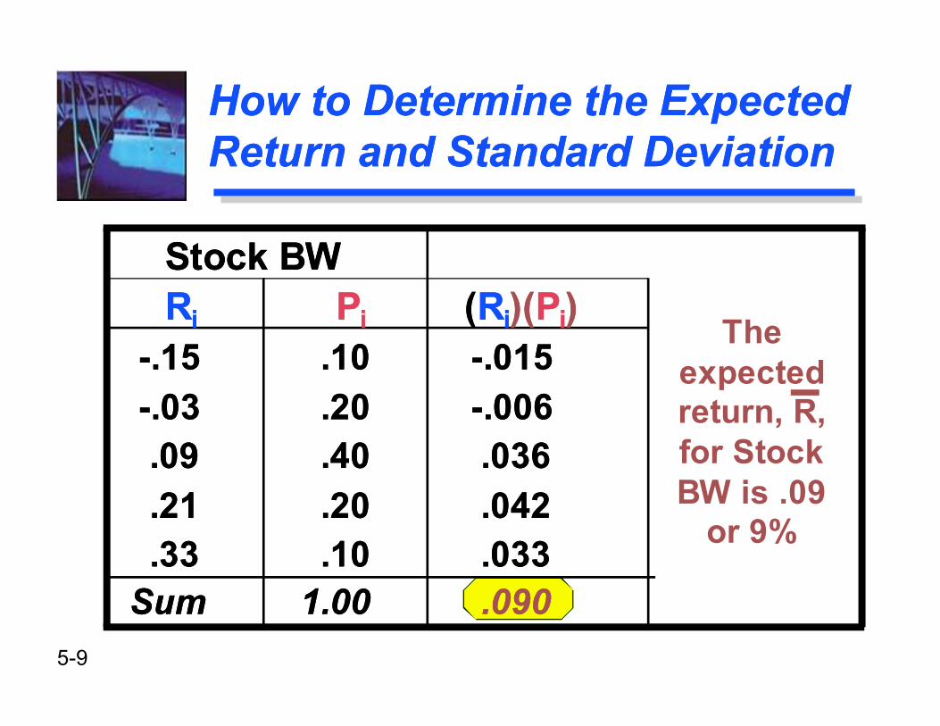
Stock BW

Ri Pi (Ri)(Pi) (Ri - R )2(Pi)

-.15 .10 -.015 .00576

-.03 .20 -.006 .00288

.09 .40 .036 .00000

.21 .20 .042 .00288

.33 .10 .033 .00576

Sum 1.00 .090 .01728

Stock BW

Ri Pi (Ri)(Pi) (Ri - R )2(Pi)

-.15 .10 -.015 .00576

-.03 .20 -.006 .00288

.09 .40 .036 .00000

.21 .20 .042 .00288

.33 .10 .033 .00576

Sum 1.00 .090 .01728

5-12






σσσσ = .01728

σσσσ = .1315 or 13.15%


σσσσ = .01728

σσσσ = .1315 or 13.15%

n

i=1

5-13

Coefficient of VariationCoefficient of Variation

The ratio of the standard deviation of a distribution to the mean of that

distribution.

It is a measure of RELATIVE risk.

CV = σσσσ / R

CV of BW = .1315 / .09 = 1.46

The ratio of the standard deviation of a distribution to the mean of that

distribution.

It is a measure of RELATIVE risk.

CV = σσσσ / R

CV of BW = .1315 / .09 = 1.46

5-14

Discrete vs. Continuous

Distributions

0

0.05

0.1

0.15

0.2

0.25

0.3

0.35

0.4

-15% -3% 9% 21% 33%

Discrete Continuous

0

0.005

0.01

0.015

0.02

0.025

0.03

0.035

-50%

-41%

-32%

-23%

-14%

-5%

4%

13%

22%

31%

40%

49%

58%

67%

5-15


Return (Continuous Dist.)


Return (Continuous Dist.)

R = ΣΣΣΣ ( Ri ) / ( n )


Ri is the return for the ith observation,

n is the total number of observations.

R = ΣΣΣΣ ( Ri ) / ( n )


Ri is the return for the ith observation,

n is the total number of observations.

n

i=1

5-16





n

i=1σσσσ = ΣΣΣΣ ( Ri - R )2

( n )

Note, this is for a continuous distribution where the distribution is for a population. R represents the population mean in this example.

σσσσ = ΣΣΣΣ ( Ri - R )2

( n )

Note, this is for a continuous distribution where the distribution is for a population. R represents the population mean in this example.

5-17

Continuous

Distribution Problem

� Assume that the following list represents the continuous distribution of population returns for a particular investment (even though there are only 10 returns).

�9.6%, -15.4%, 26.7%, -0.2%, 20.9%,

28.3%, -5.9%, 3.3%, 12.2%, 10.5%

�Calculate the Expected Return and Standard Deviation for the populationassuming a continuous distribution.

5-18

Let’s Use the Calculator!Let’s Use the Calculator!

Enter “Data” first. Press:

2nd Data

2nd CLR Work

9.6 ENTER ↓ ↓

-15.4 ENTER ↓ ↓

26.7 ENTER ↓ ↓

� Note, we are inputting data only for the “X” variable and ignoring entries for the “Y” variable in this case.

5-19


Enter “Data” first. Press:

-0.2 ENTER ↓ ↓

20.9 ENTER ↓ ↓

28.3 ENTER ↓ ↓

-5.9 ENTER ↓ ↓

3.3 ENTER ↓ ↓

12.2 ENTER ↓ ↓

10.5 ENTER ↓ ↓

5-20


Examine Results! Press:

2nd Stat

� ↓ through the results.

� Expected return is 9% for the 10 observations. Population standard deviation is 13.32%.

� This can be much quicker than calculating by hand, but slower than using a spreadsheet.

5-21

Certainty Equivalent (CE) is the amount of cash someone would

require with certainty at a point in time to make the individual

indifferent between that certain amount and an amount expected to

be received with risk at the same point in time.

Certainty Equivalent (CE) is the amount of cash someone would

require with certainty at a point in time to make the individual

indifferent between that certain amount and an amount expected to

be received with risk at the same point in time.

Risk AttitudesRisk Attitudes

5-22

Certainty equivalent > Expected value

Risk Preference

Certainty equivalent = Expected value

Risk Indifference

Certainty equivalent < Expected value

Risk Aversion

Most individuals are Risk Averse.

Certainty equivalent > Expected value

Risk Preference

Certainty equivalent = Expected value

Risk Indifference

Certainty equivalent < Expected value

Risk Aversion

Most individuals are Risk Averse.

Risk AttitudesRisk Attitudes

5-23

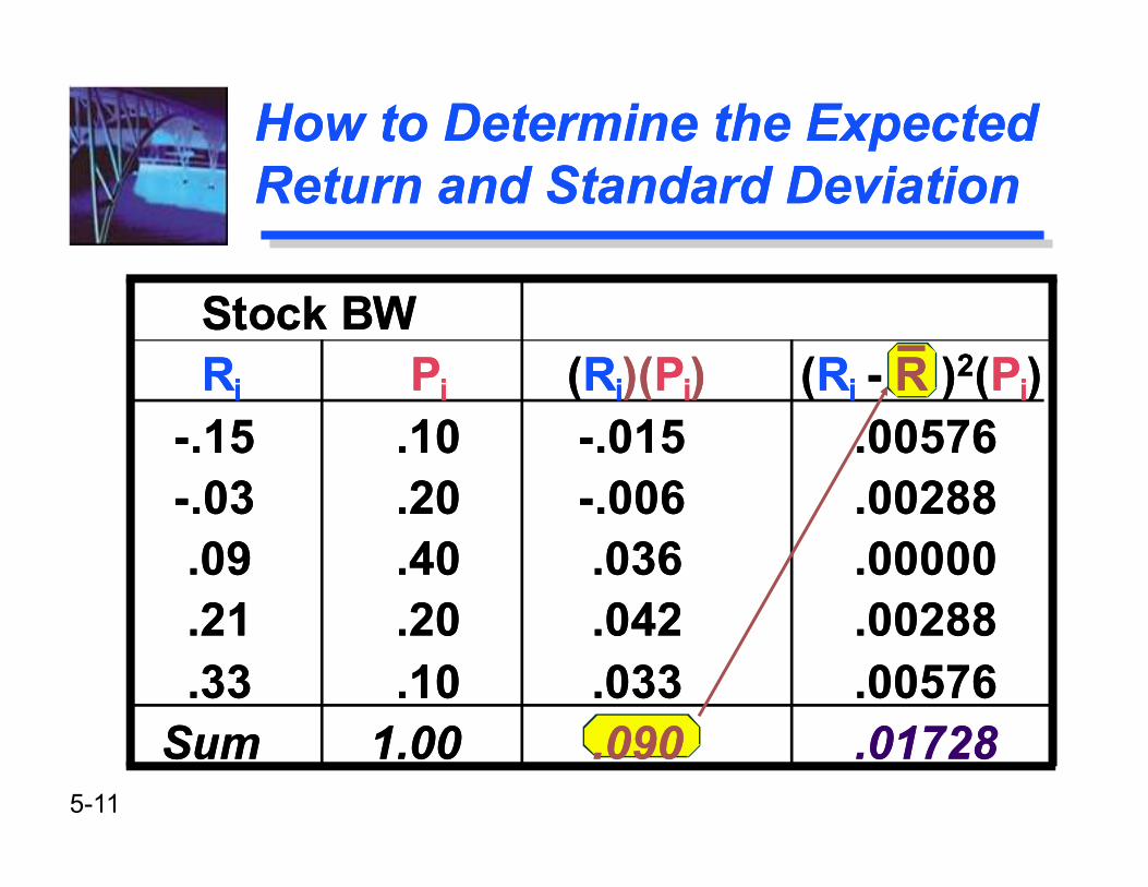
Risk Attitude Example

You have the choice between (1) a guaranteed dollar reward or (2) a coin-flip gamble of

$100,000 (50% chance) or $0 (50% chance). The expected value of the gamble is $50,000.

� Mary requires a guaranteed $25,000, or more, to call off the gamble.

� Raleigh is just as happy to take $50,000 or take the risky gamble.

� Shannon requires at least $52,000 to call off the gamble.

5-24

What are the Risk Attitude tendencies of each?

Risk Attitude ExampleRisk Attitude Example

Mary shows “risk aversion” because her “certainty equivalent” < the expected value of the gamble.

Raleigh exhibits “risk indifference” because her “certainty equivalent” equals the expected value of the gamble.

Shannon reveals a “risk preference” because her “certainty equivalent” > the expected value of the gamble.

Mary shows “risk aversion” because her “certainty equivalent” < the expected value of the gamble.

Raleigh exhibits “risk indifference” because her “certainty equivalent” equals the expected value of the gamble.

Shannon reveals a “risk preference” because her “certainty equivalent” > the expected value of the gamble.

5-25

RP = ΣΣΣΣ ( Wj )( Rj )

RP is the expected return for the portfolio,

Wj is the weight (investment proportion) for the jth asset in the portfolio,

Rj is the expected return of the jth asset,

m is the total number of assets in the portfolio.

RP = ΣΣΣΣ ( Wj )( Rj )

RP is the expected return for the portfolio,


Rj is the expected return of the jth asset,

m is the total number of assets in the portfolio.

Determining Portfolio

Expected Return


Expected Return

m

j=1

5-26


Standard Deviation


Standard Deviation

m

j=1

m

k=1σσσσP = Σ ΣΣ ΣΣ ΣΣ Σ Wj Wk σσσσjk


Wk is the weight (investment proportion) for the kth asset in the portfolio,

σσσσjk is the covariance between returns for the jth and kth assets in the portfolio.

σσσσP = Σ ΣΣ ΣΣ ΣΣ Σ Wj Wk σσσσjk


Wk is the weight (investment proportion) for the kth asset in the portfolio,

σσσσjk is the covariance between returns for the jth and kth assets in the portfolio.

5-27

Tip Slide: Appendix A

Slides 5-28 through 5-30 and 5-33 through 5-36

assume that the student has read Appendix A in

Chapter 5

5-28

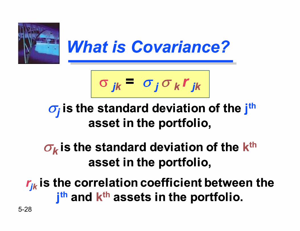
What is Covariance?What is Covariance?

σσσσ jk = σ σ σ σ j σ σ σ σ k r jk

σσσσj is the standard deviation of the jth

asset in the portfolio,

σσσσk is the standard deviation of the kth


rjk is the correlation coefficient between the jth and kth assets in the portfolio.

σσσσ jk = σ σ σ σ j σ σ σ σ k r jk

σσσσj is the standard deviation of the jth


σσσσk is the standard deviation of the kth


rjk is the correlation coefficient between the jth and kth assets in the portfolio.

5-29

Correlation CoefficientCorrelation Coefficient

A standardized statistical measure

of the linear relationship between

two variables.

Its range is from -1.0 (perfect negative correlation), through 0(no correlation), to +1.0 (perfect

positive correlation).

A standardized statistical measure

of the linear relationship between

two variables.

Its range is from -1.0 (perfect negative correlation), through 0(no correlation), to +1.0 (perfect

positive correlation).

5-30

Variance - Covariance MatrixVariance - Covariance Matrix

A three asset portfolio:

Col 1 Col 2 Col 3

Row 1 W1W1σσσσ1,1 W1W2σσσσ1,2 W1W3σσσσ1,3



σσσσj,k = is the covariance between returns for the jth and kth assets in the portfolio.

A three asset portfolio:

Col 1 Col 2 Col 3




σσσσj,k = is the covariance between returns for the jth and kth assets in the portfolio.

5-31

You are creating a portfolio of Stock D and Stock BW (from earlier). You are investing $2,000 in

Stock BW and $3,000 in Stock D. Remember that the expected return and standard deviation ofStock BW is 9% and 13.15% respectively. The

expected return and standard deviation of Stock D is 8% and 10.65% respectively. The correlation

coefficient between BW and D is 0.75.

What is the expected return and standard deviation of the portfolio?

You are creating a portfolio of Stock D and Stock BW (from earlier). You are investing $2,000 in

Stock BW and $3,000 in Stock D. Remember that the expected return and standard deviation ofStock BW is 9% and 13.15% respectively. The

expected return and standard deviation of Stock D is 8% and 10.65% respectively. The correlation

coefficient between BW and D is 0.75.

What is the expected return and standard deviation of the portfolio?

Portfolio Risk and

Expected Return Example

Portfolio Risk and

Expected Return Example

5-32


Expected Return


Expected Return

WBW = $2,000 / $5,000 = .4

WD = $3,000 / $5,000 = .6

RP = (WBW)(RBW) + (WD)(RD)

RP = (.4)(9%) + (.6)(8%)

RP = (3.6%) + (4.8%) = 8.4%

WBW = $2,000 / $5,000 = .4

WD = $3,000 / $5,000 = .6

RP = (WBW)(RBW) + (WD)(RD)

RP = (.4)(9%) + (.6)(8%)

RP = (3.6%) + (4.8%) = 8.4%

5-33

Two-asset portfolio:

Col 1 Col 2

Row 1 WBW WBW σσσσBW,BW WBW WD σσσσBW,D

Row 2 WD WBW σσσσD,BW WD WD σσσσD,D

This represents the variance - covariance matrix for the two-asset portfolio.


Col 1 Col 2

Row 1 WBW WBW σσσσBW,BW WBW WD σσσσBW,D

Row 2 WD WBW σσσσD,BW WD WD σσσσD,D

This represents the variance - covariance matrix for the two-asset portfolio.


Standard Deviation


Standard Deviation

5-34


Col 1 Col 2

Row 1 (.4)(.4)(.0173) (.4)(.6)(.0105)

Row 2 (.6)(.4)(.0105) (.6)(.6)(.0113)

This represents substitution into the variance - covariance matrix.


Col 1 Col 2

Row 1 (.4)(.4)(.0173) (.4)(.6)(.0105)

Row 2 (.6)(.4)(.0105) (.6)(.6)(.0113)

This represents substitution into the variance - covariance matrix.


Standard Deviation


Standard Deviation

5-35


Col 1 Col 2

Row 1 (.0028) (.0025)

Row 2 (.0025) (.0041)

This represents the actual element values in the variance - covariance matrix.


Col 1 Col 2

Row 1 (.0028) (.0025)

Row 2 (.0025) (.0041)

This represents the actual element values in the variance - covariance matrix.


Standard Deviation


Standard Deviation

5-36


Standard Deviation


Standard Deviation

σσσσP = .0028 + (2)(.0025) + .0041

σσσσP = SQRT(.0119)

σσσσP = .1091 or 10.91%

A weighted average of the individual standard deviations is INCORRECT.

σσσσP = .0028 + (2)(.0025) + .0041

σσσσP = SQRT(.0119)

σσσσP = .1091 or 10.91%

A weighted average of the individual standard deviations is INCORRECT.

5-37


Standard Deviation


Standard Deviation

The WRONG way to calculate is a weighted average like:

σσσσP = .4 (13.15%) + .6(10.65%)

σσσσP = 5.26 + 6.39 = 11.65%

10.91% = 11.65%

This is INCORRECT.

The WRONG way to calculate is a weighted average like:

σσσσP = .4 (13.15%) + .6(10.65%)

σσσσP = 5.26 + 6.39 = 11.65%

10.91% = 11.65%

This is INCORRECT.

5-38

Stock C Stock D Portfolio

Return 9.00% 8.00% 8.64%

Stand.

Dev. 13.15% 10.65% 10.91%

CV 1.46 1.33 1.26

The portfolio has the LOWEST coefficient of variation due to diversification.

Stock C Stock D Portfolio

Return 9.00% 8.00% 8.64%

Stand.

Dev. 13.15% 10.65% 10.91%

CV 1.46 1.33 1.26

The portfolio has the LOWEST coefficient of variation due to diversification.

Summary of the Portfolio

Return and Risk Calculation

Summary of the Portfolio

Return and Risk Calculation

5-39

Combining securities that are not perfectly, positively correlated reduces risk.

Combining securities that are not perfectly, positively correlated reduces risk.

Diversification and the

Correlation Coefficient

Diversification and the

Correlation CoefficientIN

VE

ST

ME

NT

RE

TU

RN

TIME TIMETIME

SECURITY E SECURITY FCombination

E and F

5-40

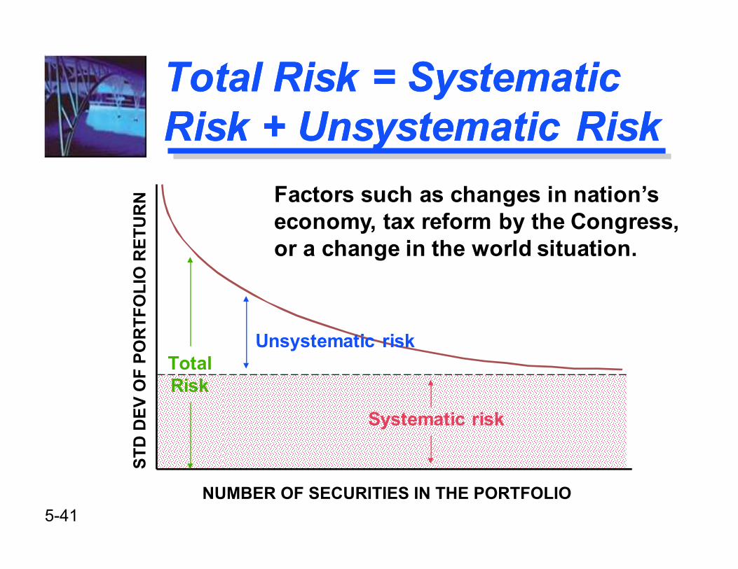
Systematic Risk is the variability of return on stocks or portfolios associated with

changes in return on the market as a whole.

Unsystematic Risk is the variability of return on stocks or portfolios not explained by

general market movements. It is avoidable through diversification.

Systematic Risk is the variability of return on stocks or portfolios associated with

changes in return on the market as a whole.

Unsystematic Risk is the variability of return on stocks or portfolios not explained by

general market movements. It is avoidable through diversification.

Total Risk = Systematic

Risk + Unsystematic Risk



Total Risk = Systematic Risk +Unsystematic Risk

5-41





TotalRisk

Unsystematic risk

Systematic risk

ST

D D

EV

OF

PO

RT

FO

LIO

RE

TU

RN

NUMBER OF SECURITIES IN THE PORTFOLIO

Factors such as changes in nation’s economy, tax reform by the Congress,or a change in the world situation.

5-42





TotalRisk

Unsystematic risk

Systematic risk

ST

D D

EV

OF

PO

RT

FO

LIO

RE

TU

RN

NUMBER OF SECURITIES IN THE PORTFOLIO

Factors unique to a particular companyor industry. For example, the death of akey executive or loss of a governmentaldefense contract.

5-43

CAPM is a model that describes the relationship between risk and

expected (required) return; in this model, a security’s expected

(required) return is the risk-free rate plus a premium based on the systematic risk of the security.

CAPM is a model that describes the relationship between risk and

expected (required) return; in this model, a security’s expected

(required) return is the risk-free rate plus a premium based on the systematic risk of the security.

Capital Asset

Pricing Model (CAPM)

Capital Asset

Pricing Model (CAPM)

5-44

1. Capital markets are efficient.

2. Homogeneous investor expectations over a given period.

3. Risk-free asset return is certain (use short- to intermediate-term Treasuries as a proxy).

4. Market portfolio contains onlysystematic risk (use S&P 500 Indexor similar as a proxy).

1. Capital markets are efficient.

2. Homogeneous investor expectations over a given period.

3. Risk-free asset return is certain (use short- to intermediate-term Treasuries as a proxy).

4. Market portfolio contains onlysystematic risk (use S&P 500 Indexor similar as a proxy).

CAPM AssumptionsCAPM Assumptions

5-45

Characteristic LineCharacteristic Line

EXCESS RETURNON STOCK

EXCESS RETURNON MARKET PORTFOLIO

Beta =RiseRun

Narrower spreadis higher correlation

Characteristic Line

5-46

Calculating “Beta”

on Your Calculator

Time Pd. Market My Stock

1 9.6% 12%

2 -15.4% -5%

3 26.7% 19%

4 -.2% 3%

5 20.9% 13%

6 28.3% 14%

7 -5.9% -9%

8 3.3% -1%

9 12.2% 12%

10 10.5% 10%

The Marketand My Stock

returns are “excess

returns” and have the

riskless rate already

subtracted.

5-47


on Your Calculator

� Assume that the previous continuous distribution problem represents the “excess returns” of the market portfolio (it may still be in your calculator data worksheet -- 2nd Data ).

� Enter the excess market returns as “X”

observations of: 9.6%, -15.4%, 26.7%, -0.2%, 20.9%, 28.3%, -5.9%, 3.3%, 12.2%, and 10.5%.

� Enter the excess stock returns as “Y” observations of: 12%, -5%, 19%, 3%, 13%, 14%, -9%, -1%, 12%, and 10%.

5-48


on Your Calculator

�Let us examine again the statistical results (Press 2nd and then Stat )

� The market expected return and standard deviation is 9% and 13.32%. Your stock expected return and standard deviation is

6.8% and 8.76%.

� The regression equation is Y=a+bX. Thus, our characteristic line is Y = 1.4448 + 0.595 X and

indicates that our stock has a beta of 0.595.

5-49

An index of systematic risk.

It measures the sensitivity of a stock’s returns to changes in

returns on the market portfolio.

The beta for a portfolio is simply a weighted average of the individual

stock betas in the portfolio.

An index of systematic risk.

It measures the sensitivity of a stock’s returns to changes in

returns on the market portfolio.

The beta for a portfolio is simply a weighted average of the individual

stock betas in the portfolio.

What is Beta?What is Beta?

5-50

Characteristic Lines

and Different Betas

Characteristic Lines

and Different Betas

EXCESS RETURNON STOCK

EXCESS RETURNON MARKET PORTFOLIO

Beta < 1(defensive)

Beta = 1

Beta > 1(aggressive)

Each characteristic line has a

different slope.

5-51

Rj is the required rate of return for stock j,

Rf is the risk-free rate of return,

ββββ j is the beta of stock j (measures systematic risk of stock j),

RM is the expected return for the market portfolio.

Rj is the required rate of return for stock j,

Rf is the risk-free rate of return,

ββββ j is the beta of stock j (measures systematic risk of stock j),

RM is the expected return for the market portfolio.

Security Market LineSecurity Market Line

Rj = Rf + ββββj(RM - Rf)

5-52


Rj = Rf + ββββj(RM - Rf)

ββββM = 1.0

Systematic Risk (Beta)

Rf

RM

Req

uir

ed

Retu

rn

RiskPremium

Risk-freeReturn

5-53


� Obtaining Betas

� Can use historical data if past best represents the expectations of the future

� Can also utilize services like Value Line, Ibbotson Associates, etc.

� Adjusted Beta

� Betas have a tendency to revert to the mean of 1.0

� Can utilize combination of recent beta and mean

� 2.22 (.7) + 1.00 (.3) = 1.554 + 0.300 = 1.854 estimate

� Obtaining Betas

� Can use historical data if past best represents the expectations of the future

� Can also utilize services like Value Line, Ibbotson Associates, etc.

� Adjusted Beta

� Betas have a tendency to revert to the mean of 1.0

� Can utilize combination of recent beta and mean

� 2.22 (.7) + 1.00 (.3) = 1.554 + 0.300 = 1.854 estimate

5-54

Lisa Miller at Basket Wonders is attempting to determine the rate of return required by their stock investors. Lisa is

using a 6% Rf and a long-term market expected rate of return of 10%. A stock analyst following the firm has calculated

that the firm beta is 1.2. What is the required rate of return on the stock of

Basket Wonders?

Lisa Miller at Basket Wonders is attempting to determine the rate of return required by their stock investors. Lisa is

using a 6% Rf and a long-term market expected rate of return of 10%. A stock analyst following the firm has calculated

that the firm beta is 1.2. What is the required rate of return on the stock of

Basket Wonders?

Determination of the

Required Rate of Return



5-55

RBW = Rf + ββββj(RM - Rf)

RBW = 6% + 1.2(10% - 6%)

RBW = 10.8%

The required rate of return exceeds the market rate of return as BW’s

beta exceeds the market beta (1.0).

RBW = Rf + ββββj(RM - Rf)

RBW = 6% + 1.2(10% - 6%)

RBW = 10.8%

The required rate of return exceeds the market rate of return as BW’s

beta exceeds the market beta (1.0).

BWs Required

Rate of Return

BWs Required

Rate of Return

5-56

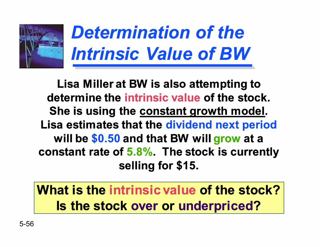
Lisa Miller at BW is also attempting to determine the intrinsic value of the stock. She is using the constant growth model.

Lisa estimates that the dividend next period will be $0.50 and that BW will grow at a

constant rate of 5.8%. The stock is currently selling for $15.

What is the intrinsic value of the stock? Is the stock over or underpriced?

Lisa Miller at BW is also attempting to determine the intrinsic value of the stock. She is using the constant growth model.

Lisa estimates that the dividend next period will be $0.50 and that BW will grow at a

constant rate of 5.8%. The stock is currently selling for $15.

What is the intrinsic value of the stock? Is the stock over or underpriced?


Intrinsic Value of BW



5-57

The stock is OVERVALUED as the market price ($15) exceeds

the intrinsic value ($10).

The stock is OVERVALUED as the market price ($15) exceeds

the intrinsic value ($10).





$0.5010.8% - 5.8%

IntrinsicValue

=

= $10

5-58


Systematic Risk (Beta)

Rf

Req

uir

ed

Retu

rn

Direction ofMovement

Direction ofMovement

Stock Y (Overpriced)

Stock X (Underpriced)

5-59

Small-firm Effect

Price / Earnings Effect

January Effect

These anomalies have presented serious challenges to the CAPM

theory.

Small-firm Effect

Price / Earnings Effect

January Effect

These anomalies have presented serious challenges to the CAPM

theory.





Documents

Risk and Return - libvolume5.xyzlibvolume5.xyz/.../riskandrequiredreturnpresentation2.pdfDefine risk and return and show how to measure them by calculating expected return, standard