Risk and Economic Under-Specialization:Why the Pin-Maker Grows Cassava on the

Side

Ajay Shenoy∗

University of Michigan, Ann Arbor

September 13, 2013First Version: October 08, 2012

Abstract

Why do the poor have so many economic activities? According to onetheory the poor do not specialize because relying on one income sourceis risky. I test the theory by measuring the response of Thai rice farmersto conditional volatility in the international rice price. Uninsured house-holds expecting a harvest reduce specialization by .18 percent when volatil-ity rises by 1 percent. I confirm the decrease in specialization costs house-holds foregone revenue. I find no evidence for the alternate explanationthat households under-specialize because they cannot afford lumpy busi-ness investments. (JEL Codes: D13, O12, D81)

∗Email at shenoy@umich.edu. File formatting based on a stylesheet by Charles Jones. Spe-cial thanks to Raj Arunachalam, David Lam, Jeff Smith, David Weil, Anja Sautmann, Chris Udry,Silvia Prina, Stefanie Stantcheva, seminar participants at Michigan and Brown, and conferenceattendees at PacDev and MWIEDC in 2013 for helpful comments and advice. I am also gratefulto Robert Townsend and the Townsend Thai Project for collecting and distributing the data Iuse for this project.

2 AJAY SHENOY

1 Introduction

To take...the trade of the pin-maker...in the way in which this business

is now carried on...it is divided into a number of branches...One man

draws out the wire, another straights it, a third cuts it...I have seen a

small manufactory of this kind where ten men only were employed...

Those ten persons, therefore, could make among them upwards of

forty-eight thousand pins in a day...But if they had all wrought sepa-

rately and independently...they certainly could not each of them have

made twenty, perhaps not one pin in a day...

-Adam Smith, Wealth of Nations

The secret of the pin-maker is also the secret of any modern society: spe-

cialization is efficient and raises aggregate output. It seems to be no secret at

all. In no modern economy do doctors grow their own wheat or farmers set

their own bones. Yet in developing countries farmers run general stores, tai-

lors labor in their neighbors’ fields, and people of all occupations grow cassava.

Banerjee and Duflo (2007) look across the developing world and find very few

households that specialize in one economic activity. If specialization really does

increase everyone’s income, why would the households with the least income

fail to specialize?

Almost by definition a developing country has weak insurance and credit

markets, so it is no surprise that the two leading explanations blame income

risk and credit constraints for under-specialization. The first compares a poor

household choosing its activities to an investor choosing her stock portfolio. No

investor pours all her savings into one stock because a bad year could leave her

penniless. No household will spend all its time working at a single activity when

a bad harvest or slow sales could leave it in starvation. The other explanation

assumes a household cannot grow its business without making a lumpy invest-

ment. A household can hand-sew and sell a few shirts but must buy a sewing

machine to clothe the entire village. If it cannot afford the machine and cannot

get a loan it might sell bread to supplement its income. The two theories—risky

income and lumpy investments—blame different market failures and prescribe

different solutions for under-specialization. To my knowledge no one has for-

RISK AND ECONOMIC UNDER-SPECIALIZATION 3

malized and tested them with plausibly exogenous variation.

I test both theories using data on Thai rice farmers. I formalize the risky in-

come theory in a simple model where households pay fixed costs to enter eco-

nomic activities. A household enters more activities when its primary activity

becomes riskier, and the resulting under-specialization reduces the household’s

revenue. To test the model I measure how rice farmers respond to changes in

the mean and volatility of the international rice price. I use a time series of the

international rice price to calculate its monthly volatility. I then identify in a

monthly survey the households who expect a rice harvest soon. Higher volatil-

ity in the price of rice raises the riskiness of their income. By comparing their

response to the responses of households who do not farm rice and those that

farm but expect no harvest, I identify the causal effect of riskier income on spe-

cialization. I confirm the response is strongest among households without the

informal insurance of income transfers. Among the uninsured a 10 percent in-

crease in volatility causes a .18 percent decrease in specialization, as much as a

3 percent increase in the average price.

A household still expecting its harvest sells no rice, so the mean and variance

of the rice price change the number of economic activities without directly af-

fecting current revenue. Using them to instrument for activities I confirm that

a failure to specialize lowers household revenue, exactly the opposite of what a

simple OLS regression shows.

Finally, I test the alternative theory of under-specialization—the theory of

lumpy investments and credit constraints—using a quasi-experimental credit

injection. I exploit the Million Baht Program (Kaboski and Townsend, 2011) to

test whether relaxing credit constraints decreases the number of activities but

find no evidence.

2 Background

Smith gives two parables of under-specialization: the parable of the pin-maker

and the parable of the nail-maker. The pin-maker stops switching between

tasks and uses the time saved to work more at one task. The nail-maker learns

more about nails than generalist blacksmiths and uses the knowledge to pro-

4 AJAY SHENOY

duce more nails. The man who wastes his time juggling ten jobs differs from

the man who wasted his ability learning ten trades. They lose income for differ-

ent reasons, and the difference matters because I say nothing about learning.

Others have worked to isolate the effect of risk on learning, investment, and

occupation. By distinguishing expected from unexpected shocks Jacoby and

Skoufias (1997) find both credit and insurance market failures reduce child-

hood schooling. Rosenzweig and Binswanger (1993) find that greater variability

in the onset of the monsoon predicts a safer but less profitable mix of agricul-

tural investment among poor households. Bandyopadhyay and Skoufias (2012)

find that Bangladeshi spouses who farm land in riskier climates differ more

in occupation unless floods, which make rainfall less important, are common.

Government safety nets reduce the effect and less specialized households have

lower consumption. Menon (2009) finds riskier climate predicts less special-

ization in rural Nepal. These studies do not, however, prove risk causes under-

specialization. Less schooling and less profitable investments need not affect

specialization. Households who live in risky climates may differ from those in

safe climates, and the unobserved difference may bias estimates of risk’s impact

on specialization.

I use exogenous variation in risk—changes in the volatility of the interna-

tional rice price—to test if risk causes under-specialization. To explain the styl-

ized fact Banerjee and Duflo (2007) find I measure specialization with the num-

ber of economic activities . I use the same variation to confirm under-specialization

is costly and to test other predictions of the model of Section 3. The story I

test, however, is the story of the pin-maker: moving between many small tasks

wastes time. I measure short-term responses to short-term rises in price volatil-

ity: a rice farmer expecting a harvest takes on extra activities when prices turn

volatile. Future research must answer whether risk makes learning too many

trades attractive: the story of the nail-maker.

3 A Model of Risk and Specialization

The model I build is by no means the model of risk and under-specialization.

The crucial assumption—that labor yields increasing but uncertain returns that

RISK AND ECONOMIC UNDER-SPECIALIZATION 5

are not perfectly correlated across different economic activities—need not be

made as I make it with linear returns and a fixed cost for each activity. My im-

plementation does, however, make testable predictions without too much alge-

bra.1

3.1 Setup

Each household has one primary economic activity and may enter side activi-

ties if it pays a fixed cost for each. It allocates one unit of labor across the pri-

mary and however many side activities it enters. Labor produces a constant

return in revenue, and the household does not know each activitys return when

it enters activities and allocates labor.2

that net of fixed costs the return to an activity have increasing returns over

some region that includes

The household solves

maxM,Lp,{Lsm}

E[−e−αC ]

subject to

C = Y = wpLp +∑m∈M

wsmLsm −MF

Lp +∑m

Lsm = 1

The household picks the number of side activities M ≥ 0 and the labor allo-

cated to the primary activity Lp and each side activity {Lsm}m∈M . It has constant

absolute risk-aversion preferences with risk-aversion α. It consumes its rev-

enue, which is the sum of revenue from primary (p) and side (s) activities mi-

nus fixed costs. The primary and side activities yield returns wp and {wsm}m∈M ,

which are independent normal random variables withwp ∼ N(wp, σ2p) andwsm ∼

1See Appendix E for an alternate model that makes similar predictions without fixed costs.2Constant returns make the model simpler, but risk will drive households to under-

specialize even without it when fixed-costs are large. What matters is the average return—revenue minus fixed cost, per unit of labor—be increasing at least initially.

6 AJAY SHENOY

N(ws, σ2s) for each m. Assume the secondary activities yield weakly lower ex-

pected returns: wp ≥ ws.

If returns to the primary activity were certain—say from a salaried govern-

ment job—the household would perfectly specialize (M = 0). Specialization

spares the household fixed costs and earns a higher return. Risk is the only rea-

son the household might not specialize.

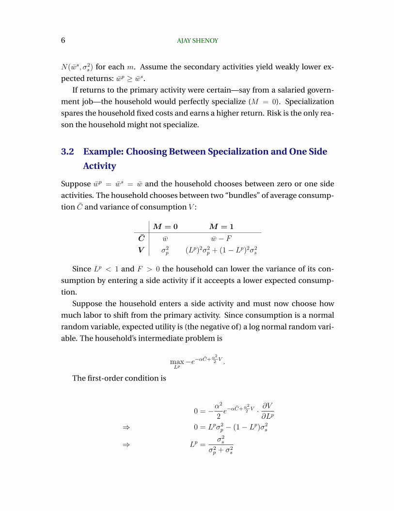
3.2 Example: Choosing Between Specialization and One Side

Activity

Suppose wp = ws = w and the household chooses between zero or one side

activities. The household chooses between two “bundles” of average consump-

tion C and variance of consumption V :

M = 0 M = 1

C w w − FV σ2

p (Lp)2σ2p + (1− Lp)2σ2

s

Since Lp < 1 and F > 0 the household can lower the variance of its con-

sumption by entering a side activity if it acceepts a lower expected consump-

tion.

Suppose the household enters a side activity and must now choose how

much labor to shift from the primary activity. Since consumption is a normal

random variable, expected utility is (the negative of) a log normal random vari-

able. The household’s intermediate problem is

maxLp−e−αC+α2

2V .

The first-order condition is

0 = −α2

2e−αC+α2

2V · ∂V

∂Lp

⇒ 0 = Lpσ2p − (1− Lp)σ2

s

⇒ Lp =σ2s

σ2p + σ2

s

RISK AND ECONOMIC UNDER-SPECIALIZATION 7

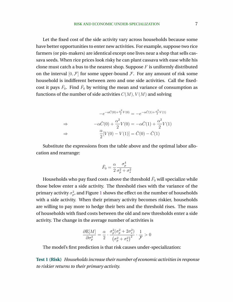
Let the fixed cost of the side activity vary across households because some

have better opportunities to enter new activities. For example, suppose two rice

farmers (or pin-makers) are identical except one lives near a shop that sells cas-

sava seeds. When rice prices look risky he can plant cassava with ease while his

clone must catch a bus to the nearest shop. Suppose F is uniformly distributed

on the interval [0,F ] for some upper-bound F . For any amount of risk some

household is indifferent between zero and one side activities. Call the fixed-

cost it pays F0. Find F0 by writing the mean and variance of consumption as

functions of the number of side activities C(M), V (M) and solving

−e−αC(0)+α2

2V (0) = −e−αC(1)+α2

2V (1)

⇒ −αC(0) +α2

2V (0) = −αC(1) +

α2

2V (1)

⇒ α

2[V (0)− V (1)] = C(0)− C(1)

Substitute the expressions from the table above and the optimal labor allo-

cation and rearrange:

F0 =α

2

σ4p

σ2p + σ2

s

Households who pay fixed costs above the threshold F0 will specialize while

those below enter a side activity. The threshold rises with the variance of the

primary activity σ2p, and Figure 1 shows the effect on the number of households

with a side activity. When their primary activity becomes riskier, households

are willing to pay more to hedge their bets and the threshold rises. The mass

of households with fixed costs between the old and new thresholds enter a side

activity. The change in the average number of activities is

∂E[M ]

∂σ2p

=α

2·σ2p(σ

2p + 2σ2

s)(σ2p + σ2

s

)2 ·1

F> 0

The model’s first prediction is that risk causes under-specialization:

Test 1 (Risk) Households increase their number of economic activities in response

to riskier returns to their primary activity.

8 AJAY SHENOY

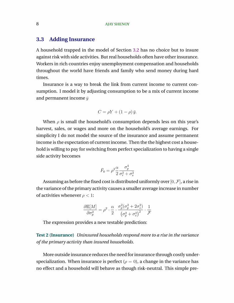
3.3 Adding Insurance

A household trapped in the model of Section 3.2 has no choice but to insure

against risk with side activities. But real households often have other insurance.

Workers in rich countries enjoy unemployment compensation and households

throughout the world have friends and family who send money during hard

times.

Insurance is a way to break the link from current income to current con-

sumption. I model it by adjusting consumption to be a mix of current income

and permanent income y

C = ρY + (1− ρ) y.

When ρ is small the household’s consumption depends less on this year’s

harvest, sales, or wages and more on the household’s average earnings. For

simplicity I do not model the source of the insurance and assume permanent

income is the expectation of current income. Then the the highest cost a house-

hold is willing to pay for switching from perfect specialization to having a single

side activity becomes

F0 = ρ2α

2

σ4p

σ2r + σ2

s

Assuming as before the fixed cost is distributed uniformly over [0,F ], a rise in

the variance of the primary activity causes a smaller average increase in number

of activities whenever ρ < 1:

∂E[M ]

∂σ2p

= ρ2 · α2·σ2p(σ

2p + 2σ2

s)(σ2p + σ2

s

)2 ·1

F

The expression provides a new testable prediction:

Test 2 (Insurance) Uninsured households respond more to a rise in the variance

of the primary activity than insured households.

More outside insurance reduces the need for insurance through costly under-

specialization. When insurance is perfect (ρ = 0), a change in the variance has

no effect and a household will behave as though risk-neutral. This simple pre-

RISK AND ECONOMIC UNDER-SPECIALIZATION 9

diction is also a reality check—it must hold if the effects I find in the empirical

section are actual responses to risk.

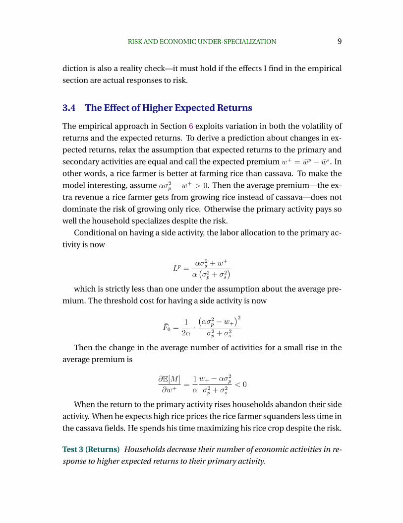
3.4 The Effect of Higher Expected Returns

The empirical approach in Section 6 exploits variation in both the volatility of

returns and the expected returns. To derive a prediction about changes in ex-

pected returns, relax the assumption that expected returns to the primary and

secondary activities are equal and call the expected premium w+ = wp − ws. In

other words, a rice farmer is better at farming rice than cassava. To make the

model interesting, assume ασ2p − w+ > 0. Then the average premium—the ex-

tra revenue a rice farmer gets from growing rice instead of cassava—does not

dominate the risk of growing only rice. Otherwise the primary activity pays so

well the household specializes despite the risk.

Conditional on having a side activity, the labor allocation to the primary ac-

tivity is now

Lp =ασ2

s + w+

α(σ2p + σ2

s

)which is strictly less than one under the assumption about the average pre-

mium. The threshold cost for having a side activity is now

F0 =1

2α·(ασ2

p − w+

)2

σ2p + σ2

s

Then the change in the average number of activities for a small rise in the

average premium is

∂E[M ]

∂w+=

1

α

w+ − ασ2p

σ2p + σ2

s

< 0

When the return to the primary activity rises households abandon their side

activity. When he expects high rice prices the rice farmer squanders less time in

the cassava fields. He spends his time maximizing his rice crop despite the risk.

Test 3 (Returns) Households decrease their number of economic activities in re-

sponse to higher expected returns to their primary activity.

10 AJAY SHENOY

3.5 Linking Economic Activities to Revenue

Taking on additional side activities lowers the household’s expected total rev-

enue. But the empirical strategy of Section 6 examines rice farmers who ex-

pect but have not yet collected a harvest. By construction it cannot test predic-

tions about total revenue. I must derive the model’s predictions about under-

specialization and revenue from side activities: what happens to the rice farmer’s

revenue from cassava when he starts baking and selling bread.

Consider again the simple case where returns are equal but suppose house-

holds can choose any number of activities. The general expression for labor

allocated to each side activity is

Lsm =1

M·

Mσ2p

Mσ2p + σ2

s

Let ys =∑

m∈M wmLsm − MF denote the total revenue from side activities.

For simplicity treat the number of activitiesM as continuous. Holding a house-

hold’s cost of additional activities fixed, a small increase in the number of activ-

ities changes side revenue on average by

EF[∂ys

∂M

]= −E[F ] + E

[wσ2

pσ2s(

Mσ2p + σ2

s

)2

]

where the expectation with respect to F is a population average. The aver-

age change in side revenue, which corresponds to the instrumental variables

coefficient estimated in Section 7.1, has two parts. The first part is the fixed cost

of extra activities, and it lowers side revenue. A rice farmer who starts baking

bread must buy flour. The second part is the labor effect, and it raises side rev-

enue. A rice farmer who switches from just growing cassava on the side to also

baking bread will shift labor away from rice farming towards cassava and bread.

In the language of lotteries, side activities as a whole are a safer bet when they

include both cassava and baking. The farmer bets more on them—he raises∑Lsm—and less on rice farming—he lowers Lp. When he works more at his side

activities they produce more revenue on average.

The total change in side revenue might not be negative: the labor allocation

RISK AND ECONOMIC UNDER-SPECIALIZATION 11

effect might dominate the fixed cost of extra activities. Then a decrease in side

revenue from additional activities implies a cost to specialization, yet the con-

verse need not be true. But for the current endeavor I do not need equivalency.

A decrease in side revenue from more activities, which is exactly what I find, will

validate the theory of costly under-specialization.

Test 4 (Cost) The average effect on revenue of more activities is negative only if

under-specialization is costly.

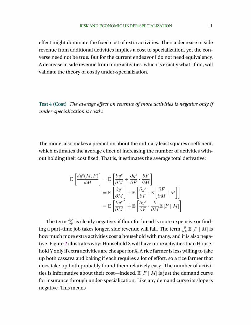
The model also makes a prediction about the ordinary least squares coefficient,

which estimates the average effect of increasing the number of activities with-

out holding their cost fixed. That is, it estimates the average total derivative:

E[dys(M,F )

dM

]= E

[∂ys

∂M+∂ys

∂F· ∂F∂M

]= E

[∂ys

∂M

]+ E

[∂ys

∂F· E[∂F

∂M|M

]]= E

[∂ys

∂M

]+ E

[∂ys

∂F· ∂

∂ME [F |M ]

]The term ∂ys

∂Fis clearly negative: if flour for bread is more expensive or find-

ing a part-time job takes longer, side revenue will fall. The term ∂∂M

E [F |M ] is

how much more extra activities cost a household with many, and it is also nega-

tive. Figure 2 illustrates why: Household X will have more activities than House-

hold Y only if extra activities are cheaper for X. A rice farmer is less willing to take

up both cassava and baking if each requires a lot of effort, so a rice farmer that

does take up both probably found them relatively easy. The number of activi-

ties is informative about their cost—indeed, E [F |M ] is just the demand curve

for insurance through under-specialization. Like any demand curve its slope is

negative. This means

12 AJAY SHENOY

βOLS = E[∂ys

∂M

]+ E

[∂ys

∂F· ∂

∂ME [F |M ]

]> E

[∂ys

∂M

]= βIV

which is the final theoretical test of the model:

Test 5 (OLS Bias) The OLS estimate of the effect of additional activities on side

revenue is biased positively compared to the IV estimate.

For the right set of parameters the bias can be strong enough to make the

OLS coefficient positive, which is exactly what I find in Section 7.1.

4 Data

In May 1997 the Townsend Thai project surveyed over two thousand rural house-

holds throughout four provinces in Thailand. The project resurveyed one-third

of the baseline districts annually up through 2010 (Townsend et al., 1997), from

which I make the annual sample of roughly 1000 households used in Section 8.

The project resurveyed baseline households plus several new additions in one

of the remaining districts from each province every month (Townsend, 2012),

from which I make the monthly sample used in most of the paper. The total

monthly sample is 767 households over five years. The monthly survey tracks

changes in household income, crop conditions, and many other characteris-

tics. I take the monthly international price of rice from January 1980 to June

2012 from the IMF’s commodity price dataset, and a monthly consumer price

deflator from the Bank of Thailand.

I use the monthly data to test the model of risk and under-specialization.

My final sample contains the 743 households that responded to at least two of

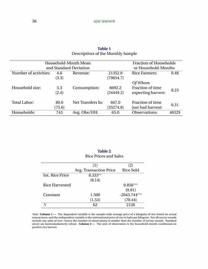
the seventy-two monthly rounds the project has released. Table 1 summarizes

the sample characteristics. I observe the average household for 65 months, but

have the full five years of data for over three-quarters of households. I observe

RISK AND ECONOMIC UNDER-SPECIALIZATION 13

each household in at least 45 months for over 95 percent of the sample. I call

households rice farmers if they harvest rice at any point in the sample, mak-

ing half the sample rice farmers. In any month a household expects a harvest

if it harvests rice in the next three months, and it had a recent harvest if it har-

vested rice in the current or previous three months. Table 1 shows households

expected a harvest one-fifth of the time. The number of economic activities is

the sum of the number of “large” businesses, crop-plots cultivated, types of live-

stock raised, number of jobs held by all members, number of miscellaneous or

small businesses, and an indicator for whether the household engages in aqua-

culture (raising fish or shrimp). Total revenue is the sum of revenue from each

economic activity and total consumption is all weekly and monthly household

expenditure. Net transfers, which I use to classify households as insured in Sec-

tion 6.1, are the total incoming transfers minus total outgoing transfers. I de-

flate revenue, consumption, and transfers to be in May 2007 Thai baht. I treat

a household-month surveyed in the first half of the month as though observed

in the previous month when I merge with time series data and define month

dummies. Since the rice price and consumer price index are monthly averages,

my convention best matches the survey response period to the horizons of the

aggregate prices.3 Table 1 shows the average monthly revenue is about 620 dol-

lars per month at May 2007 exchange rates. This seems high because revenue

is zero in many months and very high in others because of seasonality, as sug-

gested by the high standard deviation. Consumption is less seasonal and the

mean of 194 dollars is more reasonable.

I test the theory of lumpy investments with the annual panel. In addition

to the four provinces and roughly 1000 households followed from baseline, the

project added two more provinces and roughly 500 more households several

years into the survey (both from the new provinces and from the original vil-

lages to counter attrition). My final annual sample for the lumpy investment

tests is 1502 households. I construct the number of activities as closely as pos-

sible to my monthly measure: the sum of the number of large businesses, crop-

plots, jobs, herds, an indicator for aquaculture, and a subset of the miscella-

neous income sources. 4 The annual average of 4.6 activities is almost identical

3For more details on how I construct the variables, see Appendix A.4Miscellaneous income sources in the annual survey often include remittances and other

14 AJAY SHENOY

to the monthly average in Table 1, but it varies less because the annual measure

wipes out within-year variation in activities.

5 Suggestive Evidence of Risk and

Under-Specialization

If poor households avoid specialization to avoid risk their lives must have three

features: risky revenue, imperfect insurance, and a tendency to self-insure through

under-specialization. If any were missing I would find no response to risk in

later sections. But I examine a very special subpopulation—rice farmers expect-

ing a harvest—under very special circumstances. The subpopulation teaches

us about everyone else only if whatever drives their behavior affects everyone.

I show suggestive evidence that risk, poor insurance, and under-specialization

burden my entire sample.

5.1 Risky Revenue

Figure 3 shows the average coefficient of variation in monthly revenue when

I split my sample in four different ways: rice farmers versus non-rice farmers;

households with steady jobs versus those without; households with cash sav-

ings versus those without; and households in the top quartile of cash savings

versus everyone else. More precisely, I compute the coefficient of variation of

revenue for each household across all months where it meets or does not meet

the indicated criterion (e.g. holds a steady job). I then average the coefficients

across all households.

No one—not even a household where someone holds a steady job—has com-

pletely stable revenue. The households with steady jobs suffer revenue fluctua-

tions nearly as big as their average revenue, and those without steady jobs can

expect twice as much variation. Rice farmers not surprisingly suffer a much

sources that do not meet my definition of economic activities (namely, revenue generating ac-tivities that require labor). I filter these unwanted sources using regular expressions on the tex-tual descriptions of sources. The 1999 survey unfortunately does not contain textual descrip-tions, but the year dummies in the annual regressions should account for any 1999-specificmeasurement error.

RISK AND ECONOMIC UNDER-SPECIALIZATION 15

more variable stream of revenue than non-rice farmers. Finally, individuals

with large savings enjoy less variation in revenue, possibly because only house-

holds with stable revenue can accumulate savings.

5.2 Imperfect Insurance

Figure 4 graphs the top seven spontaneous responses to “What did your house-

hold do in the worst year [for income] of the last five to get by?” The most pop-

ular response was to take on an extra occupation, followed by working harder

than usual. These responses do not prove households avoid risk through under-

specialization, only that they cope with shocks through under-specialization.

But if households smooth their consumption by working more they must have

no better option. Borrowing money is only the third most popular response and

using savings only the fifth. The fourth most popular response is to consume

less, meaning many households lack even second-rate insurance.

Figure 5 gives direct evidence of bad insurance: the correlation between rev-

enue and consumption. I compute the correlation between monthly revenue

and consumption expenditure for each household over however many months

I observe it (72 months for the majority). If a risk-averse household has per-

fect insurance, its consumption should be independent of its current revenue;

in fact, it should be constant. A household without perfect insurance cuts con-

sumption when revenue falls, making the correlation positive. A higher correla-

tion is evidence of less insurance. The figure plots the density of the correlation

among rice farmers and non-rice farmers. Since zero is modal it appears many

households do have near-perfect insurance, but many more do not. The distri-

bution is heavily skewed towards less insurance with rice farmers particularly

uninsured.5 Some households have a negative correlation because of sampling

error: the true correlation might be zero, but my estimate fluctuates around the

truth and lands below zero for some households.

5The result may seem at odds with the high degree of insurance Townsend (1994) finds,but recall his result is that household consumption moves only with village-level and nothousehold-level income. Figure 5 does not control for village-level shocks because a house-hold cares only about having stable consumption, not where instability comes from. The shockI use for identification in Section 6 is a village-level shock: the international price of rice. Itis precisely the village’s inability to hedge against the price that drives households to under-specialize.

16 AJAY SHENOY

5.3 Risk and Under-Specialization

The theory predicts that rice farmers, who have riskier revenue and less insur-

ance, should have more economic activities than everyone else. The histogram

in Figure 6, which gives densities over the number of activities in an arbitrary

month, confirms that rice farmers are more likely to have a large number of

economic activities than everyone else. That said, very few households even

among non-rice farmers are perfectly specialized.

The last and simplest test is whether households with riskier revenue have

more activities. I average the number of activities and take the standard de-

viation of revenue for each household for all the months I observe it. Figure

7 plots the average number of economic activities against the log of the stan-

dard deviation after trimming the top and bottom 5 percent of standard devi-

ations. Households with riskier revenue tend to have more activities. A nice

scatterplot does not, of course, prove risk causes under-specialization. The

scatterplot only suggests the more rigorous results I report in Section 7.1 apply

beyond the subsample whose behavior gives identification. If all poor house-

holds have risky revenue, bad insurance, and the will to self-insure through

under-specialization, then my results might answer why all poor households

are under-specialized.

6 Causal Evidence of Risk and Under-Specialization

The ideal test for whether risk causes under-specialization is to randomize peo-

ple’s lives: make the returns to one group’s labor perfectly stable and another’s

very risky. The theory predicts people cursed with riskier lives will become jacks

of all trades while the lucky control group can specialize like Smith’s pin-maker.

Lacking the capacity and amorality to randomize risk into people’s lives, I

instead observe their responses to imminent changes in the riskiness of their

income. Changes in the monthly volatility of the international price of rice will

directly alter the variance of revenue for a household expecting a rice harvest.

By observing their responses I can isolate the effect of imminent income risk on

specialization.

RISK AND ECONOMIC UNDER-SPECIALIZATION 17

6.1 Estimating Risk Response

Changes in the international price of rice—and the responses they evoke in Thai

rice farmers—provide the exogenous variation in risk I need to test the model.

Between planting and harvest the price can change drastically, and anecdotal

evidence suggests farmers follow it closely in newspapers, radio broadcasts, and

television reports. Most of my sample grows the white rice that makes Thailand

the world’s biggest rice exporter, so the international price matters. 6 In Col-

umn 1 of Table 2 I report the correlation between the sample-wide average price

farmers receive and the international price. Though not perfect, the correlation

is significant and large enough to make following the international price worth

a farmer’s effort. If prices become more volatile the farmers know it and know

the value of their harvest has become riskier.

A response to volatility need not be a response to risky income unless it

comes from a specific group of farmers: those who harvest soon. Households

who do not farm rice respond to prices as consumers, and even comparing the

response of a rice farmer to someone who does not farm rice might just mea-

sure how rice farmers differ in their attitude to risk. Observing a household with

rice planted but not yet harvested—a farmer expecting a harvest in the next

three months —solves the problem of responses unrelated to income. Farmers

harvest rice roughly four months after planting and cannot hasten or delay the

date. Harvesting too soon yields immature grains while harvesting too late risks

losses to pests. The International Rice Research Institute states “the ideal har-

vest time lies between 130 and 136 days after sowing for late” varieties and gives

similarly narrow windows for other varieties (Gummert and Rickman, 2011).

Leaving rice on the stalk to wait out low prices is not an option. Although in

principle a farmer might store rice after harvesting, threshing, and drying, in

practice the farmers in my sample sell most of their rice as soon as they harvest

it. Colum 2 of Table 2 reports the correlation between how much rice a house-

hold sells and how much it harvests conditional on harvesting any during the

month. It suggests farmers sell almost every kilogram of rice immediately as it

6As expected, I find in unreported regressions that farmers harvesting only sticky rice havea lower response. The negative response too large to be the all-else-equal effect of growing ricethat will not be exported. Households who grow only sticky rice are unusual, their responsemay differ from that of other farmers for reasons beyond the type of rice.

18 AJAY SHENOY

comes from their fields. Households either cannot arbitrage—perhaps because

millers and other middlemen only buy at certain times—or they need cash too

desperately to wait.

The farmers in my sample are too small to affect the international price and

they cannot delay their harvest. After controlling for the responses of non-

rice farmers and rice farmers not expecting a harvest, any additional response

a farmer makes to higher volatility just before her harvest must be caused by

riskier income. Since I have a panel I can also control for household fixed-

effects to eliminate any fixed source of bias.7 The regression I run will actually

compare the farmer to herself at times when prices are volatile but she expects

no harvest, and times when she expects a harvest but prices are not volatile.

Figure 8 illustrates the specification.

When prices become volatile the farmer must decide whether to shift her

efforts away from maximizing the upcoming harvest. Figure 10 graphs the av-

erage household labor rice farmers devote to their fields in the months before

and after their harvest. Bringing a rice crop to harvest requires constant effort

right up through harvest, so working as a laborer or planting cassava detracts

from rice farming just like extra side activities detract from the primary activity

in the model.

To estimate the response I run the regression

[Activities]it = [FE]i + βM [Mean]t + βV [V olatility]t (1)

+ βE[Expecting Harvest]it + βH [Had Harvest]it

+ βRM [Rice Farmer]i × [Mean]t + βRV [Rice Farmer]i × [V olatility]t

+ βEM [Expecting Harvest]it × [Mean]t + βEV [Expecting Harvest]it × [V olatility]t

+ βHM [Had Harvest]it × [Mean]t + βHV [Had Harvest]it × [V olatility]t + εit.

Aside from the responses of non-farmers and farmers with no upcoming

harvest, I must also control for the responses of farmers who just had a har-

7For example, suppose only rich farmers plant in January to harvest in April. If the rice pricealways turns volatile in March, I might just estimate the effect of being a rich farmer. If seasonalselection and seasonal volatility matter, fixed-effects will deal with them.

RISK AND ECONOMIC UNDER-SPECIALIZATION 19

vest because it is negatively correlated with having an upcoming harvest and

cannot be left in the error term. In most of the results of Section 7.1 I replace

the main effects [Mean] and [Volatility] with month dummies. Month dummies

eliminate much of the variation but produce more conservative estimates.

The coefficient βEV on [ExpectingHarvest] × [V olatility] measures the aver-

age response to volatility of a farmer who expects a harvest, while controlling for

the responses of non-farmers and farmers without upcoming harvests. Since

the number of activities is my measure of specialization, that coefficient mea-

sures the causal effect of risk on under-specialization. Test 1 predicts it should

be positive. The coefficient βEM on [ExpectingHarvest] × [Mean] measures the

response to higher average prices, and Test 3 predicts it should be negative.

Test 2—that households with insurance should respond less to volatility—

requires a measure of insurance. In poor countries a household often relies on

family and friends for support in hard times. 8 Figure 11 shows the rice farmers

in my sample are no different: when the international price is low rice farm-

ers tend to receive more transfers. I calculate for each household the monthly

correlation between its net incoming transfers and its revenue, and call a house-

hold “insured” if that correlation is negative. I run (1) for both the insured and

uninsured sample. Test 2 predicts the risk response should be smaller among

the uninsured. I also run a version of (1) with additional interactions between

every variable and the indicator for being insured. Test 2 predicts the coeffi-

cient on the interaction between [ExpectingHarvest] × [V olatility] and insur-

ance should be negative. Insurance, however, is not exogenous and finding

the negative coefficient is only evidence consistent with the model. I cannot

rule out that households with insurance are different and respond differently to

volatility, so I cannot test the prediction as cleanly as I test the average response

to volatility and returns.

8Rosenzweig (1988) found that households structure themselves to ease income sharing.Townsend (1994) and more recently Munshi and Rosenzweig (2009) find village and caste net-works provide insurance in India. Yang and Choi (2007) show that rural Filipino householdswho suffer bad rainfall shocks receive more remittances from overseas family.

20 AJAY SHENOY

6.2 A Monthly Measure of Conditional Rice Price Volatility

The theory predicts an increase in the variance of a household’s income should

cause it to enter more side activities. Since I examine rice farmers expecting a

harvest I need a monthly measure of the volatility of prices. No standard mea-

sure of rice price volatility exists so I construct my own from the time series

of prices. I model the monthly price with the Autoregressive Conditional Het-

eroskedasticity (ARCH) model of Engle (1982) with one modification: I assume

the level of the price follows a random walk. The assumption reduces the num-

ber of parameters I must estimate and, as I show below, matches the true series

well.

More formally, suppose Pt is the price in month t and zt is an orthogonal

standard normal innovation. The model is

Pt = Pt−1 + εt

εt = zt√ht, zt ∼ N(0, 1)

ht = τ0 + τ1ε2t−1.

I estimate the model using conditional maximum likelihood.9 Suppose a

farmer must choose his activities at the beginning of the month before the ac-

tual price is known. He will base his decision on the conditional mean E[Pt |Pt−1] = Pt−1 and the conditional variance E[σ2

t | ε2t−1] = ht. The predicted value

h is a consistent estimate of the true conditional variance, so I use its square

root√h (the conditional standard deviation) as my measure of volatility.

Figure 9 plots the actual price of rice, the predicted mean, and the predicted

standard deviation. Simple though it is, the random walk assumption makes

very accurate predictions about the mean: a regression of price on its lag gives a

coefficient of .995. The red lines demarcate the start and end of the time period

covered in the monthly panel data. The sample spans a time when prices are

relatively stable, ending well before the massive food price spike of 2008.

The econometrically-minded may worry if regressions on a regressor gener-

ated from a time series model are consistent. Pagan (1984) confirms that the

9The true distribution of zt need not be normal; the (quasi) maximum likelihood estimatorbased on a normal distribution is still consistent.

RISK AND ECONOMIC UNDER-SPECIALIZATION 21

ARCH predicted value (though not the residual) will give consistent estimates,

and I have confirmed in monte carlo simulations that panel estimators are con-

sistent as well. Since the volatility is generated I use a two-stage bootstrap for

all inference in the results I report in Section 7.1. The details of the bootstrap

are in the Online Appendix C.

6.3 The Costs of Under-Specialization

Risk may drive households into extra side activities, but are they costly? It is

hard to imagine why else the household would diversify only when risk increases.

If the extra activities were costless the household ought to max out its activities

at all times regardless of movements in volatility. Test 4, however, suggests a di-

rect approach: to check whether revenue from side activities falls as the farmer

adds more activities.

Rises in price volatility will cause rice farmers expecting a harvest to increase

their number of activities, but by construction these farmers have not yet sold

their harvest and collected their primary revenue. I cannot say anything about

their total revenue because all they have collected is their revenue from side

activities. Test 4 solves the problem because it says revenue from side activi-

ties can fall when the household adds even more activities, and a fall in side

revenue is sufficient to conclude under-specialization is costly. Figure 6 shows

that most rice farmers have many activities—cassava fields or bakeries—even

when volatility is average. Test 4 says that if a rice farmer’s revenue from cas-

sava falls when he starts working as a casual laborer, and the loss to cassava

outweighs the gain from wages, then extra activities are costly. I can confirm

extra activities are costly if I have instruments that drive farmers into more ac-

tivities without directly affecting revenue.

The response of farmers expecting a harvest to the mean and volatility of

prices is exactly the instrument I need. Since household revenue before the

harvest does not include revenue from rice, movements in the rice price cannot

affect revenue directly. Greater risk might cause a household to invest less in

physical and human capital, but the effect will not appear for years to come.

My regressions measure very short run changes from month-to-month. I can

then run the following first-stage regression

22 AJAY SHENOY

[Activities]it = [FE]i +∑m

βD,m[Month Dummy] (2)

+ βE[Expecting Harvest]it + βH [Had Harvest]it

+ βRM [Rice Farmer]i × [Mean]t + βRV [Rice Farmer]i × [V olatility]t

+ βEM [Expecting Harvest]it × [Mean]t + βEV [Expecting Harvest]it × [V olatility]t

+ βHM [Had Harvest]it × [Mean]t + βHV [Had Harvest]it × [V olatility]t + εit.

and use [ExpectingHarvest] × [Mean] and [ExpectingHarvest] × [V olatility]

as excluded instruments for [Activities] the second-stage regression

[Revenue]it = [FE]i + γA [Activities]it +∑t

γD,m[Month Dummy]t (3)

+ γE[Expecting Harvest]it + γH [Had Harvest]it

+ γRM [Rice Farmer]i × [Mean]t + γRV [Rice Farmer]i × [V olatility]t

+ γHM [Had Harvest]it × [Mean]t + γHV [Had Harvest]it × [V olatility]t + uit.

Test 4 predicts the coefficient on [Activities] should be negative. The final

test, Test 5, predicts the coefficient on [Activities] in the simple OLS regression

[Revenue]it = κA[Activities]it +∑t

κD,m[Month Dummy]t + εit (4)

should be biased upward relative to the IV regression because the house-

holds with more activities are also the households who pay lower costs for them.

7 Risk and Under-Specialization Results

RISK AND ECONOMIC UNDER-SPECIALIZATION 23

7.1 Main Results

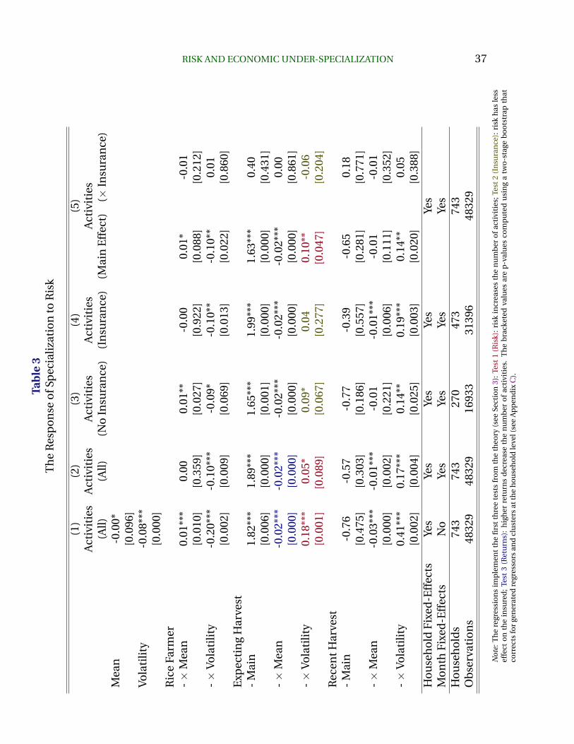
Table 3 reports the response of specialization to risk estimated with variations

of (1). Table 4 reports the effect of under-specialization on revenue estimated

with (3) and (4). All regressions except simple OLS in Column 1 of Table 4 use

the generated measure of volatility, so I calculate the p-values and confidence

intervals of all regressions using a two-stage bootstrap. The bootstrap, which

I describe in detail in the online appendix, corrects for the generated volatility

measure and within-household correlation in the error term across time.

The model’s first prediction—Test 1—is that riskier revenue causes entry

into more activities. The effect of risk on activities is the coefficient on [ExpectingHarvest]×[V olatility] in Column 1 of Table 3, and as predicted it is positive and significant.

The model also predicts in Test 3 that higher expected returns to the primary

activity (rice farming) should cause a decrease in activities. The coefficient on

[ExpectingHarvest] × [Mean] confirms that higher returns have a negative and

significant effect on number of activities. Column 2 verifies that both results

hold when I include month fixed-effects.

Test 2 says households with insurance will respond less strongly to risk than

households without insurance. Columns 3 and 4 measure the effect of risk

on under-specialization separately in the sub-samples without and with insur-

ance. As predicted, the coefficient on [ExpectingHarvest]×[V olatility] is smaller

and insignificant among the insured households. Column 5 estimates a single

regression on the entire sample with full interactions with the indicator for in-

surance. The main effect of [ExpectingHarvest]× [V olatility] captures the effect

of risk on uninsured households, and it remains positive and significant. As the

model predicts, the coefficient on [ExpectingHarvest]×[V olatility]×[Insurance]

is negative, though not significant. This may be because the correction for gen-

erated regressors reduces the power of my hypothesis tests.

The average expected price and volatility for all available months is 137.4

and 8.8 (the averages within range of the panel are similar). At the mean the

estimates imply a 10 percent increase in volatility causes the average rice farmer

to enter an extra 0.04 activities and the uninsured farmer to enter 0.08 activities.

The average elasticity for everyone and uninsured rice farmers is 0.09 and 0.18.

For comparison a 10 percent increase in the expected price causes a decrease of

24 AJAY SHENOY

0.26 activities and an elasticity of -0.6. In other words, a 10 percent increase in

volatility lowers specialization among uninsured farmers as much as a 3 percent

decrease in the average price.

Test 4 states that if the extra activities rice farmers take on cause their rev-

enue to fall, then the failure to specialize is costly. I implement it by running (2)

as a first-stage regression for (3), which instruments number of activities with

the response to price mean and volatility of farmers expecting a harvest. Col-

umn 2 of Table 4 reports the two-stage least squares coefficient on [Activities]

is negative and significant, confirming that under-specialization is costly. Col-

umn 1 reports the results of the simple OLS regression with month dummies of

revenue on number of activities (4). Test 5 says the OLS coefficient on [Activities]

should be biased positively relative to the two-stage least squares coefficient

because the farmers with more activities are the ones who pay lower costs for

each. The OLS coefficient is biased so strongly the sign flips: naive OLS makes

under-specialization seem wonderful.

Do not take the two-stage least squares coefficient as the average cost of

extra activities. A household does not, as it implies, give up more than half its

monthly revenue for each extra activity. Recall from the model in Section 3 that

when the mean and volatility of returns change they move the thresholds that

determine how high a cost households are willing to pay to enter additional

activities. When the volatility rises the households who enter more activities are

the ones with higher-than-average costs—the households who must be dragged

kicking and screaming into side activities. The coefficient is not the average cost

but a local average cost analogous to the local average treatment effect (Angrist

et al., 1996). Although its negative and significant sign confirms the model’s

predictions the coefficient does not map to anything with an easy economic

interpretation.

7.2 Robustness

Is it possible that risk causes households to work more and put the extra labor

towards more activities? If so, the simple logic of the model—that households

must deprive their primary activity of labor to start side activities—becomes

murkier. Column 1 of Table 13 reports that controlling for total household labor

RISK AND ECONOMIC UNDER-SPECIALIZATION 25

does not change the main result. Column 2 settles a similar concern: that risk

might cause households to recall migrants and use the extra household mem-

bers to work at additional activities. Controlling for the number of members

in the household (defined as having slept there in the past few weeks) does

not change the risk response results. Column 3 confirms neither issue affects

the second-stage results—that additional activities cause lower side revenue—

either.

In results I leave for the online appendix I look for and reject several other

confounders. If returns across activities are not independent—that is, the vari-

ance of rice prices affects the price of corn or cassava—I might mistake substi-

tution towards better outside options for under-specialization due to risk. In

principle I control for this by controlling for the response of rice farmers not

expecting a harvest (the substitution effect is no weaker for them), but I also

check for it directly. I find that excluding crop-plots from my measure of activ-

ities does not change the qualitative result. I still see activities have a negative

effect on side revenue when I exclude revenue from all crops. I also regress vil-

lage median wages on within-village averages of all the variables in (1) and find

nothing. One last worry is that households may actually respond when prices

change because they must revise their expectations of their permanent income.

Then the true driver of the response I see is the simple change in price levels,

which is correlated with the predicted volatility. I replace my volatility measure

with the simple change in prices to confirm it does not affect the number of

activities.

The skeptical reader may wonder if Thai rice farmers estimate ARCH mod-

els before deciding how to live. The ARCH only formalizes a simple intuition:

when prices fluctuate wildly it means they are risky. I confirm in the online ap-

pendix that simpler measures of the mean and volatility—the current price and

the absolute change in the price since last month—produce similar results.

8 The Alternative Theory: Lumpy Investments

If “the poor cannot raise the capital they would need to run a business that

would occupy them fully” (Banerjee and Duflo, 2007), households cannot spe-

26 AJAY SHENOY

cialize. Suppose a man can be a tailor, a carpenter, or a baker. He can learn

to sew or bake but cannot can sew more than a few shirts or bake more than

a few loaves without a sewing machine or oven. He lacks the cash or credit for

either. Since his bakery remains too small to support his family he must also

tailor, and the tailor next door must bake bread. Both would rather specialize

and trade but lack the capital.10

To test the lumpy investment theory I exploit a government program that

produced quasi-experimental variation in credit availability. If the theory is

true, households would specialize if only they had the credit to make the neces-

sary lumpy investment. Then we would expect a relaxation of credit constraints

would cause a decrease in each household’s number of economic activities. The

program I exploit is the Million Baht Program. The program was rapidly imple-

mented in all the villages of the Townsend Thai annual survey (among others)

in the latter part of 2001 and provided one million Thai baht to each village’s

community lending facility. Since the size of the transfer was the same for each

village regardless of size, a smaller village received a larger per-household trans-

fer. Kaboski and Townsend (2009, 2011), who are the first to exploit the program,

argue that villages in Thailand were delineated decades prior to the program

by bureaucratic fiat for administrative convenience. Since the sizes of villages

are effectively random, the per-household increase in credit availability is also

random. The authors find the program had little effect on average investment

largely because decreased investment by some households offset the increased

investment by others. More recently, Shenoy (2013) used the program to mea-

sure the effect of credit on production misallocation in rice farming. I find the

program had significant but small effects on misallocation caused by financial

market failures.11

10The inability to invest may create another source of under-specialization: the need to takeon extra jobs because one may only work so long at any single task. Suppose labor and cap-ital are complements, and make it simple with an extreme example: perfect complementar-ity. Suppose an activity m produces revenue with production function ym = Am min[L,K],with m = T,B for tailoring or baking. Suppose AT > AB for some household. If the house-hold’s labor endowment is L, it will specialize in tailoring with K∗ = L. But suppose increas-ing capital beyond K < K∗ requires a lumpy investment the household cannot afford. If thehousehold specialized, it would be left with L − K units of unused labor. In other words, itwould be idle. The alternative is to spend its remaining time baking, so its total revenue isAT K + AB(L− K) < AT L.

11Is the program still a valid source of exogenous variation if it affected within-sector effi-

RISK AND ECONOMIC UNDER-SPECIALIZATION 27

Since I do not know the exact month when the program reached any given

village, I use the annual data and treat 2001 as the year of program implemen-

tation. The program effect is captured by the interaction of the year of (and

year after) implementation interacted with some measure of village size. In one

specification I use an indicator for whether the household is in the bottom quar-

tile in number of households; in the other I use the actual per-household injec-

tion (1 million/number of households). The lumpy investment theory predicts

the signs of the coefficients should be negative and significant.

Table 5 reports that the coefficients have the wrong sign. The positive coef-

ficients on 2001 × Small and the other interactions are not consistent with the

lumpy investment theory, but might be consistent with the model from Sec-

tion 3. If risk is really what drives under-specialization and some households

want more economic activities but cannot afford to pay the fixed-cost, pro-

viding cheap financing might increase the number of activities. But this story,

which lacks direct evidence and rests on coefficients that are largely not signfi-

cant, remains only a story. Only the coefficient on 2002×Credit/HH in Column

2 is (marginally) significant, and even that significance vanishes when I restrict

the estimation in Column 4 to a balanced panel.

My results do not mean credit constraints have no effect on specialization.

Aside from the usual caveats—a lack of evidence is not a rejection, and rejec-

tion in Thailand does not mean rejection in other countries—I only test a lim-

ited form of the theory. The smallest villages received per-household credit in-

jections of half the median income. If households literally need sewing ma-

chines and ovens the credit injection would cover it, and the story that small

entrepreurs need small loans is the premise of most micro credit charities. But if

a few households want to build factories that would provide stable and salaried

jobs to everyone else, the Million Baht Program is too small.

ciency? Improved within-sector efficiency would likely increase the returns to any particularactivity and so should increase the incentives to specialize. If anything, my estimates should bebiased towards finding an effect, making the lack of evidence that much more pronounced.

28 AJAY SHENOY

9 Conclusion

If the benefits of specialization are so remarkable, why do the poor fail to exploit

them? One reason is fear: the fear of specializing in an activity with risky re-

turns. I find that Thai rice farmers expecting a harvest increase their number of

economic activities when confronted with more volatile prices, which is exactly

what a simple model of risk and under-specialization predicts. I find sugges-

tive evidence that risk affects uninsured households the most and confirm the

model’s prediction that higher expected returns lower the number of activities.

The size of an uninsured household’s response to a 10 percent fall in volatility is

equivalent to a 3 percent rise in expected returns. I use the exogenous change

in the number of activities to verify under-specialization costs households rev-

enue. Finally, I test an alternative theory of under-specialization—that the poor

run many small businesses because they cannot afford the lumpy investments

needed to grow any one to a viable size—and find no supporting evidence.

The pin-maker wastes time when he switches from straightening wires to

cutting them, and I find evidence of this waste in rural Thailand. My results

do not measure the talent and investment wasted when the poor forego exper-

tise in a single trade or investment in a single business. This kind of under-

specialization, which changes the structure of an economy, is a long run phe-

nomenon that requires a long run analysis. Future research must study whether

long run risk causes long run under-specialization and how much it costs.

References

Angrist, J. D., Imbens, G. W., and Rubin, D. B. (1996). Identification of Causal

Effects Using Instrumental Variables. Journal of the American Statistical

Association, 91(434):444–455.

Bandyopadhyay, S. and Skoufias, E. (2012). Rainfall Variability, Occupational

Choice, and Welfare in Rural Bangladesh. World Bank Policy Research

Working Paper, (6134).

Banerjee, A. and Duflo, E. (2007). The Economic Lives of the Poor. The Journal

RISK AND ECONOMIC UNDER-SPECIALIZATION 29

of Economic Perspectives: A Journal of the American Economic Association,

21(1):141.

Engle, R. (1982). Autoregressive Conditional Heteroscedasticity with Estimates

of the Variance of United Kingdom Inflation. Econometrica: Journal of the

Econometric Society, pages 987–1007.

Gummert, M. and Rickman, J. (2011). When to Harvest. Technical report, Inter-

national Rice Research Institute.

Jacoby, H. G. and Skoufias, E. (1997). Risk, Financial Markets, and Human Capi-

tal in a Developing Country. The Review of Economic Studies, 64(3):311–335.

Kaboski, J. and Townsend, R. (2009). The Impacts of Credit on Village

Economies. MIT Department of Economics Working Paper No. 09-13.

Kaboski, J. and Townsend, R. (2011). A Structural Evaluation of a Large-Scale

Quasi-Experimental Microfinance Initiative. Econometrica, 79(5):1357–

1406.

Menon, N. (2009). Rainfall Uncertainty and Occupational Choice in Agricultural

Households of Rural Nepal. The Journal of Development Studies, 45(6):864–

888.

Munshi, K. and Rosenzweig, M. (2009). Why Is Mobility in India So Low? Social

Insurance, Inequality, and Growth. Technical report, National Bureau of

Economic Research.

Murphy, K. and Topel, R. (2002). Estimation and Inference in Two-Step Econo-

metric Models. Journal of Business & Economic Statistics, 20(1):88–97.

Pagan, A. (1984). Econometric Issues in the Analysis of Regressions with Gener-

ated Regressors. International Economic Review, 25(1):221–247.

Rosenzweig, M. and Binswanger, H. (1993). Wealth, Weather Risk and the Com-

position and Profitability of Agricultural Investments. The Economic Jour-

nal, 103(416):56–78.

Rosenzweig, M. R. (1988). Risk, Implicit Contracts and the Family in Rural Areas

of Low-Income Countries. The Economic Journal, 98(393):1148–1170.

30 AJAY SHENOY

Shenoy, A. (2013). Market Failures and Misallocation: Decomposing Factor Mis-

allocation by Source.

Townsend, R. (1994). Risk and Insurance in Village India. Econometrica: Journal

of the Econometric Society, pages 539–591.

Townsend, R., Paulson, A., Sakuntasathien, S., Lee, T. J., and Binford, M. (1997).

Questionnaire Design and Data Collection for NICHD Grant Risk, Insur-

ance and the Family and NSF Grants.

Townsend, R. M. (2012). Townsend Thai Project Monthly Survey (1-60) Initial

Release. Murray Research Archive [Distributor] V1 [Version].

Yang, D. and Choi, H. (2007). Are Remittances Insurance? Evidence from Rain-

fall Shocks in the Philippines. The World Bank Economic Review, 21(2):219–

248.

RISK AND ECONOMIC UNDER-SPECIALIZATION 31

A Detailed Data Appendix

A.1 Time Series Variables

• Consumer Prices: From Bank of Thailand monthly index, acquired from

Global Financial Data database. Data were used with permission of Global

Financial Data.

• International Rice Price: Acquired from IMF monthly commodity price

data. Deflated using monthly consumer price index.

A.2 Panel Variables

• Rice Harvest: From module 7 (Crop Harvest) section of the monthly sur-

vey. Keep only un-milled rice (both sticky and non-sticky). Define rice

harvest soon as a reported positive harvest of unmilled rice in the subse-

quent three months. Define rice harvest past as having had positive har-

vest of unmilled rice in the current or previous three months. Define rice

farmer (or rice harvest ever) as having had a positive rice harvest at any

point in the survey span.

• Crop-Plots: From module 5 (Crop Activities) section of the monthly sur-

vey. Make the monthly aggregate of “value transacted” for each house-

holds sale of each crop. This is the revenue from crops. For number of

crop plots, I use the “projected harvest” table, which asks farmers to pre-

dict revenue for each productive crop. Every entry corresponds to a dif-

ferent perceived revenue stream for the farmer, so I take number of crop-

plots as simply the count of these for each household in each month.

• Aquaculture: From module 10 (Fish-Shrimp) of the monthly survey. For

each household, make monthly aggregates of the value of fish and shrimp

output; this is the revenue from aquaculture. I compute whether a house-

hold does aquaculture as whether it reports raising fish/shrimp or having

shrimp ponds in a given month.

• Large Businesses: From module 12 (Household Business) of the monthly

survey. For each household, make monthly aggregates of the cash and in-

32 AJAY SHENOY

kind revenue plus the value of products/services consumed by the house-

hold; this is the revenue from large businesses. Compute the number of

businesses for each household as the number of entries in the household

report of revenues.

• Small/Miscellaneous Businesses: From module 24 (Income) of the monthly

survey. For each household, make monthly aggregates of the cash and

in-kind revenue for each “other” income source; this is the revenue from

miscellaneous businesses. Compute the number of miscellaneous activi-

ties for each household as the number of entries in the household report

of revenues.

• Number of Jobs: From module 11 (Activities-Occupation). For each per-

son and each job number in any month, mark if it was worked the pre-

vious two and the following two months (note that jobs are not assigned

job numbers in their first months, so technically I only check the previous

one month as it must have been worked the month before to have an ID).

If so, it is a “steady job.” I count each households total number of jobs and

steady jobs each month, then compute the number of unsteady jobs as

the difference. For each job and each month, sum the cash and in-kind

payments and aggregate by household-month. This is the monthly job

revenue.

• Number of Activities: I define number of activities as simply the sum of

the number of crop plots, the number of livestock activities, the indicator

for practice of aquaculture, the number of large businesses, the number

of jobs, and the number of miscellaneous activities.

• Total Revenue, Consumption, and Transfers: Total revenue is the sum of

revenue from crop activities, livestock activities, aquaculture, large busi-

nesses, jobs, and miscellaneous activities. Total consumption is the sum

of all domestic expenditures by both cash and credit plus consumption

of home-produced goods. Expenditures reported at a weekly rather than

monthly frequency (in module 23W, Weekly Expenditures Update) are ag-

gregated by month for each household and added to those reported at a

RISK AND ECONOMIC UNDER-SPECIALIZATION 33

monthly frequency (in module 23M, Monthly Expenditures Update). Trans-

fers are defined as the household’s net incoming transfers. More precisely,

I aggregate by household-month the transfers from people inside and out-

side the village and subtract similarly aggregated transfers to people in-

side and outside the village (all found in module 13 on Remittances). I use

only transfers not earmarked for a specific event because these unplanned

transfers are more like insurance.

B Verifying the Validity of Assumptions

C Inference: The Two-Stage Bootstrap

The predicted mean and volatility are both generated regressors, so I must ad-

just my inference to account for their presence. It is easy to see that under my

assumptions the full estimators match the conditions for Murphy and Topel

(2002). Directly applying their analytic expressions is inconvenient and also

problematic because small sample bias in the time series estimates might pro-

duce an abnormal small sample distribution for the estimated parameters. But

the asymptotic normality their propositions guarantee also ensures the validity

of bootstrapped confidence intervals and hypothesis tests.

I implement the procedure as outlined in Figures 12-14. First, I prepare the

time series of rice prices for resampling. I form “blocks” consisting of the con-

temporaneous price and however many lags I need to estimate the time series

model. I then group every observation into one or more “blocks of blocks,” con-

tiguous interlocking sets of observations and their associated lags.

Next, I run the bootstrap replications. Each replication follows five interme-

diate steps. First, I sample with replacement the blocks of blocks of rice prices to

construct a bootstrapped time series of equal length to the original time series.

I estimate the parameters of the time series model on the bootstrapped data.

I then resample with replacement households (together with all their monthly

observations) from the panel to construct a bootstrapped panel with as many

households as the original panel. Then I use the estimated time series model

to predict the conditional mean and variance of the international rice price for

34 AJAY SHENOY

each household-month observation. Finally, I estimate the panel specification

and record the resulting coefficients. I run 1000 replications for the risk specifi-

cation and 2000 replications for the IV specifications.

The final step is to compute confidence intervals and p-values. To construct

confidence intervals, I use the dataset of estimated parameters from bootstrap

replications to find the 2.5th and 97.5th percentiles. These are the boundaries

of the 95% confidence interval. To construct p-values, I compute the absolute

t-statistic centered around the original parameter estimate for each replica-

tion. The fraction of these absolute t-statistics that is greater than the original

t-statistic is the p-value.

D Other Tests of Robustness

E Alternative Model: Minimum Labor Inputs

Is it plausible that the kinds of activities a rice farmer can enter three months

before his harvest would, as my model assumes, have a lumpy fixed cost? Find-

ing casual labor or growing cassava may be easy if the farmer has already done

so every time prices turned volatile in the past. In this appendix I build a model

without fixed costs where risk still causes under-specialization. The prediction’s

robustness is why I emphasize that my model of risk and under-specialization

is not the model, but just a convenient tool to formalize the intuition.

Let the household’s utility function be as before and for simplicity consider

the case of choosing between perfect specialization and one side activity. The

household can costlessly enter a side activity but must allocate it at least L > 0

units of labor. The lower-bound on labor choice captures the idea that it is not

worth an employer’s time to hire a worker for only a few hours per week, so even

work that does not require paying a fixed cost does require a lumpy investment

of time. I need the lumpiness to make specialization optimal for some degree

of riskiness. Otherwise the household always has a side activity and only varies

how much it works on the side activity instead of whether it has one at all. I also

assume the average return to the side activity is strictly less than the average

return to the primary activity—that is, wp − ws = w+ > 0. The household faces

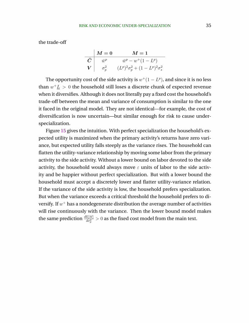
RISK AND ECONOMIC UNDER-SPECIALIZATION 35

the trade-off

M = 0 M = 1

C wp wp − w+(1− Lp)V σ2

p (Lp)2σ2p + (1− Lp)2σ2

s

The opportunity cost of the side activity is w+(1− Lp), and since it is no less

than w+L > 0 the household still loses a discrete chunk of expected revenue

when it diversifies. Although it does not literally pay a fixed cost the household’s

trade-off between the mean and variance of consumption is similar to the one

it faced in the original model. They are not identical—for example, the cost of

diversification is now uncertain—but similar enough for risk to cause under-

specialization.

Figure 15 gives the intuition. With perfect specialization the household’s ex-

pected utility is maximized when the primary activity’s returns have zero vari-

ance, but expected utility falls steeply as the variance rises. The household can

flatten the utility-variance relationship by moving some labor from the primary

activity to the side activity. Without a lower bound on labor devoted to the side

activity, the household would always move ε units of labor to the side activ-

ity and be happier without perfect specialization. But with a lower bound the

household must accept a discretely lower and flatter utility-variance relation.

If the variance of the side activity is low, the household prefers specialization.

But when the variance exceeds a critical threshold the household prefers to di-

versify. If w+ has a nondegenerate distribution the average number of activities

will rise continuously with the variance. Then the lower bound model makes

the same prediction dE[M ]dσ2p> 0 as the fixed cost model from the main text.

36 AJAY SHENOY

Table 1Descriptives of the Monthly Sample

Household-Month Mean Fraction of Householdsand Standard Deviation or Household-Months

Number of activities: 4.6 Revenue: 21352.8 Rice Farmers: 0.48(3.3) (79854.7)

Of WhomHousehold size: 5.3 Consumption: 6692.2 Fraction of time

0.23(2.4) (24449.2) expecting harvest:

Total Labor: 80.0 Net Transfers In: 667.0 Fraction of time0.31

(75.6) (35274.8) just had harvest:Households: 743 Avg. Obs/HH: 65.0 Observations: 48329

Table 2Rice Prices and Sales

(1) (2)Avg. Transaction Price Rice Sold

Int. Rice Price 0.333∗∗

(0.14)Rice Harvested 0.856∗∗∗

(0.01)Constant 1.500 -2043.744∗∗∗

(1.53) (70.44)N 62 2126

Note: Column 1 — The dependent variable is the sample-wide average price of a kilogram of rice based on actualtransactions, and the independent variable is the international price of rice in baht per kilogram. Not all survey roundsinclude any sales of rice—hence the number of observations is smaller than the number of survey rounds. Standarderrors are heteroskedasticity-robust. Column 2 — The unit of observation is the household-month conditional onpositive rice harvest.

RISK AND ECONOMIC UNDER-SPECIALIZATION 37

Tab

le3

Th

eR

esp

on

seo

fSp

ecia

lizat

ion

toR

isk

(1)

(2)

(3)

(4)

(5)

Act

ivit

ies

Act

ivit

ies

Act

ivit

ies

Act

ivit

ies

Act

ivit

ies

(All)

(All)

(No

Insu

ran

ce)

(In

sura

nce

)(M

ain

Eff

ect)

(×In

sura

nce

)M

ean

-0.0

0*[0

.096

]Vo

lati

lity

-0.0

8***

[0.0

00]

Ric

eFa

rmer

-×

Mea

n0.

01**

*0.

000.

01**

-0.0

00.

01*

-0.0

1[0

.010

][0

.359

][0

.027

][0

.922

][0

.088

][0

.212

]-×

Vola

tilit

y-0

.20*

**-0

.10*

**-0

.09*

-0.1

0**

-0.1

0**

0.01

[0.0

02]

[0.0

09]

[0.0

69]

[0.0

13]

[0.0

22]

[0.8

60]

Exp

ecti

ng

Har

vest

-M

ain

1.82

***

1.89

***

1.65

***

1.99

***

1.63

***

0.40

[0.0

06]

[0.0

00]

[0.0

01]

[0.0

00]

[0.0

00]

[0.4

31]

-×

Mea

n-0

.02*

**-0

.02*

**-0

.02*

**-0

.02*

**-0

.02*

**0.

00[0

.000

][0

.000

][0

.000

][0

.000

][0

.000

][0

.861

]-×

Vola

tilit

y0.

18**

*0.

05*

0.09

*0.

040.

10**

-0.0

6[0

.001

][0

.089

][0

.067

][0

.277

][0

.047

][0

.204

]R

ecen

tHar

vest

-M

ain

-0.7

6-0

.57

-0.7

7-0

.39

-0.6

50.

18[0

.475

][0

.303

][0

.186

][0

.557

][0

.281

][0

.771

]-×

Mea

n-0

.03*

**-0

.01*

**-0

.01

-0.0

1***

-0.0

1-0

.01

[0.0

00]

[0.0

02]

[0.2

21]

[0.0

06]

[0.1

11]

[0.3

52]

-×

Vola

tilit

y0.

41**

*0.

17**

*0.

14**

0.19

***

0.14

**0.

05[0

.002

][0

.004

][0

.025

][0

.003

][0

.020

][0

.388

]H

ou

seh

old

Fixe

d-E

ffec

tsYe

sYe

sYe

sYe

sYe

sM

on

thFi

xed

-Eff

ects

No

Yes

Yes

Yes

Yes

Ho

use

ho

lds

743

743

270

473

743

Ob

serv

atio

ns

4832

948

329

1693

331

396

4832

9

Not

e:T

he

regr

essi

on

sim

ple

men

tth

efi

rst

thre

ete

sts

fro

mth

eth

eory

(see

Sect

ion

3):

Test

1(R

isk)

:ri

skin

crea

ses

the

nu

mb

ero

fac

tivi

ties

;Tes

t2

(In

sura

nce

):ri

skh

asle

ssef

fect

on

the

insu

red

;Te

st3

(Ret

urn

s):

hig

her

retu

rns

dec

reas

eth

en

um

ber

of

acti

viti

es.

Th

eb

rack

eted

valu

esar

ep

-val

ues

com

pu

ted

usi

ng

atw

o-s

tage

bo

ots

trap

that

corr

ects

for

gen

erat

edre

gres

sors

and

clu

ster

sat

the

ho

use

ho

ldle

vel(

see

Ap

pen

dix

C).

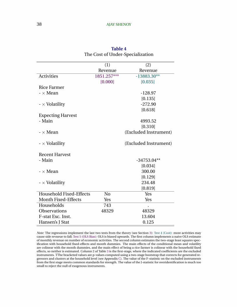
38 AJAY SHENOY

Table 4The Cost of Under-Specialization

(1) (2)Revenue Revenue

Activities 1851.257*** -13883.30**[0.000] [0.035]

Rice Farmer-×Mean -128.97

[0.135]-× Volatility -272.90

[0.618]Expecting Harvest- Main 4993.52

[0.310]-×Mean (Excluded Instrument)

-× Volatility (Excluded Instrument)

Recent Harvest- Main -34753.04**

[0.034]-×Mean 300.00

[0.129]-× Volatility 234.48

[0.819]Household Fixed-Effects No YesMonth Fixed-Effects Yes YesHouseholds 743 .Observations 48329 48329F-stat Exc. Inst. 13.604Hansen’s J Stat 0.125

Note: The regressions implement the last two tests from the theory (see Section 3): Test 4 (Cost): more activities maycause side revneue to fall; Test 5 (OLS Bias): OLS is biased upwards. The first column implements a naive OLS estimateof monthly revenue on number of economic activities. The second column estimates the two-stage least squares spec-ification with household fixed-effects and month dummies. The main effects of the conditional mean and volatilityare colinear with the month dummies, and the main effect of being a rice farmer is colinear with the household fixedeffects, so neither is estimated. Column 2 of Table 3 is the first-stage, where the indicated coefficients are the excludedinstruments. TThe bracketed values are p-values computed using a two-stage bootstrap that corrects for generated re-gressors and clusters at the household level (see Appendix C). The value of the F-statistic on the excluded instrumentsfrom the first stage meets common standards for strength. The value of the J-statistic for overidentification is much toosmall to reject the null of exogenous instruments.

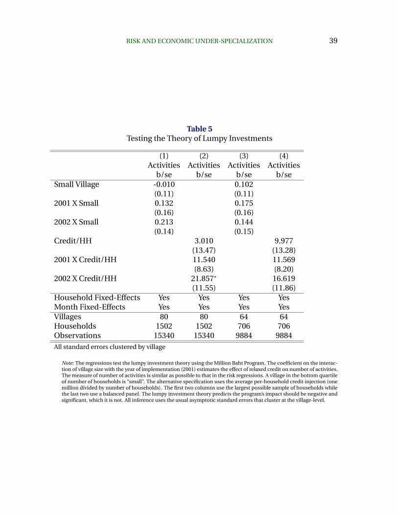
RISK AND ECONOMIC UNDER-SPECIALIZATION 39

Table 5Testing the Theory of Lumpy Investments

(1) (2) (3) (4)Activities Activities Activities Activities

b/se b/se b/se b/seSmall Village -0.010 0.102

(0.11) (0.11)2001 X Small 0.132 0.175

(0.16) (0.16)2002 X Small 0.213 0.144

(0.14) (0.15)Credit/HH 3.010 9.977

(13.47) (13.28)2001 X Credit/HH 11.540 11.569

(8.63) (8.20)2002 X Credit/HH 21.857∗ 16.619

(11.55) (11.86)Household Fixed-Effects Yes Yes Yes YesMonth Fixed-Effects Yes Yes Yes YesVillages 80 80 64 64Households 1502 1502 706 706Observations 15340 15340 9884 9884All standard errors clustered by village

Note: The regressions test the lumpy investment theory using the Million Baht Program. The coefficient on the interac-tion of village size with the year of implementation (2001) estimates the effect of relaxed credit on number of activities.The measure of number of activities is similar as possible to that in the risk regressions. A village in the bottom quartileof number of households is “small”. The alternative specification uses the average per-household credit injection (onemillion divided by number of households). The first two columns use the largest possible sample of households whilethe last two use a balanced panel. The lumpy investment theory predicts the program’s impact should be negative andsignificant, which it is not. All inference uses the usual asymptotic standard errors that cluster at the village-level.

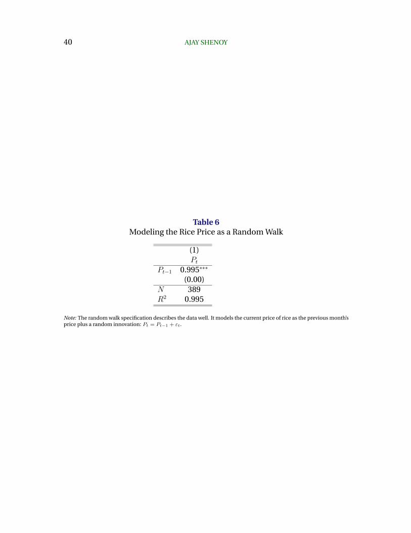
40 AJAY SHENOY

Table 6Modeling the Rice Price as a Random Walk

(1)Pt

Pt−1 0.995∗∗∗

(0.00)N 389R2 0.995

Note: The random walk specification describes the data well. It models the current price of rice as the previous month’sprice plus a random innovation: Pt = Pt−1 + εt.

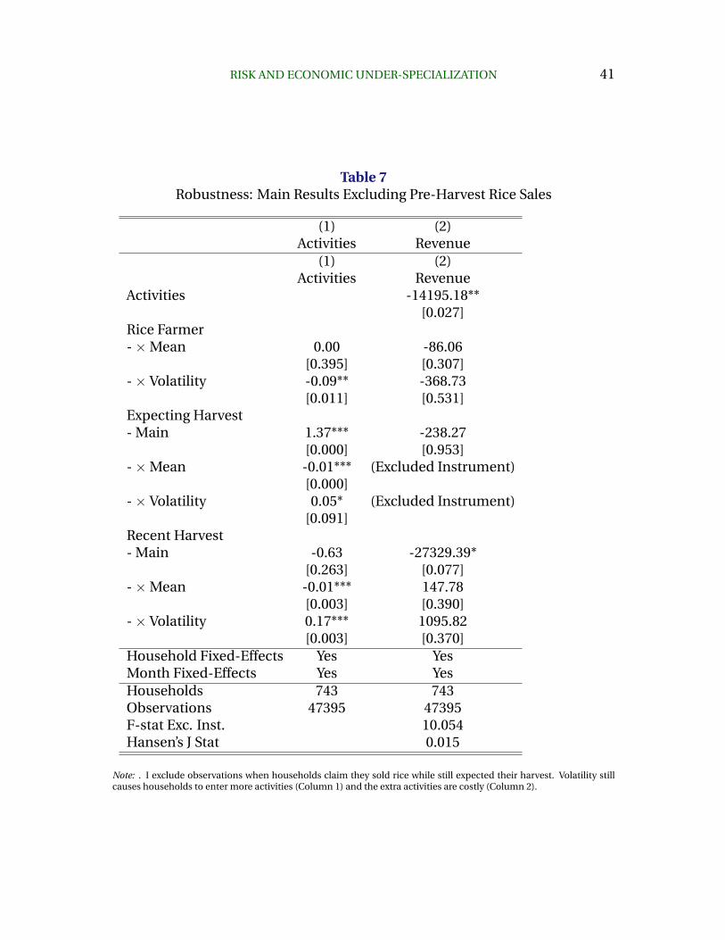
RISK AND ECONOMIC UNDER-SPECIALIZATION 41

Table 7Robustness: Main Results Excluding Pre-Harvest Rice Sales

(1) (2)Activities Revenue

(1) (2)Activities Revenue

Activities -14195.18**[0.027]

Rice Farmer-×Mean 0.00 -86.06

[0.395] [0.307]-× Volatility -0.09** -368.73

[0.011] [0.531]Expecting Harvest- Main 1.37*** -238.27

[0.000] [0.953]-×Mean -0.01*** (Excluded Instrument)

[0.000]-× Volatility 0.05* (Excluded Instrument)

[0.091]Recent Harvest- Main -0.63 -27329.39*

[0.263] [0.077]-×Mean -0.01*** 147.78

[0.003] [0.390]-× Volatility 0.17*** 1095.82

[0.003] [0.370]Household Fixed-Effects Yes YesMonth Fixed-Effects Yes YesHouseholds 743 743Observations 47395 47395F-stat Exc. Inst. 10.054Hansen’s J Stat 0.015

Note: . I exclude observations when households claim they sold rice while still expected their harvest. Volatility stillcauses households to enter more activities (Column 1) and the extra activities are costly (Column 2).

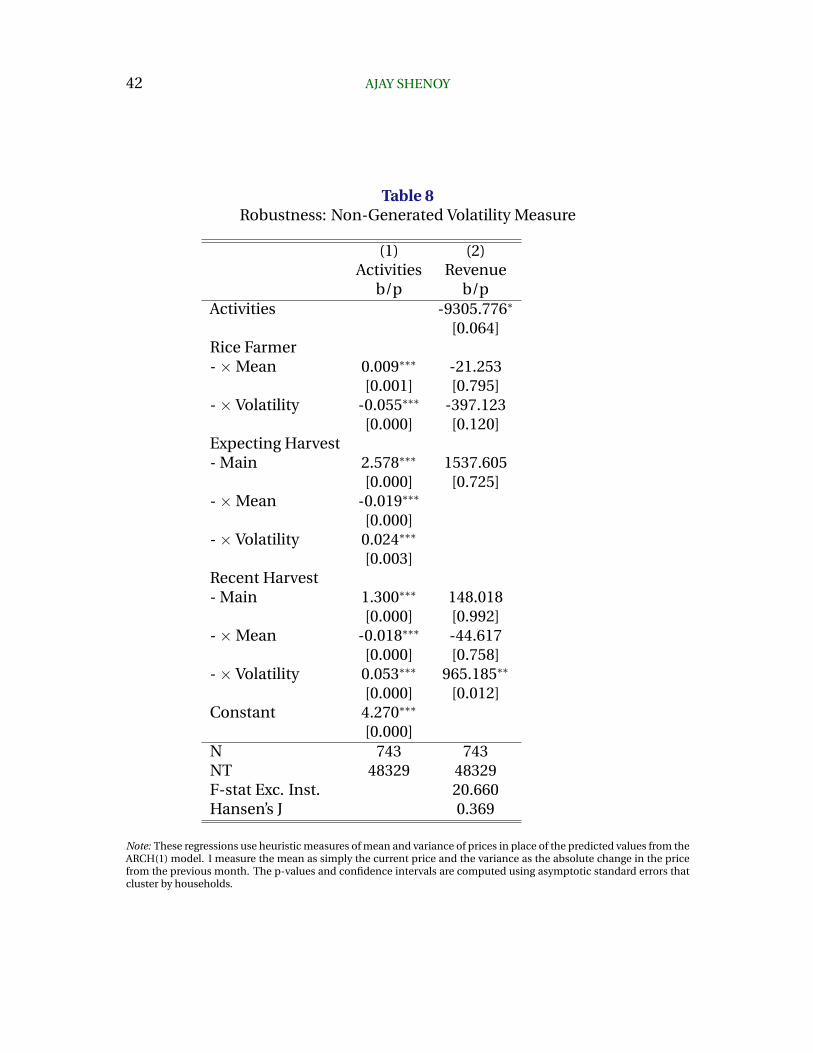
42 AJAY SHENOY

Table 8Robustness: Non-Generated Volatility Measure

(1) (2)Activities Revenue

b/p b/pActivities -9305.776∗

[0.064]Rice Farmer-×Mean 0.009∗∗∗ -21.253

[0.001] [0.795]-× Volatility -0.055∗∗∗ -397.123

[0.000] [0.120]Expecting Harvest- Main 2.578∗∗∗ 1537.605

[0.000] [0.725]-×Mean -0.019∗∗∗

[0.000]-× Volatility 0.024∗∗∗

[0.003]Recent Harvest- Main 1.300∗∗∗ 148.018

[0.000] [0.992]-×Mean -0.018∗∗∗ -44.617

[0.000] [0.758]-× Volatility 0.053∗∗∗ 965.185∗∗

[0.000] [0.012]Constant 4.270∗∗∗

[0.000]N 743 743NT 48329 48329F-stat Exc. Inst. 20.660Hansen’s J 0.369

Note: These regressions use heuristic measures of mean and variance of prices in place of the predicted values from theARCH(1) model. I measure the mean as simply the current price and the variance as the absolute change in the pricefrom the previous month. The p-values and confidence intervals are computed using asymptotic standard errors thatcluster by households.

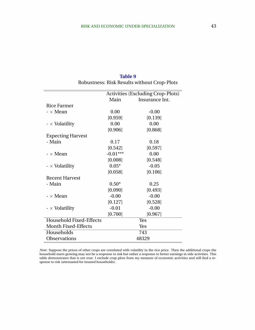
RISK AND ECONOMIC UNDER-SPECIALIZATION 43

Table 9Robustness: Risk Results without Crop-Plots

Activities (Excluding Crop-Plots)Main Insurance Int.

Rice Farmer-×Mean 0.00 -0.00

[0.959] [0.139]-× Volatility 0.00 0.00

[0.906] [0.868]Expecting Harvest- Main 0.17 0.18

[0.542] [0.597]-×Mean -0.01*** 0.00

[0.008] [0.548]-× Volatility 0.05* -0.05

[0.058] [0.106]Recent Harvest- Main 0.50* 0.25

[0.090] [0.493]-×Mean -0.00 -0.00

[0.127] [0.528]-× Volatility -0.01 -0.00

[0.700] [0.967]Household Fixed-Effects YesMonth Fixed-Effects YesHouseholds 743Observations 48329

Note: Suppose the prices of other crops are correlated with volatility in the rice price. Then the additional crops thehousehold starts growing may not be a response to risk but rather a response to better earnings in side activities. Thistable demonstrates that is not true: I exclude crop-plots from my measure of economic activities and still find a re-sponse to risk (attenuated for insured households).

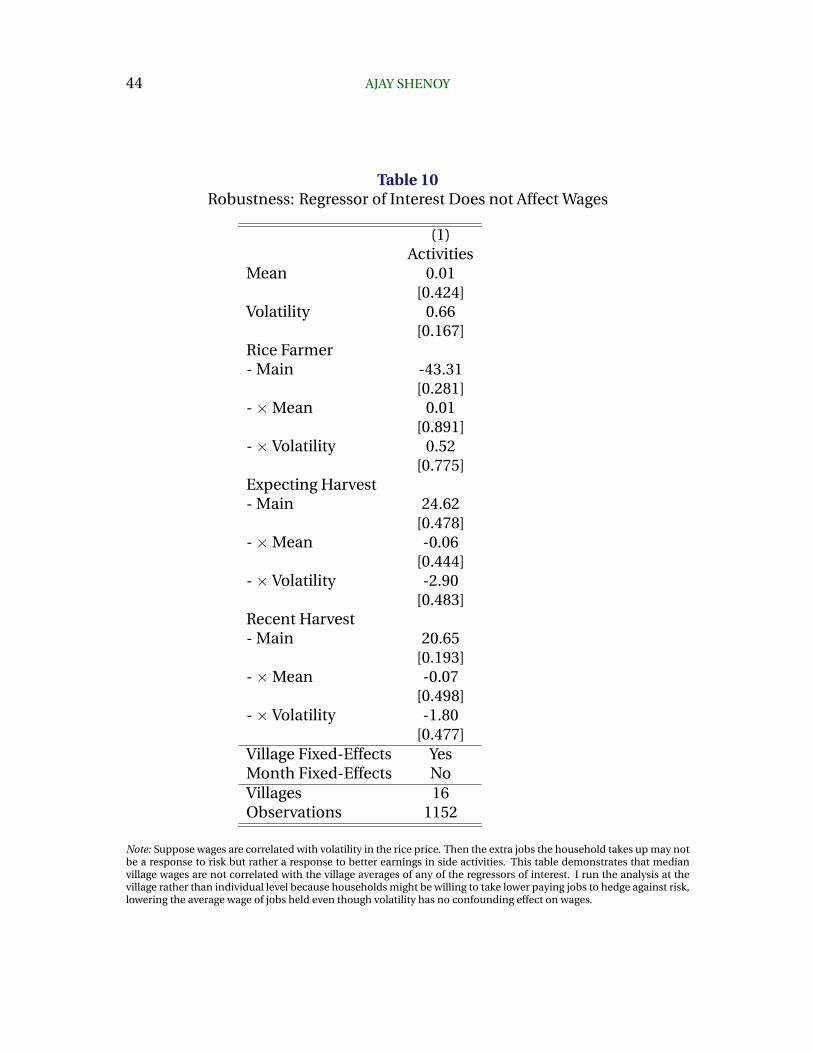
44 AJAY SHENOY

Table 10Robustness: Regressor of Interest Does not Affect Wages

(1)Activities

Mean 0.01[0.424]

Volatility 0.66[0.167]

Rice Farmer- Main -43.31

[0.281]-×Mean 0.01

[0.891]-× Volatility 0.52

[0.775]Expecting Harvest- Main 24.62

[0.478]-×Mean -0.06

[0.444]-× Volatility -2.90

[0.483]Recent Harvest- Main 20.65

[0.193]-×Mean -0.07

[0.498]-× Volatility -1.80

[0.477]Village Fixed-Effects YesMonth Fixed-Effects NoVillages 16Observations 1152

Note: Suppose wages are correlated with volatility in the rice price. Then the extra jobs the household takes up may notbe a response to risk but rather a response to better earnings in side activities. This table demonstrates that medianvillage wages are not correlated with the village averages of any of the regressors of interest. I run the analysis at thevillage rather than individual level because households might be willing to take lower paying jobs to hedge against risk,lowering the average wage of jobs held even though volatility has no confounding effect on wages.

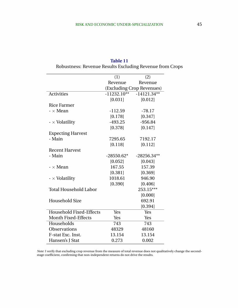
RISK AND ECONOMIC UNDER-SPECIALIZATION 45

Table 11Robustness: Revenue Results Excluding Revenue from Crops

(1) (2)Revenue Revenue

(Excluding Crop Revenues)Activities -11232.10** -14121.34**

[0.031] [0.012]Rice Farmer-×Mean -112.59 -78.17

[0.178] [0.347]-× Volatility -493.25 -956.84

[0.378] [0.147]Expecting Harvest- Main 7295.65 7192.17

[0.118] [0.112]Recent Harvest- Main -28550.62* -28256.34**

[0.052] [0.043]-×Mean 167.55 157.39

[0.381] [0.369]-× Volatility 1018.61 946.90

[0.390] [0.406]Total Household Labor 253.15***

[0.000]Household Size 692.91

[0.394]Household Fixed-Effects Yes YesMonth Fixed-Effects Yes YesHouseholds 743 743Observations 48329 48160F-stat Exc. Inst. 13.154 13.154Hansen’s J Stat 0.273 0.002

Note: I verify that excluding crop revenue from the measure of total revenue does not qualitatively change the second-stage coefficient, confirming that non-independent returns do not drive the results.

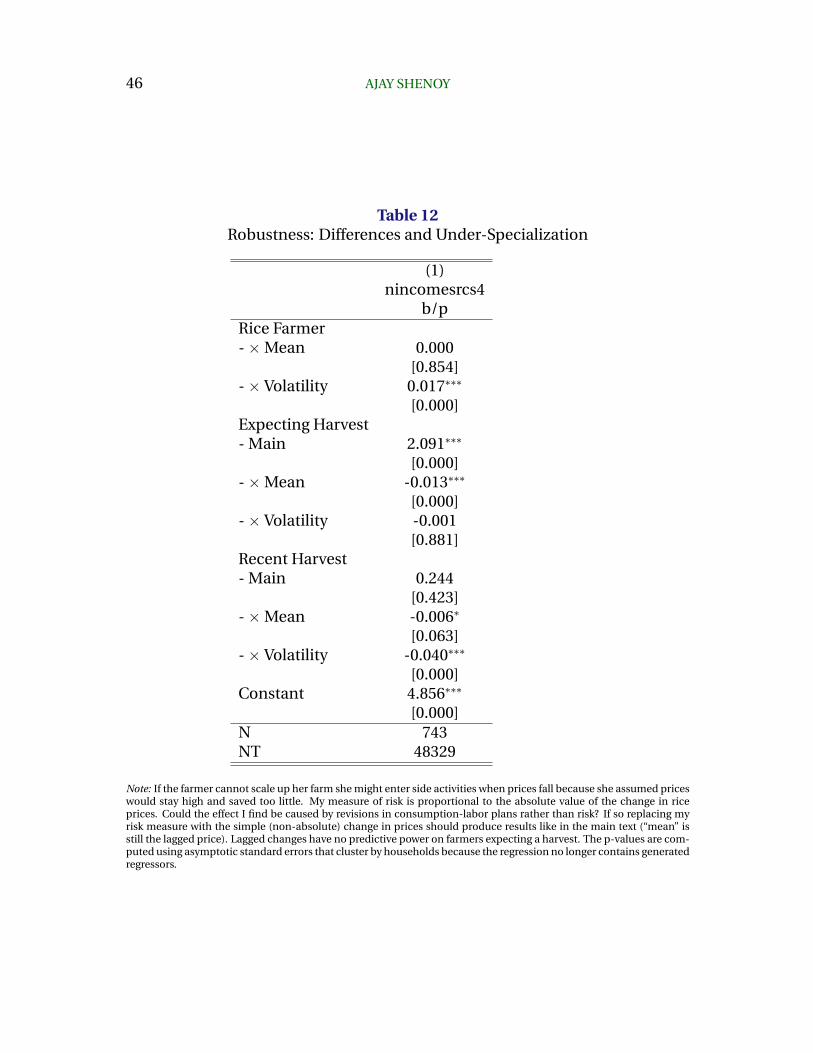
46 AJAY SHENOY

Table 12Robustness: Differences and Under-Specialization

(1)nincomesrcs4

b/pRice Farmer-×Mean 0.000

[0.854]-× Volatility 0.017∗∗∗

[0.000]Expecting Harvest- Main 2.091∗∗∗

[0.000]-×Mean -0.013∗∗∗

[0.000]-× Volatility -0.001

[0.881]Recent Harvest- Main 0.244

[0.423]-×Mean -0.006∗

[0.063]-× Volatility -0.040∗∗∗

[0.000]Constant 4.856∗∗∗

[0.000]N 743NT 48329

Note: If the farmer cannot scale up her farm she might enter side activities when prices fall because she assumed priceswould stay high and saved too little. My measure of risk is proportional to the absolute value of the change in riceprices. Could the effect I find be caused by revisions in consumption-labor plans rather than risk? If so replacing myrisk measure with the simple (non-absolute) change in prices should produce results like in the main text (“mean” isstill the lagged price). Lagged changes have no predictive power on farmers expecting a harvest. The p-values are com-puted using asymptotic standard errors that cluster by households because the regression no longer contains generatedregressors.

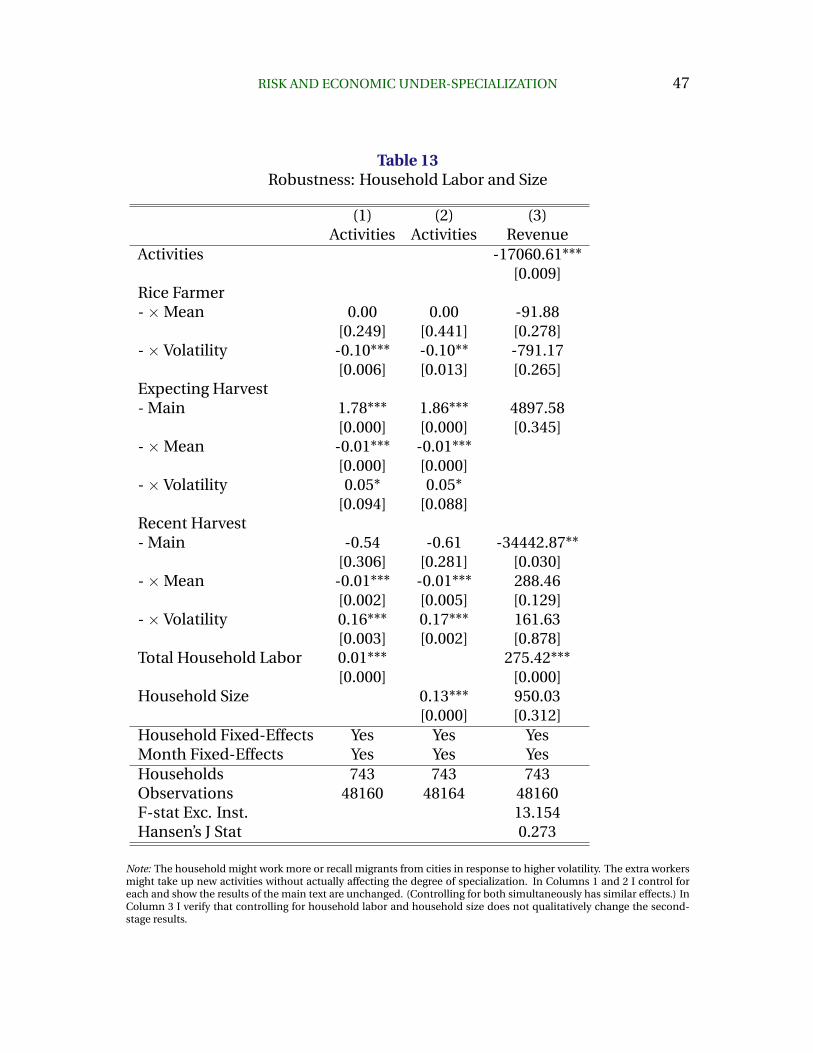
RISK AND ECONOMIC UNDER-SPECIALIZATION 47

Table 13Robustness: Household Labor and Size

(1) (2) (3)Activities Activities Revenue

Activities -17060.61***[0.009]

Rice Farmer-×Mean 0.00 0.00 -91.88

[0.249] [0.441] [0.278]-× Volatility -0.10*** -0.10** -791.17

[0.006] [0.013] [0.265]Expecting Harvest- Main 1.78*** 1.86*** 4897.58

[0.000] [0.000] [0.345]-×Mean -0.01*** -0.01***

[0.000] [0.000]-× Volatility 0.05* 0.05*

[0.094] [0.088]Recent Harvest- Main -0.54 -0.61 -34442.87**

[0.306] [0.281] [0.030]-×Mean -0.01*** -0.01*** 288.46

[0.002] [0.005] [0.129]-× Volatility 0.16*** 0.17*** 161.63

[0.003] [0.002] [0.878]Total Household Labor 0.01*** 275.42***

[0.000] [0.000]Household Size 0.13*** 950.03

[0.000] [0.312]Household Fixed-Effects Yes Yes YesMonth Fixed-Effects Yes Yes YesHouseholds 743 743 743Observations 48160 48164 48160F-stat Exc. Inst. 13.154Hansen’s J Stat 0.273

Note: The household might work more or recall migrants from cities in response to higher volatility. The extra workersmight take up new activities without actually affecting the degree of specialization. In Columns 1 and 2 I control foreach and show the results of the main text are unchanged. (Controlling for both simultaneously has similar effects.) InColumn 3 I verify that controlling for household labor and household size does not qualitatively change the second-stage results.

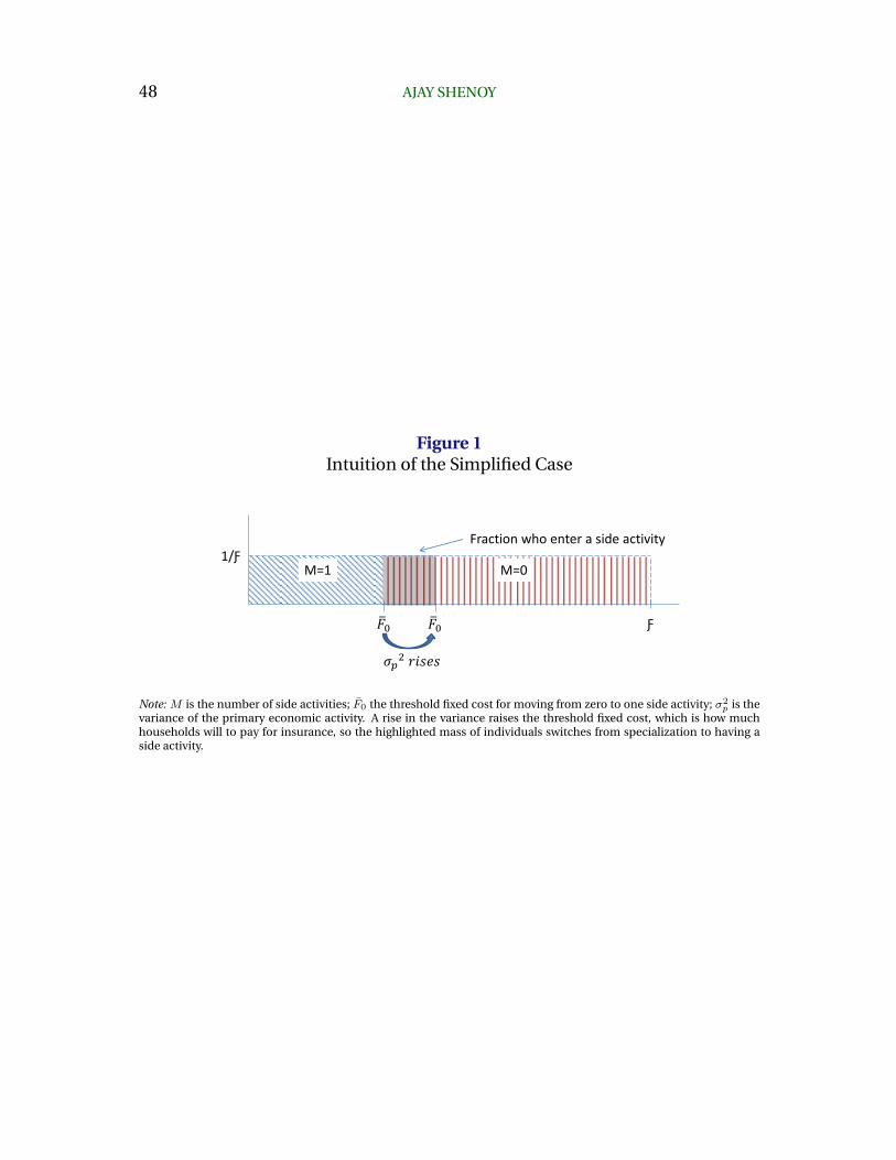
48 AJAY SHENOY

Figure 1Intuition of the Simplified Case

Ƒ

1/Ƒ M=0 M=1

𝜎𝑝2 𝑟𝑖𝑠𝑒𝑠

Fraction who enter a side activity

Suppose F has a uniform distribution over [0, Ƒ]

𝐹 0

A rise in the variance of the primary activity…

𝐹 0

…causes a rise in the maximal cost households are willing to pay…

…and causes the average number of activities to rise

Note: M is the number of side activities; F0 the threshold fixed cost for moving from zero to one side activity; σ2p is the

variance of the primary economic activity. A rise in the variance raises the threshold fixed cost, which is how muchhouseholds will to pay for insurance, so the highlighted mass of individuals switches from specialization to having aside activity.

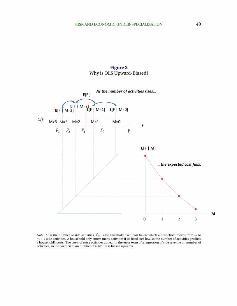
RISK AND ECONOMIC UNDER-SPECIALIZATION 49

Figure 2Why is OLS Upward-Biased?

Ƒ 𝐹 0

1/Ƒ M=0 M=1 M=2 M=3 M>3

E[F | M=0] E[F | M=1] E[F | M=2]

E[F | M=3]

E[F ]

F

E[F | M]

M 0 1 2 3

As the number of activities rises…

…the expected cost falls.

𝐹 1 𝐹 2 𝐹 3

Note: M is the number of side activities; Fm is the threshold fixed cost below which a household moves from m tom + 1 side activities. A household only enters many activities if its fixed cost low, so the number of activities predictsa household’s costs. The costs of extra activities appear in the error term of a regression of side revenue on number ofactivities, so the coefficient on number of activities is biased upwards.

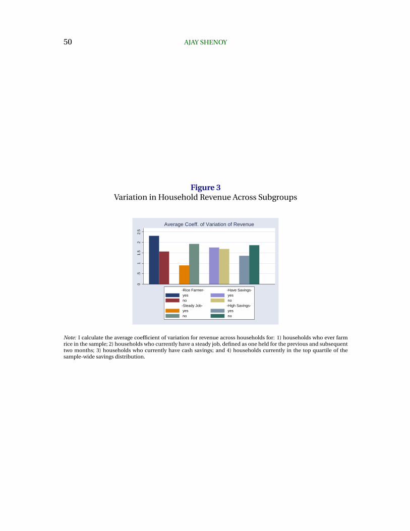
50 AJAY SHENOY

Figure 3Variation in Household Revenue Across Subgroups

0.5

11.

52

2.5

Average Coeff. of Variation of Revenue

-Rice Farmer- yes no-Steady Job- yes no

-Have Savings- yes no-High Savings- yes no

Note: I calculate the average coefficient of variation for revenue across households for: 1) households who ever farmrice in the sample; 2) households who currently have a steady job, defined as one held for the previous and subsequenttwo months; 3) households who currently have cash savings; and 4) households currently in the top quartile of thesample-wide savings distribution.

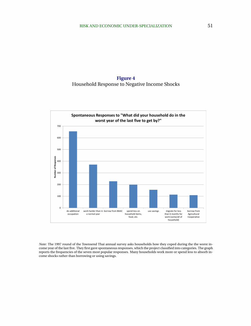
RISK AND ECONOMIC UNDER-SPECIALIZATION 51

Figure 4Household Response to Negative Income Shocks

0

100

200

300

400

500

600

700

do additionaloccupation

work harder than ina normal year

borrow from BAAC spend less onhousehold items,

food, etc.

use savings migrate for lessthan 6 months forwork (some/all of

household)

borrow fromAgriculturalCooperative

Num

ber o

f Respo

nses

Spontaneous Responses to "What did your household do in the worst year of the last five to get by?"

Note: The 1997 round of the Townsend Thai annual survey asks households how they coped during the the worst in-come year of the last five. They first gave spontaneous responses, which the project classified into categories. The graphreports the frequencies of the seven most popular responses. Many households work more or spend less to absorb in-come shocks rather than borrowing or using savings.

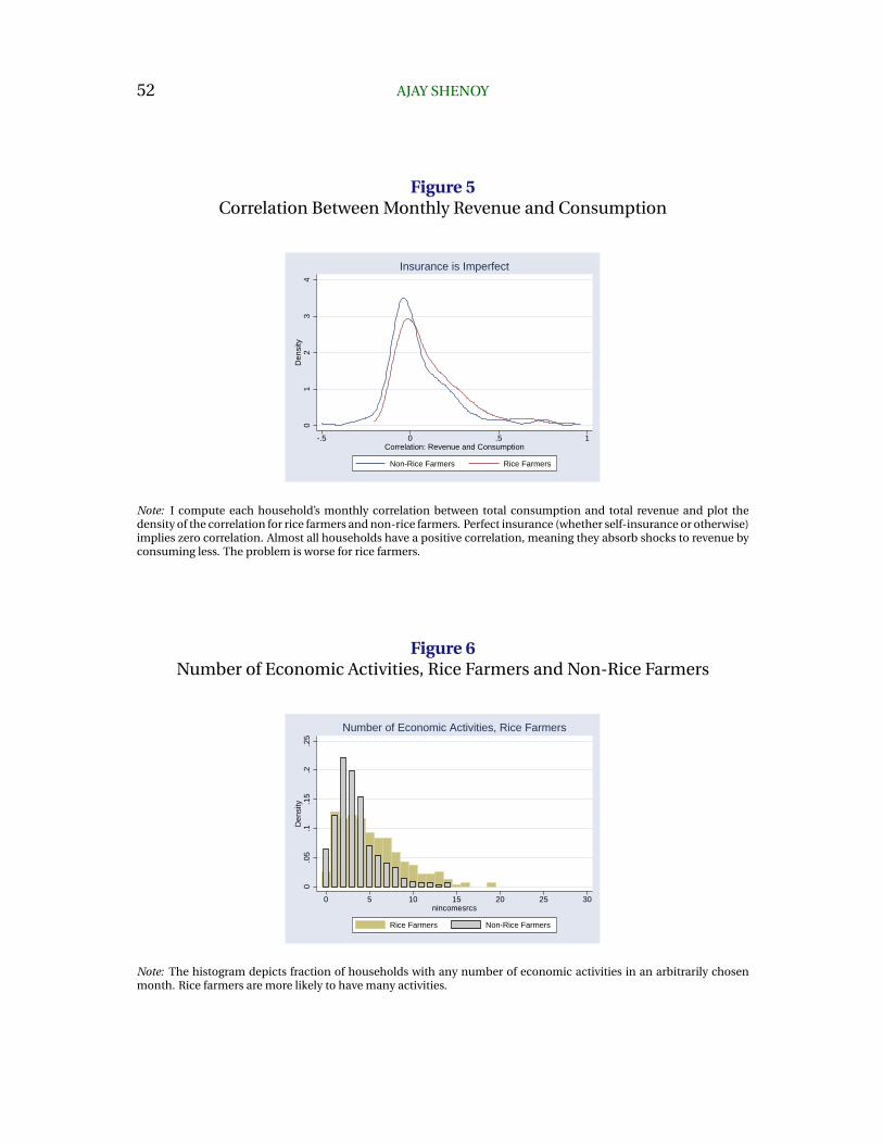
52 AJAY SHENOY

Figure 5Correlation Between Monthly Revenue and Consumption

01

23

4D

ensi

ty

-.5 0 .5 1Correlation: Revenue and Consumption

Non-Rice Farmers Rice Farmers

Insurance is Imperfect

Note: I compute each household’s monthly correlation between total consumption and total revenue and plot thedensity of the correlation for rice farmers and non-rice farmers. Perfect insurance (whether self-insurance or otherwise)implies zero correlation. Almost all households have a positive correlation, meaning they absorb shocks to revenue byconsuming less. The problem is worse for rice farmers.

Figure 6Number of Economic Activities, Rice Farmers and Non-Rice Farmers

0.0

5.1

.15

.2.2

5D

ensi

ty

0 5 10 15 20 25 30nincomesrcs

Rice Farmers Non-Rice Farmers

Number of Economic Activities, Rice Farmers

Note: The histogram depicts fraction of households with any number of economic activities in an arbitrarily chosenmonth. Rice farmers are more likely to have many activities.

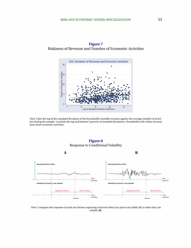
RISK AND ECONOMIC UNDER-SPECIALIZATION 53

Figure 7Riskiness of Revenue and Number of Economic Activities

05

1015

20N

umbe

r of

Eco

nom

ic A

ctiv

ities

7 8 9 10 11Log of Standard Deviation of Revenue

Std. Deviation of Revenue and Economic Activities

Note: I plot the log of the standard deviation of the household’s monthly revenue against the average number of activi-ties during the sample. I exclude the top and bottom 5 percent of standard deviations. Households with riskier revenuehave more economic activities.

Figure 8Response to Conditional Volatility

A B

Time (months)

Harvest

Expecting a harvest

Individual rice farmer’s crop calendar:

International Price of Rice:

Recent harvest

Time (months)

Time (months)

Harvest

Expecting a harvest

Individual rice farmer’s crop calendar:

International Price of Rice:

Recent harvest

Time (months)

Note: I compare the response of each rice farmer expecting a harvest when rice prices are stable (A) to when they arevolatile (B).

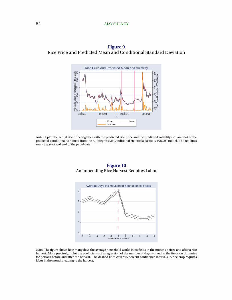
54 AJAY SHENOY

Figure 9Rice Price and Predicted Mean and Conditional Standard Deviation

Sample

1020

3040

5060

Std

. Dev

(H

undr

eds

of T

hai B

aht)

5010

015

020

025

030

0P

rice

and

Mea

n (H

undr

eds

of T

hai B

aht)

1980m1 1990m1 2000m1 2010m1t

Price MeanStd. Dev

Rice Price and Predicted Mean and Volatility

Note: I plot the actual rice price together with the predicted rice price and the predicted volatility (square root of thepredicted conditional variance) from the Autoregressive Conditional Heteroskedasticity (ARCH) model. The red linesmark the start and end of the panel data.

Figure 10An Impending Rice Harvest Requires Labor

010

2030

40

-5 -4 -3 -2 -1 0 1 2 3 4 5Months After a Harvest

Average Days the Household Spends on its Fields

Note: The figure shows how many days the average household works in its fields in the months before and after a riceharvest. More precisely, I plot the coefficients of a regression of the number of days worked in the fields on dummiesfor periods before and after the harvest. The dashed lines cover 95 percent confidence intervals. A rice crop requireslabor in the months leading to the harvest.

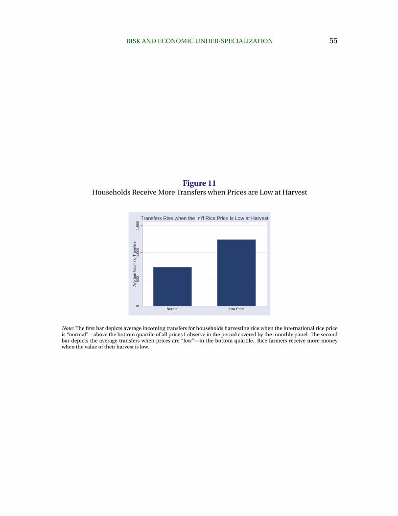
RISK AND ECONOMIC UNDER-SPECIALIZATION 55

Figure 11Households Receive More Transfers when Prices are Low at Harvest

050

01,

000

1,50

0A

vera

ge In

com

ing

Tra

nsfe

rs

Normal Low Price

Transfers Rise when the Int'l Rice Price Is Low at Harvest

Note: The first bar depicts average incoming transfers for households harvesting rice when the international rice priceis “normal”—above the bottom quartile of all prices I observe in the period covered by the monthly panel. The secondbar depicts the average transfers when prices are “low”—in the bottom quartile. Rice farmers receive more moneywhen the value of their harvest is low.

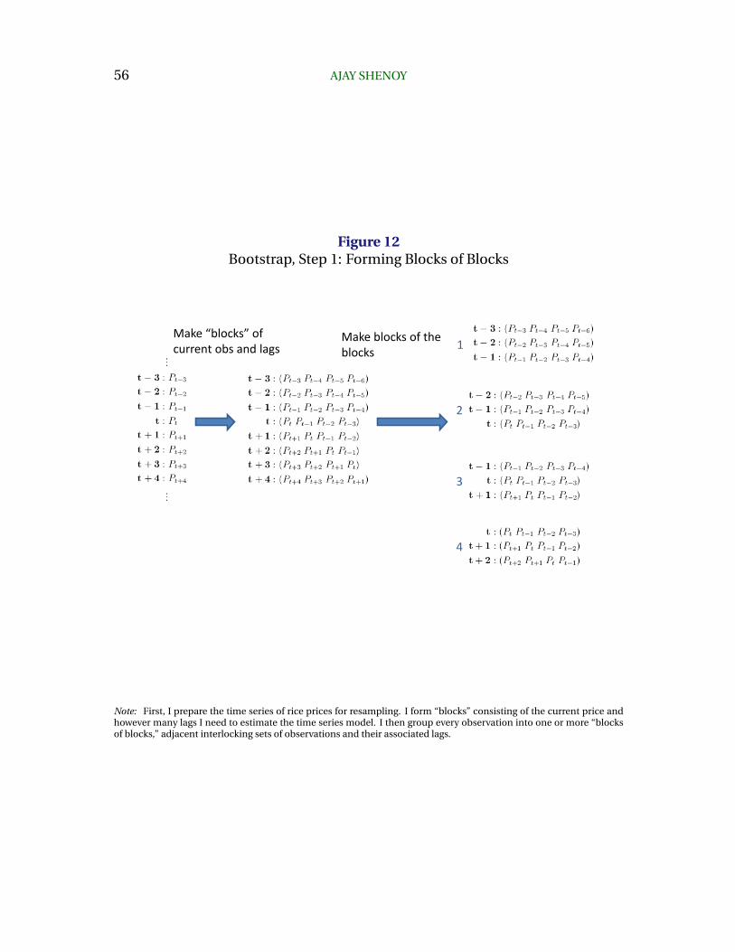
56 AJAY SHENOY

Figure 12Bootstrap, Step 1: Forming Blocks of Blocks

Make “blocks” of current obs and lags

Make blocks of the blocks

1

2

3

4

Note: First, I prepare the time series of rice prices for resampling. I form “blocks” consisting of the current price andhowever many lags I need to estimate the time series model. I then group every observation into one or more “blocksof blocks,” adjacent interlocking sets of observations and their associated lags.

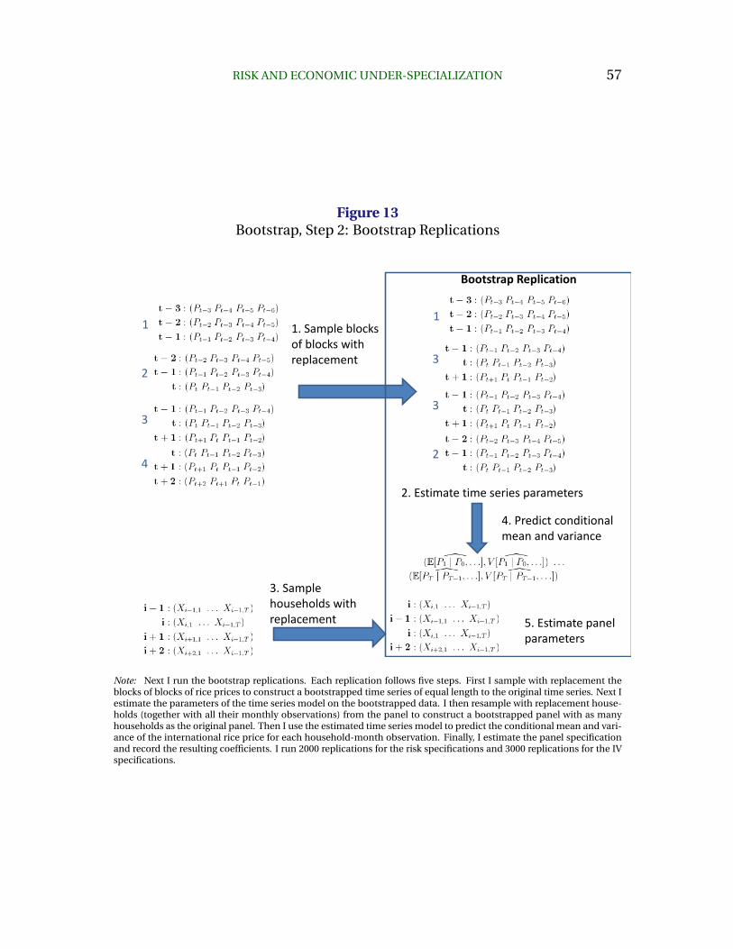
RISK AND ECONOMIC UNDER-SPECIALIZATION 57

Figure 13Bootstrap, Step 2: Bootstrap Replications

1

2

3

4

1. Sample blocks of blocks with replacement

1

3

3

2

2. Estimate time series parameters

3. Sample households with replacement

4. Predict conditional mean and variance

5. Estimate panel parameters

Bootstrap Replication

Note: Next I run the bootstrap replications. Each replication follows five steps. First I sample with replacement theblocks of blocks of rice prices to construct a bootstrapped time series of equal length to the original time series. Next Iestimate the parameters of the time series model on the bootstrapped data. I then resample with replacement house-holds (together with all their monthly observations) from the panel to construct a bootstrapped panel with as manyhouseholds as the original panel. Then I use the estimated time series model to predict the conditional mean and vari-ance of the international rice price for each household-month observation. Finally, I estimate the panel specificationand record the resulting coefficients. I run 2000 replications for the risk specifications and 3000 replications for the IVspecifications.

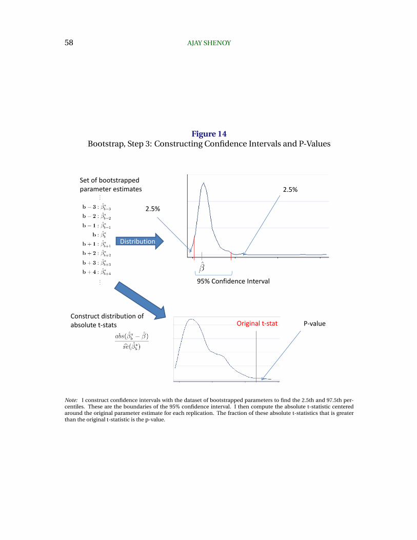
58 AJAY SHENOY

Figure 14Bootstrap, Step 3: Constructing Confidence Intervals and P-Values

Set of bootstrapped parameter estimates

2.5%

2.5%

95% Confidence Interval

Construct distribution of absolute t-stats Original t-stat P-value

Distribution

Note: I construct confidence intervals with the dataset of bootstrapped parameters to find the 2.5th and 97.5th per-centiles. These are the boundaries of the 95% confidence interval. I then compute the absolute t-statistic centeredaround the original parameter estimate for each replication. The fraction of these absolute t-statistics that is greaterthan the original t-statistic is the p-value.

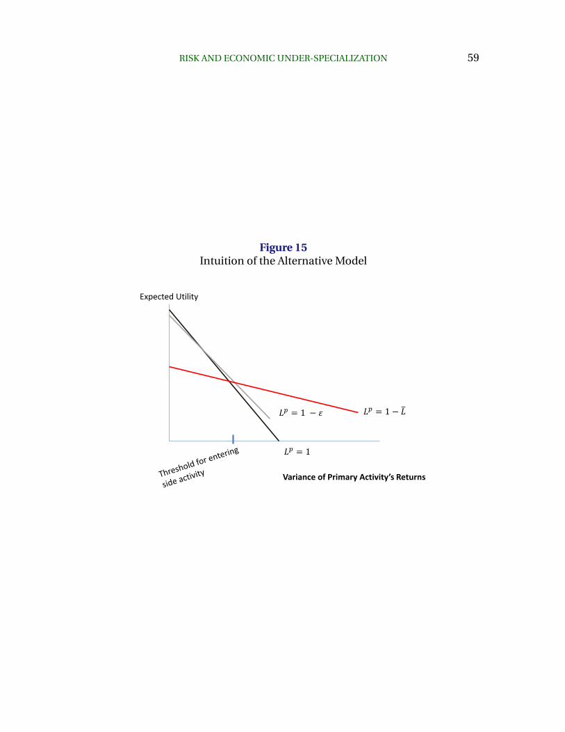
RISK AND ECONOMIC UNDER-SPECIALIZATION 59

Figure 15Intuition of the Alternative Model

Expected Utility

Variance of Primary Activity’s Returns

𝐿𝑝 = 1 − 𝜀 𝐿𝑝 = 1 − 𝐿

𝐿𝑝 = 1