Eur. Phys. J. E (2021) 44:129 https://doi.org/10.1140/epje/s10189-021-00131-9

THE EUROPEANPHYSICAL JOURNAL E

Regular Article – Soft Matter

Rigorous treatment of pairwise and many-bodyelectrostatic interactions among dielectric spheres at theDebye–Huckel levelO. I. Obolensky1,2, T. P. Doerr1, and Yi-Kuo Yu1,a

1 National Center for Biotechnology Information, National Library of Medicine, National Institutes of Health, Bethesda,MD 20894, USA

2 The A.F. Ioffe Institute, St. Petersburg, Russia

Received 5 August 2021 / Accepted 20 September 2021This is a U.S. government work and not under copyright protection in the U.S.; foreign copyrightprotection may apply 2021

Abstract Electrostatic interactions among colloidal particles are often described using the venerable (two-particle) Derjaguin–Landau–Verwey–Overbeek (DLVO) approximation and its various modifications. How-ever, until the recent development of a many-body theory exact at the Debye–Huckel level (Yu in Phys RevE 102:052404, 2020), it was difficult to assess the errors of such approximations and impossible to assessthe role of many-body effects. By applying the exact Debye–Huckel level theory, we quantify the errorsinherent to DLVO and the additional errors associated with replacing many-particle interactions by thesum of pairwise interactions (even when the latter are calculated exactly). In particular, we show that: (1)the DLVO approximation does not provide sufficient accuracy at shorter distances, especially when thereis an asymmetry in charges and/or sizes of interacting dielectric spheres; (2) the pairwise approximationleads to significant errors at shorter distances and at large and moderate Debye lengths and also gets worsewith increasing asymmetry in the size of the spheres or magnitude or placement of the charges. We alsodemonstrate that asymmetric dielectric screening, i.e., the enhanced repulsion between charged dielectricbodies immersed in media with high dielectric constant, is preserved in the presence of free ions in themedium.

1 Introduction

The search for methods providing more accurate descrip-tions and deeper understanding of electrostatic interac-tions among charged dielectric spheres in ionic solutionsremains, despite its long history, a subject of high inter-est, as proven by a persistent stream of theoretical andexperimental publications. This continued interest ismotivated by new types of dielectric objects that couldbe approximated by dielectric spheres and whose prop-erties and interactions are important for other fields ofphysics, chemistry, materials design and biology.

In order to describe charged dielectric spheres inionic solutions, it is desirable to choose models forthe charged dielectric spheres and the electrolyte solu-tion that may be productively combined, solved con-sistently, and, ideally, yield a rigorous solution. Themost straightforward formulation for the interaction ofthe charged dielectric spheres is a traditional differen-tial equation boundary value problem of electrostatics.Thus, one has to introduce a compatible model (differ-ential equation) for describing the ionic solution.

a e-mail: yyu@ncbi.nlm.nih.gov (corresponding author)

It is commonly accepted that, under not too extremecircumstances, each ion in the ionic solution can beconsidered freely diffusing through the solution in acanonically averaged electric potential φ(r), created byan “atmosphere” of other free ions and ionized col-loidal particles. On top of that, the ions are assumedto be thermalized according to Maxwell–Boltzmannstatistics. These assumptions give rise to the Poisson–Boltzmann equation:

∇2φ(r) = −4π

εo

∑

s

cs qs e−β qs φ(r), (1)

where qs and cs are the charge and average concentra-tion of the ions of species s, εo is the dielectric functionof the solution, and β is the inverse temperature. Itis worth mentioning that the solution of the Poisson–Boltzmann equation, while certainly being useful forproviding physical insights, cannot be held as a goldstandard of colloidal electrostatics. Indeed, as was orig-inally pointed out by Onsager [1] and Fowler [2], thesolutions of the Poisson–Boltzmann equation violate ageneral reciprocity principle, according to which thework done for bringing an ion j to its position rj inthe presence of ion k at position rk must be equal to

0123456789().: V,-vol 123

129 Page 2 of 18 Eur. Phys. J. E (2021) 44:129

the work done for bringing the ion k to position rk inthe presence of ion j at position rj [3–6] (see a briefdiscussion of this in Appendix A).

If the average potential φ(r) is sufficiently smallthroughout the solution, β qs φ(r) � 1, the exponen-tial in Eq. (1) can be expanded into a power series andonly the first-order term kept, as was originally done byDebye and Huckel [7] (the zeroth-order term vanishesdue to the overall charge neutrality):

∇2φ(r) = κ2φ(r), (2)

where

κ =

√4π

β

εo

∑

s

csq2s (3)

is the inverse Debye screening length. Using the Debye–Huckel equation (2) instead of the Poisson–Boltzmannequation (1) may in fact be more justified physicallyas, in the words of Lars Onsager, “... as soon asthe higher terms in the Poisson–Boltzmann equationbecome important, we can no longer expect the ionicatmospheres to be additive, and then the Poisson–Boltzmann equation itself becomes unreliable.” [3]

Importantly, not only does the solution of the Debye–Huckel equation satisfy the reciprocity principle, it canfurther be shown [5] that it is the exact small κ lim-iting form of the Poisson equation for the canonicallyaveraged potential. Thus, curiously, the Debye–Huckelequation has in some ways a firmer physical foundationthan the Poisson–Boltzmann equation, in spite of thefact that the former is obtained as a linearization of thelatter. Moreover, the range of validity and utility of theDebye–Huckel equation may be expanded by choosingκ appropriately [8–11]. Since the Debye–Huckel equa-tion obeys certain symmetries violated by the Poisson–Boltzmann equation, allows for rigorous solution, andcan have its range of applicability extended by consid-ering κ to be an effective parameter, the Debye–Huckeltheory seems a desirable choice for combining with atheory of charged dielectric spheres. There are fieldtheoretical [12] and integral equation [13] techniquesfor investigating the thermodynamics of ionic solutionsthat can potentially address the nonlinear regime. How-ever, as we are attempting to combine an electrolytetheory with an electrostatic boundary value problem,and we further anticipate application for simulations,such methods do not seem appropriate for the purposesconsidered here.

However, one needs to be careful to verify that theDebye–Huckel linearization is valid. In order to do so,one needs to actually solve the electrostatics prob-lem and find the maximum magnitude of the poten-tial, making sure that it is smaller than 1/β = kBT(≈ 26 meV for a solution at 298 K).

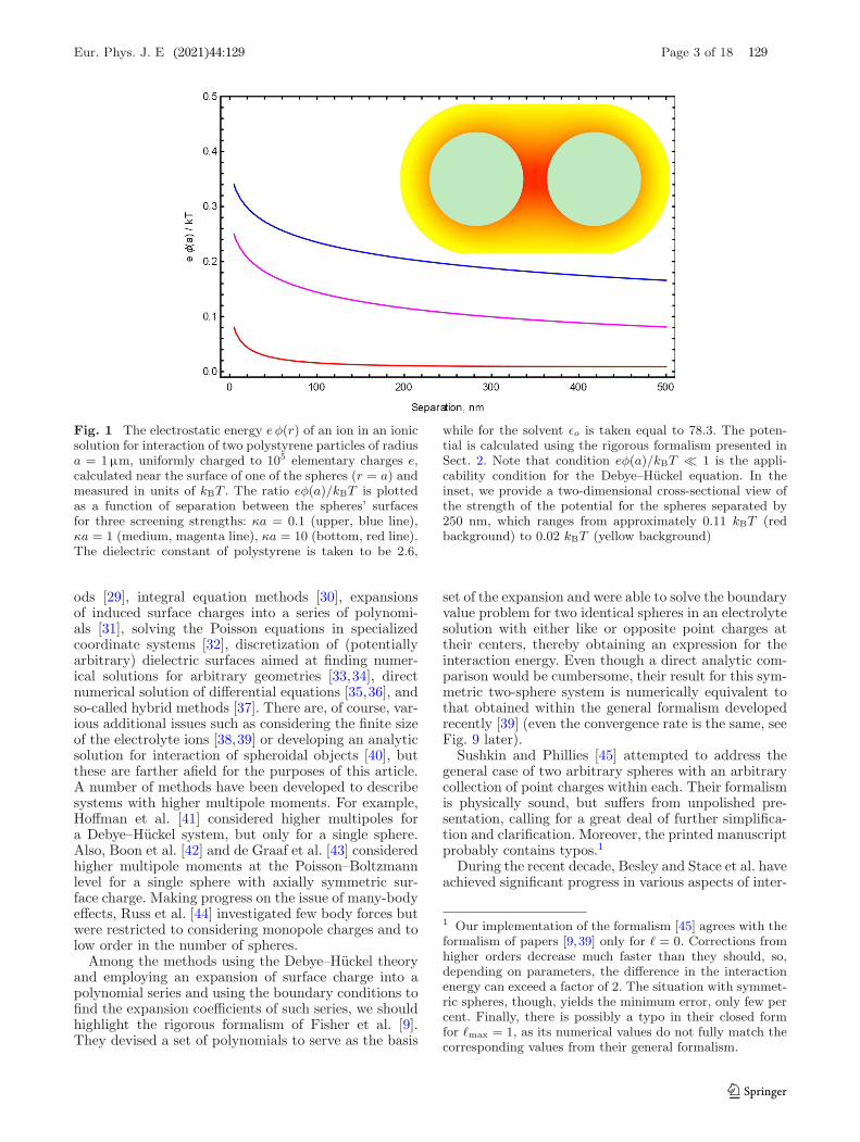
In Fig. 1, we plot the electrostatic energy e φ(r) of anion in an ionic “atmosphere”, in the units of kBT , asa function of the distance between the surfaces of two

spheres. The potential is obtained as the rigorous solu-tion at the Debye–Huckel level (see Sect. 2) and is calcu-lated at a point where it attains its maximum value, atthe surface of one of the spheres, and at the point closestto the other sphere. The parameters of this two-spheresystem were chosen to be similar to conditions used ina set of optical tweezer experiments that measured theinteraction force between two charged colloidal parti-cles [14]. We see from the figure that for polystyreneparticles of radius a = 1µm, uniformly charged to 105elementary charges e, the Debye–Huckel linearization isvalid up to the point where the spheres touch.

The Debye–Huckel linearization is generally lessaccurate for weaker solutions (smaller screening strengthκa), as it is clearly seen in Fig. 1. For demonstrationpurposes, the smallest κa we used in Fig. 1 was 0.1,while the molarities used in the experiment [14] wouldresult in κa ranging in tens and hundreds. Therefore,the Debye–Huckel equation would still be applicableeven if the colloidal particles were even more highlycharged.

Another important conclusion that can be drawnfrom Fig. 1 is that calculating potential at the surfaceof an isolated sphere in an ionic solution may not besufficient for judging the validity of the Debye–Huckellinearization. Indeed, the potential is greatly enhancedwhen two spheres interact with each other. The poten-tial can increase several fold when two charged spheresare in a close proximity, due to significant values ofinduced surface charge. This circumstance makes find-ing an accurate solution to the electrostatic problemeven more crucial.

Soon after Debye and Huckel proposed their lin-earized Poisson–Boltzmann model for describing prop-erties of electrolytes [7], the question of how to correctlydescribe within this model the interaction betweencharged dielectric bodies was actively debated [15–19].It was unclear what role the van der Waals interactionplays as compared to the direct electrostatic interactionand even whether electrostatic interaction between sim-ilarly charged particles is repulsive or attractive due tothe presence of free ions in the solution [20,21].

The consensus model was formulated by Derjaguinand Landau [22,23] and independently by Verwey andOverbeek [24], colloquially joined together and knownas the DLVO theory [25]. The DLVO approximation(with or without the ad hoc van der Waals term) iswidely used when a quick estimate of interaction energyor force is needed [26]. While the DLVO energy is beau-tiful in its simplicity and physical clarity and remains inuse (see, for a recent example, Ref. [27]), its numericalaccuracy and the range of phenomena it can captureare inherently limited.

Beyond the DLVO approximation, there exists a verywide variety of theoretical approaches to colloidal par-ticles in an ionic solution. Not aiming at giving a com-prehensive review of these efforts and focusing primar-ily (but not exclusively) on studies considering dielec-tric spheres in electrolyte solutions, we can refer thereader to some recent works in the field, employingthe method of image charges [28], perturbative meth-

123

Eur. Phys. J. E (2021) 44:129 Page 3 of 18 129

Fig. 1 The electrostatic energy e φ(r) of an ion in an ionicsolution for interaction of two polystyrene particles of radiusa = 1µm, uniformly charged to 105 elementary charges e,calculated near the surface of one of the spheres (r = a) andmeasured in units of kBT . The ratio eφ(a)/kBT is plottedas a function of separation between the spheres’ surfacesfor three screening strengths: κa = 0.1 (upper, blue line),κa = 1 (medium, magenta line), κa = 10 (bottom, red line).The dielectric constant of polystyrene is taken to be 2.6,

while for the solvent εo is taken equal to 78.3. The poten-tial is calculated using the rigorous formalism presented inSect. 2. Note that condition eφ(a)/kBT � 1 is the appli-cability condition for the Debye–Huckel equation. In theinset, we provide a two-dimensional cross-sectional view ofthe strength of the potential for the spheres separated by250 nm, which ranges from approximately 0.11 kBT (redbackground) to 0.02 kBT (yellow background)

ods [29], integral equation methods [30], expansionsof induced surface charges into a series of polynomi-als [31], solving the Poisson equations in specializedcoordinate systems [32], discretization of (potentiallyarbitrary) dielectric surfaces aimed at finding numer-ical solutions for arbitrary geometries [33,34], directnumerical solution of differential equations [35,36], andso-called hybrid methods [37]. There are, of course, var-ious additional issues such as considering the finite sizeof the electrolyte ions [38,39] or developing an analyticsolution for interaction of spheroidal objects [40], butthese are farther afield for the purposes of this article.A number of methods have been developed to describesystems with higher multipole moments. For example,Hoffman et al. [41] considered higher multipoles fora Debye–Huckel system, but only for a single sphere.Also, Boon et al. [42] and de Graaf et al. [43] consideredhigher multipole moments at the Poisson–Boltzmannlevel for a single sphere with axially symmetric sur-face charge. Making progress on the issue of many-bodyeffects, Russ et al. [44] investigated few body forces butwere restricted to considering monopole charges and tolow order in the number of spheres.

Among the methods using the Debye–Huckel theoryand employing an expansion of surface charge into apolynomial series and using the boundary conditions tofind the expansion coefficients of such series, we shouldhighlight the rigorous formalism of Fisher et al. [9].They devised a set of polynomials to serve as the basis

set of the expansion and were able to solve the boundaryvalue problem for two identical spheres in an electrolytesolution with either like or opposite point charges attheir centers, thereby obtaining an expression for theinteraction energy. Even though a direct analytic com-parison would be cumbersome, their result for this sym-metric two-sphere system is numerically equivalent tothat obtained within the general formalism developedrecently [39] (even the convergence rate is the same, seeFig. 9 later).

Sushkin and Phillies [45] attempted to address thegeneral case of two arbitrary spheres with an arbitrarycollection of point charges within each. Their formalismis physically sound, but suffers from unpolished pre-sentation, calling for a great deal of further simplifica-tion and clarification. Moreover, the printed manuscriptprobably contains typos.1

During the recent decade, Besley and Stace et al. haveachieved significant progress in various aspects of inter-

1 Our implementation of the formalism [45] agrees with theformalism of papers [9,39] only for � = 0. Corrections fromhigher orders decrease much faster than they should, so,depending on parameters, the difference in the interactionenergy can exceed a factor of 2. The situation with symmet-ric spheres, though, yields the minimum error, only few percent. Finally, there is possibly a typo in their closed formfor �max = 1, as its numerical values do not fully match thecorresponding values from their general formalism.

123

129 Page 4 of 18 Eur. Phys. J. E (2021) 44:129

actions between two dielectric bodies in vacuum and inan electrolyte medium, reported in a series of papers[40,46–51]. Their formalism [46], although imposingazimuthal symmetry with respect to the axis connect-ing the centers of the two spheres, was demonstrated toprovide useful insights, such as dependence of attrac-tion between two spheres with same charge immersedin a medium of lower dielectric constant on asymmetryof charge and radii of the interacting spheres [47,50].Their analysis uses a re-expansion of modified Besselfunctions about a new center to allow matching ofthe boundary conditions at the surface of each sphere.However, multiple re-expansions are required in orderto obtain the necessary Legendre polynomials, makingcontrolling the numerical accuracy somewhat difficultsince rather than a single maximum multipole �max, themultiple re-expansions introduce additional sums thatneed to be cut off in a consistent manner.

In a series of efforts [52–55], we have undertaken thedevelopment of a rigorous method for determining toany desirable precision the interaction energies for anarbitrary number of dielectric spheres in a dielectricmedium. The most recent work [39] contains a generalformalism, rigorous within the Debye–Huckel approx-imation, for describing interactions among dielectricspheres immersed in an electrolyte solution. The onlyother surface charge method of a similar generalityand rigor that we are aware of is due to Lotan andHead-Gordon [56]. The downside of their method, how-ever, is that transformations of coordinates when re-expanding at different locations are handled via an iter-ative numerical procedure. This significantly compli-cates computations, reduces their efficiency, and, evenmore importantly, introduces another source of uncer-tainty in the accuracy of the numerical results on top ofcutting off polynomial expansions of the surface chargedistributions.

In this article, we apply the general formalism [39]to detailed analysis of interactions in the case of two,three and four spheres. A terse summary of the generalformalism may be found in Appendix B. We work outthe simplifications that are possible for the particularcase of two spheres and even further simplifications forthe case of two spheres with axially symmetric chargedistributions. In the latter case, it is possible to derivea simple expression for the force in terms of the sameset of linear equations as for the energy. The significantnew physical results are as follows. We demonstrate inSect. 2.1 that asymmetric dielectric screening [52,57],i.e., the enhanced repulsion between charged dielectricbodies immersed in media with high dielectric constant,known to occur in the absence of ions, is preserved inthe presence of free ions in the medium. In Sect. 3, wecompare the baseline DLVO approximation [25] to theresults of the rigorous formalism. Indeed, only by com-paring to the exact solution of the Debye–Huckel prob-lem can the accuracy of DLVO theory (or any of itsproposed modifications or replacements) be correctlyand reliably assessed. We highlight the circumstancesunder which one can expect larger errors for the DLVOtheory. In the last section, we discuss the accuracy of

approximating the full interaction energy as a sum ofpairwise interactions using examples of three- and four-sphere systems. Finally, we illustrate how the speed ofconvergence depends on variation of radii, charge mag-nitude and charge placement in the system.

2 Two spheres

In order to represent charged colloidal particles inan ionic solution, we consider a system of dielectricspheres in a medium (water) with dielectric constantεo containing freely diffusing, thermalized ions. Spherei has dielectric constant εi, radius ai, position ri,and free charge that can be represented by standardelectric multipole moments qlm (l = 0, 1, . . . ,∞ andm = −l, −l+1, . . . , l) or equivalently [39,54] by surfacemoments Qlm. This free charge distribution is fixed (wedo not consider a dynamic chemical charge regulationscheme for the free charge), but there will be additionalinduced charge at the interface between the regions ofdiffering dielectric constant. The spheres are embeddedin an electrolyte solution that will be modeled by theDebye–Huckel theory and whose properties are there-fore summarized by the inverse Debye screening lengthκ. We will, for the most part, regard κ as a parameter.Thus, Eq. (3) will not be binding.

Within the framework of the general formalism forthis system developed in Ref. [39] and briefly recapitu-lated in Appendix B, the distribution of the fixed (alsocalled free) charge ρ(s) at each sphere is expanded intoa series using the basis set of spherical harmonics Y�m.The (yet unknown) induced charge distribution at eachsphere is also expanded with the same basis set, andthe boundary conditions on the potential at the surfaceof each sphere then lead to a system of linear equa-tions. The variables in this system are scaled sphericalcomponents of the net (free + induced) charge distri-bution Q+

�m. Having determined these components bysolving the system of equations, one can subsequentlyfind the induced charge distributions on each sphere,the electric potential at any point of space, as well asthe electrostatic interaction energy.

2.1 Two spheres with arbitrary charge distributions

For a system of only two spheres, the general system oflinear equations simplifies not only due to fewer expan-sion centers, but also due to the fact that for two spheresthere is only one vector connecting the centers of thespheres, and this vector L ≡ L1→2 = −L2→1 can alwaysbe directed along the z-axis. The spherical harmonicsdepending on the orientation of this vector are, there-fore, only nonzero for zero momentum projections:

Y�2m2

(L1→2

)=

√2�2 + 1

4πδm20,

Y�2m2

(L2→1

)= (−1)�2

√2�2 + 1

4πδm20. (4)

123

Eur. Phys. J. E (2021) 44:129 Page 5 of 18 129

As small as it seems, this circumstance allows oneto derive a quite simple, yet still rigorous, system ofequations for solving the electrostatics problem of twospheres in an ionic solution.

With (4) in mind, the general system of equations(39) can be reduced to:

Q1�m = i� (κa1) k� (κa1) K (�, κa1) Q1+

�m

+∑

�1

(−1)�1 i�(κa1) i�1 (κa2) I (�, κa1) H�m�1(κL) Q2+�1m

Q2�m = i� (κa2) k� (κa2) K (�, κa2) Q2+

�m

+∑

�1

(−1)� i� (κa2) i�1 (κa1) I (�, κa2) H�m�1(κL)Q1+�1m.

(5)

Here for convenience we use explicit enumeration ofthe spheres. The source terms in (5) are the spheri-cal components of the free charge distribution (surfacemoments) Q�m,

Q�m ≡√

4πq �m

a�=

√4π

a�

∫ρ(s ) s� Y ∗

�m(s) ds , (6)

where a is the sphere’s radius and q �m are regular mul-tipole moments of the charge distribution ρ(s).

As is expected for a spherical harmonics expansionfor a Helmholtz equation, the radial coefficients arethe modified spherical Bessel functions: i�(z) are themodified spherical Bessel functions of the first kindwith i�(z) = (i)−�j�(i z), while k�(z) are the modi-fied spherical Bessel functions of the second kind withk�(z) = −(i)�h

(1)� (i z). The functions are calculated at

the dimensionless radius of one of the spheres κa1 orκa2.

The functions K(�, x) and I(�, x) are introducedsolely for the brevity of notation; they depend on thedielectric constant of the medium εo and on the dielec-tric constant ε of the corresponding sphere:

K(�, x) = x

[� (ε − εo) +

x k�+1(x)k�(x)

εo

],

I(�, x) = x

[� (ε − εo) − x i�+1(x)

i�(x)εo

]. (7)

Finally, the function H�m�1(κL) is defined as:

H�m�1(κL) = (−1)m√

(2� + 1) (2�1 + 1)�+�1∑

�2=|�−�1|C�2 0

� 0 �10C�2 0

� m �1 −m k�2(κL),

(8)

it is a reduced version of a more general factorH�m�1m1(κLk→j), Eq. (36), that in the general formal-ism takes care of the mutual location and orientation ofdifferent spheres. Note, the quantity H�m�1(κL) is sym-metric with respect to the interchange � ↔ �1, allowing

for a more efficient numerical implementation and fur-ther simplifications.

With the above definitions, the system of linear equa-tions (5) with an appropriately chosen maximum num-ber of components �max can be solved, and the unknowncomponents of the scaled net charge distributions Q1+

�m

and Q2+�m can thus be determined.

Now, with the known Q1+�m and Q2+

�m, the interactionenergy can be found as:

Uint =κ

2

∑

�m

[i� (κa1) k� (κa1) Q

1∗�m Q1+

�m − Q1∗�m Q

1

�m

K (�, κa1)

]

+κ

2

∑

�m

[i� (κa2) k� (κa2) Q

2∗�m Q2+

�m − Q2∗�m Q

2

�m

K(�, κa2)

]

+κ

2

∑

�m

∑

�1

(−1)�1 H�m�1(κL) il (κa1) i�1 (κa2)

[Q

1∗�m Q2+

�1m + Q1+�m Q

2∗�1m

]. (9)

Note that Eqs. (5) and (9) present a general, rigorous atthe Debye–Huckel level, formalism for determining theinduced charges and interaction energies for the case oftwo dielectric spheres in an ionic solution. There are norestrictions on the free charge distributions Q

1

�m andQ

2

�m.The components of the net charge distributions Q1+

�m

and Q2+�m can also be used to determine the electrostatic

potential between the spheres as:

Φ (r1) =√

4π κ∑

�m

[k�(κr1)Y�m(r1) i�(κa1) Q1+

�m

+ i� (κr1) Y�m (r1)∑

�1

(−1)�1 i�1 (κa2)

H�m�1(κL) Q2+�1m

]. (10)

Here r1 is the point where the potential is to be found.We chose the system of coordinates to be associatedwith the first sphere, but the second sphere’s coordi-nates can also be used with the appropriate change ofindices. The direction of the vector r1 can be arbitrary,but the distance where Eq. (10) is valid is limited bythe inequality a1 < r1 < L − a2.

As an illustration of capabilities of this generalmethod, let us consider electrostatic interaction ina non-axially symmetric system. In Fig. 2, we plotinteraction energies between two spheres with physi-cal dipoles oriented perpendicular to L1→2. The dipolesare created by two point charges, shifted from the cor-responding sphere’s center by half of its radius. Thecharges are equal in magnitude and opposite in sign, sothe net charge of each sphere is zero. The interactionenergy is calculated for three different orientations ofthese dipoles: parallel, anti-parallel and orthogonal. Asexpected, the spheres with parallel dipoles repel andthe spheres with anti-parallel dipoles attract.

123

129 Page 6 of 18 Eur. Phys. J. E (2021) 44:129

Fig. 2 The interaction energies in atomic units betweentwo spheres with off-center point charges. Each sphere hastwo equal in magnitude and opposite in sign point charges(the net charge is zero), shifted from the center in oppositedirections by half of the radius. The dipoles are orthogo-nal to the line connecting the centers of the spheres. Theinteraction energy is calculated for three different orien-

tations of these dipoles: parallel (red), anti-parallel (blue)and perpendicular (magenta). Half the sum of red and bluecurves (the asymmetry of repulsion and attraction) alsoyield the magenta line exactly. The dimensionless screeningstrength is κa = 0.1. The radii and point charges are one inatomic units, the dielectric constants inside the spheres areε1 = ε2 = 4, and εo = 80 for the medium

There are two noteworthy features, however, inFig. 2. The first one is the asymmetry in repulsionof parallel dipoles and attraction of anti-parallel ones.This stems from asymmetric dielectric screening [52],a known effect in the interaction between dielectricobjects whereby either repulsion (if εin < εout) orattraction (if εin > εout) is enhanced as compared tointeraction of point charges. For a discussion and anapplication of this effect to interaction of dielectricspheres, see, e.g., Refs. [50,57]. The second notewor-thy feature is the fact that the interaction between twoorthogonal dipoles (shown in magenta) is not zero, asone might have anticipated. Indeed, if the dielectricspheres were absent, then the interaction would vanish.However, the asymmetric dielectric screening is an inde-pendent feature due to the dielectric mismatch betweenthe spheres and the solvent and persists even when theinteractions of the point charges cancel.

2.2 Two spheres with axially symmetric chargedistributions

When axial symmetry is lacking, such as in the exampleof two dipoles considered above, all the components of

the scaled free and net charge distributions, Q�m andQ+

�m, can be nonzero. This means that one has to solvethe complete system of 2(�max + 1)2 linear equations(5). However, in the case of axial symmetry, only them = 0 components Q�0 and Q+

�0 will be nonzero. Thenew system will only have 2(�max + 1) equations, andthe calculations will simplify drastically.

System (5) is then reduced to:

Q1�0 = i� (κa1) k� (κa1) K (�, κa1) Q1+

� 0

+∑

�1

(−1)�1 i� (κa1) i�1 (κa2) I (�, κa1) H� 0 �1(κL) Q2+�10

Q2�0 = i� (κa2) k� (κa2) K (�, κa2) Q2+

� 0

+∑

�1

(−1)� i� (κa2) i�1 (κa1) I (�, κa2) H� 0 �1(κL) Q1+�10

.

(11)

For further simplification, one can use explicit expres-sions for Clebsch–Gordan coefficients with zero momen-tum projections [58] to obtain H� 0 �1(κL) in terms offactorials,

H� 0 �1(κL)=√

(2� + 1)(2�1 + 1)

×�+�1∑

�2=|�−�1|

(√2�2 + 1 g!

√(2g − 2�)! (2g − 2�1)! (2g − 2�2)!

(g − �)! (g − �1)! (g − �2)!√

(2g + 1)!

)2

k�2(κL), (12)

123

Eur. Phys. J. E (2021) 44:129 Page 7 of 18 129

where 2g = � + �1 + �2 must be even.Moreover, it is now easy to find the force acting on

each sphere, because for charge distributions axiallysymmetric around the vector L, the force is directedalong L. In this case, in order to determine the force,we can take a derivative of the interaction energy withrespect to the distance L (instead of taking a gradientas in the most general case):

F =−∂Uint

∂L=

κ2

2

∑

�

[i�(κa1) k�(κa1) Q

1∗�0

(− ∂Q1+

�0

∂(κL)

)

+i�(κa2) k� (κa2) Q2∗�0

(− ∂Q2+

�0

∂(κL)

)]

+κ2

2

∑

�

∑

�1

(−1)�1

(−dH� 0 �1(κL)

d(κL)

)

il(κa1) i�1(κa2)[Q

1∗�0 Q2+

�10+ Q1+

�0 Q2∗�10

]

+κ2

2

∑

�

∑

�1

(−1)�1 H� 0 �1(κL) il(κa1) i�1(κa2)

×[Q

1∗�0

(− ∂Q2+

�10

∂(κL)

)+

(− ∂Q1+

�0

∂(κL)

)Q

2∗�10

].

(13)

For computational purposes, one can again expressthe derivative of the modified spherical Bessel as inEq. (41):

∂k�(x)∂x

=� k�(x) − x k�+1(x)

x. (14)

The derivatives of the components of the scaled netcharge distributions Q+

� 0 can be found by taking deriva-tives of both parts of Eq. (11):

0 = i�(κa1) k�(κa1)K(�, κa1)

(∂Q1+

� 0

∂(κL)

)

+∑

�1

(−1)�1 i�(κa1) i�1(κa2) I (�, κa1)

[dH� 0 �1(κL)

d(κL)Q2+

�1 0 + H� 0 �1(κL)

(∂Q2+

�10

∂(κL)

)]

0 = i�(κa2) k�(κa2)K(�, κa2)

(∂Q2+

� 0

∂(κL)

)

+∑

�1

(−1)� i�(κa2) i�1(κa1) I (�, κa2)

[dH� 0 �1(κL)

d(κL)Q1+

�1 0 + H� 0 �1(κL)

(∂Q1+

�1 0

∂(κL)

)]

(15)

Assuming that the system of linear equations (11) hasalready been solved and introducing quantities

Θ1� ≡ (−1)� i� (κa2) I (�, κa2)

∑

�1

i�1 (κa1) H′� 0 �1(κL) Q1+

�10

Θ2� ≡ i� (κa1) I (�, κa1)

∑

�1

(−1)�1 i�1 (κa2) H′� 0 �1(κL) Q2+

�10,

(16)

we obtain a system of linear equations for the negativederivatives:

Θ2� = i� (κa1) k� (κa1) K (�, κa1)

(− ∂Q1+

� 0

∂(κL)

)

+∑

�1

(−1)�1 i� (κa1) i�1 (κa2) I (�, κa1) H� 0 �1(κL)

(−∂Q2+

�10

∂(κL)

)

Θ1� = i� (κa2) k� (κa2) K (�, κa2)

(− ∂Q2+

� 0

∂(κL)

)

+∑

�1

(−1)� i� (κa2) i�1(κa1) I (�, κa2) H� 0 �1(κL)

(−∂Q1+

�10

∂(κL)

)(17)

Note that systems (11) and (17) have the same matrixof coefficients; only the source terms are different. Thismakes a computational implementation of force calcu-lation much more efficient.

This increased computational efficiency, appearingin the case of axially symmetric systems due to thereduced size of matrix (11) and the possibility of itsre-purposing for determining the force, allows calculat-ing electrostatic interactions in a rigorous fashion downto very short distances, almost to the touching point,where the number of contributing terms may increaseto hundreds.

Janus particles (see, e.g., a recent paper [59]) couldserve as a practical example of such an axially sym-metric system. Within the present formalism, they areeasily modeled as two patches of positive and negativecharge, uniformly distributed over a spherical cap of apolar angle θ0. In this case, the spherical componentsof the free charge are given by:

Q00 = 0

Q�m =[1 − (−1)�

] q√2� + 1

P�−1 (cos θ0) − P�+1 (cos θ0)1 − cos θ0

δm 0, � > 0,

(18)

where P�(x) are Legendre polynomials. It is interestingto note that for reasonable values of the opening polar

123

129 Page 8 of 18 Eur. Phys. J. E (2021) 44:129

angle θ0 the scaled free charge components are close tothose of a simple dipole oriented along the z-axis, ascan be seen from the small-θ0 expansion

Q�m =[1 − (−1)�

] √2� + 1 q

[1− �(� + 1)

4(1−cos θ0)

]δm 0.

(19)Our numerical results confirm this conclusion.

Another instance of a directly observable situationwhere an axially symmetric charge distribution mightprove useful is modeling interaction of two dielectricbeads that are attached to a support. For example, in anoptical tweezers experiment one of the colloid particlesis held in place by a pipette [14], which makes an oth-erwise spherically uniform charge distribution only axi-ally symmetric. (Our calculations show that the pres-ence of a pipette in these kinds of experiment would beimportant for low κa regimes.)

2.3 Two spheres with point charges at their centers

Finally, let us write down the expressions for the inter-action energy and the force for the important case whenboth spheres have only one point charge located attheir center. Let’s denote these charges q1 and q2. Then,according to Eq. (6),

Qk

� m = qk δ� 0 δm0. (20)

The interaction energy now has two simple terms cen-tered at each sphere and only one summation in thecross term. Indeed, only the � = 0, m = 0 componentsin the first two sums in Eq. (9) survive, while the com-pounded sum over �, m and �1 in the third term turnsinto two independent sums over � and �1 (which can becombined by renaming �1 back to �).

Using the explicit expressions for zero-order modi-fied spherical Bessel functions, k0(κa) = e−κa/(κa),i0(κa) = sinh(κa)/(κa), and noting that H� 0 0(κL) =√

(2� + 1) k�(κL), we obtain

Uint (q1; q2) =q1

2a1

[sinh (κa1)

κa1e−κa1 Q

1+00 − 1

εo

q1

1 + κa1

]

+q2

2a2

[sinh (κa2)

κa2e−κa2 Q

2+00 − 1

εo

q2

1 + κa2

]

+1

2

∑�

√(2�+1)k�(κL)

[i� (κa1) sinh (κa2)

q2

a2Q

1+� 0

+(−1)�i�(κa2) sinh(κa1)

q1

a1Q

2+� 0

]. (21)

Consequently, the force is

F = −∂Uint

∂L=

q1

2a21

sinh(κa1) e−κa1

(− ∂Q1+

00

∂(κL)

)

+q2

2a22

sinh(κa2) e−κa2

(− ∂Q2+

00

∂(κL)

)

+κ

2

∑

�

√(2� + 1) k′

�(κL)

[i�(κa1) sinh(κa2)

q2

a2Q1+

� 0

+(−1)� i�(κa2) sinh(κa1)q1

a1Q2+

� 0

]

+κ

2

∑

�

√(2� + 1) k�(κL)

[i�(κa1) sinh(κa2)

q2

a2

(− ∂Q1+

� 0

∂(κL)

)

+(−1)� i�(κa2) sinh(κa1)q1

a1

(− ∂Q2+

� 0

∂(κL)

)], (22)

where the components of the scaled net charge distribu-tions Q+

� 0 are found by solving the system of equations

(11) with Qk

� 0 = qk δ� 0. Their derivatives are found bysolving system (17).

3 Comparison with the DLVO theory

The presented formalism is exact and therefore allowsa quantitative characterization of errors arising fromusing the DLVO approximation. Within the DLVOapproximation, the electrostatic interaction energy isgiven by the term:

UDLVOint =

q1 q2εoL

e−κD

(1 + κa1)(1 + κa2), (23)

where D = L − a1 − a2 is the separation between thespheres’ surfaces. Generally, the accuracy that can beachieved with the DLVO theory is governed by the num-ber of terms in the polynomial expansion of the sur-face charge that contribute significantly to the inter-action energy. For large separations and/or very shortscreening lengths, the � = 0 term dominates and theDLVO approximation is accurate. For short separationsand moderate screening lengths, however, the DLVOapproximation can lead to large errors.

In Fig. 3, we plot the ratio of UDLVOint to the full

interaction energy Uint given by Eq. (21) for threedimensionless screening strengths κa = 0, 0.1, 1. As thestrength of screening increases, the DLVO approxima-tion becomes worse at small separations of the spheres,while getting better at large separations. The accuracyof the DLVO theory also suffers for asymmetric chargedistribution and asymmetric radii (compare the solidand the dashed lines in the figure). Indeed, for two iden-tical spheres only the first two terms in the expansionare enough to achieve accuracy of one per cent evenat the point where the spheres touch, the configurationthat presents the most stringent test of accuracy andconvergence. However, for highly asymmetric radii andcharge distributions one may need a hundred terms toget to the relative error of 10−3.

While the inaccuracies of the DLVO theory in inter-action energies are usually moderate, they are muchhigher for the interaction forces, the physical quantitiesthat are directly measured by atomic force microscopyor optical tweezers experiment, see, e.g., Refs. [14,60].As an illustration, in Fig. 4 we plot the ratio of theDLVO force to the exact, fully converged interactionforce of Eq. (22), for the two systems for which the ratio

123

Eur. Phys. J. E (2021) 44:129 Page 9 of 18 129

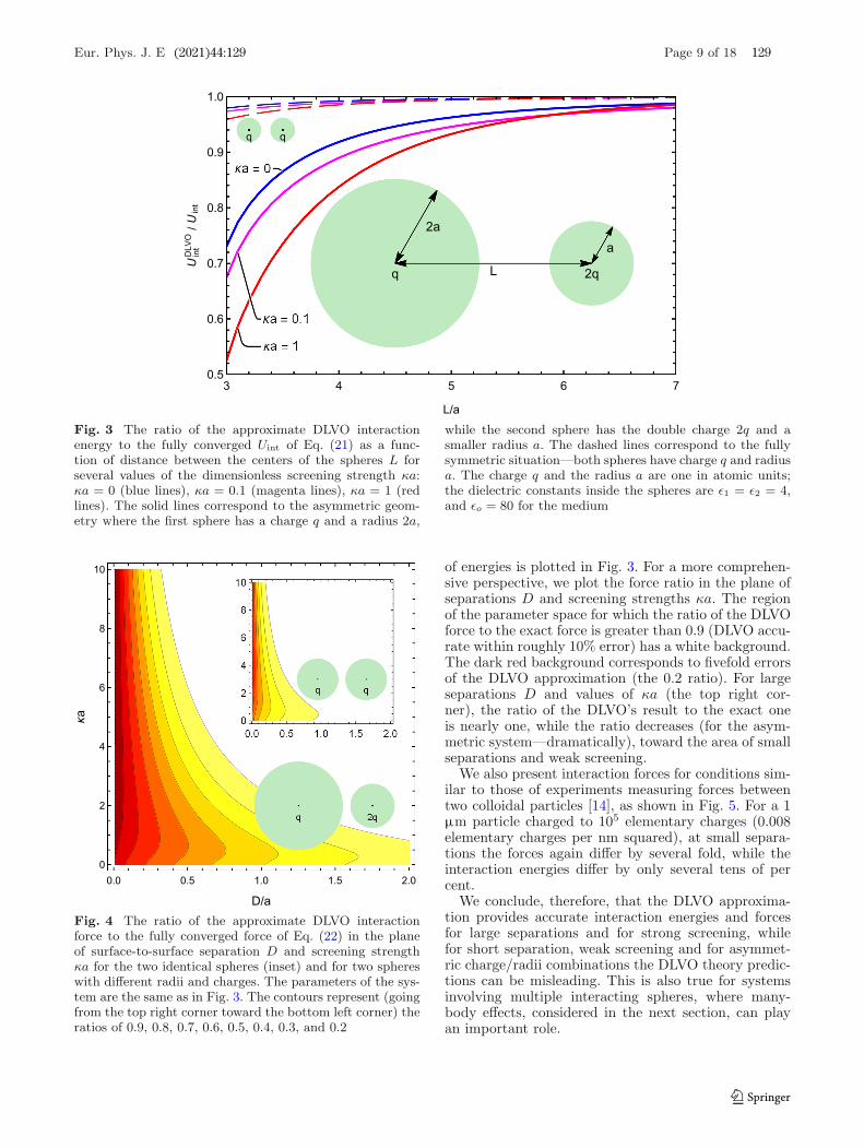
Fig. 3 The ratio of the approximate DLVO interactionenergy to the fully converged Uint of Eq. (21) as a func-tion of distance between the centers of the spheres L forseveral values of the dimensionless screening strength κa:κa = 0 (blue lines), κa = 0.1 (magenta lines), κa = 1 (redlines). The solid lines correspond to the asymmetric geom-etry where the first sphere has a charge q and a radius 2a,

while the second sphere has the double charge 2q and asmaller radius a. The dashed lines correspond to the fullysymmetric situation—both spheres have charge q and radiusa. The charge q and the radius a are one in atomic units;the dielectric constants inside the spheres are ε1 = ε2 = 4,and εo = 80 for the medium

Fig. 4 The ratio of the approximate DLVO interactionforce to the fully converged force of Eq. (22) in the planeof surface-to-surface separation D and screening strengthκa for the two identical spheres (inset) and for two sphereswith different radii and charges. The parameters of the sys-tem are the same as in Fig. 3. The contours represent (goingfrom the top right corner toward the bottom left corner) theratios of 0.9, 0.8, 0.7, 0.6, 0.5, 0.4, 0.3, and 0.2

of energies is plotted in Fig. 3. For a more comprehen-sive perspective, we plot the force ratio in the plane ofseparations D and screening strengths κa. The regionof the parameter space for which the ratio of the DLVOforce to the exact force is greater than 0.9 (DLVO accu-rate within roughly 10% error) has a white background.The dark red background corresponds to fivefold errorsof the DLVO approximation (the 0.2 ratio). For largeseparations D and values of κa (the top right cor-ner), the ratio of the DLVO’s result to the exact oneis nearly one, while the ratio decreases (for the asym-metric system—dramatically), toward the area of smallseparations and weak screening.

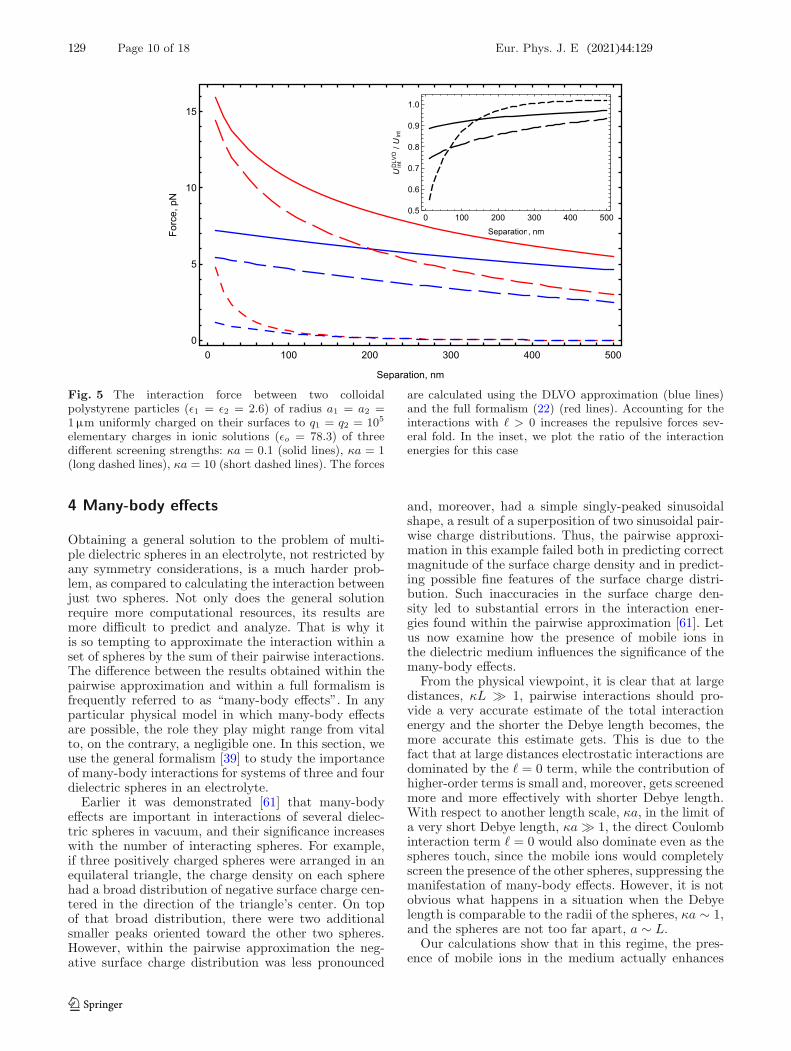
We also present interaction forces for conditions sim-ilar to those of experiments measuring forces betweentwo colloidal particles [14], as shown in Fig. 5. For a 1µm particle charged to 105 elementary charges (0.008elementary charges per nm squared), at small separa-tions the forces again differ by several fold, while theinteraction energies differ by only several tens of percent.

We conclude, therefore, that the DLVO approxima-tion provides accurate interaction energies and forcesfor large separations and for strong screening, whilefor short separation, weak screening and for asymmet-ric charge/radii combinations the DLVO theory predic-tions can be misleading. This is also true for systemsinvolving multiple interacting spheres, where many-body effects, considered in the next section, can playan important role.

123

129 Page 10 of 18 Eur. Phys. J. E (2021) 44:129

Fig. 5 The interaction force between two colloidalpolystyrene particles (ε1 = ε2 = 2.6) of radius a1 = a2 =1µm uniformly charged on their surfaces to q1 = q2 = 105

elementary charges in ionic solutions (εo = 78.3) of threedifferent screening strengths: κa = 0.1 (solid lines), κa = 1(long dashed lines), κa = 10 (short dashed lines). The forces

are calculated using the DLVO approximation (blue lines)and the full formalism (22) (red lines). Accounting for theinteractions with � > 0 increases the repulsive forces sev-eral fold. In the inset, we plot the ratio of the interactionenergies for this case

4 Many-body effects

Obtaining a general solution to the problem of multi-ple dielectric spheres in an electrolyte, not restricted byany symmetry considerations, is a much harder prob-lem, as compared to calculating the interaction betweenjust two spheres. Not only does the general solutionrequire more computational resources, its results aremore difficult to predict and analyze. That is why itis so tempting to approximate the interaction within aset of spheres by the sum of their pairwise interactions.The difference between the results obtained within thepairwise approximation and within a full formalism isfrequently referred to as “many-body effects”. In anyparticular physical model in which many-body effectsare possible, the role they play might range from vitalto, on the contrary, a negligible one. In this section, weuse the general formalism [39] to study the importanceof many-body interactions for systems of three and fourdielectric spheres in an electrolyte.

Earlier it was demonstrated [61] that many-bodyeffects are important in interactions of several dielec-tric spheres in vacuum, and their significance increaseswith the number of interacting spheres. For example,if three positively charged spheres were arranged in anequilateral triangle, the charge density on each spherehad a broad distribution of negative surface charge cen-tered in the direction of the triangle’s center. On topof that broad distribution, there were two additionalsmaller peaks oriented toward the other two spheres.However, within the pairwise approximation the neg-ative surface charge distribution was less pronounced

and, moreover, had a simple singly-peaked sinusoidalshape, a result of a superposition of two sinusoidal pair-wise charge distributions. Thus, the pairwise approxi-mation in this example failed both in predicting correctmagnitude of the surface charge density and in predict-ing possible fine features of the surface charge distri-bution. Such inaccuracies in the surface charge den-sity led to substantial errors in the interaction ener-gies found within the pairwise approximation [61]. Letus now examine how the presence of mobile ions inthe dielectric medium influences the significance of themany-body effects.

From the physical viewpoint, it is clear that at largedistances, κL 1, pairwise interactions should pro-vide a very accurate estimate of the total interactionenergy and the shorter the Debye length becomes, themore accurate this estimate gets. This is due to thefact that at large distances electrostatic interactions aredominated by the � = 0 term, while the contribution ofhigher-order terms is small and, moreover, gets screenedmore and more effectively with shorter Debye length.With respect to another length scale, κa, in the limit ofa very short Debye length, κa 1, the direct Coulombinteraction term � = 0 would also dominate even as thespheres touch, since the mobile ions would completelyscreen the presence of the other spheres, suppressing themanifestation of many-body effects. However, it is notobvious what happens in a situation when the Debyelength is comparable to the radii of the spheres, κa ∼ 1,and the spheres are not too far apart, a ∼ L.

Our calculations show that in this regime, the pres-ence of mobile ions in the medium actually enhances

123

Eur. Phys. J. E (2021) 44:129 Page 11 of 18 129

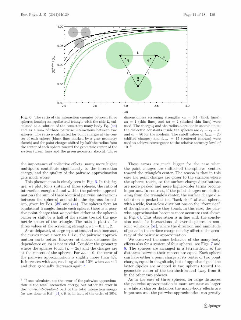
Fig. 6 The ratio of the interaction energies between threespheres forming an equilateral triangle with the side L, cal-culated as a solution of the consistent many-body Eq. (44)and as a sum of three pairwise interactions between twospheres. The ratio is calculated for point charges at the cen-ter of each sphere (black lines marked by a gray geometrysketch) and for point charges shifted by half the radius fromthe center of each sphere toward the geometric center of thesystem (green lines and the green geometry sketch). Three

dimensionless screening strengths κa = 0.1 (thick lines),κa = 1 (thin lines) and κa = 2 (dashed thin lines) wereused. The charge q and the radius a are one in atomic units;the dielectric constants inside the spheres are ε1 = ε2 = 4,and εo = 80 for the medium. The cutoff values of �max = 20(shifted charges) and �max = 15 (centered charges) wereused to achieve convergence to the relative accuracy level of10−3

the importance of collective effects, many more highermultipoles contribute significantly to the interactionenergy, and the quality of the pairwise approximationgets much worse.

This phenomenon is clearly seen in Fig. 6. In this fig-ure, we plot, for a system of three spheres, the ratio ofinteraction energies found within the pairwise approxi-mation (the sum of three identical pairwise interactionsbetween the spheres) and within the rigorous formal-ism, given by Eqs. (39) and (44). The spheres form anequilateral triangle. Inside each sphere, there is a posi-tive point charge that we position either at the sphere’scenter or shift by a half of the radius toward the geo-metric center of the triangle. The ratio is plotted forthree values of the screening strength, κa = 0.1, 1, 2.

As anticipated, at large separations and as κ increases,the curves move closer to 1, i.e., the pairwise approxi-mation works better. However, at shorter distances thedependence on κa is not trivial. Consider the geometrywhere the spheres touch (L = 2a) and the charges areat the centers of the spheres. For κa → 0, the error ofthe pairwise approximation is slightly more than 4%.It increases with κa, reaching about 10% when κa ∼ 1and then gradually decreases again.2

2 If one calculates not the error of the pairwise approxima-tion in the total interaction energy, but rather its error inthe non-point-Coulomb part of the total interaction energy(as was done in Ref. [61]), it is, in fact, of the order of 30%.

These errors are much bigger for the case whenthe point charges are shifted off the spheres’ centerstoward the triangle’s center. The reason is that in thiscase the point charges are closer to the surfaces wherethe spheres touch, so the surface charge distributionsare more peaked and more higher-order terms becomeimportant. In contrast, if the point charges are shiftedaway from the triangle’s center, the surface charge dis-tribution is peaked at the “back side” of each sphere,with a wide, featureless distributions on the “front side”of the spheres, where they touch. In this case, the pair-wise approximation becomes more accurate (not shownin Fig. 6). This observation is in line with the conclu-sion made for interactions of several spheres in non-ionic solutions [61], where the direction and amplitudeof peaks in the surface charge density affected the accu-racy of the pairwise approximation.

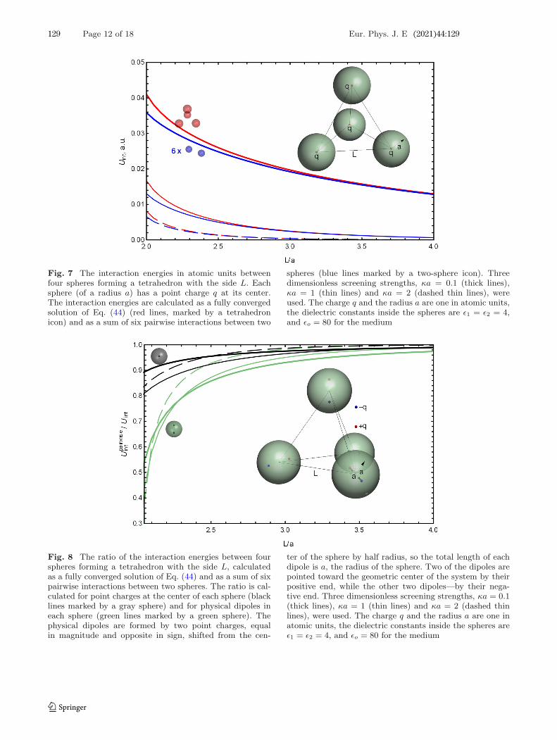
We observed the same behavior of the many-bodyeffects also for a system of four spheres, see Figs. 7 and8. The spheres are arranged in a tetrahedron, so thedistances between their centers are equal. Each spherecan have either a point charge at its center or two pointcharges, equal in magnitude, but of opposite signs. Thelatter dipoles are oriented in two spheres toward thegeometric center of the tetrahedron and away from itin the other two spheres.

As in the case of three spheres, for large distancesthe pairwise approximation is more accurate at largerκ, while at shorter distances the many-body effects areimportant and the pairwise approximation can greatly

123

129 Page 12 of 18 Eur. Phys. J. E (2021) 44:129

Fig. 7 The interaction energies in atomic units betweenfour spheres forming a tetrahedron with the side L. Eachsphere (of a radius a) has a point charge q at its center.The interaction energies are calculated as a fully convergedsolution of Eq. (44) (red lines, marked by a tetrahedronicon) and as a sum of six pairwise interactions between two

spheres (blue lines marked by a two-sphere icon). Threedimensionless screening strengths, κa = 0.1 (thick lines),κa = 1 (thin lines) and κa = 2 (dashed thin lines), wereused. The charge q and the radius a are one in atomic units,the dielectric constants inside the spheres are ε1 = ε2 = 4,and εo = 80 for the medium

Fig. 8 The ratio of the interaction energies between fourspheres forming a tetrahedron with the side L, calculatedas a fully converged solution of Eq. (44) and as a sum of sixpairwise interactions between two spheres. The ratio is cal-culated for point charges at the center of each sphere (blacklines marked by a gray sphere) and for physical dipoles ineach sphere (green lines marked by a green sphere). Thephysical dipoles are formed by two point charges, equalin magnitude and opposite in sign, shifted from the cen-

ter of the sphere by half radius, so the total length of eachdipole is a, the radius of the sphere. Two of the dipoles arepointed toward the geometric center of the system by theirpositive end, while the other two dipoles—by their nega-tive end. Three dimensionless screening strengths, κa = 0.1(thick lines), κa = 1 (thin lines) and κa = 2 (dashed thinlines), were used. The charge q and the radius a are one inatomic units, the dielectric constants inside the spheres areε1 = ε2 = 4, and εo = 80 for the medium

123

Eur. Phys. J. E (2021) 44:129 Page 13 of 18 129

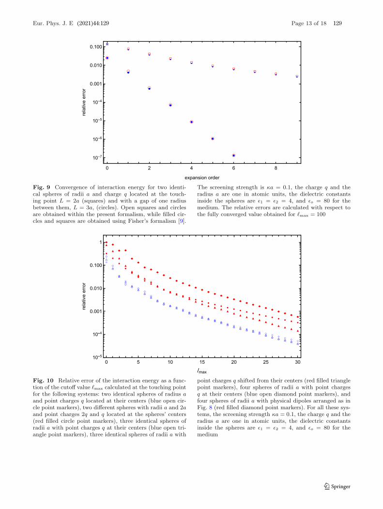
Fig. 9 Convergence of interaction energy for two identi-cal spheres of radii a and charge q located at the touch-ing point L = 2a (squares) and with a gap of one radiusbetween them, L = 3a, (circles). Open squares and circlesare obtained within the present formalism, while filled cir-cles and squares are obtained using Fisher’s formalism [9].

The screening strength is κa = 0.1, the charge q and theradius a are one in atomic units, the dielectric constantsinside the spheres are ε1 = ε2 = 4, and εo = 80 for themedium. The relative errors are calculated with respect tothe fully converged value obtained for �max = 100

Fig. 10 Relative error of the interaction energy as a func-tion of the cutoff value �max calculated at the touching pointfor the following systems: two identical spheres of radius aand point charges q located at their centers (blue open cir-cle point markers), two different spheres with radii a and 2aand point charges 2q and q located at the spheres’ centers(red filled circle point markers), three identical spheres ofradii a with point charges q at their centers (blue open tri-angle point markers), three identical spheres of radii a with

point charges q shifted from their centers (red filled trianglepoint markers), four spheres of radii a with point chargesq at their centers (blue open diamond point markers), andfour spheres of radii a with physical dipoles arranged as inFig. 8 (red filled diamond point markers). For all these sys-tems, the screening strength κa = 0.1, the charge q and theradius a are one in atomic units, the dielectric constantsinside the spheres are ε1 = ε2 = 4, and εo = 80 for themedium

123

129 Page 14 of 18 Eur. Phys. J. E (2021) 44:129

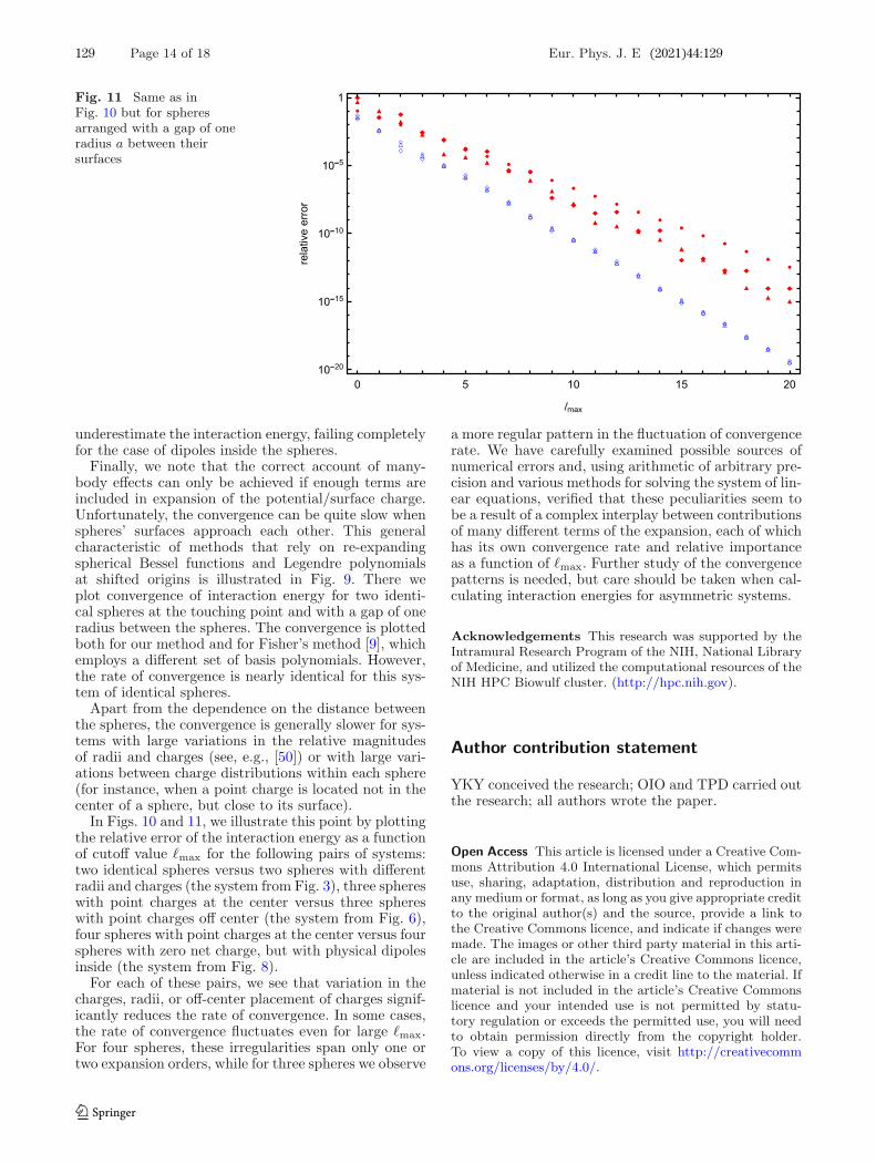
Fig. 11 Same as inFig. 10 but for spheresarranged with a gap of oneradius a between theirsurfaces

underestimate the interaction energy, failing completelyfor the case of dipoles inside the spheres.

Finally, we note that the correct account of many-body effects can only be achieved if enough terms areincluded in expansion of the potential/surface charge.Unfortunately, the convergence can be quite slow whenspheres’ surfaces approach each other. This generalcharacteristic of methods that rely on re-expandingspherical Bessel functions and Legendre polynomialsat shifted origins is illustrated in Fig. 9. There weplot convergence of interaction energy for two identi-cal spheres at the touching point and with a gap of oneradius between the spheres. The convergence is plottedboth for our method and for Fisher’s method [9], whichemploys a different set of basis polynomials. However,the rate of convergence is nearly identical for this sys-tem of identical spheres.

Apart from the dependence on the distance betweenthe spheres, the convergence is generally slower for sys-tems with large variations in the relative magnitudesof radii and charges (see, e.g., [50]) or with large vari-ations between charge distributions within each sphere(for instance, when a point charge is located not in thecenter of a sphere, but close to its surface).

In Figs. 10 and 11, we illustrate this point by plottingthe relative error of the interaction energy as a functionof cutoff value �max for the following pairs of systems:two identical spheres versus two spheres with differentradii and charges (the system from Fig. 3), three sphereswith point charges at the center versus three sphereswith point charges off center (the system from Fig. 6),four spheres with point charges at the center versus fourspheres with zero net charge, but with physical dipolesinside (the system from Fig. 8).

For each of these pairs, we see that variation in thecharges, radii, or off-center placement of charges signif-icantly reduces the rate of convergence. In some cases,the rate of convergence fluctuates even for large �max.For four spheres, these irregularities span only one ortwo expansion orders, while for three spheres we observe

a more regular pattern in the fluctuation of convergencerate. We have carefully examined possible sources ofnumerical errors and, using arithmetic of arbitrary pre-cision and various methods for solving the system of lin-ear equations, verified that these peculiarities seem tobe a result of a complex interplay between contributionsof many different terms of the expansion, each of whichhas its own convergence rate and relative importanceas a function of �max. Further study of the convergencepatterns is needed, but care should be taken when cal-culating interaction energies for asymmetric systems.

Acknowledgements This research was supported by theIntramural Research Program of the NIH, National Libraryof Medicine, and utilized the computational resources of theNIH HPC Biowulf cluster. (http://hpc.nih.gov).

Author contribution statement

YKY conceived the research; OIO and TPD carried outthe research; all authors wrote the paper.

Open Access This article is licensed under a Creative Com-mons Attribution 4.0 International License, which permitsuse, sharing, adaptation, distribution and reproduction inany medium or format, as long as you give appropriate creditto the original author(s) and the source, provide a link tothe Creative Commons licence, and indicate if changes weremade. The images or other third party material in this arti-cle are included in the article’s Creative Commons licence,unless indicated otherwise in a credit line to the material. Ifmaterial is not included in the article’s Creative Commonslicence and your intended use is not permitted by statu-tory regulation or exceeds the permitted use, you will needto obtain permission directly from the copyright holder.To view a copy of this licence, visit http://creativecommons.org/licenses/by/4.0/.

123

Eur. Phys. J. E (2021) 44:129 Page 15 of 18 129

Appendix A: Violation of reciprocity in thePoisson–Boltzmann framework

To provide context, we briefly review the discussions byOnsager [3] and McQuarrie [6] of the Poisson–Boltzmannand Debye–Huckel equations. For a neutral solution of pos-itive and negative ions in water (εo), these differential equa-

tions provide < φ(r, r1) >(1), the canonically averaged elec-tric potential at r while keeping a single ion fixed at r1.With φ ≡ ∑N

i=1 qi/(εo|r − ri|), one has

∇2 < φ(r, r1) >(1) = −4π

εo< ρ(r, r1) >(1) (24)

= −4π

εo

∑

s

csqsg1s (r, r1) (25)

≈ −4π

εo

∑

s

csqse−βqs<φ(r,r1)>(1)

(26)

Taking the square gradient of the expression for the canon-ical average of φ gives the first equality. The second equal-ity is by the definition of the radial distribution functiong1s(r, r1), where qs and cs are the charge and average con-centration of the ions of species s and β = 1/kBT is theinverse temperature. The final step is the approximationthat gives the well-known Poisson–Boltzmann equation:

∇2φ(r) = −4π

εo

∑

s

csqse−βqsφ(r) (27)

where we have without loss of generality set r1 = 0 andused streamlined notation for the potential in accordancewith common practice. Expanding the exponential to firstorder and noting that the zeroth-order term vanishes due tocharge neutrality gives the Debye–Huckel equation:

∇2φ(r) = κ2φ(r) (28)

where κ2 = 4π βεo

∑s csq

2s . However, we are not wedded to

this expression for κ. As noted by Fisher et al. [9], the rangeof validity and utility of the Debye–Huckel equation may beexpanded by considering κ to be a system parameter. Morerecently, Janacek and Netz [10] have performed numericalstudies that suggest the use of an effective screening param-eter κeff . The work of Alexander et al. [8] also suggests theexpanded applicability of Debye–Huckel theory when usingan effective κ.

Let us now consider some symmetry requirements. Gen-eralizing the above notation so that < φ(rk, rj) >(j) is thecanonically averaged electric potential at a point rk whilekeeping an ion fixed at point rj (and vice versa). By impos-ing translational symmetry and particle permutation sym-metry, the radial distribution function satisfies gjk(rj , rk) =gjk(|rj − rk|) = gkj(rk, rj). Note that the potential of mean

force w is defined via e−βwj,k(rj ,rk) ≡ gjk(rj , rk), implying

wj,k (rj , rk) = wk,j (rk, rj) . (29)

The reciprocity principle requires that the energy of thesystem be independent of the order in which it is assembled.Thus, one may bring ion k into position with ion j alreadyfixed or vice versa. The left-hand side above is the workrequired to bring ion j into position with ion k already fixed,

while the right-hand side corresponds to work required forbringing in ion k with ion j already fixed. Expressing thisin terms of the separation and taking the negative gradient,one sees that this is also an average form of Newton’s thirdlaw.

The approximation from (25) to (26) thus implies theneed of having

qj < φ(rj , rk) >(k)= qk < φ(rk, rj) >(j) , (30)

which is unlikely to hold when nonlinear terms are included.As Onsager stated, we have to expect the left-hand sidediffers from the right-hand side “except in very symmetriccases.” [3]

Interestingly, it is straightforward to verify that the solu-tion the the Debye–Huckel equation satisfies this require-ment. Moreover, this reciprocity has been explicitly proven[39] for the application of Debye–Huckel theory to an arbi-trary collection of dielectric spheres in solution.

Another symmetry requirement arises in the form of areciprocal relation. Since U = (1/2)

∑j qj

∑i qi/(εo|ri −

rj |), it is easy to see that:

∂F

∂qj= φj (31)

where F is the Helmholtz free energy and φj is the aver-age potential at rj (excluding the contribution from qj).Because the total differential of the electrostatic portion ofthe Helmholtz free energy is given by:

dF =∑

i

∂F

∂qidqi =

∑

i

φidqi, (32)

equality of the mixed partial derivatives implies:

∂φk

∂qj=

∂φj

∂qk(33)

Importantly, the solution to the Debye–Huckel equationsatisfies these requirements, but solutions to the Poisson–Boltzmann equation will not. Furthermore, it can be shown[5] that the Debye–Huckel equation is the exact small κ lim-iting form of Eq. (24). Evidently, the Debye–Huckel equa-tion has in some ways a firmer physical foundation than thePoisson–Boltzmann equation in spite of the fact that theformer is obtained as a linearization of the latter. Moreover,as Onsager [3] points out, “as soon as the higher terms in thePoisson–Boltzmann equation become important, we can nolonger expect the ionic atmospheres to be additive, and thenthe Poisson–Boltzmann equation itself becomes unreliable.”

A brief comment on van der Waals forces is perhapsappropriate at this point. The van der Waals interactionarises at the atomic scale as a result of quantum mechanicalfluctuations. Thus, the ions in an ionic solution might wellexperience van der Waals interactions. However, while theseforces are significant for atomic scale objects such as the ionsin the solution, it will generally not be the case for the muchlarger colloidal objects (macroions), which deserve a classi-cal approach. Nevertheless, this is not to say that there areno interactions of the form r−6 among colloidal particles. Anexpansion in inverse powers of the separation r of the elec-trostatic interaction of polarizable objects in a polarizablemedium will certainly include terms such as r−6 [61], buttheir origin lies in continuum macroscopic electrostatics.

123

129 Page 16 of 18 Eur. Phys. J. E (2021) 44:129

Appendix B: Recapitulation of general for-malism for arbitrary number of spheres

To make the presentation self-contained, let us provide hereall of the definitions and equations [39] necessary for cal-culating the interaction energy for a system of arbitrarynumber of dielectric spheres immersed in an ionic fluid.

The total electrostatic energy of the system, U , isobtained via sums of weighted products of Q�m, the spher-

ical components of free charge distributions, and Q+�m, the

spherical components of the net charge distributions thatinclude charges induced on the surfaces of the spheres [39]:

U =κ

2

N∑

k=1

∑

�m

[i�(κak) k�(κak) Q

k ∗�m Qk+

�m − 1

εk κak

Qk∗�m Q

k�m

(2� + 1)

]

+κ

2

N∑

k=1

∑

j �=k

∑

�m

∑

�1m1

(−1)�1

H�m�1m1(κLk→j) i�(κak) i�1(κaj) Qk∗�mQj+

�1m1. (34)

Here k (and j) enumerate the N spheres of radii ak (aj)and dielectric constants εk (εj), Lk→j is a vector connectingthe center of sphere k to that of sphere j, κ is the inverseDebye length, Y�m(r) are the standard spherical harmonicswith � ∈ [0, ∞), m ∈ [−�, �], i�(z) are the modified sphericalBessel functions of the first kind with i�(z) = (i)−�j�(i z),while k�(z) are the modified spherical Bessel functions of

the second kind with k�(z) = −(i)�h(1)� (i z).

The function H�m�1m1(κLk→j) takes care of different ori-gins when expanding the surface charges around the centerof each sphere:

H�m�1m1 (κLk→j) =∑

�2m2

H�1m1�m�2m2

k�2 (κLk→j) Y�2m2

(Lk→j

),

(35)

where

H�1m1�m�2m2

≡ C�1 0� 0 �2 0 C�1m1

� m �2m2

√4π

2�1 + 1

√(2� + 1)(2�2 + 1) ,

(36)

and C�1m1� m �2m2

are the Clebsch–Gordan coefficients. Note

that C�10� 0 �20 = 0 only if � + �1 + �2 is even. Therefore, the

sum in Eq. (35) should be taken only over �2 of the sameparity as � + �1. This condition on the parity of the sum ofthe angular momenta leads to other useful relations such as(−1)�1 = (−1)�+�2 .

The spherical components Qk

�m represent the free chargedistribution on each sphere and are connected with the cor-responding multipole moments q �m as:

Q�m ≡√

4πq �m

a�=

√4π

a�

∫ρ(s ) s� Y ∗

�m(s) ds. (37)

These spherical components are surface equivalents of ordi-nary multipoles, and the rigorous equivalence of using eitherthe ordinary multipoles or their surface equivalents has beendemonstrated, both with ions [39] and without ions [54].For convenience, the surface representation was used. Inthis case, the potential inside each sphere is a solution ofthe Laplace equation. The quantities Qk+

�m are a scaled ver-sion of the spherical components of the net (free + induced)

charge distributions, Qk�m, that are solved for when there

are no free ions in the dielectric medium [55]. The two setsof coefficients are connected via the following substitutionrule:

Qk+�m =

Qk�m

κak (2� + 1) i�(κak) k�(κak). (38)

The spherical components of the scaled net charge Qk+�m are

determined by the corresponding boundary conditions onthe surfaces of the spheres that result in the following systemof linear equations [39]:

Qk

�m = i�(κak) k�(κak) K(�, κak) Qk+�m

+∑

j �=k

∑

�1m1

(−1)�1 i�(κak) i�1(κaj) I(�, κak)

H�m�1m1(κLk→j) Qj+�1m1

, (39)

where, for the sake of compactness, we introduced the fol-lowing notations:

K (�, κak) ≡ κak

[� εk − κak k′

� (κak)

k� (κak)εo

], I (�, κak)

≡ κak

[� εk − κak i′� (κak)

i� (κak)εo

]. (40)

One can avoid using derivatives of the modified sphericalBessel functions by employing the following equalities:

k′�(x) =

� k�(x)

x− k�+1(x), i′�(x) =

� i�(x)

x+ i�+1(x),

(41)

so that

K(�, κak) = κak

[�(εk − εo) +

κak k�+1(κak)

k�(κak)εo

],

I(�, κak) = κak

[�(εk − εo) − κak i�+1(κak)

i�(κak)εo

]. (42)

System (39), of course, is of infinite size, and the seriesin � must be terminated at some �max, leaving N(�max +1)2

equations. A significant advantage of the formalism [39] isthat there is only one parameter, namely �max, that governsthe accuracy of the obtained result. In contrast, termina-tion of another expansion is necessary in the formalism ofRef. [49], while in Ref. [56], transposing the origin of spher-ical waves expansion is designed as a recursive procedure.Introducing such extra cut-offs complicates verification ofthe achieved accuracy.

An analysis of convergence of the electrostatic energy as afunction of increasing �max has been carried out in Ref. [39].For two spheres of comparable sizes and charges, �max = 10is sufficient for achieving relative error of 10−8 almost tothe distance where the spheres touch (the so-called touchingpoint). However, as we will see below, when there is variationin sphere radii or charge magnitude or placement, the valueof �max should be set higher.

In order to get the interaction energy, one has to subtractthe sum of solvation energies of each sphere. The multipolecomponents of the solvation energies are given [39] as:

Usolv =κ

2

∑

�m

[2� + 1

K(�, κa)− 1

ε κa

]Q

∗�m Q�m

(2� + 1). (43)

123

Eur. Phys. J. E (2021) 44:129 Page 17 of 18 129

Thus,

Uint =κ

2

N∑

k=1

∑

�m

[i�(κak) k�(κak) Q

k∗�m Qk+

�m − Qk∗�m Q

k�m

K(�, κak)

]

+κ

2

N∑

k=1

∑

j �=k

∑

�m

∑

�1m1

(−1)�1 H�m�1m1 (κLk→j) i� (κak) i�1

(κaj) Qk∗�mQj+

�1m1. (44)

Finally, let us note that in the limit of κ → 0 (no mobileions in the solvent), the presented formalism reduces to theformalism of dielectric spheres in a dielectric medium [55],as shown in Ref. [39].

References

1. L. Onsager, Physik. Z. 28, 277 (1927)2. R.H. Fowler, Trans. Faraday Soc. 23, 434 (1927)3. L. Onsager, Chem. Rev. 13, 73 (1933)4. J.G. Kirkwood, J.C. Poirier, J. Phys. Chem. 58, 591

(1954)5. W. Oivares, D.A. McQuarrie, Biophys. J. 15, 143 (1975)6. D.A. McQuarrie, Statistical Mechanics (Harper & Row,

1976)7. P. Debye, E. Huckel, Phys. Z. 24, 185 (1923). https://

doi.org/10.1007/978-3-642-94260-0_98. S. Alexander, P.M. Chaikin, P. Grant, G.J. Morales, P.

Pincus, D. Hone, J. Chem. Phys. 80, 5776 (1984)9. M.E. Fisher, Y. Levin, X. Li, J. Chem. Phys. 101(3),

2273 (1994). https://doi.org/10.1063/1.46766810. J. Janacek, R.R. Netz, J. Phys. Chem. 130, 074502

(2009)11. E. Trizac, L. Bocquet, M. Aubouy, H.H. von Grunberg,

Langmuir 19, 4027 (2003)12. R.R. Netz, H. Orland, Europhys. Lett. 45, 726 (1999)13. L.M. Varela, M. Garcıa, V. Mosquera, Phys. Rep. 382,

1 (2003)14. C. Gutsche, U. Keyser, F. Kremer, P. Linse, Langmuir

76, 031403 (2007)15. J.G. Kirkwood, J. Chem. Phys. 2(7), 351 (1934).

https://doi.org/10.1063/1.174948916. H. Kallmann, M. Willstaetter, Die Naturwis-

senschaften 20(51), 952 (1932). https://doi.org/10.1007/BF01504717

17. H.C. Hamaker, Physica 4(10), 1058 (1937). https://doi.org/10.1016/S0031-8914(37)80203-7

18. I. Langmuir, J. Chem. Phys. 6(12), 873 (1938). https://doi.org/10.1063/1.1750183

19. B. Derjaguin, Trans. Faraday Soc. 35, 203 (1940).https://doi.org/10.1039/TF9403500203

20. F. London, As cited in paper by S. Levine and G. P.Dube in Trans. Farady Soc. 35, 1125 (1935)

21. S. Levine, G.P. Dube, Trans. Faraday Soc. 35, 1125(1939). https://doi.org/10.1039/TF9393501125

22. B. Derjaguin, L. Landau, Acta Phys. U.R.S.S. 14, 633(1941)

23. B. Derjaguin, L. Landau, Progr. Surf. Sci. 43(1–4), 30(1993). https://doi.org/10.1016/0079-6816(93)90013-l

24. E. Verwey, J. Overbeek, Theory of the Stability ofLyophobic Colloids (Elsevier, Amsterdam, 1948)

25. E. Verwey, J. Overbeek, J. Colloid Sci. 10(2), 224(1955). https://doi.org/10.1016/0095-8522(55)90030-1

26. F.J.M. Ruiz-Cabello, P. Maroni, M. Borkovec, J. Chem.Phys. 138(23), 234705 (2013). https://doi.org/10.1063/1.4810901

27. H.W. Cho, M.L. Mugnai, T.R. Kirkpatrick, D. Thiru-malai, Phys. Rev. E 101, 032605 (2020)

28. J. Qin, J. Li, V. Lee, H. Jaeger, J.J. de Pablo, K.F.Freed, J. Colloid Interface Sci. 469, 237 (2016). https://doi.org/10.1016/j.jcis.2016.02.033

29. H. Ohshima, J. Colloid Interface Sci. 170(2), 432 (1995).https://doi.org/10.1006/jcis.1995.1122

30. X. Chu, D.T. Wasan, J. Colloid Interface Sci. 184(1),268 (1996). https://doi.org/10.1006/jcis.1996.0620

31. E.B. Lindgren, C. Quan, B. Stamm, J. Chem.Phys. 150(4), 044901 (2019). https://doi.org/10.1063/1.5079515

32. A.V. Filippov, J. Exp. Theor. Phys. 109(3), 516 (2009).https://doi.org/10.1134/S1063776109090179

33. C. Berti, D. Gillespie, J.P. Bardhan, R.S. Eisenberg,C. Fiegna, Phys. Rev. E Stat. Nonlinear Soft MatterPhys. 86(1), 011912 (2012). https://doi.org/10.1103/PhysRevE.86.011912

34. K. Barros, D. Sinkovits, E. Luijten, J. Chem.Phys. 140(6), 064903 (2014). https://doi.org/10.1063/1.4863451

35. L. Li, C. Li, S. Sarkar, J. Zhang, S. Witham, Z. Zhang, L.Wang, N. Smith, M. Petukh, E. Alexov, BMC Biophys.5, 9 (2012). https://doi.org/10.1186/2046-1682-5-9

36. P. Koehl, Curr. Opin. Struct. Biol. 16(2), 142 (2006).https://doi.org/10.1016/j.sbi.2006.03.001

37. Z. Gan, Z. Wang, S. Jiang, Z. Xu, E. Luijten, J. Chem.Phys. 151(2), 024112 (2019)

38. S. Nordholm, J. Chem. Phys. 78(9), 5759 (1983).https://doi.org/10.1063/1.445459

39. Y.K. Yu, Phys. Rev. E 102(5), 052404 (2020). https://doi.org/10.1103/PhysRevE.102.052404

40. I.N. Derbenev, A.V. Filippov, A.J. Stace, E. Besley, J.Chem. Phys. 152(2), 024121 (2020). https://doi.org/10.1063/1.5129756

41. N. Hoffmann, C.N. Likos, J.P. Hansen, Mol. Phys. 102,857 (2004)

42. N. Boon, E. Carvajal Gallardo, S. Zheng, E. Eggen, M.Dijkstra, R. van Roij, J. Phys. Condens. Matter 22,104104 (2010)

43. J. de Graaf, N. Boon, M. Dijkstra, R. van Roij, J. Chem.Phys. 137, 104910 (2012)

44. C. Russ, H.H. von Grunberg, M. Dijkstra, R. van Roij,Phys. Rev. E 66, 011402 (2002)

45. N.V. Sushkin, G.D. Phillies, J. Chem. Phys. 103(11),4600 (1995). https://doi.org/10.1063/1.470647

46. E. Bichoutskaia, A.L. Boatwright, A. Khachatourian,A.J. Stace, J. Chem. Phys. 133(2), 024105 (2010).https://doi.org/10.1063/1.3457157

47. A.J. Stace, A.L. Boatwright, A. Khachatourian, E.Bichoutskaia, J. Colloid Interface Sci. 354(1), 417(2011). https://doi.org/10.1016/j.jcis.2010.11.030

48. A. Khachatourian, H.K. Chan, A.J. Stace, E. Bichout-skaia, J. Chem. Phys. 140(7), 074107 (2014). https://doi.org/10.1063/1.4862897

49. I.N. Derbenev, A.V. Filippov, A.J. Stace, E. Besley, J.Chem. Phys. 145(8), 084103 (2016)

50. E.B. Lindgren, H.K. Chan, A.J. Stace, E. Besley, Phys.Chem. Chem. Phys. 18(8), 5883 (2016). https://doi.org/10.1039/c5cp07709e

123

129 Page 18 of 18 Eur. Phys. J. E (2021) 44:129

51. I.N. Derbenev, A.V. Filippov, A.J. Stace, E. Besley, SoftMatter 14(26), 5480 (2018). https://doi.org/10.1039/C8SM01068D

52. T.P. Doerr, Y.K. Yu, Phys. Rev. E Stat. Nonlinear SoftMatter Phys. 73(6), 061902 (2006). https://doi.org/10.1103/PhysRevE.73.061902

53. O. Obolensky, T. Doerr, R. Ray, Y.K. Yu, Phys. Rev. EStat. Nonlinear Soft Matter Phys. 79(4), 041907 (2009).https://doi.org/10.1103/PhysRevE.79.041907

54. T. Doerr, O. Obolensky, Y.K. Yu, Phys. Rev. E 96(6),062414 (2017). https://doi.org/10.1103/PhysRevE.96.062414

55. Y.K. Yu, Phys. Rev. E 100(1), 012401 (2019). https://doi.org/10.1103/PhysRevE.100.012401

56. I. Lotan, T. Head-Gordon, J. Chem. Theory Comput.2(3), 541 (2006). https://doi.org/10.1021/ct050263p

57. T.P. Doerr, Y.K. Yu, Am. J. Phys. 82(5), 460 (2014).https://doi.org/10.1119/1.4869281

58. D. Varshalovich, N. Moskalev, V. Khersonskii, QuantumTheory of Angular Momentum (World Scientific Pub-lishing Co, Singapore, 1988)

59. F. Naderi Mehr, D. Grigoriev, R. Heaton, J. Baptiste,A.J. Stace, N. Puretskiy, E. Besley, A. Boker, Small16(14), 2000442 (2020). https://doi.org/10.1002/smll.202000442

60. B. Stojimirovic, M. Vis, R. Tuinier, A.P. Philipse, G.Trefalt, Langmuir 36, 47 (2020)

61. O.I. Obolensky, T.P. Doerr, A.Y. Ogurtsov, Y.K. Yu,Europhys. Lett. 116(2), 24003 (2016). https://doi.org/10.1209/0295-5075/116/24003

123