Research Collection

Conference Paper

Structural equations modelling of travel behaviour dynamicsusing a pseudo panel approach

Author(s): Axhausen, Kay W.; Weis, Claude

Publication Date: 2009

Permanent Link: https://doi.org/10.3929/ethz-a-005919197

Rights / License: In Copyright - Non-Commercial Use Permitted

This page was generated automatically upon download from the ETH Zurich Research Collection. For moreinformation please consult the Terms of use.

ETH Library

Structural Equations Modelling of Travel

Behaviour Dynamics Using a Pseudo Panel

Approach

Claude Weis, IVT, ETH Zurich, Switzerland; Kay W. Axhausen,

IVT, ETH Zurich, Switzerland

Abstract Induced traffic has been a topic of research for many

years. While previous studies have focused on specific and

localised changes, the research described in this paper deals with

aggregate effects of changed generalised costs of travel on traffic

generation: the propensity of participating in out-of-home activities

on a given day, the number of trips and journeys conducted, and

the resulting total times out-of-home and distances travelled. Thus,

induced traffic is defined as additional demand generated by

improvements in travel conditions. The generalised cost elasticities

computed from a structural equations model with a pseudo panel

constructed from the Swiss National Travel Survey datasets are

surprisingly substantial even after correcting for socio-

demographic effects.

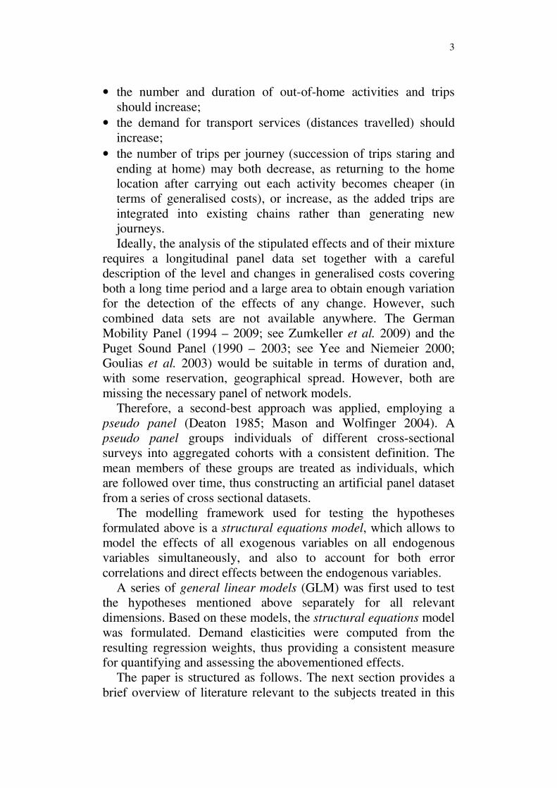
1. Motivation

Induced traffic has been a topic of ongoing research for many

years, the main focus being the assessment of side effects of

measures bringing about such improvements. While previous

studies have focused on specific and localised changes, the

research described in this paper deals with the aggregate effects of

changing generalised costs of travel on traffic generation: the

propensity of participating in out-of-home activities, or being

mobile on a given day, the number of trips conducted, and the

resulting total times spent out-of-home and distances travelled.

Generalised cost is understood as the risk- and comfort-weighted

sum of resources consumed for travel: time and (decision-relevant)

monetary expenditures. Thus, the phenomenon of induced traffic is

2

here defined as additional demand for transport services directly

caused by improving travel conditions.

The objective of the recently finished project work (Weis and

Axhausen 2009) that this paper draws on was to overcome the

limitations of previous studies (see next section) by addressing the

issue over a longer time period and a wider spatial scale than usual.

Accessibility is used as the central explanatory variable, as it is

equally important in policy discussions around transport projects

and policy making. It is an overall measure of the quality of service

offered by the transport system. It is assumed that travel is a

normal good (Varian 1992) – travellers respond to changes in

generalised costs of travel by adapting their consumption.

Individuals can adapt their travel behaviour (see Axhausen 2008

for a classification of movement into consistent elements) on

several levels:

• deciding to leave home and to participate in out-of-home

activities on a given day;

• adapting of the number of out-of-home activities;

• combining out-of-home activities and trips into tours (journeys)

or trip chains;

• scheduling (timing and duration) the activities;

• choosing the locations for carrying out activities (destination

choice);

• choosing an origin-destination connection (mode and route

choice) to reach the destination.

As the number of existing studies dealing with the latter two

dimensions (which represent the second to fourth steps in the

classic four step model, see Ortúzar and Willumsen 2001) is large,

and the scheduling process very locally specific and personal, this

paper focuses on an aggregate analysis of the upper levels, which

constitute the demand generation process. The scheduling process

and the intra-household interaction issue are being addressed in

ongoing work through a stated adaptation survey following the

tradition of the Household Activity Travel Survey (HATS; see

Jones et al. 1980).

When generalised costs sink, both the time and the monetary

resources for participating in travel and non-travel activities

increase. It is reasonable to expect that this shift in resource

availability will lead to a number of demand generation responses:

• the propensity of participating in out-of-home activities should

increase;

3

• the number and duration of out-of-home activities and trips

should increase;

• the demand for transport services (distances travelled) should

increase;

• the number of trips per journey (succession of trips staring and

ending at home) may both decrease, as returning to the home

location after carrying out each activity becomes cheaper (in

terms of generalised costs), or increase, as the added trips are

integrated into existing chains rather than generating new

journeys.

Ideally, the analysis of the stipulated effects and of their mixture

requires a longitudinal panel data set together with a careful

description of the level and changes in generalised costs covering

both a long time period and a large area to obtain enough variation

for the detection of the effects of any change. However, such

combined data sets are not available anywhere. The German

Mobility Panel (1994 – 2009; see Zumkeller et al. 2009) and the

Puget Sound Panel (1990 – 2003; see Yee and Niemeier 2000;

Goulias et al. 2003) would be suitable in terms of duration and,

with some reservation, geographical spread. However, both are

missing the necessary panel of network models.

Therefore, a second-best approach was applied, employing a

pseudo panel (Deaton 1985; Mason and Wolfinger 2004). A

pseudo panel groups individuals of different cross-sectional

surveys into aggregated cohorts with a consistent definition. The

mean members of these groups are treated as individuals, which

are followed over time, thus constructing an artificial panel dataset

from a series of cross sectional datasets.

The modelling framework used for testing the hypotheses

formulated above is a structural equations model, which allows to

model the effects of all exogenous variables on all endogenous

variables simultaneously, and also to account for both error

correlations and direct effects between the endogenous variables.

A series of general linear models (GLM) was first used to test

the hypotheses mentioned above separately for all relevant

dimensions. Based on these models, the structural equations model

was formulated. Demand elasticities were computed from the

resulting regression weights, thus providing a consistent measure

for quantifying and assessing the abovementioned effects.

The paper is structured as follows. The next section provides a

brief overview of literature relevant to the subjects treated in this

4

paper. The subsequent sections describe the construction of the

pseudo panel dataset, the variables it contains, an explorative

analysis of the pseudo panel and its variation over time, and the

model formulation and estimation steps, followed by

considerations on the application of the model results, a brief

conclusion and an outlook on further work.

2. Literature Overview

Fröhlich (2003) provides a literature review of models treating the

effects of increased road supply. All of these studies deal with the

classic definition of induced traffic, namely the reaction of demand

for transport services (travel times and distances) to the

improvement of the capacities of the transport system and the

implied drops in generalised travel costs. Goodwin (1992, 1996),

Noland and Levinson (2000), Graham and Glaister (2004) and

Goodwin et al. (2004) provide overviews of known income, price

and supply elasticities of car ownership and demand for transport

services, measured in vehicle miles travelled. Similar analyses can

be found in the works of Oum (1992), Cerwenka and Hauger

(1996), Cairns et al. (1998) de Corla-Souza and Cohen (1999), Lee

et al. (1999), Barr (2000), Fulton et al. (2000), Noland and Cowart

(2000), Noland (2001) and Cervero and Hansen (2002).

Swiss studies dealing with traffic induced by localised changes

to the transport system and the according accessibility changes

include Sommer et al. (2004), Güller et al. (2004) Giacomazzi et

al. (2004) and Aliesch et al. (2006), providing ex-post analyses of

the effects of the implementation of various road and rail projects.

The mentioned analyses remain vague in their conclusions. Like all

ex-post analyses, they suffer from the enormous challenges

imposed by the empirical data requirements. In order to provide a

detailed assessment of induced travel effects, all re-routed trips

would have to be recorded before and after the implementation of

the measure under study. Rudel and Maggi (2007) present current

results based on the analysis of potential mobility pricing schemes.

The effects of the structural changes of the aggregate system are

the subject of three recently completed dissertations at the Institute

for Transport Planning and Systems (IVT, ETH Zurich). The

studies are partly based on the same data employed here – the

5

Swiss network models for private and public transport (Fröhlich et

al. 2005), updated once a decade since 1950, and a detailed

database of Swiss municipalities since 1950 which was enriched

with spatial and welfare data (Tschopp et al. 2003). Fröhlich

(2008) uses the data for modelling the development of commuting

behaviour since 1970. Tschopp et al. (2005) (as well as Tschopp

2007) analyse the influence of changes in the transport system and

the corresponding accessibilities on the numbers of residents and

workers in the municipalities. Bodenmann (2007) provides an

analysis of the interaction of firm locations and the transport

system since 1970.

Literature dealing with the demand dimensions that are

discussed in this paper is quite sparse, indicating that the

generation side of transport demand has been neglected during the

past years. Meier (1989) makes an early attempt at explaining

general induced travel demand effects in Switzerland, among

others by analysing the variation of mobility (expressed by the

share of mobiles and number of trips) by accessibility (in classes)

and showing higher mobility for regions with superior

accessibility. Other examples that draw on concepts similar to

those employed here include Kumar and Levinson (1992), the

investigation of a generation model for work and non-work trips;

Madre et al. (2004), a meta analysis of immobility in travel diary

surveys; Mokhtarian and Chen (2004), a literature review of

studies discussing the concept of constant travel time budget; van

Wee et al. (2006), a quest for an explanation of increasing total

daily travel times; Primerano et al. (2008), where definitions for

trip chaining behaviour are provided.

3. Pseudo Panel Dataset Construction

The concept of pseudo panel data, first introduced by Deaton

(1985), consists in grouping individuals from cross sectional

observations into cohorts, the averages of which are then treated as

individual observations in an artificial panel. These data can be

used in the absence of actual panel data to approximate the latter

by following virtual persons (created by the aggregation into

cohorts; Mason and Wolfinger 2004) over time and test for

individual as well as dynamic effects. The approach has seen

6

common use in the transport planning field in recent years. An

example for its application is Bush (2003), an effort to forecast

future travel demand of baby boomers. Similar concepts underlie

the works by Goulias et al. (2007), Dargay (2002, 2007) and

Huang (2007), where evidence for the substantial influence of

cohort effects on household car ownership is provided.

The pseudo panel dataset for the present study was constructed

using the Swiss National Travel Survey (named Microcensus) data,

a person-based survey. In general only one person per household is

interviewed. The survey has been carried out approximately every

5 years since 1974. Over the course of time, survey methods have

changed several times, complicating the comparison of the

resulting data. A brief overview of the various surveys is given in

Table 1 (adapted from Simma 2003), along with the sample sizes

(number of surveyed households).

Table 1 Key Characteristics of Swiss Microcensus Travel Surveys Since 1974

Year Survey method Sample size

1974 Time use surveys 2’114

1979 Combination of pen-and-paper and personal interview 2’000

1984 Trip based diary 3’513

1989 Pen-and-paper survey 20’472

1994 16’570

2000 28’054

2005

Stage based diary

CATI

31’950

Source: Simma (2003)

As the different survey methods lead to discrepancies in the

data, the various household, person and travel datasets had to

undergo a thorough reformatting in order to obtain a uniform data

format for all persons over the different years and a consistent

coding for the relevant socio-demographic characteristics and

especially for the key mobility indicators (trip numbers et cetera).

For example, a severe decrease in reported mobility (as far as

increased non-mobility as well as reduced trip numbers are

concerned) is obvious in the 1989 dataset (Simma 2003). This

discrepancy appears not to be explicable by mere seasonal

fluctuations, but rather related to an underreporting of trips in the

7

corresponding trip diary. These effects, which are likely to be

artefacts of survey methods or the fieldwork in the relevant year,

are taken into account and corrected for in the modelling

procedures that will be discussed in the following sections. Lleras

et al. (2003) present approaches to account for data inconsistencies

across travel behaviour surveys in pooled analyses.

The cohorts for the pseudo panel dataset ought to be constructed

according to characteristics that are (or can reasonably be assumed

to be) time invariant. The most obvious example of such a

discriminating variable is the year of birth (which has been used in

multiple studies, such as Dargay 2002; Huang 2007). Other

criteria, such as gender, education level, or spatial characteristics,

are also conceivable as grouping variables.

When constructing a pseudo panel, two conflicting aims ought

to be met: on the one hand, the cohorts should be constructed in a

way that provides sufficient variability in the panel and provides a

sufficient number of artificially constructed observations in order

to estimate robust models. Thus, the cohort definition should be as

detailed as possible. On the other hand though, when the

disaggregation level becomes too detailed, the number of

observations per cohort will become small for certain time periods,

leading to greater weights of potential outliers in computing the

cohort averages and thus to biased estimates of the population

means (Huang 2007).

As a compromise between a sufficient level of disaggregation

and large enough cohort sizes, a cohort subdivision according to

three criteria was chosen:

• year of birth (split up into 10 year bands ranging from 1896

through 1985);

• gender;

• region (one out of 7 Swiss regions; the aggregation corresponds

to the EU NUTS 2 regions; Eurostat 2008).

The latter was chosen over a spatial definition based on

municipality types (urban, suburban, rural, et cetera). Such a

classification would be teleological and bias the results, as it can be

argued that relocations to better accessible places of residence (to a

different municipality type) take place because of a certain desired

mobility behaviour. The postulated direct causal effect of

accessibility on trip generation would then not be discernible from

a confounding residential self selection effect (Boarnet and Crane

2004; Mokhtarian and Cao 2008).

8

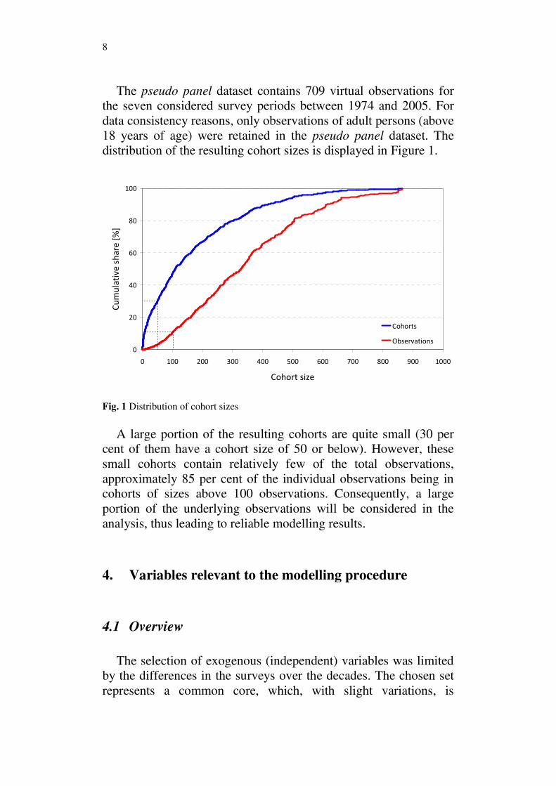
The pseudo panel dataset contains 709 virtual observations for

the seven considered survey periods between 1974 and 2005. For

data consistency reasons, only observations of adult persons (above

18 years of age) were retained in the pseudo panel dataset. The

distribution of the resulting cohort sizes is displayed in Figure 1.

0

20

40

60

80

100

0 100 200 300 400 500 600 700 800 900 1000

Cohort size

Cu

mu

lati

ve

sh

are

[%

]

Cohorts

Observations

Fig. 1 Distribution of cohort sizes

A large portion of the resulting cohorts are quite small (30 per

cent of them have a cohort size of 50 or below). However, these

small cohorts contain relatively few of the total observations,

approximately 85 per cent of the individual observations being in

cohorts of sizes above 100 observations. Consequently, a large

portion of the underlying observations will be considered in the

analysis, thus leading to reliable modelling results.

4. Variables relevant to the modelling procedure

4.1 Overview

The selection of exogenous (independent) variables was limited

by the differences in the surveys over the decades. The chosen set

represents a common core, which, with slight variations, is

9

regularly used in models of travel behaviour (Dargay 2002; Bush

2003; Huang 2007). The averages for those variables expected to

have an impact on the mobility indicators to be modelled were

computed.

Furthermore, the dataset was enriched with variables that,

individually or in combination, may be used as a proxy for

generalised costs of mobility tool ownership, respectively travel:

• accessibility measures (Tschopp et al 2005; Fröhlich 2008);

• price indices for individual travel (Abay 2000; values up to 2005

were extrapolated).

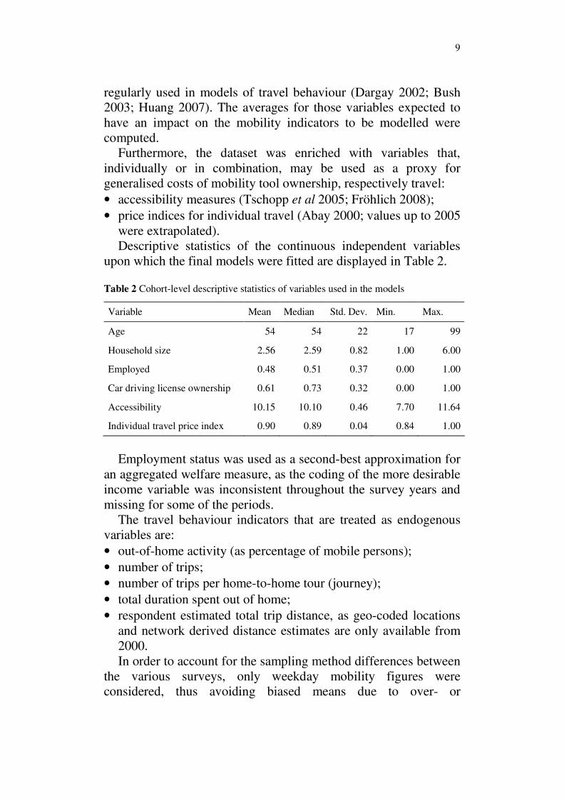
Descriptive statistics of the continuous independent variables

upon which the final models were fitted are displayed in Table 2.

Table 2 Cohort-level descriptive statistics of variables used in the models

Variable Mean Median Std. Dev. Min. Max.

Age 54 54 22 17 99

Household size 2.56 2.59 0.82 1.00 6.00

Employed 0.48 0.51 0.37 0.00 1.00

Car driving license ownership 0.61 0.73 0.32 0.00 1.00

Accessibility 10.15 10.10 0.46 7.70 11.64

Individual travel price index 0.90 0.89 0.04 0.84 1.00

Employment status was used as a second-best approximation for

an aggregated welfare measure, as the coding of the more desirable

income variable was inconsistent throughout the survey years and

missing for some of the periods.

The travel behaviour indicators that are treated as endogenous

variables are:

• out-of-home activity (as percentage of mobile persons);

• number of trips;

• number of trips per home-to-home tour (journey);

• total duration spent out of home;

• respondent estimated total trip distance, as geo-coded locations

and network derived distance estimates are only available from

2000.

In order to account for the sampling method differences between

the various surveys, only weekday mobility figures were

considered, thus avoiding biased means due to over- or

10

underrepresentation of weekends.

The next two subsections are a more detailed presentation of the

accessibility and price index variables, which were used as an

approximation of generalised costs of travel in the models.

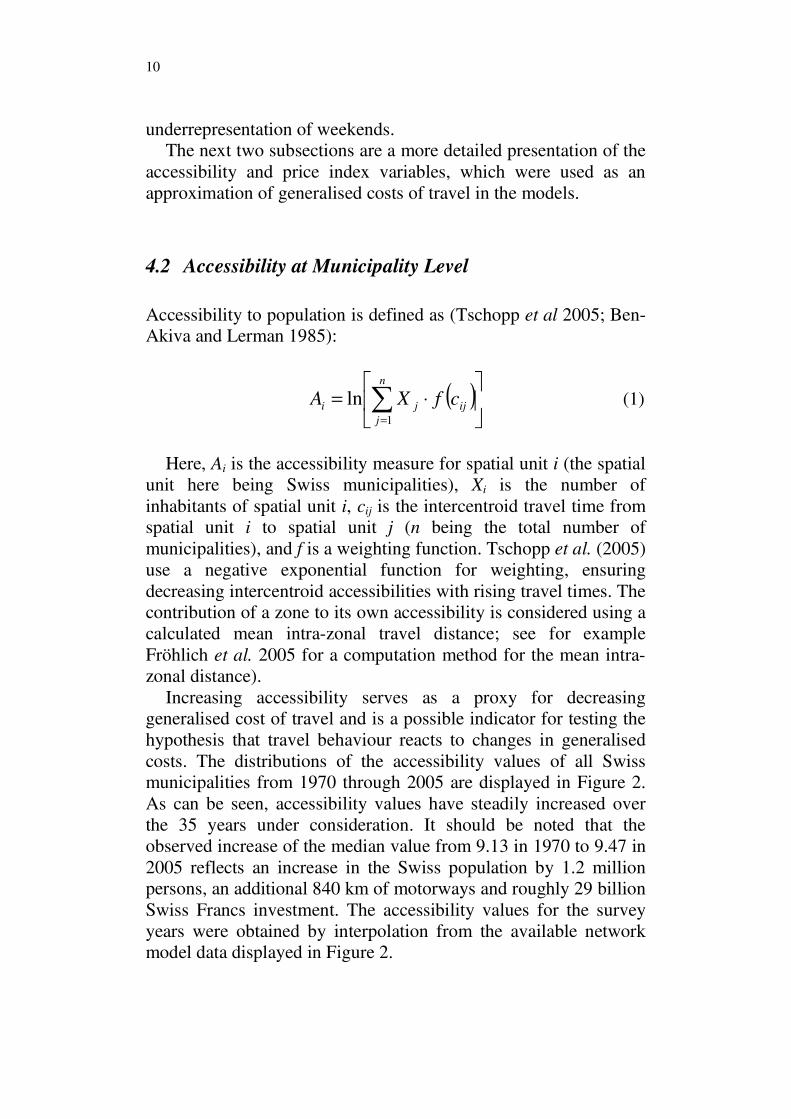
4.2 Accessibility at Municipality Level

Accessibility to population is defined as (Tschopp et al 2005; Ben-

Akiva and Lerman 1985):

( )

⋅= ∑

=

n

j

ijji cfXA1

ln (1)

Here, Ai is the accessibility measure for spatial unit i (the spatial

unit here being Swiss municipalities), Xi is the number of

inhabitants of spatial unit i, cij is the intercentroid travel time from

spatial unit i to spatial unit j (n being the total number of

municipalities), and f is a weighting function. Tschopp et al. (2005)

use a negative exponential function for weighting, ensuring

decreasing intercentroid accessibilities with rising travel times. The

contribution of a zone to its own accessibility is considered using a

calculated mean intra-zonal travel distance; see for example

Fröhlich et al. 2005 for a computation method for the mean intra-

zonal distance).

Increasing accessibility serves as a proxy for decreasing

generalised cost of travel and is a possible indicator for testing the

hypothesis that travel behaviour reacts to changes in generalised

costs. The distributions of the accessibility values of all Swiss

municipalities from 1970 through 2005 are displayed in Figure 2.

As can be seen, accessibility values have steadily increased over

the 35 years under consideration. It should be noted that the

observed increase of the median value from 9.13 in 1970 to 9.47 in

2005 reflects an increase in the Swiss population by 1.2 million

persons, an additional 840 km of motorways and roughly 29 billion

Swiss Francs investment. The accessibility values for the survey

years were obtained by interpolation from the available network

model data displayed in Figure 2.

11

Fig. 2 Distribution of accessibility values (on municipality level), 1970 – 2005

0.80

0.84

0.88

0.92

0.96

1.00

1970 1975 1980 1985 1990 1995 2000 2005

Year

Ind

ivid

ua

l tr

ave

l p

rice

in

de

x

Fig. 3 Evolution of inflation-adjusted individual travel price index, 1970 – 2005

4.3 Price Index for Individual Travel

The simple measure of accessibility as described above measures

generalised costs of travel as a function of travel time. In order to

have a monetary indicator in addition, price indices for individual

travel, as provided in Abay (2000) are used. The index, calculated

12

for years reaching back to 1972 is based on the Swiss national

consumer price index, and weighted to reflect inflation-adjusted

prices (the base year being 1972, hence the index is set to 1 for that

year). It represents a measure of transport prices relative to the

general consumer prices for all goods. Figure 3 shows the index’

evolution from 1972 through 2005.

5. Descriptive Analysis of the Pseudo Panel Dataset

This section deals with the characteristics of the pseudo panel

cohorts and their variation over time, and shows the generation and

life cycle effects of the representative indicators as well as the

above mentioned biases of the different survey methods.

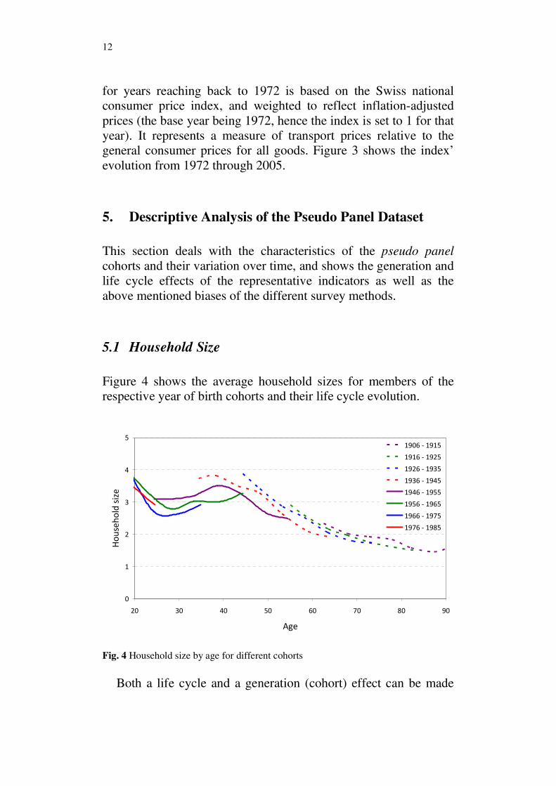
5.1 Household Size

Figure 4 shows the average household sizes for members of the

respective year of birth cohorts and their life cycle evolution.

0

1

2

3

4

5

20 30 40 50 60 70 80 90

Age

Ho

use

ho

ld s

ize

1906 - 1915

1916 - 1925

1926 - 1935

1936 - 1945

1946 - 1955

1956 - 1965

1966 - 1975

1976 - 1985

Fig. 4 Household size by age for different cohorts

Both a life cycle and a generation (cohort) effect can be made

13

out. The life cycle effect for all cohorts shows the expected trends.

Young adults tend to live in their parents’ homes and thus in large

households. As individuals approach their mid twenties, average

household size decreases as a consequence of moving out of the

family home and setting up their own households. Then, after

turning 30, the trend again turns to an increase in household size,

as the individuals settle down and have their own families. As the

mid 40’s pass, household sizes decrease again as an effect of

children moving out, and later on of spouses passing away. As for

the generation effect, it can be seen that younger cohorts tend to

live in smaller households. This can be explained by the larger

share of single person households (especially for young adults) as

well as by decreasing birth rates. Also, elderly people increasingly

tend to live on their own rather than moving back in with their

families or moving themselves to nursing homes.

5.2 Ownership of Car Driving License

The cohort and age effects for car driving license ownership are

displayed in Figure 5.

0.0

0.2

0.4

0.6

0.8

1.0

20 30 40 50 60 70 80 90

Age

Sh

are

of

car

dri

vin

g l

ice

nse

ow

ne

rs

1906 - 1915

1916 - 1925

1926 - 1935

1936 - 1945

1946 - 1955

1956 - 1965

1966 - 1975

1976 - 1985

Fig. 5 Car driving license ownership by age for different cohorts

The life cycle effects that are seen here are as expected. In fact,

14

young adults nowadays tend to acquire a driving license at quite

young age. In 2005, there is a practically constant, above 80 per

cent, share of car driving license owners throughout age groups, up

to the age of around 60. Car driving license ownership decreases

with age, and is much lower for cohorts born before the Second

World War, when licence holding was uncommon for women in

particular. Overall, the generation effect clearly tends towards

higher car driving license ownership in younger cohorts, again

pointing to an increased general availability of mobility tools over

time.

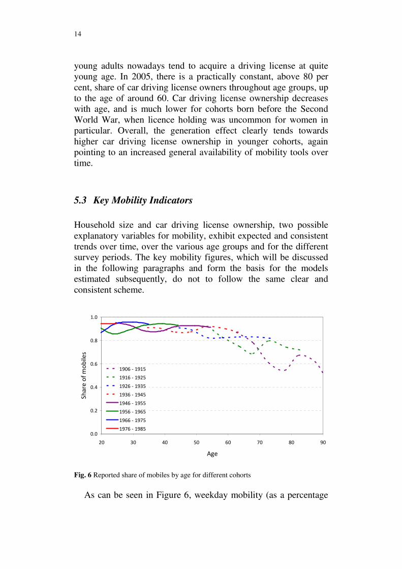
5.3 Key Mobility Indicators

Household size and car driving license ownership, two possible

explanatory variables for mobility, exhibit expected and consistent

trends over time, over the various age groups and for the different

survey periods. The key mobility figures, which will be discussed

in the following paragraphs and form the basis for the models

estimated subsequently, do not to follow the same clear and

consistent scheme.

0.0

0.2

0.4

0.6

0.8

1.0

20 30 40 50 60 70 80 90

Age

Sh

are

of

mo

bile

s

1906 - 1915

1916 - 1925

1926 - 1935

1936 - 1945

1946 - 1955

1956 - 1965

1966 - 1975

1976 - 1985

Fig. 6 Reported share of mobiles by age for different cohorts

As can be seen in Figure 6, weekday mobility (as a percentage

15

of individuals that reported at least one trip or out-of-home

activity) approximately reproduces the life cycle effect that one

would expect, that is continuously decreasing mobility with

increasing age. However, for each cohort, there is a slight drop in

reported mobility around the middle of the curve. These decreases

coincide with the 1984 and 1989 surveys. No natural reason for

this fluctuation being apparent, this suggests measurement errors

present in these years.

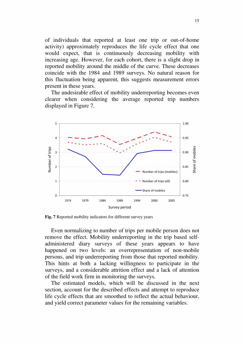
The undesirable effect of mobility underreporting becomes even

clearer when considering the average reported trip numbers

displayed in Figure 7.

0

1

2

3

4

5

1974 1979 1984 1989 1994 2000 2005

Survey period

Nu

mb

er

of

trip

s

0.75

0.80

0.85

0.90

0.95

1.00

Sh

are

of

mo

bil

es

Number of trips (mobiles)

Number of trips (all)

Share of mobiles

Fig. 7 Reported mobility indicators for different survey years

Even normalizing to number of trips per mobile person does not

remove the effect. Mobility underreporting in the trip based self-

administered diary surveys of these years appears to have

happened on two levels: an overrepresentation of non-mobile

persons, and trip underreporting from those that reported mobility.

This hints at both a lacking willingness to participate in the

surveys, and a considerable attrition effect and a lack of attention

of the field work firm in monitoring the surveys.

The estimated models, which will be discussed in the next

section, account for the described effects and attempt to reproduce

life cycle effects that are smoothed to reflect the actual behaviour,

and yield correct parameter values for the remaining variables.

16

6. Formulation and Estimation of the Structural

Equations Model

This section describes the model for the various mobility

indicators based on the factors listed above: share of mobiles,

number of journeys, number of trips, duration of out-of-home

activities, trip duration and estimated distances travelled.

The structural equations method (Bollen 1989) has seen wide

application in the travel behaviour research field (see Golob 2003

for a description of its benefits to travel behaviour research).

Applications include Lu and Pas (1999), an analysis of activity

participation and travel behaviour as a function of individuals’

sociodemographic attributes; Kuppam and Pendyala (2001), a

study of the relationships between commuters’ activity

participation, travel behaviour and trip chaining patterns; Simma

and Axhausen (2004), who analyse the interactions of travel

behaviour, accessibility and spatial characteristics in Upper Austria

based on a cross sectional dataset; as well as de Abreu e Silva and

Goulias (2009), where the influence of land use patterns on adult

workers’ travel behaviour is analysed.

The final structural equations model (SEM) was based upon

basic linear-in-parameters regression models (general linear

models, or GLM). The formulation and estimation of these models

yielded the expected effects of the independent variables on the

various mobility indicators (Weis 2008). The SEM is a

combination of the basic models in a unified framework. It models

the effects of the independent (exogenous) variables on all the

indicators (endogenous variables) simultaneously. Furthermore, the

model structure allows accounting for the reciprocal influences of

the endogenous variables on one another. It is a confirmatory

method for testing and quantifying assumed causal relationships

between various factors. The general formulation of the SEM is as

follows:

ζ+Γ+Β= xyy (2)

Here, y is an m x 1 vector of endogenous variables, Β an m x m

matrix of coefficients associated with the right-hand-side

endogenous variables, x an n x 1 vector of exogenous variables, Γ

an m x n matrix of coefficients associated with the exogenous

17

variables, and ξ an m x 1 vector of error terms associated with the

endogenous variables.

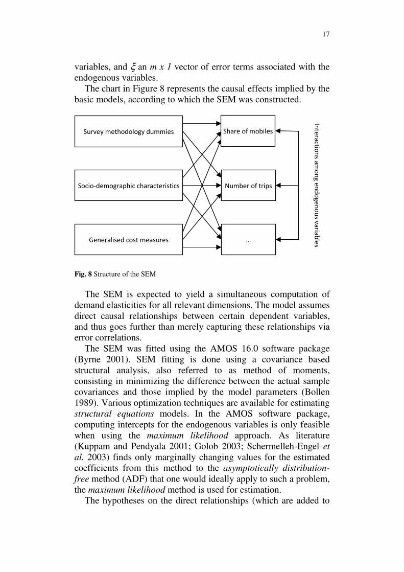
The chart in Figure 8 represents the causal effects implied by the

basic models, according to which the SEM was constructed.

Fig. 8 Structure of the SEM

The SEM is expected to yield a simultaneous computation of

demand elasticities for all relevant dimensions. The model assumes

direct causal relationships between certain dependent variables,

and thus goes further than merely capturing these relationships via

error correlations.

The SEM was fitted using the AMOS 16.0 software package

(Byrne 2001). SEM fitting is done using a covariance based

structural analysis, also referred to as method of moments,

consisting in minimizing the difference between the actual sample

covariances and those implied by the model parameters (Bollen

1989). Various optimization techniques are available for estimating

structural equations models. In the AMOS software package,

computing intercepts for the endogenous variables is only feasible

when using the maximum likelihood approach. As literature

(Kuppam and Pendyala 2001; Golob 2003; Schermelleh-Engel et

al. 2003) finds only marginally changing values for the estimated

coefficients from this method to the asymptotically distribution-

free method (ADF) that one would ideally apply to such a problem,

the maximum likelihood method is used for estimation.

The hypotheses on the direct relationships (which are added to

Survey methodology dummies

Socio-demographic characteristics

Generalised cost measures

Number of trips

…

Inte

ractio

ns a

mo

ng

en

do

ge

no

us v

aria

ble

s

Share of mobiles

18

the effects of the structural and socioeconomic variables described

above) between the cohort-level endogenous variables are as

follows:

• Increased weekday mobility will increase the number of

conducted trips. This conclusion is quite straightforward.

• Increased mobility, respectively the increased trip numbers it

brings about, will increase out-of-home-durations as well as

distances travelled.

• As a corollary, the number of trips per tour will increase under

the assumption that the number of tours remains roughly the

same (i.e., the additional trips are integrated into existing chains

rather than generating new journeys); or decrease if the reduced

generalised costs lead to more returns to the home location in

between out-of-home activities.

• As trip chains become longer, the effect on travelled distances

described above should be attenuated, as adding new trips to a

chain likely produces less mileage than conducting an entirely

new journey (as the return home trip is left out).

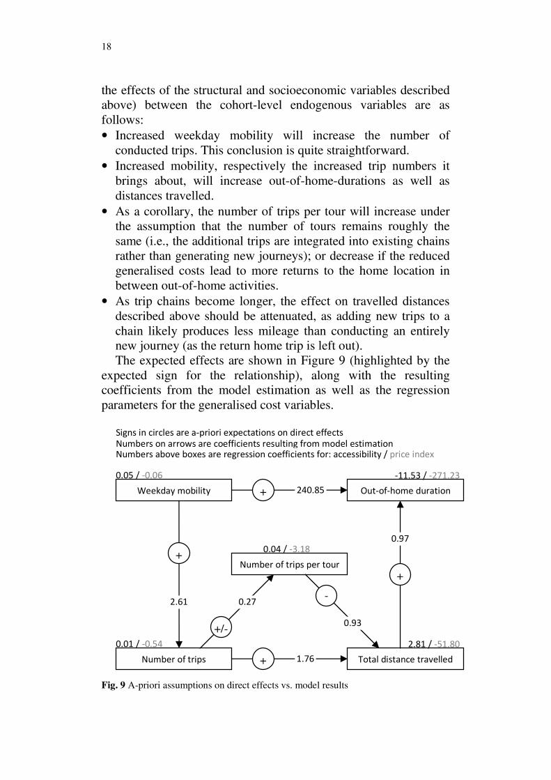
The expected effects are shown in Figure 9 (highlighted by the

expected sign for the relationship), along with the resulting

coefficients from the model estimation as well as the regression

parameters for the generalised cost variables.

Fig. 9 A-priori assumptions on direct effects vs. model results

Weekday mobility Out-of-home duration

Number of trips

Number of trips per tour

Total distance travelled

Numbers on arrows are coefficients resulting from model estimation Numbers above boxes are regression coefficients for: accessibility / price index

0.05 / -0.06 -11.53 / -271.23

0.01 / -0.54 2.81 / -51.80

0.04 / -3.18

+/-

+

+

+

+

- 2.61

240.85

1.76

0.97

0.93

0.27

Signs in circles are a-priori expectations on direct effects

19

All hypothesised effects except those on trip distance are

significant at the 5 per cent level and have the expected sign (see

above). The effect of trip chain complexity on travelled distance is

contrary to the assumptions postulated in the last section. Thus, the

addition of trips to existing chains appears to accentuate the

increase of covered distances induced by the higher general

mobility, instead of attenuating it by suppressing the return home

trips.

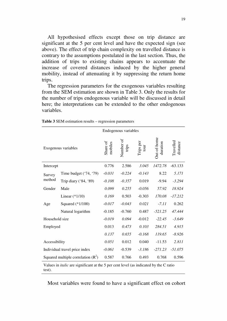
The regression parameters for the exogenous variables resulting

from the SEM estimation are shown in Table 3. Only the results for

the number of trips endogenous variable will be discussed in detail

here; the interpretations can be extended to the other endogenous

variables.

Table 3 SEM estimation results – regression parameters

Endogenous variables

Exogenous variables

Shar

e o

f

mo

bil

es

Nu

mb

er o

f

trip

s

Tri

ps

per

tour

Ou

t-o

f-ho

me

dura

tion

Tra

vell

ed

dis

tan

ce

Intercept 0.776 2.586 3.045 1472.78 -63.133

Time budget (‘74, ‘79) -0.031 -0.224 -0.143 8.22 5.171 Survey

method Trip diary (‘84, ‘89) -0.108 -0.357 0.019 -9.94 -3.294

Gender Male 0.099 0.255 -0.056 57.92 18.924

Linear (*1/10) 0.169 0.503 -0.303 170.08 -17.212

Squared (*1/100) -0.017 -0.043 0.021 -7.11 0.262 Age

Natural logarithm -0.185 -0.760 0.487 -521.25 47.444

Household size -0.019 0.094 -0.012 -22.45 -3.649

Employed 0.013 0.473 0.103 284.51 4.915

0.137 0.655 -0.168 119.65 -8.926

Accessibility 0.051 0.012 0.040 -11.53 2.811

Individual travel price index -0.061 -0.539 -3.186 -271.23 -51.075

Squared multiple correlation (R2) 0.587 0.766 0.493 0.768 0.596

Values in italic are significant at the 5 per cent level (as indicated by the C ratio

test).

Most variables were found to have a significant effect on cohort

20

level trip generation. The estimated fixed effects for the survey

methodologies confirm their above mentioned impact on the

dependent variable. The most significant negative effect on trip

reporting results for the trip based diary surveys in the 1980’s,

which confirms the conclusion drawn from Figure 7.

Males throughout generations are slightly more mobile than

females. The same holds for employed individuals as well as for

car driving license owners, the latter being an indication of a direct

effect of mobility tool ownership on reported mobility. Household

size has a slight negative effect on the dependent variable, thus

individuals from family households tend to be slightly less mobile

than those from single households.

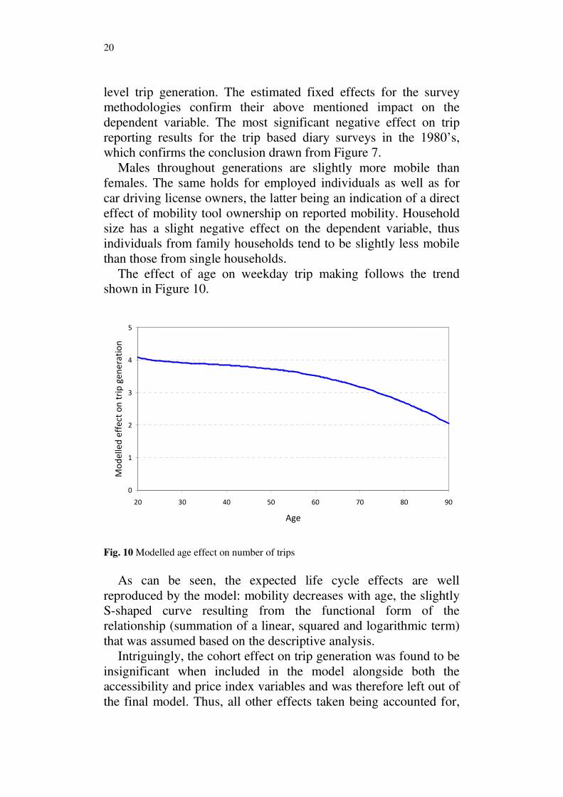
The effect of age on weekday trip making follows the trend

shown in Figure 10.

0

1

2

3

4

5

20 30 40 50 60 70 80 90

Age

Mo

de

lle

d e

ffe

ct o

n t

rip

ge

ne

rati

on

Fig. 10 Modelled age effect on number of trips

As can be seen, the expected life cycle effects are well

reproduced by the model: mobility decreases with age, the slightly

S-shaped curve resulting from the functional form of the

relationship (summation of a linear, squared and logarithmic term)

that was assumed based on the descriptive analysis.

Intriguingly, the cohort effect on trip generation was found to be

insignificant when included in the model alongside both the

accessibility and price index variables and was therefore left out of

the final model. Thus, all other effects taken being accounted for,

21

behaviour does not seem to vary much between birth year cohorts.

The life cycle effect is clearly dominant over the generation effect.

This absence of a generation effect is rather surprising given the

wide literature on long term effects of the improved childhood

nutrition of the post-war generations (for example Fogel 2004).

The most interesting effect is observed for the generalised cost

measures. In fact, all other influence factors being accounted for,

accessibility (here computed as the sum of the road and public

transport accessibilities) to population has a significant positive

effect on mobility. The inverse holds for the price index variable:

the negative effect implies that higher transport price levels cause

lower mobility and vice-versa. These findings suggest that

reductions in generalised costs do indeed increase travel demand.

The same conclusions hold for the other mobility indicators.

Accessibility has a significant positive influence, travel price a

negative one on all endogenous variables. The only endogenous

variable for which this does not hold is total out-of-home duration.

However, as this variable is part of a succession of reciprocal

effects between the other endogenous variables (see Figure 9), all

influenced positively by the accessibility variable, the total effect

of increasing accessibility on out-of-home duration is positive in

turn, as shown in the next section.

As far as trip chaining, defined here as the average number of

trips in a home-to-home tour, is concerned, the model shows that,

with decreasing generalised travel costs, the propensity to chain

trips seems to increase, as contrary to the postulated effect of the

cheaper home trip between two activities. Thus, additional trips are

integrated into existing chains rather than generating new tours. An

argument for this observation is that the increased distances (see

below) place the travellers at locations from which a return home is

not reasonably possible anymore.

The relative valuations for the generalised cost variables in the

various sub-models, as well as the total effects induced by the

generalised costs and the interrelations between the endogenous

variables, will be discussed in the next section.

7. Demand elasticities

Elasticities for the various demand variables are better suited for

22

the assessment of effects than the consideration of raw parameter

values. The values are computed at the sample means for all

variables and reflect the estimated effect of a 1 per cent increase in

accessibility, respectively price index, on the endogenous

variables. The results shown in Table 4 for the SEM include both

the effects of accessibility and price index on all dependent

variables and the direct influences of the endogenous variables on

one another, resulting from the coefficients shown in Figure 9.

Table 4 Accessibility and price index elasticities for GLM and SEM models

Demand elasticity Value

Weekday mobility 0.61

Number of trips 0.44

Number of trips per home-to-home tour 0.24

Total out-of-home duration 0.10

Accessbility

Total trip distance 1.14

Weekday mobility -0.06

Number of trips -0.19

Number of trips per home-to-home tour -1.66

Total out-of-home duration -0.84

Price index

Total trip distance -1.95

The values imply that, as a consequence of accessibility

increasing by 1 per cent:

• the share of mobiles increase by 0.6 per cent;

• 0.4 per cent more trips will be carried out;

• the number of trips per journey will increase by 0.2 per cent,

thus people will form slightly more complex trip chains;

• travelled distances will increase by 1.1 per cent.

The very high elasticities for travelled distances are rather

surprising at first sight, as they imply that a one per cent increase in

accessibility will generate roughly the equivalent relative increase

in daily mileage. The historical data confirm this trend though

(mileage increased substantially over time, from 26 kilometres per

day in 1974 up to 40 in 2005). Thus, as a result of a 10 per cent

increase in accessibility, the daily distance travelled by an average

individual would increase by roughly 4 kilometres (that is, from 40

to 44 kilometres per day).

23

The findings suggest a substantial influence of changed

generalised costs of travel (as implied by the rising accessibility

and decreasing price index) on individual mobility and trip

generation. Thus, accounting for relevant socioeconomic

influences, an induced travel effect for demand generation of

substantial size has been found.

However, the investment needed to increase it by about 3%

since 1970 should be kept in mind when conducting such thought

experiments. Further investigations on the necessary efforts to

bring about substantial accessibility increases are discussed in the

following section.

8. Interpretation of the results

The efforts that would be necessary to bring about massive

accessibility increases from the already high current levels were

assessed by the means of fictive scenarios. It was expected that

even large projects would induce only slight effects on global

accessibility values and thus the induced effects on travelled

distances should remain minor. The scenarios that were evaluated

(using the Swiss road network model) include:

• a global reduction of all travel times by 10, respectively 25, per

cent (with no new traffic assignment step);

• a capacity increase of one additional lane on all national roads,

respectively on all roads in the canton of Zurich (and the

subsequent computation of resulting travel times by a new

traffic assignment step);

• an increase of maximum speeds on all national roads by 10

kilometres per hour, respectively on all roads in the network

model by 10 kilometres per hour (and the subsequent

computation of resulting travel times by a new traffic

assignment step).

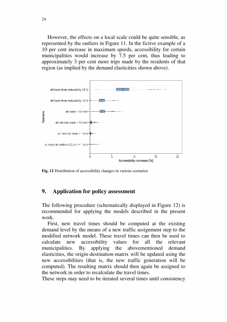
The population weighted distribution of the accessibility

increases induced by these scenarios is shown in Figure 11. Even

the dramatic investments needed to bring about capacity increases

as drastic as implied by the scenarios would lead to under-

proportional accessibility increases and thus have little impact on

induced traffic on an aggregate scale.

24

However, the effects on a local scale could be quite sensible, as

represented by the outliers in Figure 11. In the fictive example of a

10 per cent increase in maximum speeds, accessibility for certain

municipalities would increase by 7.5 per cent, thus leading to

approximately 3 per cent more trips made by the residents of that

region (as implied by the demand elasticities shown above).

Fig. 11 Distribution of accessibility changes in various scenarios

9. Application for policy assessment

The following procedure (schematically displayed in Figure 12) is

recommended for applying the models described in the present

work.

First, new travel times should be computed at the existing

demand level by the means of a new traffic assignment step to the

modified network model. These travel times can then be used to

calculate new accessibility values for all the relevant

municipalities. By applying the abovementioned demand

elasticities, the origin-destination-matrix will be updated using the

new accessibilities (that is, the new traffic generation will be

computed). The resulting matrix should then again be assigned to

the network in order to recalculate the travel times.

These steps may need to be iterated several times until consistency

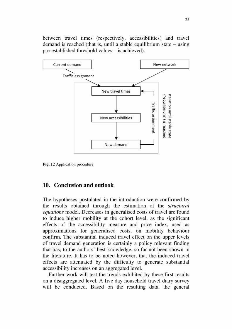
25

between travel times (respectively, accessibilities) and travel

demand is reached (that is, until a stable equilibrium state – using

pre-established threshold values – is achieved).

Fig. 12 Application procedure

10. Conclusion and outlook

The hypotheses postulated in the introduction were confirmed by

the results obtained through the estimation of the structural

equations model. Decreases in generalised costs of travel are found

to induce higher mobility at the cohort level, as the significant

effects of the accessibility measure and price index, used as

approximations for generalised costs, on mobility behaviour

confirm. The substantial induced travel effect on the upper levels

of travel demand generation is certainly a policy relevant finding

that has, to the authors’ best knowledge, so far not been shown in

the literature. It has to be noted however, that the induced travel

effects are attenuated by the difficulty to generate substantial

accessibility increases on an aggregated level.

Further work will test the trends exhibited by these first results

on a disaggregated level. A five day household travel diary survey

will be conducted. Based on the resulting data, the general

Current demand

New travel times

New accessibilities

Tra

ffic assig

nm

en

t

Itera

tion

un

til stab

le sta

te

(“eq

uilib

rium

”) is rea

che

d

Traffic assignment

New network

New demand

26

conditions for a given day of the household will be altered, thus

leading to changes in generalised costs for the planned activity

schedule. The household will then be asked to adapt their schedule

to the hypothetical situation by the means of an interactive

software tool.

It is hoped that this experiment will lead to further estimates of

the elasticities of the relevant travel demand dimensions and help

to validate the results that were obtained on the aggregate scale.

The results will help to improve the modelling of demand induced

by changing the generalised costs in agent-based travel demand

micro-simulations, such as MATSim (Balmer 2008), which will

also be used for the validation and an application of the obtained

results, especially as far as feedbacks from the transport system

(again modifying the generalised costs) are concerned.

Acknowledgments The authors gratefully acknowledge the financial support of the

SBT-Fonds administered by the Swiss Association of Transport Engineers (SVI

2004/012) and the advice of the steering committee chaired by Michel Simon, also

including Helmut Honermann, René Zbinden, Samuel Waldvogel and Stefan Dasen.

References

Abay, G. (2000). Die Preisentwicklung im Personenverkehr 1994-1999. Bern: Swiss

Federal Office for Spatial Development.

Aliesch, B., Sauter, J., Kuster, J. (2006). Räumliche Auswirkungen des Vereinatunnels:

Eine ex-post Analyse. Bern: Swiss Federal Office for Spatial Development.

Axhausen, K.W. (2008). Definition of movement and activity for transport modelling.

In: D.A. Hensher & K.J. Button (Eds.), Handbook of Transport Modelling, 2nd

edition (pp. 329-344).Oxford: Elsevier.

Balmer, M., Meister, K., Rieser, M., Nagel, K. Axhausen, K.W. (2008). Agent-based

simulation of travel demand: Structure and computational performance of

MATSim-T. Presented at the 2nd

TRB Conference on Innovations in Travel

Modeling, Portland, June 2008.

Barr, L.C. (2000). Testing for the significance of induced highway travel demand in

Metropolitan Areas. Transportation Research Record, 1706, 1-8.

Ben-Akiva, M.E., Lerman, S.R. (1985). Discrete Choice Analysis: Theory and

Application in Travel Demand. Cambridge: MIT Press.

Boarnet, M.G. & Crane, R. (2004). Travel by Design. The influence of urban form on

travel. Amsterdam: Springer.

Bodenmann, B.R. (2007). Modelle zur Standortwahl von Unternehmen. In T. Bieger,

C. Lässer, R. Maggi (Eds.) Jahrbuch 2006/2007 Schweizerische

Verkehrswirtschaft. St. Gallen: SVWG.

Bollen, K.A. (1989). Structural equations with latent variables. New York: John Wiley

& Sons, Inc.

Bush, S. B. (2003). Forecasting 65+ travel: An integration of cohort analysis and

travel demand modelling. Dissertation. Cambrdidge: Massachusetts Institute of

Technology.

Byrne, B. (2001). Structural equation modelling with AMOS – Basic concepts,

applications, and programming. East Sussex: Psychology Press.

27

Cairns, S., Hass-Klau, C., Goodwin, P.B. (1998). Traffic impact of highway capacity

reductions: Assessment of the evidence. London: ERSC Transport Studies Unit,

UCL.

Cervero, R. & Hansen, M. (2002). Induced travel demand and induced road

investment: A simultaneous equation analysis. Journal of Transport Economics and

Policy, 36 (3) 469-490.

Cerwenka, P. & Hauger, G. (1996). Neuverkehr – Realität oder Phantom?. Zeitschrift

für Verkehrswissenschaft, 67 (4) 286-326.

Dargay, J.M. (2002). Determinants of car ownership in rural and urban areas: A

pseudo-panel analysis. Transportation Research E, 38 (5) 351-366.

Dargay, J.M. (2007). The effect of prices and income on car travel in the UK.

Transportation Research A, 41 (10) 949-960.

Deaton, A. (1985). Panel data from time series of cross sections. Journal of

Econometrics, 30 (1) 109-126.

De Abreu e Silva, J. & Goulias, K.G. (2009). Using structural equations modelling to

unravel the influence of land use patterns on travel behavior of urban adult workers

of Puget Sound region. Presented at the 88th Annual Meeting of the Transportation

Research Board, Washington, D.C., January 2009.

De Corla-Souza, P. & Cohen, H. (1999). Estimating induced travel for evaluation of

metropolitan highway expansion. Transportation, 26 (3) 249-262.

Eurostat (2008). Nomenclature of territorial units for statistics – NUTS statistical

regions of Europe. Eurostat.

http://ec.europa.eu/eurostat/ramon/nuts/home_regions_en.html. Accessed 22

October 2009.

Fogel, R.W. (2004). The escape from hunger and premature death, 1700-2100,

Europe, America and the Third World. Cambridge:Cambridge University Press.

Fröhlich, P. (2003). Induced traffic: Review of the explanatory models. Presented at

the 3rd Swiss Transport Research Conference, Ascona, March 2003.

Fröhlich, P. (2008). Travel behavior changes of commuters from 1970-2000.

Transportation Research Record, 2082, 35-42.

Fröhlich, P., Tschopp, M., Axhausen, K.W. (2005). Netzmodelle und Erreichbarkeit in

der Schweiz: 1950-2000. In K.W. Axhausen & L. Hurni (Eds.) Zeitkarten Schweiz

1950-2000 (ch. 2). Zurich: IVT and IKA, ETH Zurich.

Fulton, L.M., Noland, R.B. Meszler, D.J., Thomas, J.V. (2000). A statistical analysis

of induced travel effects in the U.S. Mid-Atlantic Region. Journal of

Transportation and Statistics, 3 (1) 1-14.

Giacomazzi, F. Clerici, R. Marti, P. Rudel, R. Brugnoli, G., Passardi-Gianola, L.,

Gianola, G., Meneghin, F., von Wartburg, S. (2004). Räumliche Auswirkungen der

Verkehrsinfrastrukturen in der Magadinoebene: Eine ex-post Analyse. Bern: Swiss

Federal Office for Spatial Development.

Golob, T.F. (2003). Structural equation modeling for travel behavior research.

Transportation Research B, 37 (1) 1-25.

Goodwin, P.B. (1992). Review of new demand elasticities. Journal of Transport

Economics and Policy, 26 (2) 155-169.

Goodwin, P.B. (1996). Empirical evidence on induced traffic. Transportation, 23 (1)

35-54.

Goodwin, P.B., Dargay, J. Hanly, M. (2004). Elasticities of road traffic and fuel

consumption with respect to price and income: A review. Transport Reviews, 24 (3)

275-292.

Goulias K.G., Kilgren, N., Kim, T.-G. (2003). A decade of longitudinal travel behavior

observation in the Puget Sound region: Sample composition, summary statistics,

and a selection of first order findings. Presented at the 10th

International

28

Conference on Travel Behavior Research, Lucerne, August 2003.

Goulias K.G., Blain, L., Kilgren, N., Michalowski, T. Murakami, E. (2007). Catching

the next big wave: Are the observed behavioral dynamics of the Baby Boomers

forcing us to rethink regional travel demand models?. Transportation Research

Record, 2014, 67-75.

Graham, D.J. & Glaister, S. (2004). Road traffic demand elasticity estimates: A

review. Transport Reviews, 24 (3) 261-274.

Güller, P., Schenkel, W. De Tommasi, R. and Oetterli, D. (2004). Räumliche

Auswirkungen der Zürcher S-Bahn: Eine ex-post Analyse. Bern: Swiss Federal

Office for Spatial Development.

Huang, B. (2007). The use of pseudo panel data for forecasting car ownership.

Dissertation. London: University of London.

Jones, P.M., Dix, M., Clarke, M. Heggie, I. (1980) Understanding Travel Behaviour.

Aldershot: Gower.

Kitamura, R. (2000): Longitudinal methods. In D.A. Hensher & K.J. Button (Eds.)

Handbook of Transport Modelling (pp. 113-129). Oxford: Elsevier Science.

Kumar, A & Levinson, D. (1992). Specifying, estimating and validating a new trip

generation model: A case study of Montgomery County, Maryland. Transportation

Research Record, 1413, 107-113.

Kuppam, A.R. & Pendyala, R.M. (2001). A structural equations analysis of

commuters’ activity and travel patterns. Transportation, 28 (1) 33-54.

Lee, D.B., Klein, L.A., Camus, G. (1999). Induced traffic and induced demand.

Transportation Research Record, 1659, 68-75.

Lleras, G.C., Simma, A., Ben-Akiva, M. Schafer, A., Axhausen, K.W., Furutani, T.

(2003). Fundamental relationships specifying travel behavior – An international

travel survey comparison. Presented at the 82nd

Annual Meeting of the

Transportation Research Board, Washington, D.C., January 2003.

Lu, X. & Pas, E.I. (1999). Socio-demographics, activity participation and travel

behavior. Transportation Research A, 33 (1) 1-18.

Madre, J.-L., Axhausen, K.W., Brög, W. (2007). Immobility in travel diary surveys.

Transportation, 34 (1) 107-128.

Mason, W.M. & Wolfinger, N.H. (2004). Cohort analysis. In N.J. Smelser & P.B.

Baltes (Eds.) International Encyclopedia of Social and Behavioral Sciences (pp.

2189-2194). Amsterdam: Elsevier.

Meier, E. (1989). Neuverkehr infolge Ausbau und Veränderung des Verkehrssystems.

Dissertation. Zurich: IVT, ETH Zurich.

Mokhtarian, P.L. & Cao, X. (2008). Examining the impacts of residential self-selection

on travel behavior: A focus on methodologies. Transportation Research B, 42 (3)

204-228.

Mokhtarian, P.L. & Chen, C. (2004). TTB or not TTB, that is the question: A review

and analysis of the empirical literature on travel time (and money) budgets.

Transportation Research A, 38 (9) 643-675.

Noland, R.B. (2001). Relationships between highway capacity and induced vehicle

travel. Transportation Research A, 35 (1) 47-72.

Noland, R.B. & Cowart, W.A. (2000).Analysis of metropolitan highway capacity and

the growth in vehicle miles of travel. Transportation, 27 (4) 363-390.

Noland, R.B. & Lewison, L.L. (2000). Induced travel: A review of recent literature and

the implications for transportation and environmental policy. Presented at the

European Transport Conference, Cambridge, September 2000.

Oum T. (1989). Alternative demand models and their elasticity estimates. Journal of

Transport Economics and Policy, 23 (2) 163-187.

Ortúzar, J. de D. & Willumsen, L.G. (2001). Modelling transport. Chichester: Wiley.

29

Primerano, F., Taylor, M.A.P., Pitaksrigkarn, L., Tisato, P. (2008). Defining and

understanding trip chaining behaviour. Transportation, 35 (1) 55-72.

Schermelleh-Engel, K., Mossburger, H., Müller, H. (2003). Evaluating the fit of

structural equation models: Tests of significance and descriptive goodness-of-fit

measures. Methods of Psychological Research - Online, 8 (2) 23-74.

Simma, A. (2003). Geschichte des Schweizerischen Mikrozensus zum

Verkehrsverhalten. Presented at the 3rd

Swiss Transport Research Conference,

Ascona, March 2003.

Simma, A. & Axhausen, K.W. (2003). Interactions between travel behaviour,

accessibility and personal characteristics: The case of the Upper Austria region.

European Journal of Transport and Infrastructure Research, 3 (2) 179-198.

Tschopp, M. (2007). Erreichbarkeitsveränderungen und Raumstrukturelle

Entwicklung. Dissertation. Zurich: IVT, ETH Zurich.

Tschopp. M., Keller, P., Schiedt, H.U., Frei, T., Reubi, S., Axhausen, K.W. (2003).

Raumnutzung in der Schweiz: Eine Historische Raumstruktur-Datenbank.

Arbeitsberichte Verkehrs- und Raumplanung, 165. Zurich: IVT, ETH Zurich.

Tschopp, M., Fröhlich, P. Axhausen, K.W. (2005). Accessibility and spatial

development in Switzerland during the last 50 years. In D.M. Levinson & K.J.

Krizek (Eds.) Access to Destinations (pp. 361-376). Oxford: Elsevier.

Van Wee, B., Rietveld, P. Meurs, H. (2006). Is average daily travel time expenditure

constant? In search of explanations for an increase in average travel time. Journal

of Transport Geography, 14 (2)109-122.

Varian, H.R. (1992). Microeconomic Analysis. New York: WW Norton.

Weis, C. (2008). Modelling travel behaviour using pseudo panel data – first results.

Presented at the 8th

Swiss Transport Research Conference, Ascona, October 2008.

Weis, C. & Axhausen, K.W. (2009). Aktivitätenorientierte Analyse des Neuverkehrs –

Intermediate Report SVI 2005/203. Bern: Swiss Federal Roads Office.

Yee, J.L. & Niemeier, D.A. (2000). Analysis of activity duration using the Puget

Sound transportation panel. Transportation Research A, 34 (8) 607-624

Zumkeller, D., Chlond, B., Ottmann, P., Kagerbauer, M., Kuhnimhof, T. (2009).

Deutsches Mobilitätspanel (MOP) – WissenschaftlicheBegleitung und erste

Auswertungen. Karlsruhe: Institut für Verkehrswesen, Universität Karlsruhe.