Embed Size (px)
Citation preview

Research Collection
Doctoral Thesis
From theory to practiceFundamental properties and services of mobile ad hoc networks
Author(s): Stüdi, Patrick M.
Publication Date: 2008
Permanent Link: https://doi.org/10.3929/ethz-a-005713655
Rights / License: In Copyright - Non-Commercial Use Permitted
This page was generated automatically upon download from the ETH Zurich Research Collection. For moreinformation please consult the Terms of use.
ETH Library

DISS. ETH NO. 18078
From Theory to Practice:
Fundamental Properties and Services
of Mobile Ad Hoc Networks
A dissertation submitted to the
SWISS FEDERAL INSTITUTE OF TECHNOLOGY ZURICH
for the degree of
Doctor of Sciences
presented by
PATRICK STUEDI
Dipl. Inf.-Ing., ETH Zurich
born 25.07.1974
citizen of
Zurich ZH
accepted on the recommendation of
Prof. Dr. Gustavo Alonso, examiner
Prof. Dr. Timothy Roscoe, co-examiner
Prof. Dr. Roger Wattenhofer, co-examiner
Dr. Antony Rowstron, co-examiner
2008

Abstract
Mobile Ad Hoc Networks (MANETs) by definition operate without pre-establishedinfrastructure. On the one hand side, this can be seen as an advantage since it makesthem usable in situations where an infrastructure is not available, such as, e.g., insettings of emergency response. On the other hand, the lack of infrastructure posesdifficult challenges to protocol design and software architecture for such networks.One example is wireless media access. In contrast to traditional wireless networkswhere nodes communicate through base stations, there is no dedicated network com-ponent to control the media access of the nodes in MANETs. This makes schedulingwireless transmissions complicated and affects the overall throughput capacity of thenetwork. Another example are application level services. Many advanced applica-tions on MANETs require basic services such as, e.g., DNS, SIP and SLP to operate.These services, however, typically rely on centralized components for storing the re-quired networking information, components that are not available in MANETS. Inthis thesis, we study several problems occurring in MANETs at different places inthe network stack.
The first part studies fundamental properties of MANETs on the physical anddata link layer, such as, e.g., capacity, connectivity, quality of service, etc. Under-standing the behavior of those properties is important because they describe thelimitations applications face in MANETs. Fundamental properties like connectivityand capacity have been in the focus of research over the past years. The novelty ofthe work presented in this thesis is that we use a formal model approach combinedwith Monte-Carlo methods. The approach chosen has a two-fold advantage: it isprotocol independent and, at the same time, the computations are performed on anetwork model that is based on realistic physical properties. In the thesis we showhow such an approach can be used to study the complex interactions between dif-ferent interference and signal propagation models on the throughput capacity of anetwork.
The second part of the thesis studies ad hoc networks from a system perspec-tive. Thereby our goal is to provide a networking infrastructure that transparentlyhides the complexity of the underlying ad hoc network to upper layers. We believethat the ability to run traditional Internet-based applications in ad hoc networks isthe key for MANETs to become ubiquitous. This dissertation presents several net-work abstractions and services that support this goal. First, we present the designand implementation of a virtual network interface which allows to integrate nodesequipped with different media access technologies into one single IP based MANET.The virtual interface accounts for the fact that today’s devices become more and moreheterogeneous, particularly with respect to their wireless access technology. Second,we present the architecture of several fundamental networking services which allowInternet-based applications to run transparently in MANETs. Opening ad hoc net-works for Internet applications such as chat or VoIP is an important step towardsMANETs to be used in the everyday life. For each of the networking services, DNS,SIP and SLP, we show how they provide a smooth MANET-Internet phase transition.The core building block of those networking services is MAND, a distributed systemfor storing and searching key/value pairs. MAND is highly efficient as distribution

of both tuples and requests happens based on piggybacking onto routing messagesthat the MANET network uses anyway, thus causing no additional message traffic.The thesis evaluates MAND together with the services built on top. The evaluationis done on a 30 node testbed and on a deployment of 20 Nokia N800 handheld de-vices. As a last part of this thesis, we present a social networking application for adhoc networks. AdSocial allows users within a MANET to discover each other andbrowse through other people’s personal profile. AdSocial also integrates chat, VoIPand video. Similar to other networking services described in this thesis, AdSocial usesthe MAND system to advertise user information, thus not imposing any additionaltraffic load.

Zusammenfassung
Mobile Ad Hoc Netzwerke (MANETs) operieren per definition ohne eine bestehendeInfrastruktur. Dies kann zum einen als Vorteil angesehen werden da es erlaubt sol-che Netze in Situation einzusetzen wo keine Infrastruktur vorhanden ist, wie z.b inNotfall Szenarien. Zum anderen fuehrt das Fehlen einer Infrastruktur aber auch zuSchwierigkeiten bezueglich Protokoll Design und Software Architektur. Ein Beispielsind Medien Zugriffsverfahren. Im Unterschied zu traditionellen Funknetzen, wo dieKommunikation zwischen Geraeten (Knoten) ueber Basisstationen abgewickelt wird,gibt es in MANETs keine dedizierten Netzwerk Komponenten die den Zugriff aufdas Funk Medium kontrollieren. Dies erschwert die Koordination von Datenueber-tragungen zwischen verschiedenen Knoten erheblich und beeintraechtigt den Daten-durchsatz. Ein anderes Beispiel sind Applikationen und Services in MANETs. Vieleanspruchsvolle Applikationen basieren auf Services wie DNS (Domain Name Service),SIP (Session Initiation Protokoll) oder SLP (Service Location Protokoll). Diese Ser-vices wurden aber urspruenglich fuer das Internet entwickelt und erforden gewissezentrale Komponenten, welche in MANETs nicht verfuegbar sind. Diese Dissertationbefasst sich mit Problemen in MANETs auf verschiedensten Netzwerk Schichten.
Der erste Teil dieser Dissertation befasst sich mit fundamentalen Eigenschaftenim Bereich der physikalischen Schicht. Eigenschaften wie Netzwerk Zusammenhaen-gigkeit oder Netzwerk Durchsatz sind entscheidende Kriterien hinsichtlich der Fragewelche Klasse von Applikationen fuer MANETs ueberhaupt relevant sind. In denvergangenen Jahren rueckten fundamentale Eigenschaften wie ’Netzwerk Durchsatz’verstaerkt ins Blickfeld von Forschung. Die Neuartigkeit der durch diese Dissertationpraesentierten Arbeit liegt im verwendeten Ansatz, einer Kombination von formalenModellen mit Monte-Carlo Methoden. Dieser Ansatz hat zwei wesentliche Vorteile.Er ist unanbhaengig von konkreten Netzwerk Protokollen und gleichzeitig basierendie Berechnungen auf einem Netzwerk Modell mit realistischen physikalischen Eigen-schaften. Die vorliegenden Arbeit zeigt auf, wie ein solcher Ansatz verwendet werdenkann um komplexe Zusammenhaenge zwischen verschiedensten Inteferenz und Signal-ausbreitungs Modellen zu untersuchen.
Der zweite Teil dieser Dissertation studiert Ad Hoc Netzwerke von einer SystemPerspektive. Das verfolgte Ziel ist es, eine Netzwerk Infrastruktur zu entwickeln, wel-che die Komplexitaet des unterliegenden ad hoc Netzwerkes versteckt vor hoeherliegenden Services und Applikationen. Wir sind ueberzeugt, dass die Faehigkeit exi-stierende Netzwerk Applikationen ohne Veraenderung nahtlos in ad hoc Netzwerkenbetreiben zu koennen der Schluessel ist um ad hoc Netzwerke einer breiteren Massezugaenglich zu machen. Die vorliegende Doktorarbeit presentiert verschiedene Netz-werk Abstraktionen und Dienste welche diese Ueberlegung umsetzen. Zuerst stellt dieArbeit in virtuelles Netzwerk Interface vor welches es ermoeglicht Knoten mit ver-schiedensten Medienzugriffsverfahren in ein einheitliches IP basiertes ad hoc Netzwerkzu integrieren. Das virtuelle Interface koennte einen wichtigen Baustein in zukuenfti-gen heterogenen Netzwerken darstellen wo die einzelnen Geraete mit verschiedenstenFunk Technologien ausgeruested sind. Als naechstes presentiert die vorliegende Ar-beit die Software Architektur von verschiedensten fundamentalen Netzwerk Diensten

welche es ermoeglichen klassische Internet-basierte Applikation transparent und oh-ne Veraenderung in ad hoc Netzwerken zu betreiben. Die Moeglichkeit existierendeApplikationen wie Chat oder VoIP in ad hoc Netzwerken zu verwenden, spontan undohne jegliche System Aenderungen, stellt einen wichtigen Schritt dar hinsichtlich demGebrauch von Ad Hoc Netzen im taeglichen Leben von Nutzern. Fuer jeden in dieserArbeit presentierten Netzwerk Dienst, DNS, SLP, SIP, wird aufgezeigt inwiefern undfuer welche Art von Applikationen der Dienst einen nathlosen MANET/Internet Ue-bergang darstellt. Den wichtigsten Baustein im Design dieser Dienste stellt MANDdar, eine neuartige Infrastruktur zum verteilen, speichern und suchen von Schlues-sel/Wert Paaren (Tuples) in MANETs. MAND ist message effizient da Tuples einzigund allein per Huckepack angehaengt an bestehende Routing Packete im Netzwerkverteilt werden. In der Dissertation wird MAND zusammen mit den darauf aufbauen-den Services evaluirt. Die Evaluation findet auf einem Testbed von 30 Knoten und perSimulation statt. Zusaetzlich wurden alle in dieser Dissertation entwickelten Servicesund Applikation auf einem Netzwerk von 20 Nokia Handheld Geraeten eingesetzt.Im letzen Teil dieser Dissertation stellen wir eine neuartige Applikation fuer ’socialnetworking’ in ad hoc Netzwerken vor. AdSocial ermoeglich das gegenseitige Auffin-den von Nutzern mit aehnlichen Interessen in Ad Hoc Netzen und das durchsuchenvon persoenlichen Profilen. Zusatzlich integriert AdSocial verschiedenste Applikatio-nen wie Chat, VoIP oder Video. Ahenlich wie die vorgaengig persentierten NetzwerkDienste verwendet auch AdSocial das MAND System um Informationen der Nutzereffizient und ohne Packet overhead im Netzwerk verfuegbar zu machen.

Acknowledgements
First of all, I want to thank my advisor Gustavo Alonso for having given me thechance to pursue a PhD in his group. Through all the years of my studies, you alwayssupported me in following my own ideas for which I am very grateful. At the sametime, your advice to always question the practical relevance of my research helpedme to define the problem outline in the first place. It is the combination of the rightamount of freedom and the necessary guidance which I appreciate so much and whichenabled me to write this thesis. It was a pleasure to work with you!
I also would like to thank my co-examiners Timothy Roscoe, Roger Wattenhoferand Antony Rowstron for their willingness to read through my thesis and serve onmy committee board. It is an honor for me to have three such renowned researchers,for whose works I have the greatest respect, in my committee. Your comments andour discussions have been of a big help in improving the thesis as well as in shapingmy research skills.
Many thanks go to the members of the Systems group. I would like to thank ReneMueller, Mike Duller, Spyros Voulgaris and Bioern Bioernstad for all the lively andconstructive discussions we had; Thomas Heinis and Ionut Subasu, my office mates,for creating an inspiring working environment and for adding a pinch of humor to eachworking day. Oriana Riva for all the help with the wireless experiments. Workingwith real ad hoc network deployments can be difficult, but Oriana always served as adriving force. Urs Stettler & Emre Sarigol for their help dealing with the deploymenton the Nokia handheld devices. Simonetta Zysset and Eva Ruiz for always providing afriendly environment and for assisting with organizing trips and proofreading papers.
A special thank you goes to my family who supported me in many ways. Christian,my brother, for challenging me in tennis and keeping my physical and mental fitnessbalanced. Finally, my deepest thanks belong to Martina. I am deeply indebted toher for all the patience she exercised during many work intensive days and weeks.Her love was my main source of motivation throughout this thesis.

Contents
1 Introduction: From Theory to Practice 13
I Fundamental Properties 17
2 Fundamental Properties of Ad Hoc Networks 19
2.1 Overview . . . . . . . . . . . . . . . . . . . . . . . . . . . . . . . . . . 19
2.2 Approach . . . . . . . . . . . . . . . . . . . . . . . . . . . . . . . . . 20
2.3 Related Work . . . . . . . . . . . . . . . . . . . . . . . . . . . . . . . 21
3 Model and Computation Method 27
3.1 Network Model . . . . . . . . . . . . . . . . . . . . . . . . . . . . . . 27
3.2 Monte-Carlo Method . . . . . . . . . . . . . . . . . . . . . . . . . . . 28
4 Connectivity 31
4.1 Constant Transmission Power . . . . . . . . . . . . . . . . . . . . . . 31
4.2 Adaptive Transmission Power . . . . . . . . . . . . . . . . . . . . . . 35
4.3 Summary . . . . . . . . . . . . . . . . . . . . . . . . . . . . . . . . . 37
5 Capacity: Model 39
5.1 Overview . . . . . . . . . . . . . . . . . . . . . . . . . . . . . . . . . . 39
5.2 Node Relationships . . . . . . . . . . . . . . . . . . . . . . . . . . . . 41
5.3 Scheduling Algorithms . . . . . . . . . . . . . . . . . . . . . . . . . . 42
5.4 Schedule Graph . . . . . . . . . . . . . . . . . . . . . . . . . . . . . . 45
5.5 Throughput Capacity . . . . . . . . . . . . . . . . . . . . . . . . . . . 46
5.6 Summary . . . . . . . . . . . . . . . . . . . . . . . . . . . . . . . . . 47
6 Capacity: Validation 49
6.1 Capacity of static networks . . . . . . . . . . . . . . . . . . . . . . . . 49
6.2 Capacity of larger networks . . . . . . . . . . . . . . . . . . . . . . . 51
7 Continuing Experiments 57
7.1 Network settings . . . . . . . . . . . . . . . . . . . . . . . . . . . . . 57
7.2 Capacity under different interference models . . . . . . . . . . . . . . 58
7.3 Effects of log-normal shadowing . . . . . . . . . . . . . . . . . . . . . 60
7.4 Adaptive Power Assignment . . . . . . . . . . . . . . . . . . . . . . . 62
7.5 Summary . . . . . . . . . . . . . . . . . . . . . . . . . . . . . . . . . 63
8 Distributed Bandwidth Reservation 65
8.1 Problem Statement . . . . . . . . . . . . . . . . . . . . . . . . . . . . 66
8.2 Reservation Recall and Precision . . . . . . . . . . . . . . . . . . . . 67
8.3 Precision and Recall in Random Networks . . . . . . . . . . . . . . . 68
8.4 End-to-end reservations . . . . . . . . . . . . . . . . . . . . . . . . . . 71
8.5 Reservation quality and Loss in random networks . . . . . . . . . . . 72
8.6 Summary . . . . . . . . . . . . . . . . . . . . . . . . . . . . . . . . . 73
II System 75
9 The invisible ad hoc network 77
10 Heterogeneous Mobile Ad Hoc Networks 79
10.1 PolyMAC in MANETs using Bluetooth and 802.11 . . . . . . . . . . 80
10.2 Overview . . . . . . . . . . . . . . . . . . . . . . . . . . . . . . . . . . 81
10.3 A MAC Layer Approach . . . . . . . . . . . . . . . . . . . . . . . . . 82
10.4 System Evaluation . . . . . . . . . . . . . . . . . . . . . . . . . . . . 88
10.5 Discussion . . . . . . . . . . . . . . . . . . . . . . . . . . . . . . . . . 91
10.6 Related Work . . . . . . . . . . . . . . . . . . . . . . . . . . . . . . . 92
10.7 Summary . . . . . . . . . . . . . . . . . . . . . . . . . . . . . . . . . 93
11 MAND: Mobile Ad Hoc Network Directory 95
11.1 Problem Statement . . . . . . . . . . . . . . . . . . . . . . . . . . . . 95
11.2 System Model . . . . . . . . . . . . . . . . . . . . . . . . . . . . . . . 97
11.3 Routing handler . . . . . . . . . . . . . . . . . . . . . . . . . . . . . . 101
11.4 Interface Semantics . . . . . . . . . . . . . . . . . . . . . . . . . . . . 103
11.5 Evaluation . . . . . . . . . . . . . . . . . . . . . . . . . . . . . . . . . 106
11.6 Simulation . . . . . . . . . . . . . . . . . . . . . . . . . . . . . . . . . 110
11.7 Related Work . . . . . . . . . . . . . . . . . . . . . . . . . . . . . . . 113
11.8 Summary . . . . . . . . . . . . . . . . . . . . . . . . . . . . . . . . . 114
12 Service Discovery and MANET-Internet Integration 117
12.1 The Service Location Protocol (SLP) . . . . . . . . . . . . . . . . . . 118
12.2 MANET-SLP . . . . . . . . . . . . . . . . . . . . . . . . . . . . . . . 119
12.3 MANET-Internet integration . . . . . . . . . . . . . . . . . . . . . . . 120
12.4 Performance . . . . . . . . . . . . . . . . . . . . . . . . . . . . . . . . 122
12.5 Related Work . . . . . . . . . . . . . . . . . . . . . . . . . . . . . . . 123
12.6 Summary . . . . . . . . . . . . . . . . . . . . . . . . . . . . . . . . . 124
13 DOPS: Domain Name and Presence Service 125
13.1 Standard DNS . . . . . . . . . . . . . . . . . . . . . . . . . . . . . . . 125
13.2 DOPS in the MANET . . . . . . . . . . . . . . . . . . . . . . . . . . 125
13.3 Seamless integration with the Internet . . . . . . . . . . . . . . . . . 127
13.4 Performance . . . . . . . . . . . . . . . . . . . . . . . . . . . . . . . . 129
13.5 Related Work . . . . . . . . . . . . . . . . . . . . . . . . . . . . . . . 133
13.6 Summary . . . . . . . . . . . . . . . . . . . . . . . . . . . . . . . . . 134
14 SIPHoc: Distributed Session Initiation in MANETs 13514.1 SIP Overview . . . . . . . . . . . . . . . . . . . . . . . . . . . . . . . 13514.2 SIPHoc in MANETs . . . . . . . . . . . . . . . . . . . . . . . . . . . 13614.3 Internet-connected MANETs . . . . . . . . . . . . . . . . . . . . . . . 13814.4 Case Study: VoIP in MANETs . . . . . . . . . . . . . . . . . . . . . 13914.5 Related Work . . . . . . . . . . . . . . . . . . . . . . . . . . . . . . . 14314.6 Summary . . . . . . . . . . . . . . . . . . . . . . . . . . . . . . . . . 144
15 Network services in MANETs: A Discussion 145
16 Social Ad Hoc Networking 14916.1 Overview . . . . . . . . . . . . . . . . . . . . . . . . . . . . . . . . . . 14916.2 Architecture . . . . . . . . . . . . . . . . . . . . . . . . . . . . . . . . 14916.3 Deployment . . . . . . . . . . . . . . . . . . . . . . . . . . . . . . . . 15116.4 Measurements . . . . . . . . . . . . . . . . . . . . . . . . . . . . . . . 15216.5 Summary . . . . . . . . . . . . . . . . . . . . . . . . . . . . . . . . . 156
17 Conclusion 157

12

Chapter 1
Introduction:From Theory to Practice
Mobile Ad Hoc Networks (MANETs) combine various extreme aspects of todayscomputer networks. Communication in the network is wireless. Packets may traversemultiple wireless devices (nodes) towards their destination. The network operateswithout any pre-existing infrastructure. The nodes in the network are mobile. Thedevices may have only limited resources.
The combination of those network aspects is unique. There are other forms ofwireless networks such as Wireless LANs, but they use a pre-existing infrastructureof base-stations for communication. There are infrastructure-less networks, such asSensor Networks, but there nodes typically are not mobile. Mobility is supportedby cellular networks, such as, e.g., GSM or UMTS. But again, those networks arebased on a stationary infrastructure which is not only composed of access points, butalso of centralized location servers to determine the position of the devices. Thereare network forms, such as traditional Peer-to-peer networks, which operate withoutcentralized software components, but those systems rely on the Internet Infrastructureand in most cases they are also not wireless.
Mobile Ad hoc Networks (MANETs) are envisioned as playing a significant role insituations where either no network infrastructure is available or reliance on previouslypresent infrastructure is not desired or not possible. Typical application scenarios ofMANETs include conferences or meetings, emergency operations such as disasterrescue, and battlefield communications. Another example application is communica-tion among cars on a highway. There, MANETs might be used to propagate certainalerts like congestion or car accidents. Building and deploying applications is difficultdue to the constraints induced by MANETs. For certain types of applications it iseven unclear whether their deployment is not hindered by fundamental limitationsof the network. This could be because their bandwidth or latency requirements can-not be satisfied, or because the application requires full network connectivity all thetime. For other classes of applications, it can be shown that, at least in theory, asuccessful operation is possible up to a certain network size, but once the numberof nodes reaches that size some of the application’s requirements can no longer besatisfied. And for a third class of applications, the scaling is no issue, but comingup with suitable software architectures for those applications requires new conceptsand mechanisms. The lack of infrastructure for instance, requires applications to bedecentralized and demands for new protocol architectures.

14 CHAPTER 1. INTRODUCTION: FROM THEORY TO PRACTICE
There is an ever going debate between theoretical and practical research in adhoc networks. Theory may lead to statements that are useless in practice or producemethods and algorithms which cannot be applied in a real network. On the otherhand, practical systems can simply be seen as implementations of previously estab-lished theories. We think that in order to build efficient applications for MANETs,one has to understand the theoretic foundations of those networks and their impacton applications under realistic settings. At the same time, studying theoretic foun-dations has always to be put into perspective of concrete application scenarios. It isimportant to actually build real systems and to learn from the experience gained.
In this dissertation we attempt to narrow the gap between theory and practice.In the first part of this dissertation, we study some of the fundamental properties ofMANETs, such as network connectivity, throughput capacity and quality of service.Thereby, we put strong emphasis on realistic network models and scenarios thatreflect concrete applications. For instance, in contrast to other work studying thoseproperties from an asymptotic perspective, we consider bounded network topologies.Moreover, rather than using graph based communication models, we take effects ofshadowing radio propagation and interference into account.
The results from this first part of the thesis helped us to understand what type ofapplications are feasible in MANETs. For instance, our work on capacity has shownthat MANETs will not scale up to thousands of nodes. Rather, we believe that innear future MANETs will consist of up to 100 nodes at maximum. Therefore, onerealistic scenario for MANETs is to see them as a natural extension of the Internet.In the second part of this thesis, we focus on how to build systems for MANETs suchthat they can be used seamlessly by traditional Internet based applications.
As a first step towards this goal, we present a virtual network interface whichallows nodes with different media access technologies to be integrated into one singleIP based MANET. The virtual interface as presented may play an important rolein future networks considering the fact that devices are becoming more and moreheterogeneous, particularly with respect to their wireless access technology.
In the following part of the thesis, we present several fully decentralized versionsof some fundamental networking services (e.g. SLP, DNS, SIP) and show how thoseservices enable standard Internet-based applications to run transparently in ad hocnetworks. We believe that the ability to run Internet-based applications seamlesslyin MANETs is the key for ad hoc networking to enter everyday life. The software ar-chitecture of each of the services we present in this thesis is centered around MAND,a simple but efficient distributed key/value (tuple) store. Storing and searching tu-ples associated with keys is an important building block of services like DNS orSIP. MAND provides a platform for those services to be implemented. The designof MAND is driven by the previously explored fundamental limitations of ad hocnetworks described in the first part of this dissertation. For instance, one noveltyof MAND is that the distribution of both tuples and requests happens based onpiggybacking onto routing messages that the network uses anyway, thus causing noadditional message traffic. In the dissertation, we evaluate MAND on a testbed andexplore larger setups using simulation.
In the last part of this thesis we present a novel application for social networking.AdSocial allows users in an ad hoc network to discover each other based on similarinterests. The application also allows users to browse other users profile, or to initiatea chat, video or VoIP session. Similar as other services presented in this thesis, also

15
AdSocial is using MAND to efficiently distribute user information across the networkwithout imposing any additional traffic.

16 CHAPTER 1. INTRODUCTION: FROM THEORY TO PRACTICE

Part I
Fundamental Properties

Chapter 2
Fundamental Properties of Ad HocNetworks
In the first part of this dissertation, we focus our attention on fundamental propertiesof ad-hoc networks. In this chapter, we give an overview of the topic and discussrelated work.
2.1 Overview
For an ad-hoc network to function properly in the first place it must be connected, ormostly connected. Otherwise the network would consist of scattered isolated islandsand could not support networking applications. Secondly, the ad-hoc network musthave enough capacity to transport the required amount of data between networknodes. We consider connectivity and capacity as generic network properties, inde-pendent of particular protocols or applications. We study parameters that directlyand substantially affect the connectivity or the capacity of the network.
Whereas in wireless networks with fixed infrastructure (e.g., cellular telecommuni-cation networks or wireless LANs), it is sufficient that each mobile node has a wirelesslink to at least one base station, the situation in a decentralized ad hoc network ismore complicated. To achieve a fully connected ad hoc network, there must be awireless multihop path from each mobile node to each other mobile node. The con-nectivity therefore depends on the number of nodes per unit area (node density) andtheir radio transmission range. Each single mobile node contributes to the connec-tivity of the entire network. We regard connectivity to be independent of traffic load.On the physical layer, connectivity between nodes is predicted by the radio model.Whether two connected nodes can communicate with each other at any given momentin time depends of course on interference conditions which are directly related to thetraffic load and simultaneous communications between other nodes in the network.Due to interference, communication between two connected nodes may drop to lowerspeeds or even become impossible at certain times. However, in these cases, we saythe the link capacity is reduced, instead of saying that the probability of connectivitybetween those two nodes is decreased. In other words, we consider interference asa capacity-affecting factor and not as a connectivity issue. Connectivity of ad hocnetworks under various different network settings will be discussed in Chapter 4 ofthis dissertation.

20 CHAPTER 2. FUNDAMENTAL PROPERTIES OF AD HOC NETWORKS
Apart from connectivity, a fundamental feature of a wireless ad hoc network isthe rate at which it can transport data. In wireless ad-hoc networks communicationbetween nodes takes place over radio channels. As long as all nodes use the samefrequency band for communication, any node-to-node transmission will add to thelevel of interference experienced by other users, which degrades the throughput ca-pacity of each user. Furthermore, since nodes in ad hoc networks act as relays, theyhave to use their radio device not only for transmitting their data, but also the datafrom other nodes. This creates additional traffic to the network and degrades thethroughput capacity per node further. We discuss throughput capacity in Chapters5, 6 and 7.
As a third fundamental property, we study the possibility to perform bandwidthreservations. Bandwidth reservations are one way to provide quality of service (QoS)to applications. QoS is not a requirement as long as the throughput capacity inthe network is high enough. While this might be the case in wired networks, itis certainly not true for ad hoc networks. There, throughput capacity is a rareresource and certain applications that need an assured bit-rate rely on QoS supportto protect themselves against best effort traffic. One example of such an application isVoIP. In contrast to other applications, like, e.g., video streaming, VoIP has a sharpthreshold for the minimum bandwidth it can operate. If the bandwidth is belowthe threshold an interactive communication is simply impossible. The situationsunder which bandwidth reservation is feasible in ad hoc networks and the overheadassociated with such an operation is discussed in Chapter 8.
2.2 Approach
There has been a tremendous amount of work studying fundamental properties likeconnectivity and capacity in ad hoc networks. Most results have either been derivedby analysis or using some network simulator. Both approaches have their advantagesand disadvantages. Analysis helps to understand the basic characteristics and theasymptotic behavior of a certain property. However, analytical methods often can-not capture the physical conditions of the network. This is because as part of themathematical analysis the problem has to be simplified by either making assumptionsabout the size of the network (e.g. infinite number of nodes, no area boundaries, etc.),the radio propagation (e.g. path loss radio propagation) or about the interferencecalculation (protocol model interference). Studies using a network simulator mightbe able to take more complicated and realistic network models into account, such as,e.g., log-normal shadowing radio propagation or SINR interference. The drawback ofnetwork simulators, however, is that they are very much tailored towards the specificnetwork protocols they are using. Thus, results derived from network simulators donot allow for generic statements.
In this dissertation, we have chosen a novel numerical approach which tries tobridge the gap between mathematical analysis and network simulators. In our ap-proach, we model fundamental properties of ad hoc networks as random variablesdepending on the node distribution, the communication pattern, the radio propa-gation, the channel assignment, etc. Expected values of the random variables arethen computed using Monte-Carlo Methods. The proposed approach presents a newmethod to study fundamental properties in situations where pure analytical methods

2.3. RELATED WORK 21
fall short, and protocol specific network simulations are not generic enough. Thisis of particular evidence against the background of the every increasing computingpower of today’s hardware. For instance, although the computational costs of ourmodel is O(n3), we were able to compute all the results in this dissertation within afew hours using a cluster of 64 machines.
2.3 Related Work
Fundamental properties of ad hoc networks, such as, e.g., connectivity, have beenstudied first around 1989 [1], but the field has recently perceived another boost ofresearch efforts. In this section we will discuss related work in the area connectivity,capacity, scheduling, and quality of service for ad hoc networks.
2.3.1 Connectivity
There has been a vast amount of work on connectivity in ad hoc networks. Guptaand Kumar show in [2] that if the radio transmission range of n nodes uniformlydistributed in a disc of unit area is set to rc =
√
(ln(n) + c(n))/(πn), the resultingwireless multihop network is asymptotically connected with probability one if andonly if c(n)→ +∞, where c(n) is a linear function in n. Their study, however, makesseveral assumptions which are unrealistic in practice. For instance, it is assumed thatthe received radio signal will turn arbitrarily strong if the sender moves very closeto the receiver node. In [3], the authors show that if the signal attenuation functiondoes not have a singularity at the origin and is uniformly bounded, then either thenetwork becomes disconnected or the available data rate per node decreases. In [4]it was shown that connectivity of ad hoc networks can be significantly improved if asparse network of fixed base stations is added to the network. The practical relevanceof this study is, however, questionable, since in most cases ad hoc networks will oper-ate without any pre-existing infrastructure. Traditional connectivity analysis wherenodes are distributed in a plane has been extended to three dimensional topologiesin [5]. Another approach to study connectivity is to ask for the critical number ofneighbors each node must have in order to guarantee connectivity [6].
So far, all the work discussed studies the asymptotic behavior of connectivity.But in practice, ad hoc networks might consist of a limited number of mobile nodes.The problem of finite ad hoc networks has not been addressed very often. Bounds onthe connection probability and critical transmission range for a finite ad hoc networkwere given by [7, 8, 9] and recently by [10].
One limitation which is common to the related work presented so far is that thenetwork is modelled as a random geometric graph. It was shown in [11, 12] thata more accurate modeling of the physical layer is important. Nevertheless, onlya few results under more realistic environments are available. Effects of shadowedradio propagation on the packet success probability of a fixed distance link have beenanalyzed in [13]. In [14], the authors study connectivity by also taking interferenceinto account. In [15], the authors showed that non-deterministic variation of signalpower may lead to link asymmetry. IEEE 802.11, the MAC protocol often mentionedin combination with ad hoc networks, allows for data transmission only if there existsa bi-directional connection between the two communicating nodes since data packets
22 CHAPTER 2. FUNDAMENTAL PROPERTIES OF AD HOC NETWORKS
need to be acknowledged by the receiving node. Recently, connection probability hasbeen analyzed in a shadow fading model [16] but without considering the asymmetriclink problem.
2.3.2 Capacity and Scheduling
Capacity and scheduling issues have been in the focus of research for many years [17,3, 18, 19]. In contrast to the consensus that accurate physical layer models areimportant, many recent studies are still based on simplified interference models. In[20] the authors use the protocol model [17] to investigate the interaction betweenchannel assignment and distributed scheduling in multi-channel multi-radio wirelessmesh networks. In the protocol model, a transmission from a node u is said to bereceived successfully by another node v, if no node w closer to the destination node istransmitting simultaneously. Broadcast capacity of multihop wireless networks underprotocol interference is studied in [21].
The k -hop interference model is an extension to the traditional protocol model inthat it considers all nodes within a hop distance of k from the receiver as interferingnodes. Such a model is studied in [22] to derive bounds for the scheduling complexity.However, using the k -hop neighborhood to approximate interference can be veryinaccurate. This will be shown in more detail in chapter 8 later in this thesis.
Another way to model interference is to consider all nodes that lie within a diskof a given radius, centered around a receiver, as interferering nodes. In [23], theauthors use such a model to describe an improved packet scheduling algorithm basedon virtual coordinates. In general, the disk interference model underestimates theactual interference that is perceived during a wireless transmission. This is shown inchapter 7 in this thesis.
The need for more accurate physical layer models has been recognized by someof the earlier work. Dousse and Thiran have studied bound signal attenuation func-tions using the physical interference model [3]. In the physical interference model,a communication between two nodes u and v is considered successful if the SINR(Signal to Interference and Noise Ratio) at node v (the receiver) is above a certainthreshold. Recently, there has been an increasing interest in the physical interferencemodel. One of the first approaches to apply combined topology control and chan-nel assignment algorithms to SINR-based interference models in multi-hop wirelessnetworks can be found in [24]. Joint congestion control and resource allocation, alsounder physical interference, have been investigated in [25].
In general, the physical interference model is much harder to study analyticallythan the protocol model. The problem of scheduling under physical interference wasproven to be NP complete in [26]. There are some approximation algorithms for thescheduling problem using the SINR interference model [27, 28]. Those algorithms,however, very much depend on the actual topology of the network. In a recent workGoussevskaia et al. [29] have proposed a scheduling algorithm that schedules linkswith a constant approximation guarantee, regardless of the topology of the network.The downside of [29] is that the algorithm does produce a short schedule for smalland sparse networks (of up to a few hundreds of nodes).
All the studies mentioned so far assume a radio propagation model in which thereceived signal strength is determined as a direct function of the distance betweentransmitter and receiver. In [12] it was shown that radio propagation in practice

2.3. RELATED WORK 23
is asymmetric, which causes many problems on various layers in the network stack.Thus, similar to interference, an accurate modeling of signal propagation is fundamen-tal when computing capacity in wireless networks. Two signal propagation modelsthat are considered to be more realistic are the Log-Normal Shadowing (LNS) radiopropagation and Rayleigh fading [30]. One of the first studies using the LNS model is[13]. There, the authors study effects of shadowed radio propagation on capacity, butwithout considering multihop networks. In [31], the authors study the capacity of adhoc networks using different transmission and interference range settings per node.Unfortunately, their work assumes a disk interference model which in unrealistic inpractice. A similar work was also presented earlier by [32], and more recently by [33].
Algorithms to improve delay and throughput performance combining the physicalinterference model and Rayleigh fading have been proposed in [34]. However, therandom effects occuring as part of the Rayleigh fading make it impossible to findan analytical solution to the problem. Therefore, the authors propose integer linearprogramming (ILP) to compute approximations for the throughput and the delay.The complexity of the mathematical analysis can be reduced by considering physicalinterference in the path loss radio propagation model. An asymptotic analysis ofcapacity in the presence of fading including wireless multihop networks is given in[35]. While asymptotic bounds certainly indicate the generic behavior of ad hocnetworks for large number of nodes, they do not give any information on concretethroughput capacity and small networks. Recently, there has been some effort tocompute concrete throughput values [36, 37, 38] using ILP. However, their work lacksof a realistic network model. In their studies they use the protocol interference modeland and isotropic fading.
2.3.3 Quality of Service
In order to support real-time applications, QoS models like IntServ [39] and Diff-Serv [40] have been proposed by the IETF for fixed networks. In the DiffServ model,traffic is divided into one best-effort class and a few QoS classes. QoS treatment isprovided depending on the priority of the traffic. In the context of Mobile Ad HocNetworks (MANETs), DiffServ has the advantage that no state information on in-termediate nodes has to be maintained and no explicit signaling is needed. But theDiffServ model was originally developed for the Internet backbone where ingress andegress nodes are distinguishable. Ingress nodes typically are responsible for admittingflows and detecting contract violations. In an ad hoc network, every node is a poten-tial sender and therefore an ingress node, so the DiffServ model cannot be applied. Inaddition, simply dividing the resources into several priority classes can not give anybandwidth guarantees to an individual flow. This is different in an IntServ based ap-proach. Here, exclusive flow-based treatment is provided by reserving and allocatingparts of the available bandwidth on each node. One drawback is that IntServ needsto store flow specific information on each node which affects its scalability.
SWAN [41] is based on the DiffServ model. Although SWAN is able to maintainsome sort of QoS for admitted flows, it is not a sufficient solution as it treats all real-time traffic equally. Like other DiffServ architectures, it provides no QoS guarantees,but rough approximations.
RSVP [42] is an IntServ flow-based QoS protocol in fixed networks. In RSVP [42],QoS is provided through reservations along the transmission path. The round-trip

24 CHAPTER 2. FUNDAMENTAL PROPERTIES OF AD HOC NETWORKS
signaling between sender and receiver builds up a flow-path and reserves the necessarybandwidth according to the flow’s profile and the resources available along the path.Unfortunately, in the case of MANETs, where paths are constantly changing, RSVP’sreservation mechanism is clearly not adequate. There is some work on improvingRSVP to suit last-hop wireless access networks. MRSVP [43] and HMRSVP [44]use excessive reservations in all neighboring cells so that QoS can be maintained inwhichever cell the mobile hosts might move to. An alternative solution is to find thenearest-common router (NCR), locally repair the reservation from the NCR and thenew access point, and restore the original QoS on the new path. Such schemes are usedin LSRVP [45] and [46]. Although, these attempts address some QoS issues in wirelessenvironments, RSVP-similar QoS models cannot entirely cope with the needs of QoSprovisioning in mobile ad hoc networks. dRSVP [47] is an RSVP-extended protocolwhich aims at supporting dynamic QoS in wireless network (including MANETs).By requesting bandwidth over a QoS range instead of a single value, dRSVP providesflexible QoS provisioning in a QoS-varying environment. The limitations of dRSVPare: excessive signaling, lack of an effective path reparation mechanism and slow QoSstate setup. INSIGNIA [48] is one of the noteworthy QoS frameworks for MANETs.It adopts efficient in-band signaling to piggyback control information into the IPheader of traffic so that resource reservation and QoS treatment can be providedalong the flow, without the need of a pre-established path. One important limitationof INSIGNIA is that it can only support two QoS levels, not enough to match theneeds of fine-grained adaptive real-time applications.
QoS routing protocols such as CEDAR[49] and others [50, 51, 52, 53, 54, 55, 56]interact with resource management to establish paths through the network that meetend-to-end QoS requirements. This might be problematic because the time scales overwhich session setup and routing operate are distinct and functionally independenttasks. Also MANET routing protocols should not be burdened with the integrationof QoS functionality that may be tailored toward specific QoS models. IntegratingQoS in routing might even slow down the routing process itself.
Apart from QoS signalling, people have realized that MANETs demand for a to-tally different approach in implementing the actual reservation of bandwidth. Whilein wired networks, bandwidth can be controlled locally at each node, this is no longertrue in MANETs. Since in MANETs the medium is shared, bandwidth reservationshave to be performed on all nodes interfering with that particular node. Several ap-proaches haves been proposed to tackle that problem. Some of them use a distributedscheduling mechanism [57, 58, 59, 60] embedded in the MAC layer with the meaningthat reservations are mapped to an equal amount of time slots in the MAC layerand interference is avoided by notifying neighboring nodes to not transmit any dataduring these slots. However, these approaches rely on time synchronization whichis very difficult to achieve in practice, especially under node mobility. In a recentwork by Salonidis and Tssuiulas [61], the authors relax the assumption about timesynchronization but their approach is restricted to tree topologies. In [62], a QoSrouting scheme is proposed that takes neighborhood interference into account. Thisis done using explicit message exchange with these neighbors which causes an expen-sive message overhead since some of the contending neighbors may not be located intransmission range and can only be reached through multihop messages. Another ap-proach proposed in [63] avoids additional control messages by dynamically adjustingthe contention window size for QoS flows. This approach, however, does not provide

2.3. RELATED WORK 25
admission control for new flows but rather some sort of conflict resolving after a newflow has already been admitted.

26 CHAPTER 2. FUNDAMENTAL PROPERTIES OF AD HOC NETWORKS

Chapter 3
Model and Preliminaries
We begin our study by presenting the model and the terminology we are using.
3.1 Network Model
3.1.1 Deployment Area
We consider N to be a set of N nodes uniformly distributed on a square area of sidelength α, Aα := 1
2[−α, α]2. While in a real-world scenario or a computer simulation
the deployment area is always finite, analytical calculations are often considerablysimplified by working on A∞, thereby avoiding boundary conditions. In this dis-sertation we particularly study the impact of network boundaries on fundamentalproperties. To do so, we calculate the quantity in question only over a scope — asquare sub-area centered in the deployment area — and indicate the size of the scopein the legend or caption of the corresponding figure. By changing the scope, firstfrom being equal to the network area and then to a small part of the network, we willbe able to capture the effects of the network boundary on a certain network property.
3.1.2 Radio Propagation Model
In this dissertation we use the log-normal shadowing radio propagation model (LNS)(see [30, 64] for experimental evidence, and [65, 16, 66, 67] for related work usingthe same model). In the log-normal shadowing model, the reception power ϑsh indistance r from a node transmitting with signal power p is a random variable definedby
ϑsh(p, r) = p · (r/r0)−ρ · 10X/10 (3.1)
with r0 > 0 being the reference distance for the antenna far-field, ρ > 0 thepath loss exponent, and X a normal distributed random variable with zero mean andstandard deviation σ (referred to as the shadowing deviation) 1. If the shadowingdeviation is equal to zero (σ = 0), the radio propagation range is a perfect circle(this is also called the deterministic path loss model). As the shadowing deviation
1From a physical point of view the received signal power never exceeds the transmitted power.Hence, Equation 3.1 can hold only for r > r0, while for r ≤ r0 the definition ϑsh(p, r) = p shouldbe adopted. However, numerically this distinction rarely makes a significant difference.
28 CHAPTER 3. MODEL AND COMPUTATION METHOD
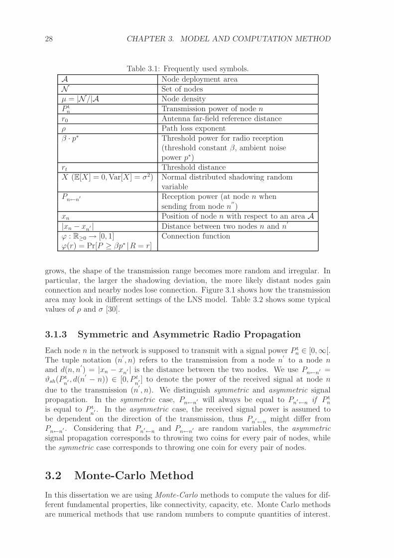
Table 3.1: Frequently used symbols.
A Node deployment areaN Set of nodesµ = |N /|A Node densityP tn Transmission power of node nr0 Antenna far-field reference distanceρ Path loss exponentβ · p∗ Threshold power for radio reception
(threshold constant β, ambient noisepower p∗)
rt Threshold distanceX (E[X] = 0,Var[X] = σ2) Normal distributed shadowing random
variablePn←n′ Reception power (at node n when
sending from node n′′)
xn Position of node n with respect to an area A|xn − xn′ | Distance between two nodes n and n
′
ϕ : R≥0 → [0, 1] Connection functionϕ(r) = Pr[P ≥ βp∗ |R = r]
grows, the shape of the transmission range becomes more random and irregular. Inparticular, the larger the shadowing deviation, the more likely distant nodes gainconnection and nearby nodes lose connection. Figure 3.1 shows how the transmissionarea may look in different settings of the LNS model. Table 3.2 shows some typicalvalues of ρ and σ [30].
3.1.3 Symmetric and Asymmetric Radio Propagation
Each node n in the network is supposed to transmit with a signal power P tn ∈ [0,∞[.
The tuple notation (n′, n) refers to the transmission from a node n
′to a node n
and d(n, n′) = |xn − xn′ | is the distance between the two nodes. We use Pn←n′ =
ϑsh(Ptn′ , d(n
′ − n)) ∈ [0, P tn′ ] to denote the power of the received signal at node n
due to the transmission (n′, n). We distinguish symmetric and asymmetric signal
propagation. In the symmetric case, Pn←n′ will always be equal to Pn′←n if P tn
is equal to P tn′ . In the asymmetric case, the received signal power is assumed to
be dependent on the direction of the transmission, thus Pn′←n might differ fromPn←n′ . Considering that Pn′←n and Pn←n′ are random variables, the asymmetricsignal propagation corresponds to throwing two coins for every pair of nodes, whilethe symmetric case corresponds to throwing one coin for every pair of nodes.
3.2 Monte-Carlo Method
In this dissertation we are using Monte-Carlo methods to compute the values for dif-ferent fundamental properties, like connectivity, capacity, etc. Monte Carlo methodsare numerical methods that use random numbers to compute quantities of interest.

3.2. MONTE-CARLO METHOD 29
0
0
(a) Shadowing with σ=2
0
0
(b) Shadowing with σ=4
Figure 3.1: Wireless transmission area of a sender at the center of a 400× 400 grid.Each point marks a position where the signal strength reaches a pre-defined constantthreshold
Environment ρ σOutdoor Free space 2 4 – 12
Shadowed/Urban 2.7 – 5Indoor Line-of-sight 1.6 – 1.8 3 – 6
Obstructed 4 – 6 6.8
Table 3.2: Some typical values of the path loss coefficient (ρ) and the shadowingdeviation (σ)
This is normally done by creating a random variable whose expected value is thedesired quantity. One then simulates the random variable and uses its sample meanto construct probabilistic estimates.
Assume Xn to be the random variable referring to the random position of noden and X = (X0, X1, X2, . . . , Xn) to be the random vector referring to a randomtopology. Any given property prop(X), which depends on the random node deploy-ment X, can thus implicitly also be considered as a random variable. The value ofinterest is the expected value of prop(X), namely E[prop(X)]. One could computeE[prop(X)] given the density function f(prop(X)) of the random variables prop(X).However, finding the density function with analytical methods is often not possible.But E[prop(X)] can approximately be computed using Monte-Carlo methods:
E[prop(X)] =
∫
R2N
E[prop(X)|X = x]p(X = x)dx
≈ 1
k
k−1∑
i=0
E[prop(X)|X = xi]
(3.2)
Or in other words, we approximately compute the expected value of prop(X) by sam-pling over k realizations of the underlying random network, with xi = (xi0, x
i1, x
i2, . . . , x
in)
as a concrete topology deployment.In the rest of the dissertation, we will use similar methods to approximately com-
pute expected values of specific properties like connectivity or capacity. Those prop-erties may, however, not only depend on the topology X, but also on other randomvariables like for instance the signal strength distribution or the traffic pattern.

30 CHAPTER 3. MODEL AND COMPUTATION METHOD

Chapter 4
Connectivity
Most work on connectivity has been done using the deterministic path loss model,which predicts the received power as a deterministic function of distance. It is knownthat the modelling the communication range as an ideal circle is not realistic. In real-ity, the received power at a certain distance is a random variable due to fading effects.This behavior is reflected by the shadowing model, as described in Equation 3.1. Inthis chapter, we study connectivity in wireless ad hoc networks using the shadowingradio propagation model. We first point out how radio irregularity affects the end-to-end connection probability and compare the results to measurements in the path lossmodel. In a second step, we study the correlation between the shadowing deviation(the parameter controlling the level of radio irregularity) and connectivity in moredetail and show that the log-normal shadowing model introduces an unnatural biasinto the analysis: as the shadowing deviation grows, the radio transmission range notonly becomes more irregular, but also enlarges. This naturally leads to an improvedconnectivity. In a third part, we obtain an unbiased view on the effects of radioirregularity on connectivity in a wireless network. We propose a method to eliminatethe bias introduced by the log-normal shadowing model. This allows us to capturethe intrinsic properties of radio irregularity and thus to compare different levels ofirregularity in a meaningful way. Our approach compensates for the enlarged radiotransmission range by adjusting the transmission power of the nodes accordingly.This technique is also used in percolation theory when comparing different networkmodels [68, 69, 70]. Overall, the results presented in this chapter are an importantcontribution since, when taken together, they show that an analysis of connectivityin a circular radio propagation model yields worst case bounds for connectivity.
4.1 Constant Transmission Power
4.1.1 Direct connection between nodes
Two nodes n and n′
can establish a direct communication link (n, n′) if the signal
strength of the received signal Pn←n′ at node n due to the transmission of node n′
is above a certain threshold value, namely Pn←n′ > β · p∗, where β is the thresholdconstant and p∗ the ambient noise power.
We define the threshold distance as the distance where the received signal power,when σ = 0, drops to the threshold value β · p∗. With respect to the shadowing radiopropagation model (Equation 3.1), the threshold distance is given by

32 CHAPTER 4. CONNECTIVITY
0.5 1 1.5 2
0.2
0.4
0.6
0.8
1
rrt
ϕLNS(r) = Pr[P ≥ βp∗ |R = r]
σ/ρ = 0.2σ/ρ = 0.5σ/ρ = 1σ/ρ = 2
Figure 4.1: Connection function for log-normal shadowing.
rt = r0
(
p0
βp∗
)1/
. (4.1)
The probability that a signal can be received correctly in distance r from a sendernode is given by the connection function ϕ(r). From 4.1, the connection function forthe log-normal shadowing radio propagation model calculates as1
ϕLNS(r) = Pr[P ≥ βp∗ |R = r] = Pr[
X ≥ 10ρ ln(r/rt)ln(10)
]
= 12− 1
2erf
(
10ρ ln(r/rt)√2 ln(10)σ
)
. (4.2)
The connection function is shown for different values of the shadowing deviationnormalized to the path loss exponent (σ/ρ), as the shape depends only on this ratio.For small values of σ/ρ, the connection function becomes a step function and theresulting network graph a unit disk graph with disks of radius r/rt = 1.
4.1.2 Impact of Shadowing on Connectivity
In this section we study how connectivity among nodes over multiple hops evolveswith an increasing shadowing deviation. For this, we first define the utility functionϕ : N ×N → 0, 1 with
ϕ(n, n′
) =
1 Pn←n′ > β · p∗0 otherwise.
(4.3)
.
The function ϕ(n, n′) computes to one if and only if a successful direct transmis-
sion from node n′to node n is possible.
We then say, two arbitrary nodes are connected in the network (possibly thoughmultiple hops), if there is a path between the nodes such that a successful transmissionbetween each two consecutive nodes is possible. Formally, this is described by theconnectivity ζn,n′ ∈ 0, 1 with
1The error function is defined for all real numbers x as erf(x) := 2√π
∫ x
0exp(−t2)dt.
4.1. CONSTANT TRANSMISSION POWER 33
ζn,n′ =
1 there is a path n0, n1, . . . , nz,with n0 = n and nz = n
′and
ϕ(ni+1, ni) = 1 for 0 ≥ i < z
0 otherwise.
(4.4)
.
In principal, ζn,n′ is a random variable since the position of nodes n and n′
israndom, as well as the positions and the signal strengths of all other nodes whichmay or may not participate the path.
We are interested in the expected value of ζn,n′ , for two arbitrary chosen nodes
n and n′. This corresponds to the following question. What is the probability of a
node to be able to communicate with a randomly chosen destination in the network.Finding the expected value of ζn,n′ using pure analysis is difficult. Adopting themethod described in Section 3.2, E[ζn,n′ ] can approximately be computed as follows.
ζ := E[ζn,n′ ] =
∫
R2N
E[ζn,n′ |X = x]p(X = x)dx
≈ 1
k
k−1∑
i=0
E[ζn,n′ |X = xi]
=1
k
k−1∑
i=0
1
|N |∑
n∈N
1
|N | − 1
∑
n′∈N\n
ζn,n′ |X=xi
=1
k · |N | · (|N | − 1)
k−1∑
i=0
∑
n∈N
∑
n′∈N\n
ζn,n′ |X=xi
(4.5)
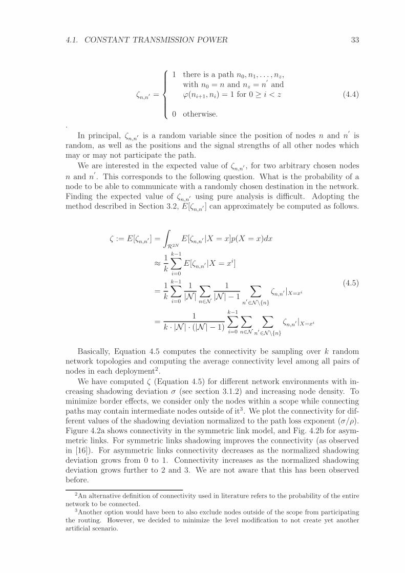
Basically, Equation 4.5 computes the connectivity be sampling over k randomnetwork topologies and computing the average connectivity level among all pairs ofnodes in each deployment2.
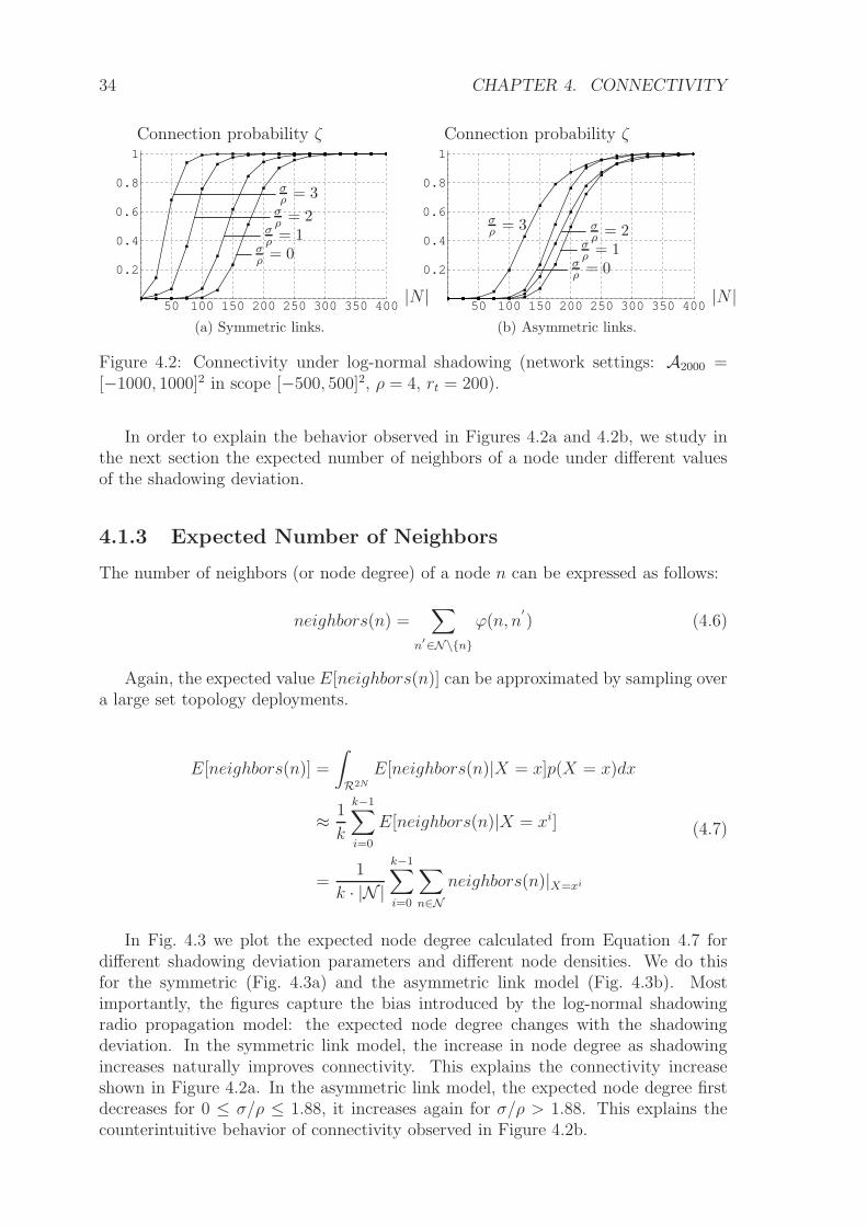
We have computed ζ (Equation 4.5) for different network environments with in-creasing shadowing deviation σ (see section 3.1.2) and increasing node density. Tominimize border effects, we consider only the nodes within a scope while connectingpaths may contain intermediate nodes outside of it3. We plot the connectivity for dif-ferent values of the shadowing deviation normalized to the path loss exponent (σ/ρ).Figure 4.2a shows connectivity in the symmetric link model, and Fig. 4.2b for asym-metric links. For symmetric links shadowing improves the connectivity (as observedin [16]). For asymmetric links connectivity decreases as the normalized shadowingdeviation grows from 0 to 1. Connectivity increases as the normalized shadowingdeviation grows further to 2 and 3. We are not aware that this has been observedbefore.
2An alternative definition of connectivity used in literature refers to the probability of the entirenetwork to be connected.
3Another option would have been to also exclude nodes outside of the scope from participatingthe routing. However, we decided to minimize the level modification to not create yet anotherartificial scenario.
34 CHAPTER 4. CONNECTIVITY
50 100 150 200 250 300 350 400
0.2
0.4
0.6
0.8
1
|N |
Connection probability ζ
σρ = 0
σρ = 1
σρ = 2
σρ = 3
(a) Symmetric links.
50 100 150 200 250 300 350 400
0.2
0.4
0.6
0.8
1
σρ = 1
|N |
Connection probability ζ
σρ = 0
σρ = 2
σρ = 3
(b) Asymmetric links.
Figure 4.2: Connectivity under log-normal shadowing (network settings: A2000 =[−1000, 1000]2 in scope [−500, 500]2, ρ = 4, rt = 200).
In order to explain the behavior observed in Figures 4.2a and 4.2b, we study inthe next section the expected number of neighbors of a node under different valuesof the shadowing deviation.
4.1.3 Expected Number of Neighbors
The number of neighbors (or node degree) of a node n can be expressed as follows:
neighbors(n) =∑
n′∈N\n
ϕ(n, n′
) (4.6)
Again, the expected value E[neighbors(n)] can be approximated by sampling overa large set topology deployments.
E[neighbors(n)] =
∫
R2N
E[neighbors(n)|X = x]p(X = x)dx
≈ 1
k
k−1∑
i=0
E[neighbors(n)|X = xi]
=1
k · |N |k−1∑
i=0
∑
n∈Nneighbors(n)|X=xi
(4.7)
In Fig. 4.3 we plot the expected node degree calculated from Equation 4.7 fordifferent shadowing deviation parameters and different node densities. We do thisfor the symmetric (Fig. 4.3a) and the asymmetric link model (Fig. 4.3b). Mostimportantly, the figures capture the bias introduced by the log-normal shadowingradio propagation model: the expected node degree changes with the shadowingdeviation. In the symmetric link model, the increase in node degree as shadowingincreases naturally improves connectivity. This explains the connectivity increaseshown in Figure 4.2a. In the asymmetric link model, the expected node degree firstdecreases for 0 ≤ σ/ρ ≤ 1.88, it increases again for σ/ρ > 1.88. This explains thecounterintuitive behavior of connectivity observed in Figure 4.2b.

4.2. ADAPTIVE TRANSMISSION POWER 35
0.5 1 1.5 2 2.5 3 3.5
1.5
2
2.5
3
3.5
4E[neighbors(n)] in scope [−800, 800]2
E[neighbors(n)] in scope [−1000, 1000]2
σ
(a) Symmetric links.
0.5 1 1.5 2 2.5 3 3.50.7
0.8
0.9
1
1.1 E[neighbors(n)] in scope [−800, 800]2
E[neighbors(n)] in scope [−1000, 1000]2
σ
(b) Asymmetric links.
Figure 4.3: Expected node degree under log-normal shadowing (network settings:A2000 = [−1000, 1000]2, N = 200, ρ = 4, rt = 200).
The figures also illustrate the boundary effects: the results considering the wholedeployment area differ quantitatively from those restricted to a smaller scope (asnodes close to the boundary have less neighbors).
These results show that log-normal shadowing primarily affects the node degree,which in turn affects connectivity. This is because an increasing shadowing deviationresults not only in a more irregular, but also in an enlarged radio transmission range,which is an unnatural side effect of the log-normal shadowing radio propagationmodel.
4.2 Adaptive Transmission Power
4.2.1 Connectivity Under Constant Node Degree
To avoid the effect of shadowing enlarging the transmission range we adjust thetransmission power of the nodes such that the expected node degree is kept constantfor different values of the shadowing deviation. To give some geometric intuition,this is equivalent to keeping the transmission area always the same regardless of theshape (and thus equal to a circle area for σ = 0).
We can compute the required power values which keeps the expected node degreeconstant as follows [71].
Corollary 4.1. In the log-normal shadowing radio propagation model on A∞ = R2,
the transmission powers p↔ and p such that
E[N↔]|p0=p↔ = E[N↔]|σ=0 (4.8a)
E[N]|p0=p= E[N]|σ=0 (4.8b)
are
p↔ = p0 exp(
− (ln(10)σ)2
100
)
(4.9a)
p = p0 exp(
− (ln(10)σ)2
100
) (
1− erf(
ln(10)σ10
))−
2 . (4.9b)
In Figure 4.4 we show how connectivity evolves (using Equation 4.5) with theshadowing deviation, this time using the transmission power (Equation 4.9) that

36 CHAPTER 4. CONNECTIVITY
50 100 150 200 250 300 350 400
0.2
0.4
0.6
0.8
1
|N |
Connection probability ζ
σ = 0
σ = 1
σ = 2
σ = 3
(a) Symmetric links.
50 100 150 200 250 300 350 400
0.2
0.4
0.6
0.8
1
σ = 2
|N |
Connection probability ζ
σ = 0
σ = 1
σ = 3
(b) Asymmetric links.
Figure 4.4: Connectivity under log-normal shadowing using the transmission powers4.9 that preserve the expected node degree (network settings: A2000 = [−1000, 1000]2
in scope [−500, 500]2, = 4, rt = 200).
preserves the expected node degree. Again, we consider both the symmetric (Figure4.4a) and the asymmetric link model (Figure 4.4b).
Our results demonstrate that connectivity increases with the shadowing deviationboth for symmetric and asymmetric links, if the expected node degree is kept constant.To the best of our knowledge this is the first result capturing the intrinsic impact ofradio irregularity on connectivity under log-normal shadowing. In the next sectionwe discover a plausible reason for the observed phenomenon: an increasing averageedge length.
4.2.2 Impact of Shadowing on Edge Length
To explore why connectivity increases with the shadowing deviation, even when thenode degree is kept constant, we study the distributions of distance between a ran-domly chosen pair of nodes (chosen either among all pairs of nodes or pairs that areconnected by an edge in the network graph, yielding the edge length distribution ofthe network graph).
More precisely, we consider the following experiment on a finite deployment areaAα = 1
2[−α, α]2: Randomly choose a pair of nodes that are connected by an edge (we
assume links to be symmetric throughout this section) and denote by R′ the distancebetween the two nodes. Let fR′(r) be the probability density function of R′.
In Figure 4.5 we plot the edge length distribution fR′(r) for different values of theshadowing deviation (be reminded that they are based on the transmission power ofEquation 4.9 that preserves the expected node degree). The figure illustrates howthe edge length distribution spreads out with shadowing and increasingly deviatesfrom a triangular distribution. This causes the average edge length to increase. Theincrease in the average edge length justifies the connectivity improvement caused byradio irregularity as observed in the previous section.
Our results indicate that — contrary to what intuition might suggest — radioirregularity is indeed beneficial for network connectivity.

4.3. SUMMARY 37
100 200 300 400 500 600 700
0.002
0.004
0.006
0.008
0.01
r
fR′(r)
σ/ = 0
σ/ = 1σ/ = 2
σ/ = 3
Figure 4.5: Edge length distribution under log-normal shadowing when using thetransmission power from 4.9 (network settings: A16000 = [−8000, 8000]2, N = 12800, = 4, rt = 200).
4.3 Summary
In this chapter we have studied the impact of log-normal shadowing on connectivityin wireless ad hoc networks.
We have shown that, when using the log-normal shadowing radio propagationmodel (LNS) to predict the reception power of transmissions in the network, the con-nectivity increases as the radio signal becomes more irregular. Mainly, this is becausethe expected node degree increases as the shadowing deviation (the parameter of theLNS model controlling the level of radio irregularity) increases. In order to providea fair comparison among different levels of radio irregularity, we have computed net-work connectivity using an adjustment of the transmission power of the nodes thatkeeps the expected node degree constant. Our results show that even under thosecircumstances connectivity improves. This is of interest for many existing bounds onthe connectivity of wireless networks that have been derived using the deterministicpath loss model, as our results indicate these are lower instead of upper bounds onconnectivity.

38 CHAPTER 4. CONNECTIVITY

Chapter 5
Capacity: Model
Throughput capacity is another important property of wireless networks. As withconnectivity, it is difficult to find closed expressions for the capacity of a wirelessnetwork, and even more complicated to analytically study the effects of realisticphysical layer models. In this chapter we present a model for throughput capacitythat can be used to compute capacity numerically. The approach chosen has a two-fold advantage: it is protocol independent and, at the same time, it allows to studyeffects of various physical layer properties. Experiments using the model will bepresented in chapter 7.
5.1 Overview
The main factor that limits capacity in wireless networks is interference, a conse-quence of using a shared communication medium. An accurate modeling of interfer-ence is fundamental in order to derive results of practical relevance. In the literature,two main interference models have been proposed [17]: the protocol and the physicalinterference model. In the protocol model, a transmission from a node u is said to bereceived successfully by another node v if no node w closer to the destination nodeis transmitting simultaneously. However, in practice, nodes outside the interferencerange of a receiver might still cause enough cumulated interference to prevent thereceiver from decoding a message from a given sender. This behavior is capturedby the physical model, where a communication between nodes u and v is successfulif the SINR (Signal to Interference plus Noise Ratio) at v (the receiver) is above acertain threshold. The physical model can also be less restrictive than the protocolmodel in a sense that a message from a node u might be correctly received by node veven if there is a simultaneously transmitting node w close to v; for instance becauseu is using a much larger transmission power than node w. Practical measurementshave shown [15, 12] that in some cases a node v might also experience a strongersignal from a node w farther away than another node u, even if both nodes u and wtransmit at the same power level. Thus, an accurate modeling of signal propagationis as well important when computing capacity in wireless networks. Similar as donein chapter 4, we use the log-normal shadowing radio propagation (see section 3.1.2)to model the signal propagation in the most realistic way.
Analytical studies on capacity in the presence of realistic radio propagation andinterference models – such as log-normal shadowing and physical interference – are
40 CHAPTER 5. CAPACITY: MODEL
Notation Semantic
ψ channel assignment functionκ interference modelΓ set of channelsDn set of nodes that can be decoded at node n without noiseUn set of nodes that can be decoded at node n under noiseE set of directed edges in a schedule graphGT (N , E) schedule graph
ω(n′, n) weight function indicating the number of channels
used on a linkΥ set of source destination pairsη routing functionBn′ ,n lowest number of channels between any two neighbors
along a pathT used channels, T = |Γ| in GT (N , E)λn′ ,n achievable throughput capacity along a path
λ expected throughput capacity of the network
Table 5.1: Notation
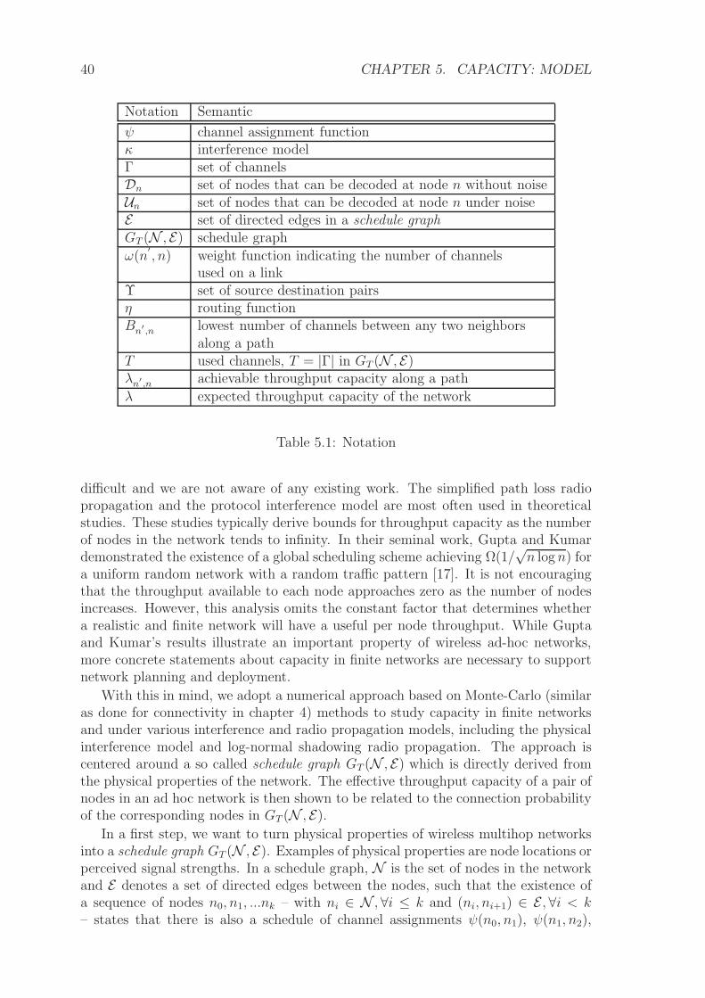
difficult and we are not aware of any existing work. The simplified path loss radiopropagation and the protocol interference model are most often used in theoreticalstudies. These studies typically derive bounds for throughput capacity as the numberof nodes in the network tends to infinity. In their seminal work, Gupta and Kumardemonstrated the existence of a global scheduling scheme achieving Ω(1/
√n logn) for
a uniform random network with a random traffic pattern [17]. It is not encouragingthat the throughput available to each node approaches zero as the number of nodesincreases. However, this analysis omits the constant factor that determines whethera realistic and finite network will have a useful per node throughput. While Guptaand Kumar’s results illustrate an important property of wireless ad-hoc networks,more concrete statements about capacity in finite networks are necessary to supportnetwork planning and deployment.
With this in mind, we adopt a numerical approach based on Monte-Carlo (similaras done for connectivity in chapter 4) methods to study capacity in finite networksand under various interference and radio propagation models, including the physicalinterference model and log-normal shadowing radio propagation. The approach iscentered around a so called schedule graph GT (N , E) which is directly derived fromthe physical properties of the network. The effective throughput capacity of a pair ofnodes in an ad hoc network is then shown to be related to the connection probabilityof the corresponding nodes in GT (N , E).
In a first step, we want to turn physical properties of wireless multihop networksinto a schedule graph GT (N , E). Examples of physical properties are node locations orperceived signal strengths. In a schedule graph, N is the set of nodes in the networkand E denotes a set of directed edges between the nodes, such that the existence ofa sequence of nodes n0, n1, ...nk – with ni ∈ N , ∀i ≤ k and (ni, ni+1) ∈ E , ∀i < k– states that there is also a schedule of channel assignments ψ(n0, n1), ψ(n1, n2),
5.2. NODE RELATIONSHIPS 41
...ψ(nk−1, nk) in a way that node n0 is able to consecutively transmit data to nodenk at a rate λn0,nk
> 0. The idea behind building a schedule graph is to createan abstraction that allows us to deduce the achievable capacity of the underlyingwireless network. In this section, we first define some common properties in order togradually develop the graph representation. A list of all the notations used withinthe following two sections, including the aforementioned sets of nodes, can be foundin Table 5.1. Throughout this chapter, we use P(·) to refer to the collection of allpossible subsets of a set.
5.2 Node Relationships
Whether a signal from a node n′ can be decoded correctly at node n in the absence,or the presence, of concurrent transmissions, is determined by the interference model.In this work, we assume interference models to be defined by a binary interferencefunction κ : N × N × P(N) −→ 0, 1 with
κ(n′
, n, In′ ) =
1 The signal of n′can be decoded at
node n under a set In′ of concurrentlytransmitting nodes
0 otherwise.
(5.1)
The interference function for the protocol model [17] looks like
κprotocol(n′
, n, In′ ) = 1 ⇔ d(n′′
, n) > d(n′, n), ∀n′′ ∈ In′ (5.2)
and for the physical interference model [17] as follows:
κsinr(n′
, n, In′ ) = 1 ⇔ Pn←n′
P ∗n +∑
n′′∈In′Pn←n′′
> βsinr (5.3)
for some threshold βsinr and P ∗n as the thermal noise perceived at node n. Anotherinterference model which is related to the CSMA/CA behavior of 802.11 is the diskinterference model. Under disk interference,
κdisk(n′
, n, In′ ) = 1 ⇔ d(n′′
, n) > RI , ∀n′′ ∈ In′ (5.4)
where RI is called interference range. The disk model is often used in network simu-lators such as NS-2 [72]. Typical values for RI are in between 1.5 and 2.5 times thetransmission range. We now assign two sets of nodes to each node n ∈ N , namelyDn and Un.
Dn = n′ ∈ N | κ(n′
, n, ∅) = 1 (5.5)
is the set of nodes that can be correctly decoded at node n in the absence of anyother concurrent transmission.
Un = n′ ∈ D | κ(n′
, n, In′ ) = 1 (5.6)
contains all nodes n′
that can be correctly decoded at node n in the presence ofa set of nodes In′ transmitting concurrently as node n
′. For later use we define
D = (n′, n) | n′ ∈ Dn, ∀n ∈ N to be the set of all transmissions in the network
when interference is ignored, and U = (n′, n) | n′ ∈ Dn, ∀n ∈ N to be the set of all
transmissions in the network if interference is considered.
42 CHAPTER 5. CAPACITY: MODEL
e1
Network Interference Conflicts Channels
e2
e3
n12 2
36
7
e1 e2
e3 e4
0 1
0 0
Figure 5.1: Channel assignment under protocol interference.
Algorithm 5.1 Conflict graph under protocol interference
Input: Set of all transmissions DOutput: Set of conflicts C ⊆ (e, e′) | e, e′ ∈ D
1: C := ∅;2: for all e := (n
′
, n) ∈ D do3: for all n
′′ ∈ N\n, n′ do4: if d(n
′′
, n) ≤ d(n′, n) then5: Q := (n′′
, n′′′
) | n′′ ∈ Dn′′′
6: for all e′ ∈ Q do
7: C := C ∪ (e′ , e), (e, e′);8: end for9: end if
10: end for11: end for
5.3 Scheduling Algorithms
Which transmissions in the network occur simultaneously is determined by the schedul-ing algorithm. In our model, we assume the medium to be divided into a set ofchannels ψi. Each channel can be seen as a set of directed transmissions (n′, n), withn
′ ∈ Dn, between two nodes n′ and n. Channels have to be assigned to transmissionsin a way such that no two transmissions scheduled within the same channel interfere.At the same time, one wants to keep the number of channels used as low as possible.This is trivial for the protocol and the disk model, but turns out to be more difficultunder the physical interference model. In general, the problem of scheduling is relatedto the traditional graph coloring problem, except that the vertices in the graph to becolored refer to the transmissions in the network and the edges in the graph refer tothe interference conflicts. Two vertices conflict if their corresponding transmissionscannot be scheduled simultaneously. We call such a graph a conflict graph.
For the protocol model, building a conflict graph is straightforward as shown inAlgorithm 5.1. A conflict between two transmissions (n′, n), (n
′′′, n
′′) exists whenever
either d(n′′′, n) < d(n
′, n) or d(n
′, n
′′) < d(n
′′′, n
′′), where d(·, ·) is the distance func-
tion d(n′, n) = |xn− xn′ |. Conflict graph construction and channel assignment under
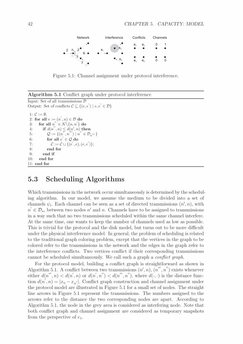
the protocol model are illustrated in Figure 5.1 for a small set of nodes. The straightline arrows in Figure 5.1 represent the transmissions. The numbers assigned to thearrows refer to the distance the two corresponding nodes are apart. According toAlgorithm 5.1, the node in the grey area is considered as interfering node. Note thatboth conflict graph and channel assignment are considered as temporary snapshotsfrom the perspective of e1.

5.3. SCHEDULING ALGORITHMS 43
e1
Network Interference Conflicts Channels
e2
e3
n1
n1
e1 e2
e3 e4
0 1e4
n2
0 0
Figure 5.2: Channel assignment under disk interference.
Algorithm 5.2 Conflict graph under disk interference
Input: Set of all transmission D, interference range RI
Output: Set of conflicts C ⊆ (e, e′) | e, e′ ∈ D
1: C := ∅;2: for all e := (n
′
, n) ∈ D do3: for all n
′′ ∈ N\n, n′ do4: if d(n
′′
, n) ≤ RI then5: Q := (n′′
, n′′′
) | n′′ ∈ Dn′′′
6: for all e′ ∈ Q do
7: C := C ∪ (e′ , e), (e, e′);8: end for9: end if
10: end for11: end for
The procedure is similar in the disk model (Algorithm 5.2), where a conflictbetween two transmissions (n′, n), (n
′′′, n
′′) exists whenever either d(n
′′′, n) < RI
or d(n′′, n
′) < RI , where RI is the interference range. An example of a conflict
graph and channel assignment under disk interference is given in Figure 5.2. Thestraight line arrows in Figure 5.2 represent the transmissions. The disk centered atnode n1 refers to the interference range with radius RI , compliant with Equation5.4. According to Algorithm 5.2, nodes in the grey area are considered as interferingnodes. Transmissions e3 and e4 do not conflict with e1 because node n1 and n2 arenot included in the grey area.
In the physical model, conflicts between two transmissions cannot be determinedwithout considering all other transmissions. As an example, two nodes in distance 2dmay interfere with a transmission at distance d if their interference is accumulated.For a node n
′to belong to Un, κphysical(n′
, n,N \ Cn←n′ ) must compute to 1, givenCn←n′ contains all nodes n
′′acting as a sender in a transmission that conflicts with
the transmission (n′, n).
In practice, of course, one wants to find the minimum set Cn←n′ of conflicts for atransmission (n
′, n), because this minimizes the number of channels to be used at a
later point in time. How to compute the minimum set of conflicts for a given set oftransmissions D in the physical interference model is shown in Algorithm 5.3. For agiven transmission (n
′, n), the algorithm operates by gradually testing the SINR ratio
with an increasing set of interferer, starting with the node contributing the lowestsignal power. At the point where the cumulated interference of a node n
′′leads to
a SINR ratio smaller than βsinr, all transmitting nodes n′′′
with Pn←n′′′ ≥ Pn←n′′
are considered as interferer and their associated transmissions are defined as conflictswith (n
′, n).

44 CHAPTER 5. CAPACITY: MODEL
e1
e1 e2
e3
Network Interference Conflicts Channels
e2
e3
n1
8 6
2
2
36
e4
e4
0 1
0 1
n2
Figure 5.3: Channel assignment under physical interference.
Algorithm 5.3 Conflict graph under physical interference
Input: Set of all transmission DOutput: Set of conflicts C ⊆ (e, e′) | e, e′ ∈ D
1: C := ∅;2: for all e := (n
′
, n) ∈ D do3: L := sort(N\n′
, n) such that n′′ ≺ n′′′ ←→ Pn←n
′′ < Pn←n′′′
4: M∗ := ∅;5: for all n
′′ ∈ L do6: M∗ :=M∗ ∪ n′′7: if κsinr(n
′
, n,M∗) = 0 then8: Q := (n′′
, n′′′
) | n′′ ∈ Dn′′′
9: for all e′ ∈ Q do
10: C := C ∪ (e′ , e), (e, e′);11: end for12: end if13: end for14: end for
We have shown how a conflict graph can be built for the different interferencemodels. Based on the conflict graph, efficient coloring algorithms might be used toassign channels to the transmissions (represented as nodes in the conflict graph).Finding the minimum number of channels, however, is an NP hard problem andthus is not feasible for large networks [73]. We decided to apply a Greedy channelassignment algorithm (Algorithm 5.4). Algorithm 5.4 assigns channels to transmis-sions in a greedy way, so that no two transmission e1, e2 will be scheduled using thesame channel if there exists a conflict between the two transmissions ((e1, e2) ∈ C).Algorithm 5.4 further assigns channels in a traffic proportional way, meaning thateach node pair (n
′, n), with n
′ ∈ Dn, is assigned exactly as many channels as thereare flows occupying the wireless link. Conflict graph and channel assignment for thephysical interference model are illustrated in Figure 5.3 in a small example network.The straight line arrows in Figure 5.3 represent the transmissions. The dotted ar-rows denote signals which contribute to the interference noise of transmission e1. Theweight assigned to an edge corresponds the signal strength. We assume the thermalnoise P ∗ and βsinr used in Equation 5.3 to be 1. According to Algorithm 5.3, nodesin the grey area are considered as the smallest set of nodes such that the remainingcumulated interference does not prohibit transmission e1 to be established. There isno conflict between transmissions e1 and e3 because node n1 is not included in thegrey area. Note that both conflict graph and channel assignment are considered assnapshots from the perspective of e1.

5.4. SCHEDULE GRAPH 45
Algorithm 5.4 Greedy channel assignment
Input: Set of all transmission D, set of conflicts COutput: Set of channels ψ0, ψ1, ..., ψT−1 with ψi ⊆ D
1: for all e ∈ D do2: for i := 0; i < µ(e) do3: Q := e′ | (e, e′) ∈ C4: Ω := ∅;5: for all e
′ ∈ Q do6: Ω := Ω ∪ ψi | e
′ ∈ ψi7: end for8: ψi := freechannel(Ω);9: ψi := ψi ∪ e;
10: end for11: end for
freechannel(Q)
1: Ω∗ := sort(Q) such that ψi ≺ ψj ←→ id(ψi) < id(ψj)2: i := −13: for all ψ ∈ Ω do4: if id(ψ) > i+ 1 then5: break;6: end if7: i := id(ψ);8: end for9: return ψi+1;
5.4 Schedule Graph
Coming back to the definition of Un, we can say, a node n′
belongs to Un if In′ inEquation 5.6 is defined as the set of nodes transmitting in the same channel as noden
′. Given a schedule and the set Un for each node, we define a so called schedule
graph as a directed and weighted graph GT (N , E), where E denotes the set of directededges with
E = (n′
, n) ∈ N ×N | n′ ∈ Un ∧ n ∈ Dn′. (5.7)
The set E includes all transmissions (n′, n) whose signals can be decoded correctly at
node n under interference, while the reverse signal might only be correctly decoded ifthere is no interference1. The subscript T indicates the number of channels used (Al-gorithm 5.4). The weight of an edge (n
′, n) ∈ E is given by ω(n
′, n), the transmission
capacity function.
ω(n′
, n) =∑
γ∈ψ(n′ ,n)
κ(n′
, n, Iγ). (5.8)
Here, Iγ denotes the set of nodes transmitting during channel γ, or Iγ = n′ ∈ N |γ ∈ ψ∗(n′
).It follows directly from the definition of a schedule graph GT (N , E) that for any
path n0, n1, ...nk – with ni ∈ N , ∀i ≤ k and (ni, ni+1) ∈ E , ∀i < k – there is alsoa corresponding schedule of channel assignments ψ(n0, n1), ψ(n1, n2), ...ψ(nk−1, nk)
1Note that Equation 5.7 models the acknowledgment as an infinite small packet not occupyingthe medium

46 CHAPTER 5. CAPACITY: MODEL
in a way that node n0 is able to consecutively transmit data to node nk at a ratestrictly greater than zero. We will make use of this property later when deducing theachievable capacity of the underlying physical network.
5.5 Throughput Capacity
Throughout this section, an ad hoc network is represented by its schedule graphGT (N , E) with the corresponding weight function ω. Capacity is then defined over agiven traffic pattern Υ:
Υ ⊆ (n′
, n) ∈ N ×N|n′ 6= n. (5.9)
More precisely, we want to know, for a schedule graph GT (N , E) and a traffic patternΥ, what is the end-to-end throughput capacity λn′
,n a given communication pair
(n′, n) ∈ Υ will perceive.
Important to the computation of throughput capacity is the routing function η :N × N −→ P(E). Hence, for a given source-destination pair (n
′, n) the resulting
route simply consists of the set of edges2 included in the sequence e0, e1...ek−1, withei = (ni, ni+1) ∈ E and n0 = n
′and nk = n.
Now consider the fact that in a schedule graph, a path between two nodes alsoreflects a schedule of channels. Throughput capacity is a concave metric, meaningthat the available throughput for a certain source destination pair is always deter-mined by the node with the lowest bandwidth, the so called bottleneck. Hence, letB∗n′ ,n
= mine∈η(n′ ,n) ω(e) be a random variable indicating lowest number of channels
available between two nodes along the path from n′to n. One can easily verify that
the resulting throughput capacity along the path can not be bigger than W ·B∗n′,n/T ,
where W is the maximum transmission rate equal to all nodes and T =| Γ | is thenumber of channels used in total.
The throughput capacity may be further diminished when considering all thetraffic Υ taking place in the network. For this purpose let us define a so called loadfunction µ : E −→ [0, N ], indicating to what extent a certain edge e ∈ E is sharedamong other ongoing traffic, or more formally:
µ(e) =∑
i=η(n′,n)
(n′,n)∈Υ
1i(e) (5.10)
where 1i : E −→ 0, 1 is the set membership function. If we want to take all ongoingtraffic into account we therefore have to consider µ while computing B∗
n′ ,n, or
Bn′ ,n =
0 η(n′, n) = ∅
mine∈η(n′ ,n)ω(e)µ(e)
otherwise.(5.11)
Based on the definition of Bn′ ,n we now claim that the achievable throughput λn′ ,n
for a communication pair (n′, n) ∈ Υ in a schedule graph GT (N , E) can be modelled
as
2Since we assume no loops and the order of the edges in a route is not important for the compu-tation of λ, we prefer the set notion which simplifies further treatment.

5.6. SUMMARY 47
λn′ ,n =W · Bn′ ,n
T. (5.12)
In a simplified setup, where each node is only allowed to transmit within one singlechannel, Bn
′,n refers to the path availability between n
′and n in GT (N , E) and
therefore λn′ ,n can be seen as a direct function of the connection probability betweenthe two nodes. Or one can say that the capacity of an ad hoc network is related to theconnectivity of its corresponding schedule graph GT (N , E). This might be of interestwhen analyzing capacity in sparse and partially disconnected random networks, butalso in mobile scenarios where the movement of the nodes often leads to temporarilybroken paths.
Since both the network and its graph representation GT (N , E) are random, obvi-ously the resulting throughput per node pair λn′ ,n can also be considered as random.Similar as done in chapter 4 we use Monte-Carlo methods to approximately computethe expected value of E[λn′ ,n] of the random variable λn′ ,n:
E[λn,n′ ] =
∫
R2N
E[λn,n′ |X = x]p(X = x)dx
≈ 1
k
k−1∑
i=0
E[λn,n′ |X = xi]
=1
k
k−1∑
i=0
1
|Υ|∑
(n,n′)∈Υ
λn,n′ |X=xi
=1
k · |Υ|k−1∑
i=0
∑
(n,n′)∈Υ
λn,n′ |X=xi
(5.13)
Or in other words, we approximately compute E[λn′ ,n] by sampling over k realiza-tions of the underlying random network while using the mean throughput capacitycomputed over all communication pairs (n, n
′ ∈ Υ). In Equation 5.13 xi refers to aconcrete set of node placements in the area A.
5.6 Summary
In this chapter, we presented a model for studying throughput capacity of wirelessmulti-hop networks under realistic settings. Contrary to existing work, looking atcapacity from an asymptotic perspective based on simplified network models (e.g.,protocol interference, unidirectional links, perfect scheduling or straight line routing),our approach analyzes capacity for finite networks under more realistic network con-figurations. In our model, the effective throughput of a random network is consideredas a random variable depending on the node distribution, the communication pattern,the radio propagation, channel assignment, etc..

48 CHAPTER 5. CAPACITY: MODEL

Chapter 6
Capacity: Validation
In this chapter, we use the model developed in chapter 5 to study capacity under veryspecific network topologies. We compare our results to results obtained through realmeasurements and ns-2 simulations [72]. By doing so, we validate our model while atthe same time we show the difference between protocol specific throughput capacity(real measurements or simulation based on IEEE802.11) and protocol independentthroughput capacity.
6.1 Capacity of static networks
To validate the model, we compute the throughput capacity of two simple; staticscenarios, static in the sense that the network topology as well as the communicationpattern is fixed. The throughput of such fixed network configurations can be seenas the conditional expected value E[λn,n′ |X = x] of the random variable λn,n′ undera concrete node placement x. For a fixed channel assignment ψ, we simply useE[λn,n′ |X = x] = 1
|Υ|∑
(n′ ,n)∈Υ λn,n′ |X=xi, where xi is the given set of coordinates
of the nodes. For both examples we will consecutively derive E[λn,n′ |X] by goingthrough the basic steps of sections 5.2 – 5.5.
The first network topology we consider consists of three nodes being distance dapart from each other, as shown in Figure 6.1a. To simplify the analysis, we usethe more primitive protocol interference model as described in Equation 5.2. Let usfurther assume n
′ ∈ Dn for all n′ 6= n. According to κprotocol, the set of senders Un is
modeled in a way that a node n′belongs to Un if, and only if, no other concurrent
transmission with a signal stronger than Pn←n′ is received by node n. Hence, thegraph GT only depends on how the different channels are assigned to the nodes.We now want to illustrate the outcome of E[λn,n′ |X = x] for three possible channelassignments. We keep track of all states and sets of the network model for each ofthe three channel assignments in Table 6.1.
In all the configurations we assume shortest path routing and only assign channelsto edges that are also used when considering the traffic pattern Υ. In the case ofone common channel ψ(n
′, n) = ψ(n, n
′) for all nodes n, n
′, no transmission can
correctly be decoded at any receiver (Equation 5.2) which leads to Un = ∅, E = ∅,Sn,n′ = 0, λn,n′ = 0 and finally to E[λn,n′ |X = x] = 0. In the presence of two separatechannels (T = 2), two directed links can be established (among the potential 6).Along with a communication pattern Υ = (A,B), (B,C), (C,A) (see Table 6.1),
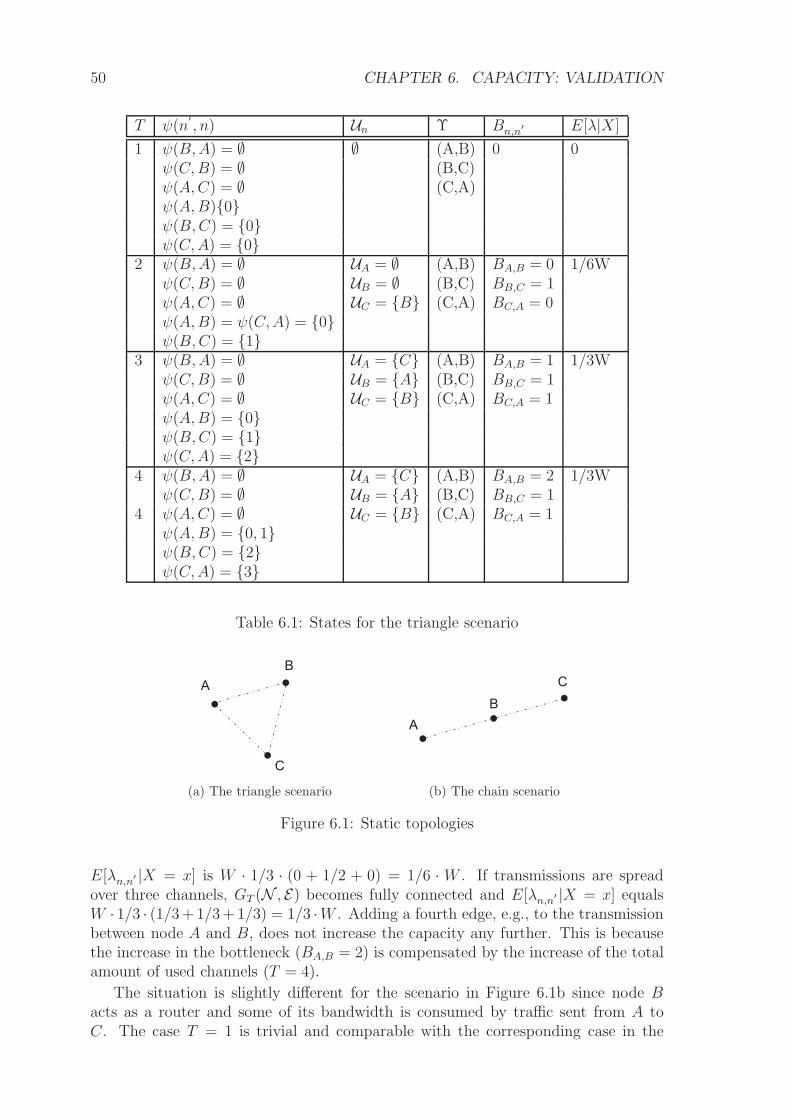
50 CHAPTER 6. CAPACITY: VALIDATION
T ψ(n′, n) Un Υ Bn,n′ E[λ|X]
1 ψ(B,A) = ∅ ∅ (A,B) 0 0ψ(C,B) = ∅ (B,C)ψ(A,C) = ∅ (C,A)ψ(A,B)0ψ(B,C) = 0ψ(C,A) = 0
2 ψ(B,A) = ∅ UA = ∅ (A,B) BA,B = 0 1/6Wψ(C,B) = ∅ UB = ∅ (B,C) BB,C = 1ψ(A,C) = ∅ UC = B (C,A) BC,A = 0ψ(A,B) = ψ(C,A) = 0ψ(B,C) = 1
3 ψ(B,A) = ∅ UA = C (A,B) BA,B = 1 1/3Wψ(C,B) = ∅ UB = A (B,C) BB,C = 1ψ(A,C) = ∅ UC = B (C,A) BC,A = 1ψ(A,B) = 0ψ(B,C) = 1ψ(C,A) = 2
4 ψ(B,A) = ∅ UA = C (A,B) BA,B = 2 1/3Wψ(C,B) = ∅ UB = A (B,C) BB,C = 1
4 ψ(A,C) = ∅ UC = B (C,A) BC,A = 1ψ(A,B) = 0, 1ψ(B,C) = 2ψ(C,A) = 3
Table 6.1: States for the triangle scenario
A
B
C
(a) The triangle scenario
A
B
C
(b) The chain scenario
Figure 6.1: Static topologies
E[λn,n′ |X = x] is W · 1/3 · (0 + 1/2 + 0) = 1/6 · W . If transmissions are spreadover three channels, GT (N , E) becomes fully connected and E[λn,n′ |X = x] equalsW · 1/3 · (1/3+1/3+1/3) = 1/3 ·W . Adding a fourth edge, e.g., to the transmissionbetween node A and B, does not increase the capacity any further. This is becausethe increase in the bottleneck (BA,B = 2) is compensated by the increase of the totalamount of used channels (T = 4).
The situation is slightly different for the scenario in Figure 6.1b since node Bacts as a router and some of its bandwidth is consumed by traffic sent from A toC. The case T = 1 is trivial and comparable with the corresponding case in the

6.2. CAPACITY OF LARGER NETWORKS 51
Table 6.2: States for the chain scenario
T ψ(n′, n) Un Υ Bn,n
′ E[λ|X]
2 ψ(A,B) = ψ(C,B) = 0 UA = B (A,B) BA,B = 0 1/6Wψ(B,C) = 1 UB = ∅ (B,C) BB,C = 1ψ(B,A) = ∅ UC = B (C,A) BC,A = 0
3 ψ(A,B) = 0 UA = B (A,B) BA,B = 1 2/9Wψ(B,C) = 1 UB = A (B,C) BB,C = 1ψ(C,B) = ψ(B,A) = 2 UC = B (C,A) BC,A = 0
4 ψ(A,B) = 0 UA = B (A,B) BA,B = 1 1/4Wψ(B,A) = 1 UB = A,C (B,C) BB,C = 1ψ(B,C) = 2 UC = B (C,A) BC,A = 1ψ(C,B) = 3
(A,C) BA,B = 1/2 1/6W(B,C) BB,C = 1/2(C,A) BC,A = 1
5 ψ(A,B) = 0 UA = B (A,C) BA,B = 1 1/5Wψ(B,A) = 1 UB = A,C (B,C) BB,C = 1ψ(B,C) = 2, 3 UC = B (C,A) BC,A = 1ψ(C,B) = 4
triangle scenario. Assigning two channels to the four edges results in two estab-lished links (UA = B and UC = B). Considering the traffic pattern Υ, it issufficient for one path to be established (e.g., SB,C = 1) and the resulting capacityE[λn,n′ |X = x] computes to 1/6 · W . Two of the three routes can be establishedif 3 channels are used (T = 3), which results in E[λn,n′ |X = x] = 2/9 · W . Thecapacity of the given traffic pattern can be further improved by assigning one chan-nel per transmission pair. All the routes can be established with a bottleneck ofBn,n′ = 1, ∀(n, n′
) ∈ Υ and E[λn,n′ |X = x] equals 1/4 · W . Obviously, the samechannel assignment results in a different capacity if another traffic pattern is used,like, e.g. Υ = (A,C), (B,C), (C,A). Since the link between node B and C is usedtwice, the values for BA,C BB,C reduce to 1/2. For such a traffic pattern, a 5-channelassignment performs better, as shown in Table 6.2.
6.2 Capacity of larger networks
In this section we analyze throughput capacity of various types of communicationpatterns and network topologies. To simplify the notation we will refer to E[λn,n′ ]as λ for the rest of the dissertation. For each analyzed configuration we also pro-vide results taken from simulations with ns-2 [72] using the very same topology andcommunication setup. Throughout this section, we use log-normal shadowing radiopropagation with σ = 0 and ρ = 2, and a SINR based interference model, κsinr,as described in Equation 5.3. Since σ is 0, the threshold for a node n
′to be part
of Dn only depends on the distance between the two nodes. We have set P ∗n of

52 CHAPTER 6. CAPACITY: VALIDATION
0
0.2
0.4
0.6
0.8
1
2 3 4 5 6 7 8 9 10
thro
ugh
put
capac
ity
nodes
λns-2
(a) Vis-a-vis traffic
0
0.2
0.4
0.6
0.8
1
2 3 4 5 6 7 8 9 10
thro
ugh
put
capac
ity
nodes
λns-2
(b) Random traffic
Figure 6.2: Chain topology
Equation 5.3 such that n′ ∈ Dn ⇔ |xn′ − xn| ≤ 250. To avoid mixing up capacity
measurements with routing issues, packets within ns-2 simulations are forwarded us-ing pre-computed shortest path routes. We further have set the MAC data rate inns-2 to 1Mbit/sec. This is necessary since operating 802.11 at higher rates resultsin drastically reduced efficiency and makes the measurements difficult to compare asthe per-packet overhead dominates the overall cost. This is due to the fixed length802.11 preamble used by the hardware for bit synchronization.
6.2.1 Chain
In a first comparison we look at a configuration of a chain of n nodes. Each node is200 meters away from its neighbor. The first node acts as a source of data traffic,the last node is the traffic sink. Data is sent as fast as the MAC allows. Since thereare no random components involved, λ is a direct function of the channels needed,and computes to 1/4 as the chain grows. From Figure 6.2a, we see that the value ofλ lies above the throughput measured with ns-2, especially when the chain becomeslarge. This is due to the overhead of headers, RTS, CTS and ACK packets, but alsobecause in reality nodes fail to achieve an optimal schedule. The results obtainedwith our model match those presented in [19], where the authors discuss throughputcapacity measurements taken from ns-2 simulations with respect to theoretical upperbounds.
As a more realistic scenario, we now investigate random communication patternsin chain topologies. For this purpose, we assign a random destination d(n) ∈ N\nto every node n ∈ N . Figure 6.2b shows the effect of such a traffic pattern onthroughput. The plot shows quite a close match between λ and the measurementsobtained with ns-2. This is not too surprising since we know from Figure 6.2a thatthe throughput of an 802.11 chain tallies with the theoretical limit if the chain lengthis short. Under a random communication pattern the average path length in a chainis far below the maximum value of n − 1, for a chain of length n. Furthermore,overlapping communication paths reduce capacity (Bn,n′ in our model) due to theforwarding load inflicted upon the nodes, especially if the chain becomes long.

6.2. CAPACITY OF LARGER NETWORKS 53
0
0.05
0.1
0.15
0.2
0.25
0.3
0 10 20 30 40 50 60 70 80 90 100
thro
ugh
put
capac
ity
nodes
λns-2
(a) Cross traffic
0
0.05
0.1
0.15
0.2
0.25
0.3
0 10 20 30 40 50 60 70 80 90 100
thro
ugh
put
capac
ity
nodes
λns-2
(b) Random traffic
Figure 6.3: Grid topology
6.2.2 Grid
We look at grid topologies where each node is 200 meters away from its closestneighbor and the nodes communicate using a random communication pattern. Figure6.3a shows the capacity in the grid topology for a cross communication pattern:source nodes in the first column have a destination assigned in the corresponding rowin the last column, and source nodes in the first row have a destination assigned inthe corresponding column in the last row. From Figure 6.3a we see that the modelbased computation predicts a higher throughput capacity than the one measuredwith ns-2. This is because the cross communication pattern is actually composed ofend-to-end chain communications exactly like the scenario used to compute Figure6.2a. We know that for large chain communications, 802.11 throughput capacity isfar below the model-based capacity, for reasons explained in section 6.2.1. In the gridtopology with cross communication this behavior is amplified. Figure 6.3b showsthe capacity in the grid for a random communication pattern where each node getsassigned a random destination. Similarly to the chain example, the gap betweenns-2 measurements and results obtained through our model disappears slightly whencommunication becomes random. Random communication reduces the average pathlength and therefore diminishes the impact of the suboptimal channel assignment andthe header overhead inherent in 802.11.
6.2.3 Random Topology
We consider random topologies of n nodes distributed uniformly within an area of1000 × 1000 square meters. Each node n acts as a traffic generator and has a ran-dom destination assigned, chosen uniformly out of N\n. Figure 6.4a shows thethroughput capacity λ in contrast with ns-2 simulation measurements. Similar as inthe chain and the grid scenario, the model based prediction matches quite well withthe ns-2 simulations. The result supports the trend already observed in the previousconfigurations of the chain and the grid: the higher the randomness in topology andcommunication, the better the throughput approximation is. This might particularlybe the case in dense networks where the demand for channels is high due to the highnode degree, leaving less room for an optimal channel assignment.

54 CHAPTER 6. CAPACITY: VALIDATION
0
0.05
0.1
0.15
0.2
10 20 30 40 50 60 70 80 90 100
thro
ugh
put
capac
ity
nodes
λns-2
Figure 6.4: Random topology
0
1
2
3
4
5
10 20 30 40 50 60 70 80 90 100
pro
cess
ing
tim
e[s
ec]
nodes(a) Model
0
200
400
600
800
1000
1200
1400
1600
10 20 30 40 50 60 70 80 90 100
pro
cess
ing
tim
e[s
ec]
nodes(b) NS-2
Figure 6.5: Processing time and standard deviation for the throughput capacity of arandom network. The time corresponds to the time that was needed to simulate 10samples of a particular configuration
6.2.4 Summary
In this chapter, we have shown that throughput capacity, computed based on themodel proposed in chapter 5, produces reasonable approximations for the poten-tial throughput capacity of arbitrary network configurations. We have validated themodel by comparing it to simulation results from ns-2. In general, the simulationresults and the model based computations show a similar behavior. In most of thecases, the throughput capacity computed by the model is slightly higher than the onemeasured with ns-2. This, however, is natural since the ns-2 simulations are basedon 802.11 which entails a suboptimal channel assignment and packet overhead. Itis however important to note that the model should not be seen as a throughputcapacity predictor for IEEE802.11 multihop wireless networks, but rather as a toolto study throughput capacity from a protocol independent perspective in situationswhere pure analysis cannot be used. As one example, we will show in chapter 7how the model can be used to obtain approximations for throughput capacity undervarious different physical layer effects, like e.g., shadowing. Another use case of themodel are situations where it is interesting to quickly get an estimate of the through-put capacity of a particular network configuration. Using a network simulator likeNS-2 often is just too time consuming. Figure 6.5 shows a comparison of the process-

6.2. CAPACITY OF LARGER NETWORKS 55
ing time and standard deviation needed for both the model based computation andNS-2. For instance, to compute the throughput capacity of a random network with100 nodes using 10 samples it takes around 1400 seconds (≈ 24 minutes) while themodel based computation only takes 4 seconds.

56 CHAPTER 6. CAPACITY: VALIDATION

Chapter 7
Continuing Experiments
In this chapter, we use the model developed in chapter 5 to study capacity under var-ious interference and radio propagation models, including the physical interferencemodel and log-normal shadowing radio propagation. Our results shed light into thecomplex interplay of the different factors influencing throughput capacity: interfer-ence, path length, flows per node pair, etc. For instance, we show how shadowingdecreases interference as well as the average number of flows between a node pairwhich leads to a higher throughput capacity.
7.1 Network settings
The network configuration we consider consists of 20 to 300 nodes uniformly dis-tributed on a area of size 2000×2000m2. For the physical interference model, we usea threshold βsinr of 4 decibel, which is the lowest tolerable threshold of an OrinoccoPCMCIA Silver/Gold wireless network card so that it can still function at a rateof 1Mbps. The transmission power for every node is kept constant and the thermalnoise P ∗ is adjusted such that the resulting transmission range becomes 200m2. Forthe disk interference model we use RI = 400 (twice the transmission range if σ = 0).We use Equation 5.13 with a sample size k of 500 to compute the capacity of thenetwork. A random traffic pattern with |N | flows is considered, where each node isthe originator of a flow to a randomly chosen destination, and a shortest path routingis adopted. One important property studied in more detail in the next sections is in-terference. Remember, for a given transmission (n
′, n), the nodes N\(n′
, n) can bedivided into interfering nodes and non-interfering nodes; the interfering nodes mustnot transmit concurrently with the transmission (n
′, n), while the non-interferer may
do so. Let’s name the set of interfering nodes of a transmission (n′, n) as In←n′ . How
the set In←n′ looks like depends on the interference model used (protocol, physical,disk) and directly follows from the Algorithms 5.1, 5.2 and 5.3. For instance, in theprotocol interference model, In←n′ contains all nodes ni with |xi−xn| < |xn−xn′ |. Inthe disk interference model, In←n′ contains all nodes ni with |xi−xn| < RI , where RI
is the interference range parameter associated with the disk model. For the physicalinterference model, In←n′ is the smallest set of nodes that satisfies κsinr(n, n
′, In←n′).
The set of interferer In←n′ can easily be determined by sorting the received signal
powers (Pn←n′′ )n′′∈N\n′′ ,n and successively adding nodes to the set I, starting withthose that contribute the lowest signal powers, as long as (5.3) is satisfied. Then

58 CHAPTER 7. CONTINUING EXPERIMENTS
In←n′ := (N \ n′, n) \ I is the smalles possible set of interferer for the transmission
(n′, n).
In the following section, we illustrate how capacity, the number of interferer pertransmission or the number of flows per node pair, evolve as the network densityincreases.
7.2 Capacity under different interference models
We first study capacity under different interference models using a regular radiopropagation (σ = 0 in Equation 3.1) and look at effects of irregular radio propagation(σ > 0 in Equation 3.1) on capacity in the second part of this chapter (Section 7.3).
7.2.1 Interference model
Figure 7.1a shows the capacity of each of the three interference models, protocol, disk
and physical. One can clearly observe the gap between the protocol model, whichis most commonly used in mathematical analysis, and the physical model, which issupposed to be a more accurate description of a real network.
The two main factors influencing the throughput capacity of a network are inter-ference and the number of flows per node pair (also called flow-share). Both factorsare directly considered by the capacity model (Equation 5.12 and 5.13) we have pro-posed in chapter 5. The number of interfering nodes per transmission is shown inFigure 7.1b and the flow-share is shown in Figure 7.1c. As the flow-share is inde-pendent of the interference model used, the gap in throughput capacity of Figure7.1a must results from the difference in the number of interfering nodes per transmis-sion. Figure 7.1b clearly shows that in the physical model the number of interfererper transmission is much higher than under the protocol model. This result contra-dicts the work in [27], where it is suggested that the physical interference model mayincrease the network capacity compared to the protocol model.
Figure 7.1e also shows that the disk interference model results in a throughputcapacity that is comparable to the one of the physical model with βsinr = 4dB. Thisis an important observation since it justifies many of the results produced by thenetwork simulator ns-2, which uses an interference model very similar to the diskinterference model we have used.
7.2.2 Capacity in low density networks
The common behavior under all three interference models is that the capacity is highwhen the network density is low and drops when the network density becomes high.This is the expected behavior since additional nodes introduce more interference anddiminish the capacity. The high capacity in the beginning might still be surprisingsince the network is hardly connected with less than 100 nodes (the connectivity of thenetwork is shown in Figure 7.1d). However, by looking at the numerical data in moredetail, we found that in the case of a low network density, some few flows have a veryhigh throughput capacity due to the low interference and the short hop distances. Thecapacity of these flows compensates the fact that most of the other flows do not evenhave connectivity and therefore also no capacity. Obviously, although throughput

7.2. CAPACITY UNDER DIFFERENT INTERFERENCE MODELS 59
0
0.005
0.01
0.015
0.02
0.025
0.03
0.035
50 100 150 200 250 300
thro
ugh
put
capac
ity
nodes
protocoldisk
physical
(a) Capacity
0
10
20
30
40
50
60
70
80
90
100
0 50 100 150 200 250 300
nodes
inte
rfer
er
protocoldisk
physical
(b) Interference per transmission
0
2
4
6
8
10
12
0 50 100 150 200 250 300
nodes
flow
s
(c) Traffic flows per node pair
0.1
0.2
0.3
0.4
0.5
0.6
0.7
0.8
0.9
1
50 100 150 200 250 300
nodes
connec
tivity
(d) Connectivity
Figure 7.1: Capacity and interference under different interference models (networkingsettings: A2000 = [−1000, 1000]2, scope [−700, 700]2 p0 = 1, r0 = 1, β = 4, rt = 200,ρ = 4, σ = 0)
capacity reaches its maximum with a low network density, network planners maynot want to consider such settings in practice since the capacity is distributed veryunevenly.
7.2.3 Flow-share vs interference
Another interesting observation from Figure 7.1 is that throughput capacity underthe protocol interference model seems not to decrease anymore after the network hasreached a connectivity level of about 0.9 (according to Figure 7.1c a connectivity of0.9 is reached with 200 nodes). The explanation lies in the interplay of interferenceand flow-share. Typically, interference is the dominating factor to determine through-put capacity. However, if the number of interfering nodes becomes small (as in theprotocol model), the flow-share starts to become the limiting factor. As one can seefrom Figure 7.1c, the flow-share first increases up to a level where the network is wellconnected. Once this level is reached, there are enough alternative paths betweenany source destination pair and the flow-share is decreasing again. During those highdensity network configurations, it may happen that the reduction of the flow-sharecompensates the interference increase and thus additional nodes in the network mayeven result in a higher throughput capacity.

60 CHAPTER 7. CONTINUING EXPERIMENTS
0
0.01
0.02
0.03
0.04
0.05
0.06
0 50 100 150 200 250 300
nodes
thro
ugh
put
capac
ity
connectivit
σ = 0σ = 8σ = 12
(a) Throughput capacity vs nodes
0
10
20
30
40
50
60
70
80
90
100
50 100 150 200 250 300
nodes
inte
rfer
er
σ = 0σ = 8σ = 12
(b) Average interfering nodes per transmis-sion
0
2
4
6
8
10
12
0 50 100 150 200 250 300
nodes
flow
s
σ = 0σ = 8σ = 12
(c) Traffic flows per node pair
0
0.1
0.2
0.3
0.4
0.5
0.6
0.7
0.8
0.9
1
0 50 100 150 200 250 300
nodes
connec
tivity
σ = 0σ = 8σ = 12
(d) Connectivity
0
0.002
0.004
0.006
0.008
0.01
0.012
0.014
0.016
0.018
0.02
2 4 6 8 10 12 14
σ
thro
ugh
put
capac
ity
ρ = 3ρ = 3.5ρ = 4ρ = 5
(e) Throughput capacity vs shadowing, N =200
20
30
40
50
60
70
80
90
100
110
2 4 6 8 10 12 14
σ
inte
rfer
er
ρ = 3ρ = 3.5ρ = 4ρ = 5
(f) Average interfering nodes per transmis-sion vs shadowing, N = 200
Figure 7.2: Capacity under log-normal shadowing (networking settings: A2000 =[−1000, 1000]2, scope [−700, 700]2, p0 = 1, r0 = 1, β = 4, rt = 200)
7.3 Effects of log-normal shadowing
We now study irregular radio propagation (σ > 0 in Equation 3.1) and its impact onthroughput capacity. Remember, that the shadowing deviation σ can be seen as ameasure of radio propagation irregularity. The network configuration for this sectioncorresponds to the settings used in Section 7.2, except that we only consider thephysical interference model.

7.3. EFFECTS OF LOG-NORMAL SHADOWING 61
0
10
20
30
40
50
60
70
2 4 6 8 10 12 14
σ
inte
rfer
er
ρ = 3ρ = 3.5ρ = 4ρ = 5
(a) Interfering nodes of a single transmission
1e-10
1e-09
1e-08
1e-07
1e-06
1e-05
1e-04
0.001
2 4 6 8 10 12 14
σ
noi
se
ρ = 3ρ = 3.5ρ = 4ρ = 5
(b) Cumulated noise at node n0. Only nodesoutside a circle of radius r′ = 80 centered atnode n0 are considered
Figure 7.3: Number of interfering nodes and noise perceived of a single fixed-distant transmission (networking settings: N = 200, A2000 = [−1000, 1000]2, scope[−700, 700]2, p0 = 1, r0 = 1, β = 4, rt = 200)
7.3.1 Capacity vs shadowing
We look at throughput capacity for different values of σ. Figure 7.2a and 7.2e illus-trate that capacity grows with an increasing value of σ. Similarly as done in section7.2, we analyze this behavior by looking at interference and flow-share since thoseare the main factors determining the throughput capacity of a network. As one canobserve, both interference (Figures 7.2b and 7.2f) and flow-share (Figure 7.2c) de-crease as the shadowing deviation increases. Obviously, and according to Equation5.12, if interference and flow-share decrease, the throughput capacity of the networkmust decrease. Therefore, the Figures 7.2b,c,f explain the results shown in Figures7.2a,e. However, Figures 7.2b,c,f also require explanations themselves. An explana-tion for the decreasing flow-share (Figure 7.2c) can be found easily. As the shadowingdeviation increases the network becomes connected faster (see also Figure 7.2d) andeach node may have more neighbors. The increase in neighbors and connectivitynaturally leads to more alternative paths between any source destination pair andthus decreases the flow-share. Finding an explanation for the decrease in interference(Figures 7.2b,f) requires a more in-depth analysis.
7.3.2 Interference vs shadowing
It is indeed surprising and counterintuitive to see that interference is decreasing as aside-effect of shadowing. However, please note that the number of interfering nodesshown in Figure 7.2b,f is computed as an average over all node pairs that are partic-ipating in communication for a given network configuration and traffic pattern. Thisis done on purpose since throughput capacity is not affected by the interference ofimaginary transmissions of node pairs which do not participate in communication.To see how the number of interfering nodes for a single, fixed distance transmissionbehaves we have constructed the following artificial experiment. We distribute N −2nodes uniformly in the network, and additionally placed two nodes, n0 and n1, indistance 100 meters from each other at the center of the network area. We fix theshadowing deviation σ to be 0 for the transmission between n1 and n0 and leave

62 CHAPTER 7. CONTINUING EXPERIMENTS
1e-11
1e-10
1e-09
1e-08
1e-07
1e-06
1e-05
1e-04
2 4 6 8 10 12 14
σ
sign
alst
rengt
h
ρ = 3ρ = 3.5ρ = 4ρ = 5
Figure 7.4: Average receiving signal strength of a transmission (networking settings:N = 200, A2000 = [−1000, 1000]2, scope [−700, 700]2, p0 = 1, r0 = 1, β = 4, rt = 200)
σ > 0 for all other transmissions. Figure 7.3a shows that, for such a scenario and forthe transmission from node n1 to node n0, the number of interfering nodes increasesas the shadowing deviation increases. This result is in agreement with the resultsof chapter 4 where we have shown that the log-normal shadowing radio propagationmodel increases the transmission range of a node. Indeed, not only the transmis-sion range and interference are increasing in such a scenario, but also the noise (thecumulated signal power of received at a node) that is perceived at node n0 (Fig-ure 7.3b). Now, when comparing the interference of a single transmission (Figure7.3a) and interference averaged over all transmissions participating in communica-tion (Figures 7.2b and 7.2f), the following question comes up. Why does shadowingdecrease the average interference per transmission while it increase the interferenceof one single fixed distant transmission? The answer to this question is importantsince the average interference over all communication pairs is one of the main factorsdetermining the throughput capacity of a network. In order to find the answer wehave measured the average received signal power of a transmission that participatesthe communication pattern. Figure 7.4 shows that the average received signal powerincreases as the shadowing deviation increases. This makes perfectly sense since, asalready mentioned several times, the log-normal shadowing radio propagation modelincreases the transmission range of a node. Therefore, if the average signal strengthof a transmission increases, it takes more nodes to transmit simultaneously and inter-erfer with the transmission, and thus less nodes have to be considered as interfereringnodes. This explains why the average number of interfering nodes per transmissiondecreases with shadowing (Figures 7.2b,f), while the interference increases for a singlefixed-distant transmission (7.3a).
7.4 Adaptive Power Assignment
As shown in the previous section, shadowing using the LNS model decreases the flow-share and the average interference per transmission, and increases the interference ofa single fixed distant transmission. Most of those effects are caused by the fact thatthe transmission range of a node is increasing in the LNS model as the shadowingdeviation increases. As discussed in chapter 4, we believe that the increase of thetransmission range with shadowing is an artifact of the LNS model and does notreflect any real phenomenon. In chapter 4 we have proposed an adaptive power

7.5. SUMMARY 63
0
0.002
0.004
0.006
0.008
0.01
0.012
0.014
0.016
0.018
2 4 6 8 10 12 14
σ
thro
ugh
put
capac
ity
ρ = 3ρ = 3.5ρ = 4ρ = 5
(a) Capacity vs shadowing using an adaptivepower assignment
10
20
30
40
50
60
70
80
90
100
2 4 6 8 10 12 14
σ
inte
rfer
er
ρ = 3ρ = 3.5ρ = 4ρ = 5
(b) Average interference per transmission us-ing an adaptive power assignment
Figure 7.5: Adaptive power assignment (networking settings: N = 200, A2000 =[−1000, 1000]2, scope [−700, 700]2, p0 = 1, r0 = 1, β = 4, rt = 200, ρ = 4)
assignment which keeps the expected transmission range (or the expected number ofneighbors) of a node constant. We have already shown that such a power assignmentimproves connectivity. In Figure 7.5 we explore the impact of such an adaptive powerassignment on throughput capacity. As one can observe, the throughput capacity stillincreases, even when using the adaptive power assignment. Figure 7.5b shows thatthe adaptive power assignment does also not change the way how interference isaffected by shadowing. Still the average number of interfering nodes per transmissiondecreases as shadowing increases.
7.5 Summary
In this chapter, we have studied the impact of various physical layer properties –such as interference or shadowing – on throughput capacity of finite wireless multi-hop networks. As its most important contribution, the results of this chapter showthat throughput capacity increases in the LNS model if the shadowing deviationincreases. The reason behind it is twofold. First, shadowing in the LNS modelimproves connectivity and increases the number of neighbors of a node, which createsmore opportunities to route traffic through alternative paths rather than enforcinga few node pairs to become the bottleneck. Second, shadowing in the LNS modelincreases the average signal power of a transmission and thus makes transmissionsmore resistant against interference. Both effects, shadowing affecting flow-share andinterference, are consequences of the fact that shadowing in the LNS model increasesthe expected transmission range of a node. We have, however, shown in this chapterthat even when the transmission range is kept constant, shadowing will still result ina higher throughput capacity of the network. This behavior indicates that previousresults based on the circular radio propagation model can be considered as lowerbounds instead of upper bounds for throughput capacity.

64 CHAPTER 7. CONTINUING EXPERIMENTS
Chapter 8
Distributed BandwidthReservation
In this chapter we want to use some of the mechanisms presented in the previouschapter to explore bandwidth reservation in wireless ad hoc networks. The abilityto reserve bandwidth is a key requirement in IntServ based quality of service. Anintroduction to IntServ in ad hoc networks has been given in chapter 2. In IntServ,QoS is provided through reservations along the transmission path. In MANETs, thisis not an easy task due to the need to maintain the reservations in the presence oftopology changes and bandwidth variations [43, 44, 47, 48]. In addition, the sharednature of the transmission medium requires reservations to be made not only onthe transmission path (active reservations) but also on potential interfering nodes(passive reservations). As a result, recent work on QoS in MANETs has focusedon distributed bandwidth reservation schemas that explore ways to efficiently placeactive and passive reservations on a MANET. For instance, [57, 58, 59, 60] use adistributed reservation scheme embedded in the MAC layer. Reservations are mappedto an equal amount of time slots at the MAC layer, and interference is avoided bynotifying neighboring nodes not to transmit any data during these slots. As anotherexample, [62] proposes a QoS routing scheme that takes neighborhood interferenceinto account. The fundamental underlying problem for such distributed reservationschemas is how to locally determine the set of interfering nodes. Existing workbypasses this problem by using the notion of a k-neighborhood: all nodes within adistance of k hops are considered as interfering nodes.
We apply Monte-Carlo methods to analyze the impact of using the k-neighborhoodto identify interfering nodes. We do so by introducing two novel concepts: reserva-tion precision (how many nodes where reservations are placed are really interferer)and reservation recall (how many nodes where a reservation is needed are actuallyreserved). We then study how reservation recall and precision evolve as functionsof node density, shadowing (radio fading), and path length. To the best of ourknowledge, this is the first attempt at quantifying the impact of the use of the k-neighborhood on the efficiency of distributed bandwidth reservation schemas. Byitself, this is an important contribution. Yet, the most significant contribution of theanalysis is what it shows. Our results point out that there is a inherent trade-offbetween the quality of a reservation and the amount of resources wasted due to over-reservations. In other words, current approaches can only achieve reasonable QoSguarantees by indulging in severe over-reservation. Considering that in practice ef-

66 CHAPTER 8. DISTRIBUTED BANDWIDTH RESERVATION
E F G H
A B C D
I J K L
(a) Node E per-forms an activereservation totransmit data
E F G H
A B C D
I J K L
(b) Node F per-forms a passivereservation tomake sure thetransmissionfrom node Ecan be receivedcorrectly
E F G H
A B C D
I J K L
(c) Node F per-forms an activereservation totransmit data
E F G H
PassiveReservation
ActiveReservation
A B C D
I J K L
(d) Node G performs a passivereservation to make sure thetransmission from node F canbe received correctly
Figure 8.1: Typical reservation process in the 1-hop case
fects like mobility or transmission errors would diminish the reservation quality evenfurther, our analysis makes it evident that existing distributed bandwidth reservationtechniques using the k-neighborhood approach are not feasible in MANETs unlesstraffic is severely restricted.
8.1 Problem Statement
Figure 8.1 shows how a distributed bandwidth allocation process looks when theset of interfering nodes is approximated with a 1-hop neighborhood. The networkconsists of 12 nodes, labeled from A to L. Every node has a maximum of 4 nodesthat are considered as neighbors: the one immediately to its left and right and theone above and below it (e.g., nodes B,E,G, J are neighbors of node F ). We assumea simple TDMA-based channel allocation schema. We define an active reservationas the set of time slots to be used for transmitting data. A passive reservation isthe set of time slots required to remain unused in order to not interfere with thetransmission. Suppose node E wants to set up a bandwidth reservation for a one-way communication with node G. For simplicity, let the required bandwidth for theentire connection be 1 unit. To begin with, node E locally makes a local 1 unitactive reservation to be used for transmitting data to its neighboring node F (In aTDMA-based system this corresponds to a reservation of one time slot). In a secondstep, node F has to make sure that the reception of the packet from node E is notdisturbed by any transmission from interfering nodes. It does so by placing a passivereservation in its 1-hop neighborhood. In a TDMA-based system, this correspondsto informing all the neighbors not to transmit in any of the time slots node E uses tocommunicate with node F . In addition to the passive reservation, node F makes a 1unit active reservation to transmit data to node G. Note that node F has both anactive and a passive reservation at that time. In a final step, node G places passivereservations in its 1-hop neighborhood to make sure that it is not disturbed by anyinterfering node while receiving data from node F .
The problem with the reservation process shown in Figure 8.1 is that the 1-hopneighborhood does not match the set of interfering nodes for any node. In fact, wire-less interference is complex and nodes far beyond the set of neighbors may actuallyinterfere with a certain transmission. Many protocols use the k-neighborhood, with

8.2. RESERVATION RECALL AND PRECISION 67
Interferer andincluded in 2-NH
Not an interferer butincluded in 2-NH
Interferer but notincluded in 2-NH
WirelessTransmission
Figure 8.2: A possible arrangement of a 2-hop neighborhood and interfering nodes.
k ∈ 2, 3, 4, ..., as an approximation for the interference area. Obviously, the largerk, the more interfering nodes will be covered, which increases the quality of the reser-vation. However, the larger k, the more likely it becomes that some of the nodesincluded in the k-neighborhood do not actually belong to the set of interfering nodes,leading to unnecessary reservations and wasted bandwidth. This is illustrated in Fig-ure 8.2 in the case of a 2-neighborhood and for a possible arrangement of interferer.
The proportion of interfering k-neighbors to all interferer is called reservationrecall. Reservation recall models the quality of a reservation. Ideally, the reservationrecall for a given transmission would be one. This is the case when all interfering nodesare also covered by the k-neighborhood. The proportion of interfering k-neighborsto all k-neighbors is called reservation precision. Reservation precision models theamount of resources that are wasted due to a reservation. For instance, in a TDMA-based system, a low reservation precision would mean that most of the reservedslots could actually be used without disturbing any of the ongoing transmissions.Ideally, reservation precision would be one; this is the case if the k-neighborhoodcontains no nodes that are not interfering. In a perfectly distributed reservation,if the k-neighborhood exactly matches the set of interfering nodes, both reservationrecall and reservation precision would be one. We will see that this is hardly thecase in random topologies and that optimizing for recall is achieved at the cost ofprecision, and vice versa.
8.2 Reservation Recall and Precision
Given a link e = (n′, n) ∈ E and a set of nodes Qn←n′ holding passive and active
reservations for this link, we would ideally like κsinr(n′, n,N \Qn←n′ ) to be 1. This is
the case when Qn←n′ exactly matches the set of interferer for the given transmission.For a discussion on how to compute the minimum set of interferer In←n′ for a linke = (n
′, n) please consider section 7.1 in chapter 7.
Reservation recall and precision are comparisons of the set of interferer with thek-neighborhood. The k-neighborhood is defined to be the set of all nodes that can bereached within k hops, including the node itself. Which nodes can be reached withink hops from a given source node is determined by the routing function η, for whichwe use the definition of section 5.5. With the routing function η, the k-neighborhoodof a node n is
k-NHn = n′ ∈ N | |η(n′
, n)| <= k. (8.1)

68 CHAPTER 8. DISTRIBUTED BANDWIDTH RESERVATION
Reservation recall and precision are formally defined on a per edge basis. Reser-vation recall Rk
n←n′ is the ratio of interfering k-neighbors to all interferer:
Rkn←n′ =
| k-NHn ∩ In←n′ || In←n′ | . (8.2)
Reservation precision P kn←n′ is the ratio of interfering k-neighbors to all k-neighbors:
P kn←n′ =
| k-NHn ∩ In←n′ || k-NHn |
. (8.3)
Both Rkn←n′ and P k
n←n′ are random variables depending on the random node de-ployment, the signal propagation, etc. Similarly, as done for connectivity (Chapter4) and capacity (Chapter 5), we use Monte-Carlo methods to approximately computeexpected values E[Rk
n←n′ ] and E[P kn←n′ ].
E[Rkn←n′ ] =
1
|E| · kk−1∑
i=0
∑
(n,n′)∈E
Rkn←n′ |X=xi (8.4)
8.3 Precision and Recall in Random Networks
8.3.1 Network settings
We study reservation recall and precision, Rk and P k, under different network densi-ties and signal propagation settings. The network configurations we consider consistof randomly deployed nodes within a square of varying size. We use the log-normalradio propagation model (Equation 3.1) and if nothing else is mentioned, the path losscoefficient ρ and the shadowing deviation σ are fixed to be 4 and 0 respectively. Forthe interference model (Equation 5.3) we use a threshold βsinr of 4 decibel. The trans-mission power for every node is kept constant and the thermal noise P ∗ is adjustedin a way that the resulting transmission range becomes 200m2. We use Equation 8.4with a sample size k of 10001. For routing, we use the shortest path algorithm byFloyd and Warshall [74]. Similarly as done in chapter 7, we use a special scope, asubset of nodes within a rectangular area, to compute precision and recall.
8.3.2 Recall/Precision Trade-off
As for the first experiment we compute reservation recall and precision for variousdifferent values of k and illustrate the result in a scatter-plot (Figure 8.3a). Thescatter-plot includes a point for every one of the 1000 samples taken. The x andy coordinates of the dots refer to the corresponding recall and precision values ofthe sample. The plot includes samples for values of k from 1 to 8. The scatter-plotillustrates the trade-off between reservation recall and precision: a high precisionimplies a low recall and vice-versa. The result is disappointing since it says thatin a network where nodes are deployed randomly, a good reservation quality canonly be achieved with an extensive distributed reservation which entails an enormous
1The sample size k in this context should not be confused with k in the context of a k −neighborhood

8.3. PRECISION AND RECALL IN RANDOM NETWORKS 69
0.2
0.3
0.4
0.5
0.6
0.7
0.8
0.9
1
0.4 0.5 0.6 0.7 0.8 0.9 1
rese
rvat
ion
pre
cisi
on
reservation recall(a) Scatter plot
0
1
2
3
4
5
6
7
0 2 4 6 8 10 12 14
distance in #hops
inte
rfer
er
(b) Distribution of interfering nodes
Figure 8.3: Recall and precision trade-off
0.3
0.4
0.5
0.6
0.7
0.8
0.9
1
1 2 3 4 5 6 7 8
200300400500
rese
rvat
ion
reca
ll
k(a) Reservation recall
0.3
0.4
0.5
0.6
0.7
0.8
0.9
1
1 2 3 4 5 6 7 8
200300400500
rese
rvat
ion
pre
cisi
on
k(b) Reservation precision
Figure 8.4: Impact of network density
waste of bandwidth. Why it is unfeasible to choose a value for k that maximizes bothreservation recall and reservation precision is shown in Figure 8.3b. The Figure showsthe average distribution of the interfering nodes with respect to their hop distancemeasured from the node they interfere with. As can be seen, the distribution’s peakis around 3 hops. Choosing a value of 3 for k, however, does not take the tail of thedistribution into account. Since the tail is not negligible, a large set of interferer is notcovered. Choosing a value of 10 or 11 covers the nodes at the tail of the distribution,but at the same time, includes many nodes which are not interfering at all.
8.3.3 Impact of network density
We now explore how recall and precision are affected by the network density. Welook at a network of size 2000m × 2000m while deploying an increasing number ofnodes. As can be inferred from Figure 8.4a, reservation recall drops with an increasingnetwork density if k is smaller than 3, but increases with the network density if k isgreater than 3. This behavior is a direct consequence of the fact that the number ofnodes in a disc grows with the square of the radius of the disc. Imagine a simplifiedview where the k-neighborhood is represented by all nodes located in a disc dk withradius rk and all interfering nodes to be the nodes located in another disc dI with
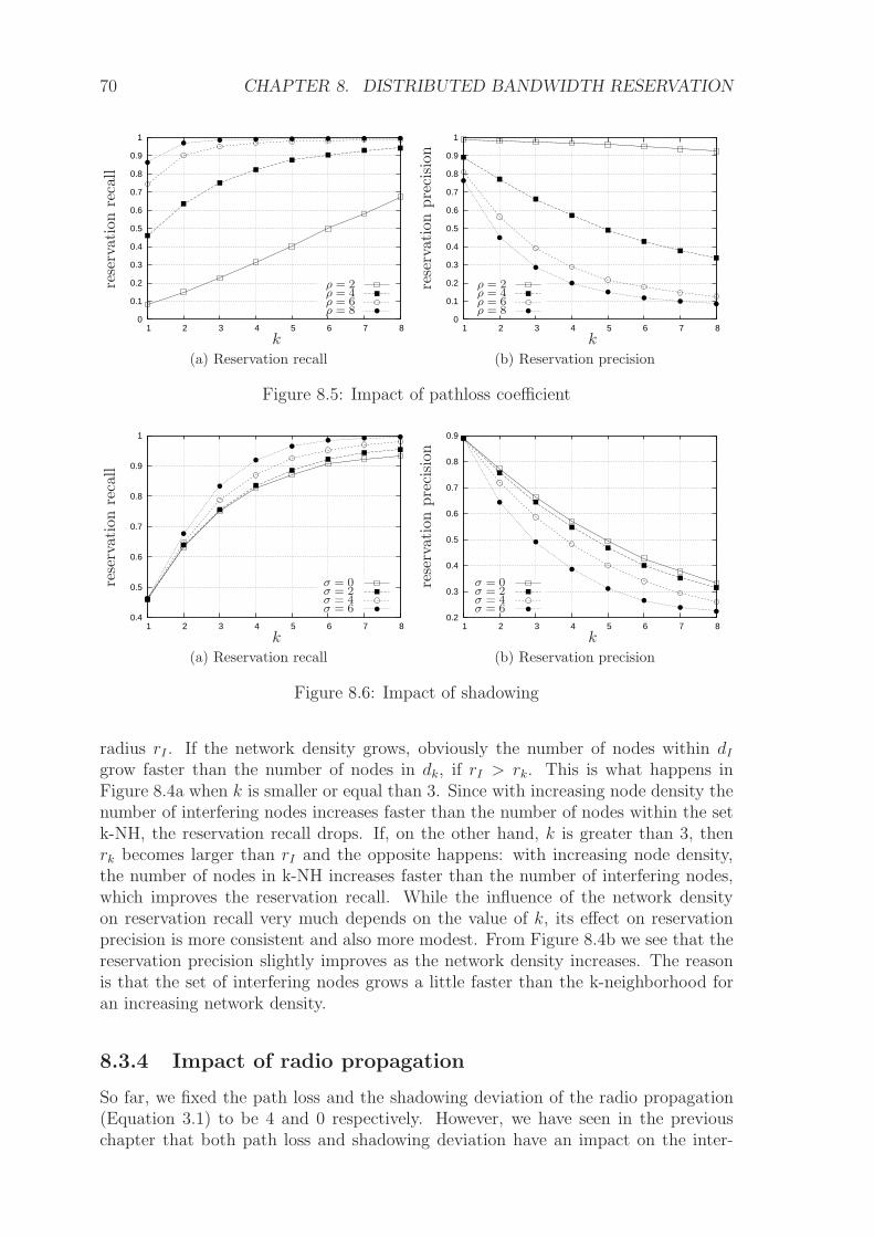
70 CHAPTER 8. DISTRIBUTED BANDWIDTH RESERVATION
0
0.1
0.2
0.3
0.4
0.5
0.6
0.7
0.8
0.9
1
1 2 3 4 5 6 7 8
ρ = 2ρ = 4ρ = 6ρ = 8
rese
rvat
ion
reca
ll
k(a) Reservation recall
0
0.1
0.2
0.3
0.4
0.5
0.6
0.7
0.8
0.9
1
1 2 3 4 5 6 7 8
ρ = 2ρ = 4ρ = 6ρ = 8
rese
rvat
ion
pre
cisi
on
k(b) Reservation precision
Figure 8.5: Impact of pathloss coefficient
0.4
0.5
0.6
0.7
0.8
0.9
1
1 2 3 4 5 6 7 8
σ = 0σ = 2σ = 4σ = 6
rese
rvat
ion
reca
ll
k(a) Reservation recall
0.2
0.3
0.4
0.5
0.6
0.7
0.8
0.9
1 2 3 4 5 6 7 8
σ = 0σ = 2σ = 4σ = 6
rese
rvat
ion
pre
cisi
on
k(b) Reservation precision
Figure 8.6: Impact of shadowing
radius rI . If the network density grows, obviously the number of nodes within dIgrow faster than the number of nodes in dk, if rI > rk. This is what happens inFigure 8.4a when k is smaller or equal than 3. Since with increasing node density thenumber of interfering nodes increases faster than the number of nodes within the setk-NH, the reservation recall drops. If, on the other hand, k is greater than 3, thenrk becomes larger than rI and the opposite happens: with increasing node density,the number of nodes in k-NH increases faster than the number of interfering nodes,which improves the reservation recall. While the influence of the network densityon reservation recall very much depends on the value of k, its effect on reservationprecision is more consistent and also more modest. From Figure 8.4b we see that thereservation precision slightly improves as the network density increases. The reasonis that the set of interfering nodes grows a little faster than the k-neighborhood foran increasing network density.
8.3.4 Impact of radio propagation
So far, we fixed the path loss and the shadowing deviation of the radio propagation(Equation 3.1) to be 4 and 0 respectively. However, we have seen in the previouschapter that both path loss and shadowing deviation have an impact on the inter-

8.4. END-TO-END RESERVATIONS 71
ference perceived at a given node. Figure 8.5 illustrate the effect of the path losscoefficient on recall and precision. It is shown that the bigger the path loss coeffi-cient, the higher the recall (at the expense of a lower precision). The reason is that ahigh path loss coefficient makes the signal drop below the interference threshold veryquickly and thus makes the set of interfering nodes approach the 1-hop neighborhood.That’s why – already for a k of 1 – the recall for a path loss coefficient of 8 becomesbigger than 0.8. On the other hand, the precision drops very quickly for high pathloss values (Figure 8.5b). This is because most nodes outside the 1-hop neighborhoodno longer.
Figure 8.6a shows how reservation recall evolves when the radio propagation be-comes irregular. From the Figure, we observe that for a given value of k, the reserva-tion recall improves as σ increases. The reason is, as mentioned in chapters 4 and 7,the increasing σ in the LNS model also increases the transmission range of the node.It follows that the set of decoders Dn increases and so does the set of of k-neighbors,which improves the overall reservation recall. How the reservation precision is af-fected by irregular radio propagation is illustrated in Figure 8.6b. It can be observedthat the reservation precision drops as σ increases. This is what we would expectsince the higher the values for σ the more randomness is induced into the signal. Asthe randomness increases, the correlation between the number of hops of a sourcedestination pair and its Euclidean distance is reduced.
8.4 End-to-end reservations
Reservation recall and precision give an indication of the quality of a reservation forone single transmission. In practice, one is interested in the quality of a reservationof a whole flow.Bandwidth and throughput capacity are concave metrics. The throughput of a flowis determined by the lowest bandwidth available along the flow. Similarly, the qualityof a flow is determined by the lowest reservation recall along the path. We thereforedefine a new metric, the so called reservation quality Qk
n′ ,nfor a flow with node n
′
being the source node and node n being the destination node:
Qkn′,n
= min(n′′′ ,n′′)∈η(n′ ,n)
Rkn′′←n′′′ (8.5)
As with reservation recall and precision for a single transmission, we also want toconsider the downside of a high quality reservation, namely the amount of resourceswasted along the path from node n to node n
′. This is reflected by the so called
reservation loss Lkn′ ,n
Lkn′ ,n
=
∑
(n′′′ ,n′′)∈η(n′ ,n) | k-NHn′′ ∩ In′′←n′′′ |∑
(n′′′ ,n′′)∈η(n′ ,n) | k-NHn′′ | . (8.6)
Obviously, if | η(n′, n) |= 1, both the reservation quality and reservation loss are
identical to reservation recall and precision respectively. As with capacity (Equation5.13), reservation quality and loss are defined over a traffic pattern Υ (Equation 5.9).Thus, for a given set of flows Υ, 1
k·|Υ|∑k−1
i=0
∑
(n′ ,n)∈ΥQkn′ ,n|X=xi is an approximation

72 CHAPTER 8. DISTRIBUTED BANDWIDTH RESERVATION
0
0.1
0.2
0.3
0.4
0.5
0.6
0.7
0.8
0.9
1
2 4 6 8 10 12 14 16 18 20
rese
rvat
ion
qual
ity
path length
ρ = 2ρ = 4ρ = 6ρ = 8
(a) Reservation quality
0
0.2
0.4
0.6
0.8
1
2 4 6 8 10 12 14 16 18 20
rese
rvat
ion
loss
path length
ρ = 2ρ = 4ρ = 6ρ = 8
(b) Reservation loss
Figure 8.7: Reservation quality and loss vs path length
for the expected reservation quality of a network. Similarly, 1k·|Υ|
∑k−1i=0
∑
(n′ ,n)∈Υ Lkn′ ,n|X=xi
is an approximation for the expected loss of a network.
8.5 Reservation quality and Loss in random net-
works
We consider uniform random network topologies of 200 nodes being deployed in anarea of 2000m× 2000m and we use the very same settings for interference, transmis-sion power, routing and scope as in section 8.3. Now, we are interested in how thereservation quality Qk and loss Lk behave as the length of the path increases.
8.5.1 Trade-off between reservation quality and loss
Figure 8.7 shows both Qk and loss Lk as a function of the path hop length | η(n, n′) |
for k = 2 and for different pathloss values ρ. A first observation is that, for areasonably long path, the reservation quality is beyond repair. The result tells us thatthere is a high probability that a reservation along the path covers only about 20%of all interfering nodes. As expected, increasing ρ improves the reservation quality atthe expense of the reservation loss. Similar to reservation recall and precision, thereis a trade-off between reservation quality Qk and reservation loss Lk (Figure 8.7b).The Figure also shows that if the path length increases, the curves start to resemble alinear function. This implies that if the path is long enough, any change in ρ equallyaffects Qk and Lk. There is one notable distinction in the behavior of reservationquality Qk and loss Lk in Figure 8.7. While reservation loss converges very quickly,the reservation quality keeps dropping with increasing path length, particularly for aρ of 8 or 6. This is due to the concave property of the Qk metric which defines thereservation quality as the minimum reservation recall along the path.
8.5.2 Effects of fading
Figure 8.8 illustrates the effect of fading on reservation quality and loss for k = 2.In section 8.3 we mentioned that shadowing increases the average signal power per

8.6. SUMMARY 73
0.1
0.2
0.3
0.4
0.5
0.6
0.7
1 2 3 4 5 6 7 8 9 10
rese
rvat
ion
qual
ity
path length
σ = 0σ = 2σ = 4σ = 6
(a) Reservation quality
0
0.2
0.4
0.6
0.8
1
1 2 3 4 5 6 7 8 9 10
rese
rvat
ion
loss
path length
σ = 2σ = 2
σ = 4σ = 6
(b) Reservation loss
0
5
10
15
20
25
30
35
5 10 15 20 25 30 35
P
|k-N
H∩
I|
P
| k-NH |
(c) Correlation between∑ | k-NH | and
∑ |k-NH ∩ I | for σ = 6
0
5
10
15
20
25
30
35
40
45
50
10 15 20 25 30 35 40 45 50 55 60
P
|k-N
H∩
I|
P
| k-NH |
(d) Correlation between∑ | k-NH | and
∑ |k-NH ∩ I | for σ = 6
Figure 8.8: Reservation quality and loss
distance and therefore augments the set of direct neighbors Dn of a node n. Thishas an augmenting effect on reservation recall and, as a consequence, also increasesthe reservation quality of a flow (Figure 8.8a). The reservation loss L on the otherhand, decreases with increasing values of σ, similar to reservation precision (Figure8.8b). A look at the definition of reservation loss (Equation 8.6) explains what hap-pens. Reservation loss relates the sum of all interfering k-neighbors to the sum ofk-neighbors along the path. Figures 8.8c-d show the correlation between these twocomponents for k = 2 and different values of σ. No loss at all would require the sumof interfering k-neighbors to match the sum of k-neighbors. In such a case, the cor-relation plot would look like a straight line with a slope of one. From Figures 8.8c-dwe see that with increasing values of σ, the correlation plot progressively shifts froma line-like shape to a cloud. The cloud in Figure 8.8d emerges if there is no realcorrelation between the sum of interfering k-neighbors and the sum of k-neighbors,which obviously is the case as σ grows.
8.6 Summary
In this chapter we studied the bandwidth reservation in ad hoc networks. To do so, wehave defined to two metrics of interest: Reservation recall which models the quality ofa reservation. And reservation precision which models the amount of resources that
74 CHAPTER 8. DISTRIBUTED BANDWIDTH RESERVATION
are wasted due to a reservation. We have shown that there exists a clear trade-offbetween reservation recall and precision since optimizing recall is done at the cost ofprecision. This is because there is no exact correlation between the k-neighborhoodand the set of interferer for a given transmission. A large k-neighborhood increases theinterference coverage but induces over-reservation. In the chapter, we have also shownthat irregular radio propagation diminishes the reservation precision but improves therecall. One reason for this is that the set of nodes in a k-neighborhood grows underfading, which then increases the interference coverage. Recall and precision have adirect impact on the quality of a bandwidth reservation along the path of a flow. Wehave shown that even for a 3-hop wide reservation, there is a high probability thata reservation along the path covers only about 20% of all interfering nodes. In thiswork, we considered only static networks. One could imagine that the situationdeteriorates even more in mobile scenarios, where nodes occupying a reservationleave the interfering area at some point in time. The conclusion is that distributedbandwidth reservations are inadequate to provide QoS in MANETs and that othertechniques have to be considered, e.g., priority based approaches.

Part II
System

Chapter 9
The invisible ad hoc network
After having discussed some of the more formal and theoretical problems of ad hocnetworks in part I of this dissertation, we want in this part to look at ad hoc net-works from a systems perspective. In chapter 1 we have described some of the possibleapplication scenarios of ad hoc networks. Unfortunately, up to now, only a few realdeployments of ad hoc networks exist, and most of them are at Universities or researchlaboratories. One reason for this is that there are not enough suitable applicationsavailable for ad hoc networks. In order for certain applications to run in MANETsthey have to be able to cope with the complexity of the underlying ad hoc network,be it the error prone wireless media or the lack of infrastructure and central compo-nents. In an effort to overcome the absence of practical applications for MANETs,researchers have designed and implemented several dedicated applications that weretailored towards the requirements of MANETs. Those applications particularly takethe very specific properties of MANETs into account, but at the same time, theirusage is restricted to MANETs only, which prohibits access to a broader audience.In practice, users prefer to use the same application regardless of the network they arecurrently part of. We believe that, rather than building dedicated applications, oneshould provide a network infrastructure to allow existing applications to run seam-lessly in ad hoc networks. In order to implement this goal, we present in this partof the dissertation, network abstractions and services that hide the complexity of theunderlying ad hoc network to higher software layers. Our approach can be seen asan effort to turn MANETs into an invisible network to open access for traditionalInternet based applications.
In the first chapter of this part of the thesis we present the design and implemen-tion of a virtual interface that allows nodes running different media access technologiesto form one single ad hoc network. Thereby, the virtual interface is hiding all theheterogeneity of the different wireless media access technologies below a standard IPinterface. We evaluate our approach in terms of throughput and handover-time usingIEEE 802.11 and Bluetooth as two examples of wireless access technologies.
In the remainder of this thesis, we present the architecture of several fundamentalnetwork services for MANETs. Many distributed applications that potentially wouldsuit for MANETs expect certain services like DNS or SIP to run. However, theinherent distributed and infrastructure-less nature of MANETs has highlighted howfundamental services, such as DNS, SIP, SLP, etc., rely on a centralized client-servermodel. The absence of those basic services in MANETs does not strictly preventnetworking, but it strongly restraints the adoption of ad hoc networks as a plug-and-

78 CHAPTER 9. THE INVISIBLE AD HOC NETWORK
play technology. Ideally, traditional Internet-based applications would run seamlesslyin ad hoc networks, without the need for any change re-configuration. One approachto achieve this goal is to provide distributed versions of network services in MANETs,while still maintaining the standardized interface of those services.
Recently, there have been many different attempts at implementing network ser-vices in MANETs using a variety of technologies including, e.g., extensions to routingprotocols [75] and distributed hash tables (DHTs) [76, 77, 78, 79]. In practice, mostof these solutions are either not efficient enough or they introduce severe limitationson how the MANET can be operated. For instance, some solutions only work on aparticular routing protocol [75], other solutions require a fixed node to be stable andavailable at all times [76, 79], and yet a third set of solutions treat MANETS likethe Internet and try to build overlay networks that end up being too expensive tomaintain [78, 79].
In this thesis, we take a radically different approach to the problem. We first focuson the fundamental infrastructure needed to implement a basic directory service onMANETs. Briefly explained, sharing information in MANET can be seen as theproblem of dynamically storing and performing lookups over key/value pairs. Wehave developed and implemented a system called MAND which provides mechanismsto store and lookup tuples (key/value pairs) over a MANET. MAND exploits the factthat MANET routing protocols periodically exchange information using a variety ofrouting messages. Given that finding a service or a particular piece of informationin a MANET requires to establish a route to wherever the service is located, MANDpiggybacks the message traffic required to spread information across the MANETon the routing messages, thereby requiring no additional traffic. At the same time,MAND does not impose any constraints on the type of routing protocol that is usedin the network, nor does it require the routing protocol to be modified or re-compiled.
We use the MAND directory service to build more complex services with broadersemantics. In chapter 12 we present a fully decentralized and SLP compatible ser-vice discovery infrastructure for MANETs. We also show how such a system can beused to implement an efficient MANET-Internet gateway solution. In chapter 13, wepresent DOPS (Domain Name and Presence Service for Ad Hoc Networks), a middle-ware platform for domain name resolution in MANETs which also provides seamlessinteraction with the Internet. In chapter 14, we describe SIPHoc, a middleware plat-form for session establishment and management in MANETs. To demonstrate thepotential of SIPHoc and its feasibility, we have used SIPHoc to provide a VoIP solu-tion that supports VoIP conversations within a MANET and between the MANETand end-points on the Internet. In chapter 16 we present an application for socialnetworking in ad hoc networks.
The design and implementation of all the services presented in this thesis is tai-lored to MANETs of a reasonable size of up to 100 nodes at maximum. The foun-dation of this assumption lies in part I of this thesis where we have shown howthroughput capacity scales with the network size. We believe that throughput ca-pacity is the major limiting factor that dermines to what size ad hoc network willscale.
To emphasize the practical relevance of our work, we have implemented all theservices proposed in this thesis in Linux. Our deployment testbed consists of 23Linux driven Nokia N800 handheld devices. Experiments have been done to studythe reliability and the performance of the systems.
Chapter 10
Heterogeneous Mobile Ad HocNetworks
Ad Hoc Networks are considered to be formed spontaneously between various differ-ent wireless devices. The devices participating an ad hoc network may vary in termsof CPU performance, memory capacity or bandwidth. In some cases, the devicesmay even be equipped with different media access technologies. Current media ac-cess proposals for wireless networks range from Bluetooth [80] and IEEE 802.15.4 [81]up to 802.11 [82]. Already within the 802.11 group there exist many different flavors(802.11e/g/b/a/h). Nevertheless, most research on MANETs assumes such networksto have one common MAC schema. In this chapter, we discuss the integration ofheterogeneous mobile ad hoc networks comprising different MAC protocols. We de-scribe and discuss the performance of an end-to-end communication abstraction thattransparently hides the heterogeneity of the underlying medium access schema whilestill supporting node mobility, multi-hop transmission, simple addressing, etc. Sucha heterogeneous mobile ad hoc networks occurs, e.g., when combining a BluetoothPAN with an 802.11 MANET as shown in Figure 10.1. An example is a universitycampus with all sorts of personal devices ranging from mobile phones, handhelds upto laptops. Each of these devices may be equipped with different communicationtechnologies tailored to their capabilities and intended use. Bluetooth, e.g., is anenergy-saving technology commonly used in mobile phones or handhelds. Laptops onthe other hand do not have such strong constraints, they might include an 802.11 aswell as a Bluetooth interface. Ubiquitously combining all these devices into one het-erogeneous mobile ad hoc network could invite new application and services like, e.g.,location based services or VoIP. In such scenarios, a personal device of one particu-lar PAN might communicate with a personal device of another PAN in a multi-hopfashion where the underlying MAC scheme changes on a per hop basis. Anotherinteresting application of a heterogeneous mobile ad hoc network is the integrationof various personal devices into a so called digital home. In a digital home, PCs andconsumer electronics could work together on an ad hoc basis to different rooms inthe house using a combination of networks.
The rest of this chapter is organized as follows. The next section explores vari-ous approaches to build heterogeneous mobile ad hoc networks using Bluetooth and802.11. Section 10.3 presents our solution which is based on virtual layer two device.In section 10.4 we evaluate the system and section 10.7 summarizes the chapter.
79
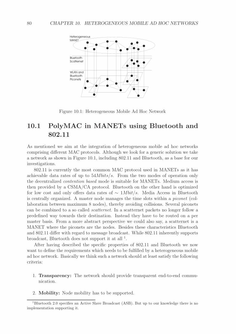
80 CHAPTER 10. HETEROGENEOUS MOBILE AD HOC NETWORKS
Heterogeneous
MANET
Bluetooth
Scatternet
WLAN and
Bluetooth
Piconets
Figure 10.1: Heterogeneous Mobile Ad Hoc Network
10.1 PolyMAC in MANETs using Bluetooth and
802.11
As mentioned we aim at the integration of heterogeneous mobile ad hoc networkscomprising different MAC protocols. Although we look for a generic solution we takea network as shown in Figure 10.1, including 802.11 and Bluetooth, as a base for ourinvestigations.
802.11 is currently the most common MAC protocol used in MANETs as it hasachievable data rates of up to 54Mbits/s. From the two modes of operation onlythe decentralized contention based mode is suitable for MANETs. Medium access isthen provided by a CSMA/CA protocol. Bluetooth on the other hand is optimizedfor low cost and only offers data rates of ∼ 1Mbit/s. Media Access in Bluetoothis centrally organized. A master node manages the time slots within a piconet (col-laboration between maximum 8 nodes), thereby avoiding collisions. Several piconetscan be combined to a so called scatternet. In a scatternet packets no longer follow apredefined way towards their destination. Instead they have to be routed on a permaster basis. From a more abstract perspective we could also say, a scatternet is aMANET where the piconets are the nodes. Besides these characteristics Bluetoothand 802.11 differ with regard to message broadcast. While 802.11 inherently supportsbroadcast, Bluetooth does not support it at all 1.
After having described the specific properties of 802.11 and Bluetooth we nowwant to define the requirements which needs to be fulfilled by a heterogeneous mobilead hoc network. Basically we think such a network should at least satisfy the followingcriteria:
1. Transparency: The network should provide transparent end-to-end commu-nication.
2. Mobility: Node mobility has to be supported.
1Bluetooth 2.0 specifies an Active Slave Broadcast (ASB). But up to our knowledge there is noimplementation supporting it.

10.2. OVERVIEW 81
Application
Transport
IP
MAC
802.11 Device
IP Interface
Connection
based
Bluetooth
Device
Figure 10.2: Communication Abstraction: (a) Transport Layer (b) Application Layer(c) IP Layer
3. Addressing: Addressing should be independent of how many interfaces areattached to a particular node.
4. Configuration: Configuring a node should be possible without any knowledgeof the underlying MAC technology.
In a nutshell, what we are looking for is an end-to-end communication abstractionthat supports MAC-switching2, node mobility and multi-homing 3. Certainly twoissues to be solved are broadcast emulation and handover. Broadcast emulation sinceit is not directly supported in Bluetooth (nor on nodes comprising both Bluetoothand 802.11). Handover since in the case of heterogeneous mobile ad hoc networks ahandover might include a change in how the medium is accessed. A handover canbe caused by node mobility, a change in user preferences (the user chooses to saveenergy and use Bluetooth instead of 802.11), or performance reasons. We will cometo that point later in section 10.3.
10.2 Overview
In principle, a communication abstraction like the one proposed in the previoussection can be provided on any layer above MAC. SCTP [83], or Stream ControlTransmission Protocol, is a transport protocol defined by the IETF providing similarservices to TCP. It ensures reliable, in-sequence transport of messages. While TCPis byte-oriented, SCTP deals with framed messages. A major contribution of SCTPis its multi-homing support. One (or both) endpoints of a connection can consist ofmore than one IP addresses, enabling transparent fail-over between hosts or networkcards. Since both, 802.11 and Bluetooth have IP bindings, one could think of usinga common MANET routing protocol. Each interface could be separately configuredand maintained (AODV-UU [84], e.g., supports multiple interfaces). This solution(see Figure 10.2a) seems to be quite promising in terms of performance since SCTPoptimizes the transmission over multiple links. In fact, if one particular node can bereached through several interfaces, SCTP switches transmission from one interfaceto another after a predefined number of missing acknowledgements. Unfortunately,the solution lacks transparency. Applications running traditional Unix sockets wouldhave to be changed to use SCTP sockets instead. Another problem arises with theconnection oriented nature of Bluetooth. In Bluetooth, interfaces appear and dis-appear dynamically depending on whether the connection to the specific node iscurrently up or down. Therefore, this is something that both the ad hoc routing
2Refers to the fact that the used MAC technology may change along a source/destination path3A node having multiple network interfaces

82 CHAPTER 10. HETEROGENEOUS MOBILE AD HOC NETWORKS
protocol as well as SCTP would have to cope with. Recently, the Network WorkingGroup at the IETF proposed ASCONF [85], a feature that allows dynamic recon-figuration of IP addresses during an SCTP session. On the routing layer, however,we are not aware of any protocol that supports dynamic interfaces. Typically, theseprotocols expect the network interfaces to be configured statically within the system.And even if routing modules were able to handle dynamic interfaces, still the map-ping between the nodes and IP addresses would have to be solved. Instead of usingan all-IP communication based on SCTP and a MANET routing protocol, one couldas well think of an application layer solution (see Figure 10.2b). In [86], the authorspropose a communication framework based on JXTA [87, 88] that is in charge oftransporting packets end-to-end by choosing the right transport mechanism below,i.e 802.11/IP or raw Bluetooth. This allows the use of separate optimized routingalgorithms for IP and Bluetooth respectively. Unfortunately, this solution goes atthe expense of performance. How should the application layer framework decidewhich subsystem best to send the packet to without using flooding? Furthermore,application transparency is not given at all. Rather, transparency can be providedwhen multi homing is implemented on a lower layer. Imagine a single IP interface(virtual interface) handling different physical interfaces (see Figure 10.2c). Neitherthe application nor the routing would be affected by the fact that eventually a nodeconsists of multiple interfaces belonging to different MAC technologies. But how cansuch an interface know about the real physical interface to send the packet to? Howfeasible is such a solution? The following sections not only shows that such a solutionis feasible, but also that it performs well.
10.3 A MAC Layer Approach
As discussed, a virtual interface approach is the most convenient solution for hetero-geneous mobile ad hoc networks in terms of transparency. The question now is howto implement it and how to make it perform well.
10.3.1 Linux Ethernet Bridge
The solution we propose here is inspired by the Linux Ethernet bridge [89, 90]. Sim-ilar to a physical bridge device, the Linux Ethernet bridge ties separate layer-two-networks together, only that it is purely software. The bridge includes much of thefunctionality we would like to see in a virtual interface as described at the end of sec-tion 10.1. Appearing to the operating system as a regular layer-two-device one caneasily assign IP addresses to bridges. The bridge is supposed to work in combinationwith 802.x devices, therefore not including Bluetooth. Fortunately, the Bluetoothpersonal area network (PAN) profile specifies BNEP [91] which itself defines a packetformat to transport common networking protocols over the Bluetooth media. BNEPsupports the same networking protocols that are supported by IEEE 802.3/Ethernetencapsulation, therefore enabling Bluetooth to be used within the bridge. Layer-two-bridges have the well known property of forwarding packets to the correct physicalnetwork corresponding to the destination MAC address. So the bridge’s decision fora frame is one of these:
• bridge it, if the destination MAC address is on another side of the bridge

10.3. A MAC LAYER APPROACH 83
MAC
IP
Transport
AODV
Application
Virtual
Interface vi
Broadcast Unicast
NDBPrioritiesTimer
HCI
L2CAP
HC
ID
SDPD
BN
EP
802.x Interface
Figure 10.3: Virtual Interface Approach
A
B
C
A
B
C
Priorities NbdB->eth1, bnep0
C->bnep0
Bnep0 -> 7
Eth1-> 1
Bnep0 -> 7
Eth1-> 1
Bnep0 -> 1
A->eth1, bnep0
C->bnep0
A->bnep0
B->bnep0
Figure 10.4: The Neighborhood Database (NDB)
• flood it over all the forwarding bridge ports, if the position of the box with thedestination MAC is unknown to the bridge
• pass it to the higher protocol code (IP) if the destination MAC address is thatof the bridge or of one of its ports
• ignore it if the destination MAC address is located on the same side of thebridge
As the bridge learns about the neighboring nodes and their MAC addresses, itis capable of forwarding the packet to the right physical interface instead of justflooding the packet. It does so by keeping a neighborhood database (NDB) mappingdestination MAC addresses to physical interfaces. Entries are refreshed by incomingpackets, otherwise they time out.
10.3.2 The virtual Interface
Since we are looking for a virtual interface, we are not interested in packet for-warding, but the idea of storing a MAC/interface mapping based on incoming packetsis also suitable for local traffic. We have implemented a virtual interface (vi) thatadopts this mechanism. Like the Linux Ethernet bridge, the vi represents a regularlayer-two-device and can be configured accordingly. The vi allows to plug in any802.x compatible network device, like e.g a wireless LAN card or a BNEP/Bluetoothconnection, while hiding the heterogeneity of the used devices from the upper layers.For every neighboring node, the vi holds an array of possible outgoing interfaces.The number of entries in the array follows directly from the intersection of the twosets of interfaces. An entry contains a time-stamp and is created upon receivingthe first packet (i.e a routing broadcast message or a route reply) of the associatedneighbor/interface pair. Every consecutive incoming packet refreshes the time-stamp.

84 CHAPTER 10. HETEROGENEOUS MOBILE AD HOC NETWORKS
Algorithm 10.1 Local packet processing
1: receiving packet(vi, p);2: if p.type = BROADCAST then3: interfaces := get interfaces(vi);4: for all i in interfaces do5: transmit(i, p);6: end for7: else8: current := ndb[hashval(p.mac.dst address)];9: outgoing := NULL;
10: while current 6= NULL do11: if outgoing = NULL then12: outgoing := current;13: else if current.priority < outgoing.priority then14: ∆ := outgoing.ts - current.ts;15: if ∆ < vi.maxdiff then16: outgoing := current;17: end if18: else19: ∆ := current.ts - outgoing.ts;20: if ∆ > vi.maxdiff then21: outgoing := current;22: end if23: end if24: current := current.next;25: end while26: if outgoing 6= NULL then27: transmit(outgoing, p);28: end if29: end if
The processing of outgoing packets is done using Algorithm 10.1. If the vi receivesa packet from the upper layer for delivery, it first checks the packet type (line 2,Alg. 10.1). In case the packet is a broadcast packet, it will be sent through allavailable interfaces (lines 4-6, Alg. 10.1). Therefore, the vi also acts as a broadcastemulation layer for Bluetooth. This is particularly important since BNEP is point-to-point. However, if the packet is unicast (lines 7-29, Alg. 10.1), the vi looks forthe corresponding entry in the neighborhood database (line 8) mentioned above andretrieves the information about the interface the packet has to be sent to (entries areperiodically checked for expiration). If there is more than one option, the vi makesuse of another feature, the so called priority table. The priority table specifies somesort of ranking among the interfaces, meaning that whenever a given neighbor canbe reached through several interfaces, the interface with the lowest priority is taken.Figure 10.3 illustrates the architecture of the virtual interface and how it is embeddedwithin the network stack. The state of the neighborhood database and priority tablein a scenario where three nodes form a neighborhood (they are within transmissionrange of each other) is shown in Figure 10.3.2.
Apart from the priority table, another mechanism is needed to prevent links frombecoming stalled. Imagine two nodes, each of them containing an 802.11 as well asa Bluetooth interface. Obviously, there are two ways for the two nodes to exchangepackets, therefore the corresponding neighborhood database contains two entries.Further, assume the Bluetooth interface to have the highest priority on the sender
10.3. A MAC LAYER APPROACH 85
node (the node might be battery driven and tries to minimize energy consumptionper packet transmission). If the Bluetooth connection temporarily suffers from verybad link properties, the node probably wants to switch to the 802.11 interface at theexpense of a higher energy consumption. This will not be possible under the currentsetup as the vi always uses the interface with the highest priority to transmit thepacket. To overcome this unfavorable situation, a cleanup timer, which periodicallyremoves all expired entries, could be used (an entry is expired if it has not beenrefreshed for a certain amount of time), but this would unnecessarily increase routingtraffic since the next packet in the queue right after the cleanup is triggering a routerequest. Instead of a cleanup timer, we therefore use a different mechanism that issort of routing-friendly. We introduce a new parameter that is associated with a vi,the so called maxdiff threshold. The maxdiff threshold unit is 10ms and it decideshow much two single entries within the neighborhood database may differ in terms oftime-stamps to keep the priority policy up. So a higher ranked interface entry can bereplaced by a lower priority interface if the time-stamp differs for more than maxdiff(line 15, line 20, Alg. 10.1).
10.3.3 Configuration
The virtual interface consists of a kernel module and a user-mode command-line tool 4.The kernel module immediately gets loaded when creating a new virtual interfaceusing the victl addvi command. There are also commands to add and remove devicesto/from the virtual interface as well as to set the interface priorities. Table 10.1shows how a virtual interface containing Bluetooth and WLAN is typically set up.Like a regular layer-two-interface, the IP configuration of vi can be performed withifconfig. The question that remains is how to dynamically add Bluetooth devicesto the vi (remember that they appear on a connection basis). Apparently, we needsome help from Bluez [92] here. A script is called whenever a Bluetooth interfaceis created. We then simply let the vi maintenance be triggered by this event, asshown in Figure 10.2. Devices are added and removed to/from the vi every time theyappear or disappear. Another issue to take care of is the MAC address of the vi.The MAC address can manually be set using the victl addr command. This addresscan be totally virtual or correspond to a physical interface. Outgoing packets alwaysadopt the MAC address of the vi, regardless of the interface they leave. Some wirelessNICs do not allow MAC addresses to be overwritten, so the address for the vi is bestchosen to correspond to the address of NIC that cannot be changed. On the contraryin a vi comprising Bluetooth interfaces only, a virtual MAC address is more suitablesince otherwise, communicating nodes would have to adapt their ARP binding everytime the MAC address changes.
10.3.4 Handover
A handover includes route changes as well as MAC switching. In principle, there arethree possible scenarios (see also Figure 10.5):
4Furthermore a C API is provided for the case where the application directly wants interact withthe vi.
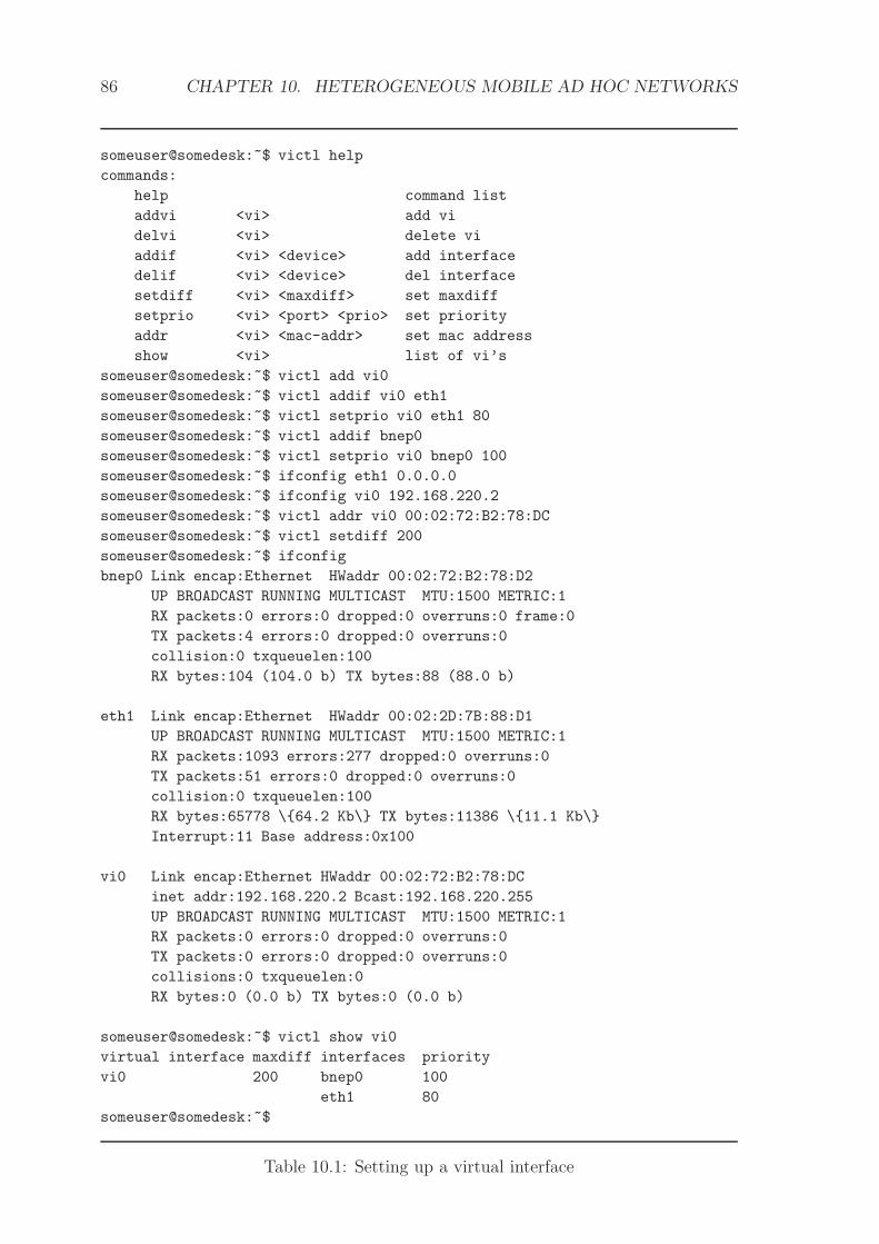
86 CHAPTER 10. HETEROGENEOUS MOBILE AD HOC NETWORKS
someuser@somedesk:~$ victl help
commands:
help command list
addvi <vi> add vi
delvi <vi> delete vi
addif <vi> <device> add interface
delif <vi> <device> del interface
setdiff <vi> <maxdiff> set maxdiff
setprio <vi> <port> <prio> set priority
addr <vi> <mac-addr> set mac address
show <vi> list of vi’s
someuser@somedesk:~$ victl add vi0
someuser@somedesk:~$ victl addif vi0 eth1
someuser@somedesk:~$ victl setprio vi0 eth1 80
someuser@somedesk:~$ victl addif bnep0
someuser@somedesk:~$ victl setprio vi0 bnep0 100
someuser@somedesk:~$ ifconfig eth1 0.0.0.0
someuser@somedesk:~$ ifconfig vi0 192.168.220.2
someuser@somedesk:~$ victl addr vi0 00:02:72:B2:78:DC
someuser@somedesk:~$ victl setdiff 200
someuser@somedesk:~$ ifconfig
bnep0 Link encap:Ethernet HWaddr 00:02:72:B2:78:D2
UP BROADCAST RUNNING MULTICAST MTU:1500 METRIC:1
RX packets:0 errors:0 dropped:0 overruns:0 frame:0
TX packets:4 errors:0 dropped:0 overruns:0
collision:0 txqueuelen:100
RX bytes:104 (104.0 b) TX bytes:88 (88.0 b)
eth1 Link encap:Ethernet HWaddr 00:02:2D:7B:88:D1
UP BROADCAST RUNNING MULTICAST MTU:1500 METRIC:1
RX packets:1093 errors:277 dropped:0 overruns:0
TX packets:51 errors:0 dropped:0 overruns:0
collision:0 txqueuelen:100
RX bytes:65778 \64.2 Kb\ TX bytes:11386 \11.1 Kb\
Interrupt:11 Base address:0x100
vi0 Link encap:Ethernet HWaddr 00:02:72:B2:78:DC
inet addr:192.168.220.2 Bcast:192.168.220.255
UP BROADCAST RUNNING MULTICAST MTU:1500 METRIC:1
RX packets:0 errors:0 dropped:0 overruns:0
TX packets:0 errors:0 dropped:0 overruns:0
collisions:0 txqueuelen:0
RX bytes:0 (0.0 b) TX bytes:0 (0.0 b)
someuser@somedesk:~$ victl show vi0
virtual interface maxdiff interfaces priority
vi0 200 bnep0 100
eth1 80
someuser@somedesk:~$
Table 10.1: Setting up a virtual interface

10.3. A MAC LAYER APPROACH 87
S DS DS D
S
D
Bluetooth
802.11
S Source Node
Destination Node
Broken Link
Node Movement
Figure 10.5: Horizontal (1), Diagonal (2), and Vertical (3) handover
#!/bin/sh
victl addif vi0 \$1
victl setportprio vi0 \$1 80
ifconfig \$1 0.0.0.0
Table 10.2: /etc/bluetooth/pan/dev-up
1. Horizontal Handover: the route changes while the underlying MAC technol-ogy remains the same
2. Vertical Handover: the route does not change but the given neighbor is nowreached through a new physical interface
3. Diagonal Handover: MAC technology and route change simultaneously
Let us now take a closer look at how routes get established in a heterogeneousmobile ad hoc network when using virtual interfaces. In the case of a reactive routingprotocol (e.g. AODV [93]), it is the application that triggers a path setup. Sincethere is no route available yet, the routing protocol typically first broadcasts a routerequest. At the very beginning the neighborhood database contains no entries butthe transmission of a broadcast packet does not need any neighborhood informationanyway (see section 10.3). After the route request has passed several hops, a routereply eventually returns back to the origin. The route reply not only establishes theroute but also creates an entry within the neighborhood database, providing the viwith information on the interface to which the packets to the given neighbor haveto be transmitted. In the case of a pro-active routing protocol (e.g. OLSR [94],things are slightly different. Here nodes periodically broadcast their neighboringinformation and therefore are also creating entries within neighborhood databases.In both cases - proactive and reactive - the NDB entry is established in combinationwith the new route, regardless of whether the MAC technology changes or not. Ina vertical handover on the other hand, the NDB is affected differently. Either thepriority table changes due to user preferences or certain entries expire, meaning theirtimestamp difference exceeds the threshold maxdiff (bad link quality). Obviously,the smaller maxdiff, the more agile the virtual interface is for handover. But a smallmaxdiff threshold can also be unfavorable since it is a counter movement to thepriority policy. If the priorities reflect the bandwidth of the interfaces, then a smallmaxdiff threshold may lead to a diminishing throughput, as we will see in section10.4.
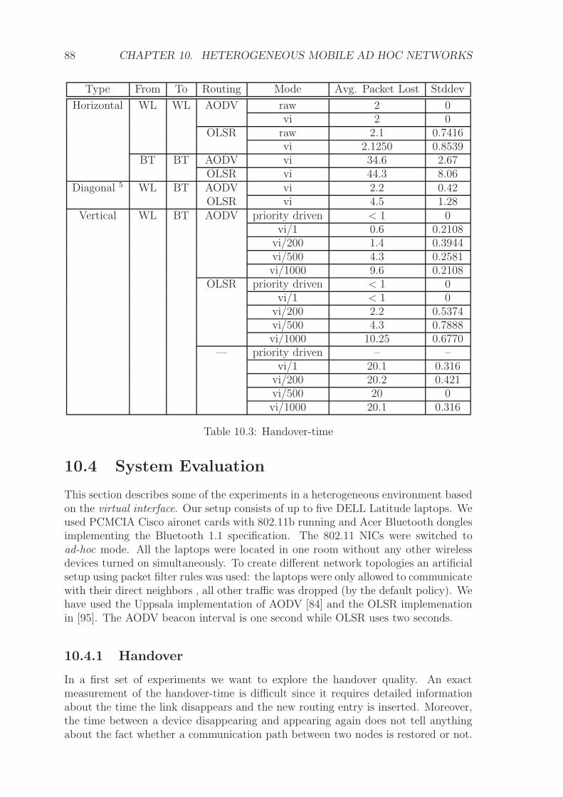
88 CHAPTER 10. HETEROGENEOUS MOBILE AD HOC NETWORKS
Type From To Routing Mode Avg. Packet Lost Stddev
Horizontal WL WL AODV raw 2 0vi 2 0
OLSR raw 2.1 0.7416vi 2.1250 0.8539
BT BT AODV vi 34.6 2.67OLSR vi 44.3 8.06
Diagonal 5 WL BT AODV vi 2.2 0.42OLSR vi 4.5 1.28
Vertical WL BT AODV priority driven < 1 0vi/1 0.6 0.2108
vi/200 1.4 0.3944vi/500 4.3 0.2581vi/1000 9.6 0.2108
OLSR priority driven < 1 0vi/1 < 1 0
vi/200 2.2 0.5374vi/500 4.3 0.7888vi/1000 10.25 0.6770
— priority driven – –vi/1 20.1 0.316
vi/200 20.2 0.421vi/500 20 0vi/1000 20.1 0.316
Table 10.3: Handover-time
10.4 System Evaluation
This section describes some of the experiments in a heterogeneous environment basedon the virtual interface. Our setup consists of up to five DELL Latitude laptops. Weused PCMCIA Cisco aironet cards with 802.11b running and Acer Bluetooth donglesimplementing the Bluetooth 1.1 specification. The 802.11 NICs were switched toad-hoc mode. All the laptops were located in one room without any other wirelessdevices turned on simultaneously. To create different network topologies an artificialsetup using packet filter rules was used: the laptops were only allowed to communicatewith their direct neighbors , all other traffic was dropped (by the default policy). Wehave used the Uppsala implementation of AODV [84] and the OLSR implemenationin [95]. The AODV beacon interval is one second while OLSR uses two seconds.
10.4.1 Handover
In a first set of experiments we want to explore the handover quality. An exactmeasurement of the handover-time is difficult since it requires detailed informationabout the time the link disappears and the new routing entry is inserted. Moreover,the time between a device disappearing and appearing again does not tell anythingabout the fact whether a communication path between two nodes is restored or not.

10.4. SYSTEM EVALUATION 89
Restoring a communication path in an ad hoc network with multiple radios and a virequires a lot more. It requires the vi to switch to the new physical interface and itmay also require the route to be re-established. To measure all those effects we usedthe ping command to measure the lost packets. As ping triggers a packet transmissionevery second and as it is UDP based, there is almost a one-to-one relationship betweenthe lost packets and the handover time. In order to take the impact of the routingmodule on the neighborhood database into account, we measured along three tracks.Once using AODV [96] representing the reactive class, once OLSR [94] as a proactiverouting protocol and once without routing module at all. Measurements representaverage values taken from 10 samples and the standard deviation is shown as well.Throughout the measurements we use raw to describe scenarios not including thevirtual interface. On the contrary we use vi/x to indicate scenarios including thevirtual interface with a maxdiff threshold of x. The results are shown in Table 10.3.Apart from measurements marked as ’priority driven’, the priority table reflects thebandwidth proportions of the associated interfaces, therefore 802.11 always has thehighest priority.
Let us look at the horizontal handover first. We trigger a route change by physi-cally detaching the interface of a node. Under our setup we measured a packet lossof roughly 2 packets when the route changed from one hop to another, regardless ofwhich routing protocol was used and whether a vi was included or not. But notethat OLSR is not as stable as AODV (its standard deviation is higher). This isdue to the fact that proactive routing protocols (like OLSR) do not react to routefailures directly but broadcast their routing information on a fixed schedule instead.This behavior is even amplified in a pure Bluetooth network 6. Here we observe adifference in packet loss between the two protocols of 10 packets (34.6 for AODVand 44.3 for OLSR). This makes sense since OLSR is running with a beacon intervalof 2 seconds, while AODV uses only 1 second. It also explains the higher standarddeviation of OLSR compared with the one of AODV. For the diagonal handover -we assume the Bluetooth connection already being established on the MAC level -a similar picture appears, OLSR is always a little behind AODV while being lessstable. However, changing the route simultaneously with the MAC technology doesnot seem to introduce additional overhead in the AODV case. For the vertical han-dover (no route change, but interface switching only) we now also take the maxdiffthreshold into account since it influences the agility in terms of the handover decision.Furthermore, we introduce priority driven handover. While in all other experimentsa handover is triggered by the environment (in our scenario by physically detachingan interface), priority driven means the interface ranking is changed (using victl set-portpriority) during a ping session. From the results given for AODV and OLSR inTable 10.3 we see that packet loss increases with increasing maxdiff threshold andalmost disappears for priority driven handover. The former is reasonable becausethe bigger the maxdiff value, the more the priority policy gets enforced, and a purepriority driven MAC switching would not lead to any switching at all. The latterapproves our idea of implementing MAC-switching transparent at the lowest layerpossible. We also tested the impact of maxdiff values on priority driven handover.As expected, the smaller maxdiff gets the less stable the handover becomes. However,
6Note that after the route gets broken, a bluetooth inquiry is triggered in order to establish anew connection, which is a quite time consuming process.
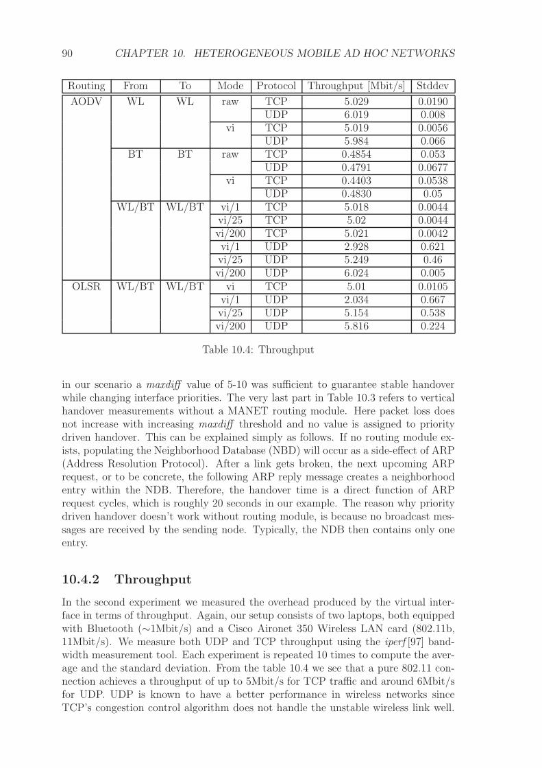
90 CHAPTER 10. HETEROGENEOUS MOBILE AD HOC NETWORKS
Routing From To Mode Protocol Throughput [Mbit/s] Stddev
AODV WL WL raw TCP 5.029 0.0190UDP 6.019 0.008
vi TCP 5.019 0.0056UDP 5.984 0.066
BT BT raw TCP 0.4854 0.053UDP 0.4791 0.0677
vi TCP 0.4403 0.0538UDP 0.4830 0.05
WL/BT WL/BT vi/1 TCP 5.018 0.0044vi/25 TCP 5.02 0.0044vi/200 TCP 5.021 0.0042vi/1 UDP 2.928 0.621vi/25 UDP 5.249 0.46vi/200 UDP 6.024 0.005
OLSR WL/BT WL/BT vi TCP 5.01 0.0105vi/1 UDP 2.034 0.667vi/25 UDP 5.154 0.538vi/200 UDP 5.816 0.224
Table 10.4: Throughput
in our scenario a maxdiff value of 5-10 was sufficient to guarantee stable handoverwhile changing interface priorities. The very last part in Table 10.3 refers to verticalhandover measurements without a MANET routing module. Here packet loss doesnot increase with increasing maxdiff threshold and no value is assigned to prioritydriven handover. This can be explained simply as follows. If no routing module ex-ists, populating the Neighborhood Database (NBD) will occur as a side-effect of ARP(Address Resolution Protocol). After a link gets broken, the next upcoming ARPrequest, or to be concrete, the following ARP reply message creates a neighborhoodentry within the NDB. Therefore, the handover time is a direct function of ARPrequest cycles, which is roughly 20 seconds in our example. The reason why prioritydriven handover doesn’t work without routing module, is because no broadcast mes-sages are received by the sending node. Typically, the NDB then contains only oneentry.
10.4.2 Throughput
In the second experiment we measured the overhead produced by the virtual inter-face in terms of throughput. Again, our setup consists of two laptops, both equippedwith Bluetooth (∼1Mbit/s) and a Cisco Aironet 350 Wireless LAN card (802.11b,11Mbit/s). We measure both UDP and TCP throughput using the iperf [97] band-width measurement tool. Each experiment is repeated 10 times to compute the aver-age and the standard deviation. From the table 10.4 we see that a pure 802.11 con-nection achieves a throughput of up to 5Mbit/s for TCP traffic and around 6Mbit/sfor UDP. UDP is known to have a better performance in wireless networks sinceTCP’s congestion control algorithm does not handle the unstable wireless link well.
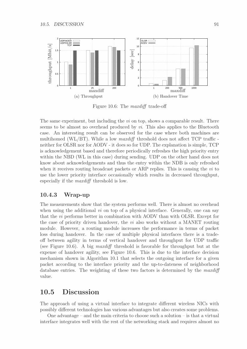
10.5. DISCUSSION 91
0
0.5
1
1.5
2
200251
UDP/AODVUDP/OLSR
TCP
thro
ugh
put
[Mbit/s
]
maxdiff(a) Throughput
0
2
4
6
8
10
12
10005002001
OLSRAODV
del
ay[s
ec]
maxdiff(b) Handover Time
Figure 10.6: The maxdiff trade-off
The same experiment, but including the vi on top, shows a comparable result. Thereseems to be almost no overhead produced by vi. This also applies to the Bluetoothcase. An interesting result can be observed for the case where both machines aremultihomed (WL/BT). While a low maxdiff threshold does not affect TCP traffic -neither for OLSR nor for AODV - it does so for UDP. The explanation is simple, TCPis acknowledgement based and therefore periodically refreshes the high priority entrywithin the NBD (WL in this case) during sending. UDP on the other hand does notknow about acknowledgements and thus the entry within the NDB is only refreshedwhen it receives routing broadcast packets or ARP replies. This is causing the vi touse the lower priority interface occasionally which results in decreased throughput,especially if the maxdiff threshold is low.
10.4.3 Wrap-up
The measurements show that the system performs well. There is almost no overheadwhen using the additional vi on top of a physical interface. Generally, one can saythat the vi performs better in combination with AODV than with OLSR. Except forthe case of priority driven handover, the vi also works without a MANET routingmodule. However, a routing module increases the performance in terms of packetloss during handover. In the case of multiple physical interfaces there is a trade-off between agility in terms of vertical handover and throughput for UDP traffic(see Figure 10.6). A big maxdiff threshold is favorable for throughput but at theexpense of handover agility, see Figure 10.6. This is due to the interface decisionmechanism shown in Algorithm 10.1 that selects the outgoing interface for a givenpacket according to the interface priority and the up-to-dateness of neighborhooddatabase entries. The weighting of these two factors is determined by the maxdiffvalue.
10.5 Discussion
The approach of using a virtual interface to integrate different wireless NICs withpossibly different technologies has various advantages but also creates some problems.
One advantage – and the main criteria to choose such a solution – is that a virtualinterface integrates well with the rest of the networking stack and requires almost no

92 CHAPTER 10. HETEROGENEOUS MOBILE AD HOC NETWORKS
change on the application level. A disadvantage is that not all wireless NICs can beintegrated into a vi that easily. As mentioned, some NICs do not allow for changingtheir MAC address. In principle, there is no problem with this since the neighboringdatabase (NDB) will be able to determine the right outgoing interface for any givendestination MAC address if it has received an incoming packet from the target devicebefore. However, if the MAC address is exclusively associated with a remote NIC,there will only be one entry in the NDB for that given MAC address. In such asituation, Algorithm 10.1 will only have one option where to send a packet to. As aconsequence, priority driven vertical handover will not be possible. Moreover, if thereis no virtual MAC address per node and two nodes have multiple links to choose from(e.g. if both nodes have an 802.11 and a Bluetooth NIC) the ARP cache timeoutdetermines how fast a node will recover from a link outage. One solution would beexplicitely purge the ARP cache more often, but this will harm the performance sincemore ARP requests will be triggered.
10.6 Related Work
There is very little work on network abstractions for different media access tech-nologies in ad hoc networks. In [98, 99], the authors describe the design and imple-mentation of a virtual interface which allows to plug in multiple physical interfaceswith possibly different channel configurations. However, their work does not considermultiple access technologies. Rather they focus on how to efficiently switch to theoptimal channel at a given point in time. VirtualWifi is another approach basedon virtualization [100, 101]. VirtualWifi abstracts a single wireless interface intomultiple virtual interfaces. The basic idea is to switch the physical interface acrossmultiple channels used by each virtual interface. There are other testbed works thatabstract multiple real interfaces into a single virtual interface [102, 103], but againthose approaches do not consider different access technologies.
In [104] the authors present, MR-LQSR, a MANET routing protocol for mult-radio wireless mult-hop networks. MR-LQSR is implemented as a virtual networkadapter, similar to the virtual interface presented in this thesis. The protocol assignsweights to individual links based on the Expected Transmission Time (ETT) of apacket over a link and uses those weights when computing the route for a givenpacket. The difference between MR-LQSR and the vi is that MR-LQSR combinesrouting and multi-radio integration whereas we try to keep those two layers separated.The discussion about cross-layer software is a different one, however, incorporatingmore sophisticated link metrics would certainly be one way to improve the vi. Morework on link metrics to increase the performance of wireless multi-hop networks canbe found in [105]. To some extent, advanced link metrics are orthogonal to Algorithm10.1 since the priorities of each phyisical interface in the vi and the maxdiff valuecan be changed at run-time using victl (see Table 10.1).
There is work on providing seamless access between multiple networks and accesstechnologies in infrastructure-based WLAN networks. The swiss telecommunicationcompany Swisscom developed a device which allows to seamlessly switch betweenWLAN, UMTS and GSM [106]. There are several initiatives to optimize mobility ac-cross heterogeneous networks. The MOBOPTS working group within the IRTF (In-ternet Research Task Force) and the DNA (Detecting Network Attachment) working
10.7. SUMMARY 93
group within the IETF have been investigating ways to support optimized handoverby using appropriate triggers and events from the lower layers. The IEEE 802.21[107] working group is currently working towards a Media Independent Handoverframework in a heteregeneous access environment. Suggestions to improve the han-dover time by taking advantage of IEEE 802.21 are given in [108]. A method usingthe Stream Control Transmission Protocol to facilitate seamless handover betweenwide-area cellular networks such as UMTS and WLAN is presented in [109].
There is also some work on integrating different access technologies in PersonalArea Networks (PANs). ICON [110] offers seamless interoperability accross heteroge-neous access technologies at mobile nodes in PANs. A Distributed Virtual NetworkInterface (DVNI) is proposed in [111] for device discovery, seamless handover androuting in PANs.
10.7 Summary
In this chapter, we have proposed an end-to-end communication abstraction that canbe used in heterogeneous mobile ad hoc networks. Such networks are characterizedby different MAC technologies used among the nodes. The proposed solution is basedon a virtual interface (vi) approach. In this chapter we have shown how the virtualinterface can be used to transparently integrate Bluetooth and 802.11 into one singleIP-based MANET. Note that our solution is not bound to 802.11 or Bluetooth, butworks together with any 802.x-compatible MAC Layer. The vi in combination with aMANET routing protocol supports multihoming, dynamic reconfiguration and nodemobility. The experiments presented demonstrate the feasibility of the abstractionand its potential in building heterogeneous ad-hoc wireless networks.

94 CHAPTER 10. HETEROGENEOUS MOBILE AD HOC NETWORKS
Chapter 11
MAND: Mobile Ad Hoc NetworkDirectory
In chapter 9 we expressed our belief that — in order for MANETs to become ubiqui-tous — MANETs will have to support existing Internet-based applications seamlessly.The problem we target in this chapter is how to implement a simple, efficient platformthat supports standard network services over MANETs. The key observation behindthe solution is that many networking services are based on mapping functionality.For instance, a DNS service maps domain names to IP addresses, or a SIP servicesmaps a SIP URL to a TCP/IP endpoint where the user can currently be accessed.Hence, the focus of this chapter is how to provide an efficient key/value store thatcan be used to implement mapping functions which can then be used to implementbasic network services in MANETs.
11.1 Problem Statement
11.1.1 The design space
A key/value store is a system that provides two basic functions. An insert opera-tion to insert a key/value pair into the system, and a lookup operation to retrieve avalue for a given key. For simplicity, we will use the term tuple as a short name forkey/value pair in the rest of this thesis. In principle, there are three different optionsto implement a distributed key/value store. Either tuples are stored only locally (atthe node that generates the tuple), or they are stored on individual nodes in thenetwork, or they are stored everywhere. We refer to those three approaches as local,hashed and replicated. Any directory service in practice will implement one of thoseapproaches or or a superposition of them. In the following we want to briefly studythe various characteristics of each of those strategies to later motivate the approachwe have taken in this thesis.
Performance: Let us first have a look on the performance of the insert and thelookup operation. In the local strategy insertion will be O(1) and lookup will be O(n),with n being the number of nodes in the network. This is because to look up a tuple,in the worst case it might be necessary to contact every other node in the network.On the other hand, inserting or updating a tuple becomes a local operation. This
95

96 CHAPTER 11. MAND: MOBILE AD HOC NETWORK DIRECTORY
is different with the replicated approach. There, insertion will be O(n) and lookupO(1). In the hashed strategy, the performance of the insert and lookup operationsvery much depend on which node is selected to store the tuple with a given key, andhow fast this node can be discovered and contacted. DHTs – one class of key/valuestores – achieve a performance of O(logn) for both insertion and lookup by storingtuples on nodes that are logically close to the key.
Consistency: Obviously, both the local and the hashed strategy allow nodes toupdate the tuples fast and atomically since there exists only one single instance ofeach tuple. Since network failures are common in MANETs, the hashed approachwill have to be rated slightly worse because updating a tuple requires a connectionto a remote node. A replicated approach, however, may result in a poor consistencyleaving tuples in an inconsistent state. That is either because the distributed updateof all replicas of a tuple cannot be handled atomically, or simply because some nodescannot be reached and therefore their tuples cannot be updated. The latter mayhappen quite frequently in MANETs due routing failures or partial disconnections ofcertain network regions.
Availability: In terms of availability, a replicated strategy performs best. This isbecause even if some nodes turn offline or cannot be reached temporarily, looking upa tuple is still possible due to the replicas available on other nodes. Because of thereplicas, a lookup for a key may even succeed after the originator of the tuple hasalready left the network. In some cases this is not the desired behavior, for instanceif the tuple stored in the network contains information about a service provided bythe originator of the tuple. If on the other hand, a local strategy is used, then theavailability is low because other nodes will not be able to look up a tuple if theycannot contact the originator. This does not pose a problem if the tuple containsinformation about a local service. In this case it is sufficient for a tuple lookup to suc-ceed whenever the service whose contact information is encoded in the tuple can beaccessed. The availability in the hashed strategy is comparable to the one in the localcase. However, again consider the case where tuples hold information about a servicerunning on the node inserting the tuple into the system. Due to network partitionsor routing failures, it may happen that some nodes cannot lookup the tuple includingthe service contact information, even if they could potentially access the service itself.
Memory: Using a local or a hashed strategy requires O(t) memory space, while thememory requirement of a replicated approach is O(t · n), with t being the numberof tuples and n the number of nodes in the network. This makes clear that, a fullreplication of tuples can only be an option in situations where both the number oftuples to be stored and the network size is small.
The various performance aspects of the three different architectures (local, hashedand replicated) are summarized in Table 11.1.
11.1.2 Discussion
Neither of the proposed solutions, local, replicated and hashed, performs well in allmetrics. It is, for instance, impossible to guarantee data consistency and at thesame time provide a fast lookup and high availability, as also stated in the CAP

11.2. SYSTEM MODEL 97
Update Lookup Consistency Availability Memory
Local O(1) O(n) very good bad O(t)Replicated O(n) O(1) bad good O(n · t)Hashed O(logn) O(logn) good very bad O(t)
Table 11.1: Performance vs Consistency vs Availability
theorem [112].In MAND, we provide the user with the flexibility to trade different performance
metrics on a per tuple granularity. Rather than choosing one fixed point in thedesign space, we turn the ability to operate in different modes into a feature ofthe system and a tunable parameter. This is particularly useful when supportingdistributed network services in MANETs. For certain services, a fast response timeis more important than a fast update time. This is the case, e.g., for a DNS service.DNS entries typically remain unchanged, but DNS requests are issued frequently inmodern applications. For other services, it might be important to keep the storedtuples consistent. For instance location based services in ad hoc networks with highmobility. Yet another set of services require that the stored tuples are always fresh.One example is a presence service that allows to query the current online statusof users. MAND provides the flexibility for all those services to operate at theirpreferred point in the design space. Moreover, MAND allows performance trade-offsto be made independently for each tuple that is inserted into the system.
11.2 System Model
The system model of MAND is organized along four design principles:
Fine-grain modes of operation to allow users to choose an optimal trade-off be-tween different metrics such as, e.g., update performance, consistency, avail-ability or lookup performance.
Routing integration to minimize the amount of traffic injected into the network,and to minimize the overall time needed to contact a higher layer service builton MAND.
Layering to guarantee independence of the underlying routing protocol.
Simplicity as the means to provide a robust and efficient software building blockfor implementing higher layer services in MANETs.
11.2.1 Architecture Overview
MAND runs as a user space process on nodes in the ad hoc network (see Figure 11.1)1.It provides two application interfaces, insert(tuple) and lookup(request), that oper-ate on objects of two distinguished datatypes, tuple and request. If not explicitlymentioned we are using the terms tuple and request interchangeably for objects ofthe corresponding type.
1It is not a requirement that all nodes in the network are running an instance of MAND.
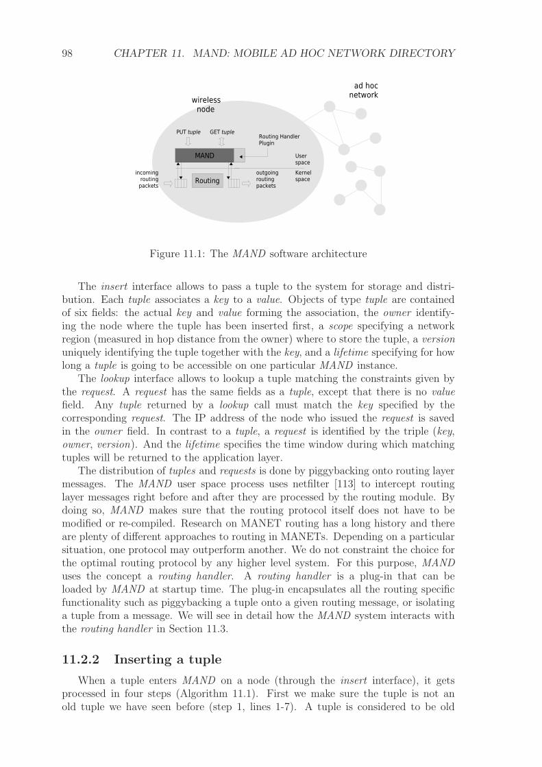
98 CHAPTER 11. MAND: MOBILE AD HOC NETWORK DIRECTORY
Figure 11.1: The MAND software architecture
The insert interface allows to pass a tuple to the system for storage and distri-bution. Each tuple associates a key to a value. Objects of type tuple are containedof six fields: the actual key and value forming the association, the owner identify-ing the node where the tuple has been inserted first, a scope specifying a networkregion (measured in hop distance from the owner) where to store the tuple, a versionuniquely identifying the tuple together with the key, and a lifetime specifying for howlong a tuple is going to be accessible on one particular MAND instance.
The lookup interface allows to lookup a tuple matching the constraints given bythe request. A request has the same fields as a tuple, except that there is no valuefield. Any tuple returned by a lookup call must match the key specified by thecorresponding request. The IP address of the node who issued the request is savedin the owner field. In contrast to a tuple, a request is identified by the triple (key,owner, version). And the lifetime specifies the time window during which matchingtuples will be returned to the application layer.
The distribution of tuples and requests is done by piggybacking onto routing layermessages. The MAND user space process uses netfilter [113] to intercept routinglayer messages right before and after they are processed by the routing module. Bydoing so, MAND makes sure that the routing protocol itself does not have to bemodified or re-compiled. Research on MANET routing has a long history and thereare plenty of different approaches to routing in MANETs. Depending on a particularsituation, one protocol may outperform another. We do not constraint the choice forthe optimal routing protocol by any higher level system. For this purpose, MANDuses the concept a routing handler. A routing handler is a plug-in that can beloaded by MAND at startup time. The plug-in encapsulates all the routing specificfunctionality such as piggybacking a tuple onto a given routing message, or isolatinga tuple from a message. We will see in detail how the MAND system interacts withthe routing handler in Section 11.3.
11.2.2 Inserting a tuple
When a tuple enters MAND on a node (through the insert interface), it getsprocessed in four steps (Algorithm 11.1). First we make sure the tuple is not anold tuple we have seen before (step 1, lines 1-7). A tuple is considered to be old
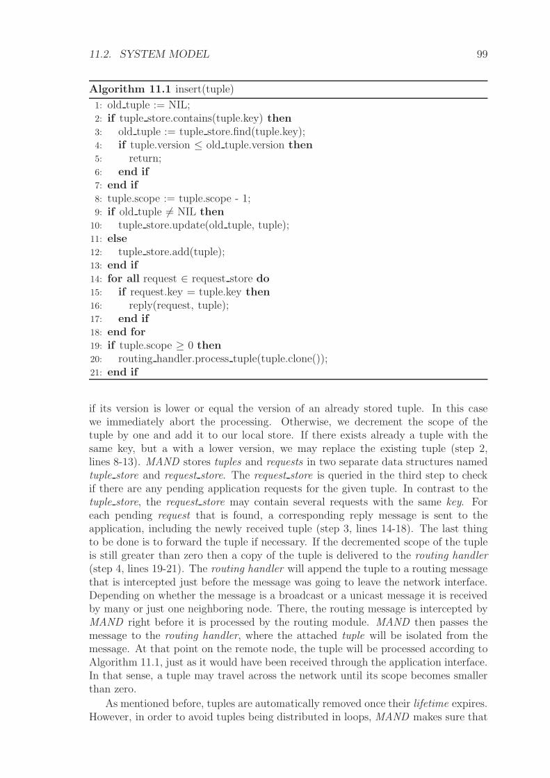
11.2. SYSTEM MODEL 99
Algorithm 11.1 insert(tuple)
1: old tuple := NIL;2: if tuple store.contains(tuple.key) then3: old tuple := tuple store.find(tuple.key);4: if tuple.version ≤ old tuple.version then5: return;6: end if7: end if8: tuple.scope := tuple.scope - 1;9: if old tuple 6= NIL then
10: tuple store.update(old tuple, tuple);11: else12: tuple store.add(tuple);13: end if14: for all request ∈ request store do15: if request.key = tuple.key then16: reply(request, tuple);17: end if18: end for19: if tuple.scope ≥ 0 then20: routing handler.process tuple(tuple.clone());21: end if
if its version is lower or equal the version of an already stored tuple. In this casewe immediately abort the processing. Otherwise, we decrement the scope of thetuple by one and add it to our local store. If there exists already a tuple with thesame key, but a with a lower version, we may replace the existing tuple (step 2,lines 8-13). MAND stores tuples and requests in two separate data structures namedtuple store and request store. The request store is queried in the third step to checkif there are any pending application requests for the given tuple. In contrast to thetuple store, the request store may contain several requests with the same key. Foreach pending request that is found, a corresponding reply message is sent to theapplication, including the newly received tuple (step 3, lines 14-18). The last thingto be done is to forward the tuple if necessary. If the decremented scope of the tupleis still greater than zero then a copy of the tuple is delivered to the routing handler(step 4, lines 19-21). The routing handler will append the tuple to a routing messagethat is intercepted just before the message was going to leave the network interface.Depending on whether the message is a broadcast or a unicast message it is receivedby many or just one neighboring node. There, the routing message is intercepted byMAND right before it is processed by the routing module. MAND then passes themessage to the routing handler, where the attached tuple will be isolated from themessage. At that point on the remote node, the tuple will be processed according toAlgorithm 11.1, just as it would have been received through the application interface.In that sense, a tuple may travel across the network until its scope becomes smallerthan zero.
As mentioned before, tuples are automatically removed once their lifetime expires.However, in order to avoid tuples being distributed in loops, MAND makes sure that

100 CHAPTER 11. MAND: MOBILE AD HOC NETWORK DIRECTORY
Algorithm 11.2 lookup(request) : tuple
1: request.scope := request.scope - 1;2: is fresh := true;3: if request store.contains(request.key) then4: old request := request store.find(request.key);5: if old request.version ≥ request.version then6: is fresh := false;7: else if old request.owner = request.owner then8: request store.add(request);9: end if
10: end if11: if tuple store.contains(request.key) then12: tuple := tuple store.find(request.key);13: if is local(request.key) then14: reply(request, tuple);15: else if is fresh then16: routing handler.process reply(request, tuple);17: end if18: else if is fresh ∧ request.scope ≥ 0 then19: routing handler.process request(request);20: end if
every tuple is stored for at least lmin seconds. Tuples with a lifetime of less than lminwill be cached for additional lmin − lifetime seconds. During that time, the tuple isconsidered to be in the invisible state, meaning that it cannot be looked up by anynode in the network. Invisible tuples prevent the distribution of tuples entering thesystem with the same key.
11.2.3 Looking up a tuple
When a request enters a node through the lookup(request) interface, it gets pro-cessed as follows (Algorithm 11.2). First, its scope value is decremented (line 1).Second, the system checks whether there is a already a matching request in the localrequest store. Remember, that two requests match only if they have a common key,version and owner. If no matching request was found, the new request is added tothe request store. Should there exist an old request with the same key and owner,but with an older version, then the old request will be replaced (lines 3-12). In bothcases we say the received request is fresh. In a third step, we check whether we canfind a tuple for the requested key in the local tuple store (lines 13-14). If a matchingtuple can be found, and the request was issued from a local application, then a replymessage will be sent to the application including the found tuple (lines 15-16). If,however, the request has been received from the network, and the request is fresh,then the found tuple together with the request is delivered to the routing handler(line 17-18). The routing handler makes sure the tuple will be sent back to the ownerof the request in an efficient way. More details on the internals of the routing handlerare presented in section 11.3. If, after all, no tuple matching the input request canbe found in the local tuple store, then the request is passed to the routing handler

11.3. ROUTING HANDLER 101
to be forwarded further (lines 17-19). Note that, as with the tuple, a request is onlyforwarded if it is fresh and its scope is greater or equal than zero. Generally, theforwarding of a request results in the same set of actions as the forwarding of a tuple.The routing handler attaches the request onto an existing routing message. On aneighboring node, the request is detached from the message by the routing handlerand it will again be processed as described in Algorithm 11.2.
11.3 Routing handler
So far we have seen how the routing handler is involved while storing or looking upa tuple. In general, the routing handler plug-in makes it possible for MAND to takeadvantage of the routing protocol’s mechanisms to forward and lookup tuples, whileat the same time not being dependent on the actual routing protocol used. Thedifficulty is to design a minimal interface between the routing handler and MANDwhich is powerful enough to support most types of routing protocols.
We have modelled the routing handler as a passive component that is invoked byMAND using the following five function calls:
• parse(routing message) is invoked whenever a new routing message is inter-cepted. The routing handler must parse the routing specific part of the messageand provide access to all extra data attached to a routing message.
• process tuple(tuple) is called by MAND whenever a tuple needs to be forwardedaccording to Algorithm 11.1. The routing handler may store the tuple tem-porarily until a routing message becomes available for piggybacking.
• process request(request) is called by MAND whenever a request needs to beforwarded according to Algorithm 11.2. Similar to the process tuple function,the routing handler is supposed to piggyback the request as soon as a routingmessage becomes available.
• process reply(request, tuple, routing message) is called whenever a request re-ceived from a remote node matches a tuple in the local store. MAND expectsthe routing handler to make sure the matching tuple is sent back to the ownerof the request (see Algorithm 11.2).
• piggyback(routing message) is called by MAND before a routing message isgoing to leave the NIC node. The routing handler may use the routing messageto piggyback tuples and requests it has received during previous process tupleor process request function calls.
A routing handler for a concrete routing protocol will have to provide implemen-tations for those five functions. Thereby, a routing handler should try to exploit therouting mechanism of the corresponding routing protocol. There is a vast amount ofdifferent approaches to perform routing in ad hoc networks. However, most existingrouting protocols either belong to the class of pro-active or to the class of reactiverouting protocols. Pro-active protocols maintain fresh lists of destinations and theirroutes by periodically distributing routing tables throughout the network. Reactiveprotocols find routes on demand by flooding the network with route request packets

102 CHAPTER 11. MAND: MOBILE AD HOC NETWORK DIRECTORY
Figure 11.2: Piggybacking MAND tuples onto an AODV routing message
whenever there is an application request. We have implemented two examples of arouting handler for both a pro-active, and a re-active routing protocol.
11.3.1 OLSR
OLSR is a pro-active routing protocol. The OLSR routing handler makes use ofthe fact that OLSR periodically advertises its routing table. More precisely, therouting handler temporarily stores tuples it has received through the process tupleinterface, and piggybacks them onto OLSR route advertisement messages wheneverthe piggyback function is invoked. The actual piggybacking is done by storing thetuple information inside an OSLR extension message as specified in [114]. OLSR ispurely pro-active and does not provide explicit route request functionality. Hence,the OLSR routing handler implements the process request interface by piggybackingrequests onto OLSR route advertisements, just as they would be regular tuples. Re-member that, whenever a remote request matches a tuple in a remote tuple store, theprocess reply function of the routing handler is called. The OLSR routing handlerimplements the process reply interface by sending a unicast UDP packet includingthe matching tuple to the owner of the request. The format of the message sent isthe same as the one of messages exchanged between a local application and MAND.
11.3.2 AODV
AODV is a re-active routing protocol. Thus, there are no periodic route advertisementmessages that could be used to piggyback tuples. Instead, the AODV routing handlerpiggybacks tuples onto route request and route reply messages that are issued byAODV on behalf of application requests. Additionally, the routing handler may alsopiggyback tuples onto AODV HELLO messages if available. The RFC [93] definesthose messages as optional, but in practice most implementations do use HELLOmessages to increase the robustness of the protocol. Piggybacking tuples is doneby storing the tuple information inside an AODV extension (see Figure 11.2), asspecified in [96]. The maximum size of an AODV extension is limited by 255 bytesdue to an 8 bit length field in the extension header. Therefore, the AODV routinghandler fragments tuples with a larger size into multiple data blocks of smaller sizeand spreads them across multiple AODV extensions.
One strength of AODV is its ability to discover routes on demand. AODV adoptsan expanding ring search technique where the network search region for a route re-quest is doubled in each phase until either the target node is found or the entire

11.4. INTERFACE SEMANTICS 103
network is reached. The AODV routing handler exploits this mechanism when beingasked to forward a request for a tuple. Upon receiving a process request call, the han-dler temporarily stores the submitted request and triggers an AODV route request.The newly triggered route request message is intercepted by MAND immediately andpassed to the handler’s piggyback function where the previously stored request is at-tached. Triggering a route request can be done without interacting with the routingprotocol directly, for instance by transmitting a UDP packet to an IP address thatdoes not exist in the ad hoc network. MAND manages a pool of configurable IPaddresses to be used for this purpose.
Any routing handler must implement the process reply interface to guaranteethat tuples matching remote requests are actually sent back to the originator of therequest. The AODV routing handler, when being invoked by a process reply functioncall, stores the matching tuple and triggers a route reply. The triggered AODV routereply message is intercepted immediately by MAND and passed to the handler’spiggyback function where the previously stored tuple is attached. Triggering a routereply, given the route request, is done simply by overwriting the route request’sdestination to be the local IP address. The altered route request message appears toAODV like a route request for the local node and makes AODV respond with a routereply message.
Overall, the AODV routing handler entirely maps a remote tuple lookup to theAODV route-request/route-reply procedure. By doing so, it is guaranteed that foreach successful remote MAND lookup request a route will be established to the nodehosting the requested tuple. This is of particular importance if the requested tuplecontains information about a service running on the host node. Obviously, the timespent to remotely look up a tuple is saved later when accessing the service since noroute establishment is needed anymore.
It is important to note that neither the AODV nor the OLSR routing handlerinteract with the routing protocol directly. The advantage is that the routing protocoldoes not have to be modified or re-compiled. This is a necessary requirement whenusing MAND in practice since users may not have control over the routing protocolimplementation.
11.4 Interface Semantics
In section 11.1 we discussed the various trade-offs involved in implementing a dis-tributed directory service. In MAND the behavior is controlled using the two fieldsscope and lifetime. These fields are available in both request and tuple and thus areexposed to the application level API (insert and lookup).
11.4.1 Controlled insertion of tuples
The advantages and disadvantages of a local versus a replicated insertion strategyhave been demonstrated in section 11.1. Using the scope parameter of a tuple, a userof MAND can configure any point of operation between local and fully replicated.
An application may use the lifetime parameter of a tuple together with the tupleupdate frequency adapt to the dynamics of the network. A tuple can be kept per-sistent in the network if it is periodically updated with a newer version before the

104 CHAPTER 11. MAND: MOBILE AD HOC NETWORK DIRECTORY
Figure 11.3: Example 3: Event/Subscription. Tuple request with scope > 0 andlifetime > 0. Tuple insert with scope = 0 and lifetime> 0
Figure 11.4: Example 2: Remote lookup. Tuple request with scope > 0 andlifetime > 0. Tuple insert with scope = 0 and lifetime> 0
lifetime expires. A short lifetime could be useful to avoid stale and outdated tuplesin a MANET that is exposed to network partitions. Network partitions may preventa node from receiving the latest update for a tuple. With the lifetime being shorttogether with an appropriate update frequency, it is guaranteed those tuples will beeither be up to date or removed quickly. On the other hand, a long tuple lifetime isused if the network topology does not change often or if tuple updates are rare. If thelifetime of a tuple is set to zero, a tuple will not be stored in the tuple store of thenode. It will, however, be forwarded if its scope is large enough. We call those tuplesevents, since they trigger reply messages for pending local requests (see Algorithm11.2). Figure 11.3 illustrates the distribution of an event. Node B in Figure 11.3has issued a request with a large lifetime to make sure it is notified whenever anevent is received for the specified key. Since the event is not stored in MAND onintermediate nodes, any subsequent event for the same key will be considered as freshand therefore will be forwarded (see Algorithm 11.1). This allows for events sharinga common key to be triggered by different nodes in the network.

11.4. INTERFACE SEMANTICS 105
Figure 11.5: Example 1: Polling. Tuple request with scope=0 and lifetime=0.Tuple insert with scope > 0 and lifetime> 0
11.4.2 Controlled lookup of tuples
When searching for a tuple using the MAND lookup interface, an application mayuse the scope parameter to limit the network search region in terms of hops. Inpractice, a lookup with a large scope is often combined with a rather small scopeduring tuple insertion. The scope value used during an insert or lookup operationmirrors the frequency in which those operations take place. One typical use case forrequests with a large scope are situations where searching is a rare but an importantoperation. In this case we shift some of the communication cost incurring duringtuple insertion to the lookup operation. When using an on-demand routing protocol,we have seen in section 11.3.2 that the lookup costs might be compensated laterbecause no additional route establishment will be necessary. Figure 11.4 illustrates aremote tuple lookup. There, the request is issued with a scope > 0 whereas the tupleis inserted with scope = 0. Note that the request has a lifetime (white bar in Figure11.4) specifying the time window during which matching tuples will be accepted.There are also good reasons to issue tuple requests with a small scope. A scope ofzero for instance can be used to make sure the search query is applied only to thelocal MAND instance.
An application may use the lifetime parameter of a tuple request to control thetime MAND waits until it receives tuples with the requested key. In some cases, ap-plications may not want to wait at all. Then the best they can do is to issue a requestwith zero lifetime and zero scope. If a matching tuple is found, a response includingthe matching tuple is sent back to the application. If no matching tuple is found, therequest expires immediately causing a negative acknowledgment (NACK) to be sentback to the application. In either case, the tuple request call is non-blocking, whichis a requirement in many applications. In Figure 11.5, the application periodicallyperforms a local lookup with scope and lifetime set to zero. In the example, the firsttwo requests are replied with a NACK until the third request successfully returns therequested tuple. The tuple has been distributed in the network due to an insert of atuple with scope > 0 on a remote node. Note that, while the tuple was distributed inthe network, every node who is forwarding the tuple will also store a copy of it in itslocal tuple store. Figure 11.5 also illustrates the lifetime of a tuple (grey bar). Thelifetime starts on every node at the moment the tuple is received. Hence, different
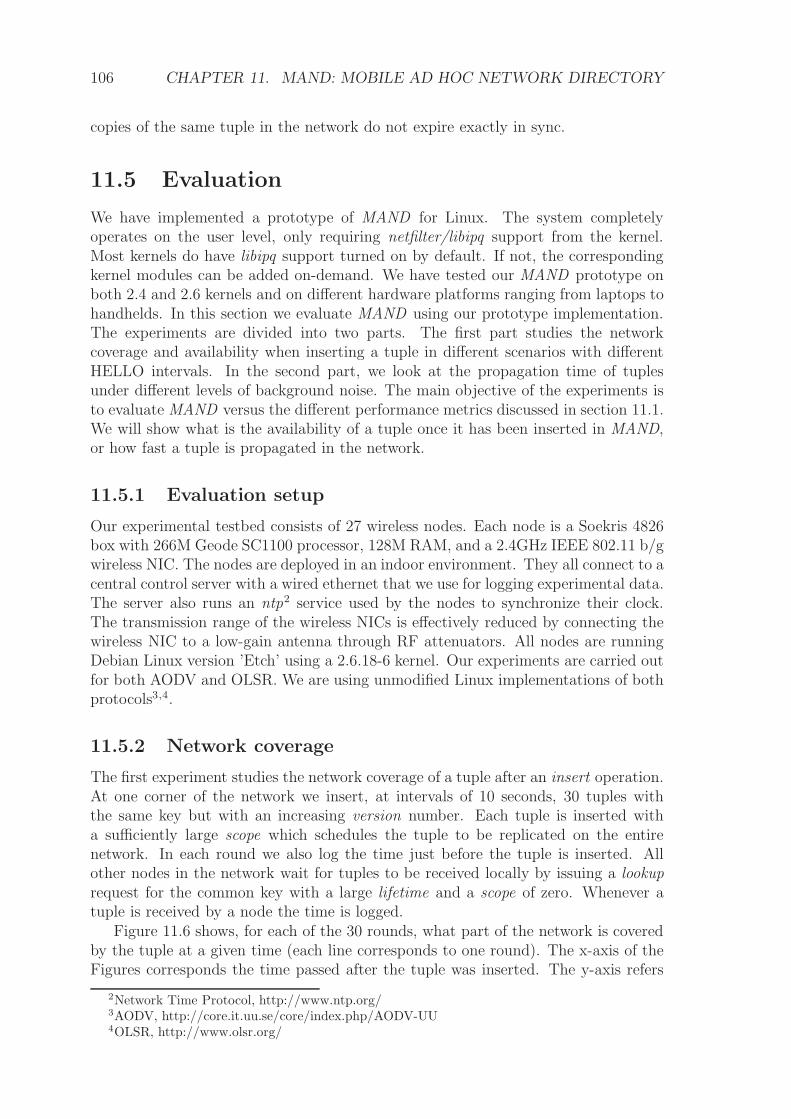
106 CHAPTER 11. MAND: MOBILE AD HOC NETWORK DIRECTORY
copies of the same tuple in the network do not expire exactly in sync.
11.5 Evaluation
We have implemented a prototype of MAND for Linux. The system completelyoperates on the user level, only requiring netfilter/libipq support from the kernel.Most kernels do have libipq support turned on by default. If not, the correspondingkernel modules can be added on-demand. We have tested our MAND prototype onboth 2.4 and 2.6 kernels and on different hardware platforms ranging from laptops tohandhelds. In this section we evaluate MAND using our prototype implementation.The experiments are divided into two parts. The first part studies the networkcoverage and availability when inserting a tuple in different scenarios with differentHELLO intervals. In the second part, we look at the propagation time of tuplesunder different levels of background noise. The main objective of the experiments isto evaluate MAND versus the different performance metrics discussed in section 11.1.We will show what is the availability of a tuple once it has been inserted in MAND,or how fast a tuple is propagated in the network.
11.5.1 Evaluation setup
Our experimental testbed consists of 27 wireless nodes. Each node is a Soekris 4826box with 266M Geode SC1100 processor, 128M RAM, and a 2.4GHz IEEE 802.11 b/gwireless NIC. The nodes are deployed in an indoor environment. They all connect to acentral control server with a wired ethernet that we use for logging experimental data.The server also runs an ntp2 service used by the nodes to synchronize their clock.The transmission range of the wireless NICs is effectively reduced by connecting thewireless NIC to a low-gain antenna through RF attenuators. All nodes are runningDebian Linux version ’Etch’ using a 2.6.18-6 kernel. Our experiments are carried outfor both AODV and OLSR. We are using unmodified Linux implementations of bothprotocols3,4.
11.5.2 Network coverage
The first experiment studies the network coverage of a tuple after an insert operation.At one corner of the network we insert, at intervals of 10 seconds, 30 tuples withthe same key but with an increasing version number. Each tuple is inserted witha sufficiently large scope which schedules the tuple to be replicated on the entirenetwork. In each round we also log the time just before the tuple is inserted. Allother nodes in the network wait for tuples to be received locally by issuing a lookuprequest for the common key with a large lifetime and a scope of zero. Whenever atuple is received by a node the time is logged.
Figure 11.6 shows, for each of the 30 rounds, what part of the network is coveredby the tuple at a given time (each line corresponds to one round). The x-axis of theFigures corresponds the time passed after the tuple was inserted. The y-axis refers
2Network Time Protocol, http://www.ntp.org/3AODV, http://core.it.uu.se/core/index.php/AODV-UU4OLSR, http://www.olsr.org/
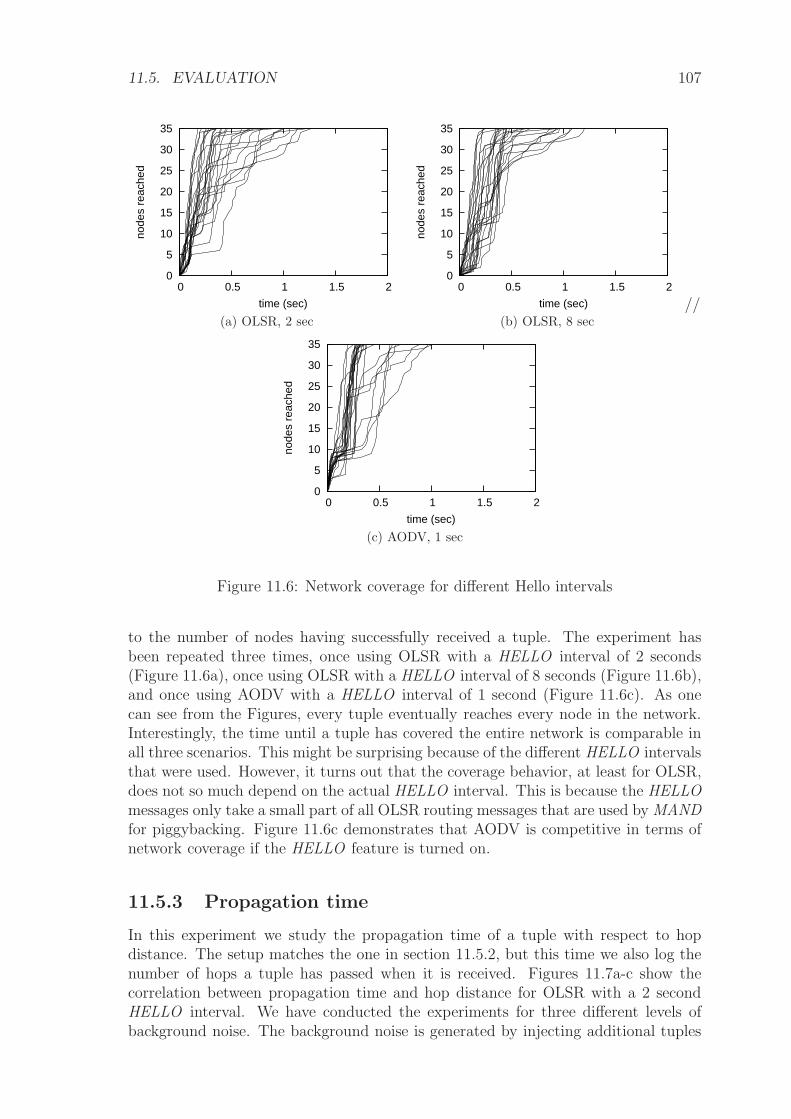
11.5. EVALUATION 107
0
5
10
15
20
25
30
35
0 0.5 1 1.5 2
node
s re
ache
d
time (sec)
(a) OLSR, 2 sec
0
5
10
15
20
25
30
35
0 0.5 1 1.5 2
node
s re
ache
d
time (sec)
(b) OLSR, 8 sec//
0
5
10
15
20
25
30
35
0 0.5 1 1.5 2
node
s re
ache
d
time (sec)
(c) AODV, 1 sec
Figure 11.6: Network coverage for different Hello intervals
to the number of nodes having successfully received a tuple. The experiment hasbeen repeated three times, once using OLSR with a HELLO interval of 2 seconds(Figure 11.6a), once using OLSR with a HELLO interval of 8 seconds (Figure 11.6b),and once using AODV with a HELLO interval of 1 second (Figure 11.6c). As onecan see from the Figures, every tuple eventually reaches every node in the network.Interestingly, the time until a tuple has covered the entire network is comparable inall three scenarios. This might be surprising because of the different HELLO intervalsthat were used. However, it turns out that the coverage behavior, at least for OLSR,does not so much depend on the actual HELLO interval. This is because the HELLOmessages only take a small part of all OLSR routing messages that are used by MANDfor piggybacking. Figure 11.6c demonstrates that AODV is competitive in terms ofnetwork coverage if the HELLO feature is turned on.
11.5.3 Propagation time
In this experiment we study the propagation time of a tuple with respect to hopdistance. The setup matches the one in section 11.5.2, but this time we also log thenumber of hops a tuple has passed when it is received. Figures 11.7a-c show thecorrelation between propagation time and hop distance for OLSR with a 2 secondHELLO interval. We have conducted the experiments for three different levels ofbackground noise. The background noise is generated by injecting additional tuples

108 CHAPTER 11. MAND: MOBILE AD HOC NETWORK DIRECTORY
0
0.5
1
1.5
2
2.5
3
3.5
4
0 1 2 3 4 5 6
time
[sec
]
distance [#hops]
(a) Background noise, 1 tuple per 8 seconds
0
0.5
1
1.5
2
2.5
3
3.5
4
0 1 2 3 4 5 6
time
[sec
]
distance [#hops]
(b) Background noise, 1 tuple per 4 seconds
0
0.5
1
1.5
2
2.5
3
3.5
4
0 1 2 3 4 5 6
time
[sec
]
distance [#hops]
(c) Background noise, 1 tuple per 2 seconds
Figure 11.7: Tuple propagation in OLSR with under tuple generation rates
on nodes performing the requests. Each point in Figures 11.7a-c corresponds to thereception of a tuple ’x’ hops away from the originator. The line shown in each Figurerefers to the average propagation time. For a HELLO message interval of p secondsthe maximum propagation time of a tuple traveling k hops is 2× k seconds.
A first observation from Figures 11.7a-c is that the measured propagation timestays significantly below the worst case value. This is because the tuples propagatewith a high redundancy. There is set of alternative paths between any node in thenetwork and the node at the corner where the insertion of the tuple takes place. Thepropagation time of a tuple along a given path is determined by the length of thepath and its schedule. Some paths may have a slow schedule. This is if a tuple,upon reception at a node, always just misses the next routing message. Some paths,however, might really have a fast schedule. This is if the reception of a tuple on anode is immediately followed by the transmission of a routing message. The tuplearriving first at a given receiver node is the one where the schedule and the pathlength did result in the fastest propagation time among all the different paths.
A second observation from Figures 11.7a-c is that the avarage propagation timeincreases with the background noise. This makes sense since tuples will have to stayin the queue for a longer time before they can be piggybacked. It can also be seenthat, the more tuple background noise we have, the higher the variations in the tuplearrival rate.

11.5. EVALUATION 109
0
0.2
0.4
0.6
0.8
1
1.2
1.4
0 1 2 3
look
up ti
me
[sec
]
scope
MAND/OLSRMAND/AODV
(a) Lookup time,OLSR
0
0.2
0.4
0.6
0.8
1
1.2
0 1 2 3 4 5 6
look
up ti
me
[sec
]
scope
AODVAODV/MANDOLSR/MAND
(b) Lookup time,AODV
Figure 11.8: MAND evaluation on the testbed: Lookup time
11.5.4 Lookup time vs. scope
In this experiment we study the time needed to remotely lookup a tuple. The setupmatches the one in section 11.5.2, except that we insert the tuple with four differentreplication levels (scope=0,1,2,3). A scope of zero means that the tuple is not repli-cated at all. A scope of 3 means that the tuple is replicated on all nodes that arereachable over 3 hops. Figure 11.8a shows the lookup time in each of those cases.As we can see, the lookup time decreases with the replication level of the tuple. Thisis because the higher the replication level, the more likely it is that a tuple can beretrieved from a closeby node.
11.5.5 Lookup time vs. Hop Distance
In this experiment we relate the tuple lookup time to the hop distance the tuple isaway from the requestor. For this purpose, a tuple with a scope of 0 and a lifetimeof 20 is inserted into MAND on one node of the network. Another node k hops awaymakes a MAND lookup call for that given tuple using a scope of 10 and a lifetimeof 20. The lookup time refers to the time from the moment the lookup call is madeuntil the requested tuple is returned.Figure 11.8b shows the measured lookup time when using AODV and OLSR as thead hoc routing protocol. As a reference, we also show the AODV route establishmenttime.
A first observation from Figure 11.8b is that the lookup time when running AODVis faster than the lookup time when running OLSR. This makes sense since the routinghandler for AODV integrates tuple requests directly with AODV’s RREQ/RREPmechanism, while for OLSR tuple requests are piggybacked just as regular tuples. Asecond observation from Figure 11.8b is that looking up a tuple using MAND andAODV only takes a few milliseconds longer than a simple AODV route request forthe same hop distance. Therefore, the price for piggybacking is minimal. The gap intime between three and four hops in Figure 11.8b is due to AODV’s expanded ringsearch technique [93], which we have discussed in section 11.3.2.

110 CHAPTER 11. MAND: MOBILE AD HOC NETWORK DIRECTORY
0
50
100
150
200
0 0.5 1 1.5 2 2.5 3 3.5 4
node
s re
ache
d
time (sec)
(a) Static nodes
0
50
100
150
200
0 0.5 1 1.5 2 2.5 3 3.5 4
node
s re
ache
d
time (sec)
(b) Moderate speed (up to 72 km/h)
0
50
100
150
200
0 0.5 1 1.5 2 2.5 3 3.5 4
node
s re
ache
d
time (sec)
(c) Fast speed (up to 180 km/h)
0
0.5
1
1.5
2
2.5
3
3.5
0 2 4 6 8 10 12 14 16 18 20
time
(sec
)
hops traversed
(d) Tuple propagation time vs. hop count, inproactive protocols (OLSR shown)
Figure 11.9: Tuple insertion over the OLSR protocol. Demonstrates the dynamics oftuple propagation in proactive protocols, by means of HELLO messages, for staticand mobile scenarios.
11.6 Simulation
In addition to deploying MAND on a real network, we also implemented it andsimulated it on NS2 [72]. Our basic configuration is a set of 50 nodes spread uniformlyat random across a 1500m×300m plane. In order to test our system in a larger scale,we also consider a configuration of 200 nodes spread across a plane of dimensions3000m × 600m, to keep the node density constant. We used the default AODVimplementation included in the NS simulator, and the Universidad de Murcia UM-OLSR [115] implementation for NS.
11.6.1 Inserting Tuples
Propagation Speed
We carried out a number of experiments to explore the dynamics of tuple propagationin proactive protocols. The first observation is that, unless tuples are discarded due toqueue overflow under congestion (see Section 11.6.1 below), they reach all nodes of thenetwork. In our experiments we never observed a tuple propagation being hindered bythe occasional packet collisions that occurred. This is due to the inherent redundancy

11.6. SIMULATION 111
in tuple propagation in proactive protocols, comprising numerous intermingled paths.
To observe the tuple propagation speed in proactive protocols, we ran MANDover a simulated network of 200 nodes running OLSR, introduced 50 tuples originat-ing at randomly selected nodes, and kept track of the times at which they reachedother nodes. To keep our measurements unbiased, we let tuples propagate at non-overlapping periods, and induced no traffic to the network. That is, only hello mes-sages were being exchanged by the routing protocol.
Figure 11.9 plots the number of nodes that have received a tuple as a function ofthe time elapsed since the first transmission of the tuple, for a static network and fortwo instances of mobile networks. All three scenarios demonstrate that all tuples arespread fast and reach all nodes.
It should be emphasized that node mobility does not affect the operation ofMAND. Quite on the contrary, it has a positive effect on it, accelerating the prop-agation of tuples. Figures 11.9(b) and (c) (nodes moving in random directions andat random speeds up to 72 km/h and 180 km/h, respectively) reveal lower propaga-tion times compared to the static network of Figure 11.9(a). This is a particularlyinteresting result, and the behavior of our system under mobility is of particular im-portance to our work. Figure 11.9(c) shows the correlation of hops traversed and therespective time for a static network running OLSR. As expected, this is on average alinear relationship.
Finally, it should be noted that we carried out the same experiments also overAODV, having configured it to send HELLO messages. Setting equal periods ofHELLO messages in the two protocols leads to indistinguishable results.
Tuple Forwarding History
In MAND tuples are forwarded whenever their scope is greater or equal than zeroand no existing tuple with the key is already available in the local store. In section11.2.2 we discussed that every tuple is stored for at least lmin seconds to avoid tuplesbeing propagated in a “ping-pong” fashion if their actual lifetime is small. We calllmin the the tuple forwarding history, which is the time we cache tuples that wererecently forwarded. A long history would serve our goal of redundance avoidance,but would consume more resources, both in terms of node memory as well as nodeprocessing. A very short history could prove inadequate in certain networks.
In this section we perform a series of experiments to determine the optimal historylength. Figure 11.10 shows the average number of times a tuple is forwarded by eachnode, as a function of the history length (in seconds). For very short history lengths,nodes “forget” tuples they have recently forwarded, and are willing to forward themagain upon subsequent reception. In fact, recycling of tuples would go on for ever,unless tuple propagation was limited by the scope field.
In Figure 11.10 we consider a network of 50 nodes, and tuples are inserted witha scope of ten. We can see that for a history length of two seconds or longer, tuplesare forwarded exactly once by each node, which is the desired behavior. Clearly, thiscrucial history length depends on the network topology and the cycles that can beformed. A good design should ensure that an adequate history length is allocatedper node, to avoid unnecessary tuple forwarding overhead and congestion.
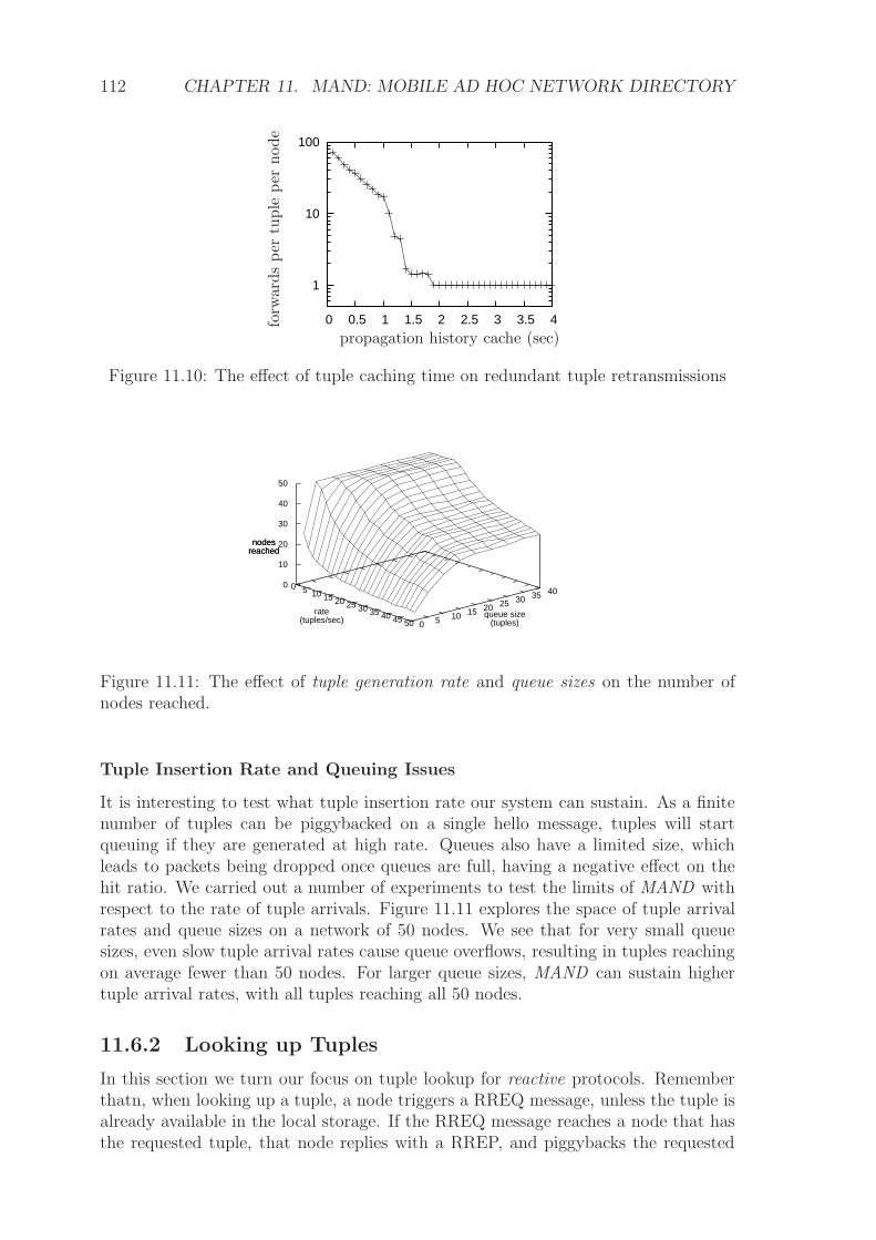
112 CHAPTER 11. MAND: MOBILE AD HOC NETWORK DIRECTORY
1
10
100
0 0.5 1 1.5 2 2.5 3 3.5 4
propagation history cache (sec)
forw
ards
per
tuple
per
node
Figure 11.10: The effect of tuple caching time on redundant tuple retransmissions
queue size(tuples)
rate(tuples/sec)
0
10
20
30
40
50
nodesreached
0 5 10 15 20 25 30 35 40 0 5 10 15 20 25 30 35 40 45 50
nodesreached
Figure 11.11: The effect of tuple generation rate and queue sizes on the number ofnodes reached.
Tuple Insertion Rate and Queuing Issues
It is interesting to test what tuple insertion rate our system can sustain. As a finitenumber of tuples can be piggybacked on a single hello message, tuples will startqueuing if they are generated at high rate. Queues also have a limited size, whichleads to packets being dropped once queues are full, having a negative effect on thehit ratio. We carried out a number of experiments to test the limits of MAND withrespect to the rate of tuple arrivals. Figure 11.11 explores the space of tuple arrivalrates and queue sizes on a network of 50 nodes. We see that for very small queuesizes, even slow tuple arrival rates cause queue overflows, resulting in tuples reachingon average fewer than 50 nodes. For larger queue sizes, MAND can sustain highertuple arrival rates, with all tuples reaching all 50 nodes.
11.6.2 Looking up Tuples
In this section we turn our focus on tuple lookup for reactive protocols. Rememberthatn, when looking up a tuple, a node triggers a RREQ message, unless the tuple isalready available in the local storage. If the RREQ message reaches a node that hasthe requested tuple, that node replies with a RREP, and piggybacks the requested

11.7. RELATED WORK 113
0
0.2
0.4
0.6
0.8
1
0 0.05 0.1 0.15 0.2 0.25 0.3 0.35 0.4pe
rcen
tage
of t
uple
slookup time (sec)
From top to bottom:scope 10, 8, 6, 4, 3, 2, 1, 0
Figure 11.12: CDF of tuple lookup times for AODV. Each line corresponds to tuplesspread with a different scope prior to their lookup.
tuple on it.
Clearly, the success rate and the lookup times depend on the extent at which thetuple in question is spread. In the extreme case that the tuple lays exclusively onits originating node, that specific node has to be reached by the requester’s RREQ,and the single RREP sent back has to reach the requester. This may induce higherdelays and more sensitivity to packet loss compared to the case of an abundantlyreplicated tuple, that would result in multiple RREP messages being send back tothe requester. The other extreme, of course, is a tuple spread to the whole network,in which case the requester has a copy of the tuple in its local storage.
Figure 11.12 shows the CDF of the lookup times in a network of 200 nodes ina 3000m by 600m plain, for tuples initially spread with scopes from 0 to 10. Notethat for non-replicated tuples (scope 0), lookup times are longer, and not all requestsare successful. As the replication level increases, we observe lower lookup times, andhigher success rates of lookups.
11.7 Related Work
In the past, there have been various different approaches to key based search inMANETs. Lindemann and Waldhorst showed how to apply epidemic dissemination toimplement a distributed directory and introduced an analytical performance modelingapproach [116, 117]. They presented a general-purpose distributed lookup service formobile applications, denoted Passive Distributed Indexing (PDI). PDI stores indexentries in form of (key, value) pairs in index caches maintained by each node. Indexcaches are filled by epidemic dissemination of popular index entries. Their approach,however, assumes that nodes are moving and exchanging cache entries whenever theyare physically close.
Another approach is to provide efficient lookup facilities rather than replicatingentries. Cell Hash Routing (CHR) [76] is a specialized ad-hoc DHT. CHR uses posi-tion information to construct a DHT of clusters instead of organizing individual nodesin the overlay. The limitations of this approach is that maintaining the cluster can bevery expensive under node mobility. Moreover, the approach is not generic enoughsince it requires position information of the nodes. Cramer and Fuhrmann [118] pro-
114 CHAPTER 11. MAND: MOBILE AD HOC NETWORK DIRECTORY
pose the Chord based Proximity Neighbor Selection Strategy (PNS CHORD). Here,the nodes are connected to their logical successors on the ring and through logicalshortcuts to further nodes as usual in Chord [119]. However, because the constructionof routing tables is absed on physical proximity, it may happen that the logical pathpursued by a request traverses the same node multiple times. This problem has beentackled in [79] where the authors propose an adaptive learning process to preventsuch loops. However, as all other DHT based approaches, also [79] is very inefficientwhen it comes the number actual messages that are transmitted per lookup request.This is because, transmitting a packet along an overlay may cause route requests onevery hop. Ekta [75] and MADPastry [77] integrate key lookup facilities with theAODV routing protocol. And pucha et at. [120] implements Pastry [121] on top ofDynamic Source Routing (DSR) [122]. Rowstron et al. propose VRR [123], a routingprotocol including logical DHT-like addressing. The problem all these approacheshave is that they rely on a particular routing protocol which is not useful in practice.
The problem of key based search has similarities with service discovery and nameresolution in MANETs. One approach to the latter is to let service information bemaintained on a per-cluster basis [124, 125]. However, electing and maintaining spe-cialized nodes is difficult and expensive due to the dynamic nature of MANETs. Infact, it has been shown that in terms of transmitted messages, a fully distributedservice discovery outperforms the per-cluster approach, especially in mobile scenar-ios [125].
Another related problem to key based search can be found in geographical rout-ing. Geographical routing algorithms assume the availability of geographical locationinformation of nodes (e.g., via GPS or other techniques). Using this informationnodes make packet forwarding decisions based on the packet destination location andneighboring nodes locations. To discover the location information, geographical rout-ing makes use of so called location services. In principle, the location service mapsa unique ID of a node, to the current location of the node. One approach to pro-vide location services is to divide the network area into a flat grid of squares, andthen store the location information of a node on all other nodes residing inside arandomly chosen square, dependent on the ID of the node and the coordinates of thesquare[126, 127, 128]. The disadvantage of this approach is that the routing costs toquery the location of a node grow proportional to the network size, even if the two par-ticapting nodes are geographically close to each other. To improve the performance oflocation services hierarchical directory structures were suggested [129, 130, 131, 132].In those approaches, position information is stored on a hierarchy of regions (squares)and lookup requests are routed along a list of pointers mapping the logical hierachyto the physical network topology. The disadvantage of such an approach is that –similar to cluster based service discovery [124, 125] – maintaining the hierarchicalstructure becomes an expensive task under node mobility.
11.8 Summary
In this chapter we have presented MAND, a novel infrastructure for implementingnetworking services in mobile ad hoc networks. MAND builds upon the observa-tion that many networking services can be seen as mapping functions. Accordingly,MAND implements an efficient mechanism for storing, distributing, and searching

11.8. SUMMARY 115
tuples (key/value) pairs in MANETs. MAND differs from existing work in that itcombines three properties in a unique way: a) parameterized modes of operation toaddress trade-offs such as update performance vs consistency or lookup performance;b) efficient integration with the underlying routing to minimize overhead and opti-mize the service access time for network services using MAND ; c) independence ofthe type of the underlying routing protocol. Using these ideas, we have implementedMAND over several routing protocols and deployed it on a test-bed consisting of 30wireless nodes. By extensive experimentation we have shown that MAND performsvery well in different settings and different modes of operation. To show the potentialand prove the feasibility of MAND, we have implemented several networking servicesthat make MANETs a seamless extension of infrastructure based networks.

116 CHAPTER 11. MAND: MOBILE AD HOC NETWORK DIRECTORY
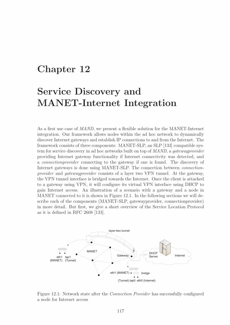
Chapter 12
Service Discovery andMANET-Internet Integration
As a first use case of MAND, we present a flexible solution for the MANET-Internetintegration. Our framework allows nodes within the ad hoc network to dynamicallydiscover Internet gateways and establish IP connections to and from the Internet. Theframework consists of three components: MANET-SLP, an SLP [133] compatible sys-tem for service discovery in ad hoc networks built on top of MAND, a gatewayproviderproviding Internet gateway functionality if Internet connectivity was detected, anda connectionprovider connecting to the gateway if one is found. The discovery ofInternet gateways is done using MANET-SLP. The connection between connection-provider and gatewayprovider consists of a layer two VPN tunnel. At the gateway,the VPN tunnel interface is bridged towards the Internet. Once the client is attachedto a gateway using VPN, it will configure its virtual VPN interface using DHCP togain Internet access. An illustration of a scenario with a gateway and a node inMANET connected to it is shown in Figure 12.1. In the following sections we will de-scribe each of the components (MANET-SLP, gatewayprovider, connectionprovider)in more detail. But first, we give a short overview of the Service Location Protocolas it is defined in RFC 2608 [133].
Internet
MANETDHCPServer
layer-two tunnel
Gateway
eth1 (MANET) bridge
(Tunnel) tap0 eth0 (Internet)
eth1(MANET)
tap1(Tunnel)
Figure 12.1: Network state after the Connection Provider has successfully configureda node for Internet access
117
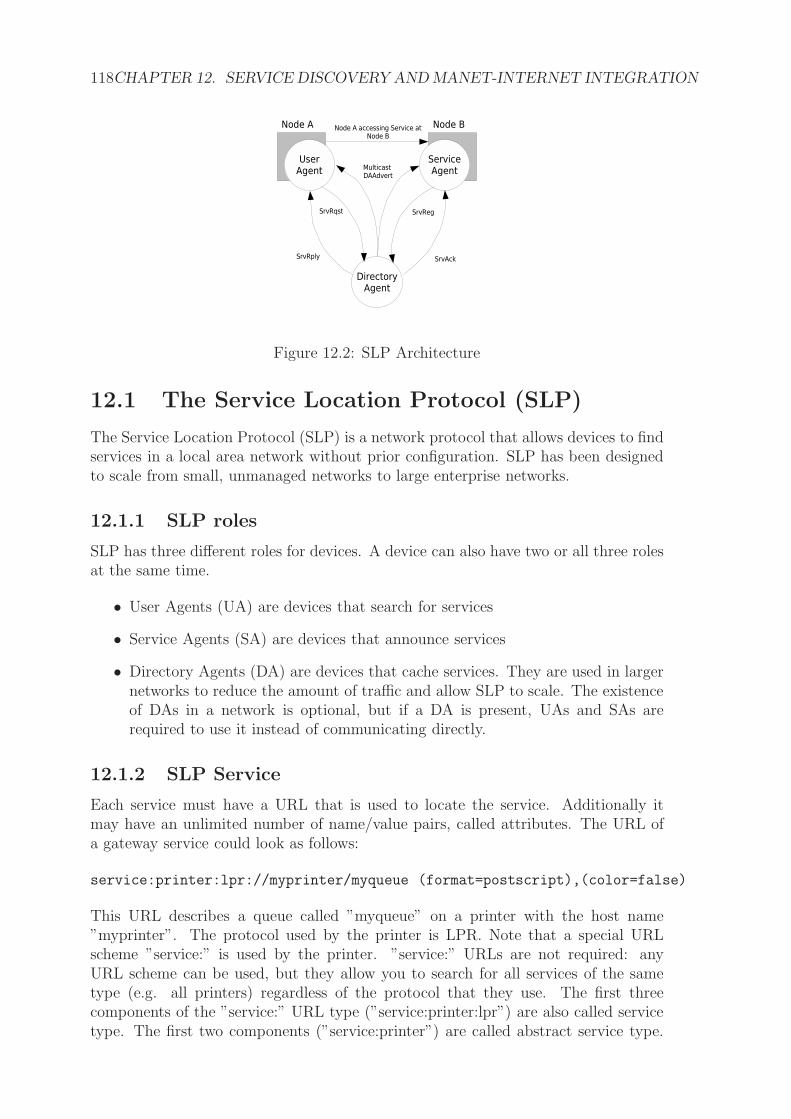
118CHAPTER 12. SERVICE DISCOVERY AND MANET-INTERNET INTEGRATION
Figure 12.2: SLP Architecture
12.1 The Service Location Protocol (SLP)
The Service Location Protocol (SLP) is a network protocol that allows devices to findservices in a local area network without prior configuration. SLP has been designedto scale from small, unmanaged networks to large enterprise networks.
12.1.1 SLP roles
SLP has three different roles for devices. A device can also have two or all three rolesat the same time.
• User Agents (UA) are devices that search for services
• Service Agents (SA) are devices that announce services
• Directory Agents (DA) are devices that cache services. They are used in largernetworks to reduce the amount of traffic and allow SLP to scale. The existenceof DAs in a network is optional, but if a DA is present, UAs and SAs arerequired to use it instead of communicating directly.
12.1.2 SLP Service
Each service must have a URL that is used to locate the service. Additionally itmay have an unlimited number of name/value pairs, called attributes. The URL ofa gateway service could look as follows:
service:printer:lpr://myprinter/myqueue (format=postscript),(color=false)
This URL describes a queue called ”myqueue” on a printer with the host name”myprinter”. The protocol used by the printer is LPR. Note that a special URLscheme ”service:” is used by the printer. ”service:” URLs are not required: anyURL scheme can be used, but they allow you to search for all services of the sametype (e.g. all printers) regardless of the protocol that they use. The first threecomponents of the ”service:” URL type (”service:printer:lpr”) are also called servicetype. The first two components (”service:printer”) are called abstract service type.
12.2. MANET-SLP 119
The attributes of the printer are specified in the last part of the service description(”(format=postscript),(color=false)”). The example uses the standard syntax forattributes in SLP.
12.1.3 SLP Queries
SLP allows several query types to locate services and obtain information about them.It can search for all services with the same service type or abstract service type. Thequery can be combined with a query for attributes, using LDAP’s query language.
12.1.4 Protocol
SLP is a packet-oriented protocol. Most packets are transmitted using UDP, butTCP can also be used for the transmission of longer packets. Because of the potentialunreliability of UDP, SLP repeats all multicasts several times in increasing intervalsuntil an answer has been received. All devices are required to listen on port 427 forUDP packets, SAs and DAs should also listen for TCP on the same port. Multicastingis used extensively by SLP, especially by devices that join a network and need to findother devices. Figure 12.2 illustrates the SLP Architecture in a situation with nodes,A and B, where node A is requesting a service from node B.
12.2 MANET-SLP
MANET-SLP is a fully distributed service discovery platform for MANETs. It pro-vides a regular SLP interface for service registration and lookup. Services can be reg-istered using the SLP REGISTER interface and looked up using the SLP LOOKUPinterface. Logically, MANET-SLP resides on top of MAND. However, rather thanstoring service information into the MAND system, MANET-SLP uses MAND todistribute SLP events across the network, similar as shown in Figure 11.3. SupposeMANET-SLP receives a request to register the printer service we have described pre-viously. MANET-SLP will cache the service information locally and additionally itwill insert the following tuple into the MAND system:
tuple
key=slp,
value=service:printer:lpr://myprinter/myqueue
(format=postscript)(color=false)
service-lifetime=<service-lifetime>,
lifetime=0,
scope=<scope>
All tuples exchanged between MANET-SLP and MAND belong to the slp namespaceand thus have a common key. Every tuple is issued with a lifetime of zero. Asa consequence, the tuple is not stored in MAND, but is triggering events to allcurrent subscriptions for key=slp. Every MANET-SLP instance running on a nodemaintains such a subscription with the underlying MAND system. The subscriptionhas previously been issued and is periodically renewed using a MAND lookup call
120CHAPTER 12. SERVICE DISCOVERY AND MANET-INTERNET INTEGRATION
for the key slp. The tuple request passed to the MAND lookup interface may look asfollows:
request
key=slp,
lifetime=100,
scope=0
The zero scope of the tuple request makes sure the request is not propagated into thenetwork. The lifetime of 100 makes sure that the request stays in the MAND systemfor 100 seconds. During this period, MAND delivers all tuples with key “slp” toMANET-SLP. Before the lifetime of the request expires, MANET-SLP will re-insertthe request to update the subscription.
For every event MANET-SLP receives, MANET-SLP will store the service infor-mation given by tuple’s value in its local cache. How long a service information iscached locally is determined by the service lifetime which is an optional parameter ofthe SLP interface. If it is specified upon calling SLP REGISTER, the service-lifetimewill be encoded into the tuple value during the MAND insert call, which makes theservice-lifetime available to remotely cached services. SLP services registered withMANET-SLP may have a special attribute scope. The value of the scope attributeis directly mapped to the scope of the corresponding MAND tuple, thus determiningthe visibility of the service in the ad hoc network. There are default values for bothservice-lifetime and scope that can be defined upon system startup.
SLP Lookukp queries received by MANET-SLP will be answered just by con-sulting the local cache. There might be multiple services matching a given request.In MANET-SLP, all the service related information is exchanged pro-actively usingMAND, therefore no additional traffic is imposed to the network.
12.3 MANET-Internet integration
The MANET-SLP service can be leveraged to build a complete MANET-Internetintegration.
12.3.1 Gateway Provider
A Gateway Provider is a process that can set up a node to become a gateway in casethe node has Internet connection, and removes the gateway functionality in case theInternet connection is lost. Gateway Provider processes are started on nodes willingto act as gateways. A gateway is a node that is directly connected to the Internet andconfigured to provide Internet access to all the nodes within the MANET. Typically,these are nodes with multiple interfaces, since one interface is configured for com-munication with the MANET, and another interface is dynamically attached to theInternet. How a Gateway Provider works is shown in Figure 12.3. Once started, theGateway Provider process keeps waiting for an Internet connection to become avail-able (Figure 12.3, step 1). Detecting whether a node has Internet connection or not isdone using a special InternetDetectionAPI. The idea is to exploit system support toefficiently detect a possible Internet connection. Our current implementation makes

12.3. MANET-INTERNET INTEGRATION 121
(5) Publish Gateway Service:service:gw://192.168.220.x
EthernetBridge
GatewayProvider
MANET SLP
(3) Create tap0
(2) CreateBridge Deviceand add eth0
(4) Add tap0
(1) Wait forInternet Connection
on device eth0
layer-twotunneling
Figure 12.3: Gateway Provider
use of the operating system routing table. If an Internet connection has successfullybeen detected, say on interface eth0, the Gateway Provider process then creates abridge device on that node and immediately adds interface eth0 to the bridge (step2). In a following step, a layer-two tunnelling device tap0 is created (step 3) and alsoadded to the bridge (step 4). The device tap0 allows any node within the MANETto set up a layer-two tunnel connection to the gateway node. Since the tunnel devicetap0 is part of the bridge, traffic received on tap0 is directly forwarded to the Inter-net via interface eth0. To provide MANET nodes with such gateway functionality,a Gateway Provider must however first register itself as a gateway service using theunderlying MANET SLP service (step 5). The SLP service description may look asfollows:
service:gateway:manet://10.4.0.17
Once a gateway service is registered, any node within the MANET may look up thegateway’s location and connect to it. If the Internet connection is lost the service willbe de-registered or will timeout, and both the tunnel endpoint tap0 and the bridgewill be removed.
12.3.2 Connectionprovider
A Connection Provider is a process that sets up an Internet connection if a gatewaycan be found. Connection Provider processes are started on nodes who want anInternet connection. How a Connection Provider works is shown in Figure 12.4. Oncestarted, the Connection Provider process periodically searches for a gateway serviceby performing an SLP lookup request (Figure 12.4, step 1). If a gateway servicecan be found1, a layer-two tunnel connection to the gateway is established (step2). To finally configure the node for Internet access, a DHCP request is triggeredon that newly established tap1 interface (step 3). Since the tap0 interface at thegateway node is bridged towards the Internet, the DHCP request will eventuallybe answered by the DHCP server that is reachable from the gateway node. The
1Currently, if multiple gateway services are found, the list of all gateways is passed to the tun-nelling component
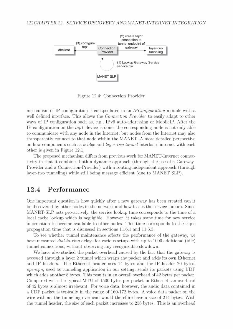
122CHAPTER 12. SERVICE DISCOVERY AND MANET-INTERNET INTEGRATION
(1) Lookup Gateway Service:service:gw
layer-twotunneling
ConnectionProvider
MANET SLP
(2) create tap1:connection to
tunnel endpoint ofgateway
(3) configuretap1
dhclient
Figure 12.4: Connection Provider
mechanism of IP configuration is encapsulated in an IPConfiguration module with awell defined interface. This allows the Connection Provider to easily adapt to otherways of IP configuration such as, e.g., IPv6 auto-addressing or MobileIP. After theIP configuration on the tap1 device is done, the corresponding node is not only ableto communicate with any node in the Internet, but nodes from the Internet may alsotransparently connect to that node within the MANET. A more detailed perspectiveon how components such as bridge and layer-two tunnel interfaces interact with eachother is given in Figure 12.1.
The proposed mechanism differs from previous work for MANET-Internet connec-tivity in that it combines both a dynamic approach (through the use of a Gateway-Provider and a Connection-Provider) with a routing independent approach (throughlayer-two tunneling) while still being message efficient (due to MANET SLP).
12.4 Performance
One important question is how quickly after a new gateway has been created can itbe discovered by other nodes in the network and how fast is the service lookup. SinceMANET-SLP acts pro-actively, the service lookup time corresponds to the time of alocal cache lookup which is negligible. However, it takes some time for new serviceinformation to become available to other nodes. This time corresponds to the tuplepropagation time that is discussed in sections 11.6.1 and 11.5.3.
To see whether tunnel maintenance affects the performance of the gateway, wehave measured dial-to-ring delays for various setups with up to 1000 additional (idle)tunnel connections, without observing any recognizable slowdown.
We have also studied the packet overhead caused by the fact that the gateway isaccessed through a layer 2 tunnel which wraps the packet and adds its own Ethernetand IP headers. The Ethernet header uses 14 bytes and the IP header 20 bytes.openvpn, used as tunneling application in our setting, sends its packets using UDPwhich adds another 8 bytes. This results in an overall overhead of 42 bytes per packet.Compared with the typical MTU of 1500 bytes per packet in Ethernet, an overheadof 42 bytes is almost irrelevant. For voice data, however, the audio data contained ina UDP packet is typically in the range of 160-172 bytes. A voice data packet on thewire without the tunneling overhead would therefore have a size of 214 bytes. Withthe tunnel header, the size of each packet increases to 256 bytes. This is an overhead

12.5. RELATED WORK 123
of 20%. If only a few nodes in the network communicate through the gateway usingtunneling this will not have a big effect. If the network is big and most of the userscommunicate through the gateway to the Internet, an overhead of 20% may decreasethe available capacity.
12.5 Related Work
12.5.1 Service Discovery
Some conventially adopted protocols, including Sun’s Jini [134], the service directoryservice UDDI [135], and IBM’s Salutation [136] rely on a central directory to regis-ter and discover services. Centralized architectures are inappropriate for MANETsbecause of the dynamic nature of such networks. Moreover, centralized directorieseasily suffer from routing bottlenecks.
Some distributed approaches, including Universal Plug and Play (UPnP) [137],Service Location Protocol (SLP) [133] of the IETF, and Bluetooth’s Service Discovery(SDP) [138], have been developed to reduce the overload of the centralized directory.However, those protocols are based on a network-wide multicast tree used for periodicservice advertisements. Multicast, however, is known to perform poorly in MANETs.
There are approaches specifically targeted at ad hoc networks. The distributedservice discovery protocol (DSDP) [139] has been developed to register the informa-tion of available services to a virtual backbone, and is based on clustering. A similarapproach has been proposed by [124]. However, electing and maintaining specializedbackbone nodes is difficult and expensive due to the mobility of MANETs. In fact, ithas been shown [125] that in terms of transmitted messages, a fully distributed ser-vice discovery outperforms the per-cluster approach, especially in mobile scenarios.To cope with mobile scenarios it has been suggested to integrate service discoverywith routing in MANETs. In [140], the authors propose to add extensions to theOn-Demand Multicast Routing Protocol (ODMRP) [141] to advertise service infor-mation. A similar approach was presented in [142, 143] based on the Optimized LinkState Routing Protocol and in [144] for the Ad Hoc On Demand Routing Protocol(AODV). It is true that by leveraging functionality of MANET routing protocols,service discovery can be improved, especially in terms of mobility support. However,we believe that a tight integration is impractical since it enforces service discoveryclients to use a specific routing protocol. This is a loss of freedom because there areplenty of different approaches for routing in MANETs, each of which has its ownadvantages and disadvantages in certain situations.
12.5.2 MANET-Internet integration
Dynamic gateway discovery has been combined with MANET routing [145]. Whilethis might be efficient, the solution is tailored to a specific routing protocol and notgeneralizable. Once a gateway is discovered, the challenge is to find ways to routeSIP and voice traffic through the gateway. In [146, 147, 148], specific functionalityof the given MANET routing protocol is exploited to forward data to the Internet.However, these solutions lack generality since they are routing specific. A routingindependent approach, where IP tunnelling is used between the end nodes and the
124CHAPTER 12. SERVICE DISCOVERY AND MANET-INTERNET INTEGRATION
gateway, can be found in [149], but their work requires gateway nodes to be locatedaccording to a fixed hierarchy. A more flexible design without topology assumptionsis described in [150, 151]. IPv6 auto-addressing for IP endpoint configuration hasbeen proposed in [145, 152], which is also not generic considering that IPv6 is notyet widely deployed. In order to provide a fixed IP endpoint to the outer world incase the gateway changes, Mobile IP has been suggested [150, 151, 146, 147, 148].Alternatively NAT is used for addressing. In the case of VoIP, a NAT approach wouldrequire some additional mechanisms like STUN [153] to allow peers located in theInternet to establish calls to nodes located within the MANET.
12.6 Summary
In this chapter we have presented MANET-SLP, a distributed and SLP compatiblesystem for service discovery in MANETs. Based on MANET-SLP we have describeda framework for MANET-Internet integration. The framework allows nodes in theMANET to communicate to and from the Internet as soon as one node in the adhoc network has Internet connectivity. In the next two chapters, we will make use ofthe MANET-Internet framework to allow DNS resolution and SIP routing to happenseamlessly accross the boundaries of MANET and Internet.
Chapter 13
DOPS: Domain Name andPresence Service
Another example of a standard networking service, besides SLP, is DNS. In this chap-ter, we describe a Domain Name and Presence Service (DOPS ) service, tailored toad hoc networks. DOPS provides a standard DNS interface but its implementation isin the form of a fully decentralized middleware platform. DOPS uses MAND as a di-rectory service and the MANET-Internet integration framework presented in the lastchapter to integrate seamlessly with the Internet. Moreover, DOPS naturally inter-links the ability to resolve a certain hostname with the presence of the correspondingnode in the network.
13.1 Standard DNS
Conceptually, DNS defines a tree where a node in the tree is identified by a particulardomain name. Each node is associated with a set of resource information, so calledresource records (RRs) [154]. Most importantly, resource records hold data like theIP address of a node. There are many different types of resource records, for instanceone to store an IPv4 address or one to store an IPv6 address. A DNS query namesthe domain name of interest and describes the type of resource information that isdesired. Nameservers hold information about some part of the domain tree’s structureand its associated resource records. The essential task of a name server is to answerqueries about the resource records the nameserver is associated with.
13.2 DOPS in the MANET
DOPS is a distributed domain name system running as a user space process oneach node in the ad hoc network1. Each DOPS instance stores the resource recordsassociated with the host node’s own domain name in MAND, thereby providing fullDNS access to all nodes in the network. To make use of DOPS a user has to justconfigure localhost to be the primary DNS contact address.
1DOPS may only run on a subset of nodes in a MANET; those that are interested to participatein a MANET-wide DNS system
125
126 CHAPTER 13. DOPS: DOMAIN NAME AND PRESENCE SERVICE
13.2.1 Mapping Resource Records to MAND Tuples
DNS resource records contain four important fields: The name specifies the domainname the RR is associated with. The type specifies the type of the RR (e.g., hostaddress type or a well known service description type). The class field identifies aprotocol family (e.g., IN for Internet System or CH for Chaos System). The ttl de-scribes how long a RR can be cached before it should be discarded. Finally, rddata isthe type dependent data which describes the resource (e.g., the actual host address).DOPS maps the structure of a RR to a MAND tuple as follows.
tuple
key=dns:<name>:<type>:<class>,
value=<rddata>,
lifetime=<ttl>,
scope=64
The name, the type and the class of the RR is used as a key of the tuple, the RRsrddata field (an IP address) forms the value. We use the RRs ttl to specify the lifetimeof the tuple. This makes sure that there are no stale RRs for nodes which are notpresent anymore in the network. In order to keep remote entries persistent for thetime the corresponding node is active, DOPS will periodically re-distribute the tuple.The period in which a DOPS instance advertises the node’s own RR (advertisementperiod) can be configured at startup. There is obviously a relationship between theadvertisement period and a RR ttl value. DOPS sets the ttl of the node’s own RRto a multiple of the advertisement period. The multiplication factor can also beconfigured at startup. Typical values for the multiplication factor are 2 or 3. Theadvertisement period and the multiplication factor allow to control how fast DOPSreacts to network changes. In the best case, any change in the presence status of anode (joining the network, leaving the network) is immediately communicated acrossthe network. Obviously, there is a trade-off between the agility of the system and theload DOPS imposes to the MAND system. We are going to study this effect in moredetail in Section 13.4.
13.2.2 Queries
A standard DNS query specifies a target domain name, query type, and query classand asks for resource records that match. In DOPS, upon receiving a query, thecorresponding domain name entry is looked up in the local MAND instance by issuinga MAND lookup request.
request
key=dns:<name>:<type>:<class>,
lifetime=0,
scope=0
The key used when issuing a MAND lookup request is composed of the name, thetype and the class fields of the query, similar as shown in the previous section for
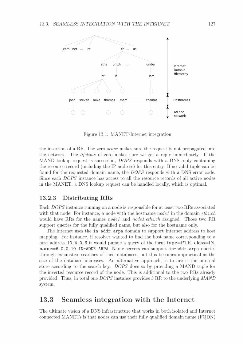
13.3. SEAMLESS INTEGRATION WITH THE INTERNET 127
Figure 13.1: MANET-Internet integration
the insertion of a RR. The zero scope makes sure the request is not propagated intothe network. The lifetime of zero makes sure we get a reply immediately. If theMAND lookup request is successful, DOPS responds with a DNS reply containingthe resource record (including the IP address) for this entry. If no valid tuple can befound for the requested domain name, the DOPS responds with a DNS error code.Since each DOPS instance has access to all the resource records of all active nodesin the MANET, a DNS lookup request can be handled locally, which is optimal.
13.2.3 Distributing RRs
Each DOPS instance running on a node is responsible for at least two RRs associatedwith that node. For instance, a node with the hostname node1 in the domain ethz.chwould have RRs for the names node1 and node1.ethz.ch assigned. Those two RRsupport queries for the fully qualified name, but also for the hostname only.
The Internet uses the in-addr.arpa domain to support Internet address to hostmapping. For instance, if resolver wanted to find the host name corresponding to ahost address 10.4.0.6 it would pursue a query of the form type=PTR, class=IN,name=6.0.0.10.IN-ADDR.ARPA. Name servers can support in-addr.arpa queriesthrough exhaustive searches of their databases, but this becomes impractical as thesize of the database increases. An alternative approach, is to invert the internalstore according to the search key. DOPS does so by providing a MAND tuple forthe inverted resource record of the node. This is additional to the two RRs alreadyprovided. Thus, in total one DOPS instance provides 3 RR to the underlying MANDsystem.
13.3 Seamless integration with the Internet
The ultimate vision of a DNS infrastructure that works in both isolated and Internetconnected MANETs is that nodes can use their fully qualified domain name (FQDN)

128 CHAPTER 13. DOPS: DOMAIN NAME AND PRESENCE SERVICE
transparently within the MANET as well as in the Internet. In other words, theonly change should be the scope of the corresponding domain name which will varydepending on whether the MANET is currently connected to the Internet or not. Forinstance, assume a node in the Internet with domain name node1.ethz.ch. Given thatthis node is temporarily detached from the Internet but attached a MANET, we wouldlike communication with other nodes in the MANET based on the node’s Internetdomain name (node1.ethz.ch) to be possible without applications to take notice. Onthe other hand, communication to and from the Internet should be possible as soonas the node gains Internet connectivity again.
13.3.1 Example
Imagine a scenario as illustrated in Figure 13.1. A research project involves severalresearch groups from different universities in Switzerland. Occasionally, the membersof the various groups will meet to discuss the latest state of the project. Duringthose meeting the people involved might want to exchange certain data related to thediscussion they have. However, rather than building a fixed network to exchange dataa MANET could be used. It would be important to have DNS infrastructure thatprovides the very same view on the network as if the nodes would be attached to theInternet. This would allow applications that exchange data to run in the MANET asif they would run in the Internet.
13.3.2 Query processing in Internet-connected MANETs
DOPS does not provide domain name resolution for nodes outside the ad hoc network.Rather, it forwards those DNS requests to the Internet. To implement the visionof transparent and seamless DNS connectivity, the DOPS system needs to decidewhether a node with a given domain name can be reached over the MANET or overthe Internet. There is no point in making such a decision if the DOPS instancereceiving the DNS request runs on a node without Internet access. If, however, anode is attached to both MANET and Internet2, things become more complicated.We refer to a node in this state as a hybrid node. One way to cope with hybridnodes would be to first forward the query to the Internet and trying resolve a namein the MANET only if the Internet query has previously failed. This creates anoverhead in the DNS response time while answering domain names that are currentlyonly reachable within the MANET. To cover the worst case, a timeout is neededto decide whether a given name can be resolved in the Internet or not. And evenif a DNS query sent to the Internet is successfully answered, it still does not tellanything about whether the given node is currently reachable through the Internet.Another possibility, the one implemented in DOPS, is to query the MANET first andonly in case of a failure trying to resolve a name in the Internet. The advantageis that querying the MANET in DOPS does not create any latency overhead sincethis corresponds just to a local lookup. One can argue that for nodes attached toboth Internet and MANET it would make more sense to respond with the IP addressthat belongs to the Internet since communication over the Internet typically is faster.There are two answers to this question. First, a MANET composed of nodes that are
2DOPS detects an Internet connection using the InternetDetectionAPI described in chapter 12

13.4. PERFORMANCE 129
Available Network ConnectionsDNS Configuration Query Type Ad Hoc Ad Hoc/Internet Internet
DOPS Ad Hoc 6.8ms 6.9ms 9.3msInternet 6.8ms 9.8ms 9.9ms
Regular DNS configuration Internet N/a N/a 10.1ms
Table 13.1: Average DNS response times taken from 10’000 measurements
at the same time attached to the Internet is not very common. Optimizing for thiscase would be suboptimal in many other cases which are far more likely (a MANETcomposed of nodes not attached to the Internet). The second answer is that wecan provide support for nodes that want to prioritize communication through theInternet. In DOPS this is done by configuring a separate domain name for usageonly in the MANET. A node may want to configure DOPS in such a way if the nodespends most of its time in a hybrid state communicating with other hybrid nodes.The separation of the domains gives priority to the communication over the Internet.The disadvantage is that the MANET-Internet integration under such a configurationis no longer transparent to upper layers.
13.4 Performance
We have evaluated DOPS both in real and by simulation. The performance metricswe studied are response time, update time and system agility (the ability to react tofrequent changes of the network under heavy load).
13.4.1 Response time
First we measured the response time of DOPS under different network settings. Themeasurements were done using 6 notebook computers running Debian 4.0. The lap-tops had a 2.0Ghz Mobile Pentium 4 and were equipped with an integrated 11Mbit/sIEEE 802.11a wireless network interface card. During some of the measurements, onelaptop was additionally attached to the Internet using a Gigabit Ethernet networkcard. Because it would be difficult to find a spatial separation of the notebooks whichwould have required multihop communication between them, an artificial separationusing packet filter rules was used: They were only allowed to communicate with theirdirect neighbors , all other traffic was dropped (by the default policy). All results areaveraged over a set of 10’000 tests.
The test settings differ in terms of whether the node submitting a DNS query isattached to the Internet access, or the ad hoc network, or to both the Internet andthe ad hoc network. Additionally, we distinguish the case where the domain name tobe resolved concerns a node in the ad hoc network, or a node in the Internet. Theformer is called a query of type Ad Hoc, the latter a query of type Internet.
From table 13.1 we see that resolving a domain name for a host in the ad hocnetwork, when being attached to the ad hoc network, takes 6.8ms on average. The

130 CHAPTER 13. DOPS: DOMAIN NAME AND PRESENCE SERVICE
response stays approximately the same (6.7ms) if the node additionally is attached tothe Internet. This is because in any case, DOPS first checks whether a given domainname can be resolved in the ad hoc network3. If a node tries to resolve a domain namefor a host that lies in the Internet, while the node itself is only attached to the ad hocnetwork, it takes as well around 6ms until a negative response is received. If, however,the node additionally is attached to the Internet, the domain name will successfullybe resolved with a response time of 9.8ms on average. This is because DOPS acts asa proxy and forwards the DNS query to the nameserver in the Internet. We madesome measurements to see what the overhead is of using DOPS for communicatingwith the Internet. We see that even if a node is solely attached to the Internet, anddetached from the ad hoc network, the average response time stays around 9.9ms,which is roughly the same as in the case where the node was additionally attachedto the ad hoc network. Therefore, the overhead of trying to resolve a domain namein the ad hoc network first is negligible. This is because looking up a domain namein the ad hoc network is only a local operation. We have also compared the responsetime for querying Internet host using DOPS versus sending DNS queries directlyto the Internet domain name server. From the Table 13.1 we see that the responsetime without using DOPS as a proxy stays approximately the same. Therefore,using DOPS will not cause any overhead when communicating with the Internet, butseamlessly integrates with the domain name system in the Internet.
13.4.2 Update time
The update time is the time it takes for DOPS to distribute a new resource recordfor a given domain name. This is important since it determines how fast the systemreacts when a new node joins the network or an existing node leaves the network.Since DOPS uses MAND to distribute the RRs across the network, the update timecorresponds to the tuple propagation shown in Figure 11.6 in chapter 11. Accord-ing to those figures, it takes around 0.8 seconds on average until its domain nameinformation is available to every node in the network, considering a network with 30nodes and a diameter of 5. Figure 11.9 further indicate that mobility has a positiveeffect on the update time.
13.4.3 Presence Detection
We have used ns− 2 to explore the behavior of DOPS in a larger scale. Our config-urations span from a basic configuration of 50 nodes deployed uniformly in an areaof 1500m × 300m, up to configurations with 100, 200, 500, and 1000 nodes spreadacross planes appropriately enlarged to maintain the aspect ratio and node density ofthe basic configuration. We carried out our experiments both over AODV and OLSRusing the same implementation we used already in chapter 11 to evaluate the MANDsystem.
In the first experiment we study the impact DOPS has on MAND when distribut-ing a large set of RRs/tuples. Remember that the MAND routing handler stores alltuples while they are waiting to be piggybacked onto an intercepted routing message.
3Note that this behavior can be changed in DOPS by configuring a special domain name for thenode to be used in the MANET
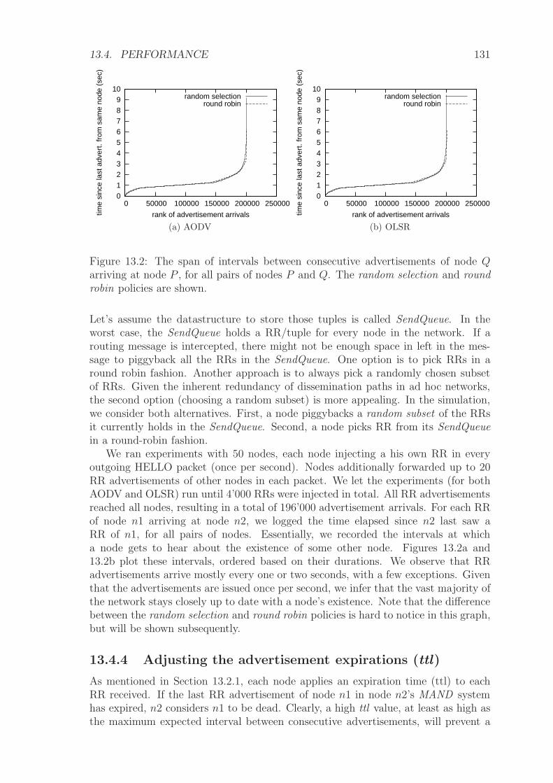
13.4. PERFORMANCE 131
0 1
2 3 4
5 6 7 8
9 10
0 50000 100000 150000 200000 250000
time
sinc
e la
st a
dver
t. fr
om s
ame
node
(se
c)
rank of advertisement arrivals
random selectionround robin
(a) AODV
0 1
2 3 4
5 6 7 8
9 10
0 50000 100000 150000 200000 250000
time
sinc
e la
st a
dver
t. fr
om s
ame
node
(se
c)
rank of advertisement arrivals
random selectionround robin
(b) OLSR
Figure 13.2: The span of intervals between consecutive advertisements of node Qarriving at node P , for all pairs of nodes P and Q. The random selection and roundrobin policies are shown.
Let’s assume the datastructure to store those tuples is called SendQueue. In theworst case, the SendQueue holds a RR/tuple for every node in the network. If arouting message is intercepted, there might not be enough space in left in the mes-sage to piggyback all the RRs in the SendQueue. One option is to pick RRs in around robin fashion. Another approach is to always pick a randomly chosen subsetof RRs. Given the inherent redundancy of dissemination paths in ad hoc networks,the second option (choosing a random subset) is more appealing. In the simulation,we consider both alternatives. First, a node piggybacks a random subset of the RRsit currently holds in the SendQueue. Second, a node picks RR from its SendQueuein a round-robin fashion.
We ran experiments with 50 nodes, each node injecting a his own RR in everyoutgoing HELLO packet (once per second). Nodes additionally forwarded up to 20RR advertisements of other nodes in each packet. We let the experiments (for bothAODV and OLSR) run until 4’000 RRs were injected in total. All RR advertisementsreached all nodes, resulting in a total of 196’000 advertisement arrivals. For each RRof node n1 arriving at node n2, we logged the time elapsed since n2 last saw aRR of n1, for all pairs of nodes. Essentially, we recorded the intervals at whicha node gets to hear about the existence of some other node. Figures 13.2a and13.2b plot these intervals, ordered based on their durations. We observe that RRadvertisements arrive mostly every one or two seconds, with a few exceptions. Giventhat the advertisements are issued once per second, we infer that the vast majority ofthe network stays closely up to date with a node’s existence. Note that the differencebetween the random selection and round robin policies is hard to notice in this graph,but will be shown subsequently.
13.4.4 Adjusting the advertisement expirations (ttl)
As mentioned in Section 13.2.1, each node applies an expiration time (ttl) to eachRR received. If the last RR advertisement of node n1 in node n2’s MAND systemhas expired, n2 considers n1 to be dead. Clearly, a high ttl value, at least as high asthe maximum expected interval between consecutive advertisements, will prevent a

132 CHAPTER 13. DOPS: DOMAIN NAME AND PRESENCE SERVICE
1e-05
0.0001
0.001
0.01
0.1
1
0 1 2 3 4 5 6 7 8 9 10
prob
abili
ty o
f fal
se n
egat
ive
ttl: duration a RR is kept on a node (sec)
random selectionround robin
(a) AODV
1e-05
0.0001
0.001
0.01
0.1
1
0 1 2 3 4 5 6 7 8 9 10
prob
abili
ty o
f fal
se n
egat
ive
ttl: duration a RR is kept on a node (sec)
random selectionround robin
(b) OLSR
Figure 13.3: The probability for a node to falsely consider another node dead (falsenegative), as a function of the ttl. Comparison between AODV and OLSR, andbetween random selection and round robin.
node from assuming another node dead due to some delay in its RR advertisement.On the other hand, with a very high ttl, dead nodes are remembered long after theirdeath and considered alive. Therefore, setting an appropriate value for ttl is a crucialtuning parameter of DOPS.
Figure 13.3 shows the probability of a node falsely considering another node tobe dead, as a function of the ttl, for a network of 50 nodes. The main observation isthat, irrespectively of the policy used, random selection or round robin, a ttl of lessthan 10 seconds can allow nodes infer other nodes’ death with accuracy. A secondobservation is that AODV and OLSR have the same behavior with respect to DOPSand RR advertisement updating.
Interestingly, round robin performs better than random selection. In random se-lection, some consecutive advertisements are delivered up to 8 seconds apart, whilein round robin the maximum interval observed between consecutive advertisementsis closer to 6 seconds. It is not hard to see why. Random selection picks the RRadvertisements to forward at random. This is asymptotically fair to all advertise-ments, but may lead in some temporal imbalance between the number a specific RRhas been forwarded in some neighborhood of the network. Round robin, on the otherhand, provides a much more predictable schedule in forwarding RRs, diminishing thethe worst case.
Finally, Figure 13.4 presents similar graphs for larger networks, or 100, 200, 500,and 1000 nodes. To avoid duplication of equivalent graphs, only AODV graphs areshown, but OLSR have been double-checked to appear the same. As expected, largernetworks impose higher delays in RR propagation, therefore a higher ttl value isneeded. For instance, for the case of 1000-node networks, nodes should be keepingadvertisement for at least 60 seconds to avoid falsely regarding other nodes as dead.However, if false negatives are not critical to the application using DOPS, a lower ttlvalue can be chosen, which will also allow the faster detection of dead nodes at thecost of some false accusations. In our example of the 100-node network, a ttl of 20seconds would allow nodes to detect dead nodes three times faster, at the cost that10% of the cases that a node is considered dead would be false.

13.5. RELATED WORK 133
1e-05
0.0001
0.001
0.01
0.1
1
0 2 4 6 8 10 12 14 16 18 20
prob
abili
ty o
f fal
se n
egat
ive
ttl: duration a RR is kept on a node (sec)
random selectionround robin
(a) 100 nodes
1e-05
0.0001
0.001
0.01
0.1
1
0 5 10 15 20 25 30 35 40
prob
abili
ty o
f fal
se n
egat
ive
ttl: duration a RR is kept on a node (sec)
random selectionround robin
(b) 200 nodes
1e-05
0.0001
0.001
0.01
0.1
1
0 10 20 30 40 50 60 70
prob
abili
ty o
f fal
se n
egat
ive
ttl: duration a RR is kept on a node (sec)
random selectionround robin
(c) 500 nodes
1e-05
0.0001
0.001
0.01
0.1
1
0 10 20 30 40 50 60 70 80 90 100
prob
abili
ty o
f fal
se n
egat
ive
ttl: duration a RR is kept on a node (sec)
random selectionround robin
(d) 1000 nodes
Figure 13.4: The probability for a node to falsely consider another node dead (falsenegative), as a function of the ttl. Simulations of larger networks
13.5 Related Work
A natural way of performing domain name resolution is to use a decentralized ap-proach in which a node of the MANET replies to a broadcasted name request for whichit is the target [155, 156, 157]. One problem with this approach is that it uses anexcessive amount of messages due the broadcasts triggered every time a domain nameneeds to be resolved. Broadcasting DNS queries is a particular waste of resources ifthe node matching the requested domain name is not present in the network. Anotherproblem is that resolving domain names on demand prolongs the overall communi-cation setup time (mainly consisting of the route establishment time). In [158, 159],the overall amount of messages as well as the communication setup time is loweredby integrating route discovery and domain name resolution. Another option is to usemulticast routing to propagate domain name mappings [160, 161]. However, all ofthose approaches are bound to one particular routing protocol, e.g., AODV [93] orDSR [122].
A number of solutions exist for providing DNS across the MANET-Internet bound-aries. In [159, 162], the authors propose a special domain net.lunar to be configuredat startup. An integrated DHCP server then appends the pre-configured domain toall nodes in the MANETs. In this way, the DNS system knows exactly which do-

134 CHAPTER 13. DOPS: DOMAIN NAME AND PRESENCE SERVICE
main it has to query the Internet for and which not. However, the method requiresapplications to communicate using the newly defined domain names. Moreover, twonodes respectively named john.domain1.net and john.domain2.com will both end upbeing identified inside the MANET as john.net.lunar.
Another approach, discussed in [125], is based on specialized gateway nodes whichforward DNS requests to the Internet and send back the replies. This approach,however, fails if the requested domain can be resolved in the Internet but the nodeis currently detached from the Internet but available in the MANET. As a solution,the authors propose to ping the node before returning the resolved address, but pingrequests are often blocked by firewalls. Alternatively, a DNS system could first tryto resolve the domain name in the MANET and try the Internet afterwards, butthis causes a huge overhead in response time when resolving domain names of nodeswhich are actively attached to the Internet.
13.6 Summary
In this chapter we have presented DOPS, a DNS and presence service for MANETs.DOPS is fully decentralized and at the same time seamlessly attaches to the Internetdomain name system. DOPS uses the MAND system for the distribution of DNSresource records. In this way, DOPS provides a novel but natural mechanism tocombine presence signaling and domain resolution with zero message overhead. Wehave shown that DOPS quickly reacts to network changes and provides a fast DNSresponse time.
Chapter 14
SIPHoc: Distributed SessionInitiation in MANETs
SIP is an important protocol and network service used by many applications in theInternet such as VoIP, video or chat. In this chapter, we present SIPHoc, a SIP com-patible middleware for session setup and management in MANETs. SIPHoc providesthe same interface as the SIP standard but its implementation is tailored to the de-centralized and dynamic nature of MANETs. Similar as DOPS for DNS, SIPHoc pro-vides SIP services beyond the MANET-Internet boundaries. We are testing SIPHocusing standard SIP-based VoIP applications to set up a VoIP communication betweennodes in the MANET and occasionally also nodes in the Internet.
14.1 SIP Overview
SIP works by building an overlay network on top of a regular IP network using a setof SIP entities such as proxies and registrar servers. A SIP proxy is an intermediaryentity primarily in charge of routing: its job is to ensure that a request is sent toanother entity ’closer’ to the targeted user. A SIP registrar is used by SIP applicationsto register their current location. A SIP location service is used by registrars to storeuser location information and by SIP proxies to query user location information.
A SIP application first registers with the system by communicating its SIP username and its current location to a registrar (Figure 14.1a). The registrar to be usedis either determined using DNS or it is statically configured (through the so calledoutbound-proxy). Registrars and proxies are logical entities and it is not uncommonto have them co-located on the same node. When the registrar hears from a node, itbuilds a binding, i.e., an association between a SIP user name and the correspondingcontact address (typically an IP address or resolvable name).
To establish a session with another user whose current location is unknown, a SIPINVITE message is sent to the proxy/registrar (step 1, Figure 14.1b). The proxyresponds with a 100 Trying message (step 2). The 100 Trying response indicatesthat the INVITE message has been received and that the proxy is trying to routethe INVITE message to the final destination. Since the outbound proxy/registrardoes not know the location of user B, it uses a DNS server to locate the proxy ofthe destination node and forwards the INVITE message accordingly (steps 3 to 6).The receiving proxy/registrar uses the previously registered binding information of
135

136CHAPTER 14. SIPHOC: DISTRIBUTED SESSION INITIATION IN MANETS
LocationService
3. 200 OK
User B:sip:[email protected]
2. Update DB
4. 2
00
OK
1. R
EG
ISTE
R
SIPProxy/Registrar
(a) SIP registration
DNSServer
LocationService
Media Data
5. INVITESIP
Proxy/Registrar
8. Response
User B:sip:[email protected]
9. IN
VIT
E
10. 1
80
Rin
gin
g
User A:sip:[email protected]
3. DNS Query 4. DNS Reply 7. Query
1. IN
VIT
E
6. 100 Trying
11. 180 Ringing
14. 200 OK
2. 1
00Tr
ying
12. 1
80R
ingi
ng
15. 2
00O
K
13. 2
00
OK
16. ACK
SIPProxy/Registrar
(b) SIP session setup
Figure 14.1: Basic SIP mechanism
the user to locate the destination (steps 7 and 8) and finally delivers the INVITEmessage to the intended recipient (step 9). The recipient responds with a 180 Ringingmessage, which is routed back through the two proxies in the reverse direction (step10 to 12). If user B decides to establish the session with user A, it responds witha 200 OK (step 13 to 15). Finally, user A sends an ACK message to confirm thereception of the 200 OK message (step 16). At this stage, the two users have learnedeach others’ contact address through the INVITE/200 OK messages and from thenon they communicate directly, bypassing the two proxies.
14.2 SIPHoc in MANETs
The basic principle of SIPHoc resembles the one of DOPS in that we run an instanceof a modified SIP proxy and registrar (SIPHoc proxy) on each node in the network1.
14.2.1 SIPHoc proxy
A standard SIP proxy/registrar accepts SIP registrations of a collection of users fromcertain domains. A SIPHoc proxy typically only accepts SIP registrations from users(applications) on that particular device. In addition to storing these registrationsin its local location service table, each SIPHoc proxy uses MAND to advertise itselfas the contact address for these registered users (e.g., as the outbound proxy forthose users). If a SIPHoc proxy receives an INVITE message and cannot find thetarget in its local location service table, it consults MAND and forwards the INVITEmessage to the proxy which was advertised as outbound proxy for this user (we callthis procedure dynamic outbound proxy selection).
An alternative approach would have been to implement a distributed storagesolution using MAND where each proxy knows the direct contact address of all otherSIP users in the MANET. Such a solution may look even more appealing but itcreates SIP incompatibilities. If each proxy can find out the location of the finaldestination of the session by itself (using MAND), SIP bindings are resolved directlyat the caller’s proxy and INVITE messages do not pass the callee’s proxy. This
1Again, a SIPHoc proxy may only run on nodes interested in participating a SIP service

14.2. SIPHOC IN MANETS 137
MAND
SIP Application SIP Application
SIP REGISTERsip:[email protected]
INVITEsip:[email protected]
SIP REGISTERsip:[email protected]
MAND PUT MAND PUTMAND GET
ProxyProxy
Alice Bob
SIP Incompatible
SIP Compatible
Figure 14.2: Operations of a SIPHoc proxy
violates the standard SIP message flow, where INVITE messages always pass theproxy where the target has registered in the first place. The modified message flowcreates problems with session mobility and session tear down.
In contrast to this, SIPHoc complies with the traditional SIP message flow. More-over, the use of a proxy at each device creates an infrastructure that is fully decen-tralized by design. Figure 14.2 illustrate both the message flow used by the SIPHocproxy (SIP compatible) as well as the message flow that creates SIP incompatibilities.
14.2.2 Example
How the SIPHoc proxy works can be best understood with an example. The examplemaps the standard SIP message flow shown in Figure 14.1. We assume two users Aliceand Bob. The IP addresses of the two machines of Alice and Bob are 192.168.220.1and 192.168.220.2 respectively. Each user runs a SIPHoc Proxy on port 5060 and aSIP application on port 5062. Both machines are in the MANET, within an arbitraryhop-distance from each other. ProxyA is the proxy used by Alice and ProxyB thatof Bob.
To register with SIPHoc, both users send their URI and contact address totheir proxies: sip:[email protected] and 192.168.220.1:5062 for Alice; sip:[email protected] and192.168.220.2:5062 for Bob. The local SIPHoc proxy for each user will then store thecorresponding entry in its local location service table. It will also insert a tuple intoMAND associating his contact address with the given user. The tuple inserted intoMAND by ProxyA on behalf of the registration of Alice may look as follows:
tuple
key=sip:[email protected],
value=192.168.220.1:5060,
lifetime=<sip-lifetime>,
scope=64
The lifetime of the tuple is inherited from the SIP lifetime that was specified inthe SIP registration message. Note that the entry in the local location service tablediffers from the entry sent to MAND in that the latter contains the contact addressof the proxy (port 5060) rather than the one of the user (port 5062). To establish

138CHAPTER 14. SIPHOC: DISTRIBUTED SESSION INITIATION IN MANETS
a SIPHoc session – assume Alice contacts Bob – Alice sends an INVITE messageto sip:[email protected] (9). ProxyA checks whether the target SIP URI is in the locallocation service table (10). If that is not case, it uses MAND to look up the correctoutbound proxy for the SIP URI (11-12). The tuple request issued to MAND maylook as follows:
request
key=sip:[email protected],
lifetime=0,
scope=64
The lifetime of zero makes sure a reply is sent immediately by MAND. As we will seelater (section 14.3, this is important when connected to the Internet. The scope of64 makes sure that, in case there is not matching tuple available locally, the requestis propagated to the network. Any valid tuple that is found in the network will notbe considered for the reply that is sent for this request, but it may be consideredfor the next request that received by MAND at a later point in time. Many SIPapplications, if they cannot establish a connection on the first attempt, will try fora second time after a timeout. In this case, MAND would have pre-fetched thecorresponding outbound-proxy information.
Once the outbound proxy for user sip:[email protected] is found, the INVITE messageis forwarded (13). There is no difference in whether a SIP proxy receives an IN-VITE message from the local user or from another proxy over the network. Hence,ProxyB, upon receiving the INVITE message, checks whether the requested SIP URIis available in its local location service table (14). In this case it will find the entry(registered by Bob as 192.168.220.2:5062), and can then forward the INVITE messageto Bob (15).
14.3 Internet-connected MANETs
In this section we enhance the architecture described in the previous Section to sup-port Internet connectivity. Similar as with DOPS, we are interested in a seamlessintegration of SIPHoc with the SIP infrastructure of the Internet. Clients of SIPHocshould use their officially registered SIP accounts2 transparently in the MANET.For instance, assume again a user Bob in the MANET with SIP URI sip:[email protected] that Bob’s SIP account is officially associated with the SIP provider at ethz.ch,we would like calls to and from the Internet to become possible as soon as the MANEThas Internet access. On the other hand, Bob should always be able to call any SIP userwithin the MANET – and vice versa – even if the MANET is currently disconnectedfrom the Internet.
We assume each SIPHoc instance to be in one of the following three states: ad-hoc,Internet, hybrid. In the adhoc state, where the only accessible network is theMANET, the SIPHoc proxy will operate as described in section 14.2. In the Inter-net state, where the only accessible network is the Internet, the proxy will act as aregular Internet-based SIP proxy. This means it will forward all the SIP messages to
2A SIP account associated with some official SIP provider in the Internet
14.4. CASE STUDY: VOIP IN MANETS 139
their appropriate next hop SIP target. For instance a SIP REGISTER message ofbob ([email protected]) would be forwarded to the SIP proxy that is responsible for thedomain ethz.ch. If the SIPHoc proxy is in the hybrid state, where it has access toboth the Internet and the MANET, the operation of the proxy is as follows. Besidesregistering users as described in section 14.2, the proxy now additionally forwardsSIP REGISTER messages to the Internet if a responsible proxy for the specified do-main is available. Upon receiving an INVITE message, the proxy contacts MAND tosee if an outbound-proxy is available in the MANET for the given SIP target. If nooutbound-proxy can be found, the INVITE message is forwarded to the Internet.
Typically, nodes with Internet access have multiple IP addresses assigned (seesection 12.3.2). Let’s call the IP address used in the MANET internal and theone used for communicating to the Internet external. SIP applications implementstatic binding, meaning that they use the IP address determined at startup timeto be included in the contact address field of any SIP message sent towards theproxy (REGISTER, INVITE). Since the external IP address might be configureddynamically at the time the node gains Internet access, SIP messages would carrycontact addresses pointing to an internal IP address. In practice, for connections toand from the Internet, one would however like to include the external IP address inthe contact header of the SIP message because these addresses are used later by theapplication to establish the actual session. To take care of this issue, the SIPHocproxy, upon receiving a SIP INVITE or REGISTER message, first saves the oldcontact address. It then changes the address in the SIP header of the message tomatch the external IP address. Once a response for a given request is received, thecontact address is changed back to the original address that is used by the local SIPapplication. This keeps the application totally unaware of whether it communicatesover the Internet or only within the MANET.
Figure 14.3 illustrates all the operations of the SIPHoc proxy described in thissection. The activities, highlighted grey and labeled ”Continue as usual”, refer to theprocedures described in section 14.2.
14.4 Case Study: VoIP in MANETs
Since SIPHoc is strictly SIP compatible, it allows out-of-the-box SIP based VoIP ap-plications to run transparently in MANETs. In this section we use Kphone as a VoIPapplication to evaluate our SIP infrastructure. However, we also have successfullytested SIPHoc with various other Softphones such as Linphone, Twinkle or Ekiga.From a user perspective, the metric of interest is the dial-to-ring delay, i.e., the timeelapsed between the caller clicking the button on the calling terminal and the timethe called party hears the ringing. This call setup includes a set of SIP messages(INVITE, TRYING, RINGING) as well as the associated routing messages and apotential overhead of MAND. Figure 14.4 illustrates all the messages and time inter-vals that contribute to the dial-to-ring delay of a SIP call. The duration of the callsetup depends on the current locations of caller and callee (MANET, Internet) andon the routing protocol used (AODV, OLSR). The following two sections evaluatethe session setup time for a) pure Ad Hoc environments and b) Internet-connectedAd Hoc networks.
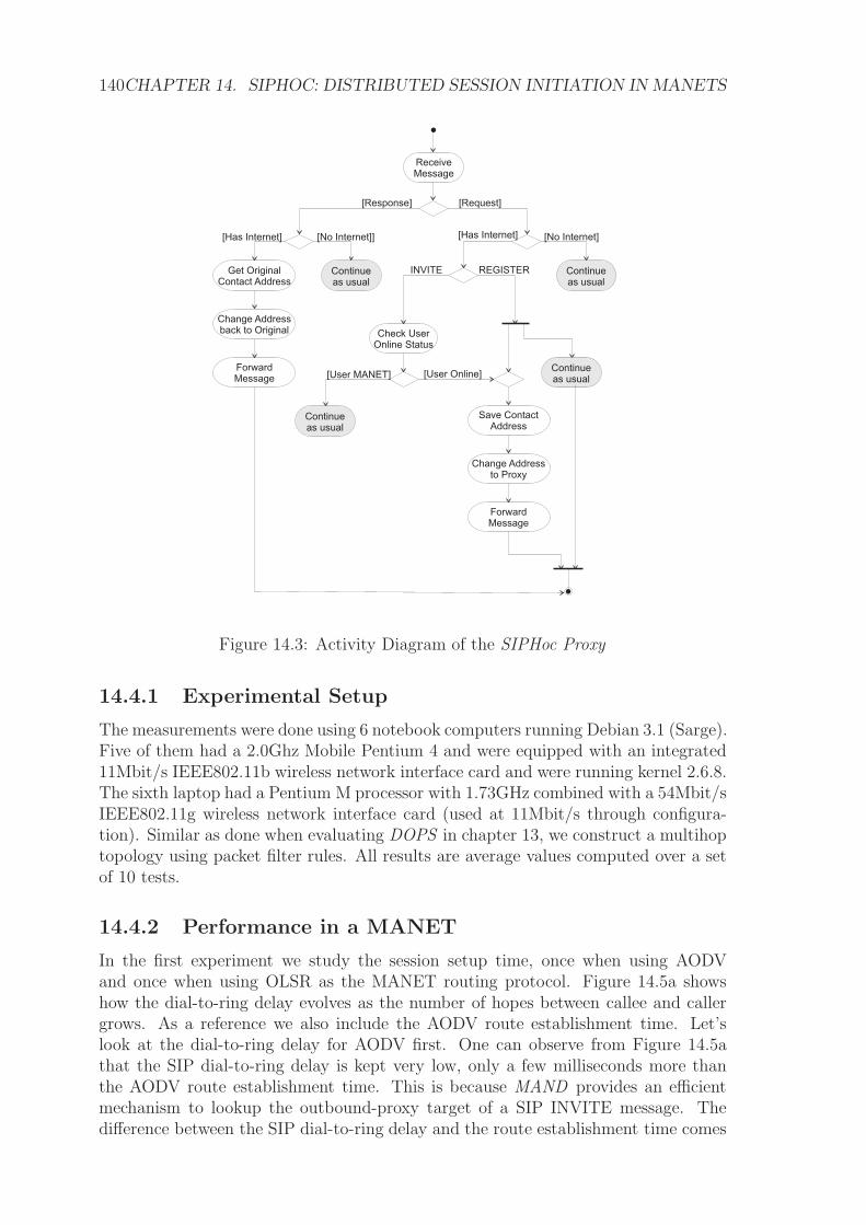
140CHAPTER 14. SIPHOC: DISTRIBUTED SESSION INITIATION IN MANETS
ReceiveMessage
Save ContactAddress
Continueas usual
[Response] [Request]
[No Internet][Has Internet]
Change Addressto Proxy
ForwardMessage
[No Internet]][Has Internet]
Continueas usual
Get OriginalContact Address
Change Addressback to Original
ForwardMessage
Check UserOnline Status
Continueas usual
[User MANET] [User Online]
INVITE REGISTER
Continueas usual
Figure 14.3: Activity Diagram of the SIPHoc Proxy
14.4.1 Experimental Setup
The measurements were done using 6 notebook computers running Debian 3.1 (Sarge).Five of them had a 2.0Ghz Mobile Pentium 4 and were equipped with an integrated11Mbit/s IEEE802.11b wireless network interface card and were running kernel 2.6.8.The sixth laptop had a Pentium M processor with 1.73GHz combined with a 54Mbit/sIEEE802.11g wireless network interface card (used at 11Mbit/s through configura-tion). Similar as done when evaluating DOPS in chapter 13, we construct a multihoptopology using packet filter rules. All results are average values computed over a setof 10 tests.
14.4.2 Performance in a MANET
In the first experiment we study the session setup time, once when using AODVand once when using OLSR as the MANET routing protocol. Figure 14.5a showshow the dial-to-ring delay evolves as the number of hopes between callee and callergrows. As a reference we also include the AODV route establishment time. Let’slook at the dial-to-ring delay for AODV first. One can observe from Figure 14.5athat the SIP dial-to-ring delay is kept very low, only a few milliseconds more thanthe AODV route establishment time. This is because MAND provides an efficientmechanism to lookup the outbound-proxy target of a SIP INVITE message. Thedifference between the SIP dial-to-ring delay and the route establishment time comes

14.4. CASE STUDY: VOIP IN MANETS 141
UserAgent A SIP Proxy MAND Routing
UserAgent BSIP ProxyMANDRouting
INVITE
100 TRYING100
TRYING INVITE
180RINGING
180 RINGING180RINGING
INVITE
GET
PiggybackTuple
OLSR Message ExtractTuple
PiggybackTuple
OLSR Message
Extract Tuple
REGISTER
REGISTER
PUT
Tuple
Node A Node BNetwork
Dia
l-to
-rin
g d
ela
yPUT
Regis
tration p
ropagation
Tuple
Pro
pagation
Figure 14.4: SIP registrations and call setup in a MANET using OLSR
0
0.1
0.2
0.3
0.4
0.5
0.5 1 1.5 2 2.5 3 3.5 4 4.5 5 5.5
AODVD2R AODVD2R OLSR
tim
e[s
ec]
distance in # hops(a) Ad Hoc Network
0
0.1
0.2
0.3
0.4
0.5
0 1 2 3 4 5 6 7 8 9
No routingAODVOLSR
tim
e[s
ec]
distance in # hops(b) Internet connected
Figure 14.5: Dial-to-ring delay
from the three additional messages involved in a SIP session setup (INVITE, Trying,RINGING). Thus the measurements prove that SIPHoc reduces the dial-to-ring delayalmost to the lowest value possible. The gap in time between three and four hopsin Figure 14.5a is due to AODV’s expanded ring search technique [93]. We haveexplained this phenomenon in section 11.5.5.
In contrast to the AODV case, the dial-to-ring delay for the OLSR case can bekept almost constant (around 0.1 seconds) and independent of the path length. Thisis because OLSR builds the routes in advance, before the SIP call takes place.

142CHAPTER 14. SIPHOC: DISTRIBUTED SESSION INITIATION IN MANETS
Internet
MANET
sip.ethz.ch
gateway
scenario 1 and 2
scenario 5, 6 and 7
scenario 3
scenario 4
Figure 14.6: Evaluation setup
14.4.3 Internet-connected environment: scenarios
The next experiment evaluates the dial-to-ring delay for Internet connections. Thesetup consists of 5 laptops3 arranged to form a linear 4-hop network. On the MANETside, there is user Alice with no direct Internet access. User Bob is on the otherextreme of the MANET and is on a node that – in some experiments – acts asgateway and has Internet access. A third user, Chris, is located in the Internet. Wealso assume a SIP proxy on sip.ethz.ch located in the Internet. We have evaluatedthe dial-to-ring delay in 7 scenarios as illustrated in Figure 14.6: (1) Bob callingChris using an unmodified out-of-the-box SIP proxy4 as a forwarding proxy for Bob;(2) Bob calling Chris using SIPHoc; (3) Alice calling Chris using Bob as a gateway;(4) Chris calling Alice using Bob as a gateway; (5) Bob calling Alice when Bob isdisconnected from the Internet; (6) Bob calling Alice when Bob is connected to theInternet; and (7) Bob calling Alice when Bob is connected to the Internet and Alice isconnected to the Internet using the gateway provided by Bob (therefore the INVITEmessage is routed through the Internet). We also include the cost of an AODV routerequest (8) for comparison.
14.4.4 Internet-connected environment: experiments
Each set of bars in Figure 14.5b corresponds to the result of one scenario, with thex-axis representing the scenario identifier. For all scenarios except the first one, weconsider both the case where AODV is used as a routing protocol and the case whereOLSR is used.
Scenarios 1 and 2 are SIP connections over the Internet. They allow to determinethe cost of SIPHoc over a plain SIP infrastructure. The results show that the over-head of SIPHoc (scenario 2) is small compared with the cost of using a plain SIPproxy (scenario 1). The overhead comes from the SIPHoc Proxy that performs vari-ous checks (looking up whether the node has Internet connection or not, contacting
3DELL Latitude, 2Ghz Intel Pentium IV, 256 MB RAM4We have used the JAIN Proxy: http://snad.ncsl.nist.gov/proj/iptel

14.5. RELATED WORK 143
MAND) before forwarding the actual INVITE message to sip.ethz.ch. Thus, there isno difference between the dial-to-ring delay for AODV and OLSR in scenario 2.
Scenarios 3 and 4 are in the range of scenario 2 indicating that the 4-hop la-tency in the MANET is rather negligible compared to the whole session setup time.Furthermore, scenarios 3 and 4 confirm that both directions, MANET-Internet andInternet-MANET, perform similarly. The reason why there is no significant differ-ence between the AODV and the OLSR case is that the route between Alice and thegateway has been established during the gateway discovery phase which took placeasynchronously in a separate process (connection provider, Section 12.3.2) before theactual session establishment.
In scenario 5, the target user resides in the ad hoc network. If AODV is used, aroute from Bob to Alice has to be established on demand which increases the dial-to-ring delay. One can observe that the overhead indeed is in the range of an AODVroute establishment (scenario 8). If OLSR is used no route establishment overheadis observed due to the pro-active behavior of OLSR.Scenario 6 leads to a similar result as scenario 5. Although Bob is connected to theInternet in scenario 6 the SIPHoc proxy is routing the SIP INVITE message directlytowards the outbound-proxy it has discovered using MAND.
In scenario 7 both users Alice and Bob are connected to the Internet. However,the SIPHoc proxy always first contacts MAND for a potential outbound-proxy, thusrouting the SIP INVITE message through the ad hoc network which results in asimilar performance as scenario 5 and 6.
The results have shown that the overhead for calls to and from the Internet iswithin an acceptable range. This is mainly because outbound-proxy information forall users in the network are distributed pro-actively using MAND. Thus, decidingwhether a given user is available in the ad hoc network or not comes at almost nocost.
14.5 Related Work
The Session Initiation Protocol SIP is a protocol set up a media session between twopeers in the Internet. It is used most commonly in applications such as VoIP, videoor chat. In a MANET, SIP must operate in a fully distributed manner while main-taining the same interface and procedures. This is a challenge because several of theproblems caused by the decentralized nature of MANETS can be solved by ignoringSIP procedures. For instance, registrars can be eliminated if all applications pro-actively announce their contact addresses. This can be done using either a HELLOmethod [163] or REGISTER broadcast messages [164]. Such approaches create a sig-nificant message overhead and introduces incompatibilities with session mobility andtear-down. As an optimization, [164] suggests to use the Service Location Protocol(SLP) [133] to discover the SIP bindings. Unfortunately, SLP is also centralized andvery inefficient in MANETs due to the heavy use of multicast [165]. Existing workto make SLP more efficient in MANETs is highly routing protocol specific [166].
SIP relies on DNS to locate nodes. A way to bypass the lack of a DNS infrastruc-ture in MANETs is to restrict the network topology and assign specialized roles togiven nodes [167]. This approach makes the endpoint discovery process easier andeliminates the need for (part of) the registrar since the position and communication
144CHAPTER 14. SIPHOC: DISTRIBUTED SESSION INITIATION IN MANETS
paths to all nodes are known in advance. This approach does not introduce messageoverhead but imposes strong restrictions on the routing protocols. It is also verydifficult to efficiently maintain a fixed routing topology in mobile settings.
Connecting the SIP-based applications to the Internet poses several problems.First, the SIP proxy does not know whether the target node is in the MANET oroutside. Second, establishing sessions between nodes in and outside the MANETrequires stable IP addresses. This can be done by using NAT [168] but it also requiresadditional mechanism like STUN [153]. If no NAT is available, extra mechanisms areneeded to maintain consistent network addresses across connections of the MANET tothe Internet. A way to avoid such problems is to assume the MANET is permanentlyconnected to the Internet. Then one can impose a fixed network topology leadingto the gateway [169]. This approach does not work for establishing SIP sessionsin MANETs not connected to the Internet and re-introduces the problems of fixedtopologies.
14.6 Summary
In this chapter we have presented SIPHoc, a middleware providing SIP-compatiblesession establishment in both isolated and Internet-connected MANETs. Our ex-periments illustrate that SIPHoc is able to establish sessions within a few hundredmilliseconds, regardless whether the other party is located in the MANET or in theInternet. Due to the efficient architecture of SIPHoc, the overhead in the dial-to-ringdelay stays in the order of a route discovery time, which is the lowest value possiblesince the cost of a route discovery has to be paid anyway.

Chapter 15
Network services in MANETs: ADiscussion
The network services described in the previous chapters share some important designprinciples and system properties. We want to briefly highlight those and reflect abouttheir impact onto different quality metrics of the system.
1. Proxy architecture: In a MANET, network services must operate in a dis-tributed manner while maintaining compatibility with the standard they are im-plementing. We adopted a proxy-based approach to meet both requirements.The basic concept is to run a proxy of a given service on each node in theMANET and share common objects (such as, e.g., contact information of SIPusers) using MAND. The local proxy makes it possible to transparently hidethe distributed implementation from the standard interface provided to upperlayers.
2. Piggybacking: Turning a centralized or hierarchical network service into a dis-tributed service for MANETs requires distributing service data across the net-work. MANETs are known to have only limited throughput capacity. Throughthe use of routing message piggybacking we were able to come up with a solutionthat is highly message efficient.
3. Pro-active: Applications like chat or VoIP may send many DNS or SIP re-quests during a regular session. The response time of those requests directlydetermines how fast those applications can react to user events, such as, sessionestablishment or message exchange. Thus, a fast response time must be an im-portant criteria for new service architectures considering that communicationdelays in MANETs are already high compared to, e.g., the Internet. All ourservices implement a pro-active distribution of service data. By doing so, agiven service is able to respond immediately to a request by consulting his localcache. This is of particular importance when interacting with the Internet. Iflocal information can used to determine whether a given service can be providedin the MANET or not, a network service will be able to immediately forward arequest to the Internet without noticeable overhead.
4. Lazy distribution: Typically, pro-active approaches have been shown to bemessage inefficient. This is true for instance in terms of routing. We already
145

146 CHAPTER 15. NETWORK SERVICES IN MANETS: A DISCUSSION
discussed the fact that our services use message piggybacking to avoid additionaltraffic load. However, what saves all those extra messages is not only thepiggybacking, but also the fact that service data is sent lazy. That way we areable to multiplex various service data of different services onto one single packet.Lazy data distribution has been shown to be very efficient also in other fieldsof research. For instance, it has been shown that a delay-tolerant mechanismto exchange packets in wireless networks can lead to a significant improvementin throughput capacity [170]. In the field of database replication, lazy datasynchronization has successfully been used to decrease the transaction responsetime [171].
5. Reliability: Network services such as DNS or SIP have to operate as reliable aspossible. The limiting factor thereby is the network itself. In the Internet, thenetwork is supposed to be reliable, thus service access is possible all the time.In a MANET, the network is inherently unreliable. The wireless signal is errorprone and packet loss is a common observation. Those problems induce furtherdifficulties on higher layers such as routing. Routing is an essential componentof the IP layer which all the network services described in this thesis are basedon. Failing to establish a route between to IP endpoints makes it impossible toaccess a given service remotely. Thus, routing constitutes the limiting factor forall network services in MANETs. By piggybacking service data onto routingmessages, we interlink the service data availability with the ability to access aservice. Or in other words, if the service data is not available to the service,then this is because there is currently no route between the producer and therequester of the service data.
6. Memory consumption: Some of the network services we presented implementfull replication of service data. Therefore, one issue to be considered is memoryconsumption. In DOPS the information that is stored on each node is thedomain names and the IP addresses of each of the other nodes in the network.Since each node typically has only one wireless interface with a configuredhostname assigned, the amount of data to be stored at each node is a linearfunction of the total number of nodes in the network. If we assume a directorymapping (domain name, IP address) can be stored using, on average, 50 bytes(4 bytes for the IP address and 46 bytes for the domain name), 25K of memorywould be sufficient to support a network of 500 nodes. In the case of SIPHoc,we can assume a similar upper bound for the memory consumption since it isunrealistic to have more than one active SIP account per node. For MANET-SLP the amount of memory needed grows linearly with the number of servicesthat are registered. There might be more than one service per node. The onlyway to handle this issue is to define an upper limit on the total number ofservices that can be registered on one single node.
Most systems dealing with storing and looking up data have to deal with tradeoffsamong several properties, like response time, update time, consistency, memory space,etc. In most cases it is impossible to build win-win systems, for instance providing fastresponse and update times, offering high consistency, and consuming less memory.When building a system, one has to optimize for a subset of these properties. Whichproperties to optimize for depends on the characteristics of the system (e.g., the ratio

147
between queries and updates) and the context in which the system is supposed torun. The decision made in this thesis, when designing the various network services,were influenced by the intrinsic properties of MANETs. Some of those properties,like connectivity or throughput capacity, have been studied in the first part of thisthesis.

148 CHAPTER 15. NETWORK SERVICES IN MANETS: A DISCUSSION

Chapter 16
Social Ad Hoc Networking
As a fourth an final demonstrator of MAND we present in this chapter AdSocial,a social networking application for MANETs. AdSocial allows nearby users in theMANET to interact spontaneously by exchanging profile information or by openinga chat or VoIP conversation. We have deployed AdSocial on a testbed of 23 handhelddevices and tested it during various group activities.
16.1 Overview
People use social networks to exchange information, images, video clips or to justcommunicate common interests. In contrast to many sites providing this kind of in-teraction over the Internet, like Facebook, ICQ, etc., AdSocial runs on MANETs. Thekey difference between AdSocial and traditional social networks lies in the way userscommunicate with each other. In Internet-based social applications users communi-cate with so called friends (other previously contacted users). In AdSocial, interactiontakes place between nearby users in the ad hoc network, so called buddies. An adhoc network might emerge temporarily in everyday’s life or during business, e.g., onthe train when travelling to work, at a conference or during a business meeting. AnAdSocial user can create a profile in which he/she specifies interests and other per-sonal information. AdSocial signals the user’s presence in the ad hoc network usingMAND. The users in the ad hoc network can retrieve the profile of their buddies aswell as search for nearby buddies with specific interests. Moreover, AdSocial providesthe basis for running collaborative applications. For instance, AdSocial integrateswith existing VoIP or chat applications on the device. If a profile of a user contains aSIP VoIP address or a chat address, AdSocial will immediately start a VoIP or chatsession with the given person. In all those cases, AdSocial is used as a first step toget in contact with people around each other.
16.2 Architecture
AdSocial runs as a local web application in a regular browser. The various compo-nents involved on one single node in the ad hoc network are illustrated in Figure16.1. The local browser connects to the web server that redirects the call to the Ad-Social application via a FastCGI interface [172]. Depending on the state of the webapplication AdSocial serves static files containing the presentation logic or gathered
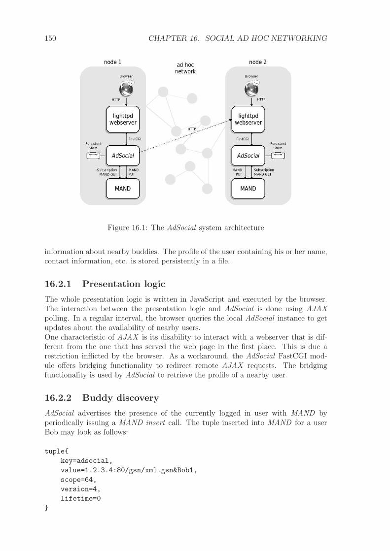
150 CHAPTER 16. SOCIAL AD HOC NETWORKING
Figure 16.1: The AdSocial system architecture
information about nearby buddies. The profile of the user containing his or her name,contact information, etc. is stored persistently in a file.
16.2.1 Presentation logic
The whole presentation logic is written in JavaScript and executed by the browser.The interaction between the presentation logic and AdSocial is done using AJAXpolling. In a regular interval, the browser queries the local AdSocial instance to getupdates about the availability of nearby users.One characteristic of AJAX is its disability to interact with a webserver that is dif-ferent from the one that has served the web page in the first place. This is due arestriction inflicted by the browser. As a workaround, the AdSocial FastCGI mod-ule offers bridging functionality to redirect remote AJAX requests. The bridgingfunctionality is used by AdSocial to retrieve the profile of a nearby user.
16.2.2 Buddy discovery
AdSocial advertises the presence of the currently logged in user with MAND byperiodically issuing a MAND insert call. The tuple inserted into MAND for a userBob may look as follows:
tuple
key=adsocial,
value=1.2.3.4:80/gsn/xml.gsn&Bob1,
scope=64,
version=4,
lifetime=0
16.3. DEPLOYMENT 151
The value of the tuple contains information about the IP address of local node, theport where the webserver is running, the absolute path to the XML engine on localweb server, the actual nickname of the user and its availability status. The availabilitystatus is specified by the user and corresponds to either available (1), busy (2) oraway (2). Tuples describing user presence information are issued with a lifetime ofzero and a large scope. Tuples of this form can be seen as events notifying remoteapplications with open subscriptions for the common event/tuple key (”adsocial”).Other examples of MAND events are given in chapter 12 (SLP) and in Figure 11.3.
Users in the context of a list of friends are often referred to as ”buddies”. The listof buddies of a user is maintained by AdSocial based on the MAND events it receives.In order for AdSocial to receive all events containing buddy presence information itwill periodically issue a MAND lookup call (see section 11.4 for details).
request
key=adsocial,
scope=0,
version=0,
lifetime=60
16.2.3 VoIP and video: integration with other applications
One of the most exciting features of AdSocial is that it integrates very well with othercollaborative applications. Since the user interface runs in a browser, the browsercan be configured to perform an associated action for a specific file type. We haveleveraged this feature to interlink AdSocial with VoIP and video applications using ourSIPHoc infrastructure. Each device running AdSocial will additionally have SIPHocand a VoIP client installed. If a user retrieves a profile of another nearby buddy, andthe profile contains the SIP address of the buddy, he/she will be able to open a VoIPsession by just clicking on the SIP address within the profile.
Similarly as for VoIP and video, one could also configure the browser to interlinkAdSocial with an instant messenger. However, AdSoical already integrates a simplechat application to support chat among buddies in the ad hoc network.
16.3 Deployment
AdSocial was designed and implemented for Linux, as all other systems that have beenpresented in this thesis. Since AdSocial is supposed to be a pervasive application it isimportant to deploy it on devices people can carry with them in their everyday life.We have deployed AdSocial on Nokia Internet Tablets [173]. Those devices run Linux(Maemo Linux [174]), are small enough to be carried around and they are equippedwith a WLAN card that can be switched into ad hoc mode. The upper part of Figure16.2 shows two Nokia N800 Internet tables with AdSocial running. The figures showthe user profiles of two users, Patrick and Oriana. The left hand side of the profilescontains personal information of the users, such as a photo, his or here interests orthe SIP address. On the right hand side the nearby buddies are displayed. Users canretrieve the profile of nearby buddies by right-clicking on the buddy’s icon. Similarly,they can also open a chat session with a buddy.

152 CHAPTER 16. SOCIAL AD HOC NETWORKING
Figure 16.2: AdSocial: social networking among Nokia N810 devices
Each Nokia device by default comes with a VoIP and video application. Moreover,the standard web browser on the devices is already configured to use the VoIP/videoapplication when opening SIP URL’s. Hence, AdSocial users on the Nokia devicesthat have their SIP address specified in their profile can easily initiate VoIP or videoconversations among themselves by clicking on other user’s SIP address. A picture ofa phone conversation between two users in the ad hoc network is shown in the lowerleft corner of Figure 16.2. What cannot be seen from the picture is that the VoIPapplication displays “Internet call” whenever a call is coming in from another userin the ad hoc network. This once more demonstrates that SIPHoc is SIP compatibleletting SIP applications believe that they are communication across the Internet,while they are actually communication over an ad hoc network.
Experiments with social applications require a minimum amount of users to par-ticipate. Nokia kindly provided us with 20 N810 devices to be used for larger exper-iments. A picture of all devices is shown in the right corner of Figure 16.2.
16.4 Measurements
AdSocial was tested during the Retreat 2008 of the ETH Systems group, held inArosa, a small town in the mountains of Switzerland. The event brought together 34members of the group for three days in total. Our testbed consists of 18 Nokia N810Internet tables, which have been distributed among the attendants of the event. Wehave used OLSR as the MANET routing protocol since earlier tests have shown thatOLSR performs better than AODV in terms of route stability and route recovery.
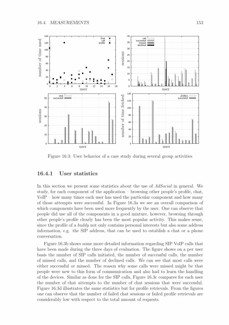
16.4. MEASUREMENTS 153
0
20
40
60
80
100
120
140
0 2 4 6 8 10 12 14 16 18
chatcall
profile
user
num
ber
oftim
euse
d
0
5
10
15
20
25
30
35
40call
succesfullmissed
declined
user
sess
ions
0
10
20
30
40
50chat
succesfull
user
sess
ions
0
20
40
60
80
100
120
140profiles
succesfull
user
num
ber
oftim
efe
tched
Figure 16.3: User behavior of a case study during several group activities
16.4.1 User statistics
In this section we present some statistics about the use of AdSocial in general. Westudy, for each component of the application – browsing other people’s profile, chat,VoIP – how many times each user has used the particular component and how manyof those attempts were successful. In Figure 16.3a we see an overall comparison ofwhich components have been used more frequently by the user. One can observe thatpeople did use all of the components in a good mixture, however, browsing throughother people’s profile clearly has been the most popular activity. This makes sense,since the profile of a buddy not only contains personal interests but also some addressinformation, e.g. the SIP address, that can be used to establish a chat or a phoneconversation.
Figure 16.3b shows some more detailed information regarding SIP VoIP calls thathave been made during the three days of evaluation. The figure shows on a per userbasis the number of SIP calls initiated, the number of successful calls, the numberof missed calls, and the number of declined calls. We can see that most calls wereeither successful or missed. The reason why some calls were missed might be thatpeople were new to this form of communication and also had to learn the handlingof the devices. Similar as done for the SIP calls, Figure 16.3c compares for each userthe number of chat attempts to the number of chat sessions that were successful.Figure 16.3d illustrates the same statistics but for profile retrievals. From the figuresone can observe that the number of failed chat sessions or failed profile retrievals areconsiderably low with respect to the total amount of requests.

154 CHAPTER 16. SOCIAL AD HOC NETWORKING
0
200
400
600
800
1000
1200
1400
tim
e[s
ec]
calls
Figure 16.4: SIP call durations
0
5
10
15
20
time [sec]
nei
ghbor
s/buddie
s/tu
ple
s
neighborsbuddies
MAND tuples
Figure 16.5: SIP call durations and buddies/neighbors/tuples vs time
16.4.2 VoIP statistics
As illustrated in Figure 16.2a, during the three days of evaluation people made ex-tensive use of the VoIP and video applications which are interlinked with AdSocialthrough the browser (Section 16.2.3). Figure 16.4 shows the durations of each callmade. Every point in Figure 16.4 corresponds to a phone conversation with its y-value describing the duration of the call measured in seconds. As can be observed,most phone calls lasted less than 100 seconds, however, there are also some calls witha duration of more than 16 minutes. It’s very likely that the long calls were actuallyvideo conversations where the devices were used like a web-cam and were not movedfor most of the time.
In Figure 16.5 we study different properties related to AdSocial, SIPHoc andMAND. The Figure shows the overall correlation between all the SIP tuples, numberof AdSocial buddies, and number of neighbors in the routing table. The graph hasbeen derived from the log files of one device over a period between 12:45 and 15:30,which is a period when most devices were in frequent use. The graph shows that thevariation of the number of neighbors is much higher than the variation of the numberof buddies, which is still higher than the variation of the number of SIP tuples. Thefact that the reactivity of MAND does not entirely map the constant fluctuations inthe routing table is due to the lifetimes of the tuples. Remember that tuples have a

16.4. MEASUREMENTS 155
specified lifetime for which they are guaranteed to stay in the system, even if theyare not refreshed. Thus, a tuple may still be in the system although the node thatoriginally generated the tuple has already left the network. From the Figure we alsoobserve that if the number of buddies change over a longer period of time, the tuplesin the MAND system will change accordingly.
There is no project that addresses social networks in MANETs. But there aresome social network related approaches that are worth mentioning. The Internetcompany Google is about to define a standard for storing, retrieving and processinguser related data in social networks. The project is called OpenSocial [175] and isstill in alpha state. It mainly describes a JavaScript API for manipulating profiledata. With the interface it will be possible to create new services using the existinginfrastructure of an social network provider. The problem up to now is that OpenSo-cial is only a collection of functions that a social network provider should implementsto allow the community to grow with the ideas of its members. Letting the memberenhance the functionality of the service. There is no reference implementation andthe definitions of what the functions should do are sufficiently general that no finalimplementation has been derived so far.
The OpenID Foundation provides a mechanism to maintain a user profile in acentral place and powering other sites using such data with the deposited information.The project is called OpenID [176]. Whenever a user joins a message board or acommunity site he or she has to state certain data, mainly contact information likename and e-mail address. But this has to be done for each such site over and overagain. OpenID collects this data once. Then the user can join the OpenID enabledcommunity and the required data is transmitted to the site. The user only needs toallow the community server to access his or her profile. OpenID allows to maintainthe profile in one central place, but also updates and changes to the profile canbe delegated to the connected community sites depending on their implementation.OpenID also permits the social network applications to collect data locally. They arenot forced to request the data again. This is why the update mechanism may fail.But sites that use OpenID for more than just a login replacement should take careof that.
During the last years most research addressing ”ad hoc” and ”social networks”has been targeting the development of appropriate models to simulate mobility [177]in MANETs. Heavy load and behaviour is tested not in real life but with simulations.Thus analysis that model that and other interesting behaviour [178] more accuratelywere and are developed. In the past many such models evolved because of findingsbased on small world [179] observations of MANETs. Thus the models may have beentoo optimistic, because the small world phenomena does not apply to all wirelessnetworks. But it may still be realistic, because social networks tend to be not asgeneral as ad hoc networks could be [180].
There is a trend to port existing social network ideas to mobile phone archi-tectures. Depending on the approach they use the web to access contents or runentirely message based. Mobikade [181] is a Web based free mobile social networkingservice (SNS) aiming to bring the massive success of Japanese mobile SNS sites toEurope. It differentiates from other social networking sites by the fact that it is anexclusively mobile based community and accessible only through the mobile phone.Dodgeball [182] is an SMS based social networking software provider for mobile de-vices. Users text their location to the service, which then notifies them of crushes,
156 CHAPTER 16. SOCIAL AD HOC NETWORKING
friends, friends’ friends and interesting venues nearby. Many others like Zingku, Rab-ble, Moblabber, Wadja, Zemble, twitter, etc. work all similarly. More or less theyare just group messaging systems for mobile phones with some additional features.
There are some implementations of social network applications that work on mo-bile phones and other portable devices that are not message or web based, but theymainly use bluetooth to communicate. Some examples are MobiLuck, ProxiDating,CrowdSurfer. There is also a relatively new application that uses a wireless LANconnection between the devices to detect nearby users. It is called Jambo Networks.Jambo is also a group communication tool that will detect members of the samegroup or groups the current user is participating. It is also possible to search forpeople in the area and contact them.
16.5 Summary
In this chapter we presented the design and implementation of a social networkingapplication that addresses the issues of MANETs. Users are able to create profilesdescribing their interests and contact information, search for other users with similarinterests and even to directly contact each other with the small built in chat applica-tion. Moreover, AdSocial integrates MANET VoIP and allows users to seamlessly setup a phone call among each other. We have deployed AdSocial on Nokia N800 hand-held devices and evaluated the application during a group activity in the mountainsof Switzerland.

Chapter 17
Conclusion
Mobile Ad Hoc Networks have not yet become reality. Most of the deploymentsare either of very small scale or they are part of academic research projects. Theproblems to be solved for MANETs to enter real life are of various forms. In this dis-sertation we have addressed two sets of problems which we consider to be particularlyimportant. In the first part of the thesis we have studied fundamental properties ofad hoc networks. We followed a numerical approach based on Monte-Carlo methodswhich allowed us to put a strong emphasize on realistic physical layer models. Asone example, we showed how network connectivity and throughput capacity evolvesunder log-normal shadowing radio propagation. Our results illustrate that the radioirregularity induced by log-normal shadowing has indeed a beneficial impact on con-nectivity and throughput capacity. This is of interest since it shows that an analysisof connectivity and interference in a circular radio propagation model yields worstcase bounds for both connectivity and interference. Until now, the assumption thatshadowing increases interference led to assuming that a circular radio propagationrange was a best case scenario for network capacity. As part of our effort to considerrealistic network models we have further studied the impact of different interferencemodels on throughput capacity. It was shown that there is a significant gap betweenthroughput capacity under the protocol model versus under the physical model. Thisis of importance since the protocol model served as the basis for many analytical re-sults on capacity and interference. In the last chapter of part I we have extended ourapproach on throughput capacity to study bandwidth reservation in ad hoc networks.More precisely, we show that there is an inherent trade-off between the quality of abandwidth reservation and the amount of resources wasted due to over-reservations.The quality of the reservation deteriorates even more when considering irregular radiopropagation. Overall, the first part of this thesis presents interesting new insight intothe behavior of fundamental properties of ad hoc networks under realistic physicallayer models and finite network boundaries. Taken together, the results may help toassess and design real network deployments.
In the second part, we considered ad hoc networks from a system’s research per-spective. We have presented several network abstractions and services that facilitatethe seamless transfer of standard IP-based applications to MANETs. The virtualinterface described in chapter 10 allows nodes with different media access technolo-gies to form one single IP based mobile ad hoc network. In such a network, routing,packet forwarding and mobility support take place independent of whatever wirelessaccess technology is used on a device. We belief that our approach of virtualizing
157
158 CHAPTER 17. CONCLUSION
the communication layer not only provides an efficient solution to integrate hetero-geneous classes of devices and network stacks, but is also an important technique tobuild any form of distributed service in MANETs. We have presented in chapters12, 13 and 14 distributed SLP, DNS and SIP services, each of them appearing asone virtual network service to the application layer. Those services allow standardInternet-based applications like, e.g., VoIP or chat, to run in MANETs without needof any modification. Moreover, the network services integrate seamlessly with theInternet and therefore provide applications with the possibility to communicate toand from the Internet whenever one node in the MANET has Internet access. Thecore part of the services presented in this thesis relies on MAND (chapter 11), anefficient distributed key/value store. MAND is message efficient since the distribu-tion of key/value information is solely based by piggybacking onto routing messages,traffic that is sent anyway. As a fourth and final demonstrator of MAND, we pre-sented a novel social networking application for MANETs. AdSocial allows to browsepersonal profiles of nearby users and provides abilities open a chat or VoIP session incase there is interest. All of the systems presented in part II of the thesis have beendeployed on Nokia N800 handheld devices and approved by real experiments. Over-all, the second part of this thesis demonstrates how a middleware based approachcan be used to build a transparent platform for existing networking applications tobe run in MANETs. In this regard, our approach can be seen as a new paradigm fordistributed systems in MANETs, in contrast to former approaches where dedicatedapplications have been considered to be the solution to cope with the complexity ofMANETs.

Bibliography
[1] Y.-C. Cheng and T.G. Robertazzi. Critical connectivity phenomena in multi-hop radio models. Communications, IEEE Transactions on, 37(7):770–777, Jul1989. ISSN 0090-6778. doi: 10.1109/26.31170.
[2] P. Gupta and P. Kumar. Critical power for asymptotic connectivity in wirelessnetworks. Stochastic Analysis, Control, Optimization and Applications, 1998.
[3] O. Dousse and P. Thiran. Connectivity vs capacity in dense ad hoc net-works. In O. Dousse and P. Thiran, Connectivity vs capacity in dense adhoc networks, in Proc. of IEEE INFOCOM, Hong Kong, 2004., 2004. URLciteseer.ist.psu.edu/dousse04connectivity.html.
[4] O. Dousse, P. Thiran, and M. Hasler. Connectivity in ad-hoc and hybridnetworks. INFOCOM 2002. Twenty-First Annual Joint Conference of theIEEE Computer and Communications Societies. Proceedings. IEEE, 2:1079–1088 vol.2, 2002. ISSN 0743-166X. doi: 10.1109/INFCOM.2002.1019356.
[5] Paolo Santi, Douglas M. Blough, and Feodor Vainstein. A probabilistic analysisfor the range assignment problem in ad hoc networks. In MobiHoc ’01: Pro-ceedings of the 2nd ACM international symposium on Mobile ad hoc networking& computing, pages 212–220, New York, NY, USA, 2001. ACM Press. ISBN1-58113-428-2.
[6] Christian Bettstetter. On the minimum node degree and connectivity of awireless multihop network. In MobiHoc ’02: Proceedings of the 3rd ACMinternational symposium on Mobile ad hoc networking & computing, pages80–91, New York, NY, USA, 2002. ACM Press. ISBN 1-58113-501-7. doi:http://doi.acm.org/10.1145/513800.513811.
[7] Madhav Desai and D. Majunath. On the connectivity in finite ad hoc networks.IEEE Communications Letters, 2002.
[8] Thomas Philips, Shivendra Panwar, and Asser Tantwani. Connectivity prop-erties of a packet radio network model. IEEE Transactions on InformationTheory, 1989.
[9] Philippe Piret. On the connectivity of radio networks. IEEE Transactions onInformation Theory, 1991.
[10] Ao Tang, Cedric Florens, and Steven Low. An empirical study on connectivityof ad hoc networks. Proceedings of IEEE Aerospace Conference, 2003.
159
160 BIBLIOGRAPHY
[11] Marco. Zuniga and Bhaskar Krishnamachari. Analyzing the transitional regionin low power wireless links. First International Conference on Sensor and AdHoc Communications and Networks (SECON), 2004.
[12] Gang Zhou, Tian He, Sudha Krishnamurthy, and John A. Stankovic. Impact ofradio irregularity on wireless sensor networks. In MobiSys ’04: Proceedings ofthe 2nd international conference on Mobile systems, applications, and services,pages 125–138, New York, NY, USA, 2004. ACM Press. ISBN 1-58113-793-1.doi: http://doi.acm.org/10.1145/990064.990081.
[13] Michele Zorzi and Silvano Pupolin. Optimum transmission ranges in multihoppacket radio networks in the presence of fading. IEEE Trans. On Communica-tion, 43(7), July 1995.
[14] Olivier Dousse, Francois Baccelli, and Patrick Thiran. Impact of interferenceson connectivity in ad hoc networks. IEEE/ACM Trans. Netw., 13(2):425–436,2005. ISSN 1063-6692. doi: http://dx.doi.org/10.1109/TNET.2005.845546.
[15] Daniel Aguayo, John Bicket, Sanjit Biswas, Glenn Judd, and Robert Mor-ris. Link-level measurements from an 802.11b mesh network. SIGCOMMComput. Commun. Rev., 34(4):121–132, 2004. ISSN 0146-4833. doi:http://doi.acm.org/10.1145/1030194.1015482.
[16] Christian Bettstetter and Christian Hartmann. Connectivity of wireless mul-tihop networks in a shadow fading environment. In MSWIM ’03: Proceedingsof the 6th ACM international workshop on Modeling analysis and simulationof wireless and mobile systems, pages 28–32, New York, NY, USA, 2003. ACMPress. ISBN 1-58113-766-4. doi: http://doi.acm.org/10.1145/940991.940998.
[17] P. Gupta and P. Kumar. Capacity of wireless networks. Information Theory,46(2):388–404, 2000.
[18] Pradeep Kyasanur and Nitin H. Vaidya. Capacity of multi-channel wire-less networks: impact of number of channels and interfaces. In MobiCom’05, New York, NY, USA, 2005. ACM Press. ISBN 1-59593-020-5. doi:http://doi.acm.org/10.1145/1080829.1080835.
[19] Jinyang Li, Charles Blake, Douglas S.J. De Couto, Hu Imm Lee, andRobert Morris. Capacity of ad hoc wireless networks. In MobiCom’01, New York, NY, USA, 2001. ACM Press. ISBN 1-58113-422-3. doi:http://doi.acm.org/10.1145/381677.381684.
[20] Andrew Brzezinski, Gil Zussman, and Eytan Modiano. Enabling dis-tributed throughput maximization in wireless mesh networks: a parti-tioning approach. In MobiCom ’06: Proceedings of the 12th annual in-ternational conference on Mobile computing and networking, pages 26–37,New York, NY, USA, 2006. ACM Press. ISBN 1-59593-286-0. doi:http://doi.acm.org/10.1145/1161089.1161094.
[21] Alireza Keshavarz-Haddad, Vinay Ribeiro, and Rudolf Riedi. Broadcast ca-pacity in multihop wireless networks. In MobiCom ’06: Proceedings of the
BIBLIOGRAPHY 161
12th annual international conference on Mobile computing and networking,pages 239–250, New York, NY, USA, 2006. ACM. ISBN 1-59593-286-0. doi:http://doi.acm.org/10.1145/1161089.1161117.
[22] Gaurav Sharma, Ravi R. Mazumdar, and Ness B. Shroff. On the complexityof scheduling in wireless networks. In MobiCom ’06: Proceedings of the 12thannual international conference on Mobile computing and networking, pages227–238, New York, NY, USA, 2006. ACM Press. ISBN 1-59593-286-0. doi:http://doi.acm.org/10.1145/1161089.1161116.
[23] Hyuk Lim, Chaegwon Lim, and Jennifer C. Hou. A coordinate-based approachfor exploiting temporal-spatial diversity in wireless mesh networks. In MobiCom’06: Proceedings of the 12th annual international conference on Mobile comput-ing and networking, pages 14–25, New York, NY, USA, 2006. ACM Press. ISBN1-59593-286-0. doi: http://doi.acm.org/10.1145/1161089.1161093.
[24] Thomas Moscibroda, Roger Wattenhofer, and Aaron Zollinger. Topology con-trol meets sinr:: the scheduling complexity of arbitrary topologies. In MobiHoc’06: Proceedings of the seventh ACM international symposium on Mobile ad hocnetworking and computing, pages 310–321, New York, NY, USA, 2006. ACMPress. ISBN 1-59593-368-9. doi: http://doi.acm.org/10.1145/1132905.1132939.
[25] Pablo Soldati, Björn Johansson, and Mikael Johansson. Proportionallyfair allocation of end-to-end bandwidth in stdma wireless networks. In MobiHoc’06: Proceedings of the seventh ACM international symposium on Mobile ad hocnetworking and computing, pages 286–297, New York, NY, USA, 2006. ACMPress. ISBN 1-59593-368-9. doi: http://doi.acm.org/10.1145/1132905.1132937.
[26] Olga Goussevskaia, Yvonne Anne Oswald, and Roger Wattenhofer. Com-plexity in geometric sinr. In MobiHoc ’07: Proceedings of the 8th ACM in-ternational symposium on Mobile ad hoc networking and computing, pages100–109, New York, NY, USA, 2007. ACM. ISBN 978-1-59593-684-4. doi:http://doi.acm.org/10.1145/1288107.1288122.
[27] Gurashish Brar, Douglas M. Blough, and Paolo Santi. Computationally effi-cient scheduling with the physical interference model for throughput improve-ment in wireless mesh networks. In MobiCom ’06: Proceedings of the 12thannual international conference on Mobile computing and networking, pages2–13, New York, NY, USA, 2006. ACM Press. ISBN 1-59593-286-0. doi:http://doi.acm.org/10.1145/1161089.1161092.
[28] D. Chafekar, V.S.A. Kumart, M.V. Marathe, S. Parthasarathy, and A. Srini-vasan. Approximation algorithms for computing capacity of wireless networkswith sinr constraints. INFOCOM 2008. The 27th Conference on ComputerCommunications. IEEE, pages 1166–1174, April 2008. ISSN 0743-166X. doi:10.1109/INFOCOM.2008.172.
[29] Olga Goussevskaia, Roger Wattenhofer, Magnus Halldorsson, and Emo Welzl.Scheduling arbitrary wireless networks. INFOCOM 2009. Twenty-eight An-nualJoint Conference of the IEEE Computer and Communications Societies,2009.

162 BIBLIOGRAPHY
[30] Theodore S. Rappaport. Wireless Communications: Principles & Practice.Prentice Hall, 2002.
[31] Weizhao Wang, Xiang-Yang Li, Ophir Frieder, Yu Wang, and Wen-ZhanSong. Efficient interference-aware tdma link scheduling for static wire-less networks. In MobiCom ’06: Proceedings of the 12th annual inter-national conference on Mobile computing and networking, pages 262–273,New York, NY, USA, 2006. ACM Press. ISBN 1-59593-286-0. doi:http://doi.acm.org/10.1145/1161089.1161119.
[32] J. Gomez and A.T. Campbell. A case for variable-range transmission powercontrol in wireless multihop networks. INFOCOM 2004. Twenty-third Annu-alJoint Conference of the IEEE Computer and Communications Societies, 2:1425–1436 vol.2, March 2004. ISSN 0743-166X.
[33] Tae-Suk Kim, Jennifer C. Hou, and Hyuk Lim. Improving spatial reusethrough tuning transmit power, carrier sense threshold, and data rate inmultihop wireless networks. In MobiCom ’06: Proceedings of the 12th an-nual international conference on Mobile computing and networking, pages 366–377, New York, NY, USA, 2006. ACM Press. ISBN 1-59593-286-0. doi:http://doi.acm.org/10.1145/1161089.1161131.
[34] Ahmed Bader and Eylem Ekici. Throughput and delay optimization ininterference-limited multihop networks. In MobiHoc ’06: Proceedings of theseventh ACM international symposium on Mobile ad hoc networking and com-puting, pages 274–285, New York, NY, USA, 2006. ACM Press. ISBN 1-59593-368-9. doi: http://doi.acm.org/10.1145/1132905.1132936.
[35] Feng Xue, Liang-Liang Xie, and Panganamala R. Kumar. Thetransport capacity of wireless networks over fading channels. IEEETransactions on Information Theory, 51(3):834–847, 2005. URLhttp://dx.doi.org/10.1109/TIT.2004.842628.
[36] Peter Barbrand and Di Yuan. Maximal throughput of spatial tdma in ad hocnetworks. In 3rd Scandinavian Workshop on Wireless Ad-hoc Networks, 2003.
[37] P. Bjorklund, P. Varbrand, and Di Yuan. Resource optimization of spatial tdmain ad hoc radio networks: a column generation approach. INFOCOM 2003.Twenty-Second Annual Joint Conference of the IEEE Computer and Communi-cations Societies. IEEE, 2:818–824 vol.2, March-3 April 2003. ISSN 0743-166X.
[38] Stavros Toumpis and Andrea Goldsmith. Capacity regions for wireless adhocnetworks, 2001. URL citeseer.ist.psu.edu/toumpis01capacity.html.
[39] R. Braden, D. Clark, and S. Shenker. Integrated Services in the InternetArchitecture: an Overview. RFC 1633 (Informational), June 1994. URLhttp://www.ietf.org/rfc/rfc1633.txt.
[40] S. Blake, D. Black, M. Carlson, E. Davies, Z. Wang, and W. Weiss. An Archi-tecture for Differentiated Service. RFC 2475 (Informational), December 1998.URL http://www.ietf.org/rfc/rfc2475.txt. Updated by RFC 3260.
BIBLIOGRAPHY 163
[41] G. Ahn, A. Campbell, A. Veres, and L. Sun. Swan: Service differentiation instateless wireless ad hoc networks. IEEE INFOCOM’2002., 2002.
[42] R. Braden, L. Zhang, S. Berson, S. Herzog, and S. Jamin. Resource ReSerVationProtocol (RSVP) – Version 1 Functional Specification. RFC 2205 (ProposedStandard), September 1997. URL http://www.ietf.org/rfc/rfc2205.txt.Updated by RFCs 2750, 3936.
[43] Anup Kumar Talukdar, B. R. Badrinath, and Arup Acharya. Mrsvp:a resource reservation protocol for an integrated services network withmobile hosts. Wirel. Netw., 7(1):5–19, 2001. ISSN 1022-0038. doi:http://dx.doi.org/10.1023/A:1009035929952.
[44] Chien-Chao Tseng, Gwo-Chuan Lee, Ren-Shiou Liu, and Tsan-Pin Wang.Hmrsvp: a hierarchical mobile rsvp protocol. Wirel. Netw., 9(2):95–102, 2003.ISSN 1022-0038. doi: http://dx.doi.org/10.1023/A:1021833430898.
[45] J. Manner and K. Raatikainen. Extended quality-of-service for mobile networks.IWQoS, 2001.
[46] Bongkyo Moon and H. Aghvami. Reliable rsvp path reservation for multimediacommunications under an ip micromobility scenario. IEEE Wireless Commu-nications, 9(5):93–99, Oct 2002.
[47] M. Mirhakkak, N. Schult, and D. Thomson. Dynamic quality-of-service formobile ad hoc networks. In MobiHoc ’00: Proceedings of the 1st ACM inter-national symposium on Mobile ad hoc networking & computing, pages 137–138,Piscataway, NJ, USA, 2000. IEEE Press. ISBN 0-7803-6534-8.
[48] Seoung-Bum Lee, Gahng-Seop Ahn, Xiaowei Zhang, and Andrew T. Camp-bell. INSIGNIA: An IP-based quality of service framework for mobile ad hocnetworks. Journal of Parallel and Distributed Computing, 60(4):374–406, 2000.URL citeseer.ist.psu.edu/lee00insignia.html.
[49] Prasun Sinha, Raghupathy Sivakumar, and Vaduvur Bharghavan. Cedar: acore-extraction distributed ad hoc routing algorithm. IEEE INFOCOM, pages202–209, 1999.
[50] Shigang Chen and Klara Nahrstedt. A distributed quality-of-service routing inad-hoc networks. IEEE Journal on Selected Areas in Communications, 17(8),August 1999.
[51] Chunhung Richard Lin. On-demand qos routing in multihop mobile networks.In GLOBECOM ’00 IEEE Global Telecommunications Conference. IEEE, 2000.
[52] Chenxi Zhu and Scott Corson. Qos routing for mobile ad hoc networks. InProceedings of the 21st Annual Joint Conference of the IEEE Computer andCommunications Societies (INFOCOM). IEEE, 2002.
[53] Claude Chaudet and Isabelle Guerin Lassous. Bruit: Bandwidth reservationunder interferences influence. In European Wireless (EW2002), 2002.

164 BIBLIOGRAPHY
[54] Isabelle Guerin Lassous Claude Chaudet and Janez Zerovnik. A distributedalgorithm for bandwidth allocation in stable ad hoc networks. In InternationalConference on Wireless On-Demand Network Systems (WONS). IFIP, 2004.
[55] Teresa Tung Rajarshi Gupta, Zhanfeng Jia and Jean Walrand. Interference-aware qos routing (iqrouting) for ad-hoc networks. In International Conferenceon Communications (ICC). IEEE, 2005.
[56] S.Shah and K. Nahrstedt. Predictive location-based qos routing in mobile adhoc networks. IEEE ICC, April 2002.
[57] Martin Kubisch Emma Carlson and Daniel Hollos. A receiver based protectionprotocol for wireless multi-hop networks. In In Proceedings of InternationalWorkshop on Performance Evaluation of Wireless Ad Hoc, Sensor, and Ubiq-uitous Networks (PE-WASUN), 2005.
[58] Holger Karl Emma Carlson and Adam Wolisz. Distributed allocation of slots forreal-time traffic in a wireless multi-hop network. In In Proceedings of EuropeanWireless, 2004.
[59] Sachin Abhyankar Carlos Cordeiro and Dharma Agrawal. Design and imple-mentation of qos-driven dynamic slot assignment and piconet partitioning al-gorithms over bluetooth wpans. In INFOCOM’04. Twenty-third AnnualJointConference of the IEEE Computer and Communications Societies. IEEE, 2004.
[60] Shiann-Tsong Sheu and Tzu-Fang Sheu. A bandwidth alloca-tion/sharing/extension protocol for multimedia over ieee 802.11 ad hocwireless lans. Selected Areas in Communications, 19(10), October 2001.
[61] Theodoros Salonidis and Leandros Tassiulas. Distributed dynamic schedul-ing for end-to-end rate guarantees in wireless ad hoc networks. In MobiHoc’05: Proceedings of the 6th ACM international symposium on Mobile ad hocnetworking and computing, pages 145–156, New York, NY, USA, 2005. ACMPress. ISBN 1-59593-004-3. doi: http://doi.acm.org/10.1145/1062689.1062709.
[62] Yaling Yang. Contention-aware admission control for ad hoc networks. Trans-actions onf Mobile Computing, 4(4), July 2005.
[63] Yaling Yang and Robin Kravets. Distributed qos guarantees for realtime trafficin ad hoc networks. In The First IEEE Communications Society Conferenceon Sensor and Ad Hoc Communications and Networks (SECON). IEEE, 2004.
[64] D. C. Cox, R. Murray, and A. Norris. 800 MHz attenuation measured in andaround suburban houses. AT&T Bell Lab. Tech. J., 63(6):921–954, 1984.
[65] R. Hekmat and P. Van Mieghem. Connectivity in wireless ad-hoc networkswith a log-normal radio model. Mobile Networks and Applications, 11:351–360,2006.
[66] J. Orriss and S. K. Barton. Probability distributions for the number of radiotransceivers which can communicate with one another. IEEE Trans. Commun.,51(4):676–681, 2003.
BIBLIOGRAPHY 165
[67] D. Miorandi and E. Altman. Coverage and connectivity of ad hoc networks inpresence of channel randomness. In Proc. IEEE 24th Annual Joint Conferenceof the IEEE Computer and Communications Societies (INFOCOM), pages 491–502, March 2005.
[68] M. D. Penrose. On the spread-out limit for bond and continuum percolation.Ann. Appl. Probab., 3(1):253–276, 1993.
[69] L. Booth, J. Bruck, M. Cook, and M. Franceschetti. Ad hoc wireless networkswith noisy links. In Proc. IEEE International Symposium on Information The-ory (ISIT), page 386, Yokohama, Japan, June 2003.
[70] R. Meester and R. Roy. Continuum Percolation. Cambridge University Press,1996.
[71] Torsten Muetze, Patrick Stuedi, Fabian Kuhn, and Gustavo Alonso. Under-standing radio irregularity in wireless networks, 2008. IEEE Secon.
[72] The VINT Project. The NS network simulator, 2002. URL Available at
http://www-mash.CS.Berkeley.EDU/ns.
[73] Sven Krumke and Madhav Marathe. Models and approximation algorithms forchannel assignment in radio networks. Wirel. Netw., 7(6):575–584, 2001. ISSN1022-0038. doi: http://dx.doi.org/10.1023/A:1012311216333.
[74] T.H. Cormen, C.E. Leiserson, and R.L. Rivest. Introduction to Algorithms.MIT Press, 1990.
[75] Himabindu Puch, Saumitra Das, and Charlu Hu. Ekta: An efficient dht sub-strate for distributed applications in mobile ad hoc networks, 2004. Proceedingsof the 6th IEEE Workshop on Mobile Computing Systems and Applications(WMCSA 2004).
[76] Filipe Araujo, Luis Rodrigues, Joerg Kaiser, and Changling Liu. Chr: a dis-tributed hash table for wireless ad hoc networks, 2005. Proceedings of the 25thIEEE International Workshop on Distributed Computing Systems.
[77] Thomas Zahn and Jochen Schiller. Madpastry: A dht substrate for practicablysized manets, 2005. Proceedings of the 5th Workshop on Applications andServices in Wireless Networks (ASWN 2005).
[78] Curt Cramer and Thomas Fuhrmann. Proximity neighbor selection for a dhtin wireless multi-hop networks. In Peer-to-Peer Computing, pages 3–10, 2005.
[79] Raphael Kummer, Peter Kropf, and Pascal Felber. Distributed lookup in struc-tured peer-to-peer ad-hoc networks. In OTM Conferences (2), pages 1541–1554,2006.
[80] Specification of the Bluetooth System, Core Package version 1.2, November2003. https://www.bluetooth.org/spec/.
166 BIBLIOGRAPHY
[81] Wireless Medium Access Control (MAC) and Physical Layer (PHY) Specifica-tions for Low-Rate Wireless Personal Area Networks (LR-WPANs), October2003. http://standards.ieee.org/getieee802/download/802.15.4-2003.pdf.
[82] Wireless LAN Medium Access Control (MAC) and Physical Layer (PHY) Spec-ifications, June 2003. http://standards.ieee.org/getieee802/download/802.11-1999.pdf.
[83] R. Stewart, Q. Xie, K. Morneault, C. Sharp, H. Schwarzbauer, T. Tay-lor, I. Rytina, M. Kalla, L. Zhang, and V. Paxson. Stream Control Trans-mission Protocol. RFC 2960 (Proposed Standard), October 2000. URLhttp://www.ietf.org/rfc/rfc2960.txt. Updated by RFC 3309.
[84] Ad-hoc On-demand Distance Vector Routing – Uppsala Implementation, 2007.http://core.it.uu.se/core/index.php/AODV-UU.
[85] M. J. Chang, M. J. Lee, and S. J. Koh. Address managementfor mobile sctp handover. Internet Draft, October 2004. URLhttp://www.ietf.org/internet-drafts/draft-chang-mobile-sctp-address-mgt-01.txt.
[86] Andreas Frei and Gustavo Alonso. A dynamic lightweight architecture. Pro-ceedings of the 3rd International Conference on Pervasive Computing and Com-munications (PerCom), 2005.
[87] JXTA v2.0 Protocols Specification, October 2003. http://spec.jxta.org/nonav/-v1.0/docbook/JXTAProtocols.html.
[88] Daniel Brookshier, Darren Govoni, and Navaneeth Krishnan. JXTA: Java P2PProgramming. SAMS, March 2002.
[89] Media Access Control (MAC) Bridges, June 2004.http://standards.ieee.org/getieee802/802.1.html.
[90] Linux Ethernet Bridge, 2008. http://bridge.sourceforge.net.
[91] Bluetooth Network Encapsulation Protocol, June 2001.http://grouper.ieee.org/groups/802/15/Bluetooth/BNEP.pdf.
[92] Bluez, Official Linux Bluetooth protocol stack, 2006. http://www.bluez.org.
[93] C. Perkins, E. Belding-Royer, and S. Das. Ad hoc On-Demand DistanceVector (AODV) Routing. RFC 3561 (Experimental), July 2003. URLhttp://www.ietf.org/rfc/rfc3561.txt.
[94] T. Clausen, P. Jacquet (editors), C. Adjih, A. Laouiti, P. Minet, P. Muh-lethaler, A. Qayyum, and L.Viennot. Optimized link state routing protocol(olsr). RFC 3626, October 2003. URL http://ietf.org/rfc/rfc3626.txt.Network Working Group.
[95] OLSRD - An ad hoc wireless mesh routing daemon, 2007. http://www.olsr.org/.

BIBLIOGRAPHY 167
[96] C. Perkins and E. Royer. Ad hoc on-demand distance vector routing. Proceed-ings of the 2nd IEEE Workshop on Mobile Computing Systems and Applica-tions, pages 90–100, Feb 1999.
[97] The Iperf Project, 2003. http://dast.nlanr.net/Projects/Iperf.
[98] Chandrakanth Chereddi, Pradeep Kyasanur, and Nitin H. Vaidya. Design andimplementation of a multi-channel multi-interface network. In REALMAN ’06:Proceedings of the 2nd international workshop on Multi-hop ad hoc networks:from theory to reality, pages 23–30, New York, NY, USA, 2006. ACM. ISBN1-59593-360-3. doi: http://doi.acm.org/10.1145/1132983.1132988.
[99] Chandrakanth Chereddi, Pradeep Kyasanur, and Nitin H. Vaidya. Net-x:a multichannel multi-interface wireless mesh implementation. SIGMOBILEMob. Comput. Commun. Rev., 11(3):84–95, 2007. ISSN 1559-1662. doi:http://doi.acm.org/10.1145/1317425.1317435.
[100] R. Chandra and P. Bahl. Multinet: connecting to multiple ieee 802.11 networksusing a single wireless card. INFOCOM 2004. Twenty-third AnnualJoint Con-ference of the IEEE Computer and Communications Societies, 2:882–893 vol.2,March 2004. ISSN 0743-166X.
[101] Virtual Wifi. http://research.microsoft.com/netres/projects/virtualwifi.
[102] N. Boulicault, G. Chelius, and E. Fleury. Ana4: a 2.5 framework for deploy-ing real multi-hop ad hoc and mesh networks. Ad Hoc and Sensor WirelessNetworks: an International Journal (AHSWN), to be published, 2005.
[103] V. Kawadia, Yongguang Zhang, and B. Gupta. System services for implement-ing ad-hoc routing protocols. Parallel Processing Workshops, 2002. Proceed-ings. International Conference on, pages 135–142, 2002. ISSN 1530-2016. doi:10.1109/ICPPW.2002.1039723.
[104] Richard Draves, Jitendra Padhye, and Brian Zill. Routing in multi-radio, multi-hop wireless mesh networks. In MobiCom ’04: Pro-ceedings of the 10th annual international conference on Mobile com-puting and networking, pages 114–128. ACM Press, 2004. ISBN1581138687. doi: http://dx.doi.org/10.1145/1023720.1023732. URLhttp://dx.doi.org/10.1145/1023720.1023732.
[105] Richard Draves, Jitendra Padhye, and Brian Zill. Comparison of rout-ing metrics for static multi-hop wireless networks. In SIGCOMM ’04:Proceedings of the 2004 conference on Applications, technologies, archi-tectures, and protocols for computer communications, volume 34, pages133–144, New York, NY, USA, October 2004. ACM Press. ISBN1581138628. doi: http://dx.doi.org/10.1145/1015467.1015483. URLhttp://dx.doi.org/10.1145/1015467.1015483.
[106] Mobile Unlimited, 2006. http://www.swisscom.ch/solutions/mobile-unlimited.

168 BIBLIOGRAPHY
[107] Mo Li, Kumbesan Sandrasegaran, and Tracy Tung. A multi-interface proposalfor ieee 802.21 media independent handover. In ICMB ’07: Proceedings ofthe International Conference on the Management of Mobile Business, page 7,Washington, DC, USA, 2007. IEEE Computer Society. ISBN 0-7695-2803-1.doi: http://dx.doi.org/10.1109/ICMB.2007.2.
[108] Ashutosh Dutta, Subir Das, David Famolari, Yoshihiro Ohba, Kenichi Tani-uchi, Victor Fajardo, Rafa Marin Lopez, Toshikazu Kodama, and HenningSchulzrinne. Seamless proactive handover across heterogeneous access net-works. Wirel. Pers. Commun., 43(3):837–855, 2007. ISSN 0929-6212. doi:http://dx.doi.org/10.1007/s11277-007-9266-3.
[109] Li Ma, Fei Yu, V.C.M. Leung, and T. Randhawa. A new method to supportumts/wlan vertical handover using sctp. Wireless Communications, IEEE, 11(4):44–51, Aug. 2004. ISSN 1536-1284. doi: 10.1109/MWC.2004.1325890.
[110] U. Javaid, D.-E. Meddour, T. Rasheed, and T. Ahmed. Personal network rout-ing protocol (pnrp) for personal ubiquitous environments. Communications,2007. ICC ’07. IEEE International Conference on, pages 3100–3107, June 2007.doi: 10.1109/ICC.2007.515.
[111] K. Sethom, M. Sabeur, B. Jouaber, H. Afifi, and D. Zeghlache. Distributed vir-tual network interfaces to support intra-pan and pan-to-infrastructure connec-tivity. Global Telecommunications Conference, 2005. GLOBECOM ’05. IEEE,6:5 pp.–, Nov.-2 Dec. 2005. doi: 10.1109/GLOCOM.2005.1578434.
[112] Seth Gilbert and Nancy Lynch. Brewers conjecture and the feasibility of con-sistent, available, partition-tolerant web services. Sigact News, 33:51–59, 2002.
[113] The Netfilter/Iptables Project, June 2001. http://www.netfilter.org.
[114] T. Clausen and P. Jacquet. Optimized Link State Routing Pro-tocol (OLSR). RFC 3626 (Experimental), October 2003. URLhttp://www.ietf.org/rfc/rfc3626.txt.
[115] Francisco J. Ros and Pedro M. Ruiz. Implementing a new manet unicast rout-ing protocol in ns2. Technical report, Universidad de Murcia, 2004. URLhttp://sourceforge.net/projects/um-olsr.
[116] Christoph Lindemann and Oliver P. Waldhorst. Exploiting epidemic data dis-semination for consistent lookup operations in mobile applications. SIGMO-BILE Mob. Comput. Commun. Rev., 8(3):44–56, 2004. ISSN 1559-1662. doi:http://doi.acm.org/10.1145/1031483.1031490.
[117] Christoph Lindemann and Oliver P. Waldhorst. Modeling epidemic in-formation dissemination on mobile devices with finite buffers. SIGMET-RICS Perform. Eval. Rev., 33(1):121–132, 2005. ISSN 0163-5999. doi:http://doi.acm.org/10.1145/1071690.1064227.
[118] Curt Cramer and Thomas Fuhrmann. Proximity neighbor selection for a dhtin wireless multi-hop networks. In P2P ’05: Proceedings of the Fifth IEEE
BIBLIOGRAPHY 169
International Conference on Peer-to-Peer Computing, pages 3–10, Washing-ton, DC, USA, 2005. IEEE Computer Society. ISBN 0-7695-2376-5. doi:http://dx.doi.org/10.1109/P2P.2005.28.
[119] Ion Stoica, Robert Morris, David Liben-Nowell, David Karger, M. FransKaashoek, Frank Dabek, and Hari Balakrishnan. Chord: A scalable peer-to-peer lookup service for internet applications. IEEE Transactions on Networking,11, February 2003.
[120] Y. Charlie Hu, Saumitra M. Das, and Himabindu Pucha. Exploiting the synergybetween peer-to-peer and mobile ad hoc networks. In HOTOS’03: Proceedingsof the 9th conference on Hot Topics in Operating Systems, pages 7–7, Berkeley,CA, USA, 2003. USENIX Association.
[121] Antony I. T. Rowstron and Peter Druschel. Pastry: Scalable, decentralizedobject location, and routing for large-scale peer-to-peer systems. In Middleware’01: Proceedings of the IFIP/ACM International Conference on DistributedSystems Platforms Heidelberg, pages 329–350, London, UK, 2001. Springer-Verlag. ISBN 3-540-42800-3.
[122] David B Johnson and David A Maltz. Dynamic source routing inad hoc wireless networks. In Imielinski and Korth, editors, Mo-bile Computing, volume 353. Kluwer Academic Publishers, 1996. URLciteseer.ist.psu.edu/johnson96dynamic.html.
[123] Matthew Caesar, Miguel Castro, Edmund B. Nightingale, Greg O’Shea, andAntony Rowstron. Virtual ring routing: network routing inspired by dhts.SIGCOMM Comput. Commun. Rev., 36(4):351–362, 2006. ISSN 0146-4833.doi: http://doi.acm.org/10.1145/1151659.1159954.
[124] Francoise Sailhan and Valerie Issarny. Scalable service discovery for manet. InProceedings of the 3rd IEEE international Conference on Pervasive Computingand Communications (PerCom’05). IEEE, 2005.
[125] P.E. Engelstad and Y. Zheng. Evaluation of service discovery architecturesfor mobile ad hoc network. In WONS ’05: Proceedings of the Second AnnualConference on Wireless On-demand Network Systems and Services. IEEE, 2005.
[126] J. Eriksson, M. Faloutsos, and S. Krishnamurthy. Scalable ad hoc routing:the case for dynamic addressing. INFOCOM 2004. Twenty-third AnnualJointConference of the IEEE Computer and Communications Societies, 2:1108–1119vol.2, March 2004. ISSN 0743-166X.
[127] Ananth Rao, Sylvia Ratnasamy, Christos Papadimitriou, Scott Shenker, andIon Stoica. Geographic routing without location information. In MobiCom ’03:Proceedings of the 9th annual international conference on Mobile computing andnetworking, pages 96–108, New York, NY, USA, 2003. ACM. ISBN 1-58113-753-2. doi: http://doi.acm.org/10.1145/938985.938996.
[128] Aline C. Viana, Marcelo D. de Amorim, Serge Fdida, Yannis Viniotis, andJose F. de Rezende. Easily-managed and topology-independent location ser-vice for self-organizing networks. In MobiHoc ’05: Proceedings of the 6th
170 BIBLIOGRAPHY
ACM international symposium on Mobile ad hoc networking and computing,pages 193–204, New York, NY, USA, 2005. ACM. ISBN 1-59593-004-3. doi:http://doi.acm.org/10.1145/1062689.1062714.
[129] Jinyang Li, John Jannotti, Douglas S. J. De Couto, David R. Karger, andRobert Morris. A scalable location service for geographic ad hoc routing. InMobiCom ’00: Proceedings of the 6th annual international conference on Mobilecomputing and networking, pages 120–130, New York, NY, USA, 2000. ACM.ISBN 1-58113-197-6. doi: http://doi.acm.org/10.1145/345910.345931.
[130] Yuan Xue, Baochun Li, and Klara Nahrstedt. A scalable location managementscheme in mobile ad-hoc networks. In LCN ’01: Proceedings of the 26th AnnualIEEE Conference on Local Computer Networks, page 102, Washington, DC,USA, 2001. IEEE Computer Society.
[131] Yinzhe Yu, Guor-Huar Lu, and Zhi-Li Zhang. Enhancing location service scal-ability with high-grade. Mobile Ad-hoc and Sensor Systems, 2004 IEEE Inter-national Conference on, pages 164–173, Oct. 2004.
[132] Ittai Abraham. Lls : a locality aware location service. In In Proceedingsof the DIALM-POMC Joint Workshop on Foundations of Mobile Computing(DIALM-POMC 2004, 2004.
[133] E. Guttman, C. Perkins, J. Veizades, and M. Day. Service Location Pro-tocol, Version 2 . RFC 2608 (Proposed Standard), June 1999. URLhttp://www.ietf.org/rfc/rfc2608.txt. Updated by RFC 3224.
[134] Jini Specification, 1999. http://java.sun.com/jini.
[135] Universal Description Discovery and Integration Platform, 2000.http://www.uddi.org.
[136] Salutation Consortium: Salutation Architecture Specification, 1999, 2006.http://www.salutation.org/specordr.htm.
[137] Microsoft Corporation, Universal Plug and Play, 1999.http://www.upnp.org/resources.
[138] Specification of the Bluetooth System, 1999. http://www.bluetooth.com.
[139] U.C. Kozat and L. Tassiulas. Network layer support for service discovery in mo-bile ad hoc networks. INFOCOM 2003. Twenty-Second Annual Joint Confer-ence of the IEEE Computer and Communications Societies. IEEE, 3:1965–1975vol.3, March-3 April 2003. ISSN 0743-166X.
[140] Liang Cheng. Service advertisement and discovery in mobile ad hoc networks.In In Proc. of CSCW 2002, 2002.
[141] Sung Ju Lee, William Su, and Mario Gerla. On-demand multicast routingprotocol in multihop wireless mobile networks. Mob. Netw. Appl., 7(6):441–453, 2002. ISSN 1383-469X. doi: http://dx.doi.org/10.1023/A:1020756600187.
BIBLIOGRAPHY 171
[142] Jose Luis Jodra, Maribel Vara, Jose Ma Cabero, and Josu Bagazgoitia. Servicediscovery mechanism over olsr for mobile ad-hoc networks. In AINA ’06: Pro-ceedings of the 20th International Conference on Advanced Information Net-working and Applications - Volume 2 (AINA’06), pages 534–542, Washing-ton, DC, USA, 2006. IEEE Computer Society. ISBN 0-7695-2466-4-02. doi:http://dx.doi.org/10.1109/AINA.2006.305.
[143] Li Li and Louise Lamont. A lightweight service discovery mechanism formobile ad hoc pervasive environment using cross-layer design. In PER-COMW ’05: Proceedings of the Third IEEE International Conference on Per-vasive Computing and Communications Workshops, pages 55–59, Washing-ton, DC, USA, 2005. IEEE Computer Society. ISBN 0-7695-2300-5. doi:http://dx.doi.org/10.1109/PERCOMW.2005.8.
[144] R. Koodli and C.E Perkins. Service Discovery in On-DemandAd Hoc Networks . Internet Draft, October 2002. URLdraft-koodli-manet-servicediscovery-00.txt. Work in progress.
[145] Anders Nilsson, Charles E. Perkins, Antti J. Tuominen, Ryuji Wakikawa, andJari T. Malinen. Aodv and ipv6 internet access for ad hoc networks. SIGMO-BILE Mob. Comput. Commun. Rev., 6(3):102–103, 2002. ISSN 1559-1662. doi:http://doi.acm.org/10.1145/581291.581310.
[146] Habib Ammari and Hesham El-Rewini. Integration of mobile ad hoc networksand the internet using mobile gateways. In Proceedings of 18th InternationalParallel and Distributed Processing Symposium, volume 13, page 218b, LosAlamitos, CA, USA, 2004. IEEE Computer Society. ISBN 0-7695-2132-0. doi:http://doi.ieeecomputersociety.org/10.1109/IPDPS.2004.1303253.
[147] Yuan Sun, Elizabeth M. Belding-Royer, and Charles E. Perkins. Internet con-nectivity for ad hoc mobile networks. International Journal of Wireless In-formation Networks special issue on ”Mobile Ad Hoc Networks (MANETs):Standards, Research, Applications”, 9(2), April 2002.
[148] Prashant Ratanchandani and Robin Kravets. A hybrid approach to internetconnectivity for mobile ad hoc networks. In Proceedings of IEEE WCNC, 2003.
[149] Marcin Michalak and Torsten Braun. Common gateway architecture for mobilead-hoc networks. In WONS’05: Second Annual Conference on Wireless Ondemand Network Systems and Services, 2005.
[150] Ulf Jonsson, Fredrik Alriksson, Tony Larsson, Per Johansson, and Jr. GeraldQ. Maguire. Mipmanet: mobile ip for mobile ad hoc networks. In MobiHoc’00: Proceedings of the 1st ACM international symposium on Mobile ad hocnetworking & computing, pages 75–85, Piscataway, NJ, USA, 2000. IEEE Press.ISBN 0-7803-6534-8.
[151] Aaron Striegel, Ranga S. Ramanujan, and Jordan Bonney. A protocol inde-pendent internet gateway for ad hoc wireless networks. In Proceedings of 26thannual conference on Local Computer Networks (LCN), volume 00, page 92,

172 BIBLIOGRAPHY
Los Alamitos, CA, USA, 2001. IEEE Computer Society. ISBN 0-7695-1321-2.doi: http://doi.ieeecomputersociety.org/10.1109/LCN.2001.990774.
[152] Ryuji Wakikawa, Jari T. Malinen, Charles E. Perkins, AndersNilsson, and Antti J. Tuominen. Global connectivity for ipv6mobile ad hoc networks. Internet Draft, March 2006. URLhttp://www.ietf.org/internet-drafts/draft-wakikawa-manet-globalv6-05.txt.
[153] J. Rosenberg, J. Weinberger, C. Huitema, and R. Mahy. STUN - Sim-ple Traversal of User Datagram Protocol (UDP) Through Network AddressTranslators (NATs). RFC 3489 (Proposed Standard), March 2003. URLhttp://www.ietf.org/rfc/rfc3489.txt.
[154] P.V. Mockapetris. Domain names - implementation and specification. RFC 1035(Standard), November 1987. URL http://www.ietf.org/rfc/rfc1035.txt.Updated by RFCs 1101, 1183, 1348, 1876, 1982, 1995, 1996, 2065, 2136, 2181,2137, 2308, 2535, 2845, 3425, 3658, 4033, 4034, 4035, 4343.
[155] Paal Engelstad, Do Van Thanh, and Tore Jonvik. Name resolution in mobilead-hoc networks. In ICT’03: International Conference on Telecommunications,2003.
[156] Paal Engelstad, Do Van Thanh, and Geir Egeland. Name resolution in mo-bile ad-hoc networks and over external ip networks. In ICC’03: InternationalConference on Communications, 2003.
[157] Xiaoyan Hong, Jun Liu, Randy Smith, and Yeng-Zhong Lee. Distributed nam-ing system for mobile ad hoc network. In ICWN, pages 509–515, 2005.
[158] Christophe Jelger and Christian Tschudin. Model based protocol fusion formanet-internet integration. In WONS’06: Proceeding of the 3rd Annual Con-ference on Wireless On demand Network Systems and Services, 2006.
[159] Christophe Jelger and Christian Tschudin. Underlay fusion of dns, arp/nd, andpath resolution in manets. In ADHOC’05: Proceedings of the 5th ScandinavianWorkshop on Wireless Ad-hoc Networks, 2005.
[160] Jaehoon Jeong, Jungsoo Park, and Hyoungjun Kim. Name directory servicebased on maodv and multicast dns for ipv6 manet. Vehicular Technology Con-ference, 2004. VTC2004-Fall. 2004 IEEE 60th, 7:4750–4753 Vol. 7, 26-29 Sept.2004. ISSN 1090-3038. doi: 10.1109/VETECF.2004.1404994.
[161] Jaehoon Jeong, Jungsoo Park, and Hyoungjun Kim. Name service in ipv6mobile ad-hoc network connected to the internet. Personal, Indoor and Mo-bile Radio Communications, 2003. PIMRC 2003. 14th IEEE Proceedings on, 2:1351–1355 vol.2, 7-10 Sept. 2003. doi: 10.1109/PIMRC.2003.1260333.
[162] Christophe Jelger and Christian Tschudin. Model based protocol fusion formanet-internet integration. In WONS’06: Proceedings of the 3rd Annual Con-ference on Wireless On demand Network Systems and Services, 2006.
[163] Mick O’Doherty. Pico sip. Internet Draft, February 2001.
BIBLIOGRAPHY 173
[164] Simone Leggio, Jukka Manner, Antti Hulkkonen, and Kimmo Raatikainen.Session initiation protocol deployment in ad-hoc networks: a decentralizedapproach. In 2nd International Workshop on Wireless Ad-hoc Networks(IWWAN), 2005.
[165] Hyun-Gon Seo amd Ki-Hyung Kim, Won-Do Jung, and Jung-Sung Park. Per-formance of service location protocols in manet based on reactive routing pro-tocols. In Proceedings of 4th International Conference on Networking (ICN’05),2005.
[166] Li Li and Louise Lamont. A lightweight service discovery mechanism for mobilead hoc pervasive environment using cross-layer design. In Percom’05: Proceed-ing of the 3rd International Conference on Pervasive Computing and Commu-nications Workshops, 2005.
[167] A. Dutta, R. Jain, K. Wong, J. Burns, K. Young, and H. Schulzrinne. Multilay-ered mobility management for survivable network. In Proceedings of MILCOM,2001.
[168] K. Egevang and P. Francis. The IP Network Address Trans-lator (NAT). RFC 1631 (Informational), May 1994. URLhttp://www.ietf.org/rfc/rfc1631.txt. Obsoleted by RFC 3022.
[169] Jen-Jee Chen, Yu-Li Cheng, Yu-Chee Tseng, and Quincy Wu. A push-basedvoip service for an internet-enabled mobile ad hoc network. In Proceedings of3rd IEEE VTS Asia Pacific Wireless Comm. Symposium (APWCS’06), 2006.
[170] Matthias Grossglauser and David N. C. Tse. Mobility increases the capacityof ad hoc wireless networks. IEEE/ACM Trans. Netw., 10(4):477–486, 2002.ISSN 1063-6692. doi: http://dx.doi.org/10.1109/TNET.2002.801403.
[171] Christian Plattner. Ganymed: A Platform for Database Replication. PhDthesis, Swiss Federal Institute of Technology Zurich, 2006.
[172] Open extension to CGI, 2008. http://www.fastcgi.com.
[173] The Nokia Internet Tables, 2007. http://www.nokia.com/n800.
[174] Maemo Linux, 2008. http://www.maemo.org.
[175] OpenSocial: Common application programming interfaces for web-based socialnetwork applications, . http://code.google.com/apis/opensocial.
[176] OpenID: An open and decentralized identity system, . http://openid.net.
[177] Elizabeth M. Daly and Mads Haahr. Social network analysis for routing indisconnected delay-tolerant manets. In MobiHoc ’07: Proceedings of the 8thACM international symposium on Mobile ad hoc networking and computing,pages 32–40, New York, NY, USA, 2007. ACM. ISBN 978-1-59593-684-4. doi:http://doi.acm.org/10.1145/1288107.1288113.

174 BIBLIOGRAPHY
[178] Klaus Herrmann. Modeling the sociological aspects of mobility in ad hocnetworks. In MSWIM ’03: Proceedings of the 6th ACM international work-shop on Modeling analysis and simulation of wireless and mobile systems,pages 128–129, New York, NY, USA, 2003. ACM. ISBN 1-58113-766-4. doi:http://doi.acm.org/10.1145/940991.941014.
[179] Desmond J. Higham. Unravelling small world networks. J. Com-put. Appl. Math., 158(1):61–74, 2003. ISSN 0377-0427. doi:http://dx.doi.org/10.1016/S0377-0427(03)00471-0.
[180] Stephen Wicker Shankar Sastry Sameer Pai, Tanya Roosta. Using so-cial network theory towards development of wireless ad hoc networktrust. In Proceedings of the IEEE 21st International Conference onAdvanced Information Networking and Applications, June 2007. URLhttp://www.truststc.org/pubs/202.html.
[181] Mobikade: mobile social networking service. http://www2.mkade.com.
[182] Dodgeball: Mobile Social Software. http://www.dodgeball.com.

Curriculum Vitae
Education
09.2002 – 12.2008 Ph.D. studiesDepartment of Computer Science, ETH Zurich
04.2003 Dipl.inf.ing ETH Zurich1997 – 2003 Computer Science studies, ETH Zurich
01.1997 Matura Typus E08.1996 – 01.1997 AKAD, Zurich08.1992 – 01.1996 Gymnasium Enge, Zurich
Work experience
09.2002 – 12.2008 Research assistantDepartment of Computer Science, ETH Zurich
06.2001 – 09.2001 Internship, Credit-Suisse, Zurich06.2000 – 09.2001 Software Engineer, ETH Juniors, Zurich