Research Collection

Master Thesis

Implementation of uncoordinated direct sequence spreadspectrum (U-DSSS) using software defined radios

Author(s): Meškovič, Saša

Publication Date: 2008

Permanent Link: https://doi.org/10.3929/ethz-a-005633085

Rights / License: In Copyright - Non-Commercial Use Permitted

This page was generated automatically upon download from the ETH Zurich Research Collection. For moreinformation please consult the Terms of use.

ETH Library

Implementation of Uncoordinated DirectSequence Spread Spectrum (U-DSSS)

using Software Defined Radios

Master Thesis

Sasa Meskovic - sameskov@student.ethz.ch99-920-670

Supervising Professor: Prof. Dr. Srdjan CapkunSupervising Assistants: Christina Popper and Mario Strasser

Period: Oct 08, 2007 - Apr 08, 2008

System Security GroupDepartment of Computer Science

ETH Zurich

April 08, 2008

Acknowledgements

I’d like to thank my supervisors Christina Popper and Mario Strasser forsupporting me with this master thesis. Especially for their help with ques-tions, their ideas and their time.

Also I’d like to thank Prof. Dr. Srdjan Capkun for his inspiring coursesabout Security of Wireless Networks and for giving me the opportunity tomake this master thesis.

But most of all I’d like to thank my girlfriend and my daughter for theirpatience with me and their support during the last months.

For questions or comments concerning this thesis I can be reached atsasa.meskovic@gmail.com

i

Abstract

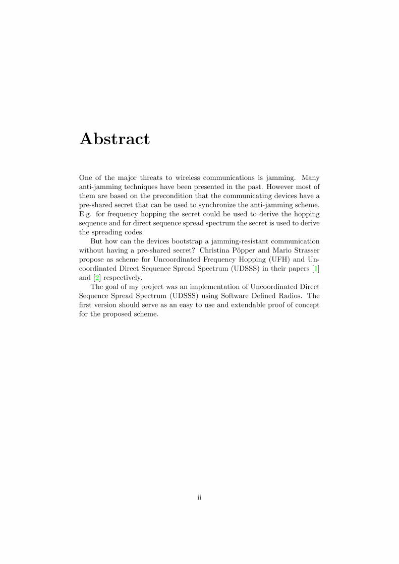
One of the major threats to wireless communications is jamming. Manyanti-jamming techniques have been presented in the past. However most ofthem are based on the precondition that the communicating devices have apre-shared secret that can be used to synchronize the anti-jamming scheme.E.g. for frequency hopping the secret could be used to derive the hoppingsequence and for direct sequence spread spectrum the secret is used to derivethe spreading codes.

But how can the devices bootstrap a jamming-resistant communicationwithout having a pre-shared secret? Christina Popper and Mario Strasserpropose as scheme for Uncoordinated Frequency Hopping (UFH) and Un-coordinated Direct Sequence Spread Spectrum (UDSSS) in their papers [1]and [2] respectively.

The goal of my project was an implementation of Uncoordinated DirectSequence Spread Spectrum (UDSSS) using Software Defined Radios. Thefirst version should serve as an easy to use and extendable proof of conceptfor the proposed scheme.

ii

Contents

Acknowledgements i

Abstract ii

1 Introduction 11.1 Jamming-resistant communication . . . . . . . . . . . . . . . 11.2 Overview . . . . . . . . . . . . . . . . . . . . . . . . . . . . . 11.3 The system . . . . . . . . . . . . . . . . . . . . . . . . . . . . 2

1.3.1 Implementation . . . . . . . . . . . . . . . . . . . . . . 21.3.2 Environment . . . . . . . . . . . . . . . . . . . . . . . 2

1.4 Chapter overview . . . . . . . . . . . . . . . . . . . . . . . . . 3

I Background 5

2 GNU Radio Overview 62.1 Introduction . . . . . . . . . . . . . . . . . . . . . . . . . . . . 62.2 A common SDR application . . . . . . . . . . . . . . . . . . . 6

2.2.1 RF front end . . . . . . . . . . . . . . . . . . . . . . . 62.2.2 The software world . . . . . . . . . . . . . . . . . . . . 92.2.3 Helpful tools . . . . . . . . . . . . . . . . . . . . . . . 9

3 DSP - As much as we need of it 103.1 Introduction . . . . . . . . . . . . . . . . . . . . . . . . . . . . 103.2 Digital filters . . . . . . . . . . . . . . . . . . . . . . . . . . . 11

3.2.1 DSP Filters in GNU Radio . . . . . . . . . . . . . . . 113.2.2 Standard filters . . . . . . . . . . . . . . . . . . . . . . 12

3.3 Translating a signal . . . . . . . . . . . . . . . . . . . . . . . 123.3.1 How does multiplication with a sine wave translate a

signal? . . . . . . . . . . . . . . . . . . . . . . . . . . . 12

iii

CONTENTS iv

II The System implementation 15

4 System Overview 164.1 The bird’s eye view . . . . . . . . . . . . . . . . . . . . . . . . 164.2 The signal pathway . . . . . . . . . . . . . . . . . . . . . . . . 17

4.2.1 Sending data . . . . . . . . . . . . . . . . . . . . . . . 174.2.2 Receiving data . . . . . . . . . . . . . . . . . . . . . . 17

5 System implementation 195.1 The sender application . . . . . . . . . . . . . . . . . . . . . . 195.2 The receiver application . . . . . . . . . . . . . . . . . . . . . 205.3 Blocks in Detail . . . . . . . . . . . . . . . . . . . . . . . . . . 20

5.3.1 Codesequence input file . . . . . . . . . . . . . . . . . 205.3.2 Class skeleton . . . . . . . . . . . . . . . . . . . . . . . 205.3.3 Sender blocks . . . . . . . . . . . . . . . . . . . . . . . 235.3.4 Receiver blocks . . . . . . . . . . . . . . . . . . . . . . 27

5.4 Summary . . . . . . . . . . . . . . . . . . . . . . . . . . . . . 31

III Experiments and Conclusions 32

6 Experiments and Measurements 336.1 Testbed layout . . . . . . . . . . . . . . . . . . . . . . . . . . 336.2 Test cases . . . . . . . . . . . . . . . . . . . . . . . . . . . . . 356.3 Results . . . . . . . . . . . . . . . . . . . . . . . . . . . . . . . 35

6.3.1 First bit times per Nr. of Codesequences . . . . . . . . 356.3.2 Message times per Nr. of Codesequences . . . . . . . . 376.3.3 Other results . . . . . . . . . . . . . . . . . . . . . . . 37

7 Conclusions 397.1 Review . . . . . . . . . . . . . . . . . . . . . . . . . . . . . . . 397.2 Lessons learned . . . . . . . . . . . . . . . . . . . . . . . . . . 39

7.2.1 Project management . . . . . . . . . . . . . . . . . . . 407.3 Future work . . . . . . . . . . . . . . . . . . . . . . . . . . . . 40

IV Appendix 42

A Project Schedule 43A.1 Review . . . . . . . . . . . . . . . . . . . . . . . . . . . . . . . 43A.2 Planned schedule . . . . . . . . . . . . . . . . . . . . . . . . . 43A.3 Actual schedule . . . . . . . . . . . . . . . . . . . . . . . . . . 43

B Preliminary presentation Jan 16, 2008 47

CONTENTS v

Bibliography 55

List of Figures

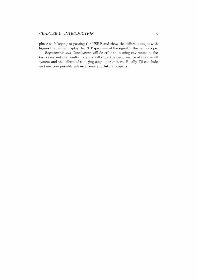
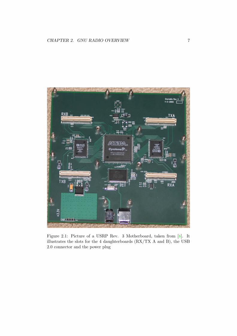
2.1 Picture of a USRP Rev. 3 Motherboard, taken from [8]. Itillustrates the slots for the 4 daughterboards (RX/TX A andB), the USB 2.0 connector and the power plug . . . . . . . . 7

2.2 Digital Down Converter Block Diagram, taken from [4]. Itconsists of a local sine/cosine generator followed by a deci-mating and low pass filter. . . . . . . . . . . . . . . . . . . . . 8

3.1 Schematic view of a DSP system [15] that starts with theanalog signal passing the ADC followed by a chain of DSPfilters and finally passing the DAC. . . . . . . . . . . . . . . . 10

3.2 A schematic view of a DSP filter that filters the raw incomingsample stream. . . . . . . . . . . . . . . . . . . . . . . . . . . 11

3.3 Multiplication of two sine waves with the same frequency f1(red and blue) results in a signal (green) containing the twofrequencies 2 · f1 and 0. . . . . . . . . . . . . . . . . . . . . . 13

3.4 FFT of the repeated data signal 00110101 before translation,i.e. in baseband . . . . . . . . . . . . . . . . . . . . . . . . . . 13

3.5 FFT of the repeated data signal 00110101 after translationby (multiplication with) a carrier at 100 kHz i.e. after car-rier modulation. The multiplication results in a shift of thebaseband signal in the frequency spectrum by 100 kHz. . . . 14

4.1 A usual SDR receiver system based on GNU Radio consistsof the USRP connected over USB to a laptop that is runningthe GNU Radio framework. . . . . . . . . . . . . . . . . . . . 16

4.2 The flowgraph of the sender application. It shows the senderblocks Sender Appl, UDSSS, PSK and USRP and the code-sequences file. . . . . . . . . . . . . . . . . . . . . . . . . . . . 17

4.3 The flowgraph of the receiver application. It shows the 4receiver blocks USRP, DePSK, DeUDSSS and Receiver Appland the file that contains the DSSS codesequences. . . . . . . 18

5.1 Codesequence file format . . . . . . . . . . . . . . . . . . . . . 21

vi

LIST OF FIGURES vii

5.2 The package format that is used by Sender Appl and ReceiverAppl to send and receive data. Each package has a staticpackage header, a unique message and package id, the payloaddata and a checksum. . . . . . . . . . . . . . . . . . . . . . . 23

5.3 The data 0110 in the time domain displayed in red. Binaryones are represented as low-values, zeros are represented ashigh-values. . . . . . . . . . . . . . . . . . . . . . . . . . . . . 24

5.4 The data 0110 displayed in red after spreading with the se-quence 0100 0101 1001 1100 (blue) results in the transmittedchip sequences (green). . . . . . . . . . . . . . . . . . . . . . . 26

5.5 The oscillograph of a modulated carrier signal with high datarate and visible phase shifts. The red and blue lines are thereal and imaginary components of the signal. . . . . . . . . . 27

5.6 The oscillograph of a distorted signal coming from the USRPwith noise, frequency offset and other attenuation. The redand blue lines are the real and imaginary components of thesignal. . . . . . . . . . . . . . . . . . . . . . . . . . . . . . . . 28

5.7 FFT of a distorted signal coming from the USRP with noise,frequency offset and other attenuation. . . . . . . . . . . . . . 28

6.1 The testbed used for the measurements. Sender and receiverare 3m apart and each connected over USB to a laptop thatis running 2 VMware machines simultaneously. . . . . . . . . 34

6.2 Comparison of first bit times against number of codesequenceswhen using 32-bit codes. Averaged over 100 measurements.The average value is represented in green, the max value inred and the min value in blue. . . . . . . . . . . . . . . . . . . 36

6.3 Comparison of first bit times against number of codesequenceswhen using 1024-bit codes. Averaged over 20 measurements.The average value is represented in green, the max value inred and the min value in blue. . . . . . . . . . . . . . . . . . . 37

6.4 Comparison of message times against number of codesequenceswhen using 32-bit codes. Averaged over 100 measurements.The average value is represented in green, the max value inred and the min value in blue. . . . . . . . . . . . . . . . . . . 38

A.1 Original project schedule including milestones. Generatedusing MindManager. . . . . . . . . . . . . . . . . . . . . . . . 45

List of Tables

A.1 Project milestones . . . . . . . . . . . . . . . . . . . . . . . . 44A.2 The actual project schedule . . . . . . . . . . . . . . . . . . . 46

viii

Listings

5.1 A headerfile template for a class extending from gr sync block.It demonstrates the minimum requirements for a DSP blockin GNU Radio . . . . . . . . . . . . . . . . . . . . . . . . . . 21

5.2 The mainloop in general work of the class tibits dsss bb. Itloops bit by bit through the input and sends the DSSS codefor a 0 or a 1 respectively to the output. . . . . . . . . . . . . 24

5.3 Function is code at from the class tibits dedsss bb. It com-pares the given chunk of input bits with the given code. . . . 30

ix

Chapter 1

Introduction

The following document is the final project report of my master thesis aboutthe implementation of a system for uncoordinated direct sequence spreadspectrum (U-DSSS).

1.1 Jamming-resistant communication

Currently one of the major threats to wireless communication is the fact thatit can easily be intercepted or jammed. Especially jamming is a topic thathas to be dealt with care because there is basically no protection against it.The attacker could potentially sit anywhere and is usually assumed to havehuge but not infinite power and processing resources.

Current known anti-jamming techniques require the communicating de-vices to have a pre-shared secret that can be used as a secret spreading key.For frequency hopping based anti-jamming schemes this key is used to de-rive the hopping sequence. For DSSS based anti-jamming schemes the keyis used to derive the codesequences.

1.2 Overview

My work is based on the papers [1] and [2] published by my supervisorsChristina Popper and Mario Strasser. In order to be able to fully appreciateand see behind the scenes of the implementation the reader might need toread these papers first.

The papers aim at finding an answer to the following question: “howcan two devices that do not share any secrets establish a shared secretkey over a wireless radio channel in the presence of a communication jam-mer?”. In the assumptions of this question no pre-shared secret exists socurrent anti-jamming techniques fail to accomplish this task. The proposedU-DSSS scheme however solves this issue in the following way: The jamming-resistance property of the channel is achieved as usual by choosing secret

1

CHAPTER 1. INTRODUCTION 2

DSSS codesequences. However since the two devices don’t share any secretsthat could be used to agree on a sequence, the sequences are chosen ran-domly from a given range. Although this channel is very error-prone and nofast or completely reliable communication is possible, the properties sufficeto perform a key establishment protocol that will result in a key which thencan be used to agree on a secret DSSS codesequence.

1.3 The system

1.3.1 Implementation

The system described in this document is a proof of concept for the pro-posed scheme. The declared aim was clearly an easy to use implementationthat serves as a proof of concept, can easily be extended and is able to pro-duce well-traceable results for further research. Performance and robustnessissues were also taken into account but had a lower priority.

The main project delivery consisted of the system itself as a VMware im-age, including the full sourcecode, a detailed class documentation generatedwith Doxygen, short preliminary project reports and presentations, this finalreport, the measured results, many C++ and Python examples and manytest files which were extensively used during the development phase.

Throughout this report I’ll try to explain or at least provide links toeverything the reader needs to know in order to be able to completely followthe implementation of the system. My aim is that, following this reportand the provided links, the reader should actually be able to implement thesystem on his own or implement similar systems without having to wastetoo much time on gathering the necessary background information.

1.3.2 Environment

For the implementation I used software-defined radios (SDR), where theGNU Radio framework [3] probably is the current state-of-the-art. SDRsallow the developer to implement the whole signal processing blocks com-pletely in software, giving him the freedom to code exactly the propertiesthat are needed for the system. As RF front ends I used 2 USRPs [8]equipped with the RFX2400 daughterboards, having the following charac-teristics [9]:

• Frequency range between 2.3 GHz - 2.9 GHz

• Four 64 MS/s 12-bit analog to digital Converters

• Four 128 MS/s 14-bit digital to analog Converters

• Four digital downconverters with programmable decimation rates

CHAPTER 1. INTRODUCTION 3

• Two digital upconverters with programmable interpolation rates

• High-speed USB 2.0 interface (480 Mb/s)

DSP blocks

Although GNU Radio provides a big set of standard DSP (digital signalprocessing) blocks the overlap with what I needed was so small that I decidedto implement the whole system from scratch without reusing the existingcode. That way I was able to get rid of overhead like error correction or theGNU Radio way of packaging data into message blocks, which would havehad an impact on the system performance and thus dilute the measuredperformance times. Also that way when running into problems I was quicklyable to tweak exactly these parts of the system that needed to be changed.

Deployment details

All the coding and the tests were done inside a VMware Player [11] (Version2.0.1 build-55017) running an Ubuntu 7.10 Gutsy Gibbon [12] guest OS anda manually installed GNU Radio 3.1.1 release. This way the deployment canbe done very easily by burning the VMware image on a DVD which will runon any host OS that is supported by the VMware Player. The developmentinstallation ran on an IBM ThinkPad Lenovo T61.

1.4 Chapter overview

This report is split into 4 Parts: Background, The System implementation,Experiments and Conclusions and finally the Appendix. Throughout thewhole report I’ve set great value on providing the reader with useful linksand resources that I’ve found during the work on my project.

In the background part I’ll try to cover and summarize all the importantknowledge that I’ve learned during my work. There will be a chapter aboutDSP and one about SDRs and GNU Radio [3] in general. However sincethere are already very good resources available about DSP and GNU Radioand a detailed description would be outside the scope of this report, I’ll justsummarize the most important facts needed for this report and guide thereader to online resources for further information. Thus in the bibliographyat the end of this report there will be a great collection of links about allthe covered topics.

The part about the system implementation will cover the actual work I’vedone during the last few months. It’ll contain an overview of the system onthe whole and then go into the details of the individual blocks. I’ll alsoexplain the signal path of a datablock from DSSS spreading over binary

CHAPTER 1. INTRODUCTION 4

phase shift keying to passing the USRP and show the different stages withfigures that either display the FFT spectrum of the signal or the oscilloscope.

Experiments and Conclusions will describe the testing environment, thetest cases and the results. Graphs will show the performance of the overallsystem and the effects of changing single parameters. Finally I’ll concludeand mention possible enhancements and future projects.

Part I

Background

5

Chapter 2

GNU Radio Overview

2.1 Introduction

GNU Radio provides an open source framework for developing SDRs. Dueto it’s flexibility and motivated community it represents the current state-of-the-art for SDRs. Also the GNU Radio Development Team developed abig set of filters and applications that can easily be extended and adaptedto the current needs.

To support the further development and to add a flexible open source RFfront end to GNU Radio, Matt Ettus, a member of the GNU Radio Team,founded the Ettus Research LLC [8] and started to build the Universal Soft-ware Radio Peripheral (USRP). This device is built using a flexible, opensource design that allows 4 different daugherboards to be connected to it,each daughterboard working on its own frequency range. Currently daugh-terboards are available for the ranges between DC up to 2.9 GHz. Probablythe most used daughterboard is the RFX2400 which is a transceiver between2.3 GHz to 2.9 GHz.

Figure 2.1 shows the USRP Motherboard.

2.2 A common SDR application

The information summarized in this chapter was found at [3], [4], [5], [6]and [7] which together represent a great resource for starting with SDR andGNU Radio.

2.2.1 RF front end

A common SDR system consists of the RF frond end that is connected toan ADC (analog to digital converter) which produces more or less highspeeddata samples. These samples are completely processed in software, the ap-plication code and the DSP filters. For a GNU Radio application the RF

6

CHAPTER 2. GNU RADIO OVERVIEW 7

Figure 2.1: Picture of a USRP Rev. 3 Motherboard, taken from [8]. Itillustrates the slots for the 4 daughterboards (RX/TX A and B), the USB2.0 connector and the power plug

CHAPTER 2. GNU RADIO OVERVIEW 8

front end and the DAC/ADC is implemented in the USRP. It can be seen asa blackbox that has just 1 input which is the RX/TX center frequency. Alldata, that is sent to the USRP is modulated to (multiplied by) the carrierfrequency which results in a translation of the baseband signal to the carrierfrequency in the analog domain. However for USRPs this translation is notdone directly but it’s split into 2 distinct parts: the analog and the digitalpart.

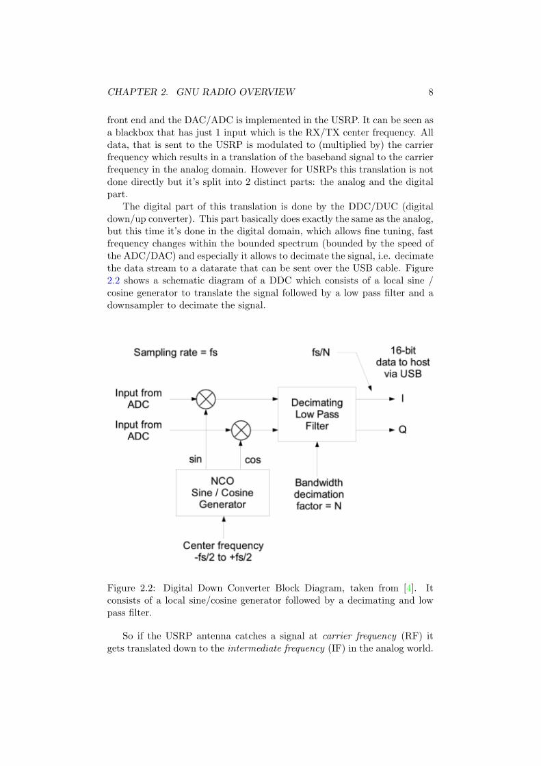
The digital part of this translation is done by the DDC/DUC (digitaldown/up converter). This part basically does exactly the same as the analog,but this time it’s done in the digital domain, which allows fine tuning, fastfrequency changes within the bounded spectrum (bounded by the speed ofthe ADC/DAC) and especially it allows to decimate the signal, i.e. decimatethe data stream to a datarate that can be sent over the USB cable. Figure2.2 shows a schematic diagram of a DDC which consists of a local sine /cosine generator to translate the signal followed by a low pass filter and adownsampler to decimate the signal.

Figure 2.2: Digital Down Converter Block Diagram, taken from [4]. Itconsists of a local sine/cosine generator followed by a decimating and lowpass filter.

So if the USRP antenna catches a signal at carrier frequency (RF) itgets translated down to the intermediate frequency (IF) in the analog world.

CHAPTER 2. GNU RADIO OVERVIEW 9

That’s where the ADC digitizes the signal and forwards the samples to theDDC. The DDC decimates the signal, applies a lowpass filter and translatesit down to baseband before sending it over USB to the software world.

2.2.2 The software world

Now the GNU Radio framework takes care of the software world, i.e. itprovides interfaces to the USRP, cares about data buffering and linking thecustom DSP filters together.

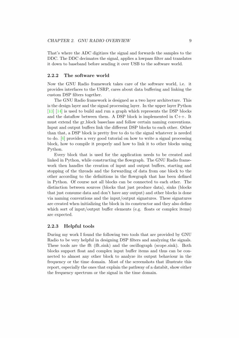
The GNU Radio framework is designed as a two layer architecture. Thisis the design layer and the signal processing layer. In the upper layer Python[13] [14] is used to build and run a graph which represents the DSP blocksand the dataflow between them. A DSP block is implemented in C++. Itmust extend the gr block baseclass and follow certain naming conventions.Input and output buffers link the different DSP blocks to each other. Otherthan that, a DSP block is pretty free to do to the signal whatever is neededto do. [6] provides a very good tutorial on how to write a signal processingblock, how to compile it properly and how to link it to other blocks usingPython.

Every block that is used for the application needs to be created andlinked in Python, while constructing the flowgraph. The GNU Radio frame-work then handles the creation of input and output buffers, starting andstopping of the threads and the forwarding of data from one block to theother according to the definitions in the flowgraph that has been definedin Python. Of course not all blocks can be connected to each other. Thedistinction between sources (blocks that just produce data), sinks (blocksthat just consume data and don’t have any output) and other blocks is donevia naming conventions and the input/output signatures. These signaturesare created when initializing the block in its constructor and they also definewhich sort of input/output buffer elements (e.g. floats or complex items)are expected.

2.2.3 Helpful tools

During my work I found the following two tools that are provided by GNURadio to be very helpful in designing DSP filters and analyzing the signals.These tools are the fft (fft sink) and the oscillograph (scope sink). Bothblocks support float and complex input buffer items and thus can be con-nected to almost any other block to analyze its output behaviour in thefrequency or the time domain. Most of the screenshots that illustrate thisreport, especially the ones that explain the pathway of a databit, show eitherthe frequency spectrum or the signal in the time domain.

Chapter 3

DSP - As much as we needof it

3.1 Introduction

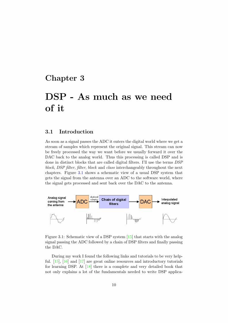
As soon as a signal passes the ADC it enters the digital world where we get astream of samples which represent the original signal. This stream can nowbe freely processed the way we want before we usually forward it over theDAC back to the analog world. Thus this processing is called DSP and isdone in distinct blocks that are called digital filters. I’ll use the terms DSPblock, DSP filter, filter, block and class interchangeably throughout the nextchapters. Figure 3.1 shows a schematic view of a usual DSP system thatgets the signal from the antenna over an ADC to the software world, wherethe signal gets processed and sent back over the DAC to the antenna.

Figure 3.1: Schematic view of a DSP system [15] that starts with the analogsignal passing the ADC followed by a chain of DSP filters and finally passingthe DAC.

During my work I found the following links and tutorials to be very help-ful. [15], [16] and [17] are great online resources and introductory tutorialsfor learning DSP. At [18] there is a complete and very detailed book thatnot only explains a lot of the fundamentals needed to write DSP applica-

10

CHAPTER 3. DSP - AS MUCH AS WE NEED OF IT 11

tions but also demostrates the knowledge with many examples and goes intodeep details on signal analysis. Also an excellent book on DSP systems andDigital communication is [19] by John G. Proakis.

3.2 Digital filters

The function of a filter in general is, as the name suggests, to filter a sig-nal. This filtering can be anything from smoothing the signal, removingunwanted frequencies or noise or evaluating a certain function over the sig-nal on the whole. Thus a filter is usually defined over its input/outputbehaviour. A digital filter processes the signal in the digital domain, work-ing on the discretized sample stream. Figure 3.2 shows a schematic view ofa filter.

Figure 3.2: A schematic view of a DSP filter that filters the raw incomingsample stream.

With the evolution of todays CPU processing speeds almost every func-tion can be implemented as a digital filter without the need of using itsanalog counterpart.

3.2.1 DSP Filters in GNU Radio

As mentioned in the chapter about GNU Radio, the framework providesan easy, buffer-based interface to write own DSP filters and to link themtogether by defining the flowgraph in Python. GNU Radio connects thefilters by adding input and output buffers to them. These buffers can containany standard basetype available in C++ like complex, floats or integers. Inorder to connect one filter to another the items of the first filters outputbuffer are then forwarded to the input buffer of the second filter.

The developer is free to choose one of the many standard filters or maywrite his own one. When following some naming conventions and guidelines,defined in [5], writing an own filter consist mostly of only implementing themain processing function called work. This function gets the input andoutput buffers as parameters and is free to perform any functions on thisdata.

CHAPTER 3. DSP - AS MUCH AS WE NEED OF IT 12

3.2.2 Standard filters

The GNU Radio framework provides a very easy way to define a set ofstandard filters. Among these filters there are also the well-known standardones like low pass, high pass, band pass or band reject. What makes thesefilters so valuable is the fact that their behaviour can be easily changedin software while the system is initialized. Also their inherent propertieslike cut-off frequency, gain, transition width, . . . can freely be defined atstartup.

3.3 Translating a signal

DSP filters usually work with the raw signal at baseband. However a sig-nal when it’s transmitted over the antenna is usually not transmitted atbaseband because that way different applications would collide with eachother and the usable spectrum would be very limited. To solve these issuesthe data signal is used to modulate a much higher frequency signal: thecarrier signal. This action will translate the data signal from baseband toa frequency band around the carrier frequency. As already mentioned inthe GNU Radio chapter, for our application this translation is done in theUSRP and the DDC/DUC. Figure 2.2 showed the schema of a DDC thatmultiplies the data signal with a locally generated sine / cosine wave in orderto translate it from the intermediate frequency (IF) to baseband.

3.3.1 How does multiplication with a sine wave translate asignal?

Multiplication of 2 signals with frequencies f1 and f2 will result in a signalthat contains the frequencies f1 + f2 and f1 − f2. Applying a low passfilter will get rid of the signal at f1 + f2 leaving just the f1− f2 signal asa result. That’s exactly what happens when the DDC translates a signalfrom IF to baseband.

If one of the 2 original signals is just a single sine wave, i.e. a single-frequency signal (f1), then the above equations imply that all frequenciesof the other signal get translated by f1. Figure 3.3 displays this. It showsthe result of a multiplication of 2 sine waves (red and blue) with the samefrequency. This multiplication results in a new sine wave (green) with fre-quency 2 ∗ f1, because the other part of the resulting signal f1 − f2 iszero.

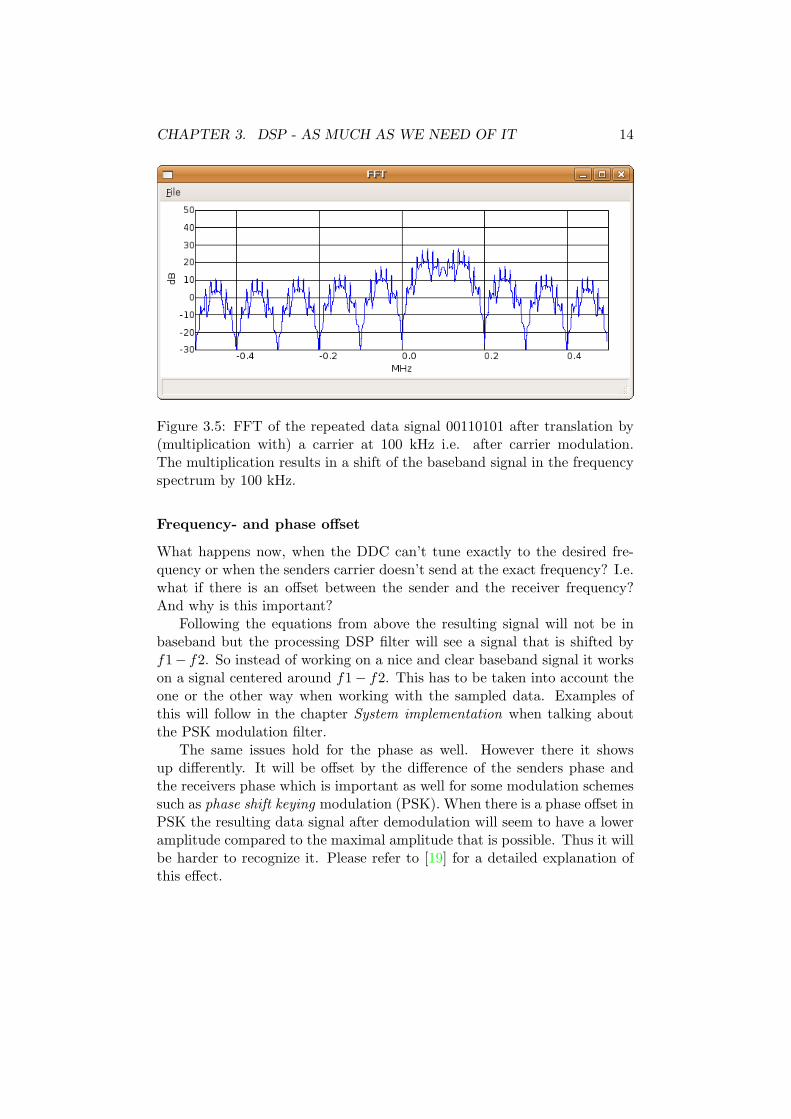
Figures 3.4 and 3.5 show the FFT of a data signal that consists of the fol-lowing sequence 00110101. The figures show the data signal before and aftermultiplication with a sine wave at 100 kHz, i.e. before and after translation.

CHAPTER 3. DSP - AS MUCH AS WE NEED OF IT 13

Figure 3.3: Multiplication of two sine waves with the same frequency f1 (redand blue) results in a signal (green) containing the two frequencies 2 · f1and 0.

Figure 3.4: FFT of the repeated data signal 00110101 before translation,i.e. in baseband

CHAPTER 3. DSP - AS MUCH AS WE NEED OF IT 14

Figure 3.5: FFT of the repeated data signal 00110101 after translation by(multiplication with) a carrier at 100 kHz i.e. after carrier modulation.The multiplication results in a shift of the baseband signal in the frequencyspectrum by 100 kHz.

Frequency- and phase offset

What happens now, when the DDC can’t tune exactly to the desired fre-quency or when the senders carrier doesn’t send at the exact frequency? I.e.what if there is an offset between the sender and the receiver frequency?And why is this important?

Following the equations from above the resulting signal will not be inbaseband but the processing DSP filter will see a signal that is shifted byf1− f2. So instead of working on a nice and clear baseband signal it workson a signal centered around f1− f2. This has to be taken into account theone or the other way when working with the sampled data. Examples ofthis will follow in the chapter System implementation when talking aboutthe PSK modulation filter.

The same issues hold for the phase as well. However there it showsup differently. It will be offset by the difference of the senders phase andthe receivers phase which is important as well for some modulation schemessuch as phase shift keying modulation (PSK). When there is a phase offset inPSK the resulting data signal after demodulation will seem to have a loweramplitude compared to the maximal amplitude that is possible. Thus it willbe harder to recognize it. Please refer to [19] for a detailed explanation ofthis effect.

Part II

The System implementation

15

Chapter 4

System Overview

4.1 The bird’s eye view

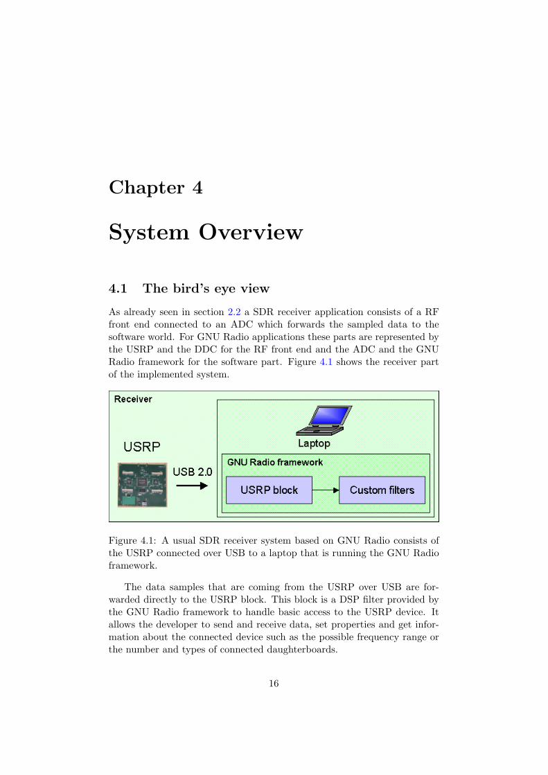
As already seen in section 2.2 a SDR receiver application consists of a RFfront end connected to an ADC which forwards the sampled data to thesoftware world. For GNU Radio applications these parts are represented bythe USRP and the DDC for the RF front end and the ADC and the GNURadio framework for the software part. Figure 4.1 shows the receiver partof the implemented system.

Figure 4.1: A usual SDR receiver system based on GNU Radio consists ofthe USRP connected over USB to a laptop that is running the GNU Radioframework.

The data samples that are coming from the USRP over USB are for-warded directly to the USRP block. This block is a DSP filter provided bythe GNU Radio framework to handle basic access to the USRP device. Itallows the developer to send and receive data, set properties and get infor-mation about the connected device such as the possible frequency range orthe number and types of connected daughterboards.

16

CHAPTER 4. SYSTEM OVERVIEW 17

In my system I used 2 USRPs for the sender and the receiver. Each ofthem is connected to a separate VMware machine running on the laptop. Asdaughterboards I used the RFX2400 devices which transmit in the frequencyrange of 2.3 GHz - 2.9GHz.

4.2 The signal pathway

Once the block diagram is clear, connecting the blocks in Python is verystraightforward. That’s why I’m not going to explain the Python world anyfurther but instead show figures of the corresponding flowgraphs.

4.2.1 Sending data

The sending application starts with the Sender block. This block generatesrandom test data and packs it into packages that are recognizable by thereceiver. These packages contain the message id, the payload data and thecrc which is used by the receiver to verify the correct transmission of thedata. I’ll show the exact package format in figure 5.2.

Such a packet is forwarded to the DSSS block. There each databitgets spread using the corresponding code from the randomly chosen code-sequence. For each packet a random codesequence is chosen and the wholemessage is spread with this sequence. The codesequences are chosen from alist in a codefile as shown in figure 4.2. A definition of the codefile formatwill follow in the next chapter.

Now the spread signal is forwarded to the PSK block for modulationand finally it’s sent over the USRP block to the air. The sender flowgraphis shown in figure 4.2.

Figure 4.2: The flowgraph of the sender application. It shows the senderblocks Sender Appl, UDSSS, PSK and USRP and the codesequences file.

4.2.2 Receiving data

The receiving application is the counterpart to the sender. After passingthe USRP block the data enters my code where the whole processing starts.I chose differential binary phase shift keying (DBPSK) modulation for thesystem due to its simplicity and straightforward implementation. BPSK

CHAPTER 4. SYSTEM OVERVIEW 18

modulates the signal by changing the carriers phase. Binary implies thatthere are only 2 distinct phases, 1 and −1.

So the first block after the USRP block is called DePSK. It demodu-lates the incoming BPSK signal and performs chip synchronization. Sincefor the test layout and results it didn’t matter if the signal was weaker orstronger than the noiselevel I could make it so strong that it could easilybe distinguished from the noise. That way the chip synchronization couldbe based on analyzing the incoming signal directly without having to de-spread the signal first. This of course has a big impact on the overall systemperformance as we will see when talking about the test results.

After demodulating the signal it needs to get despread. This is donein the DeDSSS block which of course needs to find the correct DSSS codesequence first before it despreads the signal. The crucial part here is thenumber of possible codesequences that need to be searched in order to findthe right code. This value also directly impacts the overall performance ofthe system. However since the chip synchronization is already done at thispoint, the time to find the right codesequence is linear in the number ofsequences.

Finally the Receiver block receives the data, performs a checksum veri-fication to check if the data is valid and was correctly transmitted. It alsohandles the time measurement for the test cases if the data verification wassuccessful.

The flowgraph that needs to be defined in Python is shown in figure 4.3.It represents the DSP blocks as rectangles and the linkage between themwith arrows.

Figure 4.3: The flowgraph of the receiver application. It shows the 4 re-ceiver blocks USRP, DePSK, DeUDSSS and Receiver Appl and the file thatcontains the DSSS codesequences.

Chapter 5

System implementation

The last chapters provided a good overview of what the final system lookslike. In the introductory chapters GNU Radio and DSP we saw how theGNU Radio framework can help to implement a SDR application. Also wesaw an overview on how DSP filters can be implemented and how they canbe linked together to a complete application. System design decisions wereexplained in the last chapter which together formed the foundation for thedetailed system design explained in this chapter.

This chapter follows the signal pathway from the sender application tothe receiver and will explain every block on this path in detail. Where ithelps the understanding I’ll add snippets of the sourcecode or of the detailedclass documentation that was generated with Doxygen [20]. Every blockdocumentation is arranged the following way: It starts with a block overviewthat explains the processing result from a signal and design perspective andthe input/output behaviour. Then a detailed class description will followthat includes the most important functions and their interface, if it supportsthe understanding. Finally I’ll conclude the description by displaying howthe signal changes either in the frequency or in the time domain which isprobably the most interesting part from a DSP point of view.

5.1 The sender application

As has been seen in the system overview both the sender and the receiverapplications run inside separate VMware machines. However all blocks areinstalled on both machines. Actually the development is done on one ma-chine which is then copied and renamed to a different directory on the hostmachine before starting a second VMware Player and running the tests.

The sender application consist of the Sender Appl, UDSSS and the PSKblocks and the Python file that creates them and links them together. Figure4.2 shows the corresponding flowgraph. These blocks together generate thetest data and send it over the USRP to the receiver application. Time mea-

19

CHAPTER 5. SYSTEM IMPLEMENTATION 20

surement which is needed for the tests is done by using timestamps. Sinceboth VMware machines run on the same host environment the time mea-surement could easily be done by comparing timestamps directly withouthaving to synchronize the two applications first.

5.2 The receiver application

A schematic overview of the receiver application has been shown in figure4.3. It consist of the blocks DePSK, DeUDSSS and Receiver Appl whichtogether decode the test data, perform checksum verification and store themeasured times for the statistics. This processing can either be done onlineor offline. When the processing is done offline then the Python file replacesthe USRP block by a Filesource and connects it to the DePSK.

5.3 Blocks in Detail

5.3.1 Codesequence input file

When looking at the sender and receiver flowgraphs one can see anotherblock called codes. This block is not a DSP filter but a file that is used bythe two DSSS classes. This file defines the different codesequences that canbe used by the DSSS classes. Both classes read the file at startup and cacheall the defined sequences in a local variable for later use.

Now what is a codesequence?

As usual for DSSS each input bit is spread by a code. For U-DSSS the choiceof the current code is random. But instead of using a random code froma list the U-DSSS chooses a random codesequence where the codesequencedefines exactly which bit of the input message is spread by which code.This means for example that for a message with a length of 1024 bits thecodesequence must contain 1024 codes.

File format

A codesequence file defines the number of codesequences(k), the bitlengthof a message(n), the chiplength of a code(N) and finally the codesequencesthemselves. The single chips are written by ‘+’/‘1’ or ‘-’/‘0’. A chip isrepresented as < cknN > in the file format specification that is shown infigure 5.1.

5.3.2 Class skeleton

Of course a block that wants to be supported by the GNU Radio frameworkneeds to implement certain functions and fulfil certain criteria. Please refer

CHAPTER 5. SYSTEM IMPLEMENTATION 21

Figure 5.1: Codesequence file format

<nr. of codesequences(k)> <message bitlen(n)> <code bitlen(N)><c111><c112>...<c11N><c121><c122>...<c12N>...<c1n1><c1n2>...<c1nN><c211><c212>...<c21N><c221><c222>...<c22N>...<c2n1><c2n2>...<c2nN>...... ...<ck11><ck12>...<ck1N><ck21><ck22>...<ck2N>...<ckn1><ckn2>...<cknN>

to [6] for a complete listing of these criteria.To ease the development the framework provides a number of base classes

that can easily be extended to implement the desired DSP functionality. Themost commonly used base classes are gr block and gr sync block where themain difference between them is that gr sync block assumes that there arealways as many output items as there are input items.

When extending from gr sync block all that at least needs to be im-plemented is the function work which directly handles the data processing.When extending from gr block there are the functions general work andforecast which need to be implemented where general work has basicallythe same scope as work and forecast is needed to forecast the number ofinput items needed when the number of output items is given.

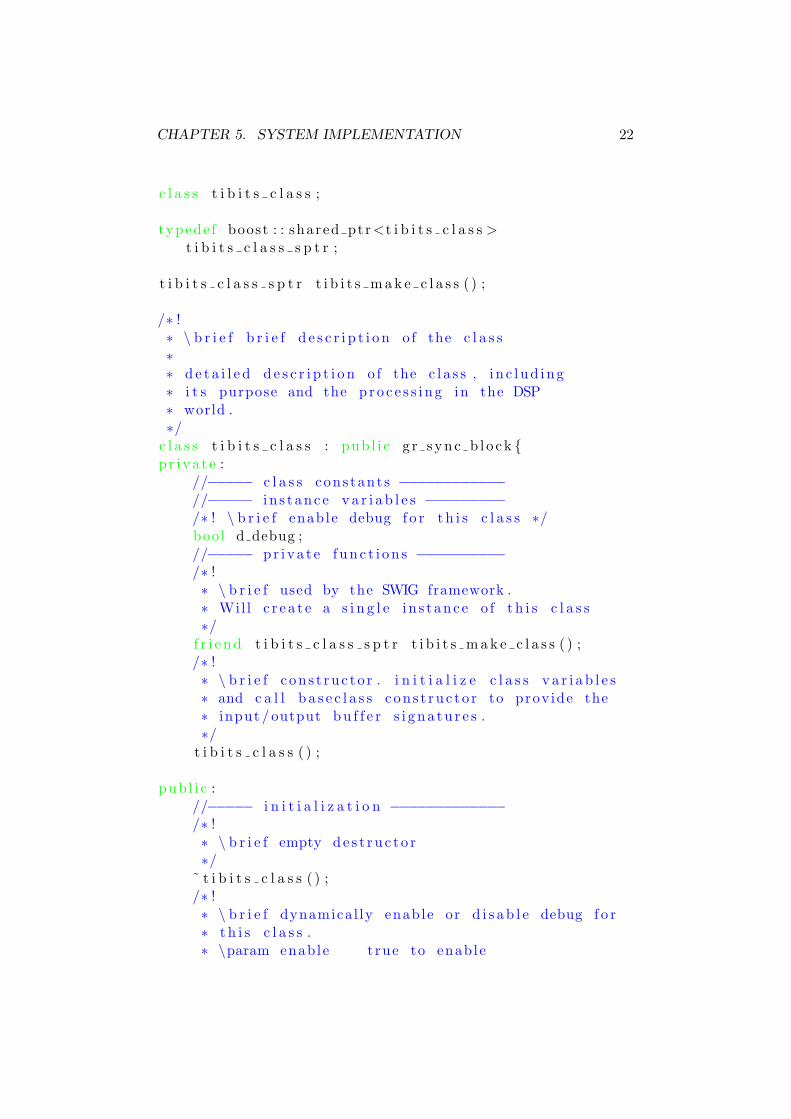
What follows is a listing of a headerfile template that I used during mydevelopment phase. The listing should demonstrate the reader how smalla minimal DSP class could be while still obeying the guidelines for a blockusable by the framework. Comments that start with ! contain tags, e.g.brief used by Doxygen to produce a javadoc-like documentation in html.

Listing 5.1: A headerfile template for a class extending from gr sync block.It demonstrates the minimum requirements for a DSP block in GNU Radio

#i f n d e f TIBITS CLASS#d e f i n e TIBITS CLASS

#inc lude <g r s y n c b l o c k . h>

CHAPTER 5. SYSTEM IMPLEMENTATION 22

c l a s s t i b i t s c l a s s ;

typede f boost : : shared ptr<t i b i t s c l a s s >t i b i t s c l a s s s p t r ;

t i b i t s c l a s s s p t r t i b i t s m a k e c l a s s ( ) ;

/∗ !∗ \ b r i e f b r i e f d e s c r i p t i o n o f the c l a s s∗∗ d e t a i l e d d e s c r i p t i o n o f the c l a s s , i n c l u d i n g∗ i t s purpose and the p r o c e s s i n g in the DSP∗ world .∗/

c l a s s t i b i t s c l a s s : pub l i c g r s y n c b l o c k {p r i v a t e :

//−−−−− c l a s s cons tant s −−−−−−−−−−−−//−−−−− i n s t anc e v a r i a b l e s −−−−−−−−−/∗ ! \ b r i e f enable debug f o r t h i s c l a s s ∗/bool d debug ;//−−−−− p r i v a t e f u n c t i o n s −−−−−−−−−−/∗ !∗ \ b r i e f used by the SWIG framework .∗ Will c r e a t e a s i n g l e i n s t anc e o f t h i s c l a s s∗/

f r i e n d t i b i t s c l a s s s p t r t i b i t s m a k e c l a s s ( ) ;/∗ !∗ \ b r i e f c on s t ruc to r . i n i t i a l i z e c l a s s v a r i a b l e s∗ and c a l l b a s e c l a s s con s t ruc to r to prov ide the∗ input / output b u f f e r s i g n a t u r e s .∗/

t i b i t s c l a s s ( ) ;

pub l i c ://−−−−− i n i t i a l i z a t i o n −−−−−−−−−−−−−/∗ !∗ \ b r i e f empty d e s t r u c t o r∗/

˜ t i b i t s c l a s s ( ) ;/∗ !∗ \ b r i e f dynamical ly enable or d i s a b l e debug f o r∗ t h i s c l a s s .∗ \param enable t rue to enable

CHAPTER 5. SYSTEM IMPLEMENTATION 23

∗/void enable debug ( i n t enable ) { d debug = enable ;}

//−−−−− o v e r r i d e s g r s y n c b l o c k −−−−/∗ !∗ \ b r i e f main p r o c e s s i n g func t i on∗∗ Cal led by the framework to perform the∗ p r o c e s s i n g .∗ \param noutput i tems number o f output items∗ \param input i t ems ptr to the input b u f f e r∗ \param output i tems ptr to the input b u f f e r∗ \ r e tu rn s the number o f produced output e lements∗/

i n t work ( i n t noutput items ,g r v e c t o r c o n s t v o i d s t a r &input i tems ,g r v e c t o r v o i d s t a r &output i tems ) ;

} ;#e n d i f

5.3.3 Sender blocks

The overview of the sender blocks was shown in figure 4.2. Here is the classdescription of the three classes.

Sender Appl

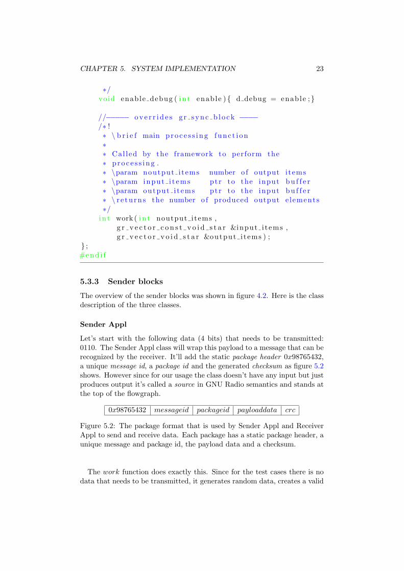
Let’s start with the following data (4 bits) that needs to be transmitted:0110. The Sender Appl class will wrap this payload to a message that can berecognized by the receiver. It’ll add the static package header 0x98765432,a unique message id, a package id and the generated checksum as figure 5.2shows. However since for our usage the class doesn’t have any input but justproduces output it’s called a source in GNU Radio semantics and stands atthe top of the flowgraph.

0x98765432 messageid packageid payloaddata crc

Figure 5.2: The package format that is used by Sender Appl and ReceiverAppl to send and receive data. Each package has a static package header, aunique message and package id, the payload data and a checksum.

The work function does exactly this. Since for the test cases there is nodata that needs to be transmitted, it generates random data, creates a valid

CHAPTER 5. SYSTEM IMPLEMENTATION 24

message in the above format and sends it to the output buffer using thenative C memcpy function.

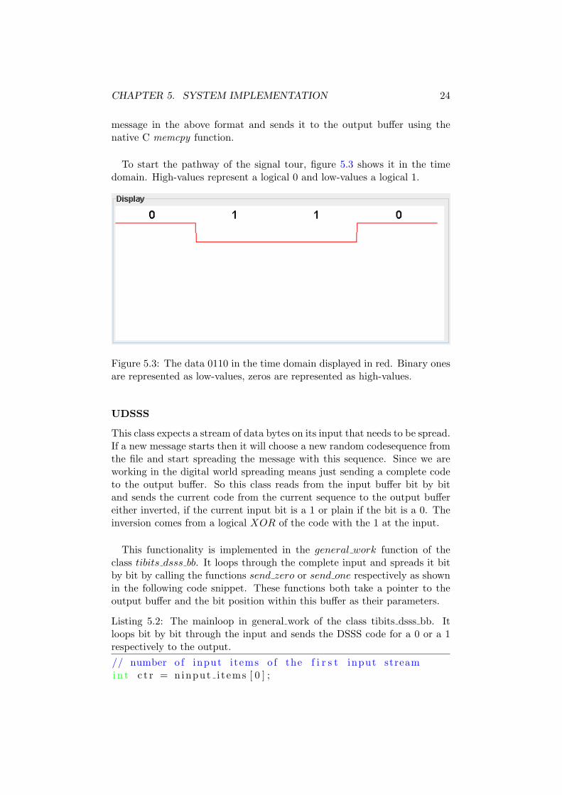
To start the pathway of the signal tour, figure 5.3 shows it in the timedomain. High-values represent a logical 0 and low-values a logical 1.

Figure 5.3: The data 0110 in the time domain displayed in red. Binary onesare represented as low-values, zeros are represented as high-values.

UDSSS

This class expects a stream of data bytes on its input that needs to be spread.If a new message starts then it will choose a new random codesequence fromthe file and start spreading the message with this sequence. Since we areworking in the digital world spreading means just sending a complete codeto the output buffer. So this class reads from the input buffer bit by bitand sends the current code from the current sequence to the output buffereither inverted, if the current input bit is a 1 or plain if the bit is a 0. Theinversion comes from a logical XOR of the code with the 1 at the input.

This functionality is implemented in the general work function of theclass tibits dsss bb. It loops through the complete input and spreads it bitby bit by calling the functions send zero or send one respectively as shownin the following code snippet. These functions both take a pointer to theoutput buffer and the bit position within this buffer as their parameters.

Listing 5.2: The mainloop in general work of the class tibits dsss bb. Itloops bit by bit through the input and sends the DSSS code for a 0 or a 1respectively to the output.// number o f input items o f the f i r s t input streami n t c t r = ninput i t ems [ 0 ] ;

CHAPTER 5. SYSTEM IMPLEMENTATION 25

f o r ( i =0; i<c t r ; i++){// range check . we need at l e a s t 1 f u l l bytei f ( ( b i t c t r >> 3) > ( noutput items −2) ) break ;// e x t r a c t s i n g l e b i t s from current databytebyte andmask = 0x80 ;// spread 1 bytef o r ( i n t j =0; j <8; j++){

i f ( ( input [ i ] & andmask ) == 0)b i t c t r += send ze ro ( output , b i t c t r ) ;

e l s eb i t c t r += send one ( output , b i t c t r ) ;

andmask >>= 1 ;// next code from current sequenced curch ipseq++;

}// i f cur rent message i s f u l l y spreadi f ( d curch ipseq >= d msgbi t l en ) {

// message f i n i s h e d −> choose new sequenced curch ipseq = 0 ;d curcodeseq = rand ( ) % d ncodes ;

}}

However a GNU Radio application is purely stream-based and thereis no direct communication between the different classes. There is justdata buffers that connect them. So e.g. there is no possibility to ‘tell’the next block that a new message has started. Strictly speaking the func-tion general work gets a chunk of data in the input buffer, whatever thisdata is. That’s why there is no concrete notion of a message in this class.

Since GNU Radio handles the buffering, the original message could besplit into multiple parts and subsequent calls to general work would eachget one of these parts. Or it’s also possible that there could be multiplemessages within the same buffer which is passed to the function in onesingle call.

Thus the decision on when to start a new codesequence is based on thenumber of bits that were already spread. So it starts spreading with a newcodesequence after every n-th bit.

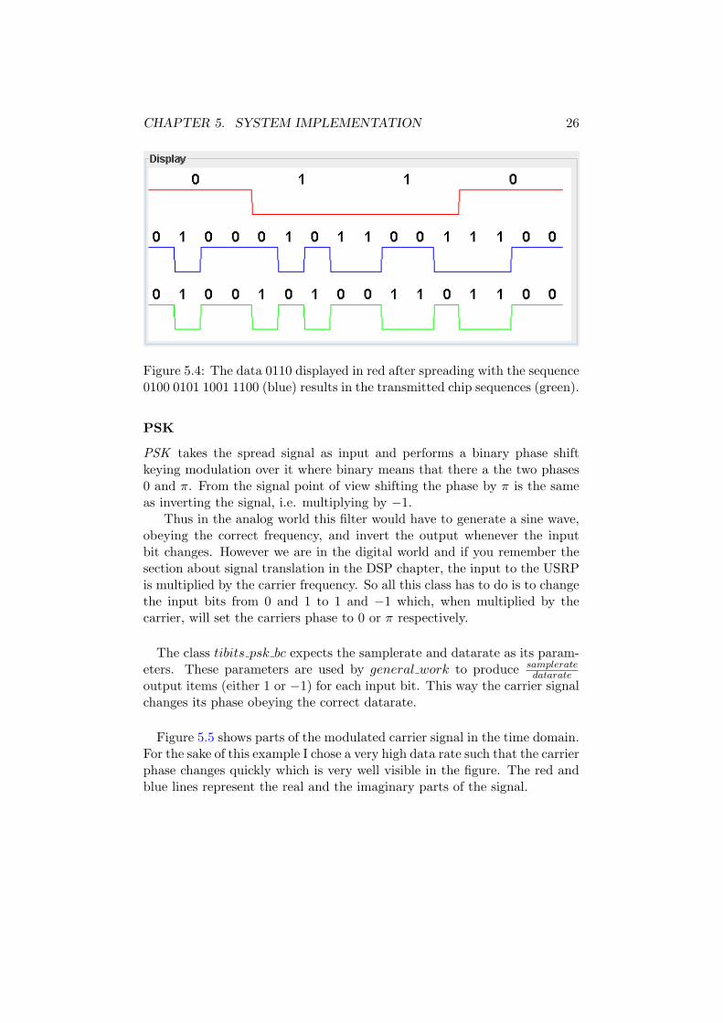
Following the pathway to the next block, the data bits 0110 are nowspread with a random codesequence. Assuming the chosen codesequencewith k = 1, n = 4, N = 4 was 0100 0101 1001 1100 then the signal wouldlook as figure 5.4 shows. The red signal is the original data, the blue one isthe spreading code and green is the resulting signal.

CHAPTER 5. SYSTEM IMPLEMENTATION 26

Figure 5.4: The data 0110 displayed in red after spreading with the sequence0100 0101 1001 1100 (blue) results in the transmitted chip sequences (green).

PSK

PSK takes the spread signal as input and performs a binary phase shiftkeying modulation over it where binary means that there a the two phases0 and π. From the signal point of view shifting the phase by π is the sameas inverting the signal, i.e. multiplying by −1.

Thus in the analog world this filter would have to generate a sine wave,obeying the correct frequency, and invert the output whenever the inputbit changes. However we are in the digital world and if you remember thesection about signal translation in the DSP chapter, the input to the USRPis multiplied by the carrier frequency. So all this class has to do is to changethe input bits from 0 and 1 to 1 and −1 which, when multiplied by thecarrier, will set the carriers phase to 0 or π respectively.

The class tibits psk bc expects the samplerate and datarate as its param-eters. These parameters are used by general work to produce samplerate

datarateoutput items (either 1 or −1) for each input bit. This way the carrier signalchanges its phase obeying the correct datarate.

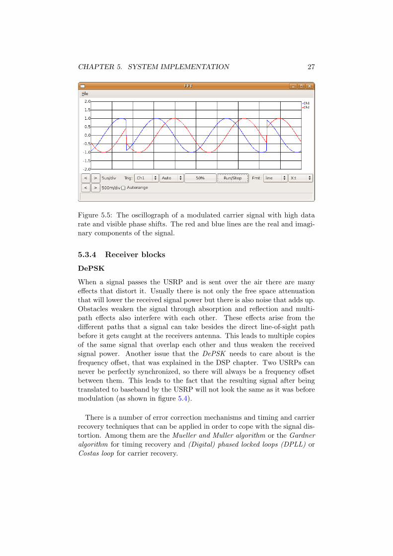
Figure 5.5 shows parts of the modulated carrier signal in the time domain.For the sake of this example I chose a very high data rate such that the carrierphase changes quickly which is very well visible in the figure. The red andblue lines represent the real and the imaginary parts of the signal.

CHAPTER 5. SYSTEM IMPLEMENTATION 27

Figure 5.5: The oscillograph of a modulated carrier signal with high datarate and visible phase shifts. The red and blue lines are the real and imagi-nary components of the signal.

5.3.4 Receiver blocks

DePSK

When a signal passes the USRP and is sent over the air there are manyeffects that distort it. Usually there is not only the free space attenuationthat will lower the received signal power but there is also noise that adds up.Obstacles weaken the signal through absorption and reflection and multi-path effects also interfere with each other. These effects arise from thedifferent paths that a signal can take besides the direct line-of-sight pathbefore it gets caught at the receivers antenna. This leads to multiple copiesof the same signal that overlap each other and thus weaken the receivedsignal power. Another issue that the DePSK needs to care about is thefrequency offset, that was explained in the DSP chapter. Two USRPs cannever be perfectly synchronized, so there will always be a frequency offsetbetween them. This leads to the fact that the resulting signal after beingtranslated to baseband by the USRP will not look the same as it was beforemodulation (as shown in figure 5.4).

There is a number of error correction mechanisms and timing and carrierrecovery techniques that can be applied in order to cope with the signal dis-tortion. Among them are the Mueller and Muller algorithm or the Gardneralgorithm for timing recovery and (Digital) phased locked loops (DPLL) orCostas loop for carrier recovery.

CHAPTER 5. SYSTEM IMPLEMENTATION 28

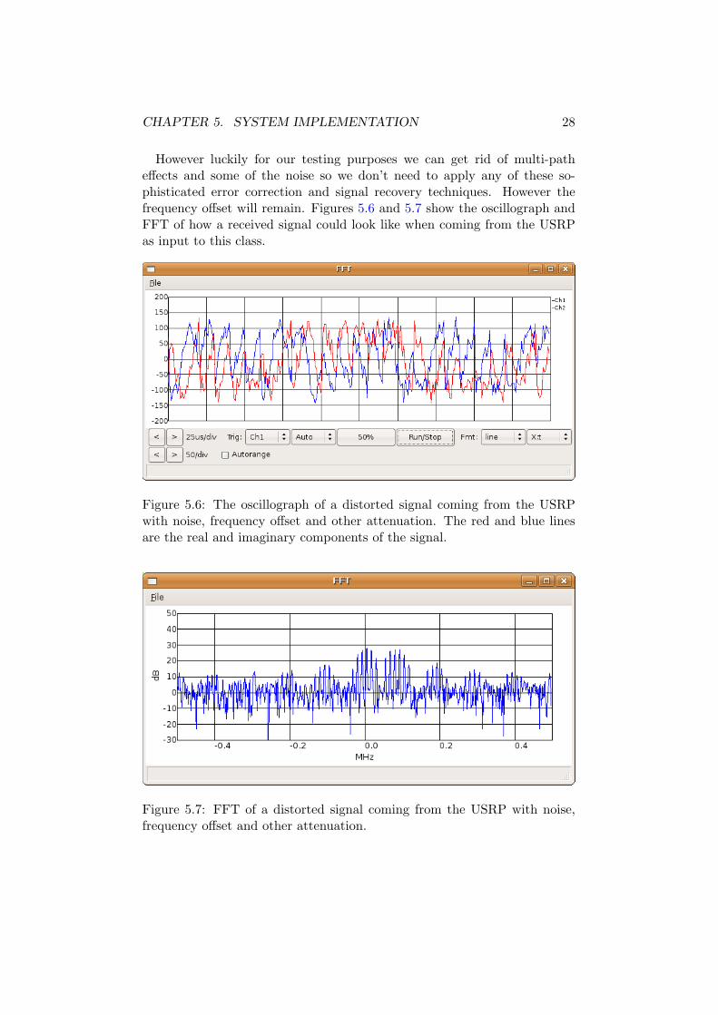
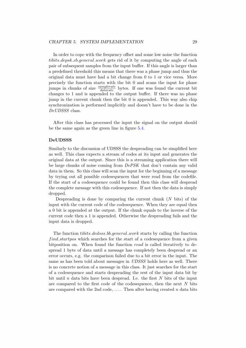
However luckily for our testing purposes we can get rid of multi-patheffects and some of the noise so we don’t need to apply any of these so-phisticated error correction and signal recovery techniques. However thefrequency offset will remain. Figures 5.6 and 5.7 show the oscillograph andFFT of how a received signal could look like when coming from the USRPas input to this class.

Figure 5.6: The oscillograph of a distorted signal coming from the USRPwith noise, frequency offset and other attenuation. The red and blue linesare the real and imaginary components of the signal.

Figure 5.7: FFT of a distorted signal coming from the USRP with noise,frequency offset and other attenuation.

CHAPTER 5. SYSTEM IMPLEMENTATION 29

In order to cope with the frequency offset and some low noise the functiontibits depsk cb.general work gets rid of it by computing the angle of eachpair of subsequent samples from the input buffer. If this angle is larger thana predefined threshold this means that there was a phase jump and thus theoriginal data must have had a bit change from 0 to 1 or vice versa. Moreprecisely the function starts with the bit 0 and scans the input for phasejumps in chunks of size samplerate

datarate bytes. If one was found the current bitchanges to 1 and is appended to the output buffer. If there was no phasejump in the current chunk then the bit 0 is appended. This way also chipsynchronization is performed implicitly and doesn’t have to be done in theDeUDSSS class.

After this class has processed the input the signal on the output shouldbe the same again as the green line in figure 5.4.

DeUDSSS

Similarly to the discussion of UDSSS the despreading can be simplified hereas well. This class expects a stream of codes at its input and generates theoriginal data at the output. Since this is a streaming application there willbe large chunks of noise coming from DePSK that don’t contain any validdata in them. So this class will scan the input for the beginning of a messageby trying out all possible codesequences that were read from the codefile.If the start of a codesequence could be found then this class will despreadthe complete message with this codesequence. If not then the data is simplydropped.

Despreading is done by comparing the current chunk (N bits) of theinput with the current code of the codesequence. When they are equal thena 0 bit is appended at the output. If the chunk equals to the inverse of thecurrent code then a 1 is appended. Otherwise the despreading fails and theinput data is dropped.

The function tibits dedsss bb.general work starts by calling the functionfind startpos which searches for the start of a codesequence from a givenbitposition on. When found the function read is called iteratively to de-spread 1 byte of data until a message has completely been despread or anerror occurs, e.g. the comparison failed due to a bit error in the input. Thesame as has been told about messages in UDSSS holds here as well. Thereis no concrete notion of a message in this class. It just searches for the startof a codesequence and starts despreading the rest of the input data bit bybit until n data bits have been despread. I.e. the first N bits of the inputare compared to the first code of the codesequence, then the next N bitsare compared with the 2nd code, . . . . Then after having created n data bits

CHAPTER 5. SYSTEM IMPLEMENTATION 30

(i.e. after successfully having processed n ·N input bits) the function startsagain by searching for the start of the next codesequence.

Comparing a chunk of N input bits with a code is done in the functionis code at which is the most central function of this class. It expects thepointer to the input buffer, the bitposition within the buffer to start thecomparison and a pointer to the code itself in its parameters. Then it startscomparing the input with the code (or its inverse) while taking care of thefact that the code can start at any position within the input and doesn’tnecessarily need to start at a full byte. That’s why the 2nd parameter is thebitposition within the input and not the byte position.

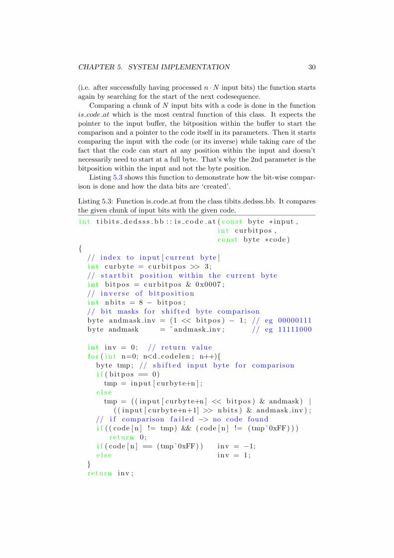
Listing 5.3 shows this function to demonstrate how the bit-wise compar-ison is done and how the data bits are ‘created’.

Listing 5.3: Function is code at from the class tibits dedsss bb. It comparesthe given chunk of input bits with the given code.

i n t t i b i t s d e d s s s b b : : i s c o d e a t ( const byte ∗ input ,i n t curb i tpos ,const byte ∗ code )

{// index to input [ cur rent byte ]i n t curbyte = curb i tpo s >> 3 ;// s t a r t b i t p o s i t i o n with in the cur rent bytei n t b i tpo s = curb i tpo s & 0x0007 ;// i n v e r s e o f b i t p o s i t i o ni n t nb i t s = 8 − b i tpo s ;// b i t masks f o r s h i f t e d byte comparisonbyte andmask inv = (1 << b i tpo s ) − 1 ; // eg 00000111byte andmask = ˜andmask inv ; // eg 11111000

i n t inv = 0 ; // return valuef o r ( i n t n=0; n<d code l en ; n++){

byte tmp ; // s h i f t e d input byte f o r comparisoni f ( b i tpo s == 0)

tmp = input [ curbyte+n ] ;e l s e

tmp = ( ( input [ curbyte+n ] << b i tpo s ) & andmask ) |( ( input [ curbyte+n+1] >> nb i t s ) & andmask inv ) ;

// i f comparison f a i l e d −> no code foundi f ( ( code [ n ] != tmp) && ( code [ n ] != (tmpˆ0xFF) ) )

re turn 0 ;i f ( code [ n ] == (tmpˆ0xFF) ) inv = −1;e l s e inv = 1 ;

}re turn inv ;

CHAPTER 5. SYSTEM IMPLEMENTATION 31

}

After passing this block the original data should be restored completelyagain and can be passed to the receiver.

Receiver Appl

Finally after demodulation and despreading the Receiver Appl can bufferthe messages, verify the checksums and perform time measurement.

More precisely it expects data in form of messages as defined in figure5.2. So it scans the input for the unique package header to find the startof a new package. When found it extracts the message id and package idfields, buffers the payload data and crc performs a checksum verificationand if successful stores the received message locally and stores the measuredtimes.

Every time when the main function tibits appl receiver.general work iscalled it sits in one of three states: Either there is no current message, soit’ll search for the start of a new message in the input buffer which is donein the function find pck start. Or it’s currently buffering payload data orit’s storing and verifying the crc.

When a message was successfully received the time is stored locally andwritten to standard output (or a file) to allow further statistics over theprocessing performance.

5.4 Summary

In this chapter the reader saw how the data is created and how it flowsthrough the system. We saw how the different sender and receiver blocksprocess the data, how the signal changes after each block and how we caneasily cope with such things as frequency offset and noise. All these expla-nations were backed up by illustrative examples, figures and code listings.

Now let’s have a look at the system in action when explaining the ex-periments, measurements and the testbed layout.

Part III

Experiments andConclusions

32

Chapter 6

Experiments andMeasurements

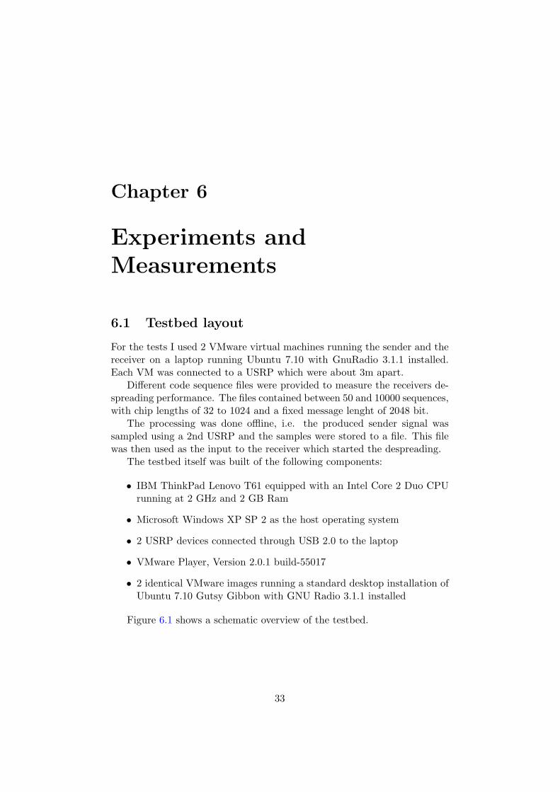
6.1 Testbed layout

For the tests I used 2 VMware virtual machines running the sender and thereceiver on a laptop running Ubuntu 7.10 with GnuRadio 3.1.1 installed.Each VM was connected to a USRP which were about 3m apart.

Different code sequence files were provided to measure the receivers de-spreading performance. The files contained between 50 and 10000 sequences,with chip lengths of 32 to 1024 and a fixed message lenght of 2048 bit.

The processing was done offline, i.e. the produced sender signal wassampled using a 2nd USRP and the samples were stored to a file. This filewas then used as the input to the receiver which started the despreading.

The testbed itself was built of the following components:

• IBM ThinkPad Lenovo T61 equipped with an Intel Core 2 Duo CPUrunning at 2 GHz and 2 GB Ram

• Microsoft Windows XP SP 2 as the host operating system

• 2 USRP devices connected through USB 2.0 to the laptop

• VMware Player, Version 2.0.1 build-55017

• 2 identical VMware images running a standard desktop installation ofUbuntu 7.10 Gutsy Gibbon with GNU Radio 3.1.1 installed

Figure 6.1 shows a schematic overview of the testbed.

33

CHAPTER 6. EXPERIMENTS AND MEASUREMENTS 34

Figure 6.1: The testbed used for the measurements. Sender and receiverare 3m apart and each connected over USB to a laptop that is running 2VMware machines simultaneously.

CHAPTER 6. EXPERIMENTS AND MEASUREMENTS 35

6.2 Test cases

Since the system is meant as a proof of concept for the U-DSSS scheme themain interest was to measure the time used by the receiver to despread thesignal. Based on this the following criteria were defined:

1. Minimal, maximal and average time to despread the first bit of amessage

2. Min, max and avg time to despread the whole message after the firstbit was found

Let me quickly explain what these values mean. The first bit time isthe time used by the receiver from start of the application to when the firstbit could successfully be despread. So the incoming data that is read fromthe file is searched for any occurrence of a valid first code of one of thedefined codesequences. If such a code could be found in the input then thistime is measured, independently of the successful despreading of the wholemessage. Thus this time stands for the processing time that is used by thefunctions to search through the input buffer plus the time used by the GNURadio framework to call and run the blocks, e.g. to copy output buffersfrom preceding blocks to input buffers of the current block.

The second value message time on the other hand stands really for twovalues. Firstly the processing time used by the block DeUDSSS to despreada whole message, i.e. to compare the codes from the codesequence bit bybit with the input, after the first bit was found. This is purely based onthe speed of the CPU and the length of the message. Secondly as first bittime it also depends on how fast the GNU Radio framework handles thebuffering.

All tests were repeated between 20 and 100 times in order to get mean-ingful average times and min-max intervals. However since running on Win-dows the time granularity was restricted to 10ms. Also a lot of the time thatis measured is not coming from the system itself but, as we will see in thenext section, from the framework that e.g. needs time to read the sampleddata from the input file, create and handle buffering between the blocks, . . .

6.3 Results

What follows are some of the charts that were generated out of the exhaus-tive test data.

6.3.1 First bit times per Nr. of Codesequences

Figures 6.2 and 6.3 compare the first bit times and their min-max intervalsfor different ks (number of codesequences) and code bitlengths of 32 or 1024

CHAPTER 6. EXPERIMENTS AND MEASUREMENTS 36

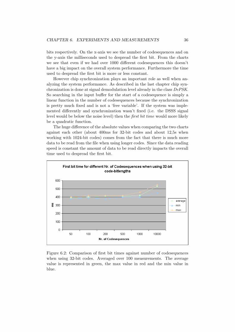
bits respectively. On the x-axis we see the number of codesequences and onthe y-axis the milliseconds used to despread the first bit. From the chartswe see that even if we had over 1000 different codesequences this doesn’thave a big impact on the overall system performance. Furthermore the timeused to despread the first bit is more or less constant.

However chip synchronization plays an important role as well when an-alyzing the system performance. As described in the last chapter chip syn-chronization is done at signal demodulation level already in the class DePSK.So searching in the input buffer for the start of a codesequence is simply alinear function in the number of codesequences because the synchronizationis pretty much fixed and is not a ‘free variable’. If the system was imple-mented differently and synchronization wasn’t fixed (i.e. the DSSS signallevel would be below the noise level) then the first bit time would more likelybe a quadratic function.

The huge difference of the absolute values when comparing the two chartsagainst each other (about 400ms for 32-bit codes and about 12,5s whenworking with 1024-bit codes) comes from the fact that there is much moredata to be read from the file when using longer codes. Since the data readingspeed is constant the amount of data to be read directly impacts the overalltime used to despread the first bit.

Figure 6.2: Comparison of first bit times against number of codesequenceswhen using 32-bit codes. Averaged over 100 measurements. The averagevalue is represented in green, the max value in red and the min value inblue.

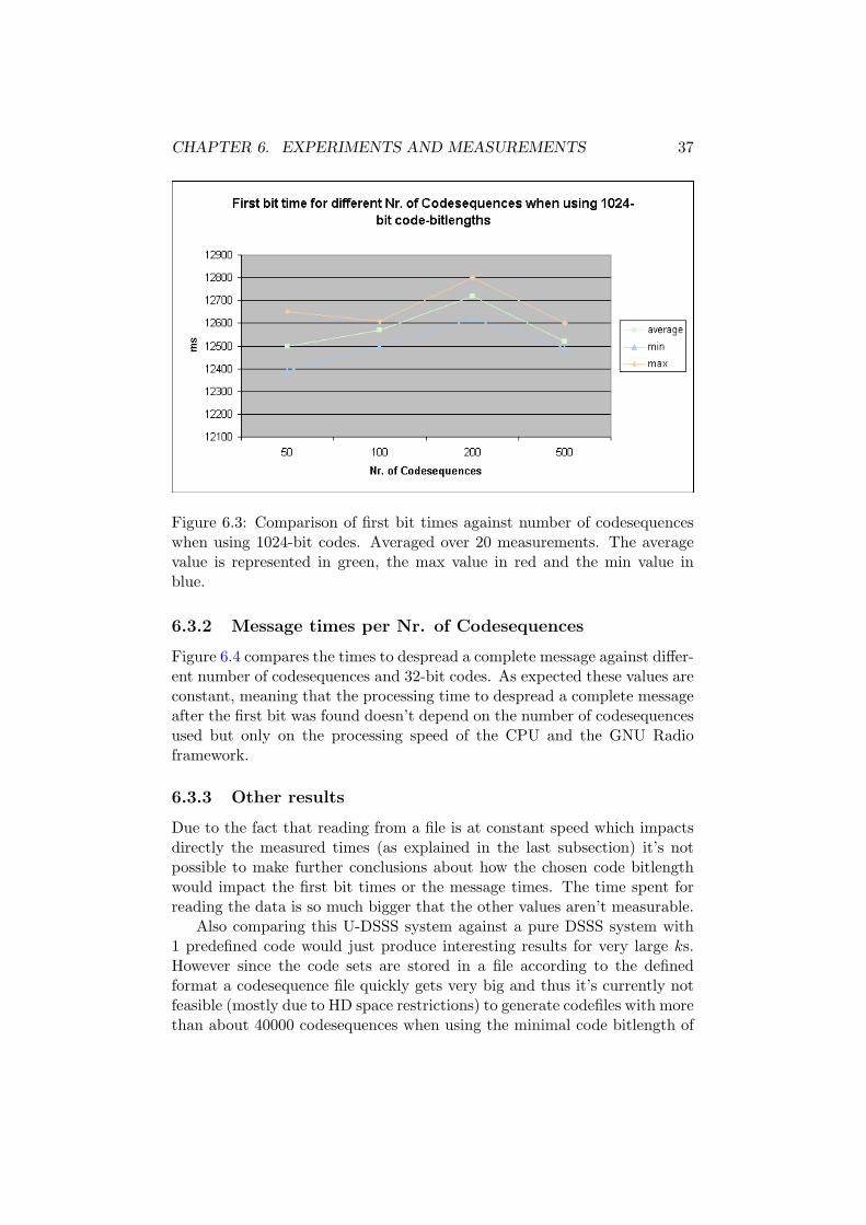
CHAPTER 6. EXPERIMENTS AND MEASUREMENTS 37

Figure 6.3: Comparison of first bit times against number of codesequenceswhen using 1024-bit codes. Averaged over 20 measurements. The averagevalue is represented in green, the max value in red and the min value inblue.

6.3.2 Message times per Nr. of Codesequences

Figure 6.4 compares the times to despread a complete message against differ-ent number of codesequences and 32-bit codes. As expected these values areconstant, meaning that the processing time to despread a complete messageafter the first bit was found doesn’t depend on the number of codesequencesused but only on the processing speed of the CPU and the GNU Radioframework.

6.3.3 Other results

Due to the fact that reading from a file is at constant speed which impactsdirectly the measured times (as explained in the last subsection) it’s notpossible to make further conclusions about how the chosen code bitlengthwould impact the first bit times or the message times. The time spent forreading the data is so much bigger that the other values aren’t measurable.

Also comparing this U-DSSS system against a pure DSSS system with1 predefined code would just produce interesting results for very large ks.However since the code sets are stored in a file according to the definedformat a codesequence file quickly gets very big and thus it’s currently notfeasible (mostly due to HD space restrictions) to generate codefiles with morethan about 40000 codesequences when using the minimal code bitlength of

CHAPTER 6. EXPERIMENTS AND MEASUREMENTS 38

Figure 6.4: Comparison of message times against number of codesequenceswhen using 32-bit codes. Averaged over 100 measurements. The averagevalue is represented in green, the max value in red and the min value inblue.

8-bit codes.So for further tests with this system it would be interesting to implement

another codefile format and time measurements that don’t depend on thespeed of how fast the data is read.

Chapter 7

Conclusions

7.1 Review

The aim of my master thesis was to design and implement a system for Un-coordinated Direct Sequence Spread Spectrum (U-DSSS). This documentstarted by explaining the necessary backgrounds like the GNU Radio frame-work and added a short introduction to what we need to know about digitalsignal processing. We saw what a common SDR application looks like, whata RF front end is and the corresponding parts of it in the GNU Radio world.We also learned what digital filters are and how to write and link them inGNU Radio.

Then this report proceeded to define the system implementation startingwith a quick overview that showed the system on the whole and then goinginto details, explaining each block in detail. There we saw the sender andthe receiver flowgraphs and how they communicate with each other overUSRPs. Also how spreading and modulation is done in the digital worldand what needs to be considered when a signal passes over the air and getsdistorted. Where necessary, the design decisions were explained and whycertain things were implemented this way and not the other. Finally afterevery block we followed the pathway of a data signal that flows through thesystem shown with illustrative figures.

In the third part we saw the system in action. The testbed was defined,test cases were generated and finally the produced results were illustratedwith graphs.

7.2 Lessons learned

The project started with evaluating different platforms that could be usedto implement the proposed system. Choosing an open source solution, GNURadio, was generally a good choice because it leaves very much freedom ofwhat the implementation finally will look like. Also it didn’t restrict me in

39

CHAPTER 7. CONCLUSIONS 40

any sense such that there would have been something that wasn’t possibleto implement. Although I sometimes had to work around some limitationslike the fact that the framework is purely stream-based and thus doesn’tprovide a simple way for the different blocks to exchange control data.

However spending more time in evaluating other systems could have beeninteresting. Especially when considering performance issues hardware basedsystems that already provide basic DSSS functionality would be interestingto work with.

But after all I found GNU Radio to be very easy and great fun to use soI’ll surely do further projects with it in the future.

7.2.1 Project management

During the project a lot has changed (see the project schedule in the ap-pendix). For a next project I’d certainly concentrate more on projectmanagement, i.e. planning, designing, thinking about the proposed ideas,scheduling more meetings with the ‘customers’ in order to get a clearer viewof what the final system should look like. However due to the fact thatthe ‘idea’ of the final system evolved as well during the project, this wasn’tnecessarily possible this time.

7.3 Future work

The current system was implemented as a proof of concept only. Thus manydesign choices were made in order to get fast and reliable results. Althoughit provides everything that we defined to be absolutely necessary for thefirst version there’s certainly much more that could have been done withU-DSSS.

Here are just a few of the many examples of what further developmentcould look like:

• One of the major characteristics of DSSS is that the signal ‘hides’below the noise level and thus is not visible to the attacker. For thecurrent implementation of DePSK to work, the signal must however bestronger than the noise. Extending this implementation would makethe system more secure. Although it would also have a big impacton the system performance because chip synchronization couldn’t bedone at PSK stage anymore but would have to be done at the DSSSlevel.

• Currently the system can only recognize one sender and processes theinput stream only one time in order to find the strongest signal. Fur-ther development would need to be done to recognize multiple sendersthat overlap each other using different codesequences.

CHAPTER 7. CONCLUSIONS 41

• Error correction and signal recovery mechanisms could be appliedwhen the signal enters the system in order to make it more robustto noise and signal distortion. These mechanisms could consist of chiptiming recovery, carrier signal synchronization, application of matchedfilters, . . .

• Having a more robust system, different attacker models can be imple-mented to get a better insight of how an attacker can harm the systemperformance.

• Support fragmentation of a message, i.e. split a message into packetsof same length and spread each packet with an own codesequence.

• Improving the time measurements to get closer to the time that reallyis spent by the system.

• Implement the key exchange protocol that is propsed in [1] and let itrun against the different attacker models.

However probably the most interesting enhancement to this system wouldbe to implement it ‘in-the-small’. Where ‘in-the-small’ means that it’s eitherintegrated into small devices or provides an open easy to use interface suchthat other systems can seamlessly use it without having to make a lot ofchanges. This solution would allow other systems to easily bootstrap theirjamming-resistant communication by exchanging keys or other informationusing U-DSSS.

Part IV

Appendix

42

Appendix A

Project Schedule

A.1 Review

Due to the nature of the project it was clear at project start that it wasn’tpossible to define a fixed project schedule. I still tried to define at least themost important milestones and some rough key-dates in order to have anoverview of what steps will lead to the final system.

During the project evolvement a lot has changed, rendering the originaldates mostly useless. E.g. the implementation changed from UFH to U-DSSS, also the measurements, results and some extensions to the systembecame more important than a sophisticated attacker model, so that thisand other milestones got dropped.

However I think it’s important to see and analyse the differences betweenthe planned and the actual schedule of any project in order to learn for futureprojects and to improve.

A.2 Planned schedule

The first meeting was on Wed, 19th of Sept 2007 where we decided aboutmy master thesis topic and fixed an official starting date, the 8th of October2007.

Figure A.1 is a mind map that shows the different planned steps, thedefined milestones and the rough due dates. This map was created rightafter our kickoff meeting on Oct 10, 2007.

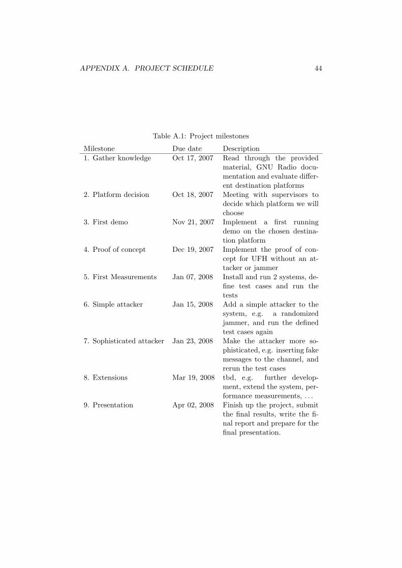
Table A.1 explains the defined milestones in more detail.

A.3 Actual schedule

After the first 3 defined milestones were reached the project plan changedand we defined new objectives that rendered the old milestones invalid. Sothe actual project schedule looked as follows:

43

APPENDIX A. PROJECT SCHEDULE 44

Table A.1: Project milestones

Milestone Due date Description1. Gather knowledge Oct 17, 2007 Read through the provided

material, GNU Radio docu-mentation and evaluate differ-ent destination platforms

2. Platform decision Oct 18, 2007 Meeting with supervisors todecide which platform we willchoose

3. First demo Nov 21, 2007 Implement a first runningdemo on the chosen destina-tion platform

4. Proof of concept Dec 19, 2007 Implement the proof of con-cept for UFH without an at-tacker or jammer

5. First Measurements Jan 07, 2008 Install and run 2 systems, de-fine test cases and run thetests

6. Simple attacker Jan 15, 2008 Add a simple attacker to thesystem, e.g. a randomizedjammer, and run the definedtest cases again

7. Sophisticated attacker Jan 23, 2008 Make the attacker more so-phisticated, e.g. inserting fakemessages to the channel, andrerun the test cases

8. Extensions Mar 19, 2008 tbd, e.g. further develop-ment, extend the system, per-formance measurements, . . .

9. Presentation Apr 02, 2008 Finish up the project, submitthe final results, write the fi-nal report and prepare for thefinal presentation.

APPENDIX A. PROJECT SCHEDULE 45

Figure A.1: Original project schedule including milestones. Generated usingMindManager.

Table A.2 explains the actual schedule along with the due and meetingdates.

APPENDIX A. PROJECT SCHEDULE 46

Table A.2: The actual project schedule

Until Description1. Oct 17, 2007 Read through the provided material, GNU Radio doc-

umentation and evaluate different destination plat-forms

2. Oct 18, 2007 Meeting with supervisors to decide which platform wewill choose. Decision: GNU Radio with 2 USRPs.

3. Dec 3, 2007 Presentation of the first tests and implementationswith GNU Radio. Meeting date was shifted from Nov29 due to timing collisions. Objectives changed: Wewill implement a system for U-DSSS instead of UFH.The exact conditions will follow.

4. Dec 12, 2007 Meeting with Prof. Dr. Capkun and supervisors dis-cussing open questions concerning DSP, FFT, . . . Pre-liminary definition of what the minimal requirementsfor a system are that will suffice as a proof of conceptfor U-DSSS.

5. Jan 16, 2008 Meeting with Prof. Dr. Capkun and supervisorsshowing a first prelimiary presentation of the imple-mented system. [DRAFT] The presentation slides canbe found in the appendix.

6. Jan 18, 2008 Delivery of a VMware image that contains the currentsystem running on Ubuntu.

7. Feb 13, 2008 Enhancements to the system and implementation ofsender and receiver application to support time mea-surements, crc, . . .

8. Feb 18, 2008 First definition of test cases and measurements.9. Mar 05, 2008 Final definition of test cases, start running the test and

produce the results for Christinas and Marios paperabout U-DSSS.

10. Mar 12, 2008 Delivery of test results and system short description.11. Apr 8, 2008 Enhancements to the system. Deadline for the final

master thesis report.

Appendix B

Preliminary presentation Jan16, 2008

47

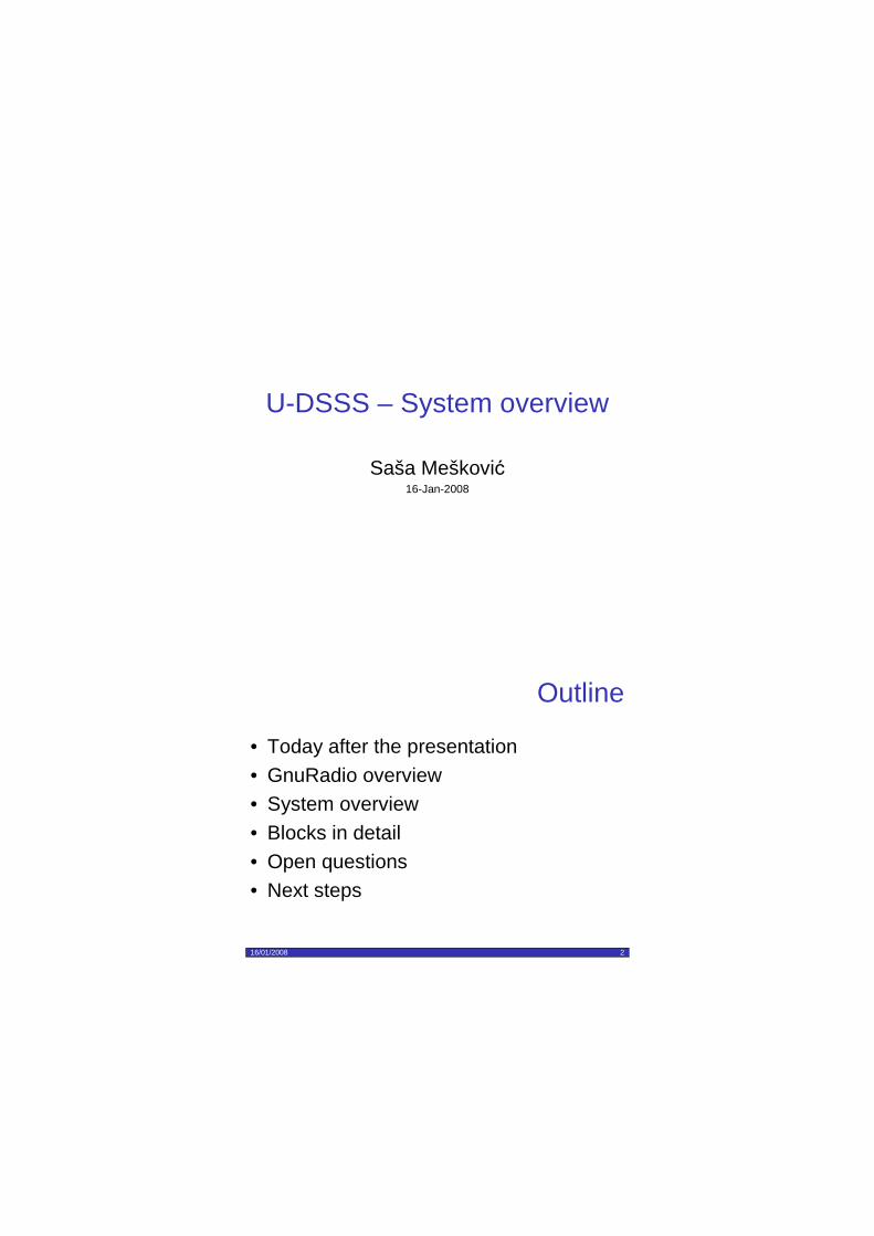
U-DSSS – System overview

Saša Mešković16-Jan-2008

16/01/2008 2

Outline

• Today after the presentation• GnuRadio overview• System overview• Blocks in detail• Open questions• Next steps

16/01/2008 3

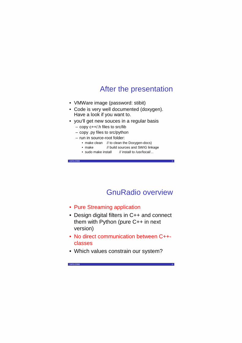
After the presentation

• VMWare image (password: stibit)• Code is very well documented (doxygen).

Have a look if you want to.• you‘ll get new souces in a regular basis

– copy c++/.h files to src/lib– copy .py files to src/python– run in source-root folder:

• make clean // to clean the Doxygen-docs)• make // build sources and SWIG linkage• sudo make install // install to /usr/local/...

16/01/2008 4

GnuRadio overview

• Pure Streaming application• Design digital filters in C++ and connect

them with Python (pure C++ in next version)

• No direct communication between C++-classes

• Which values constrain our system?

16/01/2008 5

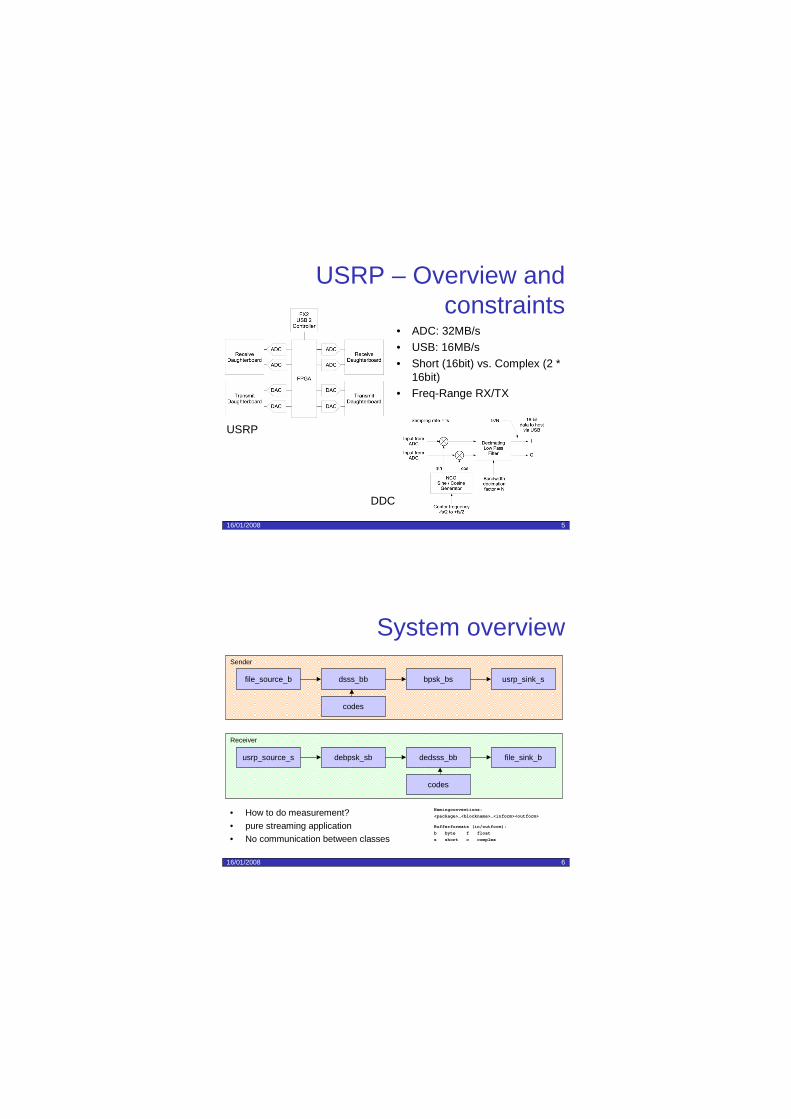
USRP – Overview and constraints

• ADC: 32MB/s• USB: 16MB/s• Short (16bit) vs. Complex (2 *

16bit)• Freq-Range RX/TX

USRP

DDC

16/01/2008 6

System overview

• How to do measurement?• pure streaming application• No communication between classes

Bufferformats (in/outform):b byte f floats short c complex

Namingconventions:<package>_<blockname>_<inform><outform>

Sender

file_source_b dsss_bb bpsk_bs usrp_sink_s

codes

Receiver

debpsk_sbusrp_source_s dedsss_bb file_sink_b

codes

16/01/2008 7

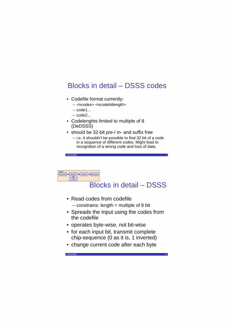
Blocks in detail – DSSS codes

• Codefile format currently:– <ncodes> <ncodebitlength>– code1...– code2...

• Codelenghts limited to multiple of 8 (DeDSSS)

• should be 32-bit pre-/ in- and suffix free– i.e. it shouldn't be possible to find 32 bit of a code

in a sequence of different codes. Might lead to recognition of a wrong code and loss of data.

16/01/2008 8

Blocks in detail – DSSS

• Read codes from codefile– constrains: length = multiple of 8 bit

• Spreads the input using the codes from the codefile

• operates byte-wise, not bit-wise• for each input bit, transmit complete

chip-sequence (0 as it is, 1 inverted)• change current code after each byte

Sender

file_source_b dsss_bb bpsk_bs usrp_sink_s

codes

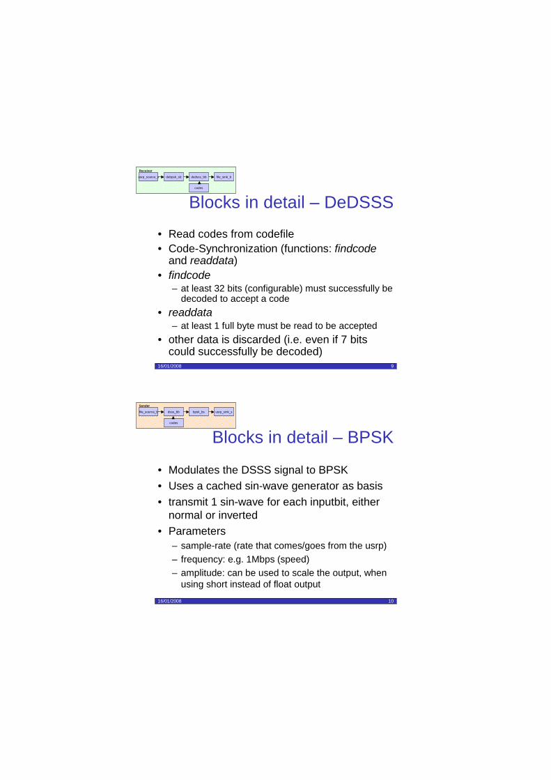
16/01/2008 9

Blocks in detail – DeDSSS

• Read codes from codefile• Code-Synchronization (functions: findcode

and readdata)• findcode

– at least 32 bits (configurable) must successfully be decoded to accept a code

• readdata– at least 1 full byte must be read to be accepted

• other data is discarded (i.e. even if 7 bits could successfully be decoded)

Receiver

debpsk_sbusrp_source_s dedsss_bb file_sink_b

codes

16/01/2008 10

Blocks in detail – BPSK

• Modulates the DSSS signal to BPSK• Uses a cached sin-wave generator as basis• transmit 1 sin-wave for each inputbit, either

normal or inverted• Parameters

– sample-rate (rate that comes/goes from the usrp)– frequency: e.g. 1Mbps (speed)– amplitude: can be used to scale the output, when

using short instead of float output

Sender

file_source_b dsss_bb bpsk_bs usrp_sink_s

codes

16/01/2008 11

Blocks in detail - DeBPSK

• Converts modulated signal to bit-stream• Based on a cached sin-wave generator• Use ‚Zero-Search‘ to synchronize local sin-

wave with signal in the inputstream• Multiply local sin-wave with inputstream• current version has some bit errors with

average noiseàneeds further discussionàHow to synchronize with lower oversamplingàcould a ‚trainingsequence‘ help? à no insecure

Receiver

debpsk_sbusrp_source_s dedsss_bb file_sink_b

codes

16/01/2008 12

A few examples ...

16/01/2008 13

Open questions & next steps

• DeBPSK issues• How to integrate this streaming blocks into an

‚application‘ with time measurement, crc, ... ?

àEvaluate QPSK (native GnuRadio)àFeedback from lower blocks to DeBPSKàIntegrate all receiver blocks into 1 class à

similar to offline processing

Bibliography

[1] Mario Strasser and Christina Popper. Jamming-resistant Key Estab-lishment using Uncoordinated Frequency Hopping. In Proceedings ofIEEE Symposium on Security and Privacy, 2008, to appear.

[2] Christina Popper and Mario Strasser. Uncoordinated Direct SequenceSpread Spectrum. Not yet published.

[3] GNU Radio homepage http://gnuradio.org/trac/

[4] Eric Blossom. Exploring GNU Radio. http://www.gnu.org/software/gnuradio/doc/exploring-gnuradio.html

[5] Eric Blossom. How to Write a Signal Processing Block. http://www.gnu.org/software/gnuradio/doc/howto-write-a-block.html

[6] J. Nicholas Laneman. SDR Documentation. http://www.nd.edu/

~jnl/sdr/docs/

[7] Eric Blossom. Listening to FM Radio in Software, Step by Step. http://www.linuxjournal.com/article/7505

[8] Ettus Research LLC http://www.ettus.com/

[9] USRPv4 specification: A flexible, extensible RF front end mainly de-veloped for use with GNU Radio. http://www.ettus.com/downloads/usrp_v4.pdf

[10] Preliminary binary installers for GNU Radio on Windows.http://www.olifantasia.com/projects/gnuradio/mdvh/mingw/binary-installer/gnuradio-with-usrp/

[11] Virtualization software for most current operating systems. VMwarehomepage http://www.vmware.com/

[12] Community developed, Linux-based operating system. Ubuntu home-page http://www.ubuntu.com/

[13] Python online tutorial http://www.python.org/doc/current/tut/

55

BIBLIOGRAPHY 56

[14] Dive Into Python http://www.diveintopython.org/

[15] Short DSP tutorial http://www.dsptutor.freeuk.com/

[16] dspGuru. Digital Signal Processing Central. http://www.dspguru.com/

[17] Bores signal processing. Introduction to DSP. http://www.bores.com/courses/intro/

[18] Steven W. Smith. The Scientist and Engineer’s Guide to Digital SignalProcessing. http://www.dspguide.com/

[19] John G. Proakis. Digital Communications. ISBN-10: 0071181830,ISBN-13: 978-0071181839. http://www.mhhe.com/engcs/electrical/proakis/

[20] Doxygen. Source code documentation generator tool. http://www.doxygen.org/