Right Whale Vessel Speed Economic Analysis

IEc

Economic Analysis of the North

Atlantic Right Whale Vessel Speed

Restriction Rule

March 2020

Prepared for:

Office of Protected Resources

National Marine Fisheries Service

1315 East-West Highway, SSMC III

Silver Spring, MD 20910

Prepared by:

Industrial Economics, Incorporated

2067 Massachusetts Avenue

Cambridge, MA 02140

617/354-0074

i

TABLE OF CONTENTS

EXECUTIVE SUMMARY

CHAPTER 1 | INTRODUCTION

Overview of Rule 1-1

Previous Economic Analyses 1-6

2008 Analysis 1-6

2012 Analysis 1-6

Scope of this Analysis 1-7

CHAPTER 2 | IMPACTS ON TRANSIT TIME

Introduction 2-1

Data Sources 2-1

AIS Data 2-1

Data Processing and Screening 2-1

Overview of Analysis Data Set 2-3

Analysis of Transit Speeds 2-3

Calculation of Impacts on Transit Times 2-8

Overview of Methods 2-8

Method 1: Comparison of Means 2-9

Method 2: Comparison of High-Speed Transits 2-10

Summary 2-16

CHAPTER 3 | ANNUAL COST IMPACTS

Introduction 3-1

Hourly Vessel Operating Costs: Caveats and Limitations 3-1

Commercial Shipping Vessels 3-3

Hourly Operating Costs 3-3

Fuel Costs 3-5

Fuel Consumption 3-5

Application of Fuel Consumption Equations 3-7

Fuel Prices 3-8

Limitations 3-9

Annual Cost Impacts 3-9

Passenger Cruise Ships 3-10



ii

Fishing Vessels 3-14


Non-Labor Costs 3-15

Labor Costs 3-15

Total Hourly Costs 3-16

Estimation of Operating Cost Models 3-16


Towing/Pushing Vessels 3-18



Dredging Vessels 3-20



Other (Non-Cruise) Passenger Vessels 3-22



Limitations 3-23

Pleasure Craft 3-24

Other Vessels 3-24



Summary 3-25

CHAPTER 4 | CONSIDERATION OF BROADER ECONOMIC IMPACTS

Introduction 4-1

Port Calls 4-1

Import/Export Values 4-3

Summary 4-5

CHAPTER 5 | CONCLUSIONS

Principal Findings 5-1

Limitations and Uncertainties 5-1

Potential Refinements and Additional Applications 5-2

APPENDIX A | ADDITIONAL STATISTICS ON SMA TRANSITS

APPENDIX B | IMPACTS ASSUMING FULL COMPLIANCE

APPENDIX C | NOTES ON ESTIMATES OF VESSEL OPERATING COSTS

REFERENCES

ES-1

EXECUTIVE SUMMARY

In accordance with the requirements of 50 CFR § 224.105(d), the National Oceanic and Atmospheric

Administration (NOAA) has initiated an assessment of the costs and benefits of the vessel speed

limitations set forth in the Final Rule to Implement Speed Restrictions to Reduce the Threat of Ship

Collisions with North Atlantic Right Whales. In support of this effort, Industrial Economics, Incorporated

(IEc) is working with the Office of Protected Resources of the National Marine Fisheries Service (NMFS)

to analyze the Rule’s costs. This report presents our findings. It begins with an analysis of vessel transit

data to assess the marginal effect of the Rule on transit times, i.e., the extent to which transits through

areas subject to the Rule are delayed when vessels reduce their speed to comply with its requirements. It

then applies available data on hourly operating costs for various types of vessels to estimate the direct

costs attributable to these delays.

Depending on the method employed to characterize the Rule’s impact on transit times, we estimate its

direct costs at approximately $28.3 million to $39.4 million annually. The analysis indicates that the

commercial shipping industry bears between 74 to 87 percent of these costs. This result is not surprising.

Of the wide range of vessels the Rule affects, commercial shipping accounts for the greatest number of

affected transits. These vessels also have high hourly operating costs and ordinarily operate at relatively

high speeds; thus, the impact of the speed restrictions on their operations accounts for a large share of the

costs attributable to the Rule. In comparison, other types of vessels account for a substantially smaller

share of the Rule’s estimated costs, either because their hourly operating costs and/or routine operating

speeds are much lower – as is the case with commercial fishing vessels – or because they account for a

smaller share of affected transits.

Our analysis is subject to several important limitations. Most notably, the data available on vessel

operating costs are limited, and the characterization of the counterfactual scenario upon which our

estimates are based – i.e., our estimate of the speed at which vessels would operate in the absence of the

Rule – involves some degree of professional judgment. Additionally, our analysis considers only the

direct costs of the Rule; we do not attempt to evaluate the extent to which these costs may be passed on to

consumers in the form of higher prices, nor do we attempt to analyze the potential effect of changes in

operating costs on overall levels of commercial shipping activity. We do, however, briefly review the

available data on commercial shipping activity since the Rule took effect. This review provides no prima

facie evidence that the Rule has had an adverse effect on the volume or value of economic activity at

ports along the eastern seaboard.

1-1

CHAPTER 1 | INTRODUCTION

OVERVIEW OF RULE

The North Atlantic right whale (Eubalaena glacialis) is one of the world’s most endangered large whale

species, having been hunted by commercial whalers over many decades to the brink of extinction. The

species has been protected from whaling since 1935, and in 1970 was listed as endangered under the U.S.

Endangered Species Act. Despite these and other efforts to protect right whales, the species has failed to

recover. Current estimates place the remaining population at approximately 400 individuals.1

Recent efforts to restore the population of the North Atlantic right whale have focused on reducing the

number of deaths and injuries attributable to anthropogenic causes. This includes reducing the likelihood

and severity of vessel strikes – collisions between vessels and whales – which have been identified as one

of the leading causes of right whale mortality. The potential for a vessel strike is likely to be higher

where busy transit corridors intersect with important right whale habitat.

Research on vessel strikes has shown that both their likelihood and severity increase with vessel speed.

Guided by these findings, NMFS aims to protect right whales from vessel strikes by restricting vessel

operating speeds in areas where right whales are likely to be found. These restrictions first took effect in

2008, when NMFS published a “Final Rule to Implement Speed Restrictions to Reduce the Threat of Ship

Collisions with North Atlantic Right Whales” (we refer to the 2008 Final Rule, collectively with its

modifications, as the “Rule”).2 The objective of the Rule is to facilitate the recovery of the right whale by

requiring certain oceangoing vessels to travel at speeds of 10 knots or less at specific times and locations,

known as Seasonal Management Areas (SMAs), where right whales are likely to be found. In addition to

establishing SMAs, the Rule provides for the establishment of Dynamic Management Areas (DMAs) at

locations and times in which aggregations of right whales outside SMAs are detected. DMAs are

established as needed, generally for a period of 15 days, though they can be extended if whales remain in

the area. Vessel operators are requested, but not required, to avoid DMAs or to transit DMAs at speeds no

greater than 10 knots.

With certain exceptions, all vessels greater than or equal to 65 feet in overall length and subject to the

jurisdiction of the United States, as well as all vessels greater than 65 feet entering or departing a U.S.

port or place, are subject to the speed restrictions while traveling through SMAs.3 Vessels greater than or

equal to 65 feet in length that are not subject to the Rule include vessels owned or operated by the Federal

1 https://www.fisheries.noaa.gov/species/north-atlantic-right-whale.

2 “Endangered Fish and Wildlife; Final Rule to Implement Speed Restrictions to Reduce the Threat of Ship Collisions with North Atlantic Right

Whales,” 73 Federal Register 60173 (December 9, 2008), 50 CFR Part 224.

3 Compliance Guide for Right Whale Ship Strike Reduction Rule 950 CFR 224.105), National Marine Fisheries Service.

https://www.fisheries.noaa.gov/species/north-atlantic-right-whale

1-2

government; U.S. military vessels; foreign military vessels while engaged in exercises with the U.S.

Navy; and active state law enforcement/rescue vehicles.

Table 1-1 identifies the 10 SMAs established under the Rule and the dates the speed restrictions are in

effect. Figure 1-1, Figure 1-2, and Figure 1-3 show the location of the SMAs in the Northeast, Mid-

Atlantic, and Southeast regions.

TABLE 1 -1. SEASONAL MANAGEMENT AREAS

REGION NAME SHORTHAND NAME EFFECTIVE DATES

PERCENT OF YEAR

IN EFFECT

Northeast

Cape Cod Bay Cape Cod Bay January 1 - May 15

37%

Off Race Point Off Race Point March 1 - April 30 17%

Great South Channel Great South Channel April 1 - July 31 33%

Mid-Atlantic

Block Island Sound Block Island

November 1 - April 30

50%

Ports of New York/New Jersey

New York

Entrance to the Delaware Bay (Ports of Philadelphia and Wilmington)

Philadelphia

Entrance to the Chesapeake Bay (Ports of Hampton Roads and Baltimore)

Norfolk

Ports of Morehead City and Beaufort, NC

Morehead City

Wilmington, NC, to Brunswick, GA

North Carolina to Georgia

Southeast Calving and Nursery Grounds

Southeast November 15 - April 15

42%

1-3

FIGURE 1-1. NORTHEAST SEASONAL MANAGEMENT AREAS 4

4 “Reducing Ship Strikes to North Atlantic Right Whales,” NOAA Fisheries, accessed at https://www.fisheries.noaa.gov/national/endangered-

species-conservation/reducing-ship-strikes-north-atlantic-right-whales.

https://www.fisheries.noaa.gov/national/endangered-species-conservation/reducing-ship-strikes-north-atlantic-right-whales


1-4

FIGURE 1-2. MID-ATLANTIC SEASONAL MANAGEMENT AREAS 5





1-5

FIGURE 1-3. SOUTHEAST SEASONAL MANAGEMENT AREAS 6





1-6

PREVIOUS ECONOMIC ANALYSES

2008 ANALYSIS

In support of the 2008 Rule, Nathan Associates Inc. prepared a prospective analysis of its potential

economic impacts.7 In its analysis, Nathan Associates estimated the potential economic impacts

associated with six different combinations of four operational measures (recommended routes; SMAs;

DMAs; and speed restrictions) designed to reduce the frequency and severity of vessel strikes to right

whales. The preferred alternative in this analysis closely aligns with – but is not identical to – the final

Rule.8

Nathan Associates’ economic impact assessment was based on estimates of the delay vessels would

experience by complying with the proposed speed restrictions, coupled with information on typical vessel

operating costs.9 Notably, Nathan Associates estimated delays under an assumption of full compliance

with the Rule; i.e., an assumption that all vessels subject to the rule would reduce their speeds to the

proposed statutory limit. Nathan Associates estimated delays using Mandatory Ship Reporting System

data (which provides actual operating speeds reported by ship captains) and U.S. Army Corps of

Engineers (USACE) operating cost data (which include annualized capital costs, estimates of fixed

operating costs, and fuel costs at sea and in port).10

Nathan Associates estimated a wide range of economic impacts to the commercial shipping industry, with

annual impacts under the preferred alternative of approximately $53 million.11 Nathan Associates

estimated substantially lower impacts to commercial fishing, charter fishing, passenger ferry, and whale

watching vessels.12

2012 ANALYSIS

Nathan Associates conducted a retrospective economic analysis of the Rule in 2012.13 The methodology

employed in this analysis was similar to that used in Nathan Associates’ 2008 analysis; i.e., calculating

the impact of the Rule on travel time, then estimating the associated increase in operating costs. In this

case, however, the estimate of impacts on the commercial shipping industry was based on observations of

vessel operations within the SMAs, as recorded by the U.S. Coast Guard Automatic Identification System

(AIS). AIS uses transmitters to relay a vessel’s location as well as other information (such as vessel type,

7 Nathan Associates Inc., “Economic Analysis for the Final Environmental Impact Statement of the North Atlantic Right Whale Ship Strike Reduction

Strategy,” submitted to the National Oceanic and Atmospheric Administration, National Marine Fisheries Service, Office of Protected Resources,

August 2008.

8 Nathan Associates Inc., 2008, pp. 3-6.

9 Nathan Associates Inc., 2008, p. 53.


11 Nathan Associates Inc., 2008, p. 112. This estimate is based on reports of vessel arrivals by port in 2003 and 2004, coupled with hourly operating

cost data for 2004, updated to reflect average bunker fuel prices for New York as of June 13, 2008.

12 Nathan Associates Inc., 2008, p. 156.

13 Nathan Associates Inc., “Economic Analysis of North Atlantic Right Whale Ship Strike Reduction Rule,” submitted to the National Oceanic and

Atmospheric Administration, National Marine Fisheries Service, Office of Protected Resources, December 2012.

1-7

size, speed, and heading). As Table 1-2 indicates, AIS carriage requirements apply to all commercial

vessels subject to the Rule; thus, the AIS data provide a reasonable foundation for analyzing the effects of

the Rule on commercial vessels.

In its 2012 analysis, Nathan Associates estimated the delay associated with the Rule by calculating the

difference between the average operating speed and time required to transit an SMA when the Rule was

not in effect, as reflected in the AIS data, and the time required to transit this area at a speed of 10 knots.14

Thus, Nathan Associates’ analysis modeled the effects of full compliance with the Rule, rather than

impacts based on observed operating speeds. The analysis relied on a USACE model of vessel operating

costs to calculate impacts on the commercial shipping industry. It estimated a total annual cost to

commercial shipping vessels of $19.6 million.15

Nathan Associates’ 2012 analysis presented separate analyses of economic impacts to commercial

fishing, passenger ferry, and whale watching vessels; these analyses were not based on AIS data. Nathan

Associates estimated impacts of approximately $0.9 million to the commercial fishing industry. The

report found no impact on passenger ferries or whale watching vessels, as speed restrictions where these

vessels operate were not in effect during their peak operating periods.16

SCOPE OF THIS ANALYSIS

This report presents a retrospective analysis of the annual economic impact of the Rule to marine vessel

operators. The analysis considers impacts to the commercial shipping sector (e.g., cargo vessels, tankers,

and container ships), as well as to commercial fishing vessels, passenger vessels, and other commercial

vessels. We estimate the economic impacts associated with the mandatory speed restrictions that apply to

vessels transiting SMAs. We do not analyze impacts associated with DMAs, for which reductions in

operating speed are suggested but not required.

Like Nathan Associates’ 2012 analysis, we base our assessment of the Rule’s impacts on AIS data.

Specifically, we rely on AIS data for 2017, the most recent year for which a complete dataset was

available when the analysis began. In the absence of data to the contrary, we assume this year is

reasonably representative of vessel activity in recent years. In one important respect, however, our

approach differs from that taken by Nathan Associates: we do not base our assessment of the Rule’s

impacts on the assumption of full compliance. Instead, our primary estimates of the impacts of the Rule

are based on observed vessel transits and operating speeds, both for the period when the speed restrictions

were in effect and when they were not. Thus, to the extent that vessels do not comply with the Rule, our

assessment of cost impacts takes this into account. An analysis of the cost impacts of full compliance is

presented separately.17

14 Nathan Associates’ calculation of average operating speeds during the period the speed restrictions were not in effect included only transits

where the average speed was greater than 10 knots. Nathan Associates Inc., 2012, pp. 4-5.



17 See Appendix B.

1-8

TABLE 1 -2. RULE AND AIS CARRIAGE REQUIREMENTS BY VESSEL TYPE

CATEGORY SUBCATEGORY

SUBJECT TO

RULE AND AIS

CARRIAGE

REQUIREMENTS

SUBJECT TO

RULE, BUT NOT

AIS

SUBJECT TO

AIS, BUT NOT

RULE

SUBJECT TO

NEITHER RULE

NOR AIS

Commercial Vessels

Vessels "in commercial service" (including fishing vessels)

≥65 feet <65 feet

Passenger vessels

≥65 feet (regardless of passenger count)

<65 feet; certificated to carry >150 passengers

<65 feet; certificated to carry <150 passengers

Towing vessels ≥65 feet ≥26 feet but <65 feet

<26 feet

Commercial Vessels with Special Considerations

Dredging vessels <65 feet obstructing navigation

Vessels with dangerous cargo

<65 feet

Non-Commercial Vessels

Research, academic, & non-profit vessels

≥65 feet; >150 passenger certification

≥65 feet; <150 passenger certification

<65 feet; carrying >150 passengers

<65 feet; carrying <150 passengers

Recreational vessels

≥65 feet <65 feet

Government / Military Vessels

State government-owned/operated vessels (non-military)

≥65 feet not engaged in law enforcement / search and rescue

≥65 feet engaged in law enforcement / search and rescue

Federally owned/operated vessels

All vessels

The remainder of this report presents additional detail on our approach and findings. Specifically:

• Chapter 2 describes our analysis of the effect of the Rule on transit times for vessels that operate

within the SMAs.

• Chapter 3 presents our assessment of the costs associated with increases in travel time.

• Chapter 4 provides a high-level analysis of the Rule’s potential impact on economic activity at

ports along the East Coast.

• Chapter 5 summarizes the results and implications of our analysis.

2-1

CHAPTER 2 | IMPACTS ON TRANSIT TIME

INTRODUCTION

The discussion that follows presents our analysis of the impact of the Rule’s vessel speed restrictions on

transit times through Seasonal Management Areas (SMAs). We first describe the data sources we rely

upon to analyze these impacts. Next, we present a high-level analysis of vessel operating speeds through

the SMAs, comparing the speeds at which transits occur when the speed restrictions are in effect and

when they are not; this comparison motivates the selection of the methods we employ to estimate the

effect of the speed restrictions on transit times. We then provide detailed information on these methods

and summarize our findings.

DATA SOURCES

AIS DATA

The primary source of vessel transit information we rely upon is Automatic Identification System (AIS)

data. AIS is a maritime navigation safety communications system adopted by the International Maritime

Organization (IMO) that provides vessel information automatically to appropriately equipped shore

stations and similarly equipped ships.18 AIS uses transmitters installed on a vessel to relay the vessel’s

precise location, as well as other information such as its size, speed, and heading. Vessel traffic operators

use AIS in ports to coordinate docking and ensure safety. For navigators at sea, AIS supplements radar as

the primary means of detecting other vessels and avoiding collisions.

DATA PROCESSING AND SCREENING

We obtained the AIS data we use in our analysis from NMFS. At our request, NMFS provided data on

vessel activity in each SMA from January 1 to December 31, 2017, the most recent year for which a

complete dataset was available. To develop the dataset, NMFS aggregated individual records (which are

often transmitted multiple times per minute) into “transit segments” and calculated transit-level

characteristics (for example, total distance, total operating hours, average speed over ground).19 We

worked with NMFS to screen the data, excluding records with an invalid vessel identification number as

18 United States Coast Guard. AIS Frequently Asked Questions. Accessed May 27, 2019. https://www.navcen.uscg.gov/?pageName=AISFAQ.

19 NMFS separates “transits” into individual “transit segments” specified by NMFS as a unique transit when the vessel passes into or out of an SMA,

or when the status of the SMA changes from inactive to active (or vice versa). For additional information on AIS transmissions, see, e.g.,

https://help.marinetraffic.com/hc/en-us/articles/217631867-How-often-do-the-positions-of-the-vessels-get-updated-on-MarineTraffic-. For

analytical purposes, we consider each “transit segment” as a unique “transit.” For simplicity, we refer to transit segments as “transits.”

https://www.navcen.uscg.gov/?pageName=AISFAQ

https://help.marinetraffic.com/hc/en-us/articles/217631867-How-often-do-the-positions-of-the-vessels-get-updated-on-MarineTraffic-

2-2

well as records for vessels that, based on reported type or length, are not subject to the Rule. As detailed

below, this process required some degree of judgment. Specifically:

• AIS records contain a unique identification number for each vessel, but sometimes provide

inconsistent data on vessel length, which is an important consideration in identifying vessels that

are subject to the Rule. To address any inconsistencies, NMFS evaluated the AIS data – along

with vessel characteristic data from a separate database maintained by IHS Markit, a commercial

information services provider – to determine the most appropriate length to assign to a vessel. In

cases where IHS information was not available, NMFS assigned the vessel the maximum length

reported in the vessel’s AIS signals. This may lead the dataset to include records for some vessels

that are less than 65 feet in length, and thus not subject to the Rule. The approach, however,

avoids inadvertently excluding from the analysis transits made by vessels that are in fact subject to

the Rule, and thus errs on the side of potentially overstating the Rule’s costs.

• AIS records also provide information on vessel type. NMFS classified commercial shipping

vessels into five categories: container ships; tankers; “ro-ro” (i.e., “roll-on, roll-off”) cargo vessels;

bulk carriers; and general cargo vessels. The dataset also includes vessels of the following types:

fishing; towing/pushing; passenger cruise ships; other passenger vessels; dredging; sailing; and

pleasure craft (e.g., motorized recreational vessels). If the information provided on this parameter

was inconsistent, NMFS identified the type as “Undetermined” but retained the record in the

dataset. Similarly, NMFS retained in the dataset records for vessels that reported their type as

“Other.” In our analysis, we aggregate the latter two sets of records into a broader

“Other/Undetermined” category.20 Again, this approach avoids inadvertently excluding from the

analysis transits made by vessels that may be subject to the Rule.

In addition to the steps described above, we reviewed the AIS records provided by NMFS for information

on transit speed, transit distance, and operating hours.21 We excluded from the dataset transits that report

speed, distance, or operating hours of zero, as well as portions of a transit that occurred at speeds below

one knot. We excluded these records to reduce the potential that our analysis would be biased by data

points representing vessels that are momentarily adrift, moored and swinging at anchor, or otherwise not

actively under way. Similarly, we excluded transits of less than one nautical mile in length out of concern

that ships that venture into an SMA only briefly may not adjust their speeds, and that inclusion of these

transits would thus bias our assessment of the impact of the Rule.22

As a final step in the data screening process, we tested the statistical significance of the difference in

mean operating speeds within each SMA when the speed restrictions are in effect (the “restricted period”)

and when they are not (the “unrestricted period”). In most cases, these tests indicated with a high degree

20 NMFS identified fewer than 25 transits as “Other Cargo” vessels. In our analysis, we aggregate these transits into the “General Cargo” category.

NMFS identified fewer than 20 transits as pollution control vessels, fewer than 250 transits as pilot vessels, and fewer than 900 transits as port

tenders and offshore work vessels. In our analysis, we aggregate these vessels into the “Other/Undetermined” category.

21 We define transit speed as avg_sog_dw_sog_gt01, transit distance as seg_dist_nm_sog_gt01, and operating hours as op_hrs_sog_gt01.

22 In addition to the factors listed above, NMFS identified transit records of poor or suspect quality based on the time elapsed or distance between

the successive AIS data points used to create the record. Our analysis retains these records, thereby increasing our estimate of the impact of the

Rule on vessel transit times.

2-3

of confidence that the means are significantly different. This was not true, however, for sailing vessels,

largely because these transits typically occur at speeds below 10 knots, regardless of whether the speed

restrictions are in effect. Based on this review, we excluded transits of sailing vessels from further

analysis.

OVERVIEW OF ANALYSIS DATA SET

The dataset that resulted from the screening process described above includes 101,547 transits made by

approximately 6,000 different vessels. Table 2-1 displays the distribution of transits by vessel type and

SMA. As the table indicates, commercial shipping vessels (bulk carriers, container ships, ro-ro cargo

ships, tankers, and general cargo vessels) account for the largest number of transits – approximately

37,400 (36.8 percent). Fishing vessels (24,800 transits; 24.5 percent); towing/pushing vessels (14,800

transits; 14.6 percent); non-cruise passenger vessels (7,600 transits; 7.5 percent); and pleasure vessels

(6,600 transits; 6.5 percent) also account for a substantial portion of transits.

It is important to note that the dataset includes many transits by fishing vessels. We are aware of concern

that fishing vessels may be underrepresented in the AIS data in waters where AIS coverage is not

mandatory; i.e., that fishermen may choose not to operate their AIS transmitters in order to avoid

disclosing to potential competitors the areas in which they fish. It is difficult to estimate the degree to

which fishing vessel transits may be underrepresented; however, we observe a general concordance

between vessel counts in the AIS data and the available data on commercial fishing permits. We also

note that the average number of trips per vessel recorded within SMAs does not appear to be

unreasonably low. We therefore have not adjusted the analysis of fishing vessel transits to account for

underreporting. We acknowledge, however, the possibility that underreporting may lead us to understate

impacts on commercial fishing vessels, as well as any other category of vessel that for unknown reasons

might be underrepresented in the AIS data.

Additionally, we note that the dataset used in our analysis includes transits for seasonally operated high-

speed ferries. The operation of at least some of these vessels, particularly in New England waters, is

limited to periods when the speed restrictions are not in effect. Inclusion of these transits in our analysis

may lead us to overstate the impacts of the Rule on passenger vessels. It is arguable, however, that the

Rule has led operators of at least some high-speed ferries to curtail their schedules in order to avoid

operating when the speed restrictions are in effect. Given this possibility, we have chosen to err

conservatively and include transits for seasonally operated ferries in our analysis.

ANALYSIS OF TRANSIT SPEEDS

Our analysis of the potential impacts of the Rule begins by comparing vessel transit speeds when SMA

speed restrictions are in effect and when they are not. As explained later in this chapter, differences in the

distribution of transit speeds between the restricted and unrestricted periods are one factor motivating our

use of two different methods to estimate the impact of the Rule.

2-4

TABLE 2 -1. NUMBER OF TRANSITS BY VESSEL TYPE AND SMA

VESSEL TYPE

CAPE

COD

BAY

OFF

RACE

POINT

GREAT

SOUTH

CHANNEL

BLOCK

ISLAND

NEW

YORK

PHILA-

DELPHIA NORFOLK

MORE-

HEAD CITY

NORTH

CAROLINA

TO

GEORGIA

SOUTH-

EAST TOTAL

Bulk Carrier 1 141 178 247 413 456 1,845 55 751 328 4,415

Container 381 397 4 3,905 1,275 3,444 1 6,996 1,026 17,429

Ro-Ro 47 112 108 379 1,058 382 1,342 853 1,986 6,267

Tanker 49 268 377 329 2,457 1,344 341 62 880 321 6,428

General Cargo 1 26 53 124 214 559 507 148 706 490 2,828

Passenger (Cruise) 55 176 186 79 583 10 239 15 241 196 1,780

Fishing 928 2,128 6,023 6,388 1045 2,878 2,356 977 1,137 980 24,840

Towing/Pushing 1,564 251 22 592 3,053 2,814 1,198 310 2,884 2,143 14,831

Dredging 8 6 2 4 112 133 419 19 701 488 1,892

Passenger (Other) 2,550 1,528 2 197 625 864 548 40 892 399 7,645

Pleasure 432 276 109 428 577 634 584 791 1,852 901 6,584

Other/Undetermined 841 496 248 1,133 1,098 431 612 283 900 566 6,608

Total 6,476 5,789 7,705 9,904 15,140 11,780 13,435 2,701 18,793 9,824 101,547

2-5

The analysis indicates that transit speeds are generally lower in the restricted period than in the

unrestricted period, with the difference varying by vessel type. Table 2-2 presents mean transit speeds by

vessel type across all SMAs.23 As the table indicates, the mean transit speed for all categories is lower

during the restricted period than during the unrestricted period. In some cases (fishing, towing/pushing,

and dredging vessels), the mean transit speed during the unrestricted period is well under 10 knots; not

surprisingly, the introduction of a 10-knot speed limit during the restricted period has relatively modest

impacts on mean transit speeds for vessels in these categories. In contrast, mean transit speeds for

commercial shipping vessels range from 10.7 to 13.0 knots during the unrestricted period but fall below

10 knots during the restricted period. In all other cases, mean transit speeds during the unrestricted period

are above 10 knots and, although lower, remain at or above 10 knots during the restricted period.

Notably, the mean operating speed of pleasure craft during the restricted period is 16.0 knots, close to the

mean calculated for the unrestricted period (16.7 knots) and well above the Rule’s 10-knot limit. The

mean transit speed for vessels in the passenger (cruise) and passenger (other) categories during the

restricted period is much lower than during the unrestricted period, but also remains above 10 knots.

TABLE 2 -2. MEAN TRANSIT SPEEDS (KNOTS) BY PERIOD

VESSEL TYPE

UNRESTRICTED

PERIOD RESTRICTED PERIOD

Bulk Carrier 10.7 9.8

Container 13.0 9.8

Ro-Ro 13.0 9.5

Tanker 11.2 9.5

General Cargo 11.9 9.8

Passenger (Cruise) 14.3 10.5

Fishing 7.5 7.2

Towing/Pushing 8.1 7.7

Dredging 8.5 6.4

Passenger (Other) 18.2 10.3

Pleasure 16.7 16.0

Other/Undetermined 11.5 10.0

Comparing the distribution of transit speeds during the restricted and unrestricted periods further

illustrates the apparent effects of the Rule. Figure 2-1 shows the distribution of transit speeds for general

cargo vessels within the Philadelphia SMA. As the figure indicates, transit speeds are clearly lower

during the restricted period (November 1 to April 30), when most transits occur at speeds less than 10

knots; the highest speed reported during the restricted period is approximately 12 knots. In contrast,

speeds during the unrestricted period tend to be much higher, with some vessels transiting the SMA at

23 See Appendix A for data on mean transit speeds by vessel type within each SMA, as well as figures illustrating the distribution of transit speeds by

vessel type within each SMA during the restricted and unrestricted periods.

2-6

speeds exceeding 18 knots. The difference between the distributions suggests that the Rule has a

substantial impact on the speeds at which general cargo vessels operate in this area.

FIGURE 2-1. TRANSIT SPEEDS: GENERAL CARGO VESSELS, PHILADELPHIA SMA ( RESTRICTED

PERIOD NOVEMBER 1 – APRIL 30)

Figure 2-2 provides a similar illustration, showing the distribution of transit speeds for fishing vessels in

the Off Race Point SMA, north and east of Cape Cod. In this case the effect of the Rule appears to be

much more limited. The distribution of transit speeds clearly shifts to the left during the restricted period

(March 1 to April 30), suggesting that fishing vessels generally operate at lower speeds when the 10-knot

limit is in effect. The shift is slight, however, and during both periods most transits within this SMA

occur at speeds well under 10 knots.

Figure 2-3 offers a third example, illustrating the distribution of mean transit speeds for pleasure craft in

the Norfolk SMA. In this case, the number of transits that occur during the restricted period (November 1

to April 30) is much lower than the number that occur during the unrestricted period, reflecting the

seasonal nature of pleasure craft use. In general, however, the distribution of vessel speeds during the two

periods is similar, with most transits made at speeds greater than 10 knots. This similarity indicates that

the Rule has had little practical impact on the operation of pleasure craft within the Norfolk SMA, with

many vessels operating at speeds during the restricted period that violate the Rule.

2-7

FIGURE 2-2. MEAN TRANSIT SPEEDS: F ISHING VESSELS, OFF RACE POINT SMA ( RESTRICTED

PERIOD MARCH 1 – APRIL 30)

FIGURE 2-3. MEAN TRANSIT SPEEDS: PLEASURE VESSELS, NORFOLK SMA ( RESTRICTED PERIOD

NOVEMBER 1 – APRIL 30)

2-8

CALCULATION OF IMPACTS ON TRANSIT TIMES

OVERVIEW OF METHODS

In order to estimate the economic impact of the Rule’s speed restrictions on vessel operations, we

calculate the effect of the Rule on transit times, i.e., the additional time required to complete a transit

during the restricted period as a result of the Rule. We calculate the delay the Rule causes by comparing

observed transit speeds during the restricted period to “counterfactual” speeds – i.e., the speeds at which

we assume transits would have occurred but for the Rule. To control for variations in vessel transit

characteristics, we calculate counterfactual speeds separately by vessel type and SMA.24 For each vessel

category within each SMA, we calculate the time required to complete the restricted-period transits at the

observed distance-weighted average speed, as well as the time these transits would have taken at the

counterfactual transit speed.25 We estimate the delay experienced for each individual transit as the

difference in the transit time at the observed speed and the transit time at the counterfactual speed.

Mathematically, our approach can be expressed as:

𝑑𝑒𝑙𝑎𝑦 = 𝑡𝑖𝑚𝑒𝑜𝑏𝑠𝑒𝑟𝑣𝑒𝑑 − 𝑡𝑖𝑚𝑒𝑐𝑓 =𝑑𝑖𝑠𝑡𝑎𝑛𝑐𝑒𝑜𝑏𝑠𝑒𝑟𝑣𝑒𝑑

𝑠𝑝𝑒𝑒𝑑𝑜𝑏𝑠𝑒𝑟𝑣𝑒𝑑−

𝑑𝑖𝑠𝑡𝑎𝑛𝑐𝑒𝑜𝑏𝑠𝑒𝑟𝑣𝑒𝑑

𝑠𝑝𝑒𝑒𝑑𝑐𝑓

As described below, we use this approach to estimate delays in two ways.

• Method 1: Comparison of Means – The first option we consider is to examine the difference in

mean speeds between the restricted and unrestricted periods, and to assume that in the absence of

the Rule, the average speed during the restricted period would equal the average speed observed

during the unrestricted period. This approach makes no attempt to differentiate between transits

that may or may not have been affected by the Rule; it treats all transits as potentially affected and

bases the calculation of operating delays on the difference in mean speeds during the two periods.

• Method 2: Comparison of High-Speed Transits – A second option is to focus the analysis on a

subset of “affected” transits, i.e., the share of transits that arguably, but for the Rule, would have

occurred at speeds greater than 10 knots. To apply this method, we first calculate the percentage

of observed vessel transits during the unrestricted period that occurred at distance-weighted

average speeds of greater than 10 knots.26 We assume, but for the Rule, that the same percentage

of transits during the restricted period would have occurred at speeds greater than 10 knots. We

identify the “affected” transits during the restricted period by beginning with the highest speed

24 We do not distinguish between vessel length, deadweight tonnage, gross tonnage, etc. in calculating counterfactual transit speeds.

25 For each transit, the “observed transit speed” is the distance-weighted average speed for the portion(s) of the transit with speeds greater than

one knot. We note that while the actual distance-weighted average speed and operating hours reflect real-world variations in speed over the

duration of the transit, the counterfactual speed is a single value: an across-transit mean of transit-level mean speeds. We can only estimate how

long a transit would have taken at the counterfactual speed by dividing the transit distance by the counterfactual speed. Thus, in order to make

as equal a comparison as possible in our calculation of delay, we also re-calculate the observed transit time by dividing the total transit distance

by the average speed across the entire transit.

26 As noted above, we define the “observed transit speed” as the distance-weighted average speed for the portion(s) of the transit with speeds

greater than one knot. A transit that occurred at a distance-weighted average speed of greater than 10 knots may be composed of some segments

that occurred at speeds less than 10 knots. Similarly, a transit that occurred at a distance-weighted average speed of less than 10 knots may be

composed of some segments that occurred at speeds greater than 10 knots.

2-9

transit, expanding the dataset to include progressively slower transits until the target percentage is

reached. We calculate the delays attributable to the Rule by assuming that in its absence, these

transits would have occurred at the mean speed of the transits during the unrestricted period that

occurred at speeds greater than 10 knots.

The discussion that follows describes the application of these methods in greater detail and presents their

results.

An important consideration in evaluating the effect of the Rule is the treatment of non-compliant transits.

For purposes of a retrospective assessment like that presented here, it is appropriate to take non-

compliance into account; only by doing so can we characterize the effects of the Rule as implemented. At

the same time, it is important to consider what the impact of the Rule would be if full compliance were

achieved. For this reason, Appendix B presents an analysis that assumes full compliance. The analysis

presented in Appendix B employs methods identical to those described above with one modification:

average operating speeds during the restricted period are calculated after setting all transits that occurred

at non-compliant speeds to the maximum compliant speed – 10 knots. This adjustment provides some

perspective on the implications of full compliance for various types of vessels, particularly those that

show relatively high rates of non-compliance.

METHOD 1: COMPARISON OF MEANS

Under Method 1, we assume that each transit in the restricted period would have – but for the Rule –

occurred at the average speed in the unrestricted period. To estimate delays under this method, we

calculate the mean unrestricted-period transit speed, by vessel type and SMA. We calculate transit times

for each restricted-period transit based on the observed transit distance, observed transit speed, and

counterfactual speed, and estimate the delay as the observed transit time minus the counterfactual transit

time.27

Figure 2-4 presents a graphical example of this method. On average, tankers transit the Norfolk SMA at

slightly less than 12 knots during the unrestricted period, and slightly less than 10 knots when the speed

restriction is in effect. The impact of the speed restriction on aggregate travel times is calculated by

assuming, but for the Rule, that all transits during the restricted period would have occurred at the mean

speed observed for all transits during the unrestricted period; i.e., slightly less than 12 knots.28

27 At an aggregate level, this method estimates delays by assuming the average restricted-period transit instead occurred at the average

unrestricted-period speed, multiplied by the number of restricted-period transits.

28 It is important to note that for some transits during the restricted period – i.e., those that occurred at speeds greater than the mean speed

during the unrestricted period – application of the counterfactual speed leads to a projected increase in transit times, and thus to the calculation

of a negative delay. While this is simply an artifact of the methodology, it can, in a limited number of cases, lead to projections of negative costs

(i.e., cost savings) attributable to the Rule. The same is true in applying Method 2 to transits during the restricted period that occurred at speeds

greater than the counterfactual speed. Whenever the counterfactual leads to a projected increase in transit time, it yields a negative delay. If

enough transits in an SMA fall into this category, the estimated impact of the Rule could be a reduction in aggregate transit times.

One possible explanation for these types of counterintuitive results is that conditions other than the vessel speed restrictions account for changes

in operating speeds at different times of year. This might be the case, for example, if weather and sea conditions during the restricted period are

generally more favorable than during the unrestricted period, allowing vessels to transit the SMA at greater speeds. The opposite might also be

true, leading us to overestimate the Rule’s impacts. Unfortunately, the information required to control for these types of confounding factors is

2-10

FIGURE 2-4. TANKER VESSELS, NORFOLK SMA (NOVEMBER 1 – APRIL 30)

Table 2-3 presents estimates of the aggregate delay imposed by the Rule developed in accordance with

Method 1. The estimates are disaggregated by vessel type and SMA.

METHOD 2: COMPARISON OF HIGH-SPEED TRANSITS

Under Method 2, we assume that – but for the Rule – the same percentage of transits would have occurred

at speeds greater than 10 knots in both the restricted and unrestricted periods, and that the average speed

of these transits in the restricted period would be equal to the average speed of the transits in the

unrestricted period. This method focuses the analysis on transits that are likely to have been delayed by

the speed restrictions, on the rationale that the 10-knot limit would have no effect on transits that

ordinarily would occur at speeds of 10 knots or less.

In applying this methodology, we estimate the impact of the rule on transit times as follows:

• Step 1 – We calculate the proportion of transits that occurred at speeds of greater than 10 knots in

the unrestricted period.

• Step 2 – We calculate the mean transit speed for this sample of unrestricted period transits.

not available. We can only acknowledge that the absence of such controls could have an impact on our estimate of the Rule’s effects; whether

this impact is significant and leads us to over- or underestimate the Rule’s costs is unclear.

2-11

TABLE 2 -3. TOTAL DELAY (HOURS) BY VESSEL TYPE AND SMA, METHOD 1

VESSEL TYPE

CAPE COD

BAY

OFF RACE

POINT

GREAT

SOUTH

CHANNEL

BLOCK

ISLAND NEW YORK

PHILA-

DELPHIA NORFOLK

MORE-

HEAD

CITY

NORTH

CAROLINA

TO

GEORGIA

SOUTH-

EAST TOTAL

Bulk Carrier 4 5 48 87 61 185 9 77 83 559

Container 87 275 -0.3 1,511 366 1,275 1,390 458 5,363

Ro-Ro 14 28 64 234 354 119 471 193 770 2,247

Tanker 4 37 136 85 517 197 72 8 163 113 1,332

General Cargo 4 11 30 56 162 109 31 80 144 628

Passenger (Cruise) 2 1 77 3 145 0.3 54 6 91 78 458

Fishing 161 1,238 -117 456 9 183 375 1,243 2,575 642 6,764

Towing / Pushing 203 10 11 40 418 257 63 46 1,160 172 2,379

Dredging -0.5 1 0.3 -1 53 77 3 953 -11 1,076

Passenger (Other) 69 18 7 10 5 -6 -2 116 13 231

Pleasure 1 -1 -9 27 8 14 10 50 368 142 611

Other / Undetermined 85 188 -46 228 1,693 52 79 175 53 99 2,606

Total 538 1,615 407 1,159 4,809 1,468 2,765 1,568 7,221 2,705 24,254

2-12

• Step 3 – We identify the transits during the restricted period that constitute the same proportion of

transits calculated in Step 1. We begin with the transit that occurred at the highest speed (i.e., at

the far right of the distribution) and continue to select transits in order of diminishing speed until

we reach the proportion desired. We designate these transits as the “affected” set.

• Step 4 – We calculate the delay experienced by the affected set of transits by calculating the

difference between their actual transit times and their transit times had they traveled at the mean

speed calculated in Step 2.

Figure 2-5 helps to illustrate the rationale for employing Method 2, depicting the speeds for transits of the

Morehead City SMA by fishing vessels during the restricted and unrestricted periods. As this figure

shows, the mean transit speed during the unrestricted period was approximately 10.2 knots, while the

mean during the restricted period was approximately 7.2 knots. During the unrestricted period, however,

a substantial number of transits occurred at speeds below 10 knots; because no speed restrictions were in

effect during this period, it is reasonable to assume that the vessels operating at these speeds did so for

other reasons. Method 2 takes this into account, focusing the analysis on the subset of transits likely to

have been delayed by the Rule. Specifically, Method 2 identifies the proportion of transits that occurred

at speeds greater than 10 knots when the speed restriction was not in effect – in this case, approximately

53 percent. It takes this percentage as an indicator of the share of transits during the restricted period that

are likely to have been affected by the Rule. It assumes, but for the Rule, that the fastest 53 percent of

transits when the speed restriction was in effect would have occurred at the average speed of the fastest 53

percent of transits when the speed restriction was not in effect. As Figure 2-6 shows, the counterfactual

speed for affected transits under this method is approximately 13 knots, compared to a mean of 8.6 knots

during the restricted period.

2-13

FIGURE 2-5. FISHING VESSELS, MOREHEAD CITY SMA (NOVEMBER 1 – APRIL 30)

2-14

FIGURE 2-6. FISHING VESSELS, TOP 53 PERCENT OF TRANSITS B Y SPEED, MOREHEAD CITY SMA

(NOVEMBER 1 – APRIL 30)

Table 2-4 presents estimates of the aggregate delay imposed by the Rule developed in accordance with

Method 2. The estimates are disaggregated by vessel type and SMA. Overall, this method leads to a

substantially lower estimate of the impact of the Rule, with estimated total operating delays of

approximately 10,800 hours, compared to 24,300 under Method 1.

2-15

TABLE 2 -4. TOTAL DELAY (HOURS) BY VESSEL TYPE AND SMA, METHOD 2

VESSEL TYPE

CAPE COD

BAY

OFF RACE

POINT

GREAT SOUTH

CHANNEL

BLOCK

ISLAND

NEW

YORK

PHILA-

DELPHIA NORFOLK

MORE-

HEAD

CITY

NC TO

GA

SOUTH-

EAST TOTAL

Bulk Carrier 3 5 20 29 43 111 4 50 55 320

Container 78 245 -1 1,246 297 1,100 1,243 405 4,615

Ro-Ro 4 26 55 180 265 100 424 169 641 1,863

Tanker 5 32 127 66 233 128 60 5 127 91 874

General Cargo 5 9 20 35 132 96 21 67 112 496

Passenger (Cruise) 2 1 74 3 145 0.4 53 2 83 80 444

Fishing 3 1 8 8 5 10 147 415 156 -1 751

Towing / Pushing 18 2 0.2 7 33 15 6 -1 133 9 222

Dredging 6 25 5 30 0.1 66

Passenger (Other) 69 18 6 4 4 -5 -0.3 38 2 135

Pleasure -0.2 -1 4 19 6 11 7 31 274 87 438

Other / Undetermined 84 152 2 -1 219 10 25 53 -13 3 534

Total 184 316 529 327 2,225 775 2,030 531 2,357 1,485 10,758

2-16

SUMMARY

Table 2-5 summarizes the estimated delay across all SMAs by vessel type and methodology. As the table

indicates, the two methods lead to substantially different estimates of the Rule’s impact. Total delays

range from approximately 10,800 hours under Method 2 to approximately 24,300 hours under Method 1.

TABLE 2 -5. TOTAL DELAY (HOURS) BY METHOD AND VESSEL TYPE

VESSEL TYPE METHOD 1 METHOD 2

Bulk Carrier 559 320

Container 5,363 4,615

Ro-Ro 2,247 1,863

Tanker 1,332 874

General Cargo 628 496

Passenger (Cruise) 458 444

Fishing 6,764 751

Towing / Pushing 2,379 222

Dredging 1,076 66

Passenger (Other) 231 135

Pleasure 611 438

Other / Undetermined 2,606 534

Total 24,254 10,758

Across all vessel categories, the estimated impact of the Rule is greater under Method 1 than under

Method 2. The choice of methodology, however, affects estimated delays for certain types of vessels

more than others. The estimated delays for commercial shipping vessels – container, tanker, ro-ro, bulk

carrier, and general cargo vessels – are generally similar regardless of method because these vessels tend

to transit SMAs at speeds greater than 10 knots when the speed restriction is not in effect; thus, there is

greater similarity between Method 1 and Method 2, both in the number of transits analyzed and in the

calculation of observed and counterfactual vessel speeds. In contrast, estimates of delays for vessels that

frequently transit SMAs during unrestricted periods at speeds below 10 knots – e.g., fishing,

towing/pushing, and dredging vessels – are more sensitive to the methodology employed, since the

selection of method has a more pronounced effect on the number of transits analyzed and the calculation

of observed and counterfactual speeds. When differences in average restricted and unrestricted-period

transits are applied to every transit (Method 1), estimated delays for these vessel types increase

substantially.29 Given these substantial differences, our analysis of the costs of the Rule considers both

methods.

29 Other vessels are not as sensitive to the set of transits used to estimate delays but are sensitive to the assumption of full compliance. See

Appendix B.

3-1

CHAPTER 3 | ANNUAL COST IMPACTS

INTRODUCTION

The analysis of the costs directly attributable to the Rule is driven by two factors: our assessment of the

Rule’s effect in increasing the time required to transit SMAs, as described in Chapter 2; and estimates of

hourly operating costs for the various types of vessels the Rule affects. The discussion that follows

outlines the derivation of these hourly operating cost estimates and applies them to calculate the Rule’s

direct costs. The discussion is organized by vessel type, as follows:

• Commercial shipping vessels;

• Passenger cruise ships;

• Fishing vessels;

• Towing/pushing vessels;

• Dredging vessels;

• Other passenger vessels;

• Pleasure craft;

• Other vessels.

As discussed in Chapter 2, we present results for two methods that characterize the impact of the Rule on

transit times (Method 1 and Method 2); these results reflect the impact of the rule as implemented,

including observed levels of non-compliance. Appendix B presents an analysis that assumes full

compliance with the Rule’s requirements.

HOURLY VESSEL OPERATING COSTS: CAVEATS AND LIMITATIONS

In assessing the cost of a regulation, the appropriate measure is its social cost, i.e., the total burden the

regulation places on the economy. In this context, social cost is defined as the sum of all opportunity

costs incurred as the result of a regulation. Opportunity costs represent the value of goods and services

that will not be available as a result of the reallocation of resources the regulation requires.

The vessel speed restrictions established by the Rule may impose a variety of opportunity costs. This is

most clearly the case with respect to what are generally considered to be a vessel’s variable operating

costs, i.e., operating costs that are likely to increase with time at sea, such as labor costs. Even if direct

expenditures on labor do not increase with time at sea – e.g., if the crew of a fishing vessel is paid the

same amount regardless of a marginal increase in the duration of a trip – there is an opportunity cost in

the form of the time lost, time which the crew could have spent in other productive endeavors or in

3-2

leisure. Similarly, there is an opportunity cost if the additional time at sea leads to the consumption of

more fuel or other supplies and materials to complete the trip. In this case, the value of the additional

resources consumed reflects their opportunity cost.

Whether the Rule imposes other types of costs is less clear. For example, the U.S. Army Corps of

Engineers (USACE) guide to deep-draft vessel operating costs characterizes vessel maintenance as a

“quasi-fixed/variable” cost.30 As the guide explains, maintenance costs are likely to increase with time at

sea, but even vessels that are not in use require some degree of maintenance. Thus, the Rule likely leads

to some increase in vessel maintenance costs, but the increase may not be directly proportional to the

increase in operating time.

The most difficult question comes with respect to the treatment of vessel capital costs (sometimes referred

to as “hull” costs), which are generally recognized as fixed. Marginal increases in transit time through an

SMA will have no effect on the initial cost of a vessel, nor are they likely to have a material effect on a

vessel’s useful life. Nonetheless, one could argue that a vessel’s capital cost should be accounted for in

evaluating the costs of the Rule because an increase in transit times imposes an opportunity cost. In this

case, the opportunity cost would be in the form of vessel capacity that is not available for other uses

during the additional time required to transit an SMA. This is the logic that underlies the USACE’s

development of hourly operating cost estimates that include annualized capital costs (i.e., the cost of

replacing the vessel, adjusted for its scrap value and amortized over the vessel’s operating life).31 In

analyzing the effects of the Rule, however, the application of hourly operating cost estimates that

incorporate vessel capital costs would be appropriate only if the Rule’s impact on available vessel

capacity imposes an opportunity cost; i.e., only if additional capacity is not available. If additional

capacity is available there would be no opportunity cost and the application of hourly operating cost

estimates that incorporate vessel capital costs would lead to an overestimate of the Rule’s impact.

As a practical matter, the question of whether to include vessel capital costs in our calculation of hourly

operating costs and our assessment of the Rule’s impact is moot. Confidentiality concerns prevented

USACE from sharing its deep draft vessel operating cost data with us, and other reliable sources of

information on vessel capital costs in the commercial shipping sector are not readily available. In the

absence of reliable data on vessel capital costs, we limit our analysis of the Rule’s effects on the

commercial shipping sector to impacts on variable and quasi-fixed/variable costs. For consistency –

when available data permit – we follow a similar approach in other sectors. To the extent that additional

capacity is available in each sector, this approach is appropriate; if it is not, it will lead us to

underestimate the opportunity costs attributable to the Rule.

In addition to the caveats noted above, it is important to emphasize that we lack data on hourly operating

costs for several types of vessels (e.g., cruise ships, towing/pushing vessels, dredging vessels). In the

interest of providing an estimate of the Rule’s costs that is as complete as possible, we have relied on

other types of data (e.g., hourly rate information) to characterize hourly operating costs. The resulting

30 U.S. Army Corps of Engineers. Institute for Water Resources. Appendix H: Guide to Deep-Draft Vessel Operating Costs. 2010.

31 ibid.

3-3

estimates are subject to substantial uncertainty and should be considered only rough approximations of

actual costs.

Lastly, as the above discussion indicates, we rely out of necessity on a variety of data sources to develop

hourly operating cost estimates for different types of vessels. These sources express costs in different

nominal dollar years. For consistency, we adjust for inflation and present estimates of the Rule’s cost

impacts in 2019 dollars, adjusting all costs using the Gross Domestic Product Implicit Price Deflator

published by the U.S. Bureau of Economic Analysis.32

COMMERCIAL SHIPPING VESSELS

Commercial shipping firms operate a variety of vessels, including bulk carriers, container ships, ro-ro

vessels, tankers, and general cargo ships. These vessels serve a variety of industries and are among those

whose operations are substantially affected by the Rule. Our analysis of the AIS data indicates that in

2017, the Rule imposed aggregate operating delays of from 8,200 hours to 10,100 hours on commercial

shipping vessels. Impacts on container ships (an aggregate delay of 4,600 to 5,400 hours) accounted for

the greatest share of this total.

HOURLY OPERATING COSTS

To characterize hourly operating costs for commercial shipping vessels, we rely on data provided in an

annual report produced by Drewry Shipping Consultants Ltd., an international maritime research and

consulting firm.33 Drewry’s report provides estimates of daily operating costs for a variety of vessels,

based on reports from officers representing 65 maritime shipping companies. We convert Drewry’s

estimates of daily operating costs to hourly costs based on the assumption of a 24-hour working day. For

purposes of this analysis we rely on Drewry’s 2017 daily operating cost estimates, the most recent “final”

cost estimates available when the analysis began.

Drewy’s estimates of operating costs include the following cost elements:

• Manning – all crew-related costs, including wages, subsistence, training and any crew travel and

other costs.

• Insurance – premiums and insurance coverage for the vessel itself as well as all cargo and any

additional risks (war risk, kidnap risk etc.).

• Stores, spares and lubes – lubricating oils, materials, supplies and tools required for the efficient

operation of the vessel.

• Repairs and maintenance – contracts and parts for vessel engines and system repairs as well as

maintenance to equipment such as navigation or communication technology.

32 U.S. Bureau of Economic Analysis, Gross Domestic Product: Implicit Price Deflator [GDPDEF], retrieved from FRED, Federal Reserve Bank of St.

Louis; https://fred.stlouisfed.org/series/GDPDEF, October 9, 2019.

33 Drewry Maritime Research. Ship Operating Costs: Annual Review and Forecast 2018/2019. November 2018. https://www.drewry.co.uk/maritime-

research-products/maritime-research-products/ship-operating-cost-annual-review-and-forecast-201819. Due to the confidentiality of the data,

we do not present the operating cost estimates directly provided in the Drewry report.

https://www.drewry.co.uk/maritime-research-products/maritime-research-products/ship-operating-cost-annual-review-and-forecast-201819


3-4

• Management and administration – business operations costs for the registration and

management of the vessel, as well as compliance costs, such as costs related to vessel inspections

or waste disposal.

These cost categories are consistent with those the U.S. Maritime Administration employs and, except for

fuel, capture all major elements of vessel operating costs.34 As described in greater detail below, we rely

on other sources to estimate fuel costs.

As Table 3-1 shows, Drewry presents estimates of operating costs for nine types of oceangoing vessels.

Within seven of these categories, estimates of operating costs vary with vessel size, as expressed with

respect to the standard measure of carrying capacity for that type of vessel: deadweight tons (DWT);

twenty-foot equivalent units (TEUs); cubic meters (CBM); or cubic feet (CBF). In total, Drewry provides

operating cost models for 43 unique vessel type-size categories.

TABLE 3 -1. S IZES AND TYPES OF COMMERCIAL SH IPPING VESSELS ADDRESSED BY DREWRY’S

OPERATING COST DATA

VESSEL CATEGORY

NUMBER OF

SIZE

CATEGORIES SIZE RANGE OR INDICATIVE SIZE

Bulk Carrier 8 30,000 to 400,000 DWT

Chemical Tanker 7 5,000 to 50,000 DWT

Oil Tanker 6 30,000 to 320,000 DWT

Roll-On/Roll-Off Cargo (“Ro-Ro”) 1 10,000 DWT

General Cargo 2 7,000 to 20,000 DWT

Container 9 <1,000 to 18,000+ TEU

Liquid Natural Gas (LNG) Tanker 3 140,000 to 180,000 CBM

Liquid Petroleum Gas (LPG) Tanker 6 3,000 to 80,000+ CBM

Refrigerated Cargo (“Reefer”) 1 550,000 CBF

To calculate the impact of the Rule on operating costs, we match the commercial shipping vessels

identified in the AIS data to the Drewry operating cost model that is most appropriate for each vessel.

This matching process is based on the nature of the vessel, as indicated by its StatCode 5 classification,

and by its size. 35 NMFS obtained data on StatCode 5 classifications from IHS Markit, linking this

information to the AIS dataset using standard vessel identifiers. In a very small number of cases, the AIS

records did not provide vessel type or size information. In these cases, we used publicly available marine

vessel information to determine the appropriate operating cost model to assign.

34 See: Stopford, M. 2003. Maritime Economics: Second Edition. U.S. Department of Transportation Maritime Administration. 2011. Comparison of

U.S. and Foreign-Flag Operating Costs. September 2011.

35 StatCode 5 is a five-level hierarchical ship type coding system used to categorize vessels by type. The first level is a very broad category; each

subsequent level is progressively more detailed.

3-5

A limitation of the Drewry data is that it is based primarily on operating costs for foreign-flagged vessels.

The operating costs of U.S.-flagged vessels are substantially higher than those of foreign-flagged vessels

– 2.7 times higher, on average, according to the U.S. Department of Transportation.36 This difference is

due primarily to higher manning costs. According to the AIS data we analyzed, U.S.-flagged vessels

account for only 7 percent of SMA transits made by vessels in the commercial shipping category.

Nonetheless, the difference in operating costs is high enough that an adjustment is warranted.

Accordingly, our calculation of the impact of the rule on vessel operating costs increases Drewry’s base

estimates by a factor of 2.7 for all transits made by U.S.-flagged commercial ships.

Due to the confidentiality of the data, we cannot present operating cost estimates for each of Drewry’s

vessel type-size categories. To provide a sense of the costs’ magnitude, Table 3-2 presents the mean

operating costs for the vessels identified in the AIS dataset by vessel category, based on the distribution of

vessel sizes and U.S.- vs. foreign-flagged vessels in each category.

TABLE 3 -2. ESTIMATED MEAN HOURLY OPERATING COSTS : COMMERCIAL SHIPPING VESSELS

AIS VESSEL

CATEGORY DREWRY VESSEL CATEGORIES

NUMBER OF

UNIQUE VESSELS

MEAN HOURLY

OPERATING COST

(2019 $)

Bulk Carrier Bulk Carrier 1,168 $224

Container Container 788 $287

General Cargo General Cargo; Refrigerated Cargo (“Reefer”) 524 $200

Ro-Ro Roll-On/Roll-Off Cargo (“Ro-Ro”) 431 $218

Tanker Chemical Tanker; Liquid Natural Gas (LNG) Tanker; Liquid Petroleum Gas (LPG) Tanker; Oil Tanker

1,185 $322

FUEL COSTS

Fue l Consumpt ion

As previously noted, Drewry’s vessel operating cost estimates do not include fuel costs. To estimate these

costs we rely on a set of fuel consumption equations for commercial shipping vessels developed by the

USACE’s Institute for Water Resources.37 These equations estimate daily fuel consumption for four types

of vessels: tankers; bulk carriers (“bulkers”); container ships; and general cargo ships. The equations

36 U.S. Department of Transportation: Maritime Administration. Comparison of U.S. and Foreign-Flag Operating Costs. September 2011.

U.S. Government Accountability Office. Before the Subcommittee on Coast Guard and Maritime Transportation, Committee on Transportation and

Infrastructure, House of Representatives: DOT is Still Finalizing Strategy to Address Challenges to Sustaining U.S.-Flag Fleet. November 29, 2018.

https://www.gao.gov/assets/700/695722.pdf

37 U.S. Army Corps of Engineers. Institute for Water Resources. Appendix H: Guide to Deep-Draft Vessel Operating Costs. 2010.

3-6

developed by USACE are based on a regression analysis of vessel data from Lloyd’s Register Fairplay

database (now owned by IHS Markit), as well as data from Clarksons and Fearnleys.38

The database that USACE employed to develop its fuel consumption equations includes data on reported

fuel consumption, horsepower, beam, length, and service speed, among other variables; however, the

regression models for fuel consumption include horsepower as the only explanatory variable. The

documentation indicates that vessel horsepower explains between 78 and 96 percent of the variation in

fuel consumption for the vessels USACE analyzed. Table 3-3 presents the four fuel consumption

equations that we apply in this analysis.

TABLE 3 -3. DAILY FUEL CONSUMPTION AS A FUNCTION OF VESSEL HORSEPOWER

VESSEL TYPE DAILY FUEL CONSUMPTION (METRIC TONS)

Tankers 𝐹𝑢𝑒𝑙 𝑐𝑜𝑛𝑠𝑢𝑚𝑝𝑡𝑖𝑜𝑛 = 0.007035 × 𝐻𝑃0.903943

Bulkers 𝐹𝑢𝑒𝑙 𝑐𝑜𝑛𝑠𝑢𝑚𝑝𝑡𝑖𝑜𝑛 = 0.00466 × 𝐻𝑃0.954379

Containerships 𝐹𝑢𝑒𝑙 𝑐𝑜𝑛𝑠𝑢𝑚𝑝𝑡𝑖𝑜𝑛 = 0.005775 × 𝐻𝑃0.932771

General Cargo Ships 𝐹𝑢𝑒𝑙 𝑐𝑜𝑛𝑠𝑢𝑚𝑝𝑡𝑖𝑜𝑛 = 0.008882 × 𝐻𝑃0.880101

Source: U.S. Army Corps of Engineers. Institute for Water Resources. Appendix H: Guide to Deep-Draft Vessel Operating Costs. 2010, p. H-17.

Note: We add an additional 0 to the coefficient the source document reports for the containership equation, changing it from 0.05775 to 0.005775. We assume the coefficient as published is erroneous, as it produces fuel consumption estimates 10 to 60 times that of the other vessels.

USACE’s equations reflect the relationship between horsepower and fuel consumption at a vessel’s

service speed, which USACE defines as the fastest speed the vessel could reasonably operate under ideal

conditions. A vessel’s service speed is typically higher than the speed at which it normally operates. For

example, the average service speed for the commercial shipping vessels included in the 2017 AIS dataset

is approximately 20 knots, well above the average speed at which these vessels operate when transiting

SMAs, even during unrestricted periods (see Appendix A). The available research shows that fuel

consumption increases exponentially with vessel speed. 39 This raises the likelihood that use of USACE’s

equations will overstate fuel consumption rates for vessels operating at the speeds observed within SMAs;

it also raises the possibility that complying with the vessel speed restrictions reduces fuel consumption.

An offsetting consideration, however, is that vessels may attempt to compensate for the delay imposed by

the vessel speed restrictions within an SMA by operating at higher than ordinary speeds outside these

areas, thus increasing their overall fuel consumption. Moreover, the research on the relationship between

a commercial shipping vessel’s speed and its fuel consumption suggests that at speeds below 14 knots –

i.e., at speeds closer to those at which most vessels transit SMAs, even during unrestricted periods – fuel

38 Clarksons (https://www.clarksons.com/) is the world’s leading provider of integrated shipping services including broking, financial services, and

market research. Fearnleys provides industry research services as well as support for offshore energy development and commercial shipping.

39 Fagerholt, Kjetil, Gilbert Laporte, and Inge Norstad. "Reducing fuel emissions by optimizing speed on shipping routes." Journal of the Operational

Research Society 61, no. 3 (2010): 523-529.

https://www.clarksons.com/

3-7

consumption remains relatively constant. 40 Given these considerations, and in the absence of data that

would allow us to develop more refined fuel consumption estimates, we rely on the equations specified

above, noting that they likely lead us to overstate fuel consumption rates for the speeds at which vessels

typically transit SMAs. All else equal, overstating fuel consumption rates will bias our estimates of

hourly operating costs upward. It will have a similar effect on our estimates of the costs imposed by the

Rule.

Appl icat ion of Fue l Consumpt ion Equat ion s

We apply the fuel consumption equations specified above to the AIS transit data based on the vessel

classification provided in the AIS dataset (tanker, bulk carrier, general cargo, and container). In the

absence of a fuel consumption equation for ro-ro vessels, we apply the equation for general cargo vessels.

This assumption is based on similarities in the size and design of ro-ro vessels and general cargo vessels,

which share the same StatCode 5 level two designation (Dry/Cargo/Passenger).

Application of USACE’s fuel consumption equations requires information on vessel horsepower, which

the AIS dataset does not provide. NMFS obtained this information from IHS Markit, linking the two

datasets via vessel identification numbers. For the relatively few vessels for which horsepower data are

unavailable, we calculate fuel consumption based on the mean horsepower for other vessels in that

category. We convert the daily fuel consumption rate provided by each equation to an hourly rate by

assuming the daily rate reflects 24 hours of operation. Table 3-4 illustrates the results of these

calculations, presenting the daily and hourly fuel consumption estimates obtained by applying USACE’s

equations to vessels in each AIS category, based on the mean horsepower reported for the vessels in that

category.

TABLE 3 -4. FUEL CONSUMPTION ESTIMATES AT MEAN REPORTED HORSEPOWER

AIS VESSEL CATEGORY

MEAN

HORSEPOWER

DAILY FUEL CONSUMPTION

(METRIC TONS)

HOURLY FUEL CONSUMPTION

(METRIC TONS)

Bulk Carrier 11,610 35.30 1.47

Container 59,321 163.63 6.82

General Cargo 9,979 29.38 1.22

Tanker 13,211 37.36 1.56

Ro-Ro 19,288 52.48 2.19

40 ibid.

3-8

Fue l Pr i ces

To estimate the costs associated with the change in fuel consumption resulting from the vessel speed

restrictions, we apply an average fuel price to the estimates of total fuel consumption. To better capture

the potential range of fuel prices paid by commercial shipping vessels transiting the SMAs, we average

monthly 2019 prices from two major Atlantic ports: New York and Rotterdam.

We obtained average monthly marine gas oil (MGO) prices (USD/metric ton) for New York and

Rotterdam from Ship & Bunker.41 While Ship & Bunker also reports prices for intermediate fuel oil 380

(IFO 380) and intermediate fuel oil 180 (IFO 180), we rely solely on MGO prices, assuming that most

vessels will utilize MGO when transiting SMAs. This assumption is based on our understanding of the

effect of emission control requirements on the choice of fuel vessels employ. All the SMAs are located

within the Emissions Control Areas (ECAs) for marine engines that the U.S. Environmental Protection

Agency has established off the U.S. coast.42 Within the ECAs, vessels are required to limit their

emissions of SOx, NOx, and PM2.5. To comply with the SOx limitations, many commercial shipping

vessels switch to low sulfur fuels upon entering an ECA.43 MGO has a lower sulfur content than both

IFO 380 and IFO 180.44 We therefore assume that the average price of MGO most accurately

characterizes the price of fuel being used by commercial shipping vessels when transiting the SMAs.

Table 3-5 presents the fuel price data we use in our analysis, including the average monthly price from

January through September 2019 for MGO at the ports of New York and Rotterdam. We employ the

overall average for both ports – approximately $598 per metric ton – to calculate fuel costs for

commercial shipping vessels that transit SMAs during both restricted and unrestricted periods.

41 World Bunker Prices. Accessed at: https://shipandbunker.com/prices

42 Environmental Protection Agency. Control of Emissions from New Marine Compression-Ignition Engines at or Above 30 Liters Per Cylinder. Federal

Register Vol. 75 No. 83. April 30, 2010.

43 Environmental Protection Agency. Regulatory Impact Analysis: Control of Emissions of Air Pollution from Category 3 Marine Diesel Engines. EPA-

420-R-09-019. December 2009.

44 Marine Gas Oil (MGO) is a pure distillate oil mainly used by harbor craft (e.g., towing vessels) and fishing vessels. MGO has the lowest sulfur

content of the commonly used marine fuel oils. IFO 180 and 380 are mixtures of residual oil and distillate oil with higher sulfur contents than MGO

and Marine Diesel Oil (MDO). Low sulfur versions (LSMGO, LS 180, and LS 380) of all these fuel oils are commercially available; however, Ship &

Bunker only lists market prices for the full-sulfur varieties of these fuels. Additionally, IFO 180 and IFO 380 typically have the same sulfur content;

the numbers 180 and 380 refer to the maximum viscosity.

https://shipandbunker.com/prices

3-9

TABLE 3 -5. SHIP & BUNKER FUEL PR ICE CALCULATION (2019)

DATE

MGO

AVERAGE

(BOTH PORTS)

NEW YORK

(2019 $/METRIC TON)

ROTTERDAM

(2019 $/METRIC TON)

1/1/2019 $626.00 $512.50 $569.25

2/1/2019 $639.00 $554.50 $596.75

3/1/2019 $643.50 $581.00 $612.25

4/1/2019 $654.00 $599.50 $626.75

5/1/2019 $656.00 $616.00 $636.00

6/1/2019 $611.50 $553.50 $582.50

7/1/2019 $616.50 $575.00 $595.75

8/1/2019 $584.50 $547.00 $565.75

9/1/2019 $613.00 $576.00 $594.50

January-September 2019 Average MGO Price $597.72

L imitat ions

It is important to note that fuel costs represent a substantial share of vessel operating costs, and that the

analysis of vessel operating costs can therefore be quite sensitive to changes in fuel prices. As the data

above indicate, fuel prices can vary substantially by port. They also can vary substantially over time.

While an average of 2019 New York and Rotterdam prices is likely to be reasonably representative of the

fuel prices commercial shipping vessels operating in Atlantic waters have recently faced, they may not be

representative of prices in the future. Substantial changes in these prices could thus have an important

effect on vessel operating costs and, by extension, the costs attributable to the vessel speed restrictions

within SMAs.

In addition, while our analysis is based on the average price of MGO fuel, research on commercial

shipping vessel fuel consumption indicates that different types of fuel are used during different legs of a

voyage and when operating at different speeds.45 While MGO has the lowest sulfur content of the three

fuels for which Ship & Bunker reports prices, it is possible that commercial shipping vessels employ low-

sulfur versions of other commonly-used marine fuel oils within the SMAs. To the extent this is true for

the vessels and transits we analyze, applying the MGO price to our estimates of fuel consumption will

lead to inaccuracies in our estimate of fuel costs.

ANNUAL COST IMPACTS

To calculate annual costs to commercial shipping vessels attributable to the Rule, we multiply our

estimates of the impact of the Rule on SMA transit times by the sum of hourly operating costs and hourly

fuel costs for each vessel category. Table 3-6 presents our estimates of annual costs under Method 1, by

45 Environmental Protection Agency. Regulatory Impact Analysis: Control of Emissions of Air Pollution from Category 3 Marine Diesel Engines. EPA-

420-R-09-019. December 2009.

3-10

SMA and vessel type; Table 3-7 presents our estimates of costs under Method 2. As these tables show,

we estimate that the annual cost of the Rule to commercial shipping vessels ranges from $24.8 million to

$29.2 million. The cost to container ships accounts for most of the estimated impact, reflecting the large

number of container ship transits that are affected by the Rule, the magnitude of the delays imposed by

the vessel speed restrictions, and the higher hourly cost of operating these types of vessels, due primarily

to their higher rates of fuel consumption.

PASSENGER CRUISE SHIPS

The 2017 AIS dataset identifies 1,780 transits of SMAs by cruise ships. Our assessment of the effect of

the Rule on these transits is relatively insensitive to the method we employ to calculate impacts on transit

time; we estimate an aggregate delay of 458 hours under Method 1 and 444 hours under Method 2. To

estimate the cost imposed by these delays, we rely on an estimate of hourly operating costs derived from

publicly available financial reports filed by three major cruise lines. The discussion that follows describes

the derivation of this estimate and our assessment of the impact of the Rule on cruise ship operating costs.


We estimate cruise ship operating costs based on information provided in publicly available Security and

Exchange Commission (SEC) Form 10-K filings from the three largest global cruise lines: Carnival

Corporation & PLC; Royal Caribbean Cruises Ltd.; and Norwegian Cruise Line Holdings. These cruise

lines currently account for approximately 75 percent of passenger cruise trips worldwide.46 Table 3-8

summarizes the costs reported in their Form 10-K filings for fiscal year 2018. For purposes of our

analysis we focus on costs that are likely to vary with changes in travel time, i.e., payroll and related

costs, as well as costs for food and fuel. We also include 10 percent of “other” operating costs on the

assumption that a portion of these costs – specifically, repair and maintenance costs – also vary with time

at sea. We exclude from the analysis costs that are unlikely to vary with changes in travel time, such as

travel agent commissions, entertainment costs, and the cost of products sold onboard. The costs we

identify as variable with travel time range from $1.5 billion per year for Norwegian to $5.2 billion per

year for Carnival.

The costs reported above represent costs fleetwide. As Appendix C describes in greater detail, we convert

these costs to an estimate of daily operating costs for the vessels in each fleet using the following

equation:

𝑂𝑝𝑒𝑟𝑎𝑡𝑖𝑛𝑔 𝐶𝑜𝑠𝑡𝑠 𝑝𝑒𝑟 𝑉𝑒𝑠𝑠𝑒𝑙 𝑝𝑒𝑟 𝐷𝑎𝑦 =(

𝐹𝑙𝑒𝑒𝑡𝑤𝑖𝑑𝑒 𝐴𝑛𝑛𝑢𝑎𝑙 𝑂𝑝𝑒𝑟𝑎𝑡𝑖𝑛𝑔 𝐶𝑜𝑠𝑡𝑠𝑁𝑢𝑚𝑏𝑒𝑟 𝑜𝑓 𝑉𝑒𝑠𝑠𝑒𝑙𝑠

)

𝐴𝑛𝑛𝑢𝑎𝑙 𝑂𝑝𝑒𝑟𝑎𝑡𝑖𝑛𝑔 𝐷𝑎𝑦𝑠 𝑝𝑒𝑟 𝑉𝑒𝑠𝑠𝑒𝑙

46 According to their annual filings, Carnival, Royal Caribbean, and Norwegian serviced 21.3 million passengers in their 2018 fiscal years –

approximately 75 percent of the 28.5 million cruise passengers served by all cruise lines in the 2018 calendar year. See Cruise Lines International

Association. 2018 Year in Review. April 9, 2019. Accessed at: https://cruising.org/news-and-research/press-room/2019/april/clia-reveals-growth.

https://cruising.org/news-and-research/press-room/2019/april/clia-reveals-growth

3-11

TABLE 3 -6. ANNUAL COST IMPACTS: COMMERCIAL SHIPPING VESSEL S, METHOD 1 (2019 $ , THOUSANDS)

VESSEL TYPE

CAPE COD

BAY

OFF RACE

POINT

GREAT

SOUTH

CHANNEL

BLOCK

ISLAND

NEW

YORK

PHILA-

DELPHIA NORFOLK

MORE-

HEAD

CITY

NC TO

GA

SOUTH-

EAST TOTAL

Bulk Carrier $3 $4 $50 $91 $62 $235 $9 $74 $90 $619

Container $434 $1,473 -$0.3 $6,603 $906 $5,954 $6,043 $1,541 $22,953

Ro-Ro $13 $33 $91 $336 $547 $175 $741 $316 $1,128 $3,381

Tanker $4 $60 $189 $92 $665 $283 $72 $9 $170 $149 $1,693

General Cargo $3 $11 $22 $46 $175 $100 $27 $67 $127 $578

Total $17 $534 $1,768 $500 $7,953 $1,601 $7,101 $45 $6,670 $3,035 $29,224

3-12

TABLE 3 -7. ANNUAL COST IMPACTS: COMMERCIAL SHIPPING VESSEL S, METHOD 2 (2019 $ , THOUSANDS)

VESSEL TYPE

CAPE COD

BAY

OFF RACE

POINT

GREAT

SOUTH

CHANNEL

BLOCK

ISLAND

NEW

YORK

PHILA-

DELPHIA NORFOLK

MORE-

HEAD

CITY

NC TO

GA

SOUTH-

EAST TOTAL

Bulk Carrier $3 $3 $20 $30 $42 $139 $4 $48 $56 $346

Container $391 $1,313 -$2 $5,520 $732 $5,210 $5,474 $1,387 $20,025

Ro-Ro $6 $33 $79 $260 $409 $146 $670 $276 $944 $2,825

Tanker $5 $51 $185 $72 $291 $181 $61 $6 $133 $126 $1,110

General Cargo $3 $7 $20 $26 $143 $89 $17 $58 $96 $461

Total $11 $482 $1,588 $369 $6,277 $1,244 $6,170 $27 $5,989 $2,608 $24,767

3-13

TABLE 3 -8. FLEETWIDE CRUISE SHIP OPERATING COSTS

COST CATEGORY

AFFECTED BY

CHANGES IN TRAVEL

TIME

COST ($ BILLIONS 2018)

CARNIVAL

ROYAL

CARIBBEAN NORWEGIAN

Commissions, transportation, and other

No $2.6 $1.4 $1.0

Onboard and other No $0.6 $0.5 $0.3

Payroll and related Yes $2.2 $0.9 $0.9

Food Yes $1.6 $0.5 $0.4

Fuel Yes $1.1 $0.7 $0.2

Other operating No* $2.8 $1.1 $0.5

Total $10.9 $5.3 $3.4

Total variable operating costs $5.2 $2.3 $1.5

*The “Other operating” cost category includes repair and maintenance costs, which may increase as travel times increase. We assume 10 percent of “Other operating” expenses are attributable to repairs and maintenance and add this to the other costs that are affected by changes in travel time.

Sources:

U.S. Securities and Exchange Commission. Form 10-K; Carnival Corporation & PLC, FY 2018. U.S. Securities and Exchange Commission. Form 10-K; Royal Caribbean Cruises Ltd., FY 2018. U.S. Securities and Exchange Commission. Form 10-K; Norwegian Cruise Line Holdings, FY 2018.

We convert our estimates of daily operating costs to hourly operating costs based on a 24-hour operating

day, then calculate a weighted average hourly operating cost across the three fleets. Table 3-9

summarizes the results of these calculations, which yield an estimated operating cost of approximately

$6,000 per hour.

TABLE 3 -9. ESTIMATED HOURLY OPERATING COSTS : CRUISE SHIPS

CRUISE LINE

FLEETWIDE

ANNUAL

OPERATING COSTS

($ BILLIONS 2018) VESSELS

OPERATING

DAYS PER

VESSEL

HOURLY

OPERATING COSTS

PER VESSEL

($ 2018)

Carnival $5.2 104 354 $5,835

Royal Caribbean $2.3 50 339 $5,578

Norwegian $1.5 26 346 $7,174

Weighted Average (by number of vessels) $5,952

Weighted Average (2019 dollars) $6,029

ANNUAL COST IMPACTS

To assess the annual economic impact of the Rule on cruise ships, we multiply our estimate of the hourly

operating cost per vessel by the estimated impact of the Rule on transit times. Table 3-10 presents our

3-14

findings. As the table shows, we estimate that the Rule increases operating costs in the cruise ship sector

by approximately $2.7 million (Method 2) to $2.8 million (Method 1) per year. The effect of the New

York SMA on cruise ship transits accounts for nearly a third of the total estimated cost.

TABLE 3 -10. ANNUAL COST IMPACTS: CRUISE SHIPS (2019 $, THOUSANDS)

DELAY

METHOD

CA

PE C

OD

BA

Y

OFF R

AC

E P

OIN

T

GR

EA

T S

OU

TH

CH

AN

NEL

BLO

CK

ISLA

ND

NEW

YO

RK

PH

ILA

DELPH

IA

NO

RFO

LK

MO

RE-H

EA

D C

ITY

NC

TO

GA

SO

UT

HEA

ST

TOTAL

Method 1 $13 $5 $464 $16 $877 $2 $326 $34 $549 $472 $2,759

Method 2 $11 $6 $446 $17 $875 $2 $322 $15 $499 $483 $2,677

FISHING VESSELS

The 2017 AIS dataset identifies 24,840 transits of SMAs by fishing vessels. Our assessment of the effect

of the Rule on these transits is highly sensitive to the method we employ to calculate impacts on transit

times. Applying Method 1, we estimate an aggregate increase in transit time of approximately 6,800

hours per year. Applying Method 2, our estimate of the aggregate increase in transit time is

approximately 750 hours per year.

To estimate the costs imposed by Rule, we rely on an estimate of hourly operating costs for commercial

fishing vessels derived from data provided by NMFS. The discussion that follows describes the

derivation of this estimate and our assessment of the impact of the Rule on fishing vessel’s operating

costs.


We base our estimate of fishing vessel operating costs on data obtained from the Northeast Fisheries

Science Center’s Social Sciences Branch (NEFSC). NEFSC collects information on what it refers to as

“trip costs” – i.e., costs that are incurred when a vessel takes a fishing trip – via the Northeast Fishery

Observer Program (NEFOP).47 NEFOP places trained personnel (officially known as observers) aboard

commercial fishing vessels to gather biological and economic data for fisheries management purposes.

Among the data collected is information on vessel operating costs, trip duration, and the number of crew

aboard, as well as the region in which the vessel landed its catch (broadly categorized as New England or

Mid-Atlantic) and other vessel characteristics (length, gross tonnage, horsepower, and gear type).

NEFSC provided us with records of trips taken by federally permitted fishing vessels, 65 feet or greater in

length, which carried an observer for trips taken during the 2017 and 2018 calendar years, as determined

47 NEFSC differentiates trip costs from what it refers to as annual costs. Annual costs include all costs vessel owners bear irrespective of the

number of trips taken. For purposes of this analysis we treat trip costs as variable costs and annual costs as fixed.

3-15

by the year the trip was completed.48 The data provided included records for 2,870 trips. As described

below, we employed the data NEFSC provided to develop two simple econometric models that

characterize average hourly vessel operating costs as a function of vessel length.

Non-Labor Cost s

Each record in NEFSC’s database provides information on a single fishing trip. The information on

operating costs includes the following:

• Ice – The quantity of ice used (in tons, to the nearest hundredth of a ton) and the price paid

($/ton);

• Fuel – The quantity of fuel consumed (in gallons, to the nearest gallon) and the price paid

($/gallon);

• Supplies – The cost of commonly used supplies purchased for the trip;

• Food – The cost to the crew and captain of food purchased for the trip;

• Water – The cost of fresh water purchased for the trip;

• Oil – The cost of lubricating oil purchased for the trip;

• Bait – The cost of bait purchased for the trip.

We employ the data on the quantity of fuel and ice used and the price paid for these commodities to

calculate the cost of fuel and ice for each trip. To provide an estimate of hourly operating costs, we sum

the costs reported across categories and divide by the trip’s duration (in hours). We apply the GDP

implicit price deflator to adjust the resulting estimate to 2019 dollars.

Labor Cost s

With respect to the vessel’s crew, the records in NEFSC’s database do not provide a direct estimate of

costs; they simply indicate the crew’s size (including the captain). This is in part because the

compensation of the crew is commonly based on a share of the catch rather than a predetermined hourly

wage. In the absence of a standard wage, we must rely on alternative methods to estimate labor costs.

The method we employ applies an implicit value to fishermen’s time based on labor rates in professions

they would pursue if not involved in fishing. Economists refer to this concept as the opportunity cost of

time.

To identify the professions to be considered in gauging fishermen’s opportunity costs, we rely on

responses provided to a survey administered by the Gulf of Maine Research Institute (GMRI) in 2005.49

This survey asked fishermen to identify the occupations they would pursue if they could not work in

commercial fishing. We then match the alternative occupations with Bureau of Labor Statistics (BLS)

48 The duration of a trip is defined as the moment a vessel leaves the dock until the vessel lands to offload its catch (either at the same port or a

different port).

49 Gulf of Maine Research Institute, Lobster Socioeconomic Impact Survey, prepared by Market Decisions, prepared for Laura Taylor Singer and

Daniel S. Holland, November 16, 2006.

3-16

occupational categories, developing a simple average wage rate for each occupation (or group of

occupations) based on the 2018 mean hourly wage rate reported by BLS. For instance, the survey

response “carpentry/trades/mechanic” is assigned an average wage rate based on the rates that BLS

reports for “Carpenters” and for “Automotive Service Technicians and Mechanics.” Finally, we weight

the wage rates by the distribution of survey responses and inflate to 2019 dollars to estimate an average

opportunity cost of $27.03 per hour.50 Appendix C provides additional detail on the calculation of this

rate.

Total Hour ly Cost s

To develop an estimate of total hourly operating costs for each trip, we sum the estimates of hourly labor

and non-labor costs. We then reviewed each record for completeness. For more than 500 records, data

on one or both of two critical cost factors – fuel consumption and/or crew size – are not available. We

exclude these records from further analysis, leaving us with a dataset of 2,349 records.

ESTIMATION OF OPERATING COST MODELS

While it would be preferable to develop operating cost models for fishing vessels that take into account a

number of potentially important explanatory variables (e.g., the type of gear deployed, the species

targeted, or other fisheries-related data), the information needed to link these variables to the data on

vessel transits is not available. In the absence of more complete information, we conducted a regression

analysis that characterizes hourly operating costs as a function of the natural log of the single explanatory

variable that we can reliably link to the AIS data: vessel length.51 Table 3-11 presents the regression

models we estimate. As the table shows, we develop separate models for the New England and Mid-

Atlantic regions, based on the region in which the vessel offloaded its catch.52 Not surprisingly, the R-

squared values for both models are relatively low, suggesting that length provides only a partial

explanation of the observed variation in hourly operating costs. Despite this limitation, the coefficients

on the natural log of length in both cases are statistically significant (p < 0.01), suggesting that vessel

length is an important factor in characterizing hourly operating costs.

50 We normalize the distribution by eliminating responses that failed to indicate an alternative profession (“other,” “don’t know,” and “retire”).

51 While the NEFSC cost data contain information on horsepower, the records on fishing vessels in the AIS dataset often lack horsepower

information. We therefore use length as the sole explanatory variable (other than region), as it is the only well-populated explanatory variable

present in both the NEFSC and AIS data.

52 Ports in states from Maine to Rhode Island constitute the New England region, and ports in states from Connecticut to North Carolina constitute

the Mid-Atlantic region. We apply the regression model for the Mid-Atlantic region to estimate operating costs for fishing vessels transiting SMAs

in the Southeast (North Carolina to Florida).

3-17

TABLE 3 -11. FISHING VESSEL HOURLY OPERATING COST MODELS

REGION EQUATION

95% CONFIDENCE

INTERVAL R2 OBSERVATIONS

New England −901.3431 + 349.0782 ∗ ln(𝑙𝑒𝑛𝑔𝑡ℎ) 330.8857 367.2707 0.5059 1,386

Mid-Atlantic −605.8238 + 244.2857 ∗ ln(𝑙𝑒𝑛𝑔𝑡ℎ) 218.7942 269.7771 0.2683 963

ANNUAL COST IMPACTS

To estimate the costs incurred by fishing vessels subject to the vessel speed restrictions, we apply the cost

equations derived above to the fishing vessels that transited an SMA during the SMA’s restricted period,

based on vessel length and region. As the NEFSC data cover only the New England and Mid-Atlantic

regions, we apply the Mid-Atlantic cost model to the fishing vessels identified in transits of SMAs in the

Southeast (North Carolina to Florida). The application of these models provides an hourly operating cost

estimate for each vessel.53 We then multiply this estimate by the estimated impact of the vessel speed

restrictions on each vessel’s transit time and sum the results across all vessels. Table 3-12 presents our

findings. As the table shows, we estimate that the Rule increases the operating costs of fishing vessels by

approximately $147 thousand (Method 2) to $1.3 million (Method 1) per year. Under Method 1, the

effect of the speed restrictions on vessels transiting the North Carolina to Georgia SMA accounts for the

greatest cost increase, followed by the effects of the Rule on vessels transiting the Off Race Point SMA

and the Morehead City SMA. Under Method 2, the effect of the speed restrictions on vessels transiting

the Morehead City SMA accounts for the greatest increase in operating costs, followed by the estimate of

impacts on vessels transiting the North Carolina to Georgia SMA and the Norfolk SMA.

53 As an example, based on the equations specified, we would assign a 30-meter fishing vessel operating in New England waters an estimated hourly

operating cost of approximately $278.

3-18

TABLE 3 -12. ANNUAL COST IMPACTS: FISHING VESSELS ($ THOUSANDS)

DELAY

METHOD

CA

PE C

OD

BA

Y

OFF R

AC

E P

OIN

T

GR

EA

T S

OU

TH

CH

AN

NEL

BLO

CK

ISLA

ND

NEW

YO

RK

PH

ILA

DELPH

IA

NO

RFO

LK

MO

REH

EA

D C

ITY

NC

TO

GA

SO

UT

EA

ST

TOTAL

Method 1 $35 $324 -$94 $114 $2 $33 $71 $209 $496 $128 $1,318

Method 2 $1 $0.2 $2 $3 $1 $2 $30 $76 $32 -$0.3 $147

TOWING/PUSHING VESSELS

The 2017 AIS dataset identifies 14,831 transits of SMAs by towing/pushing vessels. As with fishing

vessels, our assessment of the effect of the Rule on the transits these vessels made during restricted

periods is highly sensitive to the method we employ to calculate impacts on transit times. Applying

Method 1, we estimate an aggregate increase in transit time of approximately 2,400 hours per year.

Applying Method 2, our estimate of the aggregate increase in transit time is approximately 200 hours per

year.

We were unable to identify a reliable source of information on hourly operating costs for towing/pushing

vessels. In the absence of cost data, we rely on publicly available sources of information on the hourly

rates these vessels charge for their services. The discussion that follows describes the data we employ

and the application of the data to develop an estimate of the Rule’s costs.


As noted above, the analysis of the impact of the Rule on towing/pushing vessels relies on information on

the rates that vessel operators charge for their services. A review of publicly available information

indicates that commercial rate schedules generally include several components:

• A flat charge based on the size of the vessel that requires towing/pushing services (typically

measured in deadweight tons);

• A flat charge based on the vessel’s location relative to its destination (e.g., distance from port);

• An hourly charge.

For purposes of this analysis we focus on the hourly rate, which we assume most closely approximates

the marginal hourly operating cost of a towing/pushing vessel.

To obtain rate data we consulted the websites of three firms that provide towing/pushing services at one

or more major ports along the eastern seaboard: Moran Towing Corporation; Boston Towing and

Transportation Company; and McCallister Towing and Transportation. Table 3-13 summarizes the data

we were able to obtain, reporting each company’s median hourly rate by port. As the table indicates, the

nine hourly rates quoted range from $941 to $1,435 per hour. For purposes of our analysis we rely on the

median value: $1,101 per hour, the rate quoted by McCallister Towing and Transportation for services in

Norfolk.

3-19

TABLE 3 -13. TOWING/PUSHING VESSEL HOURLY RATES

PORT

HOURLY RATE

(2019 DOLLARS) SOURCE

New York/New Jersey $1,045 Moran Towing Corporation

Norfolk $1,434 Moran Towing Corporation

Boston $941 Boston Towing & Transportation Company

Baltimore $1,435 McCallister Towing & Transportation

Charleston $1,133 McCallister Towing & Transportation

Jacksonville $1,200 McCallister Towing & Transportation

Norfolk $1,101 McCallister Towing & Transportation

New York $1,060 McCallister Towing & Transportation

Philadelphia $1,015 McCallister Towing & Transportation

Median Hourly Rate $1,101

Sources:

Port Information and Rates. Moran Towing Corporation. Accessed at: https://www.morantug.com/site/#/port_information.

Schedule of Tug Service Rates, Terms and Conditions - Effective January 1, 2016. Boston Towing & Transportation Company. Accessed at: http://bostontowboat.com/siteimages/2016%20Schedule%20of%20Tug%20Service%20Rates%20Terms%20and%20Conditions.pdf

Towing Contracts. McAllister Towing & Transportation. Accessed at: https://www.mcallistertowing.com

ANNUAL COST IMPACTS

To assess the annual economic impact of the Rule on towing/pushing vessels, we multiply the median

hourly rate cited above – which we treat as a proxy measure of hourly operating costs – by the estimated

impact of the Rule on transit times. Table 3-14 presents our findings. As the table shows, we estimate

that the Rule increases operating costs for towing/pushing vessels by approximately $244 thousand to

$2.6 million per year, depending on the method employed to estimate the impact of the Rule on vessel

transit times.

TABLE 3 -14. ANNUAL COST IMPACTS: TOWING/PUSHING VESSELS ($ THOUSANDS)

DELAY

METHOD

CA

PE C

OD

BA

Y

OFF R

AC

E P

OIN

T

GR

EA

T S

OU

TH

CH

AN

NEL

BLO

CK

ISLA

ND

NEW

YO

RK

PH

ILA

DELPH

IA

NO

RFO

LK

MO

RE-H

EA

D C

ITY

NC

TO

GA

SO

UT

HEA

ST

TOTAL

Method 1 $223 $11 $12 $43 $460 $283 $70 $51 $1,277 $190 $2,619

Method 2 $19 $2 $0.2 $7 $36 $17 $7 -$1 $147 $10 $244

https://www.morantug.com/site/#/port_information

http://bostontowboat.com/siteimages/2016%20Schedule%20of%20Tug%20Service%20Rates%20Terms%20and%20Conditions.pdf


https://www.mcallistertowing.com/

3-20

DREDGING VESSELS

The 2017 AIS dataset identifies 1,892 transits of SMAs by dredging vessels. As with towing/pushing

vessels, our assessment of the effect of the Rule on the transits these vessels made during restricted

periods is highly sensitive to the method we employ to calculate impacts on transit times. Applying

Method 1, we estimate an aggregate increase in transit time of approximately 1,100 hours per year.

Applying Method 2, our estimate of the aggregate increase in transit time is less than 70 hours per year.

We were unable to identify direct estimates of hourly operating costs for dredging vessels. In the absence

of a direct estimate, we present information from a USACE database on the cost of dredging projects and

rely on this information to derive what we believe is an upper bound estimate of hourly operating costs.

The discussion that follows describes the information we employ and its application in estimating the

costs imposed by the Rule.


As the Federal agency charged with maintaining and improving the nation’s harbors and inland

waterways, USACE regularly undertakes dredging projects and issues contracts for dredging services.

The Institute for Water Resources maintains a database of information on USACE dredging operations,

which is available online.54 The most recent dataset includes records for approximately 2,500 projects

undertaken in USACE Districts along the Atlantic seaboard from fiscal year 1990 to 2019. The dataset

includes the following fields: start date; stop date; job duration; and total expenditures. The expenditures

reported presumably cover all aspects of the project, including the cost of steaming to and from the job

site, engaging in dredging operations, and disposing of the dredged material. The dataset includes records

for vessels owned and operated by the USACE and those operated by 129 private entities.

Vessel speed restrictions are likely to have an impact on the operation of dredging vessels primarily when

such vessels are steaming to and from a job site or dredged material disposal site. As noted above, the

expenditures reported in USACE’s database likely cover a variety of costs that would not be affected by

vessel speed restrictions, such as costs incurred when the vessel is stationary and actively engaged in

dredging. The information available does not provide a basis for isolating steaming costs. In the absence

of better data, we draw on USACE’s dataset to develop an estimate of hourly operating costs that likely

overstates steaming costs but provides at least some basis for quantifying the Rule’s impacts.

Specifically:

1) We inflate the information on each project’s costs to 2019 dollars.

2) We calculate the average daily cost of each project, based on the duration of the project (in

workdays) each record specifies.

54 1991-2019 USACE Dredge Schedule. United States Army Corps of Engineers: Institute for Water Resources. Accessed at:

https://www.iwr.usace.army.mil/About/Technical-Centers/NDC-Navigation-and-Civil-Works-Decision-Support/.

https://www.iwr.usace.army.mil/About/Technical-Centers/NDC-Navigation-and-Civil-Works-Decision-Support/

3-21

3) We convert the average daily cost to an average hourly cost, assuming dredging vessels typically

operate 14 hours per day. This assumption is based on an estimate obtained from the literature on

emissions of air pollutants from working vessels.55

4) We identify the minimum hourly cost we derive for each vessel across all projects. Because the

hourly values are based on total project expenditures, we assume that the minimum hourly cost

figure for each vessel would be high enough to equal or exceed the vessel’s hourly steaming

costs.

Table 3-15 provides an illustration of these steps for a subset of records from the USACE dataset. We

rely on the median of the cost figures we identify in Step 4 - $1,695 per hour – to assess the impacts of

the Rule, acknowledging that this figure may substantially overstate the hourly operating costs dredging

vessels incur while steaming through an SMA.

TABLE 3 -15. ILLUSTRATION OF USACE DREDGING COST DATA APPLIED IN THE COST ANALYSIS

VESSEL /

OPERATOR

START

DATE STOP DATE COST

WORK-

DAYS DAILY COST

HOURLY

COST

MINIMUM

HOURLY COST

(BY VESSEL /

OPERATOR)

1 6/7/2017 6/16/2017 $243,000 10 $24,300 $1,736 $487

1 12/12/2016 1/6/2017 $353,700 24 $14,738 $1,053 $487

1 7/8/2017 8/16/2017 $265,950 39 $6,819 $487 $487

2 6/30/2017 8/1/2017 $2,670,000 30 $89,000 $6,357 $6,357

2 3/20/2017 5/3/2017 $3,560,000 40 $89,000 $6,357 $6,357

3 8/12/2017 8/16/2017 $35,000 5 $7,000 $500 $454

3 2/5/2017 2/9/2017 $70,000 4 $17,500 $1,250 $454

3 10/1/2016 10/25/2016 $158,750 25 $6,350 $454 $454

3 6/23/2017 7/13/2017 $420,000 21 $20,000 $1,429 $454

4 4/19/2017 12/17/2017 $3,998,170 242 $16,521 $1,180 $1,180

4 12/29/2016 1/29/2017 $1,742,804 31 $56,219 $4,016 $1,180

4 7/28/2017 9/12/2017 $3,238,087 46 $70,393 $5,028 $1,180

ANNUAL COST IMPACTS

To assess the annual economic impact of the Rule on dredging vessels, we multiply the hourly cost figure

cited above by the estimated impact of the Rule on transit times. Table 3-16 presents our findings. As the

table shows, we estimate that the Rule increases operating costs for dredging vessels by approximately

$112 thousand to $1.8 million per year, depending on the method employed to estimate the impact of the

Rule on vessel transit times.

55 The California Air Resources Board (CARB) estimates an average of 14 operating hours per day for tugs and towboats, dredging vessels, and other

vessels. “Source Inventory: Tugs & towboats, Dredge Vessels and Other Emissions.” California Air Resources Board (CARB). 1999.

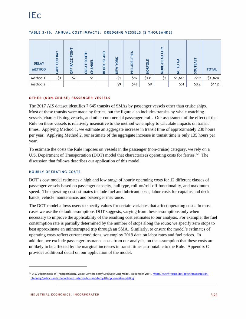
3-22

TABLE 3 -16. ANNUAL COST IMPACTS: DREDGING VESSELS ($ THOUSANDS)

DELAY

METHOD

CA

PE C

OD

BA

Y

OFF R

AC

E P

OIN

T

GR

EA

T S

OU

TH

CH

AN

NEL

BLO

CK

ISLA

ND

NEW

YO

RK

PH

ILA

DELPH

IA

NO

RFO

LK

MO

RE-H

EA

D C

ITY

NC

TO

GA

SO

UT

EA

ST

TOTAL

Method 1 -$1 $2 $1 -$1 $89 $131 $5 $1,616 -$19 $1,824

Method 2 $9 $43 $9 $51 $0.2 $112

OTHER (NON-CRUISE) PASSENGER VESSELS

The 2017 AIS dataset identifies 7,645 transits of SMAs by passenger vessels other than cruise ships.

Most of these transits were made by ferries, but the figure also includes transits by whale watching

vessels, charter fishing vessels, and other commercial passenger craft. Our assessment of the effect of the

Rule on these vessels is relatively insensitive to the method we employ to calculate impacts on transit

times. Applying Method 1, we estimate an aggregate increase in transit time of approximately 230 hours

per year. Applying Method 2, our estimate of the aggregate increase in transit time is only 135 hours per

year.

To estimate the costs the Rule imposes on vessels in the passenger (non-cruise) category, we rely on a

U.S. Department of Transportation (DOT) model that characterizes operating costs for ferries. 56 The

discussion that follows describes our application of this model.


DOT’s cost model estimates a high and low range of hourly operating costs for 12 different classes of

passenger vessels based on passenger capacity, hull type, roll-on/roll-off functionality, and maximum

speed. The operating cost estimates include fuel and lubricant costs, labor costs for captains and deck

hands, vehicle maintenance, and passenger insurance.

The DOT model allows users to specify values for certain variables that affect operating costs. In most

cases we use the default assumptions DOT suggests, varying from these assumptions only when

necessary to improve the applicability of the resulting cost estimates to our analysis. For example, the fuel

consumption rate is partially determined by the number of stops along the route; we specify zero stops to

best approximate an uninterrupted trip through an SMA. Similarly, to ensure the model’s estimates of

operating costs reflect current conditions, we employ 2019 data on labor rates and fuel prices. In

addition, we exclude passenger insurance costs from our analysis, on the assumption that these costs are

unlikely to be affected by the marginal increases in transit times attributable to the Rule. Appendix C

provides additional detail on our application of the model.

56 U.S. Department of Transportation, Volpe Center: Ferry Lifecycle Cost Model. December 2011. https://www.volpe.dot.gov/transportation-

planning/public-lands/department-interior-bus-and-ferry-lifecycle-cost-modeling.

https://www.volpe.dot.gov/transportation-planning/public-lands/department-interior-bus-and-ferry-lifecycle-cost-modeling


3-23

DOT’s model generates estimates of hourly operating costs for 12 types of vessels (see Appendix C). For

purposes of our analysis we calculate a weighted average operating cost, based on the distribution of

vessels represented in the 2017 AIS dataset and information on vessel characteristics obtained from the

National Census of Ferry Operators (NCFO).57 This calculation yields a weighted-average operating cost

of approximately $484 per hour.

ANNUAL COST IMPACTS

To assess the annual economic impact of the Rule on passenger (non-cruise) vessels, we multiply the

hourly cost figure cited above by the estimated impact of the Rule on transit times. Table 3-17 presents

our findings. As the table shows, we estimate that the Rule increases operating costs for passenger (non-

cruise) vessels by approximately $65 thousand to $112 thousand per year, depending on the method

employed to estimate the impact of the Rule on vessel transit times.

TABLE 3 -17. ANNUAL COST IMPACTS: OTHER (NON-CRUISE) PASSENGER VESSELS ($ THOUSANDS)

DELAY

METHOD

CA

PE C

OD

BA

Y

OFF R

AC

E P

OIN

T

GR

EA

T S

OU

TH

CH

AN

NEL

BLO

CK

ISLA

ND

NEW

YO

RK

PH

ILA

DELPH

IA

NO

RFO

LK

MO

RE-H

EA

D C

ITY

NC

TO

GA

SO

UT

EA

ST

TOTAL

Method 1 $33 $9 $4 $5 $2 -$3 -$1 $56 $6 $112

Method 2 $33 $9 $3 $2 $2 -$3 -$0.1 $18 $1 $65

LIMITATIONS

The analysis presented above does not consider the potential impact of the Rule on the seasonal operation

of high-speed ferries. The imposition of speed restrictions within an SMA may lead the operators of

high-speed ferries that transit SMAs to curtail service when the speed restrictions are in effect. This could

have an adverse effect on the profitability of such operations.58

A review of the ferry routes identified in the NCFO suggests that speed restrictions within SMAs likely

affect two high-speed ferry operators in Massachusetts: Bay State Cruise Company and Boston Harbor

Cruises. The Cape Cod Bay SMA’s restricted period ends May 15th; both companies resume the seasonal

operation of high-speed ferries from Boston to Provincetown on May 16th. NCFO records from years

prior to the Rule indicate that at that time, the seasonal operation of high-speed ferries from Boston to

Provincetown began May 1st. It is likely that the Rule directly affected the change in operating schedules.

57 The NCFO is a national survey of ferry owners and operators conducted every 2-4 years by the United States Bureau of Transportation Statistics.

Data are self-reported by ferry operators, and report characteristics of ferry operators and the vessels in their fleets, as well as ferry routes and

the terminals serviced by them. The most recent census was conducted in 2016.

58 Fast ferries typically operate at speeds in excess of 30 knots. Fast ferry operators’ business relies on the ability to travel at these high speeds to

deliver passengers between ports as efficiently as possible.

3-24

Whether the Rule has in fact had an adverse impact on the profitability of high-speed ferry operators is

unclear. Evaluating this impact would require estimates of the increase in annual revenue that might be

realized if the ferries were able to operate in the first half of May, as well as information on the associated

increase in operating costs. In the absence of reliable data on the effect of an expanded operating

schedule on annual ridership, we have not attempted to develop such estimates. We note, however, the

possibility of an adverse impact on profits and the relevance of such impacts in characterizing the costs of

the Rule.

PLEASURE CRAFT

Vessels classified in the AIS data as pleasure craft consist primarily of motorized, personal recreational

vessels. Pleasure craft subject to the Rule (i.e., those greater than 65 feet in length) consist primarily of

motor yachts (i.e., large motorboats) or large recreational fishing boats. Due to inconsistencies in the AIS

data, some sailing vessels equipped with auxiliary engines may also be included in the “pleasure vessel”

category.

The 2017 AIS dataset identifies approximately 6,600 transits of SMAs by pleasure craft. Our assessment

of the effect of the Rule on these vessels is relatively insensitive to the method we employ to calculate

impacts on transit times. Applying Method 1, we estimate an aggregate increase in transit time of

approximately 610 hours per year. Applying Method 2, our estimate of the aggregate increase in transit

time is approximately 440 hours per year.

Given that pleasure craft are designed primarily for recreational use, we have not attempted to quantify a

cost associated with the delays we estimate for these vessels. Their operators or passengers may

experience a loss in economic welfare if the vessel speed restrictions reduce their enjoyment of their time

on the water or delay them from reaching their destination as rapidly as they would otherwise. For others,

the vessel speed restrictions may have no effect on the quality of their recreational experience, and thus

no effect on economic welfare. Analysis of these impacts would require primary research, such as a

stated preference survey designed to quantify recreational boaters’ willingness to pay to operate at speeds

above 10 knots within each SMA during the restricted period. In the absence of such research we simply

note that vessel speed restrictions could adversely affect the quality of the recreational experience for

some boaters. The effect of such impacts on economic welfare, however, is unclear.

OTHER VESSELS

As noted in Chapter 2, approximately 6,600 transits included in the 2017 AIS dataset were made by

vessels in the “Other/Undetermined” vessel category. This category includes vessels that reported

multiple, conflicting vessel types in their AIS signals as well as vessels in categories with too few transits

to warrant independent analysis (e.g., pollution control vessels, pilot vessels, or port tenders and offshore

work vessels).


We estimate the impacts of the Rule on vessels in the “Other/Undetermined” category by using a

weighted average hourly cost figure for dredging, fishing, passenger (other), and towing/pushing vessels,

based on the distribution of transits in the AIS dataset. We exclude estimates of operating costs for

3-25

commercial shipping vessels and cruise ships from the calculation of the weighted average because the

availability of IHS data on these types of vessels makes it unlikely that any are included in the

“Other/Undetermined” category. As Table 3-18 illustrates, our calculation yields a weighted average

hourly operating cost estimate of approximately $589.

TABLE 3 -18. CALCULATION OF HOURLY OPERATING COST FOR OTHER/UNDETERMINED VESSELS

VESSEL TYPE

PERCENT OF

TRANSITS

AVERAGE HOURLY

OPERATING COST

WEIGHTED AVERAGE

HOURLY OPERATING COST

Dredging 3.8% $1,695.00 $65.17

Fishing 50.5% $231.18 $116.70

Passenger (Other) 15.5% $484.45 $75.26

Towing/Pushing 30.1% $1,101.00 $331.83

Total 100% $588.97

ANNUAL COST IMPACTS

To assess the annual economic impact of the Rule on vessels in the “Other/Undetermined” category, we

multiply the hourly cost figure cited above by the estimated impact of the Rule on the transits of these

vessels. Table 3-19 presents our findings. As the table shows, we estimate that the Rule increases

operating costs for vessels in the “Other/Undetermined” category by approximately $314 thousand to $1.5

million per year, depending on the method employed to estimate the impact of the Rule on vessel transit

times.

TABLE 3 -19. ANNUAL COST IMPACTS: OTHER/UNDETERMINED VESSELS ($ THOUSANDS)

DELAY

METHOD

CA

PE C

OD

BA

Y

OFF R

AC

E P

OIN

T

GR

EA

T S

OU

TH

CH

AN

NEL

BLO

CK

ISLA

ND

NEW

YO

RK

PH

ILA

DELPH

IA

NO

RFO

LK

MO

RE-H

EA

D C

ITY

NC

TO

GA

SO

UT

EA

ST

TOTAL

Method 1 $50 $111 -$27 $134 $997 $31 $46 $103 $31 $58 $1,535

Method 2 $50 $89 $1 -$0.5 $129 $6 $15 $31 -$8 $2 $314

SUMMARY

Table 3-20 summarizes our estimates of the Rule’s impact on annual operating costs. As the table

indicates, we estimate an annual impact of $28.3 million to $39.4 million, depending on the method

employed to estimate the impact of the Rule on transit times. Most of these costs are attributable to

impacts on container ships, and more generally to vessels operated by the commercial shipping industry

(bulk carriers, container ships, ro-ro vessels, tankers, and general cargo ships).

3-26

TABLE 3 -20. SUMMARY OF ANNUAL COST IMPACTS ($ THOUSANDS)

VESSEL TYPE DELAY METHOD 1 DELAY METHOD 2

Bulk Carrier $619 $346

Container $22,953 $20,025

Ro-Ro $3,381 $2,825

Tanker $1,693 $1,110

General Cargo $578 $461

Passenger (Cruise) $2,759 $2,677

Fishing $1,318 $147

Towing/Pushing $2,619 $244

Dredging $1,824 $112

Passenger (Other) $112 $65

Pleasure $0 $0

Other/Undetermined $1,535 $314

Total $39,391 $28,327

4-1

CHAPTER 4 | CONSIDERATION OF BROADER ECONOMIC IMPACTS

INTRODUCTION

Previous analyses have noted the possibility that the costs associated with the Rule could lead to changes

in the overall level or distribution of shipping activity along the Atlantic coast. These concerns were

likely heightened by economic conditions at the time the Rule was promulgated. At that time, the U.S.

was experiencing a significant recession, which began in December 2007 and continued until June 2009.59

When the Rule was promulgated in 2008, the effects of the recession were still unfolding.

An in-depth investigation of the potential impacts of the Rule on the level or distribution of economic

activity at U.S. ports would require a detailed analysis that is beyond the scope of this report.

Nonetheless, we can provide some insights on this issue by presenting a limited review of data on

shipping activity since implementation of the Rule. The discussion that follows summarizes our findings.

PORT CALLS

As a measure of potential impacts on the general level of economic activity at U.S. ports along the

Atlantic seaboard, we first assess the number of port calls reported in the period before and after the Rule.

To conduct this analysis, we rely upon data provided by the U.S. Maritime Administration (MARAD),

which reports the number of port calls by privately-owned, oceangoing merchant vessels of greater than

10,000 deadweight tons from 2002 to 2015.60 The MARAD data include port calls by oil, liquefied

natural gas (LNG), liquefied petroleum gas (LPG), and chemical tankers; container ships; dry bulk

carriers; ro-ro vessels; and other general cargo vessels. MARAD defines “calls” as the number of times a

vessel arrived at a port, facility, or terminal. The number of calls may include berth shifts, movements to

and from anchorage, or other activities related to vessel, port, or terminal operations.

Figure 4-1 presents the number of port calls by East Coast port from 2002 to 2015. Figure 4-2 presents

the aggregate number of port calls at these ports over the same period (excluding ports with fewer than

200 port calls in each year). We observe that the number of vessels entering ports on the East Coast has

remained relatively constant over time, both by port and in aggregate.

59 US Business Cycle Expansions and Contractions, National Bureau of Economic Research, accessed at https://www.nber.org/cycles/.

60 “Vessel Calls in U.S. Ports, Selected Terminals and Lightering Areas (2015).” U.S. Maritime Administration. Accessed at

https://www.maritime.dot.gov/data-reports/data-statistics/data-statistics.

https://www.nber.org/cycles/

https://www.maritime.dot.gov/data-reports/data-statistics/data-statistics

4-2

FIGURE 4-1. PORT CALLS AT EAST COAST PORTS, 2002 -2015

FIGURE 4-2. TOTAL PORT CALLS AT EAST COAST PORTS, 2002 -2015

4-3

IMPORT/EXPORT VALUES

As an additional indicator of shipping activity, we examine the value of goods traveling through East

Coast ports, either as imports into the U.S. or as exports out of the U.S. For this analysis, we rely upon

port-level import and export data from the U.S. Census Bureau’s Economic Indicators Division.61 We

reviewed monthly import and export data from 2003 to September 2019, compiled from electronic

records related to goods entering or leaving the U.S. The value of imports is based on the appraised value,

as estimated by U.S. Customs and Border Protection, while the value of exports is based on the “free

alongside ship” price – i.e., the value of exports at the U.S. port of export, based on transaction prices,

inland freight prices, and other charges in placing merchandise alongside the carrier at the port of

exportation.62

As shown in Figure 4-3, Figure 4-4, and Figure 4-5, the value of imports and exports from January 2003

to September 2019 decreased noticeably during the recession, but does not appear to have been adversely

affected in the long term, either for a particular port or in aggregate.

FIGURE 4-3. VALUE OF IMPORTS BY PORT, 2003 -2019

61 “U.S. Import and Export Merchandise Trade Statistics.” U.S. Census Bureau: Economic Indicators Division. Accessed at

https://usatrade.census.gov/data/Perspective60/Browse/BrowseTables.aspx.

62 “Guide to Foreign Trade Statistics.” U.S. Census Bureau. Accessed at https://www.census.gov/foreign-trade/guide/sec2.html.

https://usatrade.census.gov/data/Perspective60/Browse/BrowseTables.aspx

https://www.census.gov/foreign-trade/guide/sec2.html

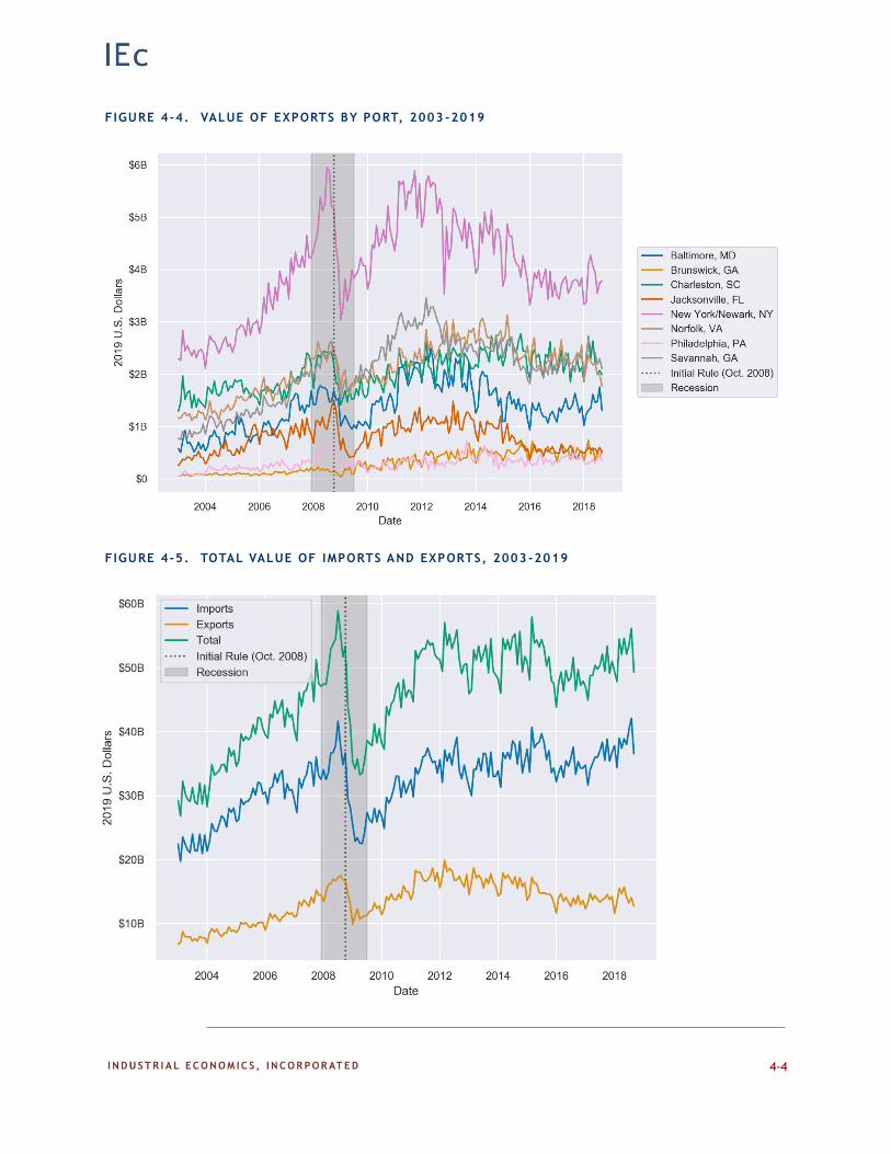
4-4

FIGURE 4-4. VALUE OF EXPORTS BY PORT, 2003 -2019

FIGURE 4-5. TOTAL VALUE OF IMPORTS AND EXPORTS, 2003 -2019

4-5

SUMMARY

Shipping activity at U.S. ports is influenced by many factors, including global economic conditions.

Given these considerations, a cursory review of the type presented here is insufficient to support

definitive conclusions concerning the potential impacts of the Rule on shipping activity. Nonetheless,

this review provides no prima facie evidence that the promulgation of the Rule has led to substantial

impacts on shipping activity. Overall, the value of goods entering and leaving East Coast ports recovered

following the recession and has remained relatively constant over the past decade. Similarly, the number

of vessels entering ports on the East Coast has remained relatively constant over time, both by port and in

aggregate. Thus, a high-level review of the data suggests the Rule has not had a readily observable effect

on the volume or value of economic activity at potentially affected ports.

5-1

CHAPTER 5 | CONCLUSIONS

PRINCIPAL FINDINGS

The analysis presented in this report estimates the direct costs attributable to the Final Rule to Implement

Speed Restrictions to Reduce the Threat of Ship Collisions with North Atlantic Right Whales. The

analysis is based on AIS data that allow us to estimate the speed with which vessels that are subject to the

Rule transit the Seasonal Management Areas where the vessel speed restrictions apply. We estimate the

impact of the Rule on transit times for various types of vessels by comparing vessel operations during

restricted periods – i.e., the seasonal periods when the speed restrictions are in effect – to counterfactual

scenarios that are based on the speeds at which vessels operate when the speed restrictions are not in

effect. We calculate the cost of the estimated increase in transit times by applying estimates of hourly

operating costs for each type of vessel.

Depending on the method employed to characterize the Rule’s impact on transit times, we estimate its

direct costs at approximately $28.3 million to $39.4 million annually. The analysis indicates that the cost

to commercial shipping operations alone ranges from $24.8 million to $29.2 million per year. Most of

these costs are associated with the operation of container ships, reflecting the large number of container

ship transits that are affected by the Rule, the magnitude of the delays imposed by the vessel speed

restrictions, and the high hourly cost of operating these types of vessels.

LIMITATIONS AND UNCERTAINTIES

Our analysis is subject to number of limitations and uncertainties. Notably, the AIS data we use to

estimate the impact of the Rule on SMA transits are subject to a number of data quality concerns,

including records that report questionable average speeds, distances traveled, or elapsed operating times,

as well as records that are unsuitable for our specific analytic needs (e.g., transits which appear to have

“clipped” the bounds of an SMA rather than traveled through it for a significant length of time).

Additionally, the vessel type and length designations reported in AIS records are often ambiguous,

complicating the classification of transits by vessel type and perhaps leading us to include in the analysis

transits made by vessels that are not subject to the Rule.63

Another important limitation of our analysis is that our methods treat observed differences in transit

speeds during an SMA’s restricted and unrestricted periods as entirely attributable to the Rule. It is quite

possible – and in fact likely – that at least some of the observed differences are due to other factors, such

as seasonal differences in weather and sea conditions, seasonal fluctuations in the activity of commercial

63 As explained in Chapter 2, Data Sources, AIS Data, when the vessel length is ambiguous, we err on the side of over-including vessels in our

analysis by using the maximum length reported in the vessel’s AIS signal.

5-2

fishing fleets, seasonal variation in the use of pleasure craft, or other factors. Failure to control for these

factors may bias our assessment of the Rule’s costs. The potential magnitude and direction of any such

bias, however, is unknown.

Our estimates of vessel operating costs are also subject to considerable uncertainty. In the absence of

reliable data on vessel capital costs, we limit our analysis of the Rule’s effects on the commercial

shipping sector to impacts on variable and quasi-fixed/variable costs. For consistency – when available

data permit – we follow a similar approach in other sectors. As discussed in greater detail in Chapter 3,

this approach is appropriate if the Rule has no impact on capital costs; i.e., if marginal changes in

operating speeds do not lead to additional demand for shipping capacity or for vessels of a specific type

(e.g., dredging or fishing vessels). If this is not the case, failure to account for the need for additional

vessel capacity will lead us to underestimate the costs attributable to the Rule.

In addition to the caveats noted above, it is important to emphasize that we lack data on hourly operating

costs for several types of vessels (e.g., cruise ships, towing/pushing vessels, dredging vessels). In the

interest of providing an estimate of the Rule’s costs that is as complete as possible, we have relied on

other types of data (e.g., hourly rate information) to characterize hourly operating costs. The resulting

estimates are subject to substantial uncertainty and should be considered only rough approximations of

actual costs.

POTENTIAL REFINEMENTS AND ADDITIONAL APPLICATIONS

The analysis presented in this report is based entirely on AIS data and estimates of vessel operating costs

derived from secondary sources. Direct outreach to the commercial shipping industry or to

representatives of the other sectors the Rule affects would offer an opportunity to ground truth our

findings and develop a clearer understanding of the Rule’s impact on vessel operations. It might also

provide an opportunity to refine our estimates of vessel operating costs.

In addition to improving our understanding of the Rule’s current impacts, the data and methods employed

in this report could be applied to evaluate modifications to the Rule designed to improve its cost-

effectiveness or provide additional protections to right whales. These modifications might include, for

example:

• Designating new SMAs;

• Changing the spatial or temporal extent of established SMAs;

• Revising the Rule’s specification of vessels that are subject to speed restrictions;

• Changing the maximum permissible speed within SMAs; or

• Establishing mandatory limits on vessel speed within DMAs.

Should NMFS wish to consider potential revisions to the Rule, we could expand our analysis to evaluate

any of these alternatives.

A-1

APPENDIX A | ADDITIONAL STATISTICS ON SMA TRANSITS

A-2

TABLE A-1. TRANSITS BY VESSEL TYPE, SMA, AND PERIOD

VESSEL TYPE

CAPE COD BAY OFF RACE POINT

GREAT SOUTH

CHANNEL BLOCK ISLAND NEW YORK

RESTR. UNRESTR. RESTR. UNRESTR. RESTR. UNRESTR. RESTR. UNRESTR. RESTR. UNRESTR.

Bulk Carrier 1 20 121 36 142 122 125 192 221

Container 55 326 140 257 3 1 1,976 1,929

Ro-Ro 17 30 18 94 35 73 178 201 515 543

Tanker 14 35 44 224 139 238 146 183 1,139 1,318

General Cargo 1 7 19 19 34 64 60 117 97

Passenger (Cruise) 3 52 2 174 57 129 3 76 172 411

Fishing 545 383 599 1,529 2,230 3,793 2,560 3,828 290 755

Towing/Pushing 596 968 32 219 7 15 281 311 1,659 1,394

Dredging 3 5 2 4 1 1 4 40 72

Passenger (Other) 60 2,490 35 1,493 2 69 128 128 497

Pleasure 7 425 1 275 28 81 35 393 45 532

Other/Undetermined 102 739 75 421 42 206 417 716 375 723

Total 1,347 5,129 890 4,899 2,734 4,971 3,882 6,022 6,648 8,492

A-3

VESSEL TYPE

PHILADELPHIA NORFOLK MOREHEAD CITY

NORTH CAROLINA

TO GEORGIA SOUTHEAST

TOTAL RESTR. UNRESTR. RESTR. UNRESTR. RESTR. UNRESTR. RESTR. UNRESTR. RESTR. UNRESTR.

Bulk Carrier 223 233 942 903 28 27 351 400 130 198 4,415

Container 628 647 1,701 1,743 1 3,426 3,570 433 593 17,429

Ro-Ro 188 194 642 700 405 448 842 1,144 6,267

Tanker 620 724 168 173 27 35 432 448 142 179 6,428

General Cargo 325 234 236 271 74 74 370 336 210 280 2,828

Passenger (Cruise) 2 8 76 163 8 7 130 111 103 93 1,780

Fishing 1,310 1,568 813 1,543 611 366 396 741 388 592 24,840

Towing/Pushing 1,505 1,309 530 668 173 137 1,872 1,012 789 1,354 14,831

Dredging 107 26 94 325 10 9 640 61 415 73 1,892

Passenger (Other) 43 821 98 450 6 34 430 462 160 239 7,645

Pleasure 49 585 69 515 163 628 510 1,342 198 703 6,584

Other/Undetermined 123 308 219 393 109 174 519 381 245 321 6,608

Total 5,123 6,657 5,588 7,847 1,209 1,492 9,481 9,312 4,055 5,769 101,547

A-4

TABLE A-2. MEAN VESSEL SPEED (KNOTS) BY VESSEL TYPE, SMA, AND PERIOD

VESSEL TYPE

CAPE COD BAY OFF RACE POINT

GREAT SOUTH

CHANNEL BLOCK ISLAND NEW YORK


Bulk Carrier 13.0 10.9 11.0 11.0 11.1 10.8 11.6 9.2 10.2

Container 9.8 13.9 9.5 14.2 11.9 11.8 9.1 12.6

Ro-Ro 7.3 8.8 8.4 13.3 9.1 14.0 8.9 13.5 9.2 12.0

Tanker 9.7 11.0 9.6 11.8 10.0 11.9 10.4 12.4 9.2 10.5

General Cargo 8.6 9.6 12.8 11.3 12.5 10.5 11.9 9.7 11.5

Passenger (Cruise) 9.3 12.0 12.6 15.1 10.8 14.5 9.7 14.4 10.3 14.5

Fishing 7.2 7.8 5.6 6.8 6.3 5.8 7.7 7.8 8.9 8.2

Towing/Pushing 8.3 8.6 8.8 9.4 9.3 14.2 9.0 9.2 7.8 8.3

Dredging 7.2 7.0 6.8 8.6 8.4 8.8 8.9 5.5 6.9

Passenger (Other) 12.2 23.3 8.4 21.1 17.2 11.6 11.8 14.6 14.5

Pleasure 15.8 13.4 31.3 13.0 11.0 10.2 10.1 15.3 15.7 16.2

Other/Undetermined 8.4 15.8 5.1 13.4 6.8 5.8 12.0 10.9 10.1 11.9

A-5

VESSEL TYPE

PHILADELPHIA NORFOLK MOREHEAD CITY

NORTH CAROLINA

TO GEORGIA SOUTHEAST


Bulk Carrier 9.5 11.0 9.7 10.5 9.5 10.8 10.2 10.9 9.2 10.9

Container 9.1 13.1 9.0 13.1 13.1 10.9 13.0 9.5 13.8

Ro-Ro 9.0 13.0 9.2 13.7 11.0 13.6 9.6 12.9

Tanker 9.2 10.9 9.7 11.8 9.2 10.1 10.2 11.8 9.4 12.0

General Cargo 9.2 12.6 9.7 12.2 9.4 11.1 10.5 11.5 9.6 11.9

Passenger (Cruise) 10.5 11.3 10.1 15.4 9.6 12.1 11.6 13.6 9.7 12.6

Fishing 7.7 8.1 8.7 10.2 7.2 10.2 7.4 10.1 5.2 5.1

Towing/Pushing 7.4 7.6 7.9 7.7 6.8 6.8 7.1 7.7 7.9 7.8

Dredging 7.6 8.1 8.3 9.7 7.2 7.0 5.8 7.1 6.5 6.1

Passenger (Other) 11.8 12.7 11.2 10.5 23.4 16.4 8.6 9.1 8.8 9.1

Pleasure 16.4 18.5 17.2 17.1 18.4 18.9 16.0 17.3 15.2 17.0

Other/Undetermined 7.9 8.8 10.2 10.4 9.1 13.2 10.7 9.0 9.1 9.2

A-6

FIGURE A-1. DISTRIBUTION OF CONTAINER VESSEL SPEEDS (KNOTS) BY SMA AND PERIOD

FIGURE A-2. DISTRIBUTION OF TANKER VESSEL SPEEDS (KNOTS) BY SMA AND PERIOD

A-7

FIGURE A-3. DISTRIBUTION OF RO-RO VESSEL SPEEDS (KNOTS) BY SMA AND PERIOD

FIGURE A-4. DISTRIBUTION OF BULK CARRIER VESSEL SPEEDS (KNOTS) BY SMA AND PERIOD

A-8

FIGURE A-5. DISTRIBUTION OF GENERAL CARGO VESSEL SPEEDS (KNOTS) BY SMA AND PERIOD

FIGURE A-6. DISTRIBUTION OF FISHING VESSEL SPEEDS (KNOTS) BY SMA AND PERIOD

A-9

FIGURE A-7. DISTRIBUTION OF TOWING/PUSHING VESSEL SPEEDS (KNOTS) BY SMA AND PERIOD

FIGURE A-8. DISTRIBUTION OF CRUISE PASSENGER VESS EL SPEEDS (KNOTS) BY SMA AND PERIOD

A-10

FIGURE A-9. DISTRIBUTION OF OTHER PASSENGER VESSEL SPEEDS (KNOTS) BY SMA AND PERIOD

FIGURE A-10. DISTRIBUTION OF PLEASURE VESSEL SPEEDS (KNOTS) BY SMA AND PERIOD

A-11

FIGURE A-11. DISTRIBUTION OF DREDGING VESSEL SPEEDS (KNOTS) BY SMA AND PERIOD

FIGURE A-12. DISTRIBUTION OF OTHER / UNDETERMINED VESSEL SPEEDS (KNOTS ) BY SMA AND

PERIOD

B-1

APPENDIX B | IMPACTS ASSUMING FULL COMPLIANCE

INTRODUCTION

An important consideration in evaluating the effect of the Rule is the treatment of non-compliant transits.

The main body of this report characterizes the effects of the Rule as implemented, including transits of

SMAs that violate the Rule. This approach is appropriate for a retrospective analysis. At the same time,

it is important to consider what the impact of the Rule would be if full compliance were achieved. This

appendix presents an analysis that assumes full compliance. It employs methods identical to those

described in the main body of the report, with one modification: average operating speeds during the

restricted period are calculated after setting all transits that occurred at non-compliant speeds to the

maximum compliant speed – 10 knots. 64 Mathematically, this methodology may be written as:

𝑑𝑒𝑙𝑎𝑦 = 𝑡𝑖𝑚𝑒𝑜𝑏𝑠𝑒𝑟𝑣𝑒𝑑∗ − 𝑡𝑖𝑚𝑒𝑐𝑓 =


𝑠𝑝𝑒𝑒𝑑𝑜𝑏𝑠𝑒𝑟𝑣𝑒𝑑∗ −


𝑠𝑝𝑒𝑒𝑑𝑐𝑓

where

𝑠𝑝𝑒𝑒𝑑𝑜𝑏𝑠𝑒𝑟𝑣𝑒𝑑∗ = {

𝑠𝑝𝑒𝑒𝑑𝑜𝑏𝑠𝑒𝑟𝑣𝑒𝑑 𝑖𝑓 𝑠𝑝𝑒𝑒𝑑𝑜𝑏𝑠𝑒𝑟𝑣𝑒𝑑 ≤ 1010 𝑖𝑓 𝑠𝑝𝑒𝑒𝑑𝑜𝑏𝑠𝑒𝑟𝑣𝑒𝑑 > 10

This adjustment provides some perspective on the implications of full compliance for various types of

vessels, particularly those that show relatively high rates of non-compliance. We refer to the methods that

employ this adjustment as Method 1A and Method 2A.

METHOD 1A: COMPARISON OF MEANS WITH ASSUMPTION OF FULL COMPLIANCE

Under Method 1A, as was the case under Method 1, we assume that each transit in the restricted period

would have – but for the Rule – occurred at the average speed in the unrestricted period. To reflect the

impact of full compliance, however, we modify observed transit speeds during the restricted period as

described above. This modification increases the estimated impact of the rule on transit times.

Figure B-1 illustrates the impact of the assumption of full compliance on the analysis, focusing on the

same set of transits presented in Figure 2-4. Under Method 1A, we modify the distribution of restricted-

period transits, resetting the speed of all transits that occurred at non-compliant speeds to 10 knots. This

modification reduces the average speed of restricted-period transits (albeit only slightly in this case, as

most transits occurred at less than 10 knots). There is no difference in the counterfactual speed employed

in the analysis, which remains at approximately 12 knots. Thus, the assumption of full compliance

64 For example, if a restricted-period transit of 18 nautical miles occurred at an average speed of 14 knots, taking an estimated 1.29 hours, we

assume that this transit would have occurred at 10 knots, taking an estimated 1.8 hours.

B-2

increases the estimated impact of the Rule on transit times. Table B-1 presents the total estimated delay

under Method 1A by vessel type and SMA. Table B-2 presents our estimate of the associated costs.

FIGURE B-1. TANKER VESSELS, NORFOLK SMA (NOVEMBER 1 – APRIL 30): FULL COMPLIANCE

SCENARIO

Notes: y-axis truncated to preserve readability of graph;

restricted-period histogram bins change slightly even for unaffected transits.

B-3

TABLE B-1. TOTAL DELAY (HOURS) BY VESSEL TYPE AND SMA, METHOD 1A

VESSEL TYPE C

APE C

OD

BA

Y

OFF R

AC

E P

OIN

T

GR

EA

T S

OU

TH

CH

AN

NEL

BLO

CK

ISLA

ND

NEW

YO

RK

PH

ILA

DELPH

IA

NO

RFO

LK

MO

REH

EA

D C

ITY

NC

TO

GA

SO

UT

HEA

ST

TOTAL

Bulk Carrier 11 25 85 99 68 244 13 123 88 756

Container 92 280 1 1,538 370 1,280 2,156 467 6,184

Ro-Ro 14 28 64 237 362 119 474 292 809 2,399

Tanker 4 39 168 120 572 208 87 10 214 115 1,536

General Cargo 5 22 46 65 166 120 34 143 153 754

Passenger (Cruise)

2 3 94 3 159 0.4 58 6 136 82 543

Fishing 161 1,238 -97 470 29 185 407 1,253 2,643 652 6,942

Towing / Pushing

206 11 11 56 432 265 69 48 1,183 185 2,466

Dredging -0.5 1 0.3 -1 54 79 3 957 -10 1,083

Passenger (Other)

93 19 21 62 11 8 4 156 30 403

Pleasure 4 1 12 30 35 46 56 163 1,113 360 1,820

Other / Undetermined

88 188 -45 274 1,770 59 112 191 211 128 2,976

Total 572 1,635 533 1,342 5,122 1,553 2,995 1,724 9,327 3,060 27,861

B-4

TABLE B-2. TOTAL COSTS BY VESSEL TYPE AND SMA, METHOD 1A ($ THOUSANDS)

VESSEL TYPE

CA

PE C

OD

BA

Y

OFF R

AC

E P

OIN

T

GR

EA

T S

OU

TH

CH

AN

NEL

BLO

CK

ISLA

ND

NEW

YO

RK

PH

ILA

DELPH

IA

NO

RFO

LK

MO

REH

EA

D C

ITY

NC

TO

GA

SO

UT

EA

ST

TOTAL

Bulk Carrier $11 $24 $84 $104 $70 $306 $11 $119 $94 $823

Container $459 $1,497 $3 $6,686 $916 $5,979 $9,648 $1,574 $26,762

Ro-Ro $13 $33 $91 $339 $559 $176 $748 $475 $1,186 $3,621

Tanker $5 $62 $231 $133 $731 $300 $90 $10 $226 $151 $1,940

General Cargo $4 $20 $39 $53 $179 $109 $31 $125 $136 $695

Passenger (Cruise)

$14 $16 $565 $16 $959 $2 $348 $37 $817 $497 $3,272

Fishing $35 $324 -$87 $119 $6 $34 $79 $211 $512 $130 $1,364

Towing / Pushing

$227 $12 $12 $62 $476 $292 $76 $53 $1,303 $204 $2,715

Dredging -$1 $2 $1 -$1 $91 $135 $5 $1,621 -$17 $1,835

Passenger (Other)

$45 $9 $10 $30 $5 $4 $2 $76 $14 $195

Pleasure


$52 $111 -$27 $161 $1,042 $35 $66 $112 $124 $75 $1,753

Total $389 $1,044 $2,327 $966 $10,645 $2,099 $7,940 $473 $15,047 $4,046 $44,975

B-5

METHOD 2A: COMPARISON OF HIGH -SPEED TRANSITS WITH ASSUMPTION OF FULL COMPLIANCE

Under Method 2A, as was the case under Method 2, we assume that – but for the Rule – the same

percentage of transits would have occurred at speeds of greater than 10 knots in both the restricted and

unrestricted periods, and that the average speed of these transits in the restricted period would be equal to

the average speed of the transits in the unrestricted period. To reflect the impact of full compliance,

however, we modify observed transit speeds during the restricted period as described above. This

modification increases the estimated impact of the rule on transit times. Table B-3 presents the total

estimated delay under Method 2A by vessel type and SMA. Table B-4 presents our estimate of the

associated costs.

TABLE B-3. TOTAL DELAY (HOURS) BY VESSEL TYPE AND SMA, METHOD 2A

VESSEL TYPE

CA

PE C

OD

BA

Y

OFF R

AC

E P

OIN

T

GR

EA

T S

OU

TH

CH

AN

NEL

BLO

CK

ISLA

ND

NEW

YO

RK

PH

ILA

DELPH

IA

NO

RFO

LK

MO

REH

EA

D C

ITY

NC

TO

GA

SO

UT

HEA

ST

TOTAL

Bulk Carrier 11 25 58 41 50 170 7 96 61 517

Container 83 250 0.3 1,273 301 1,105 2,009 415 5,435

Ro-Ro 4 26 55 182 272 100 428 269 680 2,015

Tanker 5 34 160 101 287 140 74 7 178 93 1,078

General Cargo 5 20 35 43 136 107 24 131 120 622

Passenger (Cruise)

2 3 91 3 159 0.4 57 3 127 84 529

Fishing 3 1 29 22 25 12 179 425 224 7 927

Towing / Pushing

21 2 0.2 23 47 24 12 1 156 22 309

Dredging 6 26 7 33 1 73

Passenger (Other)

92 18 17 56 10 9 3 78 19 303

Pleasure 3 1 22 22 32 43 53 145 1,018 304 1,644


87 152 2 42 296 17 59 69 135 32 892

Total 217 336 652 506 2,537 859 2,260 684 4,454 1,838 14,343

B-6

TABLE B-4. TOTAL COSTS BY VESSEL TYPE AND SMA, METHOD 2A ($ THOUSANDS)

VESSEL TYPE

CA

PE C

OD

BA

Y

OFF R

AC

E P

OIN

T

GR

EA

T S

OU

TH

CH

AN

NEL

BLO

CK

ISLA

ND

NEW

YO

RK

PH

ILA

DELPH

IA

NO

RFO

LK

MO

REH

EA

D C

ITY

NC

TO

GA

SO

UT

HEA

ST

TOTAL

Bulk Carrier $11 $23 $54 $42 $50 $210 $6 $93 $60 $550

Container $416 $1,338 $1 $5,604 $742 $5,235 $9,079 $1,420 $23,834

Ro-Ro $6 $33 $79 $263 $421 $147 $677 $435 $1,002 $3,064

Tanker $5 $53 $227 $114 $356 $198 $80 $7 $189 $128 $1,357

General Cargo $4 $17 $36 $33 $147 $98 $21 $117 $105 $577

Passenger (Cruise)

$12 $18 $547 $17 $957 $2 $345 $17 $767 $508 $3,191

Fishing $1 $0.2 $10 $8 $5 $2 $38 $78 $48 $2 $192

Towing / Pushing

$23 $2 $0.3 $25 $52 $26 $13 $1 $172 $24 $340

Dredging $9 $44 $12 $56 $1 $123

Passenger (Other)

$45 $9 $8 $27 $5 $4 $2 $38 $9 $147

Pleasure


$51 $90 $1 $25 $174 $10 $35 $41 $80 $19 $525

Total $144 $636 $2,242 $551 $7,682 $1,374 $6,747 $173 $11,073 $3,279 $33,901

SUMMARY

Table B-5 compares the results of the full-compliance analysis to the results of the analysis presented with

no adjustment for non-compliance. As the table indicates, the assumption of full compliance with the

Rule increases our estimate of the costs associated with the vessel speed restrictions by approximately

$5.6 million per year, regardless of whether we employ Method 1 or Method 2 to calculate the Rule’s

effect. Approximately 68 percent of this increase is attributable to the additional cost container ships

would incur to achieve full compliance. As the charts presented in Appendix A indicate, this finding is

not a result of a disproportionately high degree of non-compliance among container ships. Rather, it

reflects the relatively high hourly operating costs of these vessels, coupled with the large share of affected

transits that container ships represent.

B-7

TABLE B-5. ESTIMATED COSTS BY VESSEL TYPE AND METHOD ($ THOUSANDS)

VESSEL TYPE METHOD 1 METHOD 1A METHOD 2 METHOD 2A

Bulk Carrier $619 $823 $346 $550

Container $22,953 $26,762 $20,025 $23,834

Ro-Ro $3,381 $3,621 $2,825 $3,064

Tanker $1,693 $1,940 $1,110 $1,357

General Cargo $578 $695 $461 $577

Passenger (Cruise) $2,759 $3,272 $2,677 $3,191

Fishing $1,318 $1,364 $147 $192

Towing / Pushing $2,619 $2,715 $244 $340

Dredging $1,824 $1,835 $112 $123

Passenger (Other) $112 $195 $65 $147

Pleasure NA NA NA NA

Other / Undetermined $1,535 $1,753 $314 $525

Total $39,391 $44,975 $28,327 $33,901

C-1

APPENDIX C | NOTES ON ESTIMATES OF VESSEL OPERATING COSTS

FISHING VESSEL COSTS

Table C-1 summarizes the responses to the GMRI survey on alternative occupations for commercial

fishermen and illustrates the calculations used to estimate the implicit hourly value of fishermen’s time.

TABLE C-1. CALCULATION OF IMPLICIT VALUE OF FISHERMEN’S TIME

ALTERNATIVE

OCCUPATION

PERCENT OF

RESPONDENTS

THAT IDENTIFIED

ALTERNATIVE*

NORMALIZED

DISTRIBUTION

OF RESPONSES

AVERAGE

2018 BLS

WAGE RATE

BLS OCCUPATIONAL CATEGORIES

INCORPORATED INTO AVERAGE

WAGE RATE

Carpentry/Trades/ Mechanic

28% 41% $22.80 Carpenters; Automotive Service Technicians and Mechanics

Other Commercial Fishing/Merchant Marine/Boat Building and Maintenance

26% 38% $27.39

Fishers and Related Fishing Workers; Motorboat Mechanics; Sailors and Marine Oilers; Captains, Mates, and Pilots of Water Vessels

Other Business 8% 12% $36.98 Business and Financial Operations Occupations

Truck Driver/Equipment Operator

3% 4% $23.71

Heavy and Tractor-Trailer Truck Drivers; Operating Engineers and Other Construction Equipment Operators

Education 2% 3% $27.22 Education, Training, and Library Occupations

Police/Firefighter/ EMT/Military

1% 1% $25.06

Police and Sheriff's Patrol Officers; Firefighters; Emergency Medical Technicians and Paramedics

Engineering 1% 1% $44.62 Mechanical Engineers

Other 10% N/A

Retire 2% N/A

Don't Know 16% N/A

Weighted Average $26.69

Weighted Average (Inflated to 2019 Dollars)

$27.03

*Because the survey permitted multiple responses, these figures do not sum to 100 percent.

C-2

OTHER PASSENGER VESSEL COSTS

Table C-2 presents the inputs specified in applying DOT’s ferry cost model to obtain hourly operating

costs for passenger vessels other than cruise ships.

TABLE C-2. FERRY COST MODEL INPUTS

COST CATEGORY INPUT VALUE

Fuel/Lubricant

How many stops will there be? None

Service Speed/Max Speed 0.8

Stop Time (min) 5

Lubricant Cost/Gallon (2019 $) $8.00

Diesel Fuel Cost/Gallon (2019 $) $3.091

Wages

Captain Hourly Wage Rate (2019 $) $31.892

Deckhand Hourly Wage Rate (2019 $) $16.363

Labor Overhead Rate 15%

Notes:

1. Diesel price is taken from the average diesel price for East Coast ports in 2019. This figure was obtained from the

U.S. Energy Information Administration’s Petroleum price tool, accessed at:

https://www.eia.gov/dnav/pet/pet_pri_gnd_a_epd2d_pte_dpgal_a.htm.

2. Estimated using U.S. Bureau of Labor Statistics recorded median hourly rate for a captain, mate, or pilot of a water

vessel within NAICS code 483100 (Deep Sea, Coastal, and Great Lakes Water Transportation). Accessed at:

https://www.bls.gov/oes/current/naics4_483100.htm. Accessed October 3, 2019.

3. Estimated using U.S. Bureau of Labor Statistics recorded median hourly rate for a laborer/material mover within

NAICS code 483100 (Deep Sea, Coastal, and Great Lakes Water Transportation). Accessed at:


We assume no stops along the ferry route, so that the model best represents an uninterrupted transit

through an SMA.65 The model also adds hourly costs for insurance, which is calculated by dividing the

total estimated number of passengers serviced each year by the total estimated operating hours, then

multiplying the result by a fixed cost per passenger. We do not expect delays resulting from the Rule to

affect the number of passengers serviced in a year, so we exclude these insurance costs from the total

hourly cost calculation. Table C-3 presents the resulting cost estimates for each type of vessel specified in

the model.

65 When the number of stops is greater than zero, the estimated hourly operating costs are also affected by the user’s input regarding round trip

distance. As we assume zero stops, this parameter is not relevant to our analysis.

https://www.eia.gov/dnav/pet/pet_pri_gnd_a_epd2d_pte_dpgal_a.htm

https://www.bls.gov/oes/current/naics4_483100.htm

https://www.bls.gov/oes/current/naics4_483100.htm

C-3

TABLE C-3. PASSENGER VESSEL COST MODEL OUTPUTS BY VESSEL CLASS

PASSENGER

CAPACITY

MAXIMUM

SPEED (KNOTS)

ROLL-ON /

ROLL-OFF

VEHICLE

CAPACITY

HOURLY OPERATING COST (2019 $)

LOW HIGH AVERAGE

1-30 No $64.28 $84.68 $74.48

31-50 (pontoon) No $117.70 $136.13 $126.91

31-50 (monohull or catamaran)

No $116.93 $157.89 $137.41

51-100 <20 No $126.15 $156.03 $141.09

51-100 >20 No $153.66 $293.17 $223.41

101-150 <20 No $117.70 $304.32 $211.01

101-150 >20 No $239.81 $547.02 $393.41

151-300 No $292.79 $870.25 $581.52

<100 Yes <10 $105.02 $176.70 $140.86

<500 Yes <10 $214.32 $480.57 $347.44

<500 Yes <50 $189.10 $683.70 $436.40

250-500 Yes 45-100 $3,246.90 $3,515.79 $3,381.34

Source: United States Department of Transportation, Volpe Center. Department of the Interior - Bus and Ferry Lifecycle Cost Modeling. December 2011.

CRUISE SHIP OPERATING COSTS

This section provides details underlying the calculation of cruise ship operating costs presented in Chapter

3. We develop these estimates using SEC Form 10-K annual filings for three large cruise companies:

Carnival Corporation & PLC; Royal Caribbean Cruises Ltd.; and Norwegian Cruise Line Holdings.

As noted in Chapter 3, we estimate hourly cruise ship operating costs using the following equation:

𝑂𝑝𝑒𝑟𝑎𝑡𝑖𝑛𝑔 𝐶𝑜𝑠𝑡𝑠 𝑝𝑒𝑟 𝑉𝑒𝑠𝑠𝑒𝑙 𝑝𝑒𝑟 𝐷𝑎𝑦 =(

𝐹𝑙𝑒𝑒𝑡𝑤𝑖𝑑𝑒 𝐴𝑛𝑛𝑢𝑎𝑙 𝑂𝑝𝑒𝑟𝑎𝑡𝑖𝑛𝑔 𝐶𝑜𝑠𝑡𝑠𝑁𝑢𝑚𝑏𝑒𝑟 𝑜𝑓 𝑉𝑒𝑠𝑠𝑒𝑙𝑠

)

𝐴𝑛𝑛𝑢𝑎𝑙 𝑂𝑝𝑒𝑟𝑎𝑡𝑖𝑛𝑔 𝐷𝑎𝑦𝑠 𝑝𝑒𝑟 𝑉𝑒𝑠𝑠𝑒𝑙

We divide operating costs per vessel per day by 24 to estimate hourly operating costs per vessel. The

discussion below describes the steps taken to calculate the number of vessels in each company’s fleet and

the annual operating days of the average vessel in each fleet.

DETERMINING FLEET S IZE

The 10-K filings for Carnival, Royal Caribbean, and Norwegian disclose the number of vessels each

company operates. In tabulating the size of each fleet, we consider only those vessels whose operating

costs are captured in the 10-K filings. We exclude, for example, vessels operated under Royal

Caribbean’s Pullmantur brand, as Royal Caribbean owns only a 49 percent share of the brand, and

therefore is not required to include financial information for this cruise line in its Form 10-K filings. The

filings information does not disaggregate costs by region; therefore, our tabulation of the size of each fleet

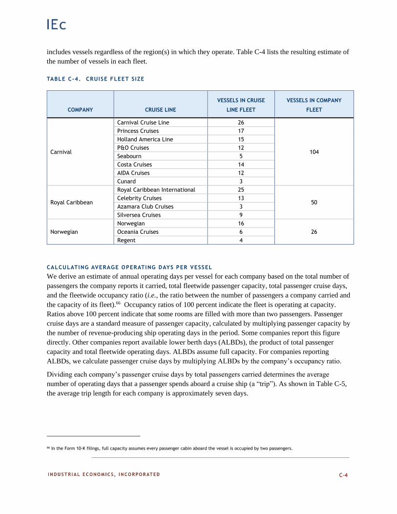
C-4

includes vessels regardless of the region(s) in which they operate. Table C-4 lists the resulting estimate of

the number of vessels in each fleet.

TABLE C-4. CRUISE FLEET SIZE

COMPANY CRUISE LINE

VESSELS IN CRUISE

LINE FLEET

VESSELS IN COMPANY

FLEET

Carnival

Carnival Cruise Line 26

104

Princess Cruises 17

Holland America Line 15

P&O Cruises 12

Seabourn 5

Costa Cruises 14

AIDA Cruises 12

Cunard 3

Royal Caribbean

Royal Caribbean International 25

50 Celebrity Cruises 13

Azamara Club Cruises 3

Silversea Cruises 9

Norwegian

Norwegian 16

26 Oceania Cruises 6

Regent 4

CALCULATING AVERAGE OPERATING DAYS PER VESSEL

We derive an estimate of annual operating days per vessel for each company based on the total number of

passengers the company reports it carried, total fleetwide passenger capacity, total passenger cruise days,

and the fleetwide occupancy ratio (i.e., the ratio between the number of passengers a company carried and

the capacity of its fleet).66 Occupancy ratios of 100 percent indicate the fleet is operating at capacity.

Ratios above 100 percent indicate that some rooms are filled with more than two passengers. Passenger

cruise days are a standard measure of passenger capacity, calculated by multiplying passenger capacity by

the number of revenue-producing ship operating days in the period. Some companies report this figure

directly. Other companies report available lower berth days (ALBDs), the product of total passenger

capacity and total fleetwide operating days. ALBDs assume full capacity. For companies reporting

ALBDs, we calculate passenger cruise days by multiplying ALBDs by the company’s occupancy ratio.

Dividing each company’s passenger cruise days by total passengers carried determines the average

number of operating days that a passenger spends aboard a cruise ship (a “trip”). As shown in Table C-5,

the average trip length for each company is approximately seven days.

66 In the Form 10-K filings, full capacity assumes every passenger cabin aboard the vessel is occupied by two passengers.

C-5

TABLE C-5. AVERAGE CRUISE TRIP LENGTH

COMPANY PASSENGER CRUISE DAYS PASSENGERS CARRIED

AVERAGE TRIP LENGTH

(DAYS)

Carnival 89,659,168 12,407,000 7.23

Royal Caribbean 41,853,052 6,078,201 6.89

Norwegian 20,276,568 2,795,101 7.25

We calculate the number of trips the average vessel takes per year by determining how many trips the

entire fleet would need to take (“fleet trips”) to serve every passenger carried for the year. We first

multiply the total fleetwide capacity by the occupancy ratio to determine the total passengers serviced if

every vessel in the fleet were to embark on one trip. The total number of passengers carried for the entire

year is divided by this figure to determine the average number of trips each vessel takes per year. We

present these calculations in Table C-6.

TABLE C-6. ANNUAL CRUISE SHIP FLEET TRIPS

COMPANY

FLEETWIDE

CAPACITY

(BERTHS)

OCCUPANCY

RATIO

PASSENGERS

PER FLEET

TRIP

PASSENGERS

CARRIED

ANNUAL FLEET

TRIPS

Carnival 236,910 106.9% 253,257 12,407,000 49.0

Royal Caribbean 113,320 108.9% 123,405 6,078,201 49.3

Norwegian 54,400 107.6% 58,534 2,795,101 47.8

These calculations indicate that the average cruise vessel annually conducts approximately 48-49 trips of

approximately 7 days. Multiplying these two factors results in the total number of operating days for the

average vessel in each company’s fleet. On average, each vessel operates most days of the year. We

present these calculations in Table C-7.

TABLE C-7. ANNUAL OPERATING DAYS PER CRUISE SHIP

AVERAGE TRIP LENGTH OPERATING DAYS PER

COMPANY (DAYS) ANNUAL FLEET TRIPS VESSEL

Carnival 7.23 49.0 354

Royal Caribbean 6.89 49.3 339

Norwegian 7.25 47.8 346

R-1

REFERENCES

Boston Towing & Transportation Company. Schedule of Tug Service Rates, Terms and Conditions -

Effective January 1, 2016. Accessed at:

http://bostontowboat.com/siteimages/2016%20Schedule%20of%20Tug%20Service%20Rates%20Te

rms%20and%20Conditions.pdf

California Air Resources Board (CARB). Source Inventory: Tugs & towboats, Dredge Vessels and Other

Emissions. 1999. https://ww3.arb.ca.gov/ei/areasrc/districtmeth/bayarea/99td1194.pdf

Cruise Lines International Association. 2018 Year in Review. April 9, 2019. Accessed at:


Drewry Maritime Research. Ship Operating Costs: Annual Review and Forecast 2018/2019. November

2018. https://www.drewry.co.uk/maritime-research-products/maritime-research-products/ship-

operating-cost-annual-review-and-forecast-201819

“Endangered Fish and Wildlife; Final Rule to Implement Speed Restrictions to Reduce the Threat of Ship

Collisions with North Atlantic Right Whales,” 73 Federal Register 60173 (December 9, 2008), 50

CFR Part 224.

Gulf of Maine Research Institute, Lobster Socioeconomic Impact Survey, prepared by Market Decisions,

prepared for Laura Taylor Singer and Daniel S. Holland, November 16, 2006.

Martin Stopford. Maritime Economics: Second Edition. First Published 1997, edition published 2003.

New York.

McAllister Towing & Transportation. Towing Contracts. Accessed at: https://www.mcallistertowing.com

Moran Towing Corporation. Port Information and Rates. Accessed at:

https://www.morantug.com/site/#/port_information.

Nathan Associates Inc., “Economic Analysis for the Final Environmental Impact Statement of the North

Atlantic Right Whale Ship Strike Reduction Strategy,” submitted to the National Oceanic and

Atmospheric Administration, National Marine Fisheries Service, Office of Protected Resources,

August 2008.

Nathan Associates Inc., “Economic Analysis of North Atlantic Right Whale Ship Strike Reduction Rule,”

submitted to the National Oceanic and Atmospheric Administration, National Marine Fisheries

Service, Office of Protected Resources, December 2012.

National Bureau of Economic Research. US Business Cycle Expansions and Contractions. Accessed at


National Marine Fisheries Service. Compliance Guide for Right Whale Ship Strike Reduction Rule 950

CFR 224.105.






https://www.morantug.com/site/#/port_information


R-2

NOAA Fisheries. “Reducing Ship Strikes to North Atlantic Right Whales.” Accessed at:

https://www.fisheries.noaa.gov/national/endangered-species-conservation/reducing-ship-strikes-

north-atlantic-right-whales

Organization for Economic Co-operation and Development, GDP Implicit Price Deflator in United States,

retrieved from FRED, Federal Reserve Bank of St. Louis. Accessed at:

https://fred.stlouisfed.org/series/USAGDPDEFAISMEI. October 3, 2019.

U.S. Army Corps of Engineers: Institute for Water Resources. 1991-2019 USACE Dredge Schedule.

Accessed at: https://www.iwr.usace.army.mil/About/Technical-Centers/NDC-Navigation-and-Civil-

Works-Decision-Support/.

U.S. Bureau of Economic Analysis, Gross Domestic Product: Implicit Price Deflator [GDPDEF],

retrieved from FRED, Federal Reserve Bank of St. Louis; https://fred.stlouisfed.org/series/GDPDEF,

October 9, 2019.

U.S. Bureau of Labor Statistics. Occupational Employment Statistics. May 2018 National Industry –

Specific Occupational Employment and Wage Estimates: NAICS 483100 – Deep Sea, Coastal, and

Great Lakes Water Transportation. Accessed at:


U.S. Coast Guard. AIS Frequently Asked Questions. Accessed May 27, 2019. Accessed at:


U.S. Census Bureau. “Guide to Foreign Trade Statistics.” Accessed at https://www.census.gov/foreign-

trade/guide/sec2.html

U.S. Census Bureau: Economic Indicators Division. “U.S. Import and Export Merchandise Trade

Statistics.” Accessed at: https://usatrade.census.gov/data/Perspective60/Browse/BrowseTables.aspx

U.S. Department of Transportation: Maritime Administration. Comparison of U.S. and Foreign-Flag

Operating Costs. September 2011.

U.S. Department of Transportation: National Census of Ferry Operators. 2000




U.S. Department of Transportation, Volpe Center: Ferry Lifecycle Cost Model. December 2011.

https://www.volpe.dot.gov/transportation-planning/public-lands/department-interior-bus-and-ferry-

lifecycle-cost-modeling

U.S. Energy Information Administration. Weekly Retail Gasoline and Diesel Prices. Accessed at:


U.S. Government Accountability Office. Before the Subcommittee on Coast Guard and Maritime

Transportation, Committee on Transportation and Infrastructure, House of Representatives: DOT is

Still Finalizing Strategy to Address Challenges to Sustaining U.S.-Flag Fleet. November 29, 2018.







https://usatrade.census.gov/data/Perspective60/Browse/BrowseTables.aspx





R-3

U.S. Maritime Administration. “Vessel Calls in U.S. Ports, Selected Terminals and Lightering Areas

(2015).” Accessed at: https://www.maritime.dot.gov/data-reports/data-statistics/data-statistics

U.S. Securities and Exchange Commission. Form 10-K; Carnival Corporation & PLC, for the fiscal year

ended December 31, 2018. 2019.

U.S. Securities and Exchange Commission. Form 10-K; Norwegian Cruise Line Holdings, for the fiscal

year ended December 31, 2018. 2019.

U.S. Securities and Exchange Commission. Form 10-K; Royal Caribbean Cruises Ltd., for the fiscal year

ended December 31, 2018. 2019.

https://www.maritime.dot.gov/data-reports/data-statistics/data-statistics

Documents

Right Whale Vessel Speed Economic Analysis