Embed Size (px)
Citation preview
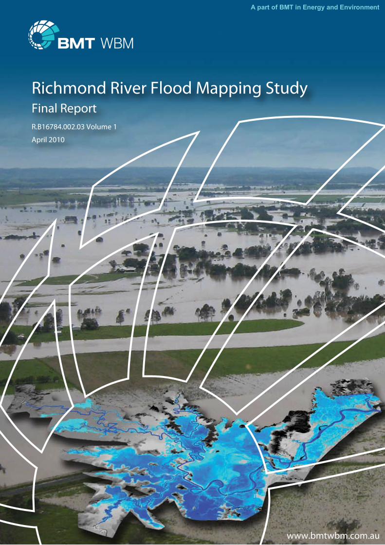
Richmond River Flood Mapping StudyFinal Report R.B16784.002.03 Volume 1
April 2010
A part of BMT in Energy and Environment
www.bmtwbm.com.au
G:\ADMIN\B16784.G.BMC_RICHMONDMEGAMODEL\R B16784 002 03_VOL1.DOC
Richmond River Flood Mapping Study
Volume 1
Final Report
Prepared For: Richmond River County Council
Prepared By: BMT WBM Pty Ltd (Member of the BMT group of companies)
Offices
Brisbane Denver
Melbourne Newcastle
Perth Sydney
Vancouver
G:\ADMIN\B16784.G.BMC_RICHMONDMEGAMODEL\R B16784 002 03_VOL1.DOC
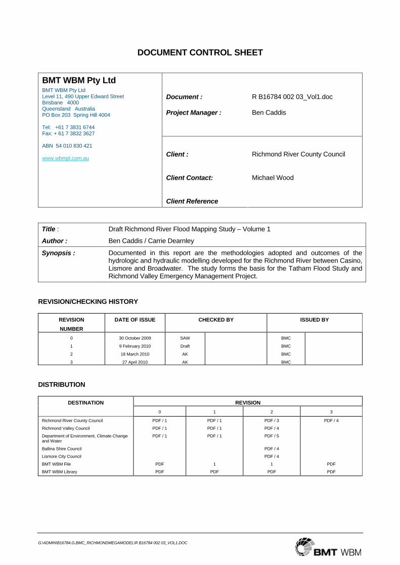
DOCUMENT CONTROL SHEET
Document :
Project Manager :
R B16784 002 03_Vol1.doc
Ben Caddis
BMT WBM Pty Ltd BMT WBM Pty Ltd Level 11, 490 Upper Edward Street Brisbane 4000 Queensland Australia PO Box 203 Spring Hill 4004 Tel: +61 7 3831 6744 Fax: + 61 7 3832 3627 ABN 54 010 830 421 www.wbmpl.com.au
Client :
Client Contact:
Client Reference
Richmond River County Council
Michael Wood
Title : Draft Richmond River Flood Mapping Study – Volume 1
Author : Ben Caddis / Carrie Dearnley
Synopsis : Documented in this report are the methodologies adopted and outcomes of the hydrologic and hydraulic modelling developed for the Richmond River between Casino, Lismore and Broadwater. The study forms the basis for the Tatham Flood Study and Richmond Valley Emergency Management Project.
REVISION/CHECKING HISTORY
REVISION NUMBER
DATE OF ISSUE CHECKED BY ISSUED BY
0 30 October 2009 SAW BMC
1
2
3
9 February 2010
18 March 2010
27 April 2010
Draft
AK
AK
BMC
BMC
BMC
DISTRIBUTION
DESTINATION REVISION
0 1 2 3
Richmond River County Council
Richmond Valley Council
Department of Environment, Climate Change and Water
Ballina Shire Council
Lismore City Council
BMT WBM File
BMT WBM Library
PDF / 1
PDF / 1
PDF / 1
PDF / 1
PDF / 1
PDF / 1
1
PDF / 3
PDF / 4
PDF / 5
PDF / 4
PDF / 4
1
PDF / 4
FOREWORD I
G:\ADMIN\B16784.G.BMC_RICHMONDMEGAMODEL\R B16784 002 03_VOL1.DOC
FOREWORD
The New South Wales government’s Flood Prone Land Policy is directed towards providing solutions to existing flooding problems in developed areas and ensuring that new development is compatible with the flood hazard and does not create additional flooding problems in other areas. Policy and practice are defined in the New South Wales Floodplain Development Manual (2005).
Under the policy, the management of flood prone land remains the responsibility of Local Government. The State Government subsidises flood mitigation works to alleviate existing problems and provides specialist technical advice to assist Councils in their floodplain management responsibilities.
The policy provides for technical and financial support by the State Government through the following four sequential stages:
Stages of Floodplain Risk Management Process
Stage Description
1. Flood Study Determines the nature and extent of the flood problem.
2. Floodplain Risk Management Study Evaluates management options for the floodplain in consideration of social, ecological and economic factors.
3. Floodplain Risk Management Plan Involves formal adoption by Council of a plan of management with preferred options for the floodplain.
4. Plan Implementation Implementation of flood mitigation works, response and property modification measures by Council.
This study represents the first stage of the floodplain risk management process. The study is the first of three studies aimed at understanding and managing flooding within the Richmond Valley between Casino, Lismore and Broadwater.
EXECUTIVE SUMMARY I
G:\ADMIN\B16784.G.BMC_RICHMONDMEGAMODEL\R B16784 002 03_VOL1.DOC
EXECUTIVE SUMMARY The Richmond River is one of New South Wales largest coastal rivers. The upper reaches flow in a general north-south direction from its source on the Queensland New South Wales border in the McPherson Ranges through Casino to its confluence with the Wilsons River at Coraki. The river continues south downstream of Coraki until it meets with Bungawalbin Creek, which is the second major tributary of the Richmond River. At this point the river winds in an easterly direction to Woodburn. Downstream of Woodburn the river turns to flow in a north easterly direction passing Broadwater, Wardell and finally Ballina before reaching the ocean. There is a natural constriction in the river and floodplain at the township of Broadwater. This constriction acts to hold floodwaters in the extensive floodplain basin between Broadwater, Woodburn and Coraki. This floodplain basin is known as the Mid-Richmond.
The study area extends upstream from Broadwater to Lismore on the Wilsons River, the lower Bungawalbin and Casino on the Richmond River, encompassing the Mid-Richmond basin. The contributing catchment to Broadwater is characterised by forests in the steeper upper areas and pastures in the remainder, draining an area of approximately 6,400km2. Flooding in the area is dominated by the three major inflows of the Richmond River, Wilsons River and Bungawalbin Creek. These systems and their catchments are considered to be quite different in nature and result in different flooding problems.
A number of artificial structures affect the movement of flood waters over the floodplain in large floods. Of particular interest are the effects of the Tuckombil Canal (which diverts flood waters to the Evans River), the Bagotville Barrage and the many levees throughout the region.
Consideration of options to reduce flooding impacts, and planning for future development requires an understanding of the flood behaviour. Once flood behaviour is understood, a strategic approach to controlling development on flood prone land, assessing the advantages and disadvantages of flood mitigation options, flood proofing properties and buildings, educating and safeguarding communities and protecting the natural environment can be carried out with confidence.
The Mid-Richmond Flood Study (WBM Oceanics, 1999), followed by the Mid-Richmond Floodplain Risk Management Study (WBM Oceanics, 2002) are the two most recent studies which address flooding issues within the study area. Both studies are based on modelling, using appropriate techniques at the time of publication. These studies formed the basis of the Mid Richmond Floodplain Risk Management Plan that was adopted by Richmond Valley Council on 17 February 2004.
Recognising the need for more detailed modelling in the rural floodplain, Richmond River County Council (RRCC) and Richmond Valley Council (RVC) have identified the need for the following three flood-related studies:
Richmond River Rural Areas – High Risk Floodplain Mapping – This study is proposed by Richmond River County Council to enable flood mapping of the large expanse of floodplain between Casino, Lismore and Broadwater and the lower Bungawalbin.
Richmond Flood Modelling and Tatham Flood Study – This study is proposed by Richmond Valley Council to investigate the hydraulic behaviour of the Richmond River floodplain in the gap between the previous Casino and Mid-Richmond Flood Study areas; and
Richmond River Emergency Management Project – This study is again proposed by Richmond Valley Council to produce flood mapping across the local government area downstream of Casino. The flood mapping would then be used for emergency planning purposes;
EXECUTIVE SUMMARY II
G:\ADMIN\B16784.G.BMC_RICHMONDMEGAMODEL\R B16784 002 03_VOL1.DOC
In recognising the synergies between the three projects, RRCC and RVC formed a team, bringing together all stakeholders so that each study could benefit from the coincident work being undertaken for all three.
In 2005, BMT WBM was engaged by RRCC to undertake the data collection for the projects. This first phase was jointly funded by the federal Natural Disaster Mitigation Program (NDMP), the NSW State Government and RRCC.
In January 2008, BMT WBM was again engaged by RRCC to undertake the Richmond River Flood Mapping Study. This study, jointly funded by the NDMP, RRCC, RVC and the NSW Department of Environment, Climate Change and Water (DECCW), is the first of the three identified studies. During this study, hydrologic and hydraulic investigations and modelling have been undertaken, which the two subsequent studies will build upon.
Data Collection The first stage in the study has involved collating all relevant data across the study areas, including existing reports, ground survey, rainfall and streamflow recordings, and flood mark survey. Additional survey was undertaken to fill the gaps where data was limited.
A questionnaire was distributed to Richmond Valley Council residents in 2008 requesting information relevant to previous flooding, in particular, the recent January 2008 flood. Resulting from the questionnaire and further ‘door-to-door’ survey following the May 2009 flood, the existing flood mark database was expanded to over 250 flood marks across the floodplain. These flood marks were a vital component of the model calibration and verification phase using the 2009, 2008, 1974 and 1954 flood events.
Model Development The overall flood model comprises a hydrologic model and a hydraulic model. Firstly, the hydrologic model is developed to estimate the rate of runoff from a given storm event. Although various hydrologic models within the Richmond catchment have previously been produced, the hydrologic model developed is the first model to cover the entire Richmond River catchment.
Secondly, the hydraulic model is developed to simulate the passage of water through the catchment. Inflow hydrographs, estimated using the hydrologic modelling, are applied at the upstream ends of waterways and floodplains, as well as at lateral inflow locations and sub-catchments throughout the hydraulic model. For the study, a dynamically linked one and two-dimensional (1D/2D) hydraulic model has been developed based on a 60m grid cell resolution and covering the following areas:
Richmond River between Casino and Broadwater (not including Casino);
Bungawalbin Creek from approximately 3km downstream of Neileys Lagoon Road to the Richmond River;
Wilsons River from Lismore to Coraki (not including Lismore); and
Lower reaches of other major tributaries of the Richmond River, such as Shannon Brook (Deep Creek) and Sandy Creek.
In addition to these areas, the model extends along the Richmond River and Evans River to the ocean using a 1D and broadscale 2D approach. In total, the model includes approximately 160km of river and 210km of major creeks.
Model Calibration and Verification To establish a degree of confidence that the models are suitably representing actual site conditions, the models have been calibrated to the November 1994 tidal cycle and the May 2009 flood event. Further validation was performed using the January 2008, March 1974 and February 1954 flood events.
The performance of the model is assessed against the following data:
EXECUTIVE SUMMARY III
G:\ADMIN\B16784.G.BMC_RICHMONDMEGAMODEL\R B16784 002 03_VOL1.DOC
Recorded flood levels and flows at gauging stations;
Peak flood levels from field survey;
Photographs and videos; and
Anecdotal evidence of flood behaviour.
Generally, a reasonable calibration has been achieved. Inaccuracies are largely attributed to the poor availability of recorded rainfall and streamflow data from the southern half of the catchment, in particular, the Bungawalbin.
Design Event Modelling Following model calibration, design events have been used to establish an understanding of the flooding that can be expected to occur during different time periods. For example, a 100 year average recurrence interval (ARI) storm event is a theoretical event that can be expected to occur, on average, once every 100 years.
For this study, the 20, 50, 100 and 500 year ARI events have been assessed, together with the probable maximum flood. The critical duration for each event has been assessed as being either 48 or 72 hour for different parts of the floodplain. Flood mapping has been produced based on the combined 48 and 72 hour durations for each ARI event showing:
Peak flood levels (m AHD);
Peak flood depths (m);
Velocity at peak flood level (m/s);
NSW flood hazard category (based on the NSW Floodplain Development Manual, 2005); and
Flood hazard categories based on velocity depth product (m2/s).
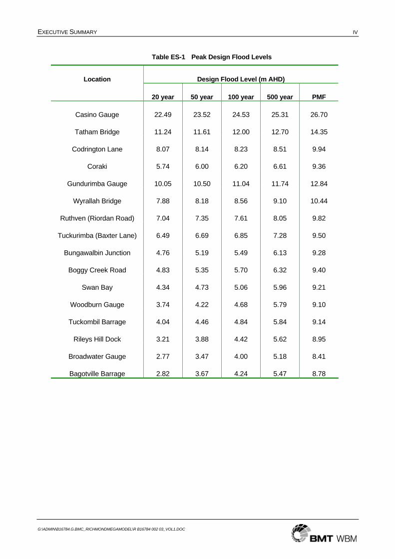
Design flood levels at Coraki, Woodburn and Broadwater have been compared against the results of the flood frequency analyses undertaken during the Mid-Richmond Flood Study (WBM Oceanics, 1999) and Ballina Flood Study Update (BMT WBM, 2008). A good agreement is shown. Refer to Table ES-1 for peak design flood levels throughout the study area.
Two climate change scenarios are also presented based on current projections for increases in rainfall intensity and sea level rise. Although sea level rise is shown to have minimal impact on peak flood levels upstream from Broadwater, increases in rainfall intensity have a significantly larger impact.
EXECUTIVE SUMMARY IV
G:\ADMIN\B16784.G.BMC_RICHMONDMEGAMODEL\R B16784 002 03_VOL1.DOC
Table ES-1 Peak Design Flood Levels
Design Flood Level (m AHD) Location
20 year 50 year 100 year 500 year PMF
Casino Gauge 22.49 23.52 24.53 25.31 26.70
Tatham Bridge 11.24 11.61 12.00 12.70 14.35
Codrington Lane 8.07 8.14 8.23 8.51 9.94
Coraki 5.74 6.00 6.20 6.61 9.36
Gundurimba Gauge 10.05 10.50 11.04 11.74 12.84
Wyrallah Bridge 7.88 8.18 8.56 9.10 10.44
Ruthven (Riordan Road) 7.04 7.35 7.61 8.05 9.82
Tuckurimba (Baxter Lane) 6.49 6.69 6.85 7.28 9.50
Bungawalbin Junction 4.76 5.19 5.49 6.13 9.28
Boggy Creek Road 4.83 5.35 5.70 6.32 9.40
Swan Bay 4.34 4.73 5.06 5.96 9.21
Woodburn Gauge 3.74 4.22 4.68 5.79 9.10
Tuckombil Barrage 4.04 4.46 4.84 5.84 9.14
Rileys Hill Dock 3.21 3.88 4.42 5.62 8.95
Broadwater Gauge 2.77 3.47 4.00 5.18 8.41
Bagotville Barrage 2.82 3.67 4.24 5.47 8.78
CONTENTS V
G:\ADMIN\B16784.G.BMC_RICHMONDMEGAMODEL\R B16784 002 03_VOL1.DOC
CONTENTS
Foreword i Executive Summary i Contents v List of Figures viii List of Tables ix Glossary xi Abbreviations xiv
1 INTRODUCTION 1-1
1.1 Study Background 1-1 1.2 Previous Studies 1-2 1.3 Purpose of Study 1-3 1.4 Study Methodology 1-3 1.5 Stakeholder Consultation 1-4
2 STUDY AREA 2-1
2.1 Catchment Overview 2-1 2.2 Richmond River Catchment 2-1 2.3 Wilsons River Catchment 2-2 2.4 Bungawalbin Creek Catchment 2-2 2.5 Flood Mapping Study Area 2-2 2.6 Flood Structures 2-3
3 DATA COLLECTION 3-1
3.1 Aerial Photography 3-1 3.2 Topographical Survey 3-1
3.2.1 Aerial Survey 3-1 3.2.2 Ground Survey 3-1
3.3 Hydrographic Survey 3-2 3.4 Flood Level Survey 3-2 3.5 Rainfall, Streamflow and Tidal Data 3-3 3.6 Structures 3-3
4 MODEL DEVELOPMENT 4-1
CONTENTS VI
G:\ADMIN\B16784.G.BMC_RICHMONDMEGAMODEL\R B16784 002 03_VOL1.DOC
4.1 Summary 4-1 4.2 Hydrologic Model Development 4-1
4.2.1 Modelling Approach 4-1 4.2.2 Modelling Parameters and Losses 4-2 4.2.3 Major Dams 4-2
4.3 Hydraulic Model Development 4-3 4.3.1 General Modelling Approach 4-3 4.3.2 1D Domain 4-3 4.3.3 2D Domain 4-4 4.3.4 Topography 4-4 4.3.5 Surface Roughness 4-4 4.3.6 Boundary Conditions 4-4
4.4 Model Calibration and Verification 4-5 4.5 Design Event Modelling 4-5
5 MODEL CALIBRATION AND VERIFICATION 5-1
5.1 Calibration and Verification Process 5-1 5.2 Historical Flood Event Selection 5-2
5.2.1 Summary 5-2 5.2.2 May 2009 Flood 5-2 5.2.3 January 2008 Flood 5-3 5.2.4 March 1974 Flood 5-3 5.2.5 February 1954 Flood 5-4
5.3 November 1994 Tidal Calibration 5-4 5.4 Hydrologic Modelling Parameters 5-5 5.5 May 2009 Event Calibration 5-7
5.5.1 Rainfall 5-7 5.5.2 Hydrologic Model Calibration 5-9 5.5.3 Hydraulic Model Calibration 5-14
5.6 January 2008 Event Verification 5-17 5.6.1 Rainfall 5-17 5.6.2 Hydrologic Model Verification 5-19 5.6.3 Hydraulic Model Verification 5-24
5.7 March 1974 Event Verification 5-27 5.7.1 Rainfall 5-27 5.7.2 Changes to the Catchment Since 1974 5-29 5.7.3 Hydrologic Model Verification 5-29
CONTENTS VII
G:\ADMIN\B16784.G.BMC_RICHMONDMEGAMODEL\R B16784 002 03_VOL1.DOC
5.7.4 Hydraulic Model Verification 5-34 5.8 February 1954 Event Verification 5-37
5.8.1 Rainfall 5-37 5.8.2 Changes to Catchment Since 1954 5-37 5.8.3 Hydraulic Model Verification 5-38
5.9 Calibration and Verification Summary 5-38
6 DESIGN EVENT MODELLING 6-1
6.1 Introduction 6-1 6.2 Design Event Hydrology 6-1
6.2.1 Design Rainfall 6-1 6.2.2 PMF Estimation 6-3 6.2.3 Design Losses 6-4 6.2.4 Areal Reduction Factors 6-4 6.2.5 Joint Probability 6-5
6.3 Critical Duration Analysis 6-6 6.4 Design Flood Mapping 6-6
6.4.1 20 Year ARI 6-7 6.4.2 50 Year ARI 6-7 6.4.3 100 Year ARI 6-8 6.4.4 500 Year ARI 6-8 6.4.5 Probable Maximum Flood 6-8
6.5 Design Flood Level Summary 6-9 6.6 Flood Frequency Analysis 6-10 6.7 Sensitivity Analysis 6-11 6.8 Climate Change Assessment 6-12
7 CONCLUSION 7-1
8 ACKNOWLEDGEMENTS 8-1
9 REFERENCES 9-1
APPENDIX A: DISCUSSION PAPER ON SURVEY DATA A-1
APPENDIX B: TIDAL CALIBRATION RESULTS B-1
LIST OF FIGURES VIII
G:\ADMIN\B16784.G.BMC_RICHMONDMEGAMODEL\R B16784 002 03_VOL1.DOC
LIST OF FIGURES
Figure 5-1 May 2009 Cumulative Rainfall 5-8 Figure 5-2 May 2009 Normalised Cumulative Rainfall 5-8 Figure 5-3 May 2009 Wiangaree Hydrologic Calibration 5-10 Figure 5-4 May 2009 Kyogle Hydrologic Calibration 5-10 Figure 5-5 May 2009 Casino Hydrologic Calibration 5-11 Figure 5-6 May 2009 Rock Valley Hydrologic Calibration 5-11 Figure 5-7 May 2009 Ewing Hydrologic Calibration 5-12 Figure 5-8 May 2009 Eltham Hydrologic Calibration 5-12 Figure 5-9 May 2009 Lismore Hydrologic Calibration 5-13 Figure 5-10 May 2009 Rappville Hydrologic Calibration 5-13 Figure 5-11 May 2009 Gundurimba Hydraulic Calibration 5-15 Figure 5-12 May 2009 Coraki Hydraulic Calibration 5-15 Figure 5-13 May 2009 Bungawalbin Junction Hydraulic Calibration 5-16 Figure 5-14 May 2009 Woodburn Hydraulic Calibration 5-16 Figure 5-15 January 2008 Cumulative Rainfall 5-18 Figure 5-16 January 2008 Normalised Cumulative Rainfall 5-18 Figure 5-17 January 2008 Wiangaree Hydrologic Verification 5-20 Figure 5-18 January 2008 Kyogle Hydrologic Verification 5-20 Figure 5-19 January 2008 Casino Hydrologic Verification 5-21 Figure 5-20 January 2008 Yorklea Hydrologic Verification 5-21 Figure 5-21 January 2008 Binna Burra Hydrologic Verification 5-22 Figure 5-22 January 2008 Eltham Hydrologic Verification 5-22 Figure 5-23 January 2008 Lismore Hydrologic Verification 5-23 Figure 5-24 January 2008 Rappville Hydrologic Verification 5-23 Figure 5-25 January 2008 Gundurimba Hydraulic Verification 5-25 Figure 5-26 January 2008 Coraki Hydraulic Verification 5-25 Figure 5-27 January 2008 Bungawalbin Junction Hydraulic Verification 5-26 Figure 5-28 January 2008 Woodburn Hydraulic Verification 5-26 Figure 5-29 January 2008 Byrnes Point Hydraulic Verification 5-27 Figure 5-30 March 1974 Cumulative Rainfall 5-28 Figure 5-31 March 1974 Normalised Cumulative Rainfall 5-28 Figure 5-32 March 1974 Wiangaree Hydrologic Verification 5-30 Figure 5-33 March 1974 Kyogle Hydrologic Verification 5-30 Figure 5-34 March 1974 Casino Hydrologic Verification 5-31 Figure 5-35 March 1974 Rock Valley Hydrologic Verification 5-31 Figure 5-36 March 1974 Keerong Hydrologic Verification 5-32 Figure 5-37 March 1974 Eltham Hydrologic Verification 5-32 Figure 5-38 March 1974 Lismore Hydrologic Verification 5-33
LIST OF TABLES IX
G:\ADMIN\B16784.G.BMC_RICHMONDMEGAMODEL\R B16784 002 03_VOL1.DOC
Figure 5-39 March 1974 Teven Hydrologic Verification 5-33 Figure 5-40 March 1974 Coraki Hydraulic Verification 5-35 Figure 5-41 March 1974 Bungawalbin Junction Hydraulic Verification 5-35 Figure 5-42 March 1974 Woodburn Hydraulic Verification 5-36 Figure 5-43 March 1974 Broadwater Hydraulic Verification 5-36 Figure 5-44 March 1974 Wardell Hydraulic Verification 5-37
Figure B-1 Site 1: Richmond River Entrance - Water Levels B-1 Figure B-2 Site 1: Richmond River Entrance – Discharge B-1 Figure B-3 Site 5: Missingham Bridge – Water Levels B-2 Figure B-4 Site 5: Missingham Bridge – Discharge B-2 Figure B-5 Site 7: Burns Point – Water Levels B-3 Figure B-6 Site 13: Broadwater – Water Levels B-3 Figure B-7 Site 13: Broadwater – Discharge B-4 Figure B-8 Site 14: Woodburn – Water Levels B-4 Figure B-9 Site 18: Richmond River at Coraki – Water Levels B-5 Figure B-10 Site 25: Richmond River at Coraki – Discharge B-5 Figure B-11 Site 26: Tatham Bridge – Water Levels B-6 Figure B-12 Site 27: Tomki Bight Road – Water Levels B-6 Figure B-13 Site 3: North Creek Canal – Water Levels B-7 Figure B-14 Site 4: North Creek Road – Water Levels B-7 Figure B-15 Site 11: Tuckean Broadwater Barrage – Water Levels B-8 Figure B-16 Site 10: Tuckean Broadwater Barrage – Discharge B-8 Figure B-17 Site 19: Wilsons River at Coraki – Water Levels B-9 Figure B-18 Site 19: Wilsons River at Coraki – Discharge B-9 Figure B-19 Site 16: Rocky Mouth Creek at Pacific Highway – Water Levels B-10 Figure B-20 Site 17: Rocky Mouth Creek Floodgates – Water Levels B-10 Figure B-21 Site 20: Wilsons River at Lismore Airport – Water Levels B-11 Figure B-22 Site 21: Wilsons River at Lismore Airport - Discharge B-11
LIST OF TABLES
Table 3-1 Recorded Flood Levels 3-3 Table 5-1 Historical Event Lag Times – Upper Richmond 5-6 Table 5-2 Historical Event Lag Times – Wilsons 5-6 Table 5-3 Peak Flood Level Comparison 5-39 Table 5-4 Manning’s ‘n’ Roughness 5-39 Table 6-1 Terminology Used for Design Floods 6-1 Table 6-2 100 Year ARI Design Event Peak Flow Rates 6-3

LIST OF TABLES X
G:\ADMIN\B16784.G.BMC_RICHMONDMEGAMODEL\R B16784 002 03_VOL1.DOC
Table 6-3 Comparison of Design Rainfall Depths 6-4 Table 6-4 Areal Reduction Factors Based on CRCCH Method 6-5 Table 6-5 Design Rainfall and Storm Surge 6-6 Table 6-6 Peak Design Flood Levels 6-9 Table 6-7 Peak Flood Levels at Coraki 6-10 Table 6-8 Peak Flood Levels at Woodburn 6-10 Table 6-9 Peak Flood Levels at Broadwater 6-11 Table 6-10 Climate Change Scenario Results 6-13
GLOSSARY XI
G:\ADMIN\B16784.G.BMC_RICHMONDMEGAMODEL\R B16784 002 03_VOL1.DOC
GLOSSARY Australian Height Datum (AHD)
Common national survey datum corresponding approximately to mean sea level.
Average Recurrence Interval (ARI)
The long-term average number of years between the occurrence of a flood as big as (or larger than) the selected event. For example, floods with a discharge as great as (or greater than) the 20yr ARI design flood will occur on average once every 20 years. ARI is another way of expressing the likelihood of occurrence of a flood event.
Catchment The area of land draining through the main stream (as well as tributary streams) to a particular site. It always relates to an area upstream of a specific location.
Cumec Measure of discharge. Cubic metres per second.
Depth The height or the elevation of floodwaters above ground level (in metres). Not to be confused with water level, which is the height of the water relative to a datum (not ground level).
Design flood A hypothetical flood representing a specific likelihood of occurrence (for example the 100 year ARI or 1% AEP flood).
Discharge The flow within a watercourse usually expressed as cubic metres per second (cumecs). Also referred to as flow.
Flood Relatively high river, creek, estuary, lake or dam flows, which overtop the natural or artificial banks, and inundate floodplains, and/or local overland flooding associated with drainage before entering a watercourse, and/or coastal inundation resulting from super elevated sea levels and/or waves overtopping coastline defences excluding tsunami.
Flood behaviour The pattern, characteristics and nature of a flood.
Flood fringe areas Flood prone land that is not designated as floodway or flood storage areas.
Flood level The height or elevation of floodwaters relative to a datum (typically the Australian Height Datum). Also referred to as “stage”.
Flood liable land Land susceptible to flooding by the PMF event (see also Flood Prone Land). Flood liable land covers the whole floodplain, not just that part below the flood planning levels.
Flood prone land Land susceptible to inundation by the probable maximum flood (PMF) event. See also flood liable land.
Flood storage areas Floodplain areas that are important for the temporary storage of floodwaters during the passage of a flood. The extent and behaviour of flood storage areas may change with flood severity. Loss of flood storage can increase the severity of flood impacts by reducing natural flood attenuation. Hence it is necessary to investigate a range of flood events before defining flood storage areas.
GLOSSARY XII
G:\ADMIN\B16784.G.BMC_RICHMONDMEGAMODEL\R B16784 002 03_VOL1.DOC
Floodplain Area of land subject to inundation by floods up to and including the probable maximum flood (PMF) event, i.e. flood prone land.
Floodplain management The co-ordinated management of activities that occur on the floodplain.
Floodway areas Floodplain areas carrying significant volumes (discharges) of floodwaters during a flood. They are often aligned with natural channels. Partial blockage of floodway areas would cause a significant redistribution of flood flows, or a significant increase in flood levels.
Hazard A source of potential harm or a situation with a potential to cause loss. Flooding is a hazard which has the potential to cause damage to the community. The degree of flood hazard varies with circumstances across the full range of floods. Refer to Floodplain Development Manual (2005) for definition of high and low hazard categories.
Historical flood A flood that has actually occurred in the past.
Hydraulics The term given to the study of water flow in waterways (i.e. rivers, estuaries and coastal systems).
Hydrograph A graph showing how the discharge or stage/flood level at any particular location varies with time during a flood.
Hydrology The term given to the study of the rainfall-runoff processes in catchments.
Peak flood level, flow or velocity
The maximum flood level, flow (i.e. discharge) or velocity that occurs during a flood event.
Probable Maximum Flood (PMF)
An extreme flood deemed to be the largest flood that could conceivably occur at a specific location. It is generally not physically or economically possible to provide complete protection against this flood event, but should be considered for emergency response etc. The PMF defines the extent of flood prone land (i.e. the floodplain).
Probability A statistical measure of the likely frequency or occurrence of flooding. See also AEP.
Risk The chance of something happening that will have an impact, usually measured in terms of both the likelihood of something happening, as well as the consequences of that thing happening.
RORB A hydrologic model (software) used to simulate the catchment rainfall-runoff process, including the amount of runoff from rainfall, and the attenuation of the flood wave as it travels down a catchment.
Runoff The amount of rainfall from a catchment that actually ends up as flowing water in the river or creek, also known as rainfall excess.
Stage Equivalent to water level. See flood level.
Stage hydrograph A graph showing the evolution of water level at a particular location over time during a flood.
GLOSSARY XIII
G:\ADMIN\B16784.G.BMC_RICHMONDMEGAMODEL\R B16784 002 03_VOL1.DOC
TUFLOW 1D and 2D hydraulic model (software). It simulates the complex hydrodynamics of floods and tides using the full 1D St Venant equations and the full 2D free-surface shallow water equations.
Velocity The speed at which floodwaters are moving (in metres per second). A flood velocity predicted by a 2D computer flood model is quoted as the depth averaged velocity, i.e. the average velocity throughout the depth of the water column. A flood velocity predicted by a 1D or quasi-2D computer flood model is quoted as the depth and width averaged velocity, i.e. the average velocity across the whole river or creek section.
Velocity-depth product The velocity of floodwaters multiplied by the depth (in metres squared per second). Also equivalent to the flow per unit width.
Water level See flood level.
WBNM (Watershed Bounded Network Model)
A hydrologic model (software) used to simulate the catchment rainfall-runoff process, including the amount of runoff from rainfall, and the attenuation of the flood wave as it travels down a catchment.

ABBREVIATIONS XIV
G:\ADMIN\B16784.G.BMC_RICHMONDMEGAMODEL\R B16784 002 03_VOL1.DOC
ABBREVIATIONS 1D / 2D One dimensional / two dimensional
AHD Australian Height Datum
ALS Airborne Laser Scanning
ARI Average Recurrence Interval
ARR Australian Rainfall and Runoff (IEAust, 1987)
BOM Bureau of Meteorology
BSC Ballina Shire Council
DECCW Department of Environment, Climate Change and Water
DEM Digital Elevation Model
DIPNR Department of Infrastructure, Planning and Natural Resources
DLWC Department of Land and Water Conservation
DEM Digital Elevation Model
DWE Department of Water and Energy (now part of DECCW)
GIS Geographical Information System
GSDM Generalised Short Duration Method
GTSMR Generalised Tropical Storm Method (Revised)
km Kilometre
LCC Lismore City Council
m Metre
m/s Metres per second
m3/s Cubic metres per second
mAHD Elevation in metres relative to the Australian Height Datum
PMP Probable Maximum Precipitation
PMF Probable Maximum Flood
PWD Public Works Department (now Department of Commerce)
RRCC Richmond River County Council
RVC Richmond Valley Council
TIN Triangulated Irregular Network

ABBREVIATIONS XV
G:\ADMIN\B16784.G.BMC_RICHMONDMEGAMODEL\R B16784 002 03_VOL1.DOC
V x D Velocity-depth product
WBNM Watershed Network Bounded Model (see Glossary)
INTRODUCTION 1-1
G:\ADMIN\B16784.G.BMC_RICHMONDMEGAMODEL\R B16784 002 03_VOL1.DOC
1 INTRODUCTION
1.1 Study Background
Richmond River County Council (RRCC) and Richmond Valley Council (RVC) have previously identified the need for the following three flood-related studies:
Richmond River Rural Areas – High Risk Floodplain Mapping – This study is proposed by Richmond River County Council to enable flood mapping of the large expanse of floodplain between Casino, Lismore and Broadwater.
Tatham Flood Study – This study is proposed by Richmond Valley Council to investigate the hydraulic behaviour of the Richmond River floodplain in the gap between the previous Casino and Mid-Richmond Flood Study areas; and
Richmond River Emergency Management Project – This study is again proposed by Richmond Valley Council to produce flood mapping across the local government area downstream of Casino. The flood mapping would then be used for emergency planning purposes;
In recognising the synergies between the three projects, RRCC and RVC formed a team, bringing together all stakeholders so that each study could benefit from the coincident work being undertaken for all three.
In 2005, BMT WBM was engaged by RRCC to undertake the data collection for the projects. This first phase was jointly funded by the federal Natural Disaster Mitigation Program (NDMP), the NSW State Government and RRCC.
In January 2008, BMT WBM was again engaged by RRCC to undertake the Richmond River Flood Mapping Study. This study, jointly funded by the NDMP, RRCC, RVC and the NSW Department of Environment, Climate Change and Water (DECCW), is the first of the three identified studies. During this study, hydrologic and hydraulic investigations and modelling have been undertaken, which the two subsequent studies will build upon.
For the study, a dynamically linked one and two-dimensional (1D/2D) flood model has been developed for the following areas:
Richmond River between Casino and Broadwater (not including Casino);
Bungawalbin Creek from approximately 3km downstream of Neileys Lagoon Road to the Richmond River;
Wilsons River from Lismore to Coraki (not including Lismore); and
Lower reaches of other major tributaries of the Richmond River, such as Shannon Brook (Deep Creek) and Sandy Creek.
In addition to these areas, the model will be extended along the Richmond River and Evans River to the ocean using a 1D and broadscale 2D approach. In total, the model will include approximately 160km of river and 210km of major creeks.
INTRODUCTION 1-2
G:\ADMIN\B16784.G.BMC_RICHMONDMEGAMODEL\R B16784 002 03_VOL1.DOC
1.2 Previous Studies
Since devastating floods in 1954, the Richmond Valley has been the subject of numerous flood investigations and floodplain management studies. Most of these studies have focussed either on the construction and management of the myriad of flood and drainage management structures across the valley, or the forecasting and warning of potential floods. Three of the early studies which include flood mapping of the 1954 event include:
Report of the Richmond River Valley Flood Mitigation Committee (Department of Public Works, 1954 & 1958);
NSW Coastal Rivers Flood Plain Management Studies, Richmond Valley (Sinclair Knight and Partners, 1980); and
Richmond Valley Flood Problems (Richmond River Inter-Departmental Committee, 1982).
In more recent years, hydrologic and hydraulic models have been used to gain a better understanding of local flood behaviour. These models have then been used to assess the benefits and impacts of various mitigation measures across the floodplain.
Some of these more recent studies, reporting on the outcomes of detailed modelling include:
Lismore Flood Study and Floodplain Management (Sinclair Knight Merz ,1993);
Ballina Floodplain Management Study (WBM Oceanics, 1997);
Casino Flood Study (WBM Oceanics, 1998);
Lismore Levee Scheme Environmental Impact Statement (WBM Oceanics, 1999);
Mid-Richmond Flood Study (WBM Oceanics, 1999);
Casino Floodplain Risk Management Study (WBM Oceanics, 2001);
Lismore Floodplain Management Study (Patterson Britton, 2001);
Mid-Richmond Floodplain Management Study (WBM Oceanics, 2002);
Wardell and Cabbage Tree Island Floodplain Management Study (Patterson Britton, 2004);
Tuckombil Canal Flood Affect Assessment (WBM Oceanics 2005); and
Ballina Flood Study Update (BMT WBM, 2008).
In preparation for the Richmond River Flood Mapping Study, RRCC engaged BMT WBM to prepare the Richmond River Data Compilation Study (WBM, 2006). That study aimed at collating information pertaining to:
Historical and design flooding (levels, depths, velocities, hazard and discharge);
Historical and design rainfall;
Floor levels;
Watercourse cross sections and bathymetry; and
Aerial and ground survey.
INTRODUCTION 1-3
G:\ADMIN\B16784.G.BMC_RICHMONDMEGAMODEL\R B16784 002 03_VOL1.DOC
That study has formed a significant part of the data collection exercise required for this study.
1.3 Purpose of Study
Modelling undertaken as part of the previous studies has used various software. Each study has taken advantage of technological advances in modelling techniques and computer processing time. In addition, the latest data and guidelines were used for each study.
Prior to 2001, most river and floodplain modelling was undertaken using one-dimensional (1D) techniques. Channels and flowpaths were typically represented as a series of interconnected 1D links. Subsequent development of two-dimensional (2D) and integrated 1D/2D modelling software generally replaced the use of 1D software for modelling complex flow behaviour. The use of 2D and 1D/2D models has enabled a far superior representation and understanding of flood behaviour.
The previously developed 2D models of Lismore, Casino, and Wardell and Cabbage Tree Island are of importance to this study, as they form the extents of the current study area. Hence, the 1D and 1D/2D modelling previously undertaken for the Mid-Richmond and Tuckombil Canal studies respectively, will be superseded by a 1D/2D model covering the floodplain between Casino, Lismore and Broadwater.
The key deliverables from this project are:
1 A calibrated hydrologic model covering the entire Richmond River catchment;
2 A calibrated 1D/2D hydraulic model of the floodplain between Casino, Lismore and Broadwater;
3 A comprehensive understanding of flood behaviour across the study area; and
4 Flood mapping of historical and design flood events, in particular flood levels and hazards.
The models developed as part of this project will be used for the Tatham Flood Study and the Richmond Valley Emergency Management Project. It is intended to develop robust models that can be used and further developed for a range of future applications; in particular, to aid floodplain management decisions.
1.4 Study Methodology
The general approach employed to achieve the study objectives involves the following steps:
Compilation and review of available information;
Acquisition of additional data to determine nature and extent of historical flooding;
Development of hydrological and hydraulic models;
Calibration and verification of models to historical flood events;
Modelling of design events under existing conditions; and
Reporting and mapping.
The above tasks are described in detail in the following sections.
INTRODUCTION 1-4
G:\ADMIN\B16784.G.BMC_RICHMONDMEGAMODEL\R B16784 002 03_VOL1.DOC
1.5 Stakeholder Consultation
During the early stages of this study, the project team recognised that effective engagement with the project stakeholder groups could significantly enhance the outcomes of the study. Two stakeholder groups were identified:
Local community; generally comprising local land owners and residents; and
Local authorities; generally comprising local Councils, state government departments and the emergency services.
Prior to issue of the draft report, two stakeholder presentations were held:
1. Local Authorities - 29 July 2009 at the Coraki Conference Centre
Delegates of the presentation included:
Richmond River County Council;
Richmond Valley Council;
Lismore City Council;
Ballina Shire Council;
Local and regional SES officers;
NSW Department of Planning;
NSW Parks and Wildlife; and
Southern Cross University.
The purpose of the presentation was to inform the stakeholders regarding the objectives and status of the project.
2. Local Community – 24 November 2009 at the Coraki Conference Centre
Local community members who had contributed information during the data collection phase of the project were invited to attend the presentation. The purpose of the presentation was initially to thank the community for their assistance before providing the attendees details of the objectives and status of the project. The results of the initial model calibration were presented and feedback requested. The subsequent information provided was used to further refine the model calibration.
STUDY AREA 2-1
G:\ADMIN\B16784.G.BMC_RICHMONDMEGAMODEL\R B16784 002 03_VOL1.DOC
2 STUDY AREA
2.1 Catchment Overview
Located within the Northern Rivers region of New South Wales, the Richmond River catchment covers an area of approximately 6,900km2. The catchment is bound by the Logan, Tweed and Brunswick River catchments to the north, the Clarence River to the west and south, and the Pacific Ocean to the east. Refer to Map 2-1 and Map 2-2 for locality and study area.
Topographically, the catchment is typical of the region. Steep mountainous ranges line the upper reaches of the catchment, falling to the flat floodplains of the mid and lower parts of the catchment. Elevations range from sea level to greater than 1,000m within the Richmond and McPherson Ranges. The Richmond River system comprises three main drainage basins; the Richmond River, Wilsons River and Bungawalbin Creek. These basins are discussed in the following sections.
Hydraulically linked to the Richmond River catchment is the relatively small catchment of the Evans River. The Tuckombil Canal is a manmade waterway that links the Evans River to Rocky Mouth Creek, two kilometres upstream of the confluence with the Richmond River at Woodburn. At the northern extent of the canal, the Tuckombil Barrage prevents tidal intrusion into Rocky Mouth Creek, whilst providing flood relief for the Richmond River.
Landuse across the Richmond Valley is predominantly characterised by forests in the steeper upper areas and pasture and cropping in the remainder.
2.2 Richmond River Catchment
The Richmond is initially a series of steep mountain streams which combine forming a major flow path at Wiangaree. As the river flattens out, it exhibits meandering patterns and the floodplain starts to become more pronounced as the river passes through Kyogle towards Casino. The river through Casino is effectively a gorge with high banks, exposed rock beds and river bed levels dropping over 8m through town. Under very large flood events, waters break the banks upstream of Casino and bypass the town via a large flow path to the south. On the downstream (eastern) side of Casino, the topography flattens out to form an extensive floodplain as the major system of Shannon Brook enters at Tatham and continues towards Coraki.
After flowing through the rural areas of Tatham and Codrington, the Richmond River is joined by the Wilsons River at Coraki. Downstream of Coraki, the river approximately doubles in width to over 200m. The river then winds in a southerly direction to its confluence with its second largest tributary, Bungawalbin Creek at Bungawalbin Junction. From Bungawalbin Junction, the river flows past Swan Bay to Woodburn, and then in a north easterly direction, parallel to the coastline. The river passes the towns of Broadwater and Wardell, before reaching the Pacific Ocean at Ballina.
A natural constriction in the river and floodplain at the township of Broadwater acts to hold floodwaters in the extensive floodplain ‘basin’ between Broadwater, Woodburn and Coraki. This part of the floodplain is known as the Mid-Richmond. Flooding in the Mid-Richmond area is dominated by the three major inflows of the Richmond River, Wilsons River and Bungawalbin Creek.
STUDY AREA 2-2
G:\ADMIN\B16784.G.BMC_RICHMONDMEGAMODEL\R B16784 002 03_VOL1.DOC
The tidal extents of the Richmond River extend almost as far as Casino, 108km upstream from the river entrance at Ballina.
2.3 Wilsons River Catchment
The Wilsons River is the larger of the two major tributaries of the Richmond River, covering a catchment of 1,500km2. The majority of the catchment is located upstream of Lismore (1,400km2). Lismore itself is located at the confluence of the Wilsons River and Leycester Creek; the latter comprising 900km2 of the catchment. The catchment is dominated by long, narrow, steep valleys running in a general north to south direction forming what was, millions of years ago, the slopes of a large volcano, which is now Mount Warning.
Due to its location at a natural constriction of a major river system, Lismore has a long history of flooding. Downstream of Lismore, the Wilsons River meanders in a southerly direction through the rural areas of Gundurimba, Wyrallah and Tuckurimba. The Wilsons River then joins the Richmond River at Coraki.
Tidal extents of the Wilsons system are 113km and 115km upstream of the river entrance within the Wilsons River and Terania Creek respectively.
2.4 Bungawalbin Creek Catchment
Bungawalbin Creek is the second major tributary of the Richmond River, draining a catchment of 1,400km2. The system is initially a series of steep mountain streams which flow into the floodplain at the headwaters of Bungawalbin Creek. The creek flows along the edge of this floodplain between Myrtle Creek and Gibberagee, along which a number of tributaries enter. The creek and floodplain constrict approximately 15 kilometres downstream of Gibberagee. At this point, the creek and associated low floodplain areas wind in a north east direction meeting with a major tributary, Sandy Creek, before entering the Richmond River.
The Bungawalbin area serves as a major flood storage basin for the Richmond River. Floodwaters from the Bungawalbin are held until the water level in the Richmond River has receded sufficiently to allow the catchment to drain. In certain events, flood waters from the Richmond River back up into the Bungawalbin.
The tidal extent of Bungawalbin Creek is more than 88km upstream from the river entrance.
2.5 Flood Mapping Study Area
The extent of the 2D flood mapping for this project is shown on Map 2-2. The area covers the following watercourses:
Richmond River from the downstream side of Casino to the Ballina Shire Council (BSC) local government area (LGA) boundary at Broadwater. These extents cover the ‘gap’ between the mapping produced for the Casino Floodplain Risk Management Study (WBM, 2001) and the Wardell and Cabbage Tree Island Study (Patterson Britton, 2004);
STUDY AREA 2-3
G:\ADMIN\B16784.G.BMC_RICHMONDMEGAMODEL\R B16784 002 03_VOL1.DOC
Wilsons River from the downstream side of Lismore to the Richmond River confluence at Coraki. The upstream boundary coincides with the downstream extent of mapping produced for the Lismore Floodplain Management Study (Patterson Britton, 2001);
Bungawalbin Creek from approximately 3km downstream of Neileys Lagoon Road to the Richmond River confluence at Bungawalbin Junction;
Sandy Creek from approximately 3km upstream of the Tatham-Ellangowan Road crossing to the Bungawalbin Creek confluence near Bungawalbin Junction; and
Shannon Brook (formerly known as Deep Creek) from 3km downstream of Yorklea to the Richmond River confluence at Tatham.
2.6 Flood Structures
A number of artificial structures along the Richmond River affect the movement of flood waters over the floodplain in large floods. Of particular importance to this study are the Lismore and Tuckurimba Levees, the Tuckombil Canal and Barrage, Rocky Mouth Creek Floodgates and the Bagotville Barrage as discussed below. Numerous other smaller levees also have a significant role in diverting floodwaters around the floodplain. Refer to Map 2-3 for major hydraulic structure locations.
Lismore Levee – the levee runs along the eastern bank of the Wilsons River alongside the Lismore CBD. Construction was completed in 2005. The levee is designed to have immunity from the 10 year average recurrence interval flood.
Tuckurimba Levee – the levee runs along the eastern bank of the Wilsons River between Baxters Lane and Coraki. The levee was constructed by the Gundurimba ‘C’ Riding Drainage Union in the 1950’s and completed by RRCC in 1964. Properties to the east of the levee are protected from flood waters breaking out of the Wilsons River during more frequent events. Until the levee is breached, floodwaters are also prevented from flowing into the Tuckean Swamp to the east, hence, bypassing the Coraki and Woodburn areas.
Tuckombil Canal and Barrage – the Tuckombil Canal was originally excavated in 1895 between Rocky Mouth Creek and the Evans River. The canal was intended to provide flood relief to the Mid-Richmond area, allowing floodwaters to drain to the ocean via the Evans River. The original construction of the canal had a flagstone causeway slightly above high tide level, to prevent tidal exchange. In 1965, the canal was excavated to its current form. An inflatable fabridam was located at the upstream end. During normal operation, the fabridam remained inflated, thus preventing tidal exchange. The dam was deflated during flood, to maximise the drainage potential of the canal. Following numerous replacements, the fabridam was replaced in 2001 by a temporary fixed concrete weir at 0.94m AHD.
Rocky Mouth Creek Floodgates – a large set of floodgates located on Rocky Mouth Creek are designed to prevent salt water intrusion onto the agricultural land further upstream.
Bagotville Barrage – the barrage is a large floodgated structure built in 1971 to prevent saline water entering the Tuckean Swamp area. The barrage is located at the headwaters of the Tuckean Broadwater.
DATA COLLECTION 3-1
G:\ADMIN\B16784.G.BMC_RICHMONDMEGAMODEL\R B16784 002 03_VOL1.DOC
3 DATA COLLECTION
3.1 Aerial Photography
Orthorectified aerial imagery of the Mid-Richmond area was captured in 2007 as part of the aerial survey undertaken for this project. Aerial photography of the remainder of the study area has been sourced from the various previous studies undertaken for RRCC, RVC and Ballina Shire Council (BSC).
The available imagery has been used for land use mapping and as a background for the flood mapping presented later in this document.
3.2 Topographical Survey
3.2.1 Aerial Survey
Photogrammetric and airborne laser scanning (ALS) survey were made available for this study by local Councils and the NSW Roads and Traffic Authority. Digital elevation models (DEMs) created from these datasets have previously been used for the following projects:
Ballina Flood Study Update (BMT WBM, 2008);
Casino Floodplain Risk Management Study (WBM Oceanics, 2001);
Tuckombil Canal Flood Affect Assessment (WBM Oceanics 2005);
Wardell and Cabbage Tree Island Floodplain Management Study (Patterson Britton, 2004);
Lismore Floodplain Management Study (Patterson Britton, 2001); and
Woodburn to Ballina Pacific Highway Upgrade (Brown Consulting, 2006).
In 2007, aerial survey was captured for the area between the existing datasets.
In 2008, BMT WBM prepared the Draft Discussion Paper on Survey Data as part of this project. The discussion paper summarised the process employed for producing a single DEM for the catchment using the various datasets. Also included in the discussion paper is a summary of the data verification process. The discussion paper is reproduced here as Appendix A.
3.2.2 Ground Survey
Ground survey across the study area has previously been collected for the following studies:
Mid-Richmond Flood Study (WBM, 1998); and
Casino Floodplain Risk Management Study (WBM, 2001).
The survey typically comprises spot heights along hydraulic controls, such as road embankments and levees.
DATA COLLECTION 3-2
G:\ADMIN\B16784.G.BMC_RICHMONDMEGAMODEL\R B16784 002 03_VOL1.DOC
Additionally, control survey of local Permanent Survey Marks (PSMs) was made available by the NSW Department of Lands. The available ground survey, including additional ground survey collected for this study, has been used for the following purposes:
Verification of the aerial survey accuracy; and
Definition of hydraulic controls within the hydraulic model.
For further details, refer to Appendix A.
3.3 Hydrographic Survey
Hydrographic survey of the estuarine extents of the Richmond River system was captured in 2004 as part of the NSW Department of Natural Resources’ (DNR) Estuary Management Program. The survey was provided for this project by the NSW Department of Environment, Climate Change and Water (DECCW). Refer to Appendix A for further discussion on the extents and resolution of the survey.
3.4 Flood Level Survey
Two major floods occurred within the Richmond River between the study inception and finalisation of the model calibration phase. Given the opportunity to undertake extensive field data collection exercises during and following these flood events, and considering the spatial extents and magnitude of the floods, it was decided to include these events for model calibration and verification.
The following events were, therefore, the focus of field data collection:
February 1954;
March 1974;
January 2008; and
May 2009.
Two field data collection exercises were undertaken for the project. The first followed the January 2008 flood, and the second followed the May 2009 flood.
In early 2008, RVC distributed a questionnaire together with the annual rates renewal notices. Residents who had any information relating to the recent or historical flood events were prompted to respond to the questionnaire. Returned questionnaires were subsequently processed by RVC. Residents who had relevant information were contacted and, where necessary, Council surveyors went to the property to survey peak flood levels.
Targeting areas with sparse information, in 2008 BMT WBM engineers undertook a door-knocking exercise to gather any further information.
Following the May 2009 flood, the State Emergency Service (SES), RRCC and BMT WBM collected field data relating to peak flood levels and localised flood behaviour for that event. Again, surveyors were deployed to record peak flood levels.
DATA COLLECTION 3-3
G:\ADMIN\B16784.G.BMC_RICHMONDMEGAMODEL\R B16784 002 03_VOL1.DOC
To summarise, all methods used for the field data collection exercise were successful. The surveyed flood levels are extremely valuable to this study. Flood levels for the 1954 and 1974 events were also extracted from the Mid-Richmond, Casino and Ballina studies. The number of flood levels recorded for each event is listed in Table 3-1. Refer to Map 3-1 for mapping of floor level survey. Refer also to Section 5 for flood levels and model calibration and verification.
Table 3-1 Recorded Flood Levels
Flood Event Number of Flood Levels
May 2009 46
January 2008 78
March 1974 66
February 1954 61
3.5 Rainfall, Streamflow and Tidal Data
Daily, hourly and continuous (5 minute or 6 minute pluviographic) rainfall records were sourced from the Bureau of Meteorology (BOM), DECCW and Manly Hydraulics Laboratory (MHL). The data was collated and mapped spatially to develop an understanding of the spatial and temporal distribution of the rainfall for the four nominated events. Further discussion on the use of the rainfall data is discussed in Section 5.
Streamflow and level recordings were sourced from the BOM and DECCW for a range of gauging stations throughout the catchment. Records of discharge verus time were provided for the watercourses upstream of the tidal extents, and water level over time for the gauges of the lower floodplain. The BOM also provided a rating curve for the Lismore Rowing Club gauge, for conversion of water level to discharge.
Tidal data was sourced from MHL for the January 2008 and February 2009 events. Tidal data for the March 1974 event was used in accordance with the Mid-Richmond Flood Study (WBM, 1999). The tide levels used for that study are based on recordings at Coffs Harbour with an additional 300mm added to account for storm surge. The tide levels used for the February 1954 event were derived synthetically.
3.6 Structures
Work as Executed (WAE) drawings of all major bridge and culvert structures were collated and provided by RVC. This data was supplemented with data used for the Mid-Richmond Flood Study (WBM, 1999).
MODEL DEVELOPMENT 4-1
G:\ADMIN\B16784.G.BMC_RICHMONDMEGAMODEL\R B16784 002 03_VOL1.DOC
4 MODEL DEVELOPMENT
4.1 Summary
Development of a flood model typically involves two key components. Firstly, a hydrologic model is developed to estimate the rate of runoff from a given storm event. Historical or design rainfall are applied to the hydrologic model and algorithms used to convert the rainfall to runoff. These runoff-routing models are simplistic representations of the catchment, generally requiring minimal geographical input data.
Secondly, a hydraulic model is developed to simulate the passage of water through the catchment. Inflow hydrographs, estimated using the hydrologic modelling, are applied at the upstream ends of waterways and floodplains. Hydraulic models are generally more complex and data intensive.
The development of each model is described in more detail in the following sections.
4.2 Hydrologic Model Development
4.2.1 Modelling Approach
As previously described, hydrologic modelling enables the estimation of a discharge hydrograph (flow rate over time) for specific locations throughout a catchment, for given rainfall events. The parent catchment is sub-divided into numerous, smaller sub-catchments based on streams and associated watershed boundaries. Historical or design rainfall is applied to each sub-catchment, and appropriate interception and infiltration losses assigned. The resulting excess rainfall is routed through the catchment. Attenuation of the flood wave occurs as a result of catchment characteristics such as flowpath length, surface roughness and floodplain storage.
Various hydrologic models have previously been developed for the various studies across the Richmond River catchment including:
Wilsons River RORB model developed for the Lismore Flood Study (SKM, 1993); and
Richmond River XP-RAFTS models produced for the Casino, Mid-Richmond and Ballina Flood Studies (WBM, 1998, 1999, 2001).
The original XP-RAFTS model covers the entire Richmond River and Bungawalbin Creek catchments, excluding the Wilsons River catchment upstream of Lismore. Wilsons River inflows used in the Mid-Richmond Flood Study were based on the Lismore Flood Study RORB modelling.
For this study, it was decided to develop a ‘whole-of-catchment’ hydrologic model. Development of a new model would facilitate higher resolution modelling and would supersede previous models. For compatibility with a Geographical Information System (GIS), the Watershed Network Bounded Model (WBNM) has been selected. The entire Richmond River catchment has been sub-divided into 431 sub-catchments. Refer to Map 4-1 and 4-2 for sub-catchment plans. For ease of modelling and data management, five ‘sub’ models have been developed:
Upper Richmond (upstream of Casino);
MODEL DEVELOPMENT 4-2
G:\ADMIN\B16784.G.BMC_RICHMONDMEGAMODEL\R B16784 002 03_VOL1.DOC
Mid Richmond (Casino to Coraki);
Wilsons River (upstream of Coraki);
Bungawalbin Creek (upstream of Bungawalbin Junction); and
Lower Richmond (downstream of Coraki).
WBNM only requires input of catchment area to represent catchment topography, since slope has been shown to have little influence on flow velocity (Boyd and Bodhinayake, 2006). Similarly, studies of 315 catchments in Australia have shown that stream length is related to catchment area (Boyd and Bodhinayake, 2006).
4.2.2 Modelling Parameters and Losses
Catchment lag and stream lag parameters are applied to the model to represent the responsiveness of the catchment and, thus, the attenuation of the runoff. Adjustment of these factors enables the catchment response to be adjusted to reproduce actual catchment conditions. Recorded streamflow data is used for this process.
Catchment lag and stream lag parameters are independent of storm magnitude. Hence, one set of parameters are applied across all events analysed. An additional parameter, termed the non-linearity exponent, accounts for the non-linearity of the catchment. Non-linearity describes the phenomenon that larger floods generally travel faster than smaller ones. Parameters used for the hydrologic modelling have been established during the calibration and verification phase of the project. Refer to Section 5.4 for further details.
The loss of rainfall due to vegetation interception and infiltration into the ground can be applied to the model in many different ways. A simplistic and widely-used method is the initial loss and continuing loss concept. The initial loss accounts for initial interception and infiltration prior to runoff occurring. This value generally represents the amount of rainfall taken for the soil to become saturated, after which, runoff commences. The value is expressed in terms of depth (e.g. mm).
The continuing loss accounts for further infiltration loss that occurs throughout the rainfall event. This loss is expressed in terms of depth per time (e.g. mm/hour). The values applied for initial losses vary from one event to another, usually due to the amount of lead-up rainfall, if any. Losses assigned for the historical events are discussed in Section 5.4.
4.2.3 Major Dams
Estimation of runoff can be significantly affected by the presence of dams in the catchment. Three significant dams in the Richmond catchment include:
Toonumbar Dam - located on Iron Pot Creek upstream of Casino, Toonumbar Dam was constructed for flood mitigation and irrigation purposes. At full supply level, capacity of the dam is 11,000ML;
Rocky Creek Dam – located at the confluence of Rocky and Gibbergunyah Creeks, Rocky Creek Dam is used for water supply. At full supply level, capacity of the dam is 14,000ML; and
Emigrant Creek Dam – located on Emigrant Creek, north from Ballina, Emigrant Creek Dam is a small storage used for water supply. At full supply level, capacity of the dam is 820ML.
MODEL DEVELOPMENT 4-3
G:\ADMIN\B16784.G.BMC_RICHMONDMEGAMODEL\R B16784 002 03_VOL1.DOC
Toonumbar and Rocky Creek Dams have been included in the hydrologic modelling. Stage-storage-discharge relationships are used to reproduce the storage and outflow characteristics of the dam during different events. For historical events, the initial water level is applied, where available, to represent the runoff volume that is used to fill the storage before outflow commences. For design events, each dam is assumed full at the start of rainfall.
Due to its size and location, Emigrant Creek Dam is not included in the modelling. Exclusion of this dam will not influence flood levels in the study area.
4.3 Hydraulic Model Development
4.3.1 General Modelling Approach
The software to be used for hydraulic modelling is TUFLOW. TUFLOW is a widely used hydrodynamic program that is ideally suited to modelling estuaries and floodplains. Input and output from the TUFLOW engine is managed using a Geographical Information System (GIS).
The extent of the integrated 1D/2D TUFLOW model for this project includes the flood mapping areas shown on Map 2-2. The area covers the following watercourses:
Richmond River from the downstream side of Casino to the BSC LGA boundary at Broadwater;
Wilsons River from the downstream side of Lismore to the Richmond River confluence at Coraki;
Bungawalbin Creek from approximately 3km downstream of Neileys Lagoon Road to the Richmond River confluence at Bungawalbin Junction;
Sandy Creek from approximately 3km upstream of the Tatham-Ellangowan Road crossing to the Bungawalbin Creek confluence near Bungawalbin Junction; and
Shannon Brook (formerly known as Deep Creek) from 3km downstream of Yorklea to the Richmond River confluence at Tatham.
In addition, the following watercourses are modelled as 1D or broadscale 1D/2D downstream of the mapping extents:
Evans River between Doonbah and the river entrance at Evans Head; and
Richmond River between Broadwater and the river entrance at Ballina.
These two extensions enable the ocean boundary to be modelled appropriately.
4.3.2 1D Domain
All major rivers and creeks within the model extents are represented as 1D networks. Watercourses are divided into short reaches, typically 100m to 400m long. Channel cross sections, based on bathymetric survey or interrogated from the DEM are applied to the 1D networks. Bridges, culverts and weirs are also represented in 1D.
MODEL DEVELOPMENT 4-4
G:\ADMIN\B16784.G.BMC_RICHMONDMEGAMODEL\R B16784 002 03_VOL1.DOC
The 1D networks are dynamically linked to the 2D model domain. Hence, a free exchange of water between the 1D channel and the adjacent floodplain can occur once water levels in either domain exceed the banks of the channel.
There are over 1,200 1D network components in the model. Refer to Map 4-3 for extents of the 1D model domain.
4.3.3 2D Domain
Floodplain areas are represented by a 2D grid of 60m by 60m grid cells. The size of grid cell is selected based on modelling objectives and computer simulation time. Initially, an 80m grid cell size was used. However, the tight meandering flowpaths of many of the smaller creeks created model stability issues. The resolution defined by the 60m grid cell size is considered sufficient for the floodplain mapping objectives of this study.
There are almost 250,000 active grid cells in the hydraulic model.
4.3.4 Topography
Topography across the 2D model domain is represented in the following manner.
Each 2D grid cell is assigned a single elevation initially interrogated from the DEM at the cell centre;
The sides of each grid cell are also assigned an elevation initially interrogated from the DEM at the mid point of the cell side; and
Cell centre or cell side elevations can then be adjusted to represent topographic features, such as road embankments, which were not initially accurately defined by the DEM.
The elevation assigned to a cell centre affects the storage applied to the cell. The elevation applied to the cell sides controls the flow of water from one cell to another.
4.3.5 Surface Roughness
Ground surface roughness can have a significant influence on the flow of water. Ground roughness is represented in the model by assigning Manning’s ‘n’ values for different land uses. Land use is determined from aerial photography along with on-site ground truthing.
Values of Manning’s ‘n’ for different land uses are selected based on industry accepted values, which are subsequently refined during the model calibration phase. Refer to Section 5.9 for calibrated Manning’s ’n’ values.
4.3.6 Boundary Conditions
The term ‘boundary conditions’ relates to the application of hydraulic boundaries to the model. Three types of boundary conditions are used for this model:
Flow over time boundaries at the upstream ends of each river or major creek;
Rainfall depth over time across the main model area; and
MODEL DEVELOPMENT 4-5
G:\ADMIN\B16784.G.BMC_RICHMONDMEGAMODEL\R B16784 002 03_VOL1.DOC
Stage (water level) over time at the Richmond and Evans River entrances to represent tide levels.
Locations of boundary conditions are shown on Map 4-4.
4.4 Model Calibration and Verification
To establish a degree of confidence that the models are suitably representing actual site conditions, model calibration and verification is undertaken. Recorded rainfall and tides from historical events are applied to the models. Model parameters and inputs are then adjusted using reasonable values, until the model suitably replicates recorded flood behaviour. The performance of the model is assessed against information such as:
Recorded flood levels and flows at gauging stations;
Peak flood levels from field survey;
Photographs and videos; and
Anecdotal evidence of flood behaviour.
Model calibration has been undertaken using the November 1994 tidal cycle and the May 2009 flood event. Further validation was undertaken using the January 2008, March 1974 and February 1954 flood events. Refer to Section 5 for detailed description of the calibration and verification process and outcomes.
4.5 Design Event Modelling
Following model calibration, design events are used to establish an understanding of the flooding that can be expected to occur during different time periods. For example, a 100 year average recurrence interval (ARI) storm event is a theoretical event that can be expected to occur, on average, once every 100 years.
Design flood events are typically used for planning and floodplain management purposes. Refer to Section 6 for further details on design event modelling.
MODEL CALIBRATION AND VERIFICATION 5-1
G:\ADMIN\B16784.G.BMC_RICHMONDMEGAMODEL\R B16784 002 03_VOL1.DOC
5 MODEL CALIBRATION AND VERIFICATION
5.1 Calibration and Verification Process
The following process has been followed for model calibration and verification:
1 Tidal calibration of hydraulic model;
2 Joint calibration of hydrologic and hydraulic models; and
3 Verification of hydrologic and hydraulic models.
To calibrate the tidally influenced waterways of the model, a tidal simulation was undertaken using recorded data from November 1994. River bed and bank roughness were adjusted using reasonable values, until a best fit with recorded data was achieved.
The joint calibration process of the hydrologic and hydraulic models was undertaken using historical data from the May 2009 flood. The calibration used historical rainfall and ocean levels to generate a preliminary model of this event. Results from the model were calibrated to flows and flood levels from this event via an iterative process, testing various combinations of calibration parameters.
The parameters which were found to generate the most accurate representation of the May 2009 flood were then applied to models of the January 2008, March 1974 and February 1954 events. Results from these models were compared against corresponding historical data to verify the model performance. This process ensures that the model appropriately represents the flood response of the catchment under a range of flood conditions.
Model calibration rarely replicates the exact flood behaviour of the catchment. Reasons for differences between recorded flood data and the modelling results include:
The rainfall is recorded at point locations within the catchment. Away from these locations, the rainfall applied to the model is an interpolation or extrapolation of these recordings, introducing uncertainty in the modelling;
Flood marks vary in reliability from a watermark on a wall (good indicator of the flood peak) to a vague memory (poor indicator). The marks have been graded and colour coded according to their reliability as follows:
o Red for Grade 1 (most reliable);
o Green for Grade 2 (less reliable); and
o Blue for Grade 3 (least reliable).
As a general rule, the model results should ideally be within 0.2m of the Grade 1 marks. For other marks, the model should ideally be at or above the mark, as these marks are not necessarily representative of the flood peak, but an indicator that the flood was at least that high;
The hydraulic model does not include the minor drainage system. The additional cost to include all the pipes in the study area would not necessarily yield any significant improvement in the accuracy of the model when simulating major floods. Consequently, in

MODEL CALIBRATION AND VERIFICATION 5-2
G:\ADMIN\B16784.G.BMC_RICHMONDMEGAMODEL\R B16784 002 03_VOL1.DOC
some areas where drainage structures have not been represented, the model may over-estimate extents or depths of inundation;
The ground level data over the floodplain is from aerial and ground survey. The vertical accuracy of the assumed ground levels can vary from true ground levels. In some areas, such as under vegetation and other obstructions, the accuracy can be considerably less. This uncertainty affects the extent of flooding predicted, particularly where wide shallow inundation is displayed;
Any debris build-up and partial blockage of bridges, culverts and pipes, which may be the cause of more extensive flooding, have not been included in the computer model simulation; and
The computer models themselves have uncertainties, as no computer model can perfectly represent reality. The hydraulic model presented in this report simulates flooding down to a resolution of 60 metres. Therefore, finer-scale obstructions to floodwaters such as fences, walls, small buildings etc, are only approximately represented, and any localised flood effects (e.g. water surcharging against a wall) are not depicted.
5.2 Historical Flood Event Selection
5.2.1 Summary
Various flood events were considered for model calibration and verification, with consideration given to the event magnitude, source and, most importantly, availability of data. Since commencement of aerial survey data capture for the project, two significant floods have occurred (January 2008 and May 2009). The timely occurrence of these floods enabled an extensive data collection exercise to be undertaken in the months following each event. Consequently, a well distributed dataset is available for both events.
The following sections describe each event and the available data. The events are described in order of decreasing data availability. Hence, the May 2009 event is described first as it has the most comprehensive dataset.
5.2.2 May 2009 Flood
Between 20 and 22 May 2009, heavy rain fell across the Richmond River catchment as a result of an east coast low pressure system moving southwards from South East Queensland. The most intense rainfall occurred across the Wilsons River catchment with a band of less intense rainfall extending southwest across the Bungawalbin Creek catchment. Refer to Map 5-1 for the areal rainfall distribution.
Flooding occurred within parts of North and South Lismore, although the levee was not breached. The combined effect of large flows within the Wilsons River, Richmond River and Bungawalbin Creek, resulted in extensive flooding across the Mid-Richmond area around Coraki. Rappville in the Bungawalbin Creek catchment experienced one of its largest floods on record (RRCC, 2009). Minor flooding occurred at Woodburn. The occurrence of a king tide also caused minor flooding around Ballina.
MODEL CALIBRATION AND VERIFICATION 5-3
G:\ADMIN\B16784.G.BMC_RICHMONDMEGAMODEL\R B16784 002 03_VOL1.DOC
Recordings from 58 daily and 20 pluviograph rainfall stations were sourced from the Bureau of Meteorology (BOM) and the NSW Department of Environment, Climate Change and Water (DECCW) for this event. Stream flow and level recordings for eight stations were also sourced from the BOM, DECCW and Manly Hydraulics Laboratory (MHL). Various other recording stations were active in this event, although at the time of calibration, the data had yet to be processed. Refer to Map 5-2 and Map 5-3 for pluviograph distribution and Map 5-4 for stream gauge locations
5.2.3 January 2008 Flood
The January 2008 flood was also a result of an east coast low pressure system. Unlike the May 2009 event, this flood resulted from heavy and constant rainfall centred over the Upper Richmond River. Over an eight day period commencing 30 December 2007, over 650mm of rain fell along the Tweed-Richmond catchment boundary upstream of Kyogle. Although not as intense as in the Upper Richmond, heavy rainfall also occurred across the Wilsons River catchment, with totals exceeding 400mm recorded for the same period at various gauges. Refer to Map 5-5 for the areal rainfall distribution.
Major flooding occurred in Kyogle and parts of Casino on 5 and 6 January. Moderate flooding followed across the Mid-Richmond downstream of Casino to Coraki, and minor flooding was evident at Woodburn.
Recordings from 27 daily and 11 pluviograph rainfall stations were sourced from the BOM and DECCW for the event. Stream flow and level recordings were sourced for eight stations from the BOM, DECCW and MHL. Refer to Map 5-6 for pluviograph distribution and Map 5-7 for stream gauge locations.
5.2.4 March 1974 Flood
The March 1974 event occurred due to Tropical Cyclone Zoe, which crossed the coast at Coolangatta. Two main bursts of rainfall occurred across the Richmond Valley during the 9/10 and 12/13 March. The main concentration of rain fell across the Wilsons River, with totals for the six day period commencing 9 March exceeding 950mm along the Tweed-Wilsons catchment boundary. Heavy rainfall occurred all along the eastern part of the Richmond River catchment, with Woodburn and Broadwater receiving over 750mm during the same six day period. Refer to Map 5-8 for the areal rainfall distribution.
Within the Wilsons River catchment, the resulting flood was one of the largest on record at Lismore. At Casino, only minor flooding occurred, whilst at Coraki, the flood was the highest recorded. Extensive flooding occurred between Coraki and Ballina.
Recordings from 33 daily and 6 pluviograph rainfall stations were sourced from the BOM and DECCW for the event. Stream flow and level recordings were sourced for 10 stations from the BOM, DECCW and MHL. Refer to Map 5-9 for pluviograph distribution and Map 5-10 for stream gauge locations.
MODEL CALIBRATION AND VERIFICATION 5-4
G:\ADMIN\B16784.G.BMC_RICHMONDMEGAMODEL\R B16784 002 03_VOL1.DOC
5.2.5 February 1954 Flood
The February 1954 flood was the largest and most destructive flood on record in the Richmond River, being described by locals as a wall of water. The flood resulted from very heavy rain over the catchment on 19/20 February. Rainfalls of over 600mm were recorded in the Wilsons River catchment over the two day period commencing 19 February. Although event totals in the Upper Richmond River did not exceed 500mm, the rain fell over a shorter period, hence, the significant flooding. Refer to Map 5-11 for the areal rainfall distribution.
The 1954 flood event caused major damage in the Casino area including two major embankment breaks. Firstly the viaduct to the south of town was breached by waters at the peak of the flood to a width of 400m. Secondly the old Irving Bridge was washed away during the morning of 21 February. The flood was also the largest recorded flood at Bungawalbin Junction, Woodburn and Broadwater. At Lismore, the peak flood level equalled that of March 1974, although the latter event resulted in marginally higher water levels at Coraki.
Recordings from 23 daily rainfall stations were sourced from the BOM for the event. No pluviograph or streamflow records within the catchment were available.
5.3 November 1994 Tidal Calibration
To assess the model performance of the tidally influenced waterways, the recorded tide covering an eight day period commencing 0:00 on 28 October 1994 was simulated. This period was also previously used for calibration of the Ballina ESTRY flood model (WBM, 1997) and the Mid-Richmond MIKE11 flood model (WBM, 1998).
Peak flood levels and flow rates were recorded over a two day period commencing 0:00 on 3 November 1994, at various locations between Casino, Lismore and Ballina. Seventeen sites are located within the extents of the hydraulic model as shown on Map 5-12. It should be noted that most of the tidally influenced waterways are modelled as one-dimensional (1D) networks. To account for the channel storage upstream of Lismore, the 1D network was extended along the Wilsons River, Leycester and Terania Creeks as shown on Map 5-12.
The first six days are used to initialise the model. This period ensures that the tidal oscillation has fully established prior to the calibration period.
Results of the modelling are presented in Figure B-1 through to Figure B-22 in Appendix B for water level and discharge. In general, a good calibration has been achieved using the following Manning’s ‘n’ values:
0.025 for the Richmond River between Ballina and Coraki, including the Evans River;
0.060 for the Wilsons River and Richmond River between Coraki and Tatham; and
0.070 for the Richmond River upstream from Tatham, including all other waterways.
For the Richmond River downstream of Coraki, the roughness assigned is slightly higher than the results (0.022) from the ESTRY and MIKE11 modelling previously undertaken.
MODEL CALIBRATION AND VERIFICATION 5-5
G:\ADMIN\B16784.G.BMC_RICHMONDMEGAMODEL\R B16784 002 03_VOL1.DOC
Channel roughness coefficients applied to the Richmond River upstream from Coraki during the modelling for the Mid-Richmond Flood Study vary along the watercourse. Manning’s ‘n’ roughness values typically ranged between 0.05 and 0.07 along the reach.
Due to the simulation times with the 2D modelling, such refinement is impractical. Thus, average values have been used to represent the reach. However, the roughness assigned is an approximation of the various values used for the previous modelling.
5.4 Hydrologic Modelling Parameters
Application of a single set of parameters to such a large and heterogeneous catchment has been shown to have its complexities. Initially, one set of parameters were found to describe flow fairly reasonably within the Upper Richmond area. However, when applying the same set of parameters to the Wilsons River, a poor representation followed.
In general, the estimated runoff from the Wilsons River was found to be far quicker and under-attenuated than shown by the recorded data. This was consistent with the results of the RORB modelling undertaken for the Lismore Flood Study (SKM, 1993).
The series of stream flow gauges throughout the Upper Richmond and Wilsons areas has enabled a detailed investigation into the varying response times of the two catchments. The following process was undertaken as described below:
Investigation of whether the catchment area to stream length relationship inherent in WBNM remains valid for each catchment;
Calculation of flood wave speed between gauges for all calibration and verification events; and
Confirmation of the appropriateness of using WBNM for modelling the Wilsons River, and if so, determine appropriate lag parameters.
Stream Lengths
Based on studies of 315 catchments, Boyd and Bodhinayake (2006) have shown that flowpath length, L, is related to catchment area, A, by the following relationship:
L = 1.70 A0.55
Using that relationship, the assumed stream length was calculated for the 133 sub-catchments of the Upper Richmond area and the 112 sub-catchments of the Wilsons area. These calculated lengths were compared with the measured stream lengths for each sub-catchment. Some variability was shown, primarily due to sub-catchment shape and the meandering flowpaths of some sub-catchments. However, across both the Upper Richmond and the Wilsons, the average ratio between the calculated and measured stream lengths was approximately 1.0. Hence, this highlighted the validity of the relationship, and showed that stream length was being suitably represented by WBNM in both models.
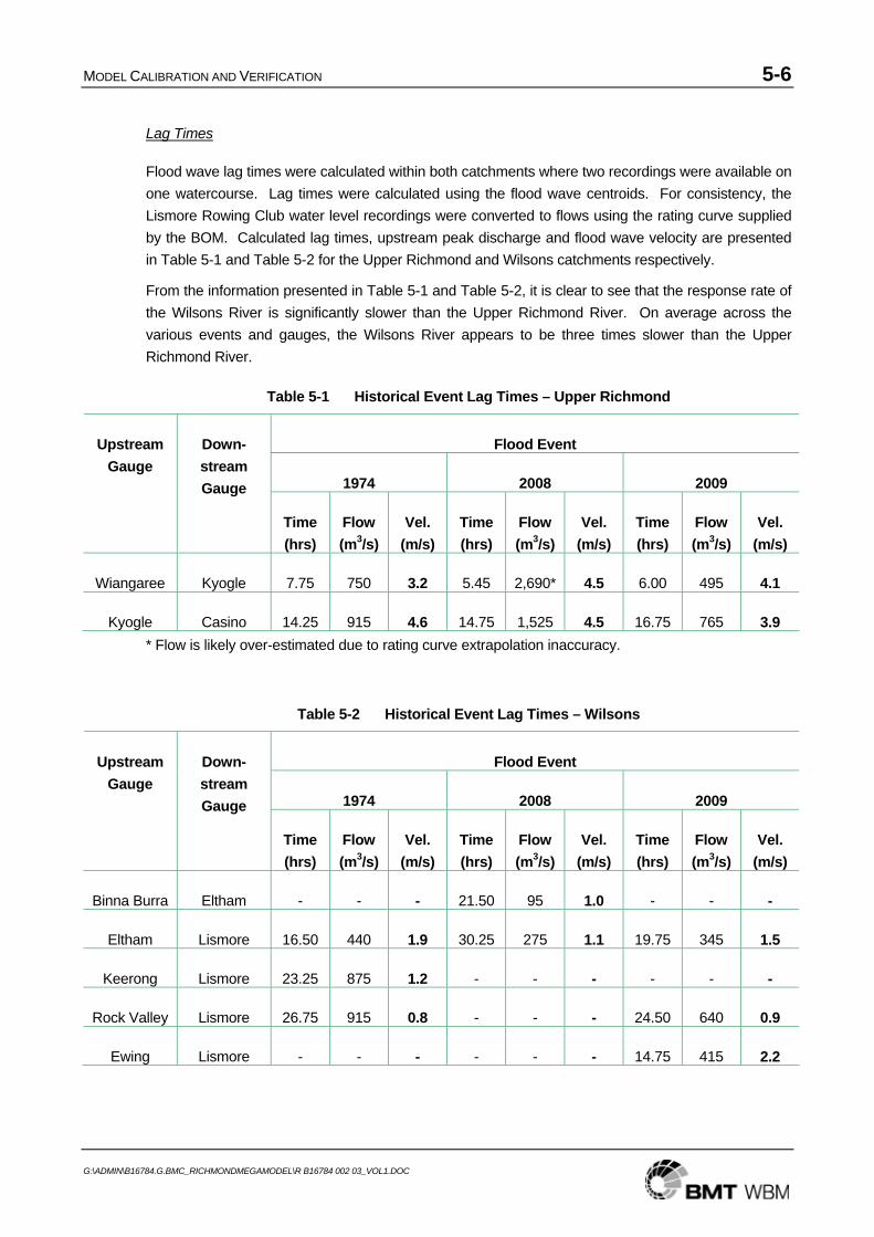
MODEL CALIBRATION AND VERIFICATION 5-6
G:\ADMIN\B16784.G.BMC_RICHMONDMEGAMODEL\R B16784 002 03_VOL1.DOC
Lag Times
Flood wave lag times were calculated within both catchments where two recordings were available on one watercourse. Lag times were calculated using the flood wave centroids. For consistency, the Lismore Rowing Club water level recordings were converted to flows using the rating curve supplied by the BOM. Calculated lag times, upstream peak discharge and flood wave velocity are presented in Table 5-1 and Table 5-2 for the Upper Richmond and Wilsons catchments respectively.
From the information presented in Table 5-1 and Table 5-2, it is clear to see that the response rate of the Wilsons River is significantly slower than the Upper Richmond River. On average across the various events and gauges, the Wilsons River appears to be three times slower than the Upper Richmond River.
Table 5-1 Historical Event Lag Times – Upper Richmond
Flood Event
1974 2008 2009
Upstream Gauge
Down-stream Gauge
Time (hrs)
Flow (m3/s)
Vel. (m/s)
Time (hrs)
Flow (m3/s)
Vel. (m/s)
Time (hrs)
Flow (m3/s)
Vel. (m/s)
Wiangaree Kyogle 7.75 750 3.2 5.45 2,690* 4.5 6.00 495 4.1
Kyogle Casino 14.25 915 4.6 14.75 1,525 4.5 16.75 765 3.9 * Flow is likely over-estimated due to rating curve extrapolation inaccuracy.
Table 5-2 Historical Event Lag Times – Wilsons
Flood Event
1974 2008 2009
Upstream Gauge
Down-stream Gauge
Time (hrs)
Flow (m3/s)
Vel. (m/s)
Time (hrs)
Flow (m3/s)
Vel. (m/s)
Time (hrs)
Flow (m3/s)
Vel. (m/s)
Binna Burra Eltham - - - 21.50 95 1.0 - - -
Eltham Lismore 16.50 440 1.9 30.25 275 1.1 19.75 345 1.5
Keerong Lismore 23.25 875 1.2 - - - - - -
Rock Valley Lismore 26.75 915 0.8 - - - 24.50 640 0.9
Ewing Lismore - - - - - - 14.75 415 2.2
MODEL CALIBRATION AND VERIFICATION 5-7
G:\ADMIN\B16784.G.BMC_RICHMONDMEGAMODEL\R B16784 002 03_VOL1.DOC
Appropriate Lag Parameters
This investigation has provided supporting evidence for use of different lag parameters for different parts of the catchment. The reason for the significant difference in response times between the two catchments is primarily due to floodplain storage. There is significant storage along the floodplains of creeks within the Wilsons catchment, often constricted by natural features, levees, roads and bridges.
Across most of the Upper Richmond, use of a catchment lag parameter (CLP) equal to 2.2 was found to provide the best calibration. Although slightly higher than the recommended average of 1.60, this value is within the range of many other calibrated catchment studies (Boyd and Bodhinayake, 2006). To represent the slower flow within the Wilsons catchment, the CLP was multiplied by 3 and applied to the lower sub-catchments and associated floodplains.
Use of CLP values of 2.2 for upper reaches and 6.6 across the floodplain areas, resulted in good agreement between the timing of the WBNM results and the corresponding stream gauges. Personal communication with the author of WBNM confirmed that the CLP of 6.6 was unusually high, although could be explained by floodplain storage and was appropriately supported by the investigation and calculations.
As a final check, the WBNM flows were compared with the flow rates at Lismore Rowing Club. Across the range of events analysed, the output from WBNM showed a good match to the recorded data.
5.5 May 2009 Event Calibration
5.5.1 Rainfall
Total rainfall was calculated for the 61 daily and pluviograph stations located across the Richmond River and surrounding catchments for the two day period commencing 09:00 20 May 2009. This time corresponds to the time of day that daily rainfall observations are recorded. Using the rainfall totals, isohyets were drawn to generate a total rainfall grid that best fit the recorded data. The resulting areal rainfall distribution is presented on Map 5-1.
The average rainfall for each sub-catchment was subsequently calculated and applied to the hydrologic model. The temporal pattern used for each sub-catchment was generally assigned based on a Thiessen distribution as shown on Map 5-2 and 5-3.
Also shown on Map 5-2 and Map 5-3 are the pluviograph recordings for each of the 20 stations used for modelling. Cumulative rainfall and percentage of total rainfall are presented in Figure 5-1 and Figure 5-2 respectively. These plots are useful for understanding the temporal pattern variation between the different pluviograph stations for a particular event. These plots were also used for establishing which temporal pattern should be assigned to a particular area.
From Figure 5-2 the southerly movement of the storm can be seen. The close grouping of the lines on Figure 5-2 also indicates a relatively consistent temporal pattern. However, there are various intense bursts within the overall event which are isolated to certain parts of the catchment.
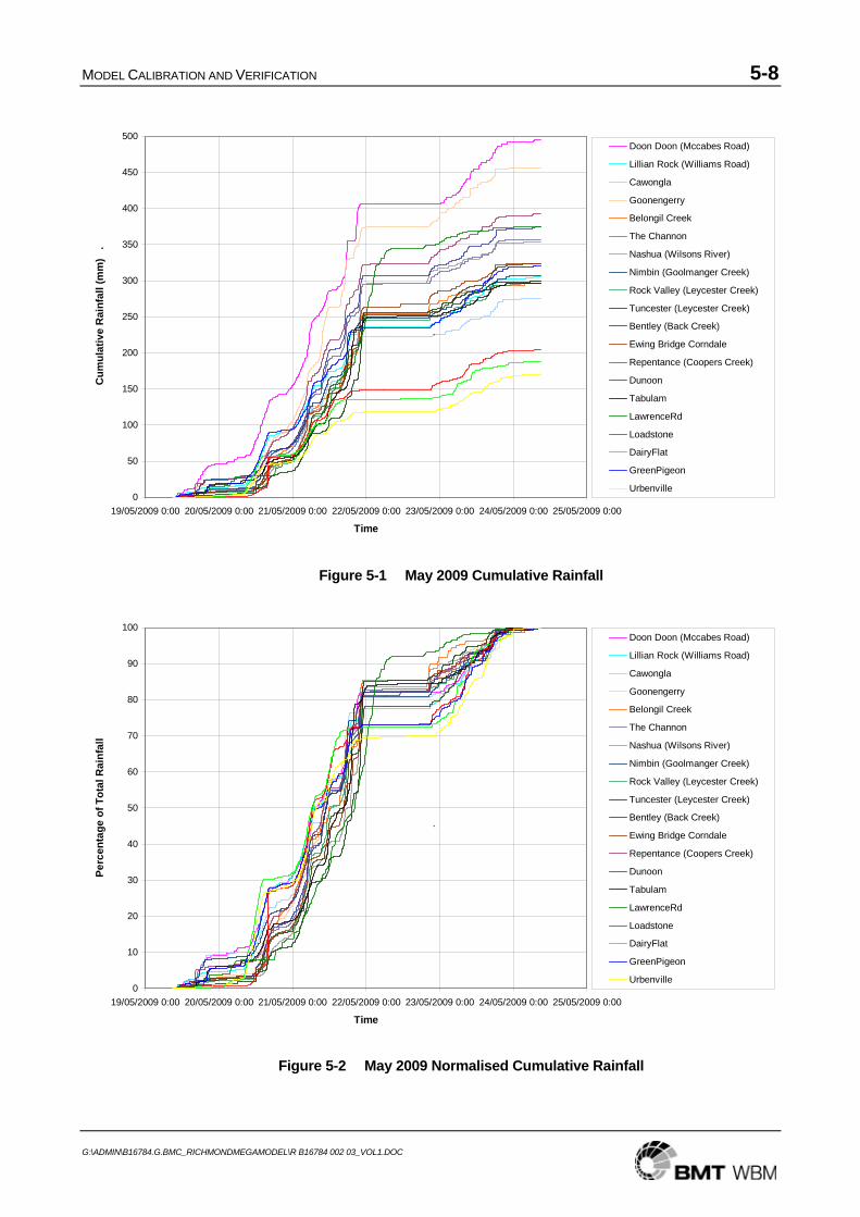
MODEL CALIBRATION AND VERIFICATION 5-8
G:\ADMIN\B16784.G.BMC_RICHMONDMEGAMODEL\R B16784 002 03_VOL1.DOC
0
50
100
150
200
250
300
350
400
450
500
19/05/2009 0:00 20/05/2009 0:00 21/05/2009 0:00 22/05/2009 0:00 23/05/2009 0:00 24/05/2009 0:00 25/05/2009 0:00
Time
Cum
ulat
ive
Rai
nfal
l (m
m)
.
Doon Doon (Mccabes Road)
Lillian Rock (Williams Road)
Cawongla
Goonengerry
Belongil Creek
The Channon
Nashua (Wilsons River)
Nimbin (Goolmanger Creek)
Rock Valley (Leycester Creek)
Tuncester (Leycester Creek)
Bentley (Back Creek)
Ewing Bridge Corndale
Repentance (Coopers Creek)
Dunoon
Tabulam
LawrenceRd
Loadstone
DairyFlat
GreenPigeon
Urbenville
`
0
10
20
30
40
50
60
70
80
90
100
19/05/2009 0:00 20/05/2009 0:00 21/05/2009 0:00 22/05/2009 0:00 23/05/2009 0:00 24/05/2009 0:00 25/05/2009 0:00
Time
Perc
enta
ge o
f Tot
al R
ainf
all
Doon Doon (Mccabes Road)
Lillian Rock (Williams Road)
Cawongla
Goonengerry
Belongil Creek
The Channon
Nashua (Wilsons River)
Nimbin (Goolmanger Creek)
Rock Valley (Leycester Creek)
Tuncester (Leycester Creek)
Bentley (Back Creek)
Ewing Bridge Corndale
Repentance (Coopers Creek)
Dunoon
Tabulam
LawrenceRd
Loadstone
DairyFlat
GreenPigeon
Urbenville
`
Figure 5-1 May 2009 Cumulative Rainfall
Figure 5-2 May 2009 Normalised Cumulative Rainfall
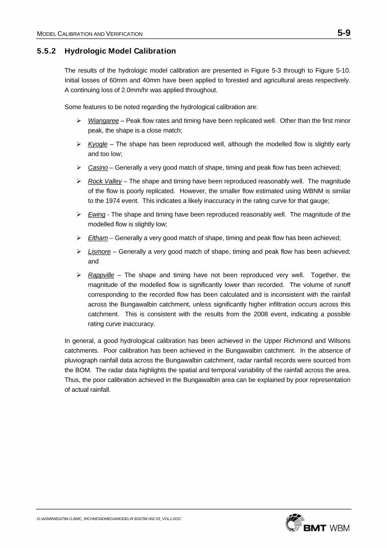
MODEL CALIBRATION AND VERIFICATION 5-9
G:\ADMIN\B16784.G.BMC_RICHMONDMEGAMODEL\R B16784 002 03_VOL1.DOC
5.5.2 Hydrologic Model Calibration
The results of the hydrologic model calibration are presented in Figure 5-3 through to Figure 5-10. Initial losses of 60mm and 40mm have been applied to forested and agricultural areas respectively. A continuing loss of 2.0mm/hr was applied throughout.
Some features to be noted regarding the hydrological calibration are:
Wiangaree – Peak flow rates and timing have been replicated well. Other than the first minor peak, the shape is a close match;
Kyogle – The shape has been reproduced well, although the modelled flow is slightly early and too low;
Casino – Generally a very good match of shape, timing and peak flow has been achieved;
Rock Valley – The shape and timing have been reproduced reasonably well. The magnitude of the flow is poorly replicated. However, the smaller flow estimated using WBNM is similar to the 1974 event. This indicates a likely inaccuracy in the rating curve for that gauge;
Ewing - The shape and timing have been reproduced reasonably well. The magnitude of the modelled flow is slightly low;
Eltham – Generally a very good match of shape, timing and peak flow has been achieved;
Lismore – Generally a very good match of shape, timing and peak flow has been achieved; and
Rappville – The shape and timing have not been reproduced very well. Together, the magnitude of the modelled flow is significantly lower than recorded. The volume of runoff corresponding to the recorded flow has been calculated and is inconsistent with the rainfall across the Bungawalbin catchment, unless significantly higher infiltration occurs across this catchment. This is consistent with the results from the 2008 event, indicating a possible rating curve inaccuracy.
In general, a good hydrological calibration has been achieved in the Upper Richmond and Wilsons catchments. Poor calibration has been achieved in the Bungawalbin catchment. In the absence of pluviograph rainfall data across the Bungawalbin catchment, radar rainfall records were sourced from the BOM. The radar data highlights the spatial and temporal variability of the rainfall across the area. Thus, the poor calibration achieved in the Bungawalbin area can be explained by poor representation of actual rainfall.
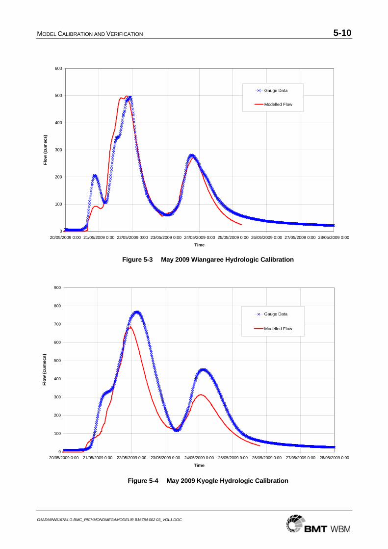
MODEL CALIBRATION AND VERIFICATION 5-10
G:\ADMIN\B16784.G.BMC_RICHMONDMEGAMODEL\R B16784 002 03_VOL1.DOC
0
100
200
300
400
500
600
20/05/2009 0:00 21/05/2009 0:00 22/05/2009 0:00 23/05/2009 0:00 24/05/2009 0:00 25/05/2009 0:00 26/05/2009 0:00 27/05/2009 0:00 28/05/2009 0:00
Time
Flow
(cum
ecs)
Gauge Data
Modelled Flow
0
100
200
300
400
500
600
700
800
900
20/05/2009 0:00 21/05/2009 0:00 22/05/2009 0:00 23/05/2009 0:00 24/05/2009 0:00 25/05/2009 0:00 26/05/2009 0:00 27/05/2009 0:00 28/05/2009 0:00
Time
Flow
(cum
ecs)
Gauge Data
Modelled Flow
Figure 5-3 May 2009 Wiangaree Hydrologic Calibration
Figure 5-4 May 2009 Kyogle Hydrologic Calibration
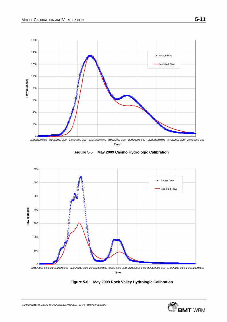
MODEL CALIBRATION AND VERIFICATION 5-11
G:\ADMIN\B16784.G.BMC_RICHMONDMEGAMODEL\R B16784 002 03_VOL1.DOC
0
200
400
600
800
1000
1200
1400
1600
20/05/2009 0:00 21/05/2009 0:00 22/05/2009 0:00 23/05/2009 0:00 24/05/2009 0:00 25/05/2009 0:00 26/05/2009 0:00 27/05/2009 0:00 28/05/2009 0:00
Time
Flow
(cum
ecs)
Gauge Data
Modelled Flow
0
100
200
300
400
500
600
700
20/05/2009 0:00 21/05/2009 0:00 22/05/2009 0:00 23/05/2009 0:00 24/05/2009 0:00 25/05/2009 0:00 26/05/2009 0:00 27/05/2009 0:00 28/05/2009 0:00
Time
Flow
(cum
ecs)
Gauge Data
Modelled Flow
Figure 5-5 May 2009 Casino Hydrologic Calibration
Figure 5-6 May 2009 Rock Valley Hydrologic Calibration
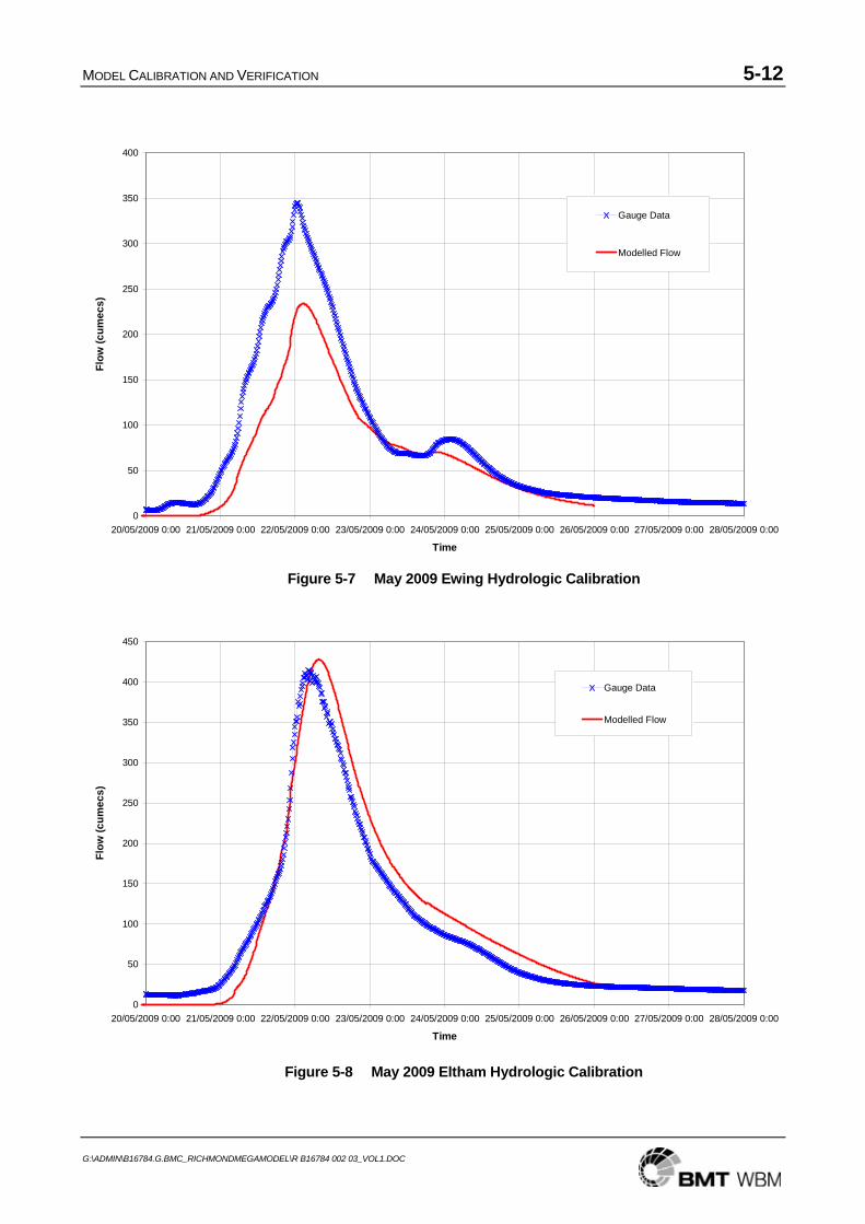
MODEL CALIBRATION AND VERIFICATION 5-12
G:\ADMIN\B16784.G.BMC_RICHMONDMEGAMODEL\R B16784 002 03_VOL1.DOC
0
50
100
150
200
250
300
350
400
20/05/2009 0:00 21/05/2009 0:00 22/05/2009 0:00 23/05/2009 0:00 24/05/2009 0:00 25/05/2009 0:00 26/05/2009 0:00 27/05/2009 0:00 28/05/2009 0:00
Time
Flow
(cum
ecs)
Gauge Data
Modelled Flow
0
50
100
150
200
250
300
350
400
450
20/05/2009 0:00 21/05/2009 0:00 22/05/2009 0:00 23/05/2009 0:00 24/05/2009 0:00 25/05/2009 0:00 26/05/2009 0:00 27/05/2009 0:00 28/05/2009 0:00
Time
Flow
(cum
ecs)
Gauge Data
Modelled Flow
Figure 5-7 May 2009 Ewing Hydrologic Calibration
Figure 5-8 May 2009 Eltham Hydrologic Calibration
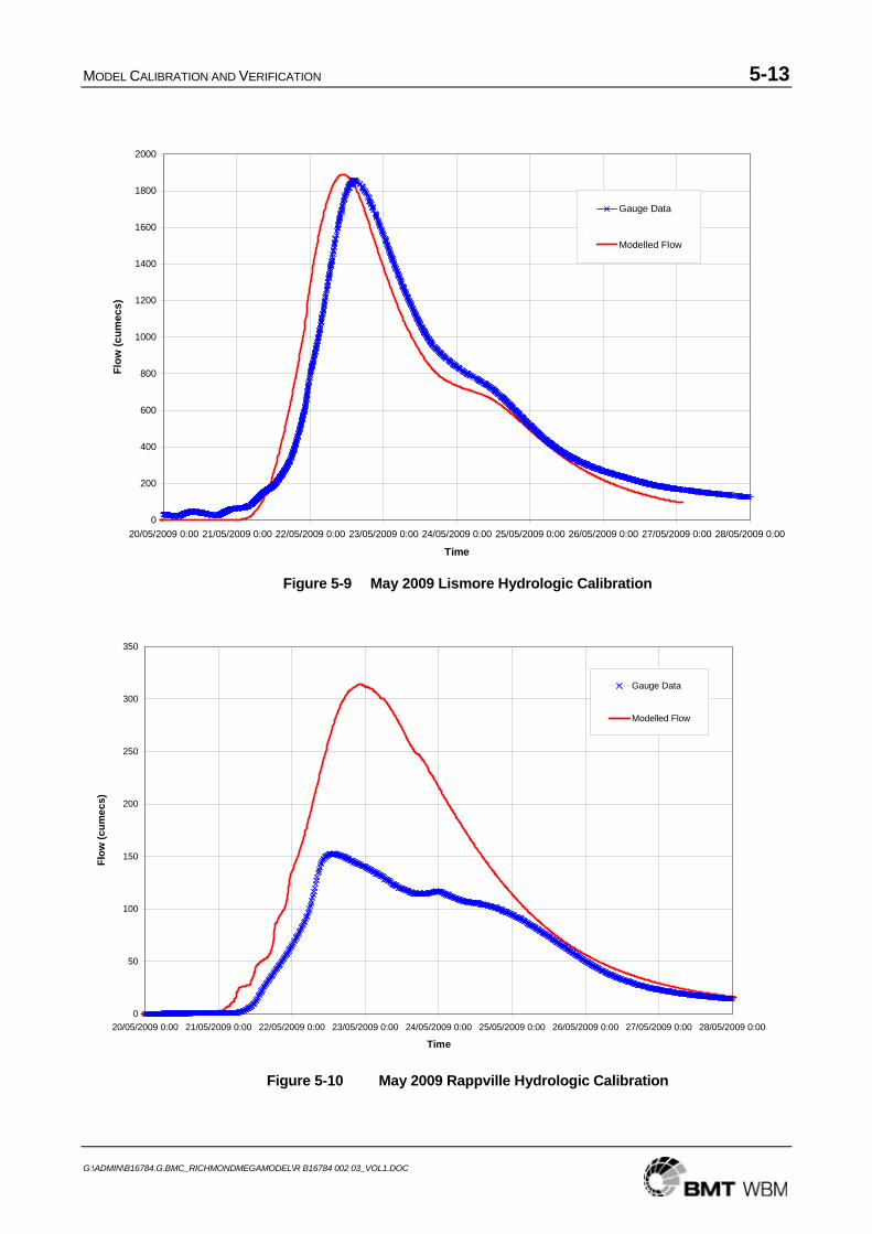
MODEL CALIBRATION AND VERIFICATION 5-13
G:\ADMIN\B16784.G.BMC_RICHMONDMEGAMODEL\R B16784 002 03_VOL1.DOC
0
200
400
600
800
1000
1200
1400
1600
1800
2000
20/05/2009 0:00 21/05/2009 0:00 22/05/2009 0:00 23/05/2009 0:00 24/05/2009 0:00 25/05/2009 0:00 26/05/2009 0:00 27/05/2009 0:00 28/05/2009 0:00
Time
Flow
(cum
ecs)
Gauge Data
Modelled Flow
0
50
100
150
200
250
300
350
20/05/2009 0:00 21/05/2009 0:00 22/05/2009 0:00 23/05/2009 0:00 24/05/2009 0:00 25/05/2009 0:00 26/05/2009 0:00 27/05/2009 0:00 28/05/2009 0:00
Time
Flow
(cum
ecs)
Gauge Data
Modelled Flow
Figure 5-9 May 2009 Lismore Hydrologic Calibration
Figure 5-10 May 2009 Rappville Hydrologic Calibration
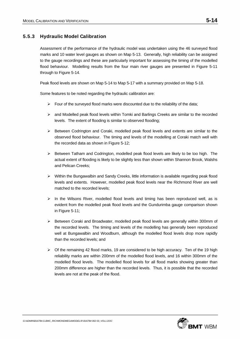
MODEL CALIBRATION AND VERIFICATION 5-14
G:\ADMIN\B16784.G.BMC_RICHMONDMEGAMODEL\R B16784 002 03_VOL1.DOC
5.5.3 Hydraulic Model Calibration
Assessment of the performance of the hydraulic model was undertaken using the 46 surveyed flood marks and 10 water level gauges as shown on Map 5-13. Generally, high reliability can be assigned to the gauge recordings and these are particularly important for assessing the timing of the modelled flood behaviour. Modelling results from the four main river gauges are presented in Figure 5-11 through to Figure 5-14.
Peak flood levels are shown on Map 5-14 to Map 5-17 with a summary provided on Map 5-18.
Some features to be noted regarding the hydraulic calibration are:
Four of the surveyed flood marks were discounted due to the reliability of the data;
and Modelled peak flood levels within Tomki and Barlings Creeks are similar to the recorded levels. The extent of flooding is similar to observed flooding;
Between Codrington and Coraki, modelled peak flood levels and extents are similar to the observed flood behaviour. The timing and levels of the modelling at Coraki match well with the recorded data as shown in Figure 5-12;
Between Tatham and Codrington, modelled peak flood levels are likely to be too high. The actual extent of flooding is likely to be slightly less than shown within Shannon Brook, Walshs and Pelican Creeks;
Within the Bungawalbin and Sandy Creeks, little information is available regarding peak flood levels and extents. However, modelled peak flood levels near the Richmond River are well matched to the recorded levels;
In the Wilsons River, modelled flood levels and timing has been reproduced well, as is evident from the modelled peak flood levels and the Gundurimba gauge comparison shown in Figure 5-11;
Between Coraki and Broadwater, modelled peak flood levels are generally within 300mm of the recorded levels. The timing and levels of the modelling has generally been reproduced well at Bungawalbin and Woodburn, although the modelled flood levels drop more rapidly than the recorded levels; and
Of the remaining 42 flood marks, 19 are considered to be high accuracy. Ten of the 19 high reliability marks are within 200mm of the modelled flood levels, and 16 within 300mm of the modelled flood levels. The modelled flood levels for all flood marks showing greater than 200mm difference are higher than the recorded levels. Thus, it is possible that the recorded levels are not at the peak of the flood.
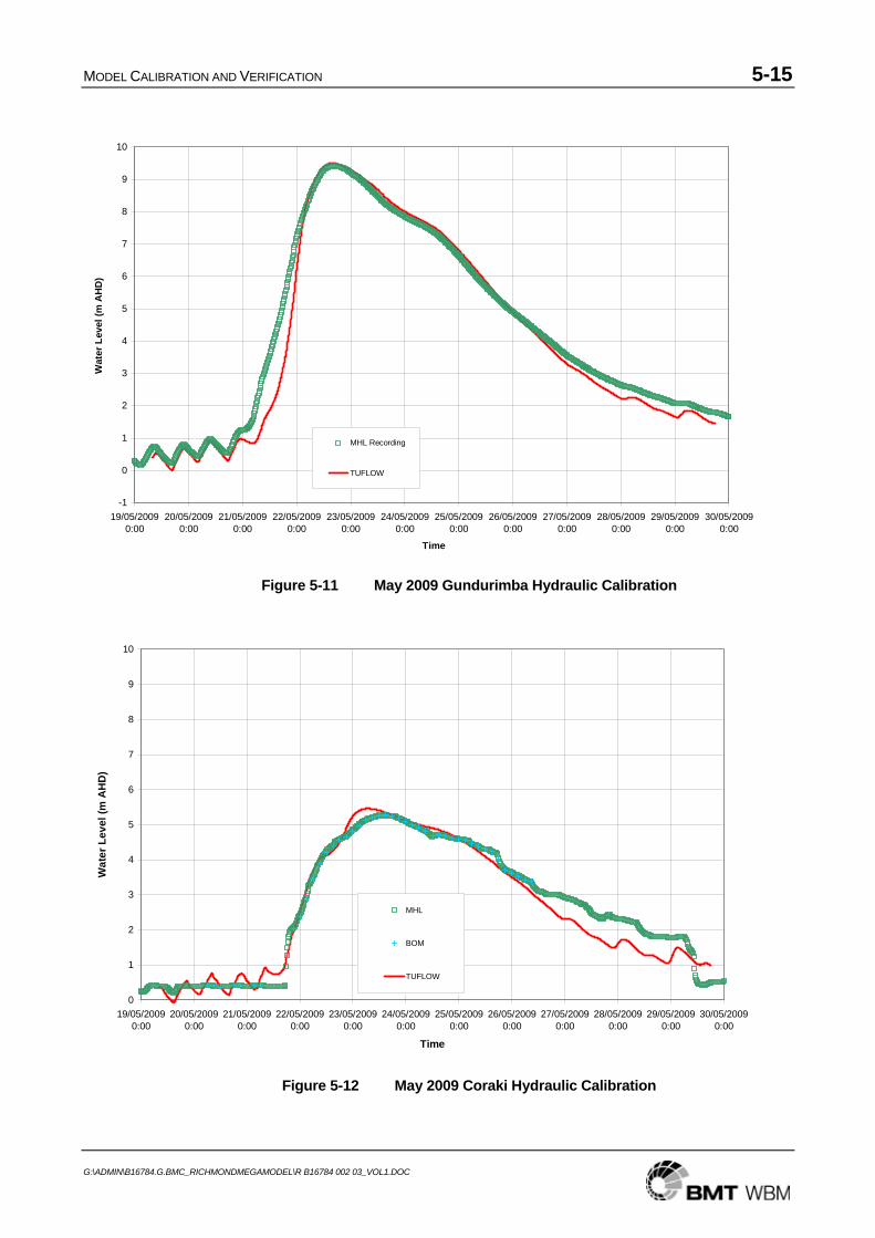
MODEL CALIBRATION AND VERIFICATION 5-15
G:\ADMIN\B16784.G.BMC_RICHMONDMEGAMODEL\R B16784 002 03_VOL1.DOC
Figure 5-11 May 2009 Gundurimba Hydraulic Calibration
Figure 5-12 May 2009 Coraki Hydraulic Calibration
-1
0
1
2
3
4
5
6
7
8
9
10
19/05/20090:00
20/05/20090:00
21/05/20090:00
22/05/20090:00
23/05/20090:00
24/05/20090:00
25/05/20090:00
26/05/20090:00
27/05/20090:00
28/05/20090:00
29/05/20090:00
30/05/20090:00
Time
Wat
er L
evel
(m A
HD
)
MHL Recording
TUFLOW
0
1
2
3
4
5
6
7
8
9
10
19/05/20090:00
20/05/20090:00
21/05/20090:00
22/05/20090:00
23/05/20090:00
24/05/20090:00
25/05/20090:00
26/05/20090:00
27/05/20090:00
28/05/20090:00
29/05/20090:00
30/05/20090:00
Time
Wat
er L
evel
(m A
HD
)
MHL
BOM
TUFLOW
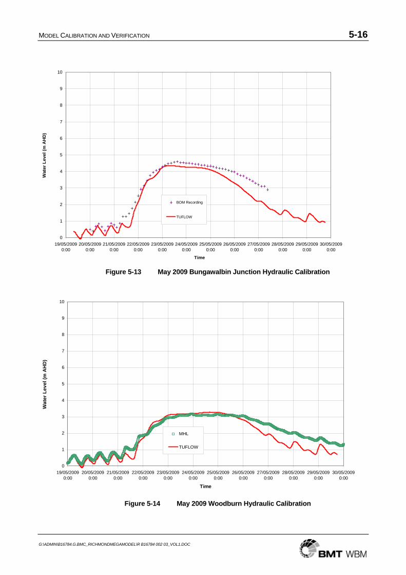
MODEL CALIBRATION AND VERIFICATION 5-16
G:\ADMIN\B16784.G.BMC_RICHMONDMEGAMODEL\R B16784 002 03_VOL1.DOC
Figure 5-13 May 2009 Bungawalbin Junction Hydraulic Calibration
Figure 5-14 May 2009 Woodburn Hydraulic Calibration
0
1
2
3
4
5
6
7
8
9
10
19/05/20090:00
20/05/20090:00
21/05/20090:00
22/05/20090:00
23/05/20090:00
24/05/20090:00
25/05/20090:00
26/05/20090:00
27/05/20090:00
28/05/20090:00
29/05/20090:00
30/05/20090:00
Time
Wat
er L
evel
(m A
HD
)
BOM Recording
TUFLOW
0
1
2
3
4
5
6
7
8
9
10
19/05/20090:00
20/05/20090:00
21/05/20090:00
22/05/20090:00
23/05/20090:00
24/05/20090:00
25/05/20090:00
26/05/20090:00
27/05/20090:00
28/05/20090:00
29/05/20090:00
30/05/20090:00
Time
Wat
er L
evel
(m A
HD
)
MHL
TUFLOW
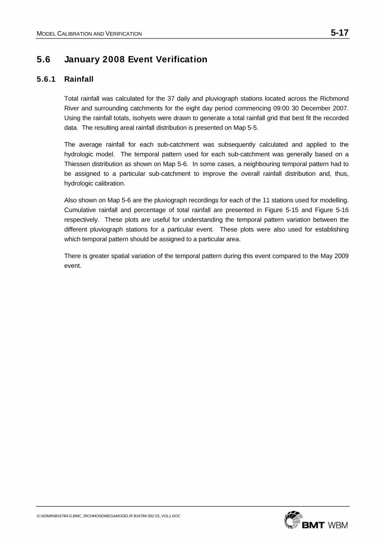
MODEL CALIBRATION AND VERIFICATION 5-17
G:\ADMIN\B16784.G.BMC_RICHMONDMEGAMODEL\R B16784 002 03_VOL1.DOC
5.6 January 2008 Event Verification
5.6.1 Rainfall
Total rainfall was calculated for the 37 daily and pluviograph stations located across the Richmond River and surrounding catchments for the eight day period commencing 09:00 30 December 2007. Using the rainfall totals, isohyets were drawn to generate a total rainfall grid that best fit the recorded data. The resulting areal rainfall distribution is presented on Map 5-5.
The average rainfall for each sub-catchment was subsequently calculated and applied to the hydrologic model. The temporal pattern used for each sub-catchment was generally based on a Thiessen distribution as shown on Map 5-6. In some cases, a neighbouring temporal pattern had to be assigned to a particular sub-catchment to improve the overall rainfall distribution and, thus, hydrologic calibration.
Also shown on Map 5-6 are the pluviograph recordings for each of the 11 stations used for modelling. Cumulative rainfall and percentage of total rainfall are presented in Figure 5-15 and Figure 5-16 respectively. These plots are useful for understanding the temporal pattern variation between the different pluviograph stations for a particular event. These plots were also used for establishing which temporal pattern should be assigned to a particular area.
There is greater spatial variation of the temporal pattern during this event compared to the May 2009 event.
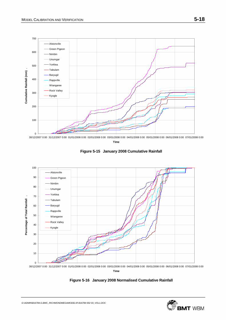
MODEL CALIBRATION AND VERIFICATION 5-18
G:\ADMIN\B16784.G.BMC_RICHMONDMEGAMODEL\R B16784 002 03_VOL1.DOC
0
100
200
300
400
500
600
700
30/12/2007 0:00 31/12/2007 0:00 01/01/2008 0:00 02/01/2008 0:00 03/01/2008 0:00 04/01/2008 0:00 05/01/2008 0:00 06/01/2008 0:00 07/01/2008 0:00
Time
Cum
ulat
ive
Rai
nfal
l (m
m)
.
Alstonville
Green Pigeon
Nimbin
Unumgar
Yorklea
Tabulam
Baryugil
Rappville
Wiangaree
Rock Valley
Kyogle
0
10
20
30
40
50
60
70
80
90
100
30/12/2007 0:00 31/12/2007 0:00 01/01/2008 0:00 02/01/2008 0:00 03/01/2008 0:00 04/01/2008 0:00 05/01/2008 0:00 06/01/2008 0:00 07/01/2008 0:00
Time
Perc
enta
ge o
f Tot
al R
ainf
all
.
Alstonville
Green Pigeon
Nimbin
Unumgar
Yorklea
Tabulam
Baryugil
Rappville
Wiangaree
Rock Valley
Kyogle
Figure 5-15 January 2008 Cumulative Rainfall
Figure 5-16 January 2008 Normalised Cumulative Rainfall
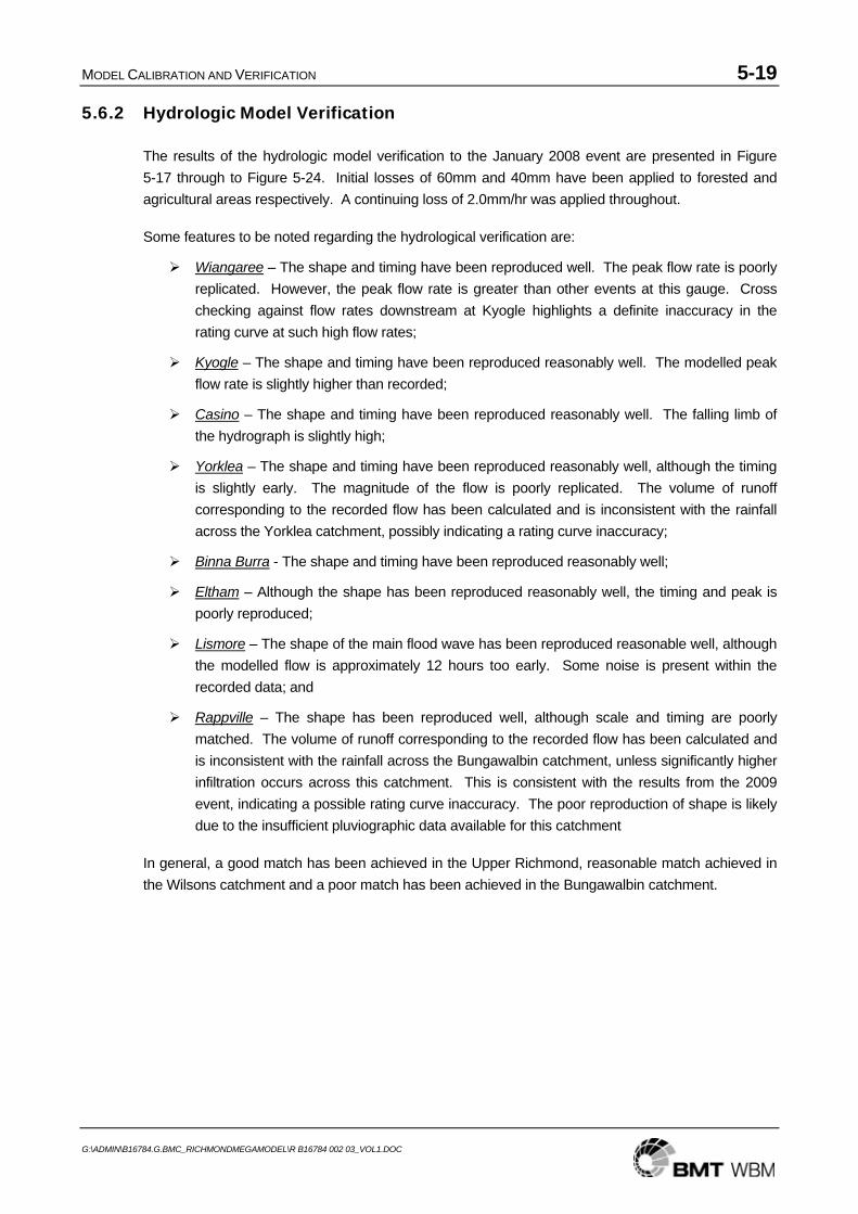
MODEL CALIBRATION AND VERIFICATION 5-19
G:\ADMIN\B16784.G.BMC_RICHMONDMEGAMODEL\R B16784 002 03_VOL1.DOC
5.6.2 Hydrologic Model Verification
The results of the hydrologic model verification to the January 2008 event are presented in Figure 5-17 through to Figure 5-24. Initial losses of 60mm and 40mm have been applied to forested and agricultural areas respectively. A continuing loss of 2.0mm/hr was applied throughout.
Some features to be noted regarding the hydrological verification are:
Wiangaree – The shape and timing have been reproduced well. The peak flow rate is poorly replicated. However, the peak flow rate is greater than other events at this gauge. Cross checking against flow rates downstream at Kyogle highlights a definite inaccuracy in the rating curve at such high flow rates;
Kyogle – The shape and timing have been reproduced reasonably well. The modelled peak flow rate is slightly higher than recorded;
Casino – The shape and timing have been reproduced reasonably well. The falling limb of the hydrograph is slightly high;
Yorklea – The shape and timing have been reproduced reasonably well, although the timing is slightly early. The magnitude of the flow is poorly replicated. The volume of runoff corresponding to the recorded flow has been calculated and is inconsistent with the rainfall across the Yorklea catchment, possibly indicating a rating curve inaccuracy;
Binna Burra - The shape and timing have been reproduced reasonably well;
Eltham – Although the shape has been reproduced reasonably well, the timing and peak is poorly reproduced;
Lismore – The shape of the main flood wave has been reproduced reasonable well, although the modelled flow is approximately 12 hours too early. Some noise is present within the recorded data; and
Rappville – The shape has been reproduced well, although scale and timing are poorly matched. The volume of runoff corresponding to the recorded flow has been calculated and is inconsistent with the rainfall across the Bungawalbin catchment, unless significantly higher infiltration occurs across this catchment. This is consistent with the results from the 2009 event, indicating a possible rating curve inaccuracy. The poor reproduction of shape is likely due to the insufficient pluviographic data available for this catchment
In general, a good match has been achieved in the Upper Richmond, reasonable match achieved in the Wilsons catchment and a poor match has been achieved in the Bungawalbin catchment.
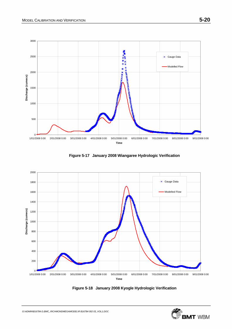
MODEL CALIBRATION AND VERIFICATION 5-20
G:\ADMIN\B16784.G.BMC_RICHMONDMEGAMODEL\R B16784 002 03_VOL1.DOC
0
500
1000
1500
2000
2500
3000
1/01/2008 0:00 2/01/2008 0:00 3/01/2008 0:00 4/01/2008 0:00 5/01/2008 0:00 6/01/2008 0:00 7/01/2008 0:00 8/01/2008 0:00 9/01/2008 0:00
Time
Dis
char
ge (c
umec
s)
Gauge Data
Modelled Flow
0
200
400
600
800
1000
1200
1400
1600
1800
2000
1/01/2008 0:00 2/01/2008 0:00 3/01/2008 0:00 4/01/2008 0:00 5/01/2008 0:00 6/01/2008 0:00 7/01/2008 0:00 8/01/2008 0:00 9/01/2008 0:00
Time
Dis
char
ge (c
umec
s)
Gauge Data
Modelled Flow
Figure 5-17 January 2008 Wiangaree Hydrologic Verification
Figure 5-18 January 2008 Kyogle Hydrologic Verification
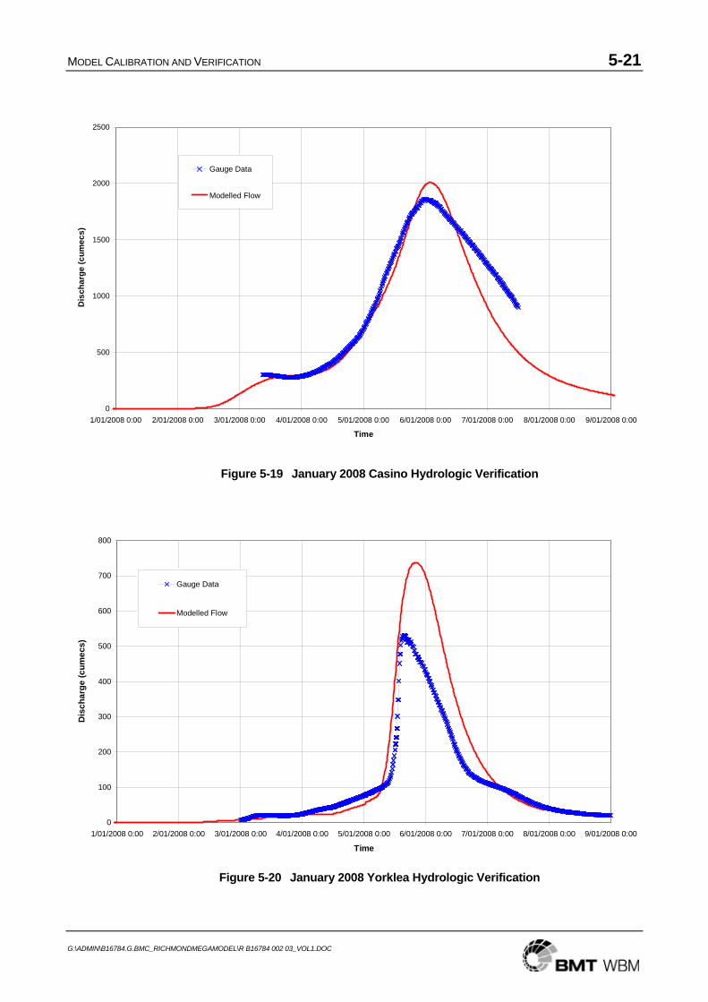
MODEL CALIBRATION AND VERIFICATION 5-21
G:\ADMIN\B16784.G.BMC_RICHMONDMEGAMODEL\R B16784 002 03_VOL1.DOC
0
500
1000
1500
2000
2500
1/01/2008 0:00 2/01/2008 0:00 3/01/2008 0:00 4/01/2008 0:00 5/01/2008 0:00 6/01/2008 0:00 7/01/2008 0:00 8/01/2008 0:00 9/01/2008 0:00
Time
Dis
char
ge (c
umec
s)
Gauge Data
Modelled Flow
0
100
200
300
400
500
600
700
800
1/01/2008 0:00 2/01/2008 0:00 3/01/2008 0:00 4/01/2008 0:00 5/01/2008 0:00 6/01/2008 0:00 7/01/2008 0:00 8/01/2008 0:00 9/01/2008 0:00
Time
Dis
char
ge (c
umec
s)
Gauge Data
Modelled Flow
Figure 5-19 January 2008 Casino Hydrologic Verification
Figure 5-20 January 2008 Yorklea Hydrologic Verification
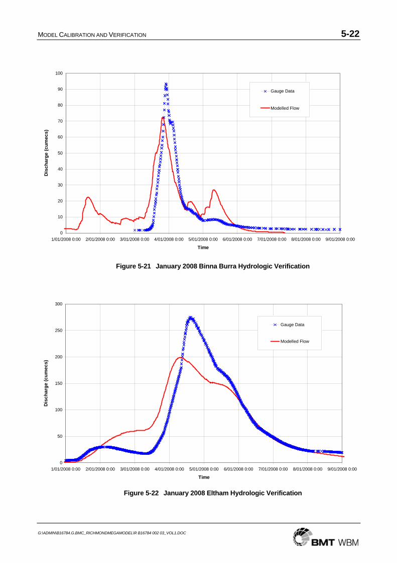
MODEL CALIBRATION AND VERIFICATION 5-22
G:\ADMIN\B16784.G.BMC_RICHMONDMEGAMODEL\R B16784 002 03_VOL1.DOC
0
10
20
30
40
50
60
70
80
90
100
1/01/2008 0:00 2/01/2008 0:00 3/01/2008 0:00 4/01/2008 0:00 5/01/2008 0:00 6/01/2008 0:00 7/01/2008 0:00 8/01/2008 0:00 9/01/2008 0:00
Time
Dis
char
ge (c
umec
s)
Gauge Data
Modelled Flow
0
50
100
150
200
250
300
1/01/2008 0:00 2/01/2008 0:00 3/01/2008 0:00 4/01/2008 0:00 5/01/2008 0:00 6/01/2008 0:00 7/01/2008 0:00 8/01/2008 0:00 9/01/2008 0:00
Time
Dis
char
ge (c
umec
s)
Gauge Data
Modelled Flow
Figure 5-21 January 2008 Binna Burra Hydrologic Verification
Figure 5-22 January 2008 Eltham Hydrologic Verification
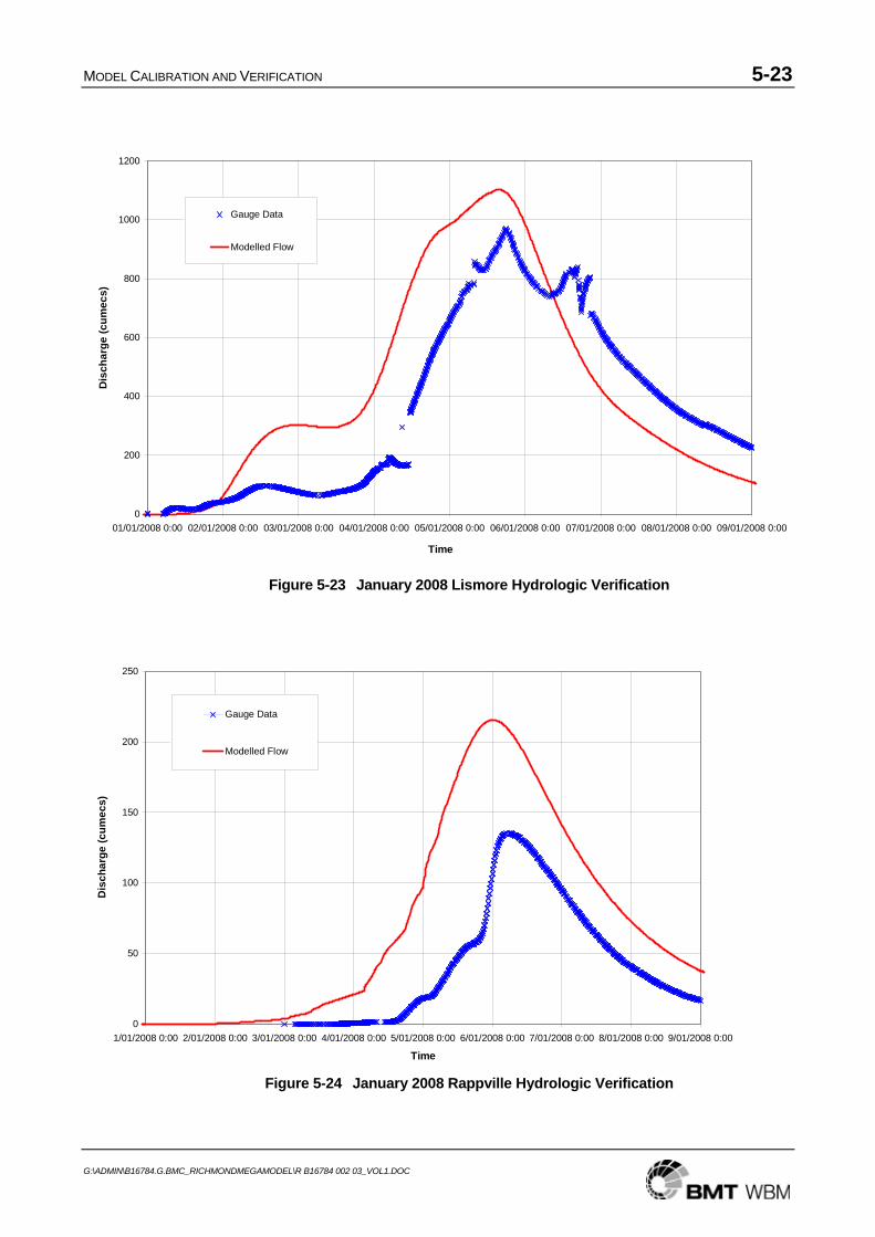
MODEL CALIBRATION AND VERIFICATION 5-23
G:\ADMIN\B16784.G.BMC_RICHMONDMEGAMODEL\R B16784 002 03_VOL1.DOC
0
200
400
600
800
1000
1200
01/01/2008 0:00 02/01/2008 0:00 03/01/2008 0:00 04/01/2008 0:00 05/01/2008 0:00 06/01/2008 0:00 07/01/2008 0:00 08/01/2008 0:00 09/01/2008 0:00
Time
Dis
char
ge (c
umec
s)
Gauge Data
Modelled Flow
0
50
100
150
200
250
1/01/2008 0:00 2/01/2008 0:00 3/01/2008 0:00 4/01/2008 0:00 5/01/2008 0:00 6/01/2008 0:00 7/01/2008 0:00 8/01/2008 0:00 9/01/2008 0:00
Time
Dis
char
ge (c
umec
s)
Gauge Data
Modelled Flow
Figure 5-23 January 2008 Lismore Hydrologic Verification
Figure 5-24 January 2008 Rappville Hydrologic Verification
MODEL CALIBRATION AND VERIFICATION 5-24
G:\ADMIN\B16784.G.BMC_RICHMONDMEGAMODEL\R B16784 002 03_VOL1.DOC
5.6.3 Hydraulic Model Verification
Hydraulic model verification for this event was undertaken using 78 surveyed flood marks and ten water level gauges as shown on Map 5-19. Modelling results for five of the main river gauges are presented in Figure 5-25 through to Figure 5-29.
Peak flood levels are shown on Map 5-20 to Map 5-23 with a summary provided on Map 5-24.
Some features to be noted regarding the hydraulic verification are:
Fifteen of the surveyed flood marks were discounted due to the reliability of the data;
Modelled peak flood levels between Casino and Tatham are generally lower than the recorded levels;
Between Tatham and Coraki there is significant variability between modelled and recorded peak flood levels;
At Coraki, the gauge stopped recording soon after midnight on the 4 January 2008. The recorded flood levels and timing prior to the gauge failure show a good match as shown in Figure 5-26, although some deviation is shown immediately prior to failure. The gauge restarted recording four days later on the 9 January 2008. However, the recorded and modelled flood levels show significant discrepancy. On Map 5-24, the peak flood levels appear to be too low around the Coraki area. Further refinement of this area will be undertaken prior to issue of the final report;
The timing and peak flood levels at Bungawalbin Junction differ from the recorded data. Further refinement of this area will be undertaken prior to issue of the final report;
Within the lower Bungawalbin, there is variability between the numerous recorded flood levels, in an area where the flood surface is relatively flat. However, the general trend is that the modelled peak flood levels appear to be too low; and
Between Bungawalbin Junction and Broadwater, peak flood levels have been reproduced relatively well, although there appears to be some outliers in the recorded data.
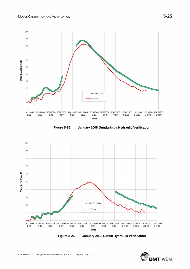
MODEL CALIBRATION AND VERIFICATION 5-25
G:\ADMIN\B16784.G.BMC_RICHMONDMEGAMODEL\R B16784 002 03_VOL1.DOC
-1
0
1
2
3
4
5
6
7
8
9
10
1/01/20080:00
2/01/20080:00
3/01/20080:00
4/01/20080:00
5/01/20080:00
6/01/20080:00
7/01/20080:00
8/01/20080:00
9/01/20080:00
10/01/2008 0:00
11/01/2008 0:00
12/01/2008 0:00
13/01/2008 0:00
Time
Wat
er L
evel
(m A
HD
)
MHL Recording
TUFLOW
0
1
2
3
4
5
6
7
8
9
10
1/01/20080:00
2/01/20080:00
3/01/20080:00
4/01/20080:00
5/01/20080:00
6/01/20080:00
7/01/20080:00
8/01/20080:00
9/01/20080:00
10/01/2008 0:00
11/01/2008 0:00
12/01/2008 0:00
13/01/2008 0:00
Time
Wat
er L
evel
(m A
HD
)
MHL Recording
TUFLOW
Figure 5-25 January 2008 Gundurimba Hydraulic Verification
Figure 5-26 January 2008 Coraki Hydraulic Verification
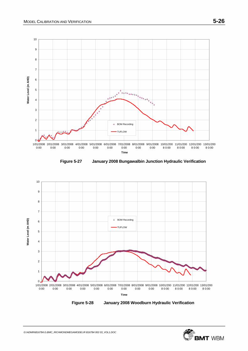
MODEL CALIBRATION AND VERIFICATION 5-26
G:\ADMIN\B16784.G.BMC_RICHMONDMEGAMODEL\R B16784 002 03_VOL1.DOC
Figure 5-27 January 2008 Bungawalbin Junction Hydraulic Verification
Figure 5-28 January 2008 Woodburn Hydraulic Verification
0
1
2
3
4
5
6
7
8
9
10
1/01/20080:00
2/01/20080:00
3/01/20080:00
4/01/20080:00
5/01/20080:00
6/01/20080:00
7/01/20080:00
8/01/20080:00
9/01/20080:00
10/01/2008 0:00
11/01/2008 0:00
12/01/2008 0:00
13/01/2008 0:00
Time
Wat
er L
evel
(m A
HD
)
BOM Recording
TUFLOW
0
1
2
3
4
5
6
7
8
9
10
1/01/20080:00
2/01/20080:00
3/01/20080:00
4/01/20080:00
5/01/20080:00
6/01/20080:00
7/01/20080:00
8/01/20080:00
9/01/20080:00
10/01/2008 0:00
11/01/2008 0:00
12/01/2008 0:00
13/01/2008 0:00
Time
Wat
er L
evel
(m A
HD
)
BOM Recording
TUFLOW
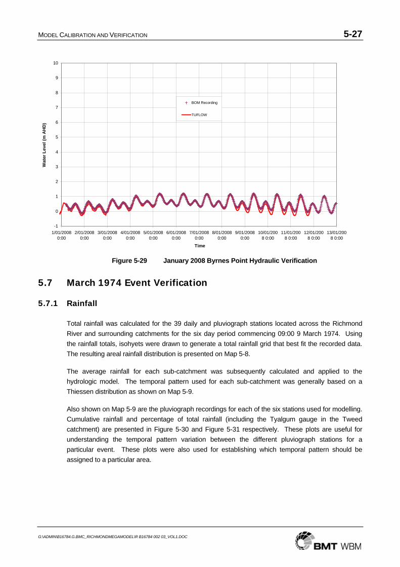
MODEL CALIBRATION AND VERIFICATION 5-27
G:\ADMIN\B16784.G.BMC_RICHMONDMEGAMODEL\R B16784 002 03_VOL1.DOC
Figure 5-29 January 2008 Byrnes Point Hydraulic Verification
5.7 March 1974 Event Verification
5.7.1 Rainfall
Total rainfall was calculated for the 39 daily and pluviograph stations located across the Richmond River and surrounding catchments for the six day period commencing 09:00 9 March 1974. Using the rainfall totals, isohyets were drawn to generate a total rainfall grid that best fit the recorded data. The resulting areal rainfall distribution is presented on Map 5-8.
The average rainfall for each sub-catchment was subsequently calculated and applied to the hydrologic model. The temporal pattern used for each sub-catchment was generally based on a Thiessen distribution as shown on Map 5-9.
Also shown on Map 5-9 are the pluviograph recordings for each of the six stations used for modelling. Cumulative rainfall and percentage of total rainfall (including the Tyalgum gauge in the Tweed catchment) are presented in Figure 5-30 and Figure 5-31 respectively. These plots are useful for understanding the temporal pattern variation between the different pluviograph stations for a particular event. These plots were also used for establishing which temporal pattern should be assigned to a particular area.
-1
0
1
2
3
4
5
6
7
8
9
10
1/01/20080:00
2/01/20080:00
3/01/20080:00
4/01/20080:00
5/01/20080:00
6/01/20080:00
7/01/20080:00
8/01/20080:00
9/01/20080:00
10/01/2008 0:00
11/01/2008 0:00
12/01/2008 0:00
13/01/2008 0:00
Time
Wat
er L
evel
(m A
HD
)
BOM Recording
TUFLOW
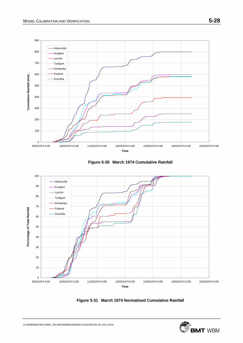
MODEL CALIBRATION AND VERIFICATION 5-28
G:\ADMIN\B16784.G.BMC_RICHMONDMEGAMODEL\R B16784 002 03_VOL1.DOC
0
100
200
300
400
500
600
700
800
900
9/03/1974 0:00 10/03/1974 0:00 11/03/1974 0:00 12/03/1974 0:00 13/03/1974 0:00 14/03/1974 0:00 15/03/1974 0:00
Time
Cum
ulat
ive
Rai
nfal
l (m
m)
.
Alstonville
Kunghur
Lynchs
Tyalgum
Kimberley
Federal
Grevillia
0
10
20
30
40
50
60
70
80
90
100
9/03/1974 0:00 10/03/1974 0:00 11/03/1974 0:00 12/03/1974 0:00 13/03/1974 0:00 14/03/1974 0:00 15/03/1974 0:00
Time
Perc
enta
ge o
f Tot
al R
ainf
all
Alstonville
Kunghur
Lynchs
Tyalgum
Kimberley
Federal
Grevillia
Figure 5-30 March 1974 Cumulative Rainfall
Figure 5-31 March 1974 Normalised Cumulative Rainfall
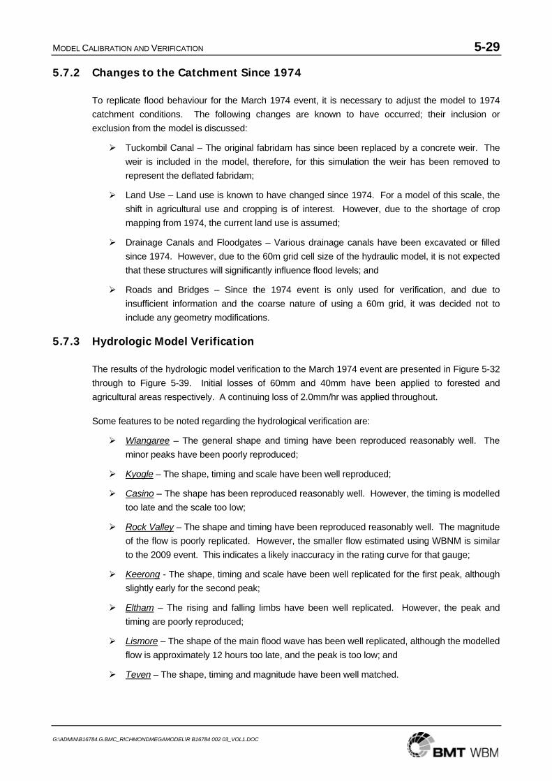
MODEL CALIBRATION AND VERIFICATION 5-29
G:\ADMIN\B16784.G.BMC_RICHMONDMEGAMODEL\R B16784 002 03_VOL1.DOC
5.7.2 Changes to the Catchment Since 1974
To replicate flood behaviour for the March 1974 event, it is necessary to adjust the model to 1974 catchment conditions. The following changes are known to have occurred; their inclusion or exclusion from the model is discussed:
Tuckombil Canal – The original fabridam has since been replaced by a concrete weir. The weir is included in the model, therefore, for this simulation the weir has been removed to represent the deflated fabridam;
Land Use – Land use is known to have changed since 1974. For a model of this scale, the shift in agricultural use and cropping is of interest. However, due to the shortage of crop mapping from 1974, the current land use is assumed;
Drainage Canals and Floodgates – Various drainage canals have been excavated or filled since 1974. However, due to the 60m grid cell size of the hydraulic model, it is not expected that these structures will significantly influence flood levels; and
Roads and Bridges – Since the 1974 event is only used for verification, and due to insufficient information and the coarse nature of using a 60m grid, it was decided not to include any geometry modifications.
5.7.3 Hydrologic Model Verification
The results of the hydrologic model verification to the March 1974 event are presented in Figure 5-32 through to Figure 5-39. Initial losses of 60mm and 40mm have been applied to forested and agricultural areas respectively. A continuing loss of 2.0mm/hr was applied throughout.
Some features to be noted regarding the hydrological verification are:
Wiangaree – The general shape and timing have been reproduced reasonably well. The minor peaks have been poorly reproduced;
Kyogle – The shape, timing and scale have been well reproduced;
Casino – The shape has been reproduced reasonably well. However, the timing is modelled too late and the scale too low;
Rock Valley – The shape and timing have been reproduced reasonably well. The magnitude of the flow is poorly replicated. However, the smaller flow estimated using WBNM is similar to the 2009 event. This indicates a likely inaccuracy in the rating curve for that gauge;
Keerong - The shape, timing and scale have been well replicated for the first peak, although slightly early for the second peak;
Eltham – The rising and falling limbs have been well replicated. However, the peak and timing are poorly reproduced;
Lismore – The shape of the main flood wave has been well replicated, although the modelled flow is approximately 12 hours too late, and the peak is too low; and
Teven – The shape, timing and magnitude have been well matched.
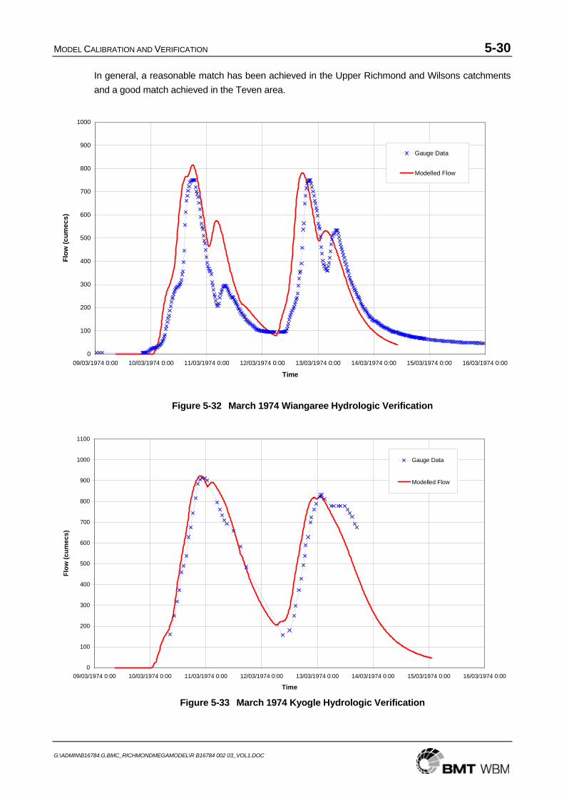
MODEL CALIBRATION AND VERIFICATION 5-30
G:\ADMIN\B16784.G.BMC_RICHMONDMEGAMODEL\R B16784 002 03_VOL1.DOC
0
100
200
300
400
500
600
700
800
900
1000
09/03/1974 0:00 10/03/1974 0:00 11/03/1974 0:00 12/03/1974 0:00 13/03/1974 0:00 14/03/1974 0:00 15/03/1974 0:00 16/03/1974 0:00
Time
Flow
(cum
ecs)
Gauge Data
Modelled Flow
0
100
200
300
400
500
600
700
800
900
1000
1100
09/03/1974 0:00 10/03/1974 0:00 11/03/1974 0:00 12/03/1974 0:00 13/03/1974 0:00 14/03/1974 0:00 15/03/1974 0:00 16/03/1974 0:00
Time
Flow
(cum
ecs)
Gauge Data
Modelled Flow
In general, a reasonable match has been achieved in the Upper Richmond and Wilsons catchments and a good match achieved in the Teven area.
Figure 5-32 March 1974 Wiangaree Hydrologic Verification
Figure 5-33 March 1974 Kyogle Hydrologic Verification
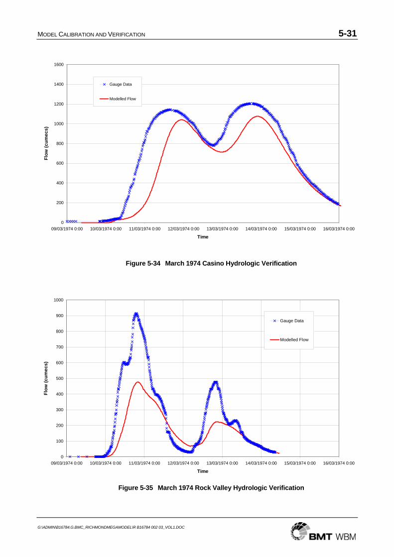
MODEL CALIBRATION AND VERIFICATION 5-31
G:\ADMIN\B16784.G.BMC_RICHMONDMEGAMODEL\R B16784 002 03_VOL1.DOC
0
200
400
600
800
1000
1200
1400
1600
09/03/1974 0:00 10/03/1974 0:00 11/03/1974 0:00 12/03/1974 0:00 13/03/1974 0:00 14/03/1974 0:00 15/03/1974 0:00 16/03/1974 0:00
Time
Flow
(cum
ecs)
Gauge Data
Modelled Flow
0
100
200
300
400
500
600
700
800
900
1000
09/03/1974 0:00 10/03/1974 0:00 11/03/1974 0:00 12/03/1974 0:00 13/03/1974 0:00 14/03/1974 0:00 15/03/1974 0:00 16/03/1974 0:00
Time
Flow
(cum
ecs)
Gauge Data
Modelled Flow
Figure 5-34 March 1974 Casino Hydrologic Verification
Figure 5-35 March 1974 Rock Valley Hydrologic Verification
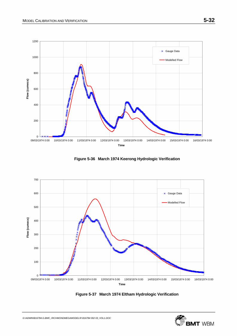
MODEL CALIBRATION AND VERIFICATION 5-32
G:\ADMIN\B16784.G.BMC_RICHMONDMEGAMODEL\R B16784 002 03_VOL1.DOC
0
200
400
600
800
1000
1200
09/03/1974 0:00 10/03/1974 0:00 11/03/1974 0:00 12/03/1974 0:00 13/03/1974 0:00 14/03/1974 0:00 15/03/1974 0:00 16/03/1974 0:00
Time
Flow
(cum
ecs)
Gauge Data
Modelled Flow
0
100
200
300
400
500
600
700
09/03/1974 0:00 10/03/1974 0:00 11/03/1974 0:00 12/03/1974 0:00 13/03/1974 0:00 14/03/1974 0:00 15/03/1974 0:00 16/03/1974 0:00
Time
Flow
(cum
ecs)
Gauge Data
Modelled Flow
Figure 5-36 March 1974 Keerong Hydrologic Verification
Figure 5-37 March 1974 Eltham Hydrologic Verification
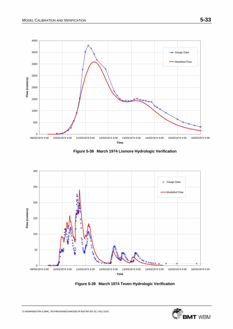
MODEL CALIBRATION AND VERIFICATION 5-33
G:\ADMIN\B16784.G.BMC_RICHMONDMEGAMODEL\R B16784 002 03_VOL1.DOC
0
500
1000
1500
2000
2500
3000
3500
4000
09/03/1974 0:00 10/03/1974 0:00 11/03/1974 0:00 12/03/1974 0:00 13/03/1974 0:00 14/03/1974 0:00 15/03/1974 0:00 16/03/1974 0:00
Time
Flow
(cum
ecs)
Gauge Data
Modelled Flow
0
50
100
150
200
250
300
09/03/1974 0:00 10/03/1974 0:00 11/03/1974 0:00 12/03/1974 0:00 13/03/1974 0:00 14/03/1974 0:00 15/03/1974 0:00 16/03/1974 0:00
Time
Flow
(cum
ecs)
Gauge Data
Modelled Flow
Figure 5-38 March 1974 Lismore Hydrologic Verification
Figure 5-39 March 1974 Teven Hydrologic Verification
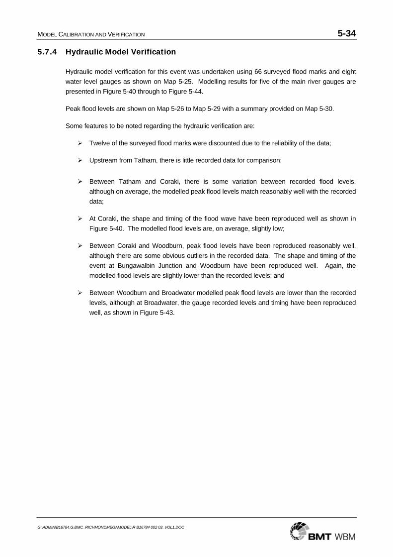
MODEL CALIBRATION AND VERIFICATION 5-34
G:\ADMIN\B16784.G.BMC_RICHMONDMEGAMODEL\R B16784 002 03_VOL1.DOC
5.7.4 Hydraulic Model Verification
Hydraulic model verification for this event was undertaken using 66 surveyed flood marks and eight water level gauges as shown on Map 5-25. Modelling results for five of the main river gauges are presented in Figure 5-40 through to Figure 5-44.
Peak flood levels are shown on Map 5-26 to Map 5-29 with a summary provided on Map 5-30.
Some features to be noted regarding the hydraulic verification are:
Twelve of the surveyed flood marks were discounted due to the reliability of the data;
Upstream from Tatham, there is little recorded data for comparison;
Between Tatham and Coraki, there is some variation between recorded flood levels, although on average, the modelled peak flood levels match reasonably well with the recorded data;
At Coraki, the shape and timing of the flood wave have been reproduced well as shown in Figure 5-40. The modelled flood levels are, on average, slightly low;
Between Coraki and Woodburn, peak flood levels have been reproduced reasonably well, although there are some obvious outliers in the recorded data. The shape and timing of the event at Bungawalbin Junction and Woodburn have been reproduced well. Again, the modelled flood levels are slightly lower than the recorded levels; and
Between Woodburn and Broadwater modelled peak flood levels are lower than the recorded levels, although at Broadwater, the gauge recorded levels and timing have been reproduced well, as shown in Figure 5-43.
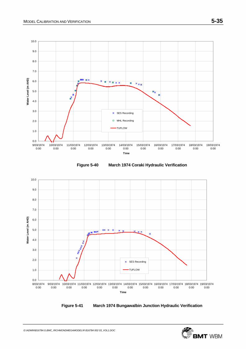
MODEL CALIBRATION AND VERIFICATION 5-35
G:\ADMIN\B16784.G.BMC_RICHMONDMEGAMODEL\R B16784 002 03_VOL1.DOC
Figure 5-40 March 1974 Coraki Hydraulic Verification
Figure 5-41 March 1974 Bungawalbin Junction Hydraulic Verification
0.0
1.0
2.0
3.0
4.0
5.0
6.0
7.0
8.0
9.0
10.0
9/03/19740:00
10/03/19740:00
11/03/19740:00
12/03/19740:00
13/03/19740:00
14/03/19740:00
15/03/19740:00
16/03/19740:00
17/03/19740:00
18/03/19740:00
19/03/19740:00
Time
Wat
er L
evel
(m A
HD
)
SES Recording
MHL Recording
TUFLOW
0.0
1.0
2.0
3.0
4.0
5.0
6.0
7.0
8.0
9.0
10.0
8/03/19740:00
9/03/19740:00
10/03/19740:00
11/03/19740:00
12/03/19740:00
13/03/19740:00
14/03/19740:00
15/03/19740:00
16/03/19740:00
17/03/19740:00
18/03/19740:00
19/03/19740:00
Time
Wat
er L
evel
(m A
HD
)
SES Recording
TUFLOW

MODEL CALIBRATION AND VERIFICATION 5-36
G:\ADMIN\B16784.G.BMC_RICHMONDMEGAMODEL\R B16784 002 03_VOL1.DOC
Figure 5-42 March 1974 Woodburn Hydraulic Verification
Figure 5-43 March 1974 Broadwater Hydraulic Verification
0.0
1.0
2.0
3.0
4.0
5.0
6.0
7.0
8.0
9.0
10.0
9/03/19740:00
10/03/19740:00
11/03/19740:00
12/03/19740:00
13/03/19740:00
14/03/19740:00
15/03/19740:00
16/03/19740:00
17/03/19740:00
18/03/19740:00
19/03/19740:00
Time
Wat
er L
evel
(m A
HD
)
SES Recording
MHL Recording
TUFLOW
0.0
1.0
2.0
3.0
4.0
5.0
6.0
7.0
8.0
9.0
10.0
9/03/19740:00
10/03/19740:00
11/03/19740:00
12/03/19740:00
13/03/19740:00
14/03/19740:00
15/03/19740:00
16/03/19740:00
17/03/19740:00
18/03/19740:00
19/03/19740:00
Time
Wat
er L
evel
(m A
HD
)
SES Recording
TUFLOW
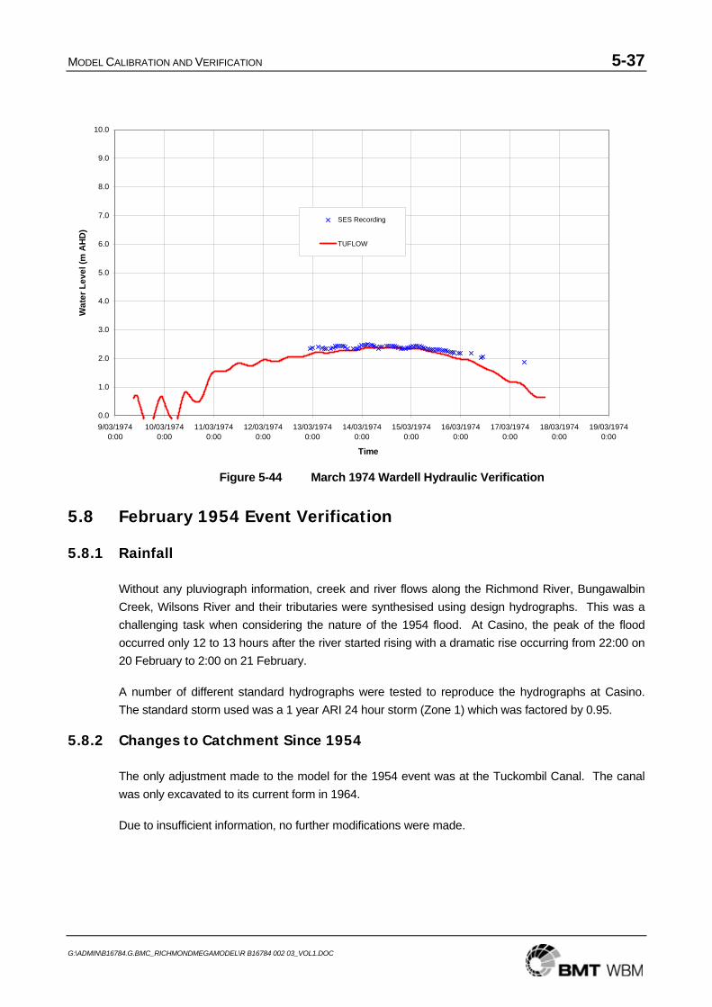
MODEL CALIBRATION AND VERIFICATION 5-37
G:\ADMIN\B16784.G.BMC_RICHMONDMEGAMODEL\R B16784 002 03_VOL1.DOC
Figure 5-44 March 1974 Wardell Hydraulic Verification
5.8 February 1954 Event Verification
5.8.1 Rainfall
Without any pluviograph information, creek and river flows along the Richmond River, Bungawalbin Creek, Wilsons River and their tributaries were synthesised using design hydrographs. This was a challenging task when considering the nature of the 1954 flood. At Casino, the peak of the flood occurred only 12 to 13 hours after the river started rising with a dramatic rise occurring from 22:00 on 20 February to 2:00 on 21 February.
A number of different standard hydrographs were tested to reproduce the hydrographs at Casino. The standard storm used was a 1 year ARI 24 hour storm (Zone 1) which was factored by 0.95.
5.8.2 Changes to Catchment Since 1954
The only adjustment made to the model for the 1954 event was at the Tuckombil Canal. The canal was only excavated to its current form in 1964.
Due to insufficient information, no further modifications were made.
0.0
1.0
2.0
3.0
4.0
5.0
6.0
7.0
8.0
9.0
10.0
9/03/19740:00
10/03/19740:00
11/03/19740:00
12/03/19740:00
13/03/19740:00
14/03/19740:00
15/03/19740:00
16/03/19740:00
17/03/19740:00
18/03/19740:00
19/03/19740:00
Time
Wat
er L
evel
(m A
HD
)
SES Recording
TUFLOW
MODEL CALIBRATION AND VERIFICATION 5-38
G:\ADMIN\B16784.G.BMC_RICHMONDMEGAMODEL\R B16784 002 03_VOL1.DOC
5.8.3 Hydraulic Model Verification
Hydraulic model verification for this event was undertaken using 61 surveyed flood marks as shown on Map 5-31. Peak flood levels are shown on Map 5-32 to Map 5-35 with a summary provided on Map 5-36.
Some features to be noted regarding the hydraulic verification are:
The expansive inundation highlights the magnitude of this event in comparison with the 2009, 2008 and 1974 events;
Upstream from Tatham, there is no recorded data for comparison;
Between Tatham and Coraki, peak flood levels have been reproduced reasonably well considering the assumptions inherent in the modelling;
Within the Wilsons River, there is little recorded data for comparison, although one flood mark is reasonably well reproduced;
Between Coraki and Woodburn, the peak flood levels have been reproduced reasonably well, although some variability is apparent; and
Between Woodburn and Broadwater, and within the Tuckean Swamp, modelled peak flood levels are generally lower that the recorded levels.
5.9 Calibration and Verification Summary
It was found that a lower roughness coefficient applied to the Richmond River upstream from Coraki resulted in a better fit with recorded flood levels during the tidal calibration. However, the lower roughness resulted in a poor fit during flood event simulation. For improved calibration, the higher roughness coefficients were used in that area. This is consistent with the values used for the Mid-Richmond Flood Study.
The four events analysed represent a range of event magnitudes as can be seen from Table 5-3. The combination of these events for calibration and verification use provides confidence that the model has been tested during a range of different flooding conditions.
Manning’s ‘n’ roughness coefficients determined during calibration are presented in Table 5-4. For consistency, the same roughness coefficients were used for all events.
In general, a reasonable calibration has been achieved. Although there is shown to have been significant variability between recorded and modelled flood behaviour in some areas, most differences can be attributed to the limited rainfall data available for some events, and some parts of the catchment.
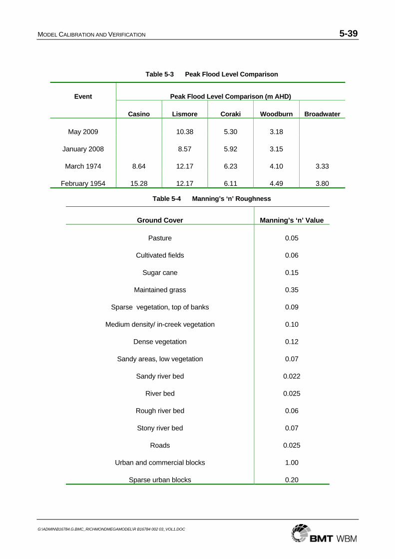
MODEL CALIBRATION AND VERIFICATION 5-39
G:\ADMIN\B16784.G.BMC_RICHMONDMEGAMODEL\R B16784 002 03_VOL1.DOC
Table 5-3 Peak Flood Level Comparison
Peak Flood Level Comparison (m AHD) Event
Casino Lismore Coraki Woodburn Broadwater
May 2009 10.38 5.30 3.18
January 2008 8.57 5.92 3.15
March 1974 8.64 12.17 6.23 4.10 3.33
February 1954 15.28 12.17 6.11 4.49 3.80
Table 5-4 Manning’s ‘n’ Roughness
Ground Cover Manning’s ‘n’ Value
Pasture 0.05
Cultivated fields 0.06
Sugar cane 0.15
Maintained grass 0.35
Sparse vegetation, top of banks 0.09
Medium density/ in-creek vegetation 0.10
Dense vegetation 0.12
Sandy areas, low vegetation 0.07
Sandy river bed
River bed
0.022
0.025
Rough river bed 0.06
Stony river bed 0.07
Roads 0.025
Urban and commercial blocks 1.00
Sparse urban blocks 0.20
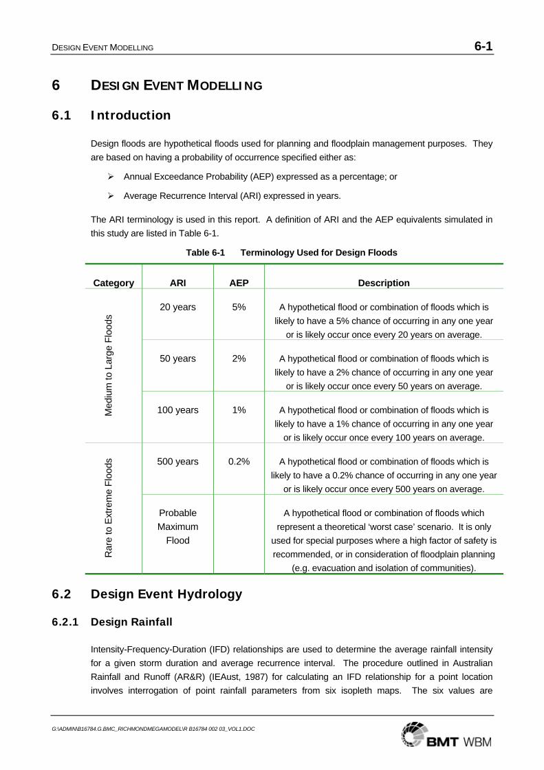
DESIGN EVENT MODELLING 6-1
G:\ADMIN\B16784.G.BMC_RICHMONDMEGAMODEL\R B16784 002 03_VOL1.DOC
6 DESIGN EVENT MODELLING
6.1 Introduction
Design floods are hypothetical floods used for planning and floodplain management purposes. They are based on having a probability of occurrence specified either as:
Annual Exceedance Probability (AEP) expressed as a percentage; or
Average Recurrence Interval (ARI) expressed in years.
The ARI terminology is used in this report. A definition of ARI and the AEP equivalents simulated in this study are listed in Table 6-1.
Table 6-1 Terminology Used for Design Floods
Category ARI AEP Description
20 years 5% A hypothetical flood or combination of floods which is likely to have a 5% chance of occurring in any one year
or is likely occur once every 20 years on average.
50 years 2% A hypothetical flood or combination of floods which is likely to have a 2% chance of occurring in any one year
or is likely occur once every 50 years on average.
Med
ium
to L
arge
Flo
ods
100 years 1% A hypothetical flood or combination of floods which is likely to have a 1% chance of occurring in any one year
or is likely occur once every 100 years on average.
500 years 0.2% A hypothetical flood or combination of floods which is likely to have a 0.2% chance of occurring in any one year
or is likely occur once every 500 years on average.
Rar
e to
Ext
rem
e Fl
oods
Probable Maximum
Flood
A hypothetical flood or combination of floods which represent a theoretical ‘worst case’ scenario. It is only
used for special purposes where a high factor of safety is recommended, or in consideration of floodplain planning
(e.g. evacuation and isolation of communities).
6.2 Design Event Hydrology
6.2.1 Design Rainfall
Intensity-Frequency-Duration (IFD) relationships are used to determine the average rainfall intensity for a given storm duration and average recurrence interval. The procedure outlined in Australian Rainfall and Runoff (AR&R) (IEAust, 1987) for calculating an IFD relationship for a point location involves interrogation of point rainfall parameters from six isopleth maps. The six values are
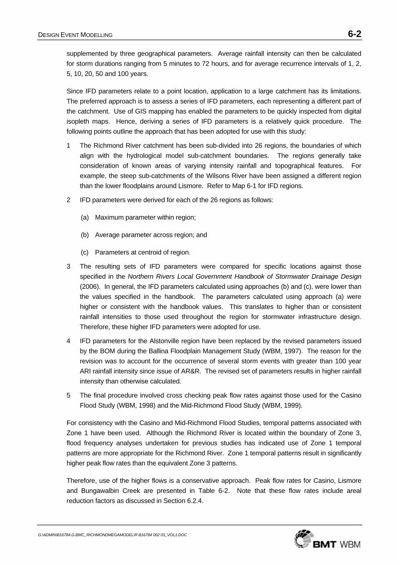
DESIGN EVENT MODELLING 6-2
G:\ADMIN\B16784.G.BMC_RICHMONDMEGAMODEL\R B16784 002 03_VOL1.DOC
supplemented by three geographical parameters. Average rainfall intensity can then be calculated for storm durations ranging from 5 minutes to 72 hours, and for average recurrence intervals of 1, 2, 5, 10, 20, 50 and 100 years.
Since IFD parameters relate to a point location, application to a large catchment has its limitations. The preferred approach is to assess a series of IFD parameters, each representing a different part of the catchment. Use of GIS mapping has enabled the parameters to be quickly inspected from digital isopleth maps. Hence, deriving a series of IFD parameters is a relatively quick procedure. The following points outline the approach that has been adopted for use with this study:
1 The Richmond River catchment has been sub-divided into 26 regions, the boundaries of which align with the hydrological model sub-catchment boundaries. The regions generally take consideration of known areas of varying intensity rainfall and topographical features. For example, the steep sub-catchments of the Wilsons River have been assigned a different region than the lower floodplains around Lismore. Refer to Map 6-1 for IFD regions.
2 IFD parameters were derived for each of the 26 regions as follows:
(a) Maximum parameter within region;
(b) Average parameter across region; and
(c) Parameters at centroid of region.
3 The resulting sets of IFD parameters were compared for specific locations against those specified in the Northern Rivers Local Government Handbook of Stormwater Drainage Design (2006). In general, the IFD parameters calculated using approaches (b) and (c), were lower than the values specified in the handbook. The parameters calculated using approach (a) were higher or consistent with the handbook values. This translates to higher than or consistent rainfall intensities to those used throughout the region for stormwater infrastructure design. Therefore, these higher IFD parameters were adopted for use.
4 IFD parameters for the Alstonville region have been replaced by the revised parameters issued by the BOM during the Ballina Floodplain Management Study (WBM, 1997). The reason for the revision was to account for the occurrence of several storm events with greater than 100 year ARI rainfall intensity since issue of AR&R. The revised set of parameters results in higher rainfall intensity than otherwise calculated.
5 The final procedure involved cross checking peak flow rates against those used for the Casino Flood Study (WBM, 1998) and the Mid-Richmond Flood Study (WBM, 1999).
For consistency with the Casino and Mid-Richmond Flood Studies, temporal patterns associated with Zone 1 have been used. Although the Richmond River is located within the boundary of Zone 3, flood frequency analyses undertaken for previous studies has indicated use of Zone 1 temporal patterns are more appropriate for the Richmond River. Zone 1 temporal patterns result in significantly higher peak flow rates than the equivalent Zone 3 patterns.
Therefore, use of the higher flows is a conservative approach. Peak flow rates for Casino, Lismore and Bungawalbin Creek are presented in Table 6-2. Note that these flow rates include areal reduction factors as discussed in Section 6.2.4.
DESIGN EVENT MODELLING 6-3
G:\ADMIN\B16784.G.BMC_RICHMONDMEGAMODEL\R B16784 002 03_VOL1.DOC
Table 6-2 100 Year ARI Design Event Peak Flow Rates
Peak Flow Rates (m3/s) and Critical Event Duration Location
Mid-Richmond Flood Study
Casino Flood Study
Current Study
Casino 3,950 (48 hr) 4,430 (36hr) 4,370 (48hr)
Lismore 6,475 (48hr) - 4,800 (48hr)
Bungawalbin 2,520 (48hr) - 1,485 (72hr)
The comparison between estimated flow rates is discussed below.
Casino – peak flow rates estimated for this study are higher than used for the Mid-Richmond Flood Study and comparable to the Casino Flood Study.
Lismore – peak flow rates estimated for this study are approximately 75% of the Mid-Richmond Flood Study peak flows. This is due to the significant attenuation of runoff throughout the Wilsons River catchment, as described in Section 5. This attenuation was not represented in the Lismore Flood Study (Sinclair Knight and Partners, 1993) hydrologic modelling used for the Mid-Richmond Flood Study. The current peak flow rates are consistent with the results of the calibration event flows. Refer to Section 6.8 for further discussion.
Bungawalbin – peak flow rates estimated for this study are approximately 60% of the Mid-Richmond Flood Study peak flows. Again this is due to the significant attenuation of runoff in the Bungawalbin as discussed in Section 5. The current peak flow rates are consistent with the results of the calibration event flows. Refer to Section 6.8 for further discussion.
6.2.2 PMF Estimation
The probable maximum precipitation (PMP) is defined as ‘the greatest depth of precipitation for a given duration meteorologically possible for a given storm area at a particular location at a particular time of year’ (WMO, 1986). The PMP is used to estimate the probable maximum flood (PMF), representing an extreme flood that can be expected to occur on average once every 10,000 to 1,000,000 years, depending on the catchment.
The two methods recommended for calculation of the PMP along the East Coast of Australia are:
Generalised Short Duration Method (GSDM); and
Generalised Tropical Storm Method Revised (GTSMR).
As the name implies, the GSDM is used for short duration events on catchments up to 1,000km2. More applicable to the 7,000km2 Richmond River catchment is the GTSMR, which is recommended for event durations up to 120 hours.
Presented in Table 6-3, are the total PMP rainfall depths for the Richmond River. Also shown in Table 6-3 are the rainfall depths for the 20, 50, 100 and 500 year ARI events for comparison. The
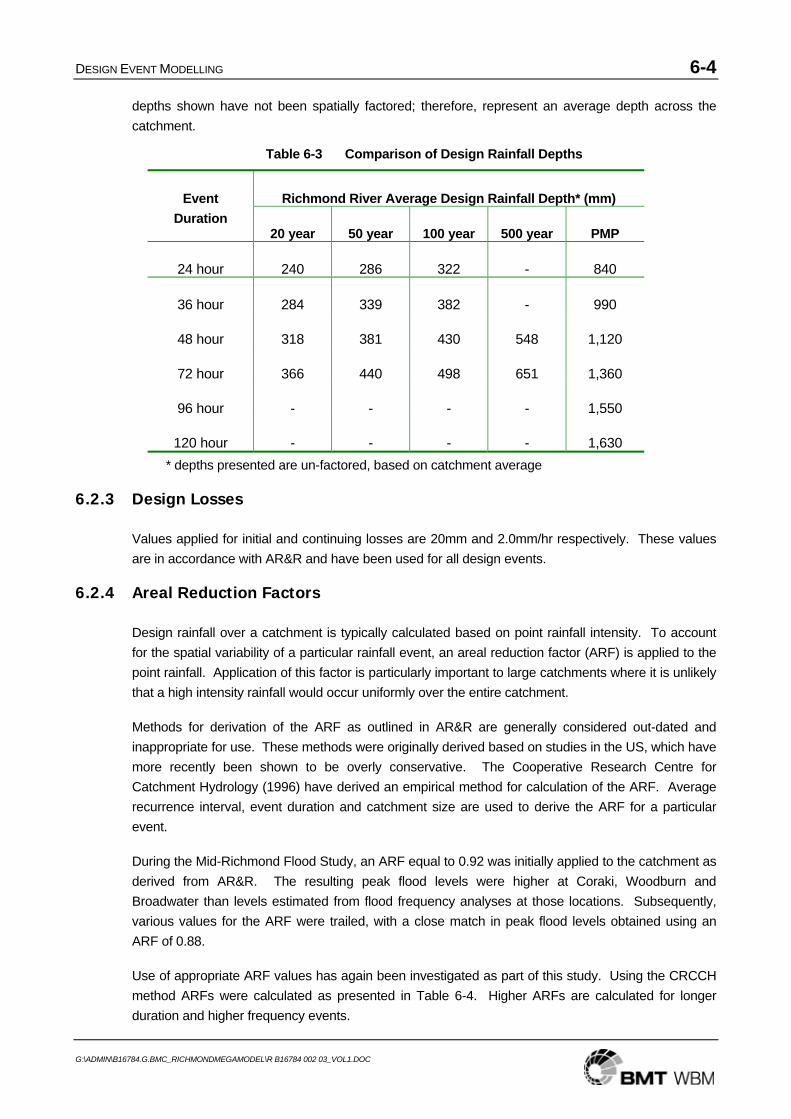
DESIGN EVENT MODELLING 6-4
G:\ADMIN\B16784.G.BMC_RICHMONDMEGAMODEL\R B16784 002 03_VOL1.DOC
depths shown have not been spatially factored; therefore, represent an average depth across the catchment.
Table 6-3 Comparison of Design Rainfall Depths
Richmond River Average Design Rainfall Depth* (mm) Event Duration
20 year 50 year 100 year 500 year PMP
24 hour 240 286 322 - 840
36 hour 284 339 382 - 990
48 hour 318 381 430 548 1,120
72 hour 366 440 498 651 1,360
96 hour - - - - 1,550
120 hour - - - - 1,630 * depths presented are un-factored, based on catchment average
6.2.3 Design Losses
Values applied for initial and continuing losses are 20mm and 2.0mm/hr respectively. These values are in accordance with AR&R and have been used for all design events.
6.2.4 Areal Reduction Factors
Design rainfall over a catchment is typically calculated based on point rainfall intensity. To account for the spatial variability of a particular rainfall event, an areal reduction factor (ARF) is applied to the point rainfall. Application of this factor is particularly important to large catchments where it is unlikely that a high intensity rainfall would occur uniformly over the entire catchment.
Methods for derivation of the ARF as outlined in AR&R are generally considered out-dated and inappropriate for use. These methods were originally derived based on studies in the US, which have more recently been shown to be overly conservative. The Cooperative Research Centre for Catchment Hydrology (1996) have derived an empirical method for calculation of the ARF. Average recurrence interval, event duration and catchment size are used to derive the ARF for a particular event.
During the Mid-Richmond Flood Study, an ARF equal to 0.92 was initially applied to the catchment as derived from AR&R. The resulting peak flood levels were higher at Coraki, Woodburn and Broadwater than levels estimated from flood frequency analyses at those locations. Subsequently, various values for the ARF were trailed, with a close match in peak flood levels obtained using an ARF of 0.88.
Use of appropriate ARF values has again been investigated as part of this study. Using the CRCCH method ARFs were calculated as presented in Table 6-4. Higher ARFs are calculated for longer duration and higher frequency events.
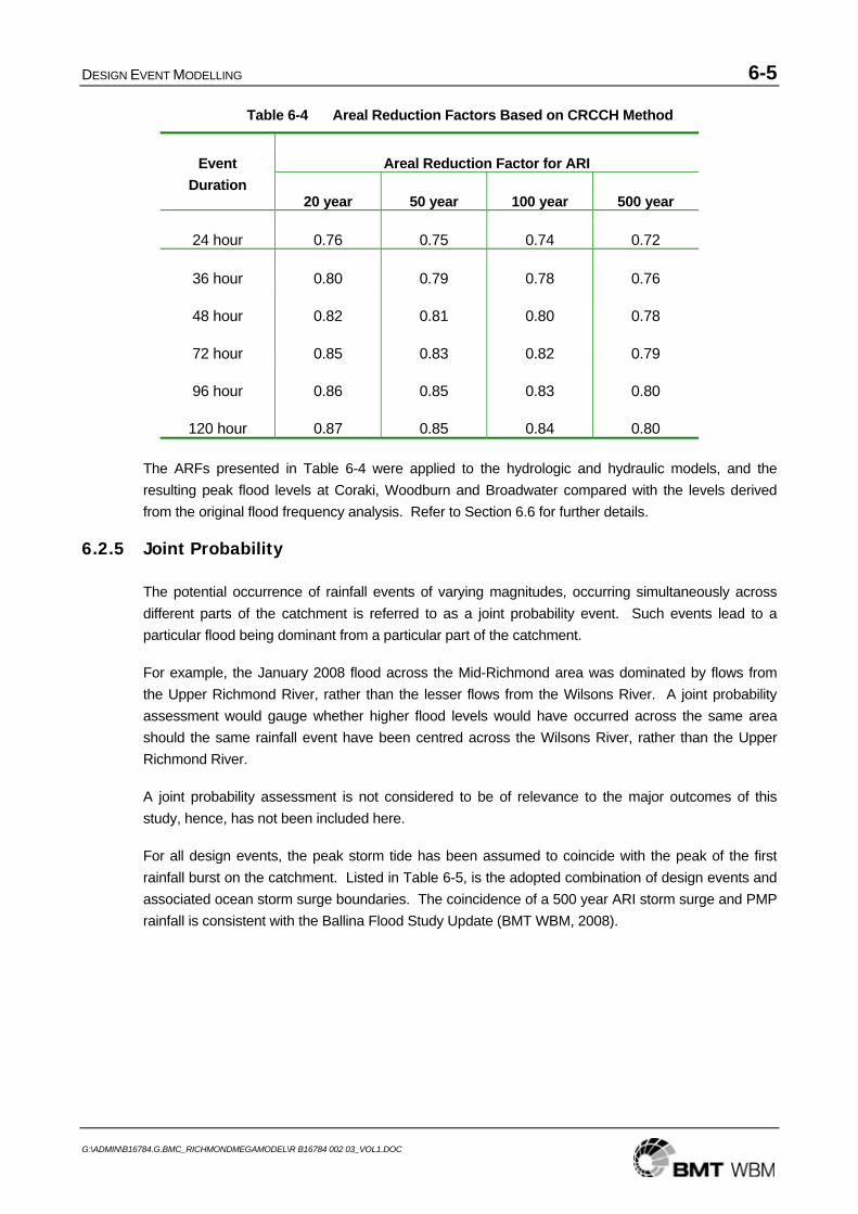
DESIGN EVENT MODELLING 6-5
G:\ADMIN\B16784.G.BMC_RICHMONDMEGAMODEL\R B16784 002 03_VOL1.DOC
Table 6-4 Areal Reduction Factors Based on CRCCH Method
Areal Reduction Factor for ARI Event Duration
20 year 50 year 100 year 500 year
24 hour 0.76 0.75 0.74 0.72
36 hour 0.80 0.79 0.78 0.76
48 hour 0.82 0.81 0.80 0.78
72 hour 0.85 0.83 0.82 0.79
96 hour 0.86 0.85 0.83 0.80
120 hour 0.87 0.85 0.84 0.80
The ARFs presented in Table 6-4 were applied to the hydrologic and hydraulic models, and the resulting peak flood levels at Coraki, Woodburn and Broadwater compared with the levels derived from the original flood frequency analysis. Refer to Section 6.6 for further details.
6.2.5 Joint Probability
The potential occurrence of rainfall events of varying magnitudes, occurring simultaneously across different parts of the catchment is referred to as a joint probability event. Such events lead to a particular flood being dominant from a particular part of the catchment.
For example, the January 2008 flood across the Mid-Richmond area was dominated by flows from the Upper Richmond River, rather than the lesser flows from the Wilsons River. A joint probability assessment would gauge whether higher flood levels would have occurred across the same area should the same rainfall event have been centred across the Wilsons River, rather than the Upper Richmond River.
A joint probability assessment is not considered to be of relevance to the major outcomes of this study, hence, has not been included here.
For all design events, the peak storm tide has been assumed to coincide with the peak of the first rainfall burst on the catchment. Listed in Table 6-5, is the adopted combination of design events and associated ocean storm surge boundaries. The coincidence of a 500 year ARI storm surge and PMP rainfall is consistent with the Ballina Flood Study Update (BMT WBM, 2008).
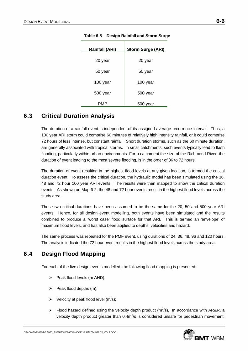
DESIGN EVENT MODELLING 6-6
G:\ADMIN\B16784.G.BMC_RICHMONDMEGAMODEL\R B16784 002 03_VOL1.DOC
Table 6-5 Design Rainfall and Storm Surge
Rainfall (ARI) Storm Surge (ARI)
20 year 20 year
50 year 50 year
100 year 100 year
500 year 500 year
PMP 500 year
6.3 Critical Duration Analysis
The duration of a rainfall event is independent of its assigned average recurrence interval. Thus, a 100 year ARI storm could comprise 60 minutes of relatively high intensity rainfall, or it could comprise 72 hours of less intense, but constant rainfall. Short duration storms, such as the 60 minute duration, are generally associated with tropical storms. In small catchments, such events typically lead to flash flooding, particularly within urban environments. For a catchment the size of the Richmond River, the duration of event leading to the most severe flooding, is in the order of 36 to 72 hours.
The duration of event resulting in the highest flood levels at any given location, is termed the critical duration event. To assess the critical duration, the hydraulic model has been simulated using the 36, 48 and 72 hour 100 year ARI events. The results were then mapped to show the critical duration events. As shown on Map 6-2, the 48 and 72 hour events result in the highest flood levels across the study area.
These two critical durations have been assumed to be the same for the 20, 50 and 500 year ARI events. Hence, for all design event modelling, both events have been simulated and the results combined to produce a ‘worst case’ flood surface for that ARI. This is termed an ‘envelope’ of maximum flood levels, and has also been applied to depths, velocities and hazard.
The same process was repeated for the PMF event, using durations of 24, 36, 48, 96 and 120 hours. The analysis indicated the 72 hour event results in the highest flood levels across the study area.
6.4 Design Flood Mapping
For each of the five design events modelled, the following flood mapping is presented:
Peak flood levels (m AHD);
Peak flood depths (m);
Velocity at peak flood level (m/s);
Flood hazard defined using the velocity depth product (m2/s). In accordance with AR&R, a velocity depth product greater than 0.4m2/s is considered unsafe for pedestrian movement.
DESIGN EVENT MODELLING 6-7
G:\ADMIN\B16784.G.BMC_RICHMONDMEGAMODEL\R B16784 002 03_VOL1.DOC
Thus, areas with velocity depth products exceeding this value are presented as ‘high hazard’; and
Flood hazard defined using criteria outlined in the NSW Floodplain Development Manual. High and low hazard areas are defined using flow velocity and depth, although with different parameters than the velocity depth product method.
Peak flood levels and velocity depth product hazard mapping from the Lismore Flood Study (Patterson Britton, 2002) are also presented for the Lismore area.
The interpretation of maps within this report should be done with an appreciation of any limitations with their accuracy. Whilst the points below highlight these limitations, it is important to note that the results presented provide a current prediction of design flood behaviour:
Recognition that no two floods behave in exactly the same manner;
Design floods are a ‘best estimate’ of an average flood for their probability of occurrence; and
Approximations and assumptions are made in the modelling and mapping process as discussed throughout this report.
6.4.1 20 Year ARI
All mapping for the 20 year ARI combined 48 and 72 hour events is included digitally on the addendum CD. The following mapping is included:
Peak flood levels are presented on Maps 6-33 to 6-36;
Peak flood depths are presented on Maps 6-37 to 6-40;
Velocities at peak flood level are presented on Maps 6-41 to 6-44;
Velocity depth product hazard categories are presented on Maps 6-45 to 6-48; and
Floodplain Development Manual hazard categories are presented on Maps 6-49 to 6-52.
6.4.2 50 Year ARI
All mapping for the 50 year ARI combined 48 and 72 hour events is included digitally on the addendum CD. The following mapping is included:
Peak flood levels are presented on Maps 6-53 to 6-56;
Peak flood depths are presented on Maps 6-57 to 6-60;
Velocities at peak flood level are presented on Maps 6-61 to 6-64;
Velocity depth product hazard categories are presented on Maps 6-65 to 6-68; and
Floodplain Development Manual hazard categories are presented on Maps 6-69 to 6-72.
DESIGN EVENT MODELLING 6-8
G:\ADMIN\B16784.G.BMC_RICHMONDMEGAMODEL\R B16784 002 03_VOL1.DOC
6.4.3 100 Year ARI
All mapping for the 100 year ARI combined 48 and 72 hour events is included in Volume 2 of this report and digitally on the addendum CD. The following mapping is included:
Peak flood levels are presented on Maps 6-3 to 6-6;
Peak flood depths are presented on Maps 6-7 to 6-10;
Velocities at peak flood level are presented on Maps 6-11 to 6-14;
Velocity depth product hazard categories are presented on Maps 6-15 to 6-18; and
Floodplain Development Manual hazard categories are presented on Maps 6-19 to 6-22.
6.4.4 500 Year ARI
All mapping for the 500 year ARI combined 48 and 72 hour events is included digitally on the addendum CD. The following mapping is included:
Peak flood levels are presented on Maps 6-73 to 6-76;
Peak flood depths are presented on Maps 6-77 to 6-80;
Velocities at peak flood level are presented on Maps 6-81 to 6-84;
Velocity depth product hazard categories are presented on Maps 6-85 to 6-88; and
Floodplain Development Manual hazard categories are presented on Maps 6-89 to 6-92.
6.4.5 Probable Maximum Flood
All mapping for the 72 hour PMF event is included digitally on the addendum CD. The following mapping is included:
Peak flood levels are presented on Maps 6-93 to 6-96;
Peak flood depths are presented on Maps 6-97 to 6-100;
Velocities at peak flood level are presented on Maps 6-101 to 6-104;
Velocity depth product hazard categories are presented on Maps 6-105 to 6-108; and
Floodplain Development Manual hazard categories are presented on Maps 6-109 to 6-112.
During the PMF event, the coastal dunes downstream from Broadwater are breached allowing floodwaters on the lower floodplain to flow directly into the ocean. No allowance has been made for scouring of the dunes, thus, the peak flood levels presented in the mapping are conservative estimates.
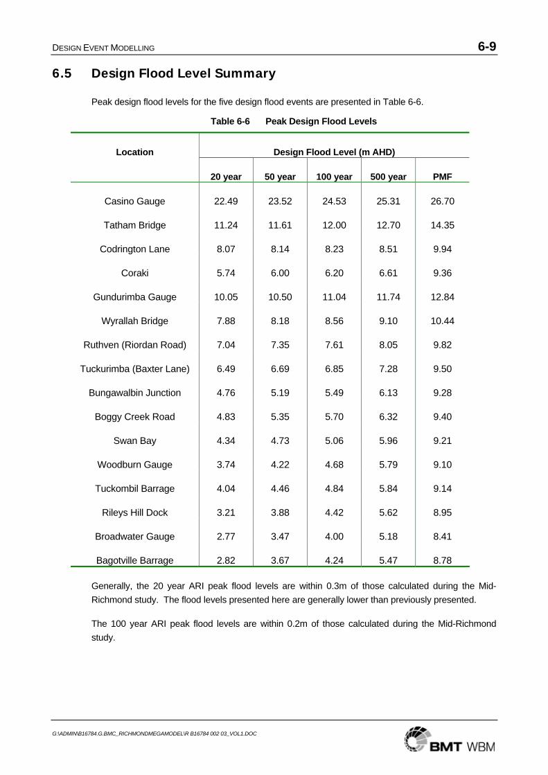
DESIGN EVENT MODELLING 6-9
G:\ADMIN\B16784.G.BMC_RICHMONDMEGAMODEL\R B16784 002 03_VOL1.DOC
6.5 Design Flood Level Summary
Peak design flood levels for the five design flood events are presented in Table 6-6.
Table 6-6 Peak Design Flood Levels
Design Flood Level (m AHD) Location
20 year 50 year 100 year 500 year PMF
Casino Gauge 22.49 23.52 24.53 25.31 26.70
Tatham Bridge 11.24 11.61 12.00 12.70 14.35
Codrington Lane 8.07 8.14 8.23 8.51 9.94
Coraki 5.74 6.00 6.20 6.61 9.36
Gundurimba Gauge 10.05 10.50 11.04 11.74 12.84
Wyrallah Bridge 7.88 8.18 8.56 9.10 10.44
Ruthven (Riordan Road) 7.04 7.35 7.61 8.05 9.82
Tuckurimba (Baxter Lane) 6.49 6.69 6.85 7.28 9.50
Bungawalbin Junction 4.76 5.19 5.49 6.13 9.28
Boggy Creek Road 4.83 5.35 5.70 6.32 9.40
Swan Bay 4.34 4.73 5.06 5.96 9.21
Woodburn Gauge 3.74 4.22 4.68 5.79 9.10
Tuckombil Barrage 4.04 4.46 4.84 5.84 9.14
Rileys Hill Dock 3.21 3.88 4.42 5.62 8.95
Broadwater Gauge 2.77 3.47 4.00 5.18 8.41
Bagotville Barrage 2.82 3.67 4.24 5.47 8.78
Generally, the 20 year ARI peak flood levels are within 0.3m of those calculated during the Mid-Richmond study. The flood levels presented here are generally lower than previously presented.
The 100 year ARI peak flood levels are within 0.2m of those calculated during the Mid-Richmond study.
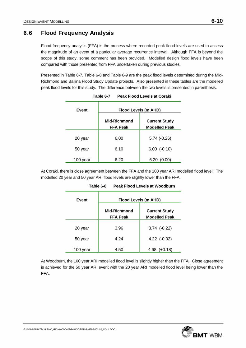
DESIGN EVENT MODELLING 6-10
G:\ADMIN\B16784.G.BMC_RICHMONDMEGAMODEL\R B16784 002 03_VOL1.DOC
6.6 Flood Frequency Analysis
Flood frequency analysis (FFA) is the process where recorded peak flood levels are used to assess the magnitude of an event of a particular average recurrence interval. Although FFA is beyond the scope of this study, some comment has been provided. Modelled design flood levels have been compared with those presented from FFA undertaken during previous studies.
Presented in Table 6-7, Table 6-8 and Table 6-9 are the peak flood levels determined during the Mid-Richmond and Ballina Flood Study Update projects. Also presented in these tables are the modelled peak flood levels for this study. The difference between the two levels is presented in parenthesis.
Table 6-7 Peak Flood Levels at Coraki
Flood Levels (m AHD) Event
Mid-Richmond FFA Peak
Current Study Modelled Peak
20 year 6.00 5.74 (-0.26)
50 year 6.10 6.00 (-0.10)
100 year 6.20 6.20 (0.00)
At Coraki, there is close agreement between the FFA and the 100 year ARI modelled flood level. The modelled 20 year and 50 year ARI flood levels are slightly lower than the FFA.
Table 6-8 Peak Flood Levels at Woodburn
Flood Levels (m AHD) Event
Mid-Richmond FFA Peak
Current Study Modelled Peak
20 year 3.96 3.74 (-0.22)
50 year 4.24 4.22 (-0.02)
100 year 4.50 4.68 (+0.18)
At Woodburn, the 100 year ARI modelled flood level is slightly higher than the FFA. Close agreement is achieved for the 50 year ARI event with the 20 year ARI modelled flood level being lower than the FFA.
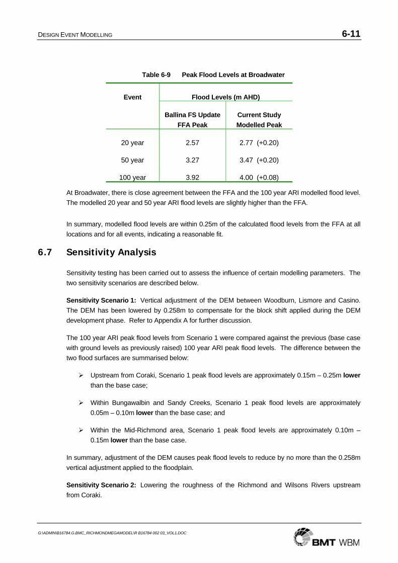
DESIGN EVENT MODELLING 6-11
G:\ADMIN\B16784.G.BMC_RICHMONDMEGAMODEL\R B16784 002 03_VOL1.DOC
Table 6-9 Peak Flood Levels at Broadwater
Flood Levels (m AHD) Event
Ballina FS Update FFA Peak
Current Study Modelled Peak
20 year 2.57 2.77 (+0.20)
50 year 3.27 3.47 (+0.20)
100 year 3.92 4.00 (+0.08)
At Broadwater, there is close agreement between the FFA and the 100 year ARI modelled flood level. The modelled 20 year and 50 year ARI flood levels are slightly higher than the FFA.
In summary, modelled flood levels are within 0.25m of the calculated flood levels from the FFA at all locations and for all events, indicating a reasonable fit.
6.7 Sensitivity Analysis
Sensitivity testing has been carried out to assess the influence of certain modelling parameters. The two sensitivity scenarios are described below.
Sensitivity Scenario 1: Vertical adjustment of the DEM between Woodburn, Lismore and Casino. The DEM has been lowered by 0.258m to compensate for the block shift applied during the DEM development phase. Refer to Appendix A for further discussion.
The 100 year ARI peak flood levels from Scenario 1 were compared against the previous (base case with ground levels as previously raised) 100 year ARI peak flood levels. The difference between the two flood surfaces are summarised below:
Upstream from Coraki, Scenario 1 peak flood levels are approximately 0.15m – 0.25m lower than the base case;
Within Bungawalbin and Sandy Creeks, Scenario 1 peak flood levels are approximately 0.05m – 0.10m lower than the base case; and
Within the Mid-Richmond area, Scenario 1 peak flood levels are approximately 0.10m – 0.15m lower than the base case.
In summary, adjustment of the DEM causes peak flood levels to reduce by no more than the 0.258m vertical adjustment applied to the floodplain.
Sensitivity Scenario 2: Lowering the roughness of the Richmond and Wilsons Rivers upstream from Coraki.
DESIGN EVENT MODELLING 6-12
G:\ADMIN\B16784.G.BMC_RICHMONDMEGAMODEL\R B16784 002 03_VOL1.DOC
Similarly, the 100 year ARI peak flood levels from Scenario 2 were compared against the previous 100 year ARI peak flood levels. The difference between the two flood surfaces are summarised below:
Upstream from Coraki, Scenario 2 peak flood levels are up to 0.70m lower than the base case;
Within Bungawalbin and Sandy Creeks, Scenario 2 peak flood levels are approximately 0.05m – 0.20m lower than the base case; and
Within the Mid-Richmond area, Scenario 2 peak flood levels are approximately 0.05m – 0.10m higher than the base case.
In summary, use of the base case flood levels is a conservative approach across all areas except the Mid-Richmond. Across the Mid-Richmond area, Scenario 2 results are within 0.1m of the base case results, thus, indicating no significant difference.
6.8 Climate Change Assessment
At the time of writing, the most current guidelines relating to the impact of climate change is the Practical Considerations of Climate Change released by DECC in 2007 (DECC, 2007). In the guidelines, it is recommended that a climate change assessment consider the impacts of an increase in sea level and an increase in rainfall intensity.
Sea Level Rise
Current predictions of future sea level rise vary considerably based on which emission scenario is being considered. In February 2009, DECCW published a Draft Sea Level Rise Policy Statement (DECC, 2009), to be adopted for planning decisions accounting for climate change. The guideline specifies sea level rise values to be adopted for planning decisions to 2050 and 2100.
The adopted values are realistic as CSIRO tracking in recent years has shown that sea level rise trends follow the ‘A2’ line. The guideline values accounts for the estimated global mean (IPCC, 2007), predicted regional variation (CSIRO, 2009) and accelerated ice sheet contribution (IPCC, 2007) to the increase in sea level.
The DECCW draft guideline values for sea level rise are:
2050 (+ 0.40m); and
2100 (+ 0.90m).
Rainfall Intensity Increase
Similar to the sea level rise guidelines, DECCW has released estimates for changes in rainfall intensity for extreme rainfall event. These estimates were assessed by the CSIRO and documented in the NSW Climate Change in Australia series (CSIRO, 2007a and 2007b). A summary of the main findings documented in the climate change series of reports are also listed in Practical Considerations of Climate Change (DECC, 2007).
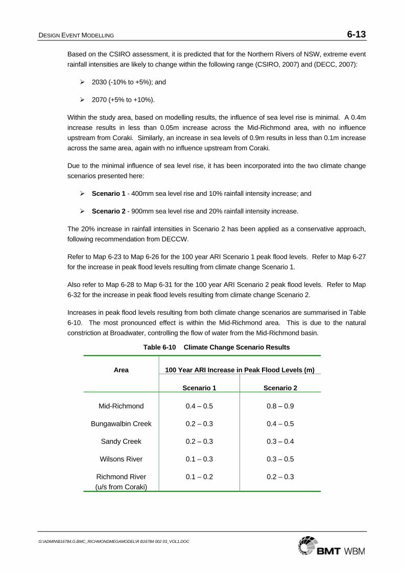
DESIGN EVENT MODELLING 6-13
G:\ADMIN\B16784.G.BMC_RICHMONDMEGAMODEL\R B16784 002 03_VOL1.DOC
Based on the CSIRO assessment, it is predicted that for the Northern Rivers of NSW, extreme event rainfall intensities are likely to change within the following range (CSIRO, 2007) and (DECC, 2007):
2030 (-10% to +5%); and
2070 (+5% to +10%).
Within the study area, based on modelling results, the influence of sea level rise is minimal. A 0.4m increase results in less than 0.05m increase across the Mid-Richmond area, with no influence upstream from Coraki. Similarly, an increase in sea levels of 0.9m results in less than 0.1m increase across the same area, again with no influence upstream from Coraki.
Due to the minimal influence of sea level rise, it has been incorporated into the two climate change scenarios presented here:
Scenario 1 - 400mm sea level rise and 10% rainfall intensity increase; and
Scenario 2 - 900mm sea level rise and 20% rainfall intensity increase.
The 20% increase in rainfall intensities in Scenario 2 has been applied as a conservative approach, following recommendation from DECCW.
Refer to Map 6-23 to Map 6-26 for the 100 year ARI Scenario 1 peak flood levels. Refer to Map 6-27 for the increase in peak flood levels resulting from climate change Scenario 1.
Also refer to Map 6-28 to Map 6-31 for the 100 year ARI Scenario 2 peak flood levels. Refer to Map 6-32 for the increase in peak flood levels resulting from climate change Scenario 2.
Increases in peak flood levels resulting from both climate change scenarios are summarised in Table 6-10. The most pronounced effect is within the Mid-Richmond area. This is due to the natural constriction at Broadwater, controlling the flow of water from the Mid-Richmond basin.
Table 6-10 Climate Change Scenario Results
100 Year ARI Increase in Peak Flood Levels (m) Area
Scenario 1 Scenario 2
Mid-Richmond 0.4 – 0.5 0.8 – 0.9
Bungawalbin Creek 0.2 – 0.3 0.4 – 0.5
Sandy Creek 0.2 – 0.3 0.3 – 0.4
Wilsons River 0.1 – 0.3 0.3 – 0.5
Richmond River (u/s from Coraki)
0.1 – 0.2 0.2 – 0.3
CONCLUSION 7-1
G:\ADMIN\B16784.G.BMC_RICHMONDMEGAMODEL\R B16784 002 03_VOL1.DOC
7 CONCLUSION
A hydrologic and an integrated one and two-dimensional (1D/2D) hydraulic flood model have been developed for the Richmond River catchment between Broadwater, Casino and Lismore. The models have been jointly calibrated to a 1994 tidal cycle and the May 2009 flood event. The models were further verified against the 1954, 1974 and 2008 flood events. In general, a reasonable calibration has been achieved.
Design flood behaviour is presented for the 20, 50, 100 and 500 year average recurrence interval (ARI) events and the probable maximum flood. Sensitivity testing and a climate change assessment have also been carried out for the 100 year ARI event.
Key issues and findings from the study are:
Data Collection
A digital elevation model (DEM) has been produced for the floodplain extending from Ballina to Casino and Lismore. The DEM is based on a combination of existing datasets including airborne laser scanning (ALS), photogrammetry and ground survey, as well as recent photogrammetry obtained for the specific purposes of this study.
Testing of the recent photogrammetric survey was undertaken using ground survey captured for the Mid-Richmond Flood Study. Application of a 258mm vertical block shift was used to achieve conformance with the specified accuracy of +/- 0.26m.
Hydrologic Modelling
The movement of flood waters through the Wilsons River catchment is shown to be approximately three times slower than in the Richmond River upstream of Casino. This is primarily due to floodplain storage, rather than slope or stream length.
Calibration of the Wilsons River hydrologic model has shown lower flow rates than previously published. Cross checking of the calculated flow rates for historical events, against recorded flows using the Bureau of Meteorology’s rating curve shows good agreement.
There is significant storage within the Bungawalbin Creek catchment, although the ability to model flood behaviour is limited by the shortage of rainfall and streamflow data.
A preliminary review of radar rainfall records highlights the variability of rainfall across the Bungawalbin catchment. Hence, representation of the rainfall using a sparse coverage of pluviographs has introduced uncertainty with the model calibration. Therefore, conservative hydrologic model parameters have been adopted to allow for the inherent uncertainties.
CONCLUSION 7-2
G:\ADMIN\B16784.G.BMC_RICHMONDMEGAMODEL\R B16784 002 03_VOL1.DOC
Hydraulic Modelling
A reasonable model calibration has been achieved using similar model parameters as adopted in the Mid-Richmond Flood Study (WBM Oceanics, 1999) and the Ballina Flood Study Update (BMT WBM, 2008).
Design flood behaviour shows good agreement with modelling previously presented in the Mid-Richmond Flood Study.
During the PMF event, the coastal dunes downstream from Broadwater are shown to be breached.
Sensitivity testing of a decrease in bed roughness in both the Wilsons and Richmond Rivers upstream from Coraki shows decreased peak flood levels of up to 0.7m upstream from Coraki, and increased peak flood levels of up to 0.1m in the Mid-Richmond basin.
Sensitivity testing of the applied DEM block shift generally indicates less than 0.2m difference in peak flood levels.
Current projections for sea level rise of 0.4m by 2050 and 0.9m by 2100 have been assessed. Upstream from Broadwater, these projections result in less than 0.05m and 0.1m increase to peak flood levels respectively during the 100 year ARI event.
Potential increases to rainfall intensity of 10 and 20 percent have also been assessed. The resulting peak flood levels upstream of Broadwater are shown to increase by up to 0.5m and 0.9m respectively.
In summary, the hydrologic and hydraulic models have been developed with due consideration to their ongoing use for floodplain management. Whilst the sensitivity testing has shown the potential for higher peak flood levels than presented in the design event mapping, the increases are within the current 0.5m freeboard requirement applicable to habitable floor levels (NSW Floodplain Development Manual, 2005). The potential for increases in rainfall intensity have been shown to significantly affect peak flood levels beyond the current freeboard requirement.
It is, therefore, recommended that the outcomes of this study, including an appropriate allowance for climate change, are considered in the preparation and review of all floodplain development policies.
ACKNOWLEDGEMENTS 8-1
G:\ADMIN\B16784.G.BMC_RICHMONDMEGAMODEL\R B16784 002 03_VOL1.DOC
8 ACKNOWLEDGEMENTS
The project team would like to thank the following organisations for their assistance with this project:
Ballina Shire Council;
Bureau of Meteorology;
Lismore City Council
Manly Hydraulics Laboratory;
NSW Department of Environment, Climate Change and Water;
NSW Roads and Traffic Authority;
Richmond River County Council;
Richmond Valley Council;
Rous Water; and
State Emergency Service.
In addition, the land holders and residents of the Richmond Valley who contributed information to this study are gratefully acknowledged. The information provided has been fundamental to the outcomes of this study.
REFERENCES 9-1
G:\ADMIN\B16784.G.BMC_RICHMONDMEGAMODEL\R B16784 002 03_VOL1.DOC
9 REFERENCES Report of the Richmond River Valley Flood Mitigation Committee (Department of Public
Works, 1954 & 1958)
NSW Coastal Rivers Flood Plain Management Studies, Richmond Valley (Sinclair Knight and Partners, 1980)
Richmond Valley Flood Problems (Richmond River Inter-Departmental Committee, 1982)
Lismore Flood Study and Floodplain Management (Sinclair Knight Merz ,1993)
Ballina Floodplain Management Study (WBM Oceanics, 1997)
Casino Flood Study (WBM Oceanics, 1998)
Lismore Levee Scheme Environmental Impact Statement (WBM Oceanics, 1999)
Mid-Richmond Flood Study (WBM Oceanics, 1999)
Casino Floodplain Risk Management Study (WBM Oceanics, 2001)
Lismore Floodplain Management Study (Patterson Britton, 2001)
Mid-Richmond Floodplain Management Study (WBM Oceanics, 2002)
Wardell and Cabbage Tree Island Floodplain Management Study (Patterson Britton, 2004)
Tuckombil Canal Flood Affect Assessment (WBM Oceanics 2005)
Richmond River Data Compilation Study (WBM, 2006)
Ballina Flood Study Update (BMT WBM, 2008)

DISCUSSION PAPER ON SURVEY DATA A-1
G:\ADMIN\B16784.G.BMC_RICHMONDMEGAMODEL\R B16784 002 03_VOL1.DOC
APPENDIX A: DISCUSSION PAPER ON SURVEY DATA
INTRODUCTION A-1-1
A.1 INTRODUCTION
In January 2008, BMT WBM were commissioned by Richmond River County Council (RRCC) to undertake the Richmond River Flood Model and Rural Flood Mapping Study. For simplicity, the name of the study has been shortened to the Richmond River Flood Mapping Study.
For the study, a dynamically linked one and two-dimensional (1D/2D) flood model is being developed for the following areas:
• Richmond River between Casino and Broadwater (not including Casino);
• Bungawalbin Creek from Yellow Crossing to the Richmond River;
• Wilsons River from Lismore to Coraki (not including Lismore); and
• Lower reaches of other major tributaries of the Richmond River, such as Deep Creek and Sandy Creek.
The study area is shown on Map A1-1. In addition to these areas, the model will be extended along the Richmond River and Evans River to the ocean using a 1D model network. In total, the model will include approximately 160km of river and 210km of major creeks.
The initial stages of the flood modelling process involved collating various topographic and hydrographic survey data sources for the production of a digital elevation model (DEM). A critical part of this process is an assessment of the accuracy of the data.
This discussion paper has been prepared to document the sources of data as well as the quality assurance processes applied for checking the accuracy of the data. Finally, the methods used for combining the data sources are discussed, including the priority assigned to each where survey regions overlap.
SURVEY DATA ACQUISITION A-2-1
A.2 SURVEY DATA ACQUISITION
A.2.1 Hydrographic Survey
Hydrographic survey of the Richmond River and associate tributaries was collected in 2004 for the NSW Department of Natural Resources’ Estuary Program. The hydrographic, or bathymetric, survey consists of depth soundings taken from a boat. Therefore, the extent of the survey was limited to all waterways accessible by boat, which is approximately the same as the tidal extents of the Richmond River system. Extents of the survey include:
• Richmond River from Casino to the river mouth at Ballina (107km);
• Wilsons River from the Richmond River to 49.7km upstream;
• Bungawalbin Creek from the Richmond River to 34.3km upstream;
• Sandy Creek from Bungawalbin Creek to 5.6km upstream;
• Leycester Creek from the Wilsons River to 13.8km upstream;
• Rocky Mouth Creek from the Richmond River to 4.0km upstream;
• Tuckean Broadwater from the Richmond River to 4.5km upstream;
• North Creek from the Richmond River to 19.1km upstream;
• Emigrant Creek from the Richmond River to Tintenbar (22.7km);
• Maguires Creek from Emigrant Creek to 6.0km upstream;
• Duck Creek from Emigrant Creek to 2.7km upstream; and
• The North Creek Canal at Ballina (3.5km).
In the lower 9km of the Richmond River, survey was acquired at 10m centres along parallel tracking lines at 20m spacing. A coarser resolution of cross sections at 100m centres was used for:
• Richmond River upstream to Rocky Mouth Creek (33.7km);
• Tuckean Broadwater;
• North Creek – lower 6.7km; and
• The North Creek Canal.
Elsewhere, cross sections were captured at approximately 250m centres. Extents of the hydrographic survey are shown on Map A2-1.
Beyond the extents of the hydrographic survey, additional cross sections of creeks have been extracted from the MIKE11 hydraulic model developed for the Mid-Richmond Flood Study. These cross sections were digitised for that study from hardcopy drawings produced by the Public Works Department in 1980.
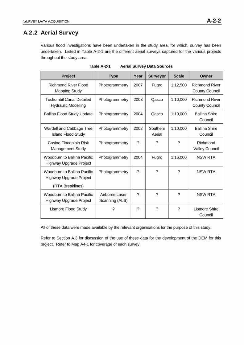
SURVEY DATA ACQUISITION A-2-2
A.2.2 Aerial Survey
Various flood investigations have been undertaken in the study area, for which, survey has been undertaken. Listed in Table A-2-1 are the different aerial surveys captured for the various projects throughout the study area.
Table A-2-1 Aerial Survey Data Sources
Project Type Year Surveyor Scale Owner
Richmond River Flood Mapping Study
Photogrammetry 2007 Fugro 1:12,500 Richmond River County Council
Tuckombil Canal Detailed Hydraulic Modelling
Photogrammetry 2003 Qasco 1:10,000 Richmond River County Council
Ballina Flood Study Update Photogrammetry 2004 Qasco 1:10,000 Ballina Shire Council
Wardell and Cabbage Tree Island Flood Study
Photogrammetry 2002 Southern Aerial
1:10,000 Ballina Shire Council
Casino Floodplain Risk Management Study
Photogrammetry ? ? ? Richmond Valley Council
Woodburn to Ballina Pacific Highway Upgrade Project
Photogrammetry 2004 Fugro 1:16,000 NSW RTA
Woodburn to Ballina Pacific Highway Upgrade Project
(RTA Breaklines)
Photogrammetry ? ? ? NSW RTA
Woodburn to Ballina Pacific Highway Upgrade Project
Airborne Laser Scanning (ALS)
? ? ? NSW RTA
Lismore Flood Study ? ? ? ? Lismore Shire Council
All of these data were made available by the relevant organisations for the purpose of this study.
Refer to Section A.3 for discussion of the use of these data for the development of the DEM for this project. Refer to Map A4-1 for coverage of each survey.
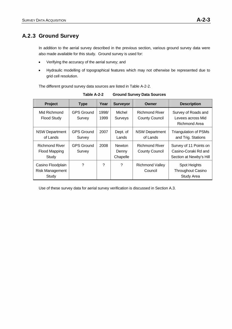
SURVEY DATA ACQUISITION A-2-3
A.2.3 Ground Survey
In addition to the aerial survey described in the previous section, various ground survey data were also made available for this study. Ground survey is used for:
• Verifying the accuracy of the aerial survey; and
• Hydraulic modelling of topographical features which may not otherwise be represented due to grid cell resolution.
The different ground survey data sources are listed in Table A-2-2.
Table A-2-2 Ground Survey Data Sources
Project Type Year Surveyor Owner Description
Mid Richmond Flood Study
GPS Ground Survey
1998/1999
Michel Surveys
Richmond River County Council
Survey of Roads and Levees across Mid
Richmond Area
NSW Department of Lands
GPS Ground Survey
2007 Dept. of Lands
NSW Department of Lands
Triangulation of PSMs and Trig. Stations
Richmond River Flood Mapping
Study
GPS Ground Survey
2008 Newton Denny
Chapelle
Richmond River County Council
Survey of 11 Points on Casino-Coraki Rd and Section at Newby’s Hill
Casino Floodplain Risk Management
Study
? ? ? Richmond Valley Council
Spot Heights Throughout Casino
Study Area
Use of these survey data for aerial survey verification is discussed in Section A.3.
SURVEY DATA ANALYSIS A-3-1
A.3 SURVEY DATA ANALYSIS
A.3.1 Hydrographic Survey
Due to the lack of independent hydrographic survey, no analysis has been undertaken on the hydrographic survey.
A.3.2 Topographic Survey
The focus of the aerial survey data verification process has been on the photogrammetry captured for this project. It is assumed that accuracy and verification checks have previously been performed on the aerial survey captured for other projects.
The originally photogrammetry for this study was provided to BMT WBM in November 2007. Verification was first undertaken using the 974 points of the 1998 ground survey.
Firstly, the points were manually filtered to exclude all points located on the following terrain:
• Long grass, scrub or coarse vegetation;
• Steep or irregular / undulating terrain; and
• Bridges or other structures.
All remaining points are located on flat surfaces, such as roads and levees. The elevations of these 651 points were, therefore, suitable to compare against the corresponding elevation from the photogrammetry.
A triangulated irregular network (TIN) was produced from the photogrammetry, and a point inspection carried out. The point inspection process extracts the elevation from the photogrammetry at each point location. The ground survey elevation is subtracted from the corresponding TIN elevation, which results in a residual. The residual is the relative difference between the two data sources.
Of all 651 points, the average difference was found to be -0.262m with a root-mean-square (RMS) equal to 0.330m. Given the specification for the survey was for an accuracy to +/-0.260m (one standard deviation), it was apparent that further checks would be required. Refer to Map A3-1 for thematic map of the residuals between the 1998 ground survey and the original photogrammetry.
The mean difference indicated that the photogrammetry was, on average, 0.262m lower than the equivalent ground survey elevation. It was expected that this systematic error would to be close to zero.
To determine the source of the systematic error, a series of checks were undertaken, comparing the datum assigned to each of the following three ground survey datasets:
• 1998 ground survey;
• Department of Lands survey of permanent survey marks (PSMs), and
• Control survey used for the photogrammetry.
SURVEY DATA ANALYSIS A-3-2
All survey was confirmed to be relative to the Australian Height Datum (AHD). Further, the control used for both the 1998 survey and photogrammetry control survey datasets were found to agree closely with the Department of Lands survey of the PSMs.
In March 2008, RRCC commissioned an independent surveyor to provide survey at two locations:
• Eleven points along the Casino-Coraki Road. This location was chosen as the mean difference between the photogrammetry and 1998 ground survey was -0.514m. Although the triangulation process and the cross fall of the road could be expected to cause a slight difference between the two datasets, a mean difference of this magnitude clearly indicated error in one of the datasets.
• A line of 16 points extending from the Richmond River onto the floodplain at Newby’s Hill near the confluence with Bungawalbin Creek. This location was chosen to represent a range of different land uses.
Refer to Map A2-2 for survey locations. Labels on the screen plots are as follows:
• Pink text with white halo – photogrammetry breakline levels;
• Black text with pink halo – elevation from triangulated photogrammetry; and
• Red text with yellow halo – 2008 independent survey levels.
A comparison between the independent survey elevations and the photogrammetry showed a mean difference equal to -0.536m. Hence, the 2008 independent survey showed close agreement with the 1998 ground survey.
Additionally, the mean difference of the 16 points across the floodplain was -0.335m.
Following extensive discussion with the photogrammetrist and commission of Emeritus Professor John Fryer as an independent expert, it was agreed that the photogrammetrist would apply additional control to the aerial triangulation solution of the photogrammetry. BMT WBM selected 38 ground control points across the survey region to supplement the 16 points used for the original solution. A further 30 points were supplied to the photogrammetrist for checking of the revised photogrammetry.
Refer to Appendix B for minutes of the aerial survey.
In July 2008, the revised photogrammetry was supplied to BMT WBM. The same procedure was applied for checking using the 651 points of the 1998 ground survey. The mean difference and RMS of the 38 control points, 30 checking points and complete 651 point dataset is presented in Table A-3-1.
When checked against the complete 651 point dataset, the reissued photogrammetry showed little improvement from the original photogrammetry. The mean difference was -0.258m.
Following discussion with the project team and with the advice of the independent expert, it was decided to apply a block shift to the photogrammetry, elevating the entire dataset by the mean difference of -0.258m. Thus, the mean difference would be reduced to zero, and the RMS equal to 0.256m was marginally within the +/-0.260m specification.
Refer to Map A3-2 for a thematic map of the residuals between the 1998 ground survey and the elevated photogrammetry.
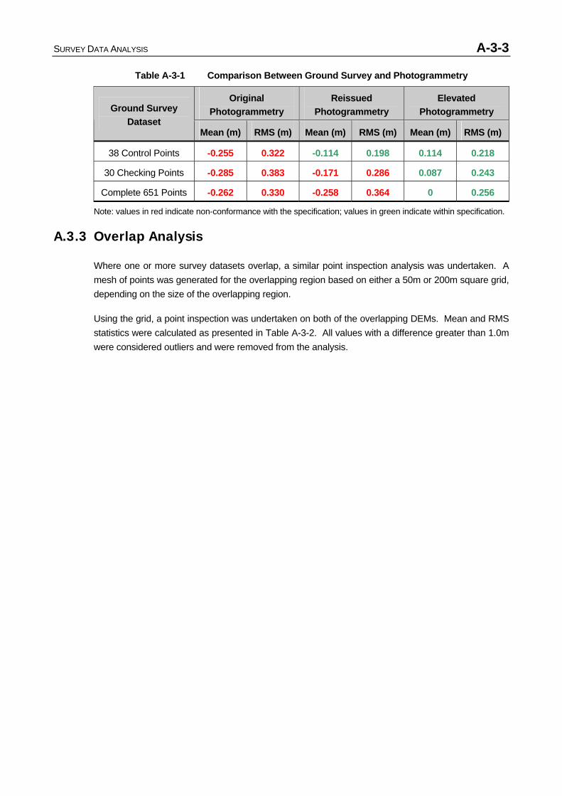
SURVEY DATA ANALYSIS A-3-3
Table A-3-1 Comparison Between Ground Survey and Photogrammetry
Original Photogrammetry
Reissued Photogrammetry
Elevated Photogrammetry Ground Survey
Dataset Mean (m) RMS (m) Mean (m) RMS (m) Mean (m) RMS (m)
38 Control Points -0.255 0.322 -0.114 0.198 0.114 0.218
30 Checking Points -0.285 0.383 -0.171 0.286 0.087 0.243
Complete 651 Points -0.262 0.330 -0.258 0.364 0 0.256
Note: values in red indicate non-conformance with the specification; values in green indicate within specification.
A.3.3 Overlap Analysis
Where one or more survey datasets overlap, a similar point inspection analysis was undertaken. A mesh of points was generated for the overlapping region based on either a 50m or 200m square grid, depending on the size of the overlapping region.
Using the grid, a point inspection was undertaken on both of the overlapping DEMs. Mean and RMS statistics were calculated as presented in Table A-3-2. All values with a difference greater than 1.0m were considered outliers and were removed from the analysis.
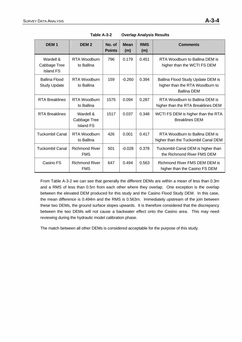
SURVEY DATA ANALYSIS A-3-4
Table A-3-2 Overlap Analysis Results
DEM 1 DEM 2 No. of Points
Mean (m)
RMS (m)
Comments
Wardell & Cabbage Tree
Island FS
RTA Woodburn to Ballina
796 0.179 0.451 RTA Woodburn to Ballina DEM is higher than the WCTI FS DEM
Ballina Flood Study Update
RTA Woodburn to Ballina
159 -0.260 0.394 Ballina Flood Study Update DEM is higher than the RTA Woodburn to
Ballina DEM
RTA Breaklines RTA Woodburn to Ballina
1575 0.094 0.287 RTA Woodburn to Ballina DEM is higher than the RTA Breaklines DEM
RTA Breaklines Wardell & Cabbage Tree
Island FS
1517 0.037 0.348 WCTI FS DEM is higher than the RTA Breaklines DEM
Tuckombil Canal RTA Woodburn to Ballina
426 0.001 0.417 RTA Woodburn to Ballina DEM is higher than the Tuckombil Canal DEM
Tuckombil Canal Richmond River FMS
501 -0.028 0.378 Tuckombil Canal DEM is higher than the Richmond River FMS DEM
Casino FS Richmond River FMS
647 0.494 0.563 Richmond River FMS DEM DEM is higher than the Casino FS DEM
From Table A-3-2 we can see that generally the different DEMs are within a mean of less than 0.3m and a RMS of less than 0.5m from each other where they overlap. One exception is the overlap between the elevated DEM produced for this study and the Casino Flood Study DEM. In this case, the mean difference is 0.494m and the RMS is 0.563m. Immediately upstream of the join between these two DEMs, the ground surface slopes upwards. It is therefore considered that the discrepancy between the two DEMs will not cause a backwater effect onto the Casino area. This may need reviewing during the hydraulic model calibration phase.
The match between all other DEMs is considered acceptable for the purpose of this study.
DIGITAL ELEVATION MODEL DEVELOPMENT A-4-1
A.4 DIGITAL ELEVATION MODEL DEVELOPMENT
A.4.1 General Approach
Although multiple DEMs covering different parts of the study area can be used for the hydraulic modelling process, it is generally good practice to combine the data sources into one DEM. This reduces the potential for error, and is also beneficial for mapping purposes. Therefore, following the accuracy verification process, a broader DEM was produced from the many smaller DEMs within the study area.
Capture of aerial survey does not allow determination of bathymetry. The hydrographic survey can then be used to represent river and creek bathymetry between the banks. Since the hydraulic modelling for this project will represent all rivers and creeks as 1D model components, incorporation of the hydrographic survey into the broader DEM was not necessary. This process was undertaken for the Ballina Flood Study Update since the lower Richmond River was modelled in 2D. The Ballina DEM can be seen on Map A4-6.
A.4.2 Survey Data Priority
It is acknowledged that the different survey data were captured for different projects, each having different accuracy specifications. Therefore, an important part of the DEM composition process is assigning priority levels to survey data which overlap with other survey datasets.
Generally, there is little overlap between the different surveys, with the exception of the Woodburn area. Therefore, in the overlap areas it was necessary to determine which survey is considered more accurate and should be given the highest priority level.
Consideration of the aerial survey scale is the biggest factor in determining the accuracy of each survey. An exception to this is the more recently captured survey for this project. The priority levels assigned to each data source is shown in Table A-4-1. The DEM composition is shown on Map A4-1.
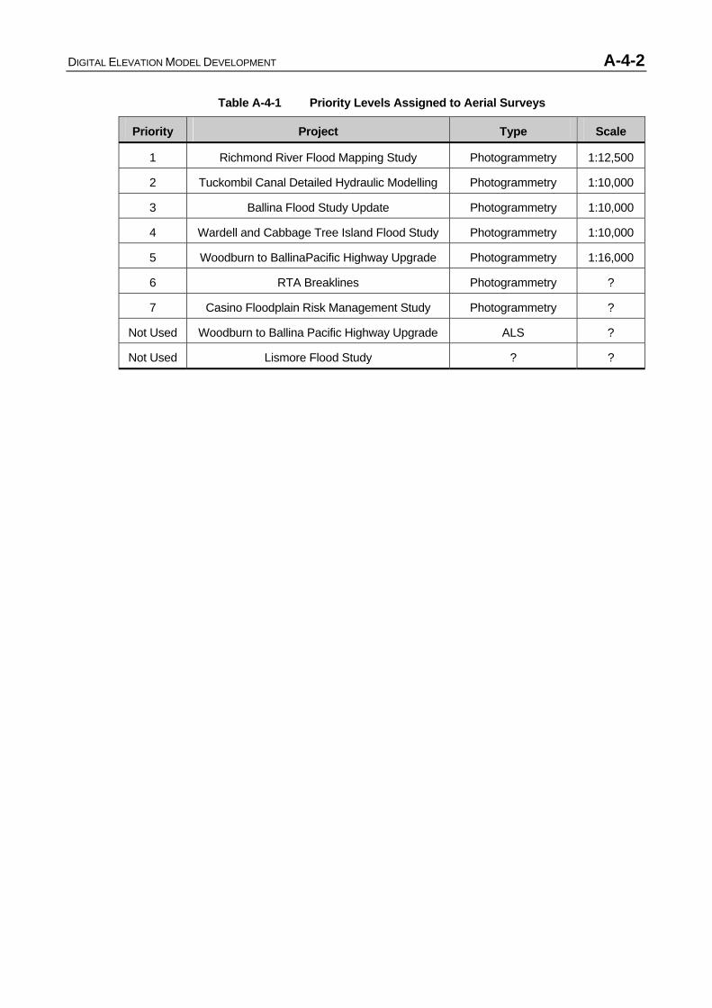
DIGITAL ELEVATION MODEL DEVELOPMENT A-4-2
Table A-4-1 Priority Levels Assigned to Aerial Surveys
Priority Project Type Scale
1 Richmond River Flood Mapping Study Photogrammetry 1:12,500
2 Tuckombil Canal Detailed Hydraulic Modelling Photogrammetry 1:10,000
3 Ballina Flood Study Update Photogrammetry 1:10,000
4 Wardell and Cabbage Tree Island Flood Study Photogrammetry 1:10,000
5 Woodburn to BallinaPacific Highway Upgrade Photogrammetry 1:16,000
6 RTA Breaklines Photogrammetry ?
7 Casino Floodplain Risk Management Study Photogrammetry ?
Not Used Woodburn to Ballina Pacific Highway Upgrade ALS ?
Not Used Lismore Flood Study ? ?
DIGITAL ELEVATION MODEL DEVELOPMENT A-4-3
The final DEM is shown on the following figures:
• Map A4-2 – Richmond River between Casino and Tatham, including Deep Creek;
• Map A4-3 – Richmond River from Tatham to Coraki, including the Wilsons River and Tuckean Swamp;
• Map A4-4 – Richmond River from Coraki to Woodburn, including Bungawalbin and Sandy Creeks;
• Map A4-5- Richmond River from Coraki to Broadwater, including the Evans River and Rocky Mouth Creek; and
• Map A4-6 – Lower Richmond River from Wardell to Ballina.
A.4.3 Merging DEMs
Where DEMs were merged, the following principles were applied:
• Where possible, join lines were located along roads, levees or watercourses;
• Where no distinct topographic feature was present and a discrepancy between the two surfaces existed, the two surfaces were merged over a distance of up to 100m. The distance used, depended upon the elevation difference between the two DEMs and other local topography; and
• Merging was generally applied over the lower priority DEM.
An essential part of the merging process was ensuring key topographic features, or hydraulic controls, were not removed.
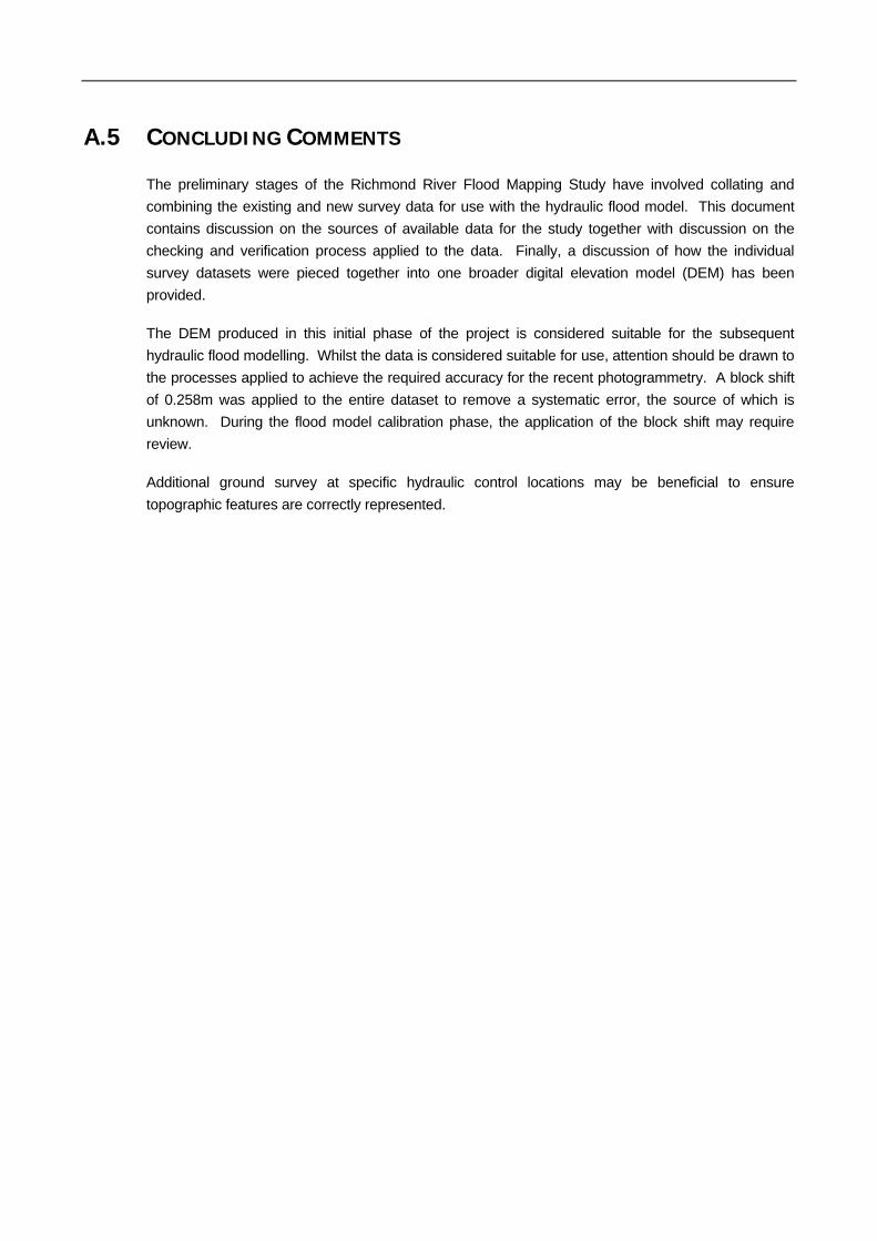
A.5 CONCLUDING COMMENTS
The preliminary stages of the Richmond River Flood Mapping Study have involved collating and combining the existing and new survey data for use with the hydraulic flood model. This document contains discussion on the sources of available data for the study together with discussion on the checking and verification process applied to the data. Finally, a discussion of how the individual survey datasets were pieced together into one broader digital elevation model (DEM) has been provided.
The DEM produced in this initial phase of the project is considered suitable for the subsequent hydraulic flood modelling. Whilst the data is considered suitable for use, attention should be drawn to the processes applied to achieve the required accuracy for the recent photogrammetry. A block shift of 0.258m was applied to the entire dataset to remove a systematic error, the source of which is unknown. During the flood model calibration phase, the application of the block shift may require review.
Additional ground survey at specific hydraulic control locations may be beneficial to ensure topographic features are correctly represented.

TIDAL CALIBRATION RESULTS B-1
G:\ADMIN\B16784.G.BMC_RICHMONDMEGAMODEL\R B16784 002 03_VOL1.DOC
-1
-0.75
-0.5
-0.25
0
0.25
0.5
0.75
1
3/11/199400:00
3/11/199403:00
3/11/199406:00
3/11/199409:00
3/11/199412:00
3/11/199415:00
3/11/199418:00
3/11/199421:00
4/11/199400:00
Time
Wat
er L
evel
(m A
HD
)
Recorded Data
Modelled Levels
-2000
-1500
-1000
-500
0
500
1000
1500
3/11/1994 0:00 3/11/1994 3:00 3/11/1994 6:00 3/11/1994 9:00 3/11/1994 12:00 3/11/1994 15:00 3/11/1994 18:00 3/11/1994 21:00 4/11/1994 0:00
Time
Dis
char
ge (c
umec
s)
Recorded Data
Modelled Discharge
APPENDIX B: TIDAL CALIBRATION RESULTS
Figure B-1 Site 1: Richmond River Entrance - Water Levels
Figure B-2 Site 1: Richmond River Entrance – Discharge
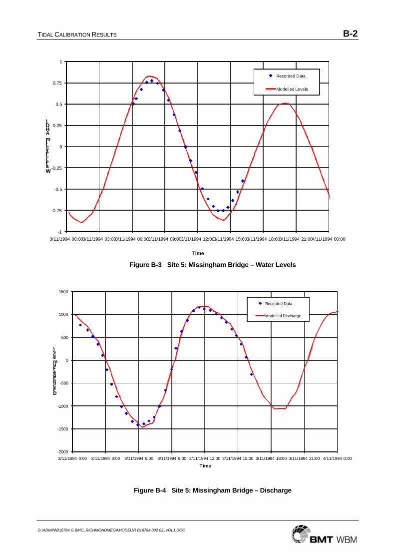
TIDAL CALIBRATION RESULTS B-2
G:\ADMIN\B16784.G.BMC_RICHMONDMEGAMODEL\R B16784 002 03_VOL1.DOC
-1
-0.75
-0.5
-0.25
0
0.25
0.5
0.75
1
3/11/1994 00:003/11/1994 03:003/11/1994 06:003/11/1994 09:003/11/1994 12:003/11/1994 15:003/11/1994 18:003/11/1994 21:004/11/1994 00:00
Water Level (m AHD)
Time
Recorded Data
Modelled Levels
-2000
-1500
-1000
-500
0
500
1000
1500
3/11/1994 0:00 3/11/1994 3:00 3/11/1994 6:00 3/11/1994 9:00 3/11/1994 12:00 3/11/1994 15:00 3/11/1994 18:00 3/11/1994 21:00 4/11/1994 0:00
Discharge (cumecs)
Time
Recorded Data
Modelled Discharge
Figure B-3 Site 5: Missingham Bridge – Water Levels
Figure B-4 Site 5: Missingham Bridge – Discharge
TIDAL CALIBRATION RESULTS B-3
G:\ADMIN\B16784.G.BMC_RICHMONDMEGAMODEL\R B16784 002 03_VOL1.DOC
-1
-0.75
-0.5
-0.25
0
0.25
0.5
0.75
1
3/11/199400:00
3/11/199403:00
3/11/199406:00
3/11/199409:00
3/11/199412:00
3/11/199415:00
3/11/199418:00
3/11/199421:00
4/11/199400:00
Time
Wat
er L
evel
(m A
HD
)
Recorded Data
Modelled Levels
-1
-0.75
-0.5
-0.25
0
0.25
0.5
0.75
1
3/11/199400:00
3/11/199403:00
3/11/199406:00
3/11/199409:00
3/11/199412:00
3/11/199415:00
3/11/199418:00
3/11/199421:00
4/11/199400:00
Time
Wat
er L
evel
(m A
HD
)
Recorded Data
Modelled Levels
Figure B-5 Site 7: Burns Point – Water Levels
Figure B-6 Site 13: Broadwater – Water Levels
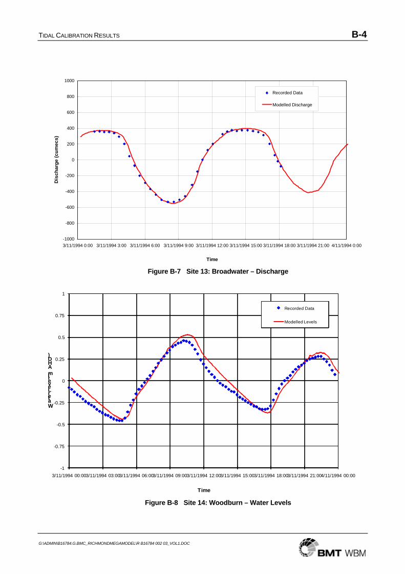
TIDAL CALIBRATION RESULTS B-4
G:\ADMIN\B16784.G.BMC_RICHMONDMEGAMODEL\R B16784 002 03_VOL1.DOC
-1000
-800
-600
-400
-200
0
200
400
600
800
1000
3/11/1994 0:00 3/11/1994 3:00 3/11/1994 6:00 3/11/1994 9:00 3/11/1994 12:00 3/11/1994 15:00 3/11/1994 18:00 3/11/1994 21:00 4/11/1994 0:00
Time
Dis
char
ge (c
umec
s)
Recorded Data
Modelled Discharge
-1
-0.75
-0.5
-0.25
0
0.25
0.5
0.75
1
3/11/1994 00:003/11/1994 03:003/11/1994 06:003/11/1994 09:003/11/1994 12:003/11/1994 15:003/11/1994 18:003/11/1994 21:004/11/1994 00:00
Water Level (m AHD)
Time
Recorded Data
Modelled Levels
Figure B-7 Site 13: Broadwater – Discharge
Figure B-8 Site 14: Woodburn – Water Levels
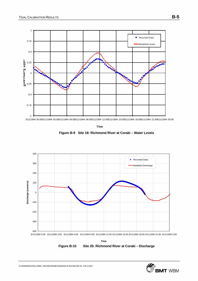
TIDAL CALIBRATION RESULTS B-5
G:\ADMIN\B16784.G.BMC_RICHMONDMEGAMODEL\R B16784 002 03_VOL1.DOC
-1
-0.75
-0.5
-0.25
0
0.25
0.5
0.75
1
3/11/1994 00:003/11/1994 03:003/11/1994 06:003/11/1994 09:003/11/1994 12:003/11/1994 15:003/11/1994 18:003/11/1994 21:004/11/1994 00:00
Water Level (m AHD)
Time
Recorded Data
Modelled Levels
-400
-300
-200
-100
0
100
200
300
400
3/11/1994 0:00 3/11/1994 3:00 3/11/1994 6:00 3/11/1994 9:00 3/11/1994 12:00 3/11/1994 15:00 3/11/1994 18:00 3/11/1994 21:00 4/11/1994 0:00
Time
Dis
char
ge (c
umec
s)
Recorded Data
Modelled Discharge
Figure B-9 Site 18: Richmond River at Coraki – Water Levels
Figure B-10 Site 25: Richmond River at Coraki – Discharge
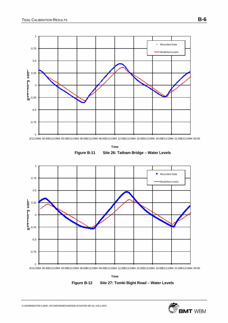
TIDAL CALIBRATION RESULTS B-6
G:\ADMIN\B16784.G.BMC_RICHMONDMEGAMODEL\R B16784 002 03_VOL1.DOC
-1
-0.75
-0.5
-0.25
0
0.25
0.5
0.75
1
3/11/1994 00:003/11/1994 03:003/11/1994 06:003/11/1994 09:003/11/1994 12:003/11/1994 15:003/11/1994 18:003/11/1994 21:004/11/1994 00:00
Water Level (m AHD)
Time
Recorded Data
Modelled Levels
-1
-0.75
-0.5
-0.25
0
0.25
0.5
0.75
1
3/11/1994 00:003/11/1994 03:003/11/1994 06:003/11/1994 09:003/11/1994 12:003/11/1994 15:003/11/1994 18:003/11/1994 21:004/11/1994 00:00
Water Level (m AHD)
Time
Recorded Data
Modelled Levels
Figure B-11 Site 26: Tatham Bridge – Water Levels
Figure B-12 Site 27: Tomki Bight Road – Water Levels
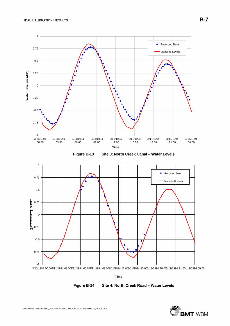
TIDAL CALIBRATION RESULTS B-7
G:\ADMIN\B16784.G.BMC_RICHMONDMEGAMODEL\R B16784 002 03_VOL1.DOC
-1
-0.75
-0.5
-0.25
0
0.25
0.5
0.75
1
3/11/199400:00
3/11/199403:00
3/11/199406:00
3/11/199409:00
3/11/199412:00
3/11/199415:00
3/11/199418:00
3/11/199421:00
4/11/199400:00
Time
Wat
er L
evel
(m A
HD
)
Recorded Data
Modelled Levels
-1
-0.75
-0.5
-0.25
0
0.25
0.5
0.75
1
3/11/1994 00:003/11/1994 03:003/11/1994 06:003/11/1994 09:003/11/1994 12:003/11/1994 15:003/11/1994 18:003/11/1994 21:004/11/1994 00:00
Water Level (m AHD)
Time
Recorded Data
Modelled Levels
Figure B-13 Site 3: North Creek Canal – Water Levels
Figure B-14 Site 4: North Creek Road – Water Levels
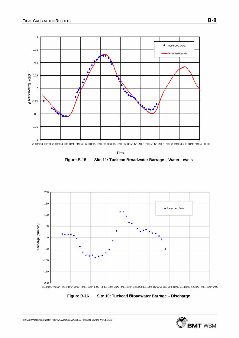
TIDAL CALIBRATION RESULTS B-8
G:\ADMIN\B16784.G.BMC_RICHMONDMEGAMODEL\R B16784 002 03_VOL1.DOC
-1
-0.75
-0.5
-0.25
0
0.25
0.5
0.75
1
3/11/1994 00:003/11/1994 03:003/11/1994 06:003/11/1994 09:003/11/1994 12:003/11/1994 15:003/11/1994 18:003/11/1994 21:004/11/1994 00:00
Water Level (m AHD)
Time
Recorded Data
Modelled Levels
-200
-150
-100
-50
0
50
100
150
200
3/11/1994 0:00 3/11/1994 3:00 3/11/1994 6:00 3/11/1994 9:00 3/11/1994 12:00 3/11/1994 15:00 3/11/1994 18:00 3/11/1994 21:00 4/11/1994 0:00
Time
Dis
char
ge (c
umec
s)
Recorded Data
Figure B-15 Site 11: Tuckean Broadwater Barrage – Water Levels
Figure B-16 Site 10: Tuckean Broadwater Barrage – Discharge
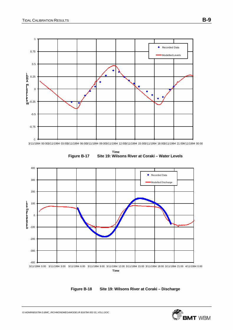
TIDAL CALIBRATION RESULTS B-9
G:\ADMIN\B16784.G.BMC_RICHMONDMEGAMODEL\R B16784 002 03_VOL1.DOC
-1
-0.75
-0.5
-0.25
0
0.25
0.5
0.75
1
3/11/1994 00:003/11/1994 03:003/11/1994 06:003/11/1994 09:003/11/1994 12:003/11/1994 15:003/11/1994 18:003/11/1994 21:004/11/1994 00:00
Water Level (m AHD)
Time
Recorded Data
Modelled Levels
-400
-300
-200
-100
0
100
200
300
400
3/11/1994 0:00 3/11/1994 3:00 3/11/1994 6:00 3/11/1994 9:00 3/11/1994 12:00 3/11/1994 15:00 3/11/1994 18:00 3/11/1994 21:00 4/11/1994 0:00
Discharge (cumecs)
Time
Recorded Data
Modelled Discharge
Figure B-17 Site 19: Wilsons River at Coraki – Water Levels
Figure B-18 Site 19: Wilsons River at Coraki – Discharge
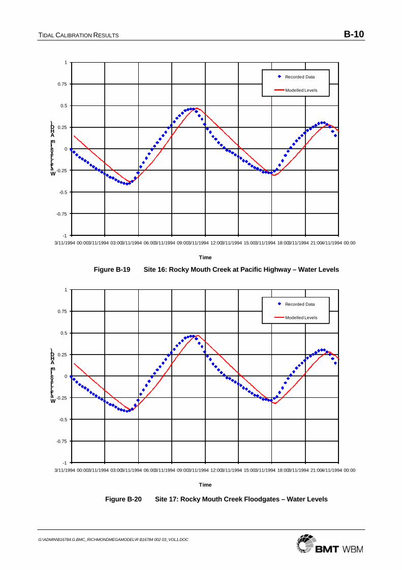
TIDAL CALIBRATION RESULTS B-10
G:\ADMIN\B16784.G.BMC_RICHMONDMEGAMODEL\R B16784 002 03_VOL1.DOC
-1
-0.75
-0.5
-0.25
0
0.25
0.5
0.75
1
3/11/1994 00:003/11/1994 03:003/11/1994 06:003/11/1994 09:003/11/1994 12:003/11/1994 15:003/11/1994 18:003/11/1994 21:004/11/1994 00:00
Water Level (m AHD)
Time
Recorded Data
Modelled Levels
-1
-0.75
-0.5
-0.25
0
0.25
0.5
0.75
1
3/11/1994 00:003/11/1994 03:003/11/1994 06:003/11/1994 09:003/11/1994 12:003/11/1994 15:003/11/1994 18:003/11/1994 21:004/11/1994 00:00
Water Level (m AHD)
Time
Recorded Data
Modelled Levels
Figure B-19 Site 16: Rocky Mouth Creek at Pacific Highway – Water Levels
Figure B-20 Site 17: Rocky Mouth Creek Floodgates – Water Levels
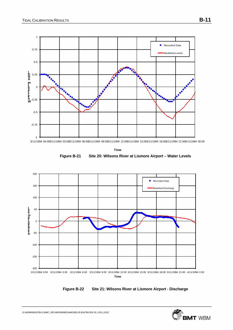
TIDAL CALIBRATION RESULTS B-11
G:\ADMIN\B16784.G.BMC_RICHMONDMEGAMODEL\R B16784 002 03_VOL1.DOC
-1
-0.75
-0.5
-0.25
0
0.25
0.5
0.75
1
3/11/1994 00:003/11/1994 03:003/11/1994 06:003/11/1994 09:003/11/1994 12:003/11/1994 15:003/11/1994 18:003/11/1994 21:004/11/1994 00:00
Water Level (m AHD)
Time
Recorded Data
Modelled Levels
-200
-150
-100
-50
0
50
100
150
200
3/11/1994 0:00 3/11/1994 3:00 3/11/1994 6:00 3/11/1994 9:00 3/11/1994 12:00 3/11/1994 15:00 3/11/1994 18:00 3/11/1994 21:00 4/11/1994 0:00
Discharge (cumecs)
Time
Recorded Data
Modelled Discharge
Figure B-21 Site 20: Wilsons River at Lismore Airport – Water Levels
Figure B-22 Site 21: Wilsons River at Lismore Airport - Discharge
BMT WBM Brisbane Level 11, 490 Upper Edward Street Brisbane 4000
PO Box 203 Spring Hill QLD 4004 Tel +61 7 3831 6744 Fax +61 7 3832 3627 Email [email protected] Web www.wbmpl.com.au
BMT WBM Denver 14 Inverness Drive East, #B132 Englewood Denver Colorado 80112 USA Tel +1 303 792 9814 Fax +1 303 792 9742 Email [email protected] Web www.wbmpl.com.au
BMT WBM Melbourne Level 5, 99 King Street Melbourne 3000 PO Box 604 Collins Street West VIC 8007 Tel +61 3 8620 6100 Fax +61 3 8620 6105 Email [email protected] Web www.wbmpl.com.au
BMT WBM Newcastle 126 Belford Street Broadmeadow 2292 PO Box 266 Broadmeadow NSW 2292 Tel +61 2 4940 8882 Fax +61 2 4940 8887 Email [email protected] Web www.wbmpl.com.au
BMT WBM Perth 1 Brodie Hall Drive Technology Park Bentley 6102 Tel +61 8 9328 2029 Fax +61 8 9486 7588 Email [email protected] Web www.wbmpl.com.au
BMT WBM Sydney Suite 206, 118 Great North Road Five Dock 2046 PO Box 129 Five Dock NSW 2046 Tel +61 2 9713 4836 Fax +61 2 9713 4890 Email [email protected] Web www.wbmpl.com.au
BMT WBM Vancouver 1190 Melville Street #700 Vancouver British Columbia V6E 3W1 Canada Tel +1 604 683 5777 Fax +1 604 608 3232 Email [email protected] Web www.wbmpl.com.au